Principles of Communication Prof. V. Venkata Rao Indian Institute of Technology Madras 7.1 CHAPTER 7 Noise Performance of Various Modulation Schemes 7.1 Introduction The process of (electronic) communication becomes quite challenging because of the unwanted electrical signals in a communications system. These undesirable signals, usually termed as noise, are random in nature and interfere with the message signals. The receiver input, in general, consists of (message) signal plus noise, possibly with comparable power levels. The purpose of the receiver is to produce the desired signal with a signal-to-noise ratio that is above a specified value. In this chapter, we will analyze the noise performance of the modulation schemes discussed in chapters 4 to 6. The results of our analysis will show that, under certain conditions, FM is superior to the linear modulation schemes in combating noise and PCM can provide better signal-to-noise ratio at the receiver output than FM. The trade-offs involved in achieving the superior performance from FM and PCM will be discussed. We shall begin our study with the noise performance of various CW modulations schemes. In this context, it is the performance of the detector (demodulator) that would be emphasized. We shall first develop a suitable receiver model in which the role of the demodulator is the most important one.

Welcome message from author
This document is posted to help you gain knowledge. Please leave a comment to let me know what you think about it! Share it to your friends and learn new things together.
Transcript

Principles of Communication Prof. V. Venkata Rao
Indian Institute of Technology Madras
7.1
CHAPTER 7
Noise Performance of Various Modulation Schemes
7.1 Introduction The process of (electronic) communication becomes quite challenging
because of the unwanted electrical signals in a communications system. These
undesirable signals, usually termed as noise, are random in nature and interfere
with the message signals. The receiver input, in general, consists of (message)
signal plus noise, possibly with comparable power levels. The purpose of the
receiver is to produce the desired signal with a signal-to-noise ratio that is above
a specified value.
In this chapter, we will analyze the noise performance of the modulation
schemes discussed in chapters 4 to 6. The results of our analysis will show that,
under certain conditions, FM is superior to the linear modulation schemes in
combating noise and PCM can provide better signal-to-noise ratio at the receiver
output than FM. The trade-offs involved in achieving the superior performance
from FM and PCM will be discussed.
We shall begin our study with the noise performance of various CW
modulations schemes. In this context, it is the performance of the detector
(demodulator) that would be emphasized. We shall first develop a suitable
receiver model in which the role of the demodulator is the most important one.

Principles of Communication Prof. V. Venkata Rao
Indian Institute of Technology Madras
7.2
7.2 Receiver Model and Figure of Merit: Linear Modulation 7.2.1 Receiver model Consider the superheterodyne receiver shown in Fig. 4.75. To study the
noise performance we shall make use of simplified model shown in Fig. 7.1.
Here, ( )eqH f is the equivalent IF filter which actually represents the cascade
filtering characteristic of the RF, mixer and IF sections of Fig. 4.75. ( )s t is the
desired modulated carrier and ( )w t represents a sample function of the white
Gaussian noise process with the two sided spectral density of N02
. We treat
( )eqH f to be an ideal narrowband, bandpass filter, with a passband between
cf W− to cf W+ for the double sideband modulation schemes. For the case of
SSB, we take the filter passband either between cf W− and cf (LSB) or cf and
cf W+ (USB). (The transmission bandwidth TB is W2 for the double sideband
modulation schemes whereas it is W for the case of SSB). Also, in the present
context, cf represents the carrier frequency measured at the mixer output; that is
c IFf f= .
Fig. 7.1: Receiver model (linear modulation)

Principles of Communication Prof. V. Venkata Rao
Indian Institute of Technology Madras
7.3
The input to the detector is ( ) ( ) ( )x t s t n t= + , where ( )n t is the sample
function of a bandlimited (narrowband) white noise process ( )N t with the power
spectral density ( )NNS f 02
= over the passband of ( )eqH f . (As ( )eqH f is
treated as a narrowband filter, ( )n t represents the sample function of a
narrowband noise process.)
7.2.2 Figure-of-merit The performance of analog communication systems are measured in
terms of Signal-to-Noise Ratio ( )SNR . The SNR measure is meaningful and
unambiguous provided the signal and noise are additive at the point of
measurement. We shall define two ( )SNR quantities, namely, (i) ( )SNR 0 and
(ii) ( )rSNR .
The output signal-to-noise ratio is defined as,
( )SNR 0Average power of the message at receiver output
Average noise power at the receiver output= (7.1)
The reference signal-to-noise ratio is defined as,
( )rSNR
Average power of the modulatedmessage signal at receiver input
Average noise power in the messagebandwidth at receiver input
⎛ ⎞⎜ ⎟⎝ ⎠=
⎛ ⎞⎜ ⎟⎝ ⎠
(7.2)
The quantity, ( )rSNR can be viewed as the output signal-to-noise ratio which
results from baseband or direct transmission of the message without any
modulation as shown in Fig. 7.2. Here, ( )m t is the baseband message signal
with the same power as the modulated wave. For the purpose of comparing
different modulation systems, we use the Figure-of-Merit ( )FOM defined as,

Principles of Communication Prof. V. Venkata Rao
Indian Institute of Technology Madras
7.4
( )( )rSNR
FOMSNR
0= (7.3)
Fig. 7.2: Ideal Baseband Receiver
FOM as defined above provides a normalized ( )SNR 0 performance of
the various modulation-demodulation schemes; larger the value of FOM, better is
the noise performance of the given communication system.
Before analyzing the SNR performance of various detectors, let us
quantify the outputs expected of the (idealized) detectors when the input is a
narrowband signal. Let ( )x t be a real narrowband bandpass signal. From Eq.
1.55, ( )x t can be expressed as
( )( ) ( ) ( ) ( ) ( )
( ) ( ) ( )
c c s c
c
x t t x t tx t
A t t t
cos sin 7.4a
cos 7.4b
⎧ ω − ω⎪= ⎨⎡ ⎤ω + ϕ⎪ ⎣ ⎦⎩
( )cx t and ( )sx t are the in-phase and quadrature components of ( )x t . The
envelope ( )A t and the phase ( )tϕ are given by Eq. 1.56. In this chapter, we will
analyze the performance of a coherent detector, envelope detector, phase
detector and a frequency detector when signals such as ( )x t are given as input.
The outputs of the (idealized) detectors can be expressed mathematically in
terms of the quantities involved in Eq. 7.4. These are listed below. (Table 7.1)
Principles of Communication Prof. V. Venkata Rao
Indian Institute of Technology Madras
7.5
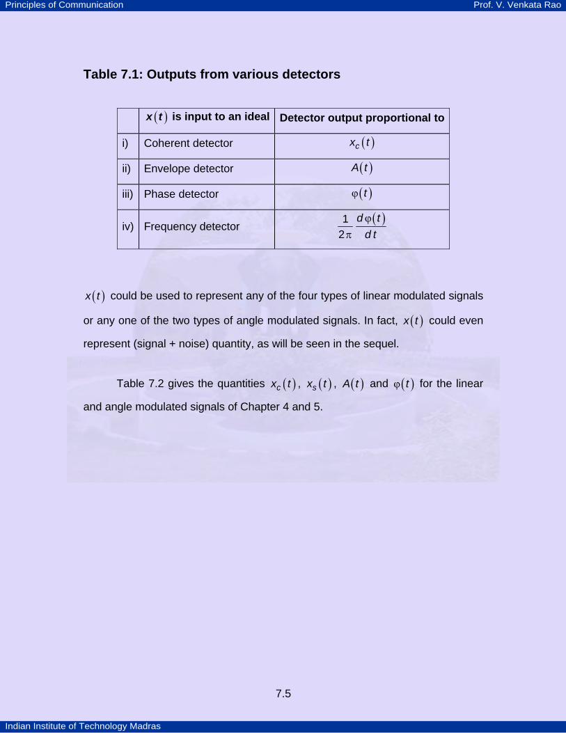
Table 7.1: Outputs from various detectors
( )x t is input to an ideal Detector output proportional to
i) Coherent detector ( )cx t
ii) Envelope detector ( )A t
iii) Phase detector ( )tϕ
iv) Frequency detector ( )d t
d t1
2ϕ
π
( )x t could be used to represent any of the four types of linear modulated signals
or any one of the two types of angle modulated signals. In fact, ( )x t could even
represent (signal + noise) quantity, as will be seen in the sequel.
Table 7.2 gives the quantities ( )cx t , ( )sx t , ( )A t and ( )tϕ for the linear
and angle modulated signals of Chapter 4 and 5.

Principles of Communication Prof. V. Venkata Rao
Indian Institute of Technology Madras
7.6
Table 7.2: Components of linear and angle modulated signals Signal ( )cx t ( )sx t ( )A t ( )tϕ
1 DSB-SC
( ) ( )c cA m t tcos ω ( )cA m t zero ( )cA m t
( )m t0, 0>
( )m t, 0π <
2 DSB-LC (AM)
( )[ ] ( )c m cA g m t t1 cos+ ω ,
( )[ ]c mA g m t1 0+ ≥
( )[ ]c mA g m t1 + zero ( )[ ]c mA g m t1 + zero
3 SSB
( ) ( )
( ) ( )
cc
cc
A m t t
A m t t
cos2
sin2
ω
± ω
( )cA m t
2 ( )cA m t
2± ( ) ( )cA
m t tm2 2
2+
( )( )
m t
m t1tan− −⎡ ⎤⎢ ⎥⎣ ⎦
4 Phase modulation
( )[ ]c cA t tcos ω + ϕ ,
( ) ( )pt k m tϕ =
( )cA tcosϕ ( )cA tsinϕ cA ( )pk m t
5 Frequency modulation
( )[ ]c cA t tcos ω + ϕ ,
( ) ( )t
ft k m d2− ∞
ϕ = π τ τ∫
( )cA tcosϕ ( )cA tsinϕ cA ( )t
fk m d2− ∞
π τ τ∫
Example 7.1
Let ( ) ( ) ( )c m cs t A t tcos cos= ω ω where mf310= Hz and cf
610= Hz.
Let us compute and sketch the output ( )v t of an ideal frequency detector when
( )s t is its input.
From Table 7.1, we find that an ideal frequency detector output will be
proportional to ( )d td t
12
ϕπ
. For the DSB-SC signal,

Principles of Communication Prof. V. Venkata Rao
Indian Institute of Technology Madras
7.7
( )( )( )
m tt
m t
0 , 0
, 0
⎧ >⎪ϕ = ⎨π <⎪⎩
For the example, ( ) ( )m t t3cos 2 10⎡ ⎤= π ×⎣ ⎦. Hence ( )tϕ is shown in Fig. 7.3(b).
Fig. 7.3: (Ideal) frequency detector output of example 7.1
Differentiating the waveform in (b), we obtain ( )v t , which consists of a
sequence of impulses which alternate in polarity, as shown in (c).

Principles of Communication Prof. V. Venkata Rao
Indian Institute of Technology Madras
7.8
Example 7.2
Let ( )m tt2
11
=+
. Let ( )s t be an SSB signal with ( )m t as the message
signal. Assuming that ( )s t is the input to an ideal ED, let us find the expression
for its output ( )v t .
From Example 1.24, we have
( )m tt2
11
=+
As the envelope of ( )s t is ( ) ( )m t m t
122 2⎧ ⎫⎡ ⎤⎡ ⎤ +⎨ ⎬⎣ ⎦ ⎣ ⎦⎩ ⎭
, we have
( )v tt2
1
1=
+.
7.3 Coherent Demodulation 7.3.1 DSB-SC The receiver model for coherent detection of DSB-SC signals is shown in
Fig. 7.4. The DSB-SC signal is, ( ) ( ) ( )c cs t A m t tcos= ω . We assume ( )m t to
be sample function of a WSS process ( )M t with the power spectral density,
( )MS f , limited to W± Hz.
Fig. 7.4: Coherent Detection of DSB-SC.

Principles of Communication Prof. V. Venkata Rao
Indian Institute of Technology Madras
7.9
The carrier, ( )c cA tcos ω , which is independent of the message ( )m t is actually
a sample function of the process ( )c cA tcos ω + Θ where Θ is a random
variable, uniformly distributed in the interval 0 to 2 π . With the random phase
added to the carrier term, ( )sR τ , the autocorrelation function of the process ( )S t
(of which ( )s t is a sample function), is given by,
( ) ( ) ( )cs M c
AR R2
cos2
τ = τ ω τ (7.5a)
where ( )MR τ is the autocorrelation function of the message process. Fourier
transform of ( )sR τ yields ( )sS f given by,
( ) ( ) ( )cs M c M c
AS f S f f S f f2
4⎡ ⎤= − + +⎣ ⎦ (7.5b)
Let MP denote the message power, where
( ) ( )W
M M MW
P S f d f S f d f∞
− ∞ −
= =∫ ∫
Then, ( ) ( )c
c
f Wc c M
s M cf W
A A PS f d f S f f d f2 2
24 2
+∞
− ∞ −
= − =∫ ∫ .
That is, the average power of the modulated signal ( )s t is c MA P2
2. With the (two
sided) noise power spectral density of N02
, the average noise power in the
message bandwidth W2 is NW W N002
2× = . Hence,
( ) c Mr DSB SC
A PSNRW N
2
02−⎡ ⎤ =⎣ ⎦ (7.6)
To arrive at the FOM , we require ( )SNR 0 . The input to the detector is
( ) ( ) ( )x t s t n t= + , where ( )n t is a narrowband noise quantity. Expressing ( )n t
in terms of its in-phase and quadrature components, we have

Principles of Communication Prof. V. Venkata Rao
Indian Institute of Technology Madras
7.10
( ) ( ) ( ) ( ) ( ) ( )c c c c s cx t A m t t n t t n tcos cos sin= ω + ω − ω
Assuming that the local oscillator output is ( )c tcos ω , the output ( )v t of the
multiplier in the detector (Fig. 7.4) is given by
( ) ( ) ( ) ( ) ( ) ( )
( ) ( )
c c c c c
c s c
v t A m t n t A m t n t t
A n t t
1 1 1 cos 22 2 2
1 sin 22
⎡ ⎤= + + + ω⎣ ⎦
− ω
As the LPF rejects the spectral components centered around cf2 , we have
( ) ( ) ( )c cy t A m t n t1 12 2
= + (7.7)
From Eq. 7.7, we observe that,
i) Signal and noise which are additive at the input to the detector are additive
even at the output of the detector
ii) Coherent detector completely rejects the quadrature component ( )sn t .
iii) If the noise spectral density is flat at the detector input over the passband
( )c cf W f W,− + , then it is flat over the baseband ( )W W,− , at the
detector output. (Note that ( )cn t has a flat spectrum in the range W− to
W .)
As the message component at the output is ( )cA m t12
⎛ ⎞⎜ ⎟⎝ ⎠
, the average
message power at the output is cM
A P2
4⎛ ⎞⎜ ⎟⎜ ⎟⎝ ⎠
. As the spectral density of the in-phase
noise component is N0 for f W≤ , the average noise power at the receiver
output is ( ) W NW N 00
1 24 2
⋅ = . Therefore,
( )( )( )
c M
DSB SC
A PSNR
W N
2
00
4
2−⎡ ⎤ =⎣ ⎦

Principles of Communication Prof. V. Venkata Rao
Indian Institute of Technology Madras
7.11
c MA PW N
2
02= (7.8)
From Eq. 7.6 and 7.8, we obtain
[ ] ( )( )DSB SC
r
SNRFOM
SNR0 1− = = (7.9)
7.3.2 SSB Assuming that LSB has been transmitted, we can write ( )s t as follows:
( ) ( ) ( ) ( ) ( )c cc c
A As t m t t m t tcos sin2 2
= ω + ω
where ( )m t is the Hilbert transform of ( )m t . Generalizing,
( ) ( ) ( ) ( ) ( )c cc c
A AS t M t t M t tcos sin2 2
= ω + ω .
We can show that the autocorrelation function of ( )S t , ( )sR τ is given by
( ) ( ) ( ) ( ) ( )c Ms M c cAR R R
2cos sin
4⎡ ⎤τ = τ ω τ + τ ω τ⎣ ⎦
where ( )MR t is the Hilbert transform of ( )MR t . Hence the average signal
power, ( ) cs M
AR P2
04
=
and ( ) c Mr
A PSNRW N
2
04= (7.10)
Let ( ) ( ) ( ) ( ) ( )c c s cn t n t t n t tcos sin= ω − ω
(Note that with respect to cf , ( )n t does not have a locally symmetric spectrum).
( ) ( ) ( )c cy t A m t n t1 14 2
= +
Hence, the output signal power is c MA P2
16 and the output noise power as
W N014
⎛ ⎞⎜ ⎟⎝ ⎠
. Thus, we obtain,

Principles of Communication Prof. V. Venkata Rao
Indian Institute of Technology Madras
7.12
( ) c MSSB
A PSNRW N
2
0,0
416
= ×
c MA PW N
2
04= (7.11)
From Eq. 7.10 and 7.11,
( )SSBFOM 1= (7.12)
From Eq. 7.9 and 7.12, we find that under synchronous detection, SNR
performance of DSB-SC and SSB are identical, when both the systems operate
with the same signal-to-noise ratio at the input of their detectors.
In arriving at the RHS of Eq. 7.11, we have used the narrowband noise
description with respect to cf . We can arrive at the same result, if the noise
quantity is written with respect to the centre frequency cWf2
⎛ ⎞−⎜ ⎟⎝ ⎠
.
7.4 Envelope Detection DSB-LC or AM signals are normally envelope detected, though coherent
detection can also be used for message recovery. This is mainly because
envelope detection is simpler to implement as compared to coherent detection.
We shall now compute the ( )AMFOM .
The transmitted signal ( )s t is given by
( ) ( ) ( )c m cs t A g m t t1 cos⎡ ⎤= + ω⎣ ⎦
Then the average signal power in ( ) c m MA g Ps t
2 21
2
⎡ ⎤+⎣ ⎦= . Hence
( )( )c m M
r DSB LC
A g PSNR
W N
2 2
,0
1
2−
+= (7.13)
Principles of Communication Prof. V. Venkata Rao
Indian Institute of Technology Madras
7.13
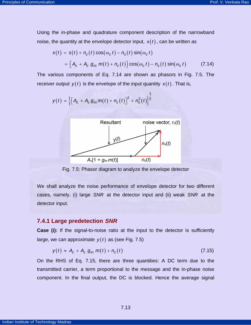
Using the in-phase and quadrature component description of the narrowband
noise, the quantity at the envelope detector input, ( )x t , can be written as
( ) ( ) ( ) ( ) ( ) ( )c c s cx t s t n t t n t tcos sin= + ω − ω
( ) ( ) ( ) ( ) ( )c c m c c s cA A g m t n t t n t tcos sin⎡ ⎤= + + ω − ω⎣ ⎦ (7.14)
The various components of Eq. 7.14 are shown as phasors in Fig. 7.5. The
receiver output ( )y t is the envelope of the input quantity ( )x t . That is,
( ) ( ) ( ) ( ){ }c c m c sy t A A g m t n t n t1
2 22⎡ ⎤= + + +⎣ ⎦
Fig. 7.5: Phasor diagram to analyze the envelope detector
We shall analyze the noise performance of envelope detector for two different
cases, namely, (i) large SNR at the detector input and (ii) weak SNR at the
detector input.
7.4.1 Large predetection SNR Case (i): If the signal-to-noise ratio at the input to the detector is sufficiently
large, we can approximate ( )y t as (see Fig. 7.5)
( ) ( ) ( )c c m cy t A A g m t n t≈ + + (7.15)
On the RHS of Eq. 7.15, there are three quantities: A DC term due to the
transmitted carrier, a term proportional to the message and the in-phase noise
component. In the final output, the DC is blocked. Hence the average signal
Principles of Communication Prof. V. Venkata Rao
Indian Institute of Technology Madras
7.14
power at the output is given by c m MA g P2 2 . The output noise power being equal
to W N02 we have,
( ) c m MAM
A g PSNRW N
2 2
002
⎡ ⎤ ≈⎣ ⎦ (7.16)
It is to be noted that the signal and noise are additive at the detector output and
power spectral density of the output noise is flat over the message bandwidth.
From Eq. 7.13 and 7.16 we obtain,
( ) m MAM
m m
g PFOMg P
2
21=
+ (7.17)
As can be seen from Eq. 7.17, the FOM with envelope detection is less than
unity. That is, the noise performance of DSB-LC with envelope detection is
inferior to that of DSB-SC with coherent detection. Assuming ( )m t to be a tone
signal, ( )m mA tcos ω and m mg Aµ = , simple calculation shows that ( )AMFOM is
( )2
22µ
+ µ. With the maximum permitted value of 1µ = , we find that the
( )AMFOM is 13
. That is, other factors being equal, DSB-LC has to transmit three
times as much power as DSB-SC, to achieve the same quality of noise
performance. Of course, this is the price one has to pay for trying to achieve
simplicity in demodulation.
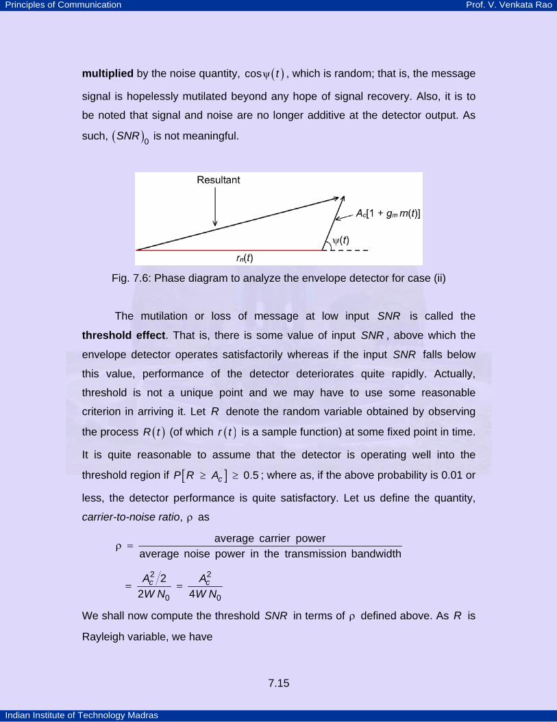
7.4.2 Weak predetection SNR
In this case, noise term dominates. Let ( ) ( ) ( )n cn t r t t tcos ⎡ ⎤= ω + ψ⎣ ⎦ . We
now construct the phasor diagram using ( )nr t as the reference phasor (Fig. 7.6).
Envelope detector output can be approximated as
( ) ( ) ( ) ( ) ( )n c c my t r t A t A g m t tcos cos⎡ ⎤ ⎡ ⎤≈ + ψ + ψ⎣ ⎦ ⎣ ⎦ (7.18)
From Eq. 7.18, we find that detector output has no term strictly proportional to
( )m t . The last term on the RHS of Eq. 7.18 contains the message signal ( )m t
Principles of Communication Prof. V. Venkata Rao
Indian Institute of Technology Madras
7.15
multiplied by the noise quantity, ( )tcosψ , which is random; that is, the message
signal is hopelessly mutilated beyond any hope of signal recovery. Also, it is to
be noted that signal and noise are no longer additive at the detector output. As
such, ( )SNR 0 is not meaningful.
Fig. 7.6: Phase diagram to analyze the envelope detector for case (ii)
The mutilation or loss of message at low input SNR is called the
threshold effect. That is, there is some value of input SNR , above which the
envelope detector operates satisfactorily whereas if the input SNR falls below
this value, performance of the detector deteriorates quite rapidly. Actually,
threshold is not a unique point and we may have to use some reasonable
criterion in arriving it. Let R denote the random variable obtained by observing
the process ( )R t (of which ( )r t is a sample function) at some fixed point in time.
It is quite reasonable to assume that the detector is operating well into the
threshold region if [ ]cP R A 0.5≥ ≥ ; where as, if the above probability is 0.01 or
less, the detector performance is quite satisfactory. Let us define the quantity,
carrier-to-noise ratio, ρ as
average carrier poweraverage noise power in the transmission bandwidth
ρ =
c cA AW N W N
2 2
0 0
22 4
= =
We shall now compute the threshold SNR in terms of ρ defined above. As R is
Rayleigh variable, we have
Principles of Communication Prof. V. Venkata Rao
Indian Institute of Technology Madras
7.16
( ) N
r
RN
rf r e
2
222
−σ=
σ
where N W N202σ =
[ ] ( )c
c RA
P R A f r d r∞
≥ = ∫
cA
W Ne
2
04−
=
e− ρ=
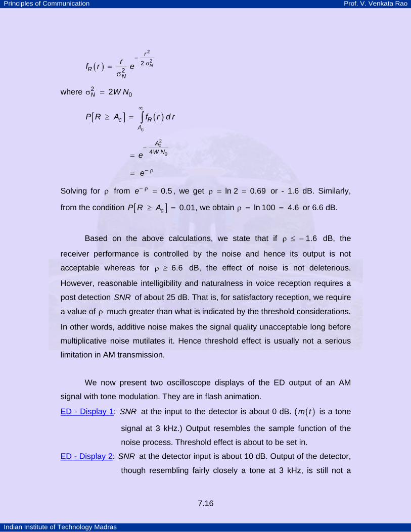
Solving for ρ from e 0.5− ρ = , we get ln 2 0.69ρ = = or - 1.6 dB. Similarly,
from the condition [ ]cP R A 0.01≥ = , we obtain ln 100 4.6ρ = = or 6.6 dB.
Based on the above calculations, we state that if 1.6ρ ≤ − dB, the
receiver performance is controlled by the noise and hence its output is not
acceptable whereas for 6.6ρ ≥ dB, the effect of noise is not deleterious.
However, reasonable intelligibility and naturalness in voice reception requires a
post detection SNR of about 25 dB. That is, for satisfactory reception, we require
a value of ρ much greater than what is indicated by the threshold considerations.
In other words, additive noise makes the signal quality unacceptable long before
multiplicative noise mutilates it. Hence threshold effect is usually not a serious
limitation in AM transmission.
We now present two oscilloscope displays of the ED output of an AM
signal with tone modulation. They are in flash animation.
TUED - Display 1UT: SNR at the input to the detector is about 0 dB. ( ( )m t is a tone
signal at 3 kHz.) Output resembles the sample function of the
noise process. Threshold effect is about to be set in.
TUED - Display 2UT: SNR at the detector input is about 10 dB. Output of the detector,
though resembling fairly closely a tone at 3 kHz, is still not a

Principles of Communication Prof. V. Venkata Rao
Indian Institute of Technology Madras
7.17
pure tone signal. Some amount of noise is seen riding on the
output sine wave and the peaks of the sinewave are not
perfectly aligned.
Example 7.3
In a receiver meant for the demodulation of SSB signals, ( )eqH f has the
characteristic shown in Fig. 7.7. Assuming that USB has been transmitted, let us
find the FOM of the system.
Fig. 7.7: ( )eqH f for the Example 7.3
Because of the non-ideal ( )eqH f , ( )cNS f will be as shown in Fig. 7.8.
Fig. 7.8: ( )cNS f of Example 7.3
For SSB with coherent demodulation, we have

Principles of Communication Prof. V. Venkata Rao
Indian Institute of Technology Madras
7.18
Signal quantity at the output ( )cA m t4
=
Noise quantity at the output ( )cn t2
=
Output noise power c
W
NW
S d f14
−
= ∫
N W05
16=
( )c MA P
SNRN W
2
00
165
16
⎛ ⎞⎜ ⎟⎜ ⎟⎝ ⎠=
c MA PN W
2
05=
( ) c Mr
A PSNRW N
2
04=
Hence ( )( )rSNR
FOMSNR
0 4 0.85
= = = .
Principles of Communication Prof. V. Venkata Rao
Indian Institute of Technology Madras
7.19
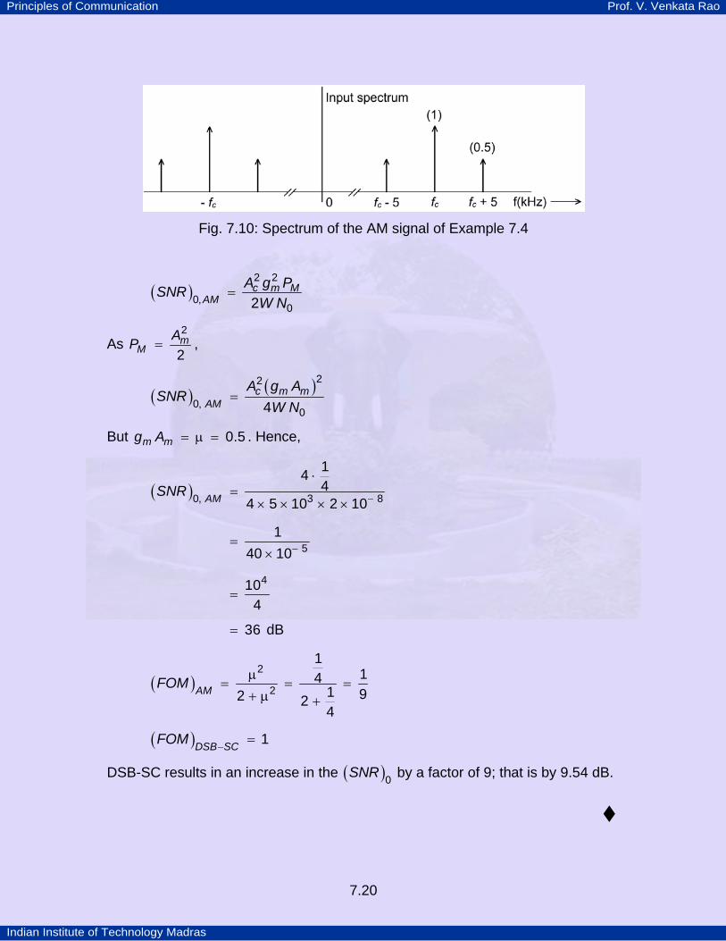
Example 7.4 In a laboratory experiment involving envelope detection, AM signal at the
input to ED, has the modulation index 0.5 with the carrier amplitude of 2 V. ( )m t
is a tone signal of frequency 5 kHz and cf 5>> kHz. If the (two-sided) noise
PSD at the detector input is 810− Watts/Hz, what is the expected ( )SNR 0 of this
scheme? By how many dB, this scheme is inferior to DSB-SC?
Spectrum of the AM signal is as shown in Fig. 7.10.
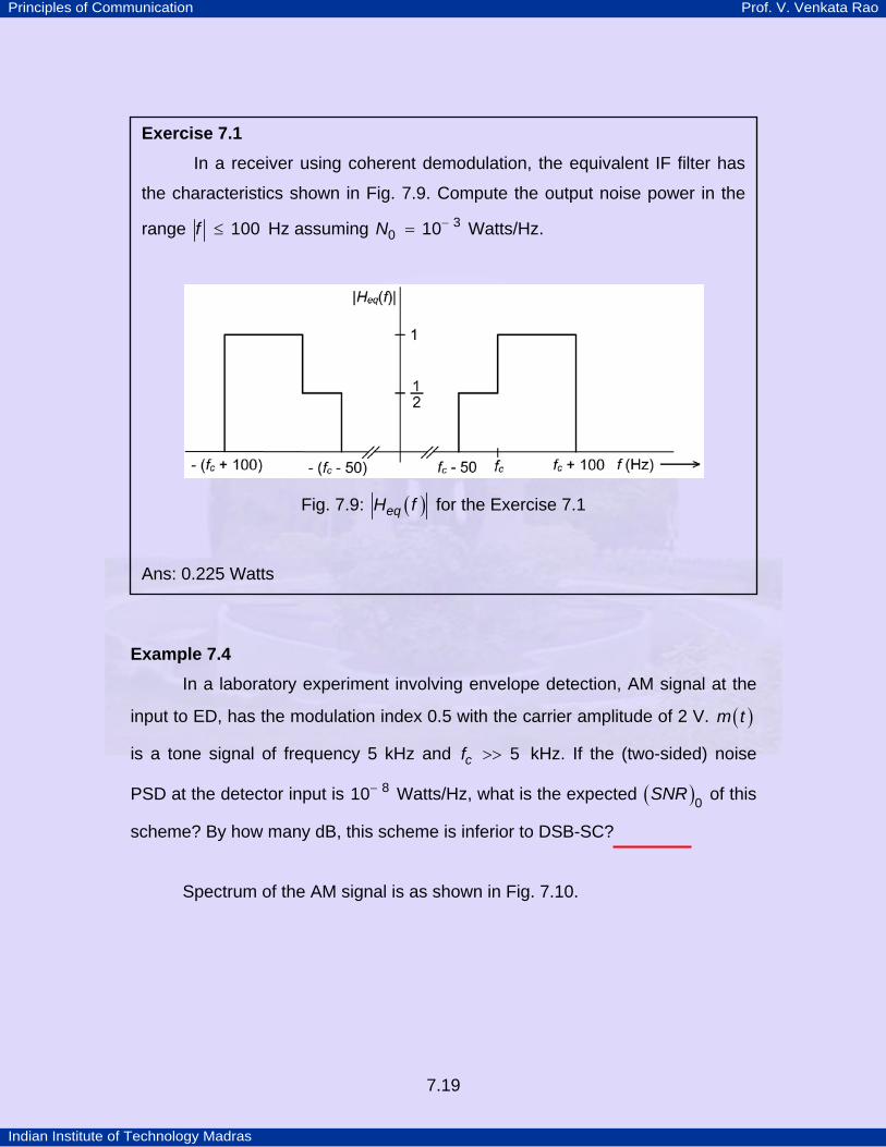
Exercise 7.1 In a receiver using coherent demodulation, the equivalent IF filter has
the characteristics shown in Fig. 7.9. Compute the output noise power in the
range f 100≤ Hz assuming N 30 10−= Watts/Hz.
Fig. 7.9: ( )eqH f for the Exercise 7.1
Ans: 0.225 Watts
Principles of Communication Prof. V. Venkata Rao
Indian Institute of Technology Madras
7.20
Fig. 7.10: Spectrum of the AM signal of Example 7.4
( ) c m MAM
A g PSNRW N
2 2
0,02
=
As mM
AP2
2= ,
( ) ( )c m mAM
A g ASNR
W N
22
0,04
=
But m mg A 0.5= µ = . Hence,
( ) AMSNR 3 80,
144
4 5 10 2 10−
⋅=
× × × ×
51
40 10−=
×
410
4=
36= dB
( )AMFOM2
2
114
1 92 24
µ= = =
+ µ +
( )DSB SCFOM 1− =
DSB-SC results in an increase in the ( )SNR 0 by a factor of 9; that is by 9.54 dB.
Principles of Communication Prof. V. Venkata Rao
Indian Institute of Technology Madras
7.21
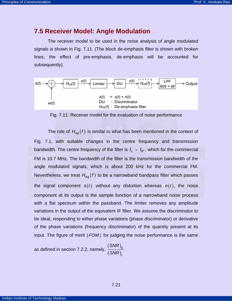
7.5 Receiver Model: Angle Modulation The receiver model to be used in the noise analysis of angle modulated
signals is shown in Fig. 7.11. (The block de-emphasis filter is shown with broken
lines; the effect of pre-emphasis, de-emphasis will be accounted for
subsequently).
Fig. 7.11: Receiver model for the evaluation of noise performance
The role of ( )eqH f is similar to what has been mentioned in the context of
Fig. 7.1, with suitable changes in the centre frequency and transmission
bandwidth. The centre frequency of the filter is c IFf f= , which for the commercial
FM is 10.7 MHz. The bandwidth of the filter is the transmission bandwidth of the
angle modulated signals, which is about 200 kHz for the commercial FM.
Nevertheless, we treat ( )eqH f to be a narrowband bandpass filter which passes
the signal component ( )s t without any distortion whereas ( )n t , the noise
component at its output is the sample function of a narrowband noise process
with a flat spectrum within the passband. The limiter removes any amplitude
variations in the output of the equivalent IF filter. We assume the discriminator to
be ideal, responding to either phase variations (phase discriminator) or derivative
of the phase variations (frequency discriminator) of the quantity present at its
input. The figure of merit ( )FOM for judging the noise performance is the same
as defined in section 7.2.2, namely, ( )( )rSNRSNR
0 .

Principles of Communication Prof. V. Venkata Rao
Indian Institute of Technology Madras
7.22
7.6 Calculation of FOM Let,
( ) ( )c cs t A t tcos ⎡ ⎤= ω + ϕ⎣ ⎦ (7.19)
where
( )( ) ( )
( ) ( )
pt
f
k m t
tk m d
, forPM 7.20a
2 , for FM 7.20b− ∞
⎧ ⋅ ⋅ ⋅⎪⎪ϕ = ⎨
π τ τ ⋅ ⋅ ⋅⎪⎪⎩
∫
The output of ( )eqH f is,
( ) ( ) ( )x t s t n t= + (7.21a)
( ) ( ) ( )c c n cA t t r t t tcos cos⎡ ⎤ ⎡ ⎤= ω + ϕ + ω + ψ⎣ ⎦ ⎣ ⎦ (7.21b)
where, on the RHS of Eq. 7.21(b) we have used the envelope ( )( )nr t and phase
( )( )tψ representation of the narrowband noise. As in the case of envelope
detection of AM, we shall consider two cases:
i) Strong predetection SNR , ( )( )>>c nA r t most of the time and
ii) Weak predetection SNR , ( )( )<<c nA r t most of the time .
7.6.1 Strong Predetection SNR Consider the phasor diagram shown in Fig. 7.12, where we have used the
unmodulated carrier as the reference. ( )r t represents the envelope of the
resultant (signal + noise) phasor and ( )tθ , the phase angle of the resultant. As
far as this analysis is concerned, ( )r t is of no consequence (any variations in
( )r t are taken care of by the limiter). We express ( )tθ as
( ) ( ) ( ) ( ) ( )( ) ( ) ( )
n
c n
r t t tt t
A r t t t1 sin
tancos
− ⎧ ⎫⎡ ⎤ψ − ϕ⎪ ⎪⎣ ⎦θ = ϕ + ⎨ ⎬⎡ ⎤+ ψ − ϕ⎪ ⎪⎣ ⎦⎩ ⎭ (7.22a)

Principles of Communication Prof. V. Venkata Rao
Indian Institute of Technology Madras
7.23
Fig. 7.12: Phasor diagram for the case of strong predetection SNR.
If we make the assumption that ( )c nA r t>> most of the time, we can write,
( ) ( ) ( ) ( ) ( )n
c
r tt t t t
Asin ⎡ ⎤θ ≈ ϕ + ψ − ϕ⎣ ⎦ (7.22b)
Notice that the second term on the RHS of Eq. 7.22(b) has the factor ( )n
c
r tA
. Thus
when the FM signal is much stronger than the noise, it will suppress the small
random phase variations caused by noise; then the FM signal is said to capture
the detector. ( )v t , the output of the discriminator is given by,
( ) ( )dv t k t= θ (phase detector)
( )d d tkd t2θ
=π
(frequency detector)
where dk is the gain constant of the detector under consideration.
a) Phase Modulation
For PM, ( ) ( )pt k m tϕ = . For convenience, let p dk k 1= . Then,
( ) ( ) ( ) ( ) ( )d n
c
k r tv t m t t t
Asin ⎡ ⎤≈ + ψ − ϕ⎣ ⎦ (7.23)
Again, we treat ( )m t to be a sample function of a WSS process ( )M t . Then,

Principles of Communication Prof. V. Venkata Rao
Indian Institute of Technology Madras
7.24
output signal power = ( ) ( )M MP M t R2 0= = (7.24)
Let ( ) ( ) ( ) ( )d nP
c
k r tn t t t
Asin ⎡ ⎤= ψ − ϕ⎣ ⎦ (7.25)
To calculate the output noise power, we require the power spectral density
of ( )Pn t . This is made somewhat difficult because of ( )tϕ in ( )Pn t . The analysis
becomes fairly easy if we assume ( )t 0ϕ = . Of course, it is possible to derive
the PSD of ( )Pn t without making the assumption that ( )t 0ϕ = . This has been
done in Appendix A7.1. In this appendix, it has been shown that the effect of
( )tϕ is to produce spectral components beyond W , which are anyway removed
by the final, LPF. Hence, we proceed with our analysis by setting ( )t 0ϕ = on
the RHS of Eq. 7.25. Then ( )Pn t reduces to,
( ) ( ) ( )d nP
c
k r tn t t
Asin ⎡ ⎤= ψ⎣ ⎦
( )ds
c
k n tA
=
Hence,
( ) ( )P s
dN N
c
kS f S fA
2⎛ ⎞
= ⎜ ⎟⎝ ⎠
But, ( )s
T
N
BN fS f
otherwise
0 ,2
0 ,
⎧ ≤⎪= ⎨⎪⎩
TB is the transmission bandwidth, which for the PM case can be taken as the
value given by Eq. 5.26.
Post detection LPF passes only those spectral components that are within
( )W W,− . Hence the output noise power d
c
k W NA
2
02⎛ ⎞
= ⎜ ⎟⎝ ⎠
, resulting in,
Principles of Communication Prof. V. Venkata Rao
Indian Institute of Technology Madras
7.25
( ) MPM
d
c
PSNRkW NA
20,
02
=⎛ ⎞⎜ ⎟⎝ ⎠
cp M
A k PW N
22
02= (7.26)
As, ( )( )c
r PM
ASNR
N W
2
,0
2=
we have,
( ) ( )( ) p MPM
r
SNRFOM k P
SNR20= = (7.27a)
We can express ( )PMFOM in terms of the RMS bandwidth. From Eq. A5.4.7,
(Appendix A5.4), we have
( ) ( ) ( )rms p M rmsPM MB k R B2 0=
( )p M rms Mk P B2=
Hence ( )( )
rms PMp M
rms M
Bk P
B
2
22
4=
Using this value in Eq. 7.27(a), we obtain
( )( )( )
rms PMPM
rms M
BFOM
B
2
24
⎡ ⎤⎣ ⎦=⎡ ⎤⎣ ⎦
(7.27b)
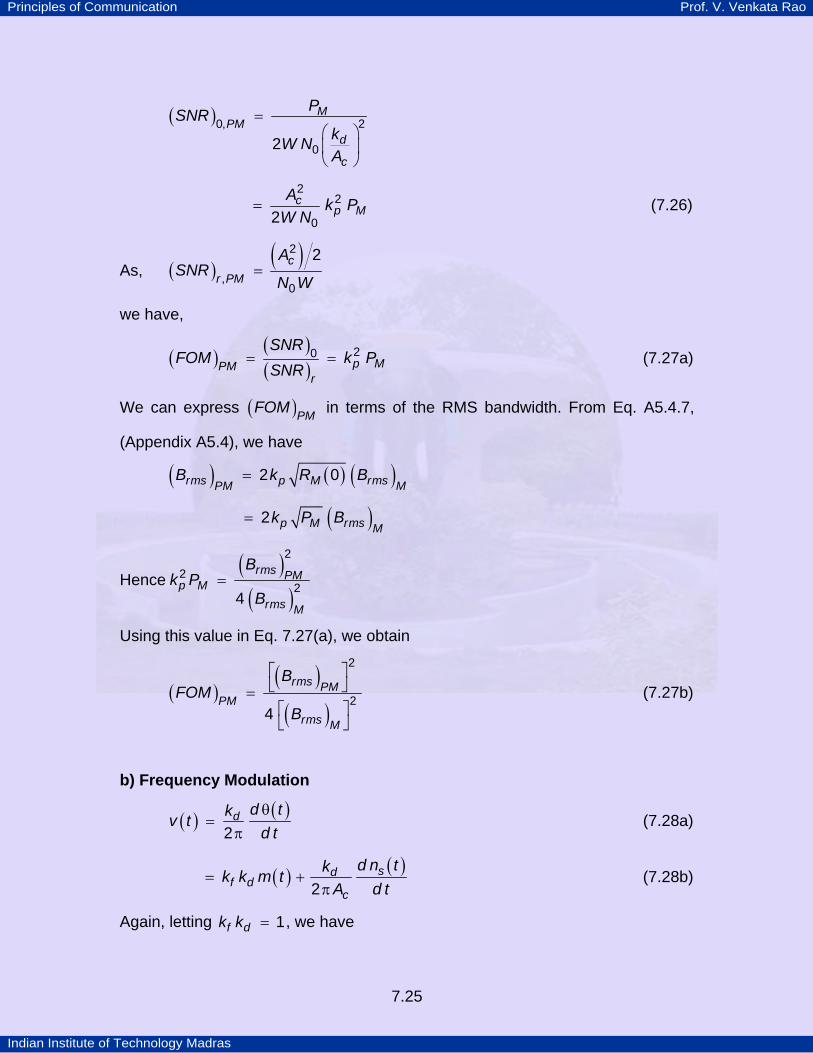
b) Frequency Modulation
( ) ( )d d tkv td t2θ
=π
(7.28a)
( ) ( )sdf d
c
d n tkk k m tA d t2
= +π
(7.28b)
Again, letting f dk k 1= , we have
Principles of Communication Prof. V. Venkata Rao
Indian Institute of Technology Madras
7.26
( ) ( ) ( )sd
c
d n tkv t m tA d t2
= +π
output signal power MP=
Let ( ) ( )sdF
c
d n tkn tA d t2
=π
Then, ( ) ( )F S
dN N
c
kS f j f S fA
222
2⎛ ⎞
= π⎜ ⎟π⎝ ⎠
The above step follows from the fact that ( )sd n td t
can be obtained by
passing ( )sn t through a differentiator with the transfer function j f2π . Thus,
( ) ( )F S
dN N
c
k fS f S fA
2 2
2=
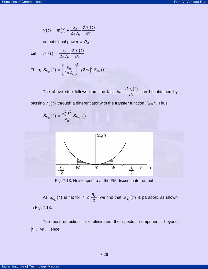
Fig. 7.13: Noise spectra at the FM discriminator output
As ( )SNS f is flat for TBf
2≤ , we find that ( )
FNS f is parabolic as shown
in Fig. 7.13.
The post detection filter eliminates the spectral components beyond
f W> . Hence,

Principles of Communication Prof. V. Venkata Rao
Indian Institute of Technology Madras
7.27
The output noise power W
d
cW
k f N d fA
2 20
2−
= ∫
d
c
k N WA
230
223
⎛ ⎞= ⎜ ⎟⎝ ⎠
(7.29)
This is equal to the hatched area in Fig 7.13.
Again, as in the case of PM, we find that increasing the carrier power has
a noise quietening effect. But, of course, there is one major difference between
( )PNS f and ( )
FNS f ; namely, the latter is parabolic whereas the former is a fiat
spectrum.
The parabolic nature of the output FM noise spectrum implies, that high
frequency end of the message spectrum is subject to stronger degradation
because of noise. Completing our analysis, we find that
( ) c MFM
d
A PSNRk N W
2
2 30,0
32
= (7.30a)
c Mf
A PkN W
22
30
32
= (7.30b)
c f MA k PN W W
2 2
20
32
⎛ ⎞= ⎜ ⎟⎜ ⎟⎝ ⎠
(7.30c)
Let us express ( )FMFOM in terms of ( )rms FMB . From Appendix A5.4, Eq. A5.4.5,
( ) ( )rms f MFMB k R2 0=
f Mk P2=
That is, ( )rms FM
f M
Bk P
2
24
⎡ ⎤⎣ ⎦=

Principles of Communication Prof. V. Venkata Rao
Indian Institute of Technology Madras
7.28
Hence, ( )( )rmsc FM
FM
BASNRN W W
22
0,0
32 4
⎡ ⎤⎢ ⎥=⎢ ⎥⎣ ⎦
As ( )rSNR is the same as in the case of PM, we have
( )( )rmsf M FM
FM
Bk PFOMWW
22
2334
⎡ ⎤⎢ ⎥= =⎢ ⎥⎣ ⎦
(7.31)
For a given peak value of the input signal, we find that the deviation ratio D is
proportional to fkW
; hence ( )FMFOM is a quadratic function of D . The price paid
to achieve a significant value for the FOM is the need for increased transmission
bandwidth, ( )TB D k W2= + . Of course, we should not forget the fact that the
result of Eq. 7.31 is based on the assumption that SNR at the detector input is
sufficiently large.
How do we justify that increasing D , (that is, the transmission bandwidth),
will result in the improvement of the output SNR ? Let us look at Eq. 7.28(b). On
the RHS, we have two quantities, namely ( )f dk k m t and ( )sd
c
d n tkA d t2π
. The
latter quantity is dependent only on noise and is independent of the message
signal. d
c
kA2π
being a constant, ( )sd n td t
is the quantity that causes the
perturbation of the instantaneous frequency due to the noise. Let us that assume
that it is less than or equal to ( )nf∆ , most of the time. For a given detector, dk is
fixed. Hence, as fk increases, frequency deviation increases, thereby increasing
the value of D . Let f fk k,2 ,1> . Then, to transmit the same ( )m t , we require
more bandwidth if we use a modulator with the frequency sensitivity fk ,2 instead
of fk ,1. In other words, ( ) ( )f p f pf k m f k m,2 ,12 1∆ = > ∆ = . Hence,
Principles of Communication Prof. V. Venkata Rao
Indian Institute of Technology Madras
7.29
( )( )
( )( )
n nf ff f2 1
∆ ∆<
∆ ∆
In other words, as the frequency derivation due to the modulating signal keeps
increasing, the effect of noise becomes less and less significant , thereby
increasing the output SNR .
Example 7.5 A tone of unit amplitude and frequency 600 Hz is sent via FM. The FM
receiver has been designed for message signals with a bandwidth upto 1 kHz.
The maximum phase deviation produced by the tone is 5 rad. We will show that
the ( )SNR 0 31.3= dB, given that cAN
25
010
2= .
From Eq. 7.29, output noise power for a message of bandwidth W is
d
c
k N WA
230
223
⎛ ⎞⎜ ⎟⎝ ⎠
. For the problem on hand, W 1= kHz. Hence output noise
power ( )dk
32
510001
310= ⋅ ⋅ . We shall assume f dk k 1= so that d
fk
k1
= .
( ) ( )c c mFMs t A t tcos sin⎡ ⎤⎡ ⎤ = ω + β ω⎣ ⎦ ⎣ ⎦
This maximum phase deviation produced is β .
But f m
m m
k Aff f∆
β = = .
As mA 1= , we have
fk5600
= . That is, fk 3000= . Then,
dk 13000
= .
Output noise power ( )
9
2 51 1 10
3103000= ⋅ ⋅

Principles of Communication Prof. V. Venkata Rao
Indian Institute of Technology Madras
7.30
12700
=
Output signal power 12
=
Hence ( )SNR 0 1350= .
31.3= dB
Example 7.6
Compare the FOM of PM and FM when ( ) ( )m t t3cos 2 5 10= π × × . The
frequency deviation produced in both cases is 50 kHz.
For the case of PM, we have, pp
kf m'
2⎛ ⎞
∆ = ⎜ ⎟π⎝ ⎠
As pm 3' 2 5 10= π × × and f 350 10∆ = × ,
pk3
32 50 10 102 5 10π × ×
= =π × ×
Therefore,
( ) p MPMFOM k P2=
1 100 502
= × =
For the case of FM,
f pf k m∆ =
As pm 1= , we have fk f 350 10= ∆ = ×
Therefore,
( ) f MFM
k PFOMW
2
23=
Principles of Communication Prof. V. Venkata Rao
Indian Institute of Technology Madras
7.31
( )( )
23
23
150 1023
5 10
×=
×
3 100 1502
= × =
The above result shows, that for tone modulation and for a given
frequency deviation, FM is superior to PM by a factor of 3. In fact, FM results in
superior performance as long as ( ) ( )p pW m m22 '2 3π < . Evidently, the Example
7.6 falls under this category.
Example 7.7
Let ( ) ( ) ( )m t t t3 33cos 2 10 cos 2 5 10= π × + π × × . Assuming that the
frequency deviation produced is 50 kHz, find ( )( )
PM
FM
FOMFOM
.
pm 3 3 3' 6 10 10 10 16 10= π × + π × = π ×
pm 3 1 4= + =
We have pp f p
km k m 3' 50 10
2= = ×
π. That is,
p p
f p
k mk m 3
2 1' 2 10
π= =
×
Hence,
( )( )
pPM
fFM
FOM kW
FOM k
22 6
61 1 1 25 103 3 4 10⎛ ⎞
= = × × ×⎜ ⎟×⎝ ⎠
25 2.112
= ≈
Principles of Communication Prof. V. Venkata Rao
Indian Institute of Technology Madras
7.32
This example indicates that PM is superior to FM. It is the PSD of the input
signal that decides the superiority or otherwise of the FM over PM. We can gain
further insight into this issue by looking at the expressions for the FOM in terms
of the RMS bandwidth.
From Eq. 7.27(b) and 7.31, we have
( )( )
( )( ) ( )
rms PMPM
FM rms rmsM FM
B WFOMFOM B B
2 2
2 213
⎡ ⎤⎣ ⎦=
⎡ ⎤ ⎡ ⎤⎣ ⎦ ⎣ ⎦
Assuming the same RMS bandwidth for both PM and FM, we find that PM is
superior to FM, if
( )rms MW B
22 3 ⎡ ⎤>⎣ ⎦
If ( )rms MW B
22 3 ⎡ ⎤=⎣ ⎦ , then both PM and FM result in the same performance.
This case corresponds to the PSD of the message signal, ( )MS f being uniformly
distributed in the range ( )W W,− . If ( )MS f decreases with frequency, as it does
in most cases of practical interest, then ( )rms MW B
22 3 ⎡ ⎤>⎣ ⎦ and PM is superior
to FM. This was the situation for the Example 7.7. If, on the other hand, the
spectrum is more heavily weighted at the higher frequencies, then
( )rms MW B
22 3 ⎡ ⎤<⎣ ⎦ , and FM gives rise to better performance. This was the
situation for the Example 7.6, where the entire spectrum was concentrated at the
tail end (at 5 kHz) with nothing in between.
In most of the real world information bearing signals, such as voice, music
etc. have spectral behavior that tapers off with increase in frequency. Then, why
not have PM broadcast than FM transmission? As will be seen in the context of
pre-emphasis and de-emphasis in FM, the so called FM transmission is really a

Principles of Communication Prof. V. Venkata Rao
Indian Institute of Technology Madras
7.33
combination of PM and FM, resulting in a performance which is better than either
PM or FM alone.
We have developed two different criteria for comparing the SNR
performance of PM and FM, namely, PM is superior to FM, if either
C1) p
p
mW
m2
2 2
'3
4>
π, or
C2) ( )rms MW B
22 3 ⎡ ⎤>⎣ ⎦
is satisfied.
Then which criterion is to be used in practice? C1 is based on the
transmission bandwidth where as C2 is based on the RMS bandwidth. Though
C1 is generally preferred, in most cases of practical interest, it may be difficult to
arrive at the parameters required for C1. Then the only way to make comparison
is through C2.
7.6.2 Weak predetection SNR: Threshold effect Consider the phasor diagram shown in Fig. 7.14, where the noise phasor
is of a much larger magnitude, compared to the carrier phasor. Then, ( )tθ can
be approximated as
( ) ( ) ( ) ( ) ( )c
n
At t t tr t
sin ⎡ ⎤θ ≈ ψ + ϕ − ψ⎣ ⎦ (7.32)

Principles of Communication Prof. V. Venkata Rao
Indian Institute of Technology Madras
7.34
Fig. 7.14: Phasor diagram for the case of weak predetection SNR
As can be seen from Eq. 7.32, there is no term in ( )tθ that represents
only the signal quantity; the term that contains the signal quantity in ( )tθ is
actually multiplied by ( )c
n
Ar t
, which is random. This situation is somewhat
analogous to the envelope detection of AM with low predetection SNR . Thus, we
can expect a threshold effect in the case of FM demodulation as well. As ( )c
n
Ar t
,
is small most of the time, phase of ( )r t is essentially decided by ( )tψ . As ( )tψ
is uniformly distributed, it is quite likely that in short time intervals such as ( )t t1 2, ,
( )t t3 4, etc., ( )tθ changes by 2π (i.e., ( )r t rotates around the origin) as shown
in Fig. 7.15(a).

Principles of Communication Prof. V. Venkata Rao
Indian Institute of Technology Madras
7.35
Fig. 7.15: Occurrence of short pulses at the frequency discriminator output for
low predetection SNR.
When such phase variations go through a circuit responding to dd tθ , a series of
short pulses appear at the output (Fig. 7.15(b)). The duration and frequency
(average number of pulses per unit time) of such pulses will depend on the
predetection SNR . If SNR is quite low, the frequency of the pulses at the
discriminator output increases. As these short pulses have enough energy at the
low frequencies, they give rise to crackling or sputtering sound at the receiver
(speaker) output. The ( )SNR 0 formula derived earlier, for the large input SNR
case is no longer valid. As the input SNR keeps decreasing, it is even

Principles of Communication Prof. V. Venkata Rao
Indian Institute of Technology Madras
7.36
meaningless to talk of ( )SNR 0 . In such a situation, the receiver is captured by
noise and is said to be working in the threshold region. (To gain some insight into
the occurrence of the threshold phenomenon, let us perform the following
experiment. An unmodulated sinewave + bandlimited white noise is applied as
input to an FM discriminator. The frequency of the sinusoid can be set to the
centre frequency of the discriminator and the PSD of the noise is symmetrical
with respect to the frequency of the sinusoid. To start with, the input SNR is
made very high. If the discriminator output is observed on an oscilloscope, it may
resemble the sample function of a bandlimited white noise. As the noise power is
increased, impulses start appearing in the output. The input SNR value at which
these spikes or impulses start appearing is indicative of the setting in of the
threshold behavior).
We now present a few oscilloscopic displays of the experiment suggested
above. Display-1 and Display-2 are in flash animation.
TUFM: Display - 1UT: (Carrier + noise) at the input to PLL with a Carrier-to-Noise Ratio
(CNR) of about 15 dB.
TUFM: Display - 2UT: Output of the PLL for the above input. Note that the response of
the PLL to a signal at the carrier frequency is zero. Hence,
display-2 is the response of the PLL for the noise input which
again looks like a noise waveform.
FM: Display - 3: Expanded version of a small part of display - 2. This could be
treated as a part of a sample function of the output noise
process.
FM: Display - 4: (Carrier + noise) at the input to the PLL. CNR is 0 dB. The effect
of noise is more prominent in this display when compared to the
15 dB case.
FM: Display - 5: Output of the PLL with the input corresponding to 0 dB CNR.
Appearance of spikes is clearly evident.

Principles of Communication Prof. V. Venkata Rao
Indian Institute of Technology Madras
7.37
FM: Display - 3
FM: Display - 4
FM: Display - 5

Principles of Communication Prof. V. Venkata Rao
Indian Institute of Technology Madras
7.38
As in the case of AM noise analysis, if we set the limit that for the FM
detector to operate above the threshold as, [ ]n cP R A 0.01> ≤ , then we find
that the minimum carrier-to-noise ratio c
T
AB N
2
02ρ = required is about 5. But,
experimental results indicate that to obtain the predicted SNR improvement of
the WBFM, ρ is of the order of 20, or 13 dB. That is, if cT
A B N2
0202
> , then the
FM detector will be free from the threshold effect.
Fig. 7.16 gives the plots of ( )SNR 0 vs. ( ) cr
ASNRN W
2
02= for the case of
FM with tone modulation. If we take ( )TB W2 1= β + , threshold value of ( )rSNR
will approximately be ( )13 10 log 1⎡ ⎤+ β +⎣ ⎦ dB. More details on the threshold
effect in FM can be found in [1, 2].
Fig. 7.16: ( )SNR 0 performance of WBFM

Principles of Communication Prof. V. Venkata Rao
Indian Institute of Technology Madras
7.39
For the FM demodulator operating above the threshold, we have
(Eq. 7.31),
( )( )
f m
r
SNR k PSNR W
20
23
=
For a tone signal, ( )m mA tcos ω , mm
AP2
2= , mW f= and f mk A f= ∆ . As
m
ff∆
β = , we have
( )( )rSNRSNR
20 32
= β .
That is,
( ) ( )r FMFMSNR SNR
2
10 10 100310log 10log 10log
2⎛ ⎞β⎡ ⎤ ⎡ ⎤= + ⎜ ⎟⎣ ⎦⎣ ⎦ ⎜ ⎟⎝ ⎠
(7.33)
That is, WBFM operating above threshold provides an improvement of 2
10310log
2⎛ ⎞β⎜ ⎟⎜ ⎟⎝ ⎠
dB, with respect to ( )rSNR . For 2β = , this amounts to an
improvement of about 7.7 dB and 5β = , the improvement is about 15.7 dB. This
is evident from the plots in Fig. 7.16.
We make a few observations with respect to the plots in Fig. 7.16.
(i) Above threshold [i.e. ( )rSNR above the knee for each curve), WBFM gives
rise to impressive ( )SNR 0 performance when compared to DSB-SC or SSB
with coherent detection. For the latter, ( )SNR 0 is best equal to ( )rSNR .
(Using pre-emphasis and de-emphasis, the performance of FM can be
improved further).
(ii) Simply increasing the bandwidth without a corresponding increase in the
transmitted power does not improve ( )SNR 0 , because of the threshold

Principles of Communication Prof. V. Venkata Rao
Indian Institute of Technology Madras
7.40
effect. For example with ( )rSNR about 18dB, 2β = and 5β = give rise to
the same kind of performance. If ( )rSNR is reduced a little, say to about
16dB, the ( )SNR 0 performance with 5β = is much inferior to that of
2β = .
7.7 Pre-Emphasis and De-Emphasis in FM For many signals of common interest, such as speech, music etc., most of
the energy concentration is in the low frequencies and the frequency components
near about W have very little energy in them. When these low energy, high-
frequency components frequency modulate a carrier, they will not give rise to full
frequency deviation and hence the message will not be utilizing fully the allocated
bandwidth. Unfortunately, as was established in the previous section, the noise
PSD at the discriminator output increases as f 2 . The net result is an
unacceptably low SNR at the high frequency end of the message spectrum.
Nevertheless, proper reproduction of the high frequency (but low energy) spectral
components of the input spectrum becomes essential from the point of view of
final tonal quality or aesthetic appeal. To offset this undesirable occurrence, a
clever but easy-to-implement signal processing scheme has been proposed
which is popularly known as pre-emphasis and de-emphasis technique.
Pre-emphasis consists in artificially boosting the spectral components in
the latter part of the message spectrum. This is accomplished by passing the
message signal ( )m t , through a filter called the pre-emphasis filter, denoted
( )PEH f . The pre-emphasized signal is used to frequency modulate the carrier at
the transmitting end. In the receiver, the inverse operation, de-emphasis, is
performed. This is accomplished by passing the discriminator output through a
filter, called the de-emphasis filter, denoted ( )DEH f . (See Fig. 7.11.) The de-
Principles of Communication Prof. V. Venkata Rao
Indian Institute of Technology Madras
7.41
emphasis operation will restore all the spectral components of ( )m t to their
original level; this implies the attenuation of the high frequency end of the
demodulated spectrum. In this process, the high frequency noise components
are also attenuated, thereby improving the overall SNR at the receiver output.
Let ( )FNS f denote the PSD of the noise at the discriminator output. Then
the noise power spectral density at the output of the de-emphasis filter is
( ) ( )FDE NH f S f2 . Hence,
Output noise power with de-emphasis ( ) ( )F
W
DE NW
H f S f d f2
−
= ∫ (7.34)
As the message power is unaffected because of PE-DE operations.
( ) ( )DEPE
H fH f
1Note that⎛ ⎞
=⎜ ⎟⎜ ⎟⎝ ⎠
, it follows that the improvement in the output
SNR is due to the reduced noise power after de-emphasis. We quantify the
improvement in output SNR , produced by PE-DE operation by the improvement
factor I , where
I average output noise power without PE - DEaverage output noise power with PE - DE
= (7.35)
The numerator of Eq. 7.35 is d
c
k N WA
2 302
23
. As the frequency range of interest is
only f W≤ , let us take
( )F
d
N c
k N f f WS f A
otherwise
2 20
22 ,
0 ,
⎧≤⎪
= ⎨⎪⎩
We can now compute the denominator of Eq. 7.35 and thereby the improvement
factor, which is given by

Principles of Communication Prof. V. Venkata Rao
Indian Institute of Technology Madras
7.42
( )W
DEW
WIf H f d f
3
22
2
3−
=
∫ (7.36)
We shall now describe the commonly used PE-DE networks in the
commercial FM broadcast and calculate the corresponding improvement in
output SNR .
Fig 7.17(a) gives the PE network and 7.17(b), the corresponding DE
network used in commercial FM broadcast. In terms of the Laplace transform,
( )PE
sr CH s K R rs
r RC
1
1+
=+
+ (7.37)
where K1 is a constant to be chosen appropriately. Usually R r<< . Hence,
( )PE
sr CH s K
sRC
1
1
1
+≈
+ (7.38)
Fig. 7.17: Circuit schematic of a PE-DE network
Principles of Communication Prof. V. Venkata Rao
Indian Institute of Technology Madras
7.43
The time constant CT r C1 = normally is 75 µsec. lf C
fT1 1
1
12ω = π = ,
then f1 2.1= kHzTP
1PT. The value of CT RC2 = is not very critical, provided
Cf
T22
12
=π
is not less than the highest audio frequency for which pre-emphasis
is desired (15 kHz).
Bode plots for the PE and DE networks are given in Fig. 7.18. Eq. 7.38
can be written as
( )PERC s r CH s Kr C sRC1
11+
≈+
(7.39a)
with s j f2= π , ( )PE
fjf
H f Kfjf
1
2
1
1
⎛ ⎞+ ⎜ ⎟
⎝ ⎠≈⎛ ⎞
+ ⎜ ⎟⎝ ⎠
(7.39b)
where RK Kr 1= .
For f f2≤ , we can take
( )PEfH f K jf1
1⎡ ⎤⎛ ⎞
= +⎢ ⎥⎜ ⎟⎝ ⎠⎣ ⎦
Hence ( )DEfH f jfK
1
1
1 1−
⎡ ⎤⎛ ⎞= +⎢ ⎥⎜ ⎟
⎝ ⎠⎣ ⎦
TP
1PT The choice of f1 was made on an experimental basis. It is found that this choice of f1
maintained the same peak amplitude pm with or without PE-DE. This satisfies the constraint of a
fixed TB .

Principles of Communication Prof. V. Venkata Rao
Indian Institute of Technology Madras
7.44
Fig. 7.18: Bode plots of the response of PE-DE networks
The factor K is chosen such that the average power of the emphasized
message signal is the same as that of the original message signal ( )m t . That is,
K is such that
( ) ( ) ( )W W
M PE M MW W
S f d f H f S f d f P2
− −
= =∫ ∫ (7.40)
This will ensure the same RMS bandwidth for the FM signal with or without PE.
Note that ( )rms f MFMB k P2= .
Example 7.8
Let ( )M
f WfS ff
outside
2
1
1 ,
1
0 ,
⎧ ≤⎪⎛ ⎞⎪= +⎨ ⎜ ⎟⎝ ⎠⎪
⎪⎩
and ( )PEfH f K jf1
1⎡ ⎤⎛ ⎞
= +⎢ ⎥⎜ ⎟⎝ ⎠⎣ ⎦

Principles of Communication Prof. V. Venkata Rao
Indian Institute of Technology Madras
7.45
Let us find (i) the value K and (ii) the improvement factor I , assuming f1 2.1=
kHz and W 15= kHz.
From Eq. 7.40, we have
W W
W W
d f K d fff
2
1
1
1− −
=⎛ ⎞
+ ⎜ ⎟⎝ ⎠
∫ ∫
or f WKW f
11
1tan−
⎛ ⎞= ⎜ ⎟
⎝ ⎠
and
W
W
W
W
K C f d f
IfC f d ff
2
122
11
−−
−
=⎡ ⎤⎛ ⎞⎢ ⎥+ ⎜ ⎟⎢ ⎥⎝ ⎠⎣ ⎦
∫
∫
(7.41a)
where ( )NS f is taken as C f 2 , C being a constant.
Carrying out the integration, we find that
WfWI
f W Wf f
12
1
1 1
1 1
tan
3 tan
−
−
⎛ ⎞⎜ ⎟⎛ ⎞ ⎝ ⎠= ⎜ ⎟ ⎡ ⎤⎛ ⎞⎝ ⎠ −⎢ ⎥⎜ ⎟
⎝ ⎠⎣ ⎦
(7.41b)
With W 15= kHz and f1 2.1= kHz, I 4 6≈ = dB.
Pre-emphasis and de-emphasis also finds application in phonographic
and tape recording systems. Another application is the SSB/FM transmission of
telephone signals. In this, a number of voice channels are frequency division
multiplexed using SSB signals; this composite signal frequency modulates the
final carrier. (See Exercise 7.3.) PE-DE is used to ensure that each voice
channel gives rise to almost the same signal-to-noise ratio at the destination.

Principles of Communication Prof. V. Venkata Rao
Indian Institute of Technology Madras
7.46
Example 7.9 Pre-emphasis - de-emphasis is used in a DSB-SC system. PSD of the
message process is,
( )MS f f Wff
2
1
1 ,
1
= ≤⎛ ⎞
+ ⎜ ⎟⎝ ⎠
Let ( )PEfH f K jf1
1⎡ ⎤⎛ ⎞
= +⎢ ⎥⎜ ⎟⎝ ⎠⎣ ⎦
where f1 is a known constant.
Transmitted power with pre-emphasis remains the same as without pre-
emphasis. Let us calculate the improvement factor I .
As the signal power with pre-emphasis remains unchanged, we have
( ) ( )W W
M MW W
fS f d f S f K d ff
2
11
− −
⎡ ⎤⎛ ⎞⎢ ⎥= + ⎜ ⎟⎢ ⎥⎝ ⎠⎣ ⎦
∫ ∫
fK d fff
f
2
21
1
1 1
1
∞
− ∞
⎡ ⎤⎢ ⎥ ⎡ ⎤⎛ ⎞⎢ ⎥ ⎢ ⎥= + ⎜ ⎟⎢ ⎥ ⎢ ⎥⎝ ⎠⎛ ⎞⎢ ⎥ ⎣ ⎦+ ⎜ ⎟⎢ ⎥⎝ ⎠⎣ ⎦
∫
That is,
( )W
MW
f WK S f d fW f
11
1tan−
−
⎛ ⎞= = ⎜ ⎟
⎝ ⎠∫
Noise power after de-emphasis,
( )W
out DEW
NN H f d f204
−
= ∫
W
W
ffN d fK
12
10
1
4
−
−
⎡ ⎤⎛ ⎞⎢ ⎥+ ⎜ ⎟⎢ ⎥⎝ ⎠⎣ ⎦= ∫

Principles of Communication Prof. V. Venkata Rao
Indian Institute of Technology Madras
7.47
NW 02
=
Note that the noise quantity at the output of the coherent demodulator is ( )cn t12
.
Noise power without de-emphasis N W NW 0 024 2
= ⋅ =
Hence,
W N
I W N
0
0
2 1
2
= =
This example indicates that PE-DE is of no use in the case of DSB-SC.
Exercise 7.2
A signal ( ) ( )m t t2 cos 1000⎡ ⎤= π⎣ ⎦ is used to frequency modulate a
very high frequency carrier. The frequency derivation produced is 2.5 kHz. At
the output of the discriminator, there is bandpass filter with the passband in
the frequency range f100 900< < Hz. It is given that cAN
25
02 10
2= × and
dk 1= .
a) Is the system operating above threshold?
b) If so, find the ( )SNR 0 , dB.
Ans: (b) 34 dB

Principles of Communication Prof. V. Venkata Rao
Indian Institute of Technology Madras
7.48
Exercise 7.3 Consider the scheme shown in Fig. 7.19.
Fig. 7.19: Transmission scheme of Exercise 7.3
Each one of the USSB signals occupies a bandwidth of 4 kHz with respect to
its carrier. All the message signals, ( )im t i, 1, 2, , 10= ⋅ ⋅ ⋅ , have the same
power. ( )m t frequency modulates a high frequency carrier. Let ( )s t
represent the FM signal.
a) Sketch the spectrum of ( )s t . You can assume suitable shapes for
( ) ( ) ( )M f M f M f1 2 10, , ,⋅ ⋅ ⋅
b) At the receiver ( )s t is demodulated to recover ( )m t . (Note that from
( )m t we can retrieve ( )jm t j, 1, 2, , 10⎡ ⎤ = ⋅ ⋅ ⋅⎣ ⎦ .) If ( )m t1 can give rise to
signal-to-noise ratio of 50 dB, what is the expected signal-to-noise ratio
from ( )m t10 ?
Principles of Communication Prof. V. Venkata Rao
Indian Institute of Technology Madras
7.49
7.8 Noise Performance of a PCM system There are two sources of error in a PCM system: errors due to
quantization and the errors caused by channel noise, often referred to as
detection errors. We shall treat these two sources of error as independent noise
sources and derive an expression for the signal-to-noise ratio expected at the
output of a PCM system. As we have already studied the quantization noise, let
us now look into the effects of channel noise on the output of a PCM system.
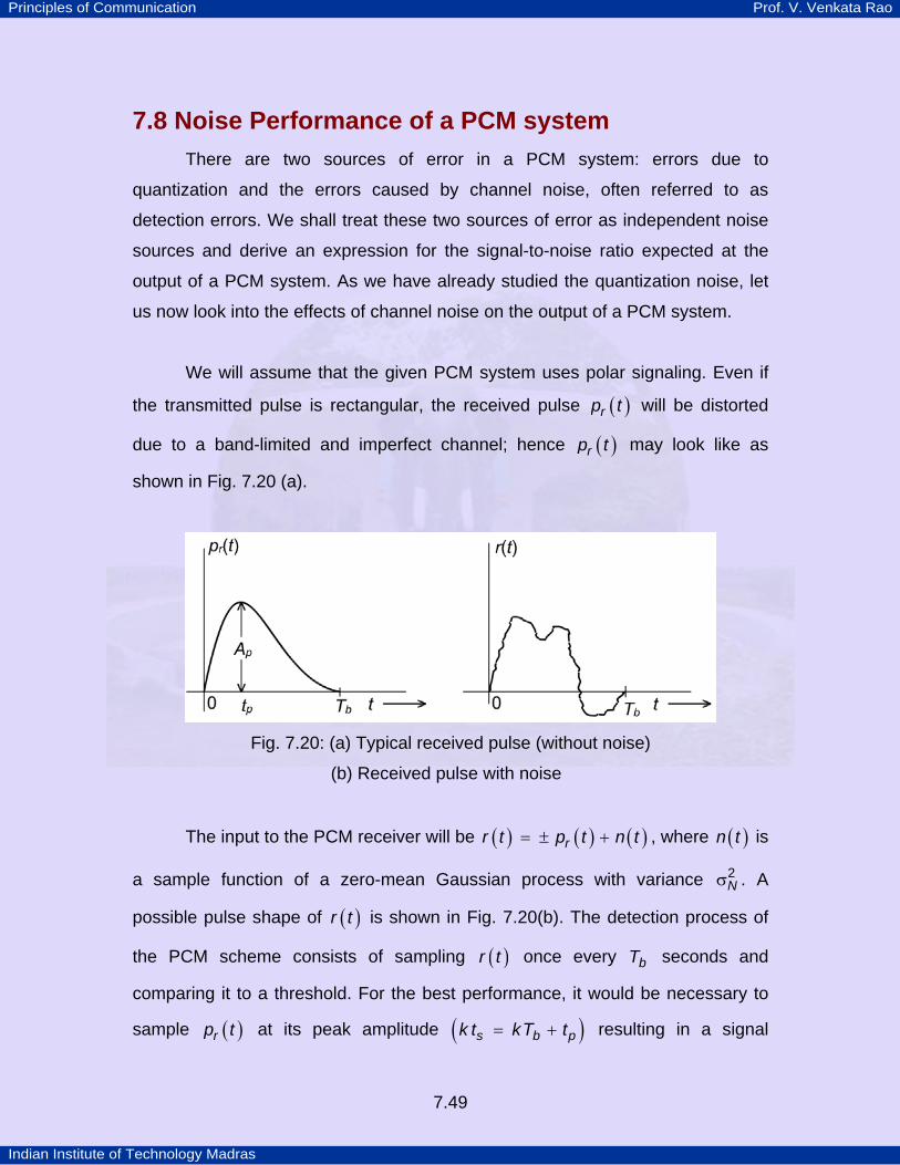
We will assume that the given PCM system uses polar signaling. Even if
the transmitted pulse is rectangular, the received pulse ( )rp t will be distorted
due to a band-limited and imperfect channel; hence ( )rp t may look like as
shown in Fig. 7.20 (a).
Fig. 7.20: (a) Typical received pulse (without noise)
(b) Received pulse with noise
The input to the PCM receiver will be ( ) ( ) ( )rr t p t n t= ± + , where ( )n t is
a sample function of a zero-mean Gaussian process with variance N2σ . A
possible pulse shape of ( )r t is shown in Fig. 7.20(b). The detection process of
the PCM scheme consists of sampling ( )r t once every bT seconds and
comparing it to a threshold. For the best performance, it would be necessary to
sample ( )rp t at its peak amplitude ( )s b pk t kT t= + resulting in a signal

Principles of Communication Prof. V. Venkata Rao
Indian Institute of Technology Madras
7.50
component of pA± . Hence ( )s pr k t A N= ± + whose N is a zero mean
Gaussian variable, representing the noise sample of a band-limited white
Gaussian process with a bandwidth greater than or equal to the bandwidth of the
PCM signal. If binary '1' corresponds to pA+ and '0' to pA− , then,
( )Rf r '1' transmitted is ( )p NN A 2, σ and
( )Rf r '0 ' transmitted is ( )p NN A 2,− σ
where R (as a subscript) represents the received random variable. We assume
that 1's and 0's are equally likely to be transmitted. The above conditional
densities are shown in Fig. 7.21. As can be seen from the figure, the optimum
decision threshold is zero. Let eP ,0 denote the probability of wrong decision,
given that '0' is transmitted (area hatched in red); similarly eP ,1 (area hatched in
blue). Then eP , the probability of error is given by e e eP P P,0 ,11 12 2
= + .
From Fig. 7.21, we have
( ) pe R
N
AP f r d r Q,0
0'0'
∞ ⎛ ⎞= = ⎜ ⎟σ⎝ ⎠∫
Fig. 7.21: Conditional PDFs at the detector input
Similarly pe
N
AP Q,1
⎛ ⎞= ⎜ ⎟σ⎝ ⎠
, which implies

Principles of Communication Prof. V. Venkata Rao
Indian Institute of Technology Madras
7.51
pe
N
AP Q
⎛ ⎞= ⎜ ⎟σ⎝ ⎠
(7.42)
For optimum results, the receiver uses a matched filter whose output is sampled
once every bT seconds, at the appropriate time instants so as to obtain the best
possible signal-to-noise ratio at the filter output. In such a situation, it can be
shown that we can replace p
N
A⎛ ⎞⎜ ⎟σ⎝ ⎠
by bEN0
2 where bE is the energy of the
received binary pulse and N02
represents the spectral height of the, band-limited
white Gaussian noise process. Using the above value for p
N
A⎛ ⎞⎜ ⎟σ⎝ ⎠
yields,
be
EP QN0
2⎛ ⎞= ⎜ ⎟⎜ ⎟
⎝ ⎠ (7.43)
Assuming that there are R binary pulses per sample and W2 samples/second,
we have ( )
=bTRW1
2 where bT represents the duration of each pulse. Hence
the received signal power rS is given by, = =br b
b
ES RW E
T2 or = r
bSERW2
.
Therefore Eq. 7.43 can also be written as
⎛ ⎞
= ⎜ ⎟⎜ ⎟⎝ ⎠
re
SP QRW N0
⎛ ⎞γ
= ⎜ ⎟⎜ ⎟⎝ ⎠
QR
(7.44)
where rSW N0
γ = . Eq. 7.42 to 7.44 specify the probability of any received bit
being in error. In a PCM system, with R bits per sample, error in the
reconstructed sample will depend on which of these R bits are in error. We would
like to have an expression for the variance of the reconstruction error. Assume
the following:
Principles of Communication Prof. V. Venkata Rao
Indian Institute of Technology Madras
7.52
i) The quantizer used is a uniform quantizer
ii) The quantizer output is coded according to natural binary code
iii) eP is small enough so that the probability of two or more errors in a block
of R bits is negligible.
Then, it can be shown that c2σ , the variance of the reconstruction error
due to channel noise is,
( )
( )−
σ =R
p ec R
m P2 22
2
4 2 1
3 2 (7.45)
Details can be found in [3]. In addition to the reconstruction error due to channel
noise, PCM has the inevitable quantization noise with variance Q
22
12∆
σ = , where
∆ = pmL
2 and = RL 2 . Treating these two error sources as independent noise
sources, total reconstruction noise variance e2σ , can be written as
e Q c2 2 2σ = σ + σ
( )−
= +p ep m P Lm
L L
2 22
2 2
4 1
3 3 (7.46)
Let ( ) MM t P2 =
Then, ( ) M
e
PSNR 20 =σ
( )
⎛ ⎞⎜ ⎟=⎜ ⎟+ − ⎝ ⎠
M
pe
PLmP L
2
223
1 4 1 (7.47)
Using Eq. 7.44 in Eq. 7.47, we have
( )( )
⎛ ⎞⎜ ⎟=⎜ ⎟⎛ ⎞γ ⎝ ⎠+ − ⎜ ⎟⎜ ⎟
⎝ ⎠
M
p
PLSNRmL Q
R
2
0 22
3
1 4 1 (7.48)

Principles of Communication Prof. V. Venkata Rao
Indian Institute of Technology Madras
7.53
Figure 7.22 shows the plot of ( )SNR 0 as a function of γ for tone modulation
M
p
Pm2
12
⎛ ⎞⎜ ⎟=⎜ ⎟⎝ ⎠
. However, with suitable modifications, these curves are applicable
even in a more general case.
Fig. 7.22: ( )SNR 0 performance of PCM
Referring to the above figure, we find that when γ is too small, the
channel noise introduces too many detection errors and as such reconstructed
waveform has little resemblance to the transmitted waveform and we encounter
the threshold effect. When γ is sufficiently large, then eP 0→ and e Q2 2σ ≈ σ
which is a constant for a given n . Hence ( )SNR 0 is essentially independent of γ
resulting in saturation.

Principles of Communication Prof. V. Venkata Rao
Indian Institute of Technology Madras
7.54
For the saturation region, ( )SNR 0 can be taken as
( ) ( )⎛ ⎞⎜ ⎟=⎜ ⎟⎝ ⎠
R M
p
PSNRm
20 23 2 (7.49)
The transmission bandwidth PCMB of the PCM system is ( )k WR2 where k is a
constant that is dependent on the signal format used. A few values of k are
given below:
S. No. Signal Format k1 NRZ polar 1
2 RZ polar 2
3 Bipolar (RZ or NRZ) 1
4 Duobinary (NRZ) 12
(For a discussion on duobinary signaling, refer Lathi [3]). As ( )=PCMB k W R2 ,
we have ( )
= PCMBRk W2
. Using this in the expression for ( )SNR 0 in the saturation
region, we obtain
( )PCMBk WM
p
PSNRm20 3 2
⎛ ⎞⎜ ⎟=⎜ ⎟⎝ ⎠
(7.50)
It is clear from Eq. 7.50 that in PCM, ( )SNR 0 increases exponentially with the
transmission bandwidth. Fig. 7.22 also depicts the ( )SNR 0 performance of DSB-
SC and FM ( )2 , 5β = . A comparison of the performance of PCM with that of
FM is appropriate because both the schemes exchange the bandwidth for the
signal -to -noise ratio and they both suffer from threshold phenomenon. In FM,
( )SNR 0 increases as the square of the transmission bandwidth. Hence,
doubling the transmission bandwidth quadruples the output SNR . In the case of

Principles of Communication Prof. V. Venkata Rao
Indian Institute of Technology Madras
7.55
PCM, as can be seen from Eq. 7.49, increasing R by 1 quadruples the output
SNR , where as the bandwidth requirement increases only by R1 . As an
example, if R is increased from 8 to 9, the additional bandwidth is 12.5% of that
required for R = 8. Therefore, in PCM, the exchange of SNR for bandwidth is
much more efficient than that in FM, especially for large values of RTP
1PT. In addition,
as mentioned in the introduction, PCM has other beneficial features such as use
of regenerative repeaters, ease of mixing or multiplexing various types of signals
etc. All these factors put together have made PCM a very important scheme for
modern-day communications.
The PCM performance curves of Fig. 7.22 are based on Eq. 7.48 which is
applicable to polar signaling. By evaluating eP for other signaling techniques
(such as bipolar, duobinary etc.) and using it in Eq. 7.47, we obtain the
corresponding expressions for the ( )SNR 0 . It can be shown that the PCM
performance curves of Fig.7.19 are applicable to bipolar signaling if 3 dB is
added to each value of γ .
Example 7.10 A PCM encoder produces ON-OFF rectangular pulses to represent ‘1’ and
‘0’ respectively at the rate of 1000 pulses/sec. These pulses amplitude modulate
a carrier, ( )c cA tcos ω , where cf 1000>> Hz. Assume that ‘1’s and ‘0’s are
equally likely. Consider the receiver scheme shown in Fig. 7.23.
TP
1PT Note that the FM curve for 2β = and PCM curve for =R 6 intersect at point A . The
corresponding γ is about 30 dB. If we increase γ beyond this value, there is no further
improvement in ( )SNR 0 of the PCM system where as no saturation occurs in FM. If we take
( )T mB f2 1= β + , then the transmission bandwidth requirements of PCM with =R 6 and FM
with 2β = are the same. This argument can be extended to other values of R and β .

Principles of Communication Prof. V. Venkata Rao
Indian Institute of Technology Madras
7.56
Fig. 7.23: Receiver for the Example 7.11
( ) ( )c ts t
2cos , if the input is '1'0 , if the input is '0'
⎧ ω⎪= ⎨⎪⎩
( )w t : sample function of a white Guassian noise process, with a two sided
spectral density of 40.25 10−× Watts/Hz.
BPF : Bandpass filter, centered at cf with a bandwidth of 2 kHz so that the
signal is passed with negligible distortion.
DD : Decision device (comparator)
a) Let Y denote the random variable at the sampler output. Find ( )Yf y0 0
and ( )Yf y1 1 , and sketch them.
b) Assume that the DD implements the rule: if Y 1≥ , then binary ‘1’ is
transmitted, otherwise it is binary ‘0’.
If ( )Yf y1 1 can be well approximated by ( )N 2, 0.1 , let us find the overall
probability of error.
( ) ( ) ( )x t s t n t= + , where ( )n t is the noise output of the BPF.
( ) ( ) ( ) ( ) ( )k c c c s cA t n t t n t tcos cos sin= ω + ω − ω
where kAth
th
2 , if the k transmission bit is '1'
0 , if the k transmission bit is '0'
⎧⎪= ⎨⎪⎩
The random process ( )Y t at the output of the ED, is
( ) ( ) [ ]cY t R t tcos= ω + Θ

Principles of Communication Prof. V. Venkata Rao
Indian Institute of Technology Madras
7.57
( ) ( ) ( ){ }k c sR t A n t n t1
2 2 2⎡ ⎤ ⎡ ⎤= + +⎣ ⎦ ⎣ ⎦
If ‘0’ is transmitted, ( )Y t represents the envelope of narrowband noise. Hence,
the random variable Y obtained by sampling ( )Y t is Rayleigh distributed.
( )yN
Yyf y e y
N
2
020
00 , 0
−= ≥
where ( )N 4 30 0.25 10 4 10 0.1−= × × =
when ‘1’ is transmitted, the random variable Y is Rician, given by
( )y
NY
y yf y I e yN N
2
0
42
1 00 0
21 , 0
⎛ ⎞+− ⎜ ⎟⎜ ⎟⎝ ⎠⎛ ⎞
= ≥⎜ ⎟⎝ ⎠
These are sketched in Fig. 7.24.
Fig. 7.24: The conditional PDFs of Example 7.10
b) As the decision threshold is taken as ‘1’, we have
yeP y e d y e
25 5, 0
110
∞− −= =∫
( )y
eP e d y
2210.2
, 11
2 0.1
−−
− ∞
=π∫
Principles of Communication Prof. V. Venkata Rao
Indian Institute of Technology Madras
7.58
( )Q 10=
( ) eP error P e Q51 102
−⎡ ⎤⎡ ⎤= = + ⎣ ⎦⎣ ⎦

Principles of Communication Prof. V. Venkata Rao
Indian Institute of Technology Madras
7.59
Appendix A7.1 PSD of Noise for Angle Modulated Signals For the case of strong predetection SNR , we have (Eq. 7.22b),
( ) ( ) ( ) ( ) ( )n
c
r tt t t t
Asin ⎡ ⎤θ ϕ + ψ − ϕ⎣ ⎦
Let ( ) ( ) ( ) ( )n
c
r tt t t
Asin ⎡ ⎤λ = ψ − ϕ⎣ ⎦
( ) ( ) ( )j t j tm n
cI e r t e
A1 − ϕ ψ⎡ ⎤= ⎢ ⎥⎣ ⎦
Note that ( )j te ϕ is the complex envelope of the FM signal and ( ) ( )j tnr t e ψ is
( )cen t , the complex envelope of the narrow band noise.
Let ( ) ( ) ( ) ( ) ( )j tce ce c sx t e n t x t j x t− ϕ= = + .
Then, ( ) ( )sc
t x tA1
λ =
We treat ( )cex t to be a sample function of a WSS random process ( )ceX t
where,
( ) ( ) ( ) ( ) ( )j tce ce c sX t e N t X t j X t− Φ= = + (A7.1.1)
Similarly,
( ) ( )sc
t X tA1
Λ = (A7.1.2)
Eq. A7.1.2 implies, the ACF of ( )tΛ , ( )RΛ τ is
( ) ( )sX
cR R
A21
Λ τ = τ (A1.7.3a)
and the PSD
( ) ( )sX
cS f S f
A21
Λ = (A7.1.3b)
We will first show that

Principles of Communication Prof. V. Venkata Rao
Indian Institute of Technology Madras
7.60
( ) ( )ce ceE X t X t 0⎡ ⎤+ τ =⎣ ⎦
( ) ( ) ( ) ( ) ( ) ( )j t tce ce ce ceE X t X t E N t N t e ⎡ ⎤− Φ + τ + Φ⎣ ⎦⎡ ⎤⎡ ⎤+ τ = + τ⎣ ⎦ ⎢ ⎥⎣ ⎦
(A7.4.1a)
( ) ( ) ( ) ( )j t tce ceE N t N t E e− Φ + τ + Φ⎡ ⎤⎡ ⎤= + τ⎣ ⎦ ⎢ ⎥⎣ ⎦
(A7.4.1b)
Eq. A7.4.1(b) is due to the condition that the signal and noise are statistically
independent.
( ) ( ) ( ) ( ) ( ) ( )⎡ ⎤ ⎡ ⎤⎡ ⎤+ τ = τ − τ + τ + τ⎣ ⎦ ⎣ ⎦ ⎣ ⎦c s c s s cce ce N N N N N NE N t N t R R j R R
As ( ) ( )c sN NR Rτ = τ and ( ) ( )
c s s cN N N NR Rτ = − τ ,
we have ( ) ( )⎡ ⎤+ τ =⎣ ⎦ce ceE N t N t 0
Therefore
( ) ( ) ( ) ( ) ( ) ( )c s c s s cce ce X X X X X XE X t X t R R j R R 0⎡ ⎤ ⎡ ⎤⎡ ⎤+ τ = τ − τ + τ + τ =⎣ ⎦ ⎣ ⎦ ⎣ ⎦
This implies ( ) ( )c sX XR Rτ = τ .
Now consider the autocorrelation of ( )ceX t ,
( ) ( ) ( ) ( ) ( ) ( ){ }j t j tce ce ce ceE X t X t E e N t e N t− Φ + τ Φ∗ ∗⎡ ⎤ ⎡ ⎤⎡ ⎤+ τ = + τ⎢ ⎥ ⎢ ⎥⎣ ⎦ ⎣ ⎦ ⎣ ⎦
(A7.1.5)
( ) ( ) ( ) ( ) ( ) ( )j t tce ce ce ce
a j b a j b
E X X E N t N t E e
1 1 2 2
⎡ ⎤Φ − Φ + τ∗ ∗ ⎣ ⎦
+ +
⎡ ⎤⎡ ⎤ ⎡ ⎤= + τ ⎢ ⎥⎣ ⎦ ⎣ ⎦ ⎣ ⎦ (A7.1.6)
( ) ( ) ( ) ( )c s s c c sX X X X X XR R j R R⎡ ⎤ ⎡ ⎤= τ + τ + τ − τ⎣ ⎦ ⎣ ⎦
( ) ( ) ( )s s c c sX X X X XR j R R2 ⎡ ⎤= τ + τ − τ⎣ ⎦
(Note that ( ) ( )c sX XR Rτ = τ as proved earlier.)
( ) ( ) ( )sXR a j b a j b1 1 2 2
1 Re2
⎡ ⎤τ = + +⎣ ⎦

Principles of Communication Prof. V. Venkata Rao
Indian Institute of Technology Madras
7.61
( )a a b b1 2 1 212
= −
Now ( )s cN Nb R1 2 0= τ = for symmetric noise PSD, and ( )
sna R1 2= τ . Hence,
( ) ( ) ( ) ( ){ }( )
s sX N
g
R R E t t1 2 cos2
τ
⎡ ⎤ ⎡ ⎤τ = τ Φ − Φ + τ⎣ ⎦⎣ ⎦
That is,
( ) ( ) ( )s sX NS f S f G f= ∗
where ( ) ( )g G fτ ←⎯→ .
As ( ) ( )sX
cS f S f
A21
Λ = , we have,
( ) ( ) ( )sN
cS f S f G f
A21
Λ ⎡ ⎤= ∗⎣ ⎦
By definition, ( )g τ is the real part of the ACF of ( )j te− Φ . We know that ( )j te Φ is
the complex envelope of the FM process. For a wideband PM or FM, the
bandwidth of ( )G f W>> , the signal bandwidth. The bandwidth of ( )G f is
approximately TB2
, as shown in Fig. A7.1.
Fig. A7.1: Components of ( )S fΛ : (a) typical ( )G f (b) ( )sNS f

Principles of Communication Prof. V. Venkata Rao
Indian Institute of Technology Madras
7.62
Note that ( ) ( ) ( )g G f d f E0 cos 0 1∞
− ∞
⎡ ⎤= = =⎣ ⎦∫ .
For f W≤ , ( ) ( ) ( )sNG f S f N G f d f N0 0
∞
− ∞
∗ =∫ . That is, ( )tΦ is
immaterial as far as PSD of ( )sN t in the range f W≤ is concerned. Hence, we
might as well set ( )t 0ϕ = in the Eq. 7.22 (b), for the purpose of calculating the
noise PSD at the output of the discriminator.

Principles of Communication Prof. V. Venkata Rao
Indian Institute of Technology Madras
7.63
References
1) Herbert Taub and D. L. Shilling, Principles of Communication systems, (2P
ndP
ed.) Mc Graw Hill, 1986
2) Simon Haykin, Communication systems, (4P
thP ed.) John Wiley, 2001
3) B. P. Lathi, Modern digital and analog communication systems, Holt-
Saunders International ed., 1983
Related Documents


