Noise and Jitter Analysis for PLL-Based Frequency …bbs.hwrf.com.cn/downpcbe/8-TP2--Yu_Zhu-7225.pdf · He joined Cadence design Systems in 2005 where he is a ... VCO Macromodeling

DesignCon 2009

Noise and Jitter Analysis for

PLL-Based Frequency

Synthesizer

Yu Zhu, Cadence Design Systems, Inc.

[email protected], (408) 914-6323

Jian Wei Sun, Cadence Design Systems, Inc.

[email protected], (86) 10-82356116

Yuan Zhu Li, Cadence Design Systems, Inc.

[email protected], (408) 473-8467

Dan Feng, Cadence Design Systems, Inc.

[email protected], (408) 944-7733

Helene Thibieroz, Cadence Design Systems, Inc.

[email protected], (512) 342-5369

Abstract

In this article, we present a noise-aware PLL simulation flow. In the flow, we provide a

testbench for each PLL building block, such as VCO, PFD/CP, and FD, where their

voltage-domain models with noise information are extracted to capture their dominant

behaviors. The models are used in the top-level PLL simulation to identify key PLL

characteristics including small signal effects such as noise and jitter, large signal effects

such as locking settle time, and power supply and substrate interference effects. The flow

is tested on an integer-N PLL. We show that the simulation results with the flow closely

match transistor-level analysis while the performance is orders of magnitude faster.

Author(s) Biography

Yu Zhu received his Ph.D. in Electrical Engineering from University of Illinois at

Urbana Champaign in 2002. He currently is a Senior Engineering Manager at Cadence

Design Systems, Inc. His research interests include the computational electromagnetics

and simulation of analog/RF/mixed-signal circuits and systems. He was the recipient of

2001 Y.T.Lo Outstanding Graduate Research Award from University of Illinois. He is a

co-author of the book “Multigrid Finite Element Methods for Electromagnetic Modeling”

by Wiley-IEEE Press.

Jian Wei Sun received his Ph.D in Electrical Engineering from Institute of

Semiconductor, Chinese Academy of Science. He is currently a Member of Consultant

Staff with Cadence Design Systems, Inc. He has previously worked at Lanzhou

University. His research interest is analog and RF circuit simulation.

Yuan Zhu Li received his M.S. degree in Electrical Engineering from Virginia Tech,

Blacksburg, VA, in 2001. He joined Cadence design Systems in 2005 where he is a

Principal Product Engineer focusing on RF Simulation. He spent the first 3 years of his

professional career as RFIC design engineer at RF Integrated Corp, Irvine, CA,

developing WLAN chipset, and 1 year at Tropian Inc, Cupertino, CA as Senior RFIC

Design Engineer designing multi-mode cellular phone chipset.

Dan Feng received his Ph.D in Computer Science from University of Colorado at

Boulder in 1993. He is currently a Senior Architect and Group Director at Cadence

Design Systems, Inc. His research interests are analog/RF and mixed signal simulation.

Helene Thibieroz received her B. Tech. and her M.S. degree from the National Institute

of Applied Sciences, Toulouse, France and her degree in Doctoral studies in Dept. of

Electrical and microelectronics from the Paul Sabatier Scientific University, Toulouse,

France in May, 1995. From 1995 to 2001, she worked as a staff characterization engineer

at Motorola where she focused on Analog characterization for deep submicron CMOS,

RF and BiCmos technologies. Since 2001, she has been working as a staff application

engineer at Cadence Design Systems, where she provides technical support and expertise

on Cadence Analog mixed-signal and RF products.

Introduction

The recent growth in wireless communication has generated high demand for low-cost,

high performance RF frequency synthesizers. The phase-locked loop (PLL) based

frequency synthesizer locks the divided feedback clock from the voltage-controlled

oscillator (VCO) to the reference clock by comparing their phase difference through a

phase-frequency detector (PFD) whose outputs drive the charge pump (CP). The low pass

filter (LPF) at the output of the CP suppresses high frequency components and allows

only the slow-varying DC voltage value to control the VCO frequency. The divide ratio

of the frequency divider (FD) in the PLL is variable so that the output frequency of the

VCO can be set to either an integer or a fractional number, which is an integer-N or

fractional-N frequency synthesizer shown in Fig 1 and 2, respectively.

In the integer-N PLL depicted in Fig 1, the output frequency refout fSPNf )( += . The

channel spacing is equal to the input reference frequency, which limits the loop

bandwidth, and thus causes longer loop settle time for narrow channel spacing and higher

close-in phase noise at the output due to the 1/f noise of VCO. The other problem for the

integer-N PLL is so called reference spurs, since the input reference cannot be filtered

out cleanly by LPF, and it modulates VCO and generates sidebands at .refout nff ±

In contrast, the fractional-N PLL frequency synthesizer can achieve fine frequency

resolution with wider loop bandwidth and relative faster settle time by the periodical

modification of the divider modulus. However the periodicity creates the fractional

spurs at the output. Various methods to suppress the spurs have been proposed. The most

popular one is to dither the divider modulus using a Sigma-Delta modulator (SDM) as

shown in Fig 2, such that the average divide ratio is kFN 2/+ and output frequency is

ref

k

out fFNf )2/( += , where k is the number of bits in the SDM and F is channel

Multi-modulus divider

Modulus control Reset

Counter

P÷

fout

D

U Phase

frequency detector

Charge pump

Lower pass filter

Voltage controlled oscillator

Pre-scalar NN /)1( +÷

Swallower

S÷

Channel Selection

Fig 1. Integer-N PLL Frequency Synthesizer

fref

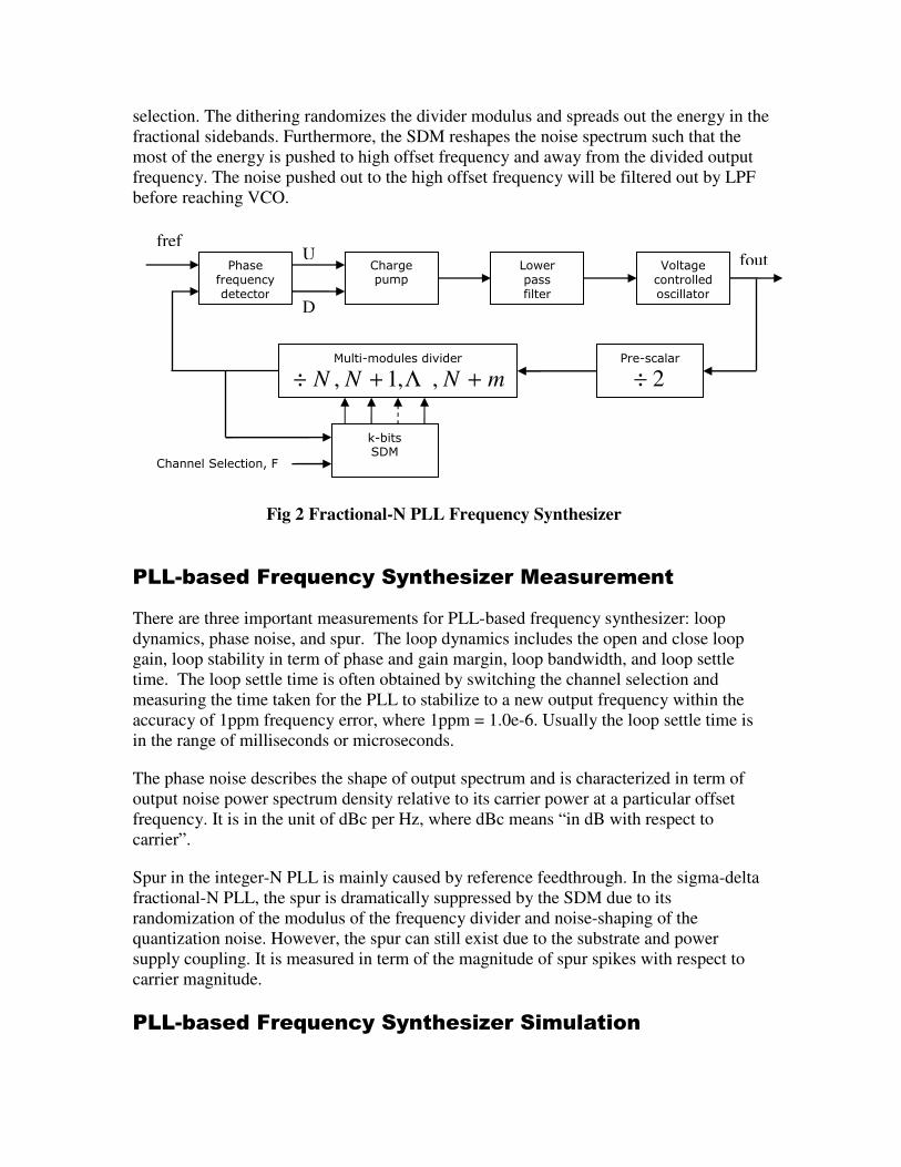
selection. The dithering randomizes the divider modulus and spreads out the energy in the

fractional sidebands. Furthermore, the SDM reshapes the noise spectrum such that the

most of the energy is pushed to high offset frequency and away from the divided output

frequency. The noise pushed out to the high offset frequency will be filtered out by LPF

before reaching VCO.

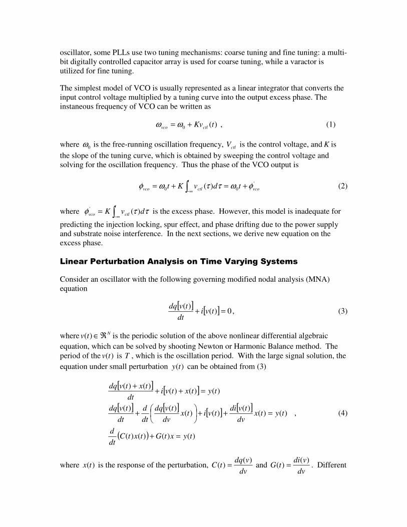
PLL-based Frequency Synthesizer Measurement

There are three important measurements for PLL-based frequency synthesizer: loop

dynamics, phase noise, and spur. The loop dynamics includes the open and close loop

gain, loop stability in term of phase and gain margin, loop bandwidth, and loop settle

time. The loop settle time is often obtained by switching the channel selection and

measuring the time taken for the PLL to stabilize to a new output frequency within the

accuracy of 1ppm frequency error, where 1ppm = 1.0e-6. Usually the loop settle time is

in the range of milliseconds or microseconds.

The phase noise describes the shape of output spectrum and is characterized in term of

output noise power spectrum density relative to its carrier power at a particular offset

frequency. It is in the unit of dBc per Hz, where dBc means “in dB with respect to

carrier”.

Spur in the integer-N PLL is mainly caused by reference feedthrough. In the sigma-delta

fractional-N PLL, the spur is dramatically suppressed by the SDM due to its

randomization of the modulus of the frequency divider and noise-shaping of the

quantization noise. However, the spur can still exist due to the substrate and power

supply coupling. It is measured in term of the magnitude of spur spikes with respect to

carrier magnitude.

PLL-based Frequency Synthesizer Simulation

Multi-modules divider

mNNN ++÷ ,,1, Λ

fout

D

U Phase

frequency detector

Charge pump

Lower pass filter

Voltage controlled oscillator

Pre-scalar

2÷

Channel Selection, F

Fig 2 Fractional-N PLL Frequency Synthesizer

fref

k-bits SDM

It is computationally expensive to simulate PLLs because the period of the VCO is

almost always very short relative to the loop settle time. Transient analysis forces all the

PLL blocks to use the same small time-steps required by the VCO frequency, and the

PLL locking process often involves hundreds of thousands of VCO cycles to reach a

stable state. Hence, the transient analysis of the whole PLL on the transistor-level is very

time-consuming.

The PLL noise analysis is even more challenging. Because PLL generates repetitive

switching events, its noise performance must be evaluated in the presence of its large

signal behavior. Modeling noise as large signals and performing transient analysis with

both signal and noise sources turned on is what is known as "transient noise" analysis,

which requires extremely tight tolerances and small time steps to adequately resolve the

dynamic range difference between noises and signals.

Due to these computational obstacles, PLL noise analysis is usually done by predicting

the noise of individual blocks, building high-level macro-models that exhibit noise, and

simulating the PLL using the models to find the overall noise. Compared with "transient

noise" approach, this method is not only more computationally efficient, but also allows

the identification of the noise contribution from each individual block and guides the

design optimization. However the accuracy of the method depends on the accuracy of the

models of the blocks. There are two different approaches to developing these models:

phase-domain and voltage-domain approach.

In the phase-domain model approach, the models are formulated in terms of the phase of

the signals. This approach requires that the PLL be locked in a steady state and then the

linearized phase-domain model is extracted at the steady state. The phase-domain model

approach is good for determining loop dynamics and for stability analysis.

In the voltage-domain model approach, the models are formulated in terms of the voltage.

This approach does not require a steady state. The nonlinear models generated in this

approach can capture the behavior details of locking and escape process.

The methodology described in this article uses the voltage-domain model approach to

characterize phase-noise, jitter, spur, power supply and substrate noise interference, and

loop settle time characteristics of a PLL. The unique characteristics of the flow described

here are the accurate and automatic model extraction of the dominant behavior of the

main PLL blocks, (such as the VCO, FD and PFD/CP), the translation of their phase-

noise power spectral densities into synchronous or accumulating time-domain noise, and

the integration of the noise behaviors into the voltage-domain macromodels.

VCO Macromodeling

The key component of a PLL is VCO. In PLL-based frequency synthesizers, VCO

usually is a LC cross-coupled differential pair or ring oscillator. The tuning of the LC

oscillator is achieved by MOS varactor while the tuning of the ring oscillator is achieved

by controlling supple voltage to change the inverter threshold. The ring oscillator has

wider tuning range than the LC oscillator. To widen the tuning range of the LC

oscillator, some PLLs use two tuning mechanisms: coarse tuning and fine tuning: a multi-

bit digitally controlled capacitor array is used for coarse tuning, while a varactor is

utilized for fine tuning.

The simplest model of VCO is usually represented as a linear integrator that converts the

input control voltage multiplied by a tuning curve into the output excess phase. The

instaneous frequency of VCO can be written as

)(0 tKvctlvco += ωω , (1)

where 0ω is the free-running oscillation frequency, ctlV is the control voltage, and K is

the slope of the tuning curve, which is obtained by sweeping the control voltage and

solving for the oscillation frequency. Thus the phase of the VCO output is

'

00 )( vco

t

ctlvco tdvKt φωττωφ +=+= ∫ ∞− (2)

where ∫ ∞−=

t

ctlvco dvK ττφ )(' is the excess phase. However, this model is inadequate for

predicting the injection locking, spur effect, and phase drifting due to the power supply

and substrate noise interference. In the next sections, we derive new equation on the

excess phase.

Linear Perturbation Analysis on Time Varying Systems

Consider an oscillator with the following governing modified nodal analysis (MNA)

equation

[ ] [ ] 0)()(

=+ tvidt

tvdq, (3)

where Ntv ℜ∈)( is the periodic solution of the above nonlinear differential algebraic

equation, which can be solved by shooting Newton or Harmonic Balance method. The

period of the )(tv is T , which is the oscillation period. With the large signal solution, the

equation under small perturbation )(ty can be obtained from (3)

[ ] [ ]

[ ] [ ] [ ] [ ]

( ) )()()()(

)()()(

)()()()(

)()()()()(

tyxtGtxtCdt

d

tytxdv

tvditvitx

dv

tvdq

dt

d

dt

tvdq

tytxtvidt

txtvdq

=+

=++

+

=+++

, (4)

where )(tx is the response of the perturbation, dv

vdqtC

)()( = and

dv

vditG

)()( = . Different

from time-invariant system, both )(tG and )(tC are periodic function with period of T .

Eigen-Modes of Linear Time Varying Systems

To better understand the solution to the linearized time-varying system of (4), let us start

with the eigen-mode analysis of (4) and its adjoint system. The adjoint system is

obtained by taking transpose of (4) and replacing dt

d with -

dt

d. Thus we have the

original linear system

( ) 0)()()()( =+ txtGtxtCdt

d , (5)

and its adjoint linear system

0)()()()( =+− txtGtxdt

dtC

TT . (6)

Substitute )()( tuetx R

tRλ−= into (5), where Rλ is referred to as the right eigen-value and

)(tuR is the right periodic eigen-function, we have

( ) )()()()()()( tutCtutGtutCdt

dRRRR λ=+ . (7)

Solution to (7) reveals all the eigen-modes of the original linear system (5). We can write

all the eigen-modes in matrix format:

( ) )()()()()()( tUtCtUtGtUtCdt

dRRRR Λ=+ , (8)

where

=ΛN

R

R

R

λ

λ

Ο

1

, and [ ])()()( 1 tututU N

RRR Λ= . (9)

Similarly, substitute )()( tuetx L

tLλ= into (6), where Lλ is referred to as the left eigen-

value and )(tuL is the left periodic eigen-function, we have

)()()()()()( tutCtutGtudt

dtC L

T

LL

T

L

T λ=+− . (10)

Write all the eigen-solution to (10) in matrix format, we have

( ) )()()()()()( tUtCtUtGtUtCdt

dL

T

LL

T

L

T Λ=+− , (12)

where

=ΛN

L

L

L

λ

λ

Ο

1

, and [ ])()()( 1 tututU N

LLL Λ= . (13)

Multiply (7) with )(tuT

L and (10) with )(tuR and subtract them, we have the equation:

( ) ( ) )()()()()()( tutCtututCtudt

dR

T

LLRR

T

L λλ −= . Therefore, for each right eigenvalue i

Rλ in

the original system, there is a corresponding left eigenvalue i

Lλ in its adjoint system, such

that i

L

i

R λλ = , and their corresponding eigen-functions are consttutCtu R

T

L =)()()( . After

the normalization of eigen-functions, we can write the property of orthogonality in matrix

format:

Λ=Λ=Λ RL , and ItUtCtU R

T

L =)()()( , (14)

where NNI

×ℜ∈ is identity matrix. The eigen-modes of the original and its adjoint

system are ( ))(),(, tutui

L

i

Riλ , where Ni ,,1 Λ= . They are also referred to as Floquet

modes. For a stable linear system, all its eigenvalue should be 0)Re( ≥iλ . In an

autonomous circuit, there exists one eigen-mode whose 0=λ , which can be proven by

taking derivative w.r.t. t on (3)

[ ] [ ]

0)()(

0)()(

0)()(

0)()(

=+

⇒

=+

⇒

=+

⇒=+

dt

dvtG

dt

dvtC

dt

d

dt

dv

dv

vdi

dt

dv

dv

vdq

dt

d

dt

vdi

dt

dv

dv

vdq

dt

dtvi

dt

tvdq

(15)

Comparison with (7) reveals, in an oscillator, the time-derivative of the solution to (3) is

actually the right eigen-function with 0=λ ; while the its corresponding left eigen-

function )(tuL can be solved from (10) with 0=Lλ . In oscillators, the eigen-mode

corresponding to 0=λ does not decay with time and is referred to as the dominant

mode. It is also referred to as the perturbation project vector (PPV). Throughout this

article, we assume the dominant mode is the first eigen-mode and marked as

==

dt

tdvtutu RL

)()(),(,0 111λ (16)

Response on Linear Time Varying Systems

Using the eigen-modes, we can compute the zero-input response to the following

equation:

( )

=⇒

==

=+

−

−

t

t

R

Ne

e

tUtx

xtx

txtGtxtCdt

d

λ

λ

Ο

1

)()(

)0(

0)()()()(

0

Na

a

Μ

1

, (17)

where the coefficients Naa ,,1 Λ are solved by multiplying (17) with )0()0( CU T

L at

0=t and making use of the eigen-mode orthogonality property in (14)

[ ] 01 )0()0(,, xCUaaT

L

T

N =Λ . (18)

Thus the zero-input response is

00 )0()0()()0()0()()(

1

xCUetUxCU

e

e

tUtxT

L

t

R

T

L

t

t

R

N

Λ−

−

−

=

=λ

λ

Ο . (19)

The zero-state response is the solution to the following equation:

( )∫ ∞−

=⇒

==

=+ t

dssysthtx

tx

tytxtGtxtCdt

d

)(),()(

0)0(

)()()()()( , (20)

where ),( sth is the impulse response of linear time-varying system due to an

impulse perturbation at st = , i.e. )()( stty −= δ . Substitute it into (20), integrate

around st = and make use of the zero-input response in (19), we have

( )

)(),()()()(),(

)0(),(

0),()(),()(

)(

)(

)(

1

1

stsUetUsU

e

e

tUsth

Cssh

sthtGsthtCdt

d

T

L

st

R

T

L

st

st

R

N

>=

=

⇒

=

=+

−Λ−

−−

−−

−

λ

λ

Ο

. (21)

The impulse and zero-input response of linear invariant system can be considered a

special case of (19) and (21), where )(tU R and )(tU L are time-invariant constant

functions. However, in the linear periodic time-varying systems, they are periodic

functions with period T .

Non-Linear Perturbation Theory on Autonomous Circuits

So far, we discuss the eigen-modes of the linear time-varying system obtained

through the linearization of the circuit equation at the steady state; and linear

perturbation expansion in term of eigen modes under the condition of 1)( <<tx .

This condition is valid in the perturbation analysis for driven circuits; but not valid

for autonomous circuits.

Let us consider the non-linear perturbation on autonomous circuits. Starting from

the non-linear MNA equation of (3), we inject a perturbation )(ty into the circuit:

[ ] [ ] )()())(()())((

tytxttvidt

txttvdq=+++

++⊥

⊥ αα

(22)

Shown in Fig 3, the response under the perturbation is decomposed into two

components: the phase component )(tα is the phase change along the oscillation

trajectory; while the amplitude component )(tx⊥ is the amplitude change

perpendicular to the oscillation trajectory.

Since we know from (16) the dominant mode in oscillators is the one moving along

the oscillation trajectory, we expand the amplitude component )(tx⊥ using the all the

decaying eigen-modes:

[ ]∑=

⊥

++=+=N

i

N

N

RRi

i

R

tc

tc

ttuttutcttutx2

2

2

)(

)(

))((,)),(()())(()( ΜΛ ααα (23)

Where )(tci are the time-varying expansion coefficients. The amplitude component

is small in magnitude due to the natural consequence of the nonlinear nature of

oscillators that acts to suppress the amplitude variations; hence 1)( <<⊥ tx and it

can be solved using linear perturbation theory.

v 1

v 2

)(tx⊥

))(( ttv α+v N

Fig3. Response to perturbation in oscillators

For the reason of simplicity, we replace )(tt α+ with 't and (22) becomes

[ ] [ ]

[ ] [ ] [ ] [ ]

[ ] [ ] ( )( ) ( ) )(),'('),'(')'(1'

)'(

)(),'()'(

)'(),'()'()'(

)(),'()'(),'()'(

tyttxtGttxtCdt

dtvi

dt

d

dt

tvdq

tyttxdv

tvditvittx

dv

tvdq

dt

d

dt

tvdq

tyttxtvidt

ttxtvdq

=+++

+

=++

+

=+++

⊥⊥

⊥⊥

⊥⊥

α

. (24)

Since [ ] [ ] 0)'(

'

)'(=+ tvi

dt

tvdq, we can simplify the above to the following equation.

[ ] ( )( ) ( )

( )( ) ( ) )(),'('),'(''

)'(

)(),'('),'(''

)'(

'

tyttxtGttxtCttdt

d

dt

dvtC

tyttxtGttxtCdt

d

dt

d

dt

tvdq

t

=+

∂

∂+

∂

∂+

=++

⊥⊥

⊥⊥

α

α

, (25)

where we assume 1/ <<dtdα . We can decompose (25) into two separate

equations about phase and amplitude, respectively. By left multiplying (25) with the

left eigen-function of dominant mode )(1 α+tuT

L and making use the orthogonality

property of (14), we have the equation forα

)()(1 tytudt

d T

L αα

+= , (26)

Where α is related with excess phase '

vcoφ in (2) as απφ 0

'2 fvco = . Assume 1<<α

and perturbation )(ty is slow varying, (26) can be converted to (2).

∫∫ ∞−∞−≈+==

tT

L

t T

Lvco dyufdyuff ττπττατπαπφ )(2)()(22 1

0,0

1

00

' , (27)

where T

Lu1

0, is the DC component of )(1 tuT

L . However, in oscillators, because there

is no restoring force on the phase of a free-running oscillator, the phase-deviation α

due to the perturbation in the direction of the dominant eigenmode accumulates and

becomes large. As a consequence, the assumptions of the linear perturbation theory

do not hold and the phase of the oscillator should be solved in a nonlinear

perturbation model of (26).

The amplitude component )(tx⊥ can be solved by left multiplying (25) with the left

eigen-functions of all the eigen-modes except the dominant mode and making use of

the orthogonality property of (14), we have the equations for its expansion

coefficient )(,),(2 tctc NΛ :

)(

)(

)(

)(

)(

)(

)( 2

222

ty

tu

tu

tc

tc

tcdt

d

tcdt

d

TN

L

T

L

NNN

=

+

ΜΜΟΜ

λ

λ

(28)

The amplitude component is small in magnitude because nonlinearity in oscillators

suppresses the amplitude variations; hence it can be solved using linear perturbation

theory. Ignoring the amplitude deviation due to its small magnitude, the phase is the only

degree of freedom in the autonomous system. The major behavior of the VCO can be

characterized by the order-reduced nonlinear model of (26), which describes the phase

deviation due to the perturbation injected to any node and thus allows for the

characterization of power supply and substrate noise interference.

Noise in Autonomous Circuits

From (21), we can write the transfer function as ),( τth , where st −=τ is the time

interval and (20) becomes

∫ ∞−−=

t

dytthtx τττ )(),()( , (29)

where it is not hard to see from (21), the impulse pulse response ),( τth is periodic

w.r.t. t . ),(),( ττ Tthth += , where T is the period of the system. Taking Fourier

transformation on both sides of (29), we have

∫+∞

∞−= dfefYftHtx

ftj π2)(),()( , and ∑+∞=

−∞=

−−=k

k

k kffYkffHfX )()()( 00 , (30)

where )( fX and )( fY are Fourier transformation of )(tx and )(ty , respectively.

∫+∞

∞−

−= ττ τπ dethftH fj2),(),( and ∫−

−=2/

2/

2),(1

)(

T

T

kftj

k dteftHT

fHπ

. (31)

)( fY

),( τth

)( fX

)()(0 fYfH

)()( 001 ffYffH −−

)2()2( 002 ffYffH −−

)()( 001 ffYffH ++−

)2()2( 002 ffYffH ++−

)(0 fH

)(1 fH−

)(2 fH−

)(1 fH)(2 fH

f

k

Fig 4. Frequency Translation

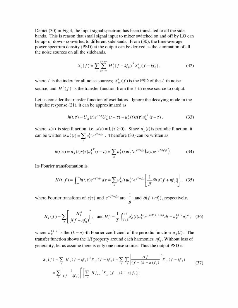
Depict (30) in Fig 4, the input signal spectrum has been translated to all the side-

bands. This is reason that small signal input to mixer switched on and off by LO can

be up- or down- converted to different sidebands. From (30), the time-average

power spectrum density (PSD) at the output can be derived as the summation of all

the noise sources on all the sidebands.

∑ ∑+∞=

−∞=

−−=i

k

k

i

yy

i

kn kffSkffHfS )()()( 0

2

0 , (32)

where i is the index for all noise sources; )( fSi

yy is the PSD of the i -th noise

source; and )( fH i

k is the transfer function from the i -th noise source to output.

Let us consider the transfer function of oscillators. Ignore the decaying mode in the

impulse response (21), it can be approximated as

)()()()()(),( 11 ττττ τ −≈−= Λ− tustutUetUthT

LR

T

LR , (33)

where )(τs is step function, i.e. )0(,1)( ≥= ττs . Since )(1 tuL is periodic function, it

can be written as ∑=n

tnfjn

LL eutu 02,11 )(π . Therefore (33) can be written as

( )∑ −=−≈n

nfjtnfjn

LR

T

LR eseututustuthτππ ττττ 00 22,1111 )()()()()(),( . (34)

Its Fourier transformation is

+⊗== ∑∫

∞+

∞−

− )(1

)(),(),( 0

2,112 0 nffjf

eutudethftHn

tnfjn

LR

fj δττ πτπ , (35)

where Fourier transform of )(τs and τπ 02 nfj

e−

are jf

1 and )( 0nff +δ , respectively.

∑

+=

n

n

k

knffj

HfH

)()(

0

, and n

L

nk

R

T

T

tfnkjn

LR

n

k uudteutuT

H,1,1

2/

2/

)(2,11 0)(1 −

−

−− == ∫π

, (36)

where nk

Ru −,1 is the )( nk − -th Fourier coefficient of the periodic function )(1 tuR . The

transfer function shows the 1/f property around each harmonics 0nf . Without loss of

generality, let us assume there is only one noise source. Thus the output PSD is

∑ ∑

∑ ∑∑

+−

−=

−−−

=−−=

+k

yy

n

n

nk

k

yy

n

n

k

k

yykn

fnkfSHkff

kffSfnkf

HkffSkffHfS

))(()(

1

)())((

)()()(

0

22

0

0

2

0

0

2

0

(37)

If we assume the noise sources consist of white and flicker noise, the output noise PSD

around the k -th harmonics has the form of

∆+

∆=

32)(

f

b

f

afS n

, (38)

where 0kfff −=∆ is the offset frequency.

Combined with noise and signal, the output at the k -th harmonics is )()2cos( 0 tntkfAk +π .

Assume noise magnitude is small, it can be written as ( ))(2cos 0 ttkfAk φπ + , where

)2sin()()( 0tkftAtn k πφ−= . Therefore, the PSD for )(tφ can be derived from (38) as

+==

3222

22)(

f

b

f

a

AS

AfS

k

n

k

φ (39)

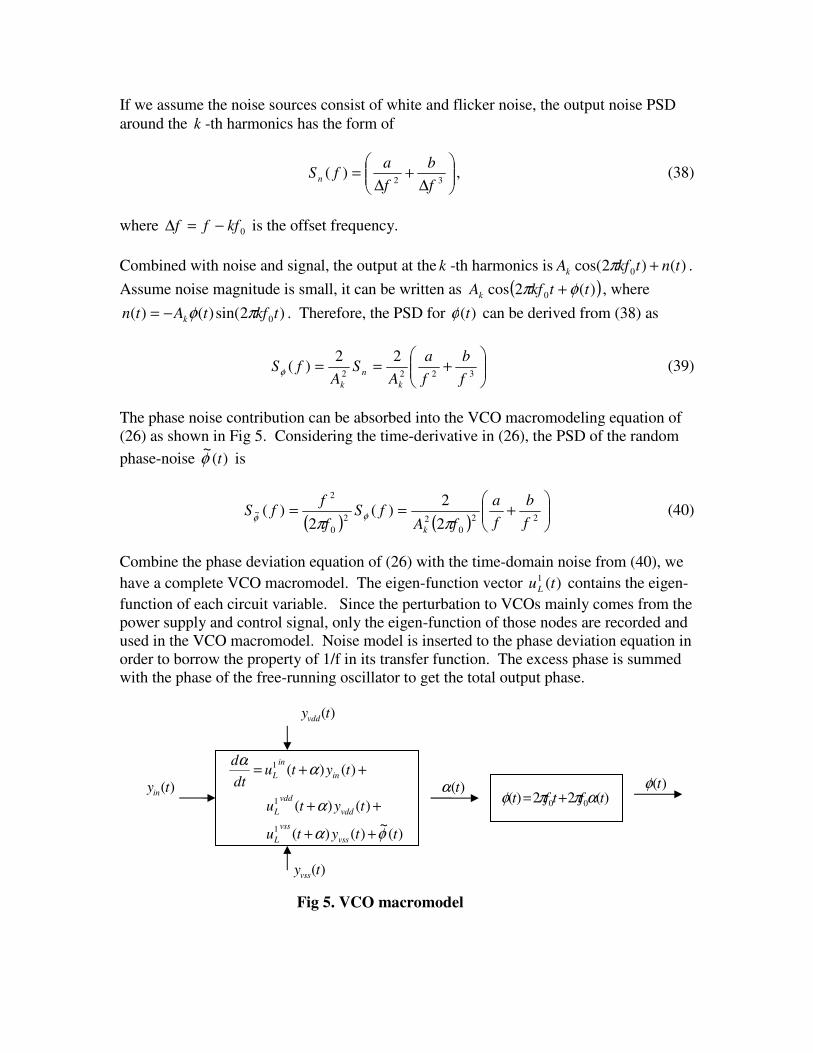
The phase noise contribution can be absorbed into the VCO macromodeling equation of

(26) as shown in Fig 5. Considering the time-derivative in (26), the PSD of the random

phase-noise )(~

tφ is

( ) ( )

+==

22

0

22

0

2

~

2

2)(

2)(

f

b

f

a

fAfS

f

ffS

k ππφφ

(40)

Combine the phase deviation equation of (26) with the time-domain noise from (40), we

have a complete VCO macromodel. The eigen-function vector )(1 tuL contains the eigen-

function of each circuit variable. Since the perturbation to VCOs mainly comes from the

power supply and control signal, only the eigen-function of those nodes are recorded and

used in the VCO macromodel. Noise model is inserted to the phase deviation equation in

order to borrow the property of 1/f in its transfer function. The excess phase is summed

with the phase of the free-running oscillator to get the total output phase.

)(tyin

)(tyvss

)(tyvdd

)(tα)(22)( 00 tftft αππφ +=

)(~

)()(

)()(

)()(

1

1

1

ttytu

tytu

tytudt

d

vss

vss

L

vdd

vdd

L

in

in

L

φα

α

αα

++

++

++=)(tφ

Fig 5. VCO macromodel

VCO Testbench

In order to help with the VCO macromodel extraction, SpectreRF® provides the VCO

testbench shown in Fig 6. The transistor level design of the VCO can be inserted in this

testbench. The testbench provides the terminal for vtune, vdd, and vss. SpectreRF®

performs the several simulations on the testbench:

1. Use periodic steady state analysis to solve for )(tv in (3)

2. Solve for the dominant eigen-mode

==

dt

tdvtutu RL

)()(),(,0

111λ in (8) and (10).

Since )(1 tuR is obtained by taking time-derivative of )(tv , we only solve for )(1 tuL .

3. Periodic noise analysis uses (37) to obtain voltage noise and (39) phase-noise.

4. Create VCO macromodel shown in Fig. 5.

As an example, we extract VCO macromodel for a CMOS differential LC oscillator

shown in Fig 7. In Fig 8, the phase-noise simulation using (37) is depicted as black solid line; the phase-noise from the transient analysis of the VCO macromodel is blue dashed

line; and as a reference, the phase-noise from the transient noise analysis of the transistor-

level VCO is plotted as a red dash-dot line.

The center frequency is 2.48GHz. Below 100KHz, phase-noises are dominated by 1/f

noise and curves show -30dB/dec slope; beyond 100KHz, curves show -20dB/dec slope

since white noise takes over. The close match between the phase-noise from transient

analysis of VCO macromodel and the one from transient analysis of transistor-level VCO

with device noise turned on confirms that the VCO can be replaced by its macromodel in

the PLL simulation without any loss of accuracy.

Fig 6. VCO testbench.

Fig 7. VCO circuit.

Fig 8. VCO phase noise

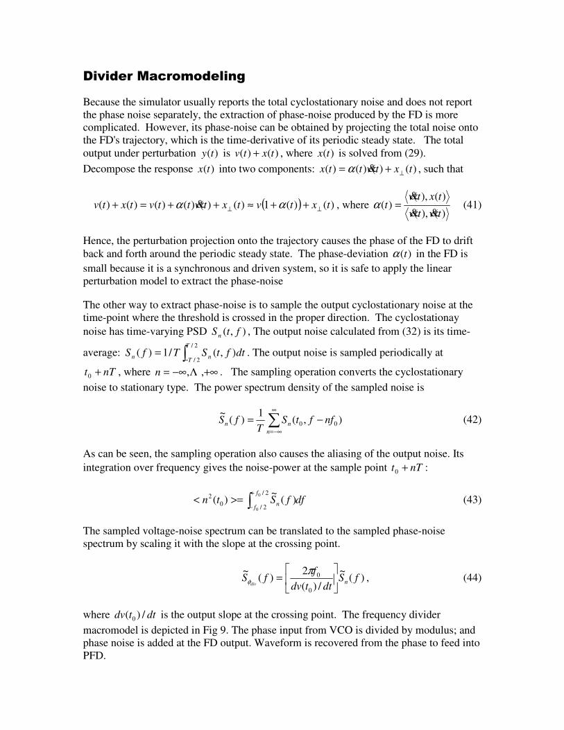
Divider Macromodeling

Because the simulator usually reports the total cyclostationary noise and does not report

the phase noise separately, the extraction of phase-noise produced by the FD is more complicated. However, its phase-noise can be obtained by projecting the total noise onto

the FD's trajectory, which is the time-derivative of its periodic steady state. The total

output under perturbation )(ty is )()( txtv + , where )(tx is solved from (29).

Decompose the response )(tx into two components: )()()()( txtvttx ⊥+= &α , such that

( ) )()(1)()()()()()( txtvtxtvttvtxtv ⊥⊥ ++≈++=+ αα & , where )(),(

)(),()(

tvtv

txtvt

&&

&=α (41)

Hence, the perturbation projection onto the trajectory causes the phase of the FD to drift

back and forth around the periodic steady state. The phase-deviation )(tα in the FD is

small because it is a synchronous and driven system, so it is safe to apply the linear

perturbation model to extract the phase-noise

The other way to extract phase-noise is to sample the output cyclostationary noise at the

time-point where the threshold is crossed in the proper direction. The cyclostationay

noise has time-varying PSD ),( ftSn , The output noise calculated from (32) is its time-

average: ∫−=2/

2/),(/1)(

T

Tnn dtftSTfS . The output noise is sampled periodically at

nTt +0 , where +∞−∞= ,,Λn . The sampling operation converts the cyclostationary

noise to stationary type. The power spectrum density of the sampled noise is

∑∞

−∞=

−=n

nn nfftST

fS ),(1

)(~

00 (42)

As can be seen, the sampling operation also causes the aliasing of the output noise. Its

integration over frequency gives the noise-power at the sample point nTt +0 :

dffStnf

fn∫

+

−>=<

2/

2/0

2 0

0

)(~

)( (43)

The sampled voltage-noise spectrum can be translated to the sampled phase-noise

spectrum by scaling it with the slope at the crossing point.

)(~

/)(

2)(

~

0

0 fSdttdv

ffS ndiv

=

πφ , (44)

where dttdv /)( 0 is the output slope at the crossing point. The frequency divider

macromodel is depicted in Fig 9. The phase input from VCO is divided by modulus; and

phase noise is added at the FD output. Waveform is recovered from the phase to feed into

PFD.

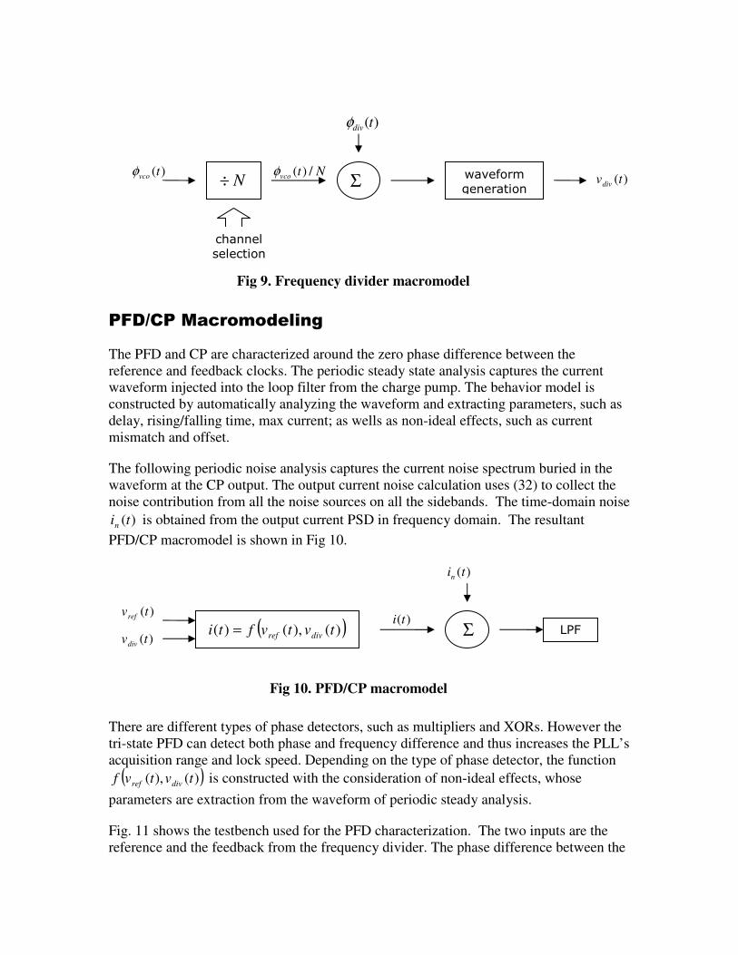
PFD/CP Macromodeling

The PFD and CP are characterized around the zero phase difference between the

reference and feedback clocks. The periodic steady state analysis captures the current

waveform injected into the loop filter from the charge pump. The behavior model is

constructed by automatically analyzing the waveform and extracting parameters, such as

delay, rising/falling time, max current; as wells as non-ideal effects, such as current

mismatch and offset.

The following periodic noise analysis captures the current noise spectrum buried in the

waveform at the CP output. The output current noise calculation uses (32) to collect the

noise contribution from all the noise sources on all the sidebands. The time-domain noise

)(tin is obtained from the output current PSD in frequency domain. The resultant

PFD/CP macromodel is shown in Fig 10.

There are different types of phase detectors, such as multipliers and XORs. However the

tri-state PFD can detect both phase and frequency difference and thus increases the PLL’s

acquisition range and lock speed. Depending on the type of phase detector, the function

( ))(),( tvtvf divref is constructed with the consideration of non-ideal effects, whose

parameters are extraction from the waveform of periodic steady analysis.

Fig. 11 shows the testbench used for the PFD characterization. The two inputs are the

reference and the feedback from the frequency divider. The phase difference between the

Fig 10. PFD/CP macromodel

)(tvref

( ))(),()( tvtvfti divref=)(ti

Σ)(tvdiv

)(tin

LPF

waveform

generation

)(tvcoφN÷

Ntvco /)(φΣ

)(tdivφ

)(tvdiv

channel

selection

Fig 9. Frequency divider macromodel

two inputs is swept around the zero. The load is a voltage source to emulate the effect of

the LPF. Fig 12 is a schematic view of a transistor-level PFD/CP inserted in the

testbench. It consists of two CMOS edge-triggered resettable D flipflops.

The steady state waveform and output current noise spectrum is show in Fig 13. In the

PFD, the AND gate activates the reset of the two D fliplops and thus the U and D net are

simultaneously high for a short period of time given by the delay of AND and flipflops.

The frequency of both inputs is 1MHz. Because the frequency translation in the noise

collection from different sidebands as shown in (32), the output noise shows the spikes at

each harmonics of 1MHz due to the frequency translation of 1/f noise.

Fig 11. PFD/CP testbench.

Fig 12. PFD/CP circuit

PLL Simulation

After the extraction of macromodel for VCO, FD, and PFD/CP, they are inserted in the

integer-N PLL testbench as shown in Fig 14. The divide ratio for FD is preset in the

combined VCO/FD macromodel for integer-N PLLs. The testbench for fractional-N

PLLs has similar layout except that it includes a Verilog-A behavior model implemented

for a dithered MASH sigma delta modulator.

Fig 13. (a) PFD/CP steady state, (b) output noise.

Fig 14. Integer-N PLL testbench.

The locking behavior can be observed by plotting the waveform at the VCO control net,

vtune. The waveforms at vtune from transient analysis of PLL macromodel and transient

analysis of transistor-level PLL are plotted in Fig 15. The two waveforms overlap and

output frequency settles to 2.48GHz. The transient analysis of PLL macromodels takes

only minutes and is hundreds of times faster than the transistor-level PLL simulation.

By turning on the noise in the macromodel of each block, we can simulate the phase-

noise and jitter behaviors of the PLL. While the phase-noise is the power spectrum

density at the PLL output (osc_p and osc_n), the jitter is defined as undesired

perturbation in the timing of the events. The commonly-used jitter in PLL is the referred

to as period jitter, which is defined as the standard deviation of the output period,

)var( 1 ii ttJ −= + , where it is the time of events, such as the threshold crossing.

In Fig 16, we compare the output spectrum from PLL macromodels and transistor-level

PLL, their noise spectrum and jitter value are very close, and predict the reference spurs

correctly. However the noise simulation of PLL macromodels takes only around 30mins;

while the transient noise analysis of transistor-level PLL takes several days.

Injecting a sinusoidal perturbation of 1mV magnitude at 4.7GHz into VCO’s vdd, we

should observe the spurs at ( nm 48.27.4 + )GHz and two strong spurs are located at 260M

and 520MHz plotted in Fig 16. For the purpose of comparison, we also plot the open

loop VCO phase-noise in black dotted line, which shows the noise below 40KHz is

filtered out due to the high-pass transfer function as VCO’s noise appears at the output.

Fig 15. Locking behavior.

Conclusion

In this article, we present a noise-aware PLL simulation methodology implemented in

SpectreRF®. We introduce various PLL simulation methods with the focus on the

voltage-domain model; and discuss the transistor-level simulation and model extraction

for each blocks, such as the VCO, the PFD/CP, and the FD. Floquet theory and eigen-

analysis is used to extract the eigenmodes; the amplitude and phase-components are

separated using the extracted eigen-modes as basis functions; and perturbation analysis is

applied to derive their corresponding equations. The periodic noise analysis is discussed

for each blocks, and their power spectrum densities are translated to time-domain noise

and included in their voltage domain models used in the top-level PLL simulation to

characterize the noise, jitter, interference, and locking behavior.

Reference:

J.L. Stensby. Phase-locked loops: Theory and applicaions. CRC Press, New York, 1997.

B. Razavi. RF Microelectronics. Prentice Hall, NJ 1998.

Fig 16. PLL phase noise and spurs.

K. Kundert. Predicting the Phase Noie and Jittr of PLL Based Frequency Synthesizers.

www.designers-guide.com, 2002

A. Denmir, A. Mehrotra, and J. Roychowdhury. Phase noise in oscillators: a unifying

theory and numerical methods for characterization. IEEE Tras. Circits and Systems. I:

Fundamental Theory and Aplications, 47(5):655-674, May 2000.

A. Demir and J. Roychowdhury. A reliable and efficient procedure for oscillator ppv

computation, with phase noise macromodelling application. IEEE Trans. Computer-

Aided Design of Integrated Circuits and Systes, 22(2):188-197, February 2003.

X. Lai, Y. Wan, and J. Roychowdhury. Fast pll simulation using nonlinear VCO

macromodels for accurate prediction of jitter and cycleslipping due to loop non-idealities

and supply noise. Proc IEEE Asia Souh-Pacifi Design Automatio Confrence, January

2005.

FX Kaertner. Analysis of white and f- noise in oscillators. Interational Journal of Circuit

Theory and. Application, 18:485-519, 1990.