NODE FAILURE TIME AND COVERAGE LOSS TIME ANALYSIS FOR MAXIMUM STABILITY VS MINIMUM DISTANCE SPANNING TREE BASED DATA GATHERING IN MOBILE SENSOR NETWORKS

International Journal of Computer Networks & Communications (IJCNC) Vol.5, No.4, July 2013

DOI : 10.5121/ijcnc.2013.5402 15

NODE FAILURE TIME AND COVERAGE LOSS TIMEANALYSIS FOR MAXIMUM STABILITY VS MINIMUM

DISTANCE SPANNING TREE BASED DATAGATHERING IN MOBILE SENSOR NETWORKS

1Natarajan Meghanathan and 2Philip D. Mumford1Jackson State University, 1400 Lynch St, Jackson, MS, USA

2Air Force Research Lab, Sensors Directorate, Wright Patterson AFB, OH, USA1Corresponding Author E-mail: [email protected]

ABSTRACT

A mobile sensor network is a wireless network of sensor nodes that move arbitrarily. In this paper, weexplore the use of a maximum stability spanning tree-based data gathering (Max.Stability-DG) algorithmand a minimum-distance spanning tree-based data gathering (MST-DG) algorithm for mobile sensornetworks. We analyze the impact of these two algorithms on the node failure times and the resultingcoverage loss due to node failures. Both the Max.Stability-DG and MST-DG algorithms are based on agreedy strategy of determining a data gathering tree when one is needed and using that tree as long as itexists. The Max.Stability-DG algorithm assumes the availability of the complete knowledge of futuretopology changes and determines a data gathering tree whose corresponding spanning tree would exist forthe longest time since the current time instant; whereas, the MST-DG algorithm determines a datagathering tree whose corresponding spanning tree is the minimum distance tree at the current time instant.We observe the Max.Stability-DG trees to incur a longer network lifetime (time of disconnection of thenetwork of live sensor nodes due to node failures), a larger coverage loss time for a particular fraction ofloss of coverage as well as a lower fraction of coverage loss at any time. The tradeoff is that theMax.Stability-DG trees incur a lower node lifetime (the time of first node failure) due to repeated use of adata gathering tree for a longer time.

KEYWORDS

Data Gathering, Maximum Stability, Minimum Distance Spanning Tree, Mobile Sensor Networks, NodeLifetime, Network Lifetime, Coverage Loss Time

1. INTRODUCTION

A mobile sensor network is a dynamically changing wireless distributed system of arbitrarilymoving sensor nodes that operate under limited battery charge, memory and processing capacity.In addition, the bandwidth of these networks is also limited as well as the transmission range ofthe nodes is restricted to conserve the battery charge and to reduce collisions. With all of theabove operating constraints, it is not a practically feasible solution to expect each of these sensornodes to individually transmit their data (directly or through multi-hop route) to the controlcenter, commonly called sink, which is typically located far away from the network field beingmonitored. In this context, several data gathering algorithms that focus on aggregating data fromthe individual sensor nodes through the use of a communication topology (like chain [1], cluster[2], tree [3], connected dominating set [4], and etc) have been proposed. However, almost all ofthese algorithms have been proposed for static sensor networks in which the sensor nodes havebeen assumed to remain fixed at a particular location for the entire lifetime.

mailto:[email protected]


16

The common objective of many of the data gathering algorithms for the static sensor networkshas been to conserve energy and maximize the node lifetime and network lifetime. In this context,in a recent research [5], we evaluated the performance of the data gathering algorithms based ondifferent communication topologies and observed the minimum distance-spanning tree based datagathering (MST-DG) trees to be the most energy-efficient. However, with mobility, the networktopology changes dynamically with time and thus, there is a need to determine stable datagathering trees that do not break frequently. To the best of our knowledge, we have not comeacross any algorithm (centralized or distributed) for stable data gathering in mobile sensornetworks.

In the first half of the paper, we propose a benchmarking algorithm for maximum stability datagathering (Max.Stability-DG) in mobile sensor networks such that the number of tree discoveriesis the global minimum. Given the complete knowledge of the future topology changes, theMax.Stability-DG algorithm operates based on the following greedy principle: Whenever a datagathering tree is required at time instant t, choose the longest-living data gathering tree from t.The above strategy is repeated over the duration of the data gathering session. The sequence ofsuch longest-living data gathering trees incurs the minimum number of tree discoveries. Theworst-case run-time complexity of the Max.Stability-DG tree algorithm is O(n2Tlogn) andO(n3Tlogn) when operated under sufficient-energy and energy-constrained scenarios respectively,where n is the number of nodes in the network and T is the total number of rounds of datagathering; O(n2logn) is the worst-case run-time complexity of the minimum-weight spanning treealgorithm (we use Prim’s algorithm [6]) used to determine the underlying spanning trees fromwhich the data gathering trees are derived. A similar approach is adopted to determine thesequence of MST-DG trees – with the only difference being that the underlying spanning tree is aminimum distance spanning tree determined based on the local network topology and not at thefuture topology changes.

In the second half of the paper, we conduct an exhaustive simulation study of the Max.Stability-DG trees vs. the MST-DG trees and analyze their impact on the node lifetime, network lifetimeand coverage loss time. To the best of our knowledge, we could not find any such comprehensiveanalysis of two data gathering strategies for mobile sensor networks and also with respect to thenode failure times beyond the first node failure as well as analysis on the coverage loss time andfraction of coverage loss at any time due to node failures. The rest of the paper is organized asfollows: Section 2 presents the algorithms to determine the Max.Stability-DG trees and MST-DGtrees. Section 3 presents the simulation environment used and introduces the performance metrics.Section 4 describes the simulation results observed for the node and network lifetime. Section 5describes the simulation results obtained for the coverage loss time and fraction of loss ofcoverage. Section 6 concludes the paper.

2. DATA GATHERING ALGORITHMS BASED ON MAXIMUM STABILITY AND

MINIMUM DISTANCE SPANNING TREES

The system model adopted in this research is as follows: Each sensor node is assumed to operatewith an identical and fixed transmission range. For the purpose of calculating the coverage loss,we also use the sensing range of a sensor node, considered in this research, as half thetransmission range of the node. Basically, a sensor node can monitor and collect data at locationswithin the radius of its sensing range and transmit them to nodes within the radius of itstransmission range. It has been proven in the literature [7] that the transmission range per nodehas to be at least twice the sensing range of the nodes to ensure that coverage impliesconnectivity. Data gathering proceeds in rounds. During a round of data gathering, data getsaggregated starting from the leaf nodes of the tree and propagates all the way to the leader node.


17

An intermediate node in the tree collects the aggregated data from its immediate child nodes andfurther aggregates with its own data before forwarding to its immediate parent node in the tree.We use the notions of static graphs and mobile graphs (adapted from [8]) to capture the sequenceof topological changes in the network and determine a stable data gathering tree that spans overseveral time instants. A static graph is a snapshot of the network at any particular time instant andis modeled as a unit disk graph [9] wherein there exists a link between any two nodes if and onlyif the physical distance between the two end nodes of the link is less than or equal to thetransmission range. The weight of an edge on a static graph is the Euclidean distance between thetwo end nodes of the edge. The Euclidean distance for a link i – j between two nodes i and j,

currently at (Xi, Yi) and (Xj, Yj) is given by: 22 )()( jiji YYXX −+− .

A mobile graph G(i, j), where 1 ≤ i ≤ j ≤ T, where T is the total number of rounds of the datagathering session corresponding to the network lifetime, is defined as Gi ∩ Gi+1 ∩ … Gj. Thus, amobile graph is a logical graph that captures the presence or absence of edges in the individualstatic graphs. In this research work, we sample the network topology periodically for every roundof data gathering to obtain the sequence of static graphs. The weight of an edge in the mobilegraph G(i, j) is the geometric mean of the weights of the edge in the individual static graphsspanning Gi, …, Gj. Since there exist an edge in a mobile graph if and only if the edge exists inthe corresponding individual static graphs, the geometric mean of these Euclidean distanceswould also be within the transmission range of the two end nodes for the entire duration spannedby the mobile graph. Note that at any time, a mobile graph includes only live sensor nodes, nodesthat have positive available energy.

2.1.Maximum Stability Spanning Tree-based Data Gathering (Max.Stability-DG)Algorithm

The Max.Stability-DG algorithm is based on a greedy look-ahead principle and the intersectionstrategy of static graphs. When a mobile data gathering tree is required at a sampling time instantti, the strategy is to find a mobile graph G(i, j) = Gi ∩ Gi+1 ∩ … Gj such that there exists aspanning tree in G(i, j) and no spanning tree exists in G(i, j+1) = Gi ∩ Gi+1 ∩ … Gj ∩ Gj+1. Wefind such an epoch ti, …, tj as follows: Once a mobile graph G(i, j) is constructed with the edgesassigned the weights corresponding to the geometric mean of the weights in the constituent staticgraphs Gi, Gi+1, …, Gj, we run the Prim’s minimum-weight spanning tree algorithm on the mobilegraph G(i, j). If G(i, j) is connected, we will be able to find a spanning tree in it. We repeat theabove procedure until we reach a mobile graph G(i, j+1) in which no spanning tree exists andthere existed a spanning tree in G(i, j). It implies that a spanning tree basically existed in each ofthe static graphs Gi, Gi+1, ..., Gj and we refer to it as the mobile spanning tree for the time instantsti, …, tj. To obtain the corresponding mobile data gathering tree, we choose an arbitrary root nodefor this mobile spanning tree and run the Breadth First Search (BFS) algorithm on it starting fromthe root node. The direction of the edges in the spanning tree and the parent-child relationshipsare set as we traverse its vertices using BFS. The resulting mobile data gathering tree with thechosen root node (as the leader node) is used for every round of data gathering spanning timeinstants ti, …, tj. We then set i = j+1 and repeat the above procedure to find a mobile spanningtree and its corresponding mobile data gathering tree that exists for the maximum amount of timesince tj+1. A sequence of such maximum lifetime (i.e., longest-living) mobile data gathering treesover the timescale T corresponding to the number of rounds of a data gathering session is referredto as the Stable Mobile Data Gathering Tree. Figure 1 presents the pseudo code of theMax.Stability-DG algorithm that takes as input the sequence of static graphs spanning the entireduration of the data gathering session.


18

--------------------------------------------------------------------------------------------------------------------Input: Sequence of static graphs G1, G2, … GT; Total number of rounds of the data gatheringsession – TOutput: Stable-Mobile-DG-TreeAuxiliary Variables: i, jInitialization: i =1; j=1; Stable-Mobile-DG-Tree = Φ

Begin Max.Stability-DG Algorithm

1 while (i ≤ T) do

2 Find a mobile graph G(i, j) = Gi ∩ Gi+1 ∩ … ∩ Gj such that there exists at least onespanning tree in G(i, j) and {no spanning tree exists in G(i, j+1) or j = T}

3 Mobile-Spanning-Tree(i, j) = Prim’s Algorithm ( G(i, j) )

4 Root(i, j) = Choose a node randomly in G(i, j)

5 Mobile-DG-Tree(i, j) = Breadth First Search ( Mobile-Spanning-Tree(i, j), Root(i, j) )

6 Stable-Mobile-DG-Tree = Stable-Mobile-DG-Tree U { Mobile-DG-Tree(i, j) }

7 for each time instant tk ∈{ti, ti+1, …, tj} doUse the Mobile-DG-Tree(i, j) in tk

8 if node failure occurs at tk thenj = k – 1break

end ifend for

9 i = j + 1

10 end while

11 return Stable-Mobile-DG-Tree

End Max.Stability-DG Algorithm--------------------------------------------------------------------------------------------------------------------

Figure 1: Pseudo Code for the Maximum Stability-based Data Gathering Tree Algorithm

While operating the algorithm under energy-constrained scenarios, one or more sensor nodes maydie due to exhaustion of battery charge even though the underlying spanning tree maytopologically exist. For example, if we have determined a data gathering tree spanning acrosstime instants ti to tj using the above approach, and we come across a time instant tk (i ≤ k ≤ j) atwhich a node in the tree fails, we simply restart the Max.Stability-DG algorithm starting fromtime instant tk considering only the live sensor nodes (i.e., the sensor nodes that have positiveavailable energy) and determine the longest-living data gathering tree that spans all the live sensornodes since tk. The pseudo code of the Max.Stability-DG algorithm in Figure 1 handles nodefailures, when run under energy-constrained scenarios, through the if block segment in statement8. If all nodes have sufficient-energy and there are no node failures, the algorithm does notexecute statement 8.

2.2.Minimum Distance Spanning Tree based Data Gathering Algorithm

In our simulation studies (sections 3 through 5), we compare the performance of theMax.Stability-DG trees with that of the minimum-distance spanning tree based data gathering(MST-DG) trees. The sequence of MST-DG trees for the duration of the data gathering session isgenerated as follows: If a MST-DG tree is not known for a particular round, we run the Prim’s


19

minimum-weight spanning tree algorithm on the static graph representing the snapshot of thenetwork topology generated at the time instant corresponding to the round. Since the weights ofthe edges in a static graph represent the physical Euclidean distance between the constituent endnodes of the edges, the Prim’s algorithm will return the minimum-distance spanning tree on thestatic graph. We then choose an arbitrary root node and run the Breadth First Search (BFS)algorithm starting from this node. The MST-DG tree is the rooted form of the minimum-distancespanning tree with the chosen root node as the leader node. We continue to use the MST-DG treeas long as it exists. The leader node of the MST-DG tree remains the same until the tree breaksdue to node mobility or node failures. When the MST-DG tree ceases to exist for a round, werepeat the above procedure. This way, we generate a sequence of MST-DG trees, referred to asthe MST Mobile Data Gathering Tree. The MST-DG algorithm emulates the general strategy(referred to as Least Overhead Routing Approach, LORA [10]) of routing protocols and datagathering algorithms for ad hoc networks and sensor networks. That is, the algorithm chooses adata gathering tree that appears to be the best at the current time instant and continues to use it aslong as it exists. In a recent work [5], we have observed the minimum-distance spanning tree-based data gathering trees to be the most energy-efficient communication topology for datagathering in static sensor networks. To be fair to the Max.Stability-DG algorithm that is proposedand evaluated in this research, the MST-DG algorithm is also run in a centralized fashion with theassumption that the entire static graph information is available at the beginning of each round.

3. SIMULATION ENVIRONMENT AND PERFORMANCE METRICS

We conduct an exhaustive simulation study on the performance of the Max.Stability-DG trees andcompare them with that of the MST-DG trees under diverse conditions of network density andmobility. The simulations are conducted in a discrete-event simulator developed (in Java) by usexclusively for data gathering in mobile sensor networks. The MAC (medium access control)layer is assumed to be collision-free and considered an ideal channel without any interference.Sensor nodes are assumed to be both TDMA (Time Division Multiple Access) and CDMA (CodeDivision Multiple Access)-enabled [11]. Every upstream node broadcasts a time schedule (fordata gathering) to its immediate downstream nodes; a downstream node transmits its data to theupstream node according to this schedule. Such a TDMA-based communication between everyupstream node and its immediate downstream child nodes can occur in parallel, with eachupstream node using a unique CDMA code.

The network dimension is 100m x 100m. The number of nodes in the network is 100 and initially,the nodes are uniform-randomly distributed throughout the network. The sink is located at (50,300), outside the network field. For a given simulation run, the transmission range per sensornode is fixed and is the same across all nodes. The network density is varied by varying thetransmission range per sensor node of 25m (representative of moderate density, with connectivityof 97% and above) and 40m (representative of high density, with 100% connectivity).

Each node is supplied with limited initial energy (2 J per node) and the simulations are conducteduntil the network of live sensor nodes gets disconnected due to the failures of one or more nodes.The energy consumption model used is a first order radio model [12] that has been also used inseveral of the well-known previous work (e.g., [1][2]) in the literature. According to this model,the energy expended by a radio to run the transmitter or receiver circuitry is Eelec = 50 nJ/bit and

∈amp = 100 pJ/bit/m2 for the transmitter amplifier. The radios are turned off when a node wants

to avoid receiving unintended transmissions. The energy lost in transmitting a k-bit message overa distance d is given by: ETX (k, d) = Eelec* k +∈amp *k* d2. The energy lost to receive a k-bit

message is: ERX (k) = Eelec* k.


20

We conduct constant-bit rate data gathering at the rate of 4 rounds per second (one round forevery 0.25 seconds). The size of the data packet is 2000 bits; the size of the control messages usedfor tree discoveries is assumed to be 400 bits. We assume that a tree discovery requires network-wide flooding of the 400-bit control messages such that each sensor node will broadcast themessage exactly once in its neighborhood. As a result, each sensor node will lose energy totransmit the 400-bit message over its entire transmission range and receive the message from eachof its neighbor nodes. In high density networks, the energy lost due to receipt of the redundantcopies of the tree discovery control messages dominates the energy lost at a node for treediscovery. All of these mimic the energy loss observed for flooding-based tree discovery in adhoc and sensor networks.

The node mobility model used is the well-known Random Waypoint mobility model [13] with themaximum node velocity being 3 m/s, 10 m/s and 20 m/s representing scenarios of low, moderateand high mobility respectively. According to this model, each node chooses a random targetlocation to move with a velocity uniform-randomly chosen from [0,…, vmax], and after moving tothe chosen destination location, the node continues to move by randomly choosing another newlocation and a new velocity. Each node continues to move like this, independent of the othernodes and also independent of its mobility history, until the end of the simulation. For a given vmax

value, we also vary the dynamicity of the network by conducting the simulations with a variablenumber of static nodes (out of the 100 nodes) in the network. The values for the number of staticnodes used are: 0 (all nodes are mobile), 20, 50 and 80.We generated 200 mobility profiles of the network for a total duration of 6000 seconds, for everycombination of the maximum node velocity and the number of static nodes. Every data point inthe results presented in Figures 2 through 11 is averaged over these 200 mobility profiles. Theperformance metrics measured in the simulations are:

(i) Node Lifetime – measured as the time of first node failure due to exhaustion of batterycharge.

(ii) Network Lifetime – measured as the time of disconnection of the network of live sensornodes (i.e., the sensor nodes that have positive available battery charge), while the networkwould have stayed connected if all the nodes were alive at that time instant. So, beforeconfirming whether an observed time instant is the network lifetime (at which the network oflive sensor nodes is noticed to be disconnected), we test for connectivity of the underlyingnetwork if all the sensor nodes were alive.We obtain the distribution of node failures as follows: The probability for ‘x’ number of nodefailures (x from ranging from 1 to 100 as we have a total of 100 nodes in our network for allthe simulations) for a given combination of the operating conditions (transmission range pernode, maximum node velocity and number of static nodes) is measured as the number ofmobility profile files that reported x number of node failures divided by 200, which is thetotal number of mobility profiles used for every combination of maximum node velocity andnumber of static nodes. Similarly, we keep track of the time at which ‘x’ (x ranging from 1 to100) number of node failures occurred in each of the 200 mobility profiles for a givencombination of operating conditions and the values for the time of node failures reported inFigures 4, 5 and 6 are an average of these data collected over all the mobility profile files. Wediscuss the results for the distribution of the time and probability of node failures along withthe discussion on node lifetime and network lifetime in Section 4.

(iii) Fraction of Coverage Loss and Coverage Loss Time: If f is denoted as ‘Fraction of CoverageLoss’ (ranging from 0.01 to 1.0, measured in increments of 0.01), the coverage loss time isthe time at which any f randomly chosen locations (X, Y co-ordinates) among 100 locationsin the network is not within the sensing range of any node (explained in more detail below).


21

Since the number of node failures increases monotonically with time and network coveragedepends on the number of live nodes, our assumption in the calculations for network coverageloss is that the fraction of coverage loss increases monotonically with time. We keep track ofthe largest fraction of coverage loss the network has incurred so far, and at the beginning ofeach round we check whether the network has incurred the next largest fraction of coverageloss, referred to as the target fraction of coverage loss. The first time instant during which weobserve the network to have incurred the target coverage loss is recorded as the coverage losstime for the particular fraction of coverage loss, and from then on, we increment the targetcoverage loss by 0.01 and keep testing for the first occurrence of the new target fraction ofcoverage loss in the subsequent rounds. We repeat the above procedure until the networklifetime is encountered for the simulation with the individual data gathering algorithm.

At the beginning of each round, we check for network coverage as follows: We choose 100random locations in the network and find out whether each of these locations is within thesensing range of at least one sensor node. We count the number of locations that are notwithin the sensing range of any node. If the fraction of the number of locations (actualnumber of locations that are not covered / total number of locations considered, which is 100)not within the sensing range of any node equals the target fraction of coverage loss, we recordthe time instant for that particular round of data gathering as the coverage loss timecorresponding to the target fraction of coverage loss. We then increment the target fraction ofcoverage loss by 0.01 and repeat the above procedure to determine the coverage loss timecorresponding to the new incremented value of the target fraction of coverage loss.Each coverage loss time data point reported for particular fractions of coverage loss inFigures 9, 10 and 11 are the average values of the coverage loss times observed when theindividual data gathering tree algorithms are run with the mobility profile files correspondingto a particular condition of network dynamicity (max. node velocity and number of staticnodes) and transmission range per node. The probability for a particular fraction of coverageloss is computed as the ratio of the number of mobility profile files in which thecorresponding fraction of coverage loss was observed divided by the total number of mobilityprofile files (200 mobility profile files for each operating condition).

4. NODE LIFETIME AND NETWORK LIFETIME

We observe a tradeoff between node lifetime and network lifetime for maximum stability vs.minimum-distance spanning tree based data gathering in mobile sensor networks. The MST-DGtrees incur larger node lifetimes (the time of first node failure) for all the 48 operatingcombinations of maximum node velocity, number of static nodes and transmission range pernode. The Max.Stability-DG trees incur larger network lifetime for most of the operatingconditions. The lower node lifetime incurred with the Max.Stability-DG trees is attributed to thecontinued use of stable data gathering trees for a longer time and that too without changing theleader node. It would involve too much of message complexity and energy consumption to havethe sensor nodes coordinate among themselves to choose a leader node for every round. Hence,we choose the leader node for a data gathering tree at the time of discovering it and let the leadernode remain the same for the duration of the tree (i.e., until the tree fails). The same argumentapplies for the continued use of the intermediate nodes that receive aggregate data from one ormore child nodes and transmit them to an upstream node in the tree. Due to the unfairness in nodeusage resulting from the overuse of certain nodes as intermediate nodes and leader node, theMax.Stability-DG trees have been observed to yield a lower node lifetime, especially underoperating conditions (like low and moderate node mobility with moderate and larger transmissionrange per node) that facilitate greater stability.


22

The node lifetime incurred with the Max.Stability-DG trees increases significantly with increasein the maximum node velocity, especially when operated in moderate transmission ranges pernode. We observe an increase in node lifetime by as large as 200-400% as we increase vmax from 3m/s to 10 m/s and operate the nodes at a moderate transmission range of 25m or 30m. A furtherincrease in vmax (i.e., from 10 m/s) to 20 m/s increases the node lifetime further by 50-100%. Wedid not observe an increase in node lifetime when we increase vmax from 3 m/s to 10 m/s at highertransmission ranges per node of 40m. However, a further increase in the maximum node velocityto 20 m/s triggers regular tree failures that contribute to the fairness of node usage, resulting in anincrease in node lifetime by 100-150%. A similar impact of node mobility on the node lifetimeincurred with the MST-DG trees can also be observed, albeit at a lower percentage increase. Weobserve that the node lifetime for the MST-DG trees to increase by about 50-100% as we increasethe maximum node velocity from 3 m/s to 10 m/s. However, a further increase in the maximumnode velocity from 10 m/s to 20 m/s does not create a similar positive impact on the nodelifetime; we observe the node lifetime to further increase by only about 10-20%, and in case oflower transmission ranges per node, we even observe a 5% decrease in node lifetime.

vmax = 3 m/s vmax = 10 m/s vmax = 20 m/s

Figure 2: Average Node and Network Lifetime (Transmission Range per Node = 25 m)

vmax = 3 m/s vmax = 10 m/s vmax = 20 m/s

Figure 3: Average Node and Network Lifetime (Transmission Range per Node = 40 m)

The node lifetime incurred for the MST-DG trees can be larger than that of the Max.Stability-DGtrees by as large as 400% at low and moderate levels of node mobility and by as large as 135% athigher levels of node mobility. For a given level of node mobility, the difference in the nodelifetimes incurred for the MST-DG trees and Max.Stability-DG trees increases with increase inthe transmission range per node (for a fixed number of static nodes) and either remain the same orslightly increase with increase in the number of static nodes (for a fixed transmission range pernode). For a given level of node mobility, the node lifetime incurred with the Max.Stability-DGtrees decreases by about 30-40% as we increase the transmission range per node from 25m to30m, and decreases further by another 50-60% as we increase the transmission range per nodefrom 30m to 40m. The MST-DG trees too suffer a decrease in node lifetime with increase intransmission range per node; but, at a lower scale – due to the relative instability of the trees. Atlarger transmission ranges per node, the data gathering trees are bound to be more stable, and thenegative impact of this on node lifetime is significantly felt in the case of the Max.Stability-DGtrees. For a given transmission range per node, the negative impact associated with the use ofstatic nodes on node lifetime is increasingly observed at vmax values of 3 m/s and 10 m/s. At vmax =20 m/s, since the network topology changes dynamically, even the use of 80 static nodes is notlikely to overuse certain nodes and result in their premature failures. The node lifetime incurredwith MST-DG trees is more impacted with the use of static nodes at low node mobility scenarios


23

(Figure 4) and the node lifetime incurred with the Max.Stability-DG trees is more impacted withthe use of static nodes at moderate and higher node mobility scenarios (Figures 5 and 6).

Transmission Range: 25 m, 0 static nodes Transmission Range: 25 m, 80 static nodes


Figure 4: Distribution of Node Failure Times and Probability of Node Failures [vmax = 3 m/s]




The Max.Stability-DG trees compensate for the premature failures of certain nodes by incurring alower energy loss per round and energy loss per node due to lower tree discoveries and shortertree height with more even distribution of the number of child nodes per intermediate node. Asthe dynamicity of the network increases, the data gathering trees become less stable, and thishelps to rotate the roles of the intermediate nodes and leader node among the nodes to increasethe fairness of node usage. All of these save significantly more energy at the remaining nodes thatwithstand the initial set of failures. As a result, we observe the Max.Stability-DG trees to observea significantly longer network lifetime compared to that of the MST-DG trees. There are onlyfour combinations of operating conditions under which the MST-DG trees incur larger network


24

lifetime – these correspond to transmission range per node of 25m and vmax = 3 m/s (0, 20 and 50static nodes), 20 m/s (0 static nodes).

The difference in the network lifetime incurred for the Max.Stability-DG trees and that of theMST-DG trees increases with increase in the maximum node velocity and transmission range pernode. At low, moderate and high levels of node mobility, the network lifetime incurred with theMax.Stability-DG trees can be larger than that of the MST-DG trees by about 5-20%, 15-40% and20-60% respectively, with the difference increasing with increase in the transmission range pernode. Similar range of differences in the network lifetime can be observed for the two datagathering trees at transmission ranges per node of 25m, 30m and 40m, with the differenceincreasing as the maximum node velocity increases. For a given vmax and transmission range pernode, the number of static nodes does not make a significant impact on the difference in thenetwork lifetime incurred with the two data gathering trees at moderate transmission ranges pernode of 25 and 30m. However, at larger transmission ranges per node of 40m, the difference inthe network lifetime decreases by about 15-35%. This could be attributed to the relatively highstability of the Max.Stability-DG trees when operated at larger transmission ranges per node inthe presence of more static nodes.With respect the impact of the operating parameters on the absolute magnitude of the networklifetime, we observe the network lifetime incurred with the two data gathering trees increaseswith increase in the number of static nodes for a given value of vmax and transmission range pernode. For a given level of node mobility, the network lifetime increases with increase intransmission range per node; however, for the MST-DG trees, the rate of increase decreases withincrease in the maximum node velocity. This could be attributed to the relative instability of theMST-DG trees at high node mobility levels, requiring frequent tree reconfigurations. During anetwork-wide flooding, all nodes in the network tend to lose energy, almost equally. TheMax.Stability-DG trees maintain a steady increase in the network lifetime with increase intransmission range per node for all levels of node mobility. For a given transmission range pernode and number of static nodes, the network lifetime incurred for the two data gathering treesdecreases with increase in the maximum node velocity, especially for the MST-DG trees due totheir instability. This could be attributed to the energy loss incurred due to frequent treediscoveries. The network lifetime incurred with the Max.Stability-DG trees and MST-DG treesdecreases by about 30-50% and 50-100% respectively as we increase the maximum node velocityfrom 3 m/s to 20 m/s for a fixed transmission range per node and number of static nodes.





25

For a given transmission range per node, with the absolute values of the node lifetime increasingwith increase in the maximum node velocity and the network lifetime decreasing with increase inthe maximum node velocity, we observe the maximum increase in the absolute time of nodefailures to occur at low node mobility. This vindicates the impact of network-wide flooding basedtree discoveries on energy consumption at the nodes. Since all nodes are likely to lose the sameamount of energy with flooding, the more we conduct flooding, the larger is the network-wideenergy consumption. As a result, node failures tend to occur more frequently when we conductfrequent flooding. Thus, even though operating the network at moderate and high levels of nodemobility helps us to extend the time of first node failure, the subsequent node failures occur toosoon after the first node failure. This could be justified with the observation of flat curves for theMST-DG trees with respect to the distribution of node failure times (in Figures 4, 5 and 6). Thedistribution of node failure times is relatively steeper for the Max.Stability-DG trees. The unfairusage of nodes in the initial stages does help the Max.Stability-DG trees to prolong the networklifetime. Aided with node mobility, it is possible for certain energy-rich nodes (that might havebeen leaf nodes in an earlier data gathering tree) to keep the network connected for a longer timeby serving as intermediate nodes, and the energy-deficient nodes serve as leaf nodes during thelater rounds of data gathering.The impact of mobility in prolonging node failure lifetimes could also be explained by the lowerprobability of node failure observed for the Max.Stability-DG trees in comparison to the MST-DG trees when there are 0 static nodes (the plots to the left in Figures 4, 5 and 6). At 80 staticnodes, the probability of node failures for the two data gathering trees is about the same and ishigher than that observed when all nodes are mobile. This could be attributed to the repeatedoveruse of certain nodes as intermediate nodes and leader node on relatively more stable datagathering trees. Thus, with the use of static nodes, even though the absolute magnitude of thenetwork lifetime can be marginally increased (by about 10-70%; the increase is larger at moderatetransmission range per node and larger values of vmax), the probability of node failures to occuralso increases.In terms of the percentage difference in the values for the network lifetime and node lifetimeincurred with the two data gathering trees, we observe the Max.Stability-DG trees to incur asignificantly prolonged network lifetime, beyond the time of first node failure. For a giventransmission range per node and maximum node velocity, we observe the difference between thenode lifetime and network lifetime for the Max.Stability-DG trees to increase significantly withincrease in the number of static nodes. This could be attributed to the reduction in the number offlooding-based tree discoveries. For a given level of node mobility, we observe the difference inthe node lifetime and network lifetime for the Max.Stability-DG trees to increase with increase inthe transmission range per node. This could be again attributed to the decrease in the number ofnetwork-wide flooding based tree discoveries when operated at larger transmission ranges pernode. Relatively, the MST-DG trees incur a very minimal increase in the network lifetimecompared to the node lifetime, especially when operated at higher levels of node mobility. Thenetwork lifetime incurred with the Max.Stability-DG trees could be larger than the node lifetimeas low as by a factor of 1.7 and as large as by a factor of 23. On the other hand, the networklifetime incurred with the MST-DG trees could be larger than the node lifetime as low as by afactor of 1.4 and as large as by a factor of 5.7.One can also observe from Figures 4, 5 and 6 that the number of node failures that require for thenode failure time incurred with the Max.Stability-DG trees to exceed that of the node failure timeincurred with the MST-DG trees decreases with increase in maximum node mobility. This couldbe attributed to the premature very early node failure occurring for the Max.Stability-DG treeswhen operated under low node mobility scenarios, with the time of first node failure for the MST-DG tree being as large as 400% more than the time of first node failure for the Max.Stability-DGtree. On the other hand, at high levels of node mobility, the time of first node failure incurred withthe MST-DG trees is at most 100% larger than that of the Max.Stability-DG trees. Hence, the


26

node failure times incurred with the Max.Stability-DG trees could quickly exceed that of theMST-DG trees at higher levels of node mobility. At the same time, the probability for nodefailures to occur (that was relatively low at moderate transmission ranges per node, low andmoderate levels of node mobility) with the Max.Stability-DG trees converges to that of the MST-DG trees when operated at higher levels of node mobility as well as with larger transmissionranges per node. For a given vmax value and transmission range per node, we also observe that thenumber of node failures required for the failure times incurred with the Max.Stability-DG trees toexceed that of the MST-DG trees increases with increase in the number of static nodes.

5. COVERAGE LOSS ANALYSIS5.1 Coverage Loss at a Common Timeline

In this section, we compare the loss of coverage incurred with both the Max.Stability-DG andMST-DG trees with respect to a common timeline, chosen to be the minimum of the networklifetime obtained for the two data gathering trees under every operating condition oftransmission range per node, maximum node velocity and the number of static nodes. Given thenature of the results obtained for the network lifetime under different operating conditions, theminimum of the network lifetime for the two data gathering trees ended up mostly being thenetwork lifetime observed for the MST-DG trees. For this value of network lifetime, we measuredthe fraction of coverage loss in the network incurred for each of the two data gathering trees, aswell as measured the probability with which the corresponding fraction of coverage loss isobserved.

Under the above measurement model, we observe the Max.Stability-DG trees incur lower valuesof the fractions of coverage loss at the minimum of the network lifetime incurred for the two datagathering trees for most of all the 48 combinations of the operating conditions of maximum nodevelocity, number of static nodes and transmission range per node (see Figures 7 and 8). However,the fraction of coverage loss observed for the Max.Stability-DG trees is bound to occur with ahigher probability than that of the coverage loss to be incurred by using the MST-DG trees. Thedifference in the fraction of coverage loss incurred for the Max.Stability-DG trees vis-à-vis couldbe as large as 0.18-0.21, observed at transmission range per node of 40m and 80 static nodes,under all levels of node mobility. The only three combinations of operating conditions for whichthe Max.Stability-DG trees sustain a larger value for the fraction of coverage loss (that too, onlyby 0.02) are at a transmission range per node of 25m - vmax = 3 m/s, 0 and 20 static nodes; and vmax

= 10 m/s, 0 static nodes.

vmax = 3 m/s vmax = 10 m/s vmax = 20 m/sFigure 7: Fraction of Coverage Loss and Associated Probability (Trans. Range/Node = 25 m)

vmax = 3 m/s vmax = 10 m/s vmax = 20 m/sFigure 8: Fraction of Coverage Loss and Associated Probability (Trans. Range/Node = 40 m)


27

In the case of the Max.Stability-DG trees, for a fixed vmax value, we observe the fraction of loss ofcoverage to decrease with increase in transmission range per node from 25m to 40m, of coursewith a higher probability. The significant decrease in the loss of coverage (as low as 0.05) athigher transmission range per node of 40m could also be attributed to the increase in the networklifetime, and also due to the reason that we measure the loss of coverage at a time value(corresponding to the network lifetime of the MST-DG trees), which is lower than the networklifetime of the Max.Stability-DG trees. For fixed vmax and transmission range, as we increase thenumber of static nodes, the fraction of coverage loss decreases significantly for Max.Stability-DGtrees by about 0.05 to 0.1; whereas, the fraction of coverage loss for the MST-DG trees suffers avery minimal decrease or remains the same. For a fixed # static nodes and transmission range pernode, the maximum node velocity has minimal impact on the fraction of coverage loss for theMST-DG trees. However, for the Max.Stability-DG trees, as we increase the maximum nodevelocity from 3 m/s to 20 m/s, at transmission ranges per node of 30m and 40m, the fraction ofcoverage loss that was already low (in the range 0.10 – 0.15 range) decreases further by about0.05 – 0.07.

5.2 Distribution of Coverage Loss

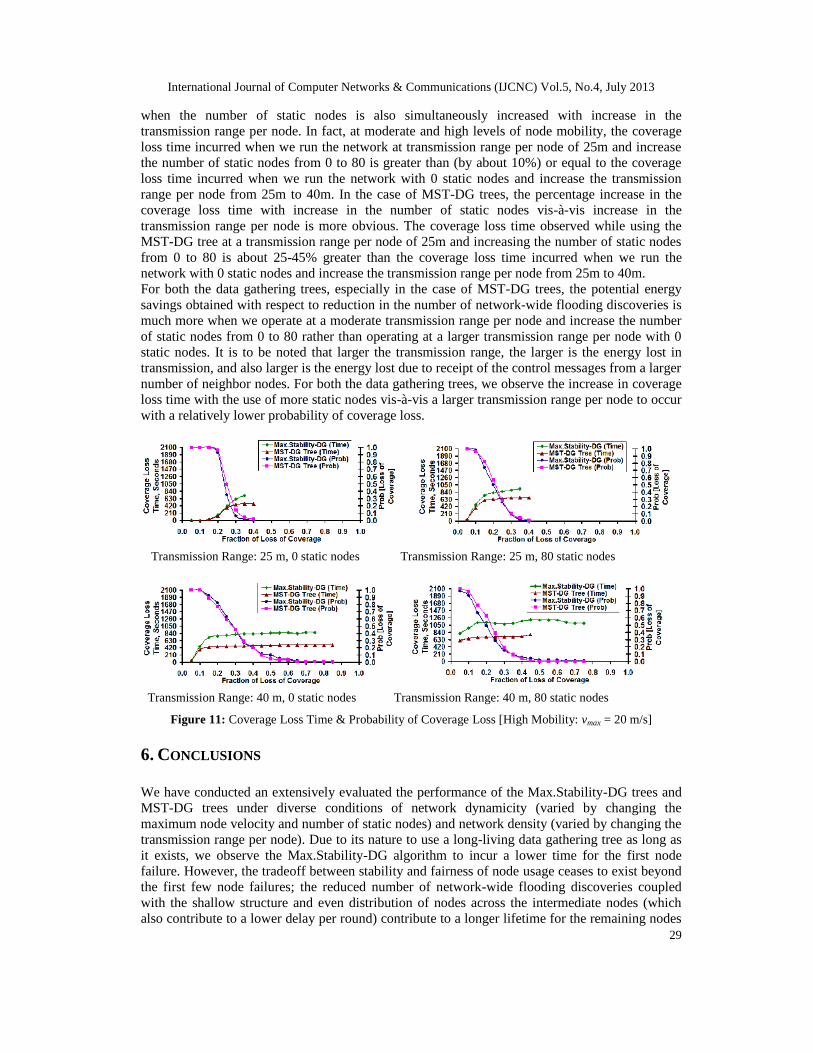
In Figures 9, 10 and 11, we illustrate the distribution of the time (referred to as the coverage losstime) at which particular fractions of coverage loss occurs in the network when run with theMax.Stability-DG and MST-DG trees (until the network lifetime of the individual data gatheringtree). The Max.Stability-DG trees incur larger values of coverage loss time for moderate andhigher values of the fractions of coverage loss (generally above 0.15 or 0.2), under most of thecombinations of the operating conditions of maximum node velocity, 0 and 80 static nodes andtransmission range per node. The only combination of operating conditions for which theMax.Stability-DG trees sustain a lower coverage loss time for fractions of coverage loss greaterthan 0.15-0.2 is at vmax = 3 m/s – transmission ranges per node of 25m. For quantitativecomparison purposes, we base our discussion in this section on the coverage loss time observedwhen the fraction of coverage loss is 0.3. For most of the combinations of operating conditions,we observe the coverage loss times incurred with the Max.Stability-DG and MST-DG trees toflatten out (i.e., not appreciably increase) starting from this fraction of coverage loss.In terms of the percentage difference in the coverage loss time incurred at a fraction of coverageloss of 0.3, we observe the coverage loss time incurred with the Max.Stability-DG trees to beabout 15-40%, 15-45% and 30-70% greater than the coverage loss time incurred with the MST-DG trees at low, moderate and high levels of node mobility respectively. For a fixed transmissionrange per node and number of static nodes, the absolute magnitude for the coverage loss timeincurred for both the data gathering trees decreases with increase in the vmax value. The MST-DGtrees suffer the most with their coverage loss time decreasing by about 20-40% as we increasevmax from 3 m/s to 10 m/s, and a further decrease by another 20-40% as we increase vmax from 10m/s to 20 m/s. The Max.Stability-DG trees suffer a relatively slower decrease in coverage losstime by about 10-25% as we increase vmax from 3 m/s to 10 m/s, and a further decrease by another5-15% as we increase vmax from 10 m/s to 20 m/s. The consolation is that the decrease in thecoverage loss time occurs at a lower probability for the fraction of coverage loss to be at 0.3.To illustrate the immense negative impact of increase in the maximum node velocity on thecoverage loss time for MST-DG trees, we cite the following observation from Figures 9, 10 and11: the coverage loss time incurred with vmax = 3 m/s, transmission range of 25m and 0 staticnodes is even greater than the coverage loss time incurred with vmax = 20 m/s, transmission rangeof 40m and 80 static nodes (by about 5%). Thus, neither the increase in the number of static nodesand nor the increase in the transmission range per node can adequately compensate for thedecrease in the coverage loss time when we increase the maximum velocity of a node from 3 m/sto 20 m/s. On the contrary, for the same conditions, we observe the coverage loss time incurred


28

with the Max.Stability-DG trees at vmax = 20 m/s, transmission range per node of 40m and 80static nodes to be about 70% greater than the coverage loss time incurred at vmax = 3m/s,transmission range of 25m and 0 static nodes. This emphasizes the importance of discoveringstable data gathering trees that can reduce the energy lost due to frequent network-wide floodingat high levels of node mobility and prolong the coverage loss time incurred with the datagathering trees.



Figure 9: Coverage Loss Time and Probability of Coverage Loss [Low Mobility: vmax = 3 m/s]



Figure 10: Coverage Loss Time & Probability of Coverage Loss [Mod. Mobility: vmax = 10 m/s]

For a given level of node mobility, the coverage loss time incurred with the Max.Stability-DGtrees almost doubles, if not more, as we increase the transmission range per node from 25m to40m and the number of static nodes from 0 to 80. This could be attributed to the significantenergy savings obtained as a result of the need for very few network-wide flooding treediscoveries with the use of the Max.Stability-DG algorithm when operated at larger transmissionranges per node and/or more static nodes. We observe significant gains in the coverage loss time


29

when the number of static nodes is also simultaneously increased with increase in thetransmission range per node. In fact, at moderate and high levels of node mobility, the coverageloss time incurred when we run the network at transmission range per node of 25m and increasethe number of static nodes from 0 to 80 is greater than (by about 10%) or equal to the coverageloss time incurred when we run the network with 0 static nodes and increase the transmissionrange per node from 25m to 40m. In the case of MST-DG trees, the percentage increase in thecoverage loss time with increase in the number of static nodes vis-à-vis increase in thetransmission range per node is more obvious. The coverage loss time observed while using theMST-DG tree at a transmission range per node of 25m and increasing the number of static nodesfrom 0 to 80 is about 25-45% greater than the coverage loss time incurred when we run thenetwork with 0 static nodes and increase the transmission range per node from 25m to 40m.For both the data gathering trees, especially in the case of MST-DG trees, the potential energysavings obtained with respect to reduction in the number of network-wide flooding discoveries ismuch more when we operate at a moderate transmission range per node and increase the numberof static nodes from 0 to 80 rather than operating at a larger transmission range per node with 0static nodes. It is to be noted that larger the transmission range, the larger is the energy lost intransmission, and also larger is the energy lost due to receipt of the control messages from a largernumber of neighbor nodes. For both the data gathering trees, we observe the increase in coverageloss time with the use of more static nodes vis-à-vis a larger transmission range per node to occurwith a relatively lower probability of coverage loss.



Figure 11: Coverage Loss Time & Probability of Coverage Loss [High Mobility: vmax = 20 m/s]

6. CONCLUSIONS

We have conducted an extensively evaluated the performance of the Max.Stability-DG trees andMST-DG trees under diverse conditions of network dynamicity (varied by changing themaximum node velocity and number of static nodes) and network density (varied by changing thetransmission range per node). Due to its nature to use a long-living data gathering tree as long asit exists, we observe the Max.Stability-DG algorithm to incur a lower time for the first nodefailure. However, the tradeoff between stability and fairness of node usage ceases to exist beyondthe first few node failures; the reduced number of network-wide flooding discoveries coupledwith the shallow structure and even distribution of nodes across the intermediate nodes (whichalso contribute to a lower delay per round) contribute to a longer lifetime for the remaining nodes


30

in the network and significantly prolong the network lifetime as well as the coverage loss time.On the contrary, the MST-DG trees that incur a larger time for the first node failure are observedto incur a significantly lower network lifetime and lower coverage loss time for a given fractionof loss of coverage (and correspondingly incur a larger fraction of coverage loss at any time),owing to frequent network-wide flooding-based tree discoveries that expedite the node failuresafter the first node failure. We did not come across such a comprehensive analysis for nodefailure times, network lifetime, coverage loss times and fraction of coverage loss in any priorwork in the literature.

ACKNOWLEDGMENTS

This research was sponsored by the U. S. Air Force Office of Scientific Research (AFOSR)through the Summer Faculty Fellowship Program for the lead author (Natarajan Meghanathan) inJune-July 2012. The research was conducted under the supervision of the co-author (Philip D.Mumford) at the U. S. Air Force Research Lab (AFRL), Wright-Patterson Air Force Base(WPAFB) Dayton, OH. The AFRL public release number for this article is 88ABW-2012-4893.The views and conclusions in this document are those of the authors and should not be interpretedas representing the official policies, either expressed or implied, of the funding agency.

REFERENCES[1] S. Lindsey, C. Raghavendra and K. M. Sivalingam, “Data Gathering Algorithms in Sensor Networks

using Energy Metrics,” IEEE Transactions on Parallel and Distributed Systems, 13(9):924-935,September 2002.

[2] W. Heinzelman, A. Chandrakasan and H. Balakarishnan, “Energy-Efficient Communication Protocolsfor Wireless Microsensor Networks,” Proceedings of the Hawaiian International Conference onSystems Science, January 2000.

[3] N. Meghanathan, “An Algorithm to Determine Energy-aware Maximal Leaf Nodes Data GatheringTree for Wireless Sensor Networks,” Journal of Theoretical and Applied Information Technology, ,vol. 15, no. 2, pp. 96-107, May 2010.

[4] N. Meghanathan, “A Data Gathering Algorithm based on Energy-aware Connected Dominating Setsto Minimize Energy Consumption and Maximize Node Lifetime in Wireless Sensor Networks,”International Journal of Interdisciplinary Telecommunications and Networking, vol. 2, no. 3, pp. 1-17,July-September 2010.

[5] N. Meghanathan, “A Comprehensive Review and Performance Analysis of Data GatheringAlgorithms for Wireless Sensor Networks,” International Journal of InterdisciplinaryTelecommunications and Networking, vol. 4, no. 2, pp. 1-29, April-June 2012.

[6] T. H. Cormen, C. E. Leiserson, R. L. Rivest and C. Stein, “Introduction to Algorithms,” 3rd Edition,MIT Press, July 2009.

[7] H. Zhang and J. C. Hou, “Maintaining Sensing Coverage and Connectivity in Large SensorNetworks,” Wireless Ad hoc and Sensor Networks: An International Journal, vol. 1, no. 1-2, pp. 89-123, January 2005.

[8] A. Farago and V. R. Syrotiuk, “MERIT: A Scalable Approach for Protocol Assessment,” MobileNetworks and Applications, Vol. 8, No. 5, pp. 567 – 577, October 2003.

[9] F. Kuhn, T. Moscibroda and R. Wattenhofer, “Unit Disk Graph Approximation,” Proceedings of theWorkshop on Foundations of Mobile Computing, pp. 17-23, October 2004.

[10] M. Abolhasan, T. Wysocki and E. Dutkiewicz, “A Review of Routing Protocols for Mobile Ad hocNetworks,” Ad hoc Networks, vol. 2, no. 1, pp. 1-22, January 2004.

[11] A. J. Viterbi, “CDMA: Principles of Spread Spectrum Communication,” 1st edition, Prentice Hall,April 1995.

[12] T. S. Rappaport, “Wireless Communications: Principles and Practice,” 2nd edition, Prentice Hall,January 2002.

[13] C. Bettstetter, H. Hartenstein and X. Perez-Costa, “Stochastic Properties of the Random-Way PointMobility Model,” Wireless Networks, vol. 10, no. 5, pp. 555 – 567, September 2004.

NODE FAILURE TIME AND COVERAGE LOSS TIME ANALYSIS FOR MAXIMUM STABILITY VS MINIMUM DISTANCE SPANNING TREE BASED DATA GATHERING IN MOBILE SENSOR NETWORKS

Documents