Nodal Pricing in the German Electricity Sector – A Welfare ... · PDF fileTrends in German and European Electricity Working Papers WP-GE-08 Nodal Pricing in the German Electricity

Trends in German and European Electricity Working Papers

WP-GE-08

Nodal Pricing in the German Electricity Sector –

A Welfare Economics Analysis, with Particular

Reference to Implementing Offshore Wind

Capacities Kristin Dietrich, Uwe Hennemeier, Sebastian Hetzel, Till Jeske,

Florian Leuthold, Ina Rumiantseva, Holger Rummel, Swen Sommer, Christer Sternberg, and Christian Vith

Final report of the study project: ‘More Wind?’ (2005)

Dresden University of Technology Chair of Energy Economics and

Public Sector Management

Chair of Energy Economics and Public Sector Management Dresden University of Technology

Faculty of Business Management and Economics

Nodal Pricing in the German Electricity Sector –

A Welfare Economics Analysis, with Particular Reference to Implementing Offshore Wind Capacities

Final report of the study project: ‘More Wind?’

Authors: Kristin Dietrich, Uwe Hennemeier, Sebastian Hetzel, Till Jeske,

Florian Leuthold, Ina Rumiantseva, Holger Rummel, Swen Sommer, Christer Sternberg, Christian Vith

Academic Advisors: Christian von Hirschhausen, Franziska Holz, Ferdinand Pavel

Dresden, September 2005

EE²EE²

II

Table of Contents

Abbreviations .................................................................................................................................................. IV Nomenclature ....................................................................................................................................................V List of Figures.................................................................................................................................................. VI List of Tables..................................................................................................................................................VII List of Tables..................................................................................................................................................VII 1 Introduction .................................................................................................................................................. 8 2 Background of the Study.............................................................................................................................. 9

2.1 DENA grid study ...................................................................................................................................9 2.2 Pricing mechanisms.............................................................................................................................10

2.2.1 Present situation: uniform pricing.......................................................................................... 10 2.2.2 Zonal pricing.......................................................................................................................... 12 2.2.3 Nodal pricing ......................................................................................................................... 13 2.2.4 Empirical studies on nodal pricing ........................................................................................ 15

2.3 Technical specifics ..............................................................................................................................17 2.3.1 Transmission capacity constraints ......................................................................................... 17 2.3.2 Kirchoff’s laws ...................................................................................................................... 18

2.3.2.1 Kirchhoff’s first law (current law) ............................................................................ 18 2.3.2.2 Kirchhoff’s second law (voltage law)....................................................................... 19

3 Model and Data .......................................................................................................................................... 19 3.1 Optimization problem..........................................................................................................................19

3.1.1 Cost minimization under uniform pricing.............................................................................. 20 3.1.2 Nodal pricing ......................................................................................................................... 20

3.2 The DC Load Flow Model...................................................................................................................22 3.2.1 Why DC................................................................................................................................. 22 3.2.2 The model .............................................................................................................................. 22

3.2.2.1 Foundations............................................................................................................... 22 3.2.2.2 Real power flow between two nodes ........................................................................ 23 3.2.2.3 Losses of real power between two nodes.................................................................. 23

3.3 Description of the GAMS modeling process.......................................................................................24 3.4 Data......................................................................................................................................................26

3.4.1 Mapping the high voltage-network........................................................................................ 26 3.4.2 Line specific data ................................................................................................................... 27 3.4.3 Node specific capacities......................................................................................................... 28 3.4.4 Generation costs..................................................................................................................... 29 3.4.5 Demand.................................................................................................................................. 30

4 Scenarios, Results and Interpretation ......................................................................................................... 31

III

4.1 Scenarios..............................................................................................................................................31 4.2 Results and Interpretation ....................................................................................................................33

4.2.1 Existing HV-grid: scenario 1 vs. scenario 2 .......................................................................... 33 4.2.1.1 Low load ................................................................................................................... 34 4.2.1.2 Average load ............................................................................................................. 34 4.2.1.3 High load................................................................................................................... 34 4.2.1.4 Interpretation............................................................................................................. 34

4.2.2 Offshore wind energy input: scenario 3 vs. scenario 2 .......................................................... 35 4.2.3 Offshore model grid extension: scenario 4 vs. scenario 3 ..................................................... 37

4.3 Comparison of all models....................................................................................................................41 5 Conclusions ................................................................................................................................................ 42 References ....................................................................................................................................................... 43 Appendix A: Inverse Demand, Nodal Price and Welfare ........................................................................... 47 Appendix B: Implementing the optimization problem in GAMS............................................................... 49 Appendix C: Assumptions for calculating transmission losses in the DCLF ............................................. 53 Appendix D: Result data ............................................................................................................................. 54

IV

Abbreviations

A Ampere

AC alternating current

Al aluminum

BETTA British Electricity Trading and

Transmission Arrangements

BNetzA Bundesnetzagentur

(German Regulatory Agency for Post

and Telecommunications)

CAISO California Independent System

Operator

CLP competitive locational price

CMSC Congestion Management settlement

Credits

DESTATIS Statistische Bundesamt Deutschland

(German Federal Statistical Office)

DC direct current

DCLF DC Load Flow model

DENA Deutsche Energie-Agentur (“German

Energy Agency”)

GDPG GDP of Germany

GDPF GDP of a Federal State

HOEP Hourly Ontario Energy Price

HV high voltage

IMO Independent Electricity Market

Operator (Canada)

ISO independent system operator

kV kilovolts

kW kilowatts

kWa kilowatt years

L ratio of losses against demand

LBMP location-based marginal pricing

LMP locational marginal price

MC marginal cost

MCP market clearing price

MW megawatts

MWh megawatt hours

NETA New Electricity Trading Arrangements

(England and Wales to Scotland)

NYISO New York Independent System

Operator

OC opportunity cost

P real power

PJM Pennsylvania-New Jersey-Maryland

Transmission Organization

Q reactive power

St steel

V

Nomenclature

Symbols:

A surface area [m2]

a prohibitive price [€/MWh]

Β line series susceptance [1/Ω]

b slope

C total costs of production [€]

dn demand at node n [MWh]

dnref reference demand at node n [MWh]

d* equilibrium demand [MWh]

dn* equilibrium demand at node n [MWh]

G line series conductance [1/Ω]

gn generation at node n [MW]

gnt generation of plants of type t at node n (*)

[MW]

gnt,max maximum generation capacity of plants of

type t at node n [MW]

Imax maximum allowable current line flow [A]

Ljk losses of real power [MW]

l length of a line [m]

Pjk real power flow between two nodes [MW]

Pi real power flow at line i [MW]

Pimax transmission capacity constraint at line i

[MW]

pref reference price [€/MWh]

p* equilibrium price [€/MWh]

pn* nodal price at node n [€/MWh]

Ri line resistance [Ω]

Vj,k voltage magnitude at a node [volts]

W welfare [€]

Xi line reactance [Ω]

Xm line reactance for m circuits [Ω/km]

Z line impedance [Ω]

δj,k voltage angle at a node [rad]

ρ specific electrical resistance (material

characteristic) [Ωm]

ε demand elasticity at reference demand

Θjk voltage angle difference [rad]

Indices:

i line between node j and node k

j node within the network

k node within the network

m number of circuits

max maximum

n nodes within the network

ref reference

t type of generation plant

(*) Types of plants are denominated according to the energy source or technique used for generation. See section 3.3.

VI

List of Figures

Figure 1: Two node example for line congestion .............................................................................................14 Figure 2: Kirchhoff’s first law..........................................................................................................................18 Figure 3: Social welfare and market clearing price ..........................................................................................21 Figure 4: Example for an auxiliary node ..........................................................................................................26 Figure 5: Nodal prices and uniform price within the average load scenario ....................................................35 Figure 6: Nodal price difference (“without offshore” minus “plus 8 GW”) ....................................................36 Figure 7: Change in optimal demand: scenario “nodal price plus 8 GW” vs. “nodal price plus 8 GW” .........39 Figure 8: Nodal price difference (“plus 8 GW” minus “plus 13 GW”)............................................................39 Figure 9: Congested lines around the North Sea 13 GW average ....................................................................40 Figure 10: Welfare gain under nodal pricing compared to cost minimization .................................................41 Figure 11: Nodal prices without offshore wind (low load) ..............................................................................54 Figure 12: Nodal prices without offshore wind (high load) .............................................................................57 Figure 13: Nodal prices “plus 8 GW” (average load).......................................................................................60 Figure 14: Nodal prices “plus 8 GW” (low load) .............................................................................................63 Figure 15: Nodal prices “plus 8 GW” (high load)............................................................................................66 Figure 16: Nodal prices “plus 13 GW” (average load).....................................................................................69 Figure 17: Nodal prices “plus 13 GW” (low load) ...........................................................................................72 Figure 18: Nodal prices “plus 13 GW” (high load)..........................................................................................75 Figure 19: Congestions close to the North Sea: Nodal price plus 8 GW (low demand) ..................................78 Figure 20: Congestions close the North Sea: Nodal price plus 8 GW (high demand) .....................................79 Figure 21: Congestions close to the North Sea: Nodal price plus 13 GW (low demand) ................................80 Figure 22: Congestions close to the North Sea: Nodal price plus 13 GW (high demand) ...............................81

VII

List of Tables

Table 1: Network access and demand fees of the German transmission providers (high-voltage level). ....... 11

Table 2: Details of the high voltage-network .................................................................................................. 27

Table 3: Values for reactance and resistance................................................................................................... 28

Table 4: Values for reactance and resistance................................................................................................... 28

Table 5: German power plant capacities ......................................................................................................... 29

Table 6: Marginal costs of power generation per fuel..................................................................................... 30

Table 7: Demand per federal state................................................................................................................... 31

Table 8: Scenarios ........................................................................................................................................... 33

Table 9: Results for cost minimization and nodal pricing............................................................................... 34

Table 10: Maximum possible input without grid extension (scenario 3) ........................................................ 36

Table 11: Congested lines within the “plus 8 GW” scenario (average load) .................................................. 37

Table 12: Assumed grid extension .................................................................................................................. 37

Table 13: Maximum wind offshore energy with extended grid (scenario 4)................................................ 38

Table 14: Congested lines (X) for the “plus 13 GW” scenario ....................................................................... 38

Table 15: Ratio of losses against demand ....................................................................................................... 42

Table 16: Spreadsheet: Parameters.................................................................................................................. 52

Table 17: Prices per node: without offshore wind (low load) ......................................................................... 56

Table 18: Prices per node: without offshore wind (high load) ........................................................................ 59

Table 19: Prices per node: “plus 8 GW” (average load) ................................................................................. 62

Table 20: Prices per node: “plus 8 GW” (low load)........................................................................................ 65

Table 21: Prices per node: “plus 8 GW” (high load)....................................................................................... 68

Table 22: Prices per node: “plus 13 GW” (average load) ............................................................................... 71

Table 23: Prices per node: “plus 13 GW” (low load)...................................................................................... 74

Table 24: Prices per node: “plus 13 GW” (high load)..................................................................................... 77

Table 25: Losses in different scenarios ........................................................................................................... 77

8

1 Introduction

Based on a reference scenario for 2020, a recent study by the German Energy Agency (DENA) has indicated

high costs of the integration of additional offshore wind capacities in the North Sea. However, this study was

based on a uniform pricing model, and might thus overestimate the effects of additional wind energy in the

network. An alternative approach is the concept of nodal pricing, which is increasingly becoming the

benchmark of electricity pricing in U.S. markets as well as in Europe. Theory proves nodal pricing to be the

most efficient mechanism from the economic point of view while simultaneously respecting physical laws of

electricity networks.

Within the scope of a study project of the Chair of Energy Economics and Public Sector Management (EE2)

at the Dresden University of Technology graduate students compared the results of uniform and nodal

pricing in the German electricity sector. The basic interest was to find out about consequences of switching

from the current regime to a spatial dependent nodal pricing system. The model also simulates – similarly to

the DENA study – the effects of increasing offshore wind capacities in the North Sea. Therefore, the model

was gradually varied from the current 0 GW to 8 and 13 GW.

The model of the German electricity system includes 425 lines and 310 nodes of the 380-kV and the 220-kV

grid. Power flows are calculated and dynamically optimized using the DC Load Flow Model. Nonetheless,

the model is time static as it assumes constant flows during one hour. Demand is approximated by linear

demand functions based on actual reference demands for each node and a reference price per MWh based on

EEX data. Generally, plant type specific marginal costs of electricity generation were considered in the

formulation of the maximization problem. Wind energy, however, was valuated at the basis of opportunity

costs arising from necessary balancing and response capacities. This was necessary as marginal costs of wind

energy generation are negligible and therefore do not represent real costs occurring when using wind energy.

Output of the installed wind capacities was assumed to be constant and available during the considered hour

(onshore and offshore). A further simplification is the neglect cross-border flows. Finally, note that the

model calculates competitive results only and does not consider market power issues and strategic behavior.

The optimization problem is perceived as a welfare maximization problem which is solved in GAMS.

The present report summarizes the results of the study project including theoretical background information

and a detailed description of the model. Section 2 gives a review of the DENA study, theoretical concepts

and examples from practice regarding electricity pricing, and the results of recently published studies on

nodal pricing. Additionally, basic physical laws of energy flow in electricity grids are briefly described.

Section 3 explains the underlying model and how required data were collected and integrated. First, the

optimization problem is examined depending on the particular pricing mechanism. The second part of

section 3 reviews the DC Load Flow Model as proposed by Schweppe et al (1988) and recently explained by

9

Stigler and Todem (2005). It is often used for economic analysis of electricity networks with respect to

physical constraints. The final part informs from which sources data was received and how it was integrated

into the model. This part is to support comprehension and evaluation of the study’s results. Section 4

presents the four scenarios of the study. After modeling the present situation (Status quo with uniform

pricing), nodal pricing is introduced without any changes in the network’s design. In a second step, the feed-

in from offshore wind energy plants in the North Sea is raised up to the network’s capacity limit, which

allows constructing 8 GW offshore plants. The last scenario assumes 13 GW offshore wind energy provided

four additional extra high-voltage lines at the North Sea in order to at least get the wind energy into the grid

at the coast. All scenarios are varied according to three demand levels. Section 5 analyzes received results. A

conclusion from this study is drawn and its limitations are mentioned in Section 6.

2 Background of the Study

2.1 DENA grid study

A recent study from the German Energy Agency (DENA 2005a) indicates for a reference scenario for 2015

high additional costs caused by the integration of additional wind plants into the existing grid. Particularly,

the grid extensions due to emerging network bottlenecks would be cost-intensive. For the further

development of renewable energy in Germany an efficient integration of especially onshore and offshore

wind energy into the existing power system is very important. Several capital-intensive investments would

have to be made to keep the grid system reliable.

Therefore the Deutsche Energie-Agentur (DENA) has commissioned the study “Planning of the Grid

Integration of Wind Energy in Germany onshore and offshore up to the year 2020” (DENA Grid Study). The

goal of this study is to enable fundamental and long-term energy-economic planning, which is supported by

all participating partners of the DENA study.

The study is divided into three parts:

I. Development of energy scenarios in which the proportion of renewable power stations and the

electricity generated by them, and the development of the conventional power station is established

for the years 2007, 2010 and 2015.

II. Examination of the effects this would have on the national grid, with a special focus on the

reinforcement and extension measures required and on grid management.

10

III. Development of the systems requirements in the power stations with the main focus on the optimum

provision of normal and contingency reserve energy.

The study develops strategies for the increased use of renewable energies and their effects on the grid until

2015. The study focuses on the integration of the approximately 37 GW wind capacity – on- and offshore –

into the electricity grid since on a mid-term basis wind has the highest potential of increasing the share of

renewable energies in power generation. The DENA grid study is based on the current German uniform

pricing model. The major results of the study are (DENA, 2005b, pp. 4-15):

• Approximately 400 km of the existing 380 kV grid has to be upgraded; approximately 850 km new

construction is needed.

• Reliable energy supplies on today's standards can be guaranteed if certain technical measures are

implemented.

• Approximately 20 to 40 million tons CO2 emissions can be avoided until 2015 according to the

structure of the power plans in operation.

• The additional costs for the expansion of wind energy will cost private households between 0.39 and

0.49 Cent € per kWh in 2015.

2.2 Pricing mechanisms

Competitive markets for electricity determine either a uniform marginal price, a set of nodal or locational

marginal prices (LMP), or only a few zonal marginal prices. Although theory proves LMPs to be the most

efficient, critics find the large number of LMPs – compared to one uniform or several zonal prices -

confusing. They claim a uniform- or zonal-based model to be more transparent. The following section briefly

describes the present pricing mechanism in Germany and the theoretical concepts of uniform, zonal and

basic prices.

2.2.1 Present situation: uniform pricing

Electricity pricing in Germany is based on a mixed price calculation, containing a fixed component for

network access and a variable demand charge. The latter is paid per unit of energy actually purchased. By

paying a fixed network access charge, the customer rents a particular band which will be reserved for his

energy delivery. This payment covers costs from losses, ancillary services, voltage transformation and access

to networks at lower voltage levels.

11

Basic principles of pricing mechanisms are defined in the association agreement between energy producers

and industrial consumers “VV II plus” (VDN, 2001) in conformity with the EU directive on electricity

96/92/ EG and the resulting German Energy Industry Act (Energiewirtschaftsgesetz, EnWG, last modified

and enacted on July, 13, 2005). The VV II plus agreement demands pricing mechanisms on the basis of cost

recovery and a separation of prices for transmission and allocation of electricity. The present current “cost

plus” accounting for grid fees1 will be replaced from 2006 by historic cost accounting with inflation-adjusted

returns for investments in new assets.

Table 1: Network access and demand fees of the German transmission providers (high-voltage level).2 Sources: EnBW AG (2005), RWE AG (2005b), E.On Netz AG (2005).

Additionally, structural classes are defined on the basis of population density, demand density, cabling

degree and location (East/West) in order to find structurally comparable transmission providers. This will

provide a basis for the new Regulatory Agency for Post and Telecommunications (BNetzA) to regulate grid

fees, which have to be approved by BNetzA ex-ante.

Transmission providers have adapted to the VV II plus principles and calculate separate prices for network

access and individual demand. Price schemes mostly depend on the load’s average annual power

consumption. Consumer with relatively high annual consumption rates are charged a higher fixed price while

1 A general example of regulatory current cost accounting for grid fees in Germany is presented in RWE AG (2005a, p. 148). 2 Prices do not include purchase tax and further markups for counting and deviating voltage levels.

Transmission provider Network access fee

(EUR/ kWa)

Demand fee

(ct/ kWh)

Network access fee

(EUR/ kWa)

Demand fee

(ct/ kWh)

Annual load utilization period

< 2,500 h/a ≥ 2,500 h/a

3.38 1.28 34.44 0.04

Incl. transformation

EnBW AG

6.24 1.28 37.30 0.04

Annual load utilization period

< 2,500 h/a ≥ 2,500 h/a

4.03 0.96 23.28 0.19

Incl. transformation

RWE AG

8.72 0.96 27.97 0.19

Annual load utilization period

≤ 3,000 h/a > 3,000 h/a

3.49 0.99 32.22 0.03

Incl. transformation

E.ON Netz GmbH

6.80 0.99 35.53 0.03

12

paying a per unit price significantly lower than for loads with low annual consumption. In consequence,

prices paid by loads depend on their individual contracts and vary significantly. (Table 1)

The currently implemented pricing schemes are a form of uniform pricing: the same price will be charged for

loads with identical consumption rate magnitudes – regardless of the individual characteristics of its bus

(particularly losses and congestion on adjacent lines).

Uniform pricing has been applied in Finland (since 1998), Sweden (since 1996), Alberta (since 2001) and

Ontario (since 2002)3 and was in operation in the former England/ Wales-Pool (1990-2005), PJM (1997-

1998) and in the first phase of the New England market from 1999 to 2003 (see Fuller, 2003). It is typically

pool-based and works efficiently only in the absence of congestion. Otherwise, in the case of congestion, an

uplift payment is required, which covers overall costs from congestion but does not send adequate market

signals as do nodal prices (see Krause, 2005). Therefore uniform pricing is not able to ensure an optimal

allocation of energy and transmission capacities in a situation of congestion as seen e.g. in the case of New

England (see Hogan, 1999). Xingwang et al (2003) sum this problem up as the incapability of uniform

pricing to achieve harmony between market liquidity and efficient pricing.

2.2.2 Zonal pricing

One attempt to solve incentive problems of the uniform pricing approach was to introduce zonal pricing,

which is currently applied in Norway (since 1991), Australia (since 1998), New York (since 1999, for load),

Texas (since 2001) and Denmark (since 2000). The California ISO used zonal pricing from 1998 to 2002

(see Fuller, 2003).

According to this approach, the market is divided into several zones depending on their respective

congestion costs. Higher prices are paid in zones where demand exceeds system capacity of transmission.

The price of the respective reference node is applied to the whole zone. Zones are usually pre-defined and

fix. In Norway, however, zones may vary depending on the actual situation in the grid regarding

congestion.4 Consequently, if the system is unconstrained there is only one zone (and the same price as

under uniform or unconstrained nodal pricing), which was the case for 43.8% of the hours in 1998 (see

Johnsen et al, 1999, p. 34). There were maximal six zones due to congestion (0.4% in 1998).

3 The Independent Electricity Market Operator (IMO) in Canada has been calculating so far its uniform price as the sum of the

Hourly Ontario Energy Price (HOEP), Congestion Management settlement Credits (CMSC) uplift and losses uplift. A comparison of nodal and IMO uniform pricing can be found at http://www.ieso.ca/imowebpub/200405/mo_pres_NodalAnalysis _2004jan14.pdf. For a detailed explanation of CMSC see http://www.ieso.ca/imoweb/pubs/consult/cmsc/cmsc_overview.ppt.

4 Johnsen et al. (1999, p. 3) state that the distinction between a nodal or zonal system in Norway is– for the reason of varying zones- less clearly defined. However, Norway’s system is usually referred to as zonal.

13

Proponents of zonal pricing claim that it would balance well equity concerns and efficiency goals and is less

complex and therefore more transparent to market participants (see Alaywan et al, 2004, p. 1).

On the other hand, the zonal approach is criticized for its potential of market power abuse during periods of

high demand and resulting congestion (see e.g. Borenstein et al, 2000). Johnsen et al (1999), however, could

not find clear empirical evidence in a study on Norway.

Hogan (1999) rejects the model of nodal prices for a number of reasons. He calls zonal pricing “[…] an

effort to treat fundamentally different locations as though they where the same […]” (p. 1). It would create

more administrative rules, poorer incentives for investments, demands to pay generators not to generate

power, and finally it is much more complicate to define zonal than nodal prices.5 Complications regarding

the ability to offer transmission rights that match the system real capability could be observed in Australia,

England and California (in the end of the nineties) as well. Contrarily, Krause (2005, p. 34) claims the zonal

pricing system working fairly in Australia and Norway (see also Johnsen et al, 1999, p. 1). However,

according to Alaywan et al (2004, p. 1), the zonal market design of California was considered having

contributed to the energy crisis in 2000 and 2001.

Anyway, regarding the evolution of market structures worldwide, nodal pricing seems to become,

increasingly the benchmark of congestion management for its simplicity, effectiveness in practice and

conformity with economic theory and physical laws.

2.2.3 Nodal pricing

Nodal pricing6 is a method of determining prices in which market clearing prices are calculated for a number

of locations on the transmission grid called nodes. Each node represents a physical location on the

transmission system including generators and loads. The price at each node reflects the locational value of

energy, which includes the cost of the energy and the cost of delivering it (i.e. losses and congestion). Nodal

prices are determined by calculating the incremental cost of serving one additional MW of load at each

respective location subject to system constraints (e.g. transmission limits, maximal generation capacity).

Differences of prices between nodes reflect the costs of transmission.

Central to the nodal price approach are congestions on lines (see section 2.3.1). Without any congestion the

market clearing price results from the intersection of the aggregated supply (“merit order”) and customers’

5 Hogan cites the 1997 PJM attempt to install zonal pricing as an example, where the system collapsed as soon as constraints occurred. Generators rather run than respect transmission constraints – just responding to (distorted) signals from zonal pricing. 6 There are at least three alternative denominations of “nodal prices”: “Locational Marginal Price/ LMP” (PJM), “Location-Based

Marginal Pricing/ LBMP” (NYISO) and ”Competitive Locational Prices/ CLP” (Stoft, 2002).

14

500-MW-Limit

remote supplier € (20+Q/50)/MWh

local supplier € (40+Q/50)/MWh

Bus 1 Bus 2

demand: 100 MW demand: 800 MW

A B

demand. In result, the price will be equal for every node in the grid disregarding losses. In case of congestion

on line there is a need for load to be shed or more expensive generation to be dispatched on the downstream

side of the constraint. Prices on either side of the constraint will differ.

Congestion occurs if both of the following two conditions are fulfilled (Stoft, 2002, p. 392):

1. The marginal costs of production differ between nodes.

2. Overall demand exceeds supply ability of the “cheapest” generator due to limited production or

constrained line capacity. A line constraint can be caused when a particular branch of a network

reaches its thermal limit or when a potential overload will occur due to a contingent event on another

part of the network (e.g. generator black out). The latter is referred to as a security constraint.

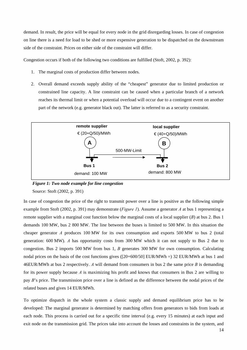
Figure 1: Two node example for line congestion

Source: Stoft (2002, p. 391)

In case of congestion the price of the right to transmit power over a line is positive as the following simple

example from Stoft (2002, p. 391) may demonstrate (Figure 1). Assume a generator A at bus 1 representing a

remote supplier with a marginal cost function below the marginal costs of a local supplier (B) at bus 2. Bus 1

demands 100 MW, bus 2 800 MW. The line between the buses is limited to 500 MW. In this situation the

cheaper generator A produces 100 MW for its own consumption and exports 500 MW to bus 2 (total

generation: 600 MW). A has opportunity costs from 300 MW which it can not supply to Bus 2 due to

congestion. Bus 2 imports 500 MW from bus 1, B generates 300 MW for own consumption. Calculating

nodal prices on the basis of the cost functions gives ([20+600/50] EUR/MWh =) 32 EUR/MWh at bus 1 and

46EUR/MWh at bus 2 respectively. A will demand from consumers in bus 2 the same price B is demanding

for its power supply because A is maximizing his profit and knows that consumers in Bus 2 are willing to

pay B’s price. The transmission price over a line is defined as the difference between the nodal prices of the

related buses and gives 14 EUR/MWh.

To optimize dispatch in the whole system a classic supply and demand equilibrium price has to be

developed: The marginal generator is determined by matching offers from generators to bids from loads at

each node. This process is carried out for a specific time interval (e.g. every 15 minutes) at each input and

exit node on the transmission grid. The prices take into account the losses and constraints in the system, and

15

generators are dispatched by the system operator, not only in ascending order of offers (or descending order

of bids), but in accordance with the required security of the system. This results in a spot market with bid-

based, security-constrained, economic dispatch with nodal prices as proposed by Hogan (2003, p. 2).

Apparently, nodal prices reflect the actual situation in the grid more transparently than uniform prices and

represent adequate allocation signals. The calculation nodal prices is one of several important considerations

in analyzing where to site additional generation, transmission and load. The implementation of efficient

congestion management methods on the basis of nodal pricing is crucial to cope with scarce transmission

capacities and to ensure security of supply. In combination with further political measures there might be

saved costly investments in transmission lines (see Bower, 2004).

Nodal pricing was first implemented in New Zealand (1997), followed by some US markets (e.g. PJM 1998,

New York 1998, New England 2003).7 On 1 April 2005, the British Electricity Trading and Transmission

Arrangements (“BETTA”) were introduced in UK extending the earlier “New Electricity Trading

Arrangements” for England and Wales (NETA) to Scotland. With BETTA, nodal pricing was introduced for

the Great Britain grid on the basis of marginal transmission investment requirements (Tornquist, 2005). The

California ISO is actually redesigning the procedures by which it performs forward scheduling and

congestion management; CAISO plans to introduce nodal pricing by 2007 CAISO (2005).

2.2.4 Empirical studies on nodal pricing

Empirical analyses using the nodal pricing concept have been provided, e.g. for England/Wales, Austria,

Italy and, most recently, for California. A contentious issue is how to model the electrical grid properly and,

thereupon, how to calculate corresponding nodal prices. On the basis of data from the U.S. Midwest region

the full AC model was compared to the less complex DC Load Flow model.

Green (2004) developed a thirteen node model of the transmission system in England and Wales

incorporating losses and transmission constraints. The study analyzes the impact of different transmission

pricing schemes (LMP, zonal and uniform pricing). Green shows that the introduction of the LMP concept

would raise welfare by 1.5% compared to the uniform model on behalf of the larger consumer welfare

(+2.6%) while generator profit would decrease by 1.1%. To strengthen these results, Green applies different

values for demand elasticity (-0.1, -0.25, -0.4) and shows that the increase of welfare is higher with a larger

absolute elasticity value.

For the Austrian high voltage grid, Todem (2005) has analyzed the economic impact of a nodal price based

congestion management. Against the background of scarce transmission capacities in the East of Austria,

7 According to Fuller (2005), nodal pricing was introduced even earlier in some Latin American states (Chile 1982, Argentina 1992, Peru 1993, Bolivia 1994).

16

Todem developed an optimization model with 165 nodes applicable to the bilateral Austrian electricity

market.8 On the basis of January 2004 data, it could be shown, in which places congestion occurs and which

prices would be optimal. The author suggests a division of the network into two pricing zones according to

their congestion situation. The most efficient solution to overcome the congestion problem would be to build

an additional 380-kV line – the so called ‘Steiermark’-line.

Interesting results regarding the distribution of economic surplus under nodal, uniform and zonal pricing

provides a study from Ding and Fuller (2005). They show for the Italian 400 kV grid that there is no loss in

(total) social surplus using uniform or zonal pricing with a nodal pricing dispatch compared to a full nodal

price system (dispatch and pricing nodal-based). The authors therefore calculated optimal dispatch on the

basis of an optimal power-flow model, respecting transmission constraints and losses while defining uniform

(respectively zonal) prices for financial settlements. The results, however, show that the distribution of

economic surplus between supply and demand sides will vary depending on the pricing model. More

importantly, the authors reveal perverse incentives for generators that are dispatched at different levels than

uniform or zonal prices would suggest. “Constrained-on” generators, which are dispatched at higher levels,

may receive a smaller surplus than under nodal pricing settlement, even though the extra generation is

needed (and vice versa for “constrained-off” generators). However, as economic data of the study where not

completely realistic, the authors did not draw firm conclusions.

The California ISO has – in the run-up to the planned implementation of its Market Redesign and technology

Upgrade (MRTU)9- provided several studies on locational marginal pricing. The most recent one (August

2005) uses schedules and market bids of previous years, conditions of the future MRTU structure and the

ISO’s full network model in an Alternating Current (AC) Optimal Power Flow (OPF) simulation to estimate

prices that may occur in the ISO’s real-time market if it were based on locational marginal prices (CAISO

2005, p. 1). Prices were calculated and given as average per zone (total of 29 zones). The resulting LMPs are

generally moderate, apart from some exceptions: less 1% of the nodal prices exceeded $100/MWh, and 91%

of the nodal prices were below $65. Furthermore, prices within one zone were generally very similar while

significant zonal price variations last only a few hours per year. In conclusion, it was found that LMP pricing

would produce stable and predictable prices. This result may refute concerns regarding the potential for high

LMPs in certain constrained areas of the grid, where the cost of delivering energy to customers is increased

due to frequent, severe congestion.

8 Other electricity markets using the nodal price approach are usually centrally organized (PJM Interconnection, NYISO and New

Zealand). 9 The MRTU proposes a forward and real-time congestion management procedure that adjusts generation, load, import, and export

schedules to clear congestion using an Alternating Current (AC) Optimal Power Flow algorithm (OPF) and a Full Network Model (FNM) that includes all buses and transmission constraints within the CAISO Control Area. (CAISO, 2005, p. 4)

17

2.3 Technical specifics

2.3.1 Transmission capacity constraints

The transmission of energy by electricity follows specific physical laws. Every current flow in a transmission

line rises the temperature of the line. Each line has a maximum temperature it can sustain (thermal limit).

The change in temperature is proportional to the resistance of a transmission line. An easy example for the

relationship of a line resistance is given by:

* lRA

ρ= (2.1)

The circuit resistance depends on its cross section (and the resulting surface area), the length of the line, and

the used material. Moreover, the transmission capacity depends on several factors such as the number of

circuits, the environmental temperature and wind conditions. Accordingly, the transmission limit is not a

constant value but changes along with external factors. Hence, equation (2.1) is accurate for illustrative

reasons but not applicable in real transmission systems. Under real conditions, empirically acquired data for

resistances and reactances are used that already include the above mentioned characteristics.10

Altogether, physical facts implicate that the maximum energy flow is limited. In case the thermal limit is

passed, undisturbed operation is not longer guaranteed and therefore requires a regulation of flows. If the

overstepping is high in magnitude or lasts for a longer period, respectively, transmission lines may tear apart

due to decreasing mechanical strength. This situation is referred to as congestion on line.

As explained above, a current flow causes a change in temperature. Unfortunately this comes along with an

energy loss in this transmission line:

- Ohm’s law: V=R*I (2.2)

- Power law: P=V*I (2.3)

Inserting equation (2.2) in (2.3) yields:

- Loss of a DC transmission line: P=R*I2 (2.4)

An AC model fully considers the line impedance Z consisting of resistance (real part) and reactance (reactive

part). Section 3.2 describes how the DC Load Flow model simplifies the problem.

10 See section 3.4 for the approximate values that are used in this report.

18

2.3.2 Kirchoff’s laws

2.3.2.1 Kirchhoff’s first law (current law)

The electrical DC current is equal to the number of charge carriers flowing through a line within a specific

time or, in case of AC, the frequency with which the charge carrier pulsate. Kirchhoff’s first law – also

called: current law – specifies that these charge carriers cannot disappear. The sum of incoming flows must

equal the sum of outgoing flows. Defining the incoming current as positive and the outgoing as negative, the

sum will be zero:

0µµ

I =∑ (2.6)

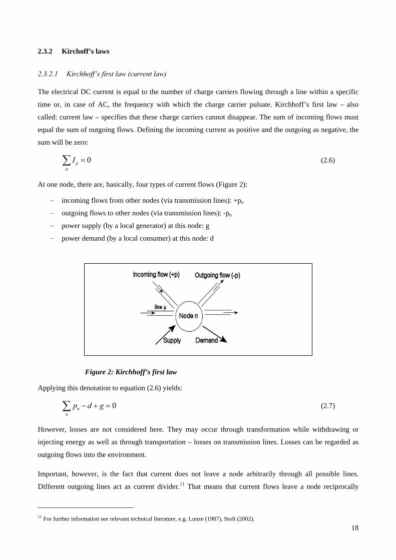
At one node, there are, basically, four types of current flows (Figure 2):

- incoming flows from other nodes (via transmission lines): +pn

- outgoing flows to other nodes (via transmission lines): -pn

- power supply (by a local generator) at this node: g

- power demand (by a local consumer) at this node: d

Figure 2: Kirchhoff’s first law

Applying this denotation to equation (2.6) yields:

0nn

p d g− + =∑ (2.7)

However, losses are not considered here. They may occur through transformation while withdrawing or

injecting energy as well as through transportation – losses on transmission lines. Losses can be regarded as

outgoing flows into the environment.

Important, however, is the fact that current does not leave a node arbitrarily through all possible lines.

Different outgoing lines act as current divider.11 That means that current flows leave a node reciprocally

11 For further information see relevant technical literature, e.g. Lunze (1987), Stoft (2002).

19

proportional to the resistances of the respective lines. The effect is that one cannot inject more energy at this

node once on of the outgoing lines is congested even if other lines are still able to work with higher load.

This is, particularly, decisive in highly meshed networks. For those meshed networks, the second Kirchhoff

law has to be considered as well.

2.3.2.2 Kirchhoff’s second law (voltage law)

Voltage describes the difference between two electric potentials. You could say voltage makes current

flow.12 Power plants create and sustain a potential difference throughout the grid. If energy was consumed

without energy injection into the grid voltage would collapse. Hence, consumption can be understood as

voltage drain. The second law of Kirchhoff states that the sum of all voltages within a mesh equals zero –

equation (2.8).

0Vνν

=∑ (2.8)

The above explained technical specifics are not primarily of economic relevance. However, they make up the

framework for an economic consideration of electricity networks. For deeper matter compare Koettnitz and

Pundt (1967), Koettnitz et al (1986), Lunze (1987).and Stoft (2002).

3 Model and Data

3.1 Optimization problem

A standard DC load flow model was used to simulate the German high voltage transmission system. The grid

comprises 291 nodes (plus 19 auxilliary nodes, see section 3.4.1) and two voltage levels (380 and 220 kV).

For more detailed information about the DC Load Flow model and underlying assumptions see section 3.2.

This report follows the path described by Schweppe et al (1988). His work provides the mathematical basis

for our model. According to the programming example outlined by Todem (2004, pp. 85-101) and with

valuable personal help of Mr Todem himself, the modelling software GAMS13 is utilized to implement the

necessary mathematical equations.

In case of a convex problem, GAMS solves a set of equations by means of iteration processing. GAMS

therefore offers a set of solvers varying in the way of finding a solution. Generally spoken, the type of

12 For further information see relevant technical literature, e.g. Lunze (1987), Stoft (2002). 13 GAMS optimizes an objective function and fulfils additional side conditions simultaneously.

20

problem, e.g. linear or nonlinear, determines the range of possible solvers. In our experience the solvers

Pathnlp and Conopt are appropriate for this model which is non linear. Both lead to the same results.

In this study, a static approach was chosen. Different scenarios were computed separately, analysed, and,

subsequently, compared to each other. The period of time referred to is one hour. For reasons of simplicity,

we do not consider a transmission reliability margin [(N-1)-constraint]. The model stresses transmission lines

up to 100% of their thermal limit. This must be taken into account while analyzing results.

3.1.1 Cost minimization under uniform pricing

In both the nodal and the uniform pricing model social welfare is the objective value to maximize. The

welfare equals total consumers’ benefit minus costs of generation, what is identical to the sum of producers’

and consumers’ surplus (Figure 3).14 The model determines optimal dispatch quantities of generation and

loads as well as the voltage angles at each bus while respecting the physical laws of power flow, particularly

Kirchhoff’s laws, capacity constraints of lines and generators, and demand characteristics. In the case of a

uniform price, the price and demand per node are fixed. This is an admissible simplification for the static

approach. In order to maximize welfare, the cost minimal dispatch has to be found. Hence, it becomes a cost

minimization problem.

∑ ∫∫⎟⎟⎟

⎠

⎞

⎜⎜⎜

⎝

⎛⋅−⋅=

n

drefn

refn

refn

drefnref

refn

refn

refn

dddcdddpdW00

)()()(max (1)

s.t. maxii PP ≤ line flow constraint (2)

∑∑ +=n

nn

n Ldg energy balance constraint (3)

∑∑ ≤tn

tn

tn

tn gg

,

max,

, generation constraint (per type of plant) (4) 15

Total costs comprise only marginal costs of production at the power plants. Other costs as e.g. those arising

from network operation and maintenance are neglected.

3.1.2 Nodal pricing

In the case of nodal prices, welfare is maximized by finding the optimal demand for each node (Figure 3).

Hence, the following set of equations has to be solved.16

14 Aee Appendix A. 15 For a detailed description of all equations and constraints as used in the GAMS code see Appendix Appendix B. 16 Constraints to be obtained are the same as above. Compare also: Hsu (1997) and Green (2004).

21

∑ ∫∫ ⎟⎟

⎠

⎞

⎜⎜

⎝

⎛⋅−⋅=

n

d

nnn

d

nnnn

dddcdddpdW**

0

***

0

*** )()()(max (5)

s.t. maxii PP ≤ line flow constraint (6)

∑∑ +=n

nn

n Ldg energy balance constraint (7)

∑∑ ≤tn

tn

tn

tn gg

,

max,

, generation constraint (per type of plant) (8)

Figure 3: Social welfare and market clearing price

Having the optimal dispatch for every node dn*, the corresponding market clearing nodal price pn is given by

the inverse demand function:17

⎟⎟⎠

⎞⎜⎜⎝

⎛−⋅⋅+= 11 *

refn

nrefn

refnn d

dppp

ε (9)

17 Derivation of this equation is presented in Appendix A.

price

supply, demand (quantity of power)

pnref

pn

dnref

merit order

(supply)

costs of production

social welfare

inverse demand

function

dn*

consumer surplus

producer surplus

22

3.2 The DC Load Flow Model

3.2.1 Why DC

In general, Schweppe et al (1988) showed that the DC Load Flow Model (DCLF) can be used as an

instrument for an economic analysis of electricity networks. They apply it to their nodal price approach for

electricity pricing. As calculations in electricity networks are sophisticated due to the occurrence of reactive

power and the flow characteristic of electricity in highly meshed HV networks, simplifications are necessary.

The DCLF helps to simplify the modeling of such networks in case of symmetrical steady states. The DCLF

focuses on real power flows. It is, in particular, applicable for economic purposes as the transport of real

power is the main task of electricity networks (Todem et al, 2005, p. 5). Hence, real power is the main

commodity that customers demand and that generates benefits.18

Overbye et al (2004, p. 2) emphasize three advantages of the DCLF compared to an AC model:

1. The problem becomes smaller (about half the size).

2. The solution is noniterative.

3. The network topology does not depend on the power flowing and has to be factored once only.

Furthermore, they come to the conclusion that the DCLF is adequate for modeling LMPs albeit there are

some buses at which the deviation is significantly high. The latter occurs particularly on lines with high

reactive power and low real power flows (Overbye et al, 2004, p. 4). This is easily understandable because as

above mentioned reactive power is ignored by the DC approach.

3.2.2 The model

3.2.2.1 Foundations

Schweppe et al (1988, pp. 272-274) describe the way from a complete AC Load Flow to a DCLF. Therefore,

a decoupled AC Load Flow model is generated which assumes that real power P flows according to the

differences of the voltage angles Θjk between two nodes as well as reactive power flows Q is caused by

differences in voltage magnitudes V. Consequently, one can model the real power flow by only focusing on

voltage angle differences. The paper of Stigler and Todem (2005, pp. 114-115) explains the basic equations

that are described by Schweppe et al in detail:

jkkjijkkjijijk Θ · VV B Θ · VV - GVG P sincos2

+= (3.10)

18 Relevant reactive power issues such as the necessity or influence, respectively, of investments in compensation facilities can not be modeled by DC flows.

23

( )kj δδ −=Θ jk (3.11)

22ii

ii

RX

XB

+= (3.12)

22ii

ii

RX

RG

+= (3.13)

Equation (3.10) is the basis for all further calculations – both the lossless DC load flow and the transmission

losses (Stigler and Todem, 2005, pp. 116-118). Moreover, two basic assumptions must be made (Schweppe,

1988, p. 314):

1. The voltage angle difference Θjk is very small.

2. The voltage magnitudes V are standardized to per unit calculation. Hence, they can be considered to

be equally one at each node (Vj ≈ Vk).

3.2.2.2 Real power flow between two nodes

The calculation of lossless real power flows is the first step along the way to use the DCLF in a dynamic

economic model of an electricity network. In order to approximate the lossless line flows, one can suppose

that:

1 cos jk ≈Θ (3.14)

jkjk Θ≈Θsin (3.15)

This yields a linear equation for the lossless line flows:

jkijk BP Θ⋅= (3.16)

3.2.2.3 Losses of real power between two nodes

The second step along the way is the estimation of losses occurring along the lines. Losses are important as

they cause the sum of generation not to equal the sum of demand. Thus, transmission lines are stressed not

only by demand but by demand plus losses. In order to approximate the losses on a line, equation (3.14)

must be complemented by the second order term of the Taylor series approximation:

2-1 cos

2

jkjkΘ

≈Θ (3.17)

24

Then, after some further assumptions and conversions19 transmission losses can be calculated by:

2jkijk PRL ⋅= (3.18)

Both equations (3.16) and (3.18) provide us with the required relationship between demand and generation

as well as the resulting real power flow. One can now start to implement the model in order to observe

changes in line flows caused by changes in demand or generation, respectively. Combining this with a set of

economic information such as demand and supply functions for each node will enable us to assign a specific

price for each node of the network.

3.3 Description of the GAMS modeling process

For a better understanding of the GAMS code the modeling process will be described exemplarily for the

nodal price approach following the code which is divided into 5 parts.20

During the optimization process GAMS changes demand in the system in conformity with a given demand

function21, which defines the price the consumer is willing to pay at most. This is done by means of varying

the voltage angles at each node. Following the merit order of generation and given the reference price,

GAMS herewith calculates the maximum welfare at each node and – after aggregation - for the whole

system.

Part I

First of all, each node is assigned a number from 1 to 310. Similarly, each line is given a number from 1 to

407. For subsequent standardization fixed base values are defined for apparent power and the two voltage

levels. Additionally, fixed demand elasticity for all demand functions is introduced.

Part II

Here, data in from of fixed parameters representing the real situation in Germany is included into the GAMS

code. Parameters are:

• reference points per node (prices and demands),

• thermal limits of each line,

• generation capacities per node and costs per plant type.

19 See Appendix C. 20 The uniform pricing model is calculated respectively merely modifying the objective function as described in section 3.1.2. 21 See section 3.4.5 and Appendix A for more detailed information about the underlying demand function.

25

The thermal line limit is calculated according to Lunze (1987, p. 222)22:

maxmax 3 IVP = (3.19)

In (3.19) V is the given voltage level of the line. I represents the given maximum current at a line without

overheating and damaging the line.

The mix of generation plant types defines the maximum supply capacity per node. Except wind stations,

different marginal costs of production are defined for each type. Wind mills do not have variable costs and

therefore no marginal costs. However, they increase the need for balancing and response capacity within the

network because the intensity and duration of wind is difficult to predict. These costs are estimated and taken

into account as opportunity costs.

Part III

The transfer matrix H and the network susceptance matrix B are computed. They contain all necessary

information about the network topology and the normalized reactances and resistances of the lines. H is the

product of the line susceptance vector (B-Vector, see Appendix Appendix B, p. 51) and the incidence

matrix. B is the sum of the products of the incidence matrix and the transfer matrix H over all lines. Node 1

is appointed to be the swing bus of the network.

Part IV

Power input per node is calculated as the sum of nine sub variables representing the nine different plant types

that are, generally, able to contribute to the nodes power generation. In order to calculate the total variable

costs of generation per node the amount of power generated by a plant is multiplied by its marginal costs of

production. Consequently, this sum is a variable, too.

The net input is calculated as the difference between input and demand plus losses. In case of a net input

unequal zero, there is a voltage angle between the node’s voltage vector and the voltage vector at the swing

bus, which results in a flow of power.

Part V

Respecting all necessary constraints, the welfare function as described above is maximized. The resulting

optimal quantity of power demanded at every node dn* is used to calculate nodal prices pn on the basis of the

inverse demand equation as given in (A.8). This is the price a consumer at node n is at most willing to pay

for the calculated quantity of power.

22 Note that in a DC world apparent power (S) equals real power (P).

26

3.4 Data

The subsequent section describes the empirical data used in the model. First of all, a survey of the required

input variables is given; afterwards the calculations and the underlying approaches are explained.

3.4.1 Mapping the high voltage-network

The nodes are taken as the substations from the German integrated network (VGE, 2000, UCTE, 2004). Only

substations of the high and extra high voltage level were taken into consideration under the assumption that

the entire electricity transportation for all voltage levels takes place through high voltage transmission.

Hence, 291 regular plus 19 auxiliary nodes within the 380 kV and the 220 kV levels were detected (Table 2).

Auxiliary nodes became necessary where lines split up without a node or where the course of a line is

ambiguous (Figure 4).

Figure 4: Example for an auxiliary node Source: UCTE (2004).

Lines of different voltage levels are listed separately, so the there may be more than one connection between

two nodes, e.g. one 380 kV double circuit and one 220 kV double circuit. Our model embraces 426

electricity lines for Germany. It does not include cross-border flows.

27

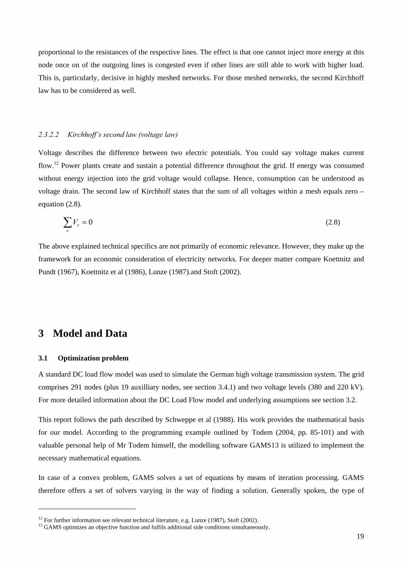
Table 2: Details of the high voltage-network

3.4.2 Line specific data

A line’s characteristic can be described by three main factors: maximum thermal limit, line resistance and

line reactance. The maximum thermal limit is, basically, influenced by the type and the length of the line as

well as by the voltage level (see section 2.3.1). For Germany, we assumed four cables23 per wire for 380 kV

circuits and two cables24 per wire for the 220kV level (Pundt, 1983, p. 11 et seq., Pundt and Schegner, 1997,

p. 38 et seq.). An adequate value for the apparent power S is 1500 MVA for the 380 kV level up to a length

of 100 km, and, respectively, 400 MVA for a 220 kV level circuit up to a length of 90 km (Pundt, 1983,

p. 11). In fact, the admissible apparent power decreases for a continuous line longer than the given lengths

(ibid.).

From equation (3.19) maximal current can be derived as follows:

V

SI*3max = (3.20)

In our model the possible current doubles when using a double circuit line, and is three times larger for a

triple circuit line. These maximal current values are necessary for the maximum power flow constraint in the

model.

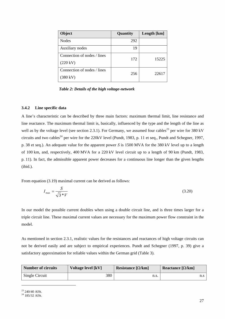
As mentioned in section 2.3.1, realistic values for the resistances and reactances of high voltage circuits can

not be derived easily and are subject to empirical experiences. Pundt and Schegner (1997, p. 39) give a

satisfactory approximation for reliable values within the German grid (Table 3).

Number of circuits Voltage level [kV] Resistance [Ω/km] Reactance [Ω/km]

Single Circuit 380 n.s. n.s

23 240/40 AlSt. 24 185/32 AlSt.

Object Quantity Length [km]

Nodes 292

Auxiliary nodes 19

Connection of nodes / lines

(220 kV) 172 15225

Connection of nodes / lines

(380 kV) 256 22617

28

220 n.s n.s

Double circuit 380 0.03 0.26

220 0.078 0.29

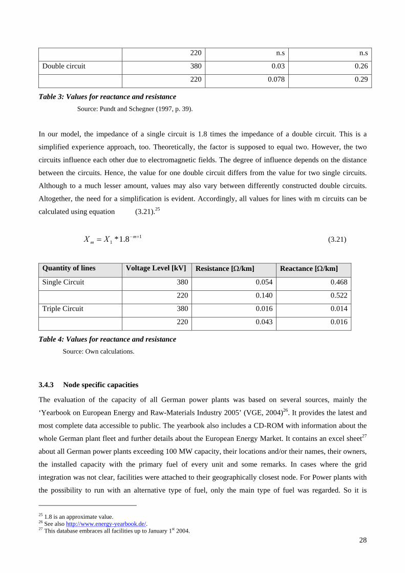
Table 3: Values for reactance and resistance Source: Pundt and Schegner (1997, p. 39).

In our model, the impedance of a single circuit is 1.8 times the impedance of a double circuit. This is a

simplified experience approach, too. Theoretically, the factor is supposed to equal two. However, the two

circuits influence each other due to electromagnetic fields. The degree of influence depends on the distance

between the circuits. Hence, the value for one double circuit differs from the value for two single circuits.

Although to a much lesser amount, values may also vary between differently constructed double circuits.

Altogether, the need for a simplification is evident. Accordingly, all values for lines with m circuits can be

calculated using equation (3.21).25

1

1 8.1* +−= mm XX (3.21)

Quantity of lines Voltage Level [kV] Resistance [Ω/km] Reactance [Ω/km]

Single Circuit 380 0.054 0.468

220 0.140 0.522

Triple Circuit 380 0.016 0.014

220 0.043 0.016

Table 4: Values for reactance and resistance Source: Own calculations.

3.4.3 Node specific capacities

The evaluation of the capacity of all German power plants was based on several sources, mainly the

‘Yearbook on European Energy and Raw-Materials Industry 2005’ (VGE, 2004)26. It provides the latest and

most complete data accessible to public. The yearbook also includes a CD-ROM with information about the

whole German plant fleet and further details about the European Energy Market. It contains an excel sheet27

about all German power plants exceeding 100 MW capacity, their locations and/or their names, their owners,

the installed capacity with the primary fuel of every unit and some remarks. In cases where the grid

integration was not clear, facilities were attached to their geographically closest node. For Power plants with

the possibility to run with an alternative type of fuel, only the main type of fuel was regarded. So it is

25 1.8 is an approximate value. 26 See also http://www.energy-yearbook.de/. 27 This database embraces all facilities up to January 1st 2004.

29

feasible to cover the demand with the most convenient power plants, because it is required that the main fuel

is the most advantageous fuel for every plant.28

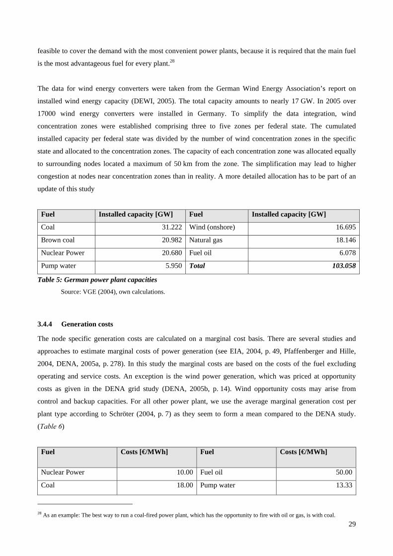
The data for wind energy converters were taken from the German Wind Energy Association’s report on

installed wind energy capacity (DEWI, 2005). The total capacity amounts to nearly 17 GW. In 2005 over

17000 wind energy converters were installed in Germany. To simplify the data integration, wind

concentration zones were established comprising three to five zones per federal state. The cumulated

installed capacity per federal state was divided by the number of wind concentration zones in the specific

state and allocated to the concentration zones. The capacity of each concentration zone was allocated equally

to surrounding nodes located a maximum of 50 km from the zone. The simplification may lead to higher

congestion at nodes near concentration zones than in reality. A more detailed allocation has to be part of an

update of this study

Fuel Installed capacity [GW] Fuel Installed capacity [GW]

Coal 31.222 Wind (onshore) 16.695

Brown coal 20.982 Natural gas 18.146

Nuclear Power 20.680 Fuel oil 6.078

Pump water 5.950 Total 103.058

Table 5: German power plant capacities Source: VGE (2004), own calculations.

3.4.4 Generation costs

The node specific generation costs are calculated on a marginal cost basis. There are several studies and

approaches to estimate marginal costs of power generation (see EIA, 2004, p. 49, Pfaffenberger and Hille,

2004, DENA, 2005a, p. 278). In this study the marginal costs are based on the costs of the fuel excluding

operating and service costs. An exception is the wind power generation, which was priced at opportunity

costs as given in the DENA grid study (DENA, 2005b, p. 14). Wind opportunity costs may arise from

control and backup capacities. For all other power plant, we use the average marginal generation cost per

plant type according to Schröter (2004, p. 7) as they seem to form a mean compared to the DENA study.

(Table 6)

Fuel Costs [€/MWh] Fuel Costs [€/MWh]

Nuclear Power 10.00 Fuel oil 50.00

Coal 18.00 Pump water 13.33

28 As an example: The best way to run a coal-fired power plant, which has the opportunity to fire with oil or gas, is with coal.

30

Brown coal 15.00 Running wasser 0.00

Natural Gas 40.00 Wind 4.05

Table 6: Marginal costs of power generation per fuel Source: DENA (2005b) and Schröter (2004).

3.4.5 Demand

In order to derive node-specific demand, we assume a positive correlation between economic income and

total electricity demand. We split the federal states into administrative local districts and identified their

population figures (DESTATIS, 2005). Inhabitants per node were calculated distributing a district’s

population figure equally to all nodes of the district. In a second step, annual per capita energy consumption

had to be determined for every node. Therefore, the annual average per capita energy consumption of

Germany as given by German Federal Statistical Office (DESTATIS, 2005) was multiplied by the ratios of

Germany’s total GDP and the federal states specific GDP (Statistik-Portal, 2005). This resulted in a weighted

per capita consumption for every federal state. All nodes within one federal state were assumed to have the

same per capita consumption. Multiplying the annual per capita consumption of a node by its population

figure and dividing this by 8,760 finally gives the hourly node specific demand. Summing up the nodes’

demand resulted in a total demand of 56,241 MWh.

A disadvantage of the received data is that the results are average values. This lowers the signification of the

model because the variability of demand remains unconsidered. In order to solve this problem, the node

specific demands will be modified in different scenarios and adjusted by system load data of the respective

transmission system operators.

Federal state Ratio

GDPF/GDPG

Number of local

districts

Hourly demand per

federal state [MWh]

Baden-Wurttemberg 1.10 44 8,287

Bavaria 1.11 96 9,720

Berlin 0.85 1 2,053

Brandenburg 0.66 18 1,198

Bremen 1.32 2 0,669

Hamburg 1.66 1 2,065

Hesse 1.19 26 5,100

Mecklenburg-Western Pomerania 0.64 18 0,784

Lower Saxony 0.86 46 5,006

North Rhine-Westphalia 0.96 54 12,294

Rhineland-Palatinate 0.85 36 2,400

31

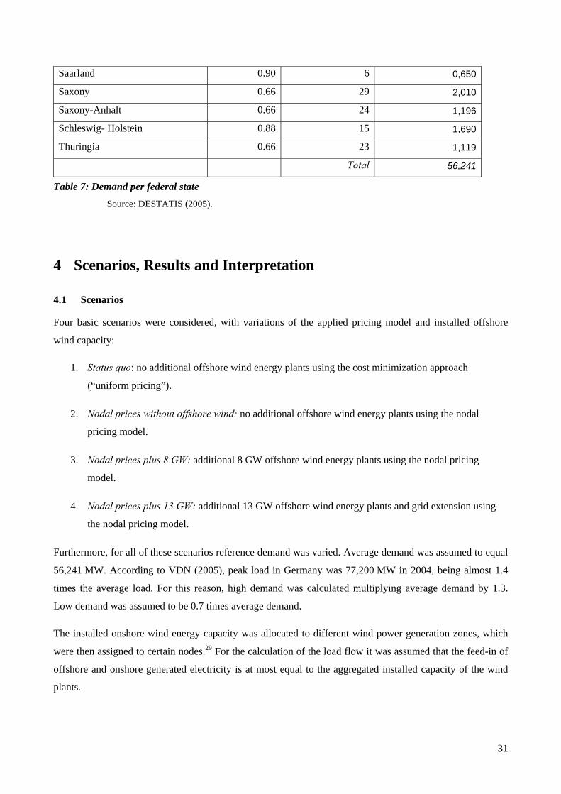
Saarland 0.90 6 0,650

Saxony 0.66 29 2,010

Saxony-Anhalt 0.66 24 1,196

Schleswig- Holstein 0.88 15 1,690

Thuringia 0.66 23 1,119

Total 56,241

Table 7: Demand per federal state Source: DESTATIS (2005).

4 Scenarios, Results and Interpretation

4.1 Scenarios

Four basic scenarios were considered, with variations of the applied pricing model and installed offshore

wind capacity:

1. Status quo: no additional offshore wind energy plants using the cost minimization approach

(“uniform pricing”).

2. Nodal prices without offshore wind: no additional offshore wind energy plants using the nodal

pricing model.

3. Nodal prices plus 8 GW: additional 8 GW offshore wind energy plants using the nodal pricing

model.

4. Nodal prices plus 13 GW: additional 13 GW offshore wind energy plants and grid extension using

the nodal pricing model.

Furthermore, for all of these scenarios reference demand was varied. Average demand was assumed to equal

56,241 MW. According to VDN (2005), peak load in Germany was 77,200 MW in 2004, being almost 1.4

times the average load. For this reason, high demand was calculated multiplying average demand by 1.3.

Low demand was assumed to be 0.7 times average demand.

The installed onshore wind energy capacity was allocated to different wind power generation zones, which

were then assigned to certain nodes.29 For the calculation of the load flow it was assumed that the feed-in of

offshore and onshore generated electricity is at most equal to the aggregated installed capacity of the wind

plants.

32

It was first checked whether nodal pricing was superior to cost minimization under uniform pricing regarding

the respective social welfares (section 4.2.1). To ensure comparability of these scenarios, the same input data

were used. Within the nodal price scenario demand and price could vary, whereas, the cost minimization

approach works with a given uniform price. Neither of these scenarios considers the integration of additional

offshore wind energy. Thus, the impact on social welfare of introducing a competitive nodal pricing scheme

in Germany compared to the current situation is obtained.

In a next step additional offshore wind energy plants were integrated into the existing grid (section Fehler!

Verweisquelle konnte nicht gefunden werden.). The aim was to find out how much offshore wind energy

could be fed into the grid at most without any extension of lines. Consequently, they were not considered in

the model, which is based on marginal costs. Offshore wind energy from the North Sea was supposed to be

fed in completely at nodes along the coastline (Brunsbüttel, Emden, Wilhelmshaven). Having calculated

occurring congestions, GAMS would reduce input of offshore energy if congestion costs exceeded

opportunity costs of wind energy. Therewith, this scenario shows the maximum possible offshore feed in

considering the existing grid.

Finally, a scenario was run considering additional 13 GW offshore wind energy plant (section 4.2.3).30 In our

model, this would require an extension of the grid by four lines and an upgrade of two lines.31 Fix costs from

an expansion of plant and grid capacity were neglected and offshore energy supposed to be fed into nodes at

the coast.

Scenario Demand at

loads

Price Capacity of offshore

wind energy plants

Grid capacity

1. Status quo

low

average

high

fix 0 GW existing lines

2. Nodal prices without

offshore wind

low

average

high

nodal 0 GW existing lines

3. Nodal prices plus 8 GW

low

average

high

nodal 8 GW existing lines

(full capacity)

4. Nodal prices plus 13 GW

low

average

high

nodal 13 GW grid extension

29 In this study no geographical differences in the strength of wind (e.g. strong wind vs. light wind) were adopted. In case of distinguishing wind generated electricity by regions, a higher load on the transmission lines from North to South and from East to West would result (DENA, 2005a, p. 75 et sqq.). 30 The DENA grid study (DENA, 2005a) proposes offshore wind capacities of 20 GW until 2020. 31 These lines are planned to construct according to VGE (2000).

33

Table 8: Scenarios

In the subsequent chapter results will be discussed. Scenarios will be compared as following:

• Status quo vs. nodal prices without offshore wind (scenario 1 vs. scenario 2)

• Nodal prices without wind vs. nodal prices plus 8 GW (scenario 2 vs. scenario 3)

• Nodal prices plus 8 GW vs. nodal prices plus 13 GW (scenario 3 vs. scenario 4)

4.2 Results and Interpretation

4.2.1 Existing HV-grid: scenario 1 vs. scenario 2

First we compared nodal pricing with the cost minimization under uniform pricing. The results refer to

hourly values. Marginal cost bidding and a demand elasticity of -0.25 at the reference point are supposed. In

order to define the reference price, the EEX average price32 for the relevant period – same as for demand

calculation – was estimated using the 200-day-line.

32 Note that the EEX volumes at the moment only account for approximately 10% of the entire market volume.

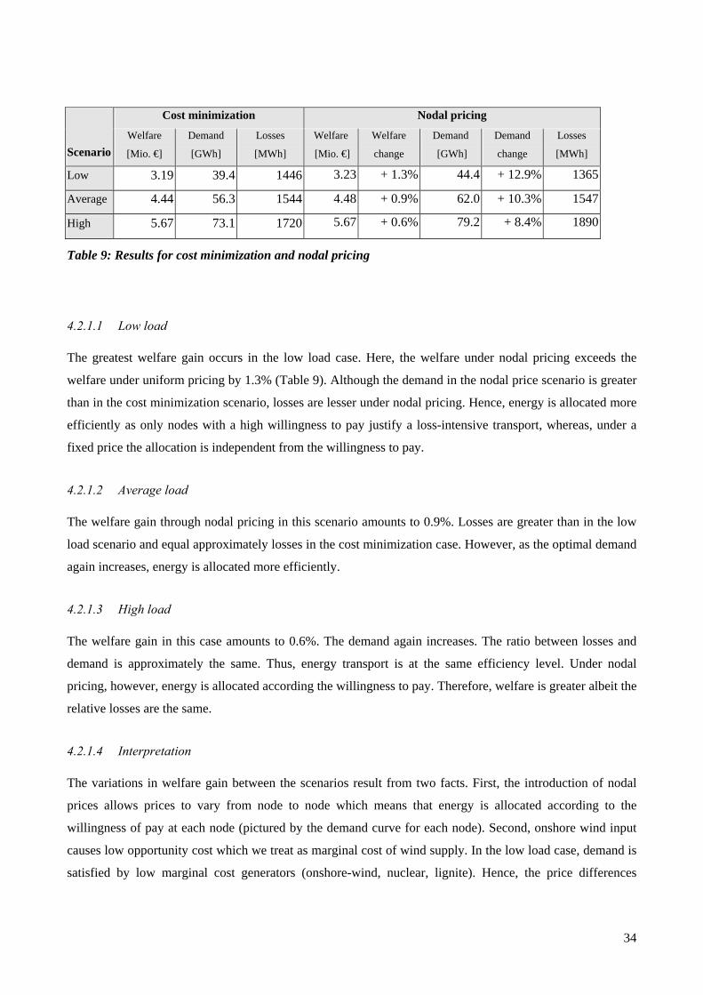
34

Table 9: Results for cost minimization and nodal pricing

4.2.1.1 Low load

The greatest welfare gain occurs in the low load case. Here, the welfare under nodal pricing exceeds the

welfare under uniform pricing by 1.3% (Table 9). Although the demand in the nodal price scenario is greater

than in the cost minimization scenario, losses are lesser under nodal pricing. Hence, energy is allocated more

efficiently as only nodes with a high willingness to pay justify a loss-intensive transport, whereas, under a

fixed price the allocation is independent from the willingness to pay.

4.2.1.2 Average load

The welfare gain through nodal pricing in this scenario amounts to 0.9%. Losses are greater than in the low

load scenario and equal approximately losses in the cost minimization case. However, as the optimal demand

again increases, energy is allocated more efficiently.

4.2.1.3 High load

The welfare gain in this case amounts to 0.6%. The demand again increases. The ratio between losses and

demand is approximately the same. Thus, energy transport is at the same efficiency level. Under nodal

pricing, however, energy is allocated according the willingness to pay. Therefore, welfare is greater albeit the

relative losses are the same.

4.2.1.4 Interpretation

The variations in welfare gain between the scenarios result from two facts. First, the introduction of nodal

prices allows prices to vary from node to node which means that energy is allocated according to the

willingness of pay at each node (pictured by the demand curve for each node). Second, onshore wind input

causes low opportunity cost which we treat as marginal cost of wind supply. In the low load case, demand is

satisfied by low marginal cost generators (onshore-wind, nuclear, lignite). Hence, the price differences

Cost minimization Nodal pricing

Scenario Welfare

[Mio. €]

Demand

[GWh]

Losses

[MWh]

Welfare

[Mio. €]

Welfare

change

Demand

[GWh]

Demand

change

Losses

[MWh]

Low 3.19 39.4 1446 3.23 + 1.3% 44.4 + 12.9% 1365

Average 4.44 56.3 1544 4.48 + 0.9% 62.0 + 10.3% 1547

High 5.67 73.1 1720 5.67 + 0.6% 79.2 + 8.4% 1890

35

between nodal prices and the uniform price is greatest.33 Combining this with the two facts mentioned above,

it can be shown that the welfare spread between uniform and nodal pricing is largest during low load periods

as the uniform price error is largest. Onshore wind generators, however, are predominantly located in

Northern and Central Germany but inject energy into many different nodes and can, thus, be sufficiently

transmitted throughout the country. Remarkably, the same lines are congested comparing uniform and nodal

pricing scenario. Taking congestions into account and thus pricing energy efficiently leads to higher demand

and lower – but differing – prices (Figure 5).

0,00

5,00

10,00

15,00

20,00

25,00

30,00

35,00

1 17 33 49 65 81 97 113 129 145 161 177 193 209 225 241 257 273 289 305

node

€/M

Wh

nodal price uniform price

Figure 5: Nodal prices and uniform price within the average load scenario

Altogether, the welfare under nodal pricing is greater for all three demand scenarios – low, average and high

load. For the average case, the annual welfare gain amounts to 350 million Euros. Hence, nodal pricing is the

economically more efficient tool. Note, that offshore wind has not been included, yet. Subsequently, we will

simulate the injection of offshore wind energy into the grid. Therefore, we use the nodal pricing approach as

we have proven that it creates greater social welfare than cost minimization under uniform pricing.

4.2.2 Offshore wind energy input: scenario 3 vs. scenario 2

The constant input of wind onshore power is the result of a German law that guarantees fixed prices for

power of windmills. That is why the maximum possible input of wind onshore power has to be taken as

input. As for the wind offshore power, the amount of input is capped due to the available line capacities that

depend on demand levels. The opportunity costs of generating one unit of wind energy were set to

4.05 €/MWh.

33 See Appendix D: Result data for figures showing the nodal prices for the other scenarios.

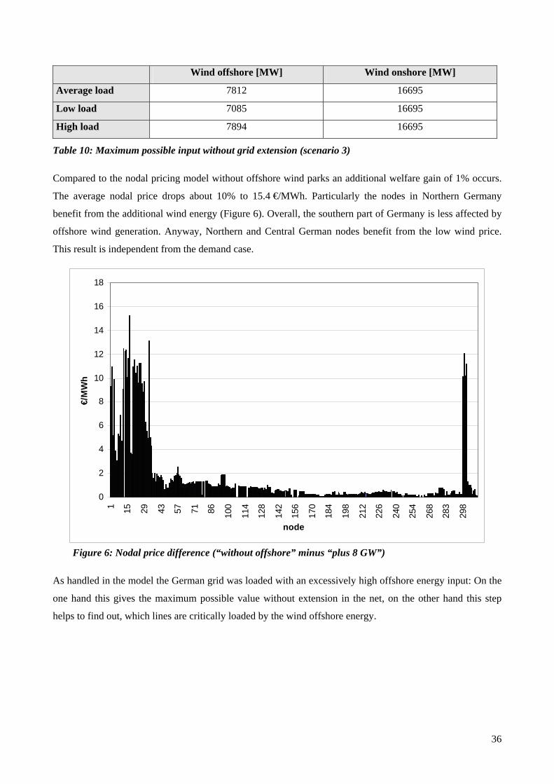
36

Wind offshore [MW] Wind onshore [MW]

Average load 7812 16695

Low load 7085 16695

High load 7894 16695

Table 10: Maximum possible input without grid extension (scenario 3)

Compared to the nodal pricing model without offshore wind parks an additional welfare gain of 1% occurs.

The average nodal price drops about 10% to 15.4 €/MWh. Particularly the nodes in Northern Germany

benefit from the additional wind energy (Figure 6). Overall, the southern part of Germany is less affected by

offshore wind generation. Anyway, Northern and Central German nodes benefit from the low wind price.

This result is independent from the demand case.

0

2

4

6

8

10

12

14

16

18

1 15 29 43 57 71 86 100

114

128

142

156

170

184

198

212

226

240

254

268

283

298

node

€/M

Wh

Figure 6: Nodal price difference (“without offshore” minus “plus 8 GW”)

As handled in the model the German grid was loaded with an excessively high offshore energy input: On the

one hand this gives the maximum possible value without extension in the net, on the other hand this step

helps to find out, which lines are critically loaded by the wind offshore energy.

37

Line Description From Bus To Bus

3 Wilhelmshaven to Conneforde 2 3

4 Conneforde to Emden 3 4

18 Dt. Bucht 1 to Dt. Bucht 2 298 299

27 Sottrum to Landsbergen 17 46

31 Dollern to Wister 18 21

46 Hamburg Hafen to Hamburg Ost 28 30

168 Rommerskirchen to Niederaußen 115 116

369 Neuenhagen to Marzahn 266 267

Table 11: Congested lines within the “plus 8 GW” scenario (average load)

4.2.3 Offshore model grid extension: scenario 4 vs. scenario 3

One scenario of German energy policy makers is to install offshore wind energy plants with up to 15 GW.

This study implemented a goal of 13 GW by building and upgrading electricity lines in the north of

Germany. Some of them have already been planned (VEG, 2001). Although this study applies a very

ambitious extension (Table 12), the maximum offshore capacity could not be raised higher than 13.3 GW.

The latter is caused by additional congestions in Northern Germany. The results show that a grid extension

has to be planned very carefully to maximize the additional benefits. Often new congestions appear in the

downstream grid limiting the effect of the extension.

From node To node Type of line

1. Emden Diele double 380 kV

2. Wilhelmshaven Conneforde double 380 kV

3. Diele Cloppenburg double 380 kV

4. Cloppenburg St. Hülfe double 380 kV

5. Emden Coneforde upgrade to 380kV

6. Cloppenburg Coneforde upgrade to 380kV

Table 12: Assumed grid extension

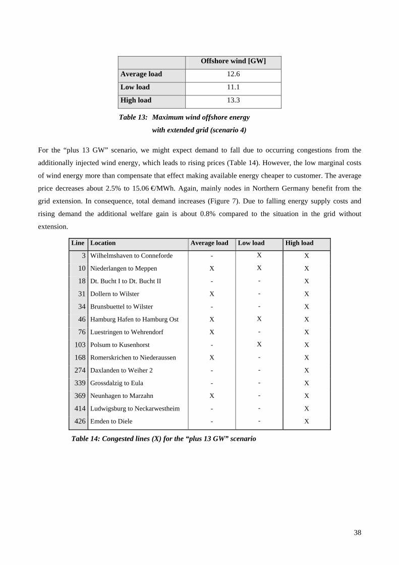
38

Offshore wind [GW]

Average load 12.6

Low load 11.1

High load 13.3

Table 13: Maximum wind offshore energy

with extended grid (scenario 4)

For the “plus 13 GW” scenario, we might expect demand to fall due to occurring congestions from the

additionally injected wind energy, which leads to rising prices (Table 14). However, the low marginal costs

of wind energy more than compensate that effect making available energy cheaper to customer. The average

price decreases about 2.5% to 15.06 €/MWh. Again, mainly nodes in Northern Germany benefit from the

grid extension. In consequence, total demand increases (Figure 7). Due to falling energy supply costs and

rising demand the additional welfare gain is about 0.8% compared to the situation in the grid without

extension.

Line Location Average load Low load High load

3 Wilhelmshaven to Conneforde - X X

10 Niederlangen to Meppen X X X

18 Dt. Bucht I to Dt. Bucht II - - X

31 Dollern to Wilster X - X

34 Brunsbuettel to Wilster - - X

46 Hamburg Hafen to Hamburg Ost X X X

76 Luestringen to Wehrendorf X - X

103 Polsum to Kusenhorst - X X

168 Romerskrichen to Niederaussen X - X

274 Daxlanden to Weiher 2 - - X

339 Grossdalzig to Eula - - X

369 Neunhagen to Marzahn X - X

414 Ludwigsburg to Neckarwestheim - - X

426 Emden to Diele - - X

Table 14: Congested lines (X) for the “plus 13 GW” scenario

39

0,00%

0,20%

0,40%

0,60%

0,80%

1,00%

1,20%

1,40%

1,60%

low average high

Dem

and

chan

ge

nodal plus 8 GW nodal plus 13 GW

Figure 7: Change in optimal demand: scenario “nodal price plus 8 GW” vs.

“nodal price plus 8 GW”

Surprisingly, some nodes have prices below their costs of generation. This is caused by the welfare

maximizing attempt. If additional demand at one node enables supply a node with a higher willingness to

pay, the welfare gain from this node can be higher than the loss from the first node. This phenomenon only

occurs in few cases in Northern Germany enabling a higher flow of cheap wind energy to the South.

However, due to these congestions some nodes face a serious price increase (Figure 8).

-20

-15

-10

-5

0

5

10

15

20

1 15 29 43 57 71 86 100

114

128

142

156

170

184

198

212

226

240

254

268

283

298

node

€/M

Wh

Figure 8: Nodal price difference (“plus 8 GW” minus “plus 13 GW”)

40

Since only a limited amount of wind energy can be transported to the demand centers in the south, only

Northern Germany would contribute to the welfare gain and benefit from the offshore wind input (Figure 9).

Moreover, it must be considered that thenetwork extension ivestments are not taken into account in the

welfare analysis. Further, grid constructions are likely to become political issues. Under these circumstances,

the welfare gain from grid extensions must be regarded differently to the welfare gain from introducing

nodal pricing. Because only a limited amount of wind energy can be transported to the demand centers in the

south, in a nodal pricing regime only Northern Germany would participate in the welfare gain resulting from

offshore wind. The analysis shows that the German electricity grid is not suited for a high amount of offshore

capacity. The highly meshed network rather seems to be designed for decentralized input.34

Figure 9: Congested lines around the North Sea 13 GW average 34 Note that, here, ‘decentralized’ refers to units significantly smaller than 8 GW.

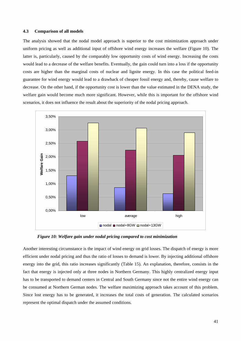
41

4.3 Comparison of all models

The analysis showed that the nodal model approach is superior to the cost minimization approach under

uniform pricing as well as additional input of offshore wind energy increases the welfare (Figure 10). The

latter is, particularly, caused by the comparably low opportunity costs of wind energy. Increasing the costs

would lead to a decrease of the welfare benefits. Eventually, the gain could turn into a loss if the opportunity

costs are higher than the marginal costs of nuclear and lignite energy. In this case the political feed-in

guarantee for wind energy would lead to a drawback of cheaper fossil energy and, thereby, cause welfare to

decrease. On the other hand, if the opportunity cost is lower than the value estimated in the DENA study, the

welfare gain would become much more significant. However, while this is important for the offshore wind

scenarios, it does not influence the result about the superiority of the nodal pricing approach.

0,00%

0,50%

1,00%

1,50%

2,00%

2,50%

3,00%

3,50%

low average high

Wel

fare

Gai

n

nodal nodal+8GW nodal+13GW

Figure 10: Welfare gain under nodal pricing compared to cost minimization

Another interesting circumstance is the impact of wind energy on grid losses. The dispatch of energy is more

efficient under nodal pricing and thus the ratio of losses to demand is lower. By injecting additional offshore

energy into the grid, this ratio increases significantly (Table 15). An explanation, therefore, consists in the

fact that energy is injected only at three nodes in Northern Germany. This highly centralized energy input

has to be transported to demand centers in Central and South Germany since not the entire wind energy can

be consumed at Northern German nodes. The welfare maximizing approach takes account of this problem.

Since lost energy has to be generated, it increases the total costs of generation. The calculated scenarios

represent the optimal dispatch under the assumed conditions.

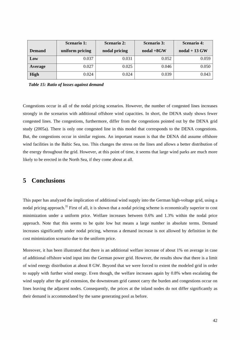
42

Demand

Scenario 1:

uniform pricing

Scenario 2:

nodal pricing

Scenario 3:

nodal +8GW

Scenario 4:

nodal + 13 GW

Low 0.037 0.031 0.052 0.059

Average 0.027 0.025 0.046 0.050

High 0.024 0.024 0.039 0.043

Table 15: Ratio of losses against demand

Congestions occur in all of the nodal pricing scenarios. However, the number of congested lines increases

strongly in the scenarios with additional offshore wind capacities. In short, the DENA study shows fewer

congested lines. The congestions, furthermore, differ from the congestions pointed out by the DENA grid

study (2005a). There is only one congested line in this model that corresponds to the DENA congestions.

But, the congestions occur in similar regions. An important reason is that the DENA did assume offshore

wind facilities in the Baltic Sea, too. This changes the stress on the lines and allows a better distribution of

the energy throughout the grid. However, at this point of time, it seems that large wind parks are much more

likely to be erected in the North Sea, if they come about at all.

5 Conclusions

This paper has analyzed the implication of additional wind supply into the German high-voltage grid, using a

nodal pricing approach.35 First of all, it is shown that a nodal pricing scheme is economically superior to cost

minimization under a uniform price. Welfare increases between 0.6% and 1.3% within the nodal price

approach. Note that this seems to be quite low but means a large number in absolute terms. Demand

increases significantly under nodal pricing, whereas a demand increase is not allowed by definition in the

cost minimization scenario due to the uniform price.

Moreover, it has been illustrated that there is an additional welfare increase of about 1% on average in case

of additional offshore wind input into the German power grid. However, the results show that there is a limit

of wind energy distribution at about 8 GW. Beyond that we were forced to extent the modeled grid in order

to supply with further wind energy. Even though, the welfare increases again by 0.8% when escalating the

wind supply after the grid extension, the downstream grid cannot carry the burden and congestions occur on

lines leaving the adjacent nodes. Consequently, the prices at the inland nodes do not differ significantly as

their demand is accommodated by the same generating pool as before.

43

Note as well that the 8 GW boundary for the current grid already includes that only offshore wind facilities

generate in Northern Germany, whereas existing large-scale plants would not be dispatched. However, these

facilities might be necessary for balancing and response power. Problems may arise, if the construction of

offshore wind mills sets negative incentives for investments in other types of generation plants. This is not

represented in our straightforward marginal consideration.

References

Alaywan, Ziad, and Tong Wu (2004): Transitioning the California Market from a Zonal to a Nodal

Framework: An Operational Perspective. In: Proceedings of the Power Systems Conference and

Exposition, 2, 862-867. Retrieved September 01, 2005, from

http://www.caiso.com/docs/09003a6080/32/2c/09003a6080322c6d.pdf

Bohn, Roger E., Caramanis, Michael C., and Fred C. Schweppe (1984): Optimal pricing in electrical

networks over space and time. In: Rand Journal of Economics, 15, 360-375.

Borenstein, Severin, Bushnell, James, and Frank Wolak (2000): Diagnosing Market Power in California’s

Deregulated Wholesale Electricity Market. PWP-064, University of California Energy Institute.

Retrieved September 01, 2005, from http://www.ucei.berkeley.edu/ucei/PDF/pwp064.pdf

Bower, John (2004): Electricity Infrastructure & Security of Supply: Should EU Governments Invest in

Transmission Capacity? Oxford Institute for Energy Studies. Retrieved August 31, 2005, from

http://www.oxfordenergy.org/comment_prn.php?0403

CAISO (2005): Market Redesign and Technology Upgrade. Locational Marginal Pricing (LMP) Study 3B.

Retrieved August 31, 2005, from http://www.caiso.com/docs/2005/08/24/2005082414133610519.pdf

Chen, Luonan, Suzuki, H., Wachi, T., and Y. Shimura (2002): Components of nodal prices for electric power

systems. In: IEEE Transactions on Power Systems, 17, 41-49.

DENA (2005a): dena-Netzstudie, Energiewirtschaftliche Planung für die Netzintegration von Windenergie in

Deutschland an Land und Offshore bis zum Jahr 2020. Deutsche Energie-Agentur.

DENA (2005b): Summary of the Essential Results, Planning of the Grid Integration of Wind Energy in

Germany Onshore and Offshore up to the Year 2020 (dena Grid study). Deutsche Energie-Agentur.

DESTATIS (2005): Statistik regional 2004. Statistisches Bundesamt Deutschland. Retrieved July 21, 2005,

from http://www.destatis.de/allg/d/veroe/proser211_d.htm.

DEWI (2005): Deutschlands Windindustrie bleibt Weltmeister. Deutsches Windenergie-Institut. Retrieved

September 06, 2005, from www.dewi.de/dewi_neu/deutsch/themen/statistic/pdf/pm28072005.pdf.

35 Note that we did not consider the case without onshore wind energy availability. Balancing and response power are regarded to exist to a sufficient degree and cause marginal costs that are, here, referred to as opportunity costs for wind.

44

Ding, Feng, and J. David Fuller (2005): Nodal, Uniform, or Zonal Pricing: Distribution of Economic

Surplus. In: IEEE Transactions on Power Systems, 20, 875-882. Retrieved September 01, 2005, from

http://ieeexplore.ieee.org/iel5/59/30784/01425584.pdf?arnumber=1425584

E.On Netz AG (2005): Netznutzungsentgelte für die Netznutzung das Stromversorgungsnetz der E.ON Netz

GmbH. Retrieved August 29, 2005, from http://www.eon-

netz.com/Ressources/downloads/netznutzungsentgelte.de.pdf.

EIA (2004): Electric power Annual 2003. Energy Information Administration. Retrieved September 06,

2005, from http://www.eia.doe.gov/cneaf/electricity/epa/epa.pdf.

EnBW AG (2005): Preisblätter Netznutzung. Retrieved August 29, 2005, from

http://www.enbw.com/content/de/netznutzer/strom/netznutzung/preisblaetter.

Energyquote (2005): UK Market Bulletin 13th April 2005. Retrieved August 31, 2005, from

http://www.energyquote.co.uk/markets/news_commentary.html

Fuller, J. David. (2004): Uniform, Nodal and Zonal Pricing in Electricity Markets. University of Waterloo,

Department of Management Sciences. Retrieved August 31, 2005, from

http://www.gerad.ca/fichiers/congres/2004-05-07-Fuller.pdf

Green, Richard (2004): Electricity Transmission Pricing: How Much does it Cost to Get it Wrong?

University of Hull Business School.

Hogan, William W. (1998): Transmission Investment and Competitive Electricity Markets. Harvard

University, John F. Kennedy School of Government, Center for Business and Government.

Hogan, William W. (1999): Transmission Congestion: The Nodal-Zonal Debate Revisited. Harvard

University, John F. Kennedy School of Government, Center for Business and Government. Retrieved

August 29, 2005, from http://ksghome.harvard.edu/~whogan/nezn0227.pdf

Hsu, Michael (1997): An Introduction to the Pricing of Electric Power Transmission. In: Utilities Policy, 6,

257-270.

Johnsen, Tor Arnt, Verma, Shashi Kant, and Catherine Wolfram (1999): Zonal Pricing and Demand-Side

Bidding in the Norwegian Electricity Market. PWP-063, University of California Energy Institute.

Retrieved September 01, 2005, from http://www.ucei.berkeley.edu/ucei/PDF/pwp063.pdf

Koettnitz, Harald, and Hans Pundt (1967): Berechnung elektrischer Energieversorgungsnetze, Band I:

Mathematische Grundlagen und Netzparameter. Leipzig, VEB Deutscher Verlag für

Grundstoffindustrie.

Koettnitz, Harald, Winkler, Gert, and Klaus-Dieter Weßnigk (1986): Grundlagen elektrischer

Betriebsvorgänge in Elektroenergiesystemen. Leipzig, VEB Deutscher Verlag für Grundstoffindustrie.

Krause, Thilo (2005): Congestion Management in Liberalized Electricity Markets – Theoretical Concepts

and International Application. EEH – power systems laboratory, Swiss Federal Institute of

Technology Zurich. Retrieved August 31, 2005, from

http://www.eeh.ee.ethz.ch/downloads/psl/publications/krause_congestion_management.pdf

Lunze, Klaus (1987): Berechnung elektrischer Stromkreise. Berlin, VEB Verlag Technik.

45

Ma, Xingwang, Sun, David I., and Kwok W. Cheung (2003): Evolution Toward Standardized Market

Design. In: IEEE Transactions on Power Systems, 18, 460-469. Retrieved September 01, 2005, from

http://ieeexplore.ieee.org/iel5/59/26968/01198273.pdf?isnumber=&arnumber=1198273

Overbye, Thomas J., Cheng, Xu, and Yan Sun (2004): A Comparison of the AC and DC Power Flow Models

for LMP Calculations. In: Proceedings of the 37th Hawaii International Conference on System

Sciences 2004.

Pfaffenberger, Wolfgang, and Maren Hille (2004): Investitionen im liberalisierten Energiemarkt: Optionen,

Marktmechanismen, Rahmenbedingungen. Final Report, University of Bremen, Bremer Energie

Institut.

Pundt, Hans (1983): Elektroenergiesysteme: 5. Lehrbrief. Zwickau, Zentralstelle für Lehr- und

Organisationsmittel des Ministeriums für Bildung.

Pundt, Hans, and Peter Schegner (1997): Wissensspeicherheft: Elektroenergiesysteme. Dresden University of

Technology, Institute for Electrical Power Supply.

RWE AG (2005a): Facts & Figures 2005. Retrieved September 01, 2005, from

http://www2.rwecom.geber.at/factbook/en/servicepages/downloads/files/electricity_grid_rwe_fact.pdf.

RWE AG (2005b): Preise für die Nutzung des Netzes der RWE Transportnetz Strom GmbH. Retrieved

August 29, 2005, from http://www.rwe-

transportnetzstrom.com/generator.aspx/netznutzung/netznutzungspreise/language=de/id=75492/netznu

tzungspreise-home.html.

Schröter, Jochen (2004): Auswirkungen des europäischen Emissionshandelssystems auf den

Kraftwerkseinsatz in Deutschland. Diploma thesis, Berlin University of Technology, Institute of

Power Engineering. Retrieved September 01, 2005, from

http://basis.gruene.de/bag.energie/papiere/eeg_diplarbeit_schroeter_lang.pdf.

Schweppe, Fred C., Caramanis, Michael C., Tabors, Richard D., and Roger E. Bohn (1988): Spot Pricing Of

Electricity. Boston, Kluwer.

Stigler, Heinz, and Christian Todem (2005): Optimization of the Austrian Electricity Sector (Control Zone of

VERBUND APG) under the Constraints of Network Capacities by Nodal Pricing. In: Central

European Journal of Operations Research, 13, 105-125.

Statistik-Portal: Volkswirtschaftliche Gesamtrechnungen. Bruttoinlandsprodukt. Retrieved June 23, 2005,

from http://www.statistik-portal.de/Statistik-Portal/de_jb27_jahrtab65.asp

Stoft, Steven (2002): Power System Economics: Designing Markets for Electricity. Piscataway, NJ, IEEE

Press, Wiley-Interscience.

Todem, Christian (2004): Methoden und Instrumente zur gesamtsystemischen Analyse und Optimierung

konkreter Problemstellungen im liberalisierten Elektrizitätsmarkt. Dissertation, Graz University of

Technology, Department of Electricity Economics and Energy Innovation.

Todem, Christian, Stigler, Heinz, Huber, Christoph, Wulz, Christoph, and Hannes Wornig (2004): Nodal

Pricing als Analyseinstrumentarium zur Untersuchung der volkswirtschaftlichen Auswirkungen eines

46

marktbasierten Engpassmanagements bei Engpässen im Verbundsystem. Graz University of

Technology, Department of Electricity Economics and Energy Innovation.

Törnquist, Jonas (2005): UK Transmission System Challenges. The Office of Gas and Electricity Markets.

Retrieved September 01, 2005, from http://www.iea.org/textbase/work/2004/transmission/tornquist.pdf

UCTE (2004): Interconnected Network of UCTE. Dortmund, Abel Druck.

VDN (2001): Verbändevereinbarung über Kriterien zur Bestimmung von Netznutzungsentgelten für

elektrische Energie und über Prinzipien der Netznutzung, 13.12.2001. Retrieved August 29, 2005,

from http://www.vdn-berlin.de/verbaendevereinbarung_ii_plus.asp

VDN (2005): Jahreshöchstlast Strom 2004 im europäischen Vergleich. Retrieved August 20, 2005, from

http://www.vdn-berlin.de/akt_jhoechstlast_2005_07_28.asp.

VGE (2000): Elektrizitäts-Verbundsysteme in Deutschland. Essen, Verlag Glückauf.

VGE (2005): Jahrbuch der europäischen Energie- und Rohstoffwirtschaft 2005. Essen,Verlag Glückauf

GmbH.

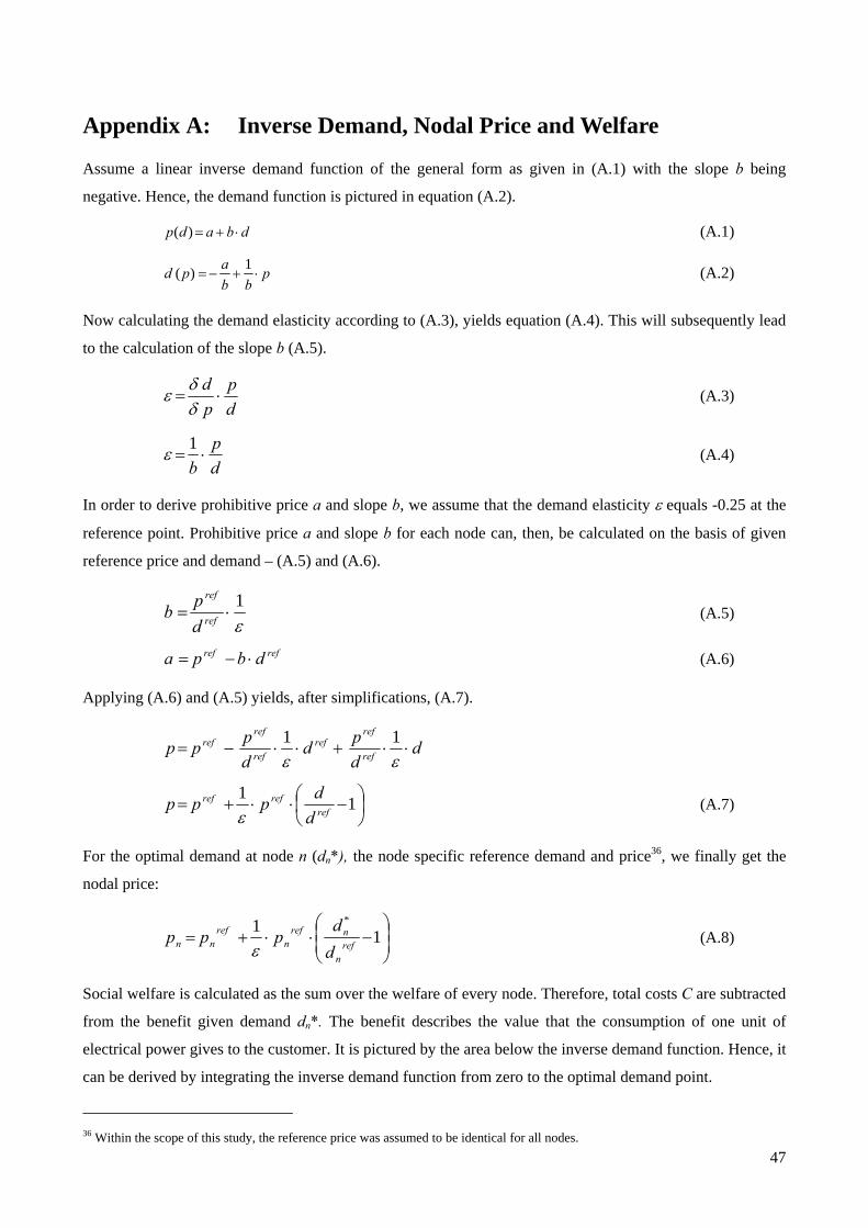
47

Appendix A: Inverse Demand, Nodal Price and Welfare

Assume a linear inverse demand function of the general form as given in (A.1) with the slope b being

negative. Hence, the demand function is pictured in equation (A.2).

dbadp ⋅+=)( (A.1)

pbb

apd ⋅+−=1)( (A.2)

Now calculating the demand elasticity according to (A.3), yields equation (A.4). This will subsequently lead

to the calculation of the slope b (A.5).

dp

pd

⋅=δδε (A.3)

dp

b⋅=

1ε (A.4)

In order to derive prohibitive price a and slope b, we assume that the demand elasticity ε equals -0.25 at the

reference point. Prohibitive price a and slope b for each node can, then, be calculated on the basis of given

reference price and demand – (A.5) and (A.6).

ε1

⋅= ref

ref

dpb (A.5)

refref dbpa ⋅−= (A.6)

Applying (A.6) and (A.5) yields, after simplifications, (A.7).

ddpd

dppp ref

refref

ref

refref ⋅⋅+⋅⋅−=

εε11

⎟⎠⎞

⎜⎝⎛ −⋅⋅+= 11

refrefref

ddppp

ε (A.7)

For the optimal demand at node n (dn*), the node specific reference demand and price36, we finally get the

nodal price:

⎟⎟⎠

⎞⎜⎜⎝

⎛−⋅⋅+= 11 *

refn

nrefn

refnn d

dppp

ε (A.8)

Social welfare is calculated as the sum over the welfare of every node. Therefore, total costs C are subtracted

from the benefit given demand dn*. The benefit describes the value that the consumption of one unit of

electrical power gives to the customer. It is pictured by the area below the inverse demand function. Hence, it

can be derived by integrating the inverse demand function from zero to the optimal demand point.

36 Within the scope of this study, the reference price was assumed to be identical for all nodes.

48

∑ ∫∫ ⎟⎟

⎠

⎞

⎜⎜

⎝

⎛−=

n

d

nnn

d

nn

nn

dddcdddpdW**

0

***

0

*** )()()( (A.9)

( )∑⎥⎥⎦

⎤

⎢⎢⎣

⎡⎟⎟⎠

⎞⎜⎜⎝

⎛⋅+−=

nrefn

refn

nnrefn d

pddp

εε1

21)11( 2** - C

49

Appendix B: Implementing the optimization problem in GAMS

First part

As for the scalars, Nodes, N and NN denote all the nodes form no. 1 to no. 308. Similarly all the lines from

no. 1 to no. 407 are represented by Line, L or LL. With the scalars MVABase, VoltageBase1 and

VoltageBase2, which are values of apparent power, first and second voltage level respectively, the

normalization bases ZBase1 and ZBase2 are computed. They are needed in the next part. In addition a fixed

demand elasticity ε for all demand functions is given as a scalar.

Second part

Almost all parameters are imported directly from excel sheets without conversion:

FromBus(L) and ToBus(L) are the numbers of the starting node and the end node linked directly with

each other by a line.

LineVoltage(L) is the voltage level of a line.

ThermalLimit(L), as mentioned above, is the maximum current through a line without overheating

and damaging the line.

Demand0(N) is the reference demand of power at a node.

Price0(N) is the reference price at a node.

There are nine types of power stations in this model. Each of them has a maximum supply capacity per node.

This is memorised in Max_Generation_[name](N) whereas name is the short name for the type of power

station. Except wind stations, each type of power station has different marginal costs of production that are

denoted MC_[name](N) whereas name is again the short name of the power station type. The opportunity

cost of wind supply are memorised in OC_wind(N).

Some parameters are converted:

The given resistances and reactances of the lines are divided by ZBase1 or ZBase2 to get the normalized

parameters Resistance(L) and Reactance(L). As a result both parameters are expressed in a per unit system.

The maximum possible load flow through a line for thermal reasons is calculated with (1) and memorised in

parameter PowerFlowLimit(L).

PowerFlowLimit(L) = 3 * LineVoltage(L) *ThermalLimit(L) (1)

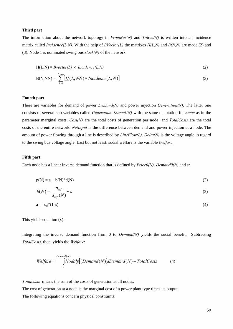
50

Third part

The information about the network topology in FromBus(N) and ToBus(N) is written into an incidence

matrix called Incidence(L,N). With the help of BVector(L) the matrixes H(L,N) and B(N,N) are made (2) and

(3). Node 1 is nominated swing bus slack(N) of the network.

H(L,N) = Bvector(L) × Incidence(L,N) (2)

B(N,NN) = [ ]∑=

∗max

1),(),(

L

LNLIncidenceNNLH (3)

Fourth part

There are variables for demand of power Demand(N) and power injection Generation(N). The latter one

consists of several sub variables called Generation_[name](N) with the same denotation for name as in the

parameter marginal costs. Cost(N) are the total costs of generation per node and TotalCosts are the total

costs of the entire network. NetInput is the difference between demand and power injection at a node. The

amount of power flowing through a line is described by LineFlow(L). Delta(N) is the voltage angle in regard

to the swing bus voltage angle. Last but not least, social welfare is the variable Welfare.

Fifth part

Each node has a linear inverse demand function that is defined by Price0(N), Demand0(N) and ε:

p(N) = a + b(N)*d(N) (2)

ε∗=)(

)(Nd

pNb

ref

ref (3)

a = pref*(1-ε) (4)

This yields equation (x).

Integrating the inverse demand function from 0 to Demand(N) yields the social benefit. Subtracting

TotalCosts, then, yields the Welfare:

[ ] TotalCostsNdDemandNDemandNodalpWelfareNDemand

−= ∫ )()(()(

0

(4)

Totalcosts means the sum of the costs of generation at all nodes.

The cost of generation at a node is the marginal cost of a power plant type times its output.

The following equations concern physical constraints:

51

For a network without losses NetInput equals B times Delta for all nodes. Losses are calculated with the

second summand and are added to the nodes at the ends of a line in equal shares. (5)

LineFlow is H times Delta. (6)

NetInput(N) = ∑=

∗max

1

)(),(N

NN

NNDeltaNNNB ∗ MVABase

+ 0,5 ∑=

∗max

1

N

N

Resistance(L) ( )2),()( NLIncidenceLLineFlow ∗∗ (5)

LineFlow(L) = ∑=

∗max

1)(),(

N

NNDeltaNLH (6)

The modulus of LineFlow faces an upper bound. (7a) (7b)

The Delta is fixed at 0 for the swing bus. (8)

No power injection of a power plant type is allowed to exceed its maximum capacity of generation. (9)

LineFlow(L) ∗ MVABase ≤ PowerFlowLimit(L) (7a)

LineFlow(L) ∗ MVABase ≥ - PowerFlowLimit(L) (7b)

Slack(N) ∗ Delta(N) = 0 (8)

Generation_type(N) =L= Max_Generation_type(N) (9)

Spreadsheet: Parameters

Name Schweppe`s notation description

BVector(L) Ω

Incidence(L,N) A incidence matrix: line-nodes

identity

H(L,N) Ω *A transfer matrix for calculation

[p.u.]

B(N,N) AT* Ω *A system susceptance matrix

[p.u.]

LineVoltage(L) voltage level of a line [kV]

ThermalLimit(L) maximum possible current [A]

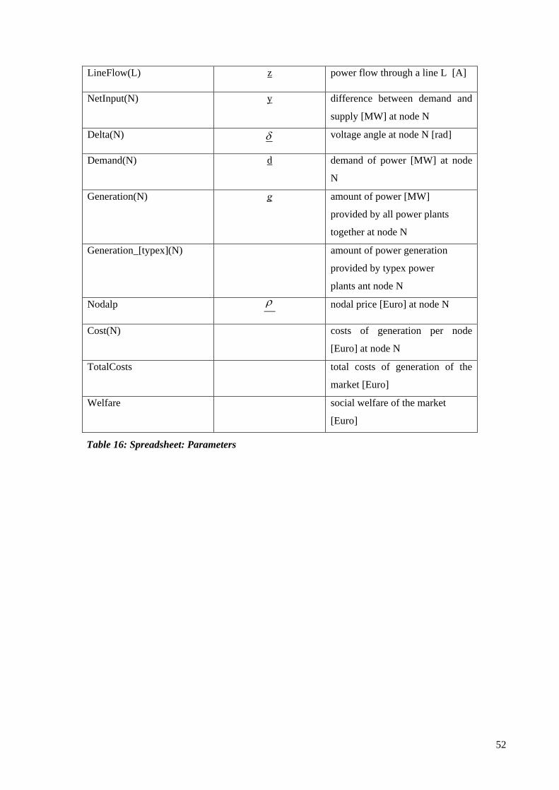
52

LineFlow(L) z power flow through a line L [A]

NetInput(N) y difference between demand and

supply [MW] at node N

Delta(N) δ voltage angle at node N [rad]

Demand(N) d demand of power [MW] at node

N

Generation(N) g amount of power [MW]

provided by all power plants

together at node N

Generation_[typex](N) amount of power generation

provided by typex power

plants ant node N

Nodalp ρ nodal price [Euro] at node N

Cost(N) costs of generation per node

[Euro] at node N

TotalCosts total costs of generation of the

market [Euro]

Welfare social welfare of the market

[Euro]

Table 16: Spreadsheet: Parameters

53

Appendix C: Assumptions for calculating transmission losses in the

DCLF

According to Todem (2004, pp.130-131), transmission losses are made up by the sum of the load flows along

a line. Those can flow in both directions, so that:

kjjkjk PP L += (C.1)

Furthermore it can be stated that:

kjjki GG G == (C.2)

kjjki BB B == (C.3)

kjΘ=Θ sin- sin jk (C.4)

kjΘ=Θ cos cos jk (C.5)

Under the assumptions that

ii R X ff (C.6)

one can insert equation (3.10) into (C.1) and then simplify the resulting equation by inserting equations

(3.16), (3.17), (C.2), (C.3), (C.4) and (C.5). These steps lead to the equation for estimating transmission

losses (3.18).

54

Appendix D: Result data

0

2

4

6

8

10

12

14

16

18

20

1 15 29 43 57 71 86 100

114

128

142

156

170

184

198

212

226

240

254

268

283

298

Node

€/M

Wh

Figure 11: Nodal prices without offshore wind (low load)

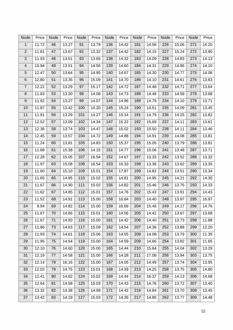
55

Node Price Node Price Node Price Node Price Node Price Node Price Node Price

1 11.72 46 13.27 91 13.79 136 14.42 181 14.56 226 15.06 271 14.20

2 11.81 47 13.67 92 13.32 137 14.42 182 14.15 227 15.24 272 13.90

3 11.93 48 13.51 93 13.65 138 14.32 183 14.09 228 14.83 273 14.13

4 10.94 49 13.51 94 14.56 139 14.60 184 14.31 229 14.86 274 14.10

5 12.47 50 13.64 95 14.95 140 14.67 185 14.30 230 14.77 275 14.08

6 12.80 51 13.35 96 15.09 141 14.70 186 14.10 231 14.61 276 13.63

7 12.22 52 13.29 97 15.17 142 14.72 187 14.48 232 14.71 277 13.64

8 11.83 53 13.30 98 14.08 143 14.73 188 14.48 233 14.58 278 13.68

9 11.92 54 13.27 99 14.07 144 14.96 189 14.79 234 14.10 279 13.71

10 11.87 55 13.42 100 14.20 145 15.24 190 14.51 235 14.09 281 13.45

11 11.91 56 13.29 101 14.27 146 15.14 191 14.79 236 14.25 282 13.82

12 12.52 57 13.09 102 14.34 147 15.22 192 15.69 237 14.11 283 13.61

13 12.36 58 13.74 103 14.47 148 15.02 193 15.50 238 14.11 284 13.46

14 12.45 59 13.57 104 14.72 149 14.88 194 14.91 239 14.08 285 13.81

15 11.24 60 13.81 105 14.83 150 15.37 195 15.05 240 13.79 286 13.81

16 11.68 61 15.38 106 14.15 151 14.77 196 15.06 241 13.48 287 13.71

17 12.28 62 15.05 107 16.54 152 14.67 197 13.33 242 13.52 288 13.32

18 11.97 63 15.08 108 16.54 153 16.33 198 13.36 243 13.62 289 13.35

19 11.60 64 15.10 109 15.01 154 17.87 199 14.82 244 13.51 290 13.34

20 11.65 65 14.95 110 15.02 155 14.81 200 14.95 245 14.21 292 14.30

21 11.67 66 14.90 111 15.02 156 14.82 201 15.46 246 13.75 293 14.33

22 11.62 67 14.85 112 15.01 157 14.76 202 15.43 247 13.91 294 14.43

23 11.52 68 14.91 113 15.00 158 16.84 203 14.40 248 13.97 295 16.97

24 9.94 69 14.82 114 15.00 159 16.69 204 15.46 249 14.17 296 14.76

25 11.67 70 14.66 115 15.01 160 14.56 205 14.42 250 13.67 297 13.68

26 11.67 71 14.93 116 15.00 161 14.42 206 14.40 251 13.73 298 11.88

27 11.86 73 14.63 117 15.09 162 14.54 207 14.36 252 13.88 299 12.20

28 11.93 74 14.61 118 15.06 163 14.55 208 14.08 253 13.79 300 11.35

29 11.95 75 14.64 119 15.00 164 14.59 209 14.66 254 13.82 301 11.65

30 12.10 76 14.60 120 15.00 165 14.44 210 15.64 255 14.04 302 13.29

31 12.19 77 14.58 121 15.00 166 14.28 211 17.08 256 13.94 303 13.75

32 12.14 78 16.16 122 15.00 167 14.05 212 14.49 257 13.74 304 13.95

33 12.02 79 14.75 123 15.01 168 14.39 213 14.25 258 13.75 305 14.80

34 12.41 80 14.62 124 15.02 169 14.44 214 16.37 259 14.13 306 14.68

35 12.64 81 14.58 125 15.03 170 14.43 215 14.76 260 13.72 307 13.40

36 13.32 82 14.38 126 14.99 171 14.42 216 14.84 261 13.70 308 13.45

37 13.42 83 14.19 127 15.03 172 14.35 217 14.80 262 13.77 309 14.48

56

38 13.36 84 14.31 128 15.04 173 14.37 218 14.62 263 13.71 310 14.67

39 13.48 85 13.51 129 15.04 174 14.94 219 14.61 264 13.58 40 13.60 86 13.55 130 15.02 175 14.87 220 14.93 265 13.79 41 13.84 87 13.84 131 14.85 176 14.44 221 14.98 266 13.91 42 13.80 88 13.79 132 15.53 177 14.72 222 15.46 267 14.21 43 14.07 89 13.78 133 14.10 178 14.71 223 15.07 268 14.26 44 13.34 90 13.74 134 15.28 179 14.72 224 14.79 269 14.23 45 13.89 135 14.49 180 14.69 225 14.79 270 14.22

Table 17: Prices per node: without offshore wind (low load)

57

0

5

10

15

20

25

30

35

40

45

1 15 29 43 57 71 86 100

114

128

142

156

170

184

198

212

226

240

254

268

283

298

Node

€/M

Wh

Figure 12: Nodal prices without offshore wind (high load)

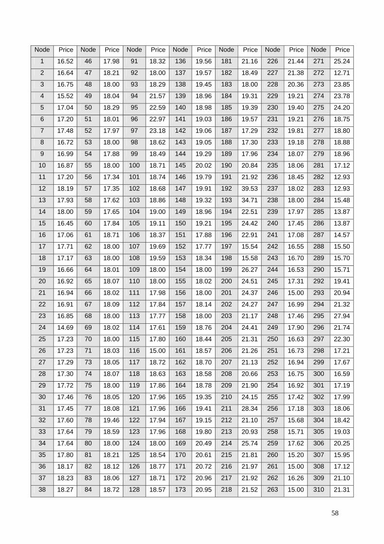
58

Node Price Node Price Node Price Node Price Node Price Node Price Node Price

1 16.52 46 17.98 91 18.32 136 19.56 181 21.16 226 21.44 271 25.24

2 16.64 47 18.21 92 18.00 137 19.57 182 18.49 227 21.38 272 12.71

3 16.75 48 18.00 93 18.29 138 19.45 183 18.00 228 20.36 273 23.85

4 15.52 49 18.04 94 21.57 139 18.96 184 19.31 229 19.21 274 23.78

5 17.04 50 18.29 95 22.59 140 18.98 185 19.39 230 19.40 275 24.20

6 17.20 51 18.01 96 22.97 141 19.03 186 19.57 231 19.21 276 18.75

7 17.48 52 17.97 97 23.18 142 19.06 187 17.29 232 19.81 277 18.80

8 16.72 53 18.00 98 18.62 143 19.05 188 17.30 233 19.18 278 18.88

9 16.99 54 17.88 99 18.49 144 19.29 189 17.96 234 18.07 279 18.96

10 16.87 55 18.00 100 18.71 145 20.02 190 20.84 235 18.06 281 17.12

11 17.20 56 17.34 101 18.74 146 19.79 191 21.92 236 18.45 282 12.93

12 18.19 57 17.35 102 18.68 147 19.91 192 39.53 237 18.02 283 12.93

13 17.93 58 17.62 103 18.86 148 19.32 193 34.71 238 18.00 284 15.48

14 18.00 59 17.65 104 19.00 149 18.96 194 22.51 239 17.97 285 13.87

15 16.45 60 17.84 105 19.11 150 19.21 195 24.42 240 17.45 286 13.87

16 17.06 61 18.71 106 18.37 151 17.88 196 22.91 241 17.08 287 14.57

17 17.71 62 18.00 107 19.69 152 17.77 197 15.54 242 16.55 288 15.50

18 17.17 63 18.00 108 19.59 153 18.34 198 15.58 243 16.70 289 15.70

19 16.66 64 18.01 109 18.00 154 18.00 199 26.27 244 16.53 290 15.71

20 16.92 65 18.07 110 18.00 155 18.02 200 24.51 245 17.31 292 19.41

21 16.94 66 18.02 111 17.98 156 18.00 201 24.37 246 15.00 293 20.94

22 16.91 67 18.09 112 17.84 157 18.14 202 24.27 247 16.99 294 21.32

23 16.85 68 18.00 113 17.77 158 18.00 203 21.17 248 17.46 295 27.94

24 14.69 69 18.02 114 17.61 159 18.76 204 24.41 249 17.90 296 21.74

25 17.23 70 18.00 115 17.80 160 18.44 205 21.31 250 16.63 297 22.30

26 17.23 71 18.03 116 15.00 161 18.57 206 21.26 251 16.73 298 17.21

27 17.29 73 18.05 117 18.72 162 18.70 207 21.13 252 16.94 299 17.67

28 17.30 74 18.07 118 18.63 163 18.58 208 20.66 253 16.75 300 16.59

29 17.72 75 18.00 119 17.86 164 18.78 209 21.90 254 16.92 301 17.19

30 17.46 76 18.05 120 17.96 165 19.35 210 24.15 255 17.42 302 17.99

31 17.45 77 18.08 121 17.96 166 19.41 211 28.34 256 17.18 303 18.06

32 17.60 78 19.46 122 17.94 167 19.15 212 21.10 257 15.68 304 18.42

33 17.64 79 18.59 123 17.96 168 19.80 213 20.93 258 15.71 305 19.03

34 17.64 80 18.00 124 18.00 169 20.49 214 25.74 259 17.62 306 20.25

35 17.80 81 18.21 125 18.54 170 20.61 215 21.81 260 15.20 307 15.95

36 18.17 82 18.12 126 18.77 171 20.72 216 21.97 261 15.00 308 17.12

37 18.23 83 18.06 127 18.71 172 20.96 217 21.92 262 16.26 309 21.10

38 18.27 84 18.72 128 18.57 173 20.95 218 21.52 263 15.00 310 21.31

59

39 18.36 85 17.59 129 18.77 174 24.48 219 21.49 264 16.49 40 18.18 86 17.75 130 19.01 175 24.27 220 21.65 265 14.20 41 18.42 87 18.33 131 17.89 176 21.06 221 21.57 266 12.50 42 18.69 88 18.31 132 20.30 177 21.43 222 22.87 267 27.89 43 18.97 89 18.30 133 18.45 178 21.39 223 21.72 268 27.43 44 18.15 90 18.27 134 18.55 179 21.43 224 21.00 269 27.15 45 18.60 135 19.26 180 21.33 225 20.64 270 26.40

Table 18: Prices per node: without offshore wind (high load)

60

0

5

10

15

20

25

1 15 29 43 57 71 86 100

114

128

142

156

170

184

198

212

226

240

254

268

283

298

Node

€/M

Wh

Figure 13: Nodal prices “plus 8 GW” (average load)

61

Node Price Node Price Node Price Node Price Node Price Node Price Node Price

1 5.63 46 16.01 91 16.26 136 17.36 181 17.85 226 18.19 271 17.72

2 4.05 47 16.11 92 15.37 137 17.37 182 17.36 227 18.39 272 14.69

3 10.00 48 16.14 93 15.78 138 17.48 183 17.29 228 17.70 273 17.33

4 4.05 49 16.13 94 17.42 139 17.25 184 17.56 229 16.88 274 17.30

5 11.75 50 15.93 95 18.08 140 17.17 185 17.55 230 16.99 275 17.46

6 12.78 51 15.12 96 18.32 141 17.12 186 17.35 231 16.84 276 15.49

7 10.35 52 15.17 97 18.45 142 17.16 187 17.15 232 17.15 277 15.52

8 10.00 53 15.32 98 16.30 143 17.25 188 17.16 233 16.87 278 15.58

9 8.43 54 14.78 99 16.29 144 17.45 189 17.66 234 16.10 279 15.62

10 10.45 55 14.86 100 16.47 145 18.06 190 17.83 235 16.09 281 15.09

11 6.39 56 14.22 101 16.52 146 17.90 191 18.30 236 16.42 282 14.71

12 4.06 57 13.64 102 16.59 147 18.00 192 19.51 237 16.11 283 14.51

13 3.98 58 14.71 103 16.83 148 17.48 193 19.43 238 16.11 284 14.84

14 4.02 59 14.82 104 16.91 149 17.18 194 18.50 239 16.09 285 14.85

15 4.56 60 15.21 105 16.97 150 17.61 195 18.80 240 15.62 286 14.86

16 3.58 61 16.75 106 16.14 151 16.38 196 18.76 241 15.06 287 14.92

17 0.70 62 16.25 107 18.05 152 16.28 197 15.41 242 15.00 288 14.73

18 11.64 63 16.26 108 18.00 153 17.39 198 15.46 243 15.12 289 14.80

19 11.29 64 16.25 109 16.03 154 18.00 199 18.47 244 15.02 290 14.79

20 4.05 65 16.12 110 16.02 155 16.92 200 18.62 245 15.54 292 17.54

21 3.51 66 16.11 111 16.01 156 16.93 201 19.83 246 15.00 293 17.71

22 4.59 67 16.11 112 15.89 157 16.98 202 19.76 247 15.39 294 17.90

23 3.88 68 16.11 113 15.83 158 18.00 203 17.83 248 15.77 295 22.17

24 3.37 69 16.06 114 15.68 159 18.25 204 19.84 249 16.08 296 18.16

25 3.96 70 15.94 115 15.85 160 17.10 205 17.87 250 15.31 297 16.59

26 3.96 71 16.09 116 15.00 161 16.95 206 17.85 251 15.39 298 5.31

27 5.81 73 16.03 117 16.58 162 17.10 207 17.76 252 15.56 299 3.89

28 6.56 74 16.04 118 16.52 163 17.11 208 17.41 253 15.43 300 4.60

29 5.92 75 16.00 119 15.92 164 17.76 209 18.20 254 15.52 301 3.95

30 9.20 76 16.05 120 16.01 165 17.71 210 19.70 255 15.95 302 15.31

31 10.00 77 16.03 121 16.01 166 17.54 211 22.41 256 15.79 303 16.21

32 10.69 78 17.71 122 16.00 167 17.29 212 17.67 257 15.14 304 16.19

33 2.60 79 16.43 123 16.01 168 17.62 213 17.47 258 15.16 305 16.92

34 10.78 80 16.07 124 16.05 169 17.79 214 20.87 259 16.09 306 17.89

35 11.66 81 16.16 125 16.46 170 17.80 215 18.17 260 15.00 307 14.87

36 14.47 82 15.95 126 16.61 171 17.79 216 18.26 261 14.95 308 15.10

37 14.79 83 15.83 127 16.69 172 17.74 217 18.24 262 15.33 309 17.83

38 14.54 84 16.44 128 16.49 173 17.76 218 18.02 263 14.98 310 17.98

39 15.00 85 15.42 129 16.67 174 18.60 219 18.00 264 15.14

62

40 15.11 86 15.56 130 17.09 175 18.47 220 18.26 265 14.90 41 15.73 87 16.22 131 16.15 176 17.81 221 18.27 266 14.65 42 15.77 88 16.23 132 17.99 177 18.06 222 19.10 267 18.31 43 16.10 89 16.24 133 16.23 178 18.03 223 18.24 268 18.24 44 14.91 90 16.23 134 16.42 179 18.06 224 17.77 269 18.16 45 16.15 135 16.88 180 18.00 225 17.59 270 18.00

Table 19: Prices per node: “plus 8 GW” (average load)

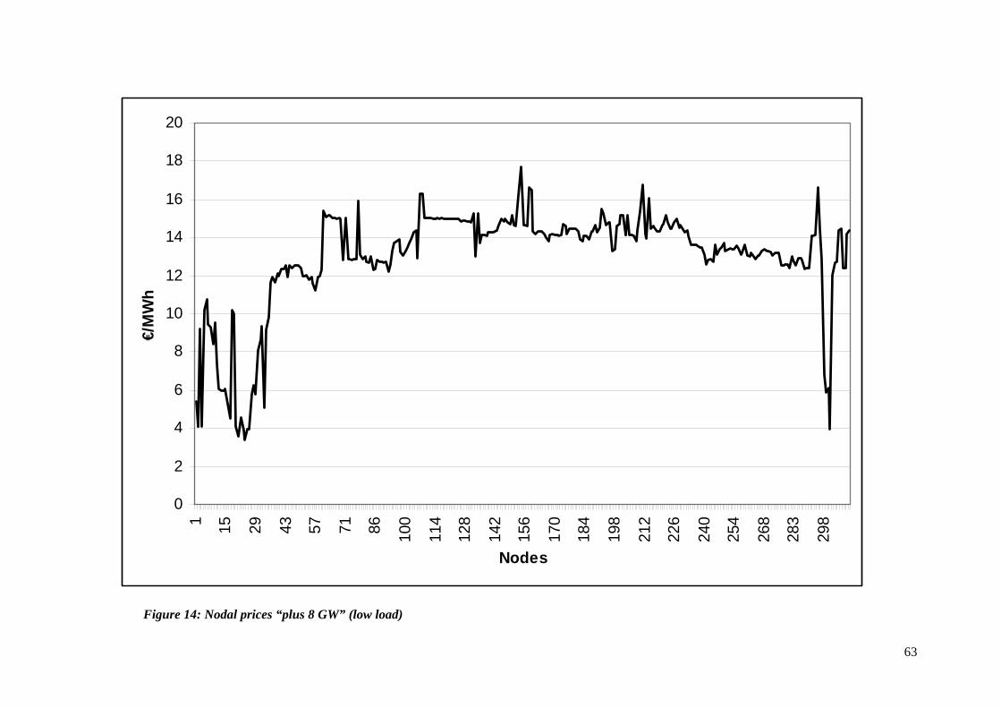
63

0

2

4

6

8

10

12

14

16

18

20

1 15 29 43 57 71 86 100

114

128

142

156

170

184

198

212

226

240

254

268

283

298

Nodes

€/M

Wh

Figure 14: Nodal prices “plus 8 GW” (low load)

64

Node Price Node Price Node Price Node Price Node Price Node Price Node Price

1 5.42 46 12.40 91 12.74 136 14.12 181 14.30 226 14.76 271 13.27

2 4.05 47 12.54 92 12.20 137 14.13 182 13.90 227 14.94 272 13.07

3 9.23 48 12.55 93 12.64 138 14.05 183 13.84 228 14.53 273 13.19

4 4.05 49 12.55 94 13.33 139 14.26 184 14.05 229 14.63 274 13.17

5 10.19 50 12.43 95 13.69 140 14.28 185 14.05 230 14.49 275 13.15

6 10.76 51 11.99 96 13.83 141 14.29 186 13.86 231 14.27 276 12.55

7 9.46 52 11.99 97 13.90 142 14.31 187 14.31 232 14.39 277 12.57

8 9.30 53 12.06 98 13.23 143 14.39 188 14.32 233 14.10 278 12.60

9 8.43 54 11.80 99 13.03 144 14.68 189 14.62 234 13.64 279 12.63

10 9.55 55 11.88 100 13.34 145 14.97 190 14.26 235 13.63 281 12.44

11 7.36 56 11.59 101 13.49 146 14.87 191 14.53 236 13.62 282 12.99

12 6.05 57 11.24 102 13.68 147 14.95 192 15.49 237 13.55 283 12.78

13 5.97 58 11.94 103 13.89 148 14.76 193 15.28 238 13.52 284 12.52

14 6.01 59 12.01 104 14.25 149 14.69 194 14.65 239 13.49 285 12.94

15 6.03 60 12.26 105 14.40 150 15.17 195 14.79 240 13.11 286 12.94

16 5.31 61 15.44 106 12.90 151 14.68 196 14.80 241 12.64 287 12.81

17 4.49 62 15.11 107 16.32 152 14.57 197 13.33 242 12.77 288 12.38

18 10.19 63 15.14 108 16.31 153 16.16 198 13.35 243 12.89 289 12.41

19 10.00 64 15.15 109 15.03 154 17.69 199 14.58 244 12.77 290 12.40

20 4.05 65 15.03 110 15.02 155 14.66 200 14.70 245 13.64 292 14.05

21 3.57 66 15.01 111 15.03 156 14.67 201 15.18 246 13.13 293 14.06

22 4.57 67 14.99 112 15.02 157 14.60 202 15.15 247 13.35 294 14.17

23 3.91 68 15.02 113 15.00 158 16.62 203 14.13 248 13.51 295 16.65

24 3.38 69 14.96 114 15.00 159 16.48 204 15.18 249 13.70 296 14.47

25 3.97 70 12.79 115 15.00 160 14.36 205 14.15 250 13.33 297 12.84

26 3.97 71 15.01 116 15.00 161 14.18 206 14.14 251 13.36 298 6.79

27 5.77 73 12.84 117 15.04 162 14.32 207 14.09 252 13.43 299 5.89

28 6.25 74 12.85 118 15.00 163 14.34 208 13.82 253 13.35 300 6.08

29 5.82 75 12.83 119 14.99 164 14.35 209 14.38 254 13.38 301 3.96

30 8.12 76 12.86 120 14.98 165 14.19 210 15.35 255 13.54 302 12.06

31 8.68 77 12.85 121 14.98 166 14.03 211 16.75 256 13.42 303 12.65

32 9.35 78 15.94 122 14.98 167 13.80 212 14.20 257 13.14 304 12.76

33 5.08 79 13.14 123 14.99 168 14.12 213 13.98 258 13.16 305 14.37

34 9.20 80 12.88 124 15.00 169 14.18 214 16.05 259 13.63 306 14.43

35 9.78 81 12.99 125 14.94 170 14.17 215 14.48 260 13.06 307 12.44

36 11.64 82 12.77 126 14.86 171 14.15 216 14.56 261 13.02 308 12.45

37 11.92 83 12.67 127 14.92 172 14.09 217 14.52 262 13.16 309 14.23

38 11.68 84 12.98 128 14.93 173 14.11 218 14.34 263 13.00 310 14.42

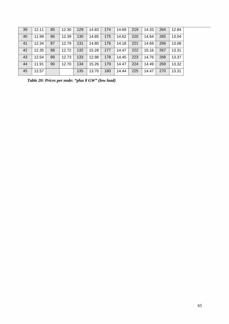
65

39 12.11 85 12.30 129 14.83 174 14.69 219 14.33 264 12.84 40 11.99 86 12.39 130 14.85 175 14.62 220 14.64 265 13.04 41 12.34 87 12.79 131 14.80 176 14.18 221 14.69 266 13.08 42 12.35 88 12.72 132 15.28 177 14.47 222 15.16 267 13.31 43 12.54 89 12.73 133 12.98 178 14.45 223 14.76 268 13.37 44 11.91 90 12.70 134 15.26 179 14.47 224 14.49 269 13.32 45 12.57 135 13.70 180 14.44 225 14.47 270 13.31

Table 20: Prices per node: “plus 8 GW” (low load)

66

0

5

10

15

20

25

30

35

40

45

1 15 29 43 57 71 86 100

114

128

142

156

170

184

198

212

226

240

254

268

283

298

Nodes

€/M

Wh

Figure 15: Nodal prices “plus 8 GW” (high load)

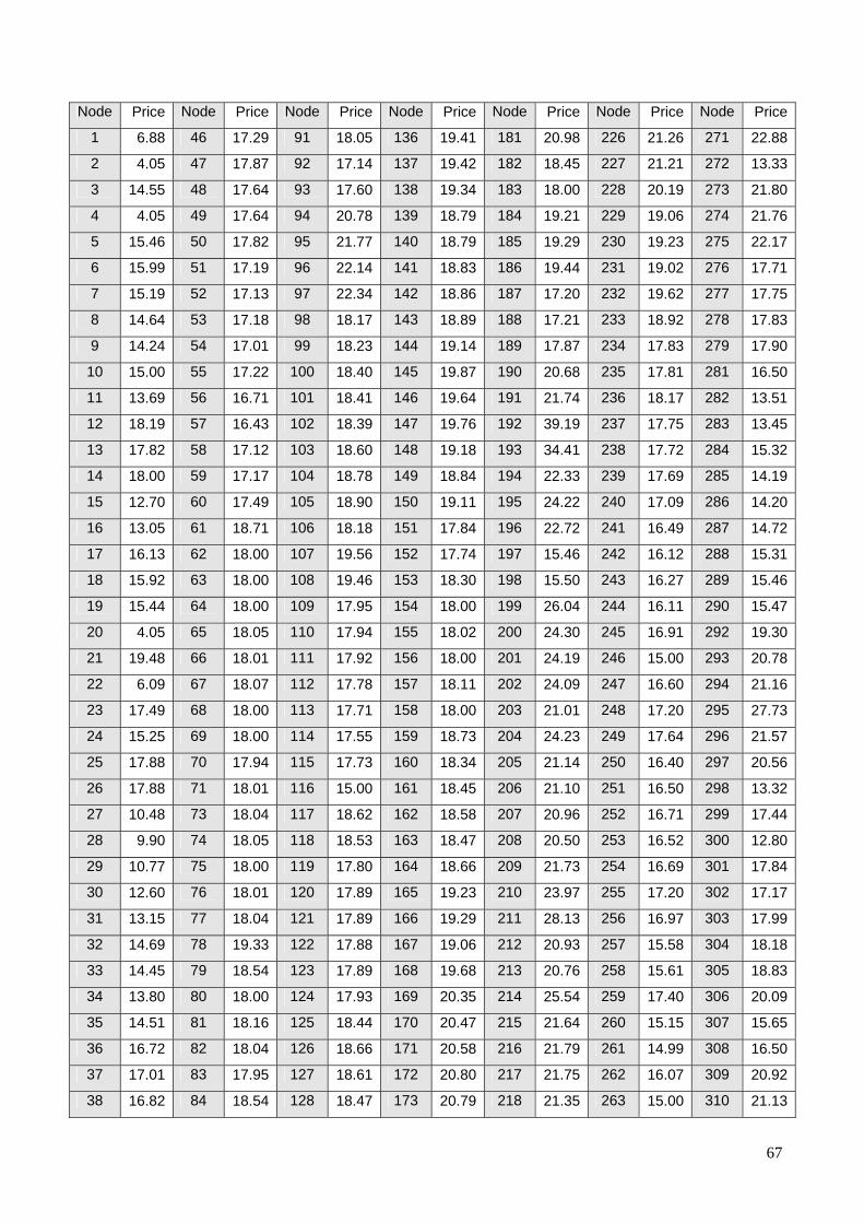
67

Node Price Node Price Node Price Node Price Node Price Node Price Node Price

1 6.88 46 17.29 91 18.05 136 19.41 181 20.98 226 21.26 271 22.88

2 4.05 47 17.87 92 17.14 137 19.42 182 18.45 227 21.21 272 13.33

3 14.55 48 17.64 93 17.60 138 19.34 183 18.00 228 20.19 273 21.80

4 4.05 49 17.64 94 20.78 139 18.79 184 19.21 229 19.06 274 21.76

5 15.46 50 17.82 95 21.77 140 18.79 185 19.29 230 19.23 275 22.17

6 15.99 51 17.19 96 22.14 141 18.83 186 19.44 231 19.02 276 17.71

7 15.19 52 17.13 97 22.34 142 18.86 187 17.20 232 19.62 277 17.75

8 14.64 53 17.18 98 18.17 143 18.89 188 17.21 233 18.92 278 17.83

9 14.24 54 17.01 99 18.23 144 19.14 189 17.87 234 17.83 279 17.90

10 15.00 55 17.22 100 18.40 145 19.87 190 20.68 235 17.81 281 16.50

11 13.69 56 16.71 101 18.41 146 19.64 191 21.74 236 18.17 282 13.51

12 18.19 57 16.43 102 18.39 147 19.76 192 39.19 237 17.75 283 13.45

13 17.82 58 17.12 103 18.60 148 19.18 193 34.41 238 17.72 284 15.32

14 18.00 59 17.17 104 18.78 149 18.84 194 22.33 239 17.69 285 14.19

15 12.70 60 17.49 105 18.90 150 19.11 195 24.22 240 17.09 286 14.20

16 13.05 61 18.71 106 18.18 151 17.84 196 22.72 241 16.49 287 14.72

17 16.13 62 18.00 107 19.56 152 17.74 197 15.46 242 16.12 288 15.31

18 15.92 63 18.00 108 19.46 153 18.30 198 15.50 243 16.27 289 15.46

19 15.44 64 18.00 109 17.95 154 18.00 199 26.04 244 16.11 290 15.47

20 4.05 65 18.05 110 17.94 155 18.02 200 24.30 245 16.91 292 19.30

21 19.48 66 18.01 111 17.92 156 18.00 201 24.19 246 15.00 293 20.78

22 6.09 67 18.07 112 17.78 157 18.11 202 24.09 247 16.60 294 21.16

23 17.49 68 18.00 113 17.71 158 18.00 203 21.01 248 17.20 295 27.73

24 15.25 69 18.00 114 17.55 159 18.73 204 24.23 249 17.64 296 21.57

25 17.88 70 17.94 115 17.73 160 18.34 205 21.14 250 16.40 297 20.56

26 17.88 71 18.01 116 15.00 161 18.45 206 21.10 251 16.50 298 13.32

27 10.48 73 18.04 117 18.62 162 18.58 207 20.96 252 16.71 299 17.44

28 9.90 74 18.05 118 18.53 163 18.47 208 20.50 253 16.52 300 12.80

29 10.77 75 18.00 119 17.80 164 18.66 209 21.73 254 16.69 301 17.84

30 12.60 76 18.01 120 17.89 165 19.23 210 23.97 255 17.20 302 17.17

31 13.15 77 18.04 121 17.89 166 19.29 211 28.13 256 16.97 303 17.99

32 14.69 78 19.33 122 17.88 167 19.06 212 20.93 257 15.58 304 18.18

33 14.45 79 18.54 123 17.89 168 19.68 213 20.76 258 15.61 305 18.83

34 13.80 80 18.00 124 17.93 169 20.35 214 25.54 259 17.40 306 20.09

35 14.51 81 18.16 125 18.44 170 20.47 215 21.64 260 15.15 307 15.65

36 16.72 82 18.04 126 18.66 171 20.58 216 21.79 261 14.99 308 16.50

37 17.01 83 17.95 127 18.61 172 20.80 217 21.75 262 16.07 309 20.92

38 16.82 84 18.54 128 18.47 173 20.79 218 21.35 263 15.00 310 21.13

68

39 17.20 85 17.41 129 18.63 174 24.27 219 21.33 264 16.10 40 17.40 86 17.54 130 18.89 175 24.06 220 21.48 265 14.43 41 18.00 87 18.05 131 17.84 176 20.89 221 21.40 266 13.17 42 17.98 88 18.04 132 20.15 177 21.25 222 22.69 267 24.91 43 18.54 89 18.02 133 18.21 178 21.21 223 21.53 268 24.60 44 16.96 90 17.96 134 18.47 179 21.24 224 20.82 269 24.35 45 18.04 135 18.93 180 21.14 225 20.46 270 23.77

Table 21: Prices per node: “plus 8 GW” (high load)

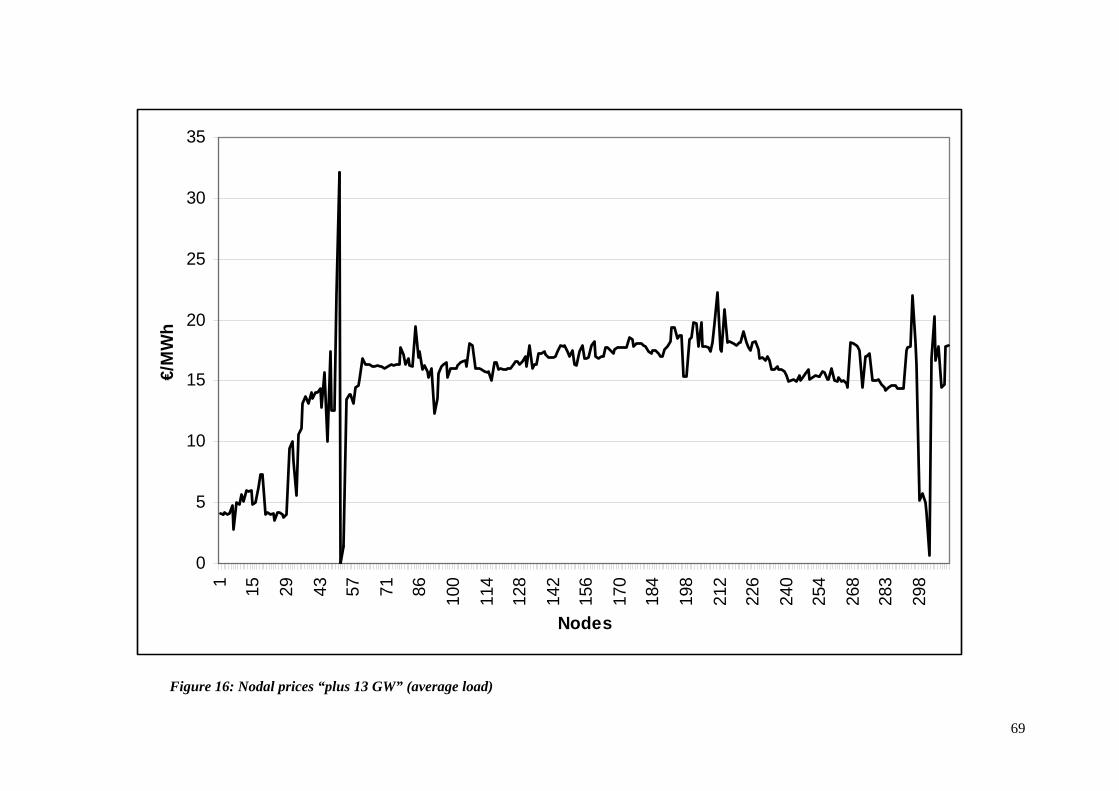
69

0

5

10

15

20

25

30

35

1 15 29 43 57 71 86 100

114

128

142

156

170

184

198

212

226

240

254

268

283

298

Nodes

€/M

Wh

Figure 16: Nodal prices “plus 13 GW” (average load)

70

Node Price Node Price Node Price Node Price Node Price Node Price Node Price

1 4.07 46 10.08 91 16.02 136 17.28 181 17.83 226 18.11 271 17.52

2 4.05 47 17.38 92 12.41 137 17.29 182 17.33 227 18.31 272 14.49

3 4.25 48 12.56 93 13.63 138 17.44 183 17.26 228 17.62 273 17.10

4 4.05 49 12.56 94 15.56 139 17.12 184 17.53 229 16.81 274 17.08

5 4.11 50 22.23 95 16.15 140 17.00 185 17.52 230 16.91 275 17.23

6 4.84 51 32.07 96 16.38 141 16.92 186 17.32 231 16.74 276 15.00

7 2.80 52 0.00 97 16.50 142 16.95 187 17.07 232 17.06 277 15.02

8 5.01 53 1.43 98 15.29 143 17.10 188 17.08 233 16.71 278 15.08

9 4.85 54 13.49 99 16.05 144 17.33 189 17.59 234 15.95 279 15.13

10 5.65 55 13.94 100 16.08 145 17.99 190 17.81 235 15.94 281 14.67

11 5.14 56 13.90 101 16.07 146 17.82 191 18.28 236 16.13 282 14.50

12 6.02 57 13.12 102 16.25 147 17.95 192 19.45 237 15.91 283 14.30

13 5.90 58 14.51 103 16.53 148 17.38 193 19.38 238 15.89 284 14.48

14 5.96 59 14.60 104 16.66 149 17.10 194 18.48 239 15.86 285 14.60

15 4.96 60 15.20 105 16.74 150 17.54 195 18.77 240 15.52 286 14.61

16 5.03 61 16.87 106 16.17 151 16.34 196 18.74 241 14.92 287 14.64

17 6.23 62 16.36 107 18.05 152 16.24 197 15.35 242 15.00 288 14.37

18 7.37 63 16.36 108 18.00 153 17.37 198 15.39 243 15.11 289 14.43

19 7.38 64 16.33 109 16.06 154 18.00 199 18.45 244 14.99 290 14.43

20 4.05 65 16.21 110 16.04 155 16.86 200 18.60 245 15.49 292 17.51

21 4.29 66 16.22 111 16.04 156 16.88 201 19.82 246 15.00 293 17.69

22 4.00 67 16.24 112 15.91 157 16.91 202 19.75 247 15.34 294 17.89

23 4.16 68 16.21 113 15.84 158 18.00 203 17.82 248 15.64 295 22.11

24 3.61 69 16.19 114 15.69 159 18.23 204 19.83 249 15.95 296 18.14

25 4.24 70 16.10 115 15.86 160 17.03 205 17.87 250 15.21 297 16.43

26 4.24 71 16.18 116 15.00 161 16.86 206 17.84 251 15.30 298 5.26

27 3.98 73 16.29 117 16.53 162 17.02 207 17.75 252 15.47 299 5.78

28 3.76 74 16.33 118 16.48 163 17.03 208 17.40 253 15.33 300 5.00

29 4.05 75 16.23 119 15.92 164 17.71 209 18.20 254 15.43 301 4.23

30 9.44 76 16.40 120 16.00 165 17.68 210 19.68 255 15.85 302 0.72

31 10.00 77 16.36 121 16.00 166 17.51 211 22.34 256 15.69 303 16.81

32 8.41 78 17.68 122 15.99 167 17.26 212 17.63 257 15.11 304 20.31

33 5.55 79 17.14 123 16.00 168 17.58 213 17.44 258 15.13 305 16.69

34 10.56 80 16.42 124 16.03 169 17.76 214 20.81 259 16.00 306 17.85

35 11.17 81 16.86 125 16.42 170 17.77 215 18.15 260 15.00 307 14.50

36 13.12 82 16.30 126 16.56 171 17.77 216 18.24 261 14.91 308 14.67

37 13.70 83 16.19 127 16.64 172 17.72 217 18.22 262 15.24 309 17.81

38 13.18 84 19.52 128 16.44 173 17.74 218 18.02 263 14.90 310 17.98

71

39 14.10 85 16.97 129 16.57 174 18.58 219 18.00 264 15.02 40 13.61 86 17.43 130 17.02 175 18.45 220 18.22 265 14.77 41 14.06 87 15.90 131 16.12 176 17.79 221 18.22 266 14.46 42 14.05 88 16.32 132 17.90 177 18.06 222 19.04 267 18.15 43 14.40 89 15.87 133 16.10 178 18.03 223 18.18 268 18.09 44 12.84 90 15.29 134 16.40 179 18.05 224 17.71 269 18.00 45 15.68 135 16.42 180 18.00 225 17.52 270 17.82

Table 22: Prices per node: “plus 13 GW” (average load)

72

0

2

4

6

8

10

12

14

16

18

20

1 15 29 43 57 71 86 100

114

128

142

156

170

184

198

212

226

240

254

268

283

298

Nodes

€/M

Wh

Figure 17: Nodal prices “plus 13 GW” (low load)

73

Node Price Node Price Node Price Node Price Node Price Node Price Node Price

1 4.17 46 8.40 91 9.56 136 13.64 181 13.89 226 14.35 271 12.25

2 4.05 47 9.21 92 9.85 137 13.65 182 13.49 227 14.51 272 12.13

3 4.64 48 8.91 93 10.54 138 13.63 183 13.43 228 14.12 273 12.17

4 4.05 49 8.91 94 11.25 139 13.67 184 13.64 229 14.33 274 12.16

5 3.89 50 9.01 95 11.56 140 13.57 185 13.64 230 14.14 275 12.14

6 2.34 51 8.27 96 11.67 141 13.51 186 13.46 231 13.90 276 11.42

7 5.46 52 7.62 97 11.73 142 13.53 187 14.01 232 14.01 277 11.43

8 5.02 53 6.65 98 11.47 143 13.78 188 14.02 233 13.65 278 11.46

9 4.88 54 8.58 99 10.61 144 14.16 189 14.31 234 13.21 279 11.49

10 5.36 55 9.10 100 11.52 145 14.48 190 13.85 235 13.21 281 11.37

11 4.94 56 10.00 101 11.91 146 14.38 191 14.11 236 12.58 282 12.05

12 5.41 57 10.48 102 12.46 147 14.46 192 15.13 237 12.85 283 11.85

13 5.34 58 9.89 103 12.82 148 14.27 193 14.90 238 12.73 284 11.50

14 5.38 59 9.90 104 13.34 149 14.32 194 14.23 239 12.70 285 11.97

15 4.59 60 9.91 105 13.57 150 14.80 195 14.38 240 12.28 286 11.97

16 4.51 61 16.08 106 10.32 151 14.47 196 14.37 241 11.71 287 11.83

17 5.51 62 15.75 107 15.92 152 14.37 197 13.33 242 11.91 288 11.37

18 6.26 63 15.70 108 15.91 153 15.83 198 13.34 243 12.05 289 11.39

19 6.27 64 15.63 109 15.24 154 17.34 199 14.18 244 11.91 290 11.38

20 4.05 65 15.70 110 15.15 155 14.38 200 14.29 245 12.93 292 13.63

21 4.41 66 15.81 111 15.21 156 14.39 201 14.75 246 12.39 293 13.66

22 3.86 67 15.95 112 15.08 157 14.29 202 14.72 247 12.65 294 13.76

23 4.17 68 15.76 113 15.00 158 16.22 203 13.73 248 12.96 295 16.18

24 3.60 69 15.91 114 15.00 159 16.07 204 14.75 249 13.14 296 14.07

25 4.22 70 9.33 115 15.01 160 13.98 205 13.75 250 12.74 297 11.91

26 4.22 71 15.67 116 15.00 161 13.75 206 13.74 251 12.75 298 4.96

27 3.57 73 9.52 117 14.85 162 13.92 207 13.69 252 12.80 299 5.26

28 3.28 74 9.57 118 14.81 163 13.95 208 13.42 253 12.72 300 4.63

29 3.60 75 9.46 119 14.95 164 13.95 209 13.98 254 12.74 301 4.22

30 8.31 76 9.61 120 14.89 165 13.79 210 14.92 255 12.92 302 7.25

31 8.60 77 9.62 121 14.89 166 13.63 211 16.29 256 12.81 303 9.40

32 7.25 78 15.55 122 14.90 167 13.40 212 13.82 257 12.40 304 9.67

33 4.92 79 10.00 123 14.91 168 13.69 213 13.59 258 12.41 305 13.54

34 8.86 80 9.62 124 14.91 169 13.75 214 15.60 259 13.01 306 14.01

35 9.14 81 9.88 125 14.75 170 13.75 215 14.07 260 12.26 307 11.42

36 10.02 82 9.79 126 14.64 171 13.74 216 14.15 261 12.20 308 11.38

37 10.45 83 9.90 127 14.68 172 13.68 217 14.11 262 12.39 309 13.81

38 10.06 84 9.85 128 14.70 173 13.70 218 13.94 263 12.16 310 14.00

74

39 10.74 85 9.71 129 14.45 174 14.28 219 13.93 264 11.98 40 10.10 86 9.82 130 14.54 175 14.21 220 14.22 265 12.17 41 10.12 87 9.86 131 14.65 176 13.77 221 14.27 266 12.15 42 10.01 88 9.57 132 14.84 177 14.05 222 14.73 267 12.32 43 10.29 89 9.57 133 10.50 178 14.04 223 14.38 268 12.37 44 9.96 90 9.45 134 15.17 179 14.05 224 14.11 269 12.32 45 9.79 135 12.09 180 14.02 225 14.10 270 12.30

Table 23: Prices per node: “plus 13 GW” (low load)

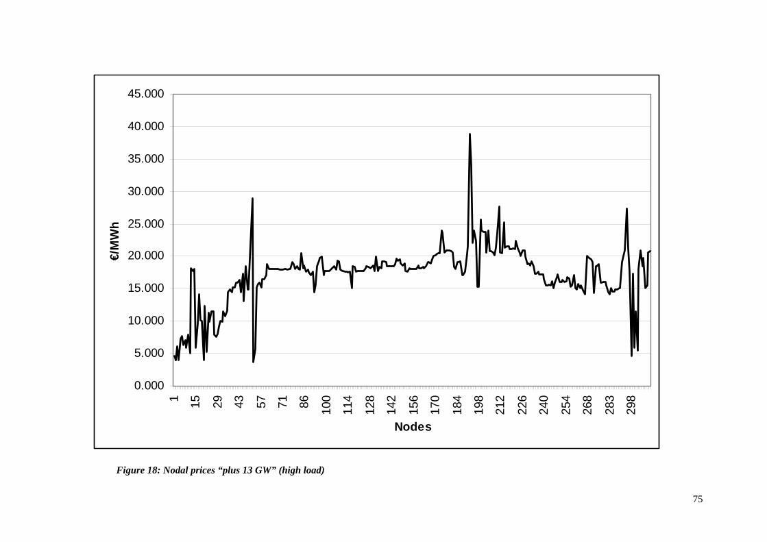
75

0.000

5.000

10.000

15.000

20.000

25.000

30.000

35.000

40.000

45.000

1 15 29 43 57 71 86 100

114

128

142

156

170

184

198

212

226

240

254

268

283

298

Nodes

€/M

Wh

Figure 18: Nodal prices “plus 13 GW” (high load)

76

Node Price Node Price Node Price Node Price Node Price Node Price Node Price

1 4.60 46 13.00 91 17.64 136 19.13 181 20.65 226 20.92 271 19.01

2 4.05 47 18.46 92 14.46 137 19.14 182 18.39 227 20.88 272 14.30

3 6.21 48 14.96 93 15.58 138 19.12 183 18.00 228 19.89 273 18.44

4 4.05 49 14.96 94 18.47 139 18.46 184 19.03 229 18.78 274 18.45

5 7.34 50 21.99 95 19.37 140 18.43 185 19.11 230 18.91 275 18.82

6 7.77 51 28.94 96 19.71 141 18.44 186 19.20 231 18.66 276 15.93

7 6.24 52 3.73 97 19.89 142 18.47 187 17.00 232 19.26 277 15.97

8 7.00 53 5.67 98 17.08 143 18.56 188 17.01 233 18.44 278 16.04

9 5.94 54 15.20 99 17.77 144 18.84 189 17.67 234 17.37 279 16.10

10 7.86 55 15.76 100 17.82 145 19.58 190 20.38 235 17.36 281 15.42

11 5.08 56 15.87 101 17.77 146 19.35 191 21.43 236 17.62 282 14.41

12 18.19 57 15.26 102 17.83 147 19.47 192 38.79 237 17.24 283 14.24

13 17.79 58 16.46 103 18.09 148 18.89 193 34.03 238 17.19 284 15.00

14 18.00 59 16.48 104 18.35 149 18.61 194 22.00 239 17.17 285 14.67

15 5.89 60 17.03 105 18.49 150 18.93 195 23.88 240 16.45 286 14.67

16 9.57 61 18.71 106 17.90 151 17.78 196 22.40 241 15.49 287 14.91

17 14.25 62 18.00 107 19.30 152 17.67 197 15.28 242 15.42 288 14.95

18 10.17 63 18.00 108 19.20 153 18.23 198 15.32 243 15.57 289 15.02

19 10.00 64 18.00 109 17.85 154 18.00 199 25.69 244 15.42 290 15.03

20 4.05 65 18.01 110 17.83 155 18.00 200 23.95 245 16.20 292 19.10

21 12.28 66 18.00 111 17.82 156 18.00 201 23.85 246 15.00 293 20.48

22 5.25 67 18.01 112 17.67 157 18.05 202 23.76 247 15.90 294 20.86

23 11.27 68 18.00 113 17.60 158 18.00 203 20.71 248 16.72 295 27.33

24 9.83 69 17.94 114 17.43 159 18.69 204 23.89 249 17.15 296 21.25

25 11.53 70 17.84 115 17.62 160 18.13 205 20.84 250 15.98 297 17.70

26 11.53 71 17.96 116 15.00 161 18.20 206 20.80 251 16.08 298 4.60

27 7.86 73 18.01 117 18.42 162 18.35 207 20.66 252 16.28 299 17.37

28 7.56 74 18.03 118 18.34 163 18.25 208 20.21 253 16.09 300 5.93

29 8.08 75 17.96 119 17.67 164 18.43 209 21.42 254 16.26 301 11.51

30 9.21 76 18.03 120 17.75 165 19.01 210 23.62 255 16.81 302 5.38

31 10.00 77 18.03 121 17.75 166 19.07 211 27.73 256 16.59 303 18.00

32 9.92 78 19.07 122 17.74 167 18.88 212 20.60 257 15.39 304 20.92

33 11.48 79 18.82 123 17.75 168 19.46 213 20.44 258 15.42 305 18.42

34 10.78 80 18.00 124 17.80 169 20.09 214 25.17 259 17.01 306 19.80

35 11.65 81 18.43 125 18.24 170 20.20 215 21.32 260 15.05 307 15.11

36 14.41 82 18.00 126 18.43 171 20.30 216 21.47 261 14.97 308 15.43

37 14.86 83 17.89 127 18.40 172 20.50 217 21.43 262 15.74 309 20.61

38 14.49 84 20.54 128 18.26 173 20.50 218 21.04 263 15.00 310 20.80

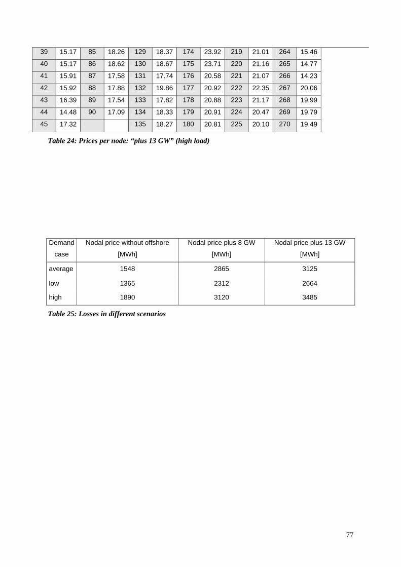
77

39 15.17 85 18.26 129 18.37 174 23.92 219 21.01 264 15.46 40 15.17 86 18.62 130 18.67 175 23.71 220 21.16 265 14.77 41 15.91 87 17.58 131 17.74 176 20.58 221 21.07 266 14.23 42 15.92 88 17.88 132 19.86 177 20.92 222 22.35 267 20.06 43 16.39 89 17.54 133 17.82 178 20.88 223 21.17 268 19.99 44 14.48 90 17.09 134 18.33 179 20.91 224 20.47 269 19.79 45 17.32 135 18.27 180 20.81 225 20.10 270 19.49

Table 24: Prices per node: “plus 13 GW” (high load)

Demand

case

Nodal price without offshore

[MWh]

Nodal price plus 8 GW

[MWh]

Nodal price plus 13 GW

[MWh]

average 1548 2865 3125

low 1365 2312 2664

high 1890 3120 3485

Table 25: Losses in different scenarios

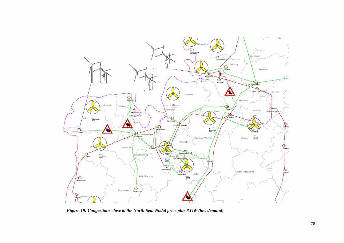
78

Figure 19: Congestions close to the North Sea: Nodal price plus 8 GW (low demand)

79

Figure 20: Congestions close the North Sea: Nodal price plus 8 GW (high demand)

80

Figure 21: Congestions close to the North Sea: Nodal price plus 13 GW (low demand)

81

Figure 22: Congestions close to the North Sea: Nodal price plus 13 GW (high demand)