Nodal curves and polarizations with good properties

Revista Matemática Complutensehttps://doi.org/10.1007/s13163-021-00404-z

Nodal curves and polarizations with good properties

Sonia Brivio1 · Filippo F. Favale1

Received: 11 November 2020 / Accepted: 21 July 2021© The Author(s) 2021

AbstractIn this paper we deal with polarizations on a nodal curve C with smooth components.Our aim is to study and characterize a class of polarizations, which we call “good”,for which depth one sheaves on C reflect some properties that hold for vector bundleson smooth curves. We will concentrate, in particular, on the relation between the w-stability of OC and the goodness of w. We prove that these two concepts agree whenC is of compact type and we conjecture that the same should hold for all nodal curves.

Keyword Polarizations, Stability, Nodal curves, Moduli spaces

Mathematics Subject Classification Primary: 14H60; Secondary: 14F06 · 14D20

Introduction

LetC be a projective curve over the complexfield.Oneof themost interesting problemsinAlgebraic Geometry is the construction ofmoduli spaces parametrizing line bundlesor in general vector bundles on C . These moduli spaces have been studied first byMumford [22] and Le Potier [21] in the smooth case. These spaces are interesting bythemselves as higher dimensional varieties but also for important related constructions:just tomention some, one can consider higher-rankBrill-Noether theory,Theta divisorsand Theta functions and the moduli spaces of coherent systems. For surveys on thesetopics see, for example [3,6,7]; for some results by the authors see [5,8,11–14]. Whenthe curve is singular, these spaces are not in general complete. It is natural to study theirpossible compactifications and this has driven the attention of many authors since the

Sonia Brivio and Filippo F. Favale have partially supported by INdAM - GNSAGA.

B Filippo F. [email protected]

Sonia [email protected]

1 Dipartimento di Matematica e Applicazioni, Università degli Studi di Milano-Bicocca, Via RobertoCozzi, 55, I-20125 Milano, Italy

123

S. Brivio, F. F. Favale

’60s, who addressed the problem with different approaches (see, for instance, [4,18–20,23,24]).WhenC is a reducible nodal curve, that is it has only ordinary double points,we have more explicit results. In several of the constructions mentioned above, theobjects of these compact moduli spaces are equivalence classes of depth one sheaves(i.e. torsion free) on the curve that are semistable with respect to a polarization (see[25,26]).

A polarization w on C is given by rational weights on each irreducible componentofC adding up to 1 or, equivalently, by an ample line bundle L onC (see [20,24]). Oncea polarization on the curve is fixed, the notions of degree and rank can be generalizedto the notions of w-degree and w-rank which are also defined for depth one sheaves.With these data Seshadri introduced the notion of w-stability (or w-semistability) fordepth one sheaves allowing the construction of moduli spaces of such objects.

In this paper we are interested in studying polarizations on nodal reducible curveshaving nice properties, i.e. which allow us to generalize to nodal curves some naturalproperties of vector bundles on smooth curves and to simplify the study of stabilityof vector bundles and coherent systems on nodal reducible curves. As motivation,consider the following facts. On a smooth curve C , the sheaf OC is stable (as all linebundles) and any globally generated vector bundle has non-negative degree. This isnot true anymore on reducible nodal curves. Moreover, in order to construct vectorbundles on a reducible nodal curve, one can glue vector bundles on its components.In general, though, it is not true that glueing stable vector bundles yields a w-stablesheaf: additional conditions on the polarization and on the degree of the restrictionsare needed (see [9,10,27]).

This motivates our definition of a good polarization. Let C be a nodal curve withγ smooth irreducible components. For any depth one sheaf E on C , we denote by Ei

the restriction (modulo torsion) of E to the component Ci . Note that if E is locallyfree, then the degree of E is actually the sum of the degrees of its restrictions Ei , butthis is not true in general. We will say that w is a good polarization if for any depthone sheaf E the difference �w(E) of the w-degree of E and the sum of degrees ofits restrictions Ei is non negative and it is zero if and only if E is locally free (seeDefinition 2.6). As anticipated, the first result of this paper is the following:

Theorem (Theorem 2.9) Let C be a nodal curve and let w be a good polarization onit. Let E be a depth one sheaf on C. Then we have the following properties:

(a) Assume that E is locally free and, for i = 1, . . . , γ , Ei is stable with deg(Ei ) = 0.Then E is w-stable.

(b) If E is globally generated, then degw(E) ≥ 0.

(c) If E is w-semistable and degw(E) > 0, then h0(E∗) = 0.

In particular, if E = OC or, more generally, if E is a line bundle whose restrictionshave degree 0, then E is w-stable.

Wewill show that goodpolarizations exist on any stable nodal curvewith pa(C) ≥ 2(see Proposition 2.8 and Corollary 3.15). For nodal curves with pa(C) ≤ 1we are ableto characterize exactly which curves admit a good polarization (see Corollary 3.11).

The second result of this paper provides sufficient conditions in order to obtain agood polarization on a nodal curve. The method relies on the choice of particular paths

123

Nodal curves and polarizations with good properties

on the dual graph �C of C which yields a finite collection of subcurves A j of C . Thisallows us to get a rather technical description of �w(E), for any depth one sheaf E onC , and to obtain the mentioned sufficient conditions. These are stated in Theorem 3.9.More precisely, consider, for each non-empty subcurve A j , the condition

(��)A j : 1

2(δA j − 1) < �w(OA j ) <

1

2(δA j + 1)

where δA j is the number of the nodes of C lying on A j which are not nodes for thesubcurve A j (see Sect. 1 for details). Then we have the following:

Theorem (Theorem 3.9) Let (C, w) be a polarized nodal curve. If conditions (��)A j

hold for all non empty A j , then w is a good polarization.

Motivated by many examples (some of them have been reported in Sect. 4), wemake this conjecture:

Conjecture (Conjecture 3.13) Let (C, w) be a polarized nodal curve. Then OC isw-stable if and only if w is a good polarization.

In the third result of this paper we prove that this conjecture holds for curves ofcompact type:

Theorem (Theorem 3.10) Let (C, w) be a polarized nodal curve of compact type.Then OC is w-stable if and only if w is a good polarization.

The idea is to prove that conditions (��)A j are always implied by stability of OC

in the case of curves of compact type.Finally, we wonder how being a good polarization reflects on the line bundle induc-

ing the polarization. This turns out to be related to the notion of balanced line bundles,as defined in [15]. Balanced line bundles are important tools when one has to dealwith reducible nodal curves. For example, for such line bundles, a generalization ofClifford’s Theorem holds. Our results can be summarized as (see Corollary 2.19 andCorollary 3.12):

Theorem Let C be a stable nodal curve with pa(C) ≥ 2. Let L be a line bundle ofdegree pa(C) − 1 and w be the polarization induced by L. Then:

(1) L is strictly balanced if and only if OC is w-stable;(2) if C is of compact type, then L is strictly balanced if and only if w is good.

1 Notations and preliminary results on nodal curves

In this section we will introduce notations and we recall useful facts about nodalcurves, their subcurves and polarizations.

Let C be a connected reduced nodal curve over the complex field (i.e. having onlyordinary double points as singularities).Wewill denote by γ the number of irreduciblecomponents and by δ the number of nodes of C . We will assume that each irreducible

123

S. Brivio, F. F. Favale

component Ci is a smooth curve of genus gi . For the theory of nodal curves see [2,Ch X]. We will denote by

ν : Cν =⊔γ

i=1Ci → C

the normalization map. If p ∈ C is a node, we will denote by qp,i1 and qp,i2 the branchpoints over the node p, with qp,ik ∈ Cik . From the exact sequence:

0 → OC → ν∗ν∗(OC ) →⊕

p∈Sing(C)

Cp → 0,

we deduce that χ(OC ) = ∑γ

i=1 χ(OCi ) − δ, and we obtain the arithmetic genus ofC :

pa(C) =γ∑

i=1

gi + δ − γ + 1. (1.1)

The dual graph of C is the graph �C whose vertices are identified with the irreduciblecomponents of C and whose edges are identified with the nodes of C . An edge joinstwo vertices if the corresponding node is in the intersection of the correspondingirreducible components. So, �C has δ edges and γ vertices, moreover it is connectedsince C is connected. Its first Betti number is b1(�C ) = δ − γ + 1. We recall that aconnected nodal curve is said to be of compact type if every irreducible componentof C is smooth and its dual graph is a tree. For a curve of compact type we haveδ −γ +1 = 0 and the pull-back ν∗ of the normalization map induces an isomorphismPic(C) � ⊕γ

i=1 Pic(Ci ) between the Picard groups.Let B be a proper subcurve of C , the complementary curve of B is defined as the

closure of C \ B and it is denoted by Bc. We will denote by �B the Weil divisor�B = B · Bc = ∑

p∈B∩Bc p, we will denote its degree by δB so δB = #B ∩ Bc. Inparticular, when Ci is a component of C , �Ci is given by the nodes on Ci . To simplifynotations we set �Ci = �i and δi = #�i .

As the only singularities ofC are nodes,C can be embedded in a smooth projectivesurface, see [1]. This gives, for any proper subcurve B ofC , the following fundamentalexact sequence

0 → OBc (−�B) → OC → OB → 0, (1.2)

from which we deduce

pa(C) = pa(B) + pa(Bc) + δB − 1. (1.3)

We recall that a connected nodal curve C of arithmetic genus pa(C) ≥ 2 is calledstable if each smooth rational component E of C meets Ec in at least three points, i.e.δE ≥ 3. A curve is stable if and only if ωC is ample. The curve C is called semistableif δE ≥ 2. If C is semistable, a rational component E with δE = 2 is said to be an

123

Nodal curves and polarizations with good properties

exceptional component. Finally, C is called quasistable if it is semistable and if anytwo exceptional components do not intersect each other. Good references for thesetopics are [15,16].

Let L be a line bundle on C . For all i = 1, . . . , γ , let Li denote the restrictionof L to the component Ci . It is a line bundle on Ci with deg(Li ) = di . We will call(d1, . . . , dγ ) the multidegree of L . Then the degree of L is deg(L) = ∑γ

i=1 di . Wehave an exact sequence

0 → L → ν∗ν∗L →⊕

p∈Sing(C)

Cp → 0,

from which we deduce χ(L) = ∑γ

i=1 χ(Li ) − δ. In complete analogy with thesmooth case, Riemann-Roch’s Theorem holds for any line bundle L on C : χ(L) =deg(L)+1− pa(C). We recall that L is ample if and only if di > 0 for all i = 1, . . . γ .We will denote by Pic0(C) ⊂ Pic(C) the variety parametrizing the isomorphismclasses of line bundles on C having multidegree (0, . . . , 0).

There exists on C a dualizing sheaf ωC , which is invertible. For simplicity, if L is aline bundle on C and B is a subcurve of C , we will denote by degB(L) = degB(L|B)

the degree of L|B as line bundle on B. Then, we haveωC |B = ωB(B ·Bc), fromwhichwe obtain that the degree of ωC |B is degB(ωC |B) = 2pa(B) − 2 + δB . In particular,we have deg(ωC ) = 2pa(C) − 2.

A central object in this paper will be the notion of polarization. One can refer to[23,24] for details about polarizations and their role in studying stability of depth onesheaves on reducible nodal curves.

Definition 1.1 A polarization on the curve C is a vector w = (w1, . . . , wγ ) ∈ Qγ

such that

0 < wi < 1γ∑

i=1

wi = 1. (1.4)

We will say that the pair (C, w) is a polarized curve.

Remark 1.2 Let L be an ample line bundle on C , with deg(L) = d = ∑γ

i=1 di . Wecan associate to L a polarization wL on C by setting wL = 1

d (d1, . . . , dγ ). We willcallwL the polarization induced by L . Note that for any polarizationw there exists aline bundle L which induces w. Such a line bundle is not unique: many modificationsof L (for instance, one can consider a multiple of L), lead to the same polarization.

We recall that a depth one sheaf on a curve is a coherent sheaf E withdim Supp(F) = 1 for any subsheaf F of E . On a nodal curve this is equivalentto saying that E is torsion free. If E is a depth one sheaf on C and B is any propersubcurve of C , we denote by E |B the restriction of E to B and by EB the restrictionE |B modulo torsion. Then EB is a depth one sheaf on B. If Ci is an irreducible com-ponent of C we define Ei to be ECi . We denote by di the degree of Ei and ri the rankof Ei .

123

S. Brivio, F. F. Favale

Ifw is a polarization onC , we define thew-rank and thew-degree of E as rkw(E) =∑ri=1 riwi and degw(E) = χ(E) − rkw(E)χ(OC ) respectively.

Definition 1.3 Let w be a polarization on C and let E be a depth one sheaf on C . Thew-slope of E is defined as

μw(E) = χ(E)

rkw(E)= degw(E)

rkw(E)+ χ(OC ).

E is said to be w-semistable if for any proper subsheaf F of E we have μw(F) ≤μw(E), i.e. if

degw(F)

rkw(F)≤ degw(E)

rkw(E).

E is said to be w-stable if the above inequality is strict.

We stress that in the case of depth one sheaves having rank 1 on each irreduciblecomponent ofC ,manydifferent notions of semistability have been introduced.One cansee for instance [17,23], for two different approaches which give equivalent stabilityconditions. In particular, we recall the following characterization of w-semistability,see [23].

Proposition 1.4 Let (C, w) be a polarized curve and let L be a depth one sheaf withri = 1 for all i . Then L is w-semistable if and only if for any proper subcurve B of C

degw(LB) ≥ degw(L)rkw(LB).

It is w-stable if and only if the inequality is strict.

2 Polarizations with nice properties

From now on we will assume that C is a reducible nodal curve.

2.1 The function1w and its properties

Definition 2.1 Let w be a polarization on C . Let E be a depth one sheaf on C and letEi be the restricion of E to Ci modulo torsion. We define �w(E) as

�w(E) = degw(E) −γ∑

i=1

deg(Ei ).

Note that if pa(C) = 1, then �w(E) = χ(E) − ∑γ

i=1 deg(Ei ), so it does notdepend on the chosen polarization.

123

Nodal curves and polarizations with good properties

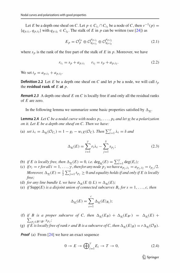
Let E be a depth one sheaf on C . Let p ∈ Ci1 ∩Ci2 be a node of C , then ν−1(p) ={qp,i1 , qp,i2} with qp,ik ∈ Cik . The stalk of E in p can be written (see [24]) as

Ep = Ospp ⊕ Oap,i1

qp,i1⊕ Oap,i2

qp,i2(2.1)

where sp is the rank of the free part of the stalk of E in p. Moreover, we have

ri1 = sp + ap,i1 ri2 = sp + ap,i2 . (2.2)

We set tp = ap,i1 + ap,i2 .

Definition 2.2 Let E be a depth one sheaf on C and let p be a node, we will call tpthe residual rank of E at p.

Remark 2.3 A depth one sheaf E on C is locally free if and only all the residual ranksof E are zero.

In the following lemma we summarize some basic properties satisfied by �w.

Lemma 2.4 Let C be a nodal curve with nodes p1, . . . , pδ and let w be a polarizationon it. Let E be a depth one sheaf on C. Then we have:

(a) set λi = �w(OCi ) = 1 − gi − wiχ(OC ). Then∑γ

i=1 λi = δ and

�w(E) =γ∑

i=1

riλi −δ∑

j=1

sp j ; (2.3)

(b) if E is locally free, then �w(E) = 0, i.e. degw(E) = ∑γ

i=1 deg(Ei );(c) if ri = r for all i = 1, . . . , γ , then for any node p j wehaveap j ,i1 = ap j ,i2 = tp j /2.

Moreover,�w(E) = 12

∑δj=1 tp j ≥ 0 and equality holds if and only if E is locally

free;(d) for any line bundle L we have �w(E ⊗ L) = �w(E);(e) if Supp(E) is a disjoint union of connected subcurves Bs for s = 1, . . . , c, then

�w(E) =c∑

s=1

�w(E |Bs );

(f) if B is a proper subcurve of C, then �w(EB) + �w(EBc ) = �w(E) +∑p j∈B∩Bc sp j ;

(g) if E is locally free of rank r and B is a subcurve of C, then�w(E |B) = r�w(OB).

Proof (a) From [24] we have an exact sequence

0 → E →⊕γ

i=1Ei → T → 0, (2.4)

123

S. Brivio, F. F. Favale

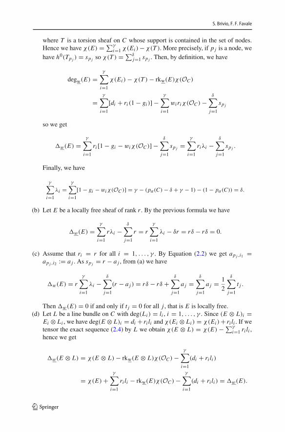
where T is a torsion sheaf on C whose support is contained in the set of nodes.Hence we have χ(E) = ∑γ

i=1 χ(Ei ) − χ(T ). More precisely, if p j is a node, wehave h0(Tp j ) = sp j so χ(T ) = ∑δ

j=1 sp j . Then, by definition, we have

degw(E) =γ∑

i=1

χ(Ei ) − χ(T ) − rkw(E)χ(OC )

=γ∑

i=1

[di + ri (1 − gi )] −γ∑

i=1

wi riχ(OC ) −δ∑

j=1

sp j

so we get

�w(E) =γ∑

i=1

ri [1 − gi − wiχ(OC )] −δ∑

j=1

sp j =γ∑

i=1

riλi −δ∑

j=1

sp j .

Finally, we have

γ∑

i=1

λi =γ∑

i=1

[1 − gi − wiχ(OC )] = γ − (pa(C) − δ + γ − 1) − (1 − pa(C)) = δ.

(b) Let E be a locally free sheaf of rank r . By the previous formula we have

�w(E) =γ∑

i=1

rλi −δ∑

j=1

r = rγ∑

i=1

λi − δr = rδ − rδ = 0.

(c) Assume that ri = r for all i = 1, . . . , γ . By Equation (2.2) we get ap j ,i1 =ap j ,i2 := a j . As sp j = r − a j , from (a) we have

�w(E) = rγ∑

i=1

λi −δ∑

j=1

(r − a j ) = rδ − rδ +δ∑

j=1

a j =δ∑

j=1

a j = 1

2

δ∑

j=1

t j .

Then �w(E) = 0 if and only if t j = 0 for all j , that is E is locally free.(d) Let L be a line bundle on C with deg(Li ) = li , i = 1, . . . , γ . Since (E ⊗ L)i =

Ei ⊗ Li , we have deg(E ⊗ L)i = di + ri li and χ(Ei ⊗ Li ) = χ(Ei ) + ri li . If wetensor the exact sequence (2.4) by L we obtain χ(E ⊗ L) = χ(E) − ∑γ

i=1 ri li ,hence we get

�w(E ⊗ L) = χ(E ⊗ L) − rkw(E ⊗ L)χ(OC ) −γ∑

i=1

(di + ri li )

= χ(E) +γ∑

i=1

ri li − rkw(E)χ(OC ) −γ∑

i=1

(di + ri li ) = �w(E).

123

Nodal curves and polarizations with good properties

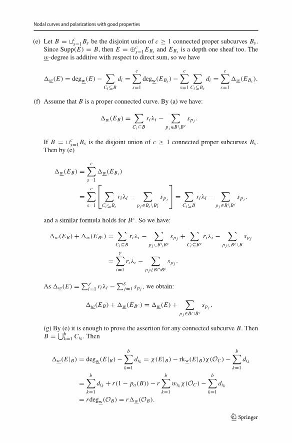
(e) Let B = �cs=1Bs be the disjoint union of c ≥ 1 connected proper subcurves Bs .

Since Supp(E) = B, then E = ⊕cs=1EBs and EBs is a depth one sheaf too. The

w-degree is additive with respect to direct sum, so we have

�w(E) = degw(E) −∑

Ci⊆B

di =c∑

s=1

degw(EBs ) −c∑

s=1

∑

Ci⊆Bs

di =c∑

s=1

�w(EBs ).

(f) Assume that B is a proper connected curve. By (a) we have:

�w(EB) =∑

Ci⊆B

riλi −∑

p j∈B\Bc

sp j .

If B = �cs=1Bs is the disjoint union of c ≥ 1 connected proper subcurves Bs .

Then by (e)

�w(EB) =c∑

s=1

�w(EBs )

=c∑

s=1

⎡

⎣∑

Ci⊆Bs

riλi −∑

p j∈Bs\Bcs

sp j

⎤

⎦ =∑

Ci⊆B

riλi −∑

p j∈B\Bc

sp j .

and a similar formula holds for Bc. So we have:

�w(EB) + �w(EBc ) =∑

Ci⊆B

riλi −∑

p j∈B\Bc

sp j +∑

Ci⊆Bc

riλi −∑

p j∈Bc\Bsp j

=γ∑

i=1

riλi −∑

p j /∈B∩Bc

sp j .

As �w(E) = ∑γ

i=1 riλi − ∑δj=1 sp j , we obtain:

�w(EB) + �w(EBc) = �w(E) +∑

p j∈B∩Bc

sp j .

(g) By (e) it is enough to prove the assertion for any connected subcurve B. ThenB = ⋃b

k=1 Cik . Then

�w(E |B) = degw(E |B) −b∑

k=1

dik = χ(E |B) − rkw(E |B)χ(OC ) −b∑

k=1

dik

=b∑

k=1

dik + r(1 − pa(B)) − rb∑

k=1

wikχ(OC ) −b∑

k=1

dik

= rdegw(OB) = r�w(OB).

123

S. Brivio, F. F. Favale

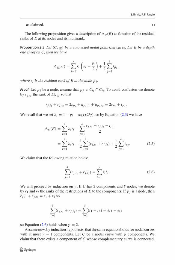
as claimed. ��The following proposition gives a description of �w(E) as function of the residual

ranks of E at its nodes and its multirank.

Proposition 2.5 Let (C, w) be a connected nodal polarized curve. Let E be a depthone sheaf on C, then we have

�w(E) =γ∑

i=1

ri

(λi − δi

2

)+ 1

2

δ∑

j=1

tp j ,

where t j is the residual rank of E at the node p j .

Proof Let p j be a node, assume that p j ∈ Ci1 ∩ Ci2 . To avoid confusion we denoteby r j,ik the rank of E |Cik

so that

r j,i1 + r j,i2 = 2sp j + ap j ,i1 + ap j ,i2 = 2sp j + tp j .

We recall that we set λi = 1 − gi − wiχ(OC ), so by Equation (2.3) we have

�w(E) =γ∑

i=1

λi ri −δ∑

j=1

r j,i1 + r j,i2 − tp j

2

=γ∑

i=1

λi ri − 1

2

δ∑

j=1

(r j,i1 + r j,i2) + 1

2

δ∑

j=1

tp j . (2.5)

We claim that the following relation holds:

δ∑

j=1

(r j,i1 + r j,i2) =γ∑

i=1

riδi (2.6)

We will proceed by induction on γ . If C has 2 components and δ nodes, we denoteby r1 and r2 the ranks of the restrictions of E to the components. If p j is a node, thenr j,i1 + r j,i2 = r1 + r2 so

δ∑

j=1

(r j,i1 + r j,i2) =δ∑

j=1

(r1 + r2) = δr1 + δr2

so Equation (2.6) holds when γ = 2.Assume now, by induction hypothesis, that the same equation holds for nodal curves

with at most γ − 1 components. Let C be a nodal curve with γ components. Weclaim that there exists a component of C whose complementary curve is connected.

123

Nodal curves and polarizations with good properties

This is true since the graph �C is connected and every connected graph has a non-disconnecting vertex1. Fix an ordering of the components of C in such a way thatthis non-disconnecting curve is Cγ . By assumption, its complementary curve Cc

γ isconnected, with γ ′ = γ − 1 components with indices i = 1, . . . , γ − 1. Moreover, ithas δ′ = δ − δγ nodes and r ′

i = ri for all i = 1, . . . , γ − 1. We can write

δ∑

j=1

(r j,i1 + r j,i2) =∑

p j /∈Cγ

(r j,i1 + r j,i2) +∑

p j∈Cγ

(r j,i1 + r j,i2). (2.7)

In the first summation on the right hand side of Equation (2.7), the sum is done overthe nodes which are not on Cγ so they are exactly the nodes of Cc

γ as a nodal curve.Then, by induction hypothesis, we have

∑

p j /∈Cγ

(r j,i1 + r j,i2) =δ′∑

j=1

(r j,i1 + r j,i2) =γ ′∑

i=1

(r ′iδ

′i ).

For all i = 1, . . . , γ − 1 we denote by εi the number of points of Ci ∩ Cγ , i.e. thenodes common to Ci and Cγ . Then we have δ′

i = δi − εi , as the nodes of Ci ∩Cγ arenot nodes of Cc

γ . If εi = 0, Ci and Cγ are disjoint and δ′i = δi . So we have:

∑

p j /∈Cγ

(r j,i1 + r j,i2) =γ−1∑

i=1

ri (δi − εi ). (2.8)

In the second summation on the right hand side of Equation (2.7), the sum is doneover the δγ nodes which are on Cγ so we can write

∑

p j∈Cγ

(r j,i1 + r j,i2) =∑

Ci |Ci∩Cγ �=∅(rγ + εi ri )

as ri = r j,ik for some j if and only if Ci is one of the components through p j and thishappens one times for each of the nodes which are on both Ci and Cγ , i.e. exactly εitimes. Hence

∑

p j∈Cγ

(r j,i1 + r j,i2) = [· · · ] =∑

Ci | εi>0

rγ +∑

Ci | εi>0

εi ri +∑

Ci | εi=0

εi ri

= rγ δγ +γ−1∑

i=1

εi ri . (2.9)

1 Let G = (V,E) be a finite connected graph, with at least 3 vertices. Then one can fix P ∈ V and considerthe distance dP (Q) of Q from P , i.e. the minimum number of edges that one needs to go through in order tomake a path from P to Q. Let R ∈ V such that dP (R) = maxQ∈V dP (Q). Then R is a non-disconnectingvertex of G. Indeed, if Q ∈ V different from R, the shorthest path from P to Q cannot pass through Rotherwise dP (R) < dP (Q) and we get a contradiction.

123

S. Brivio, F. F. Favale

Then, using Equations (2.8) and (2.9), we can rewrite Equation (2.7) as

δ∑

j=1

(r j,i1 + r j,i2) =γ−1∑

i=1

ri (δi − εi ) + rγ δγ +γ−1∑

i=1

εi ri =γ∑

i=1

riδi

which concludes the proof of the claim. From Equations (2.5) and (2.6) one obtainseasily the desired result. ��

2.2 Good polarizations andmain properties

Now we will deal with a class of polarizations which will allow us to extend someproperties that hold for locally free sheaves on smooth curves to depth one sheaves onpolarized nodal curves (see Theorem 2.9). In order to do this we will use the function�w that we have studied in Sect. 2.1.

Definition 2.6 Let (C, w) be a polarized nodal curve. We say that w is a good polar-ization if �w(E) ≥ 0 for all depth one sheaves E on C and equality holds if and onlyif E is locally free.

By Lemma 2.4 (b), for any polarization w we have �w(E) = 0 for all locally freesheaves on C . Nevertheless, it can happen that �w(E) < 0 for a depth one sheafwhich is not locally free, as the next example shows.

Example 2.7 Let (C, w) be a polarized nodal curve with two smooth components C1and C2 of genus 2 and a single node. Then �w(OC1) = −1 + 3w1. If we consider

the polarization w =(16 ,

56

), we have �w(OC1) = −1/2 < 0. Moreover, by Propo-

sition 1.4, this also implies that OC is a w-unstable sheaf on C .

First of all we will see that on all stable nodal curves with pa(C) ≥ 2 there existsa good polarization (we will see in Remark 2.13 that is not true in general).

Proposition 2.8 Let C be a stable connected nodal curve with pa(C) ≥ 2 and let be η

be the polarization induced by ωC (this is often called canonical polarization). Then,η is a good polarization on C.

Proof First of all, since C is a stable curve, we have that ωC is an ample line bundle sothe definition of η makes sense. As recalled in Sect. 1 we have ωC |Ci = ωCi ⊗ (�i )

so we have

ηi = gi − 1 + δi/2

pa(C) − 1, i = 1, . . . γ .

In order to see that η is good we will compute �η(E) for a depth one sheaf E . Forthe canonical polarization we have

λi = 1 − gi − ηiχ(OC ) = δi/2,

123

Nodal curves and polarizations with good properties

so, by Proposition 2.5 we can conclude that

�η(E) = 1

2

δ∑

j=1

tp j .

In particular, �η(E) ≥ 0 and equality holds if and only if tp j = 0 for all j . ByRemark 2.3, this happens if and only if E is locally free. ��

The following theorem summarizes some important properties which hold whenwe deal with good polarizations. Recall that Pic0(C) is the variety parametrizing linebundles having degree 0 on each component (see Sect. 1).

Theorem 2.9 Let C be a nodal curve and w a good polarization on it. Let E be adepth one sheaf on C. Then we have the following properties:

(a) Assume that E is locally free and, for i = 1, . . . , γ , Ei is stable with deg(Ei ) = 0.Then E is w-stable.

(b) If E is globally generated, then degw(E) ≥ 0.

(c) If E is w-semistable and degw(E) > 0, then h0(E∗) = 0.

In particular, if E = OC or more generally E ∈ Pic0(C) then, E is w-stable.

Proof (a) Let E be a locally free sheaf such that Ei is stable and deg(Ei ) = 0 for alli = 1, . . . , γ . Then, by Lemma 2.4 (b) we have degw(E) = 0. In order to provethat E is w-stable it is enough to show that for any proper subsheaf F of E wehave degw(F) < 0.Let F be a proper subsheaf of E and let’s consider the quotient Q = E/F . Ifrkw(Q) = 0, then Q is a torsion sheaf with finite support. Then degw(Q) =∑

P∈Supp(Q) l(QP ) > 0 and then degw(F) < 0 as claimed.Assume now that rkw(Q) > 0. Since F is a proper subsheaf of E we also haverkw(Q) < rkw(E). We define Q′ = Q/Tors(Q) which is a depth one sheaf withrkw(Q′) = rkw(Q) and degw(Q) ≥ degw(Q′). Moreover, as Q′ is a quotient ofQ we have that Q′ is a proper quotient of E . So for all i = 1, . . . , γ , we have asurjective map qi : Ei → Q′

i . If Q′i is not zero, then either qi is an isomorphism

(this cannot occur for all i) or Q′i is a proper quotient, in this case deg(Q′

i ) >

deg(Ei ) = 0 by the stability assumption on Ei . Hence∑

i deg(Q′i ) > 0. Then, as

w is a good polarization, we have

�w(Q′) = degw(Q′) −∑

i

deg(Q′i ) ≥ 0

which implies degw(Q′) > 0. Then degw(Q) > 0 and we can conclude as in theprevious case.From (a), if E is a line bundle with deg(Ei ) = 0 for all i = 1, . . . , γ , we havethat E is w-stable. One can also prove this fact directly using Proposition 1.4 bychecking that degw(L|B) > 0 for any proper subcurve B. Indeed, we have

degw(L|B) = �w(L|B) > 0,

123

S. Brivio, F. F. Favale

as w is a good polarization and L|B is not locally free on C .(b) Assume that E is a depth one sheaf on C which is generated by k ≥ 1 global

sections. Then we have a surjective map V ⊗ OC → E , where V ⊆ H0(E)

is a vector space of dimension k. Since by (a), OC is w-stable, then V ⊗ OC is

w-semistable. So we havedegw(E)

rkw(E)≥ 0 and then degw(E) ≥ 0.

(c) Assume that H0(E∗) = Hom(E,OC ) �= 0. Then, there exists a non zero homo-morphism ϕ : E → OC . We will show that degw(E) < 0. If ϕ is surjective orinjective, we conclude by w-semistability of E and by w-stability of OC (whichholds by (a), since w is good) respectively. We can assume then, that Im(ϕ) is aproper subsheaf of OC and a proper quotient of E . In this case we have

degw(E)/rkw(E) ≤ degw(Im(ϕ))/rkw(Im(ϕ)) < 0

where we used the w-semistability of E and the w-stability of OC respectively. ��Remark 2.10 In point (a) of Theorem 2.9 if Ei is only semistable then, with the samearguments, one obtain that E is w-semistable.

Another interesting consequence of the previous theorem is the following corollary.

Corollary 2.11 Let C be a nodal curve andw a good polarization. Ifw = wL for someample line bundle L,w-(semi)stability is preserved by tensoring with L. In particular,L is w-stable.

Proof Let L be a line bundle which induces the polarization wL , with Li ∈ Picdi (Ci ).Since wi = di/d then we have

wi d j = w j di .

This implies, by [24], that wL -stability is preserved by tensoring with L . In particular,since OC is wL -stable by Theorem 2.9, then L is wL -stable too. ��

2.3 Polarizations andw-stability ofOC

In this subsection we investigate polarized nodal curves (C, w) with w-stable OC .

Lemma 2.12 Let (C, w) be a polarized nodal curve. Then OC is w-stable if and onlyif

0 < �w(OB) < δB (2.10)

for any proper subcurve B of C. If equality holds for some subcurve B then OC isw-semistable. Moreover we can specialize the result in the following cases:

• If pa(C) = 0, then OC is always w-stable;• If pa(C) = 1, then OC is always w-semistable and it is w-stable if and only if Cis a cycle of rational curves;

123

Nodal curves and polarizations with good properties

• If pa(C) ≥ 2, then OC is w-stable if and only the conditions

(�)B : pa(B) − 1

pa(C) − 1< rkw(OB) <

pa(B) − 1 + δB

pa(C) − 1(2.11)

hold for all proper subcurves B of C.

Actually, it is enough to check the the Inequalities (2.10) and (2.11) only for connectedsubcurves.

Proof By Proposition 1.4 we have that OC is w-stable if and only if degw(OB) > 0for any proper subcurve B of C . Moreover, since degw(OB) = �w(OB), byLemma 2.4(e), it is enough to check the condition degw(OB) > 0 only for connectedsubcurves.

Let B be a proper subcurve of C and Bc its complementary curve. Then OB andOBc are two depth one sheaves on C . We have

degw(OB) = χ(OB) − rkw(OB)χ(OC ) = 1 − pa(B) − rkw(OB)χ(OC ).

From Equation (1.2) we have χ(OBc ) = χ(OC ) − χ(OB) + δB , so

degw(OBc ) = χ(OBc ) − rkw(OBc )χ(OC )

= χ(OC ) − χ(OB) + δB − (1 − rkw(OB))χ(OC )

= rkw(OB)χ(OC ) + pa(B) − 1 + δB .

Hence OC is w-stable if and only if both the above values are strictly positive, weobtain Inequality (2.10). If pa(C) ≥ 2, solving the inequalities we get condition (�)B .

Assume now pa(C) = 0. Then C is a curve of compact type whose componentsare rational. Then, if B is a proper connected subcurve of C , we have that B isalso of compact type. In particular pa(B) = 0 too. By Inequality (2.10) we get1 − δB < rkw(OB) < 1, so OC is w-stable.

Assume now pa(C) = 1. Then Inequality (2.10) is equivalent to 1−δB < pa(B) <

1. Since pa(B) ≤ 1 and pa(B) ≥ 1 − δB we have that OC is always w-semistable.Now we investigate the w-stability of OC . As pa(C) = 1, we have either C is ofcompact type whose components consist of an elliptic curve C1 and γ − 1 rationalcurves or the dual graph has a single cycle and all components are rationals. In thefirst case, pa(C1) = 1 so OC is never w-stable. In the second case, if we can find aproper connected subcurve B of C which contains a cycle then pa(B) = 1 andOC isnever w-stable. This happens exactly when C is not a cycle. If C is a cycle and B is aproper connected subcurve, then δB = 2 and pa(B) = 0 so OC is w-stable. ��Remark 2.13 Let C be a nodal curve with pa(C) = 1 which is not a cycle. Then goodpolarizations do not exist on C .

Remark 2.14 Assume that (C, w) is a polarized nodal curve of compact type. We cantranslate the conditions of w-stability forOC , given by Teixidor i Bigas in [25], usingour notation as follows:OC is w-stable if and only if 0 < �w(OAi ) < 1 for a suitablefamily of connected subcurves Ai ⊂ C .

123

S. Brivio, F. F. Favale

Corollary 2.15 Let w be a good polarization on a nodal curve C with pa(C) ≥ 2.Then w satisfies (�)B for all B subcurve of C. In particular, we have

gi − 1

pa(C) − 1< wi <

gi − 1 + δi

pa(C) − 1.

An interesting question is then the following:

Question 2.16 Are all polarizations for which OC is w-stable also good?

We will give a complete answer for curves of compact type in Sect. 3.

2.4 Polarizations and balanced line bundles

In this subsectionwe deal with polarized curves (C, wL)wherewL is induced by a linebundle L . We highlight the relation between the wL -stability of OC and a particularclass of line bundles: balanced line bundles (for details one can see [15,16]).

Definition 2.17 Let C be a quasistable curve of arithmetic genus pa(C) ≥ 2. A linebundle L on C is said to be balanced if the following properties hold:

(1) for every exceptional component E of C we have degE (L) = 1;(2) for any proper subcurve B we have

∣∣∣∣degB(L) − deg(L)

2pa(C) − 2degB(ωC )

∣∣∣∣ ≤ 1

2δB . (2.12)

L is said to be strictly balanced if the inequality is strict for every subcurve B suchthat B ∩ Bc is not contained in the exceptional locus of C .

Proposition 2.18 LetC beaquasistable nodal curvewith pa(C) ≥ 2. Let L ∈ Picd(C)

be an ample line bundle and let w = wL be the polarization induced by L.

(a) If d ≥ pa(C) − 1 and L is balanced, then OC is w-semistable and it is w-stablewhen d > pa(C) − 1;

(b) if d ≤ pa(C) − 1 and OC is w-stable then C is stable and L is strictly balanced.

Proof Let L ∈ Picd(C) be an ample line bundle. Then di = deg(Li ) > 0 for all i andd = ∑γ

i=1 di . As w is induced by L , we have wi = did , for all i = 1, . . . γ . Let B be

a subcurve of C . Then B = ⋃bk=1 Cik . Since L|B is a line bundle on B, we have:

degB(L) =b∑

k=1

dik =b∑

k=1

wik d = drkw(OB),

moreover we recall that

degB(ωC ) = 2pa(B) − 2 + δB .

123

Nodal curves and polarizations with good properties

We have:∣∣∣∣degB(L) − d

2pa(C) − 2degB(ωC )

∣∣∣∣ (2.13)

=∣∣∣∣drkw(OB) − d

pa(C) − 1(pa(B) − 1 + δB/2)

∣∣∣∣

= d

pa(C) − 1

∣∣(pa(C) − 1)rkw(OB) − (pa(B) − 1 + δB/2)∣∣ .

Note that condition (�)B in Lemma 2.12 can be also written as

pa(B) − 1 < (pa(C) − 1)rkw(OB) < pa(B) − 1 + δB,

which is equivalent to

∣∣(pa(C) − 1)rkw(OB) − (pa(B) − 1 + δB/2)∣∣ < δB/2.

(a) Let d ≥ pa(C) − 1 and assume that L is balanced. Then Equations (2.12) and(2.13) imply

∣∣(pa(C) − 1)rkw(OB) − (pa(B) − 1 + δB/2)∣∣ ≤ δB

2

pa(C) − 1

d.

If d > pa(C) − 1, we get

∣∣(pa(C) − 1)rkw(OB) − pa(B) + 1 − δB/2∣∣ < δB/2,

which is equivalent to (�)B . This implies that OC is w-stable. If d = pa(C) − 1, weget

∣∣(pa(C) − 1)rkw(OB) − pa(B) + 1 − δB/2∣∣ ≤ δB/2,

so we can conclude that OC is w-semistable.(b) Let d ≤ pa(C) − 1 and assume that OC is w-stable. Then w satisfies (�)B for

all subcurve B. Let R be a rational component of C , since (�)R holds, we have:

−1 < (pa(C) − 1)wR < δR − 1.

We recall that wR = dRd and dR ≥ 1 since L is ample. So we have:

1 ≤ dR <d

pa(C) − 1(δR − 1),

as d ≤ pa(C) − 1 we obtain 1 ≤ dR < δR − 1. This implies δR ≥ 3, so C is a stablecurve.

123

S. Brivio, F. F. Favale

Now we prove that L is strictly balanced. Since d ≤ pa(C) − 1 we have

∣∣∣∣degB(L) − d

2pa(C) − 2degB(ωC )

∣∣∣∣ <d

(pa(C) − 1)

δB

2≤ δB

2

by Inequality (2.13). This proves that L is strictly balanced. ��Corollary 2.19 Let C be a stable nodal curve with pa(C) ≥ 2. Let L be an ample linebundle of degree pa(C) − 1 and wL be the polarization induced by L on C. Then Lis strictly balanced if and only if OC is wL-stable.

Proof SinceC is stable, the exceptional locus ofC is empty. Moreover, as we assumeddeg(L) = pa(C) − 1, Condition (2.12) is equivalent to (�B). This implies the claim.

��

3 Good polarizations andw-Stability ofOC

Let (C, w) be a polarized nodal curve. In this section we will obtain sufficient condi-tions for a polarizationw to be good (see Theorem 3.9). Recall that, by Corollary 2.15,any good polarization satisfies properties (�)B of Lemma 2.12, or equivalently, is suchthat OC is w-stable. We will show that for curves of compact type, w-stability of OC

is also sufficient in order to have w good (see Theorem 3.10).With this aim, we will give a description of �w(E) as a function depending only

on the residual ranks and on the contribution of the non-free part of the stalks of E atnodes of C . We will get this description by considering paths on the dual graph of C ,as follows.

Assume that C has γ irreducible components and δ nodes. Let C1, . . . ,Cγ denotethe smooth components of C and p1, . . . , pδ denote the nodes of C . Let �C = (V, E)

be the dual graph of C . It is a finite graph with γ = #V vertices and δ = #E edges.Since C is connected the same holds for �C .

Notations 3.1Given a path γ in �C , we will denote by L(γ ) ∈ N the length of γ i.e. the number ofedges which are part of γ . A path has length 0 if and only if it is the trivial path. A pathjoining Ci with C j is saidminimal if it has minimal length among all the paths joiningCi and C j . As the graph �C is connected and finite, minimal paths exist for each pairof vertices. Two edges of�C are said equivalent if and only if the corresponding nodeslie on the same two components, i.e. if they connect the same vertices of �C .

A marking M is a subset of E which is a transversal for the above equivalencerelation, i.e. every edge of �C is equivalent to exactly one edge in M. The subgraph�MC = (V,M) has the same vertices of �C , is connected and it is also simple (i.e.

for each pair of vertices there is at most one edge).For our construction wewill need to fix arbitrarily a component of C. For simplicity,

we will use Cγ . We define P as any set satisfying the following properties:

(1) the elements of P are minimal paths in �MC connecting a vertex Ci to Cγ ;

123

Nodal curves and polarizations with good properties

(2) for each Ci there exists exactly one path in P starting from Ci , which we will bedenoted by γi ;

(3) if γi ∈ P and C j is a vertex on γi , then γ j is a restriction of γi .

We will call P a set of minimal paths of �C . In order to simplify the notations, ifC j ∈ V, pk ∈ E we will write pk ⊆ γi if and only if pk is an edge on γi and C j ∈ γiif and only if C j is a vertex on γi . We setM′ the subset ofM which consists of all theedges on some path in P .

If γi ∈ P and p j ⊆ γi is a node in Ck1 ∩ Ck2 , we say that Ck1 precedes Ck2 withrespect to γi if and only if, compared to Ck2 , Ck1 is closer to Ci along the path γi .

Indeed, this does not depend on the choice of γi ∈ P passing through p j as thenext lemma shows.

Lemma 3.2 Assume that γi1 and γi2 are two minimal paths ending in Cγ , which passthrough p j ∈ M with p j ∈ Ck1 ∩ Ck2 . Then the curve Ck1 precedes Ck2 with respectto γi1 if and only if the same happens with respect to γi2 .

Proof Assume, by contradiction, thatCk1 precedes Ck2 with respect to γi1 and followsCk2 with respect to γi2 . For all l = 1, 2, we denote by γ ′

ilthe path obtained by γil

by removing all the edges before p j and by γ ′′ilthe path obtained by γ ′

ilwere we

have removed also p j . Hence, γ ′i1and γ ′′

i2are both minimal paths (since minimality

is preserved by restriction) which start from Ck1 and end in Cγ . Similarly, γ ′i2and γ ′′

i1are both minimal paths connecting Ck2 and Cγ . As two minimal path joining the samevertices must have the same length we have

{L(γ ′

i1) = L(γ ′′

i2) = L(γ ′

i2) − 1

L(γ ′i2) = L(γ ′′

i1) = L(γ ′

i1) − 1

which is clearly impossible. ��Definition 3.3 Let p j ∈ E corresponding to a node in Ck1 ∩ Ck2 . If p j is equivalentto an edge which is on a path γi ∈ P we say that Ck1 precedes Ck2 if and only if Ck1precedes Ck2 with respect to γi . If p j is not equivalent to any edge on a path γi ∈ P ,we choose arbitrarily one of the two possible cases (Ck1 precedes Ck2 or Ck2 precedesCk1 ) making the same choice for equivalent edges.

Lemma 3.2 ensures that the above definition is well posed. This gives the structureof oriented graph to �C and to its subgraph �M

C .

Notations 3.4Let E be a depth one sheaf on C. Let p j be a node with p j ∈ Ck1 ∩ Ck2 . Denote byq j,k1 and q j,k2 the points of Ck1 and Ck2 respectively on the normalization of C whichare glued together in order to obtain p j . We recall that we have integers s j , a j,k1 anda j,k2 such that

Ep j = Os jp j ⊕ Oa j,k1

q j,k1⊕ Oa j,k2

q j,k2,

123

S. Brivio, F. F. Favale

and satisfying rkl = s j + a j,kl for l = 1, 2. We set

a j := a j,k1 and b j := a j,k2 ⇐⇒ Ck1 precedes Ck2 (3.1)

and the opposite in the other case. In particular, we have that a j + b j = tp j .

Lemma 3.5 Let E be any depth one sheaf on C. Then

(a) if pl and p j are equivalent edges, we have bl − al = b j − a j ;(b) if γi ∈ P then we have

∑p j⊆γi

(b j − a j ) = rγ − ri .

Proof (a) Let E be a depth one sheaf. Let p j and pl be two equivalent edges. Thenp j , pl ∈ Ck1 ∩ Ck2 . Without loss of generality we can assume that Ck1 precedesCk2 . Then

rk1 = s j + a j = sl + al rk2 = s j + b j = sl + bl ,

so al − a j = s j − sl = bl − b j and then bl − al = b j − a j as claimed.(b) Let γi ∈ P .Wewill prove the formula by induction on the lenght of γi . If L(γi ) = 1

then γi is a single edge (say p j ) joining the vertices Ci and Cγ . Then ri =s j + a j , rγ = s j + b j so rγ − ri = b j − a j as claimed. Now assume that theformula is true for any minimal path of lenght at most L and consider a minimalpath γi of lenght L + 1. Let pl be the first edge, and denote by Ck the secondvertex on the path (the first is Ci ). If we remove pl from the path we get, by thedefinition of P the minimal path γk joining Ck to Cγ which has length L . So, byinduction, we have

rγ − rk =∑

p j⊆γk

(b j − a j ).

On the other hand we have ri = sl + al , rk = sl + bl so rk − ri = bl − al and wehave

rγ − ri = (rk − ri ) + (rγ − rk) = (bl − al) +∑

p j⊆γk

(b j − a j ) =∑

p j⊆γi

(b j − a j )

as claimed.��

By Lemma 3.5(a) it follows that the choice of the marking M does not influencethe relation in Lemma 3.5(b).

Definition 3.6 Assume that a marking M and a set P of minimal paths on �C (asin Notation 3.1) have been chosen. Then, for any p j ∈ M, we define A j to be thesubcurve of C with the following property: Ci is a component of A j if and only ifp j ⊆ γi .

123

Nodal curves and polarizations with good properties

Note that A j could be empty for same j : this occurs exactly when p j /∈ M′.Before stating the main result of this section, we will need the following technical

result:

Lemma 3.7 Let A j ⊆ C be as in Definition 3.6 and assume that A j is not empty. Then

(a) A j is a proper connected subcurve of C;(b) Ac

j is connected;

(c)∑

Ci⊆A j

(λi − δi

2

)= 1− pa(A j )+(pa(C)−1)rkw(OA j )− 1

2δA j = �w(OA j )−12δA j ;

(d) if C is of compact type, then δA j = 1.

Proof (a) Consider a componentCi of A j . Then the pathγi passes through p j . Assumethat p j ∈ Ck1 ∩ Ck2 and that Ck1 precedes Ck2 . Let Cl be a vertex on γi which isbetween Ci and Ck1 (included). Then γl is the restriction of γi and p j is an edgein γl . In particular, Cl is a component of A j . This shows that Ci is connected toCk1 using only curves in A j so A j is connected. Properness follows as Ck2 cannotbe a component of A j .

(b) It is enough to show that if Ci is a component not in A j then there is a path in �C

fromCi toCγ which only passes through verticeswhich correspond to componentsnot in A j . The path γi connects Ci with Cγ . Assume, by contradiction, that oneof the vertex on the path γi , say Ck , is a component of A j . Then, the restriction ofγi from Ck to Cγ is γk . Since Ck is a component of A j we have that p j ⊂ γk , sothe same is true for γi . But this is impossible as we assumed that Ci /∈ A j .

(c) We denote by C(A j ) and N (A j ) the number of components and of nodes respec-tively of the curve A j . We recall that δA j = A j · Ac

j is the number of nodes of Clying on A j which are not nodes of A j . Then we have

∑

Ci⊆A j

(λi − δi

2

)=

∑

Ci⊆A j

[1 − gi + wi (pa(C) − 1)] − 1

2

∑

Ci⊆A j

δi

= C(A j ) −∑

Ci⊆A j

gi

+rkw(OA j )(pa(C) − 1) − N (A j ) − 1

2δA j

= 1 − pa(A j ) + (pa(C) − 1)rkw(OA j ) − 1

2δA j (3.2)

as A j is connected and pa(A j ) = ∑Ci⊆A j

gi + N (A j ) −C(A j ) + 1. Finally, werecall that 1 − pa(A j ) + (pa(C) − 1)rkw(OA j ) = �w(OA j ).

(d) SinceC is of compact type, by (a) and (b) it follows that A j and Acj are both curves

of compact type too. From Equation (1.3) we have:

γ∑

i=1

gi =∑

Ci⊆A j

gi +∑

Ci⊆Acj

gi + δA j − 1,

123

S. Brivio, F. F. Favale

which implies δA j = 1. ��Remark 3.8 We point out that, if C is of compact type, the family of connected curves{A j }, defined in Definition 3.6, can be used to obtain the conditions of w-stability in[25] (see also Remark 2.14).

We are now able to state our first result of this section:

Theorem 3.9 Let (C, w) be a polarized nodal curve. Fix a marking M on the dualgraph �C and a set of minimal path P as in Notations 3.1. Then for any depth onesheaf E we have:

�w(E) =∑

p j∈M′

[a j

(1

2(1 − δA j ) + �w(OA j )

)+ b j

(1

2(1 + δA j ) − �w(OA j )

)]

+1

2

∑

p j /∈M′(a j + b j ).

In particular, if the conditions

(��)A j : 1

2(δA j − 1) < �w(OA j ) <

1

2(δA j + 1) (3.3)

hold for all the non-empty subcurves A j then w is a good polarization.

Proof We start from the expression of �w(E) given by Proposition 2.5. Then, usingLemma 3.5(b) we have

�w(E) =γ∑

i=1

ri

(λi − δi

2

)+ 1

2

δ∑

j=1

tp j

=γ∑

i=1

⎛

⎝rγ +∑

p j⊆γi

(a j − b j )

⎞

⎠(

λi − δi

2

)+ 1

2

δ∑

j=1

tp j

= rγ

γ∑

i=1

(λi − δi

2

)+

γ∑

i=1

∑

p j⊆γi

(a j − b j )

(λi − δi

2

)+ 1

2

δ∑

j=1

tp j .

By Lemma 2.4(a) we have that the coefficient of rγ in the last equality is 0 so �w(E)

is equal to

γ∑

i=1

∑

p j⊆γi

(a j − b j )

(λi − δi

2

)+ 1

2

δ∑

j=1

(a j + b j )

=δ∑

j=1

(a j − b j )∑

γi⊇p j

(λi − δi

2

)+ 1

2

δ∑

j=1

(a j + b j )

123

Nodal curves and polarizations with good properties

=∑

p j∈M′

⎡

⎣a j

⎛

⎝1

2+

∑

γi⊇p j

(λi − δi

2

)⎞

⎠ + b j

⎛

⎝1

2−

∑

γi⊇p j

(λi − δi

2

)⎞

⎠

⎤

⎦

+1

2

∑

p j /∈M′(a j + b j )

since, if p j /∈ M′ the sum over the path passing through p j is trivial. If p j ∈ M′, thecondition γi ⊇ p j is equivalent to Ci ∈ A j so, by Lemma 3.7(c) we have

�w(E) =∑

p j∈M′

[a j

(1

2+ �w(OA j ) − δA j

2

)+ b j

(1

2− �w(OA j ) + δA j

2

)]

+1

2

∑

p j /∈M′(a j + b j )

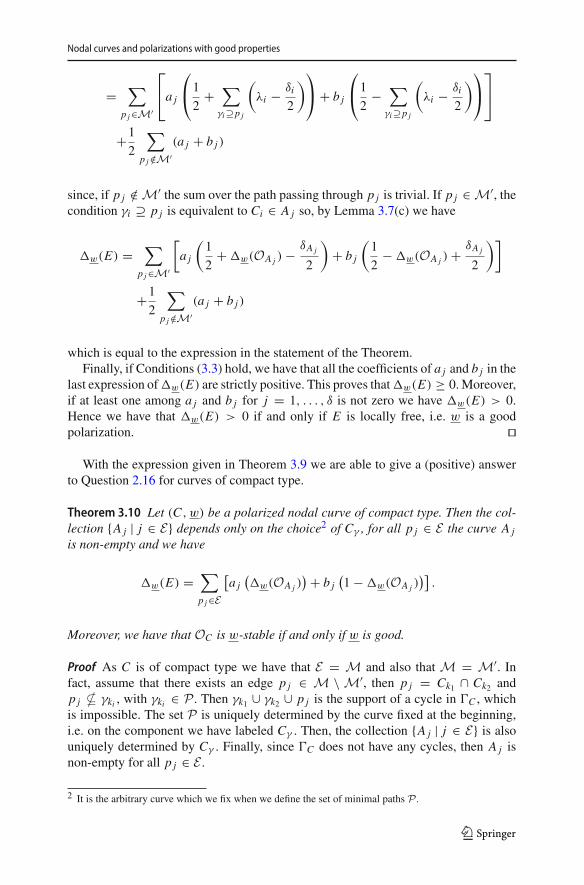
which is equal to the expression in the statement of the Theorem.Finally, if Conditions (3.3) hold, we have that all the coefficients of a j and b j in the

last expression of�w(E) are strictly positive. This proves that�w(E) ≥ 0.Moreover,if at least one among a j and b j for j = 1, . . . , δ is not zero we have �w(E) > 0.Hence we have that �w(E) > 0 if and only if E is locally free, i.e. w is a goodpolarization. ��

With the expression given in Theorem 3.9 we are able to give a (positive) answerto Question 2.16 for curves of compact type.

Theorem 3.10 Let (C, w) be a polarized nodal curve of compact type. Then the col-lection {A j | j ∈ E} depends only on the choice2 of Cγ , for all p j ∈ E the curve A j

is non-empty and we have

�w(E) =∑

p j∈E

[a j

(�w(OA j )

) + b j(1 − �w(OA j )

)].

Moreover, we have that OC is w-stable if and only if w is good.

Proof As C is of compact type we have that E = M and also that M = M′. Infact, assume that there exists an edge p j ∈ M \ M′, then p j = Ck1 ∩ Ck2 andp j � γki , with γki ∈ P . Then γk1 ∪ γk2 ∪ p j is the support of a cycle in �C , whichis impossible. The set P is uniquely determined by the curve fixed at the beginning,i.e. on the component we have labeled Cγ . Then, the collection {A j | j ∈ E} is alsouniquely determined by Cγ . Finally, since �C does not have any cycles, then A j isnon-empty for all p j ∈ E .

2 It is the arbitrary curve which we fix when we define the set of minimal paths P .

123

S. Brivio, F. F. Favale

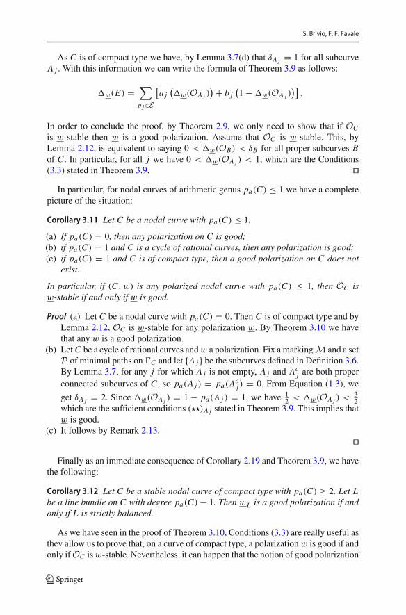
As C is of compact type we have, by Lemma 3.7(d) that δA j = 1 for all subcurveA j . With this information we can write the formula of Theorem 3.9 as follows:

�w(E) =∑

p j∈E

[a j

(�w(OA j )

) + b j(1 − �w(OA j )

)].

In order to conclude the proof, by Theorem 2.9, we only need to show that if OC

is w-stable then w is a good polarization. Assume that OC is w-stable. This, byLemma 2.12, is equivalent to saying 0 < �w(OB) < δB for all proper subcurves Bof C . In particular, for all j we have 0 < �w(OA j ) < 1, which are the Conditions(3.3) stated in Theorem 3.9. ��

In particular, for nodal curves of arithmetic genus pa(C) ≤ 1 we have a completepicture of the situation:

Corollary 3.11 Let C be a nodal curve with pa(C) ≤ 1.

(a) If pa(C) = 0, then any polarization on C is good;(b) if pa(C) = 1 and C is a cycle of rational curves, then any polarization is good;(c) if pa(C) = 1 and C is of compact type, then a good polarization on C does not

exist.

In particular, if (C, w) is any polarized nodal curve with pa(C) ≤ 1, then OC isw-stable if and only if w is good.

Proof (a) Let C be a nodal curve with pa(C) = 0. Then C is of compact type and byLemma 2.12, OC is w-stable for any polarization w. By Theorem 3.10 we havethat any w is a good polarization.

(b) LetC be a cycle of rational curves andw a polarization. Fix a markingM and a setP of minimal paths on �C and let {A j } be the subcurves defined in Definition 3.6.By Lemma 3.7, for any j for which A j is not empty, A j and Ac

j are both properconnected subcurves of C , so pa(A j ) = pa(Ac

j ) = 0. From Equation (1.3), we

get δA j = 2. Since �w(OA j ) = 1 − pa(A j ) = 1, we have 12 < �w(OA j ) < 3

2which are the sufficient conditions (��)A j stated in Theorem 3.9. This implies thatw is good.

(c) It follows by Remark 2.13.��

Finally as an immediate consequence of Corollary 2.19 and Theorem 3.9, we havethe following:

Corollary 3.12 Let C be a stable nodal curve of compact type with pa(C) ≥ 2. Let Lbe a line bundle on C with degree pa(C) − 1. Then wL is a good polarization if andonly if L is strictly balanced.

As we have seen in the proof of Theorem 3.10, Conditions (3.3) are really useful asthey allow us to prove that, on a curve of compact type, a polarization w is good if andonly ifOC isw-stable. Nevertheless, it can happen that the notion of good polarization

123

Nodal curves and polarizations with good properties

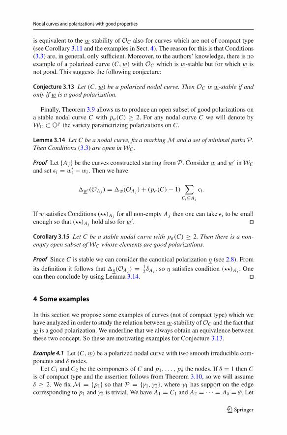
is equivalent to the w-stability of OC also for curves which are not of compact type(see Corollary 3.11 and the examples in Sect. 4). The reason for this is that Conditions(3.3) are, in general, only sufficient. Moreover, to the authors’ knowledge, there is noexample of a polarized curve (C, w) with OC which is w-stable but for which w isnot good. This suggests the following conjecture:

Conjecture 3.13 Let (C, w) be a polarized nodal curve. Then OC is w-stable if andonly if w is a good polarization.

Finally, Theorem 3.9 allows us to produce an open subset of good polarizations ona stable nodal curve C with pa(C) ≥ 2. For any nodal curve C we will denote byWC ⊂ Q

γ the variety parametrizing polarizations on C .

Lemma 3.14 Let C be a nodal curve, fix a markingM and a set of minimal paths P .Then Conditions (3.3) are open inWC .

Proof Let {A j } be the curves constructed starting from P . Consider w and w′ inWC

and set εi = w′i − wi . Then we have

�w′(OA j ) = �w(OA j ) + (pa(C) − 1)∑

Ci⊆A j

εi .

If w satisfies Conditions (��)A j for all non-empty A j then one can take εi to be smallenough so that (��)A j hold also for w′. ��Corollary 3.15 Let C be a stable nodal curve with pa(C) ≥ 2. Then there is a non-empty open subset of WC whose elements are good polarizations.

Proof Since C is stable we can consider the canonical polarization η (see 2.8). From

its definition it follows that �η(OA j ) = 12δA j , so η satisfies condition (��)A j . One

can then conclude by using Lemma 3.14. ��

4 Some examples

In this section we propose some examples of curves (not of compact type) which wehave analyzed in order to study the relation betweenw-stability ofOC and the fact thatw is a good polarization. We underline that we always obtain an equivalence betweenthese two concept. So these are motivating examples for Conjecture 3.13.

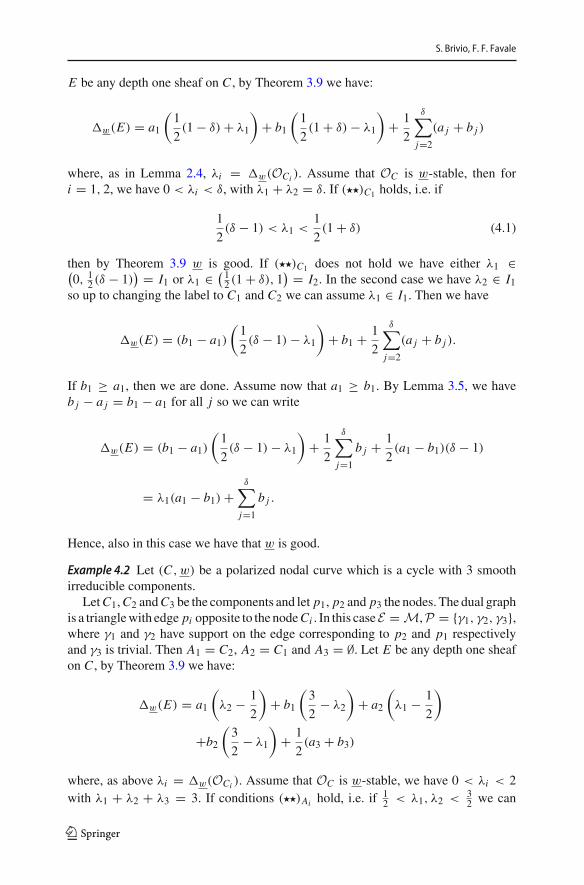
Example 4.1 Let (C, w) be a polarized nodal curve with two smooth irreducible com-ponents and δ nodes.

Let C1 and C2 be the components of C and p1, . . . , pδ the nodes. If δ = 1 then Cis of compact type and the assertion follows from Theorem 3.10, so we will assumeδ ≥ 2. We fix M = {p1} so that P = {γ1, γ2}, where γ1 has support on the edgecorresponding to p1 and γ2 is trivial. We have A1 = C1 and A2 = · · · = Aδ = ∅. Let

123

S. Brivio, F. F. Favale

E be any depth one sheaf on C , by Theorem 3.9 we have:

�w(E) = a1

(1

2(1 − δ) + λ1

)+ b1

(1

2(1 + δ) − λ1

)+ 1

2

δ∑

j=2

(a j + b j )

where, as in Lemma 2.4, λi = �w(OCi ). Assume that OC is w-stable, then fori = 1, 2, we have 0 < λi < δ, with λ1 + λ2 = δ. If (��)C1 holds, i.e. if

1

2(δ − 1) < λ1 <

1

2(1 + δ) (4.1)

then by Theorem 3.9 w is good. If (��)C1 does not hold we have either λ1 ∈(0, 1

2 (δ − 1)) = I1 or λ1 ∈ ( 1

2 (1 + δ), 1) = I2. In the second case we have λ2 ∈ I1

so up to changing the label to C1 and C2 we can assume λ1 ∈ I1. Then we have

�w(E) = (b1 − a1)

(1

2(δ − 1) − λ1

)+ b1 + 1

2

δ∑

j=2

(a j + b j ).

If b1 ≥ a1, then we are done. Assume now that a1 ≥ b1. By Lemma 3.5, we haveb j − a j = b1 − a1 for all j so we can write

�w(E) = (b1 − a1)

(1

2(δ − 1) − λ1

)+ 1

2

δ∑

j=1

b j + 1

2(a1 − b1)(δ − 1)

= λ1(a1 − b1) +δ∑

j=1

b j .

Hence, also in this case we have that w is good.

Example 4.2 Let (C, w) be a polarized nodal curve which is a cycle with 3 smoothirreducible components.

LetC1,C2 andC3 be the components and let p1, p2 and p3 the nodes. The dual graphis a trianglewith edge pi opposite to the nodeCi . In this caseE = M,P = {γ1, γ2, γ3},where γ1 and γ2 have support on the edge corresponding to p2 and p1 respectivelyand γ3 is trivial. Then A1 = C2, A2 = C1 and A3 = ∅. Let E be any depth one sheafon C , by Theorem 3.9 we have:

�w(E) = a1

(λ2 − 1

2

)+ b1

(3

2− λ2

)+ a2

(λ1 − 1

2

)

+b2

(3

2− λ1

)+ 1

2(a3 + b3)

where, as above λi = �w(OCi ). Assume that OC is w-stable, we have 0 < λi < 2with λ1 + λ2 + λ3 = 3. If conditions (��)Ai hold, i.e. if

12 < λ1, λ2 < 3

2 we can

123

Nodal curves and polarizations with good properties

conclude. If (��)Ai do not hold, one can prove that by exchanging the labels to C1,C2and C3 one can assume 0 < λ1 < 1

2 and 12 < λ2 < 3

2 . We can write

�w(E) = a1

(λ2 − 1

2

)+ b1

(3

2− λ2

)+

(1

2− λ1

)(b2 − a2) + b2 + 1

2(a3 + b3).

The cycle in the dual graph yields the following relation

b2 − a2 = b1 − a1 + b3 − a3.

As in the previous example using the above relation, one can prove that �w(E) ≥ 0and equality holds if and only if E is locally free, i.e. that w is good.

Acknowledgements The authors want to express their gratitude to both the anonymous referees for theirhelpful remarks and keen suggestions. They contributed a lot to the final version of this paper.

Funding Open access funding provided by Università degli Studi di Milano - Bicocca within the CRUI-CARE Agreement.

OpenAccess This article is licensedunder aCreativeCommonsAttribution 4.0 InternationalLicense,whichpermits use, sharing, adaptation, distribution and reproduction in any medium or format, as long as you giveappropriate credit to the original author(s) and the source, provide a link to the Creative Commons licence,and indicate if changes were made. The images or other third party material in this article are includedin the article’s Creative Commons licence, unless indicated otherwise in a credit line to the material. Ifmaterial is not included in the article’s Creative Commons licence and your intended use is not permittedby statutory regulation or exceeds the permitted use, you will need to obtain permission directly from thecopyright holder. To view a copy of this licence, visit http://creativecommons.org/licenses/by/4.0/.

References

1. Altman, A.S., Kleiman, S.L.: Bertini theorems for hypersurface sections containing a subscheme.Commun. Algebra 8, 775–790 (1979)

2. Arbarello, E., Cornalba, M., Griffiths, P.A.: Geometry of algebraic curves. Volume II, Grundlehrender Mathematischen Wissenschaften [Fundamental Principles of Mathematical Sciences], 268, Witha contribution by Joseph Daniel Harris, Springer, Heidelberg (2011). xxx+963

3. Beauville, A.: Theta functions, old and new, open problems and surveys of contemporary mathematics,Surv. Mod. Math., vol. 6, pp. 99–132. International Press, Somerville (2013)

4. Bhosle, U.: Generalised parabolic bundles and applications to torsionfree sheaves on nodal curves.Ark. Mat. 30(2), 187–215 (1992)

5. Bolognesi, M., Brivio, S.: Coherent systems and modular subavrieties of SUC (r). Int. J. Math. 23(4),1250037 (2012)

6. Bradlow, S.B.: Coherent systems: a brief survey, With an appendix by H. Lange, Moduli spaces andvector bundles, London Math. Soc. Lecture Note Ser., vol. 359, pp. 229–264. Cambridge UniversityPress, Cambridge (2009)

7. Bradlow, S.B., García-Prada, O., Muñoz, V., Newstead, P.E.: Coherent systems and Brill-Noethertheory. Int. J. Math. 14(7), 683–733 (2003)

8. Brivio, S., Favale, F.F.: Genus 2 curves and generalized theta divisors. Bull. Sci. Math. 155, 112–140(2019)

9. Brivio, S., Favale, F.F.: On vector bundle over reducible curves with a node, 2019, To appear inAdvances in Geometry. https://doi.org/10.1515/advgeom-2020-0010

10. Brivio, S., Favale, F.F.: On Kernel Bundle over reducible curves with a node. Int. J. Math. (2020).https://doi.org/10.1142/S0129167X20500548

123

S. Brivio, F. F. Favale

11. Brivio, S., Favale, F.F.: Coherent systems on curves of compact type. J. Geom. Phys. 158, 103850(2020)

12. Brivio, S.: A note on theta divisors of stable bundles. Rev. Mat. Iberoam. 31(2), 601–608 (2015)13. Brivio, S.: Families of vector bundles and linear systems of theta divisors. Int. J. Math. 28(6), 1750039,

16 (2017)14. Brivio, S., Verra, A.: Plücker forms and the theta map. Am. J. Math. 134(5), 1247–1273 (2012)15. Caporaso, L.: A compactification of the universal Picard variety over the moduli space of stable curves.

J. Am. Math. Soc. 7(3), 589–660 (1994)16. Caporaso, L.: Linear series on semistable curves. Int. Math. Res. Not. IMRN 13, 2921–2969 (2011)17. Esteves, E.: Compactifying the relative Jacobian over families of reduced curves. Trans. Am. Math.

Soc. 353(8), 3045–3095 (2001)18. Gieseker, D.: A degeneration of the moduli space of stable bundles. J. Differ. Geom. 19(1), 173–206

(1984)19. Gieseker, D., Morrison, I.: Hilbert stability of rank-two bundles on curves. J. Differ. Geom. 19(1), 1–29

(1984)20. King, A.D., Newstead, P.E.: Moduli of Brill-Noether pairs on algebraic curves. Int. J. Math. 6(5),

733–748 (1995)21. Le Potier, J.: Lectures on vector bundles, Cambridge Studies in Advanced Mathematics, vol. 54,

Cambridge University Press, Cambridge. Translated by A. Maciocia (1997)22. Mumford, D.: On the equations defining abelian varieties. Invent. Math. 1, 287–354 (1966)23. Oda, T., Seshadri, C.S.: Compactifications of the generalized Jacobian variety. Trans. Am. Math. Soc.

253, 1–90 (1979)24. Seshadri, C.S.: Fibrés vectoriels sur les courbes algébriques, French, Astérisque, vol. 96, Société

Mathématique de France, Paris, (1982) (French). Notes written by J.-M. Drezet from a course at theÉcole Normale Supérieure, (1980)

25. Teixidor i Bigas, M.: Moduli spaces of (semi)stable vector bundles on tree-like curves. Math. Ann.290(2), 341–348 (1991)

26. Teixidor i Bigas, M.: Moduli spaces of vector bundles on reducible curves. Am. J. Math. 117(1),125–139 (1995)

27. Teixidor i Bigas, M.: Vector bundles on reducible curves and applications, Grassmannians, modulispaces and vector bundles. Clay Math. Proc. 14, 169–180 (2011)

Publisher’s Note Springer Nature remains neutral with regard to jurisdictional claims in published mapsand institutional affiliations.

123