No Slide Titleshekhar/talk/2011/11.9... · 2011-11-17 · A Real World Testcase Source cities Destination Monticello Power Plant Routes used only by old plan Routes used only by result

Spatial Computing

Shashi Shekhar McKnight Distinguished University Professor

Department of Computer Science and Engineering

University of Minnesota

www.cs.umn.edu/~shekhar

2

Smarter

Planet

SIG

SPATIAL

Spatial Computing: Reccent Trends

Motivation for Spatial Computing

• Societal: • Google Earth, Google Maps, Navigation, location-based service

• Global Challenges facing humanity – many are geo-spatial!

• Future of Computer Science (CS) is to address societal challenges!

Governement Applications

• Spatial computing

– NASA Earth Observing System (EOS): Earth science data

– National Inst. of Justice: crime mapping

– Census Bureau, Dept. of Commerce: census data

– Dept. of Transportation (DOT): traffic data

– National Inst. of Health (NIH): cancer clusters

– Commerce, e.g. Retail Analysis

• Sample Global Questions from Earth Science

– How is the global Earth system changing

– What are the primary forcing of the Earth system

– How does the Earth system respond to natural and human induced changes

– What are the consequences of changes in the Earth system for human civilization

– How well can we predict future changes in the Earth system?

Spatial Computing in Government

Spatial thinking in Business Analytics

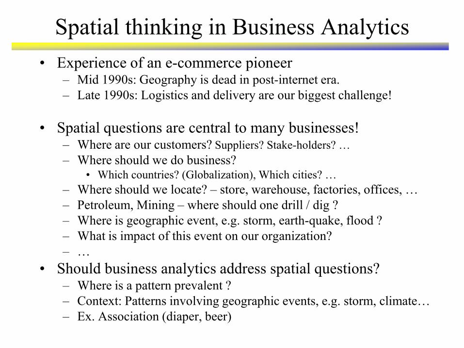
• Experience of an e-commerce pioneer – Mid 1990s: Geography is dead in post-internet era.

– Late 1990s: Logistics and delivery are our biggest challenge!

• Spatial questions are central to many businesses! – Where are our customers? Suppliers? Stake-holders? …

– Where should we do business? • Which countries? (Globalization), Which cities? …

– Where should we locate? – store, warehouse, factories, offices, …

– Petroleum, Mining – where should one drill / dig ?

– Where is geographic event, e.g. storm, earth-quake, flood ?

– What is impact of this event on our organization?

– …

• Should business analytics address spatial questions? – Where is a pattern prevalent ?

– Context: Patterns involving geographic events, e.g. storm, climate…

– Ex. Association (diaper, beer)

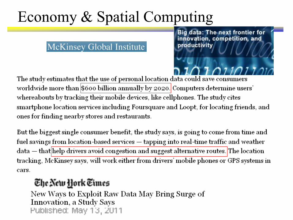
Economy & Spatial Computing

Spatial Thinking in Consumer Applications

• Trends: Consumers account for two-third of US economy

Cell phone outnumber personal computers

Spatial apps dominate the Google android app. contest winner

Research Challenges in Spatial Computing

• Is spatial computing just an application of well-known CSE techniques?

• Are there CSE research challenges and opportunities ?

• Dynamic Programming is a popular algorithm design paradigm

• Shortest Path Algorithm

• DBMS Query Optimization

• Sequence alignment,

• Viterbi algorithm, …

• However, DP assumes stationary ranking of candidate solutions

• Is DP appropriate for longitudal problems ?

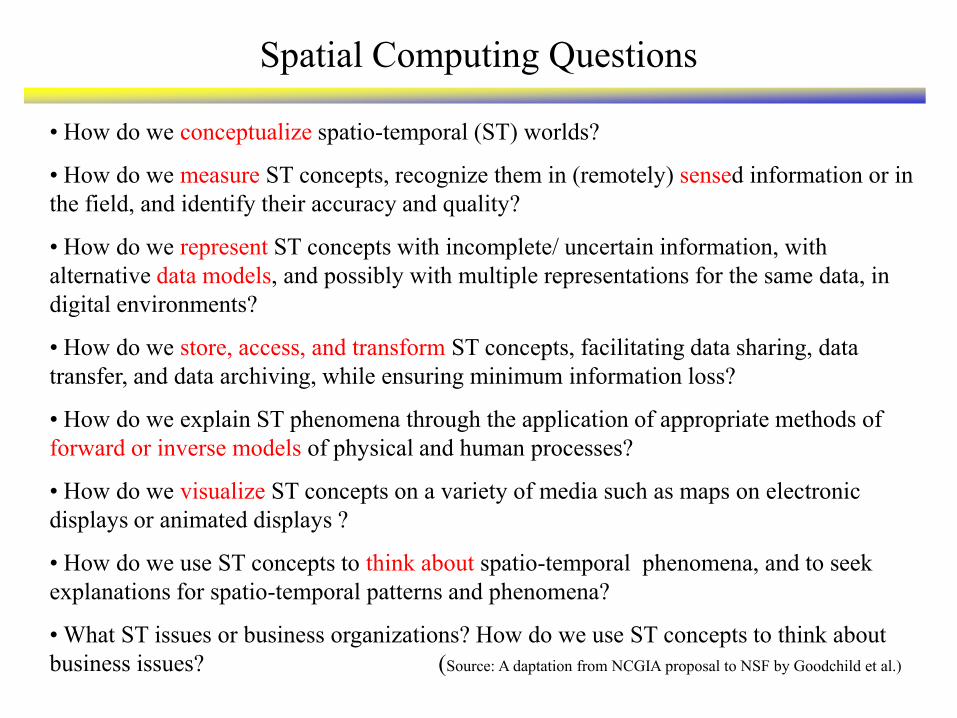
Spatial Computing Questions

• How do we conceptualize spatio-temporal (ST) worlds?

• How do we measure ST concepts, recognize them in (remotely) sensed information or in

the field, and identify their accuracy and quality?

• How do we represent ST concepts with incomplete/ uncertain information, with

alternative data models, and possibly with multiple representations for the same data, in

digital environments?

• How do we store, access, and transform ST concepts, facilitating data sharing, data

transfer, and data archiving, while ensuring minimum information loss?

• How do we explain ST phenomena through the application of appropriate methods of

forward or inverse models of physical and human processes?

• How do we visualize ST concepts on a variety of media such as maps on electronic

displays or animated displays ?

• How do we use ST concepts to think about spatio-temporal phenomena, and to seek

explanations for spatio-temporal patterns and phenomena?

• What ST issues or business organizations? How do we use ST concepts to think about

business issues? (Source: A daptation from NCGIA proposal to NSF by Goodchild et al.)

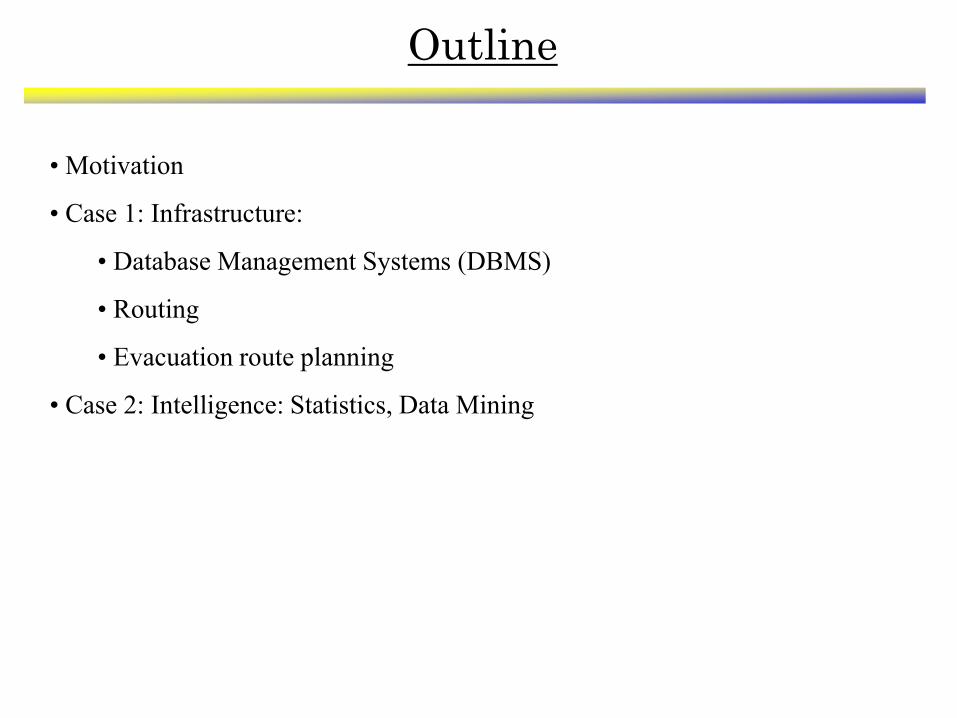
Outline

• Motivation

• Case 1: Infrastructure:

• Database Management Systems (DBMS)

• Routing

• Evacuation route planning

• Case 2: Intelligence: Statistics, Data Mining

Relational DBMS to Spatial DBMS

• 1980s: Relational DBMS • Relational Algebra

• Query Processing, e.g. sort-merge equi-join algorithm, …

• B+ Tree index

• Spatial customer (e.g. NASA, USPS) got interested

• But faced challenges

• Semantic Gap • Spatial concepts: distance, direction, overlap, inside, shortest paths, …

• SQL representation was quite verbose

• Relational algebra can not represent Transitive closure

• Performance challenge due to linearity assumption • Is B+ tree appropriate for geographic data?

• Is sorting natural in geographic space?

• New ideas emerged in 1990s • Spatial data types and operations (e.g. OGIS Simple Features)

• R-tree, space partitioning, …

Spatial Databases: Representative Projects

only in old plan

Only in new plan

In both plans

Evacutation Route Planning

Parallelize

Range Queries

Storing graphs in disk blocks Shortest Paths

Eco-Routing

U.P.S. Embraces High-Tech Delivery Methods (July 12, 2007)

By “The research at U.P.S. is paying off. ……..— saving roughly three million

gallons of fuel in good part by mapping routes that minimize left turns.”

• Minimize fuel consumption and GPG emission

– rather than proxies, e.g. distance, travel-time

– avoid congestion, idling at red-lights, turns and elevation changes, etc.

Revisit Shortest Path Problem

Time-Variant Flow Network Questions

New Routing Questions

Best start time to minimize time spend on network

Account for delays at signals, rush hour, etc.

U.P.S. Embraces High-Tech Delivery Methods (July 12, 2007)

By “The research at U.P.S. is paying off. ……..— saving roughly three million

gallons of fuel in good part by mapping routes that minimize left turns.”

RealReal--time and Historic Traveltime and Historic Travel--time Datasetstime Datasets

16

Eco-Routing: Spatial Computing Questions

• What are expected fuel saving from use of GPS devices with static roadmaps?

• What is the value-added by historical traffic and congestion information?

• How much additional value is added by real-time traffic information?

• What are the impacts of following on fuel savings and green house emissions?

– traffic management systems (e.g. traffic light timing policies),

– vehicles (e.g. weight, engine size, energy-source),

– driver behavior (e.g. gentle acceleration/braking)

– environment (e.g. weather)

• What is computational structure of the Eco-Routing problem?

• Does this problem satisfy the assumptions (e.g. stationary ranking of alternative routes)

behind common shortest-path computation algorithms?

Routing in ST Networks

Predictable

Future

Unpredictable

Future

Stationary

Non-stationary

Dijkstra’s, A*….

Broader Implication of Stationary Assumption

• Dynamic Programming is a popular algorithm design paradigm

• Shortest Path Algorithm

• DBMS Query Optimization

• Sequence alignment,

• Viterbi algorithm, …

• However, DP assumes stationary ranking of candidate solutions

• Is DP appropriate for longitudal spatial problems ?

Evacuation Route Planning - Motivation

No coordination among local plans means

Traffic congestions on all highways

e.g. 60 mile congestion in Texas (2005)

Great confusions and chaos

"We packed up Morgan City residents to evacuate in the a.m. on the day that Andrew hit coastal Louisiana, but in early afternoon the majority came back home. The traffic was so bad that they couldn't get through Lafayette." Mayor Tim Mott, Morgan City, Louisiana ( http://i49south.com/hurricane.htm )

Florida, Lousiana

(Andrew, 1992)

( www.washingtonpost.com)

( National Weather Services) ( National Weather Services)

( FEMA.gov)

I-45 out of Houston

Houston

(Rita, 2005)

A Real Scenario

Nuclear Power Plants in Minnesota

Twin Cities

Monticello Emergency Planning Zone

Monticello EPZ Subarea Population 2 4,675

5N 3,994

5E 9,645

5S 6,749

5W 2,236

10N 391

10E 1,785

10SE 1,390

10S 4,616

10SW 3,408

10W 2,354

10NW 707

Total 41,950

Estimate EPZ evacuation time:

Summer/Winter (good weather):

3 hours, 30 minutes

Winter (adverse weather):

5 hours, 40 minutes

Emergency Planning Zone (EPZ) is a 10-mile radius

around the plant divided into sub areas.

Data source: Minnesota DPS & DHS

Web site: http://www.dps.state.mn.us

http://www.dhs.state.mn.us

A Real World Testcase

Source cities

Destination

Monticello Power Plant

Routes used only by old plan

Routes used only by result plan of

capacity constrained routing

Routes used by both plans

Congestion is likely in old plan near evacuation

destination due to capacity constraints. Our plan

has richer routes near destination to reduce

congestion and total evacuation time.

Twin Cities

Experiment Result

Total evacuation time:

- Existing Plan: 268 min.

- New Plan: 162 min.

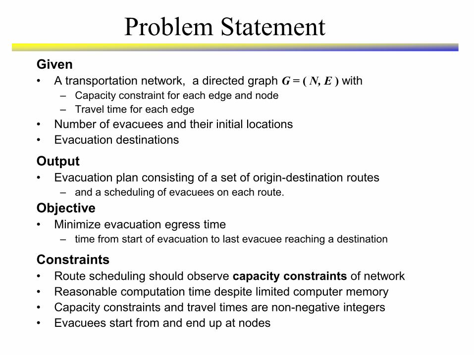
Problem Statement

Given

• A transportation network, a directed graph G = ( N, E ) with

– Capacity constraint for each edge and node

– Travel time for each edge

• Number of evacuees and their initial locations

• Evacuation destinations

Output

• Evacuation plan consisting of a set of origin-destination routes

– and a scheduling of evacuees on each route.

Objective

• Minimize evacuation egress time

– time from start of evacuation to last evacuee reaching a destination

Constraints

• Route scheduling should observe capacity constraints of network

• Reasonable computation time despite limited computer memory

• Capacity constraints and travel times are non-negative integers

• Evacuees start from and end up at nodes

Summary of Related Works & Limitations

B. Operations Research: Time-Expanded Graph + Linear Programming

- Optimal solution, e.g. EVACNET (U. FL), Hoppe and Tardos (Cornell U).

Limitation: - High computational complexity => Does not scale to large problems

- Users need to guess an upper bound on evacuation time

Inaccurate guess => either no solution or increased computation cost!

A. Capacity-ignorant Approach

- Simple shortest path computation, e.g. A*, Dijktra’s, etc.

- e.g. EXIT89 (National Fire Protection Association)

Limitation: Poor solution quality as evacuee population grows

> 5 days 108 min 2.5 min 0.1 min EVACNET Running Time

50,000 5,000 500 50 Number of Nodes

C. Transportation Science: Dynamic Traffic Assignment

- Game Theory: Wardrop Equilibrium, e.g. DYNASMART (FHWA), DYNAMIT(MIT)

Limitation: Extremely high compute time

- Is Evacuation an equilibrium phenomena?

26

Representations of (Spatio-)temporal Networks

t=1

N2

N1

N3

N4 N5

1

2

2

2

t=2

N2

N1

N3

N4 N5

1

2 2

1

N5

t=3

N2

N1

N3

N4

1

2 2

1

t=4

N2

N1

N3

N4 N5

1

2

2

1

N5

t=5

N2

N1

N3

N4

1

2

2 2

1

N.. Node: Travel time Edge:

(2) Time Expanded Graph (TEG) [Ford 65]

t=1

N1

N2

N3

N4

N5

t=2

N1

N2

N3

N4

N5

t=3

N1

N2

N3

N4

N5

t=4

N1

N2

N3

N4

N5

N1

N2

N3

N4

N5

t=5

N1

N2

N3

N4

N5

t=6

N1

N2

N3

N4

N5

t=7

Holdover Edge

Transfer Edges

(1) Snapshot Model [Guting 04]

N1

[,1,1,1,1]

[2,2,2,2,2]

[1,1,1,1,1]

[2,2,2,2,2]

[2,, , ,2]

N2

N3

N4 N5

Attributes aggregated over edges and nodes.

[m1,…..,(mT] mi- travel time at t=i Edge

(3) Time Aggregated Graph (TAG) [Our Approach]

Performance Evaluation

Setup: fixed number of evacuees = 5000, fixed number of source nodes = 10 nodes,

number of nodes from 50 to 50,000.

Figure 1 Quality of solution Figure 2 Run-time

• CCRP produces high quality solution, solution quality increases as network size grows.

• Run-time of CCRP is scalable to network size.

100

150

200

250

300

350

400

50 500 5000 50000

Number of Nodes

Ev

ac

ua

tio

n E

gre

ss

Tim

e

(un

it)

CCRP

NETFLO

0

200

400

600

800

1000

Number of Nodes

Ru

nn

ing

Tim

e (

se

co

nd

)

CCRP

NETFLO

CCRP 0.1 1.5 23.1 316.4

NETFLO 0.3 25.5 962.2

50 500 5000 50000

28

Routing in ST Networks: Scalable Methods

Predictable

Future

Unpredictable

Future

Stationary

Non-stationary

Dijkstra’s, A*….

General Case

Special case (FIFO)

TEG: LP, Label-correcting

TAG: Transform to Stationary TAG

N2

N1

N3

N4 N5

[1,1,1,1,1] [1,1,1,1,1]

[2,2,2,2,2] [2,2,2,2,2]

[1,2,5,2,2]

N2

N1

N3

N4 N5

[2,3,4,5,6]

[3,4,5,6,7]

[2,3,4,5,6]

[2,4,6,6,7]

[3,4,5,6,7]

N2

N1

N3

N4 N5

[2,3,4,5,6]

[3,4,5,6,7]

[2,3,4,5,6]

[2,4,8,6,7]

[3,4,5,6,7]

travel times arrival times at end node Min. arrival time series

Non-stationary TAG Stationary TAG

Outline

• Motivation

• Case 1: Infrastructure:

• Case 2: Intelligence

• Data Mining

• Statistics

Case 2: Data Mining (DM) to Spatial DM

• 1990s: Data Mining • Scale up traditional models to large databases

• Linear regression, Decision Trees, …

• New pattern families

• Association rules

• Which items are bought together? E.g. (Diaper, beer)

• Spatial customers

• Walmart

•Which items are bought before/after events, e.g. hurricanes?

• Where is (diaper-beer) pattern prevalent?

• Global climate change

• But faced challenges

• Independence Assumption

• Transactions,

•disjoint partitioning of data

Spatial Data Mining : Representative Projects

Nest locations Distance to open water

Vegetation durability Water depth

Location prediction: nesting sites Spatial outliers: sensor (#9) on I-35

Co-location Patterns Tele connections

Association Patterns

• Association rule e.g. (Diaper in T => Beer in T)

– Support: probability (Diaper and Beer in T) = 2/5

– Confidence: probability (Beer in T | Diaper in T) = 2/2

• Algorithm Apriori [Agarwal, Srikant, VLDB94]

– Support based pruning using monotonicity

• Note: Transaction is a core concept!

Transaction Items Bought

1 {socks, , milk, , beef, egg, …}

2 {pillow, , toothbrush, ice-cream, muffin, …}

3 { , , pacifier, formula, blanket, …}

… …

n {battery, juice, beef, egg, chicken, …}

Co-locations/Co-occurrence

• Given: A

collection of

different types of

spatial events

• Find: Co-located

subsets of event

types

Cascading spatio-temporal pattern (CSTP)

34

Input: Urban Activity Reports

Output: CSTP

Partially ordered subsets of ST event types.

Located together in space.

Occur in stages over time.

Applications: Epidemiology, Disaster Response, …

TimeT1

Assault(A) Drunk Driving (C) Bar Closing(B)

Aggregate(T1,T2,T3) TimeT3 TimeT2

B A

C

CSTP: P1

Co-occurrence of moving object-types! • Manpack stinger

(2 Objects)

• M1A1_tank

(3 Objects)

• M2_IFV

(3 Objects)

• Field_Marker

(6 Objects)

• T80_tank

(2 Objects)

• BRDM_AT5

(enemy) (1 Object)

• BMP1

(1 Object)

Co-occurring moving object-types

• Manpack stinger

(2 Objects)

• M1A1_tank

(3 Objects)

• M2_IFV

(3 Objects)

• Field_Marker

(6 Objects)

• T80_tank

(2 Objects)

• BRDM_AT5

(enemy) (1 Object)

• BMP1

(1 Object)

Co-location: A Neighborhood based Approach

Challenges:

1. Computational Scalability

Needs a large number of spatial join, 1 per candidate colocation

2. Spatio-temporal Semantics

Spatio-tempotal co-occurrences

Emerging colocations

…

Association rules Colocation rules

underlying space discrete sets continuous space

item-types item-types events /Boolean spatial features

collections Transactions neighborhoods

prevalence measure support participation index

conditional probability

measure

Pr.[ A in T | B in T ] Pr.[ A in N(L) | B at L ]

Colocation, CoColocation, Co--occurrence, Interactionoccurrence, Interaction

What is it?

Subset of event types, whose instances occur together

Ex. Symbiosis, (bar, misdemeanors), …

Solved

Colocation of point event-types

Almost solved

Co-location of extended (e.g.linear) objects

Object-types that move together

Failed

Neighbor-unaware Transaction based approaches

Missing

Consideration of flow, richer interactions

Next

Spatio-temporal interactions, e.g. item-types that sell well before or after a hurricane

Tele-connections

Spatial Prediction

Nest locations Distance to open water

Vegetation durability Water depth

Autocorrelation

• First Law of Geography

– “All things are related, but nearby things are more related than distant things. [Tobler, 1970]”

• Autocorrelation

– Traditional i.i.d. assumption is not valid

– Measures: K-function, Moran’s I, Variogram, …

Pixel property with independent identical

distribution

Vegetation Durability with SA

Implication of Auto-correlation

Classical Linear Regression Low

Spatial Auto-Regression High

Name ModelClassification

Accuracy

εxβy

εxβWyy ρ

framework spatialover matrix odneighborho -by- :

parameter n)correlatio-(auto regression-auto spatial the:

nnW

SSEnn

L 2

)ln(

2

)2ln(ln)ln(

2WI

Computational Challenge:

Computing determinant of a very large matrix

in the Maximum Likelihood Function:

Space/Time PredictionSpace/Time Prediction

What is it?

Models to predict location, time, path, …

Nest sites, minerals, earthquakes, tornadoes, …

Solved

Interpolation, e.g. Krigging

Heterogeneity, e.g. geo. weighted regression

Almost solved

Auto-correlation, e.g. spatial auto-regression

Failed: Independence assumption

Models, e.g. Decision trees, linear regression, …

Measures, e.g. total square error, precision, recall

Missing Spatio-temporal vector fields (e.g. flows, motion), physics

Next Scalable algorithms for parameter estimation

Distance based errors

εxβWyy ρ

SSEnn

L 2

)ln(

2

)2ln(ln)ln(

2WI

Summary

• Spatial Computing is critical to many societal grand challenges • Sustainable development , Environment, Energy, Water, Public Safety …

• Time is ripe for broader participation from CSE! ACM Special Interest Group : SIG Spatial

• Challenges many CSE assumptions

• Linearity assumption in relational DBMS • B+ tree, Sort-merge equi-join, …

• Stationary assumption behind Dynamic Programming • Shortest Path problem

• DBMS query optimization (Selinger style)

• Independence assumption in Statistics, Machine Learning, … • Decision trees, Linear Regression, …

• Many disciplines are addressing spatial challenges • Spatial Statistics, Spatial Economics, Environmental Epidemiology

• Is it time for greater CSE participation?

Spatial Thinking Across Disciplines!