No cosmological domain wall problem for weakly coupled fields

arX

iv:h

ep-p

h/01

0627

2v2

8 O

ct 2

001

OUTP-01-28P

No cosmological domain wall problem for weakly coupled fields

Horacio Casini and Subir Sarkar

Theoretical Physics, University of Oxford, 1 Keble Road, Oxford OX1 3NP, UK

Abstract

After inflation occurs, a weakly coupled scalar field will in general not be in

thermal equilibrium but have a distribution of values determined by the in-

flationary Hubble parameter. If such a field subsequently undergoes discrete

symmetry breaking, then the different degenerate vacua may not be equally

populated so the domain walls which form will be ‘biased’ and the wall net-

work will subsequently collapse. Thus the cosmological domain wall problem

may be solved for sufficiently weakly coupled fields in a post-inflationary uni-

verse. We quantify the criteria for determining whether this does happen,

using a Higgs-like potential with a spontaneously broken Z2 symmetry.

11.27.+d, 98.80.Cq, 05.10.Gg

Typeset using REVTEX

1

I. INTRODUCTION

It is generally believed that if discrete symmetries of scalar fields are spontaneously broken as

the universe cools down, then there would be severe difficulties for its subsequent evolution [1].

This is because topological defects — domain walls — would form at the boundaries of the different

degenerate vacua chosen in causally disconnected regions following the symmetry breaking phase

transition [2] and would eventually come to dominate the total energy density, in conflict with

observations [3]. To avoid this requires the energy scale of the symmetry breaking phase transition

to be lower than ∼ 100 MeV; in fact it must be less than ∼ 1 MeV if the anisotropy induced by

the walls in the cosmic microwave background radiation is to be below experimental limits [1,3].

This is a severe constraint on attempts to extend physics beyond the Standard Model, which often

involve introducing such discrete symmetries [4].

In some special circumstances, the broken discrete symmetry may not be restored at high

temperature so domain walls would never form [5]. There would also appear to be no problem if

the symmetry breaking occurs prior to inflation since one would then expect the density of any

resulting topological defects to be exponentially diluted away. However defects can still form in

this case through quantum fluctuations of the scalar field during inflation [7–9] if the mass of

the field is less than the inflationary Hubble parameter. When inflation is driven by a F-term

supergravity potential, the breaking of supersymmetry by the large vacuum energy gives all scalar

fields, including the inflaton itself, a mass-squared of O(H2) [13,14]; in this case fluctuations are

negligible and walls will not form. However if we consider instead e.g. a D-term or no-scale

inflationary potential [6], the scalar field may remain light relative to the Hubble parameter so the

above mechanism will be operative and domain walls will form.

Although the first such paper [7] considered an axion field, subsequent work [8,9] has been

mainly concerned with scalar fields which have sufficiently strong couplings that the vacuum ex-

pectation value (vev) during inflation does not increase much above the Hubble parameter. The

field then remains uncorrelated on spatial scales larger than the Hubble radius and defects form

during or at the end of inflation. However very weakly coupled scalar fields are arguably of more

interest in cosmology. For example the field responsible for driving inflation should have very small

couplings in order that its quantum fluctuations not contribute excessively to the anisotropy of the

cosmic microwave background [6]. There has been much interest in ‘quintessence’ [10] — a very

weakly coupled evolving field that may account for the tiny vacuum energy that is suggested by

some astronomical observations. Weakly coupled fields can also be a source of dark matter through

their coherent oscillations [11]. In a recent paper [12] an extremely weakly coupled dilaton field

that forms domain walls is proposed as a way of binding the matter in spiral galaxies and producing

their characteristic flat rotation curves (as an alternative to cold dark matter). Particularly in the

context of this model, it is interesting to ask whether the above mechanism would indeed create

stable domain walls.

The point is that such a very weakly coupled field will be correlated on super-horizon scales

at the end of inflation and not be brought back into thermal equilibrium during the reheating

process since it has no couplings to the thermal plasma or to the inflaton. The field will oscillate

coherently during the post-inflationary Friedman-Lemaitre-Robertson-Walker (FLRW) expansion

era and when the expansion redshift reduces the energy in its coherent oscillations it will settle into

different symmetry-breaking vacua on spatial scales larger than the Hubble radius, thus forming

defects. It would be likely for the same vacuum to be chosen in different (apparently causally

2

disconnected) regions. A ‘bias’ could thus be generated in the probabilities for populating the

distinct vacuua even if they are energetically degenerate [15]. After the walls form, such a bias,

even if very small, will result in exponential decay of the wall network, as has been demonstrated

both analytically and numerically [16–18]. Thus there may be no domain wall problem for weakly

coupled fields in a post-inflationary universe.

Our aim is to quantify the bias that would be created for such a hypothetical field with specified

properties in order to determine the fate of the domain walls formed. We consider the problem

in its simplest form and focus on domain wall formation through inflationary fluctuations in a

spontaneously broken Z2 theory of a real scalar field with the Higgs-like potential

V (φ) = −1

2m2φ2 +

1

4λφ4 =

λ

4

(

φ2 − v2)2

, (1)

where v = m/√

λ. First we study (Section II) the stochastic evolution of the field perturbations

during the inflationary epoch which set the relevant initial conditions. In Section III we follow the

evolution of the fluctuations during the FLRW expansion until the field drops into its potential

minima and the domain walls are formed. The bias between the degenerate vacua is calculated in

Section IV. We review the history of the field evolution in Section V and identify the regions in

the parameter space of the above model where domain walls do not survive. Finally we present

our conclusions and comment on specific models concerning domain walls such as Ref. [12].

II. STOCHASTIC APPROACH FOR THE INITIAL CONDITIONS

During inflation the smooth component of a slowly evolving scalar field can be considered (on

scales larger than the horizon) to be a classical variable subject to stochastic noise (contributed

by the field modes whose exponentially increasing wavelength causes them to ‘exit the horizon’,

becoming part of the coarse-grained field) [19–22,24]. The Langevin equation governing the coarse-

grained field φ is [19]

φ = −V ′(φ)

3Hi+

H3/2i

2πη(t) , (2)

where the white noise η satisfies

⟨

η(t)η(t′)⟩

= δ(t − t′) . (3)

This equation can be restated as a Fokker-Plank equation for the probability distribution P (φ, t)

of the field values in a given coarse-grained domain [19]:

∂P (φ, t)

∂t=

∂

∂φ

(

1

3Hi

∂V

∂φP (φ, t)

)

+H3

i

8π2

∂2P (φ, t)

∂φ2. (4)

Here Hi, the Hubble parameter during inflation, is taken to be independent of φ, i.e this field is

assumed not to contribute significantly to the vacuum energy during inflation. (In the analogous

equation for the inflaton field, Hi is itself a function of φ giving rise to ordering ambiguities in the

corresponding Fokker-Planck equation.)

If the field evolution is ‘slow-roll’, then the force term (involving the potential) can be neglected

compared with the noise term in Eq.(4). Then starting from a given value of the field φ = φ averaged

3

over a patch of size H−1i when cosmologically relevant scales ‘exit the horizon’, the solution to this

equation is the Gaussian distribution:

Pφ ≡ P (φ, φ, t) =

√

8π3

H3i t

exp

[

−2π2(

φ − φ)2

H3i t

]

, (5)

where Hi is taken to be approximately constant as is required for successful inflation [6].

The mean value⟨

φ2⟩

= H3i t/4π2 grows linearly with time as in Brownian motion [25]. Relating

the time during inflation to the cosmological scale through l−1 ∼ Hie−Hit, we can write the

probability distribution as [7,15]

Pφ(φ, φ) =1√2πσ

exp

[

− 1

2σ2

(

φ − φ)2]

, (6)

where σ2 is the quadratic dispersion of the field. This can be obtained, with reference to the

noise term in Eq.(2), as the sum of independent Gaussian distributions with dispersion-squared

(Hi/2π)2, one for each e-fold of inflation. The sum is to be taken over the period when scales

between lmin and lmax leave the horizon, where lmin corresponds to the Hubble radius at some

moment during the FLRW era (representing an ultraviolet cutoff, given that we are interested in

the super-horizon behavior) and lmax is the biggest spatial scale of interest, i.e. of order the present

Hubble radius H−10 . The total dispersion-squared is then just the sum of the dispersion-squared

for the independent probabilities:

σ2 =H2

i

4π2

∫ lmax

lmin

d log l =H2

i

4π2log

(

H−10

lmin

)

, (7)

i.e. of O(H2i ) in the cases of interest.

The formula (6) assumes that the value of the force term in Eq.(2) is negligible in comparison

with the noise term so the value of φ is not determined. However, if inflation continues for a large

number of e-folds the force term will impede the tendency of the distribution to widen indefinitely.

In this case stochastic equilibrium is achieved and it is possible to give a probabilistic prediction

for the initial φ using the stationary solution for the Fokker-Planck equation (while Eq.(6) still

gives the distribution for the field at the end of inflation on cosmologically interesting scales).1

The stationary case ∂P/∂t = 0 can be solved to obtain the probability distribution of the

averaged field φ:

Pφ = C1 exp

(

−8π2

3

V (φ)

H4i

)

+ C2 exp

(

−8π2

3

V (φ)

H4i

)

∫ φ

0exp

(

8π2

3

V (φ′)

H4i

)

dφ′ . (8)

If the potential is an even function the first term is also even while the second term is odd.

Therefore, if the potential remains positive for large φ, the second term will have greater absolute

values than the first at some point, and as it is an odd function the probability would have negative

values. This shows that the second term is unphysical. Thus, in the stationary case the normalized

probability distribution is just:

1This has been shown in studies of ‘eternal inflation’ [26].

4

Pφ = exp

(

−8π2

3

V (φ)

H4i

)/

∫ +∞

−∞exp

(

−8π2

3

V (φ′)H4

i

)

dφ′ . (9)

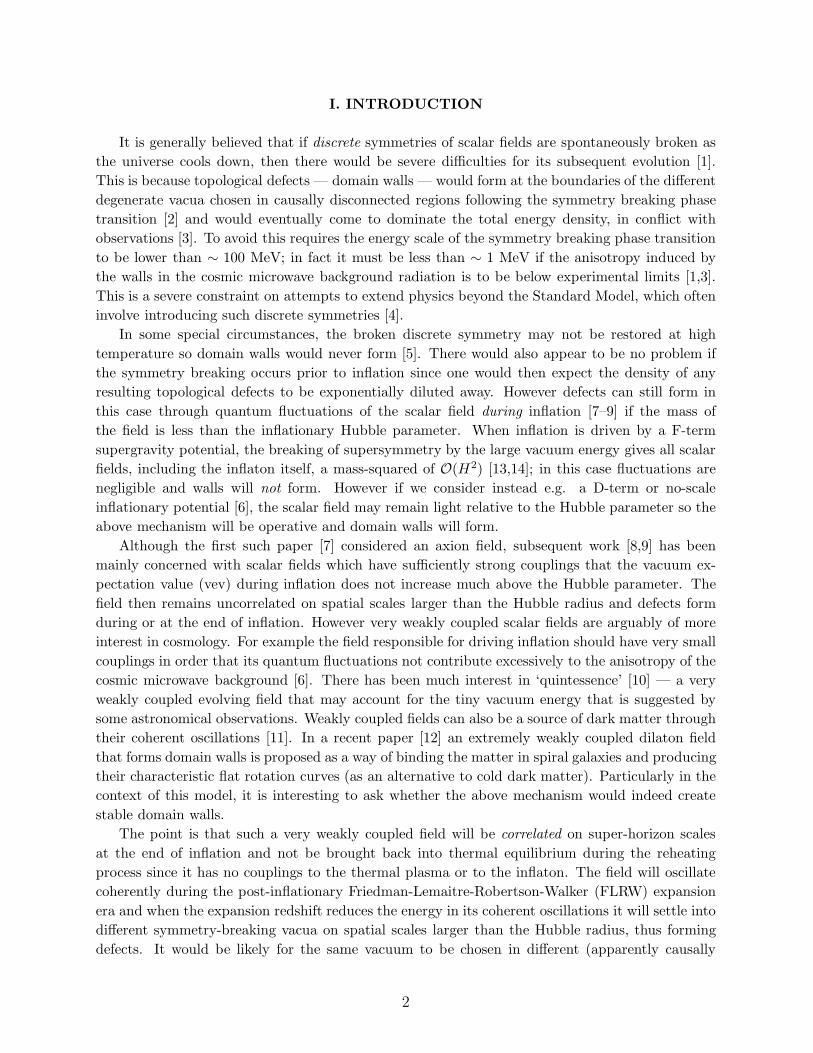
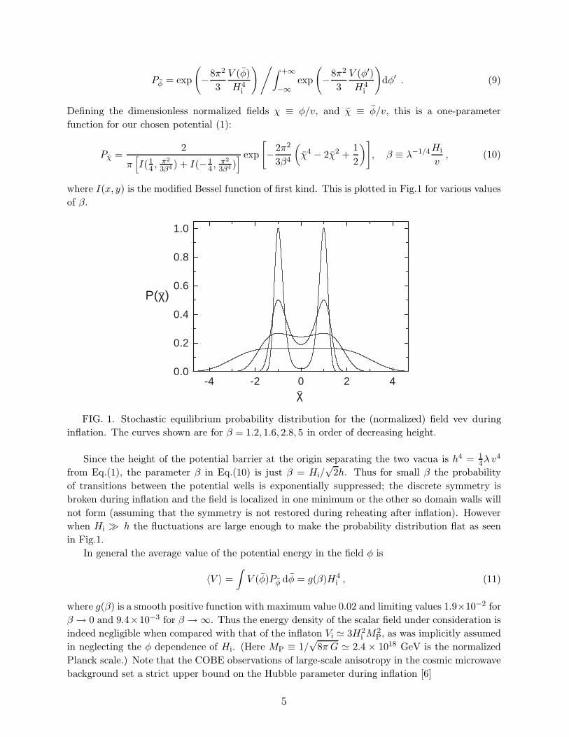
Defining the dimensionless normalized fields χ ≡ φ/v, and χ ≡ φ/v, this is a one-parameter

function for our chosen potential (1):

Pχ =2

π[

I(14 , π2

3β4 ) + I(−14 , π2

3β4 )] exp

[

−2π2

3β4

(

χ4 − 2χ2 +1

2

)

]

, β ≡ λ−1/4 Hi

v, (10)

where I(x, y) is the modified Bessel function of first kind. This is plotted in Fig.1 for various values

of β.

-4 -2 0 2 40.0

0.2

0.4

0.6

0.8

1.0

χ

P(χ)_

_

FIG. 1. Stochastic equilibrium probability distribution for the (normalized) field vev during

inflation. The curves shown are for β = 1.2, 1.6, 2.8, 5 in order of decreasing height.

Since the height of the potential barrier at the origin separating the two vacua is h4 = 14λ v4

from Eq.(1), the parameter β in Eq.(10) is just β = Hi/√

2h. Thus for small β the probability

of transitions between the potential wells is exponentially suppressed; the discrete symmetry is

broken during inflation and the field is localized in one minimum or the other so domain walls will

not form (assuming that the symmetry is not restored during reheating after inflation). However

when Hi ≫ h the fluctuations are large enough to make the probability distribution flat as seen

in Fig.1.

In general the average value of the potential energy in the field φ is

〈V 〉 =

∫

V (φ)Pφ dφ = g(β)H4i , (11)

where g(β) is a smooth positive function with maximum value 0.02 and limiting values 1.9×10−2 for

β → 0 and 9.4×10−3 for β → ∞. Thus the energy density of the scalar field under consideration is

indeed negligible when compared with that of the inflaton Vi ≃ 3H2i M2

P, as was implicitly assumed

in neglecting the φ dependence of Hi. (Here MP ≡ 1/√

8π G ≃ 2.4 × 1018 GeV is the normalized

Planck scale.) Note that the COBE observations of large-scale anisotropy in the cosmic microwave

background set a strict upper bound on the Hubble parameter during inflation [6]

5

V1/4i ≪ 0.027MP =⇒ Hi

MP≪ 4.2 × 10−4. (12)

This still allows the energy scale of inflation to be as high as the GUT scale (∼ 1016 GeV) but in

specific models it can be much lower than this, in particular in ‘new’ inflationary models with a

quadratic leading term in the potential [28].

The average value of |φ| is just v for small β, while for large β it is ∼ 0.305Hi/λ1/4. Thus if

λ <∼ 8 × 10−3, the field vev grows above Hi. The number of e-folds of inflation that are necessary

to achieve the stationary distribution in this case must exceed (〈φ〉/δφ)2 ≃ λ−1/2, taking the field

increment per e-fold to be δφ ≃ Hi/2π. Otherwise one cannot predict an unique probability

distribution for the field.

The slow-roll condition φ ≪ 3Hiφ implies |V ′′(φ)| ≪ 9H2i . For the potential (1) and the

distribution (10) this translates into m2 ≪ 92H2

i if the quadratic term in the potential dominates

(small β). When the quartic term dominates (large β) one must require λ <∼ 1. If the slow-roll

conditions are not obeyed, the classical stochastic treatment does not apply and the quantum

creation of particles is exponentially suppressed [23]. For the case under consideration, h ≪ Hi,

the relevant slow-roll condition is λ <∼ 1 and these two conditions together imply m ≪ Hi.

III. THE EVOLUTION DURING THE FLRW ERA

In Ref. [15] it was shown that the probability distribution for the coarse-grained field outside

the horizon during the FLRW era following the inflationary era evolves into a non-Gaussian distri-

bution. We are interested here in obtaining a discrete probability distribution for the two vacua of

the field. We follow the evolution of the field from its initial value φo at the end of inflation until

it settles down into one of its discrete minima. By obtaining the distribution function f(φo) whose

values are ±1 according to the vacuum finally chosen, we can compute the bias between the vacua.

The equation of motion for the modes of a scalar field outside the horizon during the FLRW

era is

d2φ

dt2+ 3

c

t

dφ

dt+ V ′ = 0 , where c = Ht . (13)

We have rewritten the Hubble parameter in terms of the variable c which equals 1/2 (2/3) for a

radiation- (matter-) dominated universe. The initial conditions are c/t0 = Hi, φ = φo, and φ0 = 0.

In general there is no exact solution for this equation, however a good approximation may easily

be obtained [27].

Let us first suppose that the friction term is relatively unimportant so at first approximation

the field oscillates in its potential minimum at the end of inflation according to the Lagrangian

L = 12 φ2 − V . Then energy conservation implies

φ2 = 2(Vmax − V ) , (14)

where Vmax is the maximum value of the potential energy during the oscillation. Thus the oscillation

period is given (for a symmetric potential) by

∆t = 4

∫ φmax

0

dφ√

2(Vmax − V ). (15)

6

When H ≪ ω = 2π/∆ t the friction term in Eq.(13) is ω/H times smaller than the other terms so

the assumption of negligible friction is valid. Until H drops below ω the field remains approximately

fixed since the friction is relatively high and the dynamical time exceeds the expansion age H−1.

After this point the field starts oscillating, losing energy density of order

∆ρ =

∮

3Hφ dφ = 12H

∫ φmax

0

√

2(Vmax − V )dφ (16)

in each oscillation. Here we have used the fact that in this regime H is approximately constant

during each oscillation period.

For future use we also consider the case of a general power law potential

V (φ) =λ

γφγ . (17)

Let φn be the values of φ that are turning points of the trajectory, tn the corresponding times and

ρn the corresponding energy densities. Evidently φn → 0 and tn grows, eventually going to infinity.

Equations (15) and (16) imply the following relations between these quantities

∆φn =∆ρn

λφγ−1n

= −k2

tnφ2−γ/2

n , (18)

∆tn = k1φ1−γ/2n , (19)

where k1 =(

2√

2πγ Γ(1+1/γ)Γ(1/2+1/γ)

)

λ−1/2 and k2 = c(

12√

2π Γ(1/γ)√γ(2+γ)Γ(1/2+1/γ)

)

λ−1/2. The solution to these

recurrence relations are the power-laws:

φn = φ1na, a = − 6c

2(1 + 3c) + γ(1 − 3c), (20)

tn = t1nb, b =

(2 + γ)

2(1 + 3c) + γ(1 − 3c).

The energy density is ρφ ∼ φγ ∼ taγ/b. In terms of the cosmological scale-factor R this can be

written, ρφ ∼ Raγ/bc, i.e.

ρφ ∼ R−6γ/(2+γ) , (21)

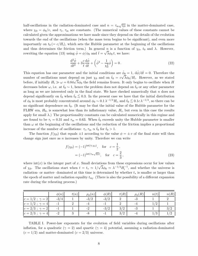
independently of c [27]. The number of oscillations goes as n ∼ φ1/a ∼ t1/b ∼ R1/cb. Table I

shows the exponents of different quantities as functions of n, R and t for the cases of radiation-

and matter- domination and for quadratic and quartic potentials.

Let us return to the double well potential (1) which interests us here. As we saw in the preceding

Section, the quartic term dominates at the end of inflation in the cases of interest, i.e β ≫ 1. The

subsequent evolution starting with φ = φ0 at t = t0 goes as follows. The field oscillates in the

quartic term-dominated potential (where the mass term can be neglected), decreasing in amplitude

due to friction caused by the Hubble expansion, until V 1/4 drops below the height of the barrier h

separating the two vacua, or in other words φ becomes of O(v), and the field settles down in one of

its potential minima. The energy density in oscillations then decreases as for radiation (ρφ ∼ R−4)

independently of the rate of expansion. The relation between the number of half-oscillations and

the field amplitude is n ∼ φ−1 if the universe is radiation-dominated and n ∼ φ−1/2 if it is matter-

dominated. Thus φ will be found around one of its vevs ± v after having completed n = τrχ0

7

half-oscillations in the radiation-dominated case and n = τm√

χ0 in the matter-dominated case,

where χ0 = φ0/v, and τr, τm are constants. (The numerical values of these constants cannot be

calculated given the approximations we have made since they depend on the details of the evolution

towards the end of the oscillations (when the mass term begins to be significant), and even more

importantly on t0 (= c/Hi), which sets the Hubble parameter at the beginning of the oscillations

and thus determines the friction term.) In general n is a function of χ0, t0 and λ. However,

rewriting the equation (13) using φ = φ/φ0 and t =√

λφ0 t, we have:

d2φ

dt2+ 3

c

t

dφ

dt+

(

φ3 − 1

χ20

φ

)

= 0 . (22)

This equation has one parameter and the initial conditions are φ0 = 1, dφ/dt = 0. Therefore the

number of oscillations must depend on just χ0 and on t0 = c√

λφ0/Hi. However, as we stated

before, if initially Hi ≫ ω = 0.84√

λφ0 the field remains frozen. It only begins to oscillate when H

decreases below ω, i.e. at t0 ∼ 1, hence the problem does not depend on t0 or any other parameter

as long as we are interested only in the final state. We have checked numerically that n does not

depend significantly on t0 when t0 <∼ 0.3. In the present case we have that the initial distribution

of φ0 is most probably concentrated around φ0 ∼ 0.1λ−1/4Hi, and t0 <∼ 0.1c λ−1/4, so there can be

no significant dependence on t0. (It may be that the initial value of the Hubble parameter for the

FLRW era, H0, is somewhat less than its inflationary value, Hi, but even in this case the results

apply for small λ.) The proportionality constants can be calculated numerically in this regime and

are found to be τr = 0.31 and τm = 0.63. When t0 exceeds unity the Hubble parameter is smaller

than ω at the beginning of the oscillations and the reduction of the friction implies a proportional

increase of the number of oscillations: τr, τm ∝ t0 for t0 > 1.

The function f(χ0) that equals ±1 according to the value φ = ± v of the final state will then

change sign just once as n increases by unity. Therefore we can write

f(χ0) = (−1)int(τrχ0), for c =1

2,

= (−1)int(τm√

χ0), for c =2

3, (23)

where int(x) is the integer part of x. Small deviations from these expressions occur for low values

of χ0. The oscillations start when t = t∗ ≃ 1/√

λφ0 ≃ λ−1/4H−1i , and whether the universe is

radiation- or matter- dominated at this time is determined by whether t∗ is smaller or larger than

the epoch of matter and radiation equality teq. (There is also the possibility of a different expansion

rate during the reheating process.)

φ(n) t(n) ρφ(n) φ(R) t(R) ρφ(R) n(t) n(R)

c = 1/2 ; γ = 2 -3/4 1 -3/2 -3/2 2 -3 1 2

c = 1/2 ; γ = 4 -1 2 -4 -1 2 -4 1/2 1

c = 2/3 ; γ = 2 -1 1 -2 -3/2 3/2 -3 1 3/2

c = 2/3 ; γ = 4 -2 3 -8 -1 3/2 -4 1/3 1/2

TABLE I. Power-law exponents for the evolution of field variables during oscillations after

inflation, for a quadratic (γ = 2) and quartic (γ = 4) potential, assuming a radiation-dominated

(c = 1/2) and matter-dominated (c = 2/3) universe.

8

Note that the functions (23) apply only when the oscillations begin and end during a period

of expansion while c is constant. As an example of a more complex situation consider the case

where the oscillations start in the radiation-dominated era and end in the matter-dominated one.

According to Table I the amplitude of the oscillations goes as φ ∼ 1/R. The amplitude at the

time of matter-radiation equality is then φeq = φ0(t∗/teq)1/2 ∼ (φ0/teq√

λ)1/2, while the condition

that the oscillations end in the matter-dominated period is φeq > v. The number of oscillations

in the radiation-dominated period is just nr ≃ φ0/φeq = (teq√

λφ0)1/2. Therefore the number of

half-oscillations completed in the radiation-dominated period is proportional to√

φ0. With respect

to the remaining oscillations that occur in the matter-dominated period, since they start at teqwell inside the low friction regime, the constant τm in Eq.(23) has to be scaled by teq =

√λφeqteq.

Accordingly, the matter-dominated period gives the number of oscillations nm ≃√

λφeqteq√

χeq =

λ1/8t1/4eq φ

3/40 /

√v. Thus, for such mixed situations, different functional dependencies of φ0 are

expected in the formula for the number of oscillations.

IV. BIAS

The bias, defined as the difference in the probabilities of populating the two discrete vacua, is

given by the convolution

b(χ) =

∫

f(χ0)Pχ(χ0, χ) dχ0 . (24)

The probability distribution of the field values at the end of inflation Pχ(χ0, χ) is given by Eq.(6)

(rewritten in terms of the normalized fields χ = φ/v and χ = φ/v), while the function f(χ0) that

gives the sign of the field in the final vacuum state was obtained in the previous Section for different

cosmological situations. (Note that Pχ(χ0, χ) is almost independent of spatial scale in the FLRW

era since observable scales correspond to only a few e-foldings during inflation.) In the following

we do a detailed analysis of the bias function for the cases of radiation- and matter-dominated

universes and then present an approximation suitable for more complicated situations.

The bias in the observable universe is well defined by Eq.(24) but since only the probabilistic

distribution (10) is available for χ, the predictions are also in terms of a probability distribution

for the bias which satisfies

Pb =∑

Pχdχ

db, (25)

where χ is understood as a function of b (inverse of the function (24)), and the sum is over the

different branches in the solution of the equation b = b(χ). The cumulative probability for the bias

to be less than some particular value is then just the integral:

P (|b| < x) =∑

∫ b(χ)=x

b(χ)=−xPχ dχ . (26)

The problem has basically two parameters,

α =σ

v∼ Hi

v, (27)

which gives the width of the Gaussian probability distribution (6) in terms of the normalized field

χ0 ≡ φ0/v, and β ∼ λ−1/4α (using Eq.(10)) which gives the width of the distribution (10) of the

9

normalized average field χ ≡ φ/v. The conditions we are assuming for slow-roll m <∼ Hi and λ < 1

imply that α < min(β, β2) but they do not constrain this parameter to be greater or smaller than

unity since we also require β ≫ 1 (i.e. Hi ≫ h) in order for the field to be able to jump the

potential barrier during inflation.

1. Radiation dominated universe

In this case the number of half-oscillations n ∼ τr χ0, and f(χ0) = (−1)int(τr χ0) is a square-

wave. It is easy to see that the bias is then a periodic function of χ with period 2τ−1r , and can be

expanded in the Fourier series

b(χ) =4

π

∞∑

n=0

sin[(2n + 1)πτrχ]

(2n + 1)exp

[

−(2n + 1)πτr√

2α

]2

, (28)

which converges exponentially fast. For α >∼ 1 (i.e. Hi>∼ v) we can approximate the series by its

first term

b(χ) =4

πsin(πτrχ) exp

(

−πτr√2α

)2

, (29)

showing that the bias is a sine function with an exponentially damped amplitude. In the opposite

case α ≪ 1 (i.e. Hi ≪ v), more terms of the series must be added so it converges to the Fourier

series for the square wave, i.e. identical to Eq.(28) without the exponential factor. In this limit

the Gaussian distribution Pχ(χ0, χ) is appropriate inside the regions where f(χ0) has one sign or

the other, but moving χ from one of these regions to another where f(χ0) has opposite sign causes

the function b(χ) to step as the error function, erf(x) ≡ 2√π

∫ x0 dt e−x2

. Therefore for α ≪ 1 we

can write the periodic function b in the interval [−τ−1r , τ−1

r ] as

b(χ) = erf

(

1√2

χ

α

)

− erf

[

1√2

(χ + τ−1r )

α

]

− erf

[

1√2

(χ − τ−1r )

α

]

. (30)

This function is very close to +1 or -1 except in the neighborhood of the origin (or the points nτ−1r )

where it is linearly dependent on χ:

b(χ) =

√

2

π

χ

α, χ < α . (31)

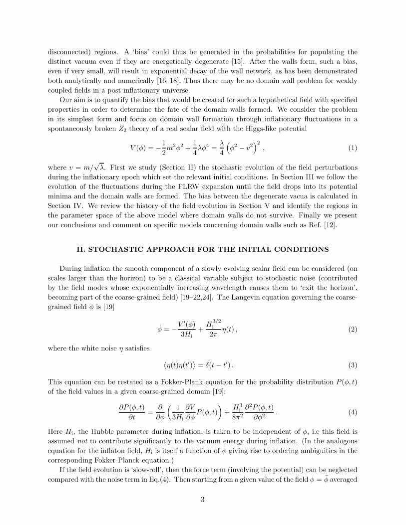
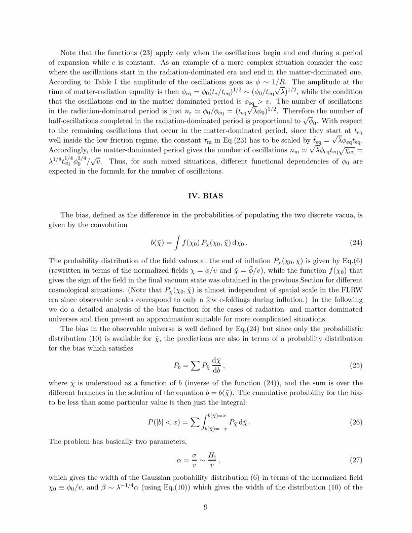
In Fig. 2(a) we show the bias function for several values of α.

When β ≫ 1, we have that φ0 ∼ λ−1/4Hi ≫ v, and the initial values of χ will be distributed

with equal probability in the interval [−τ−1r , τ−1

r ]. Thus, in this case there is no dependence on

β, and the results are relatively insensitive to the initial probability distribution for χ, even if

stochastic equilibrium is not achieved during inflation. Therefore, the bias probability function

P (b) can be simply calculated using Pb(b) = τr2

dχd b with χ in the interval [0, τ−1

r /2], yielding

Pb =1

π

[

(

4

π

)2

exp (−πτrα)2 − b2

]−1/2

for α >∼ 1 , |b| <4

πexp

(

−πτr√2α

)2

,

=

√

π

8τrα for α ≪ 1 , |b| <∼ 1 , (32)

10

-1.5 -1.0 -0.5 0.0 0.5 1.0 1.5

-1.0

-0.5

0.0

0.5

1.0

b(χ)

χ

-6x103

-4x103

-2x103 0 2x10

34x10

36x10

3

-1.0

-0.5

0.0

0.5

1.0

(b)(a)

χ_ _

_

FIG. 2. The bias function for different values of α in (a) the radiation-dominated and (b) the

matter-dominated case. In the left panel, the curves correspond, from top to bottom, to the values

α = 0.05, 0.1, 0.2, 0.4, 0.6, 0.8, while on the right, the bias is shown for α = 100.

where we have shown the maximum value the bias can reach (see Fig.3(a)). The cumulative

probability for the bias is P (|b| < x) = 2τrχ(x), where the function χ(x) is just the inverse of the

bias function in the interval [0, τ−1r /2]. This gives the approximate answer

P (|b| < x) =2

πarcsin

[

πx

4exp

(

πτr√2α

)2]

for x <4

πexp

(

−πτr√2α

)2

, α >∼ 1 ,

=√

2πτrα x for x <∼ 1, α ≪ 1 . (33)

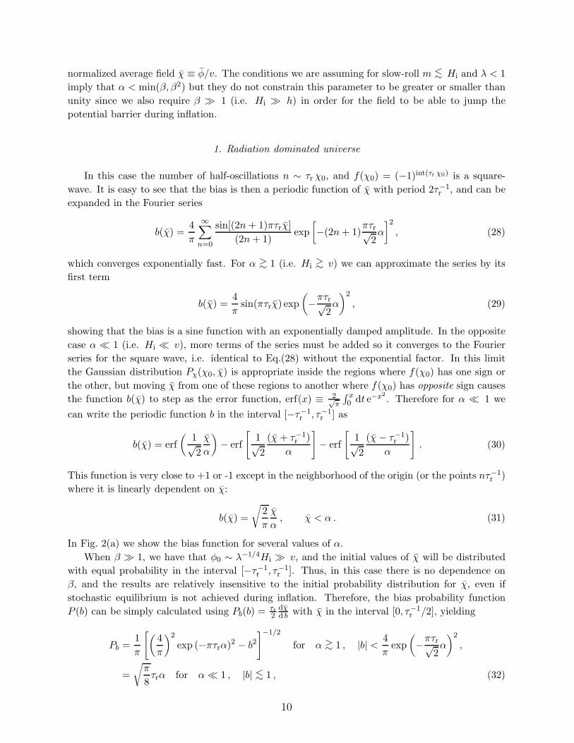
This is plotted in Fig. 3(a) for various values of α.

2. Matter dominated universe

For the matter-dominated universe we have n = τm√

χ0, and the bias will not be a periodic

function of χ. Consequently the bias probability function is more sensitive to the initial probability

distribution of χ, in contrast to the radiation-dominated case. Taking the stochastic distribution

as the initial probability distribution for χ the problem has two parameters rather than just one

as in the radiation-dominated case.

Of course, the bias function b(χ) depends only on α. If α ≪ 1 then the bias will be concentrated

around ±1 since the width of the distribution will not allow different final vacuum states to be

reached. The function will be ±1 except near the transition points χn = τ−2m n2, where it jumps as

±erf( χ−χn√2α

). In fact this will also be the case for values of χ greater than α2 (with α >∼ 1), because

at this point the spacing of χ0 which results in different final states is >∼ α. In the opposite case,

χ <∼ α2, significant cancellation take place and the bias will be reduced. An excellent approximation

in this regime (if α >∼ 1) is given by the formula (29), if we allow for variations in the period and

the amplitude of the sine function according to the effective variation of α with χ (taking into

account the increasing distance between the χn with n in the matter dominated case), i.e.

11

0.0 0.2 0.4 0.6 0.8 1.00.0

0.2

0.4

0.6

0.8

1.0

(b)(a)

P(b<x)

x

0.0 0.2 0.4 0.6 0.8 1.00.0

0.2

0.4

0.6

0.8

1.0

x

FIG. 3. The cumulative probability in (a) the radiation-dominated and (b) the mat-

ter-dominated case. In the left panel, the curves correspond, from bottom to top, to the values

α = 0.05, 0.1, 0.2, 0.4, 0.6, 0.8 (as in Fig. 2(a)), while in the right panel the curves correspond, from

bottom to top, to the values α/√

β = 0.2, 0.45, 0.7, 1.0, 1.6, 2.2, 3.2.

b(χ) =4

πsgn(χ) exp

[

− 1

|χ|

(

πτmα

2√

2

)2]

sin

(

πτm

√

|χ|)

, for χ <∼ α2 . (34)

In Fig. 2(b) we show an example of the bias function for the matter-dominated case.

For the case of interest, i.e. β ≫ 1, the mass term can be neglected in Eq.(10) and the initial

probability for χ writes

Pχ =

√π

23/431/4Γ(5/4)βexp

(

−2π2

3β−4χ4

)

. (35)

This function is practically constant for χ < β/2 and then falls until χ = β where it is nearly zero.

Thus for β ≫ α2 the bias is ±1 with high probability because χ ∼ β. In this case we recover the

linear behavior (33) of the cumulative probability for the bias in the radiation-dominated case, but

now the spacing τ−1r depends on β:

P (|b| < x) =√

2πα

0.71√

βx , for x <∼ 1, α ≪

√

β , (36)

where the precise coefficient in the identification τ−1r ∼ √

β is 25/8Γ(9/8)√5Γ(5/4)

≃ 0.71, as can be calculated

from the average value of the inverse spacing.

For α < β <∼ α2 the bias has higher probability between −1 and 1. In this case the probability

P (|b| < x) is dominated by the sector in the bias function (34) where x > 4π exp

[

− 1|χ|

(

πτmα2√

2

)2]

and thus |χ| < χx = −(πτmα2√

2)2/ log(π

4 x). Then

P (|b| < x) = 2

∫ χx

0Pχ dχ = 1 − Γ(1

4 , β−4χ4x)

Γ(14 )

, for√

β <∼ α , (37)

12

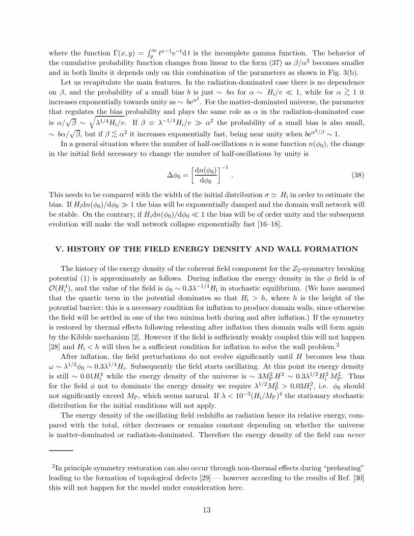
where the function Γ(x, y) =∫∞y tx−1e−td t is the incomplete gamma function. The behavior of

the cumulative probability function changes from linear to the form (37) as β/α2 becomes smaller

and in both limits it depends only on this combination of the parameters as shown in Fig. 3(b).

Let us recapitulate the main features. In the radiation-dominated case there is no dependence

on β, and the probability of a small bias b is just ∼ bα for α ∼ Hi/v ≪ 1, while for α >∼ 1 it

increases exponentially towards unity as ∼ beα2

. For the matter-dominated universe, the parameter

that regulates the bias probability and plays the same role as α in the radiation-dominated case

is α/√

β ∼√

λ1/4Hi/v. If β ≡ λ−1/4Hi/v ≫ α2 the probability of a small bias is also small,

∼ bα/√

β, but if β <∼ α2 it increases exponentially fast, being near unity when beα2/β ∼ 1.

In a general situation where the number of half-oscillations n is some function n(φ0), the change

in the initial field necessary to change the number of half-oscillations by unity is

∆φ0 =

[

dn(φ0)

dφ0

]−1

. (38)

This needs to be compared with the width of the initial distribution σ ≃ Hi in order to estimate the

bias. If Hidn(φ0)/dφ0 ≫ 1 the bias will be exponentially damped and the domain wall network will

be stable. On the contrary, if Hidn(φ0)/dφ0 ≪ 1 the bias will be of order unity and the subsequent

evolution will make the wall network collapse exponentially fast [16–18].

V. HISTORY OF THE FIELD ENERGY DENSITY AND WALL FORMATION

The history of the energy density of the coherent field component for the Z2-symmetry breaking

potential (1) is approximately as follows. During inflation the energy density in the φ field is of

O(H4i ), and the value of the field is φ0 ∼ 0.3λ−1/4Hi in stochastic equilibrium. (We have assumed

that the quartic term in the potential dominates so that Hi > h, where h is the height of the

potential barrier; this is a necessary condition for inflation to produce domain walls, since otherwise

the field will be settled in one of the two minima both during and after inflation.) If the symmetry

is restored by thermal effects following reheating after inflation then domain walls will form again

by the Kibble mechanism [2]. However if the field is sufficiently weakly coupled this will not happen

[28] and Hi < h will then be a sufficient condition for inflation to solve the wall problem.2

After inflation, the field perturbations do not evolve significantly until H becomes less than

ω ∼ λ1/2φ0 ∼ 0.3λ1/4Hi. Subsequently the field starts oscillating. At this point its energy density

is still ∼ 0.01H4i while the energy density of the universe is ∼ 3M2

P H2 ∼ 0.3λ1/2H2i M2

P. Thus

for the field φ not to dominate the energy density we require λ1/2M2P > 0.03H2

i , i.e. φ0 should

not significantly exceed MP, which seems natural. If λ < 10−3(Hi/MP)4 the stationary stochastic

distribution for the initial conditions will not apply.

The energy density of the oscillating field redshifts as radiation hence its relative energy, com-

pared with the total, either decreases or remains constant depending on whether the universe

is matter-dominated or radiation-dominated. Therefore the energy density of the field can never

2In principle symmetry restoration can also occur through non-thermal effects during “preheating”

leading to the formation of topological defects [29] — however according to the results of Ref. [30]

this will not happen for the model under consideration here.

13

dominate since it did not do so initially when the field was began to oscillate at the end of inflation.

However after the domain walls form, the relative energy density starts increasing again (at least

until the wall network decays due to the bias). The field is released when t = t∗ ∼ (λ1/4Hi)−1 and

subsequently its energy density decays as ρφ = (R∗/R)4H4i . The walls will form when ρφ decreases

below h4 i.e. at a time tw determined by

R(tw)

R(t∗)∼ Hi

h. (39)

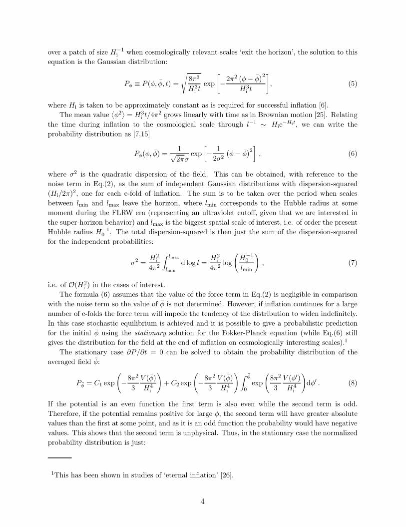
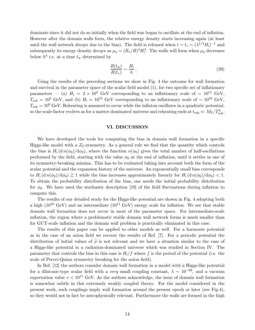
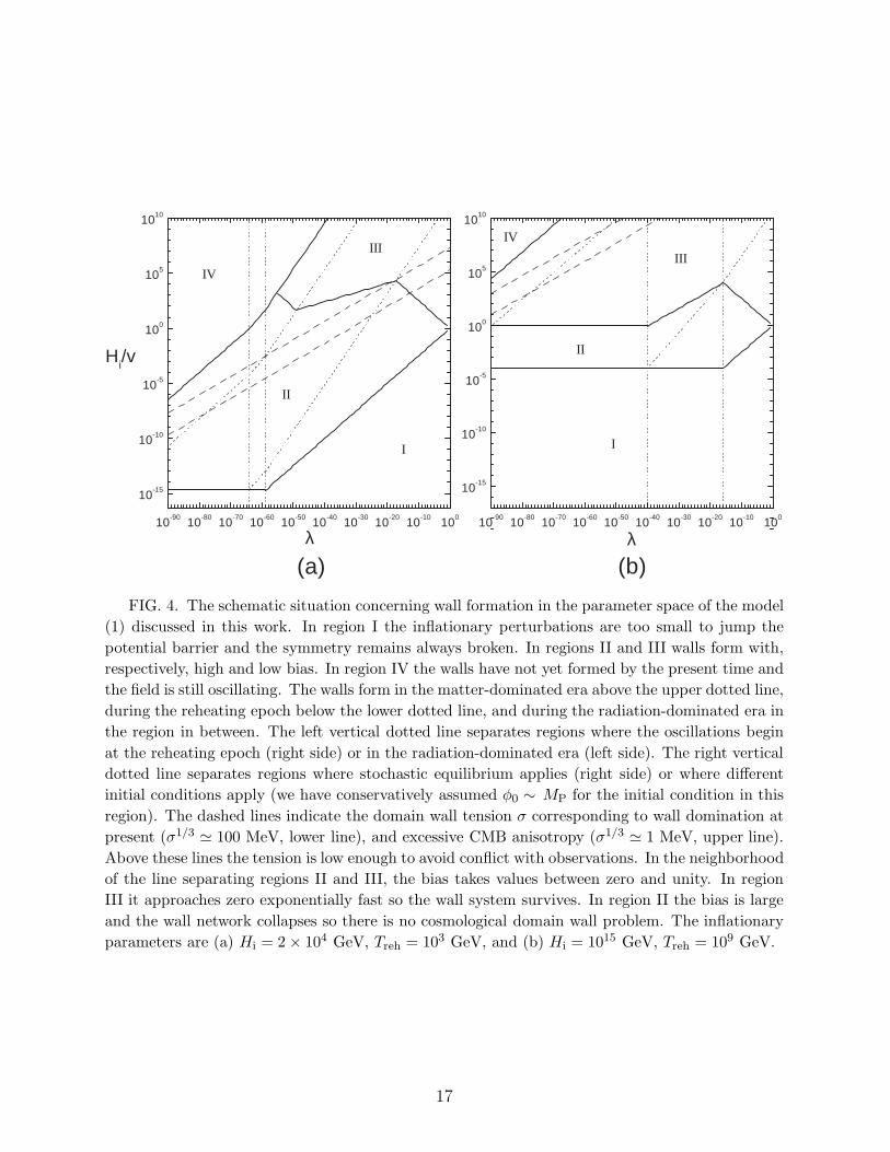
Using the results of the preceding sections we show in Fig. 4 the outcome for wall formation

and survival in the parameter space of the scalar field model (1), for two specific set of inflationary

parameters — (a) Hi = 2 × 104 GeV corresponding to an inflationary scale of ∼ 1011 GeV,

Treh = 103 GeV, and (b) Hi = 1015 GeV corresponding to an inflationary scale of ∼ 1016 GeV,

Treh = 109 GeV. Reheating is assumed to occur while the inflaton oscillates in a quadratic potential,

so the scale-factor evolves as for a matter-dominated universe and reheating ends at treh ≃ MP/T 2reh.

VI. DISCUSSION

We have developed the tools for computing the bias in domain wall formation in a specific

Higgs-like model with a Z2-symmetry. As a general rule we find that the quantity which controls

the bias is Hi (d n(φ0)/dφ0), where the function n(φ0) gives the total number of half-oscillations

performed by the field, starting with the value φ0 at the end of inflation, until it settles in one of

its symmetry-breaking minima. This has to be evaluated taking into account both the form of the

scalar potential and the expansion history of the universe. An exponentially small bias corresponds

to Hi (d n(φ0)/dφ0) >∼ 1 while the bias increases approximately linearly for Hi (d n(φ0)/dφ0) < 1.

To obtain the probability distribution of the bias, one needs the initial probability distribution

for φ0. We have used the stochastic description [19] of the field fluctuations during inflation to

compute this.

The results of our detailed study for the Higgs-like potential are shown in Fig. 4 adopting both

a high (1016 GeV) and an intermediate (1011 GeV) energy scale for inflation. We see that stable

domain wall formation does not occur in most of the parameter space. For intermediate-scale

inflation, the region where a problematic stable domain wall network forms is much smaller than

for GUT-scale inflation and the domain wall problem is practically eliminated in this case.

The results of this paper can be applied to other models as well. For a harmonic potential

as in the case of an axion field we recover the results of Ref. [7]. For a periodic potential the

distribution of initial values of φ is not relevant and we have a situation similar to the case of

a Higgs-like potential in a radiation-dominated universe which was studied in Section IV. The

parameter that controls the bias in this case is Hi/f where f is the period of the potential (i.e. the

scale of Peccei-Quinn symmetry breaking for the axion field).

In Ref. [12] the authors consider domain wall formation in a model with a Higgs-like potential

for a dilatonic-type scalar field with a very small coupling constant, λ ∼ 10−88, and a vacuum

expectation value v < 1011 GeV. As the authors acknowledge, the issue of domain wall formation

is somewhat subtle in this extremely weakly coupled theory. For the model considered in the

present work, such couplings imply wall formation around the present epoch or later (see Fig.4),

so they would not in fact be astrophysically relevant. Furthermore the walls are formed in the high

14

bias region unless Hi>∼ 1013 GeV. However unlike the model considered in this work, the dilatonic

field of Ref. [12] also couples universally with matter through the term

Lint = exp

(

φ

M∗

)

θµµ, (40)

where θµµ is the trace of the energy-momentum tensor and M∗2 >∼ (103 − 104)M2

P. During inflation

the trace θµµ is non-zero, driving the field quickly to large negative values φ <∼ −70M∗ (where the

exponential factor in Eq.(40) makes the size of this interaction term comparable to the Higgs-like

potential). Thus the effective mass is much smaller than Hi and the generation of fluctuations of

size Hi is unavoidable. After inflation the term (40) decreases rapidly, so the field must relax in

the quartic potential alone, starting at scales higher than the Planck mass. As we have previously

discussed the absence of a force term strong enough to drive the field to the origin will make

the potential energy of the field dominate the energy density of the universe. In Ref. [12] the

authors also introduce a term that couples the field coherently to the thermal bath during the

radiation-dominated era,

Vtherm =κ

2H2φ2 ∼ T 4

M2P

φ2 , (41)

where κ is a numerical constant. The intention in doing so is to drive the field to the origin,

restoring the symmetry, so domain walls would be formed when H falls below the (vacuum) mass

of the field. However, if φ is initially greater than the Planck mass this term will exceed the energy

density of the universe so the treatment is not consistent. This problem does not occur if κ ≪ 1

but in that case the mass of the field is always much smaller than H so the thermal term cannot

affect the field.

Apart from this problem with the initial conditions, it is interesting to examine the effect of the

coupling (41) with the thermal bath on the damping of the oscillations. The equation of motion

for the field in the radiation-dominated universe with such a potential term is exactly solvable,

with the general solution

φ(t) = c1t−(1+

√1−4κ)/4 + c2t

−(1−√

1−4κ)/4. (42)

For κ ≪ 1/4 the friction dominates and the field decreases very slowly as t−κ/2 (dominant term

in Eq.(42)), while for κ > 1/4 the behavior is oscillatory and the amplitude decreases as t−1/4 ∼R−1/2. Thus in either case the field amplitude decreases more slowly than for the quartic potential

we have considered, where φ ∼ R−1, or even for the quadratic potential, where φ ∼ R−3/2. This

makes it even more unlikely that the walls can be formed before the present epoch. Thus this

interesting attempt to do away with dark matter in galaxies by modifying the gravitational force

law cannot work.

ACKNOWLEDGMENTS

We would like to thank Graham Ross for helpful comments and encouragement. HC was

supported by a CONICET Fellowship (Argentina).

15

REFERENCES

[1] Ya.B. Zel’dovich, I.Y. Kobzarev and L.B. Okun, Sov. Phys. JETP 40, 1 (1975).

[2] T.W.B. Kibble, J. Phys. A9, 1387 (1976).

[3] For a review, see, A. Vilenkin and E.P.S. Shellard, Cosmic Strings and Other Topological

Defects (Cambridge University Press, 1994).

[4] For reviews, see, R.D. Peccei, in Broken Symmetries, Lecture Notes in Physics, Vol. 521, edited

by L. Mathelitsch and W. Plessas (Springer, 1999) p.299; L. Wolfenstein, in Fundamental

Symmetries In Nuclei And Particles, edited by H. Henrikson and P. Vogel (World Scientific,

1990) p.183.

[5] G. Dvali and G. Senjanovic, Phys. Rev. Lett. 74, 5178 (1995); B. Bajc, A. Riotto and G.

Senjanovic, Phys. Rev. Lett. 81, 1355 (1998).

[6] D.H. Lyth and A. Riotto, Phys. Rept. 314, 1 (1999).

[7] A.D. Linde and D.H. Lyth, Phys. Lett. B246, 353 (1990).

[8] H.M. Hodges and J.R. Primack, Phys. Rev. D43, 3155 (1991).

[9] M. Nagasawa and J. Yokoyama, Nucl. Phys. B370, 472 (1992).

[10] For a review, see, P. Binetruy, Int. J. Theor. Phys. 39, 1859 (2000).

[11] See, e.g., P.J.E. Peebles, Astrophys. J. 534, L27 (2000); J. Goodman, New Astron. 5, 103

(2000).

[12] G. Dvali, G. Gabadadze and M. Shifman, Mod. Phys. Lett. A16, 513 (2001).

[13] M. Dine, W. Fischler and D. Nemechansky, Phys. Lett. B136, 169 (1984).

[14] G. Coughlan, W. Fischler, E.W. Kolb, S. Raby and G.G. Ross, Phys. Lett. 140B (1984) 44.

[15] Z. Lalak, S. Thomas and B. Ovrut, Phys. Lett. B306, 10 (1993).

[16] D. Coulson, Z. Lalak and B. Ovrut, Phys. Rev. D53, 4237 (1996).

[17] M. Hindmarsh, Phys. Rev. Lett. 77, 4495 (1996).

[18] S. E. Larsson, S. Sarkar and P. White, Phys. Rev. D55, 5129 (1997).

[19] A.A. Starobinsky, in Current Topics in Field Theory, Quantum Gravity and Strings, edited

by H.J. de Vega and N. Sanchez (Springer, 1986) p.107.

[20] A. Goncharov and A. Linde, Sov. J. Part. Nucl. 17, 369 (1986).

[21] S.J. Rey, Nucl. Phys. B284, 706 (1987).

[22] M. Sasaki, Y. Nambu and K. Nakao, Nucl. Phys. B308, 868 (1988).

[23] M. Bellini, H. Casini, R. Montemayor and P. Sisterna, Phys. Rev. D54, 7172 (1996).

[24] For a review, see, A. Linde, Particle Physics and Inflationary Cosmology (Harwood Academic,

1990).

[25] A. Vilenkin and L.H. Ford, Phys. Rev. D26, 1231 (1982); A.D. Linde, Phys. Lett. B116, 335

(1982); A.A. Starobinsky, Phys. Lett. B117, 175 (1982).

[26] A. Vilenkin, Phys. Rev. D27, 2848 (1983); A. Linde and A. Mezhlumian, Phys. Lett. B307,

25 (1993).

[27] M.S. Turner, Phys. Rev. D28, 1243 (1983).

[28] G. German, G.G. Ross and S. Sarkar, Nucl. Phys. B608, 423 (2001).

[29] I. Tkachev, S. Khlebnikov, L. Kofman and A. Linde, Phys. Lett. B440, 262 (1998).

[30] P.B. Greene, L. Kofman, A. Linde and A.A. Starobinsky, Phys. Rev. D56, 6175 (1997).

16

10-90 10-80 10-70 10-60 10-50 10-40 10-30 10-20 10-10 100

10-15

10-10

10-5

100

105

1010

λ

Hi/v

IV

III

II

I

10-90

10-80

10-70

10-60

10-50

10-40

10-30

10-20

10-10

100

10-15

10-10

10-5

100

105

1010

(a) (b)λ

IV

III

II

I

FIG. 4. The schematic situation concerning wall formation in the parameter space of the model

(1) discussed in this work. In region I the inflationary perturbations are too small to jump the

potential barrier and the symmetry remains always broken. In regions II and III walls form with,

respectively, high and low bias. In region IV the walls have not yet formed by the present time and

the field is still oscillating. The walls form in the matter-dominated era above the upper dotted line,

during the reheating epoch below the lower dotted line, and during the radiation-dominated era in

the region in between. The left vertical dotted line separates regions where the oscillations begin

at the reheating epoch (right side) or in the radiation-dominated era (left side). The right vertical

dotted line separates regions where stochastic equilibrium applies (right side) or where different

initial conditions apply (we have conservatively assumed φ0 ∼ MP for the initial condition in this

region). The dashed lines indicate the domain wall tension σ corresponding to wall domination at

present (σ1/3 ≃ 100 MeV, lower line), and excessive CMB anisotropy (σ1/3 ≃ 1 MeV, upper line).

Above these lines the tension is low enough to avoid conflict with observations. In the neighborhood

of the line separating regions II and III, the bias takes values between zero and unity. In region

III it approaches zero exponentially fast so the wall system survives. In region II the bias is large

and the wall network collapses so there is no cosmological domain wall problem. The inflationary

parameters are (a) Hi = 2 × 104 GeV, Treh = 103 GeV, and (b) Hi = 1015 GeV, Treh = 109 GeV.

17