No Contagion, Only Interdependence: Measuring Stock Market Co-movements

No Contagion, Only Interdependence:

Measuring Stock Market Co-movements1

Kristin Forbes

M.I.T.-Sloan School of Management

Roberto Rigobon

M.I.T.-Sloan School of Management and NBER

First Version: April 1998

This Version: February 2000

1Thanks to Rudiger Dornbusch, Andrew Rose, Jaume Ventura, and seminar participants at M.I.T.,Dartmouth, and N.Y.U. for helpful comments and suggestions. All remaining errors are ours. Com-ments are welcomed to either author: Kristin Forbes at 50 Memorial Drive, Room E52-446, Cambridge,MA 02142; email: [email protected]; home page http://web.mit.edu/kjforbes/www/ and Roberto Rigobonat 50 Memorial Drive, Room E52-447, Cambridge, MA 02142; email: [email protected]; home page:http://web.mit.edu/rigobon/www/.

Abstract

This paper tests for stock market contagion during recent financial crises. It defines contagion as

a significant increase in market co-movement after a shock to one country (or group of countries).

Previous work based on the correlation coefficient has found strong evidence of this type of contagion

during recent financial crises. We show, however, that these tests are biased because the unadjusted

cross-market correlation coefficient is conditional on market volatility. It is possible to correct for

this bias, and when we make this adjustment, there is virtually no evidence of contagion during

the 1997 East Asian crisis, the 1994 Mexican peso collapse, and the 1987 U.S. stock market crash.

There is still a high level of market co-movement during these crisis periods, however, which reflects

a continuation of strong cross-market linkages which exist in all states of the world. In other words,

during these three crises, there was no contagion, only interdependence.

JEL Classification: F30, F40, G15

Keywords: Contagion, Stock Market, Interdependence

Kristin Forbes Roberto RigobonSloan School of Management, MIT Sloan School of Management, MIT50 Memorial Drive, E52-446 50 Memorial Drive, E52-447Cambridge, MA 02142-1347 Cambridge, MA 02142-1347

and [email protected] [email protected]

1 Introduction

In October of 1997, the Hong Kong market plummeted and then partially rebounded. As shown in

Figure 1, these dramatic movements were mirrored in markets in North America, South America,

Europe, and the rest of Asia. In December of 1994, the Mexican market cratered, and as shown in

Figure 2, this plunge was quickly reflected in other major Latin American markets. Figure 3 shows

that in October of 1987 the crash of the US market quickly affected major stock markets around

the globe. These cases show that dramatic movements in one stock market can have a powerful

impact on markets of very different sizes and structures throughout the world. Does this high rate

of stock market co-movement during periods of market turmoil constitute contagion?

Before answering this question, it is necessary to define contagion. There is widespread disagree-

ment about what this term entails, and this paper will utilize the narrow definition of contagion

which has historically been used in this literature. This paper defines contagion as a significant in-

crease in cross-market linkages after a shock to one country (or group of countries.)1 Cross-market

linkages can be measured by a number of different statistics, such as the correlation in asset returns,

the probability of a speculative attack, or the transmission of shocks or volatility. According to this

definition, if two markets show a moderate degree of co-movement during periods of stability, such

as Germany and Italy, and then a shock to one market leads to a significant increase in market

co-movement, this would constitute contagion. On the other hand, if two markets show a high

degree of co-movement during periods of stability, even if they continue to be highly correlated

after a shock to one market, this may not constitute contagion. It is only contagion if cross-market

co-movement increases significantly after the shock. If the co-movement does not increase signif-

icantly, then any continued high level of market co-movement suggests strong linkages between

the two economies which exist in all states of the world. This is what we call interdependence.

Based on this approach, contagion implies that cross-market linkages are fundamentally different

after a shock to one market, while interdependence implies no significant change in cross-market

relationships during a crisis.2

1 In a closely related paper, Forbes and Rigobon (1999) propose using the term “shift-contagion” instead of “con-tagion” in order to clarify exactly what this term entails. The term shift-contagion is sensible because it not onlyclarifies that contagion arises from a shift in cross-market linkages, but it also avoids taking a stance on how thisshift ocurred.

2 It is important to note that this definition of contagion is not universally accepted. Some economists argue that

1

Although this definition of contagion is restrictive, it has two important advantages. First, it

provides a straightforward framework for testing if contagion occurs. Simply compare the correla-

tion (or covariance) between two markets during a relatively stable period (generally measured as a

historic average) with that during a period of turmoil (directly after a shock occurs). Contagion is

a significant increase in the cross-market relationship during the period of turmoil. This simple and

intuitive test for contagion has formed the basis of this literature. A second benefit of this defini-

tion of contagion is that it provides a straightforward method of distinguishing between alternative

explanations of how shocks are transmitted across markets. As discussed in the next section, there

is an extensive theoretical literature on the international propagation of shocks. Many theories as-

sume that investors (or institutions) behave differently after a large negative shock. Other theories

argue that most shocks are propagated through real linkages, such as trade. It is extremely difficult

to measure these various transmission mechanisms directly. By defining contagion as a significant

increase in cross-market linkages, this paper avoids having to directly measure and differentiate

between these various propagation mechanisms. Moreover, tests based on this definition provide

a useful method of classifying theories as those which entail either a change in propagation mech-

anisms after a shock versus those which are a continuation of existing mechanisms. Identifying

if this type of contagion exists could therefore provide evidence for or against certain theories of

transmission.

While contagion can take many forms, this paper focuses on contagion across stock markets. The

first half of the paper discusses conceptual issues involved in measuring this contagion. Section 2

briefly reviews the relevant theoretical and empirical literature. Section 3 discusses the conventional

technique of measuring stock market contagion and proves that the correlation coefficient central

to this analysis is biased. The correlation coefficient is actually conditional on market volatility

over the time period under consideration, so that during a period of turmoil when stock market

volatility increases, unadjusted estimates of cross-market correlations will be biased upward. We

show how to adjust the correlation coefficient to correct for this bias.

The second half of this paper applies these concepts in empirical tests for contagion during

contagion occurs whenever a shock to one country is transmitted to another country, even if there is no significantchange in cross-market relationships. Others argue that it is impossible to define contagion using tests for changesin cross-market linkages. Instead, they argue that it is necessary to identify exactly how a shock is propagated acrosscountries, and only certain types of transmission mechanisms (no matter what the magnitude) constitute contagion.

2

three periods of market turmoil: the 1997 East Asian crisis, the 1994 Mexican peso collapse, and

the 1987 US stock market crash. Sections 4 through 6 test if average cross-market correlations

increase significantly during the relevant period of turmoil. For each of the three crises, tests based

on the unadjusted correlation coefficients suggest that there was contagion in several markets.

When the same tests are based on the adjusted correlation coefficients, however, the incidence

of contagion falls dramatically (to zero in most cases.) This suggests that high cross-market co-

movements during the recent East Asian crisis, the Mexican peso collapse, and the 1987 US market

crash, were a continuation of strong cross-market interdependence instead of contagion. In other

words, many economies are closely linked in all states of the world, and these linkages were not

significantly different during these three crisis periods. The final section of the paper summarizes

these findings and discusses several caveats to these results. It also introduces the new puzzle of

“excess interdependence” found in this paper.

2 The International Propagation of Shocks: Theory and Previous

Evidence

As discussed above and shown in Figures 1-3, stock markets of very different structures, sizes,

and geographic locations can exhibit a high degree of co-movement. Since most country risk

is idiosyncratic, this high degree of co-movement suggests the existence of mechanisms through

which domestic shocks are transmitted internationally. This section begins by summarizing the

theoretical work on international propagation mechanisms. It then proposes a general framework

through which to interpret and measure these mechanisms and discusses the difficulties inherent in

testing these channels. The section closes with a brief review of previous empirical work measuring

stock market co-movements and testing for contagion.

2.1 Propagation Mechanisms: The Theory

The theoretical literature on how shocks are propagated internationally is extensive. Recent work

in this field is well-summarized in Claessens, Dornbusch and Park (1999). For the purpose of this

paper, however, it is useful to divide this broad set of theories into two groups: crisis-contingent and

non-crisis-contingent theories. Crisis-contingent theories are those which explain why transmission

3

20406080100

120

140 09

/01/

9709

/15/

9709

/29/

9710

/13/

9710

/27/

9711

/10/

9711

/24/

9712

/08/

9712

/22/

97

Hon

g Ko

ngIn

done

sia

Kore

aTh

aila

ndBr

azil

Mex

ico

Can

ada

Ger

man

yU

KU

S

Figure 1: 1997 East Asian Crises. Stock Market Indices in US$.

4

405060708090100

110 11

/01/

9411

/11/

9411

/21/

9412

/01/

9412

/11/

9412

/21/

9412

/31/

9401

/10/

9501

/20/

9501

/30/

95

Arge

ntin

aBr

azil

Chi

leM

exic

oC

anad

aG

erm

any

US

Figure 2: 1994 Mexican Peso Collapse. Stock Market Indices in US$.

5

405060708090100

110

120 10

/01/

8710

/15/

8710

/29/

8711

/12/

8711

/26/

8712

/10/

8712

/24/

87H

ong

Kong

Japa

nAu

stra

liaC

anad

aFr

ance

Ger

man

yN

ethe

rland

sSw

itzer

land

UK

US

Figure 3: 1987 U.S. Stock Market Crash. Stock Market Indices in US$.

6

mechanisms change during a crisis and therefore why cross-market linkages increase after a shock.

Non-crisis-contingent theories assume that transmission mechanisms are the same during a crisis

and during more stable periods, and therefore cross-market linkages do not increase after a shock.

Under our definition, contagion is explained by the crisis-contingent theories.

2.2 Crisis-Contingent Theories

Crisis-contingent theories of how shocks are transmitted internationally can be divided into three

mechanisms: multiple equilibria; endogenous liquidity; and political economy. The first mechanism,

multiple equilibria, occurs when a crisis in one country is used as a sunspot for other countries. For

example Masson [1997] shows how a crisis in one country could coordinate investors’ expectations,

shifting them from a good to a bad equilibrium for another economy, and thereby cause a crash

in the second economy. Mullainathan [1998] argues that investors imperfectly recall past events.

A crisis in one country could trigger a memory of past crises, which would cause investors to

recompute their priors (on variables such as debt default) and assign a higher probability to a bad

state. The resulting downward co-movement in prices would occur because memories (instead of

fundamentals) are correlated. In both of these models, the shift from a good to bad equilibrium,

and the transmission of the initial shock, is therefore driven by a change in investor expectations

or beliefs and not by any real linkages. This branch of theories can not only explain the bunching

of crises, but also why speculative attacks occur in economies that appear to be fundamentally

sound.3 These qualify as crisis-contingent theories because the change in the price of the second

market (relative to the change in the price of the first) is exacerbated during the shift between

equilibria. In other words, after the crisis in the first economy, investors change their expectations

and therefore transmit the shock through a propagation mechanism that does not exist during

stable periods.

A second category of crisis-contingent theories is endogenous liquidity shocks. Calvo [1999]

develops a model where there is asymmetric information among investors. Informed investors

receive signals about the fundamentals of a country and are hit by liquidity shocks (margin calls)

which may force them to sell their holdings. Uninformed investors cannot distinguish between a

3This point has been raised by Radelet and Sachs [1998a, 1998b], and Sachs, Tornell and Velasco [1996] for thecase of Hong Kong.

7

liquidity shock and a bad signal, and therefore charge a premium when the informed investors are

net sellers.4 In this model, the liquidity shock increases the correlation in asset prices.5

A final transmission mechanism which can be categorized as a crisis-contingent theory is political

contagion. Drazen [1998] studies the European devaluations in 1992-3 and develops a model which

assumes that central bank presidents are under political pressure to maintain their countries’ fixed

exchange rates. When one country decides to abandon its peg, this reduces the political costs to

other countries of abandoning their respective pegs, which increases the likelihood of these countries

switching exchange rate regimes. As a result, exchange rate crises may be bunched together, and

once again, transmission of the initial shock occurs through a mechanism (political economy) which

did not exist before the initial crisis.

This group of crisis-contingent theories suggests a number of very different channels through

which shocks could be transmitted internationally: multiple equilibria based on investor psychol-

ogy; endogenous-liquidity shocks causing a portfolio recomposition; and political economy affecting

exchange rate regimes. Despite the different approaches and models used to develop these theories,

they all share one critical implication: the transmission mechanism in the period after the initial

crisis is inherently different than that before the shock. The crisis causes a structural shift, so that

shocks are propagated via a channel which does not exist in stable periods. Therefore, each of these

theories could explain the existence of contagion as defined above.

2.3 Non-Crisis-Contingent Theories

On the other hand, the remainder of the theories explaining how shocks could be propagated

internationally would not generate contagion (as defined in this paper) because they would not

generate a change in the propagation mechanism. These theories imply that any large or small

cross-market correlations after a shock are a continuation of linkages which existed before the

crisis. These channels are often called “real linkages” since many (although not all) are based on

economic fundamentals. These theories can be divided into four broad channels: trade; policy

coordination; country reevaluation; and random aggregate shocks.

4See also Yuan [2000] for a formal solution to this problem.5This endogenous liquidity shock is fundamentally different than an exogenous liquidity shock (which is discussed

in the next section.) An endogenous liquidity shock generates a change in the propagation mechanism, while anexogenous liquidity shock does not.

8

The first transmission mechanism, trade, could work through several related effects.6 If one

country devalues its currency, this would have the direct effect of increasing the competitiveness

of that country’s goods, potentially increasing exports to a second country and hurting domestic

sales within the second country. The initial devaluation could also have the indirect effect of

reducing export sales from other countries which compete in the same third market. Either of

these effects could not only have a direct impact on a country’s sales and output, but if the loss

in competitiveness is severe enough, it could increase expectations of an exchange rate devaluation

and/or lead to an attack on a country’s currency.

The second transmission mechanism, policy coordination, links economies because one country’s

response to an economic shock could force another country to follow similar policies. For example,

a trade agreement might include a clause in which lax monetary policy in one country forces other

member countries to raise trade barriers.

The third propagation mechanism, country reevaluation or learning (which includes models of

herding and informational cascades), argues that investors may apply the lessons learned after a

shock in one country to other countries with similar macroeconomic structures and policies.7 For

example, if a country with a weak banking system is discovered to be susceptible to a currency

crisis, investors could reevaluate the strength of the banking system in other countries and adjust

their expected probabilities of a crisis accordingly.

The final non-crisis-contingent transmission mechanism are random aggregate or global shocks

which simultaneously affect the fundamentals of several economies. For example, a rise in the

international interest rate, a contraction in the international supply of capital, a shift in the risk

preferences of investors, or a decline in international demand (such as for commodities) could

simultaneously slow growth in a number of countries.8 Asset prices in any countries affected by

this aggregate shock would move together (at least to some degree), so that directly after the shock,

cross-market correlations between affected countries could increase.

6Gerlach and Smets [1995] first developed this theory. See Corsetti et.al. [1998] for a recent version of this theorybased on microfoundations. Also see Eichengreen, Rose and Wypolsz [1996].

7For models of pure learning, seeRigobon [1998] and Kodres and Pritsker[1999]. For models of herding andinformational cascades, see Chari & Kehoe [1999] and Calvo & Mendoza [1998].

8This group of theories includes exogenous liquidity shocks, such as that modelled in Valdés [1996].

9

2.4 Propagation Mechanisms: A Framework

The last two sections discussed a number of different mechanisms by which a shock could be

transmitted internationally. These propagation mechanisms can be expressed in a simple model:

xi,t = αi + βiXt + γiat + εi,t (1)

where xi,t represents stock prices in country i, Xt is a vector of stock prices in countries other than

i, at are aggregate variables which affect all countries, and εi,t is an idiosyncratic shock (which is

assumed to be independent of any aggregate shocks.)

In equation 1 any aggregate shocks are captured by the variable at, and the direct effect of these

shocks on each country i is captured by the vector γi. Any country-specific shocks are measured by

Xt (a change in stock prices in countries other than country i) and the impact of these shocks on

the economic fundamentals of other countries is captured by the vector βi. This vector βi captures

any real and/or financial linkages between different economies which exist in all states of the world

and is what we call interdependence. Therefore, any non-crisis-contingent transmission channels

are captured by γt and/or βi. On the other hand, any crisis-contingent transmission mechanisms

are captured by a change in either γi and/or βi. Any such change in cross-market linkages would

constitute contagion (as defined in this paper). There are a number of econometric problems with

the estimation of equation 1. This has driven the empirical literature to use a variety of alternative

procedures to test for contagion.

2.5 Propagation Mechanisms: Previous Empirical Work

The empirical literature testing if contagion exists is even more extensive than the theoretical liter-

ature explaining how shocks can be transmitted across markets. Much of this empirical literature

uses the same definition of contagion as in this paper, although some of the more recent work

has used a broader definition. Four different approaches have been utilized to test for contagion

and measure how shocks are transmitted internationally: analysis of cross-market correlation co-

efficients; GARCH frameworks; cointegration; and probit models. Virtually all of these papers

conclude that contagion—no matter how it is defined—occurred during the crisis under investigation.

10

Tests based on cross-market correlation coefficients are the most straightforward. These tests

measure the correlation in returns between two markets during a stable period and then test for a

significant increase in this correlation coefficient after a shock. If the correlation coefficient increases

significantly, this suggests that the transmission mechanism between the two markets increased after

the shock and contagion occurred. The majority of these papers test for contagion directly after

the US stock market crash of 1987. In the first major paper on this subject, King and Wadhwani

[1990] test for an increase in cross-market correlations between the US, UK, and Japan and find

that correlations increase significantly after the US crash. Lee and Kim [1993] extend this analysis

to twelve major markets and find further evidence of contagion: that average weekly cross-market

correlations increased from 0.23 before the 1987 crash to 0.39 afterward. Calvo and Reinhart [1995]

use this approach to test for contagion in stock prices and Brady bonds after the 1994 Mexican

peso crisis. They find that cross-market correlations increased during the crisis for many emerging

markets. To summarize, each of these tests based on cross-market correlation coefficients reaches

the same general conclusion: cross-market correlation coefficients often increase significantly during

the relevant crisis, and therefore contagion occurred during the period under investigation.9

A second approach to testing for contagion is to use an ARCH or GARCH framework to estimate

the variance-covariance transmission mechanism across countries. Chou et. al. [1994] and Hamao

et. al. [1990] use this procedure and find evidence of significant spill-overs across markets after

the 1987 US stock market crash. They also conclude that contagion does not occur evenly across

countries, but that it is fairly stable through time. Edwards [1998] examines the propagation

across bond markets after the Mexican peso crisis, with a focus on how capital controls affect the

transmission of shocks. He estimates an augmented GARCH model and shows that there were

significant spill-overs from Mexico to Argentina, but not from Mexico to Chile. His tests indicate

that volatility was transmitted from one country to the other, but they do not indicate if this

propagation mechanism changed during the crisis.

A third series of tests for contagion focus on changes in the long-run relationship between

markets instead of on any short-run changes after a shock. These papers use the same basic

9For further applications of this procedure see: Bertero & Mayer [1990] for a study of why the transmission of theUS stock market crash differed across countries; Karolyi & Stulz [1996] for an analysis of comovements between theUS and Japanese markets; Pindyck & Rotemberg [1993] for a study of comovements in individual stock prices withinthe US; Pindyck & Rotemberg [1990] for an analysis of commovements in commodity prices; and Masson [1997] foran application to speculative attacks.

11

procedures as above, except test for changes in the co-integrating vector between stock markets

instead of in the variance-covariance matrix. For example, Longin & Slonik [1995] consider seven

OECD countries from 1960 to 1990 and report that average correlations in stock market returns

between the US. and other countries rose by about 0.36 over this period.10 This approach is

not an accurate test for our definition of contagion, however, since it assumes that real linkages

between markets (i.e. the non-crisis-contingent theories such as trade flows) remain constant over

the entire period. If tests show that the co-integrating relationship increased over time, this could

be a permanent shift in cross-market linkages instead of contagion. Moreover, by focusing on such

long time periods, this set of tests could miss brief periods of contagion (such as after the Russian

collapse of 1998).

Instead of testing for changes in correlation coefficients, variance matrices, or cointegrating re-

lationships, the final approach to testing for contagion uses simplifying assumptions and exogenous

events to identify a model and directly measure changes in the propagation mechanism. Baig and

Goldfajn [1998] study the impact of daily news (the exogenous event) in one country’s stock mar-

ket on other countries markets during the 1997-98 East Asian crisis. They find that a substantial

proportion of a country’s news impacts neighboring economies. Forbes [1999] estimates the impact

of the Asian and Russian crises on stock returns for individual companies around the world. She

finds that country-specific effects and trade (which she divides into competitiveness and income

effects) are all important transmission mechanisms. Eichengreen, Rose and Wyplosz [1996] and

Kaminsky and Reinhart [1998] estimate probit models to test how a crisis in one country (the

exogenous event) affects the probability of a crisis occurring in other countries. Eichengreen, Rose

and Wyplosz [1996] examine the ERM countries in 1992-3 and find that the probability of a country

suffering a speculative attack increases when another country in the ERM is under attack. They

also argue that the initial shock is propagated primarily through trade.11 Kaminsky and Reinhart

[1998] estimate the conditional probability that a crisis will occur in a given country and find that

this probability increases when more crises are occurring in other countries (especially in the same

region).

To summarize, a variety of different econometric techniques have been used to test if contagion

10For further examples of tests based in co-integration, see Cashin et al. [1995] or Chou et al. [1994].11Glick and Rose [1998] use a different framework to investigate five crisis periods and agree that trade linkages

play an important role in the transmission of shocks.

12

occurred during a number of financial and currency crises. The transmission of shocks has been

measured by simple cross-market correlation coefficients, GARCHmodels, cointegration techniques,

and probit models. The cointegration analysis is not an accurate test for contagion due to the long

time periods under consideration. Results based on the other techniques, however, all arrive at the

same general conclusion: some contagion occurred. The consistency of this finding is remarkable

given the range of techniques utilized and periods investigated.

3 Measuring Contagion

3.1 Bias in the Correlation Coefficient

While these empirical tests for contagion have utilized a number of different methodologies and

procedures, the remainder of this paper will focus on tests using correlation coefficients and discuss

problems that can arise from these tests. More specifically, this section shows that heteroscedastic-

ity biases the unadjusted correlation coefficient, and this bias is especially large during the periods

of market turmoil. This discussion builds on Ronn [1998], which addresses this bias in the estima-

tion of intra-market correlations in stocks and bonds.12 Ronn, however, utilizes more restrictive

assumptions to prove this bias and does not apply this issue to the measurement of cross-market

correlations or to any form of contagion. For simplicity, in the discussion below we focus on the

intuition behind this bias in the two market case.13 Appendix A presents a more formal proof.

Assume x and y are stochastic variables which represent stock market returns (in two different

markets) and these returns are related according to the equation:

yt = α+ βxt + εt (2)

where E [εt] = 0, E£ε2

t

¤<∞, and E [xtεt] = 0. Note that it is not necessary to make any further

assumptions about the distribution of the residuals. Also, for the purpose of this discussion, assume

that |β| < 1.(The appendix shows that this assumption may be dropped.) Then divide the sample12Ronn [1998] indicates that this result was first proposed by Rob Stambaugh in a discussion of the Karolyi and

Stulz [1995] paper at the May NBER Conference on Financial Risk Assessment and Management.13For an even more intuitive discussion of how heteroscedasticity affects tests for contagion, see Forbes and Rigobon

[1999]. They develop a number of coin-tossing examples to clarify this point.

13

into two sets, so that the variance of xt is lower in one group (l) and higher in the second group

(h.) In terms of the previous discussion, the low-variance group is the period of relative market

stability and the high-variance group is the period of market turmoil.

Next, since E [xtεt] = 0 by assumption, OLS estimates of equation 2 are consistent and efficient

for both groups and βh = βl. By construction we know that σhxx > σl

xx , which when combined

with the standard definition of β:

βh =σh

xy

σhxx

=σl

xy

σlxx

= βl (3)

implies that σhxy > σ

lxy. In other words, the cross-market covariance is higher in the second group,

and this increase in the cross-market covariance from that in the first group is directly proportional

to the increase in the variance of x.

Meanwhile, according to 2, the variance of y is:

σyy = β2σxx + σee

Since the variance of the residual is constant and |β| < 1, the increase in the variance of y acrossgroups is less than proportional to the increase in the variance of x. Therefore,

µσxx

σyy

¶h

>

µσxx

σyy

¶l

(4)

Finally, substitute 3 into the standard definition of the correlation coefficient:

ρ =σxy

σxσy= β

σx

σy

and when combined with 4, this implies that ρh > ρl.

As a result, the estimated correlation between x and y will increase when the variance of x

increases—even if the true relationship (β) between x and y does not change. Therefore, infer-

ence about the change of the propagation mechanism based on the correlation coefficient can be

14

misleading; the unadjusted correlation coefficient is conditional on the variance of x.

The formal proof presented in Appendix A shows that it is possible to quantify this bias under

certain conditions. Specifically, in the absence of endogeneity and omitted variables the conditional

correlation can be written as:

ρu = ρ

s1 + δ

1 + δρ2(5)

where ρu is the unadjusted (or conditional) correlation coefficient, ρ is the actual (or unconditional)

correlation coefficient, and δ is the relative increase in the variance of x:

δ ≡ σhxx

σlxx

− 1

Equation 5 clearly shows that the estimated correlation coefficient increases in δ. Therefore,

during periods of high volatility in market x, the estimated correlation between markets y and x

will be greater than the actual correlation. As a result, estimated correlation coefficients will be

biased upward during periods of market turmoil. Since markets tend to be more volatile after a

shock, this could lead us to incorrectly accept that cross-market correlations increase after a crisis.

This bias alone could generate the finding of contagion reported in the studies discussed above.

It is straightforward to adjust for this bias. Simple manipulation of equation 5 to solve for the

unconditional correlation yields:

ρ =ρur

1 + δh1− (ρu)2

i (6)

One potential problem with this adjustment for heteroscedasticity is that it may not be valid

in the presence of endogeneity and/or omitted variables. In fact, the proof of this bias assumes

that there is no feedback from stock market y to x and that there are no exogenous global shocks

(i.e. that a = 0 in equation 1.) The adjustment, however, is a relatively good approximation in the

presence of endogeneity and omitted variables if the change in the variance is large and it is possible

to identify the country where the shock originated. The intuition behind why the adjustment is

15

still a good approximation in these circumstances is based on what the simultaneous-equations

literature calls near identification. More specifically, assume that there are two countries whose

returns are simultaneously determined and both affected by an aggregate shock. If it is known that

a shock is produced in one of the countries at a certain time, then the increase in the correlation is

caused almost fully by the idiosyncratic shock and not by the aggregate shock.

In the empirical implementation below, we utilize these criteria for near-identification when

deciding which pairs of correlations to calculate and test for contagion. The three criteria are:

a major shift in market volatility; identifying which country generates this shift; and including

this crisis country in the estimated correlation. The data suggests that these criteria are satisfied

during the crisis periods investigated in this paper. During the three relevant periods, the variance

of returns in the crisis countries increased by over 10 times, and the source of the shock is clear

(Hong Kong in 1997, Mexico in 1994, and the US in 1987.) We only report and test for contagion

from the country where the shock originated to the other countries in the sample. For example,

during the Mexican crisis a large increase in market volatility was caused by events in Mexico, and

it is only valid to analyze cross-market correlations between Mexico and each of the other countries

in the sample.

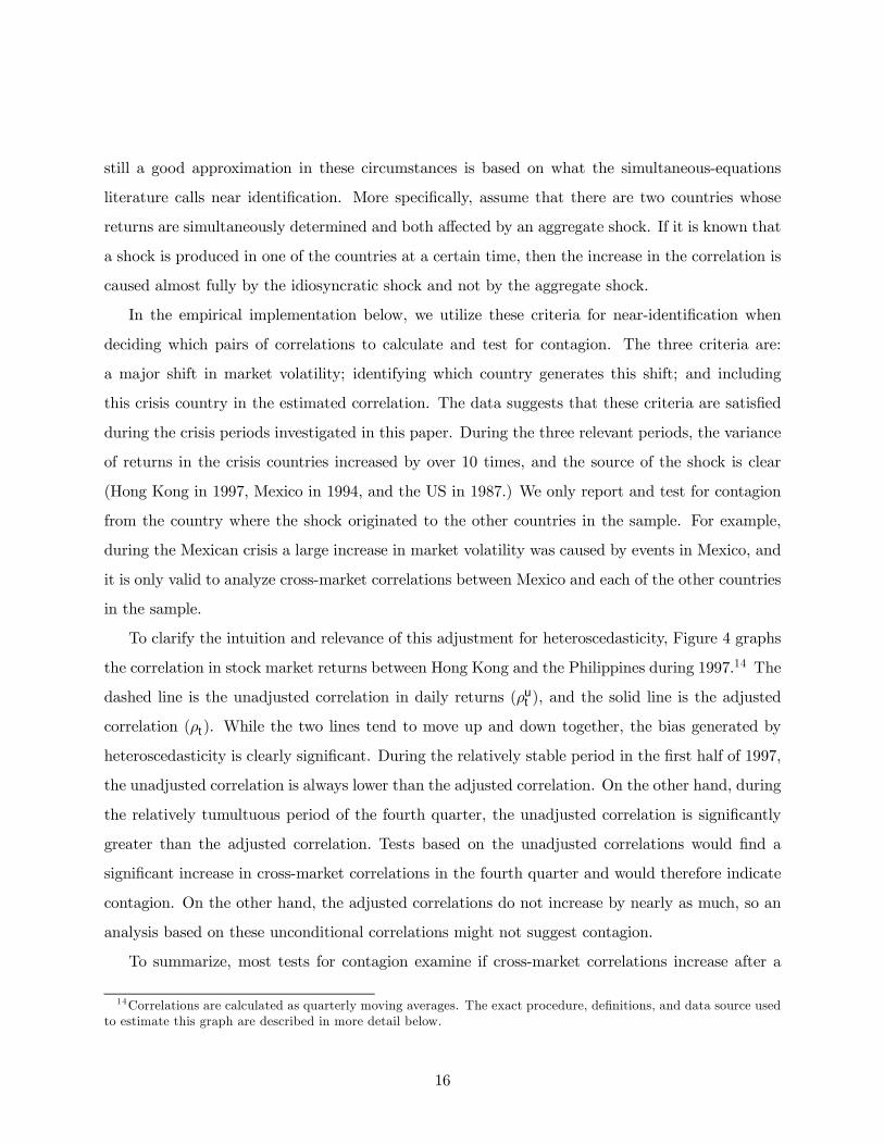
To clarify the intuition and relevance of this adjustment for heteroscedasticity, Figure 4 graphs

the correlation in stock market returns between Hong Kong and the Philippines during 1997.14 The

dashed line is the unadjusted correlation in daily returns (ρut ), and the solid line is the adjusted

correlation (ρt). While the two lines tend to move up and down together, the bias generated by

heteroscedasticity is clearly significant. During the relatively stable period in the first half of 1997,

the unadjusted correlation is always lower than the adjusted correlation. On the other hand, during

the relatively tumultuous period of the fourth quarter, the unadjusted correlation is significantly

greater than the adjusted correlation. Tests based on the unadjusted correlations would find a

significant increase in cross-market correlations in the fourth quarter and would therefore indicate

contagion. On the other hand, the adjusted correlations do not increase by nearly as much, so an

analysis based on these unconditional correlations might not suggest contagion.

To summarize, most tests for contagion examine if cross-market correlations increase after a

14Correlations are calculated as quarterly moving averages. The exact procedure, definitions, and data source usedto estimate this graph are described in more detail below.

16

0.0

0.1

0.2

0.3

0.4

0.5

0.6 01

/01/

9702

/01/

9703

/01/

9704

/01/

9705

/01/

9706

/01/

9707

/01/

9708

/01/

9709

/01/

9710

/01/

9711

/01/

9712

/01/

9701

/01/

98

Una

djus

ted

Adju

sted

Figure 4: Cross-Market Correlations: Hong Kong and the Philippines.

17

shock. Since the correlation coefficient central to this analysis is biased upward during periods

of market turmoil, estimated correlation coefficients will increase—even though actual correlations

may remain relatively constant. This could incorrectly lead to the conclusion that contagion occurs.

The remainder of this paper examines if this bias from heteroscedasticity has a significant impact

on estimates of cross-market correlations and tests for contagion during the 1997 East Asian crisis,

the 1994 Mexican peso collapse, and the 1987 US stock market crash.

3.2 The Data and Sample

Before performing these tests for contagion, it is necessary to briefly discuss our data and sample. To

calculate stock market returns, we utilize daily values of aggregate stock market indices reported

by Datastream. We perform each analysis using market returns measured in US dollars and in

local currency, and in most cases, the currency unit does not affect our central findings. Since

US dollar returns are used more frequently in previous work on contagion, and also to avoid an

unnecessary repetition of results, we focus on estimates based on US dollars in the discussion

below. (We continue to report estimates based on local returns if results are significantly different.)

Moreover, US dollar returns have the additional advantage of controlling for inflation (under non-

fixed exchange rate regimes).

Next, given this data set, it is necessary to choose which markets on which to focus. Most of the

work discussed in Section 2 examines a small sample of countries-often just the three largest markets

or stock markets in industrial countries. This was a logical choice for the time period many of these

papers covered (around 1987), because stock markets in most emerging economies were small and

restricted-if they even existed at all. With such a limited sample, however, it is obviously difficult

to draw any conclusions about contagion within emerging markets or between developed economies

and emerging markets. Since we would like to investigate each of these forms of contagion, and

especially since the liquidity of many emerging markets has increased over the past few years, this

paper substantially augments earlier samples. It considers the relative movements of twenty-eight

markets: the twenty-four largest markets (as ranked by market capitalization at the end of 1996),

plus the Philippines (to expand coverage of East Asia), Argentina and Chile (to expand coverage of

Latin America), and Russia (to expand coverage of emerging markets outside of these two regions.)

18

Table 1 lists these countries with total stock market capitalizations and average market volumes.15

It also defines the regions utilized throughout this paper.

Region Country Market Cap.(Bn US$)

Value Traded(Bn US$)

East Hong Kong 449.4 166.4Asia Indonesia 91.0 32.1

Japan 3088.9 1251.9Korea 138.9 177.3Malaysia 307.2 173.6Philippines 80.6 25.5Singapore 150.2 42.7Taiwan 273.6 470.2Thailand 99.8 44.4

Latin Argentina 44.7 -America Brazil 262.0 112.1

Chile 65.9 8.5Mexico 106.5 43.0

OECD Australia 311.9 145.5Belgium 119.8 26.1Canada 486.3 265.4France 591.1 277.1Germany 670.9 768.7Italy 258.2 102.4Netherlands 378.7 339.5Spain 242.8 249.1Sweden 247.2 136.9Switzerland 402.1 392.8UK 1740.3 578.5US 8484.4 7121.5

Other India 122.6 109.5Emerging Russia 37.2 -Markets South Africa 241.6 27.2

Table 1: Stock Market Characteristics

4 Contagion During the 1997 East Asian Crisis

As our first analysis of the impact of bias in the correlation coefficient, we test for contagion during

the East Asian crisis of 1997. As shown in Figure 1, stock market values in East Asia fluctuated

wildly in the later half of 1997, and many of these movements were mirrored, to varying degrees, in

stock markets around the world. One difficulty in testing for contagion during this period is that

there is no single event which acts as a clear catalyst behind this turmoil. For example, during June

the Thai market plummeted, during August the Indonesian market cratered, and in mid-October

15Source: International Finance Corporation. Emerging Stock Market Factbook. 1997.

19

the Hong Kong market crashed. A review of American and British newspapers and periodicals

during this period, however, shows an interesting pattern. The press paid little attention to the

earlier movements in the Thai and Indonesian markets (and, in fact, paid little attention to any

movements in East Asia) until the mid-October crash in Hong Kong. After the Hong Kong crash,

events in Asia became headline news, and an avid discussion quickly began on the East Asian

“crisis” and the possibility of “contagion” to the rest of the world. Therefore, for our base analysis

in this section, we focus on tests for contagion from Hong Kong to the rest of the world during

the tumultuous period directly after the Hong Kong crash. It is obviously possible that contagion

occurred during other periods of time, or from the combined impact of turmoil in a group of

East Asian markets instead of a single country. We test for these various types of contagion in the

sensitivity analysis below and show that using these different sources of contagion has no significant

impact on key results.

Using the October crash of the Hong Kong market as the most likely event to drive contagion,

we define our period of turmoil as the one month starting on October 17, 1997 (the start of this

visible Hong Kong crash). We define the period of relative stability as lasting from January 1,

1996 to the start of the period of turmoil.16 While this choice of dates may appear capricious,

the extensive robustness tests performed below will show that period definition does not affect the

central results. Next, the specification which we estimate is:

Xt = φ(L)Xt +Φ(L)It + ηt (7)

Xt ≡nxHK

t , xjt

o0

It ≡niHKt , iUS

t , ijt

o0(8)

where xHKt is the rolling-average, two-day return in the Hong Kong market, xj

t is the rolling-average,

two-day return in market j, Xt is the correlation between these two markets, φ(L) and Φ(L) are

vectors of lags, iHKt , iUS

t , ijt are short-term interest rates for Hong Kong, the US and country j,

respectively, and ηt is a vector of reduced-form disturbances. We utilize average two-day returns

16We do not utilize a longer length of time for the stability period due to the fact that any structural change inmarkets over this period would invalidate our test for contagion.

20

to control for the fact that markets in different countries are not open during the same hours. For

example, Latin American markets were closed at the time of the Hong Kong crash, so any impact

on Latin America would be reflected in market returns for the following day. The robustness tests

reported below show that the use of daily or weekly returns will not affect the central results. We

utilize five lags for φ(L) and Φ(L) in order to control for any within-week variation in trading

patterns. As also shown below, the number of lags does not significantly affect results. We include

interest rates in this equation in order to control for any aggregate shocks and/or monetary policy

coordination (as discussed in Section 2.) Although interest rates are an imperfect measure of

aggregate shocks, they are a good proxy for global shifts in real economic variables and/or policies

which affect stock market performance. We also show that excluding interest rates, or including

different combinations of interest rates, will not impact our central results.

Using this specification, we perform the standard test for stock market contagion described in

Section 2. We estimate the variance-covariance matrices during the period of turmoil and the full

period (including both the periods of relative stability and turmoil), and then use these matrices

to calculate correlations between Hong Kong and each of the other markets in our sample. We use

the asymptotic distribution of the standard, unadjusted correlation coefficient and do not adjust

this coefficient to account for the bias introduced by heteroscedasticity. Finally, we use a t-test

to evaluate if there is a significant increase in these correlation coefficients during the period of

turmoil.17 If ρ is the correlation during the full period and ρht is the correlation during the turmoil

period, the test hypotheses are:

H0 : ρ ≥ ρht

H1 : ρ < ρht

The estimated, unadjusted correlation coefficients for the period of stability, period of turmoil,

and full period are shown in Table 2. The critical value for the t-test at the 5% level is 1.65, so any

test statistic greater than this critical value indicates contagion (C), while any statistic less than

this value indicates no contagion (N). Test statistics and results are also reported in the table.

17We have also experimented with a number of other tests, and in each case, the test specification has no significantimpact on results.

21

Stability Turmoil Full Period TestRegion Country ρ σ ρ σ ρ σ Stat. Contag?East Indonesia 0.381 0.040 0.749 0.146 0.428 0.037 1.75 CAsia Japan 0.231 0.044 0.559 0.229 0.263 0.042 1.09 N

Korea 0.092 0.046 0.683 0.178 0.173 0.044 2.30 CMalaysia 0.280 0.043 0.465 0.261 0.288 0.041 0.58 NPhilippines 0.294 0.042 0.705 0.168 0.323 0.041 1.83 CSingapore 0.341 0.041 0.493 0.252 0.348 0.040 0.50 NTaiwan 0.010 0.046 0.149 0.326 0.028 0.046 0.33 NThailand 0.046 0.046 0.402 0.279 0.082 0.045 0.99 N

Latin Argentina 0.030 0.046 -0.144 0.326 0.004 0.046 -0.40 NAmerica Brazil 0.105 0.046 -0.593 0.332 0.080 0.045 -0.37 N

Chile 0.144 0.045 0.619 0.206 0.197 0.044 1.69 CMexico 0.238 0.044 0.241 0.314 0.238 0.043 0.01 N

OECD Australia 0.356 0.040 0.865 0.084 0.431 0.037 3.59 CBelgium 0.140 0.045 0.714 0.163 0.178 0.044 2.58 CCanada 0.145 0.045 0.378 0.286 0.170 0.044 0.63 NFrance 0.227 0.044 0.886 0.072 0.299 0.042 5.19 CGermany 0.383 0.039 0.902 0.062 0.450 0.036 4.60 CItaly 0.175 0.045 0.896 0.066 0.236 0.043 6.05 CNetherlands 0.319 0.042 0.742 0.150 0.347 0.040 2.08 CSpain 0.191 0.045 0.878 0.076 0.269 0.042 5.14 CSweden 0.233 0.044 0.796 0.122 0.298 0.042 3.04 CSwitzerland 0.183 0.045 0.842 0.097 0.232 0.043 4.34 CUK 0.255 0.043 0.615 0.201 0.280 0.042 1.34 NUS 0.021 0.046 -0.390 0.285 -0.027 0.046 -1.11 N

Other India 0.097 0.046 0.024 0.333 0.089 0.045 -0.17 NEmerging Russia 0.026 0.043 0.866 0.084 0.365 0.040 4.07 CMarkets S. Africa 0.368 0.040 0.852 0.092 0.455 0.036 3.10 C

Table 2: 1997 East Asian Crises: Unadjusted Correlation Coefficients

22

Several patterns are immediately apparent. First, cross-market correlations during the rela-

tively stable period are not surprising. Hong Kong is highly correlated with Australia and many

of the East Asian economies, and much less correlated with the Latin American markets. Second,

cross-market correlations between Hong Kong and most of the other countries in the sample in-

crease during the turmoil period. This is a prerequisite for contagion to occur. This change is

especially notable in many of the OECD markets, where the average correlation with Hong Kong

increases from 0.22 during the stability period to 0.68 during the turmoil period. In one extreme

example, the correlation between Hong Kong and Belgium increases from 0.14 in the period of

stability to 0.71 in the period of turmoil. Third, the t-tests indicate a significant increase in this

unadjusted correlation coefficient during the turmoil period for fifteen countries. According to the

interpretation standard in this literature, this implies contagion occurred from the October crash

of the Hong Kong market to Australia, Belgium, Chile, France, Germany, Indonesia, Italy, Korea,

the Netherlands, the Philippines, Russia, South Africa, Spain, Sweden, and Switzerland. As dis-

cussed above, however, these increases in the correlation coefficient might result from a bias due to

heteroscedasticity and not actually constitute contagion.

To test how this bias in the correlation coefficient affects our tests for contagion, we repeat this

analysis but use the correction in equation 6 to adjust for this bias. In other words, we repeat

the above analysis using the unconditional instead of the conditional correlation coefficients.18

Estimated, adjusted correlation coefficients and test results are shown in Table 3.

It is immediately apparent that adjusting for the bias from heteroscedasticity has a significant

impact on estimated cross-market correlations and the resulting tests for contagion. In each country,

the adjusted correlation is substantially smaller (in absolute value) than the unadjusted correlation

during the turmoil period and is slightly greater in the stability period. For example, during the

turmoil period, the average unadjusted correlation for the entire sample is 0.53 while the average

adjusted correlation is 0.32. During the stability period, the average unadjusted correlation is 0.20

while the average adjusted correlation is 0.22. In many cases, the adjusted correlation coefficient

is still greater during the turmoil period than the full period, but this increase is significantly

diminished from that found in Table 2. For example, the unadjusted correlation between Hong

Kong and the Netherlands jumps from 0.35 during the full period to 0.74 during the turmoil

18We continue to use the asymptotic distribution of this adjusted correlation coefficient.

23

Stability Turmoil Full Period TestRegion Country ρ σ ρ σ ρ σ Stat. Contag?East Indonesia 0.413 0.042 0.399 0.244 0.428 0.037 -0.10 NAsia Japan 0.252 0.045 0.255 0.290 0.263 0.042 -0.02 N

Korea 0.098 0.046 0.380 0.257 0.173 0.044 0.69 NMalaysia 0.305 0.044 0.200 0.304 0.288 0.042 -0.26 NPhilippines 0.315 0.044 0.388 0.253 0.323 0.041 0.22 NSingapore 0.348 0.043 0.343 0.288 0.348 0.040 -0.02 NTaiwan 0.010 0.046 0.058 0.331 0.028 0.046 0.08 NThailand 0.051 0.046 0.171 0.312 0.082 0.045 0.25 N

Latin Argentina 0.033 0.046 -0.059 0.331 0.004 0.046 -0.17 NAmerica Brazil 0.113 0.046 -0.025 0.333 0.080 0.045 -0.28 N

Chile 0.157 0.046 0.302 0.277 0.197 0.044 0.33 NMexico 0.256 0.045 0.102 0.326 0.238 0.043 -0.37 N

OECD Australia 0.385 0.042 0.561 0.191 0.431 0.037 0.57 NBelgium 0.153 0.046 0.371 0.254 0.178 0.044 0.65 NCanada 0.159 0.046 0.156 0.315 0.170 0.044 -0.04 NFrance 0.248 0.045 0.596 0.177 0.299 0.042 1.35 NGermany 0.412 0.042 0.642 0.162 0.450 0.036 0.97 NItaly 0.191 0.045 0.618 0.170 0.236 0.043 1.79 CNetherlands 0.346 0.043 0.397 0.246 0.347 0.040 0.18 NSpain 0.209 0.045 0.584 0.182 0.269 0.042 1.40 NSweden 0.255 0.045 0.454 0.226 0.298 0.042 0.58 NSwitzerland 0.200 0.045 0.519 0.205 0.232 0.043 1.16 NUK 0.278 0.044 0.292 0.279 0.280 0.042 0.04 NUS 0.023 0.046 -0.169 0.313 -0.027 0.046 -0.40 N

Other India 0.101 0.046 0.009 0.333 0.089 0.045 -0.21 NEmerging Russia 0.285 0.044 0.569 0.188 0.365 0.040 0.89 NMarkets S. Africa 0.389 0.042 0.592 0.186 0.455 0.036 0.62 N

Table 3: 1997 East Asian Crises: Adjusted Correlation Coefficients

24

period, while the adjusted correlation only increases from 0.35 to 0.40. Moreover, when tests for

contagion are performed on these adjusted correlations, only one coefficient (for Italy) increases

significantly during the turmoil period. In other words, there is only evidence of contagion from

the Hong Kong crash to one other country in the sample (versus fifteen cases of contagion when

tests are based on the unadjusted coefficients.)

These results highlight exactly what we mean by contagion. Many stock markets are highly cor-

related with Hong Kong’s market during this tumultuous period in October and November of 1997.

For example, during this period the unconditional correlation between Hong Kong and Australia is

0.56 and that between Hong Kong and the Philippines is 0.39. These high cross-market correlations

do not signify contagion, however, because these markets are also highly correlated during periods

of relative stability. These stock markets are highly interdependent, both in periods of stability

and turmoil, and are closely linked through trade and/or other real economic fundamentals. A

continued high level of interdependence after a crisis does not constitute contagion.

4.1 Robustness Tests

Since this “no contagion, only interdependence” result is so controversial, and especially since

the adjustment to the correlation coefficient has such a significant impact on our analysis, we

perform an extensive array of robustness tests. In the following sections we test for the impact

of: adjusting the frequency of returns and lag structure, modifying period definitions, altering the

source of contagion, varying the interest rate controls, and estimating local currency returns. In

each case (as well as others not reported below), the central result does not change. Tests based

on the unadjusted correlation coefficients find some evidence of contagion, while tests based on

the adjusted coefficients find virtually no evidence of contagion. Due to the repetition of these

robustness tests, we only report summary results for each analysis.19 We do, however, discuss any

findings which are significantly different than those reported above.

4.1.1 Adjusting the Frequency of Returns and Lag Structure

As a first set of robustness tests, we adjust the frequency of returns and/or lag structure from that

used above. In our base analysis, we focus on rolling-average, two-day returns in order to control

19Complete results are available from the authors.

25

for the fact that different stock markets are not open during the same hours. We also include five

lags of the cross-market correlations (Xt) and the vector of interest rates (It) in order to control

for any within-week variation in trading patterns. We repeat this analysis using daily returns and

weekly returns. We also combine each of these return calculations with zero, one, or five lags (as

possible) of Xt and It. Note that in each case, estimates are only consistent if there are at least

as many lags (minus one) as the number of days averaged to calculate the returns.20 Results are

reported in Table 4.

Return Frequency Cases of Contagionand Lag Structure Unadjusted ρ Adjusted ρ

daily + 0 lags 17 0daily + 1 lag 17 0daily + 5 lags 17 1

2 day + 1 lag 15 02 day + 5 lags 15 1weekly + 5 lags 13 2

Table 4: 1997 East Asian Crises: Robustness to Adjusting the Frequency of Returns and/or LagStructure

This table shows that adjusting the frequency of returns and/or lag structure does not sig-

nificantly change our central results. When cross-market correlations are estimated based on the

unadjusted correlation coefficient, there is evidence of contagion from Hong Kong to about half the

sample. When cross-market correlations are based on the adjusted correlations, there is almost no

evidence of contagion. No matter which frequency of returns and number of lags are included in

the estimation of equation 7, there are at most two cases where cross-market correlations increase

significantly after the October crash of the Hong Kong market.

20Lags are required because we utilize a moving average to measure returns. Therefore, by construction, obser-vations at time t are correlated with those at t − 1, t − 2, etc. There are two methods of solving this problem.First, include lags in the regression (as we do). Second, change the frequency of the data and reduce the number ofobservations. If there are no holidays, or the holidays are the same across countries then both procedures should beidentical. If the missing observations differ across countries (as they do in our sample), it is easier to control for thisproblem using the first technique.Also note that we do not use more than five lags due to the short length of the turmoil period.

26

4.1.2 Modifying Period Definitions

For a second set of robustness tests, we modify definitions for the periods of turmoil and relative

stability. In our base estimation, we define the period of turmoil as starting on October 17, 1997 (the

start of the publicized Hong Kong crash ) and lasting one month. We repeat this analysis, extending

this turmoil period to either: start on June 1, 1997 (when the Thai market first crashed); start on

August 7,1997 (when the Indonesian and Thai markets began their simultaneous, dramatic one-

month plunge); or end on March 1, 1998 (the end of the sample). Also, in the original estimation,

we define the period of relative stability as lasting from January 1, 1996 through October 16, 1997.

We extend this period by three years and one year. Summary results based on these different period

definitions are reported in Table 5.

Turmoil Stability Cases of ContagionPeriod Period Unadjusted ρ Adjusted ρ

10/17/97 - 11/16/97 01/01/96 - 10/16/97 15 1

06/01/97 - 11/16/97 01/01/96 - 05/31/97 2 008/07/97 - 11/16/97 01/01/96 - 08/06/97 7 010/17/97 - 03/01/98 01/01/96 - 10/16/97 16 0

10/17/97 - 11/16/97 01/01/93 - 10/16/97 17 010/17/97 - 11/16/97 01/01/95 - 10/16/97 16 1

Table 5: 1997 East Asian Crises: Robustness to Modifying Period Definitions

Modifying the definitions of the turmoil or stability periods does not change the central result;

there is virtually no evidence of contagion when tests are based on the adjusted correlation coeffi-

cients. Moreover, it is interesting to note that when the turmoil period is extended to before the

dramatic Hong Kong crash, tests based on the unadjusted correlation coefficients indicate much

less contagion. When the turmoil period is extended after the Hong Kong crash, however, tests

based on the unadjusted correlation coefficients do indicate contagion. This is not surprising, given

that market volatility increased significantly after the Hong Kong crash (and it is this volatility

that generates a bias in the unadjusted correlation coefficient.) This also supports our hypothesis

that the Hong Kong crash is the most likely catalyst driving any contagion.

27

4.1.3 Altering the Source of Contagion

As a third sensitivity test, we examine how altering the defined source of contagion can impact our

results. As discussed above, one difficulty in testing for contagion during the East Asian crisis is

that there is no single event acting as a clear catalyst driving this turmoil. For example, during

June the Thai market plummeted, during August the Indonesian market cratered, and in October

the Hong Kong market crashed. We focus on the Hong Kong crash as the impetus behind any

contagion due to the sudden change in global sentiment after this event. It was not until the Hong

Kong crash that concerns about Asia became headline news, and the discussion began on the East

Asian “crisis” and the possibility of “contagion” to the rest of the world. In this section, we test

if events in other countries, or even groups of countries, would be a more accurate catalyst driving

contagion during the later half of 1997.

We begin by testing for contagion from single East Asian markets after a significant downturn

in those markets. For example, we test for contagion from Thailand after its June crash, from

Thailand or Indonesia after their August crashes, or from Korea after its two-month crash starting

in late October. (In each case, we end the stability period directly before the crash.)

Next, since contagion may occur from the combined impact of movements in several East

Asian markets, instead of movement in any one market, we construct several indices of East Asian

markets. For each index, we weight each country by total market capitalization at the end of 1996,

as reported in Table 1. We test for contagion: from Thailand and Indonesia after the August

crashes in both of these markets; from Hong Kong and Korea during several tumultuous periods

in these markets; and from Hong Kong, Indonesia, Korea, Malaysia, and Thailand (a five-country

index) during several different periods. Summary results for all of these tests are reported in Table

6.

This table shows that altering the source of contagion during the East Asian crisis does not

significantly change our central results.21 Tests for contagion based on single East Asian markets

21Also note that for each of these alternative sources of contagion, we have performed the same senstivity tests asreported for the Hong Kong base case (i.e. adjusting the frequency of returns and lag structure, modifying perioddefinitions, changing the controls for aggregate shocks, and estimating local currency returns.)

28

Contagion Cases of ContagionSource Turmoil Period Full Period Unadjusted ρ Adjusted ρ

Hong Kong 10/17/97 - 11/16/97 01/01/96 - 11/16/97 15 1

Thailand 06/01/97 - 06/30/97 01/01/96 - 06/30/97 0 0Thailand 08/07/97 - 09/06/97 01/01/96 - 09/06/97 2 0Indonesia 08/07/97 - 09/06/97 01/01/96 - 09/06/97 5 0Korea 10/23/97-12/22/97 01/01/96 - 12/22/97 0 0

Indon., Thail. 08/07/97 - 09/06/97 01/01/96 - 09/06/97 7 0H.K., Korea 10/17/97 - 11/16/97 10/17/97 - 11/16/97 16 2H.K., Korea 10/17/97 - 12/23/97 01/01/96 - 12/23/97 12 0H.K., Korea 10/17/97 - 03/01/97 01/01/96 - 03/01/98 0 0

5-country index 10/17/97 - 12/23/97 01/01/96 - 12/23/97 6 05-country index 08/07/97 - 12/23/97 01/01/96 - 12/23/97 2 05-country index 08/07/97 - 03/01/98 01/01/96 - 03/01/98 7 0

Table 6: 1997 East Asian Crises: Robustness to Altering the Source of Contagion

or indices combining these markets all indicate that there was virtually no contagion from these

sources to markets around the world.

4.1.4 Varying the Interest Rate Controls

For a fourth robustness test, we vary the interest rate controls. As discussed in Section 2, we utilize

interest rates to control for any aggregate shocks and/or monetary policy coordination which could

simultaneously affect different stock markets. Specifically, in the formulation of equation 7 we

control for interest rates in Hong Kong, the US and country j. We repeat this analysis using

no controls for interest rates, just controlling for the US interest rate (as a measure of aggregate

shocks) and just controlling for interest rates in Hong Kong and country j (to control for monetary

policy coordination.) Table 7 summarizes these results.

This table clearly shows that our results are highly robust to changing the interest rates controls,

or even eliminating them completely.

4.1.5 Utilizing Local Currency Returns

As a final sensitivity test, we repeat the previous tests utilizing returns based on local currency

instead of US dollars. Test results based on local currency returns, with a number of different lag

29

Interest Rates Cases of ContagionIncluded Unadjusted ρ Adjusted ρ

iHKt , iUS

t , ijt 15 1

None 15 0iUSt 15 0

iHKt , ijt 15 0

Table 7: 1997 East Asian Crises: Robustness to Varying the Interest Rate Controls

and return structures, are reported in Table 8.

Return Frequency Cases of Contagionand Lag Structure Unadjusted ρ Adjusted ρ

daily + 0 lags 14 0daily + 1 lag 14 0daily + 5 lags 16 1

2 day + 1 lag 16 12 day + 5 lags 14 2weekly + 5 lags 12 4

Table 8: 1997 East Asian Crises: Robustness Tests Based on Local Currency Returns

Measuring returns based on local currencies instead of US dollars clearly has minimal impact

on our central results.

4.1.6 Summary: Robustness Tests

In our base test for contagion during the 1997 East Asian crisis, we find evidence of contagion

between Hong Kong and 15 countries when tests are based on the unadjusted correlation coefficients.

When the same tests are based on the adjusted correlation coefficients, there is only one case of

contagion. We perform an extensive array of tests to see if these results are robust. We adjust the

frequency of returns and/or lag structure, modify period definitions, alter the source of contagion,

vary the interest rate controls, and estimate local currency returns. In each case, the central

result does not change. When tests are based on the unadjusted correlation coefficients, there is

evidence of contagion in about half the sample (with the number of cases highly dependent on the

specification estimated), but when tests are based on the adjusted coefficients, there is virtually no

evidence of contagion.

30

Therefore, these results suggest far less contagion from the East Asian crisis than previously

believed. Unconditional, cross-market correlations between Hong Kong and each of the countries

in our sample (with the possible exception of Italy) did not increase significantly after the Hong

Kong crash in October of 1997. High correlations between Hong Kong and any other markets

during this period did not result from a significant shift in cross-market linkages. Instead, any

high cross-market correlations during this tumultuous period reflect continued interdependence,

not contagion, across countries.

5 Contagion During the 1994 Mexican Peso Crisis

As our second set of analyses of how the bias in the correlation coefficient affects tests for contagion,

we compare cross-market correlations before and after the Mexican peso crisis of 1994. In December

of 1994, the Mexican government suffered a balance of payments crisis, leading to a collapse of the

peso and a crash in the Mexican stock market. This crisis generated fears that contagion could

quickly lead to crises in other emerging markets and especially in the rest of Latin America. This

analysis is more straightforward than that during the East Asian crisis due to the existence of one

clear catalyst (the collapse of the peso) driving any contagion.

For our base test, we define the period of turmoil in the Mexican market as lasting from

12/19/94 (the day the exchange rate regime was abandoned) through 12/31/94. We define the

period of relative stability as 1/1/93 through 12/31/95 (excluding the period of turmoil). Next,

we estimate the same system of equations as above (equation 7), but replace returns and interest

rates for Hong Kong with those of Mexico. We continue to calculate returns as rolling, two-day

averages and to utilize five lags for φ(L) and Φ(L). Then we repeat the standard test for stock

market contagion: test for a significant increase in cross-market correlations during the period of

turmoil in the Mexican market. Estimates of the unadjusted correlation coefficients and test results

are shown in Table 9.

These unadjusted correlation coefficients show many patterns similar to the East Asian case.

First, during the relatively stable period, the Mexican market tends to be more highly correlated

with markets in the same region (such as other Latin American countries and the US). Second,

cross-market correlations between Mexico and most countries in the sample increase during the

31

Stability Turmoil Full Period TestRegion Country ρ σ ρ σ ρ σ Stat. Contag?East Hong Kong 0.055 0.037 0.467 0.391 0.070 0.036 0.93 NAsia Indonesia 0.042 0.037 0.194 0.481 0.049 0.036 0.28 N

Japan 0.028 0.037 0.426 0.409 0.036 0.036 0.87 NKorea 0.035 0.037 0.721 0.240 0.058 0.036 2.40 CMalaysia 0.048 0.037 -0.064 0.498 0.042 0.036 -0.20 NPhilippines 0.066 0.037 -0.067 0.498 0.061 0.036 -0.24 NSingapore 0.068 0.037 0.194 0.481 0.070 0.036 0.24 NTaiwan 0.092 0.036 0.526 0.362 0.097 0.036 1.08 NThailand 0.047 0.037 0.101 0.495 0.045 0.036 0.10 N

Latin Argentina 0.382 0.031 0.859 0.131 0.401 0.031 2.84 CAmerica Brazil 0.384 0.031 0.791 0.187 0.402 0.031 1.79 C

Chile 0.309 0.033 0.426 0.409 0.298 0.033 0.29 N

OECD Australia 0.078 0.036 0.565 0.340 0.092 0.036 1.26 NBelgium 0.039 0.037 0.636 0.298 0.052 0.036 1.75 CCanada 0.136 0.036 0.333 0.444 0.135 0.036 0.41 NFrance 0.097 0.036 0.139 0.490 0.093 0.036 0.09 NGermany 0.001 0.037 0.332 0.444 0.011 0.036 0.67 NItaly -0.002 0.037 -0.504 0.373 -0.016 0.036 -1.19 NNetherlands 0.044 0.037 0.652 0.288 0.054 0.036 1.84 CSpain 0.139 0.036 0.120 0.492 0.134 0.036 -0.03 NSweden 0.105 0.036 -0.213 0.477 0.095 0.036 -0.60 NSwitzerland 0.005 0.037 0.182 0.483 0.010 0.036 0.33 NUK 0.097 0.036 0.284 0.460 0.096 0.036 0.38 NUS 0.207 0.035 0.118 0.493 0.196 0.035 -0.15 N

Other India 0.013 0.037 -0.017 0.500 0.012 0.036 -0.05 NEmerging Russia -0.009 0.037 0.077 0.497 -0.008 0.036 0.16 NMarkets S. Africa 0.062 0.037 0.710 0.248 0.073 0.036 2.24 C

Table 9: 1994 Mexican Peso Crisis: Unadjusted Correlations in Stock Market Returns

32

period of turmoil. This is a prerequisite for contagion to occur. Many developed countries which

are not highly correlated with Mexico during the period of stability become highly correlated

during the period of turmoil. Third, the t-tests indicate that there is a significant increase (at the

5% level) in the correlation coefficient during the turmoil period for six countries. According to

the interpretation used in previous empirical work, this indicates that contagion occurred from the

crash of the Mexican stock market in 1994 to Argentina, Belgium, Brazil, Korea the Netherlands,

and South Africa. As discovered above, however, these increases in the correlation coefficient might

not actually constitute contagion. Instead, they may result from the bias due to increased market

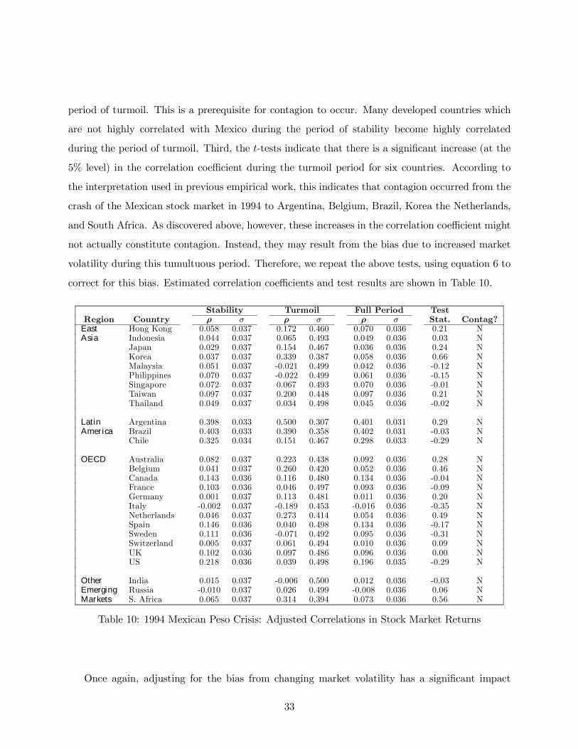
volatility during this tumultuous period. Therefore, we repeat the above tests, using equation 6 to

correct for this bias. Estimated correlation coefficients and test results are shown in Table 10.

Stability Turmoil Full Period TestRegion Country ρ σ ρ σ ρ σ Stat. Contag?

East Hong Kong 0.058 0.037 0.172 0.460 0.070 0.036 0.21 NAsia Indonesia 0.044 0.037 0.065 0.493 0.049 0.036 0.03 N

Japan 0.029 0.037 0.154 0.467 0.036 0.036 0.24 NKorea 0.037 0.037 0.339 0.387 0.058 0.036 0.66 NMalaysia 0.051 0.037 -0.021 0.499 0.042 0.036 -0.12 NPhilippines 0.070 0.037 -0.022 0.499 0.061 0.036 -0.15 NSingapore 0.072 0.037 0.067 0.493 0.070 0.036 -0.01 NTaiwan 0.097 0.037 0.200 0.448 0.097 0.036 0.21 NThailand 0.049 0.037 0.034 0.498 0.045 0.036 -0.02 N

Latin Argentina 0.398 0.033 0.500 0.307 0.401 0.031 0.29 NAmerica Brazil 0.403 0.033 0.390 0.358 0.402 0.031 -0.03 N

Chile 0.325 0.034 0.151 0.467 0.298 0.033 -0.29 N

OECD Australia 0.082 0.037 0.223 0.438 0.092 0.036 0.28 NBelgium 0.041 0.037 0.260 0.420 0.052 0.036 0.46 NCanada 0.143 0.036 0.116 0.480 0.134 0.036 -0.04 NFrance 0.103 0.036 0.046 0.497 0.093 0.036 -0.09 NGermany 0.001 0.037 0.113 0.481 0.011 0.036 0.20 NItaly -0.002 0.037 -0.189 0.453 -0.016 0.036 -0.35 NNetherlands 0.046 0.037 0.273 0.414 0.054 0.036 0.49 NSpain 0.146 0.036 0.040 0.498 0.134 0.036 -0.17 NSweden 0.111 0.036 -0.071 0.492 0.095 0.036 -0.31 NSwitzerland 0.005 0.037 0.061 0.494 0.010 0.036 0.09 NUK 0.102 0.036 0.097 0.486 0.096 0.036 0.00 NUS 0.218 0.036 0.039 0.498 0.196 0.035 -0.29 N

Other India 0.015 0.037 -0.006 0.500 0.012 0.036 -0.03 NEmerging Russia -0.010 0.037 0.026 0.499 -0.008 0.036 0.06 NMarkets S. Africa 0.065 0.037 0.314 0.394 0.073 0.036 0.56 N

Table 10: 1994 Mexican Peso Crisis: Adjusted Correlations in Stock Market Returns

Once again, adjusting for the bias from changing market volatility has a significant impact

33

on estimated cross-market correlations and the resulting tests for contagion. In each country,

the adjusted correlation is substantially smaller (in absolute value) than the unadjusted correlation

during the turmoil period and is slightly greater in the stability period. In many cases, the adjusted

correlation coefficient is still greater during the turmoil period than during the stability period, but

this increase is significantly diminished from that found in Table 9. For example, for the full period,

the cross-market correlation between Mexico and Argentina is 0.40. In the period of turmoil, the

unadjusted correlation jumps to 0.86, while the adjusted correlation jumps to only 0.50. When

tests for contagion are performed on these adjusted correlations, there is not one case in which

the correlation coefficient increases significantly during the turmoil period. In other words, there

is no longer evidence of contagion from Mexico in 1994 to any other country in the sample. Even

Argentina and Brazil, which were frequently cited as examples of contagion after the Mexican peso

crisis, are not subject to contagion (as defined in this paper).

An extensive set of robustness tests supports these central results. We adjust the frequency of

returns and lag structure, modify period definitions, vary the interest rate controls, and/or estimate

local currency returns. While the evidence of contagion based on the unadjusted coefficient does

vary (from 0 to 7) based on the specification estimated, whenever the coefficient is adjusted to

remove any bias from heteroscedasticity, there is virtually no evidence of contagion.22

Therefore, these results suggest that there was minimal (if any) contagion from the Mexican

peso crisis. Cross-market correlations between Mexico and each of the countries in our sample

never increase significantly after the collapse of the peso (when returns are measured in US dol-

lars). Any markets which are highly correlated with Mexico during this period of turmoil are also

highly correlated during periods of relative stability. For example, the Mexican and Argentinian

markets are highly correlated after the Mexican peso collapse—with an unconditional correlation

coefficient of 0.50. This is not contagion, however, because these two markets are traditionally

highly correlated—with an unconditional correlation coefficient during the entire period of 0.40.

Cross-market correlations are therefore not significantly different during the peso crisis. These two

stock markets are highly interdependent, both in periods of stability and turmoil. They are closely

linked through trade and other real economic fundamentals.

22 In all of these tests based on the adjusted coefficients, there are never more than two cases of contagion. Thesecases only occur when returns are measured in local currency, and often occur in unexpected countries, such as Indiaand South Africa.

34

6 Contagion During the 1987 US Stock Market Crash

Before the East Asian crisis and Mexican peso collapse, another period of stock market turmoil

when investors feared contagion was after the US stock market crash in October of 1987. As

discussed in the literature review of Section 2, this period is the focus of most empirical work on

stock market contagion. To test for contagion during this period, we repeat the test procedure

described above. We define the period of turmoil as October 17, 1987 (the date of the original

crash) through December 4, 1987 (the nadir of the US market) and define the period of relative

stability as January 1, 1986 through the October crash. Since many of the smaller stock markets

in our sample of 28 countries were not in existence or were highly regulated at this time, we focus

only on the ten largest stock markets (including the US). Once again, we focus on two-day, rolling-

average, US dollar returns and control for five lags of returns and interest rates. Results based on

the unadjusted and adjusted correlation coefficients are reported in Tables 11 and 12.

Stability Turmoil Full Period TestCountry ρ σ ρ σ ρ σ Stat. Contag?Australia -0.199 0.045 -0.106 0.202 -0.180 0.044 0.30 NCanada 0.515 0.034 0.635 0.122 0.531 0.032 0.68 NFrance 0.169 0.045 0.610 0.128 0.256 0.042 2.08 CGermany 0.105 0.046 0.492 0.155 0.172 0.044 1.61 NHong Kong 0.154 0.045 0.091 0.202 0.139 0.044 -0.20 NJapan -0.015 0.046 0.167 0.198 0.005 0.044 0.67 NNetherlands 0.246 0.044 0.662 0.115 0.325 0.040 2.18 CSwitzerland 0.160 0.045 0.552 0.142 0.221 0.043 1.79 CUK 0.145 0.045 0.645 0.119 0.212 0.043 2.67 C

Table 11: 1987 U.S. Stock Market Crash: Unadjusted Correlation Coefficients

Stability Turmoil Full Period TestCountry ρ σ ρ σ ρ σ Stat. Contag?Australia -0.209 0.045 -0.007 0.203 -0.180 0.044 0.46 NCanada 0.528 0.038 0.497 0.152 0.531 0.032 -0.18 NFrance 0.176 0.046 0.441 0.159 0.256 0.042 0.92 NGermany 0.110 0.046 0.352 0.176 0.172 0.044 0.82 NHong Kong 0.162 0.046 0.057 0.203 0.139 0.044 -0.33 NJapan -0.015 0.046 0.107 0.201 0.005 0.044 0.42 NNetherlands 0.256 0.045 0.500 0.149 0.325 0.040 0.93 NSwitzerland 0.165 0.046 0.431 0.165 0.221 0.043 1.01 NUK 0.150 0.046 0.502 0.150 0.212 0.043 1.50 N

Table 12: 1987 U.S. Stock Market Crash: Adjusted Correlation Coefficients

Most patterns are similar to those found after the 1997 East Asian crisis and 1994 Mexican peso

collapse. First, tests for a significant increase in cross-market correlations based on the unadjusted

correlation coefficients show a substantial amount of contagion—in almost one-half of the sample.

35

Second, when the correlation coefficients are adjusted to correct for changing market volatility,

these tests find no evidence of contagion. Third, many of the adjusted cross-market correlations

are relatively large during the period of turmoil, but since there is no significant change in cross-

market linkages, these large correlations indicate a high level of interdependence, and not contagion,

across countries.

Finally, as discussed in Section 4, these results may not be robust to: adjusting the frequency

of returns and lag structure; modifying period definitions; varying the interest rate controls; and

estimating local currency returns. We repeat each of these sensitivity tests and find that results are

extremely robust. When tests are based on the unadjusted correlation coefficient, there is always

contagion from the US to several markets after the October crash. When tests are based on the

adjusted correlation coefficients, there is never more than one case of contagion (and usually zero

cases). This is in sharp contrast to the papers discussed in Section 2. Each of these earlier papers

which tested for contagion after the 1987 US stock market crash found evidence of a significant

increase in cross-market linkages during this period. None of these papers, however, adjusted the

correlation coefficient to correct for heteroscedasticity. The extensive robustness tests performed

for this paper show that after adjusting the correlation coefficient to remove this bias, there is

virtually no evidence of contagion from the US to other major stock markets after the 1987 crash.

7 Conclusion and a New Puzzle

The first three sections of this paper discuss techniques for examining market co-movements and

testing for contagion. Contagion is narrowly defined as a significant increase in cross-market link-

ages after a shock to one country (or group of countries). Section 3 shows that the correlation

coefficient underlying conventional tests for contagion is biased. This correlation coefficient is ac-

tually conditional on market volatility over the time period under consideration, so that during

a period of turmoil when stock market volatility increases, unadjusted estimates of cross-market

correlations will be biased upward. This can erroneously lead us to accept that contagion occurred.

We show a simple method of adjusting the correlation coefficient to correct for this bias. This

adjusted correlation coefficient, while clearly an improvement over that used in past work measur-

ing stock market co-movements, can still be biased in the presence of endogeneity or unobservable

36

aggregate shocks.

The final three sections of the paper apply these concepts to test for contagion during three

periods of market turmoil: the 1997 East Asian crisis, the 1994 Mexican peso collapse, and the 1987

US stock market crash. Each section performs a number of tests evaluating if average cross-market

correlations increase significantly during the relevant period of turmoil. In each of these periods,

tests based on the unadjusted correlation coefficients suggest that there was contagion in several

markets. When the same tests are based on the adjusted correlation coefficients, however, the in-

cidence of contagion falls dramatically—to zero in most cases. Three key results continually emerge

from this battery of tests. First, when testing for contagion across stock markets, it is critically

important to measure market co-movements accurately. Adjusting the correlation coefficient to

correct for heteroscedasticity will not only affect estimates of cross-market correlations, but can

significantly reduce estimates of stock market contagion. Second, when these adjusted correlation

coefficients are applied to the standard tests for contagion, we find significantly less evidence of

contagion during the East Asian crisis, the Mexican peso collapse, and the US stock market crash,

than previously believed. In fact, in most of these tests, there is not a single case of contagion.

Third, when these results are combined with the observed high level of market co-movement during

these periods of market turmoil, it highlights exactly what we mean by contagion in this paper.

Contagion is not simply a high cross-market correlation after a shock. It is a significant increase

in this correlation after the shock. The high levels of co-movement across many stock markets

during these three tumultuous periods reflects a continuation of strong cross-market linkages, and

not a significant shift in these linkages. In other words, during the recent Asian crisis, the Mexi-

can peso collapse, and the 1987 US market crash, continued strong cross-market linkages suggest

interdependence instead of contagion.

These results are highly robust to: adjusting the frequency of returns and/or lag structure;

modifying period definitions; altering the source of contagion; varying the interest rate controls;

and estimating local currency returns. These results, however, should be interpreted cautiously

because the adjustment for heteroscedasticity may change in the presence of endogeneity and/or

aggregate shocks. The critical point of this paper and its extensive series of tests is that inferences

based on the unadjusted correlation coefficient can be extremely misleading. Simple adjustments

can reverse what appear to be straightforward conclusions. This paper presents a technique for

37

adjusting for one problem with the cross-market correlation coefficient: heteroscedasticity. Future

work needs to examine how endogeneity and aggregate shocks can affect this adjustment, as well

as designing new techniques to simultaneously correct for these three econometric problems.

Taken as a whole, these results suggest a new direction for research on stock market co-

movements. Stock markets in many countries are highly integrated, and this high level of co-

movement is fairly constant in all states of the world. There does not appear to be a significant

change in how markets are linked during crisis periods. This paper suggests that future research

does not need to focus on how international propagation mechanisms change after a shock. Instead,

research should focus on why markets are so highly integrated during periods of relative stability

(as well as periods of crisis). Crisis periods could be used as windows to help identify these trans-

mission mechanisms, instead of interpreted as periods which generate new types of transmission

mechanisms. In other words, we should focus not on why some countries are so vulnerable during

periods of crisis, but why countries are always so vulnerable to movements in other countries. Why

do so many markets of such different sizes, structures, and geographic locations generally show

such a high degree of co-movement? Are these diverse markets linked by trade and other economic

fundamentals? Or is there an “excess interdependence” across stock markets in all states of the

world?

References

Baig, T. and Goldfajn, I. (1998). Financial markets contagion in the asian crises. IMF Mimeo.

Bertero, E. and Mayer, C. (1990). Structure and performance: Global interdependence of stock

markets around the crash of october 1987. European Economic Review, 34:1155—1180.

Calvo, G. (1999). Contagion in emerging markets: When wall street is a carrier. University of

Maryland, Mimeo.

Calvo, G. and Mendoza, E. (1998). Rational contagion and the globalization of security markets.

University of Maryland, Mimeo.

Calvo, S. and Reinhart, C. (1995). Capital inflows to latin america: Is there evidence of contagion

effects. Mimeo. World Bank and International Monetary Fund.

38

Cashin, P., Kumar, M., and McDermott, C. J. (1995). International integration of equity markets

and contagion effects. IMF Working Paper WP/95/110.

Chari, V. and Kehoe, P. (1999). Herds of hot money. Federal Reserve Bank of Minneapolis Research

Department, Mimeo.

Chou, R., Ng, V., and Pi, L. (1994). Cointegration of international stock market indices. IMF

Working Paper WP/94/94.

Claessens, S., Dornbusch, R., and Park, Y. C. (2000). Contagion: How it spreads and how it can

be stopped? Mimeo. Paper prepared for World Bank/IMF conference: "Financial Contagion:

How it Spreads and How it Can Be Stopped?".

Corsetti, G., Pesenti, P., Roubini, N., and Tille, C. (1998). Competitive devaluations: A welfare-

based approach. NY University, mimeo.

Drazen, A. (1998). Political contagion in currency crisis. University of Maryland Mimeo.

Edwards, S. (1998). Interest rate volatility, capital controls, and contagion. NBER Working Paper

6756.

Eichengreen, B., Rose, A., and Wyplosz, C. (1996). Contagious currency crises. NBER Working

Paper 5681.

Forbes, K. (1999). How are shocks propagated internationally? firm-level evidence from the russian

and asian crises. MIT Mimeo.

Forbes, K. and Rigobon, R. (1999). Measuring contagion: Conceptual and empirical issues.

MIT Mimeo. Paper prepared for World Bank/IMF conference: "Financial Contagion: How

it Spreads and How it Can Be Stopped?".

Gerlach, S. and Smets, F. (1995). Contagious speculative attacks. European Journal of Political

Economy, 11:45—63.

Glick, R. and Rose, A. (1998). Contagion and trade: Why are currency crises regional? Mimeo.

Hamao, Y., Masulis, R., and Ng, V. (1990). Correlations in price changes and volatility across

international stock markets. The Review of Financial Studies, 3(2):281—307.

39

Kaminsky, G. and Reinhart, C. (1998). On crises, contagion, and confusion. University of Maryland

mimeo.

Karolyi, G. A. and Stulz, R. M. (1996). Why do markets move together? an investigation of u.s. -

japan stock return comovements. The Journal of Finance, 51(3):951:986.

King, M. and Wadhwani, S. (1990). Transmission of volatility between stock markets. Review of

Financial Studies, 3(1):5—33.

Kodres, L. and Pritsker, M. (1999). A rational expectations model of financial contagion. Mimeo.

Board of Governors of the Federal Reserve System.

Lee, S. B. and Kim., K. J. (1993). Does the october 1987 crash strengthen the co-movements among

national stock markets? Review of Financial Economics, 3(1):89—102.

Longuin, F. and Slonik, B. (1995). Is the correlation in international equity returns constant:

1960-1990. Journal of International Money and Finance, 14(1):3—26.

Masson, P. (1997). Monsoonal effects, spillovers, and contagion. IMF Mimeo.

Mullainathan, S. (1998). A memory based model of bounded rationality. MIT Mimeo.

Pindyck, R. and Rotemberg, J. (1990). The excess co-movement of commodity prices. The Economic

Journal, 100(403):1173—1189.

Pindyck, R. and Rotemberg, J. (1993). The comovement of stock prices. The Quarterly Journal of

Economics, 108(4):1073—1104.

Radelet, S. and Sachs, J. (1998a). The east asian financial crisis: Diagnosis, remedies, prospects.

Harvard Institute for International Development, Mimeo.

Radelet, S. and Sachs, J. (1998b). The onset of the east asian financial crisis. Harvard Institute for

International Development, Mimeo.

Rigobon, R. (1998). Informational speculative attacks: Good news is no news. mimeo, MIT.

Ronn, E. (1998). The impact of large changes in asset prices on intra-market correlations in the

stock and bond markets. Mimeo.

40

Sachs, J., Tornell, A., and Velasco, A. (1996). Financial crises in emerging markets: The lessons

from 1995. NBER Discussion Paper, No. 5576.

Valdés, R. (1996). Emerging market contagion: Evidence and theory. MIT Mimeo.

Yuan, K. (2000). Asymmetric price movements and the borrowing constraint: A REE model of

crises, contagion and confusion. MIT mimeo.

41

A Proof of the Bias in the Unadjusted Correlation Coefficient

Assume x and y are two stochastic variables that have the following relationship,

yt = α+ βxt + εt

where E [εt] = 0, E£ε2

t

¤<∞, and E [xtεt] = 0. Note that it is not necessary to make any further

assumptions about the distribution of the residuals. Divide the sample into two sets so that the

variance of xt is lower in the first group (l) and higher in the second group (h) .Since E [xtεt] = 0

by assumption, OLS estimates of the above equation are consistent and efficient for both groups,

so that βh = βl.

Next, define:

1 + δ ≡ σhxx

σlxx

then,

σhyy = β2σh

xx + σee

= β2(1 + δ)σlxx + σee

=³β2σl

xx + σee

´+ δβ2σl

xx

= σlyy + δβ

2σlxx

= σlyy

µ1 + δβ2σ

lxx

σlyy

¶

and when this is combined with:

ρ =σxy

σxσy= β

σx

σy

then:

σhyy = σ

lyy

µ1 + δ

hρl

i2¶

42

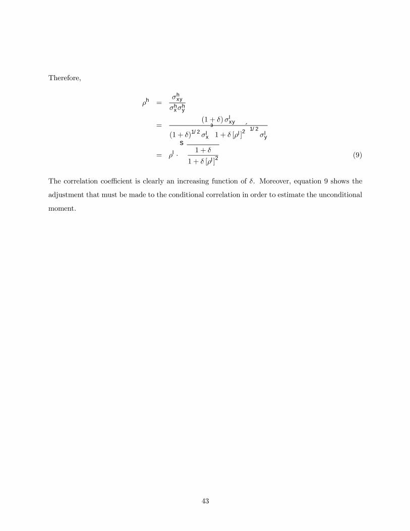
Therefore,

ρh =σh

xy

σhxσ

hy

=(1 + δ)σl

xy

(1 + δ)1/2 σlx

³1 + δ [ρl]2

´1/2σl

y

= ρl ·s

1 + δ

1 + δ [ρl]2 (9)

The correlation coefficient is clearly an increasing function of δ. Moreover, equation 9 shows the

adjustment that must be made to the conditional correlation in order to estimate the unconditional

moment.

43