arXiv:0902.1915v1 [hep-ph] 11 Feb 2009 TTP09-02 SFB/CPP-09-14 NNLO vertex corrections in charmless hadronic B decays: Real part Guido Bell 1 Institut f¨ ur Theoretische Teilchenphysik, Universit¨ at Karlsruhe, D-76128 Karlsruhe, Germany Abstract We compute the real part of the 2-loop vertex corrections for charmless hadronic B decays, completing the NNLO calculation of the topological tree amplitudes in QCD factorization. Among the technical aspects we show that the hard-scattering kernels are free of soft and collinear infrared divergences at the 2-loop level, which follows after an intricate subtraction procedure involving evanescent four quark operators. The numerical impact of the considered corrections is found to be mod- erate, whereas the factorization scale dependence of the topological tree amplitudes is significantly reduced at NNLO. We in particular do not find an enhancement of the phenomenologically important ratio |C/T | from the perturbative calculation. 1 E-mail:[email protected]

Welcome message from author
This document is posted to help you gain knowledge. Please leave a comment to let me know what you think about it! Share it to your friends and learn new things together.
Transcript
arX
iv:0
902.
1915
v1 [
hep-
ph]
11
Feb
2009
TTP09-02
SFB/CPP-09-14
NNLO vertex corrections in charmless
hadronic B decays: Real part
Guido Bell1
Institut fur Theoretische Teilchenphysik,
Universitat Karlsruhe, D-76128 Karlsruhe, Germany
Abstract
We compute the real part of the 2-loop vertex corrections for charmless hadronic
B decays, completing the NNLO calculation of the topological tree amplitudes in
QCD factorization. Among the technical aspects we show that the hard-scattering
kernels are free of soft and collinear infrared divergences at the 2-loop level, which
follows after an intricate subtraction procedure involving evanescent four quark
operators. The numerical impact of the considered corrections is found to be mod-
erate, whereas the factorization scale dependence of the topological tree amplitudes
is significantly reduced at NNLO. We in particular do not find an enhancement of
the phenomenologically important ratio |C/T | from the perturbative calculation.
1E-mail:[email protected]
1 Introduction
The study of hadronic B meson decays into a pair of light (charmless) mesons reveals
interesting information about the underlying four quark interactions and the related phe-
nomenon of CP violation. While these decay modes are intensively investigated at current
and future B physics experiments, the main challenge for precise theoretical predictions
consists in the computation of the hadronic matrix elements. QCD factorization [1], or
its field theoretical formulation in the language of Soft-Collinear Effective Theory [2],
is a systematic framework to compute these matrix elements from first principles. The
starting point is a factorization formula, which holds in the heavy quark limit mb → ∞,
〈M1M2|Qi|B〉 ≃ FBM1+ (0) fM2
∫
du T Ii (u) φM2(u)
+ fB fM1 fM2
∫
dωdvdu T IIi (ω, v, u) φB(ω) φM1(v) φM2(u), (1)
where the perturbatively calculable hard-scattering kernels T I,IIi encode the short-distance
strong-interaction effects and the non-perturbative physics is confined to some process-
independent hadronic parameters such as decay constants fM , light-cone distribution
amplitudes φM and a transition form factor FBM1+ at maximum recoil q2 = 0.
In this work we address perturbative corrections to the factorization formula (1).
Whereas next-to-leading order (NLO) corrections to the hard-scattering kernels T I,IIi are
known from the pioneering work in [1], partial next-to-next-to-leading order (NNLO)
corrections have recently been worked out [3, 4, 5, 6]. The α2s corrections to the kernels
T IIi (spectator scattering) are by now completely determined to NNLO: the corrections for
the topological tree amplitudes have been computed in [3] and the ones for the so-called
penguin amplitudes in [4].
In contrast to this the computation of α2s corrections to the kernels T I
i (vertex cor-
rections) is to date incomplete. Whereas we computed the imaginary parts of the hard-
scattering kernels for the topological tree amplitudes in [5, 6], we complete the NNLO
calculation of the tree amplitudes in this work by computing the respective real parts.
Partial results of this calculation, in particular the analytical expressions of the required
2-loop Master Integrals, have already been given in [6].
The organization of this paper is as follows: The technical aspects of the NNLO
calculation are presented in Section 2. We start by briefly recalling our definitions and
conventions and make some remarks concerning the computation of the 2-loop diagrams.
We then show in some detail how to extract the hard-scattering kernels from the matrix
elements which are formally infrared divergent. This subtraction procedure, which be-
comes particularly involved for the colour-suppressed tree amplitude, is complicated due
to the presence of evanescent four quark operators which arise in intermediate steps of
the calculation. Our analytical results for the hard-scattering kernels are summarized in
Section 3. We briefly discuss the numerical impact of the considered NNLO corrections
in Section 4, before we conclude in Section 5. Several technical issues of the calculation
and the explicit expressions of the hard-scattering kernels are relegated to the Appendix.
1
2 NNLO calculation
The calculation of the real parts of the topological tree amplitudes proceeds along the
same lines as the one of the imaginary parts that we presented in [5]. Still, the current
calculation turns out to be considerably more complex in several respects. First, it
requires the calculation of a larger amount of 2-loop integrals, which are in addition
more complicated since they involve up to three (instead of one) massive propagators.
Second, the renormalization procedure and the infrared subtractions reveal their full 2-
loop complexity only in the current calculation as a consequence of the fact that the
tree level contribution is real. In the following we summarize the technical aspects of
the calculation and refer for a more detailed description of the general strategy to [5]
(cf. also [6]).
2.1 Operator basis
The topological tree amplitudes can be derived from the hadronic matrix elements of the
current-current operators in the effective weak Hamiltonian
Heff =GF√2V ∗udVub (C1Q1 + C2Q2) + h.c. (2)
As we apply Dimensional Regularization1 (DR) to regularize ultraviolet (UV) and infrared
(IR) singularities, evanescent four-quark operators appear in intermediate steps of the
calculation. The full operator basis required for the present calculation becomes2
Q1 =[
uγµLTAb] [
dγµLTAu]
,
Q2 = [uγµL b][
dγµLu]
,
E1 =[
uγµγνγρLTAb] [
dγµγνγρLTAu]
− 16Q1,
E2 = [uγµγνγρL b][
dγµγνγρLu]
− 16Q2,
E ′1 =
[
uγµγνγργσγτLTAb] [
dγµγνγργσγτ LTAu]
− 20E1 − 256Q1,
E ′2 = [uγµγνγργσγτL b]
[
dγµγνγργσγτ Lu]
− 20E2 − 256Q2, (3)
with colour matrices TA and L = 1 − γ5. We stress that previous studies within QCD
factorization, as e.g. [1, 3, 4], have often been formulated in a different operator basis
with a Fierz-symmetric definition of the physical operators. As has been argued in [5], it
is more convenient for the current calculation to use the operator basis (3) since it allows
to work with a naive anticommuting γ5 beyond NLO [7].
There are two different insertions of a four-quark operator which are illustrated in
Figure 1 of [5]. The first one gives rise to the colour-allowed tree amplitude α1(M1M2),
which corresponds to the flavour content [qsb] of the decaying B meson, [qsu] of the recoil
1We write d = 4− 2ε and use an anticommuting γ5 according to the NDR scheme.2This operator basis has been named CMM basis in [5] (denoted by a hat).
2
meson M1 and [ud] of the emitted meson M2. The colour-suppressed tree amplitude
α2(M1M2) follows from the second insertion and belongs to the flavour contents [qsb],
[qsd] and [uu], respectively. In [5] we did not consider the second type of insertions since
we could derive the imaginary part of the colour-suppressed amplitude from the one of
the colour-allowed amplitude using Fierz-symmetry arguments3.
In the current calculation we cannot proceed along the same lines, since a Fierz-
symmetric operator basis has not yet been worked out to NNLO4. We therefore consider
both types of insertions in this work, which also provides an independent cross-check of
our previous result for the imaginary part of the colour-suppressed tree amplitude.
2.2 2-loop calculation
The main task of the calculation consists in the computation of a large number of 2-loop
diagrams (shown in Figure 2 of [5]). We use an automatized reduction algorithm, which
is based on integration-by-parts techniques [11], to express these diagrams in terms of an
irreducible set of Master Integrals (MIs). In addition to the MIs that appeared in the
calculation of the imaginary part of the NNLO vertex corrections (cf. Figure 3 of [5]), we
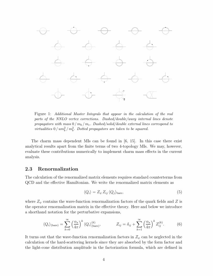
find 22 MIs which are shown in Figure 1. In total the current calculation requires the
computation of 36 MIs to up to five orders in the ε-expansion.
Apart from the MIs that involve the charm quark mass, the analytical results for the
MIs from Figure 1 can be found in [6]5. The MIs can be expressed in terms of Harmonic
Polylogarithms (HPLs) [14] of weight w ≤ 4,
H(0; x) = ln(x), H(0, 0, 1; x) = Li3(x),
H(1; x) = − ln(1− x), H(0, 1, 1; x) = S1,2(x),
H(−1; x) = ln(1 + x), H(0, 0, 0, 1; x) = Li4(x),
H(0, 1; x) = Li2(x), H(0, 0, 1, 1; x) = S2,2(x),
H(0,−1; x) = −Li2(−x), H(0, 1, 1, 1; x) = S1,3(x).
H(−1, 0, 1; x) ≡ H1(x), H(0,−1, 0, 1; x) ≡ H2(x), (4)
where we introduced a shorthand notation for the last two HPLs6. Moreover, the massive
non-planar 6-topology MI (last diagram from Figure 1) involves a constant in the finite
term which, until recently, was only known numerically, C0 = −60.2493267(10) [13]. In a
recent work it was shown that its analytical value is C0 = −167π4/270 [16].
3To do so we introduced a second operator basis named traditional basis in [5] (denoted by a tilde).4We emphasize that the operator basis from Section 8 in [8] is not Fierz-symmetric and the one from
Appendix A in [9] is presumably not either [10].5Part of these results have recently been confirmed by various groups [12, 13].6The explicit expression of H1(x) in terms of Nielsen Polylogarithms can be found e.g. in equation
(10) of [15]. On the other hand H2(x) has to be evaluated numerically (in Section 3.2 we find, however,
analytical expressions in the convolutions with the light-cone distribution amplitude of the meson M2).
3
u
2
0
Figure 1: Additional Master Integrals that appear in the calculation of the real
parts of the NNLO vertex corrections. Dashed/double/wavy internal lines denote
propagators with mass 0 /mb /mc. Dashed/solid/double external lines correspond to
virtualities 0 /um2b /m
2b . Dotted propagators are taken to be squared.
The charm mass dependent MIs can be found in [6, 15]. In this case there exist
analytical results apart from the finite terms of two 4-topology MIs. We may, however,
evaluate these contributions numerically to implement charm mass effects in the current
analysis.
2.3 Renormalization
The calculation of the renormalized matrix elements requires standard counterterms from
QCD and the effective Hamiltonian. We write the renormalized matrix elements as
〈Qi〉 = Zψ Zij 〈Qj〉bare, (5)
where Zψ contains the wave-function renormalization factors of the quark fields and Z is
the operator renormalization matrix in the effective theory. Here and below we introduce
a shorthand notation for the perturbative expansions,
〈Qi〉(bare) =∞∑
k=0
(αs4π
)k
〈Qi〉(k)(bare), Zij = δij +∞∑
k=1
(αs4π
)k
Z(k)ij . (6)
It turns out that the wave-function renormalization factors in Zψ can be neglected in the
calculation of the hard-scattering kernels since they are absorbed by the form factor and
the light-cone distribution amplitude in the factorization formula, which are defined in
4
terms of full QCD fields (rather than HQET or SCET fields), for details cf. Section 4.2
of [5]. We renormalize the coupling constant in the MS-scheme,
Z(1)g = −
(
11
6CA − 1
3nf
)
1
ε, (7)
and the b-quark mass in the on-shell scheme,
Z(1)m = −CF
(
eγEµ2
m2b
)ε
Γ(ε)3− 2ε
1− 2ε. (8)
The 1-loop and 2-loop MS operator renormalization matrices can be inferred from [8, 17]
Z(1) =
(
− 2 43
512
29
0 0
6 0 1 0 0 0
)
1
ε,
Z(2) =
(
17− 23nf −26
3+ 4
9nf −25
6+ 5
36nf −31
18+ 2
27nf
1996
5108
− 39 + 2nf 4 −314+ 1
3nf 0 5
2419
)
1
ε2
+
(
7912
+ 49nf −205
18+ 10
27nf
1531288
− 5216
nf − 172
− 181nf
1384
− 35864
834+ 5
3nf 3 119
16− 1
18nf
89
− 35192
− 772
)
1
ε, (9)
where the lines refer to the physical operators and the columns to the full operator basis
including the evanescent operators from (3).
2.4 IR subtractions
In order to extract the hard-scattering kernels Ti we rewrite the renormalized matrix
elements in the factorized form
〈Qi〉 = F · Ti ⊗ Φ + . . . (10)
where F denotes the form factor, Φ the product of decay constant and distribution
amplitude, ⊗ the convolution integral and the ellipsis the spectator scattering term which
we disregard in the following. As has been discussed in detail in Section 4.2 of [5], only
naively non-factorizable (nf) 1-loop diagrams contribute to the NLO kernels,
〈Qi〉(1)nf + Z(1)ij 〈Qj〉(0) = F (0) · T (1)
i ⊗ Φ(0). (11)
Similarly, the calculation of the NNLO kernels involves only non-factorizable 2-loop dia-
grams (but factorizable (f) 1-loop diagrams),
〈Qi〉(2)nf + Z(1)ij
[
〈Qj〉(1)nf + 〈Qj〉(1)f
]
+ Z(2)ij 〈Qj〉(0)
= F (0) · T (2)i ⊗ Φ(0) + F (1)
amp · T(1)i ⊗ Φ(0) + F (0) · T (1)
i ⊗ Φ(1)amp, (12)
5
where the subscript ”amp” (amputated) has been introduced to denote corrections with-
out wave-function renormalization. We see that the calculation of the NNLO kernels re-
quires the NLO kernels to O(ε2) as they enter (12) in combination with the IR-divergent
form factor correction F(1)amp ∼ 1/ε2IR. As a consequence the factorization formula has
to be extended in intermediate steps of the calculation to include evanescent operators,
which have to be renormalized such that their (IR-finite) matrix elements vanish (for
details cf. Section 4.3 of [5]).
At NNLO the subtraction procedure becomes somewhat involved. It is particularly
complicated in the calculation of the colour-suppressed tree amplitude, where a Fierz-
evanescent operator appears at tree level. In the following we discuss the subtraction
procedure in some detail. Throughout this section we concentrate on the real parts of
the hard-scattering kernels, since the respective imaginary parts have already been given
in [5]. We refer to Appendix A for the explicit expressions of the auxiliary coefficient
functions ti(u) that we introduce below.
Colour-allowed tree amplitude
To NNLO we find three operators that contribute to the right hand side of (10). In
the position space representation they correspond to products of a local heavy-to-light
current u(x)Γ1b(x) and a non-local light-quark current d(y)[y, x]Γ2u(x), where the usual
gauge link factor [y, x] is understood. We choose the basis of Dirac structures Γ1⊗Γ2 as7
O = [γµL]⊗ [γµL] ,
OE = [γµγνγρL]⊗ [γµγνγρL]− 16O,
OE′ = [γµγνγργσγτL]⊗ [γµγνγργσγτ L]− 20OE − 256O, (13)
such that the factorized hadronic matrix element of O gives the standard QCD form
factor and the light-cone distribution amplitude of the emitted meson M2. The operators
OE and OE′ are evanescent.
We first compute (11) to O(ε2) to determine the NLO kernels. We find that the
colour-singlet kernels vanish, T(1)2 = T
(1)2,E = T
(1)2,E′ = 0, while the colour-octet kernels
become
Re T(1)1 (u) =
CF2Nc
(
µ2
m2b
)ε{
t0(u)− 6L+(
t1(u) + 3L2)
ε+(
t2(u)− L3)
ε2 +O(ε3)
}
,
Re T(1)1,E(u) = − CF
4Nc
(
µ2
m2b
)ε{
tE,0(u) + 2L+(
tE,1(u)− L2)
ε+O(ε2)
}
, (14)
and T(1)1,E′ = 0 with L = lnµ2/m2
b . The IR subtractions on the right hand side of (12)
require in addition form factor and wave function corrections to the operators O and OE
(they can be found in Section 4.3 of [5]). We finally perform the convolutions of the NLO
7We do not consider colour-octet operators since their hadronic matrix elements vanish.
6
kernels with the wave function corrections, which yields
F (0) Re T(1)1 Φ(1)
amp =C2F
Nc
(
µ2
m2b
)ε{t3(u)
ε+ t4(u) +O(ε)
}
F (0) Φ(0) (15)
and an additional µ-dependent contribution to the physical kernel from
F(0)E Re T
(1)1,E Φ
(1)amp,E → C2
F
Nc
{
12L+ tE,2(u) +O(ε)
}
F (0) Φ(0). (16)
Colour-suppressed tree amplitude
In this case we find an analogous set of operators,
O = [γµL] ⊗ [γµL] ,
OE = [γµγνγρL] ⊗ [γµγνγρL]− 16 O,
OE′ = [γµγνγργσγτL] ⊗ [γµγνγργσγτ L]− 20 OE − 256 O, (17)
but the fields are now given in the wrong ordering u(y)[y, x]Γ1b(x) and d(x)Γ2u(x) (indi-
cated by ⊗), which does not yield a form factor and a light-cone distribution amplitude.
The latter follow from the factorized hadronic matrix element of the operator
O = d(x)γµLb(x) ⊗ u(y)[y, x]γµLu(x), (18)
which is the Fierz-symmetric counterpart of O. We therefore extend the right hand side
of (10) to include four operators in this case: the physical operator O, the evanescent
operators OE and OE′ and the Fierz-evanescent operator OF ≡ O −O.
The IR subtractions turn out to be particularly complicated in this case, due to
the fact that the evanescent operator OF already appears in the tree level calculation.
As a consequence the naive split-up into non-factorizable diagrams, which contribute to
the hard-scattering kernels, and factorizable diagrams, which give form factor and wave
function corrections, is spoiled. In NLO we find that equations (30) and (31) of [5] should
be replaced by8
〈Qi〉(1)nf + Z(1)ij 〈Qj〉(0) = F (0) · T (1)
i ⊗ Φ(0) + ∆(1)F,i,
〈Qi〉(1)f + Z(1)ψ 〈Qi〉(0) = F (1) · T (0)
i ⊗ Φ(0) + F (0) · T (0)i ⊗ Φ(1) − ∆
(1)F,i, (19)
where ∆(1)F,i contains the (non-vanishing) 1-loop counterterms of the form factor and wave
function corrections for the Fierz-evanescent operator OF . In other words, the split-up
in the above example of the colour-allowed tree amplitude followed from the fact that
the corresponding counterterms vanish for the physical operator O (i.e. ∆(k)i = 0).
From the first equation in (19) we see that we can neglect the factorizable 1-loop
diagrams in the computation of the NLO kernels. In order to account for the counterterm
8We introduce the ”hat” notation to distinguish these quantities from those of the preceding section.
7
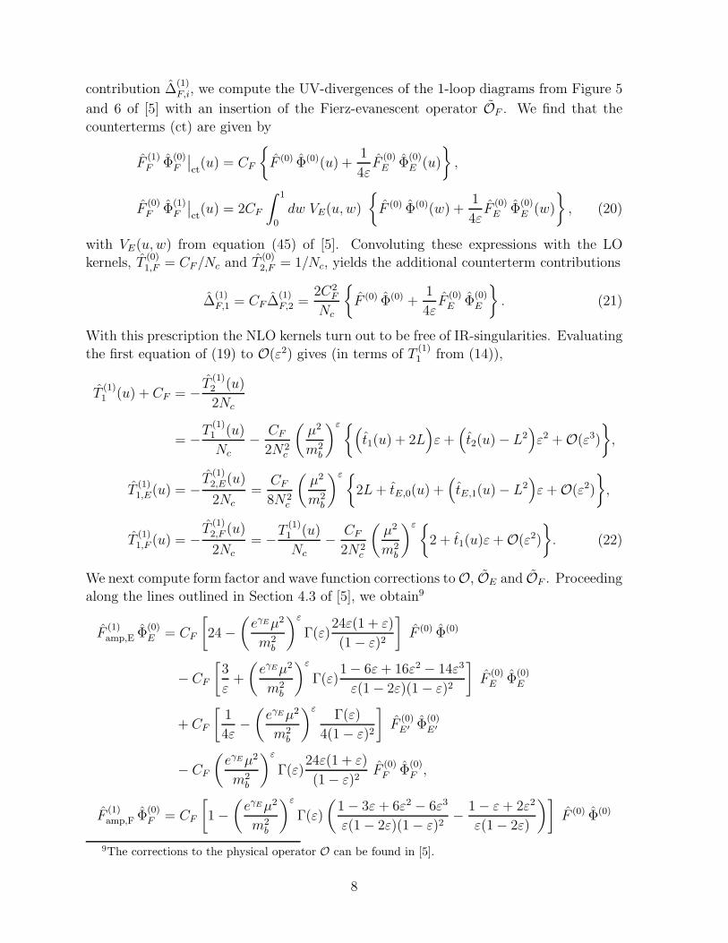
contribution ∆(1)F,i, we compute the UV-divergences of the 1-loop diagrams from Figure 5
and 6 of [5] with an insertion of the Fierz-evanescent operator OF . We find that the
counterterms (ct) are given by
F(1)F Φ
(0)F
∣
∣
ct(u) = CF
{
F (0) Φ(0)(u) +1
4εF
(0)E Φ
(0)E (u)
}
,
F(0)F Φ
(1)F
∣
∣
ct(u) = 2CF
∫ 1
0
dw VE(u, w)
{
F (0) Φ(0)(w) +1
4εF
(0)E Φ
(0)E (w)
}
, (20)
with VE(u, w) from equation (45) of [5]. Convoluting these expressions with the LO
kernels, T(0)1,F = CF/Nc and T
(0)2,F = 1/Nc, yields the additional counterterm contributions
∆(1)F,1 = CF ∆
(1)F,2 =
2C2F
Nc
{
F (0) Φ(0) +1
4εF
(0)E Φ
(0)E
}
. (21)
With this prescription the NLO kernels turn out to be free of IR-singularities. Evaluating
the first equation of (19) to O(ε2) gives (in terms of T(1)1 from (14)),
T(1)1 (u) + CF = − T
(1)2 (u)
2Nc
= −T(1)1 (u)
Nc
− CF2N2
c
(
µ2
m2b
)ε{(
t1(u) + 2L)
ε+(
t2(u)− L2)
ε2 +O(ε3)
}
,
T(1)1,E(u) = −
T(1)2,E(u)
2Nc=
CF8N2
c
(
µ2
m2b
)ε{
2L+ tE,0(u) +(
tE,1(u)− L2)
ε+O(ε2)
}
,
T(1)1,F (u) = −
T(1)2,F (u)
2Nc= −T
(1)1 (u)
Nc− CF
2N2c
(
µ2
m2b
)ε{
2 + t1(u)ε+O(ε2)
}
. (22)
We next compute form factor and wave function corrections toO, OE and OF . Proceeding
along the lines outlined in Section 4.3 of [5], we obtain9
F(1)amp,E Φ
(0)E = CF
[
24−(
eγEµ2
m2b
)ε
Γ(ε)24ε(1 + ε)
(1− ε)2
]
F (0) Φ(0)
− CF
[
3
ε+
(
eγEµ2
m2b
)ε
Γ(ε)1− 6ε+ 16ε2 − 14ε3
ε(1− 2ε)(1− ε)2
]
F(0)E Φ
(0)E
+ CF
[
1
4ε−(
eγEµ2
m2b
)εΓ(ε)
4(1− ε)2
]
F(0)E′ Φ
(0)E′
− CF
(
eγEµ2
m2b
)ε
Γ(ε)24ε(1 + ε)
(1− ε)2F
(0)F Φ
(0)F ,
F(1)amp,F Φ
(0)F = CF
[
1−(
eγEµ2
m2b
)ε
Γ(ε)
(
1− 3ε+ 6ε2 − 6ε3
ε(1− 2ε)(1− ε)2− 1− ε+ 2ε2
ε(1− 2ε)
)]
F (0) Φ(0)
9The corrections to the physical operator O can be found in [5].
8
+ CF
[
1
4ε−(
eγEµ2
m2b
)εΓ(ε)
4(1− ε)2
]
F(0)E Φ
(0)E
− CF
(
eγEµ2
m2b
)ε
Γ(ε)1− 3ε+ 6ε2 − 6ε3
ε(1− 2ε)(1− ε)2F
(0)F Φ
(0)F (23)
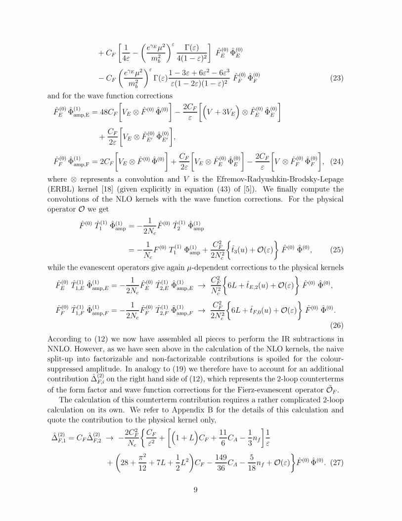
and for the wave function corrections
F(0)E Φ
(1)amp,E = 48CF
[
VE ⊗ F (0) Φ(0)
]
− 2CFε
[
(
V + 3VE
)
⊗ F(0)E Φ
(0)E
]
+CF2ε
[
VE ⊗ F(0)E′ Φ
(0)E′
]
,
F(0)F Φ
(1)amp,F = 2CF
[
VE ⊗ F (0) Φ(0)
]
+CF2ε
[
VE ⊗ F(0)E Φ
(0)E
]
− 2CFε
[
V ⊗ F(0)F Φ
(0)F
]
, (24)
where ⊗ represents a convolution and V is the Efremov-Radyushkin-Brodsky-Lepage
(ERBL) kernel [18] (given explicitly in equation (43) of [5]). We finally compute the
convolutions of the NLO kernels with the wave function corrections. For the physical
operator O we get
F (0) T(1)1 Φ(1)
amp = − 1
2NcF (0) T
(1)2 Φ(1)
amp
= − 1
Nc
F (0) T(1)1 Φ(1)
amp +C2F
2N2c
{
t3(u) +O(ε)
}
F (0) Φ(0), (25)
while the evanescent operators give again µ-dependent corrections to the physical kernels
F(0)E T
(1)1,E Φ
(1)amp,E = − 1
2NcF
(0)E T
(1)2,E Φ
(1)amp,E → C2
F
N2c
{
6L+ tE,2(u) +O(ε)
}
F (0) Φ(0),
F(0)F T
(1)1,F Φ
(1)amp,F = − 1
2NcF
(0)F T
(1)2,F Φ
(1)amp,F → C2
F
2N2c
{
6L+ tF,0(u) +O(ε)
}
F (0) Φ(0).
(26)
According to (12) we now have assembled all pieces to perform the IR subtractions in
NNLO. However, as we have seen above in the calculation of the NLO kernels, the naive
split-up into factorizable and non-factorizable contributions is spoiled for the colour-
suppressed amplitude. In analogy to (19) we therefore have to account for an additional
contribution ∆(2)F,i on the right hand side of (12), which represents the 2-loop counterterms
of the form factor and wave function corrections for the Fierz-evanescent operator OF .
The calculation of this counterterm contribution requires a rather complicated 2-loop
calculation on its own. We refer to Appendix B for the details of this calculation and
quote the contribution to the physical kernel only,
∆(2)F,1 = CF ∆
(2)F,2 → −2C2
F
Nc
{
CFε2
+
[
(
1 + L)
CF +11
6CA − 1
3nf
]
1
ε
+
(
28 +π2
12+ 7L+
1
2L2
)
CF − 149
36CA − 5
18nf +O(ε)
}
F (0) Φ(0). (27)
9

3 Vertex corrections in NNLO
As we have seen in the last section, the NNLO calculation of the hard-scattering kernels
requires a rather complex subtraction procedure of UV- and IR-divergences. The fact
that the kernels turn out to be free of any singularities represents both a non-trivial
confirmation of the factorization framework and a stringent cross-check of our calculation.
3.1 Hard-scattering kernels
In terms of the Wilson coefficients Ci of the physical operators Qi from the operator basis
(3), the topological tree amplitudes take to NNLO the form
α1(M1M2) = C2 +αs4π
CF2Nc
{
C1V(1) +
αs4π
[
C1 V(2)1 + C2 V
(2)2
]
+O(α2s)
}
+ . . .
α2(M1M2) =CFNc
C1 +C2
Nc+
αs4π
CF2Nc
{(
2C2 −C1
Nc
)
V (1) − 2CAC1
+αs4π
[(
2C2 −C1
Nc
)
V(2)1 +
(
CFNc
C1 +C2
Nc
)
V(2)2 + 2CAC2 V
(1)
+
(
8CF − 113
18CA − 5
9nf
)
CAC1
]
+O(α2s)
}
+ . . . (28)
where the ellipsis refer to the terms from spectator scattering which we disregard in
the following. In this notation the αs corrections have been expressed in terms of the
convolution
V (1) =
∫ 1
0
du(
− 6L+ g2(u) + iπg1(u))
φM2(u), (29)
where L = lnµ2/m2b and (recall that u = 1− u)
g1(u) = −3− 2 lnu+ 2 ln u,
g2(u) = −22 +3(1− 2u)
uln u+
[
2Li2(u)− ln2 u− 1− 3u
uln u− (u → u)
]
. (30)
If we transform these expressions into the Fierz-symmetric operator basis that has been
used in many previous QCD factorization analyses, we reproduce the NLO result from [1].
In NNLO we find the convolutions
V(2)1 =
∫ 1
0
du
{
(
36CF − 29CA + 2nf
)
L2
+
{
(29
3CA − 2
3nf
)
g2(u)−91
6CA − 10
3nf + CFh6(u)
+ iπ[(29
3CA − 2
3nf
)
g1(u) + CFh1(u)]
}
L
10
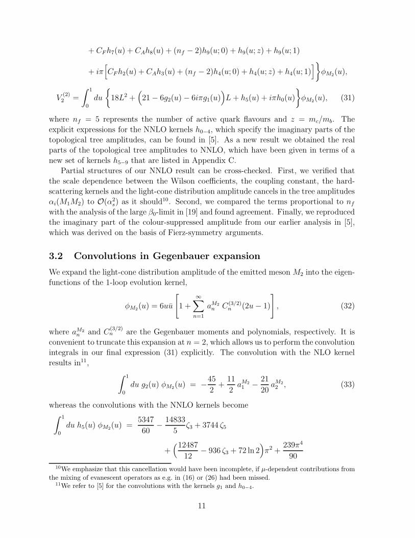
+ CFh7(u) + CAh8(u) + (nf − 2)h9(u; 0) + h9(u; z) + h9(u; 1)
+ iπ[
CFh2(u) + CAh3(u) + (nf − 2)h4(u; 0) + h4(u; z) + h4(u; 1)]
}
φM2(u),
V(2)2 =
∫ 1
0
du
{
18L2 +(
21− 6g2(u)− 6iπg1(u))
L+ h5(u) + iπh0(u)
}
φM2(u), (31)
where nf = 5 represents the number of active quark flavours and z = mc/mb. The
explicit expressions for the NNLO kernels h0−4, which specify the imaginary parts of the
topological tree amplitudes, can be found in [5]. As a new result we obtained the real
parts of the topological tree amplitudes to NNLO, which have been given in terms of a
new set of kernels h5−9 that are listed in Appendix C.
Partial structures of our NNLO result can be cross-checked. First, we verified that
the scale dependence between the Wilson coefficients, the coupling constant, the hard-
scattering kernels and the light-cone distribution amplitude cancels in the tree amplitudes
αi(M1M2) to O(α2s) as it should10. Second, we compared the terms proportional to nf
with the analysis of the large β0-limit in [19] and found agreement. Finally, we reproduced
the imaginary part of the colour-suppressed amplitude from our earlier analysis in [5],
which was derived on the basis of Fierz-symmetry arguments.
3.2 Convolutions in Gegenbauer expansion
We expand the light-cone distribution amplitude of the emitted meson M2 into the eigen-
functions of the 1-loop evolution kernel,
φM2(u) = 6uu
[
1 +∞∑
n=1
aM2n C(3/2)
n (2u− 1)
]
, (32)
where aM2n and C
(3/2)n are the Gegenbauer moments and polynomials, respectively. It is
convenient to truncate this expansion at n = 2, which allows us to perform the convolution
integrals in our final expression (31) explicitly. The convolution with the NLO kernel
results in11,
∫ 1
0
du g2(u) φM2(u) = −45
2+
11
2aM21 − 21
20aM22 , (33)
whereas the convolutions with the NNLO kernels become∫ 1
0
du h5(u) φM2(u) =5347
60− 14833
5ζ3 + 3744 ζ5
+(12487
12− 936 ζ3 + 72 ln 2
)
π2 +239π4
90
10We emphasize that this cancellation would have been incomplete, if µ-dependent contributions from
the mixing of evanescent operators as e.g. in (16) or (26) had been missed.11We refer to [5] for the convolutions with the kernels g1 and h0−4.
11
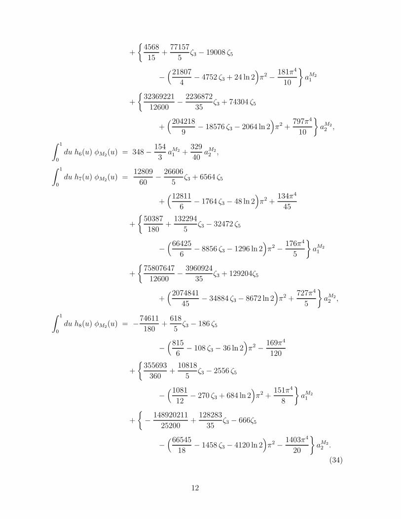
+
{
4568
15+
77157
5ζ3 − 19008 ζ5
−(21807
4− 4752 ζ3 + 24 ln 2
)
π2 − 181π4
10
}
aM21
+
{
32369221
12600− 2236872
35ζ3 + 74304 ζ5
+(204218
9− 18576 ζ3 − 2064 ln 2
)
π2 +797π4
10
}
aM22 ,
∫ 1
0
du h6(u) φM2(u) = 348− 154
3aM21 +
329
40aM22 ,
∫ 1
0
du h7(u) φM2(u) =12809
60− 26606
5ζ3 + 6564 ζ5
+(12811
6− 1764 ζ3 − 48 ln 2
)
π2 +134π4
45
+
{
50387
180+
132294
5ζ3 − 32472 ζ5
−(66425
6− 8856 ζ3 − 1296 ln 2
)
π2 − 176π4
5
}
aM21
+
{
75807647
12600− 3960924
35ζ3 + 129204ζ5
+(2074841
45− 34884 ζ3 − 8672 ln 2
)
π2 +727π4
5
}
aM22 ,
∫ 1
0
du h8(u) φM2(u) = −74611
180+
618
5ζ3 − 186 ζ5
−(815
6− 108 ζ3 − 36 ln 2
)
π2 − 169π4
120
+
{
355693
360+
10818
5ζ3 − 2556 ζ5
−(1081
12− 270 ζ3 + 684 ln 2
)
π2 +151π4
8
}
aM21
+
{
− 148920211
25200+
128283
35ζ3 − 666ζ5
−(66545
18− 1458 ζ3 − 4120 ln 2
)
π2 − 1403π4
20
}
aM22 .
(34)
12
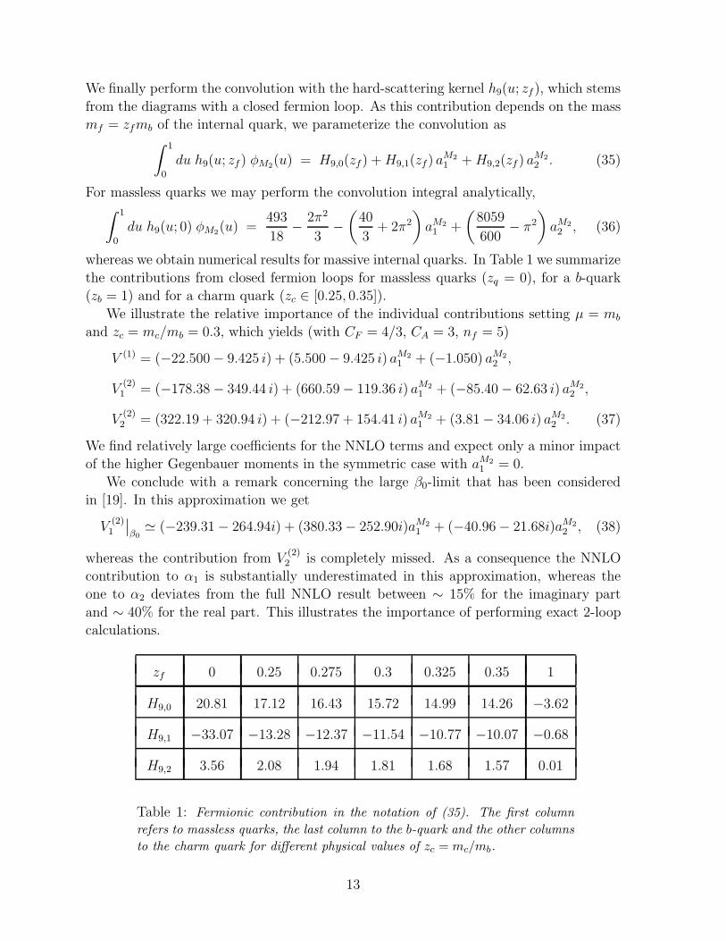
We finally perform the convolution with the hard-scattering kernel h9(u; zf), which stems
from the diagrams with a closed fermion loop. As this contribution depends on the mass
mf = zfmb of the internal quark, we parameterize the convolution as∫ 1
0
du h9(u; zf) φM2(u) = H9,0(zf ) +H9,1(zf) aM21 +H9,2(zf ) a
M22 . (35)
For massless quarks we may perform the convolution integral analytically,∫ 1
0
du h9(u; 0) φM2(u) =493
18− 2π2
3−(
40
3+ 2π2
)
aM21 +
(
8059
600− π2
)
aM22 , (36)
whereas we obtain numerical results for massive internal quarks. In Table 1 we summarize
the contributions from closed fermion loops for massless quarks (zq = 0), for a b-quark
(zb = 1) and for a charm quark (zc ∈ [0.25, 0.35]).
We illustrate the relative importance of the individual contributions setting µ = mb
and zc = mc/mb = 0.3, which yields (with CF = 4/3, CA = 3, nf = 5)
V (1) = (−22.500− 9.425 i) + (5.500− 9.425 i) aM21 + (−1.050) aM2
2 ,
V(2)1 = (−178.38− 349.44 i) + (660.59− 119.36 i) aM2
1 + (−85.40− 62.63 i) aM22 ,
V(2)2 = (322.19 + 320.94 i) + (−212.97 + 154.41 i) aM2
1 + (3.81− 34.06 i) aM22 . (37)
We find relatively large coefficients for the NNLO terms and expect only a minor impact
of the higher Gegenbauer moments in the symmetric case with aM21 = 0.
We conclude with a remark concerning the large β0-limit that has been considered
in [19]. In this approximation we get
V(2)1
∣
∣
β0≃ (−239.31− 264.94i) + (380.33− 252.90i)aM2
1 + (−40.96− 21.68i)aM22 , (38)
whereas the contribution from V(2)2 is completely missed. As a consequence the NNLO
contribution to α1 is substantially underestimated in this approximation, whereas the
one to α2 deviates from the full NNLO result between ∼ 15% for the imaginary part
and ∼ 40% for the real part. This illustrates the importance of performing exact 2-loop
calculations.
zf 0 0.25 0.275 0.3 0.325 0.35 1
H9,0 20.81 17.12 16.43 15.72 14.99 14.26 −3.62
H9,1 −33.07 −13.28 −12.37 −11.54 −10.77 −10.07 −0.68
H9,2 3.56 2.08 1.94 1.81 1.68 1.57 0.01
Table 1: Fermionic contribution in the notation of (35). The first column
refers to massless quarks, the last column to the b-quark and the other columns
to the charm quark for different physical values of zc = mc/mb.
13
4 Numerical analysis
We conclude with a brief analysis of the numerical impact of the considered NNLO cor-
rections. As a phenomenological analysis of hadronic B decays is beyond the scope of the
present paper, we focus on the perturbative structure of the topological tree amplitudes
and discuss their remnant uncertainties. In particular, we now combine our results with
the NNLO corrections from 1-loop spectator scattering that have been worked out in [3].
4.1 Implementation of spectator scattering
In contrast to the vertex corrections considered in this work, the spectator scattering
term is sensitive to two perturbative scales: the hard scale µh ∼ mb and a dynamically
generated intermediate (hard-collinear) scale µhc ∼ (ΛQCDmb)1/2. The hard scattering
kernels from spectator scattering therefore factorize further into coefficient functions HIIi ,
encoding the hard effects, and a universal hard-collinear jet-function J||. Renormaliza-
tion group techniques can be used to resum parametrically large logarithms of the form
lnmb/ΛQCD in terms of an evolution kernel U||. Following the first paper of [3], we
implement the spectator scattering contribution to the topological tree amplitudes as12
Ci(µ) T IIi (µ)⊗ [fBφB](µ)⊗ φM1(µ)⊗ φM2(µ)
→ Ci(µh) HIIi (µh)⊗ U||(µh, µhc)⊗ J||(µhc)⊗ [fBφB](µhc)⊗ φM1(µhc)⊗ φM2(µh). (39)
Since the spectator scattering starts at O(αs), the resummation is required here in
the next-to-leading-logarithmic (NLL) approximation. Unfortunately, a complete NLL
resummation is not possible since the evolution kernel U|| is known in the leading-
logarithmic (LL) approximation only [20].
We therefore proceed along the lines of our earlier analysis [5], where we worked in
the LL approximation which is consistent for the imaginary parts that are of O(α2s).
According to this, we implement the LL evolution of the HQET decay constant and the
Gegenbauer moments to evolve the hadronic parameters from their input scales to the
ones required in (39). The B meson distribution amplitude is modeled according to [21],
which implies λB(1GeV) = (0.48± 0.12)GeV and, for the first two logarithmic moments,
σ1(1GeV) = 1.6 ± 0.2 and σ2(1GeV) = 3.3 ± 0.8. The 1-loop matching corrections to
the hard functions HIIi [3] and the jet function J|| [20, 22] are implemented neglecting
crossed terms of O(α3s). We finally adopt the BBNS model from [1] to estimate the size
of power corrections to the factorization formula.
In the spectator scattering term we compute the Wilson coefficients from the effective
weak Hamiltonian in the NLL approximation with 2-loop running coupling constant.
Quantities referring to the hard scale are evaluated in a theory with nf = 5 flavours and
those referring to the hard-collinear scale with nf = 4.
12One should keep in mind that the Wilson coefficients in the spectator scattering term refer to a
different operator basis than the one used in the current work (namely the Fierz-symmetric traditional
basis that we denoted by a tilde in [5]).
14
4.2 Tree amplitudes in NNLO
We finally evaluate the topological tree amplitudes for the B → ππ channels using the
input parameters from our earlier analysis [5] and computing the Wilson coefficients
in the vertex corrections in the next-to-next-to-leading-logarithmic (NNLL) approxima-
tion [8, 23] with 3-loop running coupling constant [24] and Λ(5)MS
= 205 MeV. Under these
specifications the NNLO prediction of the topological tree amplitudes becomes13
α1(ππ) = 1.008∣
∣
V (0) +[
0.022 + 0.009i]
V (1) +[
0.024 + 0.026i]
V (2)
− 0.012∣
∣
S(1) −[
0.014 + 0.011i]
S(2) − 0.007∣
∣
P
= 1.019+0.017−0.021 + (0.025+0.019
−0.015)i,
α2(ππ) = 0.224∣
∣
V (0) −[
0.174 + 0.075i]
V (1) −[
0.030 + 0.048i]
V (2)
+ 0.075∣
∣
S(1) +[
0.032 + 0.019i]
S(2) + 0.045∣
∣
P
= 0.173+0.088−0.073 − (0.103+0.051
−0.054)i. (40)
Here we disentangled the contributions of the various terms in the factorization formula,
namely the tree level result V (0) (”naive factorization”), NLO (1-loop) vertex corrections
V (1), NNLO (2-loop) vertex corrections V (2), NLO (tree level) spectator scattering S(1),
NNLO (1-loop) spectator scattering S(2) and the modelled power corrections P .
The new contributions from this work consist in the real parts of the terms denoted by
V (2). For the colour-allowed amplitude α1(ππ), this correction is slightly larger than the
αs terms due to an numerical enhancement from the Wilson coefficients in the effective
Hamiltonian14. On the other hand, the colour-suppressed amplitude α2(ππ) receives a
13The numbers for the imaginary parts differ slightly from those of [5], since we now evaluate the
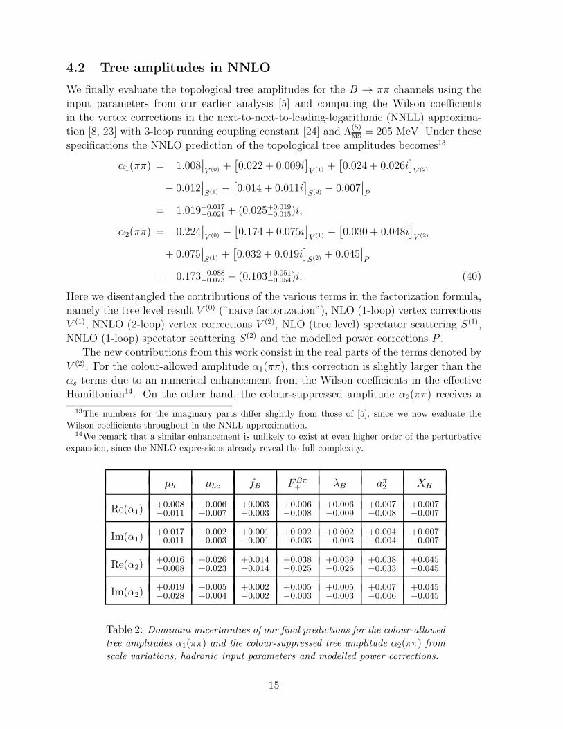
Wilson coefficients throughout in the NNLL approximation.14We remark that a similar enhancement is unlikely to exist at even higher order of the perturbative
expansion, since the NNLO expressions already reveal the full complexity.
µh µhc fB FBπ+ λB aπ2 XH
Re(α1)+0.008−0.011
+0.006−0.007
+0.003−0.003
+0.006−0.008
+0.006−0.009
+0.007−0.008
+0.007−0.007
Im(α1)+0.017−0.011
+0.002−0.003
+0.001−0.001
+0.002−0.003
+0.002−0.003
+0.004−0.004
+0.007−0.007
Re(α2)+0.016−0.008
+0.026−0.023
+0.014−0.014
+0.038−0.025
+0.039−0.026
+0.038−0.033
+0.045−0.045
Im(α2)+0.019−0.028
+0.005−0.004
+0.002−0.002
+0.005−0.003
+0.005−0.003
+0.007−0.006
+0.045−0.045
Table 2: Dominant uncertainties of our final predictions for the colour-allowed
tree amplitudes α1(ππ) and the colour-suppressed tree amplitude α2(ππ) from
scale variations, hadronic input parameters and modelled power corrections.
15
moderate correction. In particular, we do not find an enhancement of the phenomeno-
logically interesting ratio |α2/α1| from the perturbative calculation.
In Table 2 we list the uncertainties of our NNLO predictions stemming from scale
variations, hadronic input parameters and the modelled power corrections. The values
of the first two columns follow from varying the perturbative scales independently in
the ranges µh = 4.8+4.8−2.4 GeV and µhc = 1.5+0.9
−0.5 GeV. As the dependence on the hard
scale tends to cancel between vertex corrections and spectator scattering, we vary both
contributions independently and take the larger interval (from the vertex corrections) as
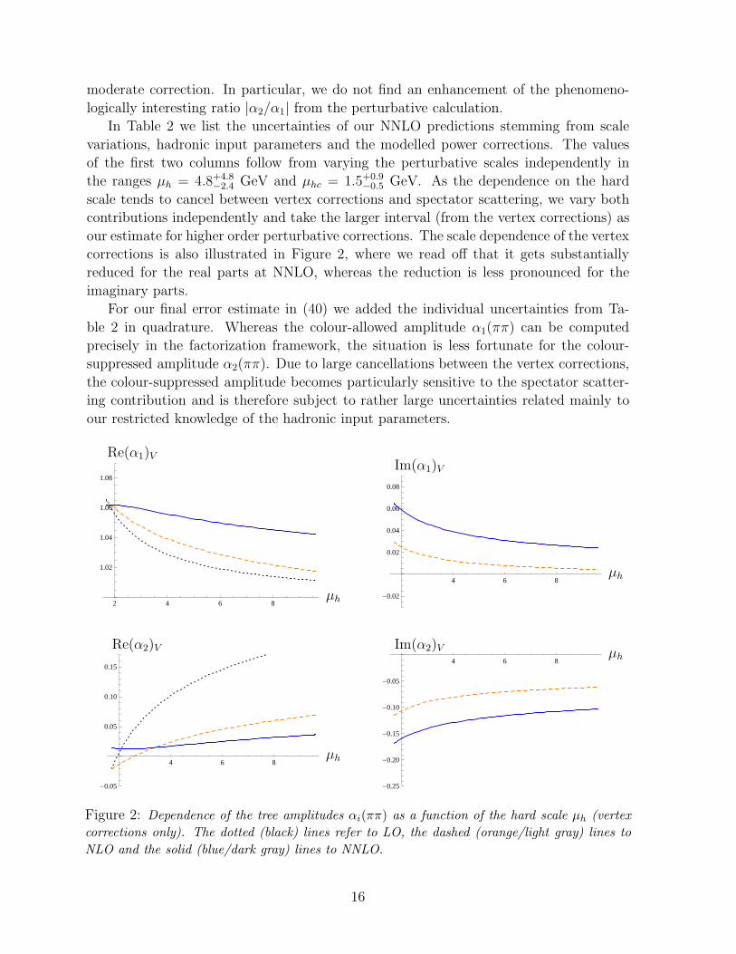
our estimate for higher order perturbative corrections. The scale dependence of the vertex
corrections is also illustrated in Figure 2, where we read off that it gets substantially
reduced for the real parts at NNLO, whereas the reduction is less pronounced for the
imaginary parts.
For our final error estimate in (40) we added the individual uncertainties from Ta-
ble 2 in quadrature. Whereas the colour-allowed amplitude α1(ππ) can be computed
precisely in the factorization framework, the situation is less fortunate for the colour-
suppressed amplitude α2(ππ). Due to large cancellations between the vertex corrections,
the colour-suppressed amplitude becomes particularly sensitive to the spectator scatter-
ing contribution and is therefore subject to rather large uncertainties related mainly to
our restricted knowledge of the hadronic input parameters.
2 4 6 8
1.02
1.04
1.06
1.08
PSfrag replacements
µh
Re(α1)V
4 6 8
-0.02
0.02
0.04
0.06
0.08
PSfrag replacements
µhRe(α1)V
µh
Im(α1)V
4 6 8
-0.05
0.05
0.10
0.15
PSfrag replacementsµh
Re(α2)V4 6 8
-0.25
-0.20
-0.15
-0.10
-0.05
PSfrag replacements
µhRe(α2)V
µhIm(α2)V
Figure 2: Dependence of the tree amplitudes αi(ππ) as a function of the hard scale µh (vertex
corrections only). The dotted (black) lines refer to LO, the dashed (orange/light gray) lines to
NLO and the solid (blue/dark gray) lines to NNLO.
16
5 Conclusion
We computed the real parts of the 2-loop vertex corrections for charmless hadronic B
meson decays, completing the NNLO calculation of the topological tree amplitudes in
the QCD factorization framework. We in particular showed how to compute the colour-
suppressed tree amplitude without making use of Fierz-symmetry arguments and found
that the hard-scattering kernels are free of IR-singularities and the resulting convolutions
with the light-cone distribution amplitude of the emitted light meson are finite, which
demonstrates factorization at the 2-loop order.
The numerical impact of the considered corrections was found to be moderate, al-
though they can be of similar size as the NLO corrections. The scale dependence of
the real parts of the topological tree amplitudes is significantly reduced at NNLO, which
allows for a precise determination of the colour-allowed amplitude α1. In contrast to this,
it remains difficult to compute the colour-suppressed amplitude α2 in the factorization
framework, since it is subject to substantial uncertainties from hadronic input parame-
ters and potential 1/mb corrections. In particular, we do not find an enhancement of the
phenomenologically important ratio |α2/α1| from the perturbative calculation.
Acknowledgements
We are grateful to Gerhard Buchalla for interesting discussions and helpful comments on
the manuscript. This work was supported by the DFG Sonderforschungsbereich/Trans-
regio 9.
A Auxiliary coefficient functions
In the calculation of the colour-allowed tree amplitude, the NLO kernels have been given
in (14) in terms of the coefficient functions
t0(u) = 4Li2(u)− ln2 u+ 2 ln u ln u+ ln2 u+ (2− 3u)( ln u
u− ln u
u
)
− π2
3− 22,
t1(u) = −2Li3(u)− 2S1,2(u)− 2 ln uLi2(u) + ln3 u− 2 ln2 u ln u+ ln u ln2 u− ln3 u
+2− 3u2
uuLi2(u)−
2− 3u
u
(
ln2 u− ln u ln u)
+6− 11u+ 2uπ2
uln u
+4− 3u
2uln2 u− 18− 33u+ 5uπ2
3uln u+
(7− 6u)π2
6u+ 2ζ3 − 52,
t2(u) = 10Li4(u)− 8S2,2(u) + 10S1,3(u)− 8 ln uLi3(u) + 10 ln u S1,2(u)−7
12ln4 u
+ 5 ln2 uLi2(u) +4
3ln3 u ln u− ln2 u ln2 u+
1
3lnu ln3 u+
7
12ln4 u
+2− 6u+ 6u2
uuLi3(u)−
4− 6u+ 3u2
uu
(
S1,2(u) + ln uLi2(u))
− 8− 3u
6uln3 u
17
+2− 3u
6u
(
4 ln3 u− 6 ln2 u ln u+ 3 lnu ln2 u)
− 60(1− 2u) + 17uπ2
12uln2 u
+3(6− 4u− 7u2) + uuπ2
3uuLi2(u) +
24− 54u+ 5uπ2
6uln u ln u+
(29− 24u)π2
6u
+6(12− 13u) + 7uπ2
12uln2 u+
24(7− 13u) + (10− 15u)π2
12uln u− 23π4
180
− 24u(7− 13u) + (2 + 23u− 27u2)π2 + 24uuζ312uu
ln u+10− 11u
uζ3 − 112,
tE,0(u) = −1− 2u
2
( ln u
u− ln u
u
)
+16
3,
tE,1(u) = −1− 2u
2uuLi2(u) +
1− 3u
4uln2 u+
u
2uln u ln u− 2− 3u
4uln2 u
− 4(1− 2u)
3
( ln u
u− ln u
u
)
− (6− 5u)π2
12u+ 12 (41)
and the convolutions of the NLO kernels with the wave function corrections, cf. (15) and
(16), involve
t3(u) = 4Li3(u) + 4S1,2(u)− 4 lnuLi2(u) +2
3ln3 u− 2 ln2 u ln u− 2
3ln3 u− Li2(u)
uu
− 1− 3u
2uu
(
u ln2 u+ 2u ln u ln u− u ln2 u)
− 3
2uln u+
(4− 3u)π2
6u− 15
2− 4ζ3,
t4(u) = 12Li4(u)− 20S2,2(u) + 12S1,3(u)− 8(
ln u+ ln u)
Li3(u) + 12 lnu S1,2(u)
+ 4 ln u S1,2(u) +(
4 ln2 u+ 4 lnu ln u+ 2 ln2 u)
Li2(u)−3
4ln4 u+
7
3ln3 u ln u
− 1
2ln2 u ln2 u− 1
3ln u ln3 u+
3
4ln4 u− 4− 11u+ 3u2
uuLi3(u) +
5− 12u
6uln3 u
+1 + u− 3u2
uuS1,2(u) +
2− 10u+ 6u2
uuln uLi2(u)−
1− 5u+ 3u2
uuln uLi2(u)
+2− 10u+ 9u2
2uuln2 u ln u− 1− 2u
2uuln u ln2 u− 5− 6u
6uln3 u
− 18− 24u+ 15u2 − 10uuπ2
3uuLi2(u)−
16− 27u+ 4uπ2
4uln2 u
− 6− 36u+ 27u2 − 4uuπ2
2uuln u ln u+
3(14− 17u) + 8uπ2
12uln2 u
+8− 15u− 4π2 − 48uζ3
4uln u+
3(2− 3u)ζ3u
− 23π4
60+
(23− 17u)π2
12u
− 81− 126u+ 45u2 − (14− 22u+ 6u2)π2 − 192uuζ312uu
ln u− 137
4,
18
tE,2(u) = −6(1− 2u)
uuLi2(u)−
6
uln u ln u− 6 lnu− 6 ln u− π2
u+ 50. (42)
In the calculation of the colour-suppressed tree amplitude, the NLO kernels in (22) contain
the coefficient functions
t1(u) =u
uln u− ln u+ 8 + iπ,
t2(u) =u
u
(
Li2(u)− ln2 u+ ln u ln u+ 4 ln u)
+1
2ln2 u− 4 ln u− (3− 2u)π2
6u+ 20
+ iπ(
4− ln u)
,
tE,0(u) =u
uln u− ln u+ 6 + iπ,
tE,1(u) = − u
u
(
Li2(u) + ln2 u− 3 ln u)
+1
2ln2 u− 3 lnu+ 14− π2
2+ iπ
(
3− ln u)
(43)
and the convolutions with the NLO kernels, cf. (25) and (26), give rise to
t3(u) =π2
3− 5 +
u
uln2 u+ 2 lnu ln u− ln2 u− ln u
u,
tE,2(u) =1
u
(
6Li2(u) + 3u lnu− π2)
− 3(1 + u)
uln u+ 27 + 3iπ,
tF,0(u) =1
u
(
2(1 + 2u)Li2(u)− u ln2 u− 2u ln u ln u+ 3u lnu− (2 + u)π2
3
)
+u
uln2 u− 3(1 + u)
uln u+ 29 + iπ
(
3− 2u
uln u+
2u
uln u)
. (44)
B Calculation of 2-loop counterterms ∆(2)F,i
We present the calculation of the 2-loop counterterms ∆(2)F,i, that are required in the
NNLO calculation of the colour-suppressed tree amplitude as described in Section 2.4.
The counterterms receive three contributions
∆(2)F,i = T
(0)i,F ⊗
{
F(2)F Φ
(0)F + F
(1)F Φ
(1)F + F
(0)F Φ
(2)F
}
ct(45)
where ⊗ represents a convolution and ”ct” refers to the counterterm contributions of the
form factor and the wave function corrections. Notice that the wave function corrections
actually correspond to local corrections to the decay constant, as a consequence of the
fact that the tree level kernels T(0)i,F are constant (cf. also (20) and (21)).
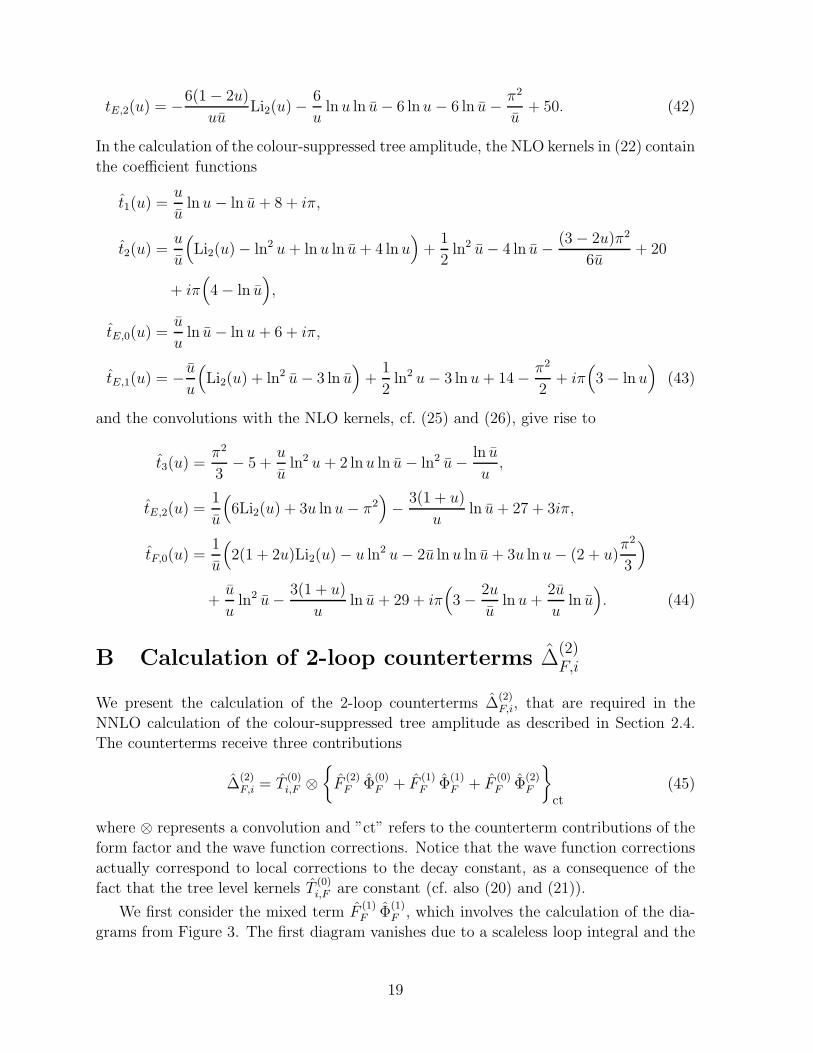
We first consider the mixed term F(1)F Φ
(1)F , which involves the calculation of the dia-
grams from Figure 3. The first diagram vanishes due to a scaleless loop integral and the
19
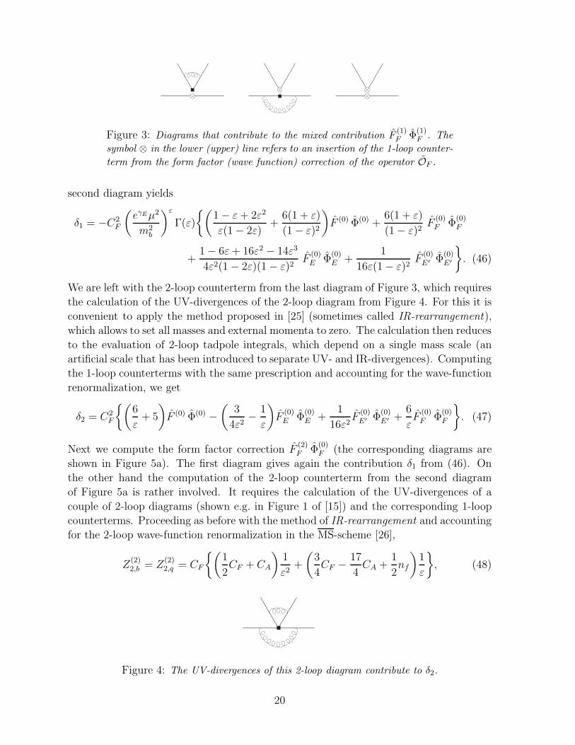
Figure 3: Diagrams that contribute to the mixed contribution F(1)F Φ
(1)F . The
symbol ⊗ in the lower (upper) line refers to an insertion of the 1-loop counter-
term from the form factor (wave function) correction of the operator OF .
second diagram yields
δ1 = −C2F
(
eγEµ2
m2b
)ε
Γ(ε)
{(
1− ε+ 2ε2
ε(1− 2ε)+
6(1 + ε)
(1− ε)2
)
F (0) Φ(0) +6(1 + ε)
(1− ε)2F
(0)F Φ
(0)F
+1− 6ε+ 16ε2 − 14ε3
4ε2(1− 2ε)(1− ε)2F
(0)E Φ
(0)E +
1
16ε(1− ε)2F
(0)E′ Φ
(0)E′
}
. (46)
We are left with the 2-loop counterterm from the last diagram of Figure 3, which requires
the calculation of the UV-divergences of the 2-loop diagram from Figure 4. For this it is
convenient to apply the method proposed in [25] (sometimes called IR-rearrangement),
which allows to set all masses and external momenta to zero. The calculation then reduces
to the evaluation of 2-loop tadpole integrals, which depend on a single mass scale (an
artificial scale that has been introduced to separate UV- and IR-divergences). Computing
the 1-loop counterterms with the same prescription and accounting for the wave-function
renormalization, we get
δ2 = C2F
{(
6
ε+ 5
)
F (0) Φ(0) −(
3
4ε2− 1
ε
)
F(0)E Φ
(0)E +
1
16ε2F
(0)E′ Φ
(0)E′ +
6
εF
(0)F Φ
(0)F
}
. (47)
Next we compute the form factor correction F(2)F Φ
(0)F (the corresponding diagrams are
shown in Figure 5a). The first diagram gives again the contribution δ1 from (46). On
the other hand the computation of the 2-loop counterterm from the second diagram
of Figure 5a is rather involved. It requires the calculation of the UV-divergences of a
couple of 2-loop diagrams (shown e.g. in Figure 1 of [15]) and the corresponding 1-loop
counterterms. Proceeding as before with the method of IR-rearrangement and accounting
for the 2-loop wave-function renormalization in the MS-scheme [26],
Z(2)2,b = Z
(2)2,q = CF
{(
1
2CF + CA
)
1
ε2+
(
3
4CF − 17
4CA +
1
2nf
)
1
ε
}
, (48)
Figure 4: The UV-divergences of this 2-loop diagram contribute to δ2.
20
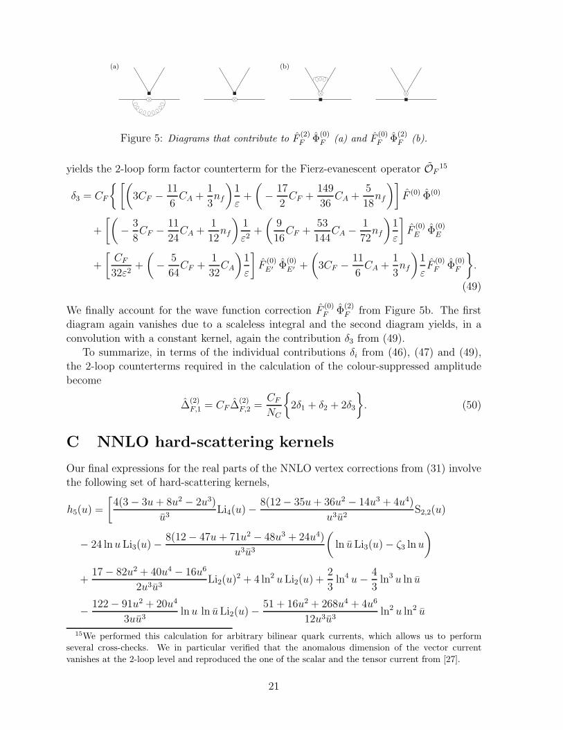
(a) (b)
Figure 5: Diagrams that contribute to F(2)F Φ
(0)F (a) and F
(0)F Φ
(2)F (b).
yields the 2-loop form factor counterterm for the Fierz-evanescent operator OF15
δ3 = CF
{[(
3CF − 11
6CA +
1
3nf
)
1
ε+
(
− 17
2CF +
149
36CA +
5
18nf
)]
F (0) Φ(0)
+
[(
− 3
8CF − 11
24CA +
1
12nf
)
1
ε2+
(
9
16CF +
53
144CA − 1
72nf
)
1
ε
]
F(0)E Φ
(0)E
+
[
CF32ε2
+
(
− 5
64CF +
1
32CA
)
1
ε
]
F(0)E′ Φ
(0)E′ +
(
3CF − 11
6CA +
1
3nf
)
1
εF
(0)F Φ
(0)F
}
.
(49)
We finally account for the wave function correction F(0)F Φ
(2)F from Figure 5b. The first
diagram again vanishes due to a scaleless integral and the second diagram yields, in a
convolution with a constant kernel, again the contribution δ3 from (49).
To summarize, in terms of the individual contributions δi from (46), (47) and (49),
the 2-loop counterterms required in the calculation of the colour-suppressed amplitude
become
∆(2)F,1 = CF ∆
(2)F,2 =
CFNC
{
2δ1 + δ2 + 2δ3
}
. (50)
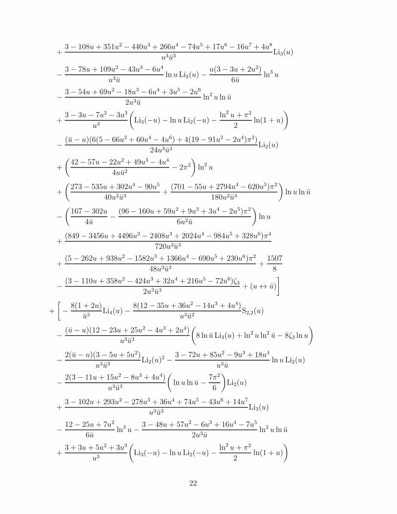
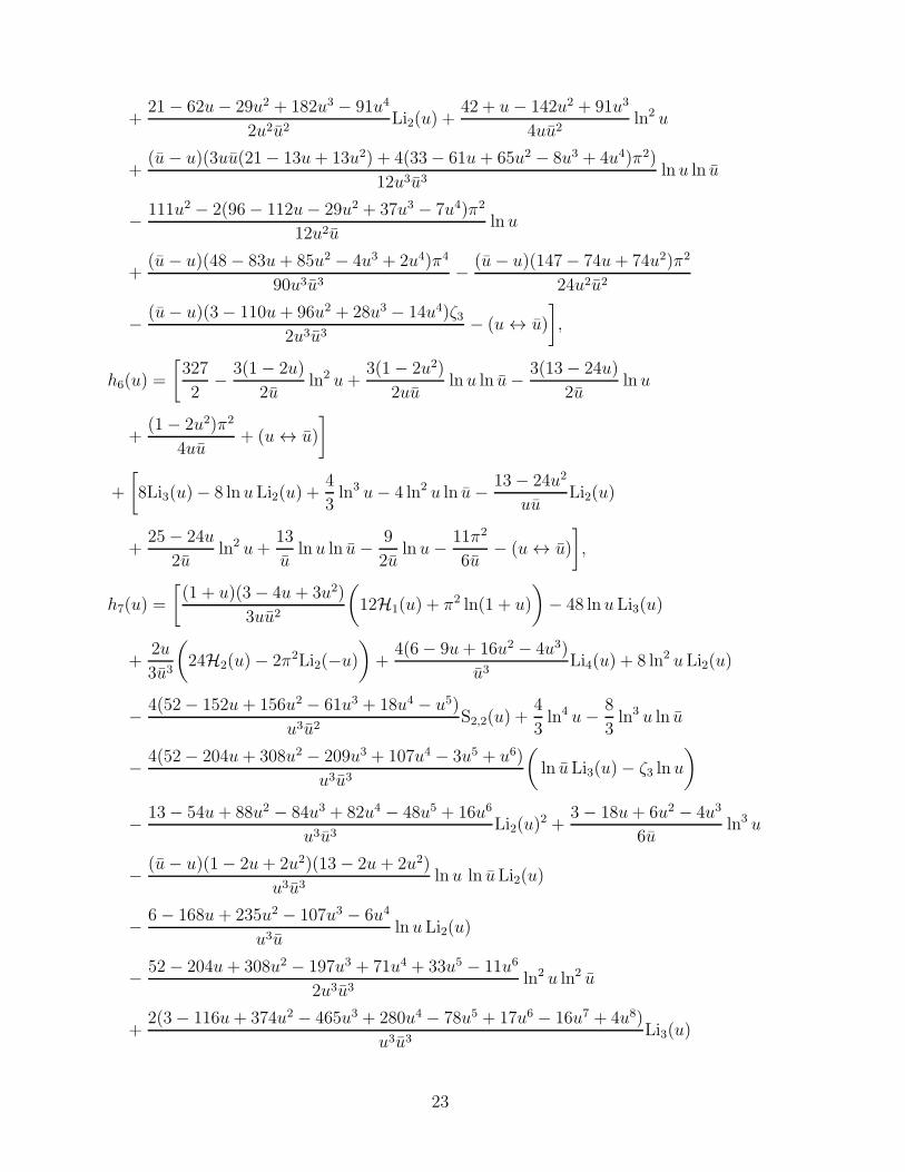
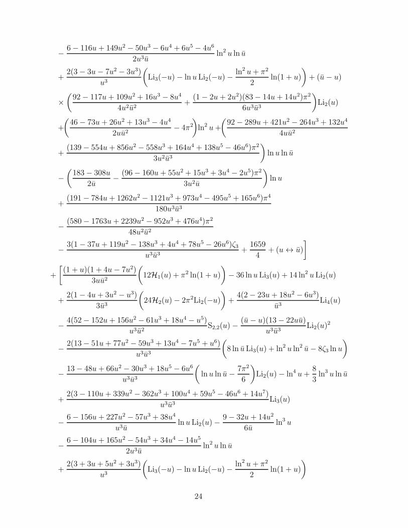
C NNLO hard-scattering kernels
Our final expressions for the real parts of the NNLO vertex corrections from (31) involve
the following set of hard-scattering kernels,
h5(u) =
[
4(3− 3u+ 8u2 − 2u3)
u3Li4(u)−
8(12− 35u+ 36u2 − 14u3 + 4u4)
u3u2S2,2(u)
− 24 lnuLi3(u)−8(12− 47u+ 71u2 − 48u3 + 24u4)
u3u3
(
ln uLi3(u)− ζ3 lnu
)
+17− 82u2 + 40u4 − 16u6
2u3u3Li2(u)
2 + 4 ln2 uLi2(u) +2
3ln4 u− 4
3ln3 u ln u
− 122− 91u2 + 20u4
3uu3ln u ln uLi2(u)−
51 + 16u2 + 268u4 + 4u6
12u3u3ln2 u ln2 u
15We performed this calculation for arbitrary bilinear quark currents, which allows us to perform
several cross-checks. We in particular verified that the anomalous dimension of the vector current
vanishes at the 2-loop level and reproduced the one of the scalar and the tensor current from [27].
21
+3− 108u+ 351u2 − 440u3 + 266u4 − 74u5 + 17u6 − 16u7 + 4u8
u3u3Li3(u)
− 3− 78u+ 109u2 − 43u3 − 6u4
u3uln uLi2(u)−
u(3− 3u+ 2u2)
6uln3 u
− 3− 54u+ 69u2 − 18u3 − 6u4 + 3u5 − 2u6
2u3uln2 u ln u
+3− 3u− 7u2 − 3u3
u3
(
Li3(−u)− lnuLi2(−u)− ln2 u+ π2
2ln(1 + u)
)
− (u− u)(6(5− 66u2 + 60u4 − 4u6) + 4(19− 91u2 − 2u4)π2)
24u3u3Li2(u)
+
(
42− 57u− 22u2 + 49u3 − 4u4
4uu2− 2π2
)
ln2 u
+
(
273− 535u+ 302u4 − 90u5
40u2u3+
(701− 55u+ 2794u4 − 620u5)π2
180u2u3
)
ln u ln u
−(
167− 302u
4u− (96− 160u+ 59u2 + 9u3 + 3u4 − 2u5)π2
6u2u
)
ln u
+(849− 3456u+ 4496u2 − 2408u3 + 2024u4 − 984u5 + 328u6)π4
720u3u3
+(5− 262u+ 938u2 − 1582u3 + 1366u4 − 690u5 + 230u6)π2
48u3u3+
1507
8
− (3− 110u+ 358u2 − 424u3 + 32u4 + 216u5 − 72u6)ζ32u3u3
+ (u ↔ u)
]
+
[
− 8(1 + 2u)
u3Li4(u)−
8(12− 35u+ 36u2 − 14u3 + 4u4)
u3u2S2,2(u)
− (u− u)(12− 23u+ 25u2 − 4u3 + 2u4)
u3u3
(
8 ln uLi3(u) + ln2 u ln2 u− 8ζ3 ln u
)
− 2(u− u)(3− 5u+ 5u2)
u3u3Li2(u)
2 − 3− 72u+ 85u2 − 9u3 + 18u4
u3uln uLi2(u)
− 2(3− 11u+ 15u2 − 8u3 + 4u4)
u3u3
(
ln u ln u− 7π2
6
)
Li2(u)
+3− 102u+ 293u2 − 278u3 + 36u4 + 74u5 − 43u6 + 14u7
u3u3Li3(u)
− 12− 25u+ 7u2
6uln3 u− 3− 48u+ 57u2 − 6u3 + 16u4 − 7u5
2u3uln2 u ln u
+3 + 3u+ 5u2 + 3u3
u3
(
Li3(−u)− ln uLi2(−u)− ln2 u+ π2
2ln(1 + u)
)
22
+21− 62u− 29u2 + 182u3 − 91u4
2u2u2Li2(u) +
42 + u− 142u2 + 91u3
4uu2ln2 u
+(u− u)(3uu(21− 13u+ 13u2) + 4(33− 61u+ 65u2 − 8u3 + 4u4)π2)
12u3u3ln u ln u
− 111u2 − 2(96− 112u− 29u2 + 37u3 − 7u4)π2
12u2uln u
+(u− u)(48− 83u+ 85u2 − 4u3 + 2u4)π4
90u3u3− (u− u)(147− 74u+ 74u2)π2
24u2u2
− (u− u)(3− 110u+ 96u2 + 28u3 − 14u4)ζ32u3u3
− (u ↔ u)
]
,
h6(u) =
[
327
2− 3(1− 2u)
2uln2 u+
3(1− 2u2)
2uuln u ln u− 3(13− 24u)
2uln u
+(1− 2u2)π2
4uu+ (u ↔ u)
]
+
[
8Li3(u)− 8 lnuLi2(u) +4
3ln3 u− 4 ln2 u ln u− 13− 24u2
uuLi2(u)
+25− 24u
2uln2 u+
13
uln u ln u− 9
2uln u− 11π2
6u− (u ↔ u)
]
,
h7(u) =
[
(1 + u)(3− 4u+ 3u2)
3uu2
(
12H1(u) + π2 ln(1 + u)
)
− 48 lnuLi3(u)
+2u
3u3
(
24H2(u)− 2π2Li2(−u)
)
+4(6− 9u+ 16u2 − 4u3)
u3Li4(u) + 8 ln2 uLi2(u)
− 4(52− 152u+ 156u2 − 61u3 + 18u4 − u5)
u3u2S2,2(u) +
4
3ln4 u− 8
3ln3 u ln u
− 4(52− 204u+ 308u2 − 209u3 + 107u4 − 3u5 + u6)
u3u3
(
ln uLi3(u)− ζ3 ln u
)
− 13− 54u+ 88u2 − 84u3 + 82u4 − 48u5 + 16u6
u3u3Li2(u)
2 +3− 18u+ 6u2 − 4u3
6uln3 u
− (u− u)(1− 2u+ 2u2)(13− 2u+ 2u2)
u3u3ln u ln uLi2(u)
− 6− 168u+ 235u2 − 107u3 − 6u4
u3uln uLi2(u)
− 52− 204u+ 308u2 − 197u3 + 71u4 + 33u5 − 11u6
2u3u3ln2 u ln2 u
+2(3− 116u+ 374u2 − 465u3 + 280u4 − 78u5 + 17u6 − 16u7 + 4u8)
u3u3Li3(u)
23
− 6− 116u+ 149u2 − 50u3 − 6u4 + 6u5 − 4u6
2u3uln2 u ln u
+2(3− 3u− 7u2 − 3u3)
u3
(
Li3(−u)− ln uLi2(−u)− ln2 u+ π2
2ln(1 + u)
)
+ (u− u)
×(
92− 117u+ 109u2 + 16u3 − 8u4
4u2u2+
(1− 2u+ 2u2)(83− 14u+ 14u2)π2
6u3u3
)
Li2(u)
+
(
46− 73u+ 26u2 + 13u3 − 4u4
2uu2− 4π2
)
ln2 u+
(
92− 289u+ 421u2 − 264u3 + 132u4
4uu2
+(139− 554u+ 856u2 − 558u3 + 164u4 + 138u5 − 46u6)π2
3u2u3
)
ln u ln u
−(
183− 308u
2u− (96− 160u+ 55u2 + 15u3 + 3u4 − 2u5)π2
3u2u
)
ln u
+(191− 784u+ 1262u2 − 1121u3 + 973u4 − 495u5 + 165u6)π4
180u3u3
− (580− 1763u+ 2239u2 − 952u3 + 476u4)π2
48u2u2
− 3(1− 37u+ 119u2 − 138u3 + 4u4 + 78u5 − 26u6)ζ3u3u3
+1659
4+ (u ↔ u)
]
+
[
(1 + u)(1 + 4u− 7u2)
3uu2
(
12H1(u) + π2 ln(1 + u)
)
− 36 lnuLi3(u) + 14 ln2 uLi2(u)
+2(1− 4u+ 3u2 − u3)
3u3
(
24H2(u)− 2π2Li2(−u)
)
+4(2− 23u+ 18u2 − 6u3)
u3Li4(u)
− 4(52− 152u+ 156u2 − 61u3 + 18u4 − u5)
u3u2S2,2(u)−
(u− u)(13− 22uu)
u3u3Li2(u)
2
− 2(13− 51u+ 77u2 − 59u3 + 13u4 − 7u5 + u6)
u3u3
(
8 ln uLi3(u) + ln2 u ln2 u− 8ζ3 ln u
)
− 13− 48u+ 66u2 − 30u3 + 18u5 − 6u6
u3u3
(
ln u ln u− 7π2
6
)
Li2(u)− ln4 u+8
3ln3 u ln u
+2(3− 110u+ 339u2 − 362u3 + 100u4 + 59u5 − 46u6 + 14u7)
u3u3Li3(u)
− 6− 156u+ 227u2 − 57u3 + 38u4
u3uln uLi2(u)−
9− 32u+ 14u2
6uln3 u
− 6− 104u+ 165u2 − 54u3 + 34u4 − 14u5
2u3uln2 u ln u
+2(3 + 3u+ 5u2 + 3u3)
u3
(
Li3(−u)− ln uLi2(−u)− ln2 u+ π2
2ln(1 + u)
)
24
+
(
92− 381u+ 161u2 + 440u3 − 220u4
4u2u2− 4(1− 3u+ 3u2)(u+ 2u3 − u4)π2
3u3u3
)
Li2(u)
+
(
46− 47u− 62u2 + 55u3
2uu2− 4π2
3
)
ln2 u+(u− u)(13 + 169u2 − 8u3 + 4u4)π4
90u3u3
+
(
(1 + u)(246− 169u2)
4u2u2+
(87− 210u2 − 16u4)π2
3u2u3
)
ln u ln u
−(
93
6u− (96− 112u− 31u2 + 34u3 − 7u4)π2
3u2u+ 4ζ3
)
ln u
− (u− u)(580− 187u+ 187u2)π2
48u2u2+
8(u− u)π2
uuln 2
− 3(u− u)(1− 39u+ 42u2 − 6u3 + 3u4)ζ3u3u3
− (u ↔ u)
]
,
h8(u) =
[
− (1 + u)(3− 4u+ 3u2)
6uu2
(
12H1(u) + π2 ln(1 + u)
)
+ 18 lnuLi3(u)
− u
3u3
(
24H2(u)− 2π2Li2(−u)
)
− 5− 22u+ 20u2 − 6u3
u3Li4(u)− 3 ln2 uLi2(u)
+4(5− 11u+ 5u2 + 5u3 + 4u4 − u5)
u3u2S2,2(u)−
1
2ln4 u+ ln3 u ln u
+4(5− 16u+ 16u2 − u3 + 3u4 − 3u5 + u6)
u3u3
(
ln uLi3(u)− ζ3 lnu
)
+(u− u)2(5− 3u+ 9u2 − 12u3 + 6u4)
4u3u3Li2(u)
2 +3 + u− 3u2 + 2u3
6uln3 u
+(u− u)(5− 13u+ 15u2 − 4u3 + 2u4)
4u3u3ln u ln uLi2(u)
+10− 32u+ 32u2 + 7u3 − 21u4 + 21u5 − 7u6
4u3u3ln2 u ln2 u
− 6− 61u+ 157u2 − 196u3 + 134u4 − 42u5 + 32u6 − 32u7 + 8u8
2u3u3Li3(u)
+6− 39u+ 47u2 − 35u3 − 12u4
2u3uln uLi2(u)−
(4 + 35u− 254u2 + 438u3 − 219u4)π2
48u2u2
+(2− u+ u2)(3− 13u+ 5u2 + 2u3 − 4u4)
4u3uln2 u ln u
− 6− 3u− 8u2 − 3u3
2u3
(
Li3(−u)− ln uLi2(−u)− ln2 u+ π2
2ln(1 + u)
)
− (u− u)
×(
(4− 7u+ 2u2)(1− 3u− 2u2)
4u2u2+
(19− 59u+ 73u2 − 28u3 + 14u4)π2
24u3u3
)
Li2(u)
25
−(
8 + 37u− 136u2 + 115u3 − 8u4
8uu2− 3π2
2
)
ln2 u
−(
4− 3u+ 24u2 − 42u3 + 21u4
8u2u2+
(127− 590u2 + 652u4 − 128u6)π2
48u3u3
)
ln u ln u
+
(
1433− 2710u
24u− (12− 30u+ 8u2 + 11u3 + 3u4 − 2u5)π2
6u2u
)
ln u
− (23− 102u+ 176u2 − 273u3 + 449u4 − 375u5 + 125u6)π4
360u3u3
+(6− 57u+ 134u2 + 26u3 − 463u4 + 540u5 − 180u6)ζ3
4u3u3− 12641
48+ (u ↔ u)
]
+
[
− (1 + u)(1 + 4u− 7u2)
6uu2
(
12H1(u) + π2 ln(1 + u)
)
+ 2 lnuLi3(u)− 3 ln2 uLi2(u)
− 1− 4u+ 3u2 − u3
3u3
(
24H2(u)− 2π2Li2(−u)
)
+19− 44u+ 36u2 − 14u3
u3Li4(u)
+4(5− 11u+ 5u2 + 5u3 + 4u4 − u5)
u3u2S2,2(u) +
(u− u)(u+ u2)(5 + 6u− 6u2)
4u3u3Li2(u)
2
+5− 16u+ 16u2 − 5u3 − 7u4 + u5 + u6
2u3u3
(
8 ln uLi3(u) + ln2 u ln2 u− 8ζ3 ln u
)
+3− 6u2 + 36u4 − 16u6
8u3u3
(
ln u ln u− 7π2
6
)
Li2(u)−1
12ln4 u− 2
3ln3 u ln u
− (u− u)(7− 4u− 20u2 + 48u3 − 24u4)
16u3u3ln2 u ln2 u
− 18− 165u+ 237u2 + 242u3 − 702u4 + 546u5 − 278u6 + 84u7
6u3u3Li3(u)
+6− 33u+ 19u2 + 7u3 + 48u4
2u3uln uLi2(u) +
30− 42u+ 7u2
6uln3 u
+18− 69u+ 78u2 − 124u3 + 217u4 − 42u5
12u3uln2 u ln u
− 6 + 3u+ 4u2 + 3u3
2u3
(
Li3(−u)− ln uLi2(−u)− ln2 u+ π2
2ln(1 + u)
)
− (u− u)(6− 283u+ 283u2)π2
72u2u2−(
36− 312u− 1493u2 + 3610u3 − 1805u4
36u2u2
− (2− 8u+ 12u2 − 5u3 − 5u4 + 9u5 − 3u6)π2
3u3u3
)
Li2(u)−4(u− u)π2
uuln 2
−(
72 + 1703u− 3724u2 + 1805u3
72uu2+
π2
3
)
ln2 u
26
−(
(u− u)(3− 10u+ 10u2)
6u2u2− (33− 21u+ 35u2 − 28u3 + 14u4)π2
12u2u3
)
ln u ln u
+
(
1009
72u− (12 + 26u− 121u2 + 80u3 − 7u4)π2
6u2u+ 4ζ3
)
ln u
− (u− u)(429 + 84u− 1244u2 + 2320u3 − 1160u4)π4
2880u3u3
+3(u− u)(2− 21u− 4u2 + 50u3 − 25u4)ζ3
4u3u3− (u ↔ u)
]
. (51)
The definition of the functions H1,2(x) can be found in Section 2.2. The diagrams with
a closed fermion loop give for massless internal quarks
h9(u; 0) =
[
125
12+
Li2(u)
u+
1− 3u
2uln2 u+
1 + u
2uln u ln u− 17(1− 2u)
6uln u
− (1 + u)π2
12u+ (u ↔ u)
]
+
[
4
3Li3(u)−
2
3ln3 u+
4
3ln2 u ln u− 32− 29u
9uLi2(u) +
35− 29u
18uln2 u
− 1
3uln u ln u− 13 + 24uπ2
18uln u+
π2
18u− (u ↔ u)
]
, (52)
and for an internal b-quark
h9(u; 1) =
[
8
u2
(
Li3(−xb)− S1,2(−xb)− ln(1 + xb)Li2(−xb)−1
12ln3 xb
1 + xb
− 1
6ln3(1 + xb) +
π2
6ln
xb1 + xb
)
− 14− 75u2 + 60u4 + 19u6
9u3u3ln u ln u
− 2yb(6 + u)
u
(
Li2(−xb)−1
4ln2 xb
1 + xb+
1
2ln2(1 + xb) +
π2
6
)
+4u
u3Li3(u)
− 32− 204u+ 504u2 − 584u3 + 405u4 − 150u5 + 29u6
9u3u3Li2(u)−
17(u− u)
6uln u
− (40− 213u2 + 120u4 − 19u6)π2
54u3u3− 2(1− 6u2 + 6u4)ζ3
u3u3
+5(61− 50u2)
24uu+ (u ↔ u)
]
+
[
− 8(3− u2)
3u2
(
Li3(−xb)− S1,2(−xb)− ln(1 + xb)Li2(−xb)−1
12ln3 xb
1 + xb
− 1
6ln3(1 + xb) +
π2
6ln
xb1 + xb
)
+54− 103u2 + 81u4
9u2u3ln u ln u
27
+2yb(38 + 29u)
9u
(
Li2(−xb)−1
4ln2 xb
1 + xb+
1
2ln2(1 + xb) +
π2
6
)
− 4(1 + 3u2 − u3)
3u3Li3(u)−
128− 504u+ 389u2
18u2uln u
− 32− 204u+ 504u2 − 584u3 + 405u4 − 150u5 + 29u6
9u3u3Li2(u)
+(42− 49u+ 39u3)π2
54uu3+
4ζ3u2u3
+261− 325u2
9uu2− (u ↔ u)
]
, (53)
where we introduced the shorthand notation
xb =1
2(yb − 1), yb =
√
4 + u
u. (54)
We finally refrain from presenting the charm quark contribution, which is rather com-
plicated and depends on two parameterizations for the 4-topology Master Integrals that
we could not solve in a closed analytical form (cf. the discussion in [15]). We may still
evaluate these Master Integrals numerically in Section 3.2 to perform the convolution
with the light-cone distribution amplitude of the emitted meson M2.
References
[1] M. Beneke, G. Buchalla, M. Neubert and C. T. Sachrajda, Phys. Rev. Lett. 83
(1999) 1914 [arXiv:hep-ph/9905312];
M. Beneke, G. Buchalla, M. Neubert and C. T. Sachrajda, Nucl. Phys. B 591 (2000)
313 [arXiv:hep-ph/0006124];
M. Beneke, G. Buchalla, M. Neubert and C. T. Sachrajda, Nucl. Phys. B 606 (2001)
245 [arXiv:hep-ph/0104110].
[2] C. W. Bauer, S. Fleming, D. Pirjol and I. W. Stewart, Phys. Rev. D 63 (2001)
114020 [arXiv:hep-ph/0011336];
C. W. Bauer, D. Pirjol and I. W. Stewart, Phys. Rev. D 65 (2002) 054022
[arXiv:hep-ph/0109045];
M. Beneke, A. P. Chapovsky, M. Diehl and T. Feldmann, Nucl. Phys. B 643 (2002)
431 [arXiv:hep-ph/0206152].
[3] M. Beneke and S. Jager, Nucl. Phys. B 751 (2006) 160 [arXiv:hep-ph/0512351];
N. Kivel, JHEP 0705 (2007) 019 [arXiv:hep-ph/0608291];
V. Pilipp, PhD thesis, LMU Munchen, 2007, arXiv:0709.0497 [hep-ph];
V. Pilipp, Nucl. Phys. B 794 (2008) 154 [arXiv:0709.3214 [hep-ph]].
[4] M. Beneke and S. Jager, Nucl. Phys. B 768 (2007) 51 [arXiv:hep-ph/0610322];
A. Jain, I. Z. Rothstein and I. W. Stewart, arXiv:0706.3399 [hep-ph].
[5] G. Bell, Nucl. Phys. B 795 (2008) 1 [arXiv:0705.3127 [hep-ph]].
28
[6] G. Bell, PhD thesis, LMU Munchen, 2006, arXiv:0705.3133 [hep-ph].
[7] K. G. Chetyrkin, M. Misiak and M. Munz, Nucl. Phys. B 520 (1998) 279
[arXiv:hep-ph/9711280].
[8] M. Gorbahn and U. Haisch, Nucl. Phys. B 713 (2005) 291 [arXiv:hep-ph/0411071].
[9] A. J. Buras, M. Gorbahn, U. Haisch and U. Nierste, JHEP 0611 (2006) 002
[arXiv:hep-ph/0603079].
[10] M. Gorbahn, private communication.
[11] F. V. Tkachov, Phys. Lett. B 100 (1981) 65;
K. G. Chetyrkin and F. V. Tkachov, Nucl. Phys. B 192 (1981) 159.
[12] R. Bonciani and A. Ferroglia, JHEP 0811 (2008) 065 [arXiv:0809.4687 [hep-ph]];
H. M. Asatrian, C. Greub and B. D. Pecjak, Phys. Rev. D 78 (2008) 114028
[arXiv:0810.0987 [hep-ph]].
[13] M. Beneke, T. Huber and X. Q. Li, Nucl. Phys. B 811 (2009) 77 [arXiv:0810.1230
[hep-ph]].
[14] E. Remiddi and J. A. M. Vermaseren, Int. J. Mod. Phys. A 15 (2000) 725
[arXiv:hep-ph/9905237].
[15] G. Bell, Nucl. Phys. B 812 (2009) 264 [arXiv:0810.5695 [hep-ph]].
[16] T. Huber, arXiv:0901.2133 [hep-ph].
[17] P. Gambino, M. Gorbahn and U. Haisch, Nucl. Phys. B 673 (2003) 238
[arXiv:hep-ph/0306079].
[18] A. V. Efremov and A. V. Radyushkin, Phys. Lett. B 94 (1980) 245;
G. P. Lepage and S. J. Brodsky, Phys. Rev. D 22 (1980) 2157.
[19] T. Becher, M. Neubert and B. D. Pecjak, Nucl. Phys. B 619 (2001) 538
[arXiv:hep-ph/0102219];
C. N. Burrell and A. R. Williamson, Phys. Rev. D 73 (2006) 114004
[arXiv:hep-ph/0504024].
[20] R. J. Hill, T. Becher, S. J. Lee and M. Neubert, JHEP 0407 (2004) 081
[arXiv:hep-ph/0404217];
M. Beneke and D. Yang, Nucl. Phys. B 736 (2006) 34 [arXiv:hep-ph/0508250].
[21] S. J. Lee and M. Neubert, Phys. Rev. D 72 (2005) 094028 [arXiv:hep-ph/0509350].
[22] T. Becher and R. J. Hill, JHEP 0410 (2004) 055 [arXiv:hep-ph/0408344];
G. G. Kirilin, arXiv:hep-ph/0508235.
29
[23] C. Bobeth, M. Misiak and J. Urban, Nucl. Phys. B 574 (2000) 291
[arXiv:hep-ph/9910220].
[24] O. V. Tarasov, A. A. Vladimirov and A. Y. Zharkov, Phys. Lett. B 93 (1980) 429;
S. A. Larin and J. A. M. Vermaseren, Phys. Lett. B 303 (1993) 334
[arXiv:hep-ph/9302208].
[25] M. Misiak and M. Munz, Phys. Lett. B 344 (1995) 308 [arXiv:hep-ph/9409454];
K. G. Chetyrkin, M. Misiak and M. Munz, Nucl. Phys. B 518 (1998) 473
[arXiv:hep-ph/9711266].
[26] E. Egorian and O. V. Tarasov, Teor. Mat. Fiz. 41 (1979) 26 [Theor. Math. Phys. 41
(1979) 863].
[27] R. Tarrach, Nucl. Phys. B 183 (1981) 384;
D. J. Broadhurst and A. G. Grozin, Phys. Rev. D 52 (1995) 4082
[arXiv:hep-ph/9410240].
30
Related Documents