H

Welcome message from author
This document is posted to help you gain knowledge. Please leave a comment to let me know what you think about it! Share it to your friends and learn new things together.
Transcript
H
NASA Conference Publication 3111
NineteenthNASTRAN o
Users'Colloquium
Computer Software Management and Information Center
University of GeorgiaAthens, Georgia
Proceedings of a colloquium held in
Williamsburg, Virginia
April 22-26, 1991
N/kSANational Aeronautics and
Space Administration
Office of Management
Scientific and TechnicalInformation Division
1991

FOREWORD
NASTRAN® (NASA STRUCTURAL ANALYSIS) is a large, comprehensive,nonproprietary, general purpose finite element computer code for structuralanalysis which was developed under NASA sponsorship and became available tothe public in late 1970. It can be obtained through COSMIC® (ComputerSoftware Management and Information Center), Athens, Georgia, and is widelyused by NASA, other government agencies, and industry.
NASA currently provides continuing maintenance of NASTRAN through COSMIC.Because of the widespread interest in NASTRAN, and finite element methods ingeneral, the Nineteenth NASTRAN Users' Colloquium was organized and held atthe Fort Magruder Inn and Conference Center, Williamsburg, Virginia on April22-26, 1991. (Papers from previous colloquia held in 1971, 1972, 1973, 1975,1976, 1977, 1978, 1979, 1980, 1982, 1983, 1984, 1985, 1986, 1987, 1988, 1989and 1990 are published in NASA Technical Memorandums X-2378, X-2637, X-2893,X-3278, X-3428, and NASA Conference Publications 2018, 2062, 2131, 2151, 2249,2284, 2328, 2373, 2419, 2481, 2505, 3029 and 3069.) The Nineteenth Colloquiumprovides some comprehensive general papers on the application of finiteelement methods in engineering, comparisons with other approaches, uniqueapplications, pre- and post-processing or auxiliary programs, and new methodsof analysis with NASTRAN.
Individuals actively engaged in the use of finite elements or NASTRANwere invited to prepare papers for presentation at the Colloquium. Thesepapers are included in this volume. No editorial review was provided by NASAor COSMIC; however, detailed instructions were provided each author to achievereasonably consistent paper format and content. The opinions and datapresented are the sole responsibility of the authors and their respectiveorganizations.
NASTRAN® and COSMIC® are registered trademarks of the National Aeronautics andSpace Administration.
iii
PRE'CEDING PAGE BLANK NOT FILMED

CONTENTS
FOREWORD ...............................
• IMPROVED NASTRAN PLOTTING .by Gordon C. Chan
(UNISYS Corporation)
o ONLINE NASTRAN DOCUMENTATION ..................
by Horace Q. Turner and David F. Harper(UNISYS Corporation)
• EXPERIENCES IN PORTING NASTRAN TO NON-TRADITIONAL PLATFORMS
by Gregory L. Davis and Robert L. Norton(Jet Propulsion Laboratory)
e MODELING OF CONNECTIONS BETWEEN SUBSTRUCTURES ..........
by Thomas G. Butler(Butler Analyses)
1 MODELING A BALL SCREW/BALL NUT IN SUBSTRUCTURING ........by Thomas G. Butler
(Butler Analyses)
o NASTRAN GPWG TABLES FOR COMBINED SUBSTRUCTURES .........by Tom Allen
(McDonnell Douglas Space Systems Co.)
e MODELING AN ELECTRIC MOTOR IN 1-D ................by Thomas G. Butler
(Butler Analyses)
= COMPUTER ANIMATION OF NASTRAN DISPLACEMENTS ON IRIS 4D-SERIESWORKSTATIONS: CANDI/ANIMATE POSTPROCESSING OF NASHUA RESULTSby Janine L. Fales
(Los Alamos National Laboratory)
o DISTILLATION TRAY STRUCTURAL PARAMETER STUDY: PHASE I ......by J. Ronald Winter
(Tennessee Eastman Company)
i0. EXPERIENCES WITH THE USE OF AXISYMMETRIC ELEMENTS IN COSMICNASTRAN FOR STATIC ANALYSIS ...................by Michael J. Cooper and William C. Walton
(Dynamic Engineering Incorporated)
11. FINITE ELEMENT SOLUTION OF TRANSIENT FLUID-STRUCTURE INTERACTIONPROBLEMS ............................by Gordon C. Everstine, Raymond S. Cheng, and Stephen A. Hambric
(David Taylor Research Center
Page
iii
I
I0
14
22
44
51
66
76
87
119
162
PRECEDING PAGE BLANK NOT FILMED
CONTENTS(Continued)
12.
13.
THE USE OF THE PLANE WAVE FLUID-STRUCTURE INTERACTION LOADINGAPPROXIMATION IN NASTRAN ....................by R. L. Dawson
(David Taylor Research Center)
SENSITIVITY ANALYSIS AND OPTIMIZATION ISSUES IN NASTRAN .....
by V, A, Tischler and V. B. Venkayya(Wright Research and Development Center)
Page
174
187
vi
N91-20507IMPROVED NASTRAN PLOTFING _, J_'_ ," _-',/
by _/
Gordon C. Chan
Unisys CorporationHuntsville, Alabama
INTRODUCTION
The graphic department of NASTRAN has received few changes since Level 17.5(1980). Only hidden line and shrink plots were added in 1983 and 1985 respectively. Anattempt to straighten tip the FIND and NOFIND options in 1985 was not very successful.Color was also added about the same time. However, the basic plotting mechanism and thestructure of the plot file remain unchanged, and they are biased towards CDC andUNIVAC machines. The plot commands were built on the technology of six bits per bytethat make the 8-bit/byte machine very awkward to use. The new 1091COSMIC/NASTRAN version, downward compatible with the older versions, tries toremove some of the old constraints, and make it easier to extract infl)rrnation from the plotfile. It also includes some useful improvements and new enhancements. ]'he new featuresavailable in the 1991 version include:
1. New PLT1 tape with simplified ASCII plot commands and short records.2. Combined hidden and shrunk plot.3. An x-y-z coordinate system on all structural plots.4. Element offset plot.5. Improved character size control.6. Improved FIND and NOFIND logic.7. A new NASTPLOT post-processor to perform screen plotting or generate
PostScript files.8. A BASIC/NASTPLOT program for PC.
PLT1/PLT2 FILE
Since Level 17.5 through the 1990 version, all the plotting goes to a PLT2 file whichis described as the "general plotter tape". The structure of the plot commands in the PLT2file is fully described in the user's and programmer's manuals. The commands, originallydesigned to be used for all machines with 32-, 36- or 60-bit computer words, wereconstructed based on 6 bits per byte structure. However, for IBM, VAX, and others, whichare using 8-bits/byte word architecture, the 6 bits per byte technology has long beenabandoned, leaving the manuals inaccurate and misleading. To use the PET2 file forgraphic plotting, a user needs to write an external program to interpret those NASTRANgenerated plot commands, and to drive his particular plotter, if such a program is notalready available. Normally this involves heavy bit and byte manipulation and datareconstruction. A disadvantage to the user is that the original bit and byte data on thePLT2 file cannot be printed to assist in debugging of his program.
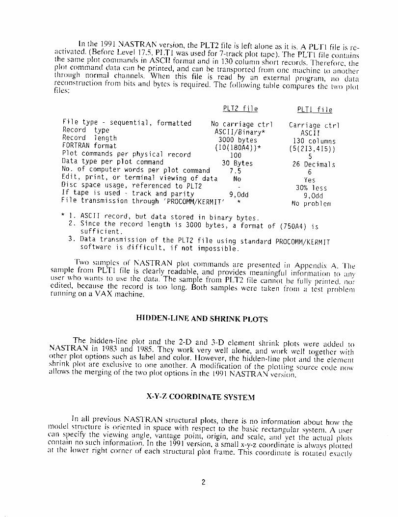
In the 1991 NASTRAN version, the PLT2 file is left alone as it is. A PLT1 file is re-
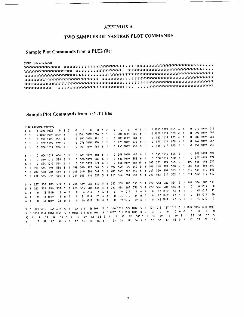
activated. (Before Level 17.5, PLT1 was used for 7-track plot tape). Tile PLT1 file containsthe same plot commands in ASCII format and in 130 column short records. Therefore, theplot command data can be printed, and can be transported from one machine to anotherthrough normal channels. When this file is read by an external program, no datareconstruction from bits and bytes is required. The following table compares the two plotfiles:
PLT2 file PLTI file
File type - sequential, formatted No carriage ctrl Carriage ctrlRecord type ASCll/Binary* ASCIIRecord length 3000 bytes 130 columnsFORTRAN format (I0(180A4))* (5(213,415))Plot commands per physical record I00 5Data type per plot command 30 Bytes 26 DecimalsNo. of computer words per plot command 7.5 6Edit, print, or terminal viewing of data No YesDisc space usage, referenced to PLT2 30% lessIf tape is used track and parity 9,Odd 9,OddFile transmission through 'PROCOMM/KERMIT' * No problem
I. ASCII record, but data stored in binary bytes.2. Since the record length is 3000 bytes, a format of (750A4) is
sufficient.3. Data transmission of the PLT2 file using standard PROCOMM/KERMIT
software is difficult, if not impossible.
Two samples of NASTRAN plot commands are presented in At)pendix A. Thesample from PLT1 file is clearly readable, and provides meaningful information to anyuser who wants to use the data. The sample from PLT2 file cannot be fully printed, noredited, because the record is too long. Both samples were taken from a test problemrunning on a VAX machine.
HIDDEN-LINE AND SHRINK PLOTS
The hidden-line plot and the 2-D and 3-D element shrink plots were added toNASTRAN in 1983 and 1985. They work very well alone, and work well together withother plot options such as label and color. However, the hidden-line plot and the elementshrink plot are exclusive to one another. A modification of the plotting source code nowallows the merging of the two plot options in the 1991 NASTRAN version.
X-Y-Z COORDINATE SYSTEM
In all previous NASTRAN structural plots, there is no information about how themodel structure is oriented in space with respect to the basic rectangular system. A usercan specify the viewing angle, vantage point, origin, and scale, and yet the actual plotscontain no such information. In the 1991 version, a small x-y-z coordinate is always plottedat the lower right corner of each structural plot frame. This coordinate is rotated exactly
2
the same way the structural model is when subjected to different view angle, vantage point,and origin. Therefore, it gives the user instant information about the orientation of hisstructure in space. Of course, the x-y-z coordinate should not be present in all x-v tableplots.
Normally there are four lines of labels and sub-labels at the bottom of each plot.The new x-y-z coordinate is placed at the right end of these four lines. Since the charactersize of the labels and sub-labels can be altered by the CSCALE option, the actual x-y-zcoordinate size therefore varies accordingly.
OFFSET PLOT
In NASTRAN element repertoire, three elements, CBAR, CTRIA3 and CQUAI)4,have grid point offset capability. In previous NASTRAN structural plots, all elements weretreated equally, and they were always connected from grid points to grid points. Offsct.swere not considered. The argument for this practice is that since the offsets are usually verysmall, they will have no effect on the overall plot whether the offsets are considered or not.On the other hand, some users want the actual offset to be plotted such that the plots canhelp to detect any input card error. They argue that if the unintentional error is big enough,it will show on the plot, and corrective action can be taken immediately. The 1991NASTRAN will satisfy both arguments.
The 1991 version shows the offsets two ways.
. In an overall structure plot that includes all elements, and the offsets are alwaysincluded in the plot. The offset absolute distances are computed, but the trueoffset directions are not. If the offsets are small, they will hardly show on theplot. If an offset is unintentionally large, a line may fly off in an uncontrolleddirection.
. A new 'OFFSET n' option is added to the 1991 NASTRAN PLOT command. Ifthis option is exercised, only the elements with offsets will be plotted. The offsetdistances are magnified n times each to help bring out the offset magnitudes in
plotting. The true offset directions are also computed and applied. If color plotis requested, the offset legs are plotted in different color than the color of theelements. Element label and other plot parameters can be requestedsimultaneously with the 'OFFSET n' option.
In both (1) and (2), the grid points with offsets are marked bv asterisks. Forexample, a CBAR element with offsets in (2) with large n value will look like a staple, withasterisks at the corners
.
The "OFFSET n" option is only available for undeformed plot. Default value of n is
CHARACTER SIZE CONTROL
The NASTRAN User's Manual indicates that the character size control, CSCAI.E
n, is used only for the x-y plot. As mentioned above in the x-y-z coordinate discussio_l,
CSCALE controls also the charactersizeof the labelsand sub-labelsof the structural plot.The factor 'n' wasused to be an integer input. When n wasset to 2, the character size on
the labels and sub-labels was 4 times larger than normal size. Any increase of n may resultin the labels and sub-labels exceeding the plot frame size. In the 1991 NASTRAN, thefactor 'n' is changed to real number input with default value of 1.0. When n is set to 1.1, thecharacter size is increased by 10 percent. The character size is double (not four timeslarger) for n equals 2.0
FIND/NOFIND
The descriptions of FIND, NOFIND, PLOT and ORIGIN in NASTRAN plottingcommands are not easily understood. They can be plot commands by themselves, or they(except PLOT) can be options (or parameters) of another plot commnad. Confusion an_.lm_suse of these commands or options are quite common.
The FIND command (not used as an option in PLOT command) uses fiveparameters: SCALE, ORIGIN, VANTAGE POINT, REGION and SET. The PLOT
command covers as many as 35 options or parameters, including ORIGIN and NOFIND.NOFIND, used only as an option in PLOT command, has no associated parameter.ORIGIN can be a plot command by itself, or a parameter to FIND, or an option to PLOT.Many of the parameters to FIND, ORIGIN and PLOT are optional and they may or maynot imve associated default values. The commands FIND and ORIGIN (nm used asoptions) are optional, and need not be present in a series of plot commands. Some of the
PLOT options or parameters are themselves linked to other options or other plotcommands, which may or may not appear in a series of plot commands. For example, theSCALE and REGION parameters are linked to SCALE (plot size control), CSCALE
(character size control), CAMERA, VIEW, and VANTAGE POINTS, any of which may ormay nor appear as plot comnlands.
The FIND-NOFIND-ORIGIN-PLOT picture above seems very complicated andconfusing. To make the matter worse, some of the missing plot commands or options havedefault values, while others have none. However, the following observations, derived from
the NASTRAN User's Manual and from actual experimental testing, can be very helpful:
1. If ORIGIN is not defined in a FIND card, ORIGIN ID of zero is used byNASTRAN. It is not a good practice to force NASTRAN to select a zeroORIGIN ID.
2. No matter what ORIGIN ID's the user used in multiple FIND cards, the firstORIGIN ID is the origin no. 1. The second ORIGIN ID, only if it is differentfrom the first, is origin no. 2, and so on. A maximum of ten ORIGIN ID's can be
used. If more then ten ORIGIN ID's are used, all the remaining ID's go to theeleventh.
3. ORIGIN ID can be re-used in a sequence of plots. In this case, the plotparameters and controls, such as scale, view, frame size etc., associating to theprevious ORIGIN of the same ID, are completely replaced by those of the newORIGIN data.
4. The ORIGIN ID, requested on a FIND card, defines a number of plottingparameters associating with the current structure orientation in space (such asleft, right, upper and bottom plot frame limits, view angle, vantage point, plotscale etc.). These data are saved, and can be recalled by the ORIGIN ID on the
PLOT command. Note - if the current PLOT command does not specify this
ORIGIN ID, the datasavedarenot usedin the current plot.5. Therefore, the ORIGIN ID requestedin aFIND command,and the ORIGIN ID
used by a PLOT card, are unrelated; unless the same ID is specified bv_bothFIND and PLOT. If the PLOT command does not specify any ORIGIN ID,observation (1) aboveapplies.The following exampleshowsthat ORIGIN l) isusedby PLOT, not 50:
FIND SCALE, ORIGIN 50, SET iPLOT
6. NOFIND causes all plotting parameters, including ORIGIN ID, to be the sameas the previous plot in a series of plot sequences. The NOFIND option isactually a special case of the PLOT-ORIGIN arrangement. The followingexamples give identical results in $PLOT 2:
$PLOT I $PLOT IFIND SCALE, ORIGIN 50, SET 2 FIND SCALE, ORIGIN 50, SET 2PLOT ORIGIN 50 PLOT ORIGIN 50
$PLOT 2PLOT NOFIND
SPLOT 2PLOT ORIGIN 50
NOFIND did not work in 1990 and earlier NASTRAN releases as advertised in tile
user's manual. It always reverted to the first defined ORIGIN ID. Also, each time a FINDcard was used, a new AXIS line, plus any old axes previous saved, were printed on theengineering data echo for the current plot. No additional information was printed toindicate which AXIS (or ORIGIN) is being used. The 1991 NASTRAN will print only oneAXIS data line, which is the current ORIGIN being used for the current plot.
PROGRAM NASTPLOT
for main-frame, mini, micro and workstation
As mentioned in the PLT1/PLT2 FILE section above, a user needs an externalprogram to read the NASTRAN general plotter tape, interpret the plot commands, andproduce the NASTRAN graphic plots. Such a program is usually called a NASTRAN post-processer. Some of the NASTRAN post-processers may be very sophisticated andexpensive, and capable of doing many additional things. Some may be relatively simple andcheap, and dedicated only to processing NASTRAN plot file. NASTPLOT is one of thebetter known products that perform this dedicated task. In fact, there are many versions ofNASTPLOT written by various people for different combinations of computer-and-plotter.One common factor of the NASTPLOT programs is that they all use PLT2 file.
A new NASTPLOT program will be included in the 1991 COSMIC/NASTRAN
release. This new NASTPLOT program does not necessarily perform better than anyexisting old ones. However, it has its own virtues:
1. It is FORTRAN written in simple and straightforward program logic.2. It handles PLTI or PLT2 tape.3. It produces Tektronix screen plots, or PostScript files that can be sent to a
PostScript printer, or a LaserJet printer (equipped with a PostScript cartridge)for hard-copies.
4. All supporting routines can be easily identified. All Tektronix routines are
prefixed by "TX", and all PostScript routines by "PS", (User can easily swapthese routines for other plotter requirements).
5. This program was written on a VAX, but the source code is almost machineindependent.
BASIC/NASTPLOT
for PC, with MS-DOS and graphic capability
Since the PC is almost a household product nowadays, many offices have a fewavailable already, most PC's come with graphic capability and BASIC language, and sincethe NASTRAN PLTI file can be transported easily from one computer system to another,it becomes logical to tap into this vast resource for NASTRAN advantage. To move theplotting to a PC is almost an instant bonus to enhance NASTRAN capability. And it can hedone very economically.
A new MS-DOS BASIC/NASTPLOT program was written and tested successfullyon a VAX-PC (UNISYS/8080 chip, BASIC 3.2) combination. (Also 286 and 386 PC's.)This BASIC/NASTPLOT program, requiring no special hardware, or software, producesscreen plots on a PC just as satisfactory, and just as fast, as any expensive equipment. Iteven produces color plots if the PC is equip.ped with a color monitor. 4K byte memory isneeded. However, a high resolution monitor is recommended for best results. This
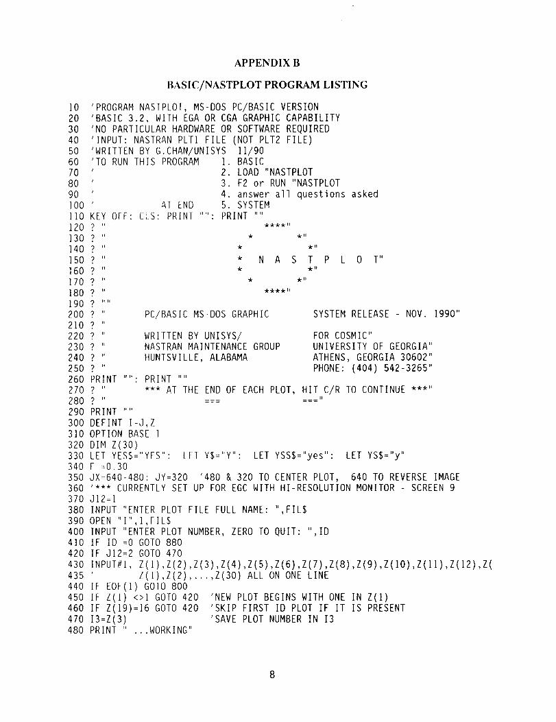
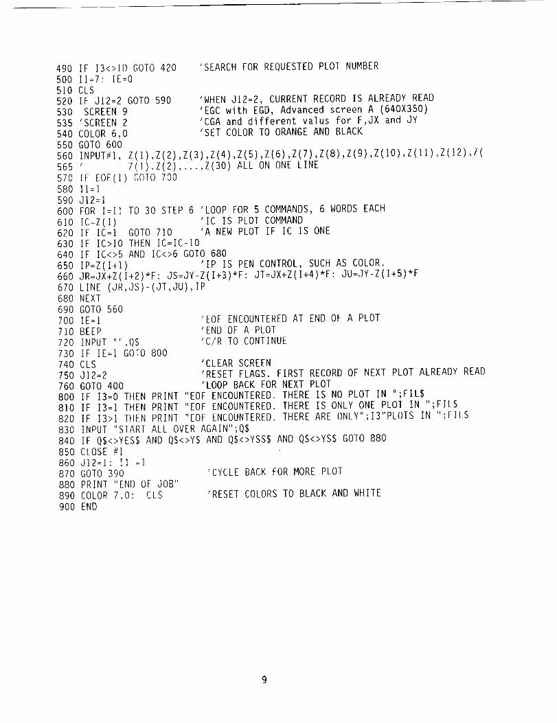
program, with complete listing in Appendix ]3, serves as a demonstration of tapping into thePC world. It can be easily converted to other non MS-DOS systems, such as the Apple andMacintosh.
APPENDIX A
TWO SAMPLES OF NASTRAN PLOT COMMANDS
Sample Plot Commands from a PLT2 file:
(3_0 _teslrecord)
_@_@_@_@_@-@_A_@.@-@-F_@-@_@`@_@_@.@_@_@-@_@_@_.@_@_@.@-@-@.@_@.@_@[email protected]_@.@_@-@_@.@.@_@_@_@_@`@.@.@.@_@_@_@_@.@_@_@.@-@.@.@
`_.C_`g_0_g_0_._*_C.@_._`_`g_`_@_@_._._@_._._.g_@._._._g`_`g.@_g_@_.@._@_`@._._.@._*_
Sample Plot Commands from a PLT1 file:
(130 cot umns/record)
I 0
6 1
6 1
6 1
6 1
6 1
6 1
6 1
1 1023 1023 0 2 2
0 1009 1019 1009 6 I
0 994 1019 994 6 I
0 979 1019 979 6 I
0 964 1019 964 6 1
0 604 1019 604 6 I
0 589 1019 589 6 I
0 574 1019 574 6 I
0 0 0 0 3 2 0 0 0 0 16 I 0 1015 1019 1015 6 I 0 1012 1019 1012
0 1006 1019 1006 6 I 0 1003 1019 1003 6 I 0 1000 1019 1000 6 I 0 997 1019 997
0 991 1019 991 6 I 0 988 1019 988 6 I 0 985 1019 985 6 I 0 982 1019 982
0 976 1019 976 6 I 0 973 1019 973 6 I 0 970 1019 970 6 I 0 967 1019 967
0 961 1019 961 6 I 0 958 1019 958 6 I 0 955 1019 955 6 I 0 952 1019 952
0 601 1019 601 6 I
0 586 1019 586 6 I
0 571 1019 571 6 I
0 598 1019 598 6 I 0 595 1019 595 6 I 0 592 1019 592
0 583 1019 583 6 I 0 580 1019 580 6 I 0 577 1019 577
0 568 1019 568 15 I 197 555 199 555 5 I 199 555 198 555
5 I 198 555 198 550 5 I 198 550 197 549 5 I 197 549 195 549 5 I 195 549 194 550 5 I 202 555 202 550
5 I 202 550 203 569 5 I 203 549 206 549 5 I 206 549 207 550 5 I 207 550 207 555 5 I 215 554 214 555
5 I 216 555 211 555 5 I 211 555 210 556 5 I 210 556 210 553 5 I 210 553 211 552 5 I 211 552 216 552
5 I 287 538 286 539 5 I 286 539 283 539 5 I 283 539 282 538 5 I 282 538 282 534 5 I 282 534 283 533
5 1 283 533 286 533 5 I 286 533 287 534 5 I 287 534 287 536 5 I 287 536 285 536 16 1 0 0 1019 0
6 1 0 3 1019 3 6 1 0 6 1019 6 6 1 0 9 1019 9 6 I 0 12 1019 12 6 I 0 15 1019 15
6 I 0 18 1019 18 6 I 0 21 1019 21 6 1 0 24 1019 24 6 I 0 27 1019 27 6 I 0 30 1019 30
6 1 0 33 1019 33 6 1 0 36 1019 36 6 1 0 39 1019 39 6 1 0 42 1019 42 6 1 0 45 1019 45
5 I 121 1012 122 1011 5 I 122 1011 126 1011 5 I 126"1011 127 1012 5 I 127 1012 127 1016 5 1 1017 1016 1018 1017
5 I I01B 1017 1018 1011 5 1 1018 1011 1017 1011 5 1 1017 1011 1019 1011 0 0 0 0 0 0 0 0 0 0 0 0
15 I 9 59 12 59 5 I 12 59 12 53 5 I 12 53 12 59' 5 I 12 59 15 59 5 I 22 59 17 5
5 I 17 59 17 56 5 I 17 56 20 56 5 I 20 56 17 56 5 I 17 56 17 53 5 I 17 53 22 53
APPENDIX B
BASIC/NASTPLOT PROGRAM LISTING
I0 'PROGRAM NASTPLOT, MS-DOS PC/BASIC VERSION20 'BASIC 3.2, WITH EGA OR CGA GRAPHIC CAPABILITY30 'NO PARTICULAR HARDWARE OR SOFTWARE REQUIRED40 'INPUT: NASTRAN PLTI FILE (NOT PLT2 FILE)50 'WRITTEN BY G.CHAN/UNISYS 11/9060 'TO RUN THIS PROGRAM 1. BASIC70 ' 2. LOAD "NASTPLOT80 ' 3. F2 or RUN "NASTPLOT90 ' 4. answer all questions asked
-k'l
* N A S T P
9¢ _,i
I00 ' AT END 5. SYSTEM110 KEY OFF: CI.S: PRINT .... : PRINT ....
PC/BASIC MS-DOS GRAPHIC
WRITTEN BY UNISYS/NASTRAN MAINTENANCE GROUPHUNTSVILLE, ALABAMA
260 PRINT .... : PRINT ""
120130140 9150 9160 9170180190 9200 9210220 9230 9240 9250 9
L 0 T"
SYSTEM RELEASE - NOV. ]990"
FOR COSMIC"UNIVERSITY OF GEORGIA"ATHENS, GEORGIA 30602"PHONE: (404) 542-3265"
270 9 "280 _ " ---"290 PRINT ....300 DEFINT I-J,Z310 OPTION BASE ]320 DIM Z(30)330 LET YES$="YES": LET Y$="Y": LET YSS$="yes":340 F =0.30
*** AT THE END OF EACH PLOT, HIT C/R TO CONTINUE ***"
LET YS$="y"
350 JX=640-480:JY=320 '480 & 320 TO CENTER PLOT, 640 TO REVERSE IMAGE360 '*** CURRENTLY SET UP FOR EGC WITH HI-RESOLUTION MONITOR - SCREEN 9370 J12=I380 INPUT "ENTER PLOT FILE FULL NAME: ",FIL$390 OPEN "I",],FIL$400 INPUT "ENTER PLOT NUMBER, ZERO TO QUIT: ",ID4]0 IF ID =0 GOTO 880420 IF 012=2 GOTO 470430 INPUT#l, Z(I),Z(2),Z(3),Z(4),Z(S),Z(6),Z(l),Z(e),z(9),Z(lO),Z(II),Z(12),Z(435 ' Z(]),Z(2) ..... Z(30) ALL ON ONE LINE440 IF EOF(1) GOTO 800450 IF Z(1) <>l GOTO 420 'NEW PLOT BEGINS WITH ONE IN Z(I)460 IF Z(19)=16 GOTO 420 'SKIP FIRST ID PLOT IF IT IS PRESENT470 13=Z(3) 'SAVE PLOT NUMBER IN 13480 PRINT " ...WORKING"
490 IF 13<>IDGOTO420500 I]=7: IE=O510 CLS520 IF J12=2 GOTO590530 SCREEN9535 'SCREEN2540 COLOR6,0550 GOTO600
SEARCHFORREQUESTEDPLOTNUMBER
WHENJ12=2, CURRENTRECORDIS ALREADYREADEGCwith EGD,Advancedscreen A (640X350)
'CGAand different valus for F,JX and JY'SET COLORTOORANGEANDBLACK
560 INPUT#1,Z(1),Z(2),Z(3),Z(4),Z(5),Z(6),Z(7),Z(8),Z(9),Z(IO),Z(II),Z(12),Z(565 ' Z(I)>Z(2) .... ,Z(30) ALL ON ONE LINE570 IF EOF(I) GOTO 700580 11=]590 J]2=]600 FOR I=11 TO 30 STEP 6 'LOOP FOR 5 COMMANDS, 6 WORDS EACH610 IC=Z(1) 'IC IS PLOT COMMAND620 IF IC=I GOTO 710 'A NEW PLOT IF IC IS ONE630 IF IC>IO THEN IC=IC-IO
640 IF IC<>5 AND IC<>6 GOTO 680
650 IP=Z(I+I) 'IP IS PEN CONTROL, SUCH AS COLOR.
660 JR=JX+Z(I+2)*F: JS=JY-Z(I+3)*F: JT=JX+Z(I+4)*F: JU=JY-Z(I+5)*F
670 LINE (JR,JS)-(JT,JU),IP68O NEXT
690 GOTO 560700 IE=]710 BEEP
720 INPUT .... ,QS730 IF IE=I GOTO 800740 CLS750 J]2=2760 GOTO 400
'EOF ENCOUNTERED AT END OF A PLOT'END OF A PLOT'C/R TO CONTINUE
'CLEAR SCREEN'RESET FLAGS. FIRST RECORD OF NEXT PLOT ALREADY READ'LOOP BACK FOR NEXT PLOT
800 IF 13=0 THEN PRINT "EOF ENCOUNTERED. THERE IS NO PLOT IN ";FIL$8]0 IF 13=1 THEN PRINT "EOF ENCOUNTERED. THERE IS ONLY ONE PLOT IN ";FIL$820 IF 13>] THEN PRINI "EOF ENCOUNTERED. THERE ARE ONLY";13"PLOTS IN ";FIL$830 INPUT "START ALL OVER AGAIN";Q$840 IF Q$<>YES$ AND Q$<>Y$ AND Q$<>YSS$ AND Q$<>YS$ GOTO 88085O CLOSE #1860 J12=I: 11 =I870 GOTO 390880 PRINT "END OF JOB"890 COLOR 7,0: CLS90O END
'CYCLE BACK FOR MORE PLOT
'RESET COLORS TO BLACK AND WHITE
9
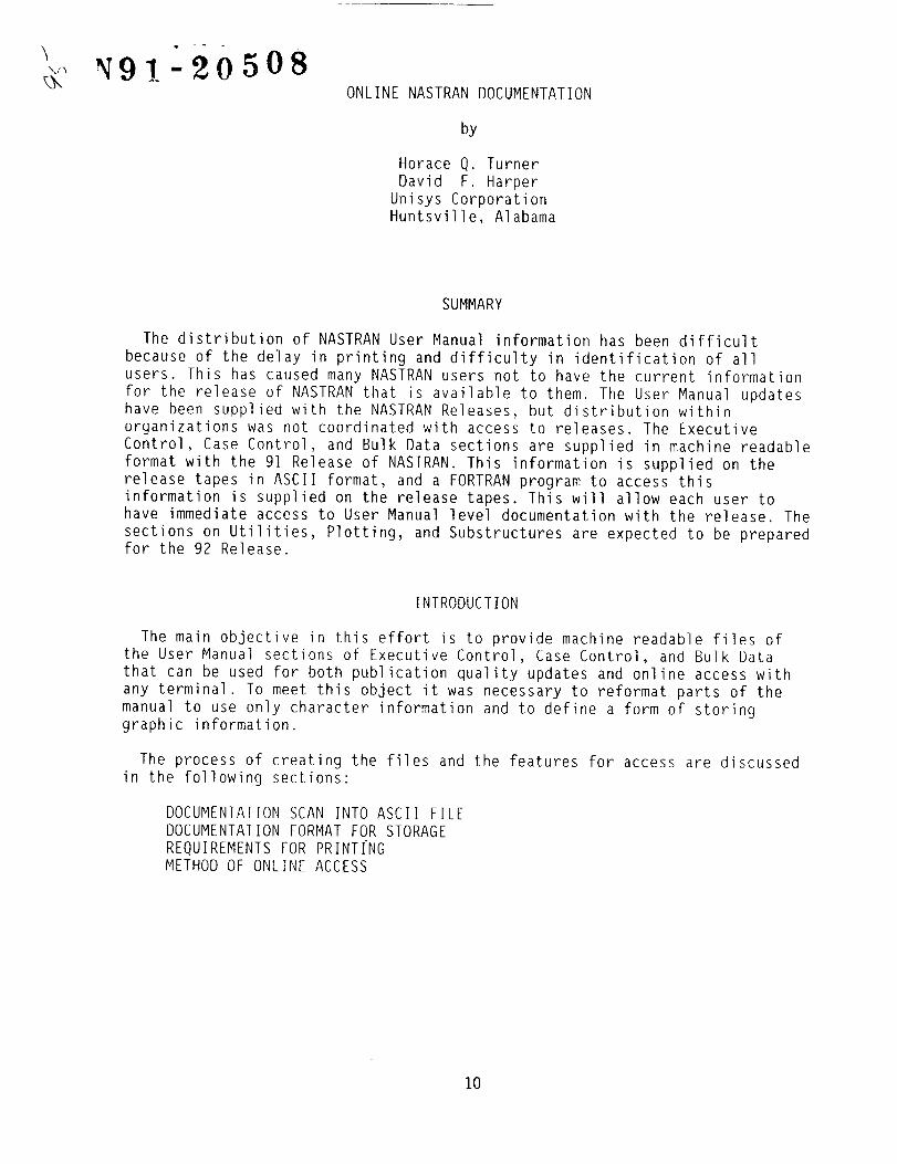
N91-20508ONLINE NASTRAN DOCUMENTATION
by
Horace q. TurnerDavid F. Harper
Unisys CorporationHuntsville, Alabama
SUMMARY
The distribution of NASTRAN User Manual information has been difficultbecause of the delay in printing and difficulty in identification of allusers. This has caused many NASTRAN users not to have the current informationfor the release of NASTRAN that is available to them. The User Manual updateshave been supplied with the NASTRAN Releases, but distribution withinorganizations was not coordinated with access to releases. The ExecutiveControl, Case Control, and Bulk Data sections are supplied in machine readableformat with the 91 Release of NASTRAN. This information is supplied on therelease tapes in ASCII format, and a FORTRAN program to access thisinformation is supplied on the release tapes. This will allow each user tohave immediate access to User Manual level documentation with the release. Thesections on Utilities, Plotting, and Substructures are expected to be preparedfor the 92 Release.
INTRODUCTION
The main objective in this effort is to provide machine readable files ofthe User Manual sections of Executive Control, Case Control, and Bulk Datathat can be used for both publication quality updates and online access withany terminal. To meet this object it was necessary to reformat parts of themanual to use only character information and to define a form of storinggraphic information.
The process of creating the files and the features for access are discussedin the following sections:
DOCUMENTATION SCAN INTO ASCII FILEDOCUMENTATION FORMAT FOR STORAGEREQUIREMENTS FOR PRINTfNGMETHOD OF ONLINE ACCESS
10
DOCUMENTATIONSCANINTOASCII FILE
The first step in preparation of the User Manual sections for online accesswas to scan the existing manual sections into machine readable format. Thiswas done using a scanner integrated with a PCcomputer. The output of the scanwas an ASCII file containing only character data. The figures and line datawere dropped during the scan. The scanner used was a Kurzweil device locatedat a government facility in Huntsville, Alabama. The scanner software was ableto read the reduced pages and different font styles that had been used inpreparation of the User Manual over the years. The scanner software wastrainable for recognition of overstrike characters as required in the UserManual.
DOCUMENTATION FORMAT FOR STORAGE
To meet the objective of maintaining the User Manual sections in onedatabase format for both publishing quality and online access, the followingrules were used for the document storage format:
Stored in page format by card type
All lines reduced to 80 characters
Page length is 82 lines
All graphics removed
All subscripts and superscripts replaced
All equations written in FORTRAN notation
PC box drawing codes are used to represent line data
No embedded codes are used for formatting
No overstrike or underline characters
The document is stored in line per record format with each section of thedocument in a separate file.
The Executive Control and Case Control sections required the most change inappearance of tile pages Attached is a sample page showing the replacement ofthe large "()" by PC box drawing characters. This will allow for substitutionof these characters on any terminal.
The Bulk Data section maintains most of its appearance with the lines andfigures replaced by PC box drawing characters.
11
REQUIREMENTSFORPRINTING
The documentcan be printed on an HP LaserJet or compatible with legal sizepaper using 6 lines per inch and the native 10 character per inch Courier fontcontaining PC box drawing characters. This page then has to reduced to 85percent to produce a standard 8.5 by I] inch manual update page. To print onother devices the PC box drawing characters can be replaced. This replacementcan be done with an editor or a program to translate the file.
METHOD OF ONLINE ACCESS
A FORTRAN program to read and display the pages on the screen is supplied onthe 91 Release tapes. This program allows the user to select the section andthe key topic for display. The key topic is a Bulk Data, Executive Control, orCase Control card name. This program allows the user to set the number oflines for display on the output device and stops when that number of lines isdisplayed. At any time, the user can back up or advance a specified number oflines. This program assumes the terminal can only display standard ASCIIcharacters, and therefore converts the PC box drawing _haracters to +, -, andI for display. The figures that can be stored in this format will be shown onthe display.
12
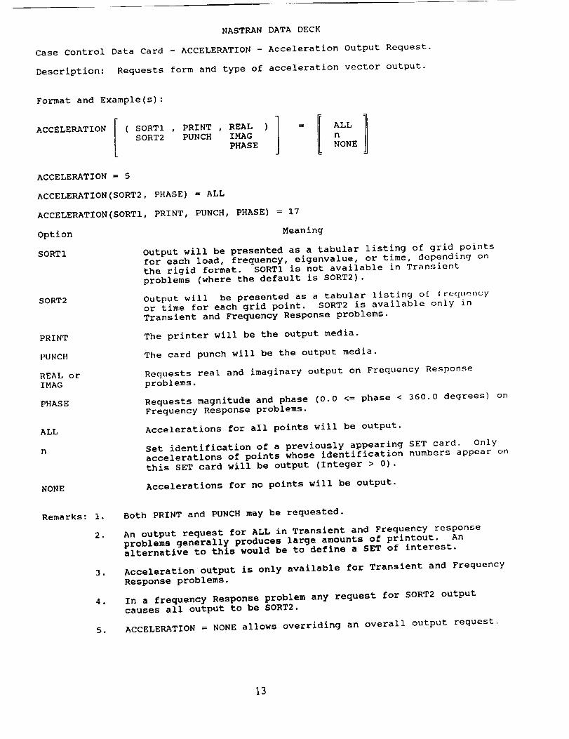
NASTRAN DATA DECK
Case Control Data Card - ACCELERATION - Acceleration Output Request.
Description: Requests form and type of acceleration vector output.
Format and Example(s):
CCL TIO[COiPRINTRALSORT2PCPAIOO1 ALL
n
NONE
ACCELERATION = 5
ACCELERATION(SORT2, PHASE) = ALL
ACCELERATION(SORT1, PRINT, PUNCH, PHASE) = 17
Option Meaning
SORTI Output will be presented as a tabular listing of grid points
for each load, frequency, eigenvalue, or time, depending on
the rigid format. SORT1 is not available in Transientproblems (where the default is SORT2).
SORT2 Output will be presented as a tabular listing o[ [req_lency
or time for each grid point. SORT2 is available only in
Transient and Frequency Response problems.
PRINT The printer will be the output media.
PUNCH The card punch will be the output media.
REAL orIMAG
Requests real and imaginary output on Frequency Response
problems.
PHASE Requests magnitude and phase (0.0 <= phase < 360.0 degrees) on
Frequency Response problems.
ALL Accelerations for all points will be output.
Set identification of a previously appearing SET card. Only
acceleratlons of points whose identification numbers appear on
this SET card will be output (Integer > 0).
NONE Accelerations for no points will be output.
Remarks: i.
2.
3.
4 .
5,
Both PRINT and PUNCH may be requested.
An output request for ALL in Transient and Frequency response
problems generally produces large amounts of printout. Analternative to this would be to define a SET of interest.
Acceleratlon output is only available for Transient and Frequency
Response problems.
In a frequency Response problem any request for SORT2 output
causes all output to be SORT2.
ACCELERATION = NONE allows overriding an overall output request.
13
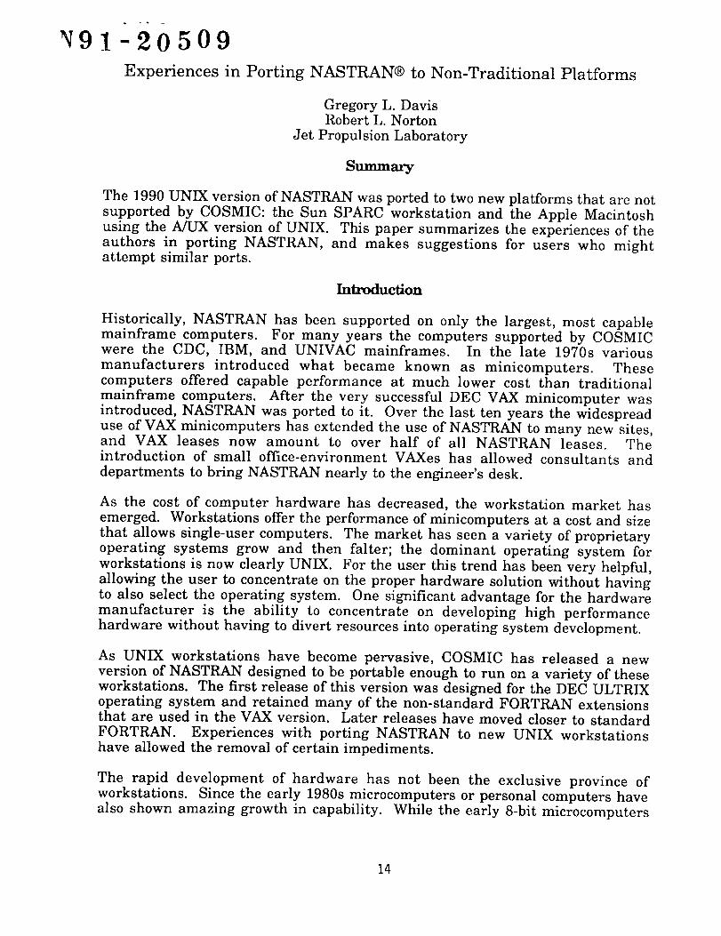
91-20509
Experiences in Porting NASTRAN® to Non-Traditional Platforms
Gregory L. DavisRobert L. Norton
Jet Propulsion Laboratory
Summary
The 1990 UNIX version of NASTRAN was ported to two new platforms that are not
supported by COSMIC: the Sun SPARC workstation and the Apple Macintosh
using the A/UX version of UNIX. This paper summarizes the experiences of the
authors in porting NASTRAN, and makes suggestions for users who mightattempt similar ports.
Introduction
Historically, NASTRAN has been supported on only the largest, most capable
mainframe computers. For many years the computers supported by COSMICwere the CDC, IBM, and UNIVAC mainframes. In the late 1970s various
manufacturers introduced what became known as minicomputers. Thesecomputers offered capable performance at much lower cost than traditional
mainframe computers. After the very successful DEC VAX minicomputer was
introduced, NASTRAN was ported to it. Over the last ten years the widespreaduse of VAX minicomputers has extended the use of NASTRAN to many new sites,and VAX leases now amount to over half of all NASTRAN leases. The
introduction of small office-environment VAXes has allowed consultants and
departments to bring NASTRAN nearly to the engineer's desk.
As the cost of computer hardware has decreased, the workstation market has
emerged. Workstations offer the performance of minicomputers at a cost and size
that allows single-user computers. The market has seen a variety of proprietary
operating systems grow and then falter; the dominant operating system for
workstations is now clearly UNIX. For the user this trend has been very helpful,
allowing the user to concentrate on the proper hardware solution without havingto also select the operating system. One significant advantage for the hardware
manufacturer is the ability to concentrate on developing high performance
hardware without having to divert resources into operating system development.
As UNIX workstations have become pervasive, COSMIC has released a new
version of NASTRAN designed to be portable enough to run on a variety of theseworkstations. The first release of this version was designed for the DEC ULTRIX
operating system and retained many of the non-standard FORTRAN extensions
that are used in the VAX version. Later releases have moved closer to standardFORTRAN. Experiences with porting NASTRAN to new UNIX workstations
have allowed the removal of certain impediments.
The rapid development of hardware has not been the exclusive province of
workstations. Since the early 1980s microcomputers or personal computers have
also shown amazing growth in capability. While the early 8-bit microcomputers
14
were almost useless for finite element analysis, some work could be done on the 16-bit microcomputers of the middle to late 1980s. With the introduction of highspeed 32-bit microcomputers, the boundary between workstations andmicrocomputers has become blurred. The cost of workstations has droppedenough that low-end workstations are cheaper than high-end personalcomputers, while the performance of high-end personal computers approachesthe performance of workstations.
Many people have wrestled with the definitions of workstations and personalcomputers. Rather than focus on hardware to establish the difference, it makesmore sense to look at the differences from the user's point of view. One big appealof the personal computer has always been the vast array of software available.Few engineers would want to do without the personal productivity software theynow routinely use. The vast volume of personal computers along with therelatively small number of display devices allows the development of nichesoftware to go with the high volume software (e.g. word processors,spreadsheets). Probably the strongest feature of workstations is the robustness ofUNIX. While it is trivial to write a program to crash a personal computer, it ismuch more difficult to crash UNIX.
Naturally enough, most engineers don't want to choose only the personalproductivity software of the personal computers or only the robustness of UNIX --they want both on their desktop at the same time. Thus hardware manufacturersare producing computers that run both UNIX and traditional personal computeroperating systems. There are many computers using Intel architecture that runUNIX and MS-DOS programs. Apple has available A/UX (their version of UNIX),which also runs regular Macintosh software and can even run MS-DOS softwarein emulation mode. The workstation hardware manufacturers are counteringwith Reduced Instruction Set Computers (RISC) that also run MS-DOS inemulation. One manufacturer has even announced a laptop RISC machine thatruns UNIX, MS-DOS, and Macintosh software.
One clear winner has emerged from the confusion of operating systems andcomputer architecture -- the end user. We now have available an amazing,almost paralyzing set of options. For the NASTRAN community this revolutionmeans that "NASTRAN for the masses" is at hand. We have $10,000 desktop
computers that are at least as capable as the multi-million-dollar mainframes
that were used at the dawn of NASTRAN twenty years ago. Manufacturers have
recently announced portable UNIX computers that are fully capable of runningNASTRAN. Now the individual engineer can not only have NASTRAN at the
desk, but also can carry NASTRAN to the work!
General Porting Comments
The sheer size of NASTRAN is one of the biggest obstacles to porting. The 1990
VAX version has 84 machine-dependent subroutines (0.3 MBytes) and 1695
machine-independent subroutines (13.3 MBytes), for a total of 1779 subroutines
(13.7 MBytes). This size has always created problems for NASTRAN, and it
15
typically pushes the boundaries of the computer and operating systemcapabilities.
Although the VAX version has been all FORTRAN, a number of VAX extensionsto FORTRAN have been used. UNISYS has been trying to eliminate as manyextensions as possible, but a number of extensions to FORTRAN are still used.Following is a summary of the extensions used, along with some suggestions forporting:
. Some non-standard variable types are used: REAL*4, REAL*8, INTEGER*2,
INTEGER*4, and LOGICAL*I. These extensions are often supported, but if not
they can be easily changed.
. Hexadecimal constants are used, and the required form of the hexadecimalconstants may vary from one compiler to another. The hexadecimal edit
descriptor z and the octal edit descriptor o are used in the FORMAT statement.
3. Some non-standard functions are used: IAND, IOR, IEOR, ISHFT, JMOD, and
NOT. All of these except JMOD are used in bit manipulation.
4. In-line comments are used, with ! signifying the beginning of the comment.
5. Hollerith constants are used in DATA statements.
6. The alternate RETURN specifier is used with & to indicate the statement label.Change the & to * to meet the standard.
7. READONLY is used in a file OPEN statement in subroutine DSXOPN.
. File names in READ and WRITE statements are stored in arrays (usingHollerith constants) rather than using CHARACTER variables. Thesereferences should be changed to use CHARACTER variables.
9. Variable names exceed the 6 characters permitted by the standard.
10. DISP= rather than STATUS= is used in several CLOSE statements.
11. TYPE= rather than STATUS= is used in an OPEN statement.
12. The %LOC function is used to return the location in memory where a variableis stored.
13. Lower case source code is used.
14. Subroutines CPUTIM, TDATE, and WALTIM are used to get the cpu time, date,
and all clock time from the system. The calls from these subroutines to getthe system level information will be different for each new port.
16
Most of the extensions can be worked around• The truly significant extensionsare the use of the %LOC and the non-standard functions• All of the above
extensions are located in the machine-dependent subroutines, identified by the•MDS extension on the VAX. All the machine-independent routines, identified by
the . MIS extension, compiled on the Sun and the Macintosh with no changes atall.
Sun Porting Experiences
The 1990 UNIX release of NASTRAN was shipped to JPL from UNISYS on a TK50
tape, where it was read onto a VAX ULTRIX machine and copied over to a Sun
4/390 using FTP. The ensuing porting and debugging process fell into three main
stages•
Stage 1 consisted of fixing initial, fairly obvious incompatibilities between the Sun
and VAX FORTRAN compilers. The machine-dependent subroutines were
initially screened for the incompatibilities listed above in General Porting
Comments. After all subroutines were compiled, the 15 executable NASTRAN
links were generated• Gordon Chan of UNISYS was frequently consulted at this
stage of the process and he provided invaluable assistance•
Stage 2 consisted of modifying the ancillary UNIX shell scripts used to drive the
executable NASTRAN links. The script problems originally became apparent in
trying to run sample problem D01000A. NID, when the proper UNIX links could
not be established. XQT and @XQT are well-written UNIX shell scripts to provide a
friendly user interface for running the NASTRAN program; however, these had
to be modified to properly represent the user directory structure and to properly
establish the UNIX links between the rigid format and the alter files•
Stage 3 consisted of debugging the executable links. Problems in execution
became immediately apparent when trying to run sample problem D011A. miD.
The first problem was eventually traced to bit shifting operations in subroutine
KHRFNI: see point 2 under Recommendations to Users for details• A second
problem in execution was traced to subroutine INTPK in link 4. This was
inadvertently repaired by relinking link 4 with INTPK included twice in the link
statement. Link ordering does become crucial! This ad hoc fix was then applied
to all NASTRAN links containing INTPK. These repairs finally permitted the
successful execution of test problem D01011A. miD on the Sun computer.
Macintosh Porting Experiences
The first major challenge with the Macintosh version was getting the source code
downloaded to the Macintosh from the VAX. The only connection was via a 9600-
baud local area network. Kermit was used to automatically download all thesubroutines, which took about 10 hours• The UNIX versions of the machine-
dependent subroutines were obtained via FTP from the Sun computer.
17
The FORTRAN compiler supplied with A/UX does not have the extensionsrequired to properly compile the machine-dependent subroutines, so a third-partyFORTRAN compiler sold by NKR Research, Inc. of San Jose, California wasselected. NKR proved to be very helpful during this project, providing usefuladvice and compiler updates on a timely basis.
The organization of the files on the Macintosh took a couple of tries to get right.A/UX allows the use not only of the usual UNIX editors, vi and ed, but also ofMacintosh graphical user interface editors, such as TextEditor (supplied byApple with A/UX), QUED/M (a commercial editor), or Alpha (a shareware editor).
Unfortunately, since the Macintosh file system does not adequately handle
directories with large numbers of files, the source files cannot be stored together
in one directory. The UNIX file system does cope with large directories, but the
Macintosh editors use the Macintosh file system to open the files. The source fileswere put into 26 directories corresponding to the first letter of the subroutine
name. In this way the largest directory had only 253 files.
The next hurdle was using the UNIX ar utility to create the library of object files.
The VAX and other UNIX systems put all the object files together in one library.This library is then used as input to the linker to form each of the 15 executable
files. The ar utility supplied with A/UX could not load all the object files into the
library. After about 1400 files, it produced an error message when additional files
were to be added to the library. In addition to the error in creating the library, it
took one hour to load the object files into the library. To avoid the library problem
all the object files were copied to a single directory. Since no Macintosh programs
would be used in this directory, the weakness of the Macintosh file system did notmatter. To link the executable files, a list of all the subroutines used in a link was
generated on the VAX and used as input to the A/UX linker.
Recommendations to UNISYS
As the current maintenance contractor to COSMIC, UNISYS has done a splendid
job in producing the UNIX version of NASTRAN. UNISYS has spent severalyears reducing the number of non-standard extensions to FORTRAN used in the
code and has ported NASTRAN to several UNIX platforms.
There is a fundamental tension between the desire to produce a truly generic
version which can be ported to new UNIX platforms relatively easily and the
desire to optimize the code for a particular platform. The various proprietary
versions of NASTRAN will probably continue to be more efficient than the generic
version on any given platform, and some users will always complain. However, it
is in the best interests of COSMIC and UNISYS to place the emphasis on
portability. As the hardware manufacturers continue their rapid performance
improvements, it seems to make more sense to upgrade the hardware than to
"tweak" the code for improved performance.
From our experience in these ports of NASTRAN, we have several suggestions forUNISYS:
18
• NASTRAN is, of course, a rather old code, and FORTRAN has seen manychanges since the FORTRAN IV that was used in the beginning. FORTRAN 77introduced features that could simplify the code and also help the reading andmaintainability of the code. The FORTRAN 90 that is currently being reviewedwill introduce even more radical changes. UNISYS should move toward theuse of structured programing. While it is possible to carry this to extremeswith overly deeply nested IF clauses, a gradual transition to the use of the IF -
THEN - END IF rather than repeated co TO statements would help readability.
After FORTRAN 90 becomes approved and supported, constructs such as DO
WHILE and DO - END DO would also be helpful. The 1990 NASTRAN release
does not use IF - THEN - END IF anywhere.
• The bit handling features of the code should be modernized by using charactervariables. Character variables were not available in the FORTRAN compilers
used when these routines were written and the available computer memory
was meager, so non-standard bit handling techniques were used. Now that
NASTRAN is routinely used on computers with several hundred to several
thousand times as much memory as the 16k-word IBM 7094 and since the
FORTRAN 77 compilers support character variables, it is time to eliminate the
bit manipulation.
• Have a dedicated UNIX machine at UNISYS connected to the Internet, thereby
greatly facilitating program development and user/vendor communications.
Program fixes and enhancements could then be transmitted using FTP, anduser/vendor messages could be transmitted through e-mail.
• Provide the UNIX NASTRAN source codes and related shell scripts on media
other than the TK50 tape, which is VAX specific. Other common media on
UNIX-based "mainframe" type machines are 1/4 inch tape cartridges and 8 mm
cassette tapes. CD-ROMs would provide a wonderful distribution media,
especially when the manuals become available in electronic form.
Recommendations to Users
Porting NASTRAN to other computer platforms is an ambitious undertaking. At
the outset the authors counsel patience and perseverance -- the very large
amount of code will probably stretch the computer's and user's resources to the
limit. The following general approach for porting the UNIX version of NASTRANover to other platforms profits from our own experience and mistakes.
. Copy the NASTRAN source code over to the host machine, renaming the files
as appropriate for the host's FORTRAN compiler. We highly recommend
maintaining the MDS /MI S distinction in the directory structure -- most of the
coding incompatibilities will be in the . MDS routines. It is also a good idea to
make a write-protected copy of all subroutines in the .MDS directory to
preserve the capability to recover from inadvertent or incorrect edits during
the debugging process. Develop a bookkeeping system to keep track of the
large number of subroutines.
19
.
,
.
.
.
.
Initially screen the .MDS subroutines for coding incompatibilities with thehost FORTRAN compiler. Prime candidates for compiler-dependent
problems are listed in the above General Porting Comments. Comment any
changes made for future reference.
Bit shifting operations using the subroutine khrfnl need to be examined.
This may or may not be a problem depending upon the convention for ordering
the position in a character variable. Specifically, the character position of theVAX word is numbered left to right; the corresponding Sun and Macintosh
word is numbered right to left. The current code assumes the VAX
convention. This problem may arise in the .gIs subroutines XSEM01-15,which are the main drivers for each executable link.
Compile the source code. If the compiler has an option to produce a symboltable for a debugger, enabling it will prove very handy later. The .gIS
subroutines should compile uneventfully; the . MDS subroutines may still have
additional bugs. Debug any new errors and comment any changes for future
reference. Successful compilation is no guarantee of successful linking or
successful execution.
Upon completion of (3), archive the object modules using the supplied shell
scripts to form the main library. If building the library exhausts the usable
memory, subdivide the libraries into smaller, more manageable units or place
all the object modules in one subdirectory and do without a library.
Upon completion of (4), build the 15 executable links using the suppliedmakefiles. Libraries containing certain intrinsic functions, or those
supporting the VMS extensions, may have to be explicitly included in the link
statement. Any unresolved cross-references among the subroutines will
appear as errors here. Debug any new errors and comment the changes for
future reference. Successful compilation and linking are no guarantee of
successful execution.
Upon completion of (5), begin running the sample problems using thesupplied shell scripts. Sample problems D 01000A. N I D and D 01001 A. N ID are
tests of LINK1, a good, simple initial test. At this stage, bugs will be more
difficult to run down. The system debugging utility could prove invaluablehere; however, there is one caveat: NASTRAN is so large that it may overload
the symbol tables used by the debugger, giving incorrect error diagnoses. You
then must resort to using strategically placed WRITE statements to debug.
After an error in a particular link is located, the following is a convenient way
to test the fix. Initially, it is not necessary to rebuild the library; instead, the
subroutine containing the prospective fix can be inserted directly into the link
statement. Generate the appropriate makefile for the link being debugged
based on the makelinkl model supplied. Insert the debugged subroutine after
$ (BLKDAT) and before $ (LIB). Linking is order dependent. Regenerate the
new executable link from this makefile. The fix can be tested by either
rerunning the NASTRAN program from the beginning (LINK1) or having
2O
saved the FORTRAN I/O files at the successful termination of the previous
link, rerunning only the repaired link. If all is well, the library can then be
rebuilt and all the links regenerated from the updated library.
Iterate through steps (6) and (7) until all of the sample problems run properly.
Implications for COSMIC
As it becomes easier to port NASTRAN to a wide variety of platforms, COSMIC is
forced to deal with several difficult issues. The first of these issues is the question
of how many versions of NASTRAN COSMIC should officially support. The
present four versions could be drastically multiplied if COSMIC were to provide
an official version for each of the hardware manufacturers that desires a port.
One proprietary version of NASTRAN supports 15 different manufacturers, and
some manufacturers require more than one version. This would be an intolerable
burden for COSMIC and UNISYS. COSMIC's position is that only the current
four versions will be supported, leaving the users, hardware manufacturers, and
third-party software companies responsible for porting NASTRAN to other
platforms.
This leads to the second issue. Once these new ports of NASTRAN have been
accomplished, how does COSMIC control their quality? No one wants to see a
situation where any number of people can make available new ports of NASTRAN
and sell them without having some provision for quality control. The suggestion
of the NASTRAN Advisory Group has been for COSMIC and UNISYS to work on
an expanded suite of demonstration and validation problems. Only after a
company certified that their port successfully passes this expanded suite would
the company be allowed to advertise their port of NASTRAN. This is probably the
best solution for now, but the policy might have to adjust over time.
The development of powerful desktop computers, both workstations and personal
computers, combined with the UNIX version of NASTRAN has turned the dream
of desktop NASTRAN into a reality. Enterprising users can do the port
themselves, and third-party software companies will undoubtedly provide
NASTRAN on a wide variety of computers. This development is a tribute to the
original designers of NASTRAN, who provided such a robust program structure.
This could well be the beginning of a new era of NASTRAN use, with the potentialto provide an even better product, arising from the synergies of interaction
between COSMIC and the new, expanded user community.
Acknowledgment
This paper presents research results carried out in part at the Jet Propulsion
Laboratory, California Institute of Technology, under contract with the National
Aeronautics and Space Administration (NASA).
21
' 91-2051b
MODELING OF CONNECTIONS BETWEEN SUBSTRUCTURES
Thomas G. Butler
BUTLER ANALYSES
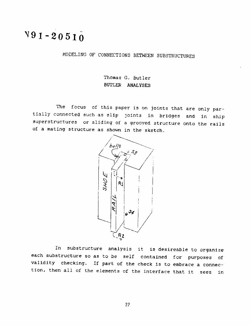
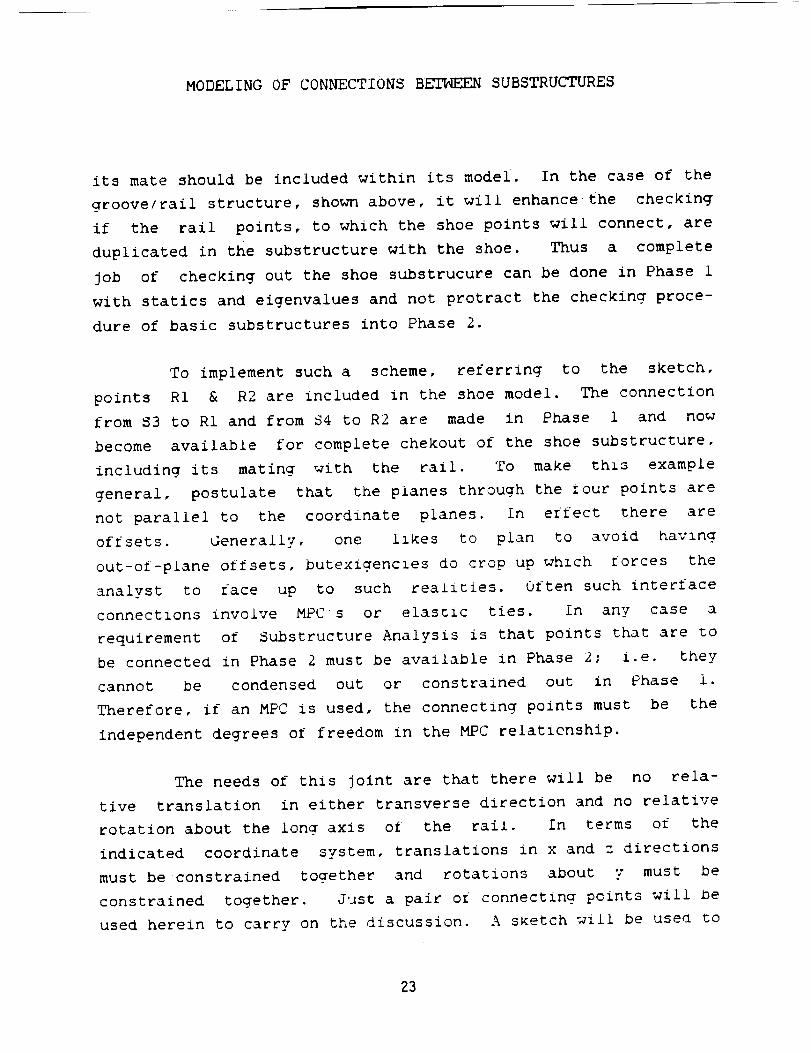
The focus of this paper is on joints that are only par-
tially connected such as slip joints in bridges and in ship
superstructures or sliding of a grooved structure onto the rails
of a mating structure as shown in the sketch.
14,1 -.
In substructure analysis it is desireable to organize
each substructure so as to be self contained for purposes of
validity checking. If part of the check is to embrace a connec-
tion, then all of the elements of the interface that it sees in
2?
MODELINGOF CONNECTIONSBETWEENSUBSTRUCTURES
its mate should be included within its model. In the case of the
groove/rail structure, shown above, it will enhancethe checking
if the rail points, to which the shoe points will connect, areduplicated in the substructure with the shoe. Thus a complete
job of checking out the shoe substrucure can be done in Phase 1
with statics and eiqenvalues and not protract the checkinq proce-
dure of basic substructures into Phase 2.
To implement such a scheme, referring to the sketch,
points R1 & R2 are included in the shoe model. The connection
from $3 to R1 and from $4 to R2 are made in Phase 1 and now
become available for complete chekout of the shoe substructure,
including its mating with the rail. To make thls example
general, postulate that the planes through the :our points are
not parallel to the coordinate planes, in effect there are
offsets. Generally, one likes to plan to avoid havina
out-ol-plane offsets, butexi_encies do crop up which forces the
analyst to face up to such realities. Often such interface
connectlons involve MPC s or elastic ties. in any case a
requirement of Substructure Analysis is that points that are to
be connected in Phase 2 must be available in Phase 2; i.e. they
cannot be condensed out or constrained out in Phase 1.
Therefore, if an MPC is used, the connecting points must be the
independent degrees of freedom in the MPC relatlenship.
The needs of this joint are that there will be no rela-
tive translation in either transverse direction and no relative
rotation about the long axis of the rail. In terms of the
indicated coordinate system, translations in x and z directions
must be constrained together and rotations about v must be
constrained together. Just a pair of connecting points will De
used herein to carry on the discussion. A sketch will be use_ _o
23
MODELINGOF CONNECTIONSBETWEENSUBSTRUCTURES
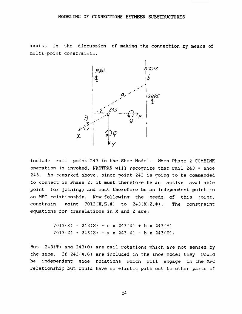
assist in the discussion
multi-point constraints.
RAIL
X
If
4
J 1-c Z4I
Y
of making the connection by means of
l
f
1701Z
I
Include rail point 243 in the Shoe Model. When Phase 2 COMBINE
operation is invoked, NASTRAN will recognize that rail 243 = shoe
243. As remarked above, since point 243 is going to be commanded
to connect in Phase 2, it must therefore be an active available
point for joining; and must therefore be an independent point in
an MPC relationship. Now following the needs of this joint,
constrain point 7013(X,Z,#) to 243(X,Z,#). The constraint
equations for translations in X and Z are:
7013(X) = 243(X) - c x 243(#) + b x 243(_)
7013(Z) = 243(Z) + a x 243(#) - b x 243(@).
But 243(_) and 243(@) are rail rotations which are not sensed by
the shoe. If 243(4,6) are included in the shoe model they would
be independent shoe rotations which will engage in the MPC
relationship but would have no elastic path out to other parts of
24
MODELINGOF CONNECTIONSBETWE2/_SUBSTRUCTURES
the shoe. Thus, if nominal mass were added to these rail points
to keep the eiqenvalue matrix from being singular, an eiqenvalue
check for rigid body modes would show the shoe model to fail.
One might argue, why not leave the rotations in until they are
connected during COMBINE, then they are no longer disjoint. I
cannot afford to leave the 243(4,6; rotations in the shoe model,
because after connecting with the rail these rail rotations must
no____ttbe transmitted back to the shoe. Moments in the shoe/rail
configuration about the two transverse axes are produced only by
couples of forces not by local rotational bending. This rules
out the use of MPC's during Phase 1 in this case. There are
other cases of connections between substructures in which MPCJs
in Phase I would work. The case in which there were no
transverse offsets would work. A NASTRAN run or a simple model
demonstrates these results in Appendix A.
The alternative is to make a stlff elastic connection,
but not so stiff as to cause matrix lll-conditioninq. If a bar
instead of elastic scalars is used, it will be modeled so as to
be fully connected in all 6 degrees of freedom at the shoe end,
but only partially connected at the rail end. At the rail end it
must allow for sliding along the rail and not transmit rotations
to the shoe about the rail transverse axes. This implies that
pin flags must be used at the rail and to inhibi_ these freedoms.
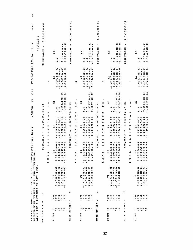
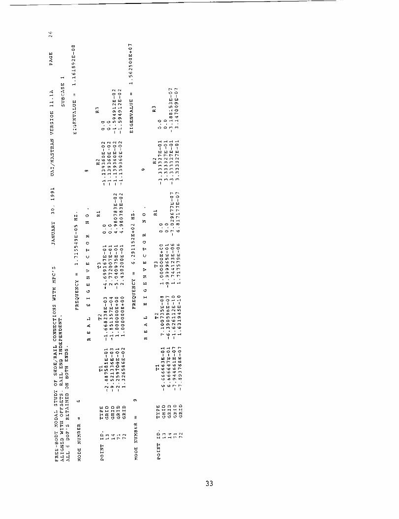
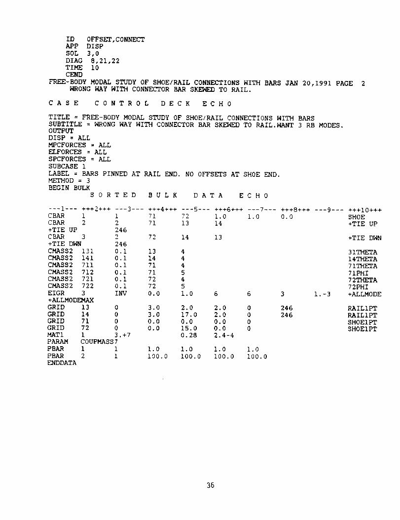
This stiff bar connection can be implemented the wron_
way or the right way. One gets trapped into modelina the wrong
way by forgetting that pin flags are applied to Dar coordinates
not to the displacement coordinates. I fell into this trap and
will show you what happens. Then I will follow it up with the
correct way to model it.
25
MODELING OF CONNECTIONS BETWEEN SUBSTRUCTURES
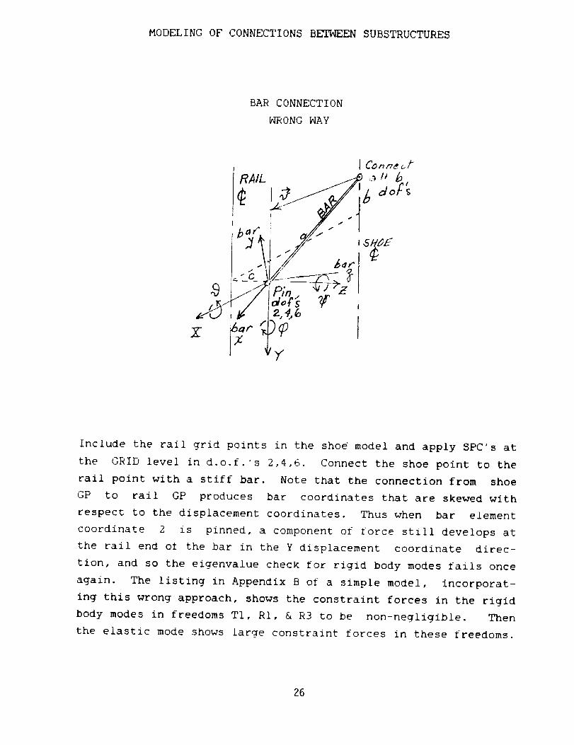
BAR CONNECTION
WRONG WAY
RAIL
,4,6
Y
b
Include the rail grid points in the shoe model and apply SPC's at
the GRID level in d.o.f._s 2,4,6. Connect the shoe point to the
rail point with a stiff bar. Note that the connection from shoe
GP to rail GP produces bar coordinates that are skewed with
respect to the displacement coordinates. Thus when bar element
coordinate 2 is pinned, a component of force still develops at
the rail end ot the bar in the Y displacement coordinate direc-
tion, and so the eigenvalue checM for rigid body modes fails once
again. The listing in Appendix B of a simple model, incorporat-
ing this wrong approach, shows the constraint forces in the rigid
body modes in freedoms TI, RI, & R3 to be non-negligible. Then
the elastic mode shows tarqe constraint forces in these freedoms.
26
MODELING OF CONNECTIONS BETWEEN SUBSTRUCTURES
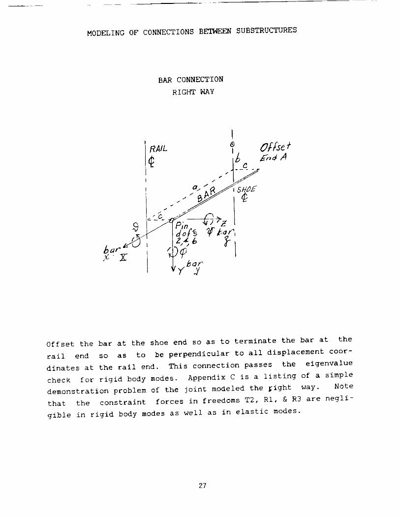
BAR CONNECTION
RIGHT WAY
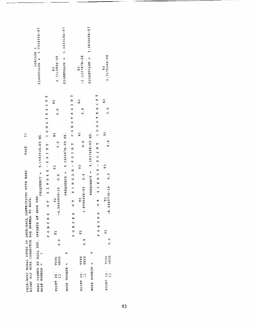
Offset the bar at the shoe end so as to terminate the bar at the
rail end so as to be perpendicular to all displacement coor-
dinates at the rail end. This connection passes the eiqenvalue
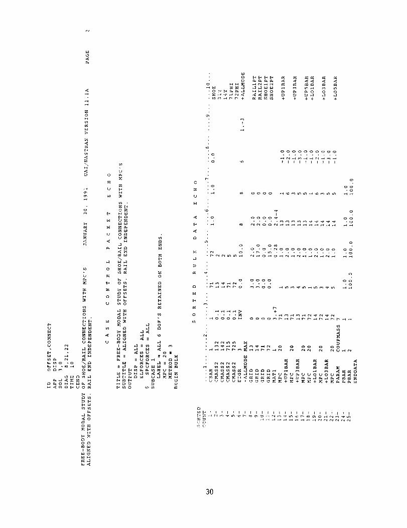
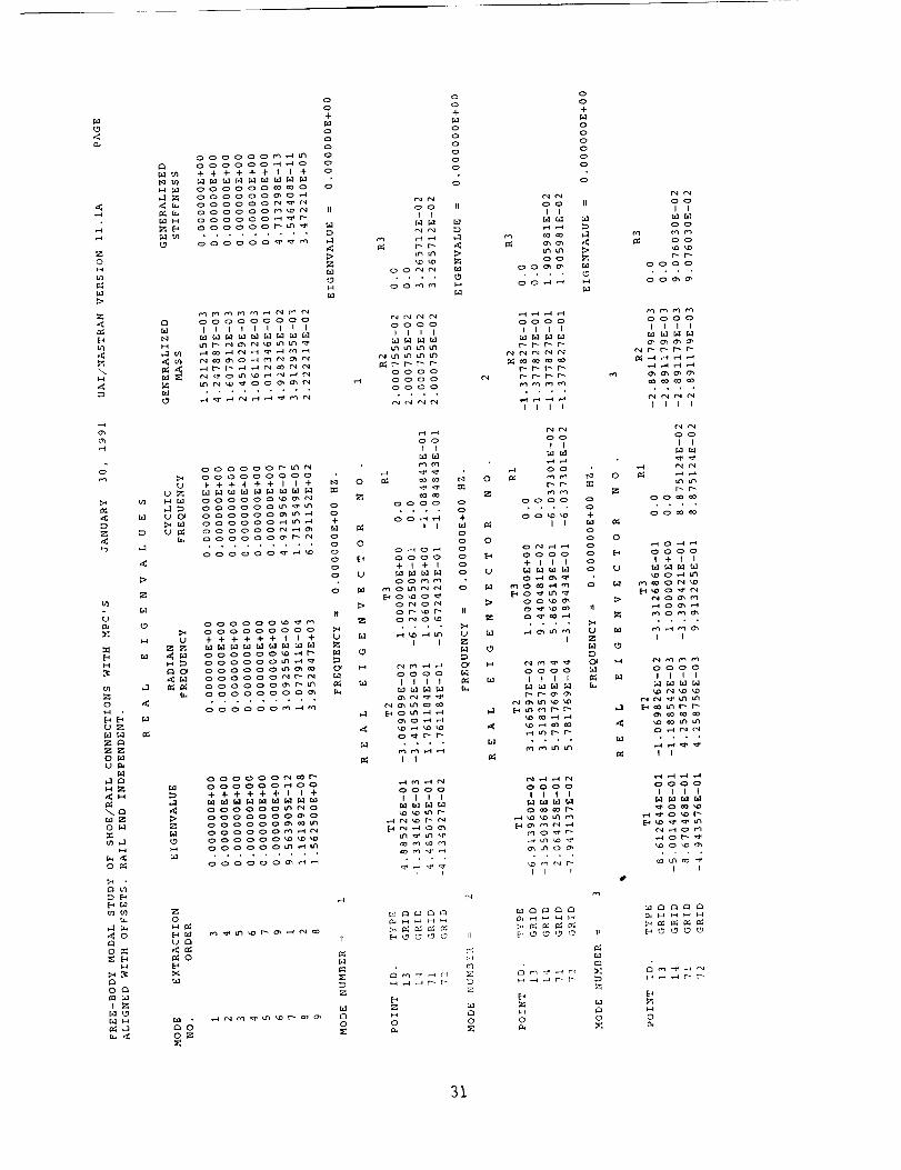
check for rigid body modes. Appendix C is a listing of a simple
demonstration problem of the joint modeled the Fight way. Note
that the constraint forces in freedoms T2, RI, & R3 are negli-
gible in riqid body modes as well as in elastic modes.
27
MODELINGOF CONNECTIONSBETWEENSUBSTRUCTURES
CONCLUSIONS
This paper has demonstrated that complete checkout of a
basic substructure can be done under the special circumstances of
a sliding connection with offsets. Stiff bar connections make
this possible so long as the bar coordinates are aligned with the
displacement coordinates at the sliding surface.
28

MODELING OF CONNECTIONS BETWEEN SUBSTRUCTURES
APPENDIX A
RUN WITH MPC CONNECTION
Z9
L_<
<,-¢
,-4
ZO
H
_>
Z\
O_
Or_
b
O
ZZ
O_0 U_
O_m O_
_Mmm
<0
O_
_M
M_
MH
U0
U
u O_
_ 0OH
0 _
0
am _0 D_
O__ o
O_ _II
_U on_11 _ i1_
IIUO_ _
_ _110_II_ _OU_ _
0 HHE _ _ _ _ _
• 0_ _00 _ _ _0 0 0'__ _ D D D_ _
._+ _ + + ++ + +
?,-¢
, o ..........
o _ , , , ,??????
r--
0
U
'4D
,'_ • 0
<
r',cn
o
o o• o
Toooo_ oo
oo o o co
, o .o ,c_o o o ooooo o o o o, o
D
_ o
I 0 0000 O0
__ ..... i 0
..... _ _ ° a_ ° _8
• _ 0 _ _ _ _
Oo
3O
,<
Z
0H
k]
0"1
Z
o_
oh
oe,q
Z,<to
UO.i
,'M
Z
0H .
_ r_U Z
Z_
0U
I4
_Z
_Z0 c_
0 _
N •
0 121en W
o
o+
o
oo
ooo_oo_ oooo oo_o o_ ++++++11+ o
_ oooooo_o o
_ oooooo_
,<>Z
L9H
M
OO
+
O
OOO
OO
O
OO _I
OOOOOOOOO _
_ ......... oooo
o
o+
oo
oo
o
oo IIII
mm
mm _
oo_ M
ooII
oo
oo
oooo
oooo ooooIIII 1111
,,,, 7777
0000 0000 .U ++++++II+ N 0
U_ oooooo_ o_ OOOOOO_ +
oooooo_ o
oooooo_ o
o
oo oo oo
11 11 II
_ . _ oo . _ __ _ 0 _m _ 0 _
II _ _ Jl _
o _o 0 0
+I+I 0 +III 0 I+II
00_ • 0_ _0_
_0_0_> o_o_
0o0000_ _ ....o oooo oooo _ ....
H U ++++++11+ U _ _ _
_ 000000_ _ 0000_ oooooo_ _ _ IIII _ m
_Z _oo++++++11+
_ _o_O_o _000000_
o_oo_o_o oo om_m
_o_
o_
Z0
_O
m
DZ
_O O
o_ 11 _o_
J / !
OOOO _ OOO0I111 _ _ IIII
r-4
u]_D
Z
0 0
$,
• m d
Z
0 0 0
31
o
o+
oo
o_q
ul o
• -I ,J_ r,1
0
<
cq
,'-4
0
' 01".1
'_ 0
00 t.)0
00+
ooo
o
o
oo tlII
mm _
oo_ H
_m_m
IIII
IIII
_m
II
_ _ 0
_ o
o+ I
oo o
oooo
oo II oo IIII II
II _ II
ooII
oo_
0000 0000 0000IIII IIII IIII
IIII I I
oo oo ooII II II
_ . _ oo • _ _0 _ _ 0 __ _ O0 _ _
oo_ o oo_ _ oo_.... o .... o ....
_ II _ _ II
IIII o tlll _ II+I
0
ca I_
0
b_r_ .
H rn
0_0
_ tq H
0 _ II
r_ 0 rn
0_
I _
_<< 0
II Z _ Z _ Z
.... _ ....
I I
O0I+II _ _ IIII
_ _ooo ....
T _ _TT _
_ o
o o o oooo o o+ l + I I + I + I I I I + I I I
o u% o r-_ ko o _o o ,--# co u_ ,-_ o co o'_ o_
,_,f......, , , 7_? .....
0 0 0 0 0 0 0
32
a0
o
L9 r.1
_-, O_cO
,-t U_ ::,
0 _>
H Z
H
Z<
Z
\
o_0_
o
Z
o
÷
o
o
oo II
II
oo_
II
oo
11
_o
0000 0000IITF tIT;
,,, 7_7 _
oo ooII II
0 _ _ _ 0 _ _
00_ _ 000_
.... 0 ....00_ + 00_
_ _ _ I
0 _ 0
IIII _ +111
_o_
II _ IIZ _0_
L
,.r,
oH •
0
_ •
o_._
_0H _]D
0
<0_
_ II
ra 0 _
0_ :_
l_ ,-1 ,--1 0
_o_o_
o_o_
IPlP
OOOO OOOOllll
I It
_MHMH _HNHH
Z
z N z0 0 0
33

MODELING OF CONNECTIONS BETWEEN SUBSTRUCTURES
APPENDIX B
RUN WITH WRONG BAR CONNECTION
34
GRIDP0 INTID. TYPE
71 G
72 G
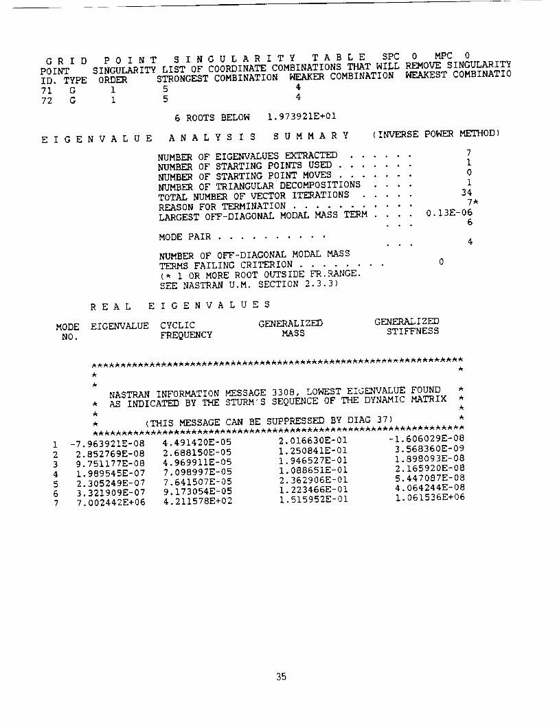
P 0 I N T S I N G U L A R I T Y T A B L E SPC 0 MPC 0
SINGULARITY LIST OF COORDINATE COMBINATIONS THAT WILL REMOVE SINGULARITYORDER STRONGEST COMBINATION _[EAKER COMBINATION _AKEST COMBINATI0
1 5 4
1 5 4
6 ROOTS BELOW 1.973921E+01
E I G E N V A L U E A N A L Y S I S S U M M A R Y (INVERSE POWER METHOD)
NUMBER OF EIGENVALUES EXTRACTED ...... 7NUMBER OF STARTING POINTS USED ....... 1
NUMBER OF STARTING POINT MOVES ....... 0
NUMBER OF TRIANGULAR DECOMP0SITIONS .... 1
TOTAL NUMBER OF VECTOR ITERATIONS ..... 34REASON FOR TERMINATION ........... 7*
LARGEST 0FF-DIAGONAL MODAL MASS TERM .... 0.13E-06
6
MODE PAIR ..........
NUMBER OF 0FF-DIAGONAL MODAL MASS
TERMS FAILING CRITERION ........
(* 1 OR MORE ROOT OUTSIDE FR.RANGE.SEE NASTRAN U.M. SECTION 2.3.3)
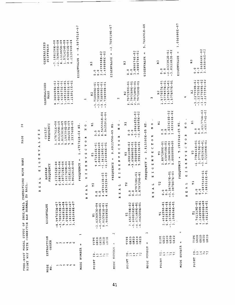
REAL E I GENVALUES
MODE EIGENVALUE CYCLIC GENERALIZED GENERALIZED
NO. FREQUENCY MASS STIFFNESS
NASTRAN INFORMATION MESSAGE 3308, LOWEST EIGENVALUE FOUND *AS INDICATED BY THE STURM'S SEQUENCE OF THE DYNAMIC MATRIX *
• (THIS MESSAGE CAN BE SUPPRESSED BY DIAG 37) *
1 -7.963921E-08 4.491420E-05
2 2.852769E-08 2.688150E-05
3 9.751177E-08 4.969911E-05
4 1.989545E-07 7.098997E-05
5 2.305249E-07 7.641507E-056 3.321909E-07 9.173054E-057 7.002442E+06 4.211578E+02
2.016630E-01
1.250841E-01
1.946527E-01
1.088651E-01
2.362906E-011.223466E-01
1.515952E-01
-1.606029E-08
3.568360E-09
1.898093E-08
2.165920E-08
5.447087E-084.064244E-081.061536E+06
35
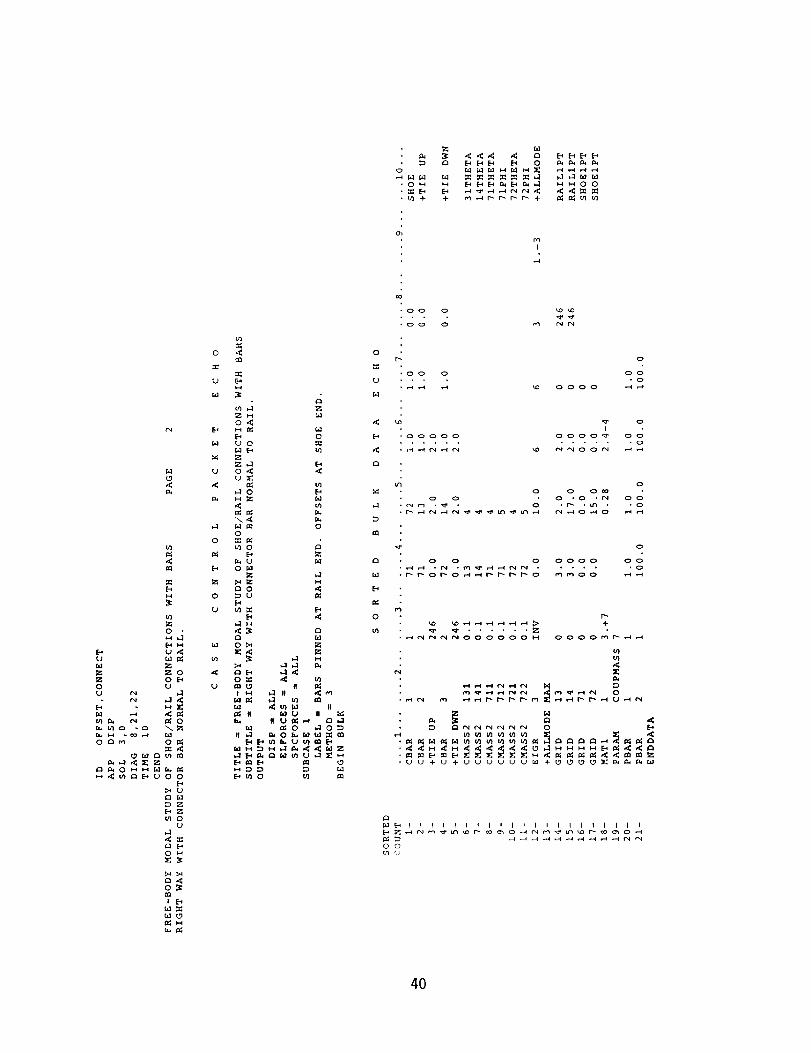
ID 0FFSET,CONNECTAPP DISPSOL 3,0DIAG 8,21,22TIME i0CEND
FREE-BODYMODALSTUDYOF SHOE/RAILCONNECTIONSWITHBARSJAN 20,1991 PAGE_]RONGHAY WITH CONNECTOR BAR SKEWED TO RAIL.
CASE CONTROL DECK ECHO
TITLE = FREE-BODY MODAL STUDY OF SHOE/RAIL CONNECTIONS WITH BARS
SUBTITLE = _TRONG HAY WITH CONNECTOR BAR SKEWED TO RAIL.MANT 3 RB MODES.OUTPUTDISP -- ALL
MPCFORCES = ALL
ELFORCES = ALL
SPCFORCES = ALL
SUBCASE 1
LABEL = BARS PINNED AT RAIL END. NO OFFSETS AT SHOE END.METHOD = 3BEGIN BULK
SORTED BULK DATA ECHO
---I--- +++2+++CBAR 1
CBAR 2
+TIE UPCBAR 3
+TIE DWN
CMASS2 121CMASS2 141
CMASS2 711
CMASS2 712CMASS2 721
CMASS2 722
EIGR 3
1
2
2462
246
0 1
0 10 1
0 10 1
0 1
INV
---3--- +++4+++ ---5--- +++6+++ ---7--- +++8+++ ---9--- +++I0+++
+ALLMODEMAXGRID 13 0
GRID 14 0GRID 71 0
GRID 72 0
MAT1 1 3. +7PARAM COUPMASS 7
PBAR 1 1
PBAR 2 1ENDDATA
71 72 1.0 1.0 0.0 SHOE71 13 14 +TIE UP
72 14 13 +TIE DWN
13 4 31THETA
14 4 14THETA71 4 71THETA
71 5 71PHI
72 4 72THETA72 5 72PHI
0.0 1.0 6 6 3 1.-3 +ALLMODE
3.0 2.0 2.0 0
3.0 17.0 2.0 00.0 0.0 0.0 0
0.0 15.0 0.0 00.28 2.4-4
1.0 1.0 1.0 1.0
i00.0 I00.0 i00.0 i00.0
246 RAILIPT246 RAILIPT
SHOEIPT
SHOEIPT
36
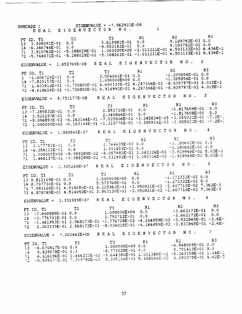
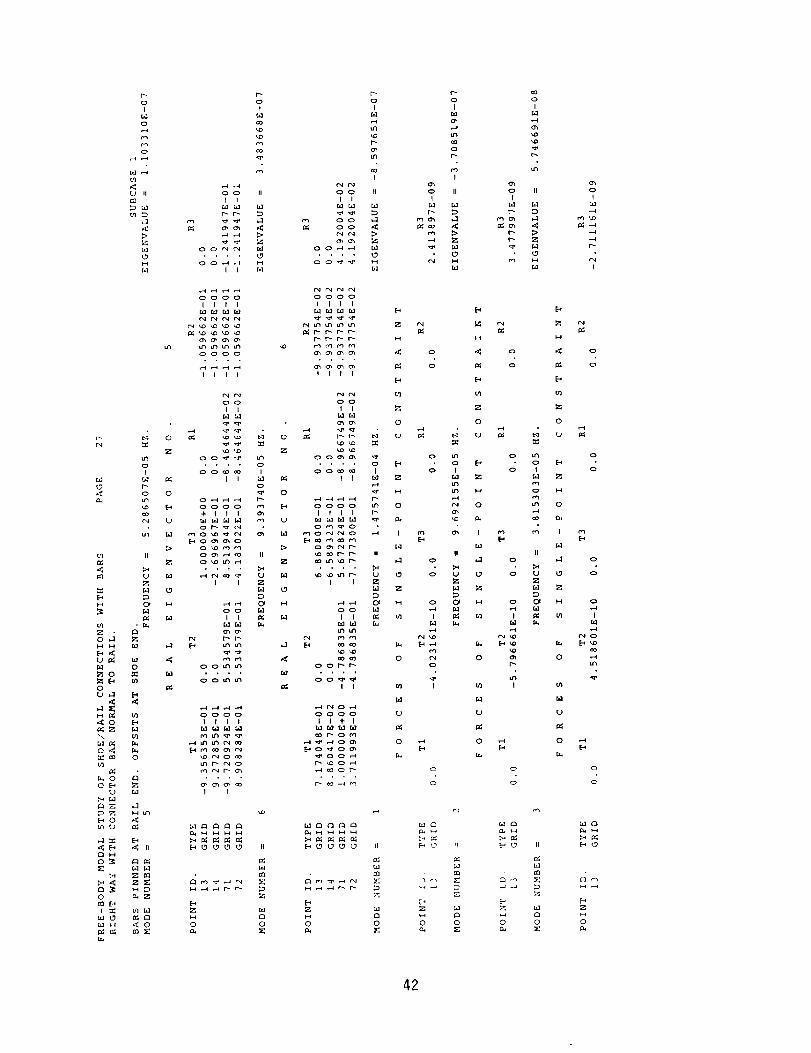
SUBCASE1 EIGENVALUE= -7. 963921E-08REAL E I GENVEC T 0 R NO 1
PT ID. T1 T2 T3 R1 R2 R313 3.308091E-01 0.0 5.615981E-01 0.0 9.189782E-02 0.014 -6.346744E-01 0.0 -9.552183E-01 0.0 9.189782E-02 0.071 3.910763E-01 -5.288029E-01 1.000000E+00 -I.011211E-01 6.503133E-02 6.436E-272 -5.744071E-01 -5.288029E-01 -5.168163E-01 -I.011211E-01 6.503133E-02 6.436E-2
EIGENVALUE= 2.852769E-08 R E A L E I G E N V E C T 0 R N 0 2
PT ID. T1 T2 T3 R1 R2 R31 -1.806720E-01 0.0 3.554041E-01 0.0 -1.205854E-01 0.014 -7.829153E-01 0.0 1.000000E+00 0.0 -1.205854E-01 0.071 1.40381_E-01 -I.730800E-01 4.690333E-02 4.297306E-02 -8.839797E-02 4.015E-272 -4.618614E-01 -1.730800E-01 6.914992E-01 4.297306E-02 -8.839797E-02 4.015E-2
EIGENVALUE= 9.751177E-08 R E A L E I G E N V E C T 0 R N 0 3
PT ID. T1 T2 T3 R1 R2 R313 -7.289532E-01 0.0 2.853720E-01 0.0 -1.817658E-01 0.014 3.520157E-01 0.0 2.345846E-01 0.0 -1.817658E-01 0.071 -8.096893E-02 -6.163144E-01 -7.029006E-02 -3.385834E-03 -2.055022E-01 -7.2E-f72 1.000000E+00 -6.163144E-01 -1.210776E-01 -3.385834E-03 -2.055022E-01 -7.2E-_
EIGENVALUE= 1.989545E-07 R E A L E I G E N V E C T 0 R N 0 4
ID. T1 T2 T3 R1 R2 R313 3.177751E-01 O.0 1.764639E-02 0.0 -3._80602E-01 0.0
14 -4.354112E-01 0.0 3.301453E-01 0.0 -3.1a0602E-01 0.0
71 i.000000E+00 -9.989289E-02 -9.057981E-01 2.083326E-02 -2.929949E-01 5.02E-2
72 2.468137E-01 -9.989289E-02 -5.932992E-01 2.083326E-02 -_.929949E-01 5.02E-2
EIGENVALUE = 2.305249E-07 R E A L E I G E N V E C T 0 R N 0
PT ID. T1 T2 T3 R1 R2 R3
13 9.812109E-01 0.0 1.000000E+00 0.0 -1.272332E-02 0.0
14 8.707730E-01 0.0 5.573768E-01 0.0 -1.272332E-02 0.0
71 7.983168E-01 4.514050E-01 8.229362E-01 -2.950821E-02 -2.407710E-02 7.363E-3
72 6.878789E-01 4.514050E-01 3.803130E-01 -2.950821E-02 -2.407710E-02 7.363E-3
EIGENVALUE = 3.321909E-07 R E A L E I G E N V E C T 0 R N 0 6
PT ID. T1 T2 T3 R1 R2 R3
13 -7.600989E-01 0.0 1.000000E+00 0.0 -3.662173E-01 0.0
14 -3.776701E-01 0.0 3.752712E-01 0.0 -3.662173E-01 0.071 -1.461953E-01 2.568173E-01 -1.776728E-01 -4.164859E-02 -3.932845E-01 -2.6E-
72 2.362335E-01 2.568173E-01 -8.024015E-01 -4.164859E-02 -3.932845E-01 -2.6E-
EIGENVALUE = 7.002442E+06 R E A L E I G E N V E C T 0 R N 0
PT ID. T1 T2 T3 R1 R2 R3
13 -6.670417E-01 0.0 1.000000E+00 0.0 -6.548009E-01 0.014 5.839078E-01 0.0 -8.773038E-01 0.0 5.701413E-01 0.0
71 6.416196E-01 1.446323E-03 -9.644380E-01 2.011386E-'JI -5.263158E-01 1.14E-I72 -5.595077E-01 7.309750E-03 8.305104E-01 5.448166E-0_ 6.091975E-01 4._2E-2
37
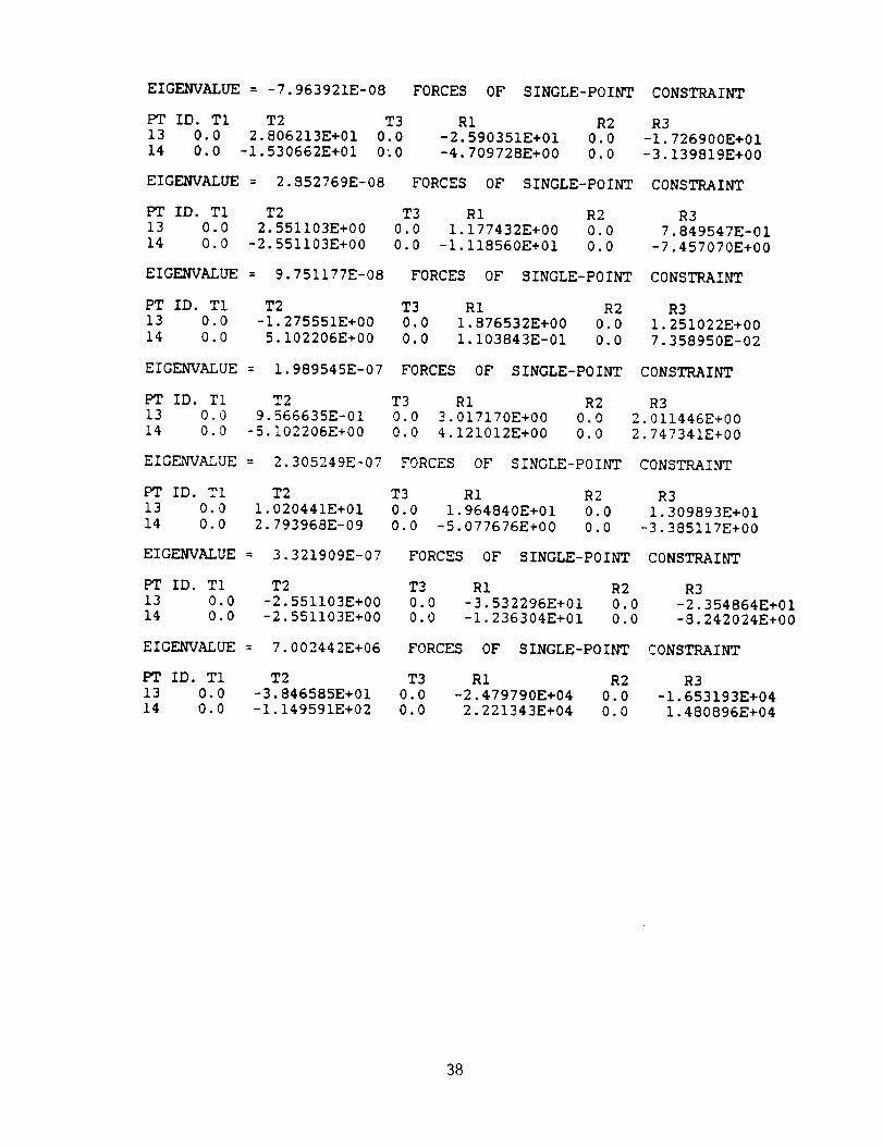
EIGENVALUE : -7.963921E-08 FORCES OF SINGLE-POINT CONSTRAINT
PT ID. T1 T2 T313 0.0 2.806213E+01 0.0
14 0.0 -1.530662E+01 0%0
R1 R2-2.590351E+01 0.0-4.709728E+00 0.0
EIGENVALUE = 2.$52769E-08 FORCES OF SINGLE-POINT
PT ID. T1 T2
13 0.0 2.551103E+00
14 0.0 -2.551103E+00
EIGENVALUE = 9.751177E-08
T3 R1 R2
0.0 1.177432E+00 0.0
0.0 -i.118560E+01 0.0
R3
-1.726900E+01-3.139819E+00
CONSTRAINT
R37.849547E-01
-7.457070E+00
FORCES OF SINGLE-POINT CONSTRAINT
PT ID. T1 T2 T3
13 0.0 -1.275551E+00 0.0
14 0.0 5.102206E+00 0.0
R1 R21.876532E+00 0.0
I.I03843E-01 0.0
R3
1.251022E+00
7.358950E-02
FORCES OF SINGLE-POINT CONSTRAINT
T3 R1 R20.0 3.017170E+00 0.0
0.0 4.121012E+00 0.0
EIGENVALUE = 1.989545E-07
PT ID. T1 T2
13 0.0 9.566635E-0114 0.0 -5.102206E+00
FORCES OF SINGLE-POINTEIGENVALUE = 2.305249E-07
PT ID. T1 T2 T3
13 0.0 1.020441E+01 0.0
14 0.0 2.793968E-09 0.0
R1 R2
1.964840E+01 0.0
-5.077676E+00 0.0
R3
2.011446E+00
2.747341E+00
EIGENVALUE = 3.321909E-07
CONSTRAINT
R3
1.309893E+01-3.385117E+00
FORCES OF SINGLE-POINT CONSTRAINT
R1 R2
-3.532296E+01 0.0-1.236304E+01 0.0
PT ID. T1 T2 T313 0.0 -2.551103E+00 0.0
14 0.0 -2.551103E+00 0.0
FORCES OF SINGLE-POINTEIGENVALUE = 7.002442E+06
R1 R2
-2.479790E+04 0.0
2.221343E+04 0.0
PT ID. T1 T2 T3
13 0.0 -3.846585E+01 0.0
14 0.0 -I.149591E+02 0.0
R3-2.354864E+01
-S.242024E+00
CONSTRAINT
R3
-1.653193E+04
1.480896E+04
38

MODELING OF CONNECTIONS B_ SUBSTRUCTURES
APPENDIX C
RUN WITH RIGHT BAR CONNECTION
39
' _ Q _ _ 0 _
• OH H __ _HO0• _ _ __ _ _ _
0 •H_
U_
_0O_
0 OU _
_ _ _0
0_ O_
__UO0
_U
_0U
O_
O_m
_H
0_n
,I-U
_J_H
O_
E__._ u 0
u 0,_u_
,-I0n. H
:.-I _.I ,_
00 _ I_
,.n 0
r.s.,U0 r.,-1
in 00 _ U
_H
0"U m
0,v.o_
r.1
r..r..
0
M
III H _1 II _m
_ _./) _1 II
6_t_O _ en
_0
-oo o kO_D.... _ "0"
• 00 0 r,q r-¢ r_l
0 'I_ 0
,00 0 00
U ..... 0• ,-I ,-_ ,-4 _lO 0000 ,,-¢ ,--_
b.1
/
• 00000 0000_ O0............ 0
00 0 O_
• 0.0._ O0• 0 0
0
• 0 0 0 0000 O00
0
• _ Q__ 0
'_____
O©
4O
oc-4
,<
I=
0 •H
U<
_0
0_U
H_
M
0 0
Q
U,I
a0 H
Hr,
O
I
II
H
000000
IIIIII
OI
I
II
oo_ H
ooooIIII
tt I
o oI I
oo If O0 I( O0II II II
oo _ _ _ _ _ _
oo_ _ oooo _ oooo
oooo oooo ooooIIII IIII IIII
IIII
000000 .u llllll _ 0
...... _ 0
_nr_
ooII
gg££ _m
m 0
I+II
oo oo ooII II II
_ _ 0 _ _ 0 _
_ 0 _ 0
oooo _ _ _ _ _ ooo o
ll÷l _ m IIII
II
000000H U I l ; I I I U r._
000 O0llllll
r_
II
ooII _
_o ....._oo_ _o _o_
I _ _ I I
O0 _ O0 _ O0II _ _ II _ _ II
.... _ .... _ .°.°oo_ oom_ oo_
oooo 0000 O0 0 0
llll IIII fill II÷I
0
U_ II
E
_0 0
_ tl
0 0
M _m
0 0 0 0 0
41
oI
o
t_
o
H
r--
UlO
n.
O OI I
7oo II oo tt
11 II
oo_ _ oo_.... _ ....
ooooIIII
oooo
TTTT
oI
o_
u_co
or*'-
I
o II
I
r_
_>
0c_l i-i
_0o
I
o_
u'3
o III
r'-- p,Z
0r_ H
O_
0I
r_
I
ooooIIII
II II
. _ _ . _ _ • .0 _ _ 0 _ _
o .... o .... o
_ oooo _ _ oo o o _ 0
ul
..r.
Z •
0 ,,-1H ,',1
tJ ,--1 N
_ m
O._ u.
r_u.o d
_:_ E-_ _ II
P4H _:0p_ _
b_
II
0
(_ H
r,1 O0 _ O0II _ _ II _
00_ 00_.... _ ,o.,
...... TT
o oo oo oIIII II+I
H
0
Z
0
.-e
• 0 ['_0 I
t_ Z
H
t_ 0
IIo _.I
• ;_o _ L9
o O' H
I _
eq
O
Cd
_3
O
E_b_
H
O ,_ O
E-'
Z
O
5:
O u_ O. O E_ *
O I OZ
on
o Hu_ O
co
II0 _ o
o ',3 _ o
r.1 _.
0 01 H o
I _ _ I
0 _ 0
0 _ 0
_0000 II _0000 II
g _
Z Z
N _ NH _
0 0 0 0
c_
O O
n_
n_
O O O
42
o o oI I I
U II 0 II 0 II
H _ H _ H
oIr.1
a3
.-e
O • I_H,-1 Z
Hu4
OZ O "_
O'_ u)K.;
_0 _
mO ,_
.1
0 H
O_ _
I
_ _0
H H H
• . °
o _ o _ o
u} u}
O O O
t_ o ul o i._ o
I o I o I o
_, I_ oo H ',m HOh H
O_ O '.C, O _'_ O
E_ _ E'-'
II II II,-1 O ,..1 o ,-1 o
. Iw • I_ "U _ 0 U _ o U _ O
C_ H ? O_ H C_ CW _ O
l_ l_ I I_ _ I l_ _ I
_l _
0 '_
_d
U
0 _
r,.
o
0 _ 0 _
m I m
U ',J
o _ o
o o
M H HO O O O O
43
91-20511
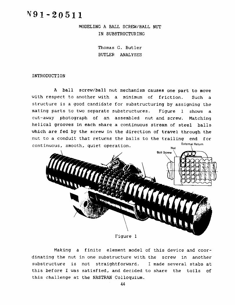
MODELING A BALL SCREW/BALL NUT
IN SUBSTRUCTURING
Thomas G. Butler
BUTLER ANALYSES
INTRODUCTION
A ball screw/ball nut mechanism causes one part to move
with respect to another with a minimum of friction. Such a
structure is a good candidate for substructuring by assigning the
mating parts to two separate substructures. Figure 1 shows a
cut-away photograph of an assembled nut and screw. Matching
helical grooves in each share a continuous stream of steel balls
which are fed by the screw in the direction of travel through the
nut to a conduit that returns the balls to the trailing end for
continuous, smooth, quiet operation.External Return
Nut
Ball S
Figure 1
Making a finite element model of this device and coor-
dinating the nut in one substructure with the screw in another
substructure is not straightforward. I made several stabs at
this before I was satisfied, and decided to share the toils of
this challenge at the NASTRAN Colloquium.
44
BALL SCREH/BALL NUT
PLAN
In the particular application being discussed here, the
screw was attached to the moving structure and the nut was at-
tached to the stationery structure. The object of the overall
analysis was to determine the vibration characteristics of the
whole structure for various configurations; i.e. the evaluation
of the mode shapes and frequencies when parts were moved to
different mating positions. Therefore, it was necessary to
provide for the ball screw to be moved and reconnected to the
ball nut at a number of dlfferenct locations along its length.
The Substructure capability in NASTRAN makes it possible to
prescribe a connection with a COMBINE operation in Phase 2 and
perform an eigenvalue analysis for that configuration. Once
these results are catalogued, the analyst erases these results
and returns to the COMBINE operation for a new set of connections
and performs a second elgenvalue analysis. Succeeding runs can
be made for as many repositionlngs as is desired. The challenge
is in modeling the nut so as to represent both the rigid body
relation of the helix plus the elastic relations of its members.
The scheme then is to model the nut and the screw so as to be
invariant for any combination of positions, such that reposition-
inq is achieved by specifying that location on the screw that is
to be in contact with the nut in the Phase 2 COMBINE step.
MODEL
The first step is to represent the elastic parts in a
simple arrangement. The NUT will consist of two yokes at either
end of the nut and an axial tie between the two yokes. The yoke
models the nut housing that connects the ball interface to the
stationary structure (P). The yoke consists of two bars
extending on either side of the screw (S) centroid to the bolts
in P. The sketch shows this simple arrangement.
45
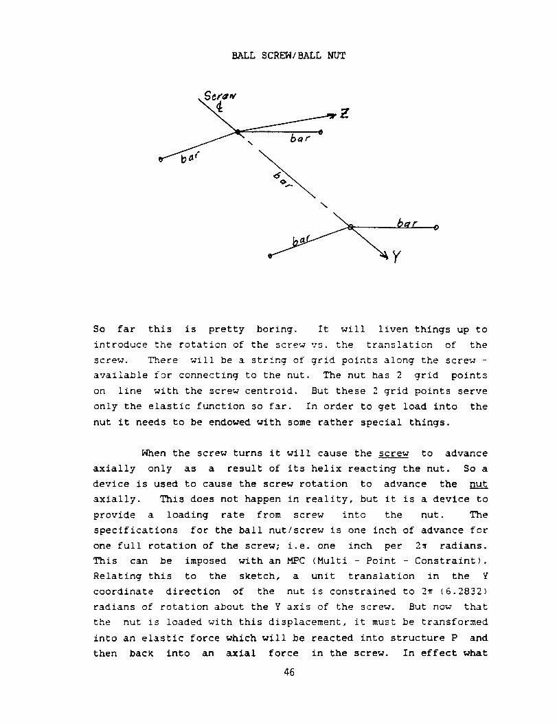
BALL SCREW/BALLNUT
\
o
So far this is pretty boring. It will liven things up tointroduce the rotation of the screw vs. the translation of the
screw. There will be a strinq of grid points along the screw -
available for connecting to the nut. The nut has 2 grid points
on line with the screw centroid. But these 2 grid points serve
only the elastic function so far. In order to get load into the
nut it needs to be endowed with some rather special things.
When the screw turns it will cause the screw to advance
axially only as a result of its helix reacting the nut. So a
device is used to cause the screw rotation to advance the nu___tt
axially. This does not happen in reality, but it is a device to
provide a loading rate from screw into the nut. The
specifications for the ball nut/screw is one inch of advance for
one full rotation of the screw; i.e. one inch per 27 radians.
This can be imposed with an MPC (Multi - Point - Constraint).
Relating this to the sketch, a unit translation in the Y
coordinate direction of the nut is constrained to 2_ (6._8_2)
radians of rotation about the Y axis of the screw. But now that
the nut is loaded with this displacement, it must be transformed
into an elastic force which will be reacted into structure P and
then back into an axial force in the screw. In effect what
46
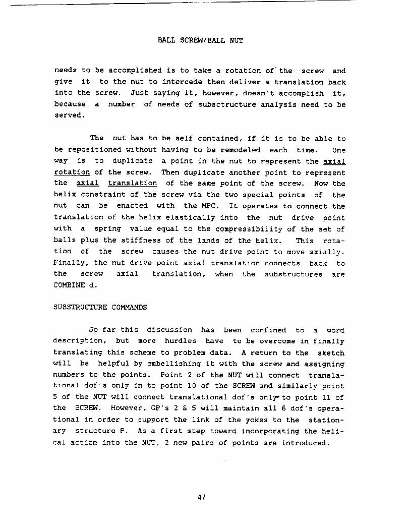
BALL SCREW/BALL NUT
needs to be accomplished is to take a rotation of the screw and
give it to the nut to intercede then deliver a translation back
into the screw. Just saying it, however, doesn't accomplish it,
because a number of needs of subsctructure analysis need to be
served.
The nut has to be self contained, if it is to be able to
be repositioned without having to be remodeled each time. One
way is to duplicate a point in the nut to represent the axial
rotation of the screw. Then duplicate another point to represent
the axial translation of the same point of the screw. Now the
helix constraint of the screw via the two special points of the
nut can be enacted with the MPC. It operates to connect the
translation of the helix elastically into the nut drive point
with a spring value equal to the compressibility of the set of
balls plus the stiffness of the lands of the helix. This rota-
tion of the screw causes the nut drive point to move axially.
Finally, the nut drive point axial translation connects back to
the screw axial translation, when the substructures are
COMBINE'd.
SUBSTRUCTURE COMMANDS
So far this discussion has been confined to a word
description, but more hurdles have to be overcome in finally
translating this scheme to problem data. A return to the sketch
will be helpful by embellishing it with the screw and assigning
numbers to the points. Point 2 of the NUT will connect transla-
tional dof's only in to point I0 of the SCREW and similarly point
5 of the NUT will connect translational dof's only-to point II of
the SCREW. However, GP's 2 & 5 will maintain all 6 dof's opera-
tional in order to support the link of the yokes to the station-
ary structure P. As a first step toward incorporating the heli-
cal action into the NUT, 2 new pairs of points are introduced.
47
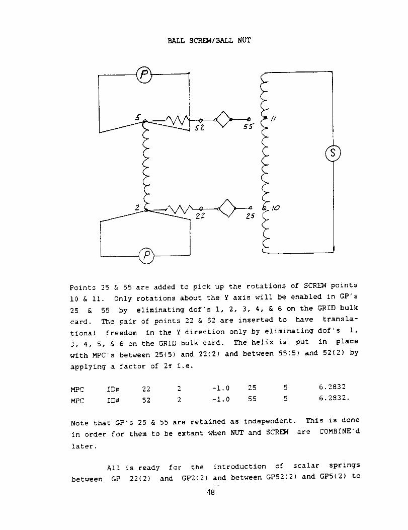
BALL SCREW/BALL NUT
SZ
22
t.
Points 25 & 55 are added to pick up the rotations of SCRk-7_ points
i0 & II. 0nly rotations about the Y axis will be enabled in GP's
25 & 55 by eliminating dof's i, 2, 3, 4, & 6 on the GRID bulk
card. The pair of points 22 & 52 are inserted to have transla-
tional freedom in the Y direction only by eliminating dof's i,
3, 4, 5, & 6 on the GRID bulk card. The helix is put in place
with MPC's between 25(5) and 22(2) and between 55(5) and 52(2) by
applying a factor of 2_ i.e.
MPC ID# 22 2 -I.0 25 5 6.2832
MPC ID# 52 2 -I.0 55 5 6.2832.
Note that GP's 25 & 55 are retained as independent.
in order for them to be extant when NUT and SCREW4
later.
This is done
are C0MBINE'd
between
All is ready for the introduction of scalar springs
GP 22(2) and GP2(2) and between GP52(2) and GP5(2) to
48
_LSCREW/BALLNUT
represent the drive resistance between SCREP{ and NUT which is
carried into the stationary structure by the bars connecting 2 &
5 to GP's i, 2, 4, & 6. The translational response of NUT drive
points 2 and 5 are ready for connecting back to the SCRE_ in a
COMBINE operation.
Now a word about Phase 2 COMBINE operations. If the
automatic option for COMBINE is chosen, it finds all dof's at the
same physical location and ties all like colocated dof's together
unless otherwise inhibited. The substructure control packet will
command that substructure P be COMBINE'd with substructrure S.
In this case the set of GP's 2, i0, 22, & 25 and the set of GP's
5, Ii, 52, & 55 are colocated. It is well to pause to tabulate
what the requirements are and what action is needed to implement
these desires.
I. Requirements
GP 2(1,2,3) should tie to GP 10(1,2,3)
Gp 5(1,2,3) should tie to GP 11(1,2,3).
Remedy
Note is taken that all 6 dof's are active at both points. In
order to limit the tie to only translations, the substructure
bulk data card called RELES is employed to command the release of
dof's 4, 5, & 6 during a COMBINE operation.
2. Requirements
GP 25(5) should tie to GP 10(5).
GF 55(5) should tie to GP 11(5).
Remedy
Since GP's 25 & 55 have only dof 5 active and sin@e the require-
ment is to tie them to dof 5 of GP's 10 & ii respectively, there
is no need to intercede. Allow the automatic option to proceed
unhindered.
. Requirements
GP 22(2) & 52(2) should not tie to any part
substructure S.
of
49
_L SCREW/_L NUT
Remed7
Impose a RELES on GP 22(2) & 52(2)
influence from substructure S.
to keep them free of any
SUMMARY
The action which will ensue from this model is as fol-
lows. NUT point GP 25(5) will pick up the rotation from SCREW
POINT GP 10(5). The MPC will advance the translation of NUT
point GP 22(2) from the rotation of GP 25(5) in the ratio of 1 :
2_. The translation of GP 22(2) will be opposed by the elastic
link to the NUT drive point GP 2(2). This helical loading will
be carried to the NUT housing bars and reacted into the station-
ary substructure P. The net translation in all 3 coordinate
directions of NUT drive point GP 2 will be tied directly into the
3 translationals of SCRE_ substructure drive point i0. A paral-
lel set of actions will also take place between GP's SCREW ii to
55 to 52 to 5 to SCREW Ii. This completes the logic.
As a mathematician would say: "This is a pathological
case", in that such an elaborate device would not have had to be
resorted to for modeling a ball nut, if it were not for the
special requirement of having to reposition the NUT with respect
to the SCREW. The repositioning requirement demanded that the
NUT be self-contained so as to be independent of the relative
locations. Thus, in order to be self-contained, the NUT in
effect picked up the duties of the helical advancement from the
SCREW and carried them out internally in a highly artificial
manner in order to transmit the reaction into the parent struc-
ture before handing back the results of the helical advancement
to the SCREW. As a bonus, this modeling left the analyst free to
reposition the NUT at will along the SCREW4 merely by specifying
the coordinate transformation in moving the SCREW to a new posi-
tion and by specifying new GRID POINT numbers on the RELES cards.
This paper has shown an achievement of a simple set of
operating conditions to an otherwise complicated modeling task.
50
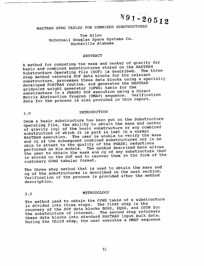
"2051 NASTRAN GPWG TABLES FOR COMBINED SUBSTRUCTURES
Tom Allen
McDonnell Douglas Space Systems Co.Huntsville Alabama
ABSTRACT
A method for computing the mass and center of gravity for
basic and combined substructures stored on the NASTRAN
Substructure Operating File (SOF) is described. The three
step method recovers SOF data blocks for the relevant
substructure, processes these data blocks using a specially
developed FORTRAN routine, and generates the NASTRAN
gridpoint weight generator (GPWG) table for the
substructure in a PHASE2 SOF execution using a Direct
Matrix Abstraction Program (DMAP) sequence. Verification
data for the process is also provided in this report.
1.0 INTRODUCTION
Once a basic substructure has been put on the Substructure
Operating File, the ability to obtain the mass and center
of gravity (cg) of the basic substructure or any combined
substructure of which it is part is lost in a normal
NASTRAN execution. The user is unable to verify the mass
and cg of the subsequent combined substructures nor is he
able to attest to the quality of the PHASE1 reductions
performed on his models. The method described here allows
the user to obtain the mass and cg of any substructure thatis stored on the SOF and to recover them in the form of the
customary GPWG tabular format.
The three step method that is used to obtain the mass and
cg of the substructures is described in the next section.
Verification of the process is provided after the method
description.
2 .0 METHODOLOGY
The method used to obtain the GPWG table of a substructure
is divided into three steps. The first step is the
recovery of the SOF data blocks BGSS, EQSS, and CSTM for
the substructure of interest. The second step reformats
these data blocks into standard NASTRAN input bulk data.
During the third step, the user executes a DMAP sequence
51
that uses the bulk data from the second step to define the
geometry, and the stored mass matrix to calculate the GPWG
table. Each of these three steps will be described below.
2.1 Step 1 - Data Block Recovery
Step 1 of the process involves obtaining the SOF data
blocks BGSS, EQSS, and CSTM for the substructure of
interest from the SOF. The PHASE2 substructure control
deck required for this operation is shown in Figure i. The
data is taken from the SOF and written to NASTRAN file
FORT17. Sample records for each of the three data blocks
are provided in Figure 2.
2.2 Step 2 - Defining Input Bulk Data
Step 2 takes the data blocks recovered from Step 1 andconverts them into standard NASTRAN Bulk Data that is used
to define the geometry of the model. The SOF data blockswill be described below. The bulk data that is created
from the data blocks will also be defined.
2.2.1 BGSS Data Block Description
The BGSS data block contains the location in the basic
coordinate system of each internal point in the
substructure as well as the output coordinate system of the
internal point. If the output coordinate system is -i, the
internal point is a scalar point rather than a physical
gridpoint of the substructure. The BGSS data are convertedto GRID or SCALAR bulk data cards that define the
substructure geometry.
2.2.2 EQSS Data Block Description
The EQSS data block contains data that describe the degrees
of freedom (DOF) that are associated with each internal
point of the substructure. The data is binary coded data
that is stored in an integer variable. The on/off sequence
of the bit sequence tells NASTRAN the DOF that are retained
for that point. For example, the integer value 7 has a bit
sequence of iii000 which indicates that DOF 123 were
retained and DOF 456 were removed during the PHASE1
execution. The EQSS data are converted to DMI bulk data
cards that are used to merge the reduced mass matrix storedon the SOF to a full sized mass matrix in the DMAP
sequence.
52
2.2.3 CSTM Data Block Description
The CSTM data block contains the transformation matrix for
each of the output coordinate systems in the substructure.
These data are used to make CORD2R bulk data cards so that
the correct coordinate transformations are performed insidethe GPWG Module.
At the end of Step 2, the user has created a set of NASTRAN
bulk data. A sample set of input bulk data is shown in
Figure 3.
2.3 Step 3 - Calculate Mass and CG
Step 3 of the process uses a DMAP sequence in conjunction
with the bulk data that was created in Step 2 to obtain the
GPWG table. The DMAP sequence that is used to calculate
the GPWG table is shown in Figure 4. Verification of the
method is provided in the next section.
3.0 VERIFICATION
Three test cases were executed to verify the method. The
first case uses a simple beam element model that contains
no MPC, SPC, or OMIT cards. The second case is a complex
combined substructure that comprises 16 basic
substructures. The third case uses a Craig-Bampton modally
reduced model of the second case. The data provided for
these cases demonstrate the validity of the method. Each
of the example problems will be discussed below.
Figure 5 shows the simple beam element model that was usedfor the first test case. The GPWG table from the
'straight' execution (non-substructuring) is shown inTable i. Table 2 is the GPWG table of the substructure
model. The data contained in these tables are identical.
The second case used a combined substructure (pseudo-
structure in NASTRAN parlance) made up of 16 basic
substructures. The mass and cg of the combined
substructure calculated using PHASE1 GPWG data taken from
each of the basic substructures is provided in Table 3.
The GPWG table of the combined pseudostructure is provided
in Table 4. Any discrepancies between these data can be
attributed to changes introduced by the SPC, MPC, and Guyan
reductions performed during the PHASE1 executions of theindividual basic substructures.
53
The final test case used a Craig-Bampton modally reduced
model of the second test case. The GPWG table for this
execution is provided in Table 5. A comparison of the data
in this table with that in Table 4 shows good agreement
between the two models, the only large discrepancy being in
the x direction. The discrepancy in the x direction can beattributed to the addition of extra x mass to the
Craig-Bampton model. Discrepancies in the y and z
directions can be attributed to the Craig-Bampton modal
reduction.
The three test cases discussed above show good agreement
with expected results. Hence, the method is consideredverified.
4.0 CONCLUSION
A method for obtaining PHASE2 Grid Point Weight Generator
tables of substructures stored on the Substructure
Operating File has been described. Data from several test
executions were provided. These data verify the method.
54
ACRONYMS AND ABBREVIATIONS
cg
DMAP
DOF
GPWG
SOF
NASTRAN
Center of gravity
Direct Matrix Abstraction Program
Degree(s) of freedom
Gridpoint Weight Generator
Substructure Operating File
NASA Structural Analysis program
55

SUBSTRUCTUREPHASE2PASSWORD= passwordSOF(1) = FTxxSOFOUT(EXTERNAL)FORT17, DISK
POSITION = REWIND
NAMES = model id
ITEMS = BGSS
SOFOUT(EXTERNAL) FORT17, DISK
POSITION = NOREWIND
NAMES = model id
ITEMS = EQSS
SOFOUT(EXTERNAL) FORT17, DISKPOSITION = NOREWIND
NAMES = model id
ITEMS = CSTM
FIGURE i. NASTRAN PHASE2 DECK FOR RECOVERY
OF SOF DATA BLOCKS
56
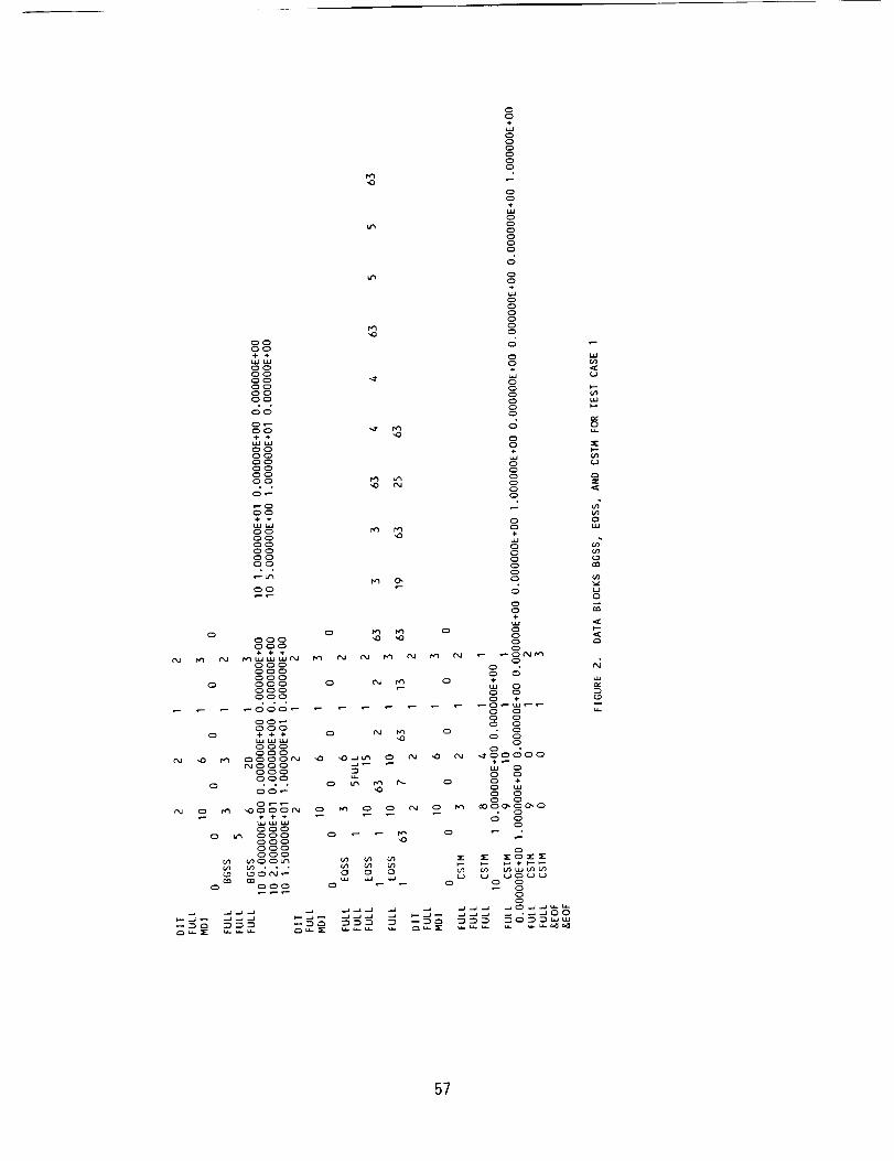
CDOOC)÷ 4.klJ_Oooooooooc3oo
wl._lc#.OC.{Dc.o
g°o
CDCD+ ÷
_CD(;DO
, °_u _,
_O
CD
÷
00000
C30
,t,
÷
N
÷
,0
÷
N
,o _
,13 +
N0
tel O, O
+
o o0o _ _ ooo0 o
ooo oooo o oooo o +
o ooo o _ooo - 8 N_00 _ ÷
_88 o °
oooooo _ o o
ooo_ o
0_ 0 0
- +++ .... 5 N
°°°
o
I.J
u,.
s--i,....-b5_.J
b00u.i
_0
b0
_4
c)
u.
57
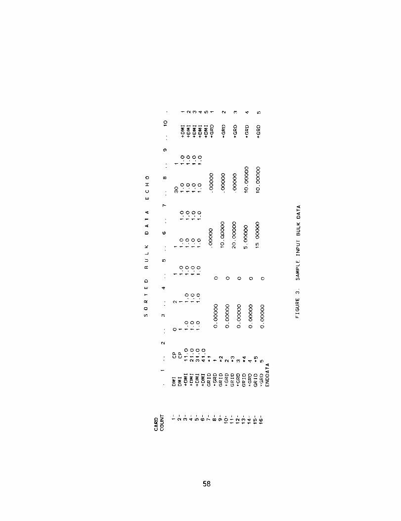
0
in
CO
(N
0000
0 0
+ooo88 8o08oo
oooo _ o o 6 60 ....
0000
o _ oo 80
ooo? 8 6 6 o
0000
0 0 0 0 0
000
000
0_
088800 0
o88§o8oo 86 6 6 6 5
0000_ ....
_ _ _ _ _ _ _._ _ _ _ _ _ _ _ Z_++++_*_*_+_
rll4111lllilllll
<0
58
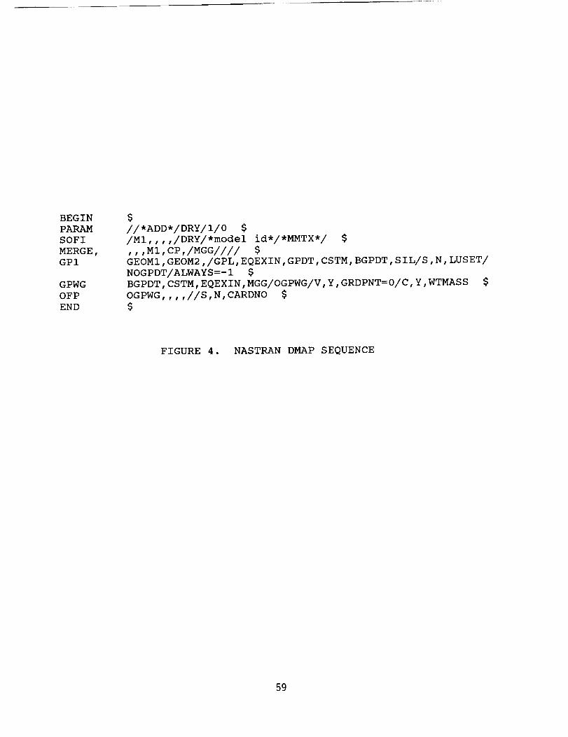
BEGIN
PARAM
SOFI
MERGE,GPI
GPWG
OFP
END
$//*ADD*/DRY/I/0 $
/MI,, , ,/DRY/*model id*/*MMTX*/ $
,,,MI,CP,/MGG//// $
GEOMI,GEOM2,/GPL,EQEXIN,GPDT,CSTM,BGPDT,SIL/S,N,LUSET/NOGPDT/ALWAYS=-I $
BGPDT,CSTM,EQEXIN,MGG/OGPWG/V,Y,GRDPNT=0/C,Y,WTMASS $
OGPWG,,,,//S,N,CARDNO $$
FIGURE 4. NASTRAN DMAP SEQUENCE
59
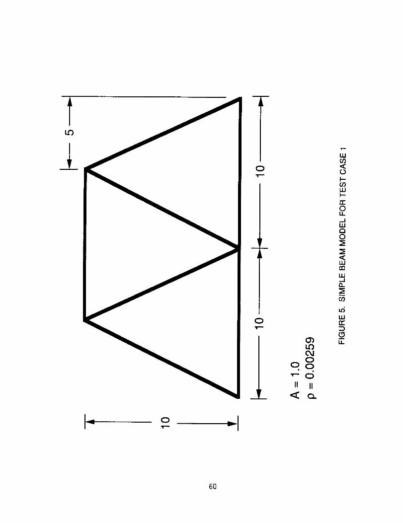
t!
O
O
_r
0O O
II II
W
,<
l-
Wp-n-OLI_,_IWa0
<WcO
W._.IO_
Wn-"
u_
O
6O
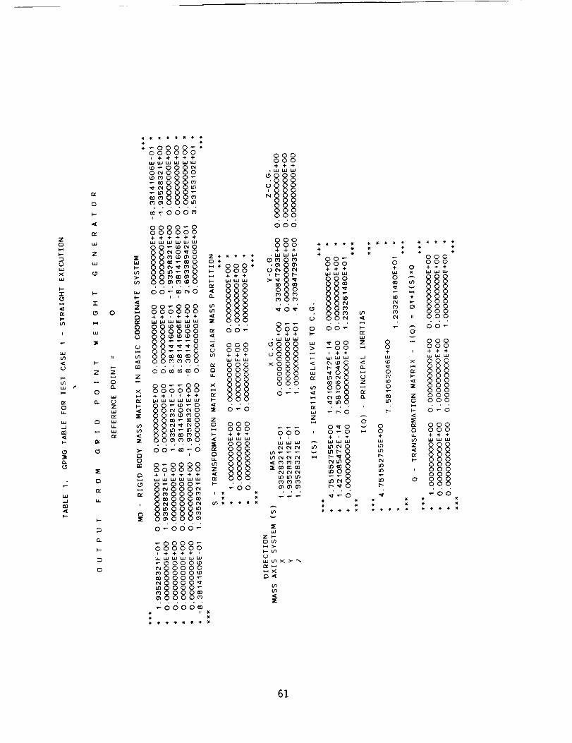
Z0
I--
-r
k--
i
i.u #'
0
..J
m
I..-
r,,
0
k-
u.I
Z
w
t.-
I
I--
Z
0
I3
0
0
11
Z
0e_
UZk,i¢,y
u.
wI--U')
Z
n¢
00
(J
U_
rn
Z
g
>.
O0
i
0
S8888s*i÷÷÷÷÷
°888;8o+÷÷÷÷+
i-00_0
°8S888w_w_w _ 000
o°_8gg8 _ oo-'''0
00_0 _ 000
08_0 _ 0000 _0 _ +++
00_0...... _ _00_0 0 000
, _ 000
0000
0_000_0
°8_.o o o§ _o ? 9§ _o
0 _ _0 w
...... _ 88o°°-_V° g 808
08 °0
°s8888o _ §_ _8+,÷+++__ _ 0
.oo6265dd
s8888;
_o 8oo8 _
_66666
uJZ_-O_
I.-v)
O0oo_+++
d66
888
0 0
0_000 0
• O0 >
_000
88s s °88+ + + + _' + + +
Z - :" o
_ _ g S
oo- _- - _ d6-:fv 0
_0 _ 0 O0
×ooo _< _§ _0_0 w0 0 _0000 _ _ 0 U000 _0
• '' _ 00_
0_ _ __
_0
z ?000 , 0_0
008
o _ _o_ O0_ O0
0 _ 800 O0Z 000
0 000
_ 6 S
0 _ 0000 0 000
+ _ ÷++
Z 000
_ O0
800
m o
4 '66
_N
_X
61
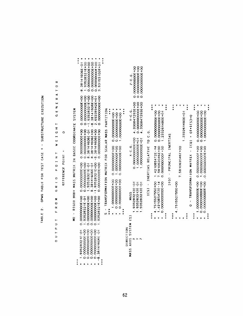
r_
0
Z
Zhl
W
F- I--
V) uJ
P 3
w _
m 0
k- Q.
0
._1
30. =E
0
m
0
0
Ii
Z
0
Z
¢Y
u./u..
l..-t_
>-
hiI--
Z
r_oo
o
nn
Z
b--
=£
=E
>-
0
ne
i
:E
*_0000_*000000
,+++++ 000
ooo0 ,ww_
-_ _ dggg_o- ,ogg_ o_°_ _gg °d2666d, 8@
8888;8 oo6÷+++÷+
O_ 00 O_ +
0_ _ +++ _
00_ _ _ w _ _
...... _ _i_ 0 _
00_0 _ Og 0 0
gg;ggg _÷+i+++
...000 _ 00_
00_ _ 00000_0 0 0 O0 '
00_0 _ +++ U
oo_o _ ,...... _00_0 0 0 0
, _ 000
°°--88 × °0000 000++,,++ _ 000
www_ww _ 00000_0 _ ,..
o°g_°o _ o-o00_0 Z
O_ _ 0 o 000o_-_o - ooo
...... . §§oO0_m_O _ 00 0 _
+_++++ _ 0 _
g _6_666_
;gggg; -_°_
_00000 __0000_ __0000 _ O__0000_
£6666di*
O0
O0++
+++
000 0 00_
ooo _ _go000 _ _ 0000 _ _++
g§o _ _0 _ _00 0 _ _0
000 w _00000 _ _0 U000 _0 Z
... _ 0000 _ _ _0
_0_0
000 , 0 _0 _ 0
4 '6 4
g ogg+ 0 + + +
_ M
g -
0
o ggg+ _ + + +UJ
'_ 0 0o _" ogo
© IE 0
00 ZIn 0 0
P- i-- 0_0
_" 0000 000u. + + +09 _.1 [.u LU
e_
0
0
62
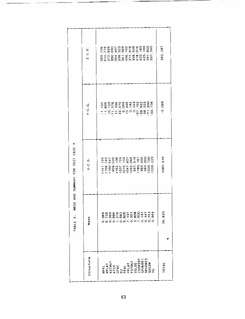
¢N
rD
t--
ilJt--
t",.
0U,..
>.
QZ
o'3
,g1.1.1
._Jrn
I-..
_DL
di
_r
I.
U
DI...
_0___0_
_0_0__0__0__0_
W6a6WW_W_WWWWIJ
__0__0_
_0___0___00__
_0__00_0
m_O__m_O00_
m__O_OOOm_O_Om--O0_O
_0__0___0__00_m_OOO__m
_66_6W_6_6666
0O
O_
0
c_i
0
_0
L_C_
.J
I--0
63
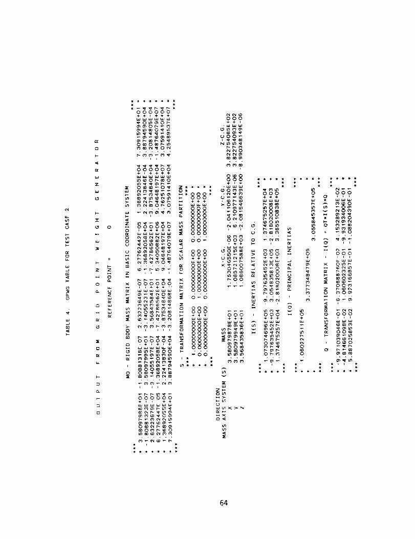
_P
F.-
0
(_0
4
0
n,
Z
I-
"1"
0
L_
3
Z
0
O.
n,
0
:E
0
0
II
7
0
ZL_
000000
++i+++_w_w_w_0_@0__0_
_0_
0_0__0_
000000
_0_0
0_0_
__ _ +++
000000I+++++
0 __ ----0 __ _ O0
__ _ 000
_0_ U 000
__ 0 O0Z ,, _ _ 000
. 000000_'+++'" 0__ _ 0
_0_ _ '''__ _ 0_0
__ 0 000_0_ _ O0 0__0 _ +++
_ I IIIo _000000
_oo _ .--O0
_00_
0 0__
000000
d2_2g
O* *
_,oo 8 .O0
.#
_r
000
._000_
_0
i
898
_0_._
>0_
_0 _
0_0
i i
000 0_++
_0_
000 0 000+++ + 0 Ill
0 _ __ _ * _0
_0_ _ _ _
_ _ 0 tl _0
i _ 0 II
000 -- 0 000_ _ +++
0_0 _ _0
_ _ _0 0_00 _ Z
''" _ _0
000 , 000 _ 0+++ +++ +
00_ _ 0
ddd _"
+ I III
00_
0 _0_
0 000
00_
, 0_0
* @
64
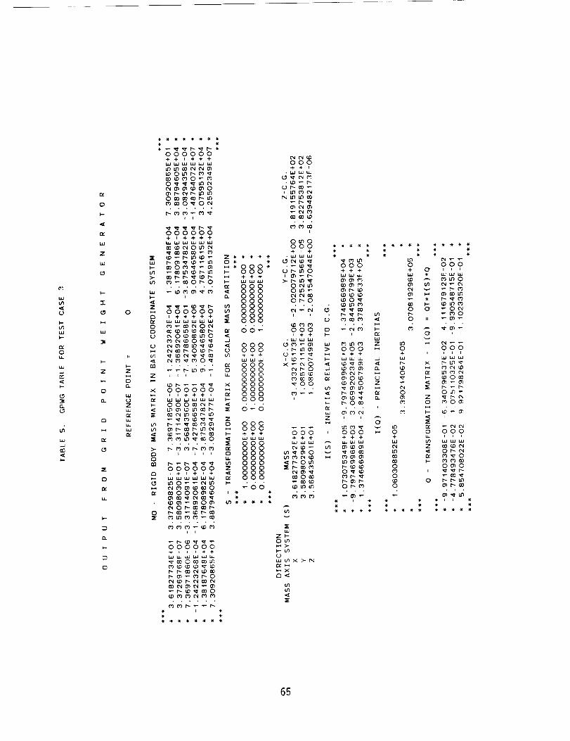
C)
uJ
I--
,-v
0
3_o_
.4
03
0
I.-
c[
w
Z
"r
iJJ
i..-
Z
0
r,
n,"
0
I,-..-
D
a.
I..-
0
0
_E
I-.-
>.
Z
,...,
0
0fO
r.O
Z
X
¢vI-.-
Ig
O0
n,
0
*******
000000++r+++
_0_0_
_gdJd4
000000
+1++++
__o_
000000
_0_
_0_0_0_
_0_
_0_
__ 0
000000
000_
Z * * * * *0 * *
Z*°8°*o o+ + +
I-- I_l 1.1.11._1
000000+ + +
000000000
000000000000
,_ , . ._ 0_0
Z
0 0_00 0F- + + +
__0 _ _
! §§oooooooo _ 8*+1+_+
_0_ _ ,.._m_O _00_000_ ,* *
_0_ _* * * * *_0_
000000
000++_
,_
N_
I
0_0
000 *_*** ***** **_**
* * * * * ** * * * * *
• _ 000_0 +++
0_ _
0_0 _0_
ooo o _
• _ > 000_ _ +++
_0 _ __0 _ _
_ _ _0__00 _0 Z
.., _ _
_0_
000 _ 000+++ +++
_ 0__0_ _
_ 0_
0
0+
o4u3
eO
0
0
0
0 000
+ 0 l,_
0 0 _0__0
0 000I Ill
0 mO_
d _ 4-e
0 000
0_
OmO
d45
Z_
k.-t_
O<
_9
u_<
:E
* i * * * .11 ** * * * * ****** ***** *****
65
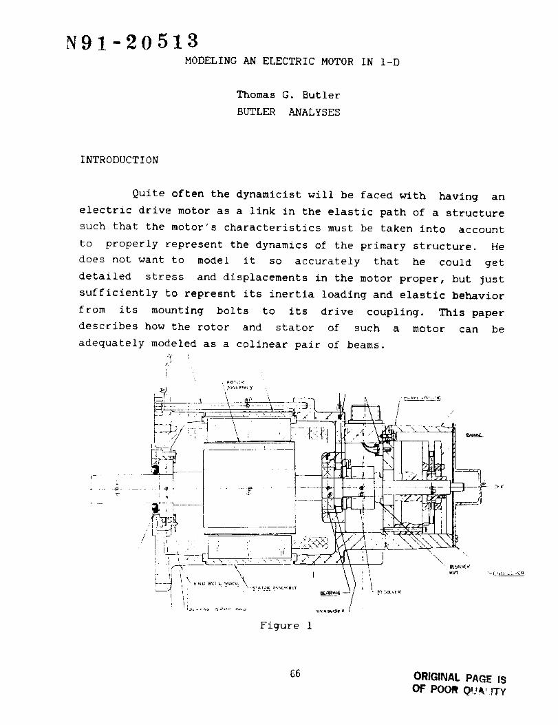
N91-20513MODELING AN ELECTRIC MOTOR IN I-D
Thomas G. Butler
BUTLER ANALYSES
INTRODUCTION
Quite often the dynamlcist will be faced with having an
electric drive motor as a link in the elastic path of a structure
such that the motor's characteristics must be taken into account
to properly represent the dynamics of the primary structure. He
does not want to model it so accurately that he could get
detailed stress and displacements in the motor proper, but just
sufficiently to represnt its inertia loading and elastic behavior
from its mounting bolts to its drive coupling. This paper
describes how the rotor and stator of such a motor can be
adequately modeled as a colinear pair of beams.
/
Figure 1
i
66 ORIGINAL PAGE IS
OF POOR Q!2_,_'!TY
MODELING AN ELECTRIC MOTOR IN 1 - D
PLAN
Figure 1 shows an assembly drawing of a motor equipped
with a disk brake. The application in which this motor was
incorporated required that the brake be set; consequently, the
electric coupling from the armature to the stator field was not
modeled. The discussion of the modeling will be taken up in four
parts: the rotor, the stator, the brake and the mount.
The overall scheme is to locate grid points at the
bearings, at the concentrations of mass, at the brake, and at the
mating interfaces. Six (6) grid points were assigned to the
rotor and 8 grid points were assigned to the stator. See Table i.
Between the grid points the structure undergoes several changes
of section. Each section is considered separately then the
stiffness for an equivalent prismatic bar is computed for the
sequence of sections between grid points.
One of the intriguing features about finite element
analysis is that parts can occupy the same physical location yet
can still remain disjoint. That feature will be employed here.
The stator is concentric with the rotor so the centroid of the
stator is coincident with the centroid of the rotor. Thus their
individual beam models will be colinear.
EQUIVALENCE
An example of one equivalent bar will be developed for
the rotor and another for the stator. The rotor between the bell
housing and the armature center of gravity has 3 separate sec-
tions: the bearing journal, intermediate shaft and armature.
The three sections are arrayed in line one after the other. This
is an elastic series situation so equivalence is found by summing
compliances (Z). The formulas for equivalent area and equivalent
bending inertia are:
67
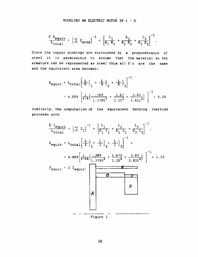
MODELING AN ELECTRIC MOTOR IN 1 - D
EA
eguiv = (_ Zarea)r'tota 1 -I [ L 1 L 2 L33 ]
-i
Since the copper windings are surrounded by a preponderance of
steel it is permissible to assume that the material in the
armature can be represented as steel thus all E's are the same
and the equivalent area becomes:
-I
[÷I•÷I•÷I]Aequiv Lt°tal 1 2 3
-I
[±I .389 1.6___/7. 2:83)]= 4.889 [_/4 1.37852 + 2.252 3.8312= 5.28
Similarly, the computation of the equivalent bending inertias
proceeds with
-i
I L2E Ie_ui v Z Z I II 2- = + +
Ltota 1 E 2 I E 3 I
-1
[+I+ ÷I]Iequiv Lt°tal 1 3
Jequiv
[_i-7_( :38_/9= 4.889 1.37854
= 2 Iequiv"
A
B
1.670
2.254
-1
3. 8314
w
Figure 2
Q
l°
68
MODELING AN ELECTRIC MOTOR IN 1 - D
The approach to equivalent properties for the stator is
similar to that for the rotor except that the sections are not
solid, the array is partially in parallel and partially in se-
ries, and it involves distinct materials, as seen in Figure 2.
Note that sections C & D act in parallel; therefore the net
combined stiffness "K" is KCD = KC+ KD, and the net compliance is
ZCD = I/KcD. Section B acts in series with the CD combination,
therefore the net combined compliance is ZBC D = Z B + ZCD.
Section E acts in parallel with the inner combination of BCD,
therefore the net elasticity is obtained by adding stiffnesses.-I
KBCDE = KE + KBC D = K E + ZBC D and ZBCDE = I/KBcDE. Finally,
section A acts in series with the combined sections BCDE; i.e.
Zne t = ZA + ZBCDE. The equivalent sectional properties can be
obtained from Zne t. The numerical statistics for the components
of this stator bar example are given in Table 3. Use of these
data in the combining formulas is carried out just for stator
equivalent area as follows.
CD C D 2.689 +
7/4(6.752- 4.582 ) 3 x 107=
2.689
_x107 ( )= 4 x 2?689 5.132 + 3 x 24.586 = 2.304 x 10⁸ .
zareaCD = 4.340 x 10 -9
Combining item B in series with the CD combination gives
_area _area _area LB _area-- + :
-BCD = _B + -CD ABEal -CD
= 2.007 + 4.34 x i0 -9= 2.526 x i0 -8
g/4(7.382- 6.52 ) x 107
-1
( area I : 3.95 x i07warea = ZBC D_'BCD
Item E combines in parallel with item BCD.
_area 4(_/4)(5/16)2x 3 x i0'
mBCDE = 4.53+ 3.958 x 107 = 4.162 x 10⁷
69
MODELING AN ELECTRIC MOTOR IN 1 - D
-i
zarea I. area_BCDE = _BCDE) = 2.403 x 10 -8
And now section A can be combined in series
result.
with the current
LA 0.62zarea = _area _net AA_a + mBCDE
(7.52- _ 2/852 ) x 107
= 2.567 x 10 -8 = Lt°tal
EalAequiv
Eal
Aequi v = zare a = 19.347.Ltotal net
+ 2.403 x 10 -8
Similar calculations yield equivalent area
Iequi v as was shown for the rotor bar example.
COLLATERAL
moment of inertia
These operations were performed for the rest of the rotor
and stator. This completes the complement of properties for
equivalent prismatic bars. It will be mentioned, only in pass-
ing, that the mass can be well modeled automatically (except for
torsional inertias) by calling for COUPMASS. The assignment of
torsional mass moment of inertia per grid point must be manually
determined and entered as CMASS2 elements. The next topic
concerns the mating of the rotor to the stator at the bearings.
This motor was designed with ball bearings which can absorb
thrust. Therefore, the two bearings link the rotor and stator
without connecting any rotations. This was represented as
Multi-Point-Constraints (MPC's) in all 3 translations, between
the two rotor bearing points, numbers 2 & 4 and the corresponding
stator points, numbers 30 & 33.
brake.
The topic that needed particular study was the disc
The following discussion will refer to Figure 3.
7O
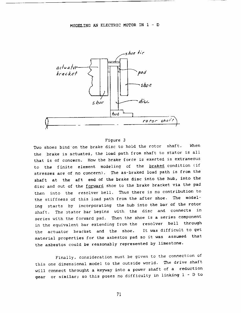
MODELING AN ELECTRIC MOTOR IN 1 - D
i !
i
I
)Ii
5 ]Tpr
- pad
t_O /-or" #h,ai-'k_
J
Figure 3
Two shoes bind'on the brake disc to hold the rotor shaft. When
the brake is actuated, the load path from shaft to stator is all
that is of concern. How the brake force is exerted is extraneous
to the finite element modeling of the braked condition (if
stresses are of no concern). The as-braked load path is from the
shaft at the aft end of the brake disc into the hub, into the
disc and out of the forward shoe to the brake bracket via the pad
then into the resolver bell. Thus there is no contribution to
the stiffness of this load path from the after shoe. The model-
ing starts by incorporating the hub into the bar of the rotor
shaft. The stator bar begins with the disc and connects in
series with the forward pad. Then the shoe is a series component
in the equivalent bar extending from the resolver bell through
the actuator bracket and the shoe. It was difficult to get
material properties for the asbestos pad so it was assumed that
the asbestos could be reasonably represented by limestone.
Finally, consideration must be given to the connection of
this one dimensional model to the outside world. The drive shaft
will connect throught a keyway into a power shaft of a reduction
gear or similar; so this poses no difficulty in linking 1 - D to
71
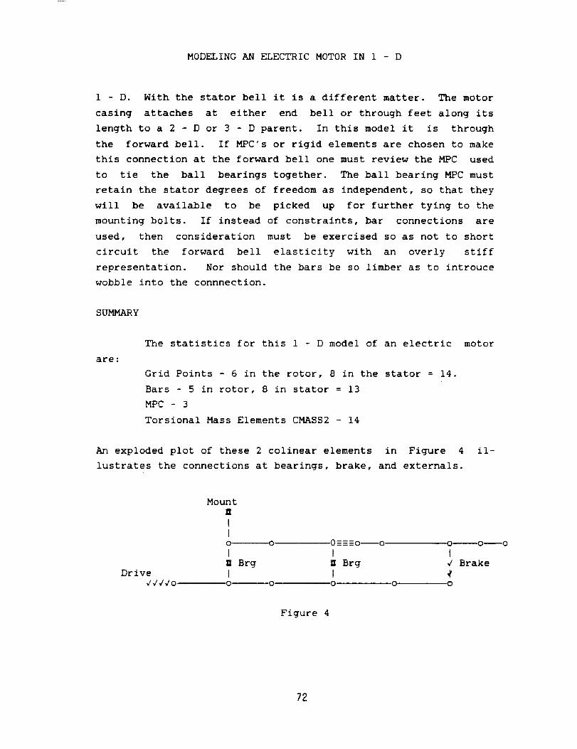
MODELING AN ELECTRIC MOTOR IN 1 - D
1 - D. With the stator bell it is a different matter. The motor
casing attaches at either end bell or through feet along its
length to a 2 - D or 3 - D parent. In this model it is through
the forward bell. If MPC's or rigid elements are chosen to make
this connection at the forward bell one must review the MPC used
to tie the ball bearings together. The ball bearing MPC must
retain the stator degrees of freedom as independent, so that they
will be available to be picked up for further tying to the
mounting bolts. If instead of constraints, bar connections are
used, then consideration must be exercised so as not to short
circuit the forward bell elasticity with an overly stiff
representation. Nor should the bars be so limber as to introuce
wobble into the connnection.
SUMMARY
are:
The statistics for this 1 - D model of an electric
Grid Points - 6 in the rotor, 8 in the stator = 14.
Bars - 5 in rotor, 8 in stator = 13
MPC - 3
Torsional Mass Elements CMASS2 - 14
motor
An exploded plot of these 2 colinear elements in Figure 4 il-
lustrates the connections at bearings, brake, and externals.
Mount
U
II
o o 0_o--o
I IU Brg H Brg
Drive I I444_o ,o o o .o
0--0--0
t4 Brake
o
Figure 4
72

MODELING AN ELECTRIC MOTOR IN 1 - D
CONCLUSION
It has been shown that the necessary characteristics of
an electric motor can be incorporated into a dynamic model by
means of a lean bar model without having to resort to a full
blown three dimensional model.
73
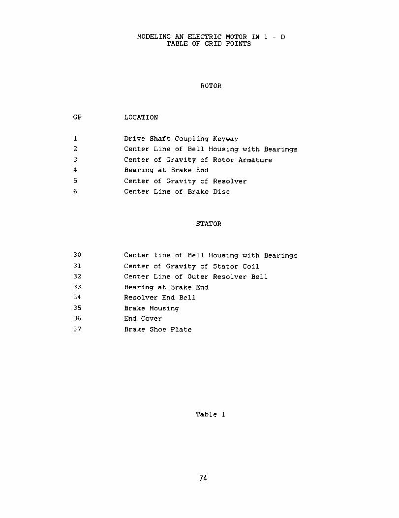
MODELING AN ELECTRIC MOTOR IN 1 - DTABLE OF GRID POINTS
ROTOR
GP LOCATION
1
2
3
4
5
6
Drive Shaft Coupling Keyway
Center Line of Bell Housing with Bearings
Center of Gravity of Rotor Armature
Bearing at Brake End
Center of Gravity of Resolver
Center Line of Brake Disc
STATOR
3O
31
32
33
34
35
36
37
Center line of Bell Housing with Bearings
Center of Gravity of Stator Coil
Center Line of Outer Resolver Bell
Bearing at Brake End
Resolver End Bell
Brake Housing
End Cover
Brake Shoe Plate
Table 1
74
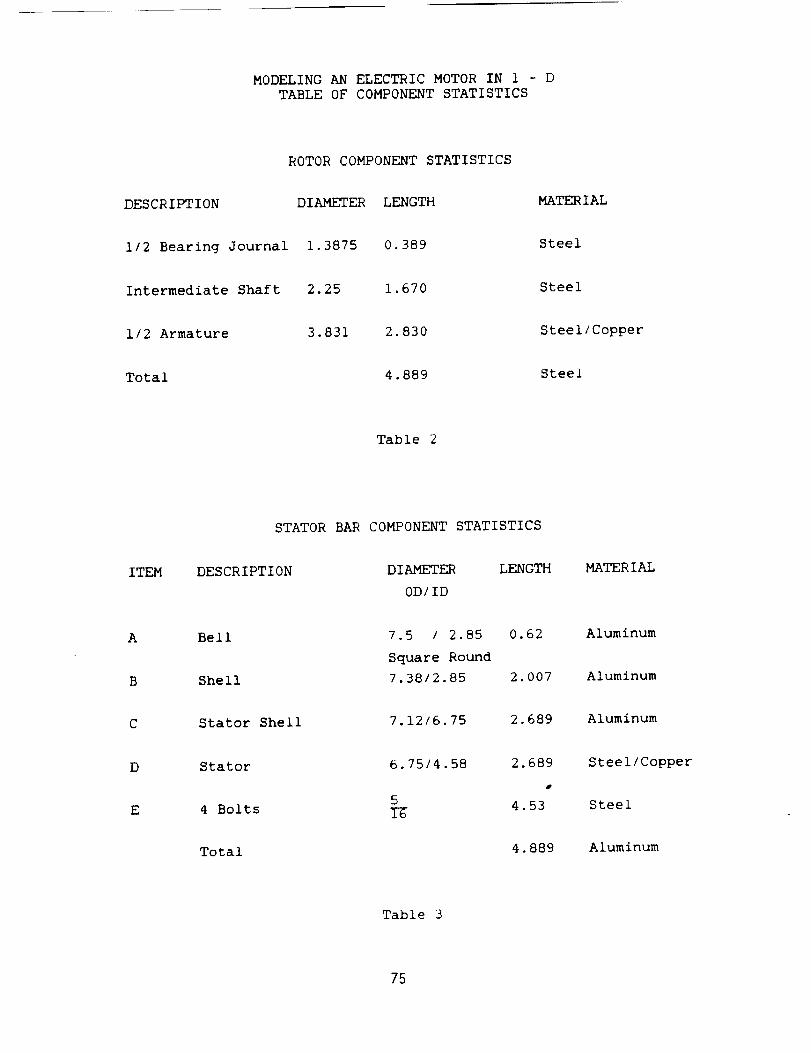
MODELING AN ELECTRIC MOTOR IN 1 - D
TABLE OF COMPONENT STATISTICS
ROTOR COMPONENT STATISTICS
DESCRIPTION DIAMETER LENGTH MATER IAL
1/2 Bearing Journal 1.3875 0.389 Steel
Intermediate Shaft 2.25 1.670 Steel
1/2 Armature 3.831 2.830 Steel/Copper
Total 4.889 Steel
Table 2
STATOR BAR COMPONENT STATISTICS
ITEM DESCRIPTION DIAMETER
0D/ID
LENGTH MATERIAL
A Bell
B Shell
7.5 / 2.85 0.62
Square Round
7.38/2.85 2.007
Aluminum
Aluminum
C Stator Shell 7.12/6.75 2.689 Aluminum
D
E
Stator
4 Bolts
Total
6.75/4.58
5I-6
2.689 Steel/Copper
4.53 Steel
4.889 Aluminum
Table 3
75
N9 _-20514COMPUTER ANIMATION OF NASTRAN DISPLACEMENTS
ON IRIS 4D-SERIES WORKSTATIONS:
CANDI/ANIMATE POSTPROCESSING OF NASHUA RESULTS
Janine L. Fales
Los Alamos National Laboratory
Advanced Engineering Technology (MEE-13)
Los Alamos, New Mexico 87545
SUMMARY
The capabilities of the postprocessing program CANDI (Color
Animation of Nastran Displacements) [1] have been
expanded to accept results from axisymmetric analyses. An
auxiliary program, ANIMATE, has been developed to allow
color display of CANDI output on the IRIS 4D-series
workstations. The user can interactively manipulate the
graphics display by three-dimensional rotations, translations,
and scaling through the use of the keyboard and/or dials box.
The user can also specify what portion of the model is
displayed. These developments are limited to the display of
complex displacements calculated with the
NASHUA/NASTRAN procedure for structural acoustics
analyses [2].
INTRODUCTION
Animation of results has become an increasingly popular method of
postprocessing because of the wealth of information conveyed to the
analyst in a short amount of time. Animation allows the analyst to
visualize time-dependent results that previously could only be
imagined from a series of static plots. Through animation, the
analyst is able to focus on the interpretation of the results, having
been freed from the burden of envisioning their time dependency.
The advantages of animation were recognized by Lipman at David
Taylor Research Center (DTRC), in the development of the
postprocessing computer program, CANDI (Color Animation of
Nastran Displacements) [1]. CANDI was originally written to
76
interface with an Evans & Sutherland PS-330 interactive graphicssystem [3] for the graphics display. Unfortunately, the usefulness ofCANDI was limited to those with access to this specific hardware.
A postprocessing tool was required for displaying complexdisplacements obtained with the NASHUA/NASTRAN procedure(hereafter referred to as NASHUA). NASHUA, developed byEverstine and Quezon at DTRC, is a coupled finite element/boundaryelement capability built around NASTRAN for calculating the low-frequency, far-field acoustic pressure field radiated or scattered byan arbitrary, submerged, elastic structure subjected to eitherinternal, time-harmonic, mechanical loads or external, time-harmonic, incident loadings [2]. The structure can be axisymmetricor three-dimensional. CANDI was one postprocessing option forthree-dimensional NASHUA analyses. An axisymmetric tool was alsorequired.
Rather than replicate the work of Lipman, an auxiliary computerprogram, ANIMATE, was developed to accept, as input, the output
from CANDI and display the results on the IRIS 4D-series
workstations, manufactured by Silicon Graphics, Incorporated (SGI).
The choice of the IRIS workstation was based on its three-
dimensional, graphics display capabilities. CANDI was also expanded
to postprocess results from axisymmetric NASHUA analyses.
Because the work described here was done to accomplish specific,
programmatic needs, the scope of the computer program developed
is limited to the display of complex displacements calculated with
NASHUA. Although CANDI is able to postprocess results from other
types of analyses, there are no expectations on the part of the authorto enable ANIMATE to display these results. It is hoped that the
foundations of the program are sound enough to allow enhancements
by others, if needed.
THE NASHUA/NASTRAN PROCEDURE (NASHUA)
The NASHUA/NASTRAN procedure, also called the NASHUA
capability or NASHUA, is explained, in detail, in Ref. 2. At Los
Alamos National Laboratory, NASHUA is executed on a Cray
supercomputer running under a CTSS operating system. Table 1
summarizes the steps involved in this type of analysis. Rigid Format
8 (direct frequency response) is used for each NASTRAN execution.
All DMAP ALTER sequences are given in Ref. 2. The DMAP ALTER
77
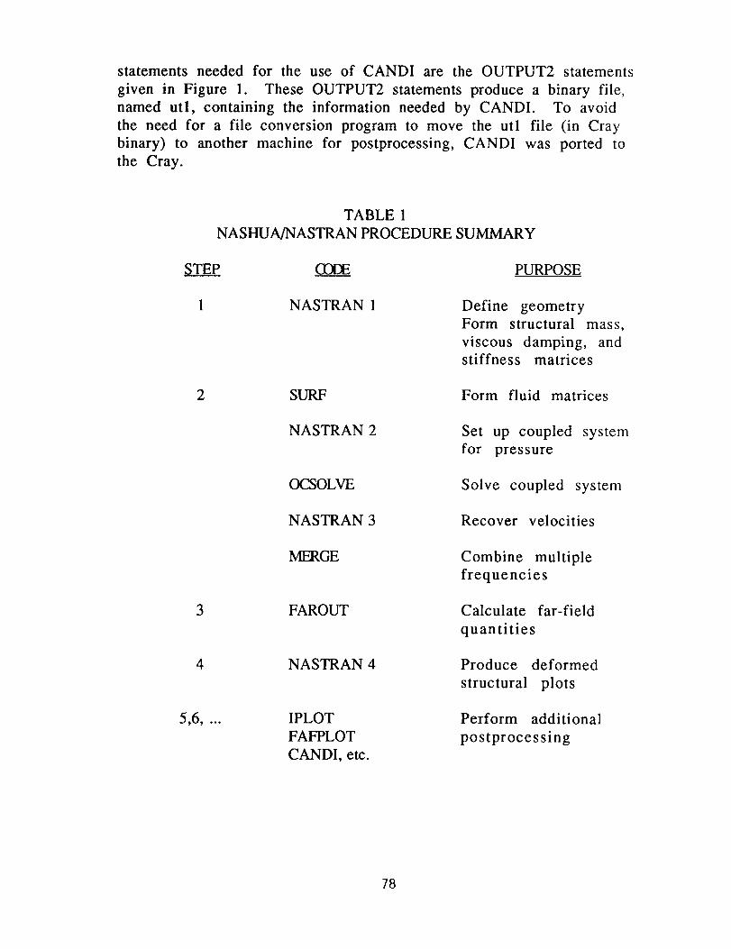
statements needed for the use of CANDI are the OUTPUT2 statements
given in Figure 1. These OUTPUT2 statements produce a binary file,
named utl, containing the information needed by CANDI. To avoid
the need for a file conversion program to move the utl file (in Cray
binary) to another machine for postprocessing, CANDI was ported to
the Cray.
TABLE 1
NASHUA/NASTRAN PROCEDURE SUMMARY
STEP (33[_
1 NASTRAN 1
2
3
4
SURF
NASTRAN 2
(X_OLVE
NASTRAN 3
MERGE
FAROUT
NASTRAN 4
IPLOT
FAFPLOT
CANDI, etc.
596, ooo
PURPOSE
Define geometry
Form structural mass,
viscous damping, andstiffness matrices
Form fluid matrices
Set up coupled system
for pressure
Solve coupled system
Recover velocities
Combine multiple
frequencies
Calculate far-field
quantities
Produce deformed
structural plots
Perform additional
postprocessing
78
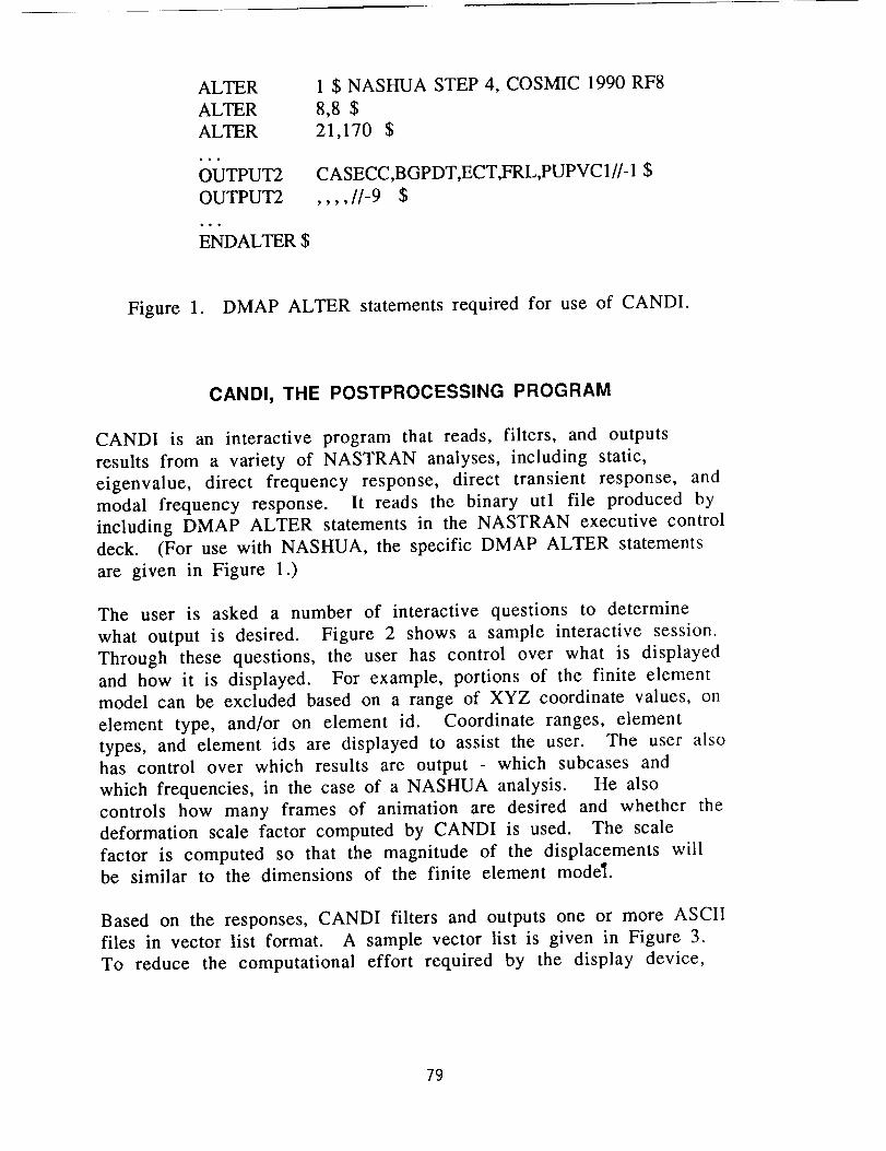
ALTERALTERALTER• ! •
OUTPUT2
OUTPUT2
ENDALTER $
1 $ NASHUA STEP 4, COSMIC 1990 RF8
8,8 $
21,170 $
CASECC,BGPDT,ECT,FRL,PUPVC1//- 1 $
,,,,//-9 $
Figure 1. DMAP ALTER statements required for use of CANDI.
CANDI, THE POSTPROCESSING PROGRAM
CANDI is an interactive program that reads, filters, and outputs
results from a variety of NASTRAN analyses, including static,
eigenvalue, direct frequency response, direct transient response, and
modal frequency response. It reads the binary utl file produced by
including DMAP ALTER statements in the NASTRAN executive control
deck. (For use with NASHUA, the specific DMAP ALTER statements
are given in Figure 1.)
The user is asked a number of interactive questions to determine
what output is desired. Figure 2 shows a sample interactive session.
Through these questions, the user has control over what is displayed
and how it is displayed. For example, portions of the finite element
model can be excluded based on a range of XYZ coordinate values, on
element type, and/or on element id. Coordinate ranges, element
types, and element ids are displayed to assist the user. The user also
has control over which results are output which subcases and
which frequencies, in the case of a NASHUA analysis. He also
controls how many frames of animation are desired and whether the
deformation scale factor computed by CANDI is used. The scale
factor is computed so that the magnitude of the displacements willbe similar to the dimensions of the finite element model.
Based on the responses, CANDI filters and outputs one or more ASCII
files in vector list format. A sample vector list is given in Figure 3.
To reduce the computational effort required by the display device,
79
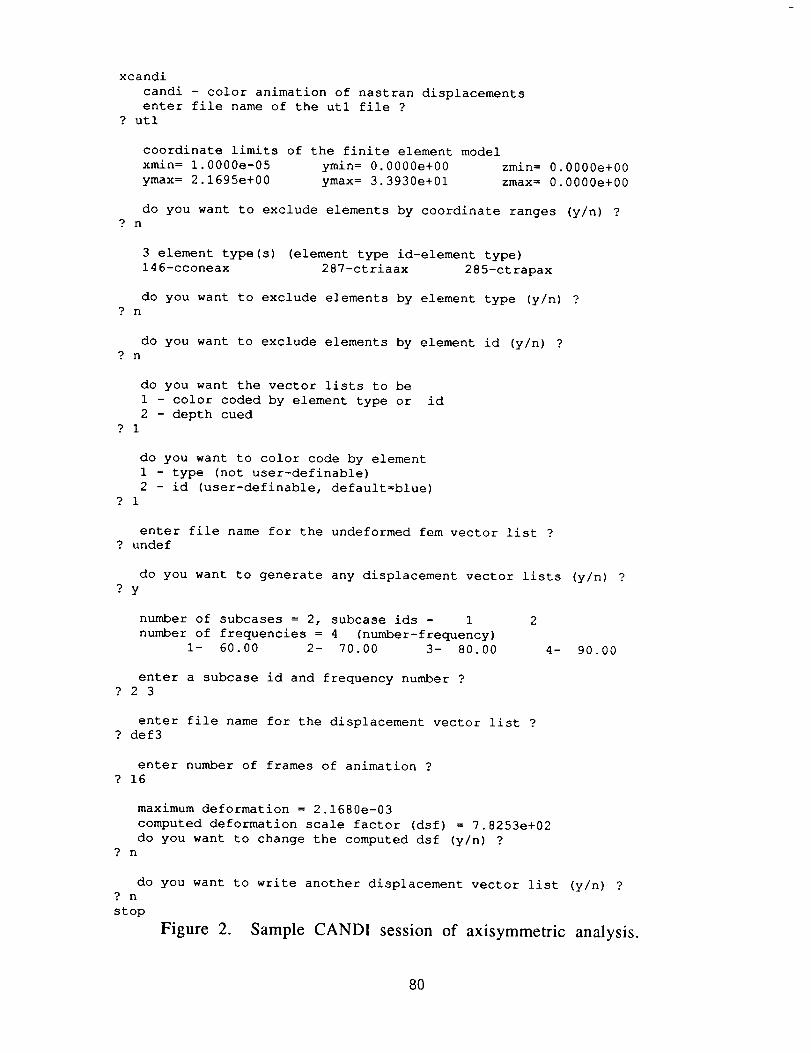
xcandi
candi - color animation of nastran displacements
enter file name of the utl file ?
? utl
coordinate limits of the finite element model
xmin= l. O000e-05 ymin= O.O000e+O0 zmin= O.O000e+O0
ymax= 2.1695e+00 ymax= 3.3930e+01 zmax= O.O000e+O0
do you want to exclude elements by coordinate ranges (y/n) ??n
3 element type(s) (element type id-element type)
146-cconeax 287-ctriaax 285-ctrapax
do you want to exclude elements by element type (y/n) ??n
do you want to exclude elements by element id (y/n) 9? n
do you want the vector lists to be
1 - color coded by element type or id
2 - depth cued? 1
do you want to color code by element
1 - type (not user-definable)
2- id (user-definable, default=blue)? 1
enter file name for the undeformed fem vector list
undef
do you want to generate any displacement vector lists (y/n) ??y
number of subcases = 2, subcase ids - 1 2
number of frequencies = 4 (number-frequency)
I- 60.00 2- 70.00 3- 80.00 4- 90.00
enter a subcase id and frequency number ?? 2 3
enter file name for the displacement vector list? def3
enter number of frames of animation ?
? 16
maximum deformation = 2.1680e-03
computed deformation scale factor (dsf) = 7.8253e+02
do you want to change the computed dsf (y/n) ?? n
do you want to write another displacement vector list (y/n) ?? n
stop
Figure 2. Sample CANDI session of axisymmetric analysis.
8O
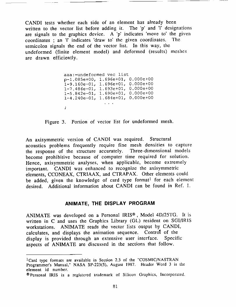
CANDI tests whether each side of an element has already been
written to the vector list before adding it. The 'p' and T designations
are signals to the graphics device. A 'p' indicates 'move to' the given
coordinates ; an T indicates 'draw to' the given coordinates. The
semicolon signals the end of the vector list. In this way, the
undeformed (finite element model) and deformed (results) meshes
are drawn efficiently.
aaa =undeformed vec list
p-I 085e+00, 1.696e+01, O.O00e+O0
1-9 160e-Ol, 1.696e+01, O.O00e+O0
1-7 486e-01, 1.693e+01, O.O00e+O0
1-5 842e-01, 1.690e+01, O.O00e+O0
1-4 240e-01, 1.684e+01, O.O00e+O0
Figure 3. Portion of vector list for undeformed mesh.
An axisymmetric version of CANDI was required. Structural
acoustics problems frequently require fine mesh densities to capture
the response of the structure accurately. Three-dimensional models
become prohibitive because of computer time required for solution.
Hence, axisymmetric analyses, when applicable, become extremely
important. CANDI was enhanced to recognize the axisymmetric
elements, CCONEAX, CTRIAAX, and CTRAPAX. Other elements could
be added, given the knowledge of card type format 1 for each elementdesired. Additional information about CANDI can be found in Ref. 1.
ANIMATE, THE DISPLAY PROGRAM
ANIMATE was developed on a Personal IRIS ® , Model 4D/25TG. It is
written in C and uses the Graphics Library (GL) resident on SGI/IRIS
workstations. ANIMATE reads the vector lists output by CANDI,
calculates, and displays the animation sequence. ControI of the
display is provided through an extensive user interface. Specific
aspects of ANIMATE are discussed in the sections that follow.
1Card type formats are available in Section 2.3 of the "COSMIC/NASTRAN
Programmer's Manual," NASA SP-223(5), August 1987. Header Word 3 is theelement id number.
®Personal IRIS is a registered trademark of Silicon Graphics, Incorporated.
81
HARDWARE / SOFTWARE REQUIREMENTS
The Personal IRIS, Model 4D/25 TG, on which ANIMATE was
developed, was originally purchased for its three-dimensional
capabilities with PATRAN ®. The Personal IRIS (4D/20+) series give
favorable price/performance curves. The need to animate complex
displacements spearheaded the effort to port CANDI to the IRIS
platform. In addition, other postprocessing tools for structural
acoustics analyses had been developed for the IRIS 4D-series
workstations.
The high-level Graphics Library made the graphics programming
relatively easy. However, because the GL was used, ANIMATE is not
universally portable. It is only portable to IRIS 4D-series
workstations, or to IBM machines on which the GL has been installed.
The IRIS Window Manager, based on the NeWS server environment
was used to develop the user interface.
ANIMATE was initially developed using the dials box for the three-
dimensional rotations, translations, and scaling. While the dial box is
an intuitive method to accomplish these transformations, it is an
optional peripheral. Therefore, the same functionality was tied to
keys found on the standard IRIS keyboard. If available, use of the
dial box is preferred.
The minimum hardware requirement to use ANIMATE is an IRIS
4D/20 G workstation. Any graphics workstation of the 4D-series is
acceptable. The dial box is useful, but optional.
OALCULATION OF ANIMATION SEQUENCE
Animation of the harmonic time dependence of the complex
displacements is accomplished according to the following equation.
F i = V u + DSF [ VRe cos0i - Vim sin0i ]
where F i =
V u =
VRe =
Vim =
ith frame of animation,
undeformed vector list,
vector list of real components,
vector list of imaginary components,
®PATRAN is a registered trademark of PDA Engineering.
82
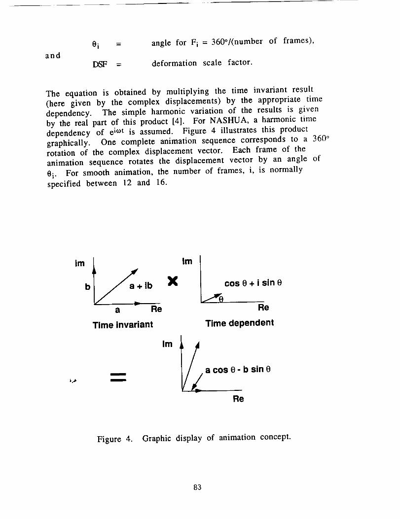
and
0 i =
DSF -
angle for F i = 360°/(number of frames),
deformation scale factor.
The equation is obtained by multiplying the time invariant result
(here given by the complex displacements) by the appropriate time
dependency. The simple harmonic variation of the results is given
by the real part of this product [4]. For NASHUA, a harmonic time
dependency of e it0t is assumed. Figure 4 illustrates this product
graphically. One complete animation sequence corresponds to a 360 °
rotation of the complex displacement vector. Each frame of the
animation sequence rotates the displacement vector by an angle of
0 i. For smooth animation, the number of frames, i, is normally
specified between 12 and 16.
Im
b+ib X
a Re
Time invariant
Im
7ocos 0 + i sin 0
Re
m
;_jb mmlv//_
Time dependent
a cos 0 - b sin 0
Re
Figure 4. Graphic display of animation concept.
83
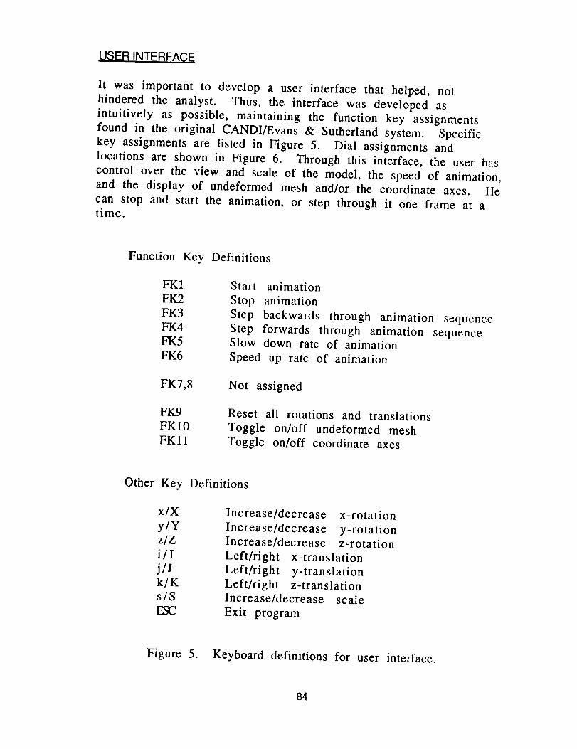
VSER INTERFACE
It was important to develop a user interface that helped, not
hindered the analyst. Thus, the interface was developed as
intuitively as possible, maintaining the function key assignments
found in the original CANDI/Evans & Sutherland system. Specific
key assignments are listed in Figure 5. Dial assignments and
locations are shown in Figure 6. Through this interface, the user has
control over the view and scale of the model, the speed of animation,
and the display of undeformed mesh and/or the coordinate axes. He
can stop and start the animation, or step through it one frame at atime.
Function Key Definitions
FK1
FK2
FK3
FK4
FK5
FK6
Start animation
Stop animation
Step backwards through animation sequence
Step forwards through animation sequenceSlow down rate of animation
Speed up rate of animation
FK7,8 Not assigned
FK9
FK10
FK11
Reset all rotations and translations
Toggle on/off undeformed mesh
Toggle on/off coordinate axes
Other Key Definitions
x/X
y/Y
z/Z
i/I
j/J
k/K
s/S
ESC
Increase/decrease x-rotation
Increase/decrease y-rotation
Increase/decrease z-rotation
Left/right x-translation
Left/right y-translation
Left/right z-translation
Increase/decrease scale
Exit program
Figure 5. Keyboard definitions for user interface.
84
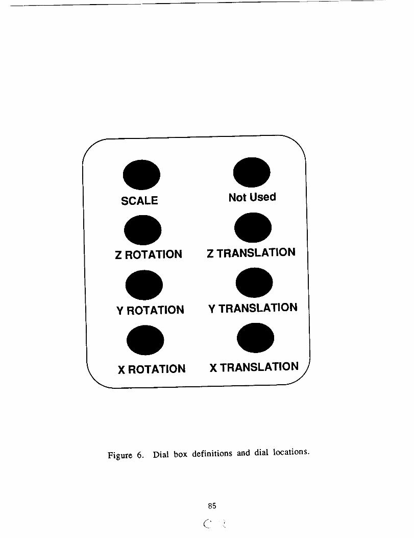
SCALE Not Used
\
Z ROTATION
Y ROTATION
X ROTATION
Z TRANSLATION
Y TRANSLATION
OX TRANSLATIONj
Figure 6. Dial box definitions and dial locations.
85
REFERENCES
• R. R. Lipman, "Computer Animation of Modal and Transient
Vibrations," Fifteenth NASTRAN Users' Colloquium, NASA CP-
2481, National Aeronautics and Space Administration,
Washington, D.C., pp 88-97 (May 1987).
. G. C. Everstine and A. J. Quezon, "User's Guide to the Coupled
NASTRAN/Helmholtz Equation Capability (NASHUA) for Acoustic
Radiation and Scattering," Third Ed., DTRC report CMLD-88/03
(February 1988).
o "PS-300 User's Manual," Evans & Sutherland Computer
Corporation, Salt Lake City, Utah, 1985.
. F. Fahy, Sound and Str0¢tural Vibration, Radiation, Transmission
and Response, Academic Press, 1985.
86
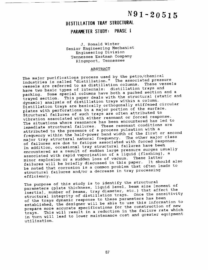
N91-20515DISTILLATION TRAY STRUCTURAL
PARAHETERSTUDY: PHASE I
J. Ronald Winter
Senior Engineering Mechanist
Engineering Division
Tennessee Eastman Company
Kingsport, Tennessee
ABSTRACT
The major purifications process used by the petro/chemical
industries is called "distillation." The associated pressure
vessels are referred to as distillation columns. These vessels
have two basic types of internals: distillation trays and
packing. Some special columns have both a packed section and a
trayed section. This paper deals with the structural (static and
dynamic) analysis of distillation trays within a column.
Distillation trays are basically orthogonally stiffened circular
plates with perforations in a major portion of the surface.
Structural failures of such trays are often attributed to
vibration associated with either resonant or forced response.
The situations where resonance has been encountered has led to
immediate structural failures. These resonant conditions are
attributed to the presence of a process pulsation with a
frequency within the half-power band width of the first or second
major tray structural natural frequency. The other major class
of failures are due to fatigue associated with forced response.
In addition, occasional tray structural failures have been
encountered as a result of sudden large pressure surges usually
associated with rapid vaporization of a liquid (flashing), a
minor explosion or a sudden loss of vacuum. These latter
failures will be briefly discussed in this paper. It should also
be noted that corrosion is a common problem that often leads to
structural failures and/or a decrease in tray processing
efficiency.
The purpose of this study is to identify the structural
parameters (plate thickness, liquid level, beam size [moment of
inertia], number of beams, tray diameter, etc.) that affect the
structural integrity of distillation trays. Once the sensitivity
of the trays dynamic response to these parameters has been
established, the designer will be able to use this information to
prepare more accurate specifications for the construction of new
trays. This will result in a reduction in the failure rate which
in turn will lead to lower maintenance cost and greater equipment
utilization.
87
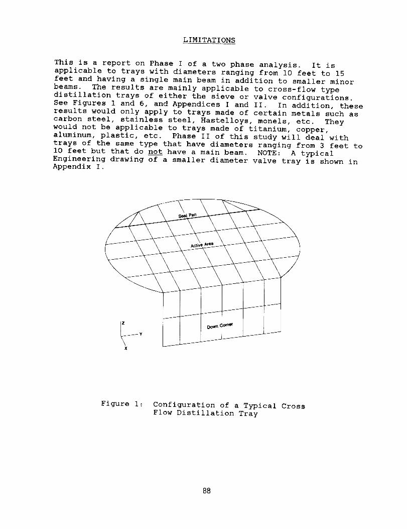
LIMITATIONS
This is a report on Phase I of a two phase analysis. It is
applicable to trays with diameters ranging from I0 feet to 15
feet and having a single main beam in addition to smaller minor
beams. The results are mainly applicable to cross-flow type
distillation trays of either the sieve or valve configurations.
See Figures 1 and 6, and Appendices I and II. In addition, these
results would only apply to trays made of certain metals such as
carbon steel, stainless steel, Hastelloys, monels, etc. They
would not be applicable to trays made of titanium, copper,
aluminum, plastic, etc. Phase II of this study will deal with
trays of the same type that have diameters ranging from 3 feet to
I0 feet but that do not have a main beam. NOTE: A typical
Engineering drawing of a smaller diameter valve tray is shown in
Appendix I.
X
Figure I: Configuration of a Typical Cross
Flow Distillation Tray
88
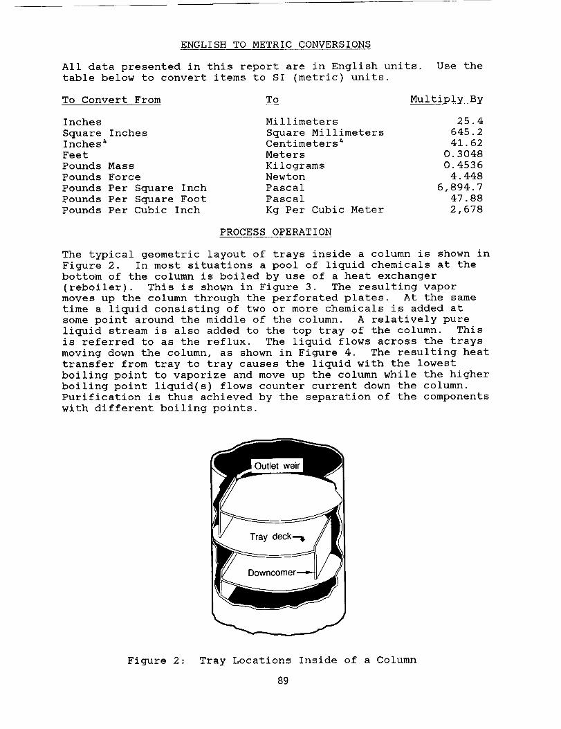
ENGLISH TO METRIC CONVERSIONS
All data presented in this report are in English units.
table below to convert items to SI (metric) units.
Use the
To Convert From To Multiply By
Inches
Square InchesInches _
Feet
Pounds Mass
Pounds Force
Pounds Per Square Inch
Pounds Per Square Foot
Pounds Per Cubic Inch
Millimeters 25.4
Square Millimeters 645.2Centimeters 4 41.62
Meters 0.3048
Kilograms 0.4536Newton 4.448
Pascal 6,894.7
Pascal 47.88
Kg Per Cubic Meter 2,678
PROCESS OPERATION
The typical geometric layout of trays inside a column is shown in
Figure 2. In most situations a pool of liquid chemicals at the
bottom of the column is boiled by use of a heat exchanger
(reboiler). This is shown in Figure 3. The resulting vapor
moves up the column through the perforated plates. At the same
time a liquid consisting of two or more chemicals is added at
some point around the middle of the column. A relatively pure
liquid stream is also added to the top tray of the column. This
is referred to as the reflux. The liquid flows across the trays
moving down the column, as shown in Figure 4. The resulting heat
transfer from tray to tray causes the liquid with the lowest
boiling point to vaporize and move up the column while the higher
boiling point liquid(s) flows counter current down the column.
Purification is thus achieved by the separation of the components
with different boiling points.
Figure 2: Tray Locations Inside of a Column
89
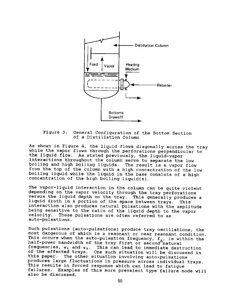
fIk_
HeatingMedium
Distillation Column
Reboiler
Figure 3 : General Configuration of the Bottom Section
of a Distillation Column
As shown in Figure 4, the liquid flows diagonally across the tray
while the vapor flows through the perforations perpendicular to
the liquid flow. As stated previously, the liquid-vapor
interactions throughout the column serve to separate the low
boiling and high boiling liquids. The result is a vapor flow
from the top of the column with a high concentration of the low
boiling liquid while the liquid in the base consists of a high
concentration of the high boiling liquid(s).
The vapor-liquid interaction in the column can be quite violent
depending on the vapor velocity through the tray perforations
versus the liquid depth on the tray. This generally produces a
liquid froth in a portion of the space between trays. This
interaction also produces natural pulsations with the amplitude
being sensitive to the ratio of the liquid depth to the vaporvelocity. These pulsations are often referred to as
auto-pulsations.
Such pulsations (auto-pulsations) produce tray oscillations, the
most dangerous of which is a resonant or near resonant condition.
This occurs when the auto-pulsation frequency, fA' is within thehalf-power bandwidth of the tray first or second natural
frequencies, _, and _2- This can lead to immediate destruction
of the affected trays. One such situation will be discussed in
this paper. The other situation involving auto-pulsations
produces large fluctuations in pressure across individual trays.
This results in forced response which can lead to fatigue
failures. Examples of this more prevalent type failure mode willalso be discussed.
90
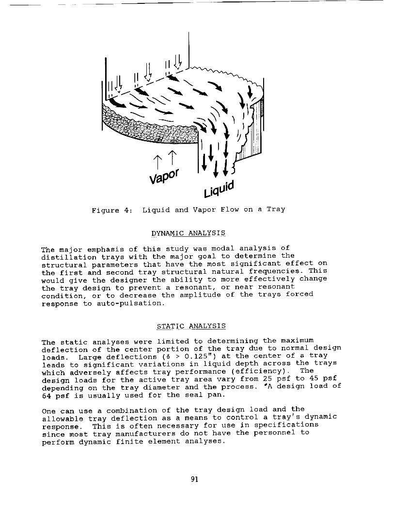
_ \'ldlIllil
biclu'u
Figure 4: Liquid and Vapor Flow on a Tray
DYNAMIC ANALYSIS
The major emphasis of this study was modal analysis of
distillation trays with the major goal to determine the
structural parameters that have the most significant effect on
the first and second tray structural natural frequencies. This
would give the designer the ability to more effectively change
the tray design to prevent a resonant, or near resonant
condition, or to decrease the amplitude of the trays forced
response to auto-pulsation.
STATIC ANALYSIS
The static analyses were limited to determining the maximum
deflection of the center portion of the tray due to normal design
loads. Large deflections (6 > 0.125") at the center of a tray
leads to significant variations in liquid depth across the trays
which adversely affects tray performance (efficiency). The
design loads for the active tray area vary from 25 psf to 45 psf
depending on the tray diameter and the process. "A design load of
64 psf is usually used for the seal pan.
One can use a combination of the tray design load and the
allowable tray deflection as a means to control a tray's dynamic
response. This is often necessary for use in specifications
since most tray manufacturers do not have the personnel to
perform dynamic finite element analyses.
91
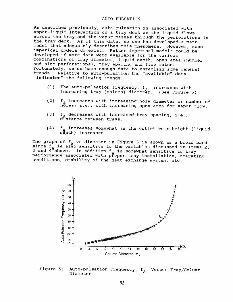
AUTO-PULSATION
As described previously, auto-pulsation is associated with
vapor-liquid interaction on a tray deck as the liquid flows
across the tray and the vapor passes through the perforations in
the tray deck. As of this date, no one has developed a math
model that adequately describes this phenomena. However, some
imperical models do exist. Better imperical models could be
developed if more data were available for the various
combinations of tray diameter, liquid depth, open area (number
and size perforations), tray spacing and flow rates.
Fortunately, we do have enough data to establish some general
trends. Relative to auto-pulsation the "available" data
"indicates" the following trends:
(1) The auto-pulsation frequency, fA' increases with
increasing tray (column) diameter. (See Figure 5)
(2) fA increases with increasing hole diameter or number ofholes; i.e., with increasing open area for vapor flow.
(3) f. decreases with increased tray spacing; i.e.
dlstance between trays.
(4) fA increases somewhat as the outlet weir height (liquiddepth) increases.
The graph of fA vs diameter in Figure 5 is shown as a broad band
since fA is also sensitive to the variables discussed in Items 2,
3 and 4 above. In addition fA is somewhat sensitive to trayperformance associated with proper tray installation, operating
conditions, stability of the heat exchange system, etc.
100
o 8o
_ zor"(D
IJ"
_ 5o
t- 40O
_ 30
_ 206
< 5
fA
SfA d
) _ I_ _
4 6 8 10 12 14 16 18 20 22!
2 24 26
Column Diameter (ft.)
Figure 5 : Auto-pulsation Frequency, fA' Versus Tray/ColumnDiameter
92
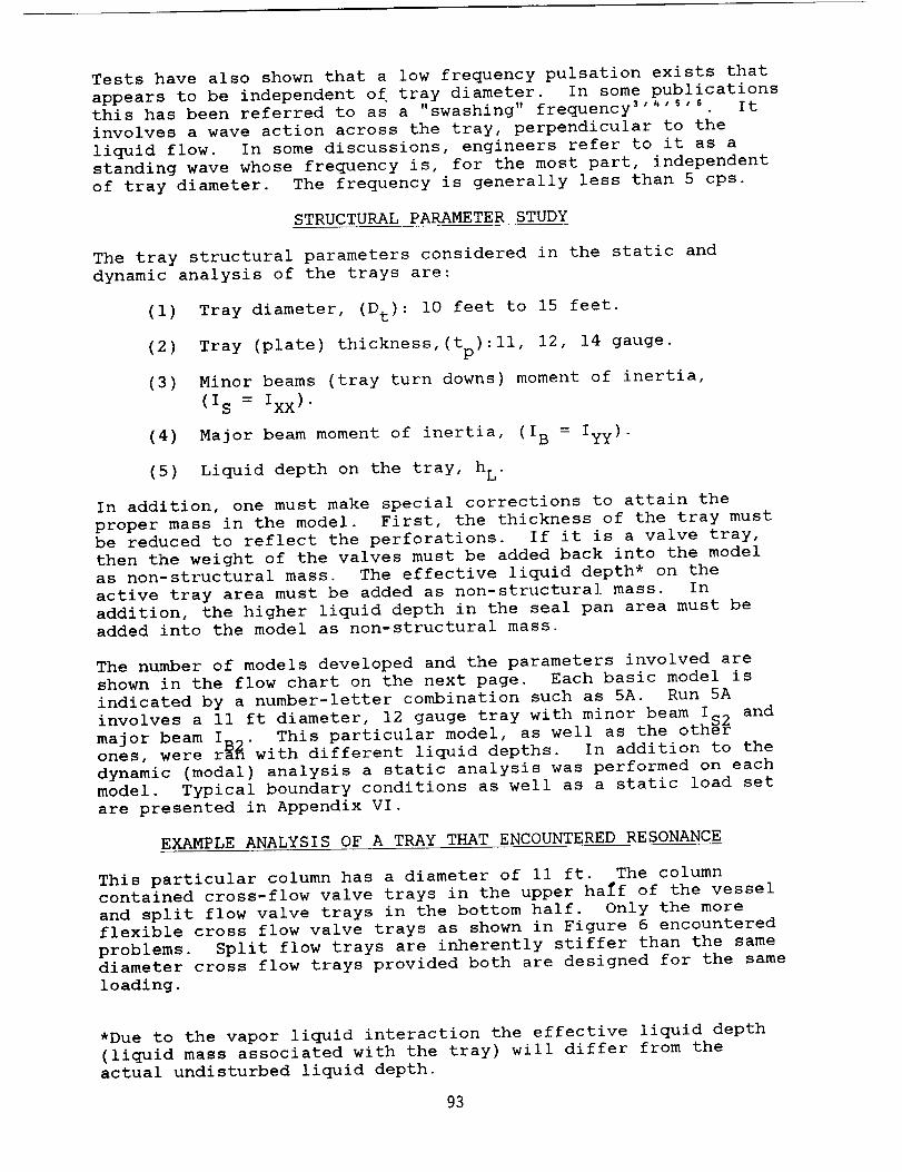
Tests have also shown that a low frequency pulsation exists that
appears to be independent of tray diameter. In some publications
this has been referred to as a "swashing" frequency ''4"_'s It
involves a wave action across the tray, perpendicular to the
liquid flow. In some discussions, engineers refer to it as a
standing wave whose frequency is, for the most part, independent
of tray diameter. The frequency is generally less than 5 cps.
STRUCTURAL PARAMETER STUDY
The tray structural parameters considered in the static and
dynamic analysis of the trays are:
(I) Tray diameter, (Dt): i0 feet to 15 feet.
(2) Tray (plate) thickness,(tp):ll, 12, 14 gauge.
(3) Minor beams (tray turn downs) moment of inertia,
(Is = Ixx).
(4) Major beam moment of inertia, (I B = Iyy).
(5) Liquid depth on the tray, h L.
In addition, one must make special corrections to attain the
proper mass in the model. First, the thickness of the tray must
be reduced to reflect the perforations. If it is a valve tray,
then the weight of the valves must be added back into the model
as non-structural mass. The effective liquid depth* on the
active tray area must be added as non-structural mass. In
addition, the higher liquid depth in the seal pan area must be
added into the model as non-structural mass.
The number of models developed and the parameters involved are
shown in the flow chart on the next page. Each basic model is
indicated by a number-letter combination such as 5A. Run 5A
involves a Ii ft diameter, 12 gauge tray with minor beam IS2 and
major beam IB2. This particular model, as well as the otherones, were ran with different liquid depths. In addition to the
dynamic (modal) analysis a static analysis was performed on each
model. Typical boundary conditions as well as a static load set
are presented in Appendix VI.
EXAMPLE ANALYSIS OF A TRAY THAT ENCOUNTERED RESONANCE
This particular column has a diameter of ii ft. The column
contained cross-flow valve trays in the upper half of the vessel
and split flow valve trays in the bottom half. Only the more
flexible cross flow valve trays as shown in Figure 6 encountered
problems. Split flow trays are inherently stiffer than the same
diameter cross flow trays provided both are designed for the same
loading.
*Due to the vapor liquid interaction the effective liquid depth
(liquid mass associated with the tray) will differ from the
actual undisturbed liquid depth.
93
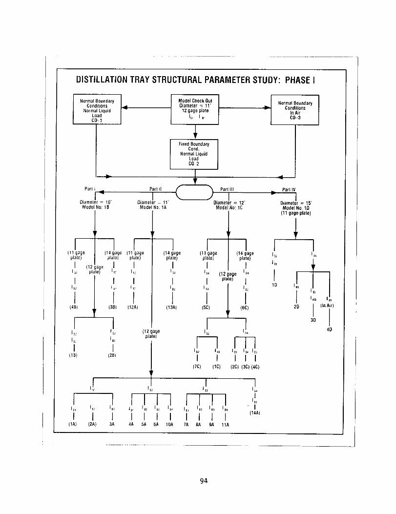
DISTILLATION TRAY STRUCTURAL PARAMETER STUDY: PHASE I
Normal Boundary I
Condilions _,Normal Liquid
LoadC0-1
Zb,==r
Parl 1'ql
Diamet!r = 10'
Model No: 1B
Part II
IOiameter = 11'
Model No: 1A
(11 gageplate)
IIs.:
II BZ
I(4B)
Ilaz
I(1B)
(12 ageplale)
r
(14 gage (11 gageplate) plate)
I I
I II Bz I _z
I I(3B) (12A)
,[
I(2B)
I !1IB' tB2 I 3 IB_
I I I I(1A) (2A) 3A 4A
_r
(12 gageplate)
,!,L,[I I
5A 6A
Model Check OutDiameter = 11'12 gage plate
Is_ I 8_
Fixed BoundaryCond.
Normal LiquidLoadC0-2
(
I(14 gage
plate)
IIs2
IIB2
I(13A)
,[-I
[7C)
Part III
Diameb = 12'Mode No: 1C
_r
(11 gage (14 gageplate) plate)
I IIs4 (12 gage Is_
[ plate) I
I B3 I B3
I I(sc) (6c)
Ir
I !2 I !4
I I I I(1C) (2C) (3C)(4C)
IIOA
II
7A
,L,[,[8A 9A 11A
I Normal Boundary
ConditionsIn AirC0-3
Part IVI
Diameter = 15'Model No. 1D
(11 gage plate)
I II s_ I s4
1_2 I!I !ID I_
I IMs
3D
(In Air)
I4D
94
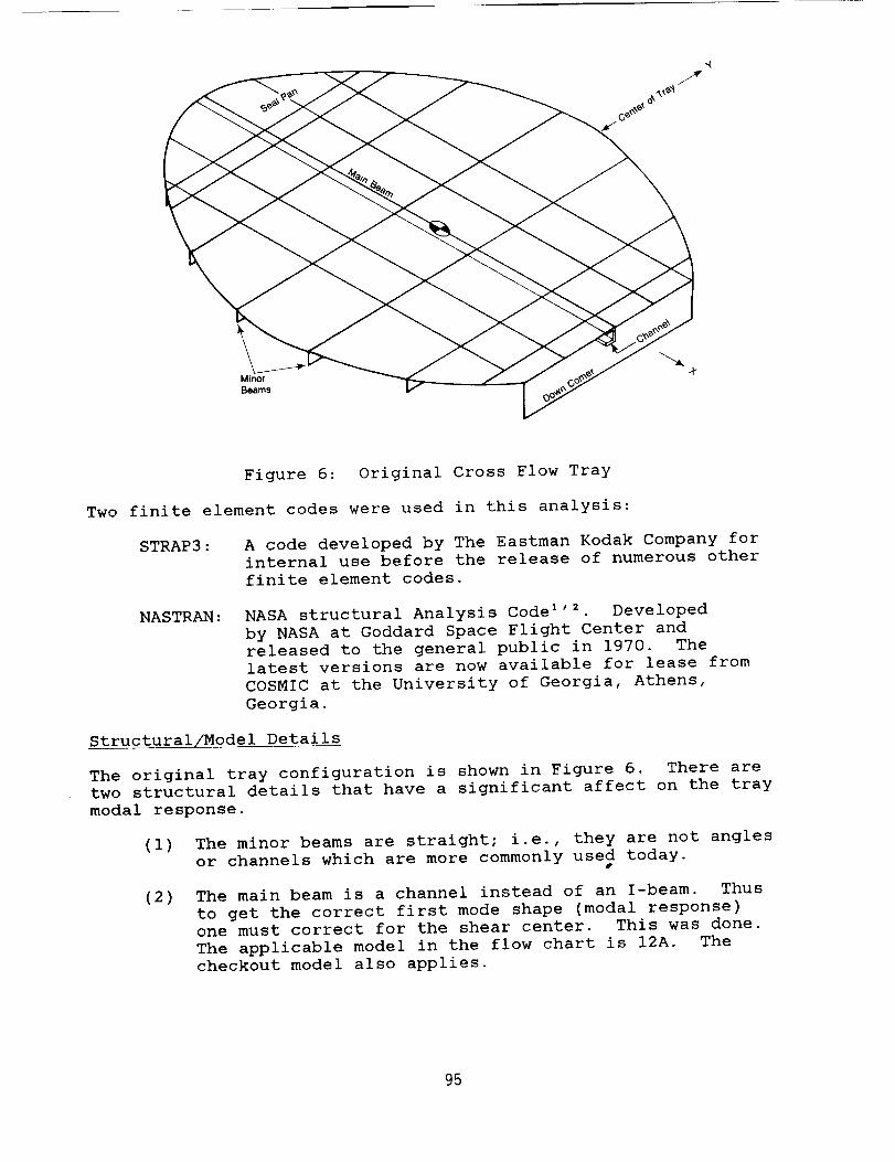
Minor
Beams
Figure 6: Original Cross Flow Tray
Two finite element codes were used in this analysis:
STRAP3: A code developed by The Eastman Kodak Company forinternal use before the release of numerous other
finite element codes.
NASTRAN: NASA structural Analysis Code *'2 Developed
by NASA at Goddard Space Flight Center and
released to the general public in 1970. The
latest versions are now available for lease from
COSMIC at the University of Georgia, Athens,
Georgia.
Structural/Model Details
The original tray configuration is shown in Figure 6. There are
two structural details that have a significant affect on the tray
modal response.
(1)
(2)
The minor beams are straight; i.e., they are not angles
or channels which are more commonly used today.B
The main beam is a channel instead of an I-beam. Thus
to get the correct first mode shape (modal response)
one must correct for the shear center. This was done.
The applicable model in the flow chart is 12A. The
checkout model also applies.
95
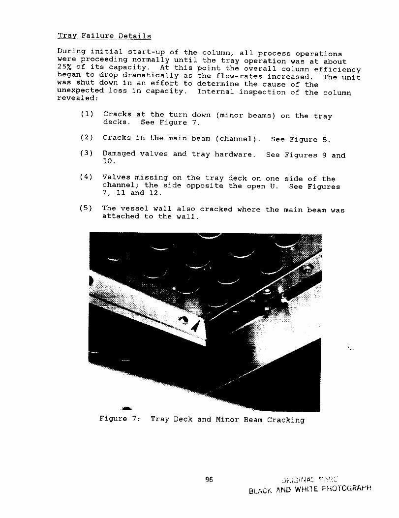
Tray Failure Details
During initial start-up of the column, all process operations
were proceeding normally until the tray operation was at about
25_ of its capacity. At this point the overall column efficiency
began to drop dramatically as the flow-rates increased. The unitwas shut down in an effort to determine the cause of the
unexpected loss in capacity. Internal inspection of the columnrevealed:
(1) Cracks at the turn down (minor beams) on the tray
decks. See Figure 7.
(2) Cracks in the main beam (channel). See Figure 8.
(3) Damaged valves and tray hardware.
I0.
See Figures 9 and
(4) Valves missing on the tray deck on one side of the
channel; the side opposite the open U. See Figures
7, II and 12.
(5) The vessel wall also cracked where the main beam was
attached to the wall.
Figure 7 : Tray Deck and Minor Beam Cracking
%.
96
BL/-kCK_ Arid WHILE PHOTO C-RAFt}!
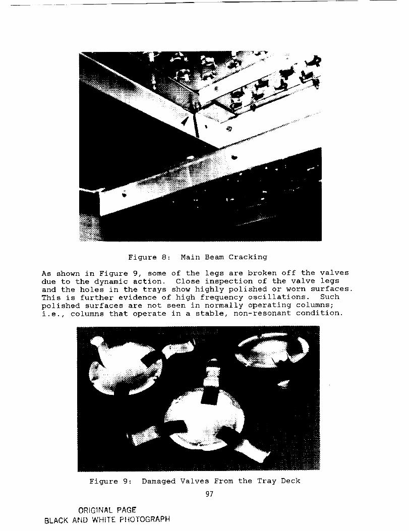
Figure 8: Main Beam Cracking
As shown in Figure 9, some of the legs are broken off the valvesdue to the dynamic action. Close inspection of the valve legsand the holes in the trays show highly polished or worn surfaces.This is further evidence of high frequency oscillations. Suchpolished surfaces are not seen in normally operating columns;i.e., columns that operate in a stable, non-resonant condition.
Figure 9: Damaged Valves From the Tray Deck
97
ORIGINAl PAGE
BLACK AND WHITE PHOTOGRAPH
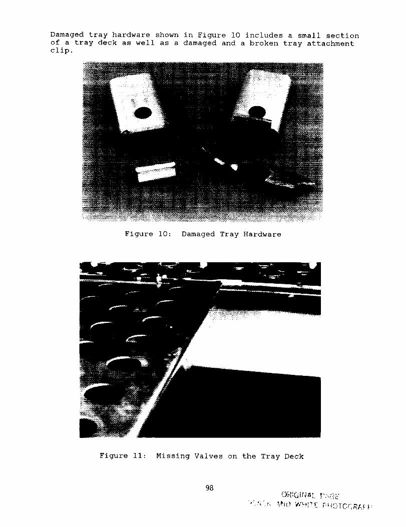
Damaged tray hardware shown in Figure i0 includes a small section
of a tray deck as well as a damaged and a broken tray attachment
clip.
Figure i0: Damaged Tray Hardware
Figure Ii: Missing Valves on the Tray Deck
98
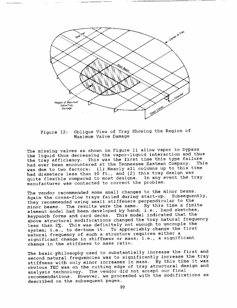
Region of MaximumValve/Tray
Damage
Figure 12: Oblique View of Tray Showing the Region of
Maximum Valve Damage
The missing valves as shown in Figure II allow vapor to bypass
the liquid thus decreasing the vapor-liquid interaction and thus
the tray efficiency. This was the first time this type failure
had ever been encountered at the Tennessee Eastman Company. This
was due to two factors: (I) Nearly all columns up to this time
had diameters less than I0 ft., and (2) this tray design was
quite flexible compared to most designs. In any event the tray
manufacturer was contacted to correct the problem.
The vendor recommended some small changes to the minor beams.
Again the cross-flow trays failed during start-up. Subsequently,
they recommended using small stiffeners perpendicular to the
minor beams. The results were the same. By this time a finite
element model had been developed by hand; i.e., hand sketches,
keypunch forms and card decks. This model indicated that the
above structural modifications changed the tray natural frequency
less than 2_. This was definitely not enough to uncouple the
system; i.e., to de-tune it. To appreciably change the first
natural frequency of such a structure requires either a
significant change in stiffness or mass; i.e., a significant
change in the stiffness to mass ratio.
The basic philosophy used to substantially increase the first and
second natural frequencies was to significantly increase the tray
stiffness with only minor increases in mass. By this time it was
obvious TEC was on the cutting edge of tray structural design and
analysis technology. The vendor did not accept our final
recommendations. However, we proceeded with the modifications as
described on the subsequent pages.
99
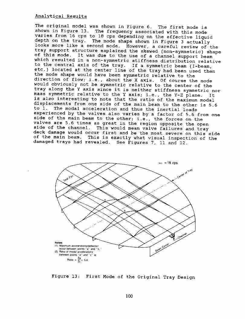
Analytical Results
The original model was shown in Figure 6. The first mode is
shown in Figure 13. The frequency associated with this mode
varies from 16 cps to 18 cps depending on the effective liquid
depth on the tray. The mode shape shown in Figure 3 actually
looks more like a second mode. However, a careful review of the
tray support structure explained the skewed (non-symmetric) shape
of this mode. It was due to the use of a channel support beam
which resulted in a non-symmetric stiffness distribution relative
to the central axis of the tray. If a symmetric beam (I-beam,
etc.) located at the center line of the tray had been used then
the mode shape would have been symmetric relative to the
direction of flow; i.e., about the X axis. Of course the mode
would obviously not be symmetric relative to the center of the
tray along the Y axis since it is neither stiffness symmetric nor
mass symmetric relative to the Y axis; i.e., the Y-Z plane. It
is also interesting to note that the ratio of the maximum modal
displacements from one side of the main beam to the other is 5.6to I. The modal acceleration and thus the inertial loads
experienced by the valves also varies by a factor of 5.6 from one
side of the main beam to the other; i.e., the forces on the
valves are 5.6 times as great in the region opposite the open
side of the channel. This would mean valve failures and tray
deck damage would occur first and be the most severe on this side
of the main beam. This is exactly what visual inspection of the
damaged trays had revealed. See Figures 7, II and 12.
_1 =18 cps
Notes:
(1) Maximum accelerations/deflectionoccur between points "a" and "b."
(2) Ratio of modal accelerationsbetween points "a" and "c" is:
zaRatio = Zc = 5_6
Figure 13: First Mode of the Original Tray Design
100
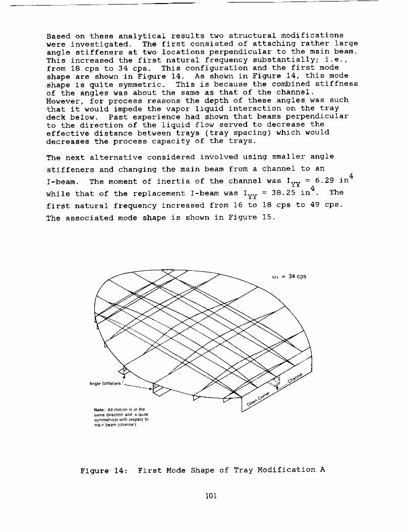
Based on these analytical results two structural modifications
were investigated. The first consisted of attaching rather large
angle stiffeners at two locations perpendicular to the main beam.
This increased the first natural frequency substantially; i.e.,
from 18 cps to 34 cps. This configuration and the first mode
shape are shown in Figure 14. As shown in Figure 14, this mode
shape is quite symmetric. This is because the combined stiffness
of the angles was about the same as that of the channel.
However, for process reasons the depth of these angles was such
that it would impede the vapor liquid interaction on the tray
deck below. Past experience had shown that beams perpendicular
to the direction of the liquid flow served to decrease the
effective distance between trays (tray spacing) which would
decreases the process capacity of the trays.
The next alternative considered involved using smaller angle
stiffeners and changing the main beam from a channel to an4
I-beam. The moment of inertia of the channel was Iyy = 6.29 in4
while that of the replacement I-beam was Iyy = 38.25 in The
first natural frequency increased from 16 to 18 cps to 49 cps.
The associated mode shape is shown in Figure 15.
Angle Stiffeners
Note: All motion is in the
same direction end is quite
symmetrical with respect to
main beam (channel).
Figure 14: First Mode Shape of Tray Modification A
i01
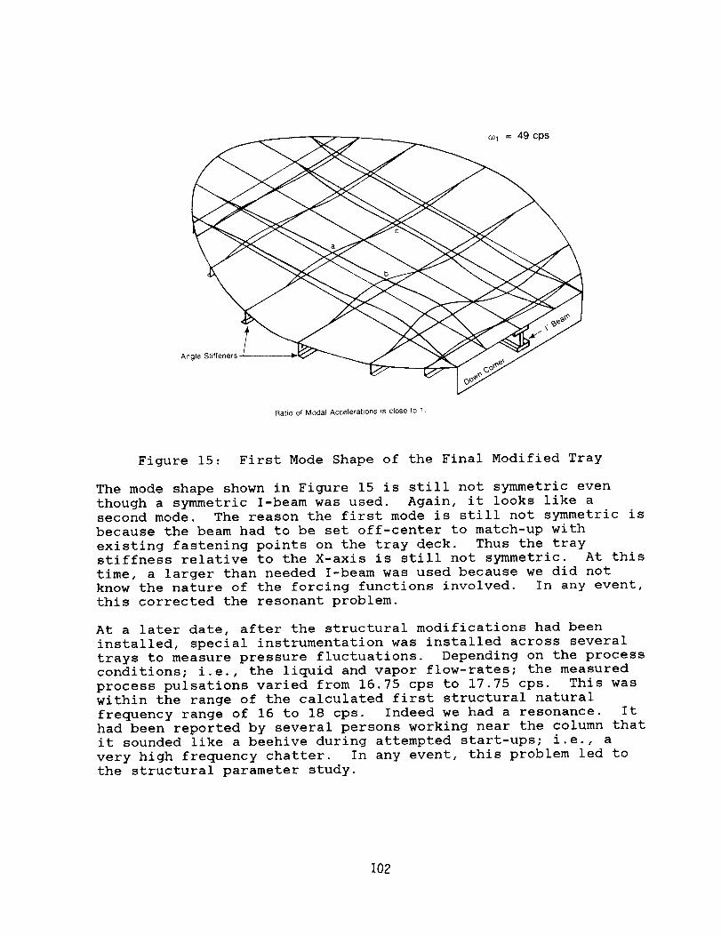
_t = 49 cps
Angle Stiffeners I
Ratio of Modal Acceleralions is close to 1,
Figure 15: First Mode Shape of the Final Modified Tray
The mode shape shown in Figure 15 is still not symmetric even
though a symmetric I-beam was used. Again, it looks like a
second mode. The reason the first mode is still not symmetric is
because the beam had to be set off-center to match-up with
existing fastening points on the tray deck. Thus the traystiffness relative to the X-axis is still not symmetric. At this
time, a larger than needed I-beam was used because we did not
know the nature of the forcing functions involved. In any event,
this corrected the resonant problem.
At a later date, after the structural modifications had been
installed, special instrumentation was installed across several
trays to measure pressure fluctuations. Depending on the process
conditions; i.e., the liquid and vapor flow-rates; the measured
process pulsations varied from 16.75 cps to 17.75 cps. This was
within the range of the calculated first structural natural
frequency range of 16 to 18 cps. Indeed we had a resonance. It
had been reported by several persons working near the column that
it sounded like a beehive during attempted start-ups; i.e., a
very high frequency chatter. In any event, this problem led to
the structural parameter study.
102
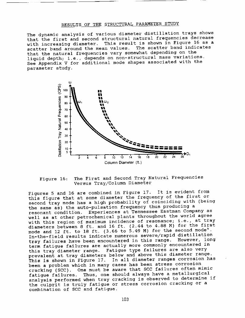
RESULTS OF THE STRUCTURAL PARAMETER STUDY
The dynamic analysis of various diameter distillation trays shows
that the first and second structural natural frequencies decrease
with increasing diameter. This result is shown in Figure 16 as a
scatter band around the mean values. The scatter band indicates
that the natural frequencies vary somewhat depending on the
liquid depth; i.e., depends on non-structural mass variations.
See Appendix V for additional mode shapes associated with the
parameter study.
60
.,
,ot\\ v,00f \\ %
\\ "-'-
30 %%
_5 5 D,2 4 6 8 10 12 14 16 18 20 22 24 26
Column Diameter (ft.)
Figure 16 : The First and Second Tray Natural Frequencies
Versus Tray/Column Diameter
Figures 5 and 16 are combined in Figure 17. It is evident from
this figure that at some diameter the frequency of the first or
second tray mode has a high probability of coinciding with (being
the same as) the auto-pulsation frequency thus producing a
resonant condition. Experiences at Tennessee Eastman Company as
well as at other petrochemical plants throughout the world agree
with this region of maximum incidence of resonance; i.e., at tray
diameters between 8 ft. and 16 ft. (2.44 to 4.88 M) for the first
mode and 12 ft. to 18 ft. (3.66 to 5.49 M) for the second mode _.
In-the-field results indicate numerous severe/rapid distillation
tray failures have been encountered in this range. However, long
term fatigue failures are actually more commonly encountered in
this tray diameter range. Fatigue type failures are also very
prevalent at tray diameters below and above this diameter range.
This is shown in Figure 17. In all diameter ranges corrosion has
been a problem which in many cases has been stress corrosion
cracking (SCC). One must be aware that SCC failures often mimic
fatigue failures. Thus, one should always have a metallurgical
analysis performed when tray cracking is observed to determine if
the culprit is truly fatigue or stress corrosion cracking or a
combination of SCC and fatigue.
103
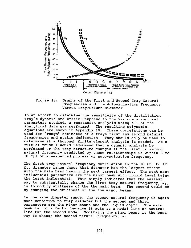
100 I_ _i _.._
I II II
u._ 50 f
_o 20 _=_< 10 ==, ,m ...= _==_
5 __ _ ==' ="' == _ ="= Dt
2 4 6 8 10 12 14 16 18 20 22 24 26Fatiguedue to J Resonar,ce or Fatigue I Fatiguedue to ForcedResponse
ForcedResponse I due to Forced Response I or Possible Resonance withr.- -'1 Individual Panels.
Column Diameter (ft.)
Figure 17 : Graphs of the First and Second Tray Natural
Frequencies and the Auto-Pulsation Fre_lency
Versus Tray/Column Diameter
In an effort to determine the sensitivity of the distillation
tray's dynamic and static response to the various structural
parameters studied, a regression analysis using all of the
analytical data was performed. The resulting polynomial
equations are shown in Appendix IV. These correlations can be
used for "rough" estimates of a trays first and second natural
frequencies and static deflection. They should only be used to
determine if a thorough finite element analysis is needed. As a
rule of thumb I would recommend that a dynamic analysis be
performed or the tray structure changed if the first or second
natural frequency predicted by these relationships is within 8 to
I0 cps of a suspected process or auto-pulsation frequency.
The first tray natural frequency correlation in the I0 ft. to 12
ft. diameter range shows that diameter has the largest effect
with the main beam having the next largest effect. The next most
influential parameters are the minor beam with liquid level being
the least influential. This simply indicates that the easiest
way to substantially change the first tray natural frequency, w,,
is to modify stiffness of the the main beam. The second would be
by changing the stiffness of the the minor beams.
In the same diameter range, the second natural frequency is again
most sensitive to tray diameter but the second and third
parameters are the minor beams and the liquid depth. The mainbeam is not a factor because it acts as a nodal line or neutral
line for the second mode. Modifying the minor beams is the best
way to change the second natural frequency, w_.
104
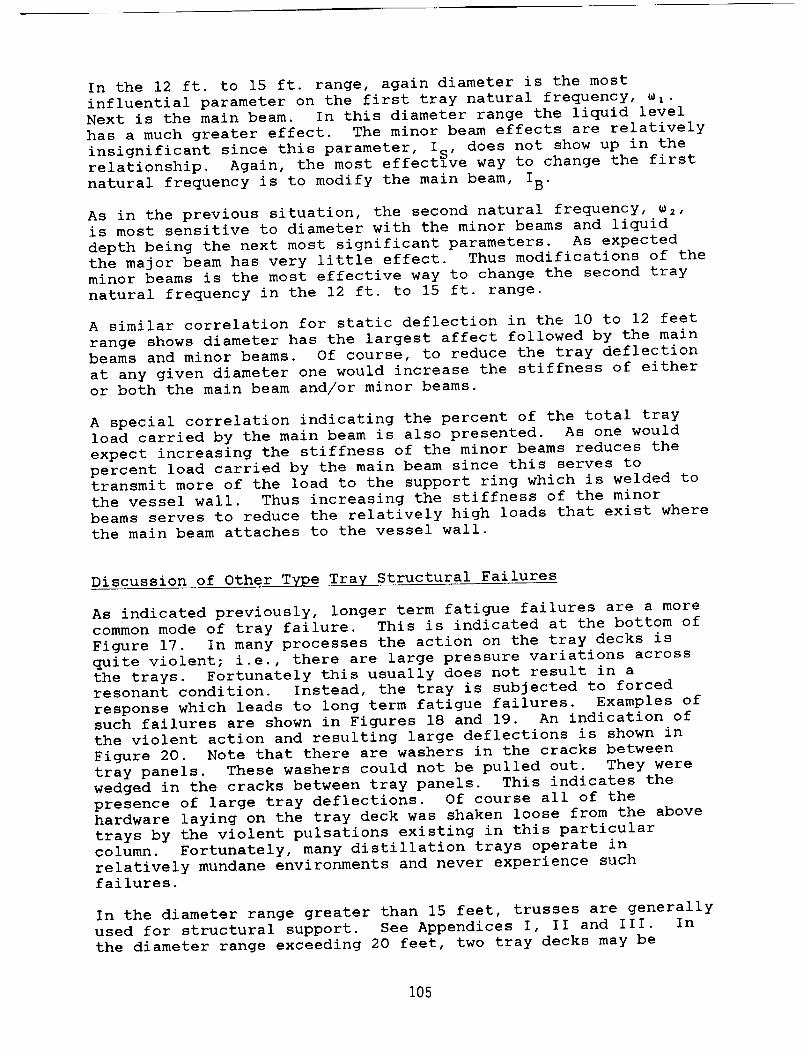
In the 12 ft. to 15 ft. range, again diameter is the most
influential parameter on the first tray natural frequency, w,.
Next is the main beam. In this diameter range the liquid level
has a much greater effect. The minor beam effects are relatively
insignificant since this parameter, I_, does not show up in the
relationship. Again, the most effectlve way to change the first
natural frequency is to modify the main beam, IB.
As in the previous situation, the second natural frequency, _2,
is most sensitive to diameter with the minor beams and liquid
depth being the next most significant parameters. As expected
the major beam has very little effect. Thus modifications of the
minor beams is the most effective way to change the second tray
natural frequency in the 12 ft. to 15 ft. range.
A similar correlation for static deflection in the i0 to 12 feet
range shows diameter has the largest affect followed by the main
beams and minor beams. Of course, to reduce the tray deflection
at any given diameter one would increase the stiffness of either
or both the main beam and/or minor beams.
A special correlation indicating the percent of the total tray
load carried by the main beam is also presented. As one would
expect increasing the stiffness of the minor beams reduces the
percent load carried by the main beam since this serves to
transmit more of the load to the support ring which is welded to
the vessel wall. Thus increasing the stiffness of the minor
beams serves to reduce the relatively high loads that exist where
the main beam attaches to the vessel wall.
Discussion of Other Type Tray Structural Failures
As indicated previously, longer term fatigue failures are a more
common mode of tray failure. This is indicated at the bottom of
Figure 17. In many processes the action on the tray decks is
quite violent; i.e., there are large pressure variations across
the trays. Fortunately this usually does not result in a
resonant condition. Instead, the tray is subjected to forced
response which leads to long term fatigue failures. Examples of
such failures are shown in Figures 18 and 19. An indication of
the violent action and resulting large deflections is shown in
Figure 20. Note that there are washers in the cracks between
tray panels. These washers could not be pulled out. They were
wedged in the cracks between tray panels. This indicates the
presence of large tray deflections. Of course all of the
hardware laying on the tray deck was shaken loose from the above
trays by the violent pulsations existing in this particular
column. Fortunately, many distillation trays operate in
relatively mundane environments and never experience suchfailures.
In the diameter range greater than 15 feet, trusses are generally
used for structural support. See Appendices I, II and III. In
the diameter range exceeding 20 feet, two tray decks may be
105
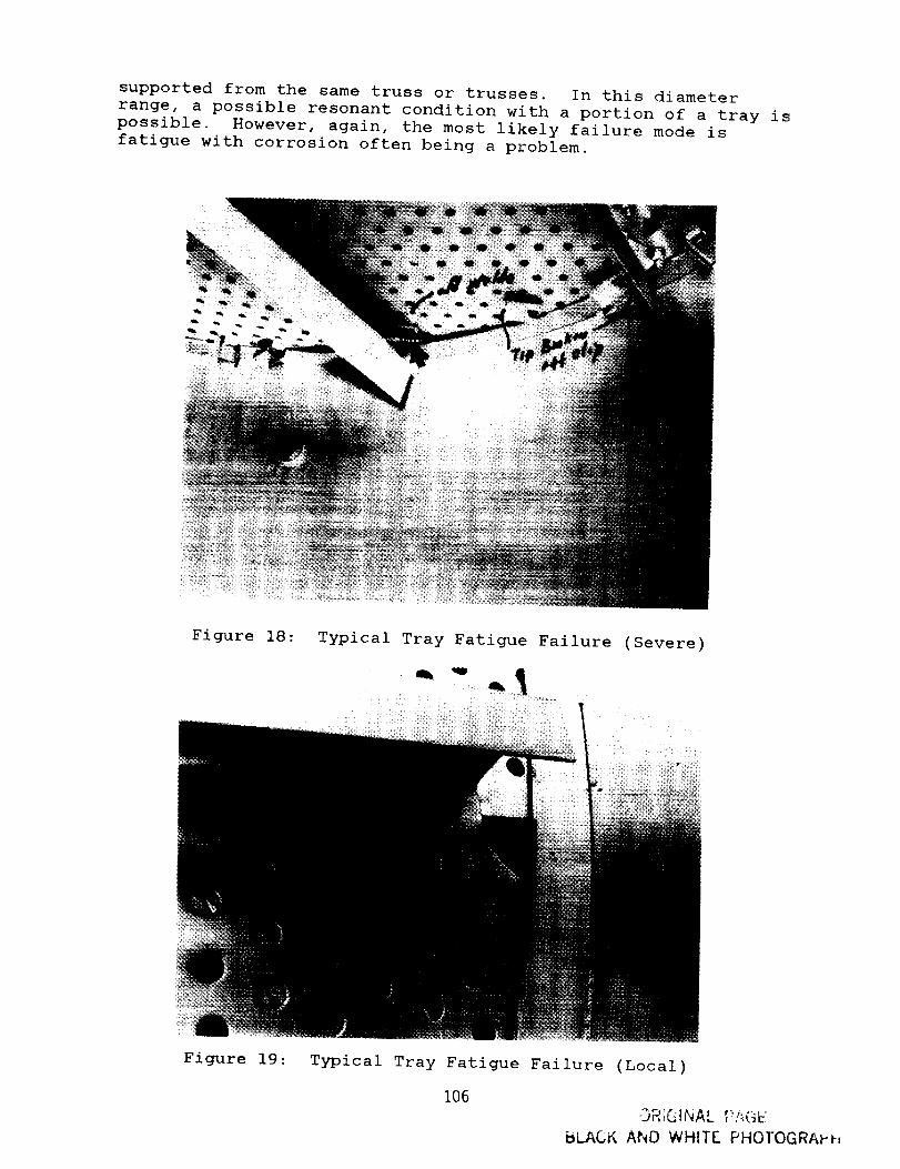
supported from the same truss or trusses. In this diameter
range, a possible resonant condition with a portion of a tray is
possible. However, again, the most likely failure mode is
fatigue with corrosion often being a problem.
Figure 18: Typical Tray Fatigue Failure (Severe)
Figure 19: Typical Tray Fatigue Failure (Local)
106
.,jH_GINA,.. ;'_'_(:i _::
BLACK AND WHITE PHOTOGRAt-'t-_
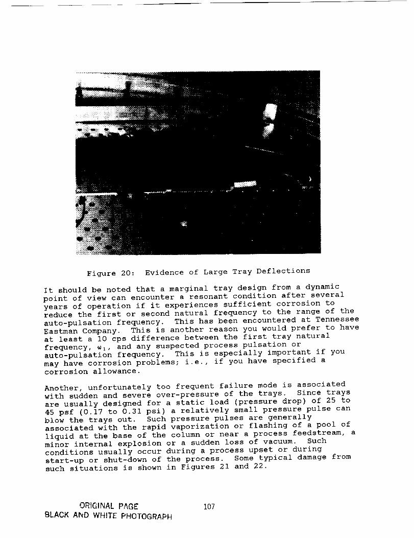
Figure 20: Evidence of Large Tray Deflections
It should be noted that a marginal tray design from a dynamic
point of view can encounter a resonant condition after several
years of operation if it experiences sufficient corrosion to
reduce the first or second natural frequency to the range of the
auto-pulsation frequency. This has been encountered at Tennessee
Eastman Company. This is another reason you would prefer to have
at least a I0 cps difference between the first tray natural
frequency, _i, and any suspected process pulsation or
auto-pulsation frequency. This is especially important if you
may have corrosion problems; i.e., if you have specified a
corrosion allowance.
Another, unfortunately too frequent failure mode is associated
with sudden and severe over-pressure of the trays. Since trays
are usually designed for a static load (pressure drop) of 25 to
45 psf (0.17 to 0.31 psi) a relatively small pressure pulse can
blow the trays out. Such pressure pulses are generally
associated with the rapid vaporization or flashing of a pool of
liquid at the base of the column or near a process feedstream, a
minor internal explosion or a sudden loss of vacuum. Such
conditions usually occur during a process upset or during
start-up or shut-down of the process. Some typical damage from
such situations is shown in Figures 21 and 22.
ORIGINAL PAGE
BLACK AND WHITE PHOTOGRAPH107
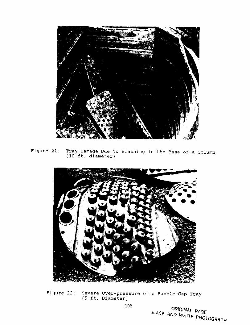
Figure 21: Tray Damage Due to Flashing in the Base of a Column
(I0 ft. diameter)
Figure 22 : Severe Over-pressure of a Bubble-Cap Tray
(5 ft. Diameter)
108
ORIGINAL PA_E
JLACK AND WHtTE PHOToGRApN
Certain sections of a column are more susceptible to such damage
than others. As a result we generally increase the design load
for the trays in these regions; i.e., use a design load of 90 to
130 psf. It is important to realize that the tray panels are
designed such that they will come apart when subjected to a large
over pressure; i.e., they serve as a pressure relief mechanism.
If this was not done, then the over pressure would have to be
absorbed by the vessel wall. This would in many cases rip a hole
in the vessel wall. To prevent such occurrences would require
much thicker vessel walls along with special reenforcements where
main beams are attached to the vessel. This would substantially
increase the cost of such units and adversely affect product
costs. It should also be realized that the tray panels, as
designed, are quite flexible and can easily be repositioned. For
instance, the seemingly severe damage shown in Figure 21 was
repaired within a few weeks; i.e., the trays were reassembled
with very few new parts being required.
Conclusions:
This structural parameter study has shown that cross flow
distillation trays in the I0 to 15 feet diameter range are
susceptible to resonant conditions. It has further identified
which structural parameters can be most effectively used to
correct a resonant condition and reduce fatigue damage. In
addition, these results can be used to prepare static design
specifications that reflect dynamic requirements. This is
important since many distillation tray vendors at this time do
not have the capability to perform the dynamic analysis and thus
cannot comply with dynamic specifications.
A future study, Phase If, will extend this cross flow
distillation tray structural parameter study to a diameter rangeof 3 feet to I0 feet.
109
(1)
(2)
(3)
(4)
(s)
(6)
REFERENCES
NASTRAN Users Manual (NASA SP-222), COSMIC, Barrows Hall,
University of Georgia, Athens, Georgia 30601
NASTRAN Programmers Manual (NASA SP-223), COSMIC, Barrows
Hall, University of Georgia, Athens, Georgia 30601
Priestman, G. H.; Brown, D. J.: "The Mechanism of Pressure
Pulsations in Sieve Tray Columns", Institute of Chemical
Engineers, Dept. of Chemical Engineering & Fuel Technology,
Sheffield University, England, Trans I ChemE, Vol. 59, 1981.
Priestman, G.H.; Brown, D. J.; Kohler, H. K.; "Pressure
Pulsations In Sieve-Tray Columns", ICHEM.E. Symposium SeriesNo. 56.
Biddulph, M. W.; Stephens, D. J.; "Oscillating Behavior on
Distillation Trays," Dept. of Chemical Engineering,
University of Nottingham, University Park, England.
Brierley, RJP; Whyman, PJM; Erskine, JB; "Flow Induced
Vibration of Distillation and Absorption Column Trays",
Imperial Chemical Industries Limited, I. Chem. E. Symposium,Series No. 56.
II
III
IV
V
VI
LIST OF APPENDICES
Typical Valve Trays
Typical Sieve Trays
Large Diameter Trays and Other Tray Configurations
Regression Analysis of Analytical Results
Some Typical Mode Shapes
Typical Boundary Conditions and an Example Static Load Set
11o
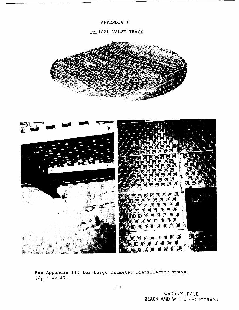
APPENDIX I
TYPICAL VALVE TRAYS
See Appendix Ill for Large Diameter Distillation Trays(D t > 16 ft.)
111
ORIGINAL FAGE
BLACK AND WHITE PHOTOGRAPH
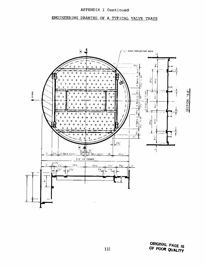
APPENDIX I Continued
ENGINEERING DRAWING OF A TYPICAL VALVE TRAYS
112
ORIGINAL PAGE IS
OF POOR QUALITY
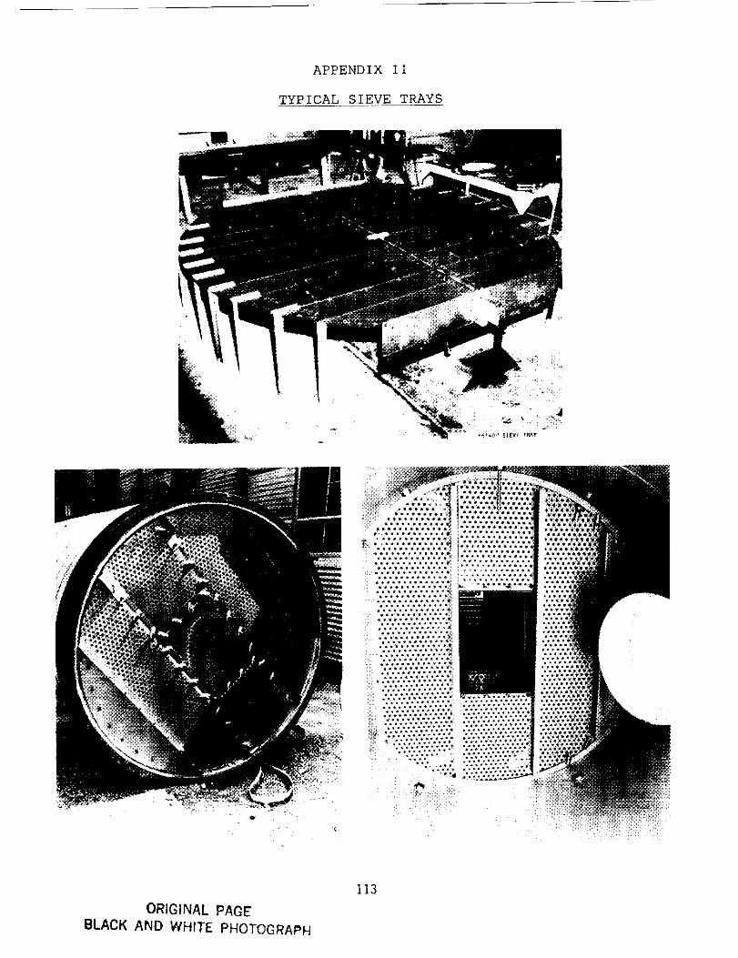
APPENDIX II
TYPICAL SIEVE TRAYS
BLACKORIGINAL
AND WHITEPAGE'
PHOTOGRAPH
113
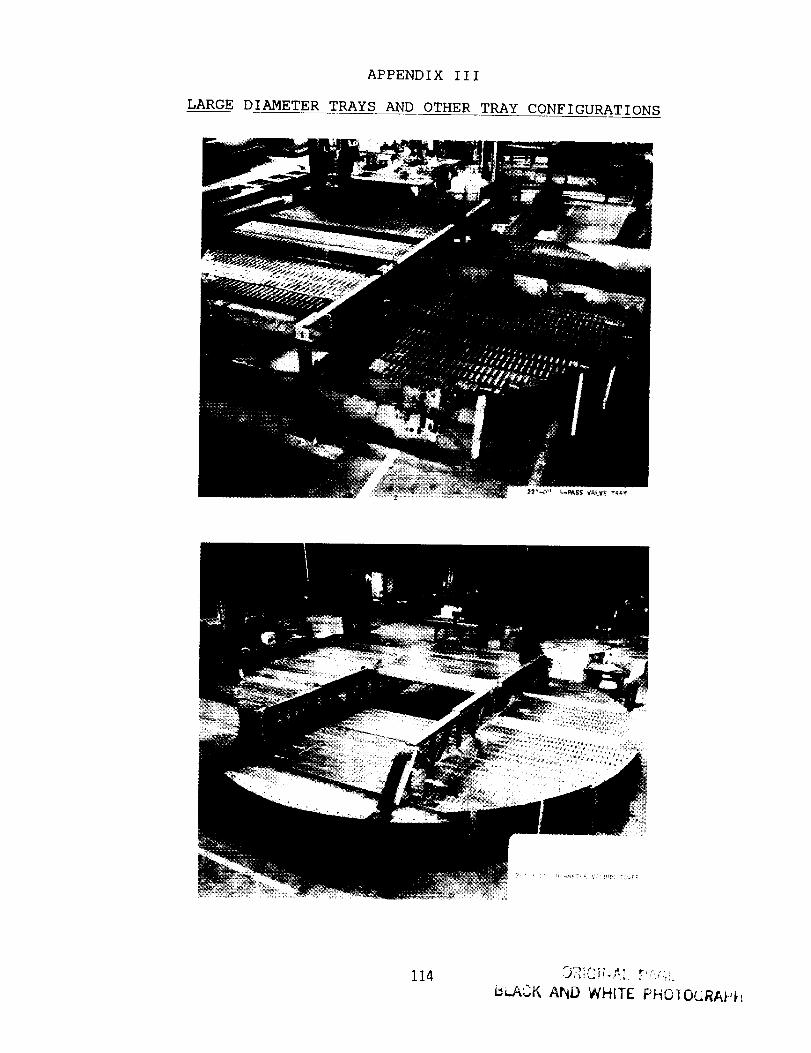
APPENDIX III
LARGE DIAMETER TRAYS AND OTHER TRAY CONFIGURATIONS
114
_LACK AIND WHITE PHOIO&RAPI, i
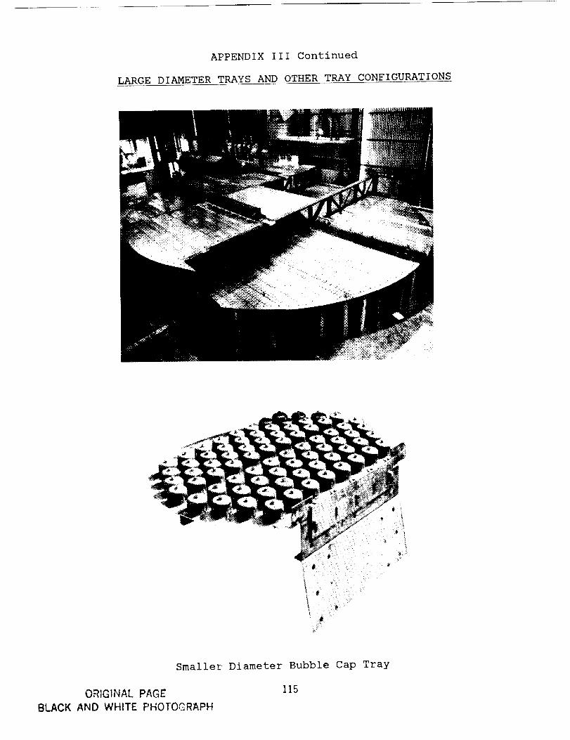
APPENDIX III Continued
LARGE DIAMETER TRAYS AND OTHER TRAY CONFIGURATIONS
#
!.1
Smaller Diameter Bubble Cap Tray
OR]GINAL PAGE 115
BLACK AND WHITE PHOTOGRAPH
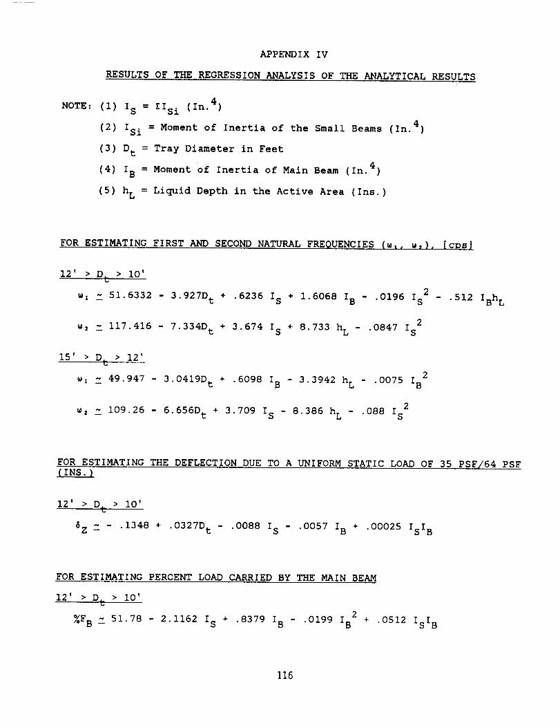
APPENDIX IV
RESULTS OF THE REGRESSION ANALYSIS OF THE ANALYTICAL RESULTS
NOTE: (I) Is = EISi (In. 4)
(2) ISi = Moment of Inertia of the Small Beams (In.
(3) D t = Tray Diameter in Feet
(4) IB = Moment Of Inertia of Main Beam (In. 4)
(5) h L = Liquid Depth in the Active Area (Ins.)
4)
FOR ESTIMATING FIRST AND SECOND NATURAL FREQUENCIES (w,, w,), [cps]
12' > D t > 10'
w, ~ 51.6332 - 3.927D t + .6236 Is + 1.6068 IB - .0196 I2
- .512S
2w, ~ 117.416 - 7.334D t + 3.674 Is + 8.733 h L - .0847 Is
15' > D t > 12'
wl C 49.947 - 3.0419D t + .6098 IB - 3.3942 h L - .0075 IB2
2w, ~ 109.26 - 6.656D t + 3.709 IS - 8.386 h L - .088 IS
IBh L
FOR ESTIMATING THE DEFLECTION DUE TO A UNIFORM STATIC LOAD OF 35 PSF/64 PSF(INS.)
12' > D t > I0'
6z ~ - .1348 + .0327D t - .0088 IS - .0057 IB + .00025 ISl B
FOR ESTIMATING PERCENT LOAD CARRIED BY THE MAIN BEAM
12' > D t > I0'
2%F B ~ 51.78 - 2.1162 Is + .8379 IB - .0199 IB + .0512 I I
S B
116
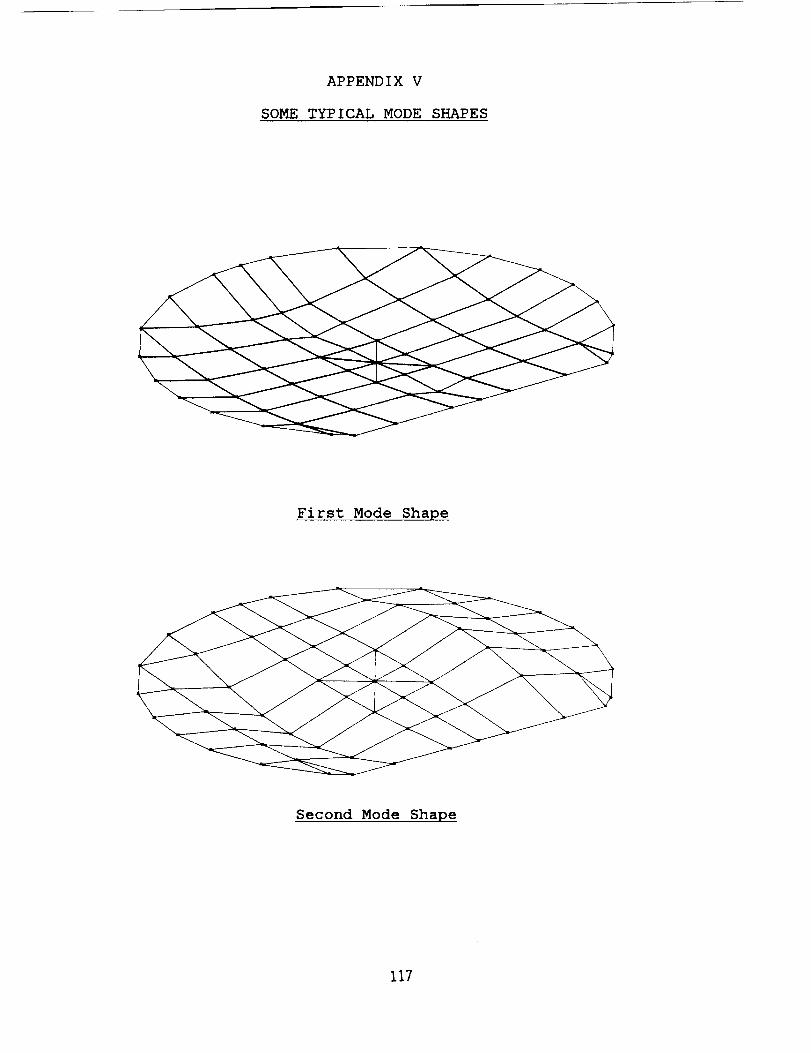
APPENDIX V
SOME TYPICAL MODE SHAPES
First Mode Shape
Second Mode Shape
117
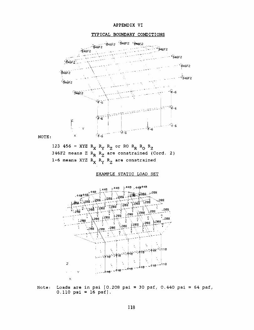
NOTE:
APPENDIX Vl
TYPICAL BOUNDARY CONDITIONS
_4_F2
_ - _ ..... -_ t_46F 2
_-'_46F2
"_-d 'l
..... #4_¥__
123 456 = XYZ R x Ry R Z or RO RR RO R Z
346F2 means Z R R R Z are constrained (Cord. 2)
1-6 means XYZ R X Ry R Z are constrained
EXAMPLE STATIC LOAD SET
288
.208
Note:
iI ,
/
Loads are in psi [0.208 psi = 30 psf, 0.440 psi = 64 psf,
0.II0 psi = 16 psf].
118
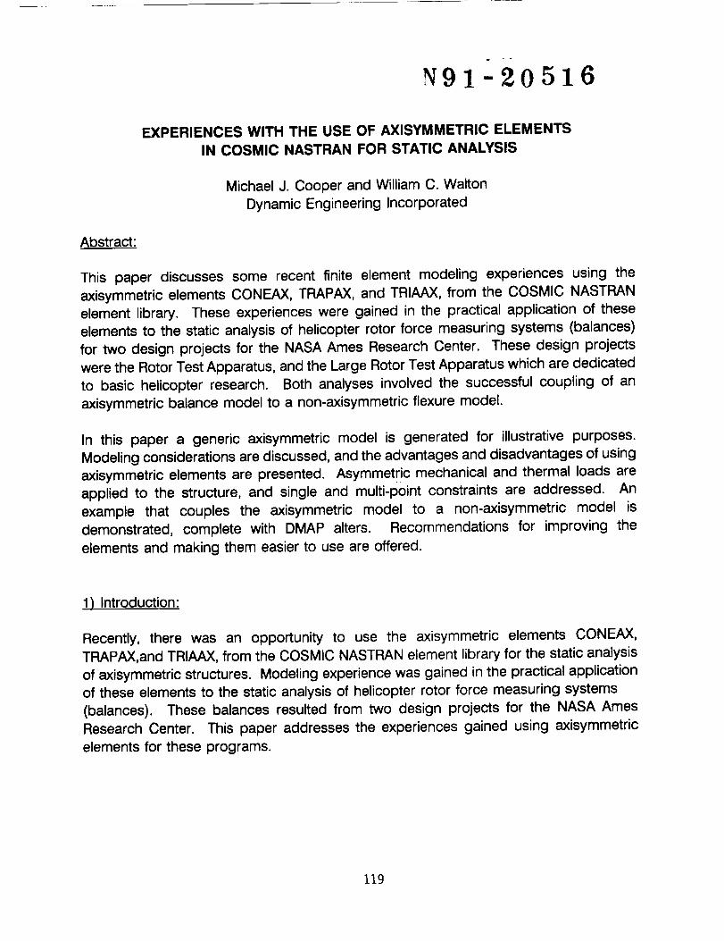
N91-20516
EXPERIENCES WITH THE USE OF AXISYMMETRIC ELEMENTS
IN COSMIC NASTRAN FOR STATIC ANALYSIS
Abstract:
Michael J. Cooper and William C. Walton
Dynamic Engineering Incorporated
This paper discusses some recent finite element modeling experiences using the
axisymmetric elements CONEAX, TRAPAX, and TRIAAX, from the COSMIC NASTRAN
element library. These experiences were gained in the practical application of these
elements to the static analysis of helicopter rotor force measuring systems (balances)
for two design projects for the NASA Ames Research Center. These design projects
were the Rotor Test Apparatus, and the Large Rotor Test Apparatus which are dedicated
to basic helicopter research. Both analyses involved the successful coupling of an
axisymmetric balance model to a non-axisymmetric flexure model.
In this paper a generic axisymmetric model is generated for illustrative purposes.
Modeling considerations are discussed, and the advantages and disadvantages of using
axisymmetric elements are presented. Asymmetric mechanical and thermal loads are
applied to the structure, and single and multi-point constraints are addressed. An
example that couples the axisymmetric model to a non-axisymmetric model is
demonstrated, complete with DMAP alters. Recommendations for improving the
elements and making them easier to use are offered.
1) Introduction:
Recently, there was an opportunity to use the axisymmetric elements CONEAX,
TRAPAX,and TRIAAX, from the COSMIC NASTRAN element library for the static analysis
of axisymmetric structures. Modeling experience was gained in the practical application
of these elements to the static analysis of helicopter rotor force measuring systems
(balances). These balances resulted from two design projects for the NASA Ames
Research Center. This paper addresses the experiences gained using axisymmetric
elements for these programs.
119

Two large dynamic rotor force measurement systems were designed as part of the RotorTest Apparatus (RTA) and Large Rotor Test Apparatus (LRTA) programs. All the force
generated by the rotor blades passes through four flexure bars that constitute the critical
portion of the balance. These flexures rest on a very large axisymmetric base piece and
are surmounted by a relatively large axisymmetric ring and axisymmetric mast. Thus,the structure is extensively axisymmetric with a relatively small portion which is notaxisymmetric.
The flexures must satisfy strength, sensitivity, fatigue, and frequency constraints. The
constraints are severe and contradictory. For example, high strength implies lowsensitivity. Moreover, the balance geometry imposes coupling effects that could lead tomeasurement errors if not properly accounted for in the calibration.
It was necessary to perform a detailed static analysis of these balance systemsto demonstrate that:
1) The flexures had sufficient strength.
2) The flexures were sensitive enough to measure small loads.
3) Linear coupling of loads among the flexures were predictable and accountable.
One method of analyzing this type of structure is to generate a conventional three
dimensional model using many solid, plate, and bar elements. It is possible to take
advantage of symmetry about one plane and thus reduce the number of degrees offreedom. Loads would be applied directly to the mast and reactions forces would bedetermined at the flexure boundaries.
Some advantages of a traditional type of model are:
- Model generation is straightforward.
- Application of loads and boundary conditions is direct.
- Reactions can be determined easily.
- Force distributions in the structure in the structure are readily determined.
The traditional type of model has several disadvantages:
- Very many elements are needed to represent the structure adequately.
- It is very time consuming to generate a model.
- Incompatible elements must be connected properly (solids have 3degrees of freedom per node, plates have 5).
- It is time consuming to execute in the computer.
120
An alternative approach to analyzing this type of structure is to generate an axisymmetricfinite element model to re'present the relatively extensive axisymmetric parts. Two, three,and four noded elements would be used to model the cross section.
The axisymmetric model has several advantages:
- Fewer number of elements is needed to represent the structure.
- Much less time is required to generate a model.
- Less computer time needed to execute the program.
Some disadvantages of axisymmetric models are:
- Models of axisymmetric and non-axisymmetric portions are not currently
compatible in NASTRAN.- There are restrictions on the element connectivity.
- It is difficult to interpret results.
Since everything about the balances (except the flexures) was axisymmetric, it was
decided to take advantage of the symmetry and generate axisymmetric models. The
initial approach was to constrain the model at the load points and load the model at the
flexure locations, which required only axisymmetric models to be generated. By using
the principle of reciprocity, the reactions at the flexure locations (flexure loads) could be
determined. The flexure deformations and internal loads were to be computed
separately.
This approach was abandoned after it was realized that an axisymmetric model could
be combined with a non-axisymmetric model by properly adding the stiffness matrices
of each model. This idea was successfully applied to the analysis of each of the
balances mentioned above. It is this approach that will be explained later in this paper.
2) Discussion of an axisymmetric finite element model:
A discussion of an axisymmetric finite element model is appropriate before the coupling
approach is described. Information concerning axisymmetric element modeling can befound in sections 1.3.6.1 and 1.3.7.1 of the COSMIC NASTRAN User's manual, and
sections 4.1, 5.9, and 5.11 of the COSMIC NASTRAN Theoretical manual.
121
The solution process for axisymmetric models involves expressing the displacements in
terms of harmonic (Fourier) coefficients. Axisymmetric finite element models must have
the AXlC card in the bulk data to flag NASTRAN that this is an axisymmetric model. The
AXlC card specifies the number of harmonics to be used.
Grid points are defined on RINGAX cards which specify the radial (r) and axial (z)
coordinates. These are not points in space but circumferential rings. The azimuthal
location on the ring is specified by the coordinate e.
There are three types of axisymmetric elements that can be used with non-axisymmetric
loads. These are the two noded conical shell element, CONEAX, the three noded
triangular solid element, TRIAAX, and the four noded trapezoidal solid element, TRAPAX.
These elements are shown in figures la, lb, and lc.
The CONEAX element can have five degrees of freedom associated with each ring.
These are radial displacement, u(e), lateral displacement, v(e), axial displacement, w(e),
rotation about the azimuth, (I)(e), and rotation about the radius, _(e). The TRIAAX and
TRAPAX elements have three translational degrees of freedom associated with each ring,
u(e), v(e), and w(e).
The geometric properties for the conical shell element are defined on a PCONEAX card.
These are membrane thickness, transverse shear thickness, and moment of inertia per
unit width. There are no geometric properties associated with the triangular and
trapezoidal solid elements. The material reference and stress recovery locations aredefined on PTRIAAX and PTRAPAX cards.
Material properties are specified on MAT1 cards in the usual way.
Boundary conditions can be specified directly on RINGAX cards or alternatively, on
SPCAX cards. Displacements specified on the RINGAX cards are constrained for all
harmonics. On SPCAX cards specific harmonics of a displacement are specified to be
constrained. RINGAX and SPCAX cards make it possible to constrain entire rings but
not to constrain a specific point on the ring. Constraining a single point on a ring can
be effected by use of multi-point constraints as will be subsequently discussed.
Multi-point constraints are designated on MPCAX cards. In addition to specifying the
degree of freedom and a coefficient, MPCAX cards require the harmonic to be specified.
Multi-point constraints are discussed in further detail in the section that addresses mixedmodels.
122
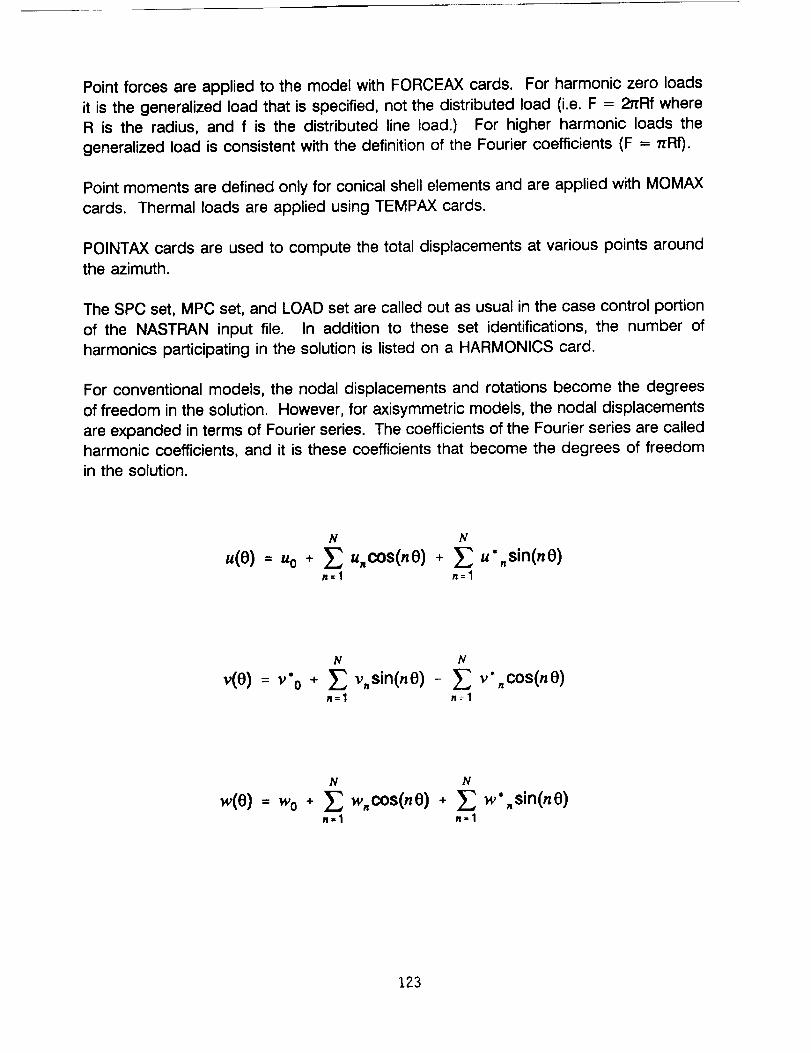
Point forces are applied to the model with FORCEAX cards. For harmonic zero loads
it is the generalized load that is specified, not the distributed load (i.e. F = 2nRf where
R is the radius, and f is the distributed line load.) For higher harmonic loads the
generalized load is consistent with the definition of the Fourier coefficients (F = _Rf).
Point moments are defined only for conical shell elements and are applied with MOMAX
cards. Thermal loads are applied using TEMPAX cards.
POINTAX cards are used to compute the total displacements at various points around
the azimuth.
The SPC set, MPC set, and LOAD set are called out as usual in the case control portion
of the NASTRAN input file. In addition to these set identifications, the number of
harmonics participating in the solution is listed on a HARMONICS card.
For conventional models, the nodal displacements and rotations become the degrees
of freedom in the solution. However, for axisymmetric models, the nodal displacements
are expanded in terms of Fourier series. The coefficients of the Fourier series are calledharmonic coefficients, and it is these coefficients that become the degrees of freedom
in the solution.
u(O)= Uo +
R' N
u.cos(nO) + _ u'.sin(ne)n=l n=l
N N
v(O) = v" 0 + _ v, sin(n0) - _ v',cos(ne)n=l n=l
w(O)= wo +N N
w.cos(nO) + _ w'.sin(nO)n=l n=l
123
The series are subdivided further into symmetric and anti-symmetric displacements with
respect to the e = 0 plane. The User's Manual refers to the symmetric and
anti-symmetric series as the "unstarred" and "starred" series respectively. The "starred"
series is indicated by the asterisk in the above equations. A complete solution to an
arbitrary problem consists of both "starred" and "unstarred" solutions. The type of
solution is specified on an AXlSYM card, either "cosine" (unstarred) or "sine" (starred).
These cannot be executed at the same time; these must be separate jobs. The resultsmust be combined external to NASTRAN.
The trapezoidal ring element has some limitations in defining its connections. The four
corner rings that define the element must be numbered counterclockwise. The bottom
and top edges (R1 to R2, and R3 to R4) of the element must be parallel to the radial
axis. The triangular ring element must have its corner rings specified counterclockwise.
These limitations are not prohibitive, but they must be recognized in the planning stage.
Axisymmetric elements are not compatible with conventional elements in the COSMIC
NASTRAN library. All the card images that can be used in an axisymmetric analysis are
listed in the User's Manual on the page that describes the AXIC card (page 2.4-12)oNonetheless, the static solution uses rigid format 1 to assemble stiffness and load
matrices, apply boundary conditions and multi-point constraints, solve the equations, and
compute forces and stresses. This is because the NASTRAN Preface sets up an
internally compatible numbering system. BANDIT is not used in this procedure.
The standard displacement output format is available to the user, but, the displacement
output consists of the harmonic coefficients. Total displacements can be obtained at
selected azimuthal positions specified on POINTAX cards.
Only the bending and shear forces are computed for the conical shell element. These
include the bending moment about the azimuthal axis, bending moment about the radial
axis, and the twisting moment. Also the radial and hoop shear forces are computed.
The radial, circumferential (hoop), and axial forces are computed at each ring location
for the solid axisymmetric elements.
These force quantities are output in harmonic form, that is, they are essentially harmoniccoefficients of a Fourier series of the force distribution. The 0 th harmonic term has a
multiplier of 2_R and higher harmonics have a multiplier of _R. Additionally, the total
force is computed at the locations around the azimuth which were specified on the
PCONEAX card, PTRIAAX card, or PTRAPAX card.
124
The element stresses computed for the conical shell elements are the radial normal
stress and the hoop normal stress, which include bending stresses, and in-plane shear
stress. The element stresses computed for the solid axisymmetric elements are the
three normal stresses, radial, hoop, and axial, and three shear stresses. Like the forces,
all these stresses are output in harmonic form, but are summed for locations around the
circumference that are specified on the property cards.
3) Discussion of the Finite Element Models:
Several finite element models were generated to illustrate the use of axisymmetricelements.
A simple thin-walled cylinder, shown in figure 2a, was modeled in two ways: first with
conical shell elements, and then with two layers of trapezoidal solid elements (figures 2b
& 2c). These two models illustrate the representation of a simple axisymmetric structure.
A model of a generic rotor balance was set-up to help explain how an axisymmetric
model can be coupled to a non-axisymmetric model. The balance is shown in figure 3.
The relatively extensive axisymmetric parts of the structure are the upper balance ring,
a conical adaptor piece, and a top plate. Four flexure posts connect the upper balance
ring to the grounded base. This flexure arrangement is not axisymmetric. A mast is
connected to the top plate.
The flexures and the mast were modeled separately using bar elements as shown in
figure 4. The stiffness matrix from this model is combined with the stiffness matrix of thebalance model to obtain a unified solution.
_a) Modeling aspects:
Some important modeling aspects need to be considered when generating an
axisymmetric finite element model. Some aspects are obvious and pertain to any finite
element model. Others are specific to axisymmetric element modeling.
The finite element model should be detailed enough to represent sufficiently the stiffness
of the structure. When planning the finite element model keep in mind the limitations of
the finite elements. Axisymmetric solid elements need to be generated in a
counterclockwise fashion with the upper and lower edges parallel to the radius. Conical
shell elements have an extra degree of freedom (rotation) that is not defined in the solid
elements. This degree of freedom will have to be accounted for.
125
The model should not contain so many degrees of freedom as to become excessively
time consuming to solvel The total degrees of freedom are the number of degrees of
freedom per ring, times the number of rings, times the number of harmonics. So even
a simple finite element model can have very many degrees of freedom if the number of
harmonics is large. Currently in NASTRAN, the user is compelled to include in the
solution degrees of freedom corresponding to all harmonic numbers, up to and including
the highest harmonic number specified. This means that the solution may involve lower
harmonics that do not participate in the response.
There should be rings positioned at key locations on the model. These locations might
be places where loads are applied or the model is bounded. Rings will be needed at
levels where an axisymmetric portion of the structure is joined with a non-axisymmetric
part. Still other points might be locations where displacements, loads, stresses, or some
other computed output is desired.
3b) Simple cylinder model:
The two thin-walled cylinder models used to illustrate an axisymmetric finite element
model are briefly described here (figures 2b and 2c). The cylinder has a 86.614 mm (22
inch) radius and is 0.984 mm (0.25 inches) thick and 1.575 mm (4.0 inches) high. It is
made from steel with a modulus of elasticity of 196.5 GPa (28.5x10⁶ psi), and a
coefficient of thermal expansion of 10.8x10 .6 m/m°C (6.0x10 .6 in/in-°F). The cylinder is
restrained from axial growth, but not from radial growth. Two loading conditions were
applied to this structure, a uniform radial pressure of 172.37x10³ Pa (25 psi), and a
uniform temperature change of 55.6°C (100 °F).
The first model of the cylinder uses 20 conical shell elements to represent the structure.
The second model uses 16 trapezoidal solid elements. Five harmonics (0 through 4)
were specified for both analyses (though it was known that the structure would respond
to these loads in the 0 th harmonic only).
Boundary conditions were specified on the RINGAX cards for both models. Axial
displacement "w" was constrained at the mean radius for z = 0.
The pressure load was applied using FORCEAX point load cards. The generalized force
on one element is the pressure times the element surface area: F = (p)(2_R)(_.). Half
of this total element force is distributed at the nodes. For the shell model, the mean
radius, 22 inches, was used in the analysis, and for the solid model, the inside radius,
21.875 inches, was used.
126
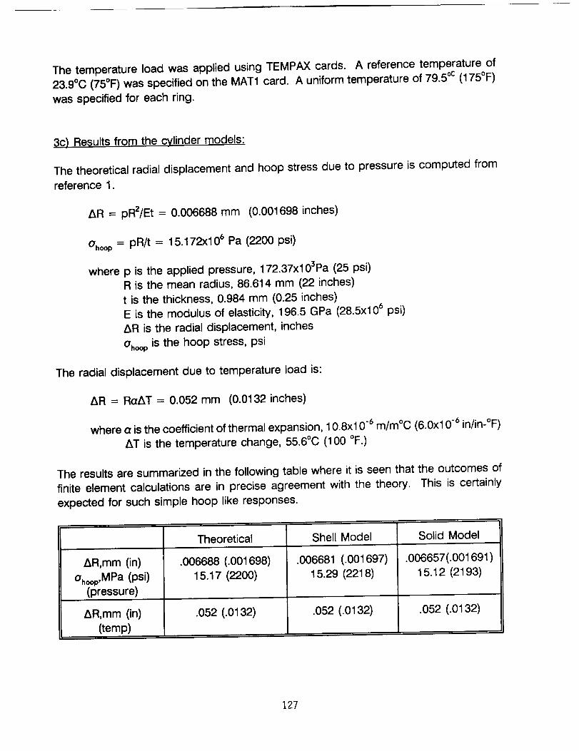
The temperature load was applied using TEMPAX cards. A reference temperature of
23.9°C (75°F) was specified on the MAT1 card. A uniform temperature of 79.5 °c (175°F)
was specified for each ring.
3c) Results from the cylinder models:
The theoretical radial displacement and hoop stress due to pressure is computed from
reference 1.
AR = pRZ/Et = 0.006688 mm (0.001698 inches)
Ohoop = pR/t = 15.172x10⁶ Pa (2200 psi)
where p is the applied pressure, 172.37x10³Pa (25 psi)
R is the mean radius, 86.614 mm (22 inches)
t is the thickness, 0.984 mm (0.25 inches)
E is the modulus of elasticity, 196.5 GPa (28.5x10⁶ psi)
AR is the radial displacement, inches
Ohoop is the hoop stress, psi
The radial displacement due to temperature load is:
AR = RoAT = 0.052 mm (0.0132 inches)
where o is the coefficient of thermal expansion, 10.8xl 0 .6 m/m°C (6.0xl 0 .6 in/in-°F)
AT is the temperature change, 55.6°C (100 °F.)
The results are summarized in the following table where it is seen that the outcomes of
finite element calculations are in precise agreement with the theory. This is certainly
expected for such simple hoop like responses.
AR,mm (in)
Ohoop,MPa (psi)(pressure)
AR,mm (in)
(temp)
Theoretical
.006688 (.001698)
15.17 (2200)
.052 (.0132)
Shell Model
.006681 (.001697)
15.29 (2218)
.052 (.0132)
Solid Model
.006657(.001691 )
15.12 (2193)
.052 (.0132)
127
:_1) Balance axisymmetric finite element model:
The upper balance ring is a five inch high, two inch thick cylinder with a mean radius of
39.37 mm (10 inches). The 1.476 mm (0.375 inch) conical adaptor section connects the
balance ring to the 1.476 mm (0.375 inch) top plate, which has a hole in its center. Thebalance material is stainless steel.
There are 10 TRAPAX elements representing the upper balance ring, 8 CONEAX
elements that model the conical adaptor piece, and 8 elements (5 TRAPAX and 3
TRIAAX) that make up the top plate. There are 39 rings and 4 harmonics specified
(starting with harmonic zero). This makes a total of 591 unconstrained degrees of
freedom. There are multi-point constraints between balance ring and cone, and between
cone and top plate to relate the rotational degree of freedom of the conical shell
elements to displacement degrees of freedom of the solid elements. Because the loads
are symmetric with respect to the e = 0 plane, the cosine solution (unstarred series) issufficient to solve the problem.
4) Mixed model procedure:
The overall approach to combining axisymmetric models with non-axisymmetric models
is to compute the separate stiffness matrices, then combine them to solve the coupled
problem. For this example two finite element models were generated, the axisymmetric
balance model, (figure 3), and the cartesian mast/flexure model, (figure 4).
There are four steps to the procedure. DMAP alter sequences are listed in the appendix.
1) Assemble the axisymmetric balance model global stiffness matrix and
output it to a file. Stop the solution process of this model at this point.
2) Specify external loads applied to the mast/flexure model and obtain the
global load and stiffness matrices for both the mast and balance flexures.
3) Read the previously stored balance stiffness matrix into the mast/flexure
model. Combine the stiffness matrices from both models using multi-point
constraint equations to express compatibility, and solve the problem.
Compute displacements and forces, and output the solution vector(s) toa file.
4) Read the solution vector(s) into the balance model. Continue the
problem and compute the axisymmetric element forces and stresses.
128
The key to combining models is to create an array space in the cartesian model that
corresponds to the size of the stiffness matrix of the axisymmetric model. This is done
by adding phantom grid points to the cartesian model. (Phantom grid points are not
connected to any structure; they just provide for space in the stiffness matrix.) Grid
points that correspond to the non-axisymmetric structure should be removed from the
solution set by OMIT cards. Grid points common to both structures are connected with
MPC relations. The remaining degrees of freedom in the cartesian model should
correspond exactly to those of the axisymmetric model.
For example, consider an axisymmetric problem with five harmonics specified in the
solution (0 through 4) coupled to a non-axisymmetric model in cartesian space.
Corresponding to a particular ring in the axisymmetric model, for instance ring number
4, there would be a set of phantom grid points in the cartesian model. These grid points
would be numbered, 10004, 11004, 12004, 13004, 14004 in the cartesian model to
represent the degrees of freedom of the five harmonics. Rotational degrees of freedom
4, 5, and 6 would be eliminated for all five "phantom" grid points, because axisymmetric
solid elements do not have rotational degrees of freedom. Additionally, degree of
freedom 2 for grid point 10004 is eliminated since it is not defined for the 0 t" harmonic
in the unstarred solution set. The remaining phantom degrees of freedom have no
elements attached to them and are flagged as singularities in the solution. This is
allowed because the solution process is modified by adding the stiffness matrix from the
axisymmetric model. Stiffness becomes associated with each of these degrees offreedom.
This procedure is straightforward, but it has the disadvantage that file space for two very
large matrices must be allocated.
Alternative approaches to combining axisymmetric and non-axisymmetric models were
considered. These made use of partitioning routines to extract and combine the
necessary information from the stiffness matrices. While these had the advantage of
being able to choose the stiffness terms associated with specific harmonics (and thus
store smaller matrices), these procedures were not as direct as the one outlined above.
4a) Multi-point constraints:
Two types of multi-point constraints are addressed here, MPC's at specific points around
the azimuth, and MPC's at every point around the azimuth.
129
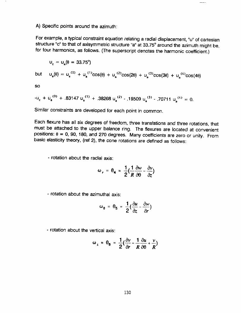
A) Specific points around the azimuth:
For example, a typical constraint equation relating a radial displacement, "u" of cartesian
structure "c" to that of axisymmetric structure "a" at 33.75 ° around the azimuth might be,
for four harmonics, as follows. (The superscript denotes the harmonic coefficient.)
but
SO
u c = ua(O = 33.75 °)
u.(e) = u. C°_+ ua(l_cos(O) + ua(2_cos(2e) + u.C3_cos(36) + u.(_cos(40)
-uc + u. C°_+ .83147 u. c1_ + .38268 u. c2_- .19509 uaC3_- .70711 Uac4_ = O.
Similar constraints are developed for each point in common.
Each flexure has all six degrees of freedom, three translations and three rotations, that
must be attached to the upper balance ring. The flexures are located at convenient
positions: e = O, 90, 180, and 270 degrees. Many coefficients are zero or unity. From
basic elasticity theory, (ref 2), the cone rotations are defined as follows:
- rotation about the radial axis:
1leVy
- rotation about the azimuthal axis:
I a. _)°_e = 05 = -2(& ar
- rotation about the vertical axis:
lo_ lau v
130
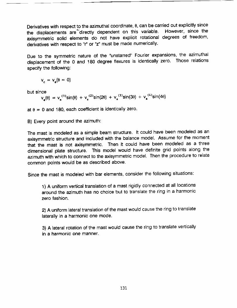
Derivatives with respect to the azimuthal coordinate, e, can be carried out explicitly since
the displacements are"directly dependent on this variable. However, since the
axisymmetric solid elements do not have explicit rotational degrees of freedom,
derivatives with respect to "r" or "z" must be made numerically.
Due to the symmetric nature of the "unstarred" Fourier expansions, the azimuthal
displacement of the 0 and 180 degree flexures is identically zero. Those relations
specify the following:
vc = v.(0= 0)
but since
vo(O) = v,¢l_sin(e) + v,¢2_sin(20) + v,¢3_sin(30) + v,¢4_sin(40)
at e = 0 and 180, each coefficient is identically zero.
B) Every point around the azimuth:
The mast is modeled as a simple beam structure. It could have been modeled as an
axisymmetric structure and included with the balance model. Assume for the moment
that the mast is not axisymmetric. Then it could have been modeled as a three
dimensional plate structure. This model would have definite grid points along the
azimuth with which to connect to the axisymmetric model. Then the procedure to relate
common points would be as described above.
Since the mast is modeled with bar elements, consider the following situations:
1) A uniform vertical translation of a mast rigidly connected at all locations
around the azimuth has no choice but to translate the ring in a harmonic
zero fashion.
2) A uniform lateral translation of the mast would cause the ring to translate
laterally in a harmonic one mode.
3) A lateral rotation of the mast would cause the ring to translate verticallyin a harmonic one manner.
131
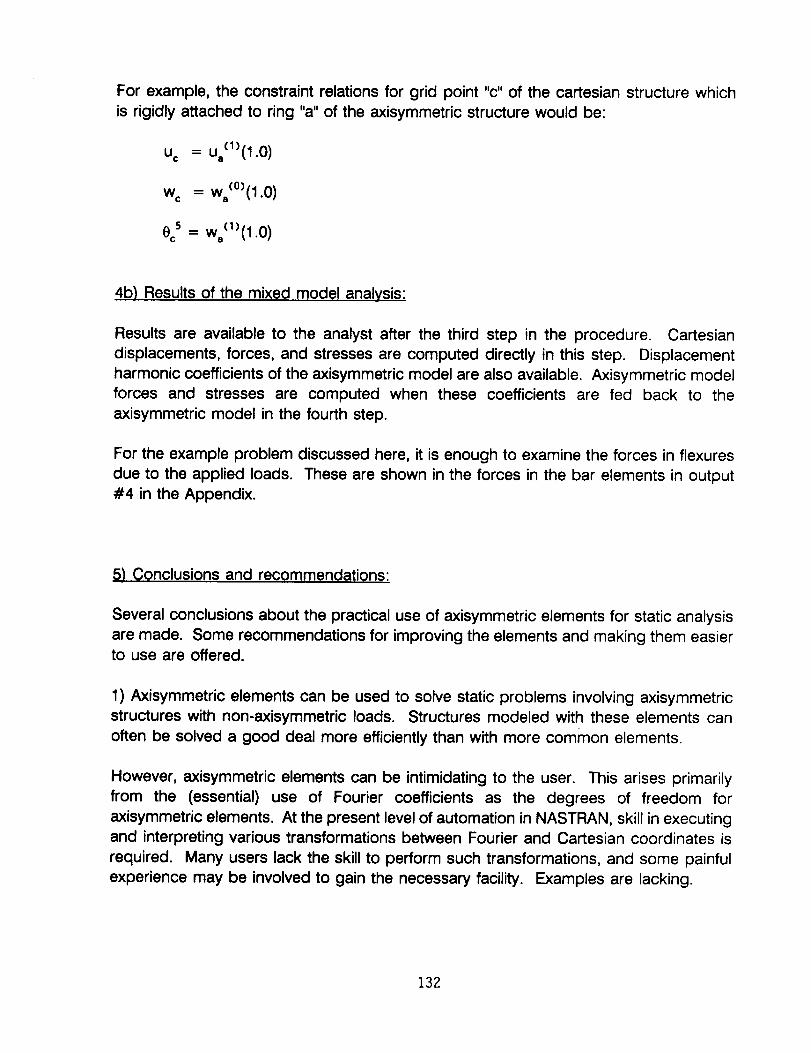
For example, the constraint relations for grid point "c" of the cartesian structure which
is rigidly attached to ring "a" of the axisymmetric structure would be:
u c = Uo(1)(1.0)
wc = wo(°)(1.0)
ec5 = w,(1)(1.0)
4b) Results of the mixed model analysis:
Results are available to the analyst after the third step in the procedure. Cartesian
displacements, forces, and stresses are computed directly in this step. Displacement
harmonic coefficients of the axisymmetric model are also available. Axisymmetric modelforces and stresses are computed when these coefficients are fed back to the
axisymmetric model in the fourth step.
For the example problem discussed here, it is enough to examine the forces in flexures
due to the applied loads. These are shown in the forces in the bar elements in output#4 in the Appendix.
_i) Conclusions and recommendations:
Several conclusions about the practical use of axisymmetric elements for static analysis
are made. Some recommendations for improving the elements and making them easierto use are offered.
1) Axisymmetric elements can be used to solve static problems involving axisymmetric
structures with non-axisymmetric loads. Structures modeled with these elements can
often be solved a good deal more efficiently than with more common elements.
However, axisymmetric elements can be intimidating to the user. This arises primarily
from the (essential) use of Fourier coefficients as the degrees of freedom for
axisymmetric elements. At the present level of automation in NASTRAN, skill in executingand interpreting various transformations between Fourier and Cartesian coordinates is
required. Many users lack the skill to perform such transformations, and some painful
experience may be involved to gain the necessary facility. Examples are lacking.
132
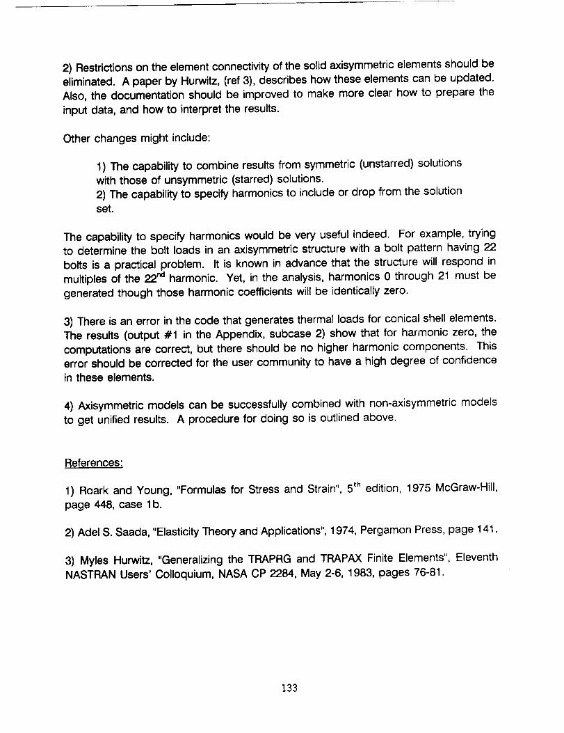
2) Restrictions on the element connectivity of the solid axisymmetric elements should be
eliminated. A paper by Hurwitz, (ref 3), describes how these elements can be updated.
Also, the documentation should be improved to make more clear how to prepare the
input data, and how to interpret the results.
Other changes might include:
1) The capability to combine results from symmetric (unstarred) solutions
with those of unsymmetric (starred) solutions.
2) The capability to specify harmonics to include or drop from the solutionset.
The capability to specify harmonics would be very useful indeed. For example, trying
to determine the bolt loads in an axisymmetric structure with a bolt pattern having 22
bolts is a practical problem. It is known in advance that the structure will respond in
multiples of the 22 r_ harmonic. Yet, in the analysis, harmonics 0 through 21 must be
generated though those harmonic coefficients will be identically zero.
3) There is an error in the code that generates thermal loads for conical shell elements.
The results (output #1 in the Appendix, subcase 2) show that for harmonic zero, the
computations are correct, but there should be no higher harmonic components. This
error should be corrected for the user community to have a high degree of confidencein these elements.
4) Axisymmetric models can be successfully combined with non-axisymmetric models
to get unified results. A procedure for doing so is outlined above.
References:
1) Roark and Young, "Formulas for Stress and Strain", 5 th edition, 1975 McGraw-Hill,
page 448, case lb.
2) Adel S. Saada, "Elasticity Theory and Applications", 1974, Pergamon Press, page 141.
3) Myles Hurwitz, "Generalizing the TRAPRG and TRAPAX Finite Elements", Eleventh
NASTRAN Users' Colloquium, NASA CP 2284, May 2-6, 1983, pages 76-81.
133
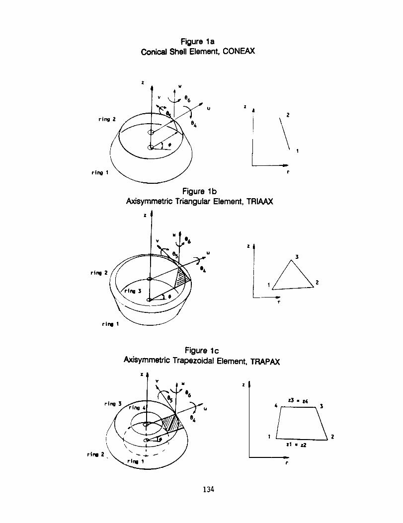
Figure laConical Shell Element, CONEAX
ZW
v _._ e6
U Z
Figure 1b
AxJsymmetric Triangular Element, TRIAAX
2
r
rinll 1
r
Figure lc
Axisymmetric Trapezoidal Element, TRAPAX
Z
V
e6
ring ] ri_ 4 "" _ u
zl-z2
r
134
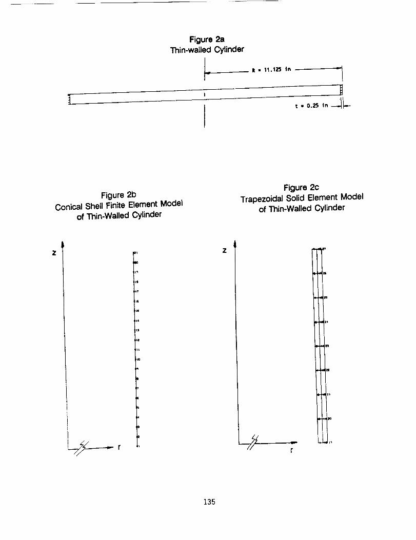
Figure 2a
Thin-walled Cylinder
It - 11.125 In
,-0.,5,°-_L
Figure 2bConical Shell Finite Element Model
of Thin-Walled Cylinder
Figure 2c
Trapezoidal Solid Element Model
of Thin-Walled Cylinder
Z;It
ttl
I17
;I
II
14
Itt
lit
'iO
Z
r
i
I!
I°II
I
I._1:_
135
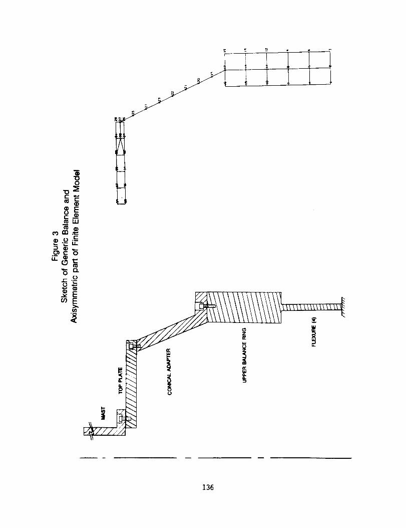
D
®130
c_
®E0c__W
_-_ E.
,,- r_0
r- ._-
136
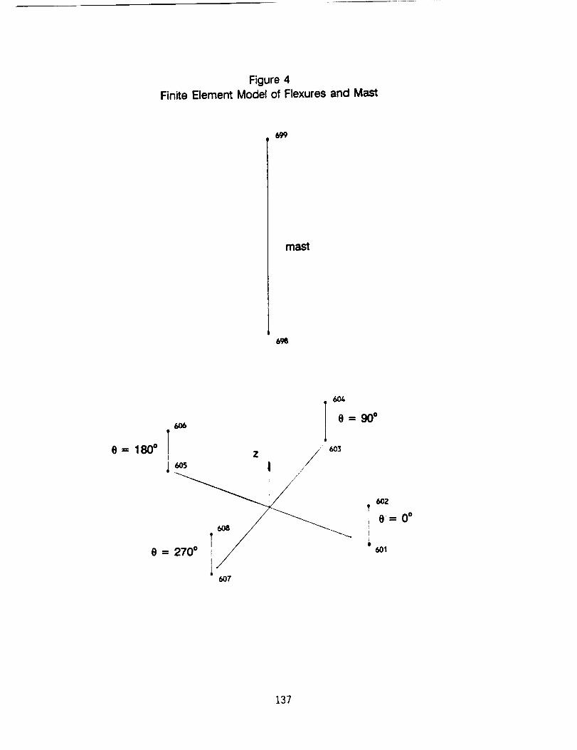
Figure 4Finite Element Model of Flexures and Mast
mast
fR8
6°6 I 0=90°
O= 180 ° _ z I //' _]
_ 0-0 °
0 = 270' / ' _1
i//6O7
137
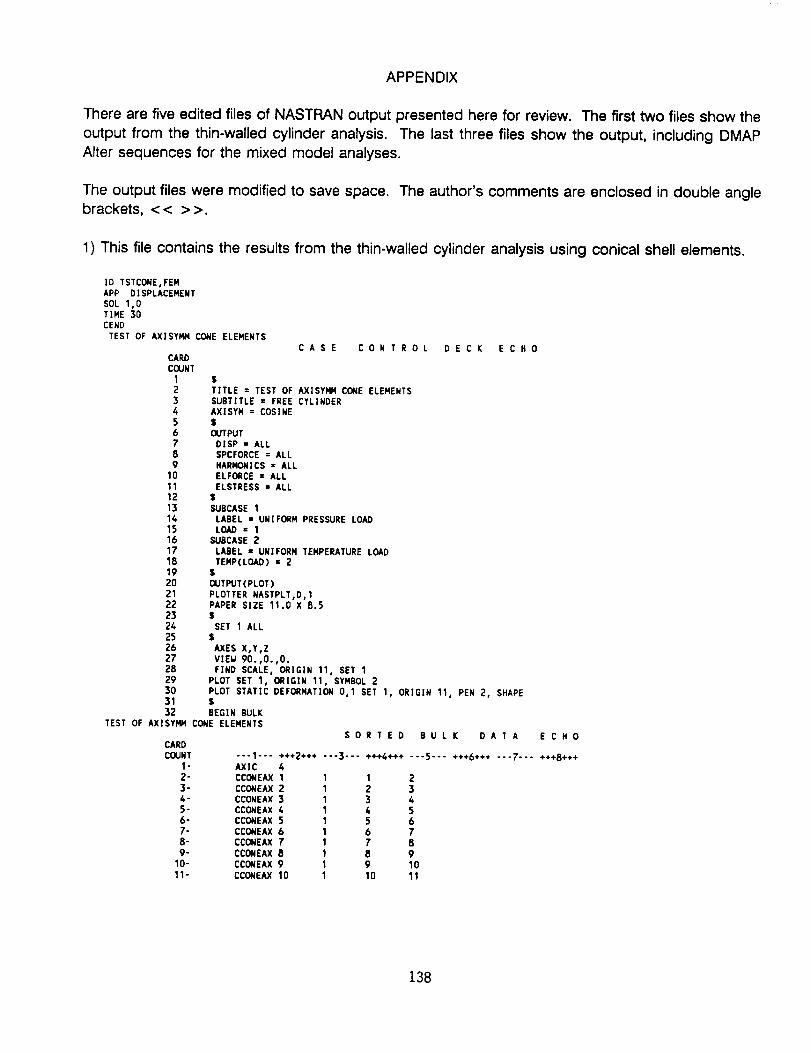
APPENDIX
There are five edited files of NASTRAN output presented here for review. The first two files show the
output from the thin-walled cylinder analysis. The last three files show the output, including DMAPAlter sequences for the mixed model analyses.
The output files were modified to save space. The author's comments are enclosed in double anglebrackets, < < > >.
1) This file contains the results from the thin-walled cylinder analysis using conical shell elements.
]D TSTCONE,FENAPP DISPLACEMENTSOL 1,0TIME 30CEND
TEST OF AXISYMM CONE ELEMENTS
CARDCOUNT
12345678
91011121314151617181920
2122232425262728293031
32
CASE CONTROL DECK ECHO
$TITLE = TEST OF AXISYMH CONE ELEMENTSSUBTITLE = FREE CYLINDERAXISYH = COSINE$OUTPUT
DISP = ALLSPCFORCE = ALLHARMONICS = ALLELFORCE = ALLELSTRESS = ALL
$SUBCASE 1
LABEL • UNIFORM PRESSURE LOADLOAD = 1
SUBCASE 2
LABEL • UNIFORH TEHPERATURE LOADTENP(LOAD) • 2
$
OUTPUT(PLOT)
PLOTTER NASTPLT,D,1PAPER SIZE 11.0 X 8.5$
SET 1 ALL$
AXES X,Y,ZVIEW 90.,0.,0.FIND SCALE, ORIGIN 11, SET 1
PLOT SET 1, ORIGIN 11, SYMBOL E
PLOT STATIC DEFORMATION 011 SET 1, ORIGIN 11, PEN 2, SHAPE$BEGIN BULK
TEST OF AX]SYMM CONE ELEMENTS
CARDCOUNT ---1--- +++2+++ -
1- AXIC 42- CCONEAX 1 13- CCONEAX 2 I4- CCONEAX 3 15- CCONEAX 4 16- CCONEAX 5 17- CCONEAX 6 18- CCONEAX 7 1
9- CCONEAX 8 1I0- CCOREAX 9 I11- CCONEAX 10 1
SO
°°3...
RTED BULK DATA ECHO
+++4+++ ---5--- +++6+++ ---7--- +++8+++
1 22 33 4
4 55 6
6 77 B8 99 10
10 11
138
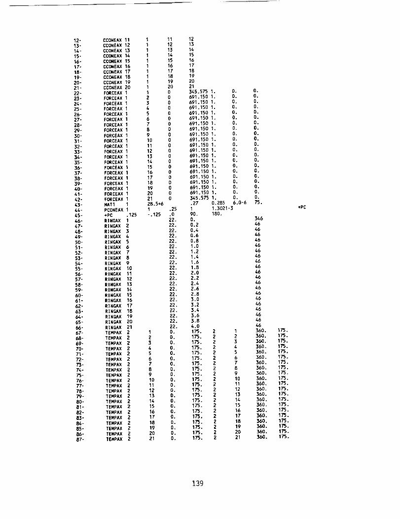
12-13-14-15-16-17-18-19-20-21-22-23-24-25-
26-27-
28-29-30-31-
32-33-34-35-36-37-38-39-40 °41-42-43 °44-45-
46-47-48-49-50-51-
52-53-54-55-56-57-58-59-60-61-
62-63-64-65-
66-67-
68-69-70-71-7'2-73-7'4-75-76-77-78-79-
80-81-82-
83-84-85-86-87-
CCONEAX 11CCONEAX 12CCONEAX 13CCONEAX 14CCONEAX 15CCONEAX 16CCONEAX 17CCO_IEAX 18
CCONEAX 19CCONEAX 20
FORCEAX 1FORCEAX 1FORCEAX 1FORCEAX 1FORCEAX 1FORCEAX 1FORCEAX 1FORCEAX 1
FORCEAX 1FORCEAX 1FORCEAX 1FORCEAX 1FORCEAX 1FORCEAX 1FORCEAX 1
FORCEAX 1FORCEAX 1FORCEAX 1FORCEAX 1FORCEAX 1FORCEAX 1NAT1 1PCONEAX 1+PC .125RINGAX 1RINGAX 2
R]NGAX 3RINGAX 4RINGAX 5RINGAX 6RINGAX TRINGAX 8
R[NGAX 9R[NGAX 10
RINGAX 11R[NGAX 12RINGAX 13RINGAX 14RINGAX 15RINGAX 16RINGAX 17
RINGAX 18R]NGAX 19RINGAX 20RINGAX 21TEMPAX 2TEMPAX 2TEMPAX 2
TEMPAX 2TEMPAX 2TEMPAX 2TEMPAX 2TEMPAX 2TEMPAX 2TEMPAX 2TEMPAX 2TEMPAX 2TEMPAX 2TEMPAX 2TEMPAX 2
TEMPAX 2TEMPAX 2TEMPAX 2TEMPAX 2TEMPAX 2
TEMPAX 2
11
11
1111111234567
89101112
1314
1516171819202128.5+61-.125
I
23
4
5
6
7
8
9
10
11
12
13
14
15
16
17
18
19
20
21
11 12
12 13
13 14
14 15
15 16
16 17
17 18
18 19
19 20
20 21
0 345.575 I.
0 691.150 1
0 691.150 10 691.150 1
0 691.150 10 691.150 1
0 691.150 1
0 691.150 1
0 691.150 1
0 691.150 1
0 691.150 1
0 691. 150 I.
0 691.150 I.
0 691.150 I.
0 691.150 I.
0 691.150 I.
0 691.150 I.
0 691.150 1.
0 691.150 I.
0 691.150 I.
0 345.575 1.
.27.25 1
.0 90.22. O.22. 0,222. 0.4
22. 0.6
22. 0.822. 1.022. 1.222. 1.4
22. 1.6
22. 1.8
22. 2.022. 2.222. 2.4
22. 2.622. 2.822. 3.022. 3.222. 3.4
22. 3.6
22. 3.8
22. 4.0
O. 175. 2O. 175. 2O. 175. 2
O. 175. 2O. 175. 2O. 175. 2O. 175. 2O. 175. 2
O. 175. 2O. 175. 2O. 175. 2O. 175. 2O. 175. 2O. 175. 2O. 175. 2
O. 175. 2O. 175. 2O. 175. 20. 175. 20. 175. 2O. 175. 2
0.285
1.3021-3
180.
O.
O.O.
O.O.O.O.O.O.O.
O.O.O.O.O.O.O.O.
O.O.
O.6.0-6
1
23
456789101112131415
1617181920
21
O.
O.O.O.O.O.O.O.
O.O.O.O.O.O.O.
O.O.O.O.O.O.75.
346
46
46
46
46
46
46
46
46
46
46
46
46
46
46
46
46
46
46
46
46
360.
360.360.360.360.360.360.360.360.
360.
360.
360.
360.
360.360.
360.360.360.
360.360.360.
175.175.17'5.175.175.175.175.175.175.
175.175.
175.175.175.175.175.175.
175.175.175.173.
+PC
139
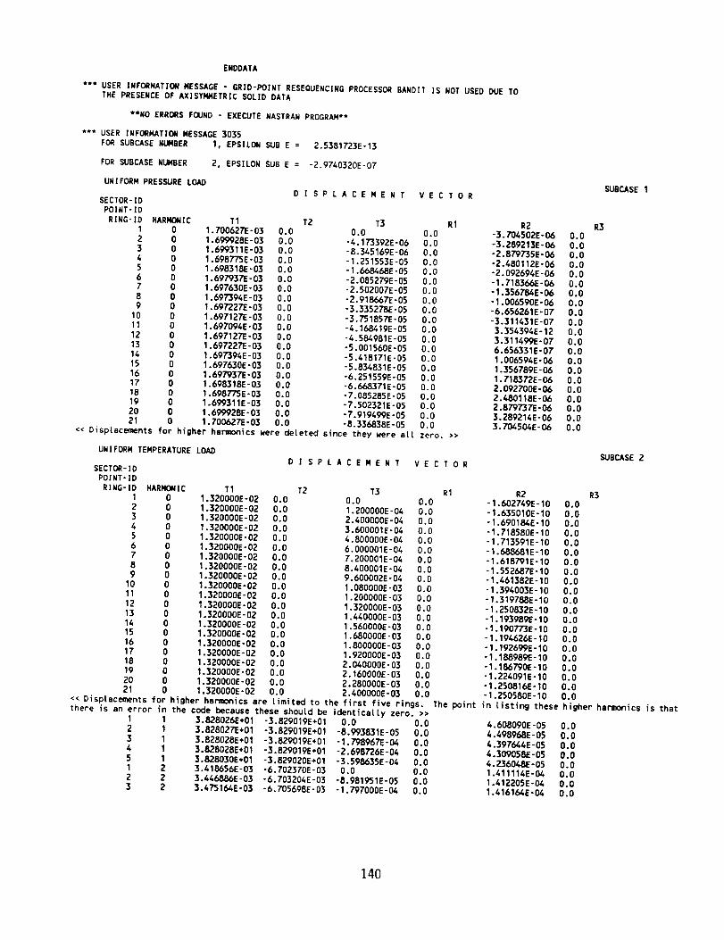
ENDDATA
*** USER INFORMATION NESSAGE - GRID-PO;NT RESEQUENCING PROCESSOR BANDIT IS NOT USED DUE TOTHE PRESENCE OF AXISYNHETRIC SOLID DATA
**NO ERRORS FOUND " EXECUTE NASTRAN PROGRAN**
*** USER INFORMATION NESSAGE 3035
FOR SUBCASE NUNBER 1, EPSILON SUB E = 2.5381723Eo13
FOR SUBCASE NUNBER
UNIFORN PRESSURE LOAD
SECTOR-IDPOINT-IDRING-ID
1234567
89
101112131415161T18192021
2, EPSILON SUB E = -2.9740320E-07
<< Displacements for
DISPLACEMENT VECTOR
HARNONIC T1 T2 T3 RI0 1.700627E-03 0.0 0.0 0,00 1.699928E-03 O.O -4.173392E-06 0.00 1.699311E-03 0.0 -8.345169E-06 0,00 1.698775E-03 0.0 -1.251553E-05 0.00 1.698318E-03 0.0 -1.668468E-05 0.0O 1.697937E-03 0.0 -2.085279E-05 0.0
0 1.697630E-03 0.0 -2.502007E-05 0.00 1.697394E-03 0.0 -2,918667E-05 0.00 1.697227E-03 0.0 -3.335278E-05 0.00 1.697127E-03 0.0 -3.751857E-05 O.O0 1.697094E-03 0.0 -4.168419E-05 0.00 1.697127E-03 0.0 -4.58k981E-05 0.00 1.697227E-03 0.0 -5.001560E-05 0.00 1.697394E-03 0.0 -5.418171E-05 0.0
0 1.697630E-03 0.0 -5.834831E-05 0.00 1.697937E-03 0.0 -6.251559E-05 0.00 1.698318E-03 0.0 -6.668371E-05 0.0
0 1.698775E-03 O.O -7.085285E-05 0.00 1.699311E-03 0.0 -7.502321E-05 0.00 1.699928E-03 0.0 -7.919499E-0S 0.00 1.700627E-03 0.0 -8.336838E-05 0.0
higher harmonics uere deleted since they were all zero. >>
DISPLACEMENTUNIFORN TENPERATURE LOAD
VECTORSECTOR-ID
POINT-IDRING-tO HARNONIC T1 T2 T3
1 0 1.320000E-02 0.0 0.0 0.02 0 1.320000E-02 0.0 1.200000E-04 0.0
3 0 1.320000E-02 0.0 2.400000E-04 0.04 0 1.320000E-02 0.0 3.600001E-04 0.05 0 1.320000E-02 0.0 4.800000E-04 0.06 0 1.320000E-02 0.0 6.000001E-04 0.07 0 1.320000E-02 O.O 7.200001E-04 0.08 0 1.320000E-02 0,0 8.400001E-04 0.09 O 1.320000E-02 0.0 9.600002E-04 0.0
10 0 1.320000E-02 0.0 1.080000E-03 0.011 0 1.320000E-02 0.0 1.200000E-03 0.0
12 0 1.320000E-02 0,0 1,320000E-03 0.013 O 1.320000E-02 0.0 1.440000E-03 0.014 0 1.320000E-02 0.0 1.560000E-03 0.015 0 1.320000E-02 0.0 1.(>80000E-03 0.016 0 1.320000E-02 0.0 1.800000E-03 0.017 0 1.320000E-02 0.0 1.920000E-03 0.018 0 1.320000E-02 0.0 2.040000E-03 0.019 0 1.320000E-02 0.0 2.160000E'03 0.020 0 1.320000E-02 0.0 Z.280000E-03 0.021 0 1.320000E-02 0.0 2.400000E-03 0.0
<< Displacements for higher harmonics are Limited to the first five rings.there is an error in the code because these should be identically zero. >>
1 1 3.828026E+01 -3.829019E+01 0.0 0.02 1 3.828027E+01 -3.829019E+01 -8.993831E-05 0.03 1 3.828028E+01 -3.829019E+01 -1.798967E-04 0.04 I 3.828028E+01 "3.829019E+01 "2.6987E6E'04 0.0
5 1 3.828030E+01 -3.829020E+01 -3.598635E-04 0.01 2 3.418656E-03 -6.702370E-03 0.0 0.0
2 2 3.446886E-03 -6.703204E-03 -8.981951E-05 0.03 2 3.475164E-03 -6.705698E-03 -1.797000E-04 O.O
R2-3.704502E-06
-3.289213E-06-2.879735E-06
-2.480112E-06-2.092694E-06-1.718366E-06-1.356784E-06-1.006590E-06-6.656261E-07-3.311431E-073.354394E-12
3.311499E-076.656331E-071.006594E-061.356789E-061.718372E-062.092700E-062.480118E-062.8797371E-063.289214E-063.704504E-06
RI R2-1.602749E-I0
-1.635010E-10.6901_E-I0
- .718580E-10- .713591E-10-.688681E-10- .618791E-10-'.552687E-10- .461382E-10-'.394003E-10
- .319788E-10-,250832E-10- .193989E-10-'.19077"3E-10- ,194626E-10-1.192699E-10-1.188989E-10-1.186790E-10-1.224091E-10-1.250816E-10-1.250580E-10
The point in tisting these
4.608090E-054.498968E-05
4.397646E-054.309058E-054.Z36048E-O51.411116E-041.412205E-041.416164E-D4
SUBCASE 1
R30.0
O.O0.0
0.00.00.00.0O.O0.00.00.0
0.0O.O0.00.0O.O0.00.00.00.00.0
SUBCASE 2
R3O.O
0.00.00.00.00.0O.O0.00.00.0
0.00.00.00.00.00.00.00.00.0
0.00.0
higher harmonics is that
0.00.0
0.00.00.00.00.00.0
140
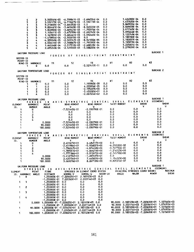
4 25 21 32 3
3 34 35 31 42 43 44 45 4
3.503561E-03 -6.709841E-03
3.532173E-03, -6.715627E-039.210605E-04 ;-3.664352E-03
9.824461E-04 -3.665628E-031.043900E-03 -3.669423E-031.105611E-03 -3.675709E-03
1.167805E-03 -3.684461E-03-1.470954E-04 -2.502015E-03
-4.339249E-05 -2.503747E-036.034414E-05 -2.508867E-031.645048E-04 -2.517312E-032.695243E-04 -Z.SE9030E-03
-2.696334E-04 0.0 1.424383E-04-3.596119E-04 0.0 1.437620E-04
0.0 0.0 3.069935E-04-8.963325E-05 0.0 3.069658E-04-1.793976E-04 0.0 3.077363E-04-Z.692745E-04 0.0 3.095646E-04
-3.592463E-04 0.0 3.125749E-04
0.0 0.0 5.189780E-04
-8.941032E-05 0.0 5.18303TE-04
-1.790392E-04 0.0 5.193919E-04
-2.688528E-04 0.0 5.225801E-04
-3.588200E-04 0.0 5.279839E-04
UNIFORM PRESSURE LOAD
SECTOR-IDPOINT-ID
RING-ID HARMONIC1 0 0.0
FORCES OF SINGLE-POINT CONSTRAINT
T1 T2 T3 R1 R20.0 -3.527417E-11 0.0 0.0
UNIFORM TEMPERATURE LOAD
SECTOR-IDPOINT'ID
RING-ID HARMONIC1 01 11 21 31 4
FORCES OF SINGLE-POINT CONSTRAINT
T1 T2 T3 R1 R20.0 0.0 1.193963E-09 0.0 0.0
0.0 0.0 4.233956E-05 0.0 0.00.0 0.0 -2.195207E+00 0.0 0.00.0 0.0 -3.430285E+01 0.0 0.00.0 0.0 -2.067654E+02 0.0 0.0
UNIFORM PRESSURE LOADFORCES I N
ELEMENT HARMO_IIC POINT
]D. NUMBER ANGLE1 0
1 11 21 31 41 0.00001 90.00001 180.0000
AXIS-SYMMETRIC CONICAL SHELLBEND-MOMENT BEND-MOMENT TWI ST-MOMENT
V U-7.SZI445E-01 -2. 030790E-01 0.0
0.0 0.0 0.0
0.0 0.0 0.0
0.0 0.0 0.0
0.0 0.0 0.0
-7.521445E-01 -2.030790E-01 0.0
-7.521445E-01 -2.030790E-01 0.0-7,521445E-01 -2. 030790E-01 0.0
ELEM
0.0
0.00.00.00.00.00.0
0.0
UNIFORM TEMPERATURE LOADFORCES I g
ELEMENT HARMONIC POINTID. NUMBER ANGLE
1 01 11 21 3
1 41 0.00001 90.00001 180.0000
AXIS-SYMMETRIC CONICAL SHELLBEND-MOHENT BEND-MOHENT TWI ST-MOMENT
V U2.401673E+01 6.484517E+00 0.0-2.451984E+01 "5.926837E+00 "6.250000E-02
-I. 796247E+01 -4.874458E+00 -3.707733E-01
"1.789051E+01 "4.644216E÷00 -1.216523E+00
"I. 777186E+01 -3.913975E+00 -2.745798E+00
"5.412794E+01 "I .287497E÷01 0.0
2.420734E÷01 7.445001E+00 I.154023E+00
3.069276E+01 8.267138E÷00 -9.905316E'07
ELEM
0.00.0
0.00.00.00.00.00.0
UNIFORM PRESSURE LOAD
STRESSESELEMENT POINT
ID. HARMONIC ANGLE1 0
1 1
1 2
1 3
1 4
1 0.0000 1
1 90.0000
1 180.0000
% N AXIFIBRE
S- SYMMET R I C CONICALSTRESSES IN ELEMENT COORD SYSTEM
DISTANCE NORHAL-V NORMAL-U SHEAR-UV1.250000E-01 -7.220625E+01 2.183123E+03 0.0
"1.250000E'01 7.220363E+01 2.222114E+03 0.01.250000E-01 0.0 0.0 0.0
"1.250000E'01 0.0 0.0 0.01.250000E-01 0.0 0.0 0.0
-1.250000E-01 0.0 0.01.250000E-01 0.0 0.0
-1.250000E-01 0.0 0.01.250000E-01 0.0 0.0
-1.250000E-01 0.0 0.0.250000E'01 -7.ZZO625E+01 2.183123E+03
0.00.00.00.0
0.00.0
-1.250000E'01 7.2ZO363E+01 2.222114E+03 0.01.250000E-01-7.220625E+01 2.183123E+03 0.0-1.250000E-01 7.220363E+01 2.222114E+03 0.01.250000E-01 -7.220625E*01 2.183123E+03 0.0
0.00.00.00.0
: 0.00.00.00.00.00.0
0.00.0
SUBCASE 1
R3
0.0
SUBCASE 2
R30.00.00.00.00.0
ENT SSHEAR
V
SUBCASE 1
(CCONEAX)SHEAR
U0.00.00.00.0
0.00.00.00.0
ENTSSHEAR
V
SUBCASE 2
(CCONEAX)SHEAR
U0.00.00.00.00.00.0
0.00.0
SUBCASE 1
S H E L L E L E M E N T S (CCONEAX)PRINCIPAL STRESSES (ZERO SHEAR) MAXIMUM
ANGLE MAJOR MINOR SHEAR
90.0000 2.183123E+03 -7.220630E+01 1.127665E+0390.0000 2.222114E+03 7.220361E+01 1.074955E+03
90.0000 2.183123E+03 -7.220630E+01 1.127665E+0390.0000 2.222114E+03 7.220361E+01 1.074955E+03
90.0000 2.183123E+03 -7.220630E+01 1.127665E+03
141

"1.250000E'01 7.220363E+01 2.222114E+03 0.0 90.0000 2.222114E+03 7.220361E+01 1.074955E+03
UNIFORM TENPERATURE LOADSTRESSES IN
ELEMENTID. HARNONIC
1 0
1 1
1 2
1 3
1 4
AXIS'SYMMETRIC CONICALPOINT FIBRE STRESSES IN ELEMENT COORD SYSTENANGLE DISTANCE NORMAL'V NORMAL-U SHEAR'UV
1.250000E'01 2.573024E+04 2.404717E+04 O.O-1.250000E-01 2.111908E+04 2.280215E+04 0.0
1.250000E-01 -1.992134E+04 -1.816540E+04 -5.999923E*00-1.250000E-01 -1.521359E+04 -1.702747E+04 5.999923E+00
1.250000E-01 -1.929200E+04 -1.813068E+04 -3.659378E+01-1.250000E-01 -1.58_385E+04 -1.719479E+04 3.459378E+01
1.250000E-01 -1.928362E+04 -1.819923E+04 -1.198160E+02-1.250000E-01 -1.584869E+04 -1.730755E+04 1.137535E+02
1.250000E-01 -1.926194E+04 -1.820866E+04 -2.695620E+02°1.250000E-01 °1.584978E÷04 -1.745718E+04 2.576245E+02
SUBCASE 2
S H E L L E L E N E N T S (CCONEAX)PRINCIPAL STRESSES (ZERO SHEAR) NAXIMUM
ANGLE NAJOR MINOR SHEAR
0.0000 1.250000E-01 -5.202926E+04 -4.865680E+04 0.0 90.0000 -6.865680E+04 -5.202926E+04 1.686227E+03-1.250000E-01 -4.163683E+04 -4.618484E+04 0.0 O.O000 -4.163683E+04 -4.618484E+04 2.274008E+03
90.0000 1.250000E-01 2.576090E+04 2.396919E+04 1.138160E+02 3.6202 2.576810E+04 2.396199E+04 9.030555E+02
-1.250000E-01 2.111315E+04 2.253977E+04 -1.077535E+02 -85.7049 2.254786E+04 2.110506E+04 7.214023E+02180.0000 1.250000E-01 2.638067E+04 2.407247E+04 -9.727959E-05 0.0000 2.638067E+04 2.407247E+04 1.154101E+03
-1.Z500DOE-01 2.048774E*04 2.248520E+04 9.290005E-05 90.0000 2.248520E+04 2.048774E+04 9.987316E+02
* * * END OF JOB * * *
2) This file contains the results of the thin-walled cylinder analysis using the trapezoidal solid elements.
[D TSTCYL,FENAPP DISPLACENENT
SOL 1,0TIME 60
$CEND
CARDCOUNT
12365
6789
101112131415
16171819202122232425
2627282930
CARDCOUNT
1-
CASE CONTROL DECK ECHO
TITLE = TEST CYLINDERSUBTITLE = UNIFORN PRESSURE$AXISYN = COSINE
OUTPUTDISPLACEMENTS = ALLSPCFORCES = ALLELFORCES = ALLELSTRESS = ALLHARNONICS = ALL
$SUBCASE 1
LABEL = PRESSURE LOAD
LOAD = 1SUBCASE 2
LABEL = UNIFORM TENPERATURE LOADTENPERATURE(LOAD) = 2
$OUTPUT (P LOT )
PLOTTER NASTPLT,D,1PAPER SIZE 11.0 X 8.5$
SET 1 ALL$
AXES X,Y,ZVIEW 90. ,90. ,0.FIND SCALE, ORIGIN 11, SET 1
PLOT SET 1, ORIGIN 11$BEGIN BULK
SORTED BULK DATA ECHO
"'-1"'- ++÷2+++ -"3-'" +++4+++ ""5-" +++6+++ ""7"-- +++8+++ -"9-" ++÷10+++AXIC 4
142
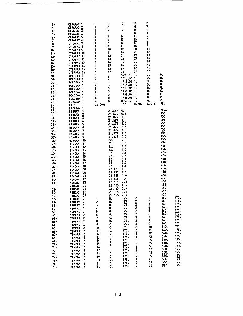
2-
3-4-5-6-7-8-9-
10-11-12-13-14-15-
16-17-18-19-20-21-
22-23-24-25-26-27-28-29-30-31-32-33-
34-55-56-37-38-39-40-41-
42-43-44-45-46-47-48-49-50-51-
52-53-54-55-
56-57-58-59-
60-61-
62-65-64-65-66-67-
68-69-70-71-72-73-74-
75-76-77-
CTRAPAX 1CTRAPAX 2CTRAPAX 3CTRAPAX 4
CTRAPAX 5CTRAPAX 6CTRAPAX 7CTRAPAX 8CTRAPAX 9CTRAPAX 10
CTRAPAX 11CTRAPAX 12
CTRAPAX 13CTRAPAX 14CTRAPAX 15CTRAPAX 16FORCEAX 1
FORCEAX 1FORCEAX 1FORCEAX 1FORCEAX 1FORCEAX 1FORCEAX 1FORCEAX 1FORCEAX 1MAT1 1PTRAPAX 1RINGAX 1RINGAX 2
R[NGAX 3R[NGAX 4RINGAX 5RINGAX 6RINGAX 7R]NGAX 8R]NGAX 9RXNGAX 10R]NGAX 11
R[NGAX 12RINGAX 13RINGAX 14RINGAX 15RINGAX 16RINGAX 17
R]NGAX 18R]NGAX 19
R[NGAX 20R]NGAX 21R[NGAX 22R|NGAX 23RINGAX 24R[NGAX 25
RINGAX 26R]NGAX 27TEMPAX 2TENPAX 2TEMPAX 2TEMPAX 2TEMPAX 2TEMPAX 2TEMPAX 2TEMPAX 2TEMPAX 2TEMPAX 2
TEMPAX 2TEMPAX 2TEMPAX 2TEMPAX 2TEMPAX 2TEMPAX 2TEMPAX 2TEMPAX 2
TEMPAX 2TEMPAX 2TEMPAX 2TEMPAX 2
I11111111111
1111
12345678928.5+6
12345678910
1112131415161718
19202122
123456781011121314151617
000000
000
121.87521.87521.87521.87521.87521.875
21.87521.87521.87522.22.22.22.
22.22.22.22.22.22.12522.12522.12522.125
22.12522.12522.12522.125
22.125O.O.O.O.
O.O.O.O.O.O.O.O.
O.O.O.O,
O.O.O.O.O.
O.
10 11
11 12
12 13
13 14
14 15
15 16
16 17
17 18
19 20
20 21
21 22
22 23
23 24
24 25
25 2626 27859.03 1.1718.06 1
1718.06 11718.06 11718.06 11718.06 11718.06 11718.06 1859.03.27
O.
0.51.0
1.52.02.53.03.54.0
O.0.5
1.01.52.02.53.03.54.0
O.0.51.01.52.02.53.0
3.54.0175.175.175.175.175.175.175.175.175.175.
175.175.175.175.175.175.175.175.175.
175.175.175.
1O. 285
23456789111213141516
1718O.O.O.
O.0.O.O.O.O.6.0-6
I
2
3
4
5
6
7
8
910
11
12
13
14
15
16
17
18
19
20
21
22
O.
O.O.O.O.O.
O.O.O.75.
3456456456456456456456
456456456456456456
456456
456456456456456456456456
456456456456
360.360.
360.360.360.360.360.360.360.360.360.360.360.360.
360.360.
360.360.360.360.360.360.
175.175.175.175.175.175.175.175.175.
175.175.175.175.175.175.175.175.175.175.
175.175.175.
143
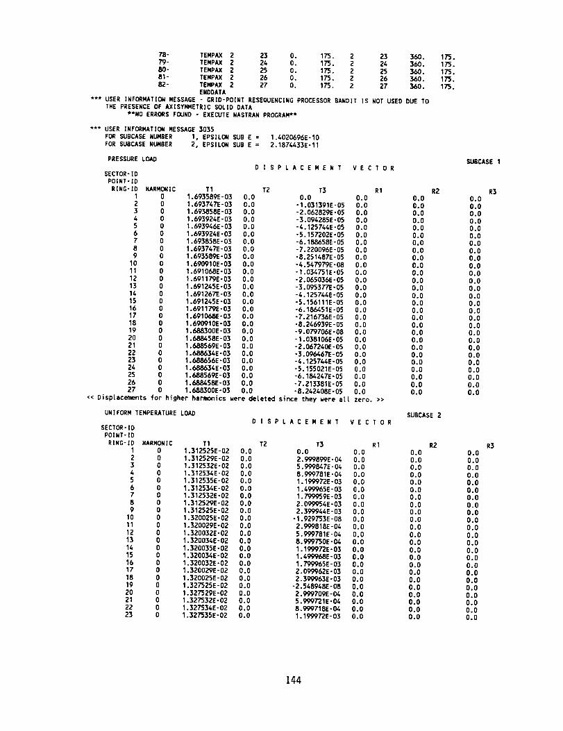
78- TEMPAX 2 23 0. 175. 2 23 360, 175.79- TEMPAX 2 24 O. 175. 2 24 360. 175.
80- TEMPAX 2 25 O. 175. 2 25 360. 1T5.81- TEMPAX 2 26 O. 175. 2 26 360. 175.
82- TEMPAX 2 27 O. 175. 2 27 360. 175.ENDDATA
*** USER INFORMATION MESSAGE - GRID-POINT RESEQUENCING PROCESSOR BANDIT IS NOT USED DUE TOTHE PRESENCE OF AXISYI_ETRIC SOLID DATA
**NO ERRORS FOUND - EXECUTE NASTRAN PROGRAM**
*** USER INFORMATION MESSAGE 3035
FOR SUBCASE NUMBER 1, EPSILON SUB E =FOR SUBCASE NUMBER 2, EPSILON SUB E =
PRESSURE LOAD
1.4020696E-102.1874433E-11
DISPLACEMENT VECTORSECTOR-ID
POINT-]D
RING-ID HARMONIC T1 T2 T3 R1 R21 0 1.693589E-03 0.0 0.0 0.0 0.0
2 0 1.693747E-03 0.0 -1.031391E-05 0.0 O.O3 0 1.693858E-03 0.0 -2.062829E-05 0.0 0.04 0 1.693924E-03 0.0 -3.094285E-05 0.0 0.05 0 1.693946E-03 0.0 -4.125744E-05 0.0 0.0
6 0 1.693924E-03 0.0 -5.157202E-05 0.0 0.07 0 1.693858E-03 0.0 -6.188658E-05 0.0 0.08 0 1.693747E-03 0.0 -7.220096E-05 0.0 0.09 0 1,693589E-03 0.0 -8.251487E-05 0.0 0.0
10 0 1.690910E-03 0.0 -4.547979E-08 0.0 0.011 0 1.691068E-03 0.0 -1.034751E-05 0.0 0.0
12 0 1.691179E-03 0.0 -2.065036E-05 0.0 0.013 0 1.691245E-03 0.0 -3.095377E-05 0.0 0.016 0 1.691267E-03 0.0 -4.125744E-05 0.0 0.015 0 1.691245E-03 0.0 -5.156111E-05 0.0 0.016 0 1.691179E-03 0.0 -6.186451E-05 0.0 0.017 O 1.691068E-03 0.0 -7.216736E-05 0.0 0.018 0 1.690910E-03 0.0 -8.246939E-05 0.0 0.019 0 1.688300E-03 0.0 -9.079706E-08 0.0 0.020 0 1.688458E-03 0.0 -1,038106E-05 0.0 0.021 0 1.688569E-03 0.0 -2.067260E-05 0,0 0.022 0 1.688634E-03 0.0 -3.096467E-05 0.0 0.023 0 1.688656E-03 0.0 -4.125744E-05 0.0 0.024 0 1.688634E-03 0.0 -5.155021E-05 0.0 0.025 0 1.688569E-03 0.0 -6.184247E-05 0.0 0.026 0 1,688458E-03 0.0 -7.213381E-05 0.0 0.027 0 1.688300E-03 0.0 -8.242408E-05 0.0 0.0
<< Displacements for higher harmonics were deleted since they were all zero. >>
UNIFORM TEMPERATURE LOAD SUBCASE 2DISPLACEMENT VECTOR
SECTOR-ID
POINT-ID
RING-ID HARMONIC T1 T2 T3 R1 R21 0 1.312525E-02 0.0 0.0 0.0 0.02 0 1.312529E-02 0.0 2.999899E-04 0.0 0.03 0 1.312532E-02 0.0 5.999847E-04 0.0 0.04 0 1.312534E-02 0.0 8.999781E-04 0.0 0.05 0 1.312535E-02 0.0 1.199972E-03 0.0 0.06 0 1.312534E-02 0.0 1.499965E-03 0.0 0.07 0 1.312532E-02 0.0 1.799959E-03 0.0 0.08 0 1.312529E-02 0.0 2.099954E-03 0.0 0.09 0 1.312525E-02 0.0 2.399944E-03 0.0 0.0
10 0 1.320025E-02 0.0 -1.929753E-08 0.0 0.011 0 1.320029E-02 0.0 2.999818E-04 0.0 0.0
12 0 1.320032E-02 0.0 5.999781E-04 0,0 0.013 0 1.320034E-02 0.0 8.999750E-04 0.0 0.014 0 1.320035E-02 0.0 1.19997ZE-03 0.0 0.015 0 1.320034E-02 0.0 1.499968E-03 0.0 0.016 0 1.320032E-02 0.0 1.799965E-03 0.0 0.017 0 1.320029E-02 0.0 2.0_62E-03 0.0 0.0
18 0 1.320025E-02 0.0 2,399963E-03 0,0 0.019 0 1.327525E-02 0.0 -2.548948E-08 0.0 0.0
20 0 1.327529E-02 0.0 2.999709E-04 0.0 0.021 0 1.327532E-02 0.0 5.999721E-04 0.0 0.022 0 1.327534E-02 0.0 8.999718E-04 0.0 0.023 0 1.327535E-02 0.0 1.199972E-03 0.0 0.0
SUBCASE 1
R30.0
0.00.00.00,00.00.00.00.00.00.00.0
0.00.00.00.00.00.00.00.00.00.00.00.00.00.00.0
R3
0.0
0.0
0.0
0.0
0.0
0.0
0.0
0.0
0.0
0.0
0.0
0.0
0.0
0.0
0.0
0.0
0.0
0.0
0.0
0.0
0°0
0.0
0.0
144
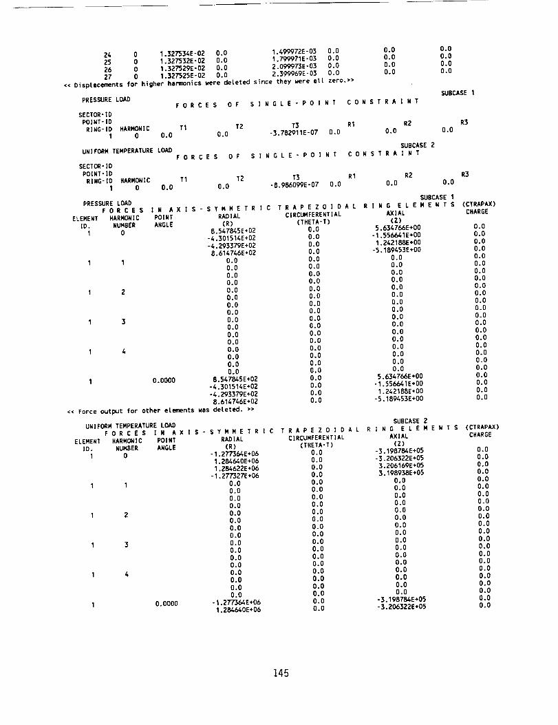
24 0 1.327534E-02 0.0 I.499972E -03 0.0 0.0 0.0
25 0 1.327532E-02 0.0 I.799971E- 03 0.0 0.0 0.0
26 0 1.327529E- 02 O.O 2.099973E- 03 0.0 0.0 0.0
27 0 1,327525E-02 0.0 2.399969E -03 O.O 0.0 0.0
<< Displacements for higher harmonics were deleted since they were all zero.>>
PRESSURE LOAD SUBCASE 1FORCES OF S] NGLE-POINT CONSTRAINT
SECTOR-IDP01NT-ID
RING-ID HARMONIC T1 T2 T3 R1 R2 R31 0 0,0 0.0 -3.782911E-07 0.0 0,0 0,0
SUBCASE 2
FORCES OF S I NG L E- PO I N T CONS T RA I N TUNIFORM TEMPERATURE LOAD
SECTOR-IDPOINT-1D
R|NG'ID HARMONIC T1 T2 T3 R1 R2I 0 0.0 0.0 -8.986099E-07 0.0 0.0 0.0
R3
PRESSURE L_D SUBCASE I
F 0 R C E S I N A X I S - S Y M M E T R I C T R A P E Z O I D A L R ] N G E L E M E N T S (CTRA_X)ELEMENT HARM_]C POINT RADIAL CIRCUMFERENTIAL _IAL CHARGE
ID, N_BER ANGLE (R) (THETA-T) (Z)1 0 8.547_5E+02 0,0 5.6347_E+00 0.0
-4.301514E+02 0.0 -I.556641E+00 0.0
-4.293379E+02 0.0 1.2421_E+00 0.08.614746E+02 0.0 -5.189453E+00 0.0
1 1 O.O 0,0 0.0 0.00.0 0.0 0.0 0.0
0.0 0.0 0.0 0.00.0 0.0 0.0 0.0
1 2 O.O 0.0 0.0 0.00.0 0.0 0.0 0.0
0.0 0.0 0.0 0.0
0.0 0.0 0.0 0.01 3 0.0 0.0 O.O 0.0
0.0 0.0 O.O O.O0.0 0.0 0.0 0.0O.O 0.0 0.0 0.0
1 4 0.0 0.0 0.0 0.00.0 0,0 0.0 0.00.0 0.0 0.0 0.00.0 0.0 0.0 0.0
1 0,0000 8.547_5E+02 0.0 5._47_E+00 0.0"4.301514E+02 0.0 -1.556641E+00 0.0"4.2933_E+02 0.0 1.242188E+00 0.08.614746E+02 0.0 -5.189453E+00 0.0
<< Force output for other etements was deteted. >>
UNIFORM TEMPERATURE LOAD SUBCASE 2
F O R C E S I N A X ] S " S Y M M E T R I C T R A P E Z O I D A L R [ N G E L E M E N T S (CTRAPAX)ELEMENT HARMONIC POINT RADIAL CIRCUMFERENTIAL AXIAL CHARGE
IO. NUMBER ANGLE (R) (THETA-T) (Z)I 0 - I. 27T'564E +06 0.0 - 3.198784E+05 0.0
I. 284640E+06 O, 0 - 3. 206322E+05 O. 0I.284622E+06 O.0 3.206169E+05 O. 0
"I. 277327E+06 O. 0 3.198938E+05 O. 0I I 0.0 0,0 0.0 0.0
0.0 0.0 0.0 0.00.0 0.0 0.0 0.0
0.0 0°0 0.0 0.0
I 2 0.0 0.0 0.0 0.0
0.0 0.0 0.0 0.0
0.0 0.0 0.0 0.00.0 0.0 0.0 0.0
I 3 0.0 0.0 0.0 0.0
0.0 0.0 0.0 0.0
0.0 0.0 0.0 0.0
0.0 0.0 0.0 0.01 4 0.0 0.0 O.O 0.0
0.0 0.0 0.0 0.0
0.0 0.0 0.0 0.00.0 O.O 0.0 0.0
1 O.O00O - 1.277364E+06 O. 0 -3,198784E÷05 O. 0I.284640E+06 0.0 "3. 206322E+05 0.0
145
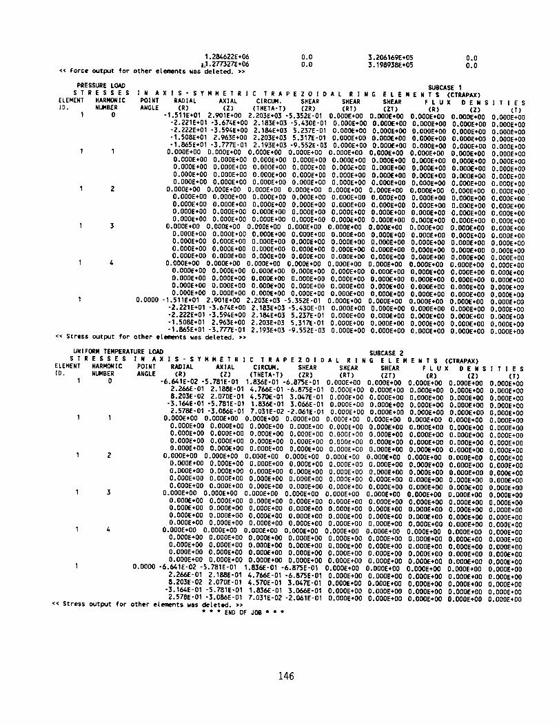
1.284622E+06 0.0 3.206169E+05 0.0
;_.2_2_+06 0.0 ].19893_+05 0.0<< Force output for other elements was deteted. >>
PRESSURE LOAD SUBCASE I
S T R E S S E S ; N A X I S - S Y N N E T R I C T R A P E Z O I D A L R I N G E L E N E N T S (CTRAPAX)ELEMENT HARMONIC PO%NT RADIAL AX%AL CIRCUN. SHEAR SHEAR SHEAR F L U X D E N S I T I E SID. NUMBER ANGLE (R) (Z) (THETA'T) (ZR) (RT) (ZT) (R) (Z) (T)
1 0 "1.511E+01 2.901E+00 2.203E+03 "5.352E-01 O.O00E+O0 O.O00E+O0 O.O00E+O0 O.O00E+O0 O.O00E+O0"2.221E+01 "3.674E+00 2.183E+03 "5,430E'01 O.O00E+O0 O.O00E+O0 O.O00E+O0 O.O00E+O0 O.O00E+O0"2.222E+01 "3.594E+00 2.184E+03 5.237E-01 O.O00E+O0 O.O00E+O0 O.O00E+O0 O.O00E+O0 O.O00E+O0"1.508E+01 2.963E+00 2.203E+03 5.317E-01 O.O00E+O00.O00E÷O00.O00E+O00.O00E+O00.O00E+O0"1.865E+01 "3.777E-01 2.193E+03 "9,552E'03 O.O00E÷O00,O00E÷O00.O00E+O0 O,O00E÷O00.O00E+O0
1 1 O,O00E+O0 O.O00E+O0 O.O00E+O0 O.O00E+O0 O.O00E+O0 O,O00E+O0 O,O00E+O0 O,O00E+O0 O.O00E+O0
O.O00E+O0 O.O00E+O0 O.O00E+O0 O.O00E+O0 O.O00E÷O0 O.O00E+O0 O.O00E+O0 O.O00E+O0 O.O00E+O0O.O00E+O0 O.O00E÷O0 O.O00E+O0 O.O00E+O0 O.O00E÷O0 O.O00E÷O0 O.O00E÷O0 O.O00E÷O0 O.O00E+O0O.O00E+O0 O.O00E+O0 O.O00E+O0 O.O00E÷O0 O.O00E+O0 O.O00E+O0 O.O00E+O0 O.O00E+O0 O.O00E+O0O.O00E+O0 O.O00E+O0 O.O00E+O0 O.O00E+O0 O.O00E+O0 O.O00E÷O0 O.O00E+O0 O.O00E+O0 O.O00E+O0
I 2 O.O00E+O0 O.O00E+O0 O.O00E+O0 O.O00E+O0 O.O00E+O0 O.O00E+O0 O.O00E+O0 O.O00E+O0 O.O00E+O0O.O00E+O00.O00E+O0 O.O00E÷O0 O.O00E÷O0 O.O00E+O0 O.O00E+O0 O.O00E+O0 O.O00E+O0 O.O00E+O0O.O00E÷O0 O.O00E+O0 O.O00E+O0 O.O00E+O0 O.O00E+O0 O.O00E+O0 O.O00E+O0 O.O00E+O0 O.O00E÷O0O.O00E+O0 O.O00E+O0 O.O00E+O0 O.O00E+O00.O00E+O00.O00E+O0 O.O00E÷O0 O.O00E+O0 O.O00E+O0O.O00E+O0 O.O00E+O0 O.O00E÷O0 O.O00E+O00.O00E+O00.O00E÷O0 O.O00E+O0 O.O00E÷O0 O.O00E+O0
1 3 O.O00E+O0 O.O00E+O0 O.O00E+O0 O.O00E+O0 O.O00E÷O0 O.O00E÷O0 O.O00E+O0 O.O00E+O0 O.O00E+O0O.O00E+O0 O.O00E+O0 O.O00E+O0 O.O00E+O0 O.O00E+O0 O.O00E+O0 O.O00E+O0 O.O00E+O0 O.O00E+O0O.O00E+O0 O.O00E÷O0 O.O00E+O0 O.O00E+O0 O.O00E+O0 O.O00E+O0 O.O00E÷O0 O.O00E÷O0 O.O00E+O0
O.O00E+O0 O.O00E÷O0 O.O00E+O0 O.O00E+O0 O.O00E+O0 O.O00E÷O0 O.O00E÷O0 O.O00E+O0 O.O00E+O0O.O00E+O0 O.O00E+O0 O.O00E÷O0 O.O00E+O0 O.O00E+O0 O.O00E+O0 O.O00E+O0 O,O00E+O0 O.O00E+O0
1 4 O.O00E+O0 O.O00E+O0 O.O00E+O0 O.O00E+O0 O.O00E+O0 O.O00E÷O0 O.O00E÷O0 O.O00E+O0 O.O00E÷O0O.O00E+O0 O.O00E+O0 O.O00E+O0 O.O00E+O0 O.O00E+O0 O.O00E+O0 O.O00E÷O0 O.O00E÷O0 O.O00E÷O0O.O00E+O0 O.O00E+O0 O.O00E+O0 O.O00E+O0 O.O00E÷O0 O,O00E+O0 O.O00E÷O0 O.O00E+O0 O,O00E+O0O.O00E+O0 O,O00E÷O0 O.O00E+O0 O.O00E+O0 O,O00E+O0 O,O00E+O0 O.O00E+O0 O.O00E+O0 O.O00E+O0
O.O00E+O0 O.O00E+O0 O.O00E+O0 O.O00E+O0 O.O00E+O0 O.O00E+O0 O.O00E+O0 O.O00E+O0 O.O00E÷O01 0.0000 "1.511E+01 2,901E÷00 2,203E+03 "5.352E'01 O.O00E+O0 O.O00E+O0 O.O00E+O0 O,O00E+O0 O.O00E+O0
"2,221E+01 "3.674E+00 2.183E+03 -5.430E'01 O.O00E+O0 O.O00E+O0 O.O00E+O0 O.O00E+O0 O.O00E+O0"2,222E+01 -3.594E+00 2.18_E+03 5.237E'01 O.O00E+O0 O.O00E+O00.O00E+O0 O.O00E+O0 O.O00E+O0"1,508E+01 2.963E÷00 2.203E+0] S.317E'01 O.O00E÷O0 O.O00E+O0 O.O00E+O0 O,O00E+O0 O.O00E+O0"1.865E+01 "3.777E-01 2,193E+03 "9.5S2E'03 O.O00E+O0 O.O00E+O0 O.O00E+O0 O.O00E+O0 O.O00E+O0
<< Stress output for other elements was deleted. >>
URIFORN TENPERATURE LOAD SUBCASE 2
S T R E S S E S ] N A X I S " S Y N N E T R ] C T R A P E Z O i D A L R [ N G E L E M E N T S (CTRAPAX)ELEMENT HARMONIC POINT RADIAL AXIAL CIRCUN. SHEAR SHEAR SHEAR F L U X D E N S I T i E S
ID. NUMBER ANGLE (R) (Z) (THETA-T) (ZR) (RT) (ZT) (R) (Z) (T)1 0 -6.641E-02 -5.781E-01 1.836E-01 -6.875E-01 O.O00E+O00.O00E+O00.O00E+O00.O00E+O00.O00E+O0
2.266E-01 2.188E-01 4.766E-01 -6.87'SE-01 O.O00E+O0 O.O00E+O0 O.O00E+O0 O,O00E+O0 O.O00E*O08.20]E-02 2,070E-01 4.570E-01 3.047E-01 O.O00E+O0 O.O00E+O0 O,O00E+O0 O.O00E+O0 O,O00E+O0
-].164E-01 -5,781E-01 1.836E-01 3.066E-01 O.O00E+O0 O.O00E+O00.O00E+O00.O00E+O0 O.O00E+O0
2.578E-01 -3.086E-01 7.031E-02 -2.061E-01 O.O00E+O00,O00E+O00.O00E+O00.O00E+O00.O00E+O01 1 O.O00E+O0 O,O00E+O0 O.O00E+O0 O,O00E÷O0 O.O00E*O0 O,O00E+O0 O.O00E+O0 O.O00E*O0 O.O00E+O0
O.O00E+O0 O.O00E+O0 O.O00E+O0 O.O00E+O0 O.O00E*O0 O.O00E÷O0 O.O00E+O0 O.O00E+O0 O.O00E+O0O.O00E+O0 O.O00E+O0 O.O00E+O0 O.O00E+O0 O.O00E*O0 O.O00E+O0 O,O00E+O0 O.O00E÷O0 O.O00E÷O0O.O00E÷O0 O.O00E+O00.O00E+O0 O.O00E+O0 O.O00E+O0 O.O00E+O0 O.O00E+O0 O.O00E÷O0 O.O00E+O0
O,O00E+O0 O.O00E+O0 O.O00E+O0 O.O00E+O0 O.O00E*O0 O.O00E+O0 O.O00E÷O0 O.O00E+O0 O.O00E+O0
1 2 O.O00E+O0 O.O00E÷O0 O.O00E+O0 O.O00E+O0 O.O00EoO0 O.O00E+O0 O.O00E+O0 O.O00E+O0 O.O00E+O0O.O00E+O0 O.O00E+O0 O.O00E+O0 O.O00E÷O0 O.O00E÷O0 O.O00E+O0 O.O00E+O0 O.O00E÷O0 O.O00E+O0O.O00E+O0 O.O00E+O0 O.O00E+O0 O.O00E+O0 O.O00E+O0 O.O00E÷O0 O.O00E+O0 O.O00E÷O0 O.O00E+O0O.O00E+O0 O.O00E÷O0 O.O00E+O0 O.O00E+O0 O.O00E÷O0 O.O00E+O0 O.O00E+O0 O.O00E+O0 O.O00E+O0O,O00E+O0 O.O00E+O0 O.O00E+O0 O.O00E+O0 O.O00E+O0 O.O00E+O0 O.O00E+O0 O.O00E+O0 O.O00E+O0
1 3 O.O00E÷O0 O.O00E÷O0 O.O00E+O0 O.O00E+O0 O.O00E÷O0 O.O00E+O0 O.O00E+O0 O.O00E÷O0 O.O00E+O0
O.O00E÷O0 O.O00E+O0 O.O00E+O0 O.O00E+O0 O.O00E÷O0 O.O00E+O0 O.O00E+O0 O.O00E÷O0 O.O00E+O0O.O00E*O0 O.O00E+O0 O.OOOE+O0 O.O00E÷O0 O.O00E+O0 O.O00E+O0 O.O00E÷O0 O.O00E÷O0 O.O00E+O0
O.O00E+O0 O,O00E+O0 O.O00E+O0 O.O00E+O0 O.O00E+O0 O.O00E÷O0 O.O00E+O0 O.O00E+O0 O.O00E+O0O.O00E+O0 O.O00E+O0 O.O00E+O0 O.O00E+O0 O.O00E+O0 O.O00E÷O0 O.O00E+O0 O.O00E+O0 O.O00E÷O0
1 4 O.O00E+O0 O.O00E+O0 O.O00E+O0 O.O00E+O0 O.O00E+O0 O.O00E+O0 O.O00E+O0 O.O00E+O0 O.O00E+O0O.O00E+O0 O.O00E*O0 O,O00E÷O0 O,O00E+O0 O,O00E*O0 O.O00E+O0 O,O00E+O0 O.O00E+O0 O,O00E+O0O.O00E+O0 O.O00E+O0 O.O00E*O0 O.O00E+O0 O.O00E+O0 O.O00E+O0 O,O00E+O0 O.O00E÷O0 O.O00E÷O0O.O00E+O0 O.O00E+O0 O,O00E+O0 O.O00E+O0 O.O00E÷O0 O.O00E+O0 O.O00E+O0 O.O00E+O0 O.O00E+O0O.O00E+O0 O.O00E+O0 O.O00E+O0 O.O00E+O0 O.O00E+O0 O.O00E+O0 O.O00E+O0 O,O00E+O0 O.O00E+O0
1 0.0000 -6.641E-02 -5.781E-01 1.836E-01 -6.875E-01 O.O00E+O00.O00E+O0 O.O00E+O00.O00E+O00.O00E+O02.266E-01 2.188E-01 4.766E-01-6.875E-01 O.O00E+O00.O00E+O00.O00E+O00.O00E+O00.O00E+O0
8.203E-02 2.070E-01 4.570E-01 3.047E-01 O.O00E+O00.O00E+O00.O00E+O00.O00E+O00.O00E+O0-3.164E-01-5.781E-01 1.836E-01 3.066E-01 O.O00E÷O00.O00E+O00.O00E+O00.O00E+O00.O00E+O0
2.578E-01 "3.086E-01 7.031E-02-2.001E-01 O.O00E+O00.O00E+O00.O00E+O00.O00E+O00.O00E÷O0<< Stress output for other elements was deleted. >>
* * * END OF JOB * * *
146
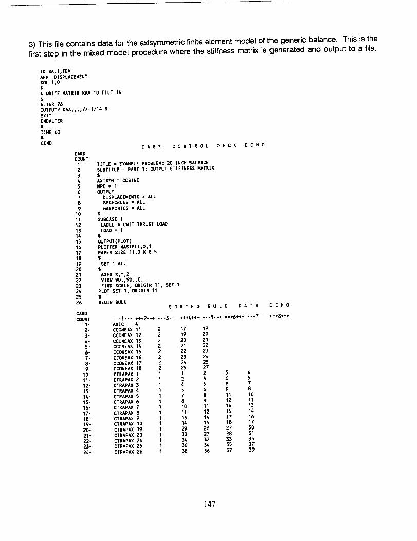
3) This file contains data for the axisymmetric finite element model of the generic balance. This is the
first step in the mixed model procedure where the stiffness matrix is generated and output to a file.
ID BALl,FENAPP DISPLACEMENT
SOL 1,0$$ WRITE MATRIX IOI,A TO FILE 14$ALTER 76
OUTPUT2 KAA.... 11-1114 $EXITENDALTER$TIME 60$
CEND
CARDCOUNT
12
3456789
1011121514151617
181920212223242526
CARDCOUNT
1-2-3-
4-5-
6-7-8"9-
10-11-12-13-14-
15-16-17-1B-19-20-
21-22-23-24-
CASE CONTROL DECK ECHO
TITLE = EXAMPLE PROBLEM: 20 INCH BALANCESUBTITLE = PART 1: OUTPUT STIFFNESS MATRIX
$AXISYM = COSINEMPC = 1OUTPUT
DISPLACEMENTS = ALLBPCFORCES = ALLHARMONICS = ALL
$SUBCASE 1
LABEL = UNIT THRUST LOAD
LOAD = 1$
OUTPUT(PLOT )PLOTTER NASTPLT,D, 1PAPER SIZE 11.0 X 8.5$
SET 1 ALL$
AXES X,Y,ZVIEW 90.,90.,0.FIND SCALE, ORIGIN 11, SET 1
PLOT SET 1, ORIGIN 11$
BEGIN BULKSORTED
""1"'" +++2+++ ""3"-- +++4+÷+AXIC 4CCONEAX 11 2 17CCONEAX 12 2 19
CCONEAX 13 2 20CCONEAX 14 Z 21CCONEAX 15 2 22CCONEAX 16 2 23CCONEAX 17 2 24CCONEAX 18 2 25CTRAPAX I I ICTRAPAX 2 I 2
CTRAPAX 3 I 4CTRAPAX 4 I 5
CTRAPAX 5 I 7CTRAPAX 6 1 8CTRAPAX 7 I 10
CTRAPAX 8 I 11
CTRAPAX 9 I 13
CTRAPAX 10 I 14
CTRAPAX 19 I
CTRAPAX 20 I 30
CTRAPAX 24 1 _4CTRAPAX 25 I
CTRAPAX 26 1 38
BULK DATA ECHO
"--5"-" +++6+*+ "'-7--- +++8+++
19
202122252425
272 5 43 6 5
5 8 76 9 88 11 109 12 1111 14 1312 15 1414 17 1615 18 17
26 27 3027 28 3132 33 3534 35 3736 37 39
147
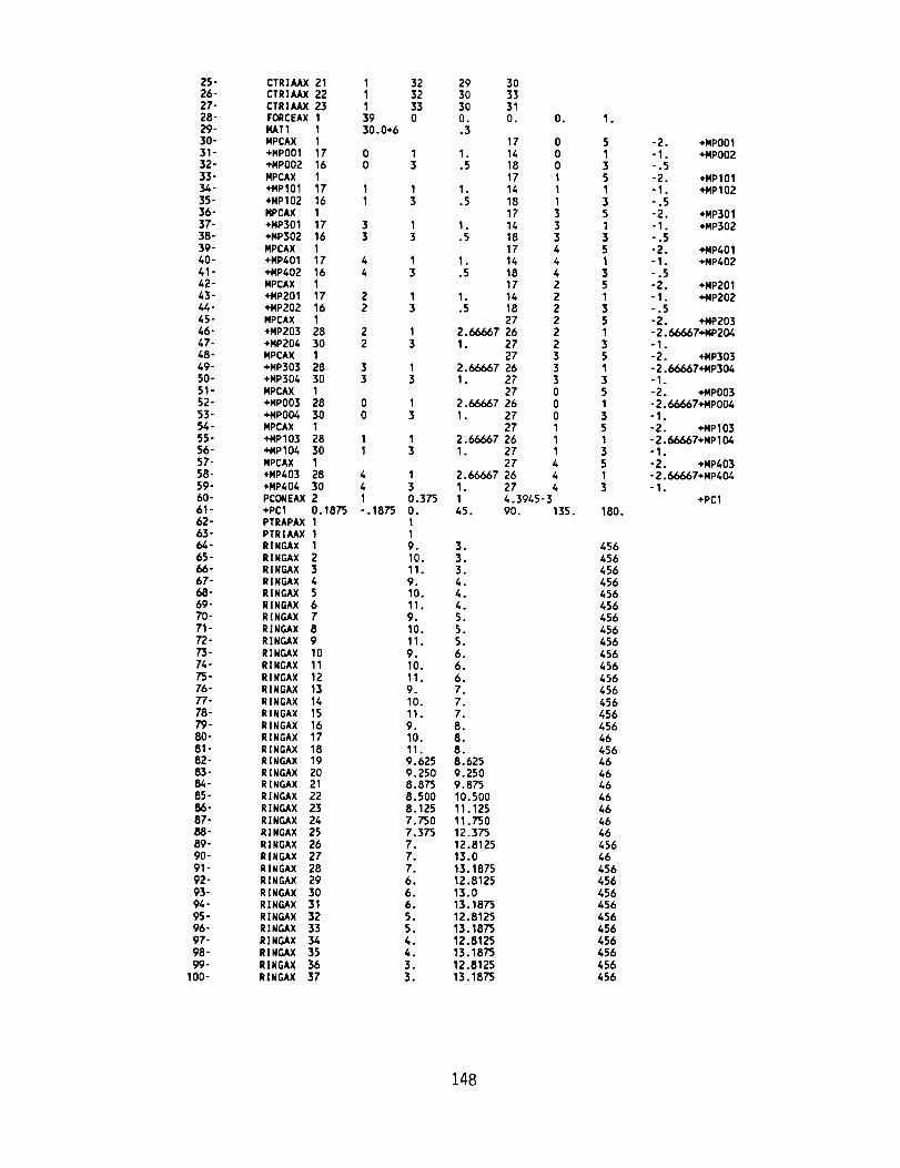
25-26-27-28-29-30-
31-32-33-34-35-36-37-38-39-40-41-42-
43-44-45-
46-47-48-
49-50-51-52-53-54-55-56-57-58-59-60-
61-62-63-64-65-66-67-68-69-70-71-72-73-74-
75-76-77-78-79-80-
81-82-83-84-85-
86-87-8a-89-90-91-
92-93-94-95-96-
97-98-99-
100-
CTRIAAX 21CTR]AAX 22CTRIAAX 23FORCEAX 1MAT1 1MPCAX 1+MPO01 17+MPO02 16
MPCAX 1+MPI01 17+MPI02 16NPCAX 1+MP301 17+MP302 16
MPCAX 1H,IP401 17+MP402 16MPCAX 1+MP201 17+MP202 16
MPCAX 1+MP203 28+MP204 30MPCAX 1+MP303 28+MP304 30MPCAX 1+MPO03 28÷MPO04 30MPCAX 1
+MPI03 28+MPI04 30
MPCAX 1+MP403 28+MP404 30PCONEAX 2+PC1 0.187'5PTRAPAX 1PTRIAAX 1RINGAX 1RINGAX 2RINGAX 3R] NGAX 4R]NGAX 5
RINGAX 6
RINGAX 7
RINGAX 8
RINGAX 9
RINGAX 10
RINGAX 11
R]NGAX 12
R]NGAX 13
R]NGAX 14
R]NGAX 15
R]NGAX 16
R|NGAX 17
RINGAX 18
RINGAX 19
RINGAX 20
R|NGAX 21
R[NGAX 22
R]NGAX 23
R]NGAX 24RINGAX 25
R%NGAX 26R]NGAX 27
R]NGAX 28RINGAX 29RINGAX 30RINGAX 31RINGAX 32RINGAX 33
R%NGAX 34RINGAX 35R]NGAX 36RINGAX 37
1 32 29 301 32 30 331 33 30 3139 0 O. O.30.0+6 .3
441- .1875
O.
3,
3.
3.4.4.
4.5.
5.5.6.6.
6.7.7.7.8.8.8.8.6259.2509.87510.500
11.125
11.750
12.375
12.812513.013.187512.812513.013.1875
12.812513.1875
12.812513.187512.812513.1875
17 01 1. 14 03 .5 18 0
17 11 1. 14 1
3 .5 18 117 3
1 1. 14 33 .5 18 3
17 41 1. 14 43 .5 18 4
17 21 1. 14 23 .5 18 2
27 2I 2.66667 26 23 1. 27 2
27 3
1 2.66667 26 33 1. 27 3
27 01 2.66667 26 03 1. 27 0
27 11 2.66667 26 13 1. 27 1
27 4I 2.66667 26 4
3 1. 27 40.375 1 4.3945-3O. 45. 90. 135.
I
I
9.
10.
11.
9.
10.
11.9.
10.
11.
9.
10.
11.9.
10.
11.
9.
10.
11.
9.625
9.250
8.8758.5008.1257.7507.375
7.7.7.6.6.6.
5.5.
4.4.3.
3.
1.
180.
456456456456456456456456456456
456456456456456456
46456464646
4646464645646456456456
456456456456456456456
-2. +MPO01-1. +MPO02".5
-2. ÷MPI01-1. +MPI02".5
-2. +MP301
-1. +MP302",5
-2. ÷MP401
"1. +MP402".5
-2. +MP201-1. +MP202".5
-2. +MP203-2.66667+MP204"1.
-2. +MP303-2.66667+MP304-1.
-2. +MPO03-2.66667+MP004"1.
-2. _P103-2.66667+MP104"1.
-2. +MP403-2.66667+MP404
-1.
+PC1
148
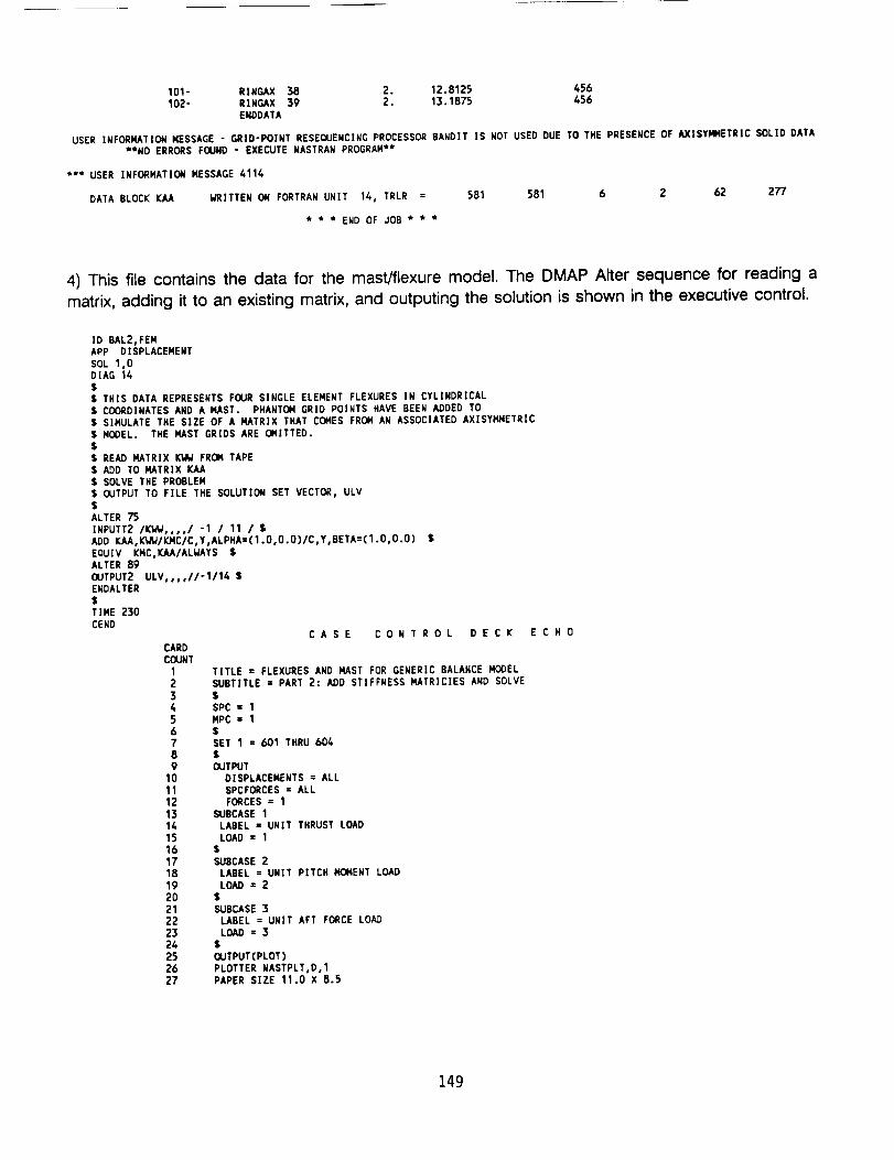
101- RINGAX 38 2. 12.8125 456102- RINGAX 39 2. 13.1875 456
ENDDATA
USER INFORMATION MESSAGE " GRID'POINT RESEQUENCING PROCESSOR BANDIT IS NOT USED DUE TO THE PRESENCE OF AXISYMMETRIC SOLID DATA
**NO ERRORS FOUND " EXECUTE NASTRAN PROGRAM**
*** USER INFORMATION MESSAGE 4114
DATA BLOCK ICAA MRITTEN ON FORTRAN UNIT 14, TRLR = 581 581 6 2 62 277
* *' * END OF JOB * * *
4) This file contains the data for the mast/flexure model. The DMAP Alter sequence for reading a
matrix, adding it to an existing matrix, and outputing the solution is shown in the executive control.
ID BAL2,FEMAPP DISPLACEMENT
SOL 1,0DIAG 14S$ THIS DATA REPRESENTS FOUR SINGLE ELEMENT FLEXURES IN CYLINDRICAL$ COORDINATES AND A MAST. PHANTOM GRID POINTS HAVE BEEN ADDED TO$ SIMULATE THE SIZE OF A HATRIX THAT COMES FROH AN ASSOCIATED AXISYMHETRIC
$ MODEL. THE HAST GRIDS ARE OMITTED.$$ READ MATRIX _ FROM TAPE$ ADD TO MATRIX KAA$ SOLVE THE PROBLEM$ OUTPUT TO FILE THE SOLUTION SET VECTOR, ULV$ALTER 7'5
INPUTT2 /Kt,N .... / -1 / 11 / $ADD KAA,IO,I_/KMC/C,Y,ALPHA=(1.0,O.O)/C,Y,BETA=(1.0,O.O) $EQUIV KNC.IO_A/ALWAYS $ALTER 89OUTPUT2 ULV .... //-1/14 $ENDALTER$TIME 230CEND
CASE CONTROL DECK ECHO
CARDCOUNT
1 TITLE : FLEXURES AND HAST FOR GENERIC BALANCE MODEL2 SUBTITLE = PART 2: ADD STIFFNESS MATRICIES AND SOLVE
3 $4 SPC = 15 HPC = 16 $7 SET 1 : 601 THRU 6048 $9 OUTPUT
10 DISPLACEMENTS : ALL11 SPCFORCES = ALL
12 FORCES = I13 SUBCASE 114 LABEL = UNIT THRUST LOAD15 LOAD = 116 $17 SUBCASE 218 LABEL = UNIT PITCH MOMENT LOAD19 LOAD = 2
2O $21 SUBCASE 322 LABEL : UNIT AFT FORCE LOAD
23 LOAD : 324 $25 OUTPUT(PLOT)26 PLOTTER NASTPLT,D,127 PAPER SIZE 11.0 X 8.5
149
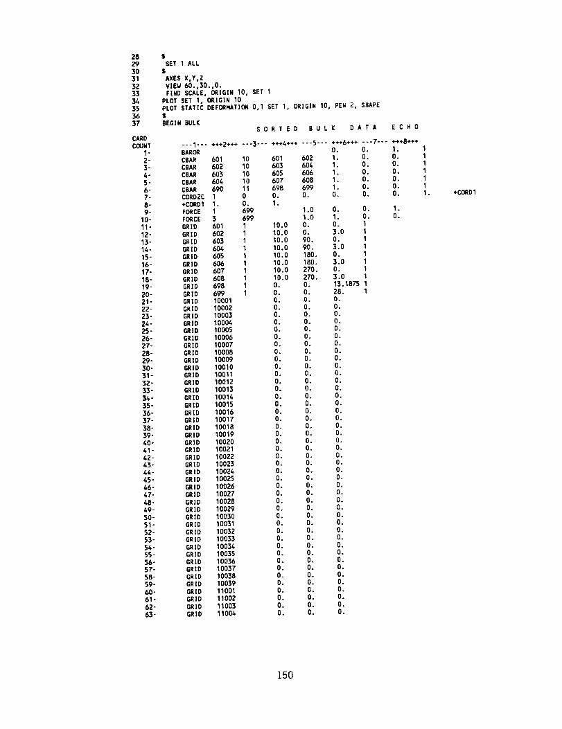
28293O313233
34353637
$SET 1 ALL
S
AXES X,Y,ZVIEW 60.,30.,0.FiND SCALE, ORIGIN 10, SET 1
PLOT SET 1, ORIGIN 10PLOT STATIC DEFORHATION 0,1 SET 1, ORIGIN 10, PEN 2, SHAPE$BEGIN BULK
SORTED BULK DATA ECHO
CARDCOUNT ---1--- +++2+++ ---3--- +++4+++ ---5--- +++6+++ ---7--- +++8+++
1- BAROR O. O. 1. 12- CBAR 601 10 601 602 1. O. O. 13- CBAR 602 10 603 604 1. O. O. 16- CBAR 603 10 605 606 1. O. O. 15" CBAR 604 10 607 608 1. O. O. 16" CBAR 690 11 698 699 1. O. O. 17" CORD2C 1 0 O. O. O. O. O. 1.8- +CORD1 1. O. 1.9- FORCE 1 699 1.0 O. O. 1.
10- FORCE 3 699 1.0 1. O. O.
11- GRID 601 1 10.0 O. O. 112- GRID 602 1 10.0 O. 3.0 113- GRID 603 1 10.0 90. O. 114 ° GRID 604 1 10.0 90. 3.0 115" GRID 605 1 10.0 160. O. 116- GRID 606 1 10.0 180. 3.0 117- GRIO 607 1 10.0 270. O. 118- GRID 608 1 10.0 270. 3.0 119- GRID 698 1 O. O. 13.1875 1
20" GRID 699 1 O. O. 28. 121" GRID 10001 O. O. O.
22" GRID 10002 O. O. O.23" GRiD 10003 O. O. O.24- GRID 10004 O. O. O.25- GRID 10005 O. O. O.
26- GRID 10006 O. O. O.27- GRID 10007 O. O. O.
28- GRID 10008 O. 0. O.
29- GRiD 10009 O. O. O.
30- GRID 10010 O. O. O.
31- GRiD 10011 O. O. O.
32- GRID 10012 O. O. O.33- GRID 10013 O. O. O.34- GRiD 10014 O. O. O.35- GRID 10015 O. O. O.
36- GRID 10016 O. O. O.
37- GRID 10017 O. O. O.38- GRID 10018 O. O. O.39- GRID 10019 O. 0. O.
40- GRID 10020 O. O. O.
41- GRID 10021 O. O. O.42- GRiD 10022 O. O. O.43- GRID 10023 O. O. O.44- GRID 10024 O. O. O.45- GRID 10025 O. O. O.46- GRID 10026 O. O. O.
47- GRID 10027 O. O. O.
48- GRID 10028 O. O. O.
49- GRID 10029 O. O. O.50- GRID 10030 O. O. D.51- GRID 10031 O. O. O.
52" GRID 10032 O. O. O.53- GRID 10033 O. O. O.54- GRID 10034 O. O. O.55- GRiD 10035 O. O. O.56- GR%D 10036 O. O. O.
57- GRID 10037 O. O. O.58- GRID 10038 0. O. O.59" GRID 10039 O. O. 0.
00- GRID 11001 O. O. O.
61- GRID 11002 O. O. O.
62- GRID 11003 O. O. O.63- GRID 11004 O. O. O.
+CORD1
150
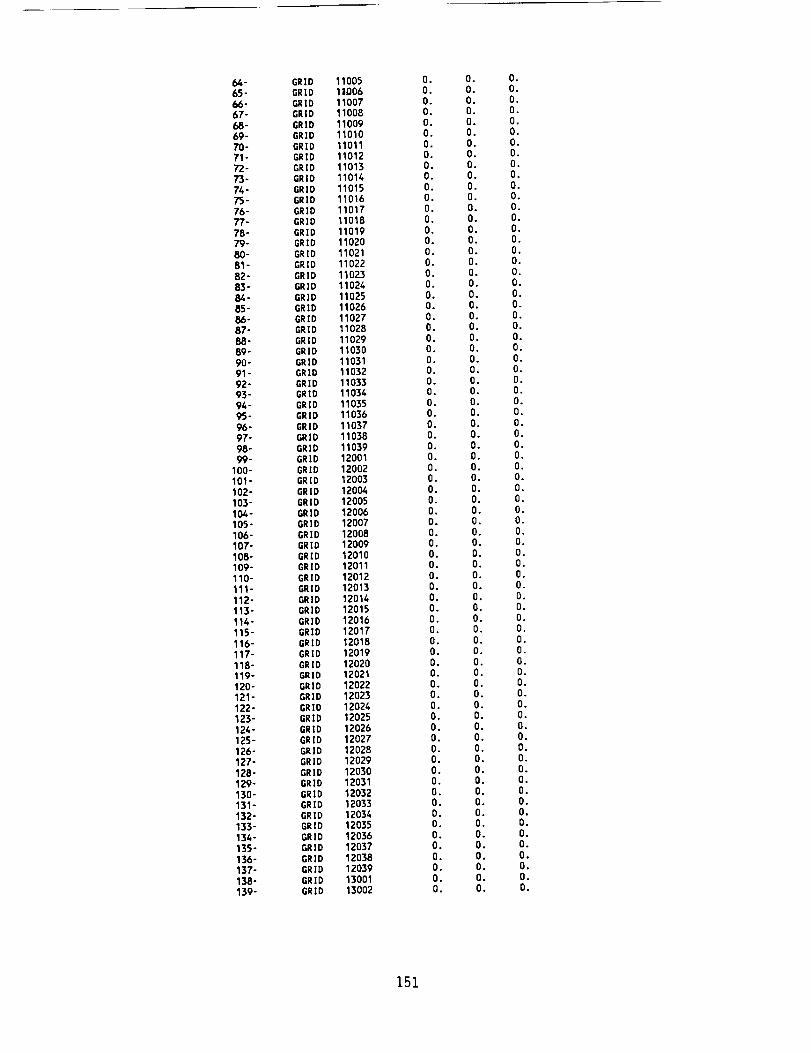
65"
66"67"68"69"70"71"72"73"74"75"76"77"78-
79"80-81"82"83"84"85-
86"87"88"89"90"91"92"93"94"95"
96"97"
98"99"
100-101 -102-103-
104-105-
I06-
107-108-
109-
110-
111-
112-
113-
114-
115-
116-
117-
118"119-
120-
121 -
122-123-124-125-126"
127-
128-
129-130-
131-
132-133-134-135-136-
137-138-139-
GRIDGRIDGRIDGRiDGRIDGRIDGRIDGRIDGRIDGRiD
GRIDGRIDGRID
GRID
GRID
GRIDGRIDGRID
GRIDGRID
GRIDGRIDGRIDGRIDGRiDGRID
GRIDGRID
GRIDGRIDGRIDGRIDGRiDGRIDGRIDGRID
GRIDGRIDGRIDGRIDGRIDGRIDGRIDGRIDGRIDGRiD
GRIDGRIDGRIDGRIDGRIDGRID
GRIDGRIDGRiDGRIDGRIDGRIDGRIDGRID
GRIDGRID
GRIDGRIDGRIDGRIDGRIDGRIDGRIDGRIDGRID
GRIDGRIDGRIDGRIDGRID
11005
I1006
11007
11008
11009
11010
11011
11012
11013
11014
11015
11016
11017
11018
11019
11020
11021
11022
11023
11024
11025
11026
11027
11028
1102911030
11031
11032
11033
11034
11035
11036
11037
11038
11039
12001
12002
12003
120041200512006
12007
120081200912010120111201212013120141201512016
12017120181201912020120211202212023
1202412025
120261202712028120291203012031
1203212033
120341203512036120371203812039
1300113002
O,
O.O.O.O.O.O.O.O.O.
O.O.O.O.O.O.O.O.
O.O.O.O.O.O.O.O.
O.O.O.O.O.O.O.O.O.O.
O.O.O.O.O.O.O.O.
O.O.O.O.O.O.
O.O.O.O.O.O.O.O.
O.O.
O.O.O.O.O.O.
O.O.O.O.
O.O.O.O.O.O.
Oo
O.
O.O.
O.O.O.O.O.O.O.O.O.O.O.O.
O.O.O.O.O.O.
O.O.
O.O.O.O.O.O.O.O.O.
O.O.O.O.O.O.
O.O.O.O.O.O.O.O.O.
O.O.O.O.O.
O.O.O.O.O.O.O.O.O.O.O.
O.O.O.O.O.O.O.O.
O.O.O.O.
Oo
O.
O.
O.
O.
O.
O.
O.
O.
O.
O.
O.
O.
O.
O.
O.
O.
O.
O.
O.
O.
O.
O.
O.
O.
O.
O.
O.
O.O.
O.
O.
O.
O.
O.
O.
O.O.
O.
O.
O.
O.
O.
O.
O.
O.
O.
O.
O.
O.
O.
O.
O.
O.
O.
O.
O.
O.
O.
O.
O.
O.
O.
O.
O.
O.
O.
O.
O.
O.
O.O.
O.
O.
O.
O.
151
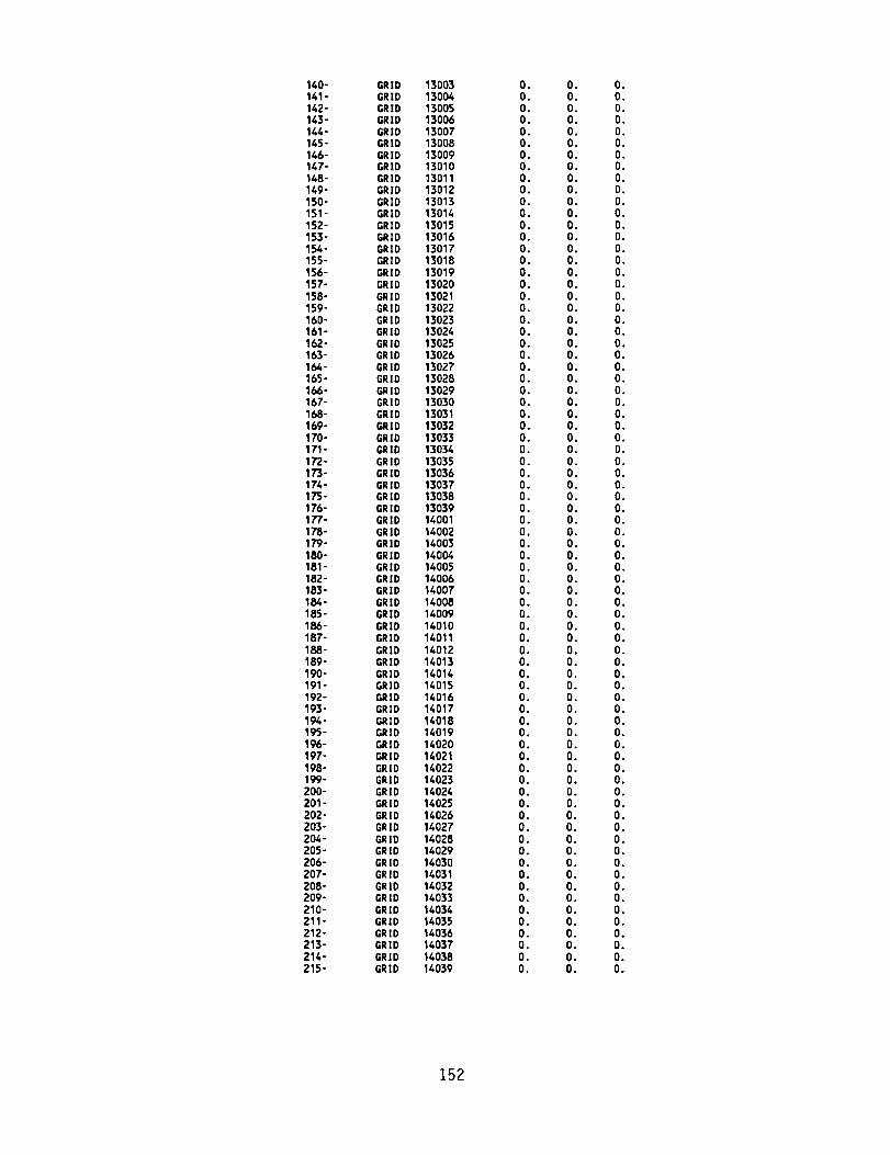
140"141"
142-143-144-145-146-147-148-149-150-
151 -152-153-154-155-156-157-158-159-
160-161 -
162-163-164-165-166-167-168-169-170-171 -
172-173-174-175-176"177"
178"179"180"181 "182"183-184-185-186-187-
188-189-190-191-192-193-194-195-196-197-198-199-
200-201 -202-203-204-205-
206 -207 -
208-209 -210-211-212-213-214-215-
GRiDGRID
GRIDGRID
GRIDGRiDGRIDGRID
GRIDGRID
GRiDGRIDGRIDGRIDGRIDGRiDGRIDGRID
GRIDGRIDGRiDGRIDGRIDGRIDGRIDGRIDGRIDGRIDGRIDGRiDGRID
GRIDGRIDGRIDGRIDGRIDGRIDGRIDGRIDGRIDGRiDGRIDGRIDGRiDGRiDGRID
GRIDGRIDGRIDGRIDGRIDGRIDGRIDGRID
GRIDGRID
GRiDGRIDGRIDGRIDGRIDGRIDGRIDGRID
GRIDGRIDGRIDGRIDGRIDGRIDGRIDGRIDGRIDGRIDGRIDGRID
1300313004
130051300613007130081300913010130111301213O13130141301513016
130171301813019130201302113022
1302313024
130251302613027130281302913030130311303213033130341303513036
1303713038
1303914001
1400214003140041400514O061400714008140091401014011
140121401314014140151401614017140181401914020
140211402214023140241402514026140271402814029
1403014031
1403214033140341403514036140371403814039
O,
O.O.O.O.O.O.O.O.O.O.O.O.O.
O.O.
O.O.O.O.O.O.O.O.
O.O.O.O.O.O.O.O.O.O.
O.O.O.O.
O.O.O.O.O.O.O.O.O.O.
O.O.O.O.O.O.O.O.O.
O.O.O.O.O.O.O.O.O.
O.O.
O,O.O.O.O.O.O.O.
O,
O.O.O.O.O.O.O.O.O.O.O.O.O.
O.O.
O.O.O.O.O.O.O.O.O.O.
O.O.O.O.O.O.O.O.
O.O.O.O.
O.O.O.O.O.O.O.O.O.O.
O.O.O.O.O.O.O.O.O.O.
O.O.O.O.O.O.O.O.
O.O.
O.O.O.O.O.O.O.O.
Oo
O.O.O.O.O.O.O.O.O.O.O.O.O.O.O.
O.O.O.O.O.O.O.O.O.O.
O.O.O.O.O.O.O.O.
O.O.O.O.
O.O.O.O.O.O.O.O.O.O.
O.O.O.O.O.O.O.O.O.
O.O.O.O,O.O.O.O.O.
O.O.
O.O.O.O.O.O.O.O.
152
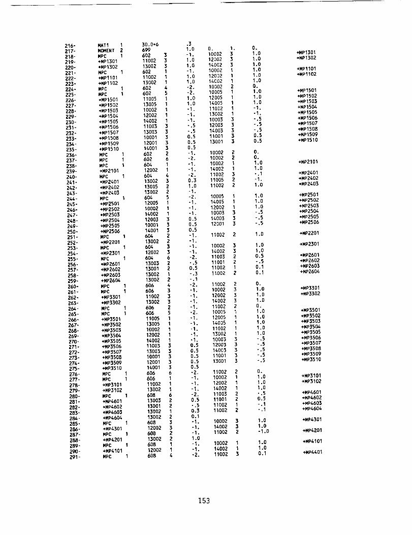
216"217"218"219-220"221"
222"223-
224"225"226-227-228-229-230-231-
232-233 -234 -235 -236 -237-238 -239 -240-241-
242 -243-
244-
245-
246 -
247-
248-249-
250-
251 -
252-253-
254-
255-
256-257-258-259-260 -261 -
262 -263 -264-265 -266-
267 -268-269-270-271 -2T2-273-274 -27'5-276-277-
278-279-280-281 -282-283-
284-285 -286-
287"288"289 -
290 -
291 -
MATI I
MOMENT 2
MPC I
+MP1301
+MP1302
MPC I
+MP1101
+MP1102
MPC 1MPC I
+MP1501
+MP1502
+MP1503
÷MP1504
+MP1505
÷MP1506
÷MP150T
÷MP1508
÷MP1509
+MP1510
MPC I
MPC I
MPC I
÷MP2101
MPC I
÷MP2401
+MP2402
÷MP2403
MPC I
÷MP2501
+MP2502
+MP2503
+MP2504
÷MP2505
÷MP2506
MPC I
+MP2201
MPC I
+MP2301
MPC I
+MP2601
+MP2602
+MP2603
+MP26O4
MPC I
MPC I
+MP3301÷MP3302
MPC I
MPC I
÷MP3501
÷MP3502
+MP3503
+MP3504
+MP3505
+MP3506
+MP3507
+MP3508
÷MP3509
÷MP3510
MPC I
MPC I
÷MP3101
÷MP3102
MPC I
+MP4601
+MP4602
÷MP4603+MP4604
MPC I+MP4301
MPC I
+MP4201
MPC I
÷MP4101
MPC I
30.0+6
699
602
11002
13002
602
11002
13002
602
602
11005
13005
10002
12002
14002
11003
1300310001
12001
14001
602
602
604
12002
604
13002
13005
13002
604
12005
10002
14002
12003
10001
14001
6O4
13002
604
12002
604
13003130011300213002
606606
1100213002606606
110051300510002
12002
14002
11003
13003
10001
12001
14001
606
606
11002
13002
608
13003130011300213002608
12002
608
13002
608
12002
608
33
3111451111
1333332611
43225111
333223362
212433
325111
11333336111
62
21233221
14
.31.0 O. 1. O.-1. 10002 3 1.01.0 12002 3 1.0
1.0 14002 3 1.0-1. 10002 1 1,01.0 12002 1 1.01.0 14002 1 1.0-2. 10002 2 O.
-2. 10005 I 1.0
1.0 12005 I 1.0
1.0 14005 I 1.0
-I. 11002 I -I.
-I. 13002 I -I.
-I. 10003 3 -.5
-.5 12003 3 -.5
-.5 14003 3 -.5
0.5 11001 3 0.50.5 13001 3 0.5
0,5-I. 10002 2 O.
-2. 10002 2 O.
-I. 10002 I 1.0
-I. 14002 I 1.0
-2. 11002 3 -.I
0.3 11005 2 -I.
1.0 11002 2 1.0
"I.
-2. 10005 I 1.0
-I. 14005 I 1.0
-I. 12002 I 1.0
-I. 10003 3 -.5
0.5 14003 3 -.5
0.5 12001 3 -.5
0.5
-I. 11002 2 1.0
"I.
-I. 10002 3 1.0
"I. 14002 3 1.0
-2. 11003 2 0.5
-.5 11001 2 -.5
0.5 11002 I 0.1
-.3 11002 2 0.1
°.I
-2. 11002 2 O.
"I. 10002 3 1.0
-I. 12002 3 1.0
-I, 14002 3 1.0
-I. 11002 2 O.
-2. 10005 I 1.0
-I. 12005 I 1.0
-I. 14005 I 1.0
-1. 11002 1 1.0-1. 13002 1 1.0-1. 10003 3 -.5
0.5 12003 3 -.5
0.5 14003 3 -,50.5 11001 3 -.5
0.5 13001 3 -.5
0.5
-2. 11002 2 O.
-I. 10002 I 1.0
-I. 12002 I 1.0
-I. 14002 I 1.0
-2. 11003 2 -.5
0.5 11001 2 0.5
-.5 11002 I -.I
0.3 11002 2 -.I
0.1
-1. 10002 3 1.0-1. 14002 3 1.0-1. 11002 2 -1.0
1.0-1. 10002 1 1.0-1. 14002 1 1.0
-2. 11002 3 0.1
÷MP1301
+MP1302
+MP1101
÷MP1102
+MP1501
÷MP1502
+MP1503
+MP1504
+MP1505
÷MP1506
+MP1507
+MP1508
÷MP1509
+MP1510
+MP2101
÷MP2401
÷MP2402
*MP2403
÷MP2501
÷MP2502
+MP2503
+MP2504
÷MP2505
+MP2506
÷MP2201
÷MP2301
+MP2601
+MP2602
+MP2603
÷MP2604
+MP3301
+MP3302
+MP3501
÷MP3502
+MP3503
÷MP3504
÷MP3505
+MP3506
÷MP3507
÷MP3508
+MP3509
÷MP3510
+MP3101
+MP3102
÷MP4601
÷MP4602
+MP4603
+MP4604
+MP4301
+MP4201
+MP4101
+MP4401
153
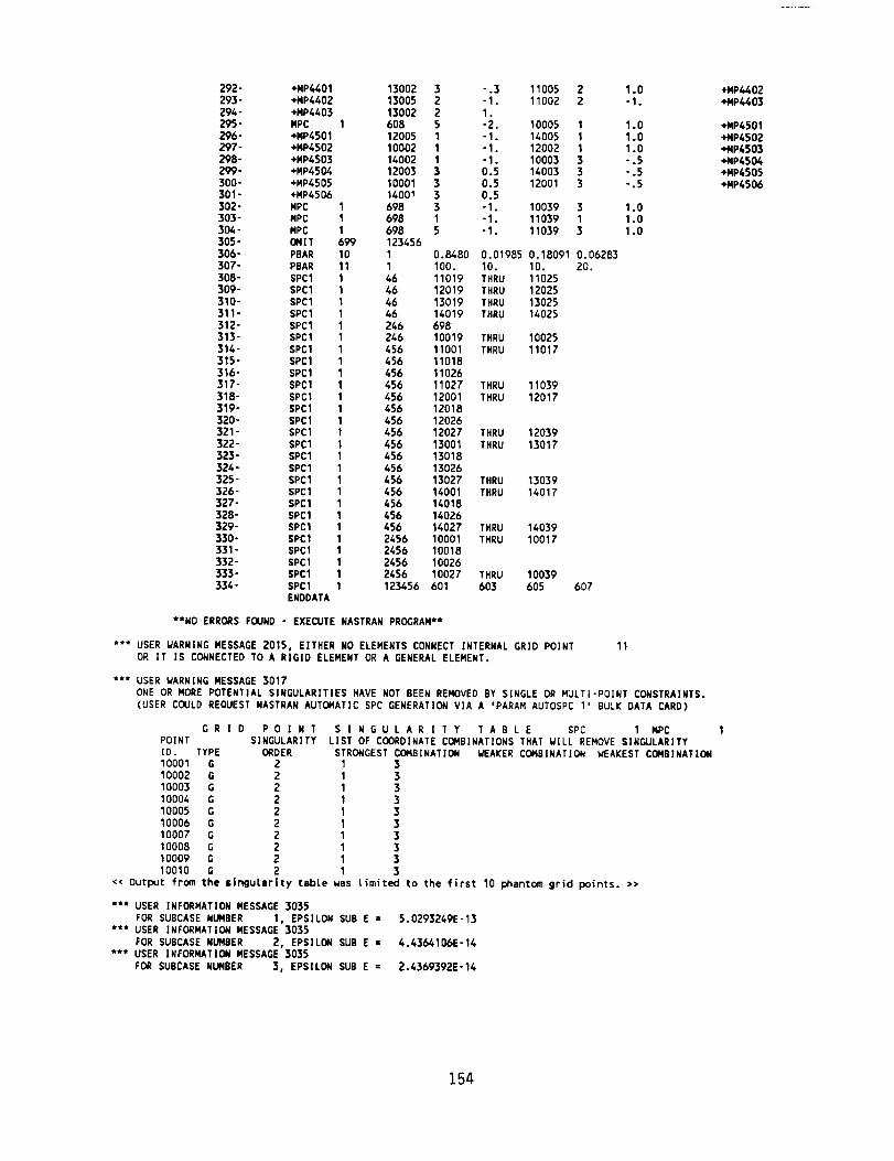
292- +NP4401 13002 3 -.3 11005 2293- +NP4402 13005 2 -1. 11002 2294- +NP4403 13002 2 1.295- NPC 1 608 5 -2. 10005 1296- ÷NP4501 12005 1 -1. 14005 1297- ÷NP4502 10002 1 -1. 12002 1298- ÷NP4503 14002 1 -1. 10003 3299- ÷NP4504 12003 3 0.5 14003 3300- ÷NP4505 10001 3 0.5 12001 3301- +NP4506 14001 3 0.5302- NPC 1 698 3 -1. 10039 3303- NPC 1 698 1 -1. 11039 1304- NPC 1 698 5 -1. 11039 3305- OMIT 699 123456
306- PBAR 10 1 0.6480 0.01985 0.18091 0.06283307- PBAR 11 1 100. 10. 10. 20.308- SPCl 1 46 11019 THRU 11025309- SPCl 1 46 12019 THRU 12025310- SPCl 1 46 13019 THRU 13025311- SPC1 1 46 14019 THRU 14025312- SPCl 1 246 698313- SPCl 1 246 10019 THRU 10025314- SPCl 1 456 11001 THRU 11017315- SPCl 1 456 11018
316- SPCl I 456 11026317- SPCl 1 456 11027 THRU 11039318- SPCl 1 456 12001 THRU 12017319- SPCl 1 456 12018320- SPC1 1 456 12026321- SPCl 1 456 12027 THRU 12039322- SPCl 1 456 13001 THRU 13017323- SPCl 1 456 13018324- SPC1 1 456 13026
325- SPCl 1 456 13027 THRU 13039326- SPCl 1 456 14001 THRU 14017327- SPCl 1 456 14018328- SPCl 1 456 14026329- SPCl 1 456 14027 THRU 14039330- SPCl 1 2456 10001 THRU 10017331- SPC1 1 2456 10018332- SPCl 1 2456 10026333- SPC1 1 2456 10027 THRU 10039334- SPCl 1 123456 601 603 605 607
ENDDATA
**NO ERRORS FOUND - EXECUTE NASTRAN PROGRAM**
*** USER WARNING MESSAGE 2015, EITHER NO ELEMENTS CONNECT INTERNAL GRID POINTOR IT IS CONNECTED TO A RIGID ELEMENT OR A GENERAL ELEMENT.
1.0"1o
1.0
1.01.0°.5
".5
".5
1.01.0
1.0
11
*** USER WARNING MESSAGE 3017
ONE OR MORE POTENTIAL SINGULAR|TIES HAVE NOT BEEN REMOVED BY SINGLE OR MULTI-POINT CONSTRAINTS.
(USER COULD REQUEST NASTRAN AUTOMATIC SPC GENERATION VIA A 'PARAM AUTOSPC 1 _ BULK DATA CARD)
GRID POINTPO]NT S ] NGULARI TY[D. TYPE ORDER10001 G 2 1 310002 G 2 1 310003 G 2 1 3
10004 G 2 I 310005 G 2 1 310006 G 2 1 310007 G 2 1 310008 G 2 1 310009 G 2 1 310010 G 2 1 3
SINGULARITY TABLE SPC 1 NPCLIST OF COORDINATE COMBINATIONS THAT WILL REMOVE SINGULARITY
STRONGEST COL_4BINATION WEAKER COMBINATION WEAKEST CONBINATION
<< Output from the singularity table aas Limited to the first 10 phantom grid points. >>
*** USER INFORMATION NESSAGE 3035
FOR SUBCASE NLINBER 1, EPSILON SUB E = 5.0293249E-13*** USER INFORMATION NESSAGE 3035
FOR SUBCASE NUMBER 2, EPSILON SUB E = 4.4364106E-14*** USER INFORMATION MESSAGE 3035
FOR SUBCASE NUMBER 3, EPSILON SUB E = 2.4369392E'14
÷NP44024-NP4403
÷NP4501+NP4502+NP4503+NP4504+NP4505+NP4506
154
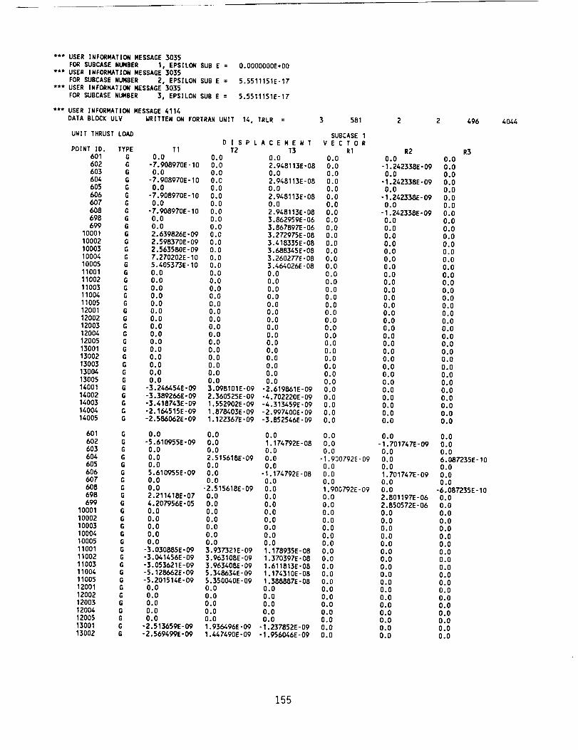
*** USER INFORI4ATION MESSAGE 3035FOR SUBCASE NUMBER 1, EPSILON SUB E =
*** USER INFORMATION MESSAGE 3035FOR SUBCASE NUNBER 2, EPSILON SUB E =
*** USER INFORMATION MESSAGE 3035FOR SUBCASE NUMBER 5, EPSILON SUB E =
0.O000000E+O0
5.5511151E'17
5.5511151E-17
*** USER INFORMATION MESSAGE 4114DATA BLOCK ULV WRITTEN ON FORTRAN UNIT 14, TRLR = 3 581 2 2
UNIT THRUST LOAD SUBCASE 1D | SPLACEMENT VECTOR
POINT ID. TYPE T1 T2 T3 R1 R2 R3601 G 0.0 0.0 0,0 0.0 0.0 0.0
602 G -7.908970E- 10 0.0 2.948113E-06 0.0 - 1.242338E-09 0.0603 G 0.0 0.0 0.0 0.0 0.0 0.0
604 G -7.908970E- 10 0.0 2.948113E-08 0.0 - 1.242338E-09 0.0605 G 0.0 0.0 0.0 0.0 0.0 0.0606 G -7.908970E- I0 0.0 2.948113E-08 0.0 - 1.242338E-09 0.0607 G 0.0 0.0 0.0 0.0 0.0 0.0
608 G -7.908970E- I0 0.0 2.948113E-08 0.0 -I .242338E-09 0.0698 G 0.0 0.0 3.862959E- 06 0.0 0.0 0.0
699 G 0.0 0.0 3.867897E-06 0.0 0.0 0.010001 G 2.639826E- 09 0,0 3. 272975E- 08 0.0 0.0 0.010002 G 2.598370E-09 0.0 3.418335E-08 0.0 0.0 0.010003 G 2.563580E-09 0.0 3.688545E-08 0.0 0.0 0.010004 G 7.270202E- 10 O. 0 3.260277E- 08 O. 0 O. 0 O. 010005 G 5.405373E- 10 0.0 3.464026E-08 0,0 0.0 0.0
11001 G 0.0 0.0 0.0 0.0 0,0 0.011002 G 0.0 0.0 0.0 0.0 0.0 0.011003 G 0.0 0.0 0.0 0.0 0.0 0.011004 G 0.0 0.0 0.0 0.0 0.0 0.011005 G 0.0 0.0 0.0 0.0 0.0 0.012001 G 0.0 0.0 0.0 0.0 0.0 0.012002 G 0.0 0.0 0.0 0.0 0.0 0.012003 G 0.0 0.0 0.0 0.0 0.0 0.012004 G 0.0 0.0 0.0 0.0 0.0 0.0
12005 G 0.0 0.0 0.0 0.0 0.0 0.013001 G 0.0 0.0 0.0 0.0 0.0 0.013002 G 0.0 0.0 0,0 0.0 0.0 0.013003 G 0.0 0.0 0.0 0.0 0.0 0.013004 G 0.0 0.0 0.0 0.0 0.0 0.013005 G 0.0 0.0 0.0 0.0 0.0 0.014001 G -3.246454E-09 3.098101E-09 -2.619861E-09 0.0 0.0 0.014002 G -3.3892_E -09 2.360525E-09 -4.702220E-09 0.0 0.0 0.014003 G -3.418743E-09 1.552902E-09 -4.513459E-09 0.0 0.0 0.0
14004 G -2,164515E-09 1.878403E-09 -2.4;_7400E-09 0.0 0.0 0.014005 G -2.586062E-09 1.122367E-09 -3.B52546E-09 0.0 0.0 0.0
4_
601 G 0.0 0.0 0.0 0.0 0.0 0.0602 G -5.610955E-09 0.0 1. 174792E-08 0.0 - 1.701747E-09 0.0605 G 0.0 0.0 0.0 0.0 0.0 0.0604 G 0.0 2.515618E-09 0.0 -1,900792E-09 0.0 6.087235E- I0
605 G 0.0 0.0 0.0 0.0 0.0 0.0
606 G 5.610955E-09 0.0 - 1.174792E-08 0.0 1.701747E-09 0.0607 G 0.0 0.0 0.0 0.0 0.0 0.0
608 G 0.0 -2.515618E-09 0.0 1.900792E-09 0.0 -6.087235E- I0
698 G 2.211418E-07 0.0 0.0 0.0 2.801197E-06 0.0699 G 4.207956E-05 0.0 0.0 0.0 2.850572E-06 0.0
10001 G 0.0 0.0 0.0 0.0 0.0 0.010002 G 0.0 0.0 0.0 0.0 0.0 0.010003 G 0.0 0.0 0.0 0.0 0.0 0.0
10004 G 0.0 0.0 0,0 0,0 0.0 0.010005 G 0.0 0.0 0.0 0.0 0.0 0.0
11001 G -5.030885E-09 3.957321E-09 1.178735E-08 0.0 0.0 0.011002 G -3.041456E-09 3.963108E-09 1.370397E-08 0.0 0.0 0.011003 G -3.053621E-09 3.963408E- 09 1.611813E-08 0.0 0.0 0.011004 G -5.128_2E-09 5.548634E- 09 I. 174310E-08 0.0 0.0 0.011005 G -5.201514E-09 5.350040E- 09 1.388887E- 08 0.0 0.0 0.012001 G 0.0 0.0 0.0 0.0 0.0 0.012002 G 0.0 0.0 0.0 0.0 0.0 0.012003 G 0.0 0.0 0.0 0.0 0.0 0.0
12004 G 0,0 0,0 0.0 0.0 0.0 0.012005 G 0.0 0.0 0.0 0.0 0.0 0.015001 G -2.513659E-09 1.936496E-09 -1.237852E-09 0.0 0.0 0.013002 G -2.569499E-09 1.447490E-09 -1.956046E-09 0.0 0.0 0.0
4044
155
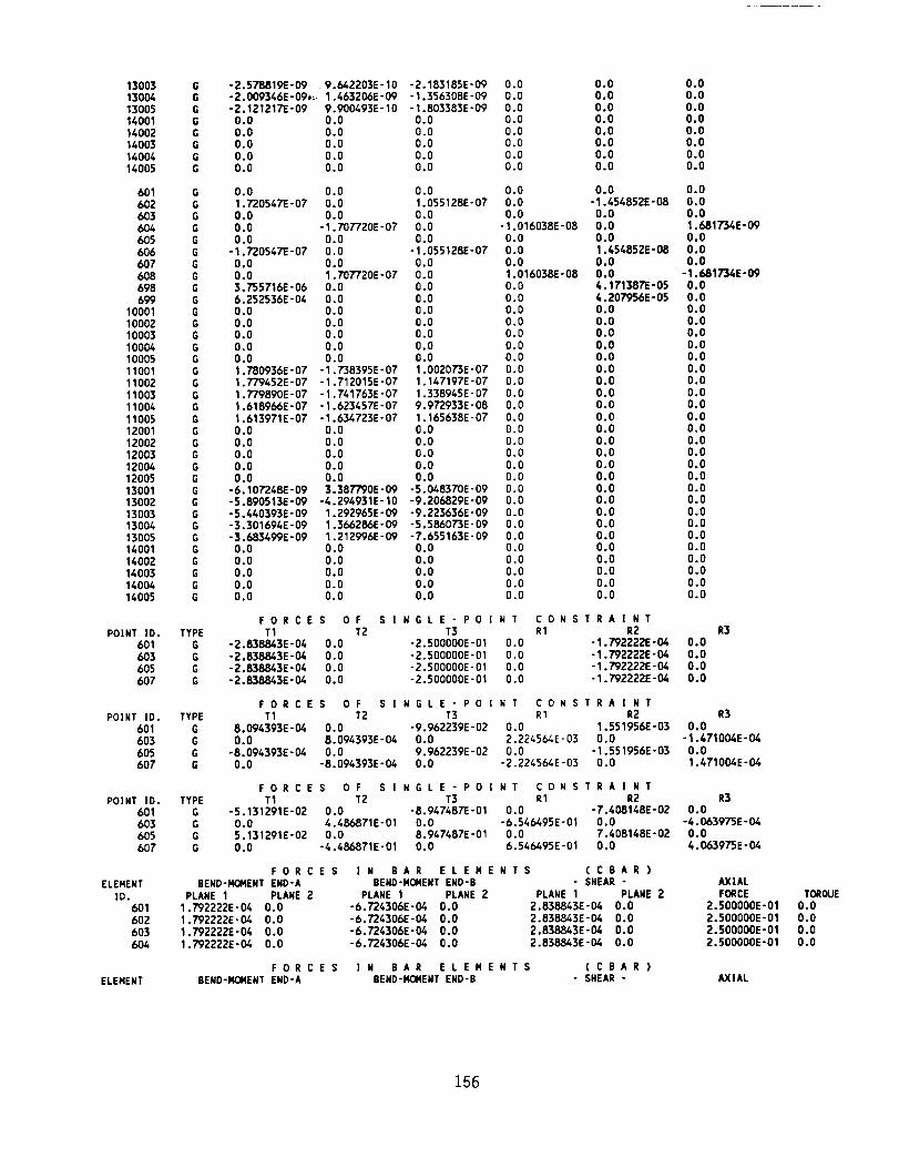
1300313004130051400114002140031400414005
G -2.578819E-09 9.642203E- 10 -2.183185E-09 0.0 0.0 0.0G -2.009346E-09,; 1.463206E-09 -1.356308E-09 0.0 0.0 0.0G -2.121217E-09 9.900493E- 10 - 1.803383E-09 0.0 0.0 0.0G 0.0 0.0 0.0 0.0 0.0 0.0
G 0.0 0.0 0.0 0.0 0.0 0.0
G 0.0 0.0 0.0 0.0 0.0 0.0G 0.0 0.0 0.0 0.0 0.0 0.0G 0.0 0.0 0.0 0.0 0.0 0.0
601 G 0.0 0.0 0.0 0.0 0.0 0.0602 G 1.720547E- 07 0.0 1 . 055128E- 07 0.0 -1.454852E-08 0.0603 G 0.0 0.0 0.0 0.0 0.0 0.0
604 G 0.0 -1 . 707720E- 07 0.0 -1. 016038E- 08 0.0 1.681734E- 09605 G 0.0 0.0 0.0 0.0 0.0 0.0
606 G -1.720547E-07 0.0 - 1.055128E-07 0.0 1.454852E-08 0.0607 G 0.0 0.0 0.0 0.0 0.0 0.0608 G 0.0 1 . 707720E- 07 0.0 1 . 016038E-08 0.0 -1.6817'34E- 09698 G 3.755716E-06 0.0 0.0 0.0 4.171387E-05 0.0699 G 6.252536E- 04 O. 0 O. 0 O. 0 4.207956E- 05 O. 0
10001 G 0.0 0.0 0.0 0.0 0.0 0.010002 G 0.0 0.0 0.0 0.0 0.0 0.010003 G 0.0 0.0 0.0 0.0 0.0 0.010004 G 0.0 0.0 0.0 0.0 0.0 0.010005 G 0.0 0.0 0.0 0.0 0.0 0.011001 G 1.780936E-07 -1.738395E-07 1.002073E-07 0.0 0.0 0.011002 G 1.779452E-07 -1.712015E-07 1.147197E-07 0.0 0.0 0.0
11003 G 1.779890E-07 -1.741763E-07 1.338945E-07 0.0 0.0 0.011004 G 1.618966E-07 -1.623457E-07 9.972933E-08 0.0 0.0 0.0
11005 G 1.613971E-07 - 1.634723E-07 1.165638E-07 0.0 0.0 0.012001 G 0.0 0.0 0.0 0.0 0.0 0.012002 G 0.0 0.0 0.0 0.0 0.0 0.012003 G 0.0 0.0 0.0 0.0 0,0 0.012004 6 0.0 0.0 0.0 0.0 0.0 0.012005 G 0.0 0.0 0.0 0.0 0.0 0.013001 G -6.107248E-09 3.387790E-09 -5.048370E-09 0.0 0.0 0.013002 G -5.890513E-09 -4.294931E-10 -9.206829E-09 0.0 0.0 0.013003 6 -5,440393E-09 1.292965E-09 -9.223636E-09 0.0 0.0 0.013004 G -3.301694E-09 1.366286E-09 -5.586073E-09 0.0 0.0 0.013005 G -3.683499E-09 1.212996E-09 -7.655163E-09 0.0 0.0 0.014001 G 0,0 0.0 0.0 0.0 0.0 0.014002 G 0.0 0.0 0.0 0.0 0.0 0.014003 G 0.0 0.0 0.0 0.0 0.0 0.014004 G 0.0 0.0 0.0 0.0 0.0 0.014005 G 0.0 0.0 0.0 0.0 0.0 0.0
POINT ID.6016O3
6056O7
POINT ID.601603
605607
POINT ID.601
603605607
ELENENT
ID.6016O2603604
ELEHENT
FORCES OF S INGLE-POI NT CONSTRAINTTYPE T1 T2 T3 R1 R2 R3
G - 2.838843E - 04 0.0 -2.500000E-01 0.0 - 1.792222E-04 0.0
G -2.838843E-04 0.0 -2.500000E-01 0.0 -1.792222E-04 0.0G -2.838843E-04 0.0 -2.500000E-01 0.0 -1.792222E- 04 0.0G -2.838843E- 04 0.0 -2.500000E -01 0.0 -1.792222E-04 0.0
FORCES OF S] NGLE-POINT CONSTRAINTTYPE T1 T2 T3 R1 R2 R3
G 8,094393E-04 0.0 -9.962239E-02 0.0 1.551956E-03 0.0G 0.0 8.094393E-04 0.0 2.2245_E-03 0.0 -1.471004E-04G -8.094393E-04 0.0 9.962239E-02 0.0 -1.551956E-03 0.0G 0.0 -8.094393E-04 0.0 -2.Z245_E-03 0.0 1.471004E-04
FORCES OF S] NGLE-POINT CONSTRAINTTYPE T1 T2 T3 R1 R2 R3
G -5.131291E-02 0.0 -8.947487E- 01 0.0 -7.408148E-02 0.0G 0.0 4.486871E-01 0.0 -6.540495E-01 0,0 -4.063975E-04G 5.131291E-02 0.0 8.947487E- 01 0.0 7.408148E-02 0.0G 0.0 -4.486871E-01 0.0 6.546495E-01 0.0 4.063975E-04
FORCES I N BAR ELEMENTS ( CBAR )BEND-NOMENT END-A BEND-MOMENT END-B - SHEAR - AXIAL
PLANE 1 PLANE 2 PLANE 1 PLANE 2 PLANE 1 PLANE 2 FORCE1.792222E-04 0.0 -6.T24306E-04 0.0 2.838843E-04 0.0 2.500000E-011.792222E-04 0.0 -6.724306E-04 0.0 2.838843E-04 0.0 2.500000E-01
1.792222E-04 0.0 -6.724306E-04 0.0 2.838843E-04 0.0 2.500000E-011.792222E-04 0.0 -6.724306E-04 0.0 2.838843E-04 0.0 2.500000E-01
FORCES I N BAR E L ENE NT S (CBAR)BEND-MOMENT END-A BEND-MOMENT END-B - SHEAR - AXIAL
TORQUE0.00.00.0
0.0
156
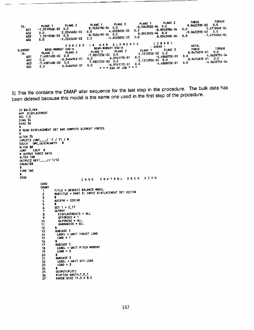
ID. PLANE 1 PLANE 2 PLANE 1 PLANE 2 PLANE 1 PLANE 2 FORCE TORQUE601 -1.551956E-03 0.0 8.763619E-0_ 0.0 -8.094392E-04 O.O 9.962239E-02 0.0602 O.O 2.224563E-03 0.0 4.652883E- 03 O.O -B.O9439BE- 04 0.0 1.471004E-04603 1.551956E-03 0.0 -8.7636192-04 0.0 8.094392E-04 0.0 -9.962Z39E-02 0.0
604 0.0 -2.224563E-03 0.0 -4.652883E-03 0.0 8.0943982- 04 0.0 -1.471004E-04
FORCES I N BAR ELEMENTS (CBAR)ELEMENT BEND-MOMENT END-A BEND-MOMENT END-B - SHEAR - AXIAL
ID. PLANE 1 PLANE 2 PLANE 1 PLANE 2 PLANE 1 PLANE 2 FORCE TORQUE601 7.4061482-02 0.0 -7.985723E-02 0.0 5.131290E-02 0.0 B.947487E-01 O.O602 0.0 -6.546494E-01 0.0 6.914117E-01 0.0 -4.486870E-01 0.0 4.063973E- 04603 -7.408148E-02 0.0 7.9857232-02 0.0 -5.131290E-02 O.O -8.9474872-01 O.O604 0.0 6.546494E-01 0.0 -6.914117E-01 0.0 4.48687'0E- 01 0,0 -4.063975E-04
t * * END OF JOB * * *
5) This file contains the DMAP alter sequence for the last step in the procedure. The bulk data has
been deleted because this model is the same one used in the first step of the procedure.
ID BAL3,FEMAPP DISPLACEHENT
SOL 1,0DIAG 14DIAG 36$$ READ DISPLACEMENT SET AND COMPUTE ELEMENT FORCES$ALTER 7'5
INPUTT2 ILIHC, oo,/ "1 / 11 / $EOUIV UMC,ULV/ALWAYS $ALTER 88JUMP LBL9 $$ OUTPUT FORCE DATAALTER 108
OUTPUTZ 0EF1,,,,1/-1/12ENDALTER$
TIME 160$
CEHD
CARDCOUNT
I2
3456789
1011
1213
141516171819
20212223242526Z7
CASE CONTROL DECK E C HO
TITLE = GENERIC BALANCE MODELSUBTITLE = PART 3: INPUT DISPLACEMENT SET VECTOR$
AXISYM = COSINE$
SET 1 = 2,17OUTPUT
DISPLACEMENTS = ALLGPFORCES = 1ELFORCES • ALLHARMONICS • ALL
$SUBCASE 1
LABEL = UNiT THRUST LOADLOAD = 1
$SUBCASE 2
LABEL = UNIT PITCH MOMENTLOAD = 2
$
SUBCASE 3LABEL = UNIT AFT LOADLOAD = 3
$
OUTPUT(PLOT)PLOTTER NASTPLT,D,1PAPER SIZE 11.0 X 8.5
157
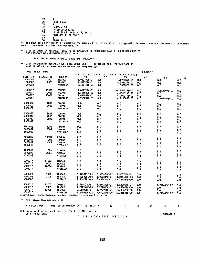
28 $
SET 1 ALL30 $
31 AXES X,Y,Z32 VIEW 90.,90.,0.33 FIND SCALE, ORIGIN 11, SET 134 PLOT SET 1, ORIGIN 1135 $36 BEGIN BULK
<< The bulk data for this file is exactly the same as file Listing #3 in this appendix, because these ere the same finite elementn_xJets. The bulk date has been deleted. >>
*** USER INFORMATION MESSAGE - GRID-POINT RESEQUENCING PROCESSOR BANDIT IS NOT USED DUE TOTHE PRESENCE OF AXISYIM4ETRIC SOLID DATA
**NO ERRORS FOUND - EXECUTE NASTRAN PROGRAM**
*** USER INFORMATION MESSAGE 4105, DATA BLOCK UNC RETRIEVED FROM FORTRAN TAPE 11NN4E OF DATA BLOCK WHEN PLACED ON FORTRAN TAPE WAS ULV
UNIT THRUST LOAD SUBCASE 1GR ] D PO I N T FORCE BALANCE
POINT-ID ELEMENT- iD S(XJRCE T1 T2 T3 R1 R21000002 1001 TRAPAX -1.962777E-01 0.0 4.697984E -01 0.0 0.0 0.01000002 2001 TRAPAX 1.987579E-01 0.0 5.30203ZE-01 0.0 0.0 0.01000002 tTOTALS* 2.480194E-03 0.0 1.000002E+O0 0.0 0.0 0.0
R3
1000017 11001 CONEAX 3.862712E+01 0.0 -4.880019E+01 0.0 2.665097E+00 0.01000017 9001 TRAPAX -1.411920E-02 0.0 -4.058314E-01 0.0 0.0 0.01000017 10001 TRAPAX 3.094939E+01 0.0 4.290217E+00 0.0 0.0 O.O
1000017 *TOTALS* 6.956239E*01 0.0 -4.491580E+01 0.0 2.665097E+00 0.0
2000002 1002 TRAPAX 0.0 0.0 0.0 0.0 0.0 0.02000002 2002 TRAPAX 0.0 0.0 0.0 0.0 0.0 0.02000002 *TOTALS* O.O 0.0 0.0 0.0 O.O 0.0
2000017 11002 CONEAX 0.0 0.0 0.0 0.0 0.0 0.02000017 9002 TRAPAX 0.0 0.0 0.0 0.0 0.0 0.02000017 10002 TRAPAX 0.0 0.0 0.0 0.0 0.0 0.0
2000017 *TOTALS* 0.0 0.0 0.0 0.0 0.0 0.0
3000002 1003 TRAPAX 0.0 0.0 0.0 0.0 0.0 0.03000002 2003 TRAPAX 0.0 0.0 0.0 O.O 0.0 0.03000002 *TOTALS* 0.0 0.0 O.O O.O 0.0 0.0
3000017 11003 CONEAX 0.0 0.0 0.0 0.0 0.0 0.0
3000017 9003 TRAPAX 0.0 0.0 0.0 0.0 0.0 0.0
3000017 10003 TRAPAX 0.0 0.0 0.0 0.0 0.0 0.03000017 *TOTALS* 0.0 0.0 0.0 0.0 0.0 0.0
4000002 1004 TRAPAX 0.0 0.0 0.0 0.0 0.0 0.0
4000002 2004 TRAPAX 0.0 0.0 0.0 0.0 0.0 0.0
4000002 *TOTALS* 0.0 0.0 0.0 0.0 0.0 0.0
4000017 110044 CONEAX 0.0 0.0 0.0 0.0 0.0 0.04000017 9004 TRAPAX 0.0 0.0 0.0 O.O 0.0 0.04000017 10004 TRAPAX 0.0 0.0 0.0 0.0 0.0 0.04000017 *TOTALS* 0.0 0.0 0.0 0.0 0.0 0.0
5000002 1005 TRAPAX -3.393911E-01 -6.053476E-02 -2.903760E-01 0.0 0.0 O.O
5000002 2005 TRAPAX -1.026829E+00 6.023814E-01 -1.034488E+00 0.0 0.0 0.05000002 *TOTALS* -1.366220E+00 5.418466E-01 -1.324864E+00 0.0 0.0 0.0
5000017 11005 CONEAX 2.364401E-01 -3.854312E-01 -2.812054E-01 0.0 3.798493E-02 0.0
5000017 9005 TRAPAX -1.272544E+00 -7.269861E-01 -1.453672E+00 0.0 0.0 0.05000017 10005 TRAPAX 9.631046E-01 -3.777996E-01 -1.490628E+00 0.0 0.0 0.05000017 *TOTALS* -7.2_60E-02 -1.490217E+00 -3.225505E+00 0.0 3.798493E-02 0.0
<< Grid point force balance has been Limited to subcase 1 only. >>
*** USER INFORMATION MESSAGE 4114
DATA BLOCK _FI WRITTEN ON FORTRAN UNIT 12, TRLR = 63 I 16 91 6 I
<< Displacement output is limited to the first 10 rings. >>UNIT THRUST LOAD
D I SPLACENENT VECTORSUBCASE 1
158
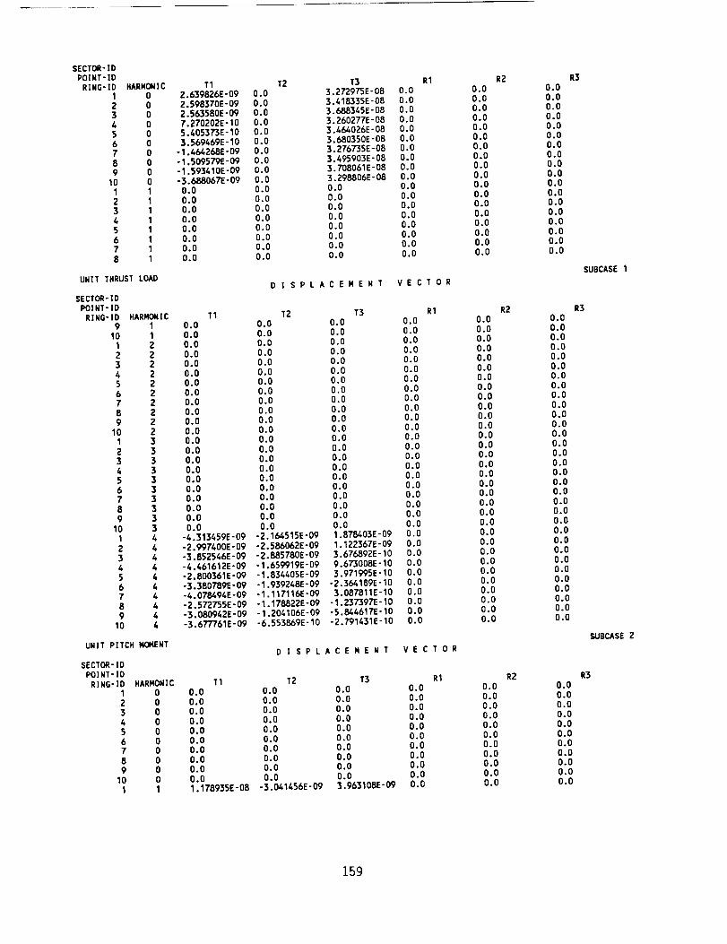
SECTOA-IDPOINT-ID
RING-ID HARMONIC1 0
2 03 04 05 0
6 07 0
8 09 0
10 01 12 13 14 15 16 17 18 1
UNIT THRUST LOAD
T12.639826E-09 O. 0E. 598370E-09 0.02.5635BOE-09 O. 07.270202E- 10 0.05.405373E- 10 0.03. 569469E- 10 O. 0
-1.46_268E- 09 0.0-1 , 509579E-09 0.0-1,593410E-09 0.0-3.688067E- 09 0.0
0.0 0.00.0 0.00.0 0.00.0 0.00.0 0.00.0 0.00.0 0.0
0.0 0.0
SECTOR- %DPOl NT- ID
RING-ID HARNON! C T19 1 0.0
10 1 0.01 Z 0.02 2 0.03 2 0.04 2 0.05 2 0.06 2 0.0
7 2 0.08 2 0.09 2 0.0
10 2 0.01 3 0.0
2 3 0.0
3 3 0.04 3 0.05 3 0.06 3 O.O7 3 0.08 3 0.09 3 0.0
10 3 0.01 4
2 43 44 45 46 4? 48 49 4
10 4
UNIT PITCH MOMENT
T2 T3 R13.27297'5 E - 08 O. 03.418335E-08 0.03.688345E- 08 0.03. 260277E- 08 O. 03.464026E-08 0.03.6_0350E-08 0.03.276735E-08 0.03.495903E-08 O.O3. ?'08061E- 08 0.03. 298806E - 08 0.00.0 0.00.0 0.00.0 0.00.0 0.00.0 0.0
0.0 0.0
0.0 0.0
0.0 O.O
DISPLACEMENT VECTOR
0.00.00.00.00.00.00.00.00.0
0.00.00.00.00.00.00.00.00.00.0
0.00.0
0.0
T2 T3 R10.0 0.00.0 0.00.0 0.00.0 0.00.0 0.00.0 0.00.0 0.0
0.0 0.00.0 0.0
0.0 0.0
0.0 0.0
0.0 0.0
0.0 0.0
0.0 0.00.0 O.O
0.0 0.00.0 0.00.0 0.00.0 0.00.0 0.00.0 0.00.0 0.0
-4.313459E-09 -2.164515E-09 1.878403E-09 0.0
-2.997400E-09 -2.586062E-09 I.122367E-09 0.0
-3.852546E-09 -2.885780E- 09 3.676892E- I0 0.0
-4. 461612E -09 -I.659919E -09 9.6_008E -I0 O.0
-2.800361E-09 -I.834405E-09 3.971_5E-I0 0,0
-3.380789E-09 -1.939248E-09 -2.364189E-10 0.0-4. 078_94E-09 -1. 117116E-09 3.087811E- 10 0.0-2.572755E-09 -1.178822E-09 -1.237397E-10 0.0-3.080942E-09 -1.204106E-09 -5.844617E-10 0.0-3.677761E-09 -6.553869E-10 -2.791431E-10 0.0
SECTOR- IDPOINT-IDRING- ID HARMONIC
I 0 0.0
2 0 0.0
3 0 0.04 0 0.05 0 0.06 0 0.0
7 0 0.08 0 0.09 0 0.0
10 0 0.01 1
DISPLACEMENT VECTOR
TI T2 T3 RI0.0 0.0 0.00.0 0.0 0.00.0 0.0 0.00.0 0.0 0.00.0 0.0 0.00.0 0.0 0.0
0.0 0.0 0.0
0.0 0.0 0.0
0.0 0.0 0.0
0.0 0.0 0,01.178935E-08 -3.041456E-09 3.963108E-09 0.0
0.00.00.00.00.00.00.00.00.00.00.00.00.00.00.00.00.0
0.0
0.00.00.00.00.00.00.0
0.00.00.00.00.00.00.00.0
0.00.00.00.00.00.00.00.0
0.00.00.00.00.00.00.00.00.0
0.00.00.00.00.00.00.00.00.0
0.00.0
R2
R2
R2
0.00.00.00.00.00.00.00.00.00.00.00.00.00.00.00.0
0.00.0
0.00.00.00.00.0
0.00.0
0.00.00.00.00.00.00.00.0
0.00.00.00.00.00.00.00.00.0
0.00.00.00.00.00.00.00.0
R3
R3
SUBCASE I
R30.00.00.0
0.00.0
0.00.00.00.00.00.0
,_dJBCASE 2
159
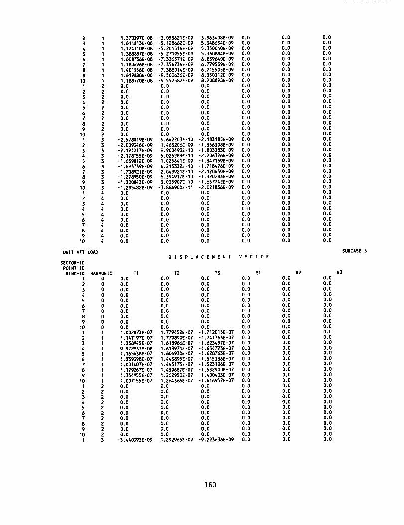
2 13 14 15 16 17 18 19 1
10 11 22 Z3 Z4 25 Z
6 27 28 29 2
10 21 32 33 34 35 36 37 3
8 39 3
10 31 6,Z 43 44 45 46 47 48 49 4
10 4
UNIT AFT LOAD
SECTOR- IDPOINT- ID
RING- ]D HARMONIC1 0 0.0
2 0 0.03 0 0.0
4 0 0.05 0 0.06 0 0.07 0 0.08 0 0.09 0 0.0
10 0 0.01 12 13 14 15 1
6 17 1
8 19 1
10 11 2 0.02 2 0.03 2 0.04 2 0.05 2 0.06 2 0.0
7 2 0.0
8 2 0.09 2 0.0
10 2 0.01 3
1.370397E-08 -3.053621E-09 3.963408E-09 0.01.611813E-08 -5.128662E-09 5.348634E-09 0.01.174310E-08 -5.201514E-09 5.350040E-09 0.01.388887E-08 -5.271955E-09 5.360884E-09 0.01.608736E-08 -7.336571E-09 6.839640E-09 0.0
1.180696E-08 -7.354734E-09 6.779539E-09 0.01.401556E-08 -7.388014E-09 6.715505E-09 0.01.619888E-08 -9.560636E-09 8.350312E-09 0.01.188170E-08 -9.552582E-09 8.208898E-09 0.00.0 0.0 0.0 0.0
0.0 0.0 0.0 0.0
0.0 0.0 0.0 0,0
0.0 0.0 0.0 0.0
0.0 0.0 0.0 0.0
0.0 0.0 0.0 0.0
0.0 0.0 0.0 0.0
0.0 0.0 0.0 0.0
0.0 0.0 0.0 0.0
0.0 0.0 0.0 0.0
-2.578819E-09 9.642203E-10 -2.183185E-09 0.0
-2.009546E-09 1.463206E-09 -1.356308E-09 0.0-2.121217E-09 9.900493E-10 -1.803383E-09 0.0-2.178755E-09 5.026283E-10 -2.206326E-09 0.0-1.639812E-09 1.025641E-09 -1.347159E-09 0.0-1.693759E-09 6.213332E-10 -1.718476E-09 0.0-1.708921E-09 2.049921E-10 -2.120450E-09 0.0-1.278950E-09 6.394917E-10 -1.320283E-09 0.0-1.300843E-09 3.035907E-10 -1.657742E-09 0.0-1.295482E-09 -3.866900E-11 -2.021836E-09 0.00.0 0.0 0.0 0.0
0.0 0.0 0.0 0.0
0.0 0.0 0.0 0.0
0.0 0.0 0.0 0.0
0.0 0.0 0.0 0.00.0 0.0 0.0 0.00.0 0.0 0,0 0.00.0 0.0 0.0 0.00.0 0.0 0.0 0.00.0 0.0 0.0 0.0
DISPLACEMENT VECTOR
T1 T2 T3 R10.0 0.0 0.00.0 0.0 0.00.0 0.0 0.0
0.0 0.0 0.00.0 0.0 0.00.0 0.0 0.0
0.0 0.0 0.0
0.0 0.0 0.0
0.0 0.0 0.0
0.0 0.0 0.0
1.002073E-07 1.779452E-07 -1.712015E-07 0.0
1.147197E-07 1.779890E-07 -1.741763E-07 0.0
1.338945E-07 1.618966E-07 -1.623457E-07 0.0
9.972933E-08 1.613971E-07 -1.634T23E-07 0.01.165638E-07 1.606930E-07 -1.628763E-07 0.01.339398E-07 1.443895E-07 -1.515336E-07 0.01.001607E-07 1.463175E-07 -1.523106E-07 0.01.179267E-07 1.439687E-07 -1.532900E-07 0.01.356955E-07 1.262950E-07 -1.400403E-07 0.0
1.007155E-07 1.264366E-07 -1.416957E-07 0.00.0 0.0 0.0
0.0 0.0 0.00.0 0.0 0.0
0.0 0.0 0.0
0.0 0.0 0.0
0.0 0.0 0.00.0 0.0 0.0
0.0 0.0 0.00.0 0.0 0.00.0 0.0 0.0
-5.660393E-09 1.292965E-09 -9.223636E-09 0.0
0.00.0
0.00.00.00.00.00.00.00.00.00.00.00.00.00.00.00.0
0.00.0
0.00.00.00.00.00.00.00.00.00.00.00.0
0.00.0
0.00.00.00.00.0
R20.00.0
0.00.00.00.00.00.00.00.00.00.00.0
0.00.00.00.00.0
0.00.00.00.00.00.00.00.00.00.00.00.00.0
0.00.0
0.0
0.0
0.0
0.0
0.00.0
0.0
0.0
0.0
0.0
0.0
0.0
0.0
0.0
0.0
0.0
0.0
0.0
0.0
0.0
0.0
0.0
0.0
0.0
0.0
0.0
0.0
0.0
0.0
0.0
0.0
0.0
0.0
0.0
0.0
0.0
0.0
0.0
0.0
0.0
0.0
0.0
0.0
0.0
0.0
0.0
0.0
0.0
0.0
0.0
0.0
0.0
0.0
0.0
0.0
0.0
0.0
0.0
0.0
0.0
0.0
0.0
0.0
0.0
0.00.0
0.0
0.0
SUBCASE 3
R3
160
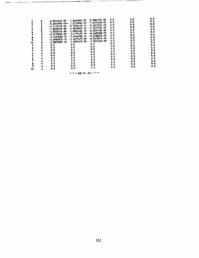
23456789
10123456789
10
3333333334444444444
-3.301694E-09 1.366266E-09 -5.586073E-09 0.0-3.683499E-09,,_, 1.212996E-09 -7.655163E-09 0.0-4.111131E-09 -5.739011E-10 -9.287293E-09 0.0- 1.839876E-09 /,. 98189P,E- 10 -5.637970E-09 0.0-1.950501E-09 -1.892448E-10 -6.9S9178E-09 0.0-2.077800E-09 -7.417547E-10 -8.568358E-09 0.0-4.745768E-10 -7.674623E-10 -5.218832E-09 0.0-4.650081E-10 -1.067167E-09 -6.521891E-09 0.0-5.085589E-10 -1.359747E-09 -7.921546E-09 0.0
0.0 0.0 0.0 0.00.0 0.0 0.0 0.00.0 0.0 0.0 0.00.0 0.0 0.0 0.00.0 0.0 0.0 0.00.0 0.0 0.0 0.00.0 0.0 0.0 0.00.0 0.0 0.0 0.00.0 0.0 0.0 0.00.0 0.0 0.0 0.0
* * * END OF JOB " * *
0.00.00.00.00.00.00.00.00.00.00.00.00.00.00.00.00.00.00.0
0.00.00.00,00.00.00.00.00.00.00.00.00.00.00.00.00.00,00.0
161
N91-20517
Finite Element Solution of Transient
Fluid-Structure Interaction Problems
Gordon C. Everstinc, Raymond S. Cheng, and Stephen A. Hambric
Computational Mechanics Division (128)
David Taylor Research Center
Bethesda, Maryland 20084
ABSTRACT
A finite element approach using NASTRAN is developed for solving time-dependent fluid-
structure interaction problems, with emphasis on the transient scattering of acoustic waves from
submerged elastic structures. Finite elements are used for modeling both structure and fluid domains
to facilitate the graphical display of the wave motion through both media. For the fluid, the use of
velocity potential as the fundamental unknown results in a symmetric matrix equation. The approach
is illustrated for the problem of transient scattering from a submerged elastic spherical shell subjected
to an incident tone burst. The use of an analogy between the equations of elasticity and the wave
equation of acoustics, a necessary ingredient to the procedure, is summarized.
INTRODUCTION
Computational structural acoustics is concerned with the prediction of the acoustic pressure
field radiated or scattered by submerged structures subjected to either mechanical or external (fluid)
excitation. When the excitation is time-harmonic, the most common numerical approach for solving
the interaction problem is to couple a finite element model of the structure with a boundary element
model of the surrounding fluid (Ref. 1-8). Other fluid modeling approaches have inchlded finite
element (Ref. 9-20), combined finite element/analytical (Ref. 21-23), and T-matrix (Ref. 24-26).
For time domain (transient) analysis, there are several computational approaches which can beused:
• the transformation of frequency domain results to the time domain using the Fourier transform
• the use of a fluid loading approximation such as the doubly asymptotic approximation (DAA)(Ref. 27)
• the time domain boundary element approach, which models the fluid with the retarded potentialintegral equation (Ref. 28-31)
• the fluid finite element approach, which models the exterior fluid domain with finite elements
truncated at a finite distance from the structure and terminated with an approximate radiation
boundary condition to absorb outgoing waves (Ref. 9-20)
To our knowledge, the retarded potential integral equation has been used only for special geometries
(e.g., axisymmetry) because of the method's relatively high computational cost. The DAA approach,
which has been used successfully in underwater shock analysis (Ref. 32-34), may not be adequate fortransient acoustics, where the interest is in the response in the fluid as well as in the structure. The
principal computational trade-off between the fluid finite element approach and the other three
approaches is that the finite element approach yields large, banded matrices, whereas the other three
162
approaches (which depend on boundary clement calculations) yield smaller, densely-populatedmatrices. This trade-off often favors the finite element approach for long, slender structures like
ships which are "naturally banded." In addition, of the four approaches listed, only the fluid finite
element approach has directly available an explicit fluid mesh which can be used for graphical displayof the wave motion through the fluid. Since a significant part of our interest involves the display of
wave propagation through both structure and fuid, we therefore formulate the transient acoustics
problem using the fluid finite clement approach. The principal drawbacks to a fluid finite element
approach are the need for an approximate radiation boundary condition at the outer fluid boundary,
the requirements on mesh size and extent (sometimes leading to frequency-dependent fluid meshes
(Ref. 17)), and the difficulty of generating the fluid mesh.
Dynamics problems involving the interaction between an elastic structure and an acoustic fluidhave been forlnulated for finite element solution using pressure (Ref. 9,10), fluid particle
displacenlent (Ref. 11-13,15,17), displacement potential (Ref. 16), and velocity potential (Ref. 18,19)as the fundamental unknown in the fluid region. In three dimensions, the pressure and displacement
formulations result in, respectively, one and three degrees of freedom per finite element mesh point.
Thus the pressure approach has the advantage of fewer unknowns and a smaller overall matrix profile
or bandwidth if the grid points are properly sequenced. On the other hand, the displacement
approach results in symmetric coefficient matrices (in contrast to the pressure formulation, for which
the matrices are nonsymmetric) and a lhfid-structure interface condition which is easier to implement
with general purpose finite element computer programs. However, the displacement approach also
suffers from the presence of spurious resonances (Ref. 15), a situation which can be bothersome in
time-harmonic problems, either forced or unforced. The principal disadvantage of the pressure
fornmlation, nonsymmetric coefficient matrices, can be removed merely by rcformnlating the pressure
solution approach so that a velocity potential rather than pressure is used as the fundamental
unknown in the fluid region (Ref. 18). For some situations, particularly time-harmonic problems
involving damped systems and time-dependent problems, significant computational advantages result.
The principal goal of this paper is to develop in detail the symmetric velocity potential
formulation for application to the specific problem of transient acoustic scattering from submerged
elastic structures. Previously (Ref. 18), the symmetric potential formulation was described only in
general terms for a wide class of fluid-structure interaction problems with no details concerning
specific types of applications such as vibrations, shock response, or acoustic scattering.
From an engineering point of view, it is convenient to be able to make use of existing general
purpose finite element codes such as NASTRAN, because of their wide availablity, versatility,
reliability, consultative support, and abundance of pre- and postprocessors. Thus the next section
summarizes an analogy between the equations of elasticity and the wave equation of acoustics. Such
an analogy allows the coupled structural acoustic problem to be solved with standard finite element
codes.
STRUCTURAL-ACOUSTIC ANALOGY
Since we wish to solve the coupled structural acoustic problem using standard finite element
codes, we summarize here the application of such codes to the wave equation of acoustics (Ref.
35,36),
VZp = p/c 2,
where V: is the Laplacian operator, p is the dynamic fluid pressure, c is the wave speed, and dots
denote partial differentiation with respect to time.
On the other hand, the x-component of the Navier equations of elasticity, which are the
equations solved by structural analysis computer programs, is
(1)
163
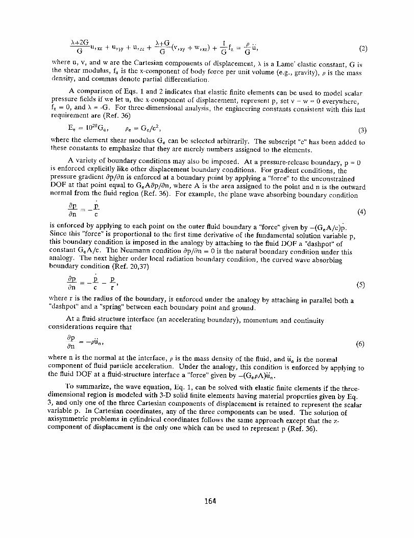
X+2G X+G "r 1 --g-PiJ (2) u,xx + U,yr+ u,z + ,xy+ w,xz) + -fx = o '
where u, v, and w are the Cartesian components of displacement, X is a Lame" elastic constant, G is
the shear modulus, fx is the x-component of body force per unit volume (e.g., gravity), p is the mass
density, and commas denote partial differentiation.
A comparison of Eqs. 1 and 2 indicates that elastic finite elements can be used to model scalar
pressure fields if we let u, the x-component of displacement, represent p, set v = w = 0 everywhere,
fx = 0, and X = -G. For three-dimensional analysis, the engineering constants consistent with this last
reqnirement are (Ref. 36)
Ee = 10Z°G_, pe = G_/c 2, (3)
where the element shear modulus Ge can be selected arbitrarily. The subscript "e" has been added to
these constants to emphasize that they are merely numbers assigned to the elements.
A variety of boundary conditions may also be imposed. At a pressure-release boundary, p = 0
is enforced explicitly like other displacement boundary conditions. For gradient conditions, the
pressure gradient 0p/0n is enforced at a boundary point by applying a "force" to the unconstrained
DOF at that point equal to G_A0p/0n, where A is the area assigned to the point and n is the outward
normal from the fluid region (Ref. 36). For example, the plane wave absorbing boundary condition
0_p_ = __p_ (4)On c
is enforced by applying to each point on the outer fluid boundary a "force" given by -(G_A/c)p.
Since this "force" is proportional to the first time derivative of the fundamental solution variable p,
this boundary condition is imposed in the analogy by attaching to the fluid DOF a "dashpot" of
constant GeA/c. The Neumann condition 0p/0n = 0 is the natural boundary condition under this
analogy. The next higher order local radiation boundary condition, the curved wave absorbing
boundary condition (Ref. 20,37)
=--P- - -P--, (5)On c r
where r is the radius of the boundary, is enforced under the analogy by attaching in parallel both a
"dashpot" and a "spring" between each boundary point and ground.
At a fluid-structure interface (an accelerating boundary), momentum and continuity
considerations require that
0__p_= -piJ,, (6)On
where n is the normal at the interface, p is the mass density of the fluid, and i/n is the normal
component of fluid particle acceleration. Under the analogy, this condition is enforced by applying to
the fluid DOF at a fluid-structure interface a "force" given by -(G_pA)i/,.
To summarize, the wave equation, Eq. 1, can be solved with elastic finite elements if the three-
dimensional region is modeled with 3-D solid finite elements having material properties given by Eq.
3, and only one of the three Cartesian components of displacement is retained to represent the scalar
variable p. In Cartesian coordinates, any of the three components can be used. The solution of
axisymmetric problems in cylindrical coordinates follows the same approach except that the z-component of displacement is the only one which can be used to represent p (Ref. 36).
164
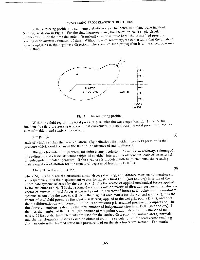
SCATTERING FROM ELASTIC STRUCTURES
In the scattering problem, a submerged elastic body is subjected to a plane wave incidentloading, as shown in Fig. 1. For the time-harmonic case, the excitation has a single circularfrequency 0a. For the time-dependent (transient) case of interest here, the prescribed pressure
loading is an arbitrary function of time. Without loss of generality, we can assume that the incidentwave propagates in the negative z direction. The speed of such propagation is c, the speed of soundin the fluid.
o
ER
PLANE
WAVE
Fig. 1. The scattering problem.
Within the fluid region, the total pressure p satisfies the wave equation, Eq. 1. Since theincident free-field pressure Pi is known, it is convenient to decompose the total pressure p into thesum of incident and scattered pressures
p = pi + ps, (7)
each of which satisfies the wave equation. (By definition, the incident free-field pressure is thatpressure which would occur in the fluid in the absence of any scatterer.)
We now formulate the problem for finite element solution. Consider an arbitrary, submerged,three-dimensional elastic structure subjected to either internal time-dependent loads or an external
time-dependent incident pressure. If the structure is modeled with finite elements, the resultingmatrix equation of motion for the structural degrees of freedom (DOF) is
Mii + Bti + Ku = F - GAp, (8)
where M, B, and K are the structural mass, viscous damping, and stiffness matrices (dimension s xs), respectively, u is the displacement vector for all structural DOF (wet and dry) in terms of the
coordinate systems selected by the user (s x r), F is the vector of applied mechanical forces appliedto the structure (s x r), G is the rectangular transformation matrix of direction cosines to transform avector of outward normal forces at the wet points to a vector of forces at all points in the coordinatesystems selected by the user (s x f), A is the diagonal area matrix for the wet surface (f x f), p is thevector of total fluid pressures (incident + scattered) applied at the wet grid points (f x r), and dotsdenote differentiation with respect to time. The pressure p is assumed positive in compression. Inthe above dimensions, s denotes the total number of independent structural DOF (wet and dry), fdenotes the number of fluid DOF (the number of wet points), and r denotes the number of loadcases. If first order finite elements are used for the surface discretization, surface areas, normals,and the transformation matrix G can be obtained from the calculation of the load vector resultingfrom an outwardly directed static unit pressure load on the structure's wet surface. The matrix
165
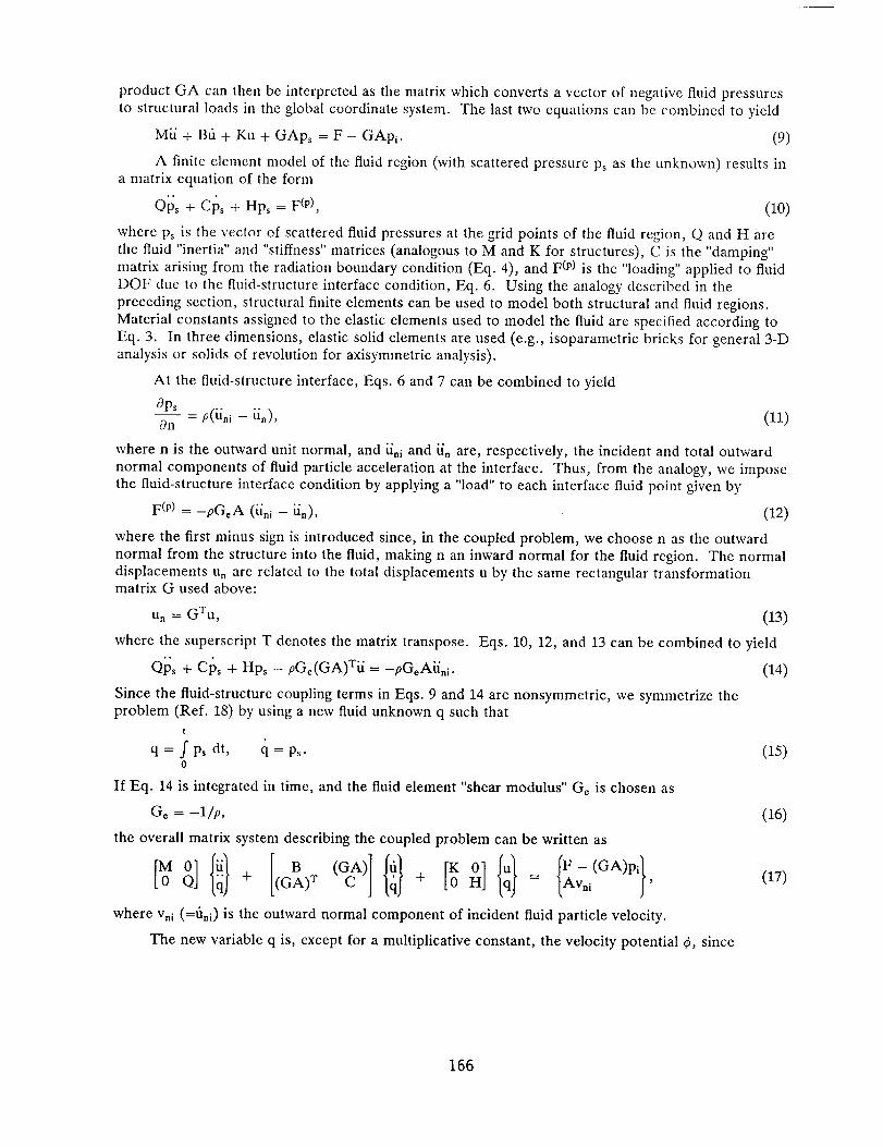
product GA can then be interpreted as the matrix which converts a vector of negative fluid pressures
to structural loads in the global coordinate system. The last two equations can be combined to yield
M{i + Bfl + Ku + GAps = F- GApi. (9)
A finite element model of the fluid region (with scattered pressure Ps as the unknown) results ina matrix equation of the form
OPs + Cps + Hp, = F (p), (10)
where Ps is the vector of scattered fluid pressures at the grid points of the fluid region, Q and H are
the fluid "inertia" and "stiffness" matrices (analogous to M and K for structures), C is the "damping"matrix arising from the radiation boundary condition (Eq. 4), and F (p) is the "loading" applied to fluid
DOF due to the fluid-structure interface condition, Eq. 6. Using the analogy described in the
preceding section, structural finite elements can be used to model both structural and fluid regions.
Material constants assigned to the elastic elements used to model the fluid are specified according to
Eq. 3. In three dimensions, elastic solid elements are used (e.g., isoparametric bricks for general 3-Danalysis or solids of revolution for axisymmetric analysis).
At the fluid-structure interface, Eqs. 6 and 7 can be combined to yield
OPs- p(iini - iin), (11)011
where n is the outward unit normal, and iini and iin are, respectively, the incident and total outward
normal components of fluid particle acceleration at the interface. Thus, from the analogy, we imposethe fluid-structure interface condition by applying a "load" to each interface fluid point given by
F (p) = -pGeA (iini - iin), (12)
where the first minus sign is introduced since, in the coupled problem, we choose n as the outward
normal from the structure into the fluid, making n an inward normal for the fluid region. The normaldisplacements Un are related to the total displacements u by the same rectangular transformationmatrix G used above:
un = G xu, (13)
where the superscript T denotes the matrix transpose. Eqs. 10, 12, and 13 can be combined to yield
Ops + Cps + Hps - pGe(GA)Xii = -pGeAiini. (14)
Since the fluid-structure coupling terms in Eqs. 9 and 14 are nonsymmetric, we symmetrize theproblem (Ref. 18) by using a new fluid unknown q such that
t
q = f Ps dt, q = Ps- (15)0
If Eq. 14 is integrated in time, and the fluid element "shear modulus" G_ is chosen as
Ge = -I/p, (16)
the overall matrix system describing the coupled problem can be written as
[0where Vni
The
_] {_} + [(GB) T (GcA)] {_} + [_0 H0] {q} = J'F-(GA)pil[Av,, j,(=fi_i) is the outward normal component of incident fluid particle velocity.
new variable q is, except for a multiplicative constant, the velocity potential _, since
(17)
166
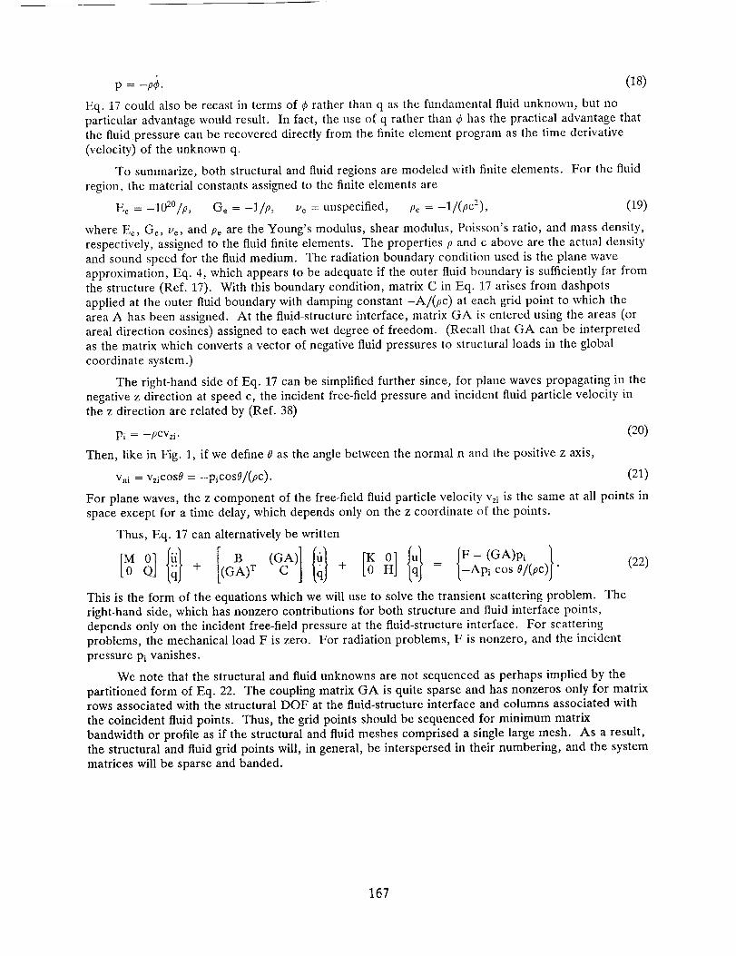
p = _/. (is)
Eq. 17 could also be recast in terms of _ rather than q as the fundamental fluid unknown, but no
particular advantage would result. In fact, the use of q rather than _bhas the practical advantage that
the fluid pressure can be recovered directly from the finite element program as the time derivative
(velocity) of the unknown q.
To summarize, both structural and fluid regions are modeled with finite elements. For the fluid
region, the material constants assigned to the finite elements are
Ee = -102°/p, Ge = -l/p, ue = unspecified, Pe = -1/(pc2), (19)
where Ee, Ge, re, and Pe are the Young's modulus, shear modulus, Poisson's ratio, and mass density,
respectively, assigned to the fluid finite elements. The properties p and c above are the actual density
and sound speed for the fluid medium. The radiation boundary condition used is the plane wave
approximation, Eq. 4, which appears to be adequate if the outer fluid boundary is sufficiently far from
the structure (Ref. 17). With this boundary condition, matrix C in Eq. 17 arises from dashpots
applied at the outer fluid boundary with damping constant -A/(pc) at each grid point to which the
area A has been assigned. At the fluid-structure interface, matrix GA is entered using the areas (or
areal direction cosines) assigned to each wet degree of freedom. (Recall that GA can be interpretedas the matrix which converts a vector of negative fluid pressures to structural loads in the global
coordinate system.)
The right-hand side of Eq. 17 can be simplified further since, for plane waves propagating in the
negative z direction at speed c, the incident free-field pressure and incident fluid particle velocity in
the z direction are related by (Ref. 38)
Pi = --pCVzi. (20)
Then, like in Fig. 1, if we define 0 as the angle between the normal n and the positive z axis,
Vni = VziCOS0 = -picosO/(pc). (21)
For plane waves, the z component of the free-field fluid particle velocity vzi is the same at all points in
space except for a time delay, which depends only on the z coordinate of the points.
Thus, Eq. 17 can alternatively be written
[M (_] {_} + [(GB).r (GcA) ] {_} + [K O] {q} = fF-(GA)pil-Api cos o/(pc) (22)
This is the form of the equations which we will use to solve the transient scattering problem. The
right-hand side, which has nonzero contributions for both structure and fluid interface points,
depends only on the incident free-field pressure at the fluid-structure interface. For scattering
problems, the mechanical load F is zero. For radiation problems, F is nonzero, and the incident
pressure Pi vanishes.
We note that the structural and fluid unknowns are not sequenced as perhaps implied by the
partitioned form of Eq. 22. The coupling matrix GA is quite sparse and has nonzeros only for matrixrows associated with the structural DOF at the fluid-structure interface and columns associated with
the coincident fluid points. Thus, the grid points should be sequenced for minimum matrix
bandwidth or profile as if the structural and fluid meshes comprised a single large mesh. As a result,
the structural and fluid grid points will, in general, be interspersed in their numbering, and the system
matrices will be sparse and banded.
167
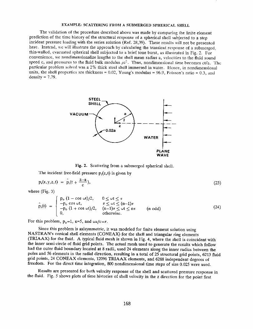
EXAMPLE: SCATTERING FROM A SUBMERGED SPHERICAL SHELL
The validation of the procedure described above was made by comparing the finite elementprediction of the time history of the structural response of a spherical shell subjected to a stepincident pressure loading with the series solution (Ref. 28,39). These results will not be presentedhere. Instead, we will illustrate the approach by calculating the transient response of a submerged,thin-walled, evacuated spherical shell subjected to a brief tone burst, as illustrated in Fig. 2. Forconvenience, we nondimensionalize lengths to the shell mean radius a, velocities to the fluid soundspeed c, and pressures to the fluid bulk modulus pc 2. Thus, nondimensional time becomes ct/a. Theparticular problem solved was a 2% thick steel shell immersed in water. Hence, in nondimensional
units, the shell properties are thickness = 0.02, Young's modulus = 96.9, Poisson's ratio = 0.3, anddensity = 7.79.
STEEL
SHEL_
VACUUM 0__z _WATER
PLANEWAVE
Fig. 2.
The incident free-field pressure pi(z,t) is given by
pi(x,y,z,t) = pi(t + z-a),c
where (Fig. 3)
Scattering from a submerged spherical shell.
(23)
Po (1 - cos _t)/2, 0_< _t < 7r
pi(t) = -Po cos 0Jt, _r_< wt _< (n-1)Tr-Po (1 + cos wt)/2, (n-1)rr < _t < nTr (n odd)0, otherwise.
For this problem, po=l, n=5, and wa/c=rr.
Since this problem is axisymmetric, it was modeled for finite element solution usingNASTRAN's conical shell elements (CONEAX) for the shell and triangular ring elements(TRIAAX) for the fluid. A typical fluid mesh is shown in Fig. 4, where the shell is coincident with
the inner semi-circle of fluid grid points. The actual mesh used to generate the results which followhad the outer fluid boundary located at 8 radii, used 24 elements along the inner radius between thepoles and 56 elements in the radial direction, resulting in a total of 25 structural grid points, 6213 fluidgrid points, 24 CONEAX elements, 12096 TRIAAX elements, and 6288 independent degrees offreedom. For the direct time integration, 800 nondimensional time steps of size 0.025 were used.
Results are presented for both velocity response of the shell and scattered pressure response inthe fluid. Fig. 5 shows plots of time histories of shell velocity in the z direction for the point first
(24)
168
1.5 i i i i
fflo_
(3_
-6t-O
if)r-
E
"13
It-O
7
1.0
0.5
0.0
-0.5
-1.0
-1.5
\l i | I
0.0 2.0 4-.0 6.0 8.0 10,0Non-dimensionel Time
Fig. 3. The incident pressure pi(t) (Eq. 24).
_,,'-r,2.fp%%'_, ,-X24_-/_' a _,,, -,
[_]"I r_Lr.}/ r_l_ i/kitk}_i_ifl i i
Fig. 4. Typical finite element mesh.
impacted by the pressure wave (O=0) and the back side pole (0=180 degrees). We observe from the
figure a significant oscillation in the back side of the shell. Back-scattered pressure time histories are
displayed in Fig. 6 at 3 and 5 radii from the origin. As expected, the scattered pressure at fluid
points is zero until the wave has had time to travel (at unit nondimensional speed) from the spherical
shell. Since the two points displayed are located 2 and 4 radii from the shell, the nondimensional
time delays for the scattered pressure wave to arrive are 2 and 4, respectively.
DISCUSSION
A practical procedure has been presented, using standard capabilities in NASTRAN, for
computing the solution of general time-dependent structural acoustics problems. Although illustrated
for the simple geometry of spherical shell scattering, there is no restriction in the approach to
particular geometries, so that any structure which can be modeled with NASTRAN can be handled.
169
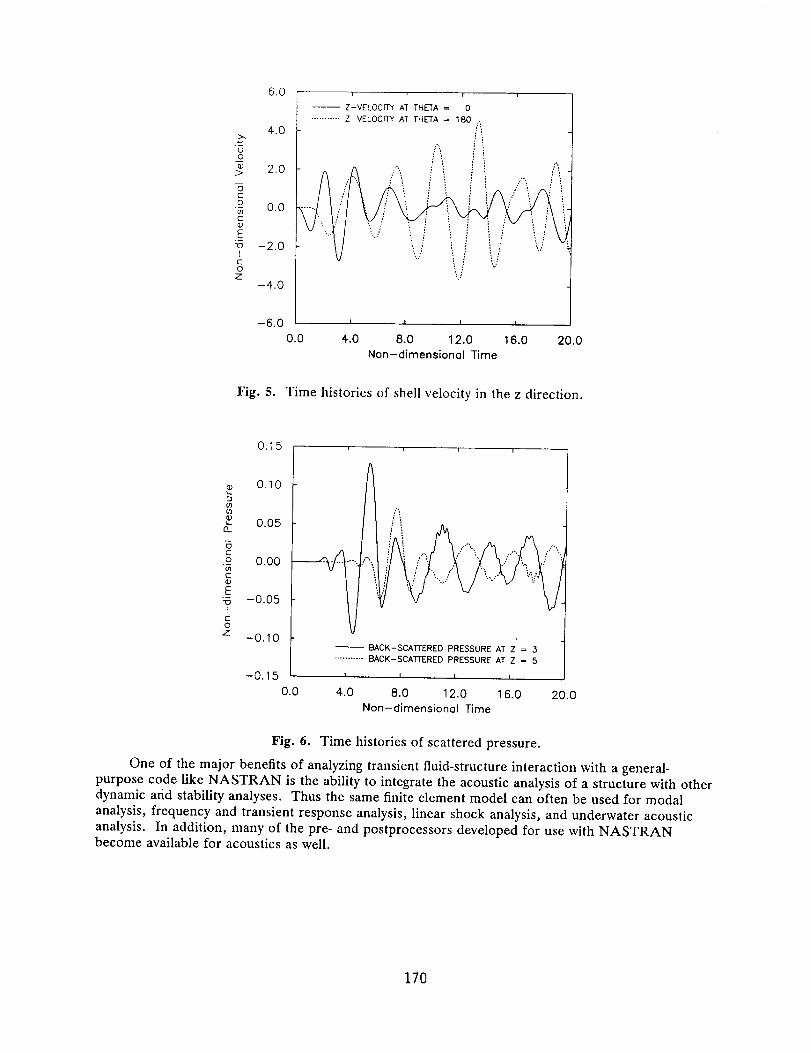
t.)O
_>
5c-O
c
E7O
CO
Z
6.0
4.0
2.0
0.0
-2.0
-4.0
i
-- Z-VELOCITY AT THETA = 0
........... Z-VELOCI'17' AT THETA = 180
:i f!
-6.0 I I I I
0.0 4.0 8.0 12.0 16.0 20.0Non-dimensional Time
Fig. 5. Time histories of shell velocity in the z direction.
co_o
13_
-5CO
ca)
E
t-O
Z
0,15
0.10
0.05
0.00
-0.05
-0.10
-0.15
-- BACK-SCA-PfERED PRESSURE AT Z = 3
...........BACK-SCAI-FERED PRESSURE AT Z = 5
I I I I
0.0 4.0 8.0 12.0 16.0
Non-dimensional Time20,0
Fig. 6. Time histories of scattered pressure.
One of the major benefits of analyzing transient fluid-structure interaction with a general-
purpose code like NASTRAN is the ability to integrate the acoustic analysis of a structure with other
dynamic and stability analyses. Thus the same finite element model can often be used for modal
analysis, frequency and transient response analysis, linear shock analysis, and underwater acoustic
analysis. In addition, many of the pre- and postprocessors developed for use with NASTRANbecome available for acoustics as well.
170
REFERENCES
1. L.H. Chen and D.G. Schweikert, "Sound Radiation from an Arbitrary Body," J. Aeoust. Soc.
Amer., Vol. 35, No. 10, pp. 1626-1632 (1963).
2. D.T. Wilton, "Acoustic Radiation and Scattering from Elastic Structures," Int. J. Num. Meth.in Engrg., Vol. 13, pp. 123-138 (1978).
3. J.S. Patel, "Radiation and Scattering from an Arbitrary Elastic Structure Using Consistent FluidStructure Formulation," Comput. Struct., Vol. 9, pp. 287-291 (1978).
4. I.C. Mathews, "Numerical Techniques for Three-Dimensional Steady-State Fluid-StructureInteraction," J. Acoust. Soc. Amer., Vol. 79, pp. 1317-1325 (1986).
5. G.C. Everstine, F.M. Henderson, E.A. Schroeder, and R.R. Lipman, "A General Low
Frequency Acoustic Radiation Capability for NASTRAN," Fourteenth NASTRAN Users'Colloquium, NASA CP-2419, National Aeronautics and Space Administration, Washington,
DC, pp. 293-310 (1986).
6. G.C. Everstine, F.M. Henderson, and L.S. Schuetz, "Coupled NASTRAN/Boundary ElementFormulation for Acoustic Scattering," Fifteenth NASTRAN Users' Colloquium, NASA CP-2481, National Aeronautics and Space Administration, Washington, DC, pp. 250-265 (1987).
7. A.F. Seybert, T.W. Wu, and X.F. Wu, "Radiation and Scattering of Acoustic Waves fromElastic Solids and Shells Using the Boundary Element Method," J. Acoust. Soc. Amer., Vol.84, pp. 1906-1912 (1988).
8. G.C. Everstine and F.M. Henderson, "Coupled Finite Element/Boundary Element Approachfor Fluid-Structure Interaction," J. Acoust. Soe. Amer., Vol. 87, No. 5, pp. 1938-1947 (1990).
9. O.C. Zienkiewicz and R.E. Newton, "Coupled Vibrations of a Structure Submerged in aCompressible Fluid," Proc. Internat. Symp. on Finite Element Techniques, Stuttgart, pp.359-379 (1969).
10. A. Craggs, "The Transient Response of a Coupled Plate-Acoustic System Using Plate andAcoustic Finite Elements," J. Sound and Vibration, Vol. 15, No. 4, pp. 509-528 (1971).
11. A.J. Kalinowski, "Fluid Structure Interaction," Shock and Vibration Computer Programs:Reviews and Summaries, SVM-10, ed. by W. Pilkey and B. Pilkey, The Shock and VibrationInformation Center, Naval Research Laboratory, Washington, DC, pp. 405-452 (1975).
12. L. Kiefling and G.C. Feng, "Fluid-Structure Finite Element Vibrational Analysis," AIAA J.,Vol. 14, No. 2, pp. 199-203 (1976).
13. A.J. Kalinowski, "Transmission of Shock Waves into Submerged Fluid Filled Vessels," FluidStructure Interaction Phenomena in Pressure Vessel and Piping Systems, PVP-PB-026, ed. byM.K. Au-Yang and S.J. Brown, Jr., The American Society of Mechanical Engineers, NewYork, pp. 83-105 (1977).
14. O.C. Zienkiewicz and P. Bettess, "Fluid-Structure Dynamic Interaction and Wave Forces: AnIntroduction to Numerical Treatment," Int. J. Num. Meth. in Engrg., Vol. 13, No. 1, pp. 1-6(1978).
15. M.A. Hamdi and Y. Ousset, "A Displacement Method for the Analysis of Vibrations ofCoupled Fluid-Structure Systems," Int. J. Num. Meth. in Engrg., Vol. 13, No. 1, pp. 139-150(1978).
16. R.E. Newton, "Finite Element Study of Shock Induced Cavitation," Preprint 80-110, AmericanSociety of Civil Engineers, New York (1980).
171

17. A.J. Kalinowski and C.W. Nebehmg, "Media-Structure Interaction Computations Employing
Frequency-Dependent Mesh Size with the Finite Element Method," Shock Vib. Bull., Vol 51,
No. 1, pp. 173-193 (1981).
18. G.C. Everstine, "A Symmetric Potential Formulation for Fluid-Structure Interaction," J. Sound
and Vibration, Vol. 79, pp. 157-160 (1981).
19. G.C. Everstine, "Structural-Acoustic Finite Element Analysis, with Application to Scattering,"in Proc. 6th Invitational Symposium on the Unification of Finite Elements, Finite Differences,
and Calculus of Variations, edited by H. Kardestuncer, Univ. of Connecticut, Storrs,
Connecticut, pp. 101-122 (1982).
20. P.M. Pinsky and N.N. Abboud, "Transient Finite Element Analysis of the Exterior Structural
Acoustics Problem," Numerical Techniques in Acoustic Radiation, edited by R.J. Bernhard and
R.F. Keltic, NCA-Vol. 6, American Society of Mechanical Engineers, New York, pp. 35-47
(1989).
21. J.T. Hunt, M.R. Knittel, and 1). Barach, " Finite Element Approach to Acoustic Radiation
from Elastic Structures," J. Acoust. Soc. Amer., Vol. 55, pp-269-280 (1974).
22. J.T. Hunt, M.R. Knittel, C.S. Nichols, and D. Barach, "Finite-Element Approach to Acoustic
Scattering from Elastic Structures," J. Acoust. Soc. Amer., Vol. 57, pp. 287-299 (1975).
23. J.B. Keller and D. Givoli, "Exact Non-reflecting Boundary Conditions," J. Comput. Phys., Vol.
82, pp. 172-192 (1989).
24. A. Bostrom, "Scattering of Stationary Acoustic Waves by an Elastic Obstacle hnmersed in
Water," a. Acoust. Soc. Amer., Vol. 67, No. 2, pp. 390-398 (1980).
25. M.F. Werby and L.H. Green, "An Extended Unitary Approach for Acoustical Scattering from
Elastic Structures," J. Acoust. Soc. Amer., Vol. 74, pp. 625-630 (1983).
26. M.F. Werby and G.J. Tango, "Application of the Extended Boundary Condition Equations to
Scattering from Fluid-Loaded Objects," Eng. Anal., Vol. 5, pp. 12-20 (1988).
27. T.L. Geers, "Doubly Asympototic Approximations for Transient Motions of Submerged
Structures," J. Acoust. Soc. Amer., Vol. 64, No. 5, pp. 1500-1508 (1978).
28. H. Huang, G.C. Everstine, and Y.F. Wang, "Retarded Potential Techniques for the Analysis ofSubmerged Structures Impinged by Weak Shock Waves," Computational Methods for Fluid-
Structure Interaction Problems, ed. by T. Belytschko and T.L. Geers, AMD-Vol. 26, The
American Society of Mechanical Engineers, New York, pp. 83-93 (1977).
29. Y.P. Lu, "The Application of Retarded Potential Techniques to Submerged Dynamic Structural
Systems," Innovative Numerical Analysis for the Engineering Sciences, edited by R. Shaw, W.Pilkey, B. Pilkey, R. Wilson, A. Lakis, A. Chaudouet, and C. Marino, University Press of
Virginia, Charlottesville (1980).
30. M.A. Tamm, "Stabilization of the Coupled Retarded Potential - Finite Element Procedure for
Submerged Structural Analysis," Memorandum Report 5902, Naval Research Laboratory,
Washington, DC (1986).
31. M.A. Tamm and W.W. Webbon, "Submerged Structural Response to Weak Shock by CoupledThree-Dimensional Retarded Potential Fluid Analysis - Finite Element Structural Analysis,"
Memorandum Report 5903, Naval Research Laboratory, Washington, DC (1987).
32. G.C. Everstine, "A NASTRAN Implementation of the Doubly Asymptotic Approximation for
Underwater Shock Response," NASTRAN: Users' Experiences, NASA TM X-3428, National
Aeronautics and Space Administration, Washington, DC, pp. 207-228 (1976).
172
33. D. Ranlet, F.L. DiMaggio, H.H. Bleich, and M.L. Baron, "Elastic Response of Submerged
Shells with Internally Attached Structures to Shock Loading," Comp. Struct., Vol. 7, No. 3,
pp. 355-364 (1977).
34. H.C. Neilson, G.C. Everstine, and Y.F. Wang, "Transient Response of a Submerged Fluid-
Coupled Double-Walled Shell Structure to a Pressure Pulse," J. Acoust. Soc. Amer., Vol. 70,
No. 6, pp. 1776-1782 (1981).
35. G.C. Everstine, E.A. Schroeder, and M.S. Marcus, "The Dynamic Analysis of Submerged
Structures," NASTRAN: Users' Experiences, NASA TM X-3278, National Aeronautics and
Space Administration, Washington, DC, pp. 419-429 (1975).
36. G.C. Everstine, "Structural Analogies for Scalar Field Problems," Int. J. Num. Meth. in Engrg.,
Vol 17, pp. 471-476 (1981).
37. A. Bayliss and E. Turkel, "Radiation Boundary Conditions for Wave-Like Equations," Comm.
Pure and Appl. Math., Vol. XXXIII, No. 6, pp. 707-725 (1980).
38. R.H. Cole, Underwater Explosions, Princeton University Press, Princeton, NJ (1948).
39. H. Huang, "Transient Interaction of Plane Acoustic Waves With a Spherical Elastic Shell," J.Acoust. Soc. Amer., Vol 45, No. 3, pp. 661-670 (1969).
173
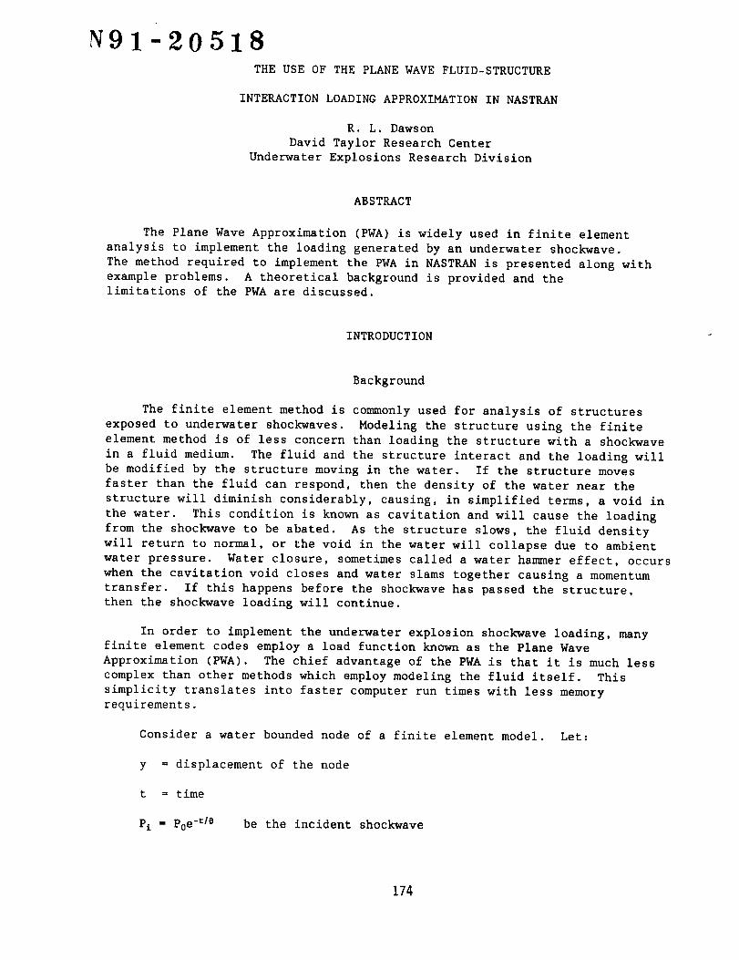
N91-20518THE USE OF THE PLANE WAVE FLUID-STRUCTURE
INTERACTION LOADING APPROXIMATION IN NASTRAN
R. L. Dawson
David Taylor Research Center
Underwater Explosions Research Division
ABSTRACT
The Plane Wave Approximation (PWA) is widely used in finite element
analysis to implement the loading generated by an underwater shockwave.
The method required to implement the PWA in NASTRAN is presented along with
example problems. A theoretical background is provided and the
limitations of the PWA are discussed.
INTRODUCTION
Background
The finite element method is commonly used for analysis of structures
exposed to underwater shockwaves. Modeling the structure using the finite
element method is of less concern than loading the structure with a shockwave
in a fluid medium. The fluid and the structure interact and the loading will
be modified by the structure moving in the water. If the structure moves
faster than the fluid can respond, then the density of the water near the
structure will diminish considerably, causing, in simplified terms, a void in
the water. This condition is known as cavitation and will cause the loading
from the shockwave to be abated. As the structure slows, the fluid density
will return to normal, or the void in the water will collapse due to ambient
water pressure. Water closure, sometimes called a water hammer effect, occurs
when the cavitation void closes and water slams together causing a momentum
transfer. If this happens before the shockwave has passed the structure,
then the shockwave loading will continue.
In order to implement the underwater explosion shockwave loading, many
finite element codes employ a load function known as the Plane Wave
Approximation (PWA). The chief advantage of the PWA is that it is much less
complex than other methods which employ modeling the fluid itself. This
simplicity translates into faster computer run times with less memory
requirements.
Consider a water bounded node of a finite element model. Let:
y = displacement of the node
t = time
Pi = Po e-t;e be the incident shockwave
174
Pr = _(t) be the reflected pulse off the model
Pa = mass per unit area associated with each node
P0 = density of water
8 = time constant of pressure pulse (assumed exponential)
A = water surface area associated with each node
The equation of motion of the node is:
t
p_P = Poe o + ¢ ( t)(1)
Continuity at the surface of the node stipulates that:
c-m
PoC_ = po e e _ _(t)(2)
Eliminating _ using equations (i) and (2) results in:
t
Pa9 + PoC_ = 2Poe e(3)
The resulting force applied at the node is given by:
F( t) = APa]# = 2Po e-_ - Po A(4)
The above equations were originally derived by Taylor in 1941
(reference i). The solution is exact as long as the water does not cavitate.
The water may cavitate at the node or a short distance away from the node.
Cavitation at the node will happen when:
t
PoC9 _ 2P0 e-_(5)
The nodal force derived from the PWA can be stated by combining
equations (4) and (5).
0 ; PoC_ > 2Poe _F(t) = t ¢
[2Poe-°-PoC_]A ; poc_ < 2Po e--8
(6)
Objective
The objective of this paper is to demonstrate the use of the PWA for
underwater shockwave loading in COSMIC NASTRAN for transient analysis
problems.
175
IMPLEMENTATION OF PLANE WAVE APPROXIMATION IN NASTRAN
The PWA can be implemented in COSMIC NASTKAN without the use of the DMAP
option. The procedure is facilitated by the use of scalar points and extra
points, as these points will add neither mass nor stiffness to the finite
element model. Consider a scalar dashpot which is implemented by the CDAMP4
card. The dashpot is constrained to ground by leaving one of the coordinates
on the CDAMP4 card blank. This will allow the dashpot to function
independently of the structure which is being analyzed. The dashpot is given
the value of p0c and loaded with an exponential shockwave:
t
P( t) = 2Po e-_(7)
Equation (7) is best implemented with the TLOAD2 card. NASTRAN will not
handle an instantaneous acceleration; therefore, equation (7) must be ramped
initially to its peak value. The ramp is established with the TLOAD1 card
coupled with the TABLED1 card. A ramp of 10 time steps to peak value was
chosen using engineering judgment. The additional 10 time steps increased
execution time only marginally while allowing sufficient ramp time to use
the TLOAD2 card. Therefore, no attempt was made to fine tune the number of
time steps in the ramp further. The TLOAD2 card is made to start on the 10th
time step by using the DELAY card. The TLOADI and TLOAD2 card are executed
together with the DLOAD card as shown in figure i. From first principles, the
velocity of the scalar point is:
t
_ 2Po e-_ (8)
(t) ,calar pc. po c
The wet node, extra point, and scalar point are equated using the TF
card, as shown in figure 2. Each water bounded node must be assigned its own
unique scalar dashpot, extra point and TF card. The TF relation defines the
extra point velocity:
U(t) ex. pt. = _( _) scalal pt. -- 9(t) wee node (9)
The NONLIN3 card is used to actually load the finite element model.
Each wet node must have its own unique NONLIN3 card and corresponding TF
card. As shown in figure 2, the NONLIN3 relation is:
PoCA[u(t) ex. pt.] ; u(t) ex. pc. > 0 (i0)F (t )wet n°de = 0 ; u (t )ax. pt. _ 0
(6)).
By using equations (8), (9), and (i0) the PWA will result (see equation
F(t) wee node =2Poe -_ - PoCk(t) ; 6_(t)ex, pt. > 0
0 ; _(t)_x.p_. _ 0
(ii)
176
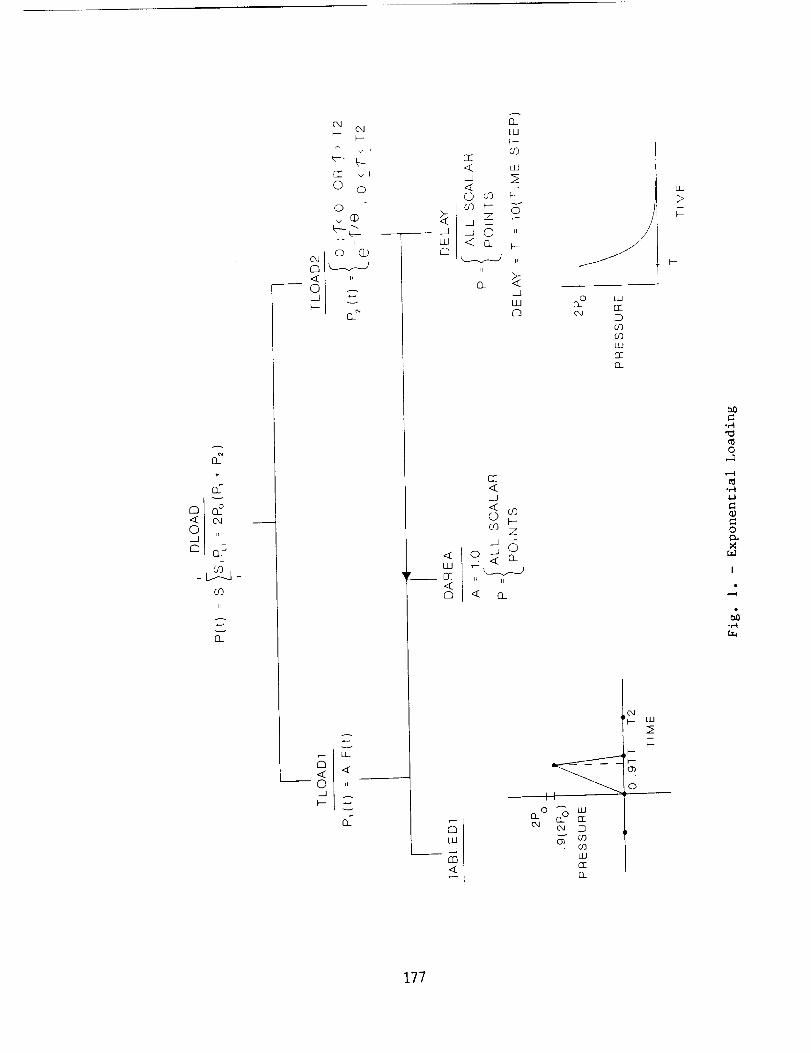
A
+
aT
L+0 ,_._J
O'3
11
n
c_c]
oJ
F-
[]Z v_
0 ©
©
v (D
+.
© (D
it
c"
c
LI-
J
aT
.<w
_CIZ<C]
.<
nLLI
F--CO
CIZ< LU
(D CO _-
.._i -J 0 "
0_LLJc]
cC.<
< oo
O3 Z
_]
H ii
"< n_
o uJ
cocoLUrrG_
"_ UJ
0
II
o_,,,n rr
cOUJrr
O_
LU
b_
o
,--I
o
I
.2
177
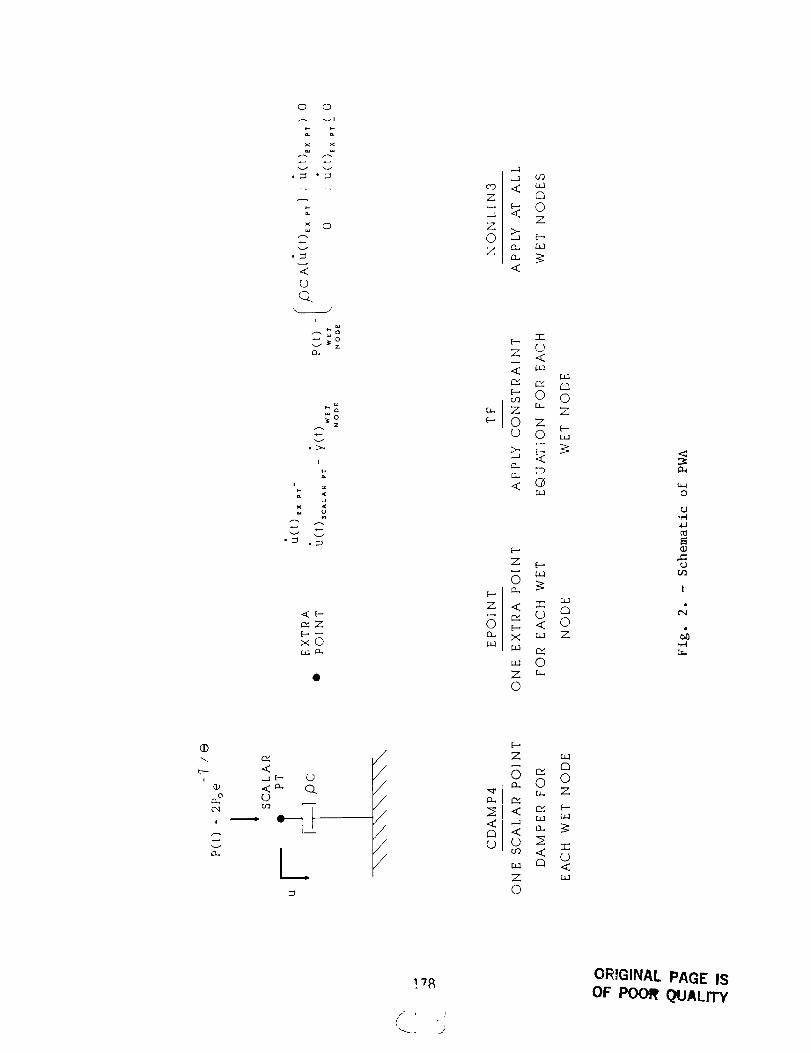
0 0
A vl
x x
• _ °_
w
<oQ
t-
_ov zCL
_o_z
I
dn0-
x
•g .g
<( [--.
xO
Q
,-.]
-_ ,_ ozz
<
Ib-
oz .<
r,1
_ c-< 123E- 0 0
_ z _' zb- 0 z __.
o 0 aa
r_
c_
< (?r_
b-
Z _
n ?:[---
0 E- '< 0x _ Z
0Z0
u_
0
¢J
03
I
¢
k----I
o
Ol
<_a _--. tO
<a. Q.o
L
Z uaC3
"_ r, Z
._, rv
t..l_l
o .r.
ua c_ <_z a_©
]78
t _"
",-.... _ ._.-)
ORIGINAL PAGE ISOF POOR QUALITY
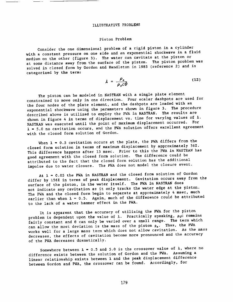
ILLUSTRATIVE PROBLEMS
Piston Problem
Consider the one dimensional problem of a rigid piston in a cylinder
with a constant pressure on one side and an exponential shockwave in a fluid
medium on the other (figure 3). The water can cavitate at the piston or
at some distance away from the surface of the piston. The piston problem was
solved in closed form by Gordon and Handleton in 1985 (reference 2) and is
categorized by the term:
i = . Pa (12)PoC8
The piston can be modeled in NASTRAN with a single plate element
constrained to move only in one direction. Four scalar dashpots are used for
the four nodes of the plate element, and the dashpots are loaded with an
exponential shockwave using the parameters shown in figure 3. The procedure
described above is utilized to employ the PWA in NASTRAN. The results are
shown in figure 4 in terms of displacement vs. time for varying values of i.
NASTRAN was executed until the point of maximum displacement occurred. For
= 5.0 no cavitation occurs, and the PWA solution offers excellent agreement
with the closed form solution of Gordon.
When _ = 0.5 cavitation occurs at the plate, the PWA differs from the
closed form solution in terms of maximum displacement by approximately 365.
This difference happens after 15 msec. Prior to this the PWA in NASTRAN has
good agreement with the closed form solution. The difference could beattributed to the fact that the closed form solution has the additional
impulse due to water closure. The PWA does not model the closure event.
At I = 0.05 the PWA in NASTRAN and the closed form solution of Gordon
differ by 156Z in terms of peak displacement. Cavitation occurs away from the
surface of the piston, in the water itself. The PWA in NASTRAN does
not indicate any cavitation as it only tracks the water edge at the piston.
The PWA and the closed form begin to separate at approximately 4 msec, much
earlier than when _ = 0.5. Again, much of the difference could be attributed
to the lack of a water hammer effect in the PWA.
It is apparent that the accuracy of utilizing the PWA for the piston
problem is dependent upon the value of I. Practically speaking, p0c remains
fairly constant and 8 can only be varied over a small range. The term which
can allow the most deviation is the mass of the piston Pa. Thus, the PWA
works well for a large mass term which does not allow cavitation. As the mass
decreases, the effects of cavitation become more pronounced and the accuracy
of the PWA decreases dramatically.
Somewhere between I = 0.5 and 5.0 is the crossover value of _, where no
difference exists between the solution of Gordon and the PWA. Assuming a
linear relationship exists between _ and the peak displacement difference
between Gordon and PWA, the crossover can be found. Accordingly, for
179
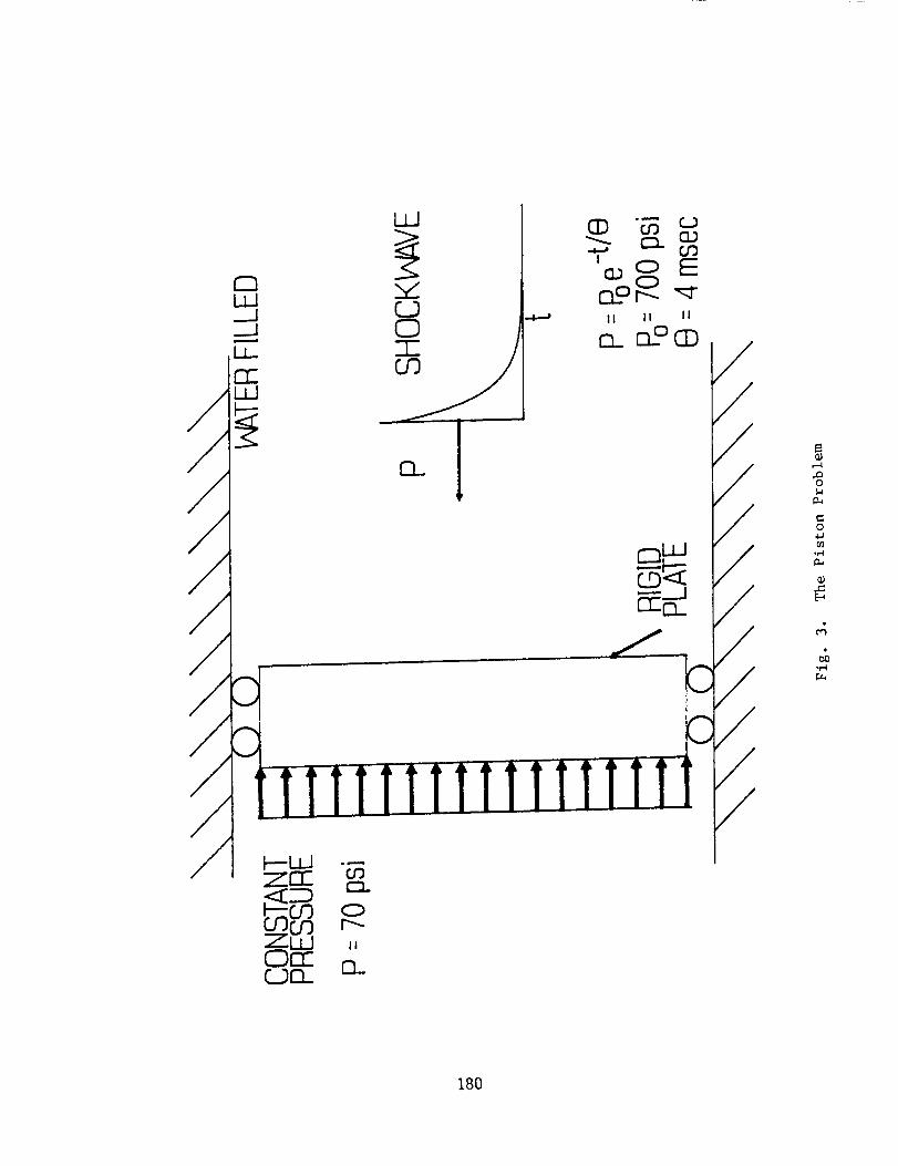
//////
C3_
..J
CIE
W
,,¢,Cb
°jJ
'_ EC1_or-...
II II II
CD_
//
////
/
o
o_J(Q
Q;
E_
// _---L.LJ .--
ZEIZ co
II
OQ_ n
180
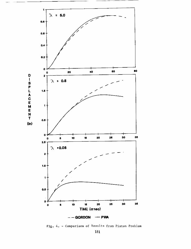
D
0.0
0.6
0.4
0.2
:5.0
t I20 40
t60 8O
I8PLACEMENT
(in)
1.6 "
0.5
0
0
2.6
1.5
0.6
"_ : 0.5
7J
f
ff
I
5 10 16 20
f
f
I I26 80
-0.05
35
f
J
fJ
/
//
/
I I6 10
I
0 I t i I
0 15 20 26 30
T;IL4F_/re'tee)
36
---GORDON --PWA
Fig. 4. - Comparison of Results from Piston Problem
181
= 0.64 and greater, no difference in displacement should exist between
PWA and the closed form solution of Gordon.
Circular Flat Plate With Mass
In this example a 2-inch thick flat circular plate is welded to a rigid
annular backing structure. The backing structure constrains the outside
of the plate but allows the inner section of the plate to move. In the center
of the plate a dummy mass is welded which weighs approximately the same
as the plate. The plate has air on one side, water on the other. A short
distance from the plate is an explosive charge which will release an
exponential shock'wave when detonated.
The experiment was conducted by the Underwater Explosions Research
Division of the David Taylor Research Center and is shown schematically in
figure 5. Velocity meters were placed on the mass to record the
experimental response.
A finite element model was formulated of the plate and mass using
COSMIC NASTRAN. Using symmetry, only a quarter of the plate was modeled using
plate elements. The mass was formulated using triangular plate elements and
the plate with quadrilateral elements. The plate was modeled as pin connected
at the edge. The mesh used is shown in figure 6. The PWA as described above
was used to load the model.
In this case the lowest value of I is 0.84. Although this problem is
very different than the piston problem, if the problems were analogous we
would expect no cavitation and the PWA to be an excellent method in which
to employ the underwater shockwave loading. The results from the NASTRAN
finite element model are plotted versus the experimental velocity in
figure 6. The analytical solution offers good agreement with experimental
results in terms of initial average acceleration, average deceleration and
peak velocity. These results support the use of the PWA for this application.
CONCLUDING REMARKS
The PWA is a useful engineering method for analyzing the shock response
of naval vessels from underwater explosions. The applicability of the method
is dependent upon the presence of cavitation in the water.
The PWA can be employed in NASTRAN for transient analysis problems
without using the DMAP option. Standard bulk data deck cards can be used.
The method requires the calculation for each wet node of several
parameters (A,P0,8) as well as an angular correction term if the shock-wave
and structure are not perpendicular. Additionally, several bulk data deck
cards will be needed for each wet node. An accounting system must be set up
in order to tie together the correct bulk data deck cards to the proper wet
node. If the finite element model is of sufficient size then accomplishing
182
J
Z
r-v _ f.--'_
JCI_
L_U
(I0
m i i
>
r-_c_
r'_X -I-
]
I
Zr-'l
I-iI..l
[--t
I
183
W
0=m
.q.e
*o t
°le°°***II*°°
W- =E
F,.
to'o*
h
Wa0=m
,,I
I._J
ZW=KI
mmWm_xW
Q_
Q.}
X
0
m<
0
0
o_._
1
9
184

the above can be quite a labor intensive task. A preprocessor program, which
could scan the NASTRAN input deck and output the required bulk data deck
cards necessary to implement the PWA, is recommended.
185

REFERENCES
i. Taylor, G. I., "The Pressure and Impulse of Submarine Explosion Waves on
Plates," Underwater Explosion Research, volume i, Office of Naval
Research, 1950. _--
2. Handleton, R. and Gordon, J., "Energy Absorption at a Restrained Mass,"
David W. Taylor Naval Ship Research and Development Center reportSD-85-24, March 1985.
186
N91-20519Sensitivity Analysis and Optimization Issues in NASTRAN
V. A. Tischler and V. B. Venkayya
ABSTRACT
Structural optimization in the context of integrated design is of
serious interest in many areas of engineering. In fact most of the commercial
finite element analysis software developers around the world are allocating
significant resources for implementing optimization in their programs. For
example the recent version of MSC/NASTRAN contains an optimization option in
addition to the sensitivity analysis which has been available for a number of
years. Sensitivity analysis is one of the key elements, and it must precede
the implementation of optimization. The purpose of this paper is to develop
procedures to extract sensitivity analysis information from COSMIC/NASTRAN and
to couple it with a mathematical optimization package. At present the
analysis will be limited to stress, displacement and frequency constraints
with structures modeled with membrane elements (such as QDMEMI, QDMEM2, and
SHEAR), rods and bar elements. Sensitivity analysis with the QUAD4 will be
addressed at a later date. The variables in sensitivity analysis are the
physical variables such as plate thicknesses, rod areas, etc. The approach
for sensitivity analysis is a combination of extracting information from
NASTRAN via DMAP and using subroutines written externally to NASTRAN. Two
types of sensitivity analysis will be addressed in this discussion. The first
is an adjoint variable approach which is most effective when the number of
active constraints is significantly less than the number of physical
variables. The second approach is based on a first order approximation of a
Taylor series. The latter approach is more effective when the number of
independent design variables is significantly less than the number of active
constraints.
(Paper not available at Press Time)
187

Report Documentation Page_ :dee Admt_sl,i}lbc_ _
1. Report No.
NASA CP-3111
4. Title and Subtitle
Nineteenth NASTRAN -f_-
7. Author(s)
2. Government Accession No.
Users' Colloquium
9. Pedorming Organization Name and Address
COSMIC, NASA's Computer Software Management andInformation Center
The University of Cmorgia
Athens, GA 30602
12. Sponsoring Agency Name and Address
Nati_na] Aeronautics and Space Administration
Washington, IX7 20546
3. Recipient's Catalog No.
5. Report Date
April 1991
6. Performing Organization Code
8. Performing Organization Report No.
10. Work Unit No.
11. Contract or Grant No.
13. Type of Report and Period Covered
Conference I_iblicat _on
14. Sponsoring Agency Code
15. Supplementary Notes
Also available from COSMIC, Athens, CA 30602
16. Abstract
This publication contains the proceedings of the Nineteenth NASTRANUsers'
Colloquium held in Williamsburg, Va., April 22-26, 1991. It provides
some comprehensive general papers on the application of finite elements in
engineering, comparisons with other approaches, unique applications, pre-
and postprocessing or auxiliary programs, and new methods of analysis withNASTRAN.
17. Key Words (Suggested by Author(s)}
NASTRAN, sttqlctures, structural
analysis, finite e]ement ana]ysis,
col loquium
18. Distribution Statement
Unclassified - Unlimited
Subject Category 39
19. Security Classif. (of this report) 20. Security Classif. (of this page) 21. No. of pages 22. Price
Unclassi fied Uncl assi lied 19 2 A09
NASA FORM 1626OCT 86Available from the National Technical Information Service,
Springfield, VA 22161 NASA-L&ngIey, 19@1
PRECEDING PAGE BLANK NOT FILMED

Related Documents