TRACTION MODELLING FOR A TOROIDAL CVT 18-month project for TOROTRAK (DEVELOPMENT) LTD Technical Report (TOR-4/02) by George K. Nikas Research Associate IC Consultants Ltd College House, 47 Prince’s Gate, Exhibition Road, London, SW7 2QA (in association with Imperial College of Science, Technology and Medicine, London, SW7 2AZ) April 2002

Welcome message from author
This document is posted to help you gain knowledge. Please leave a comment to let me know what you think about it! Share it to your friends and learn new things together.
Transcript

TRACTION MODELLING FOR A TOROIDAL CVT
18-month project for
TOROTRAK (DEVELOPMENT) LTD
Technical Report
(TOR-4/02)
by
George K. Nikas
Research Associate
IC Consultants Ltd
College House, 47 Prince’s Gate, Exhibition Road, London, SW7 2QA
(in association with Imperial College of Science, Technology and Medicine, London, SW7 2AZ)
April 2002

Contents 2
CONTENTS
ACKNOWLEDGEMENTS 2
LIST OF FIGURES 4
LIST OF TABLES 6
LIST OF SYMBOLS 7
1. Introduction 11
2. Mathematical analysis 13
2.1 Contact geometry and kinematics 13
2.2 Development of a generalized Reynolds equation 15
2.3 Fluid rheology 18
2.4 Film thickness 22
2.5 Boundary conditions 25
2.6 Numerical solution of the Reynolds equation 26
2.7 Subsurface stress analysis 28
2.8 Fatigue life model 30
2.8.1 Deformation Energy (Mises) criterion 32
2.8.2 Maximum Shear Stress criterion 32
2.9 Traction coefficient and contact efficiency 33
3. Application and parametric study 35
4. Application of the model on a test case 47
5. Effect of residual stresses 59
6. Conclusions 62
7. Computer program TORO (version 2.0.0) 64
7.1 Random Access Memory (RAM) and virtual memory (disk space) use 64
7.2 Program execution (CPU) time 65
7.3 Editing rules 65
7.4 Comments about roughness and transient effects 66
7.5 Input and output files 67
REFERENCES 75

Acknowledgments 3
ACKNOWLEDGEMENTS
The author is grateful to Dr Ritchie Sayles (Imperial College, Mechanical
Engineering Department, Tribology Section) for organising this project through IC
Consultants Ltd and appointing the author as the researcher.
The author wishes to thank Dr Jonathan Newall (Torotrak (Development)
Ltd), who was the industrial supervisor in this project, for his collaboration and help.
Thanks are also due to Dr Adrian Lee (Torotrak (Development) Ltd) for his help and
support. The author is grateful to Mr Mervyn Patterson, Dr Jonathan Newall, and Dr
Adrian Lee (Torotrak (Development) Ltd) for their review and comments on the
author’s 2002 paper related to this and previous work for Torotrak.
Finally, the author is grateful to Dr David Nicolson (Torotrak (Development)
Ltd) for initiating the project and dealing with the bureaucracy of its acceptance for
funding by the Department of Trade and Industry (DTI).
This project was financially supported by Torotrak (Development) Ltd and by
the British Department of Trade and Industry (DTI) through the Foresight Vehicle
LINK programme.

List of figures 4
LIST OF FIGURES
Figure Description Page
1.1 The Torotrak variator. 11
2.1 Basic geometry and kinematics of the toroidal CVT variator. 14
2.2 Infinitesimal block of fluid at the roller-disk contact. 16
2.3 Example of CPU time and solution error based on the author’s
method of accelerating the subsurface stress calculations. 29
2.4 Acceleration achieved and solution error based on the author’s
method of accelerating the subsurface stress calculations. 30
3.1 Flow chart of the model. 36
3.2 Effect of contact load (smooth contact; variable: P). 38
3.3 Effect of slide-roll ratio (smooth contact with p0 = 1.5 GPa;
variable: ur). 40
3.4 Effect of ellipticity ratio (smooth contact; variable: ry,r). 42
3.5 Effect of surface roughness (p0 = 1.5 GPa). 44
3.6 Effect of traction fluid bulk temperature (smooth contact; p0 = 1.5
GPa). 46
4.1 Contact pressure. 48
4.2 Contour map of the film thickness. 49
4.3 Roller x-traction, r
zx . 49
4.4 Roller y-traction, r
zy . 50
4.5 Roller resultant traction, r. 51
4.6 Roller x-traction over limiting shear stress, L
r
zx . 51
4.7 Roller y-traction over limiting shear stress, L
r
zy . 52
4.8 Roller traction over limiting shear stress, Lr . 53
4.9 Normal stress xx, 5.5 m below the surface of the roller. 53
4.10 Normal stress yy, 5.5 m below the surface of the roller. 54
4.11 Normal stress zz, 5.5 m below the surface of the roller. 54
4.12 Shear stress zx, 5.5 m below the surface of the roller. 55

List of figures 5
Figure Description Page
4.13 Shear stress zy, 5.5 m below the surface of the roller. 55
4.14 Shear stress xy, 5.5 m below the surface of the roller. 56
4.15 Shear stress zx, 55.0 m below the surface of the roller. 57
4.16 Shear stress zy, 55.0 m below the surface of the roller. 57
4.17 “Mises” stress (Eq. 36), 55.0 m below the surface of the roller. 58
5.1 Example of contours of the disk life for residual stress
combinations MPa400 , MPa 800 , MPa 800 zyx . 60

List of Tables 6
LIST OF TABLES
Table Description Page
1 Santotrac 50 properties (pressures up to 0.1 GPa; source:
Monsanto Corp.) 35
2 Data used for the examples. 37
3
Virtual memory (hard disk space) and peak RAM use (values
inside parentheses) of program TORO (steady-state analysis,
smooth contacts).
64

List of symbols 7
LIST OF SYMBOLS
Symbol Description
a Pressure-viscosity coefficient.
A Proportionality constant.
c Exponent of the fatigue stress criterion.
cz,x, cz,y See Eqs. (11).
czz,x, czz,y See Eqs. (11).
c1, c2 Fluid constants in the fluid density formula – Eq. (15).
d See the first of Eqs. (14).
dz,x, dz,y See Eqs. (14).
dzz,x, dzz,y See Eqs. (14).
D Local distance of the contacting surfaces (dry conditions) – Eq. (26).
De Local surface elastic displacement – Eqs. (29) and (33).
dr
eD , De(roller) + De(disk)
Dp Asperity plastic normal displacement.
Dx, Dy Lengths of the contact ellipse semi-axes – Eqs. (3).
e Elliptic-integral argument.
e Weibull slope.
E Elastic modulus.
Ed, Er Elastic modulus of the disk and the roller.
Eeff Effective elastic modulus – Eq. (4).
E(e) Complete elliptic integral of the 1st kind – Eqs. (6).
E.I.T. Efficient Input Torque – Eqs. (45)-(46).
h Local film thickness – Eq. (28).
hc Central film thickness.
hmin Minimum film thickness.
H “Height” of the variator (see Fig. 2.1).
K(e) Complete elliptic integral of the 2nd kind (see Eqs. (6)).
L Fatigue life.
Lrel Relative fatigue life.
Md, Mr Disk and roller torque.

List of symbols 8
Symbol Description
p Local contact pressure.
pH Hydrostatic pressure – Eq. (38).
p0 Maximum Hertz pressure.
P Contact load.
r “Radius” of the variator (see Fig. 2.1).
rx,d, ry,d Radii of curvature of the toroidal disk – Eqs. (1).
rx,r, ry,r Radii of curvature of the roller.
Rx, Ry Effective radii of curvature – Eqs. (2).
s Shear rate (for the Elsharkawy-Hamrock model see Eq. (18)).
S Probability of survival.
Sr Slide-roll ratio, drdrr uuuuS 2
t Time.
u Fluid velocity component on Ox – Eqs. (10), also in Figs. 2.1 and 2.2.
ud Tangential velocity of the toroidal disk on Ox – Eq. (7) and Fig. 2.2.
ur Tangential velocity of the roller on Ox (see Fig. 2.2).
zu Normal elastic surface displacement.
p
zu See Eq. (30).
zx
zu See Eq. (31).
zy
zu
See Eq. (32).
Fluid velocity component on Oy – Eqs. (10), also in Figs. 2.1 and 2.2.
r Tangential velocity of the roller on Oy (see Fig. 2.2).
Vref Volume where |ref | > u.
V Volume where | | > u.
w Fluid velocity component on Oz.
Y Yield stress in simple compression.
ZR Viscosity-pressure index – Eq. (21).
Fluid constant (in Eq. (25)).
Fluid constant (in Eq. (25)).
Effective surface roughness – Eq. (27).
r, d Roller and disk surface roughness height.
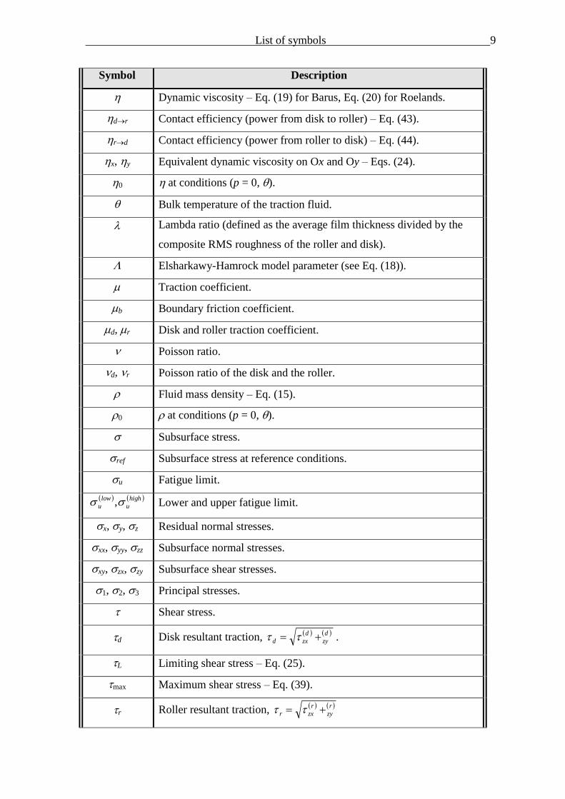
List of symbols 9
Symbol Description
Dynamic viscosity – Eq. (19) for Barus, Eq. (20) for Roelands.
dr Contact efficiency (power from disk to roller) – Eq. (43).
rd Contact efficiency (power from roller to disk) – Eq. (44).
x, y Equivalent dynamic viscosity on Ox and Oy – Eqs. (24).
0 at conditions (p = 0, ).
Bulk temperature of the traction fluid.
Lambda ratio (defined as the average film thickness divided by the
composite RMS roughness of the roller and disk).
Elsharkawy-Hamrock model parameter (see Eq. (18)).
Traction coefficient.
b Boundary friction coefficient.
d, r Disk and roller traction coefficient.
Poisson ratio.
d, r Poisson ratio of the disk and the roller.
Fluid mass density – Eq. (15).
0 at conditions (p = 0, ).
Subsurface stress.
ref Subsurface stress at reference conditions.
u Fatigue limit.
high
u
low
u , Lower and upper fatigue limit.
x, y, z Residual normal stresses.
xx, yy, zz Subsurface normal stresses.
xy, zx, zy Subsurface shear stresses.
1, 2, 3 Principal stresses.
Shear stress.
d Disk resultant traction, d
zy
d
zxd .
L Limiting shear stress – Eq. (25).
max Maximum shear stress – Eq. (39).
r Roller resultant traction, r
zy
r
zxr

List of symbols 10
Symbol Description
zx, zy Fluid shear stress components – Eqs. (17).
zyzx , Traction components.
d
zy
d
zx , Disk traction components.
r
zy
r
zx , Roller traction components.
0 Fluid constant (in Eq. (25)).
Roller angle (Fig. 2.1).
Angular velocity of the toroidal disk (see Fig. 2.1).
r Angular velocity of the roller.

§1. Introduction 11
1. Introduction
This project is a continuation of the author’s previous project for Torotrak,
which dealt with the modelling of the contact fatigue of the main components (rollers
and disks) of the variator of Torotrak’s Infinitely Variable Transmission (IVT). The
IVT variator is shown in Fig. 1.1.
Figure 1.1 The Torotrak variator.
Power is transmitted from an input toroidal disk through a roller to the output
toroidal disk and on to the drive shaft. The contact between a roller and a toroidal disk
is elliptical and the typical length of the axes of the contact ellipse is between 2 – 4
mm. The contacting surfaces are separated by a thin film of a special traction fluid,
with typical average thickness in the order of 0.5 m. The success of the transmission
is wholly dependent on the operation of these small contacts between the rollers and
the disks, which must sustain high loads and shear rates throughout the useful life of
Input toroidal disks
(powered by the engine)
Output toroidal disk
(transmits the power
to the drive shaft)
Rollers
(transfer power
from an input to
an output disk)

§1. Introduction 12
the transmission. Furthermore, the traction fluid plays the major role in keeping the
contacting surfaces separated, minimising wear but, at the same time, maximising the
traction force transferred from a roller to a disk or vice versa. The interrelationship of
these variables is complex and demands understanding and modelling of the fluid
rheology and the contact mechanics to a high degree and with as few simplifications
as possible.
The objective of the current project is the modelling of the traction and contact
efficiency of a typical roller-disk contact of the IVT variator, as well as the
subsequent evaluation (or prediction) of the life expectancy of the main components,
based on the analysis of the contact mechanics and elastohydrodynamics. For this
purpose, a generalized Reynolds equation was developed for the transient and non-
Newtonian lubrication of elliptical rolling-sliding-spinning rough contacts for the
specific kinematics of the toroidal IVT. The elastohydrodynamic analysis is
accompanied by a subsurface stress analysis (based on the computed contact pressure
and traction), which includes any residual stress fields, and the stress results are fed to
a fatigue life model (Ioannides-Harris) to compute the useful life of the main
components (i.e., the rollers and disks).
The traction and contact fatigue modelling is used as a tool to study the effect
of various parameters (contact load, fluid temperature, contact geometry, etc) on the
traction, efficiency and fatigue life of the variator components. Moreover, at the end
of this report, the effect of residual stresses on fatigue life is analysed and the
optimum residual stress fields to maximise the life expectancy are computed for a
specific application.
In the next pages, a full description of the mathematical and numerical model
is presented together with a parametric study and application through realistic
examples. Finally, the computer program developed for this project is presented near
the end of this report together with user instructions.

§2.1 Contact geometry and kinematics 13
2. Mathematical analysis
Unlike toothed transmissions, toroidal CVTs are traction drives and rely on
thin oil films to transmit power. These thin oil films must perform a very difficult task
under high stress and shear rate conditions, often operating in the mixed lubrication
regime and with complex kinematics that involve rolling, 2-dimensional sliding on the
tangent plane of the contact, as well as spinning, with, usually, contact velocities
changing in fast transient fashion during engine acceleration or variable torque
demands.
A collective presentation of the requirements and design criteria for IVTs can
be found in Patterson (1991) and although the literature contains a few papers on
traction studies for spinning elliptical contacts (as in Ehret et al. (2000) and Zou et al.
(1999)), these papers are not orientated to the specific kinematics of a toroidal CVT.
Moreover, the author is currently not aware of any papers dealing with the fatigue life
modelling of toroidal CVTs. The present study attempts to contribute in this field with
the development and application of a traction and fatigue-life model specifically for
toroidal CVT contacts, together with a parametric study of the main factors affecting
the life, traction and efficiency of such contacts.
2.1 Contact geometry and kinematics
The heart of a toroidal transmission is the variator, the basic function of which
is shown in Fig. 2.1. Power is transmitted from an input toroidal disk through a roller
to an output toroidal disk. Both the input and the output toroidal disks (hereafter
referred to as “disks”) rotate about axis AA. The roller rotates about axis BB and the
transmission ratio is altered continuously by varying the angle of the roller (Fig.
2.1). Lengths H and r are basic dimensions and are defined as the “height” and the
“radius” of the variator, respectively.
It is the elliptical contact between a roller and a disk that is simulated in the present
study. A coordinate system Oxyz is defined in Fig. 2.1, with point O being the
nominal point of contact, axis Oy parallel to BB and axis Ox perpendicular to the
page. The contact surfaces are approximated by ellipsoids with radii of curvature rx,r
and ry,r for the roller, and

§2.1 Contact geometry and kinematics 14
Fig. 2.1 Basic geometry and kinematics of the toroidal CVT variator.
sin
Hrrx,d , ry,d = r (1)
for the output disk. The effective radii of curvature, Rx and Ry are
sin1
,,
,,
H
rr
rr
rrR
dxrx
dxrx
x , ry
ry
dyry
dyry
yrr
rr
rr
rrR
,
,
,,
,,
(2)
The lengths Dx and Dy of the contact ellipse semi-axes are calculated by solving
numerically Eqs. (3):
2
3/1
2
2
1 ,
EKK1
E3
eDDeE
eeee
eRRP
D xy
eff
yx
x
(3)
where P is the contact load, Eeff is the effective modulus of elasticity of the roller and
disk
Output disk
Roller
Input disk
H
r
z
y,
x, u
O
A A
B
B

§2.2 Development of a generalized Reynolds equation 15
d
d
r
r
eff
EE
E22 11
1
(4)
(r and d being the Poisson ratios of the roller and the disk, respectively, and Er and
Ed being the elastic moduli of the roller and the disk, respectively), and e is calculated
numerically from
y
x
R
R
ee
eee
EK
K1E 2
, (Dx > Dy) (5)
where E(e) and K(e) are the 1st and 2nd-kind complete elliptic integrals of argument
e, respectively:
2/
0
22 sin1 E
dee ,
2/
0 22 sin1
1K
d-e
e (6)
The roller velocity on the tangent plane of the contact has a component ur on
the Ox axis (owing to its rotation about axis BB) and r on the Oy axis (owing to
changing angle ). The output-disk velocity is
sin rHud (7)
on the nominal point of contact on the Ox axis, where is the angular velocity of the
disk (Fig. 2.1).
2.2 Development of a generalized Reynolds equation
A typical toroidal CVT type contact operates under severe conditions of high
fluid local pressure and high shear rate. Both of the previous two conditions dictate
that the lubricant in such contacts behaves in a non-Newtonian manner most of the
time, i.e., the local internal shear stress of the lubricant in the contact is a non-linear
function of the local shear rate.
§2.2 Development of a generalized Reynolds equation 16
There are a number of non-Newtonian models in the literature that could be
used to describe the non-Newtonian behaviour of a lubricant under conditions of high
stress and shear rate. The accuracy of those models usually depends on the particular
lubricant to which they are applied as the actual rheology of lubricants is an area of
much debate in the literature due to the large number of physical parameters involved.
There is currently no generally accurate non-Newtonian model and, thus, a successful
model of the CVT lubrication must have room for different rheological laws to be
implemented and tested, depending on the traction fluids used and the operating
conditions. Therefore, a “generalized” lubrication (Reynolds) equation must be
developed, i.e., an equation that can readily incorporate different rheological models
in order to adapt to different lubricants and operating conditions and to discover
which rheological model best suits a particular application.
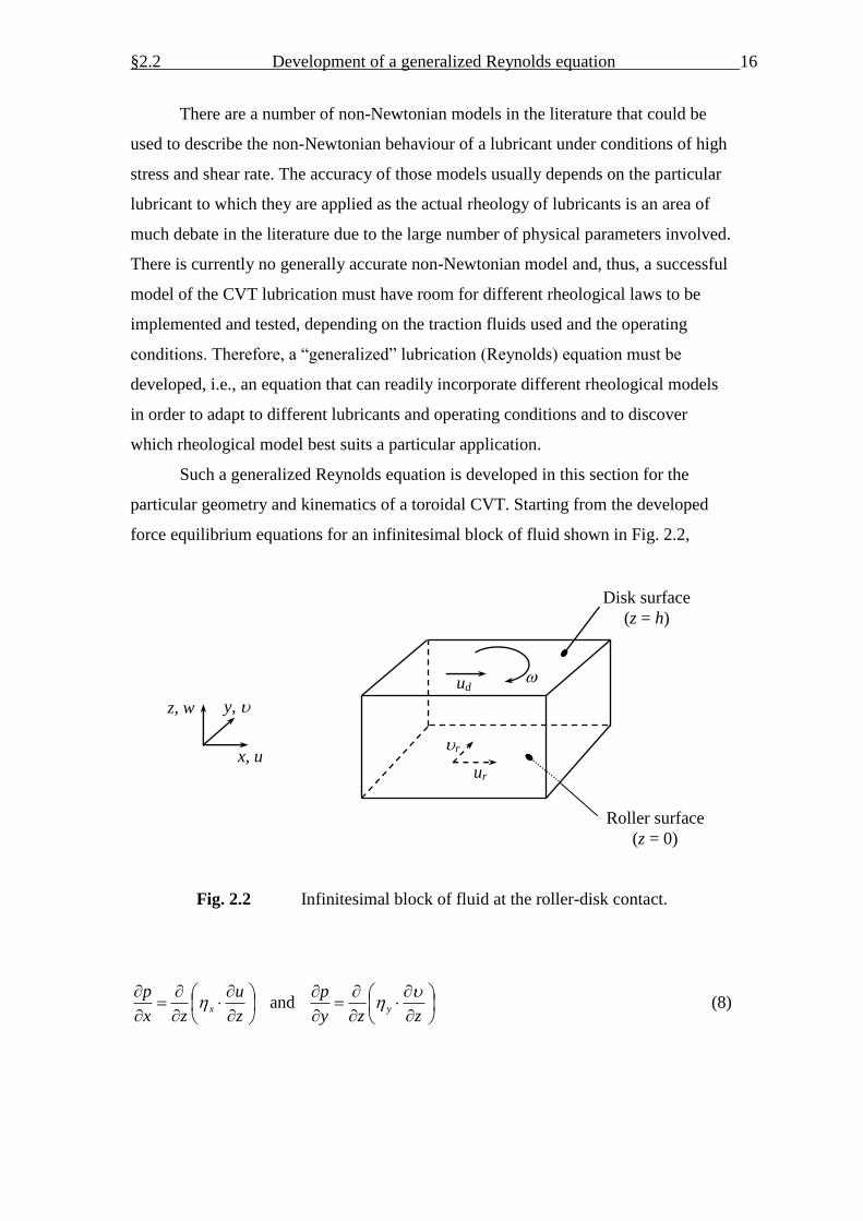
Such a generalized Reynolds equation is developed in this section for the
particular geometry and kinematics of a toroidal CVT. Starting from the developed
force equilibrium equations for an infinitesimal block of fluid shown in Fig. 2.2,
Fig. 2.2 Infinitesimal block of fluid at the roller-disk contact.
z
u
zx
px and
zzy
py
(8)
Disk surface
(z = h)
r
ud
ur
z, w y,
x, u
Roller surface
(z = 0)

§2.2 Development of a generalized Reynolds equation 17
where p is the fluid pressure and x and y are the equivalent fluid dynamic viscosities
in directions Ox and Oy, integrating with respect to z and using the “zero-slip”
conditions
xyrHuhz
uuz rr
, sin :
, :0
(9)
yields the fluid velocity components
zchc
x
y
pzc
hc
hczc
zchc
uyrH
x
pzc
hc
hczcuu
yz
yz
yz
yz
yzz
yzzr
xz
xz
rxz
xz
xzz
xzzr
,
,
,
,
,
,
,
,
,
,
,
,
sin
(10)
where
z
y
yzz
z
x
xzz
z
y
yz
z
x
xz
zdz
zczdz
zc
zdzczdzc
0 ,
0 ,
0 ,
0 ,
,
1 ,
1
(11)
and 0 z h, tyxhh ,, being the local film thickness (t stands for time).
Integrating the mass-conservation equation for the block of lubricant in Fig. 2.2
0
z
w
yx
u
t
(12)
( being the fluid mass density) with respect to z from z = 0 to z = h and after some
algebraic manipulation, the following lubrication equation is derived:

§2.3 Fluid rheology 18
0
sin
,
,
,
,
,
,
,
,
,
,
,
,
t
dd
hc
x
y
pd
hc
hcdd
y
dhc
uyrH
x
pd
hc
hcdud
x
yz
yz
ryz
yz
yzz
yzzr
xz
xz
rxz
xz
xzz
xzzr
(13)
where
h
yzzyzz
h
xzzxzz
h
yzyz
h
xzxz
h
dzzcddzzcd
dzzcddzzcd
dzd
0 ,,
0 ,,
0 ,,
0 ,,
0
,
,
(14)
and
pc
pc
2
101
1 (15)
according to Dowson and Higginson (1966) for mineral oils, where 0 is the fluid
density at ambient pressure and c1 and c2 are fluid constants. Equation (13) is a
generalized Reynolds equation, developed for the specific application of a toroidal
CVT (like the Torotrak IVT).
2.3 Fluid rheology
A number of rheological models are used in the present analysis, namely the
Newtonian model (but with a limiting shear stress constraint), and the non-Newtonian
models of Elsharkawy and Hamrock (1991), Bair and Winer (1979), and Gecim and
Winer (1980). For the results of this study presented later, the general Elsharkawy-
Hamrock model was used.

§2.3 Fluid rheology 19
Integrating the force equilibrium equations for a fluid element (as in Fig. 2.2)
zx
p zx
,
zy
p zy
(16)
with respect to z in the region [0, z], the fluid shear stresses zx and zy are derived:
y
pz
x
pz r
zyzy
r
zxzx
, (17)
where superscript “r” denotes the roller contact surface.
Using Eqs. (17), any non-Newtonian rheology model can be combined with
the generalized Reynolds Eq. (13). As an example, the Elsharkawy-Hamrock (1991)
model is used here, which can simulate other models via an adjustable parameter.
According to that model, the fluid shear stress and shear rate s are related as in
ΛΛ
L
s1
1
(Elsharkawy-Hamrock, 1991) (18)
where is the fluid dynamic viscosity, L is the limiting shear stress, and is an
adjustable parameter (positive integer) used to modify the behaviour of the
rheological model and simulate other models.
There are two widely used formulas in the literature for the dynamic viscosity
of a fluid: the one proposed by Barus (1893) and the one proposed by Roelands
(1966). The classical Barus’ formula reads as follows:
pae 0 (19)
where 0 is the dynamic viscosity at p = 0 (ambient pressure) and at the fluid
operating temperature, and a is the pressure-viscosity coefficient of the lubricant,
which depends on temperature. It has been experimentally found that for most
lubricants, Eq. (19) gives acceptable results for pressures up to 0.1 GPa but becomes

§2.3 Fluid rheology 20
progressively inaccurate for higher pressures. For pressures over 1 GPa, Eq. (19)
gives unacceptably high viscosity. A generally better equation was proposed by
Roelands (1966) following experimental work. Roelands’ semi-empirical formula,
which additionally accounts readily for the effect of temperature on the viscosity,
reads as follows (SI units only):
1101.5167.9ln exp 9
00 RZp (SI units) (20)
where ZR is the “viscosity-pressure” index, which is related to the pressure-viscosity
coefficient a of the Barus’ formula (Eq. (19)) as follows:
668.9ln101.5 0
9
aZR (SI units) (21)
The derivation of Eq. (21) is based on the assumption that the Roelands’ and Barus’
formulas must predict the same viscosity as the absolute pressure tends to zero.
Equations (20) and (21) agree well for low pressures but deviate substantially
for pressures over 1 GPa (the difference in the viscosity being several orders of
magnitude, depending on the lubricant – see for example Figure 4.4 in Hamrock
(1994)). The author’s model for this project allows the use of both the Barus and the
Roelands viscosity formulas as both have been pre-defined in the associated computer
program.
Returning to the rheological analysis now, the shear rates of the lubricant in
the contact are zus for direction Ox and zs for direction Oy. Therefore,
using Eq. (18),
ΛΛ
L
zy
zy
ΛΛ
L
zx
zx
zz
u/1 /1
1
,
1
(22)
Integrating Eqs. (22) with respect to z across the film and using Eqs. (17) gives

§2.3 Fluid rheology 21
r
h
ΛΛ
r
zy
L
r
zy
r
h
ΛΛ
r
zx
L
r
zx
xdz
y
pz
y
pz
uyrHdz
x
pz
x
pz
0 /1
0 /1
11
sin
11
(23)
Equations (23) are then solved numerically for the unknown surface stresses r
zx and
r
zy at each point (x, y) of the contact for the up-to-date film thickness h(x, y) and
pressure p(x, y) in a loop until convergence and agreement between pressure and film
thickness is achieved.
Having computed the surface shear stresses on the roller, r
zx and r
zy , shear
stresses everywhere across the film are easily computed from Eqs. (17). Then, the
equivalent viscosities x and y are calculated from
z
uzx
x
and
z
zy
y
(24)
using Eqs. (10) for the fluid velocity components.
The local shear stress in the fluid has an upper limit L, which, generally, is a
function of pressure and temperature :
pL 0 (25)
where 0, and are fluid constants. The constraint L must hold everywhere in
the fluid at the contact region. Using the shear stress components, the constraint to be
satisfied is: 222
Lzyzx . If the computed shear stress components are such that the

§2.4 Film thickness 22
limiting shear stress constraint is violated, the problem is resolved as follows (see also
Eqs. (10)).
Case u >
If Lzx (computed) , then set Lzxzx (computed)(new) sgn (sgn(x) is the sign function of x;
sgn(x) = +1 if x > 0 and sgn(x) = 1 if x < 0) and 0(new) zy . Otherwise (if
Lzx (computed) ), set 2 (computed)2(computed)(new) sgn zxLzyzy and (computed)(new)
zxzx .
Case u <
If Lzy (computed) , then set Lzyzy (computed)(new) sgn and 0(new) zx . Otherwise
( Lzy (computed) ), set 2 (computed)2(computed)(new) sgn zyLzxzx and (computed)(new)
zyzy .
Case u =
The shear stress components must be equal. Thus: 2sgn (computed)(new)
Lzxzx and
2sgn (computed)(new)
Lzyzy .
2.4 Film thickness
Approximating the smooth contacting surfaces by ellipsoids, their distance D
in dry conditions is calculated from
2222, yRxRRRyxD yxyx (26)
The surface roughness must be taken into account. The effective surface roughness
is the sum of the local roughness heights of the roller, r, and of the disk, d. During
operation, local asperity interactions may cause plastic deformation of individual
asperities, in which case the surface topography must be modified in real time. Thus,
the roughness term must include any plastic normal displacements Dp (Dp is
discussed in No. 5 of §2.5):

§2.4 Film thickness 23
tyxDyxyxtyx pdr ,,,,,, (27)
The local film thickness is then calculated from
0,0,0,0,),()0,0(),( ,, dr
e
dr
e DyxDyxyxDhyxh (28)
where dr
eD , is the sum of the normal elastic displacements of the contacting surfaces.
The transient normal elastic surface displacement De, owing to the contact
pressure and traction fields in the CVT contact, is, generally, calculated from
ellipse contact
2 2
2 2
2
,,
2
112
,1
,
dd
yx
yx
E
yx
p
E
yxD
zyzx
e (29)
being the Poisson ratio and E the elastic modulus. To avoid the discontinuity of the
integrand at points (x = , y = ) and the large amount of computing time required for
the double integral in Eq. (29) (hundreds of thousands of integrations must be
performed at each time step and for each convergence loop of the algorithm of the
problem), a faster method was followed; each surface is partitioned in elemental
rectangles of dimensions 2·x2·y. The elastic surface normal displacement at a
point (x, y) due to a uniform pressure over a rectangular area 2·x2·y is calculated
from (Eq. (3.25) in Johnson (1985))

§2.4 Film thickness 24
22
22
22
22
22
22
22
22
2
ln
ln
ln
ln
1
xxyyxx
xxyyxxyy
xxyyyy
xxyyyyxx
xxyyxx
xxyyxxyy
xxyyyy
xxyyyyxx
pE
u p
z
(30)
Most published studies tend to ignore the contribution of the tractions on the
surface displacements (and thus on the film thickness), but this introduces some error,
especially in rough contacts operating in the mixed lubrication regime. In a similar
manner that Eq. (30) was developed, the author developed equations for the elastic
surface normal displacement at a point (x, y) due to a uniform traction over a
rectangular area 2·x2·y:
2 2
2 2
2 2
2 2
ln
ln
2
1
arctanarctan
arctanarctan
2
112
yyxx
yyxxyy
yyxx
yyxxyy
xx
yy
xx
yyxx
xx
yy
xx
yyxx
Eu zxz
zx
(31)

§2.5 Boundary conditions 25
2 2
2 2
2 2
2 2
ln
ln
2
1
arctanarctan
arctanarctan
2
112
yyxx
yyxxxx
yyxx
yyxxxx
yy
xx
yy
xxyy
yy
xx
yy
xxyy
Eu zxz
zy
(32)
The normal elastic surface displacement is then the sum of the contributions of
all surface stress elements:
elements surface All
, zyzx
zz
p
ze uuuyxD
(33)
2.5 Boundary conditions
The boundary conditions of the problem are as follows.
1. The zero-slip conditions of Eqs. (9).
2. The cavitation condition: 0p .
3. Supported load = transmitted load: tPdydxtyxp
,, .
4. At areas of solid contact (if any), the surface shear stress is the product of the
pressure and the boundary friction coefficient b:

§2.6 Numerical solution of the Reynolds equation 26
r
zy
d
zy
r
zx
d
zx
rb
r
zy
rb
r
zx
xp
yrHup
h
,
sgn
sinsgn
0
5. If the computed local pressure exceeds the plasticity limit of 1.6·Y (Y being the
yield stress in simple compression), then that local pressure is set equal to the
limit: “ YpYp 6.1set then6.1 If ”. If the plasticity limit is exceeded in
an asperity contact, asperities are assumed to retract until the resulting
pressure relief brings the local pressure back on the plasticity limit. The
plastically displaced material is accommodated by small radial displacements
away from the contact point in such a way that the macroscopic dimensions of
the relevant body change imperceptibly. In this way, the plasticity term Dp
needed in Eq. (27) can be computed. This constraint of asperity plasticity is
based on both the Tresca and the Mises yield criteria for solids of revolution
(see Eqs. (6.8) and (6.9) in Johnson (1985)) and is applied to isolated
asperities with surface slopes less than 10, which is equivalent to the
application of Johnson’s cavity model (§6.3 in Johnson (1985)), as is
explained on p. 646 in Sayles (1996) and has been applied extensively by
Sayles and co-workers (among others). It is noted that this is used as a
reasonable approximation for isolated asperity contacts in order to avoid
unrealistic local stress peaks. Extended asperity contacts and asperity
“persistence” effects are out of the scope of this study and have no effect on
the results presented later.
2.6 Numerical solution of the Reynolds equation
Before the Reynolds Eq. (13) can be solved numerically, it must be made
dimensionless. The following dimensionless variables are defined.
Dimensionless pressure: 0p
p (p0 being the maximum Hertz pressure of the
contact).

§2.6 Numerical solution of the Reynolds equation 27
Dimensionless film thickness: yx DD
h
.
Dimensionless coordinates: xD
x,
yD
y,
yx DD
z
.
Dimensionless density: 0
.
Dimensionless dynamic viscosities: 0
x and 0
y.
Dimensionless time:
tDD
DDuu
yx
yxrdr
.
The dimensionless Reynolds equation was discretized using 2nd-order finite
differences and, usually, between 10010010 and 20020010 (x, y, z) gridpoints,
covering the area {–1.5·Dx x 1.5·Dx and –1.5·Dy y 1.5·Dy}. The resulting
difference equation is solved via the Successive Overrelaxation (SOR) method with
Chebyshev acceleration (see p. 860 in Press et al. (1992) for a suitable algorithm of
the SOR method). It must be emphasized here that the convergence rate of the
author’s algorithm is fast for maximum Hertz pressures up to 2 GPa and smooth
contacts, but becomes gradually worse at higher pressures and rough contacts.
Although the typical loading range of toroidal CVTs is between 1 and 2 GPa, higher
pressures up to 3 GPa are usually accounted for in a CVT design analysis. However,
such higher pressures are outside the normal operating range and, as shown later in
the examples, they cause a dramatic reduction of the fatigue lives of the rollers and
disks.
Computing times for the elastohydrodynamic (EHL) analysis are in the order
of 20 minutes (for the discretization of 20020010 gridpoints), using a 1.5 GHz
Pentium-4 PC. Although the SOR method is not as efficient as multigrid methods, it is
considered sufficient for the typical highly loaded cases of this study (maximum
pressures over 1 GPa) with low sliding and low spinning, all of which result in nearly
Hertzian contact pressure distributions.

§2.7 Subsurface stress analysis 28
2.7 Subsurface stress analysis
The computed contact pressure and traction fields are used as the boundary
loading for a 3-D subsurface elastic stress analysis using the general Boussinesq-
Cerruti equations (details given in §4 of the previous report of the author for Torotrak,
Nikas (1999)). The previous model has been enhanced in two areas: (a) to include
residual stresses in the analysis and (b) to accelerate the stress computations.
Regarding the residual stress inclusion, this was achieved by assuming a (x, y)
residual stress distribution on predetermined subsurface z-layers of both a roller and
the cooperating disk of the IVT variator. Each one of the six stress components of the
stress tensor was averaged on every one of the pre-determined z-layers and then fed to
the computer program for algebraic addition to the corresponding stress components
calculated through the normal EHD analysis.
Regarding the acceleration of the stress computations, it was achieved by a
simple method developed by the author, in which a number of gridpoints are excluded
from the computations based on a selection criterion. It must be emphasised here that
the EHD calculations normally account for no more than 1% of the total execution
(CPU) time of the computer program, when a subsurface stress analysis is performed.
Therefore, normally, over 99% of the CPU time is spent on subsurface stress
calculations. Typical examples of CPU times for a steady-state analysis, using the
minimum recommended number of gridpoints are as follows: 9 hours for a perfectly
smooth contact and 52 hours for a rough contact, using a 1.5 GHz Pentium-4 PC with
768 MB of 400 MHz RAM.
To reduce these excessive running times, the author developed a simple method to
assess the stress influence of one gridpoint over another and then selectively ignore
gridpoints whose stress influence is lower than a predetermined level. The method
includes a criterion to evaluate the error of a solution via a “residual” and, thus, make
accuracy comparisons with other solutions straightforward. Figure 2.3 shows a typical
example of the degree of acceleration achieved with the method described in the case
of a smooth contact.
The acceleration factor in Fig. 2.3 is chosen by the user of the author’s computer
program, based on the acceptable solution error (shown on the right vertical axis) in
combination with the “acceptably long” CPU time. As Fig. 2.3 shows, increasing the

§2.7 Subsurface stress analysis 29
0.0 0.4 0.8 1.2 1.60.2 0.6 1.0 1.4
Acceleration factor
0
0.02
0.04
0.06
0.01
0.03
0.05
0.07
So
luti
on
ave
rag
e r
esi
du
al
(err
or)
0
2
4
6
8
1
3
5
7
9
CP
U t
ime [
h]
1.5 GHz Pentium-4 PC, 768 MB of 400 MHz RAM Typical IVT example. Smooth contact.
Stress analysis: 303010 gridpoints. Subsurface stress calculated at 18000 gridpoints in total (9000 for each body).
solu
tion
erro
r
CPU time
Fig. 2.3 Example of CPU time and solution error based on the author’s
method of accelerating the subsurface stress calculations.
acceleration of the computations results in much shorter CPU time and greater
solution error. For zero solution error (no acceleration or full analysis), the CPU time
is 9 hours. Using an acceleration factor of 0.7, which gives satisfactory accuracy, the
CPU time is reduced to only 40 minutes, which represents an improvement of 1350%.
Even a modest acceleration factor of 0.1 will reduce the CPU time by 69% (2 hours
and 48 minutes instead of 9 hours).
The level of acceleration is clearer in Fig. 2.4, where the CPU-time has been
replaced by the number of times the execution of the computer program is accelerated
as a function of the acceleration factor. It can be seen that a 25-fold acceleration is
achievable by using an acceleration factor of 1.5.

§2.8 Fatigue life model 30
0.0 0.4 0.8 1.2 1.60.2 0.6 1.0 1.4
Acceleration factor
0
0.02
0.04
0.06
0.01
0.03
0.05
0.07
So
luti
on
ave
rag
e r
esi
du
al
(err
or)
1
5
9
13
17
21
25"
Tim
es
fast
er"
co
mp
are
d t
o t
he f
ull
so
luti
on
1.5 GHz Pentium-4 PC, 768 MB of 400 MHz RAM Typical IVT example. Smooth contact.
Stress analysis: 303010 gridpoints. Subsurface stress calculated at 18000 gridpoints in total (9000 for each body).
solu
tion
erro
r
acce
lera
tion
Fig. 2.4 Acceleration achieved and solution error based on the author’s
method of accelerating the subsurface stress calculations.
Figure 2.4 can also be used as a guide for rough surface analysis, where the
CPU times are much longer. For example, using an acceleration factor of 1.0, the
CPU time needed for a rough contact analysis was reduced from 52 hours to only 3
hours (precisely, 2 hours and 49 minutes), without a significant compromise in the
solution accuracy. This result is for a higher resolution of surface gridpoints, namely
980100 surface gridpoints for each body instead of 152100 points in the smooth-
contact case (6.4 times more gridpoints to account for the roughness effects).
2.8 Fatigue life model
For the obtained stress results, the Ioannides-Harris fatigue life model
(Ioannides and Harris (1985)) was applied with the depth weighting removed, as is
discussed and suggested in Lubrecht et al. (1990) and Tripp and Ioannides (1990).
According to this model, the fatigue life L (expressed in millions of stress cycles) and
the associated probability of survival S (0 < S < 1) are calculated from

§2.8 Fatigue life model 31
e
V
c
u dVA
SL
/1
1ln
,
V
c
u
e dVLAS
exp (34)
where stress is defined in Eq. (36), c is the stress-criterion exponent, u is the
fatigue limit, V is the volume of material where | | > u, e is the Weibull slope, and
A is a proportionality constant. What is of primary concern in this study is not the
absolute fatigue life L but the relative life, which is life L divided by a reference life,
both of which refer to the same probability of survival. The relative life, Lrel, is then
e
V
c
u
V
c
uref
rel
dV
dV
refLref
/1
(35)
where ref denotes the stress used for the reference life computation and Vref is the
volume of material where |ref | > u.
The fatigue limit is considered a random variable between a lower limit, low
u
and an upper limit, high
u , and depends on location. A pseudo-random number
generator is used to ascribe a fatigue limit to every point in the stress computational
grids, since every point represents an elemental volume of material with a constant
fatigue limit. This method gives effectively a Gaussian distribution of zyxu ,, .
Two fatigue-stress criteria are programmed in the model, namely the
Deformation Energy (Mises) criterion and the Maximum Shear Stress criterion. The
former is generally more accurate than the latter as it uses all six components of the
stress tensor and is more suitable for rough/asperity contacts with high local stress
concentrations; thus, it is the choice in the present study.

§2.8 Fatigue life model 32
2.8.1 Deformation Energy (Mises) criterion
According to the Mises criterion, the stress (or ref) to be used in Eqs. (34)
and (35) is calculated from
2
6 2222 2 2
yzxzxyxxzzzzyyyyxx
(36)
where xx, yy, zz, xy, xz and yz are the six components of the stress tensor.
2.8.2 Maximum Shear Stress criterion
According to the Maximum Shear Stress criterion, the stress (or ref) to be
used in Eqs. (34) and (35) is the maximum shear stress, corrected by the hydrostatic
stress:
Hp 3.0max (37)
where pH is the hydrostatic pressure
3
zzyyxx
Hp
(38)
and max is the maximum shear stress
2
,,min,,max 321321max
(39)
where 1, 2 and 3 are the principal stresses (as in §5.2 in Nikas (1999)), which are
functions of the six components of the stress tensor. The method to calculate the
principal stresses involves the solution of a cubic equation which must have three real
roots – the three principal stresses. However, due to numerical inaccuracies in the
computation of the stress tensor components, the solution of the said cubic equation is
problematic as it does not always result in three real roots (i.e., one of the computed

§2.9 Traction coefficient and contact efficiency 33
roots may be imaginary). To avoid this problem, the author assumed that the normal
stresses zzyyxx ,, are also the principal stresses, i.e., 1 = xx, 2 = yy, 3 = zz,
which is not expected to be far from true for the highly loaded CVT type contacts of
the present study. Using the previous assumption, stress of Eq. (37) is given from
zzyyxx
xxzzzzyyyyxx
1.0
2
,, max (40)
The endurance limit u for this criterion is defined as follows:
MPa9003.0 if 0
MPa9003.0 MPa600 if 3.0 88667.0798
MPa6003.0 if MPa 266
max
maxmax
max
H
HH
H
u
p
pp
p
(41)
2.9 Traction coefficient and contact efficiency
The traction coefficient is defined as follows:
P
dydxzx
(42)
where traction zx and the corresponding traction coefficient, , refer to either the
roller or the disk. For heavily loaded contacts like typical IVT type contacts, the area
where p > 0 (and so zx 0) is approximately the area of the contact ellipse; thus, the
numerical integration in Eq. (42) can be confined to the area of the contact ellipse.

§2.9 Traction coefficient and contact efficiency 34
The contact efficiency on the other hand is the ratio of the output power
divided by the input power. In the full toroidal IVT of Torotrak (Fig. 2.1), power is
transmitted from an input disk to a roller and from the roller to an output disk. Thus, a
roller receives power from a disk and transfers power to a disk. For these two types of
contact (“disk roller” and “roller disk”), contact efficiencies rd and dr are
given as follows:
rr
d
rr
ddr
uM
rrHP
M
M
sin (power from roller to disk) (43)
rM
uM
M
M
d
rr
d
rrrd
(power from disk to roller) (44)
where M stands for torque (with subscript “r” for the roller and with subscript “d” for
a disk), and r and d are the roller and disk traction coefficients, respectively.
For the results presented later, the input torque has been taken out of the
equation by defining a new variable named Efficient Input Torque (E.I.T. for short),
which is the product of the contact efficiency and the input torque. Thus:
r
ddrrdr
u
rrHPM
sinE.I.T. (power from roller to disk) (45)
rr
rddrd
uPM
E.I.T. (power from disk to roller) (46)
“E.I.T.” is a measure of how efficiently the input torque is used. For given (constant)
input torque, “E.I.T.” is proportional to the contact efficiency and, thus, the higher the
“E.I.T.”, the better.

§3. Application and parametric study 35
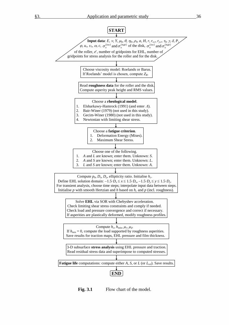
3. Application and parametric study
The model has been applied in a variety of cases covering the range of
operating conditions and design parameters used for Torotrak’s IVT. A simple flow
chart of the model is presented in Fig. 3.1. Application of the model in a 1.5 GHz
Pentium-4 PC with 786 MB of 400 MHz RAM require computation times of between
40 minutes and 3 hours for a steady-state analysis (EHL + subsurface stress analysis
and using the “acceleration factor” feature as explained in §2.7), depending on the
level of accuracy required. The results presented in this section refer to the power
transmission from a roller to an output disk.
The traction fluid used in the examples is Santotrac 50. The Roelands viscosity
formula (Eq. (20)) was used instead of the simpler but less accurate at high-pressure
formula of Barus (Eq. (19)). The dynamic viscosity, density and pressure-viscosity
coefficient are all functions of temperature and are shown in Table 1 for the range of
temperatures studied, although the test pressures for the data of Table 1 were much
lower than the maximum fluid pressures encountered in the examples.
Table 1
Santotrac 50 properties (pressures up to 0.1 GPa; source: Monsanto Corp.)
Temperature
[C]
0
[Pa·s]
0 *
[kg/m3]
a
[1/GPa]
50 0.0194 882 25.1
60 0.0131 875 22.8
70 0.0096 869 20.6
80 0.0073 863 19.1
90 0.0057 856 17.7
100 0.0046 850 16.5
* Density results derived with linear regression between 38 ºC and 93 ºC.
Data were not available for the viscosity-pressure index ZR of the Roelands formula
(Eq. (20)) and, thus, ZR is computed from Eq. (21), using the Barus pressure-viscosity
coefficient a given in Table 1.
§3. Application and parametric study 36
START
Input data: E, , Y, b, , 0, 0, a, H, r, rx,r, ry,r, 0, , , P,
, ur, r, , c, high
u
low
u and of the disk, high
u
low
u and
of the roller, e, number of gridpoints for EHL, number of
gridpoints for stress analysis for the roller and for the disk.
Choose viscosity model: Roelands or Barus.
If Roelands’ model is chosen, compute ZR.
Read roughness data for the roller and the disk.
Compute asperity peak height and RMS values.
Choose a rheological model.
1. Elsharkawy-Hamrock (1991) (and enter ).
2. Bair-Winer (1979) (not used in this study).
3. Gecim-Winer (1980) (not used in this study).
4. Newtonian with limiting shear stress.
Choose a fatigue criterion.
1. Deformation Energy (Mises).
2. Maximum Shear Stress.
Choose one of the following.
1. A and L are known; enter them. Unknown: S.
2. A and S are known; enter them. Unknown: L.
3. L and S are known; enter them. Unknown: A.
Compute p0, Dx, Dy, ellipticity ratio. Initialise hc.
Define EHL solution domain: 1.5·Dx x 1.5·Dx, 1.5·Dy y 1.5·Dy.
For transient analysis, choose time steps; interpolate input data between steps.
Initialise p with smooth Hertzian and h based on hc and p (incl. roughness).
Solve EHL via SOR with Chebyshev acceleration.
Check limiting shear stress constraints and comply if needed.
Check load and pressure convergence and correct if necessary.
If asperities are plastically deformed, modify roughness profiles.
Compute hc, hmin, r, d.
If hmin = 0, compute the load supported by roughness asperities.
Save results for traction maps, EHL pressure and film thickness.
3-D subsurface stress analysis using EHL pressure and traction.
Read residual stress data and superimpose to computed stresses.
Fatigue life computations: compute either A, S, or L (or Lrel). Save results.
END
Fig. 3.1 Flow chart of the model.

§3. Application and parametric study 37
Table 2 summarizes the input data used in the examples (power transmission
from roller to output disk).
Table 2
Data used for the examples.
“Height” of the variator (Fig. 2.1) H = 55 mm
“Radius” of the variator (Fig. 2.1) r = 50 mm
Radii of curvature of the roller rx,r = 50, ry,r = 30 mm
Angle (Fig. 2.1) = 0
Elastic modulus Er = Ed = 207 GPa
Poisson ratio r = d = 0.3
Roller velocity on Ox ur =10 m/s (except Fig. 3.3)
Roller velocity on Oy r = 0
Angular velocity of the disk (Fig. 2.1) = 176.4 rad/s (ud = 9.7 m/s)
Contact load P = 5000 N (except Fig. 3.2)
Operating temperature = 70 C (except Fig. 3.6)
Traction fluid Santotrac 50 (Table 1)
Fluid constants (in Eq. (15)) c1 = 0.6 GPa1
, c2 = 1.7 GPa1
Traction fluid limiting-shear-stress
constants (in Eq. (25))
0 = 317·105 Pa, = 0.093,
= 317 kPa/C
Rheological model and parameter Elsharkawy-Hamrock (1991), = 2
Stress-criterion exponent c = 31/3
Weibull slope e = 1.3
Fatigue limits high
u
low
u = 300 MPa
Boundary friction coefficient b = 0.1
The EHL problem was solved as explained in §7, using 20020010
gridpoints. The subsurface stress analysis and fatigue life analysis involved stress
computations with numerical grids of 303010 = 9000 points for each body, with
980100 gridpoints on each surface.

§3. Application and parametric study 38
The most important parameters on fatigue life, traction and contact efficiency
include the contact load (or maximum Hertz pressure), the slide-roll ratio, the bulk
temperature of the traction fluid, the contact ellipticity ratio, and the surface
roughness.
To begin with the parametric study, Fig. 3.2 shows the effect of the contact
load through the maximum Hertz pressure for a perfectly smooth contact.
0.8 1.2 1.61 1.4 1.8
Maximum Hertz pressure, p0 [GPa]
1
10
100
1000
10000
Re
lative
life L
rel (
ref:
p0 =
1.6
GP
a)
0
10
20
30
5
15
25
Effic
ient in
put to
rque (
E.I.T
.) [N
. m]
0.082
0.084
0.086
0.088
0.090
0.092
0.094
Dis
k tra
ction c
oeffic
ient,
d
0.40
0.60
0.80
0.45
0.50
0.55
0.65
0.70
0.75
0.85
0.90
0.95
Film
thic
kness [
m]
hc
hmin
Traction
Life
E.I.T
.
Hamrock-Dowson (Newtonian, no spin) - regression formulaPresent model (non-Newtonian, with spin) - actual data
Fig. 3.2 Effect of contact load (smooth contact; variable: P).
Starting with the film thickness results, the figure shows both the central film
thickness (hc, in the order of 0.8 m) and the minimum film thickness (hmin, in the
order of 0.5 m) computed through the present model as well as those derived from
the widely-used Hamrock-Dowson regression formulas for elliptical contacts (Eqs.
(22.18) and (22.20) in Hamrock, 1994). It is seen that there is close agreement for hc
between the present model and that of Hamrock-Dowson (the average difference is 26

§3. Application and parametric study 39
nm (1 nm = 103
m)), despite the fact that the Hamrock-Dowson model is for
Newtonian fluids and excludes spin, whereas the present analysis uses a non-
Newtonian model and includes spin. Close agreement between the two models is
observed for hmin, too (average difference of 20 nm). These small differences are
attributed to the applied rheological models for hc and to both the spin and rheology
effects for hmin. In comparison with the formulas proposed by Zou et al. (1999) for
elliptical contacts with spin but for Newtonian analysis, the results of the present
model are in agreement within 1% for hc and show an average difference of about 27
nm for hmin, explained by the effect of the non-Newtonian model with limiting shear
stress used in the present analysis as opposed to the classical Newtonian model
without limiting shear stress used in Zou et al. (1999).
Continuing with the results in Fig. 3.2, the load is increased six times from
1000 N to 6000 N, with the corresponding maximum Hertz pressure increasing 1.8
times from 0.9 GPa to 1.6 GPa. The disk traction coefficient is, predictably, increased
by about 12% but with decelerated rate at higher load. There is still a relatively high
level of traction (0.083) at the lightest load of the figure, namely at P = 1000 N (p0 =
0.9 GPa). Following the increase of traction d and load P, the Efficient Input Torque
(E.I.T.), which is proportional to d and P (Eq. (45)), is significantly increased and
with an accelerated rate. On the other hand, the lives of the roller and the disk (the two
curves are indistinguishable in the figure) are substantially reduced by about 5000
times because of the increased contact pressure. The results show that, although a load
increase is clearly beneficial in terms of traction and efficiency, it is particularly
detrimental for the fatigue life of the components. Thus, a compromise must be
reached between these three parameters. Notice that, although the results are for a
smooth contact, the computed minimum hmin is still sufficiently thick to guarantee full
film separation of the surfaces for typically rough IVT components (i.e., components
with average roughness of less than 0.2 m – this is discussed later).
Next, the effect of the slide-roll ratio drdrr uuuuS 2 is shown in
Fig. 3.3. The ratio was changed by changing only the roller speed ur.

§3. Application and parametric study 40
0.00 0.10 0.200.05 0.15
Slide-roll ratio, Sr
0.970
0.980
0.990
1.000
0.975
0.985
0.995
Re
lative
life
Lre
l (re
f: S
r =
0)
0
5
10
15
20
25
Effic
ient in
put to
rque (
E.I.T
.) [N
. m]
0.00
0.02
0.04
0.06
0.08
0.10
0.01
0.03
0.05
0.07
0.09
Dis
k tra
ction c
oeffic
ient,
d
0.2
0.4
0.6
0.8
1.0
0.3
0.5
0.7
0.9
Film
thic
kness [
m]
Hamrock-Dowson (Newtonian, no spin) - regression formulaPresent model (non-Newtonian, with spin) - actual data
Disk life
Roller life
Traction
hmin
hc
E.I.T.
Fig. 3.3 Effect of slide-roll ratio (smooth contact with p0 = 1.5 GPa; variable: ur).
Both hc and hmin are increased with Sr and, again, there is close agreement between the
present model and the Hamrock-Dowson formulas, with average differences of 29 nm
for hc and 31 nm for hmin. Using the formulas of Zou et al. (1999) that include spin
(but are for Newtonian analysis), the average differences with the present model are
less than 1% for hc and 36 nm for hmin. An interesting observation is made for the
author’s computed hmin in Fig. 3.3: it is generally slightly higher than that of the
Hamrock-Dowson formula, except for the region 0 < Sr < 0.05. For that region of low
slide-roll ratio, the effect of spin is dominant. Minimum hmin is computed for Sr
0.013. This is proved mathematically as follows: the local sliding velocity in the
rolling direction is yuu dr and becomes zero for yuu dr ; for an
average y = –Dy/2 = – 722.5·106
m (computed Dy = 1445 m), the local sliding
velocity becomes zero for ur = 9.7 + 0.127 = 9.827 m/s, which corresponds to Sr
0.013. The minimum film thickness “appears” only on one part of the contact, where

§3. Application and parametric study 41
the local sliding velocity is minimized (see for example Fig. 7 in Zou et al. (1999) as
well as Fig. 4.2 later in the present study).
Continuing with Fig. 3.3, the traction curve shows the classical behaviour of
isothermal EHL, being nearly zero at Sr = 0, rising sharply for Sr > 0 and, finally,
following a slow increase for Sr greater than a certain value. A similar result is shown
in Fig. 13 of Ehret et al. (2000) (theoretical study), in Fig. 7 of the experimental work
with a toroidal IVT variator of Newall et al. (2002), and in Fig. 2.1 of Patterson
(1991). The traction absolute value and trend have been verified in an MTM rig for
the same fluid as that used in the present study (Santotrac 50) in the author’s
laboratories (Anghel, 2002). Notice that, for Sr = 0, there is still some traction (d
0), because of the spin effect in the contact (for Sr = 0, the local sliding velocity is not
eliminated in the contact, except at the centre (x, y) = (0,0)).
The E.I.T. is now affected by d and ur (the only variables in Eq. (45)). For
low Sr (low ur), the dominant variable is d, hence E.I.T. follows closely the
behaviour of the traction curve. For higher Sr (higher ur), the roller speed ur becomes
the dominant factor and, when the traction coefficient d levels off, the continuing
linear increase of ur causes a nearly linear decrease of E.I.T., as Eq. (45) dictates.
Similar results of efficiency are shown in Figs. 7 and 8 of Ehret et al. (2000), as well
as in Fig. 5.1 of Patterson (1991) for traction drives.
Regarding the roller and the disk fatigue lives, these are clearly shown to
follow the behaviour of the traction curve. Using as a reference point the lives at Sr =
0, the lives are shown to, initially, decrease by 1.5% for the roller and 2.0% for the
disk because of the increased traction and associated higher shear stresses imposed on
the two components. It is also obvious that the life curves follow the initial reduction
of hmin at very low Sr, which was explained previously. As the traction levels off, so
do the fatigue lives. The figure shows that the life is marginally affected by the slide-
roll ratio at these conditions. The absolute minimum film thickness of about 0.29 m
would be sufficient to prevent asperity interactions if the components were
realistically rough, so roughness would not be expected to affect the results in this
case. Conclusively, Fig. 3.3 “suggests” that the optimum slide-roll ratio would be that
for which the efficiency is maximized, or slightly higher, if a bit more traction is
required. It is noted here that, although thermal effects would finally cause a reduction
of traction at high slide-roll ratio, this would not affect the present results because the

§3. Application and parametric study 42
maximum slide-roll ratio used in Fig. 3.3 is still small for thermal effects to become
dominant.
Moving on to another important design parameter, Fig. 3.4 shows the effect of
the ellipticity ratio of the contact.
0.8 1.2 1.61.0 1.4 1.8
Ellipticity ratio, Dy/Dx
0.0
0.4
0.8
1.2
1.6
2.0
0.2
0.6
1.0
1.4
1.8
Re
lative
life
Lre
l (re
f: D
y/D
x =
0.9
5)
22.0
22.4
22.8
23.2
22.2
22.6
23.0
23.4
Effic
ient in
put to
rque (
E.I.T
.) [N
. m]
0.0910
0.0920
0.0930
0.0940
0.0905
0.0915
0.0925
0.0935
Dis
k tra
ction c
oeffic
ient,
d
0.2
0.4
0.6
0.8
1.0
0.3
0.5
0.7
0.9
Film
thic
kness [
m]
0.0
1.0
2.0
3.0
0.5
1.5
2.5
Maxim
um
Hert
z p
ressure
, p
0 [G
Pa]
Tra
ction
Pressure
hc
hmin
Hamrock-Dowson (Newtonian, no spin) - regression formulaPresent model (non-Newtonian, with spin) - actual data
Life
E.I.T.
Fig. 3.4 Effect of ellipticity ratio (smooth contact; variable: ry,r).
The crown radius ry,r of the roller is the only independent variable in the figure (the
load is constant, P = 5000 N), varied between 24 and 34 mm, which effectively
changes the ellipticity ratio from about 0.9 to about 1.6. This results in an increase of
both the central and the minimum film thickness. Again the differences between the
film thickness predictions of this model and of the Hamrock-Dowson formulas is
small, as can be seen in Fig. 3.4 (the average difference is 21 nm for hc and 37 nm for
hmin; using the formulas of Zou et al. (1999), the average difference in hmin is 60 nm,
whereas the results for hc agree on average within 1%).
The disk traction curve shown in Fig. 3.4 shows a rather small but clear
reduction with the ellipticity ratio (d reduced from about 0.093 to about 0.091). The

§3. Application and parametric study 43
same result has been obtained experimentally in Newall et al. (2002) (Fig. 9 in that
paper), using an IVT variator test rig. Following the reduction of traction, the E.I.T.,
which is affected here only by d (see Eq. (45)), is showing a similar relatively small
reduction, which is straightforward to realize from Eq. (45). On the other hand, the
lives of the roller and the disk (the two curves being indistinguishable in the figure),
show a characteristic behaviour in that they are clearly maximized at an ellipticity
ratio slightly higher than 1 (at about 1.05). The life curve falls sharply for ellipticity
ratio less than 1 and more gently at ellipticity ratios over 1.05. These results are
proved mathematically as follows: life (see the first of Eqs. (34)) is inversely
proportional to the effective subsurface stress , which, for the Mises stress criterion,
is defined in Eq. (36). Assuming for a moment that there were no surface traction in
the contact, a circular contact (ellipticity ratio = 1) would have a subsurface stress
distribution of xx quite close to that of yy; that would minimize (see Eq. (36)),
because the term (xx – yy) would be nearly eliminated, which is certainly not the
case for ellipticity ratio different than 1. Thus, through the minimization of at
ellipticity ratio of 1, life would be maximized. Next, including traction in the
discussion, the only difference would be that at an ellipticity ratio of 1, xx would be
greater than yy due to the added contribution of traction (which is predominantly on
the Ox direction). Thus, in order to have yy xx, the ellipticity ratio must be slightly
higher than 1, which gives the additional potential for yy to approach xx and
minimize . Therefore, life should be maximized at an ellipticity ratio slightly higher
than 1 (hence the result of 1.05 in Fig. 3.4). On the other hand, to understand the
result for life at values of the ellipticity ratio other than ~1, one has to look at the
contact pressure curve included in Fig. 3.4. The sharp reduction of life for ellipticity
ratio below 1 is explained by the corresponding increase of the contact pressure,
whereas the reduced rate of reduction of life at ellipticity ratios above 1 is obviously
explained by the corresponding reduction of the contact pressure. The two factors
affecting life here are the symmetry (or asymmetry) of the subsurface stress field and
the contact pressure. Studying the main curves in Fig. 3.4, the conclusion is that the
optimum ellipticity ratio is “slightly higher than 1”: this would maximize life and
offer traction and efficiency performance close to their maximum, with a minimum
film thickness (of about 0.4 m) still adequate to avoid roughness asperity
interactions with realistically rough components.

§3. Application and parametric study 44
The effect of roughness is shown next in Fig. 3.5 for maximum Hertz pressure
p0 = 1.5 GPa.
0 0.1 0.2
RMS roughness (roller and disk) [m]
20000
40000
60000
80000
100000
10000
30000
50000
70000
90000
Re
lative
life
Lre
l (re
f: R
MS
= 0
.23
m
)
21.4
21.6
21.8
22.0
22.2
22.4
21.5
21.7
21.9
22.1
22.3
Effic
ient in
put to
rque (
E.I.T
.) [N
. m]
0.086
0.088
0.090
0.092
0.085
0.087
0.089
0.091
Dis
k tra
ction c
oeffic
ient,
d
0.0
0.2
0.4
0.6
0.1
0.3
0.5
0.7
Min
imum
film
thic
kness [
m]
4
8
12
16
20
2
6
10
14
18
Lam
bda r
atio, (
usin
g a
vera
ge film
thic
kness)Traction
E.I.T.
Disk life
Roller life
Film thickness
Lambda ratio
1
Fig. 3.5 Effect of surface roughness (p0 = 1.5 GPa).
The roughness profiles of the roller and the disk were generated mathematically using
a random number generator and varying the asperity heights in order to get the desired
RMS (Root Mean Square) roughness values, the latter being in the range of 0.0-0.2
m, which is the typical range for these IVT components. Starting with the minimum
film thickness result, Fig. 3.5 shows that hmin is reduced with RMS roughness, as
expected, until it becomes zero (first asperity contacts) at an RMS roughness of about
0.23 m. The lambda ratio (defined as the average film thickness in the contact
divided by the composite RMS roughness), which is shown in Fig. 3.5, becomes equal
to 2.4 at the point where hmin becomes zero.
The traction curve is not significantly affected by the RMS roughness until the
minimum film thickness is significantly reduced (to less than 0.1 m) for RMS > 0.15
m ( < 3); in that region and, especially when the first asperity collisions take place,
the traction coefficient shows a clear drop in the order of 0.002. The insensitivity of
traction to the roughness magnitude as long as there is full film separation of the

§3. Application and parametric study 45
surfaces was also concluded in, for example, Chang (1992) (see Conclusion 1 in that
paper) and in Evans and Johnson (1987) (see Conclusions on p. 149 of that paper).
Following the behaviour of the traction coefficient, the E.I.T. (which is
affected here only by d – see Eq. (45)) shows the same behaviour, with a relatively
small but abrupt reduction for RMS > 0.15 m, and this result is straightforward to
extract from Eq. (45). The insensitivity to the RMS roughness when there is full film
separation is even more clear to see on the life curves of the roller and the disk: those
curves are almost level until opposing roughness asperities of the two components
approach closely each other and eventually come into contact, in which case the life
drops dramatically by more than 70000 times. Such magnitude of life reduction has
also been derived theoretically by Tripp and Ioannides (1990) (see Fig. 2 in that
paper) in the study of the effect of roughness on rolling bearing life. Asperity
interactions create high localized stresses, which can exceed significantly the
maximum Hertz stress of the contact (up to the point of local material yield). At the
point where hmin becomes zero (shown in Fig. 3.5), the computed load supported by
roughness asperities is 1% of the contact load P. In conclusion, all results of Fig. 3.5
suggest that the effect of the magnitude of roughness (expressed through the RMS
value) on the traction coefficient, efficiency and fatigue life, is negligible for as long
as a full film separates the cooperating surfaces, which is the case for RMS roughness
< 0.15 m (or, equivalently, for > 3), in which region all of these variables are
maximized. Therefore, there is no obvious benefit in using “very” smooth
components.
Moving on to temperature effects now, the effect of the bulk temperature of
the traction fluid is shown in Fig. 3.6, referring to a perfectly smooth, heavily loaded
contact (p0 = 1.5 GPa). Starting with the film thickness results, it is clear that both the
central and the minimum film thickness are significantly reduced as the temperature is
increased from 50 C to 100 C. The average film thickness difference between the
present model and the Hamrock-Dowson formulas is 27 nm for hc and 116 nm for
hmin. Using the formulas of Zou et al. (1999) that include spin (but are for Newtonian
analysis), the average difference for hmin is 117 nm (attributed mainly to the
Newtonian versus non-Newtonian model with limiting shear stress used), whereas the
results for hc agree within 1% on average.

§3. Application and parametric study 46
60 80 10050 70 90
Traction fluid bulk temperature, [oC]
1.00
1.04
1.08
1.12
1.16
1.02
1.06
1.10
1.14
Re
lative
life
Lre
l (re
f:
= 5
0 o
C)
16
18
20
22
24
26
Effic
ient in
put to
rque (
E.I.T
.) [N
. m]
0.075
0.080
0.085
0.090
0.095
0.100
Dis
k tra
ction c
oeffic
ient,
d
0.0
0.4
0.8
1.2
1.6
0.2
0.6
1.0
1.4
1.8
Film
thic
kness [
m]
hc
hmin
Traction
Rolle
r lif
eD
isk
life
Hamrock-Dowson (Newtonian, no spin) - regression formulaPresent model (non-Newtonian, with spin) - actual data
E.I.T
.
Fig. 3.6 Effect of traction fluid bulk temperature (smooth contact; p0 = 1.5 GPa).
The traction coefficient shows a 20% reduction from 0.100 at 50 C to 0.080
at 100 C. This reduction follows of course the reduction of the viscosity of the
traction fluid, as shown in Table 1. As expected, the E.I.T. shows also a reduction, in
agreement with the reduction of d, which is the only variable in Eq. (45) in this case.
On the other hand, the lives of the roller and the disk show an increase, which is about
14% at the highest temperature of 100 C in the figure, in relation to the lives at 50
C. This life increase is caused by the reduced viscous shear stresses in the contact
zone, owing to the reduction of the fluid viscosity at elevated temperatures. However,
it is emphasized here that these results are for a perfectly smooth contact. In a
realistically rough contact, the reduction of the minimum film thickness shown in Fig.
3.6 may cause roughness asperities to engage in collisions, which would inevitably
cause a substantial reduction of the fatigue lives, as was demonstrated in Fig. 3.5. On

§4. Application of the model on a test case 47
the other hand, even for very smooth contacts, the possible presence of debris
particles in the fluid, in combination with the film thickness reduction at higher
temperature, could also cause surface distress, which would inevitably reduce the
fatigue life. Therefore, the predicted life increase of Fig. 3.6 during operation at
higher fluid temperature is valid for as long as there is full film separation of the
cooperating surfaces. Summarizing the results of Fig. 3.6, since both traction and
E.I.T. show a significant increase at lower temperature, accompanied by thicker films
that may help avoid any roughness asperity interaction and debris particle interference
in the lubrication of the contact, and since the components’ fatigue lives are not
significantly reduced at low temperature (and with the possibility to be substantially
reduced at high temperature from asperity and debris particle involvement due to the
film thickness reduction), it is concluded that the fluid bulk temperature is best to be
kept on the low side of the studied temperature range.
4. Application of the model on a test case
This section presents a full example of the application of the model for a
perfectly smooth contact at steady-state conditions. All details and input data for this
test case are the same as those presented in Tables 1 and 2. The elastohydrodynamic
lubrication problem (contact pressure, film thickness, traction) was solved
numerically, as explained in §2.6, using 10010010 (x, y, z) gridpoints. The
subsurface stress analysis was performed using 606010 (x, y, z) gridpoints (spatial
steps of about 3.3 m in the x-direction and 4.3 m in the y-direction) for each
component (72000 gridpoints in total), and the acceleration factor (explained in §2.7)
was chosen equal to 0.2, giving priority to computational accuracy rather than
program execution speed. The CPU time was 47 hours (almost 2 days) on a 1.5 GHz
Pentium-4 PC with 768 MB of 400 MHz RAM. Using the author’s computer program
TORO (version 2.0.0) for this study, here follow some important results.
Roelands viscosity-pressure index, ZR 0.80 (computed from Eq. (21)).
Maximum Hertz pressure, p0 = 1.5 GPa.
Contact ellipse semi-axes lengths, Dx 1101 m, Dy 1445 m.
Central film thickness, hc 0.775 m.
Minimum film thickness, hmin 0.494 m.

§4. Application of the model on a test case 48
Traction coefficients, r 0.0923 (roller) and d 0.0922 (disk).
Efficient Input Torque, E.I.T. 22.52 N·m.
On average in the contact, %00.89L
r
and %31.89
L
d
(where
r
zy
r
zxr is the resultant traction of the roller and d
zy
d
zxd is the
resultant traction of the disk).
On average in the contact,
%07.84L
r
zx
and
%43.84L
d
zx
.
The contact pressure distribution is shown in Fig. 4.1.
Fig. 4.1 Contact pressure.
The pressure distribution resembles the typical Hertzian pressure distribution of a dry
contact for it refers to a highly loaded contact (p0 = 1.5 GPa) with low sliding
(nominal sliding speed = 0.3 m/s) and low spinning. However, the effect of spin is
clear in the film thickness distribution. Figure 4.2 shows a contour map of the film
thickness in the contact. It is seen that the two zones of film thinning are at the
locations typical for sliding elliptical contacts, but the absolute minimum of the film
thickness appears at only one part of the contact, at the area where the local sliding
speed is minimized (in magnitude). That location is as shown with red colour at the

§4. Application of the model on a test case 49
lower half part of Fig. 4.2 (see also the comments below Fig. 3.3 about the
minimization of the film thickness due to the contact spin).
-1.5 -1.0 -0.5 0.0 0.5 1.0 1.5
x [mm]
-2.0
-1.5
-1.0
-0.5
0.0
0.5
1.0
1.5
2.0
y [m
m]
Are
as
of
film
th
inn
ing
Minimum filmthickness zone
Entrainment velocity
Diskrotation
Fig. 4.2 Contour map of the film thickness.
Next, the traction generated at the roller surface of the contact along the
rolling direction is shown in Fig. 4.3, where it is seen that the distribution of the
Fig. 4.3 Roller x-traction, r
zx .

§4. Application of the model on a test case 50
traction on the roller along the rolling direction is smooth, with a maximum of nearly
150 MPa at the centre of the contact, where the maximum contact pressure appears.
The traction distribution resembles the inverse distribution of the contact pressure
(Fig. 4.1).
On the other hand, the distribution of the roller traction along the y-direction
(perpendicular to the rolling direction) is shown in Fig. 4.4. Traction in the y-direction
Fig. 4.4 Roller y-traction, r
zy .
is generated from the spinning of the contact as well as from the rotation of the local
shear stress vector towards the Oy axis whenever the traction exceeds the local
limiting shear stress (see the analysis of the limiting shear stress constraint following
Eq. (25)). Generally, the y-traction is significantly lower than the x-traction (see Figs.
4.3 and 4.4).
The resultant traction of the roller, r, is shown in Fig. 4.5. The distribution
resembles that of the stronger traction component ( r
zx ). For this highly loaded
contact, as was mentioned at the beginning of this section, the local roller traction r is
89.00% of the local limiting shear stress on average in the contact. This percentage
would increase or decrease if the contact load were to be increased or decreased,
respectively. The “useful” local traction, r
zx , is 84.07% of the local limiting shear
stress on average in the contact (84.43% for the disk), which is a high percentage.

§4. Application of the model on a test case 51
Fig. 4.5 Roller resultant traction, r.
The level of traction generated in the contact is directly and significantly affected by
the magnitude of the limiting shear stress of the traction fluid used.
The x-traction of the roller normalized by the local limiting shear stress is
shown next in Fig. 4.6.
Fig. 4.6 Roller x-traction over limiting shear stress, L
r
zx .

§4. Application of the model on a test case 52
Selecting a fluid with higher limiting shear stress at the contact temperatures
anticipated offers clear benefits in terms of useful traction because, as shown in Fig.
4.6, the largest part of the contact operates with traction at or close to the limiting
shear stress.
The y-traction of the roller normalized by the local limiting shear stress is
shown next in Fig. 4.7.
Fig. 4.7 Roller y-traction over limiting shear stress, L
r
zy .
In Fig. 4.7, it is seen that r
zy does not exceed 50% of the local limiting shear stress
anywhere in the contact.
It is more interesting to see the distribution of the local resultant traction of the
roller divided by the local limiting shear stress; this is shown in Fig. 4.8. It is clear
that the largest part of the contact is under the influence of the limiting shear stress
(flat area of the distribution in Fig. 4.8). The main factors affecting the traction
performance of the contact for a given traction fluid are the contact load and the
operating temperature. From the previous two, the contact load plays the major role,
as is demonstrated in Fig. 3.2, but both affect the limiting shear stress (Eq. (25)).

§4. Application of the model on a test case 53
Fig. 4.8 Roller traction over limiting shear stress, Lr .
The subsurface stress components are presented next in Figs. 4.9-4.14, which
show all the normal and shear stress components at a depth of 5.5 m below the
surface of the roller.
Fig. 4.9 Normal stress xx, 5.5 m below the surface of the roller.
Depth: 5.5 m
Minimum xx: 1.25 GPa
Maximum xx: +0.28 GPa

§4. Application of the model on a test case 54
Fig. 4.10 Normal stress yy, 5.5 m below the surface of the roller.
Fig. 4.11 Normal stress zz, 5.5 m below the surface of the roller.
Depth: 5.5 m
Minimum yy: 1.16 GPa
Maximum yy: +0.16 GPa
Depth: 5.5 m
Minimum zz: 1.50 GPa
Maximum zz: 0.00 GPa

§4. Application of the model on a test case 55
Fig. 4.12 Shear stress zx, 5.5 m below the surface of the roller.
Fig. 4.13 Shear stress zy, 5.5 m below the surface of the roller.
Depth: 5.5 m
Minimum zx: 0.03 GPa
Maximum zx: +0.15 GPa
Depth: 5.5 m
Minimum zy: 0.05 GPa
Maximum zy: +0.05 GPa

§4. Application of the model on a test case 56
Fig. 4.14 Shear stress xy, 5.5 m below the surface of the roller.
From the previous six figures it is realised that the dominant stress component
is the normal stress zz (Fig. 4.11), followed by the other two normal stresses, xx and
yy (Figs. 4.9 and 4.10). The shear stresses are all much weaker than the normal
stresses, as expected due to the low level of surface traction in comparison with the
high contact load. The subsurface stress distributions shown, especially those of the
normal stresses, follow closely the surface distributions of pressure and traction,
which is expected due to the relatively low depth of 5.5 m below the contact surface
at which the subsurface stresses refer. All six subsurface stress components have been
computed at 10 depths in total, in steps of 5.5 m, down to a maximum depth of 55.0
m. At the maximum depth considered (55.0 m), the normal stresses are not
significantly different than at 5.5 m, owing to the high magnitude of the contact
pressure and the relatively low depth of 55.0 m considered; stresses xx and yy are
of the same form but slightly reduced in magnitude, whereas stress zz shows no
difference in form or in magnitude. The shear stresses on the other hand show more
significant differences, both in their distribution and in magnitude, especially stresses
zx and zy, which are shown in the next two Figs. 4.15 and 4.16 (compare with Figs.
4.12 and 4.13).
Depth: 5.5 m
Minimum xy: 0.21 GPa
Maximum xy: +0.20 GPa

§4. Application of the model on a test case 57
Fig. 4.15 Shear stress zx, 55.0 m below the surface of the roller.
Fig. 4.16 Shear stress zy, 55.0 m below the surface of the roller.
Depth: 55.0 m
Minimum zx: 0.14 GPa
Maximum zx: +0.20 GPa
Depth: 55.0 m
Minimum zy: 0.15 GPa
Maximum zy: +0.16 GPa

§4. Application of the model on a test case 58
For a subsurface stress analysis, the stress concentration inside the contacting
components (roller and disk) is of interest in the prediction of fatigue problems and
even plastic deformations, especially when there are residual stresses involved. The
computer program of this study (TORO) automatically computes the subsurface stress
fields in a number of subsurface z-layers (xy-planes at depths z), based on the spatial
z-step defined by the program user. The “stress concentration” evaluation can be
performed by looking at the values of the so called “Mises” stress, defined by Eq.
(36). This is the same stress used for the fatigue life calculation (Eqs. (34)), as applied
for the computations of the examples presented earlier in this study. As an example,
the “Mises” stress for the case analysed in this section and referring to a depth of 55.0
m below the surface of the roller is shown in Fig. 4.17.
Fig. 4.17 “Mises” stress (Eq. 36), 55.0 m below the surface of the roller.
The arrows in Fig. 4.17 indicate the direction of higher concentration of stress. For
this example, it is seen that stress is concentrated slightly asymmetrically around the
contact centre (0,0). Creating similar graphs at other depths provides a useful visual
inspection of stress distribution and concentration.

§5. Effect of residual stresses 59
5. Effect of residual stresses
In order to obtain an accurate view of the subsurface stress fields, any residual
stresses in the contacting bodies must be taken into account. Such residual stresses are
the product of the various manufacturing processes the variator components undergo
before they are ready for assembly. Most importantly, the residual stresses affect the
fatigue lives of the components, either positively or negatively.
In the frame of this study, the effect of residual stresses on contact fatigue life
was examined by assuming uniform distributions of residual stresses x, y and z in
the IVT roller and disk, and then varying the magnitude of these stresses to study their
effect on fatigue life. A new feature was added to the computer program to perform an
automated analysis of the effect of the residual stresses on fatigue life: the user is
asked to give a range of variation for each of the three residual normal stress
components x, y and z, and three corresponding stress steps. The program will then
compute the fatigue life of the roller and the disk for the modified subsurface stress
fields within the range of variation of the residual stress and for all stress steps, as
specified by the user.
An example of the residual stress analysis is presented here. For the typical
conditions of the IVT used in the test case of §4 (Tables 1 and 2), the EHL and
subsurface stress analysis were performed with the author’s model and computer
program (stress analysis with fewer gridpoints than in §4). Then, a uniform
distribution of residual stresses was superimposed on the subsurface stresses, with the
residual stress components variable in the range –800 MPa x, y, z +800 MPa
in steps of 50 MPa. The sign of the stresses is directly related to the axes of the
coordinate system used, namely axes Ox and Oy are as shown in Fig. 2.2, whereas
axis Oz is directed to the interior of the referring component (either the roller or the
disk). This means that positive residual stress z is tensile and negative is
compressive.
For each one of the more than 36000 combinations of residual stress
components zyx ,, , the fatigue lives of the roller and the disk were computed.
At the end of the run, the stress combination giving the maximum life expectancy can
easily be found and the results can be sorted in terms of descending fatigue life. An
example is shown in Fig. 5.1.

§5. Effect of residual stresses 60
-800 -600 -400 -200 0 200 400 600 800
Residual stress x [MPa]
-800
-600
-400
-200
0
200
400
600
800R
esid
ual
str
ess
y [
MP
a]
The "zero-residual-stress" material is assumed tohave a life expectancy of 100 million stress cycles.
Residual stress z = +400 MPa (assumed).
Contours of fatigue life in millions of stress cycles
Fig. 5.1 Example of contours of the disk life for residual stress combinations:
MPa400 , MPa 800 , MPa 800 zyx .
The figure refers to a constant residual stress z = +400 MPa and shows the
effect on the disk fatigue life of the other two residual stress components x and y
when they are varied in the range [–800, +800] MPa in steps of 50 MPa. For
comparison purposes, it was assumed that the disk material for the given operating
conditions of the IVT and with all residual stresses equal to zero, has a life expectancy
of 100 million stress cycles. It is then seen in Fig. 5.1 that the fatigue life can be
significantly reduced as well as significantly increased, depending on the
combinations and magnitudes of the residual stress normal components. For the
example of Fig. 5.1, the red area indicates the area of life increase above the base life
of 100 million stress cycles, and the green area indicates the area of life maximisation
(about 950 million stress cycles or 9.5 times the basic life). From the border of the
green area, the combinations of yx , that maximise life can readily be found (an
example is shown with the dashed lines). Please note that such results are restricted to

§5. Effect of residual stresses 61
the specific operating conditions of the IVT, most importantly to the load (or
maximum Hertz pressure) that is known to affect the fatigue life the most. Operation
under different conditions will require a re-evaluation of the optimum residual stress
combination to maximise the fatigue life. Also, the example presented here is only for
demonstration purposes and does not relate to any real residual stress data.

§6. Conclusions 62
6. Conclusions
A mathematical model was developed to study the fatigue life, traction and
contact efficiency of the rollers and disks in the variator of toroidal CVTs. The full
model (flow chart shown in Fig. 3.1) covers the case of generalized non-Newtonian,
rough, isothermal and transient EHL of rolling-sliding-spinning elliptical heavily-
loaded contacts for the specific CVT kinematics and was applied for steady-steady
conditions in a parametric study of the effects of the contact load, slide-roll ratio,
ellipticity ratio, surface roughness and traction fluid temperature on the roller and disk
life, traction and efficiency, for a widely used traction fluid (Santotrac 50). The
central and minimum film thickness results were compared with the Hamrock-
Dowson (Hamrock, 1994) and the Zou et al. (1999) formulas, and found to agree well,
despite the differences in the analyses (rheology modelling and spin effects). The
conclusions from the parametric study are summarized as follows.
(1) Increasing the contact load (Fig. 3.2) causes a substantial reduction of the fatigue
life of the roller and the disk but increases significantly both traction and
efficiency. For design purposes, a compromise must be reached between fatigue
life on one side and traction and efficiency on the other side, based on priorities.
(2) Increasing the slide-roll ratio from zero (Fig. 3.3) causes an initial reduction of
the minimum film thickness owing to the elimination of the local sliding velocity
in the contact at the point of the minimum hmin because of the prevalence of spin
effects at low slide-roll ratio (explained in the text below Fig. 3.3). The slide-roll
ratio affects the fatigue life insignificantly (maximum reduction of 2%) but
affects significantly both the traction and the contact efficiency, with both curves
showing the typical behaviour observed experimentally in sliding contacts (see
Fig. 3.3). Increasing the slide-roll ratio increases the film thickness but not
significantly. For design purposes then, the optimum slide-roll ratio is slightly
higher than that for which efficiency is maximized (Fig. 3.3).
(3) Increasing the ellipticity ratio (Fig. 3.4) increases the film thickness and reduces
(rather insignificantly) both traction and efficiency. The fatigue life is clearly
affected and it was proved mathematically that the optimum ellipticity ratio for
maximum life is slightly higher than 1 (about 1.05), i.e., a nearly circular contact.
Ellipticity ratios lower than 1 cause a fast reduction of life owing to the increase
in contact pressure. For design purposes, the optimum ellipticity ratio is that
§6. Conclusions 63
which maximizes life (since at that ratio both traction and efficiency are close to
their maximum), as long as the minimum film thickness is still sufficient to
prevent asperity contact.
(4) The surface roughness magnitude (Fig. 3.5) does not affect traction, efficiency
and life as long as there is “sufficient” film separation of the surfaces (hmin > 0.1
m). If the roughness magnitude is increased beyond the point where hmin drops
below about 0.1 m and, especially, when the first asperity collisions occur, there
is an abrupt reduction of traction, efficiency and, especially, the fatigue life. For
design purposes, the roughness magnitude must be kept sufficiently low just to
guarantee hmin > 0.1 m (or > 3) but there is no benefit in reducing roughness
any further.
(5) Increasing the bulk temperature of the traction fluid (Fig. 3.6) causes a significant
reduction of traction, efficiency and film thickness, but increases life in the order
of 14% between 50 and 100 C in perfectly smooth contacts. However, in
realistically rough contacts, the significant reduction of the minimum film
thickness at higher temperature could initiate asperity interactions and, thus,
cause a substantial reduction of the fatigue life, as was demonstrated in Fig. 3.5.

§7. Computer program TORO (version 2.0.0) 64
7. Computer program TORO (version 2.0.0)
The computer program TORO, which was initially compiled by the author for
the previous Torotrak project (Nikas, 1999), has been extensively modified to produce
the results of the present study. The computer code is written in FORTRAN 95 and is
compiled with the “Lahey/Fujitsu Fortran 95 Pro” compiler, version 5.50j, with full
optimisation. The program can be used in any x86 compatible PC with a “Pentium
Pro” processor or better (e.g., Pentium II or later).
7.1 Random Access Memory (RAM) and virtual memory (disk space) use
The code is compiled to use dynamic memory allocation. This means that the
allocation of RAM (Random Access Memory) occurs dynamically during the
execution of the program and depends on the choices of the user. The program itself
takes about 1 MB of RAM before any memory allocation for arrays. Table 3 shows
the virtual memory (hard disk space) requirement and the peak RAM use (values
inside parentheses) for various combinations of gridpoints for EHL and subsurface
stress analysis.
Table 3
Virtual memory (hard disk space) and peak RAM use (values inside
parentheses) of program TORO (steady-state analysis, smooth contacts).
Gridpoints for stress analysis
Gridpoints for EHL analysis
303010 606020 10010030
10010010 28 (27) MB 40 (27) MB 83 (27) MB
15015010 32 (29) MB 44 (29) MB 87 (29) MB
20020010 38 (31) MB 50 (31) MB 93 (31) MB
Table 3 refers to steady-state analysis. For transient analysis, the values for peak
RAM use are higher (but not significantly higher) and the requirements for virtual
memory use increase significantly.

§7. Computer program TORO (version 2.0.0) 65
7.2 Program execution (CPU) time
The program execution speed depends (mainly) on the frequency of the
computer processor and on the RAM speed (or frequency). For a steady-state analysis,
using a PC with a 1.5 GHz Pentium-4 processor and 786 MB of 400 MHz RAM
running Microsoft Windows 2000 Professional, some approximate execution (CPU)
times (including the subsurface stress analysis but without residual stress analysis) are
as follows: 9 hours for a perfectly smooth contact and 52 hours for a rough contact,
using an acceleration factor of zero (i.e., with full accuracy – see §2.7 for details).
Depending on the required level of computational accuracy for the subsurface stress
analysis, the CPU time can be reduced to under 40 minutes for a smooth contact and
under 3 hours for a rough contact analysis (see §2.7 and Figs. 2.3 and 2.4 for details)
by using an acceleration factor of 1.0. For a transient analysis, the CPU times when a
subsurface stress analysis is included are dramatically longer and rather beyond the
limits of current Personal Computers (running at a frequency of 2 GHz).
7.3 Editing rules
There are two rules to be followed when entering data via the computer
keyboard requested by the program.
(1) Very low numbers must be edited in exponential form. For example, the
number 12·106
should be entered as 12e-6. Character “e” symbolises the
exponentiation to a power of 10.
(2) When the program asks for multiple data to be entered simultaneously, this
can be done in three ways: (a) separating two neighbouring numbers by at
least one space, (b) separating two neighbouring numbers by a comma with or
without additional spaces, and (c) pressing the <Enter> key after editing each
number. For example, suppose that the program asks the user to enter the
elastic moduli of the roller and the disk in GPa. Assume that these numbers
are 207 and 209, respectively. Then, according to the three editing methods
explained, the editing must be done as either:
(a) 207 209 <Enter>
(b) 207,209 <Enter>
(c) 207 <Enter> 209 <Enter>

§7. Computer program TORO (version 2.0.0) 66
7.4 Comments about roughness and transient effects
The program has the features to include both roughness and transient effects in
the EHL and stress analysis. The following comments clarify a few points on how the
program works.
(a) Surface roughness data must be provided by the program user through two files,
one for the roller (file “xyROUGH1.dat”) and one for the cooperating disk (file
“xyROUGH2.dat”), although it is not necessary to provide both files in order to
study roughness effects (i.e., one file can be omitted, therefore implying that the
corresponding surface is perfectly smooth). These files (explained later) must
contain the roughness data in the form “x, y, roughness(x, y)”. The point to
emphasize here is that x and y in the previous form are relative to an arbitrary
reference point. What is of concern for the program is to use a representative
“portion of surface” and from that to derive a representation of the roughness
profile. Thus, surface roughness measurements can be performed in any part of
the surface considered representative and suitable for the EHL analysis. The
absolute values of x and y in the sequence “x, y, roughness(x, y)” are of no
importance to the computer program, providing that the sequence “x, y,
roughness(x, y)” is a real one, i.e., it refers to a real (or realistically simulated)
portion of the surface.
(b) Regarding transient effects, the program uses a complex decision-making
algorithm to decide what should be the time step in case there are two or more
time points to study (i.e., if the program is requested to perform a transient
analysis by entering at least two “times” in file "tPfuv.dat" – see details for this
file later). The final time step chosen is a compromise between speed and
accuracy and depends on the contact being either perfectly smooth or rough. In
the case of rough surfaces, the time step must be smaller than in the case of
perfectly smooth surfaces. If two or more time points are entered in file
"tPfuv.dat", the program will request from the user to decide if the transient
problem is to be solved (yes or no), or if the user wishes to let the program
decide what to do. This takes the responsibility away from the user. However,
effectively providing a realistic time macro-step (as the difference between two
successive time points in file "tPfuv.dat") is of assistance to the program. There
is no point in giving two time points being 10 seconds apart when the surfaces

§7. Computer program TORO (version 2.0.0) 67
rotate at 10 m/s for example - this is too long to be of any use for transient
analysis.
7.5 Input and output files
The program may use some input files to read data from and creates some
output files where results are stored. Some files are optional and others are needed for
the program to run. A detailed description of these files with their specific format is
given in the next few Tables. It is emphasised that the description given here refers to
version 2.0.0 of the program. Future versions may not follow the same rules. Also, the
names of the files must be as they appear in the Tables to follow. Using uppercase or
lowercase letters for the file names makes no difference. The numbers contained in
these files are (or must be) separated by spaces and must be in either fixed (e.g., 0.01)
or exponential format (e.g., 1e-2), all single precision with up to 5 digits after the
decimal point.
Important: Most of the data entered by the user through the computer keyboard are
saved in file “user input.txt”. The user may wish to open this file after completion of
the program to verify or check what has been entered and keep a copy of the file for
future reference.
Input file: tPfuv.dat
This file must exist for the program to run.
Column Variable Unit
1 Time, t s
2 Contact load, P(t) N
3 Angle (t) (Fig. 2.1) deg ()
4 Tangential velocity of the roller on Ox, ur(t) m/s
5 Tangential velocity of the roller on Oy, r(t) m/s
6 Disk angular velocity, (t) rad/s

§7. Computer program TORO (version 2.0.0) 68
Input file: RES1.dat (optional)
Contains residual stress data for the roller. The stress values refer to the
corresponding z-layers (xy-planes at depths z) and must be averaged at
each corresponding z-layer.
Column Variable Unit
1 z (z-distance from the roller surface, below the surface) m
2 zx (residual stress, averaged on the z-layer) Pa
3 zy (residual stress, averaged on the z-layer) Pa
4 zz (residual stress, averaged on the z-layer) Pa
5 zxy (residual stress, averaged on the z-layer) Pa
6 zyz (residual stress, averaged on the z-layer) Pa
7 zzx (residual stress, averaged on the z-layer) Pa
Input file: RES2.dat (optional)
Contains residual stress data for the disk. The stress values refer to the
corresponding z-layers (xy-planes at depths z) and must be averaged at
each corresponding z-layer.
Column Variable Unit
1 z (z-distance from the roller surface, below the surface) m
2 zx (residual stress, averaged on the z-layer) Pa
3 zy (residual stress, averaged on the z-layer) Pa
4 zz (residual stress, averaged on the z-layer) Pa
5 zxy (residual stress, averaged on the z-layer) Pa
6 zyz (residual stress, averaged on the z-layer) Pa
7 zzx (residual stress, averaged on the z-layer) Pa

§7. Computer program TORO (version 2.0.0) 69
Input file: xyROUGH1.dat (optional)
This file must contain the surface roughness data of the roller.
The first line of this file must have the spatial steps of the roughness
data (x and y), both in meters.
Column Variable Unit
1 x (x 0, distance from an arbitrary reference point) m
2 y (y 0, distance from an arbitrary reference point) m
3 yxr , (roughness height from the reference line) m
Input file: xyROUGH2.dat (optional)
This file must contain the surface roughness data of the toroidal disk.
The first line of this file must have the spatial steps of the roughness
data (x and y), both in meters.
Column Variable Unit
1 x (x 0, distance from an arbitrary reference point) m
2 y (y 0, distance from an arbitrary reference point) m
3 yxd , (roughness height from the reference line) m

§7. Computer program TORO (version 2.0.0) 70
Output file: TOROph.dat
Contains the results about the local contact pressure and the
local film thickness.
Column Variable Unit
1 Time, t s
2 x (x-distance from the centre of the contact) m
3 y (y-distance from the centre of the contact) m
4 Contact pressure, tyxp ,, Pa
5 Film thickness, tyxh ,, m
6 Dry contact Hertz pressure at tyx ,, Pa
Output file: TOROtxy1.dat
Contains traction results for the roller.
Column Variable Unit
1 Time, t s
2 x (x-distance from the centre of the contact) m
3 y (y-distance from the centre of the contact) m
4 x-traction of the roller, tyxr
zx ,, Pa
5 y-traction of the roller, tyxr
zy ,, Pa
6 Roller resultant traction, tyxr ,, Pa
7 Roller x-traction over limiting shear stress, tyx
tyx
L
r
zx
,,
,,
8 Roller y-traction over limiting shear stress,
tyx
tyx
L
r
zy
,,
,,
9 Roller resultant traction over limiting shear stress, tyx
tyx
L
r
,,
,,

§7. Computer program TORO (version 2.0.0) 71
Output file: TOROtxy2.dat
Contains traction results for the toroidal disk.
Column Variable Unit
1 Time, t s
2 x (x-distance from the centre of the contact) m
3 y (y-distance from the centre of the contact) m
4 x-traction of the disk, tyxd
zx ,, Pa
5 y-traction of the disk, tyxd
zy ,, Pa
6 Disk resultant traction, tyxr ,, Pa
7 Disk x-traction over limiting shear stress, tyx
tyx
L
d
zx
,,
,,
8 Disk y-traction over limiting shear stress,
tyx
tyx
L
d
zy
,,
,,
9 Disk resultant traction over limiting shear stress, tyx
tyx
L
d
,,
,,
Output file: thp.dat
Contains results about the film thickness, traction coefficients and efficiency.
Column Variable Unit
1 Time, t s
2 Central film thickness, th ,0,0 m
3 Minimum film thickness, hmin(t) m
4 Maximum Hertz pressure, tp0 GPa
5 Traction coefficient of the roller, tr
6 Traction coefficient of the disk, td
7 Efficient Input Torque, E.I.T. at time t (Eq. (45) or (46)) N·m

§7. Computer program TORO (version 2.0.0) 72
Output file: tPfuvab.dat
Contains input data and the dimensions of the contact ellipse.
The results may have been interpolated through time steps.
Column Variable Unit
1 Time, t s
2 Contact load, P(t) N
3 Angle (t) (Fig. 2.1) rad
4 Tangential velocity of the roller on Ox, ur(t) m/s
5 Tangential velocity of the disk on Ox, ud(t) m/s
6 Tangential velocity of the roller on Oy, r(t) m/s
7
Tangential velocity of the disk on Oy
(= zero, not applicable)
8 Roller angular velocity (= zero, not applicable)
9 Disk angular velocity, (t) rad/s
10 Length of the contact-ellipse x-semi-axis, Dx(t) m
11 Length of the contact-ellipse y-semi-axis, Dy(t) m

§7. Computer program TORO (version 2.0.0) 73
Output file: txyzs1t1.dat (optional)
Contains subsurface-stress results for the roller.
Column Variable Unit
1 Time, t s
2 x (x-distance from the centre of the contact) m
3 y (y-distance from the centre of the contact) m
4 z (z-distance from the surface, below the surface) m
5 tzyxxx ,,, (subsurface normal stress) Pa
6 tzyxyy ,,, (subsurface normal stress) Pa
7 tzyxzz ,,, (subsurface normal stress) Pa
8 tzyxxy ,,, (subsurface shear stress) Pa
9 tzyxyz ,,, (subsurface shear stress) Pa
10 tzyxzx ,,, (subsurface shear stress) Pa
Output file: txyzs2t2.dat (optional)
Contains subsurface-stress results for the toroidal disk.
Column Variable Unit
1 Time, t s
2 x (x-distance from the centre of the contact) m
3 y (y-distance from the centre of the contact) m
4 z (z-distance from the surface, below the surface) m
5 tzyxxx ,,, (subsurface normal stress) Pa
6 tzyxyy ,,, (subsurface normal stress) Pa
7 tzyxzz ,,, (subsurface normal stress) Pa
8 tzyxxy ,,, (subsurface shear stress) Pa
9 tzyxyz ,,, (subsurface shear stress) Pa
10 tzyxzx ,,, (subsurface shear stress) Pa

§7. Computer program TORO (version 2.0.0) 74
Output file: residual.dat (optional)
Contains the computed fatigue lives of the roller and the disk as
functions of (constant) residual stresses zyx ,, . This file is
created when the user requests a study of the effect of the
residual stresses on the fatigue life (analysis as explained in §5).
Column Variable Unit
1 x (constant residual stress) MPa
2 y (constant residual stress) MPa
3 z (constant residual stress) MPa
4 Fatigue life of the roller million stress cycles
5 Fatigue life of the disk million stress cycles
Output file: Life.dat (optional)
Contains fatigue life results for the roller and the disk. The user is
informed if this file has been created.
Row Comment and/or value
1
Either the fatigue lives or the probabilities of survival or the
proportionality constants of the roller and the disk (description
contained in the file).
2 I-H integral value of the roller,
V
c
u dV
(see Eqs. (34)).
3 I-H integral value of the disk,
V
c
u dV
(see Eqs. (34)).
References 75
REFERENCES
Anghel, V., 2002, Private communication with the author about the results of the
Mini Traction Machine (MTM rig) for the traction performance of Santotrac 50,
Tribology Section, Mech. Eng. Dept., Imperial College, London, UK.
Bair, S., and Winer, W. O., 1979, “A Rheological Model for Elastohydrodynamic
Contacts Based in Primary Laboratory Data”, ASME J. Lubrication Technology, 101,
pp. 258-265.
Chang, L., 1992, “Traction in Thermal Elastohydrodynamic Lubrication of Rough
Surfaces”, ASME J. Tribology, 114, pp. 186-191.
Dowson, D., and Higginson, G. R., 1966, Elasto-hydrodynamic Lubrication, The
Fundamentals of Roller and Gear Lubrication, Pergamon Press, Oxford.
Ehret, P., Chevalier, F., Dowson, D., Taylor, C. M., Okamura, H., and Sano, T.,
2000, “Traction in EHL Elliptical Contacts With Spin Conditions”, Proc. of the 26th
Leeds-Lyon Symposium on Tribology, Tribology Series, 38, Elsevier, pp. 71-83.
Elsharkawy, A. A., and Hamrock, B. J., 1991, “Subsurface Stresses in Micro-EHL
Line Contacts”, ASME J. Tribology, 113, pp. 645-656.
Evans, C. R., and Johnson, K. L., 1987, “The Influence of Surface Roughness on
Elastohydrodynamic Traction”, Proc. of the Institution of Mechanical Engineers
(IMechE - England), 201, pp. 145-150.
Gecim, B., and Winer, W. O., 1980, “Lubricant Limiting Shear Stress Effect on EHD
Film Thickness”, ASME J. Lubrication Technology, 102, pp. 213-220.
Hamrock, B. J., 1994, Fundamentals of Fluid Film Lubrication, McGraw-Hill.
Ioannides, E., and Harris, T. A., 1985, “A New Fatigue Life Model for Rolling

References 76
Bearings”, ASME J. Tribology, 107, pp. 367-377.
Johnson, K. L., 1985, Contact Mechanics, reprint 1994, Cambridge University
Press.
Lubrecht, A. A., Jacobson, B. O., and Ioannides, E., 1990, “Lundberg Palmgren
Revisited”, Rolling Element Bearings – towards the 21st Century, Seminar organized
by the Institution of Mechanical Engineers (UK), 16 November 1990, pp. 17-20.
Newall, J. P., Nicolson, D. M., Lee, A. P., and Evans, S. P., 2002, “Development
and Assessment of Traction Fluids for Use in Toroidal (IVT) Transmissions”, SAE
2002 World Congress, March 2002, Detroit, MI, USA, Session: Transmission &
Driveline Systems Symposium (Part A) - IVT/CVT, paper 02AC-82.
Nikas, G. K., 1999, “Development of a Contact Fatigue Model For Continuously
Variable Transmissions”, Technical Report TOR-12/99 (Torotrak project), Imperial
College of Science, Technology and Medicine, Mech. Eng. Dept., Tribology Section,
London, UK.
Patterson, M., 1991, “Traction Drive Contact Optimisation”, Proc. of the 17th Leeds-
Lyon Symposium on Tribology, Tribology Series, 18, Elsevier, pp. 295-300.
Press, W. H., Teukolsky, S. A., Vetterling, W. T., and Flannery, B. P., 1992,
Numerical Recipes in FORTRAN, second edition, Cambridge University Press.
Roelands, C. J. A., 1966, “Correlation Aspects of the Viscosity-Temperature-
Pressure Relationship of Lubricating Oils”, Ph.D. thesis, Technische Hogeschool,
Delft, The Netherlands.
Sayles, R. S., 1996, “Basic Principles of Rough Surface Contact Analysis Using
Numerical Methods”, Tribology International, 29, pp. 639-650.
Tripp, J. H., and Ioannides, E., 1990, “Effects of Surface Roughness on Rolling
Bearing Life”, Proc. Japan International Tribology Conference, Nagoya, Japan, pp.

References 77
797-802.
Zou, Q., Huang, C., and Wen, S., 1999, “Elastohydrodynamic Film Thickness in
Elliptical Contacts With Spinning and Rolling", ASME Journal of Tribology, 121, pp.
686-692.
Related Documents