Bayesian Random Segmentation Models to Identify Shared Copy Number Aberrations for Array CGH Data Veerabhadran Baladandayuthapani[Assistant Professor], Department of Biostatistics, The University of Texas M.D. Anderson Cancer Center, Houston, Texas 77030 Yuan Ji[Associate Professor], Department of Bioinformatics and Computational Biology, The University of Texas M.D. Anderson Cancer Center, Houston, Texas 77030 Rajesh Talluri[Graduate student], Department of Statistics, Texas A&M University, College Station, Texas, 77840 Luis E. Nieto-Barajas[Professor], and Department of Statistics, ITAM, Mexico D.F. 01000 Jeffrey S. Morris[Associate Professor] Department of Biostatistics, The University of Texas M.D. Anderson Cancer Center, Houston, Texas 77030 Veerabhadran Baladandayuthapani: [email protected] Abstract Array-based comparative genomic hybridization (aCGH) is a high-resolution high-throughput technique for studying the genetic basis of cancer. The resulting data consists of log fluorescence ratios as a function of the genomic DNA location and provides a cytogenetic representation of the relative DNA copy number variation. Analysis of such data typically involves estimation of the underlying copy number state at each location and segmenting regions of DNA with similar copy number states. Most current methods proceed by modeling a single sample/array at a time, and thus fail to borrow strength across multiple samples to infer shared regions of copy number aberrations. We propose a hierarchical Bayesian random segmentation approach for modeling aCGH data that utilizes information across arrays from a common population to yield segments of shared copy number changes. These changes characterize the underlying population and allow us to compare different population aCGH profiles to assess which regions of the genome have differential alterations. Our method, referred to as BDSAcgh (Bayesian Detection of Shared Aberrations in aCGH), is based on a unified Bayesian hierarchical model that allows us to obtain probabilities of alteration states as well as probabilities of differential alteration that correspond to local false discovery rates. We evaluate the operating characteristics of our method via simulations and an application using a lung cancer aCGH data set. Keywords Bayesian methods; Comparative Genomic Hybridization; Copy number; Functional data analysis; Mixed Models; Mixture Models NIH Public Access Author Manuscript J Am Stat Assoc. Author manuscript; available in PMC 2011 April 19. Published in final edited form as: J Am Stat Assoc. 2010 December ; 105(492): 1358–1375. doi:10.1198/jasa.2010.ap09250. NIH-PA Author Manuscript NIH-PA Author Manuscript NIH-PA Author Manuscript

Welcome message from author
This document is posted to help you gain knowledge. Please leave a comment to let me know what you think about it! Share it to your friends and learn new things together.
Transcript
Bayesian Random Segmentation Models to Identify Shared CopyNumber Aberrations for Array CGH Data
Veerabhadran Baladandayuthapani[Assistant Professor],Department of Biostatistics, The University of Texas M.D. Anderson Cancer Center, Houston,Texas 77030
Yuan Ji[Associate Professor],Department of Bioinformatics and Computational Biology, The University of Texas M.D. AndersonCancer Center, Houston, Texas 77030
Rajesh Talluri[Graduate student],Department of Statistics, Texas A&M University, College Station, Texas, 77840
Luis E. Nieto-Barajas[Professor], andDepartment of Statistics, ITAM, Mexico D.F. 01000
Jeffrey S. Morris[Associate Professor]Department of Biostatistics, The University of Texas M.D. Anderson Cancer Center, Houston,Texas 77030Veerabhadran Baladandayuthapani: [email protected]
AbstractArray-based comparative genomic hybridization (aCGH) is a high-resolution high-throughputtechnique for studying the genetic basis of cancer. The resulting data consists of log fluorescenceratios as a function of the genomic DNA location and provides a cytogenetic representation of therelative DNA copy number variation. Analysis of such data typically involves estimation of theunderlying copy number state at each location and segmenting regions of DNA with similar copynumber states. Most current methods proceed by modeling a single sample/array at a time, andthus fail to borrow strength across multiple samples to infer shared regions of copy numberaberrations. We propose a hierarchical Bayesian random segmentation approach for modelingaCGH data that utilizes information across arrays from a common population to yield segments ofshared copy number changes. These changes characterize the underlying population and allow usto compare different population aCGH profiles to assess which regions of the genome havedifferential alterations. Our method, referred to as BDSAcgh (Bayesian Detection of SharedAberrations in aCGH), is based on a unified Bayesian hierarchical model that allows us to obtainprobabilities of alteration states as well as probabilities of differential alteration that correspond tolocal false discovery rates. We evaluate the operating characteristics of our method via simulationsand an application using a lung cancer aCGH data set.
KeywordsBayesian methods; Comparative Genomic Hybridization; Copy number; Functional data analysis;Mixed Models; Mixture Models
NIH Public AccessAuthor ManuscriptJ Am Stat Assoc. Author manuscript; available in PMC 2011 April 19.
Published in final edited form as:J Am Stat Assoc. 2010 December ; 105(492): 1358–1375. doi:10.1198/jasa.2010.ap09250.
NIH
-PA Author Manuscript
NIH
-PA Author Manuscript
NIH
-PA Author Manuscript
1 Introduction1.1 Detection of Shared Aberrant Genetic Regions in Cancer
Genomic abnormalities in the number of DNA copies in a cell have been shown to beassociated with cancer development and progression (Pinkel and Albertson 2005). Duringcell replication, various types of errors can occur that either lead to the insertion of an extracopy or deletion of part of a DNA sequence in the genome. If left unchecked, these errorscan silence important genes or amplify their expression, in either case leading to animproperly functioning cell. If they involve amplification of proto-oncogenes that regulatecell division or deletion of tumor suppressor genes that prevent unwanted cell division orinduce programmed cell death, these errors can be contributing factors in the initiation stageof carcinogenesis. Accumulation of particular combinations of these genetic errors can causea group of cells to cross the threshold to cancer, at which point the cells’ increased geneticinstability and high replication rate will lead to even more errors, which can lead toprogression or metastasis. Thus, we may expect that shared genomic regions with commonDNA copy alterations in a particular population of cancer patients may contain genes thatare crucial in characterizing this population, whether it be a group of patients with acommon cancer type, a set of patients who metastasize versus those who do not, or a subsetof patients responding to a particular biological therapy. The detection of these sharedregions of aberration and assessment of differential alterations between groups have thepotential to impact the basic knowledge and treatment of many types of cancers and can playa role in the discovery and development of molecular-based personalized cancer therapies.
1.2 Array CGHComparative genomic hybridization (CGH) methods were developed to survey DNA copynumber variations across a whole genome in a single experiment (Kallioniemi et al. 1992).With CGH, differentially labeled test (e.g., tumor) and reference (e.g., normal individual)genomic DNAs are co-hybridized to normal metaphase chromosomes, and fluorescenceratios along the length of chromosomes provide a cytogenetic representation of the relativeDNA copy number variation. Chromosomal CGH resolution is limited to 10–20 Mb, henceany aberration smaller than that will not be detected. Array-based comparative genomichybridization (aCGH) is a recent modification of CGH that provides greater resolution byusing microarrays of DNA fragments rather than metaphase chromosomes (Pinkel et al.1998; Snijders et al. 2001). These arrays can be generated with different types of DNApreparations. One method uses bacterial artificial chromosomes (BACs), each of whichconsists of a 100- to 200-kilobase DNA segment. Other arrays are based on complimentaryDNA (cDNA, Pollack et al. 1999, 2002) or oligonucleotide fragments (Lucito et al. 2000).As in CGH analysis, the resultant map of gains and losses is obtained by calculatingfluorescence ratios measured via image analysis tools. An alternative high resolutiontechnique to detect copy number variation is accorded by single nucleotide polymorphism(SNP) genotyping methods (Zhao et al. 2004; Herr et al. 2005). By genotyping largenumbers of DNA sequences, one can potentially use aCGH to determine gains and losseswith high resolution across the entire genome. The broad goal of determining such genomicpatterns of gains and losses can be subsequently used in possible cancer diagnosis andmanagement. For example, for a group of patients diagnosed with the same pathologicaltype of cancer, genetic subtyping can predict markedly different responses tochemotherapies and offer powerful prognostic information.
Like most microarray analyses, the normalization of the intensity ratios (or thecorresponding log-ratios) is conducted before any downstream analysis, in order to adjustfor sources of systematic variation not attributable to biological variation. The most commonnormalization techniques are global in nature such as centering the data about the sample
Baladandayuthapani et al. Page 2
J Am Stat Assoc. Author manuscript; available in PMC 2011 April 19.
NIH
-PA Author Manuscript
NIH
-PA Author Manuscript
NIH
-PA Author Manuscript
mean or median for a given hybridization (Fridlyand et al. 2004). We refer the reader toKhojasteh et al. (2005) for further discussion on normalization methods for aCGH data. Forour analysis we assume that the data have been appropriately normalized in order to adjustfor experimental artifacts.
In an idealized scenario where all of the cells in a tumor sample have the same genomicalterations and are uncontaminated by cells from surrounding normal tissue, the log2 ratio ofnormal probes is log2(2/2) = 0, of single copy losses is log2(1/2) = −1, and of single copygains is log2(3/2) = 0.58. Multiple copy gains have values of log2(4/2), log2(5/2), and so on.Loss of both copies would theoretically correspond to a value of −∞. In this idealizedsituation, all copy number alterations could be promptly observed from the data, obviatingthe need for statistical techniques. However, in real applications the log2 ratios differconsiderably from these expected values for various reasons. First, aCGH data arecharacterized by high noise levels that add random measurement errors to the observations.Second, a given tumor sample is not completely homogeneous, since there may becontamination with neighboring normal cells and considerable genomic variability amongthe individual tumor cells. This heterogeneity means that we actually measure a compositecopy number estimate across a mixture of cell types, which tend to result in attenuation ofthe ratios toward zero.
1.3 Existing approachesAs mentioned before, one of the key goals in aCGH data analysis is to infer regions of gainsand losses in the copy number across the genome map. A host of methods have strived tofulfill this need with varying degrees of success. Most proposed methods fall into twocategories: calling methods and segmentation methods. Calling methods model the aCGHprofile at a probe/clone level and call the states of each probe gain, loss or neutral. The mostpopular of these methods are the hidden Markov models (HMM). Guha et al. (2008)proposed a Bayesian HMM to account for the dependence between neighboring clones byspecifying the true copy number states as the latent states in the HMM scheme. Shah et al.(2007) extended the HMMs to detect shared aberrations by modeling the shared profile by amaster sequence of states that generates the samples. Hodgson et al. (2001) proposed athree-component Gaussian mixture model corresponding to gain, loss, or neutral states,respectively. Another related approach using HMM is in Fridlyand et al. (2004), which alsoshares characteristics of the segmentation approaches described below.
Change point models in the statistical literature are commonly referred to as segmentationmethods seeking to identify contiguous regions of common means, separated bybreakpoints, and to estimate the means in these regions. Sen and Srivastava (1975) proposeda frequentist solution of detecting a single change point, which was subsequently extendedby Olshen et al. (2004) for aCGH data as the circular binary segmentation (CBS). The CBSrecursively detects pairs of change points to identify chromosomal segments with alteredcopy numbers. Other authors proposed penalized maximum likelihood approach, whereinthe likelihood function is maximized for a fixed number of change points, usually with anadded (heuristic) penalty to control for overfitting. Jong et al. (2003) used a population-based algorithm as minimizer, while Picard et al. (2005) used dynamic programming. Eilersand de Menezes (2005) applied a penalized quantile smoothing method for modeling thearray-CGH profiles, while Huang et al. (2005) used a penalized least squares criterion.Tibshirani and Wang (2008) proposed a variation of the lasso penalty called “fused lasso”where the penalty encouraged flatness of the underlying profile. Bayesian approaches forchange-point models typically involve a joint prior on the configuration of possible changepoint(s) and the associated parameters. Carlin et al. (1992) proposed a hierarchical Bayesiananalysis of change point models in the context of a single change point while Inclan (1993)and Stephens (1994) considered models for multiple change points. Barry and Hartigan
Baladandayuthapani et al. Page 3
J Am Stat Assoc. Author manuscript; available in PMC 2011 April 19.
NIH
-PA Author Manuscript
NIH
-PA Author Manuscript
NIH
-PA Author Manuscript
(1993) discussed alternative formulations of change points in terms of product partitiondistributions, which was subsequently tailored for aCGH data by Erdman and Emerson(2008). Chib (1998) proposed a formulation of the multiple change point model in terms oflatent discrete state variables that indicated the regime from which a particular observationhas been drawn. Hutter (2007) developed an exact Bayesian regression algorithm forpiecewise constant functions using unknown segment number and boundary locations.Denison et al. (1998) proposed an approach to the variable change point problem in adifferent context, using reversible jump techniques, but considered only the single functioncase. Our approach generalizes the approach of Denison et al. (1998) to multiple functionsin functional regression framework.
In the aCGH context, all of these segmentation methods provide breakpoint locations andcorresponding means, but do not discern whether the corresponding segments represent atrue aberration. That is, once the change points are identified and associated mean log ratiolevels are estimated, it is not at all clear which segments of common mean represent realgenetic aberrations (i.e., copy number gain or loss) and which are simply due toexperimental variability (Engler et al. 2006). Thus, an additional post model-fittingprocedure is implemented to call the segments as gains or losses and are often based on adhoc thresholding criteria, such as the median of the median absolute deviations (Rossi et al.2005). Other approaches include clustering-based approaches to combine similar segments(Hupe et al. 2004) and combining segments based on their distributions (Willenbrock andFridlyand, 2005). Thus the final inference is highly dependent on the performance of thesegmentation procedure, which is usually based on user-defined parameters. Moreover,since the subsequent calling procedures are not a part of the natural model building scheme,the variability in the estimation of the segments is inherently ignored in the subsequentinference.
All of the methods described above, calling and segmentation, are formulated for singlearray CGH profiles and do not explicitly address the problem of detecting shared patterns ofaberration within a common group of patients. Shared copy number aberrations (CNAs)define patterns that provide a molecular characterization of a common group phenotype,potentially detecting a disrupted genetic processes. A common strategy for detecting CNAsinvolves a two-step approach: first making gain/loss calls on individual arrays/samples usingsingle array approaches, and then inferring common regions of alteration in which thefrequency of alteration exceeds some specified threshold. (Aguirre et al. 2004; Diskin et al.2006; Garnis et al. 2006). There are two key drawbacks to this two-stage approach. First,pre-processing each sequence separately may remove information by smoothing over shortor low frequency signals that characterize the population (Shah et al. 2007), and thus someshared CNAs may be misdiagnosed as experimental noise. Second, it underutilizes theinformation in the data since it fails to borrow strength across samples when determiningregions of copy number change. By modeling the samples together, it is possible to gainpower for detecting shared regions of alteration if one uses a model that effectively reducesthe noise level while reinforcing shared signals across samples. This increase in power mayyield improved sensitivity for detecting shared copy number aberrations, especially changesof small magnitude that are present for a high proportion of samples in the population, orchanges in the presence of high noise levels.
As an illustration we plot, in Figure 1, aCGH samples from a real lung cancer datasetanalyzed in Section 6. The log2 ratios are plotted against their genomic location from 1–50Mb in the p-arm on Chromosome 1 for six samples from a subtype of lung cancer. Toexemplify our approach, we focus our attention on two areas of the genome: 2–3 Mb and38–40 Mb, marked by two parallel vertical dashed grey lines towards the left and right of thex-axis respectively, that appear to exhibit CNAs (mostly gains). While only four samples
Baladandayuthapani et al. Page 4
J Am Stat Assoc. Author manuscript; available in PMC 2011 April 19.
NIH
-PA Author Manuscript
NIH
-PA Author Manuscript
NIH
-PA Author Manuscript

seem to clearly exhibit a gain in copy number around the 2–3 Mb location - samples 1,4,5and 6, where the samples are number 1–6 from top to bottom, while only three samplesseem to exhibit a clear gain around the 38–40 Mb location -samples 2,3 and 6. Combinedwith this variable frequency of aberrations in samples is the fact that the size of theaberrations (vertical height) differs from sample to sample. It is our aim to borrow strengthacross samples, in a statistically coherent manner, to detect such patterns of sharedaberrations. Figure 9 shows the corresponding plot of posterior probabilities of sharedaberrations (gains and losses) plotted as a function of the genome location, for the entirechromosome 1. Using our methods, we found genes TNFRSF4, TP73 and E2F2 located atthose particular loci that are known to be altered in lung cancer (Coe et al. 2006). Theregions shown in yellow (at the top of the plot) are those identified via a two-step approach,which smooths over the low frequency aberrations in those genomic locations and thus failsto identify genes detected via a joint analysis approach.
In this paper, we propose a new method, BDSAcgh (Bayesian Detection of SharedAberrations for aCGH). It is based on a hierarchical Bayesian random segmentationapproach for modeling aCGH data that borrows strength across arrays from a commonpopulation to yield segments of shared copy number changes that characterize theunderlying population. We take a functional data analysis (FDA, Ramsay and Silverman2005) approach to modeling these data by viewing each individual array CGH profile as afunction, with its domain being the position within the genome. We represent each functionwith a sum of piecewise constant basis functions indicating genomic regions sharing acommon copy number state, model averaging over various change point arrangementssuggested by the data in the model fitting. Our method yields mean abberration profiles fordifferent specified groups that can be formally compared to detect group differences. Afterfitting the Bayesian model, we obtain the probabilities that each genomic region is a CNA,which leads to false discovery rate (FDR)-based calls of CNA. The resulting posteriorprobability plots are highly interpretable to a practitioner, because the shared regions ofaberrations are summarized in terms of probabilities rather than segmented means. Further,our approach will allow us to compare different populations and obtain the FDR-basedinference for calling genomic regions “differentially aberrated” between the twopopulations.
The paper is organized as follows. In Section 2 we propose our hierarchical Bayesian modelfor multiple sample aCGH data. In Section 3, we discuss estimation and inference. Section 4focuses on FDR-based determination of shared aberrations. Simulations are described inSection 5 with a real data example presented in Section 6. We conclude with a discussion inSection 7. All technical details are collected into an Appendix.
2 Bayesian Random Segmentation Model underlying BDSAcgh2.1 Probability Model
Consider an array with n probes. Here we model each chromosome separately, although thechromosomes could also be modeled jointly, if desired. Without loss of generality, assumethat these probes are indexed by j = 1, …, n from the p telomere to the q telomere. Furtherassume that we have G groups of patients that may correspond, for example to varioussubtypes of cancer or various stages of pathogenses. The observed data for a patient i(= 1,…, Mg) in group g(= 1, …, G) is the tuple (Ygij, Xgij), where Ygij is the log2 ratio observed atXgij, which represents the genomic location of the probe on a chromosome and is naturallyordered as Xgi1 ≤ Xgi2 … ≤ Xgij. Although not required, for ease of exposition we assumethat the number of probes is the same across all groups and patients. The model we posit onthe log2 ratios is
Baladandayuthapani et al. Page 5
J Am Stat Assoc. Author manuscript; available in PMC 2011 April 19.
NIH
-PA Author Manuscript
NIH
-PA Author Manuscript
NIH
-PA Author Manuscript

(1)
where μg(•) is the overall mean aCGH profile for group g evaluated at genomic location Xij,αgi(•) is the ith subject’s deviation from the mean profile evaluated at Xgij, and the errorprocess εgij(•) (possibly location dependent) accounts for the measurement error. Model (1)can be viewed as a functional mixed effects model (Guo 2002;Morris and Carroll 2006) forwhich the individual array CGH profiles are considered to be functional responses of log2ratio intensities observed over a fine grid of genomic locations. The population level profilesμg(•) are the functional fixed effects characterizing the mean log2 ratio intensities in thepopulation, and the subject-specific curves αgi(•) are the random effect functions,representing the patterns of subject-to-subject variation.
Before fitting this model, we need to consider representations for the group mean, randomeffect, and residual error functions. Here, we will use a basis function approach (Ramsayand Silverman 2005), representing each of the functions as a sum of basis coefficients andbasis functions. For ease of exposition, we drop the subscript g from our ensuing discussionand concentrate on a single group analysis. We model (1) via low dimensional basis functionprojection as (ignoring group ordering g)
(2)
where the following definitions and model assumptions are made. Bk(•), k = 1,…, K are thebasis functions used to represent both the group mean function μg(•) and random effectfunctions αgi(•) in (1), with corresponding basis coefficients βk and bik, respectively. Themeasurement errors εij are assumed to be Normal (0, ) and uncorrelated with βk and bik.Thus, we assume that the error variance varies from patient to patient and accounts forthe between patient variability. Different kinds of error structures, such as auto-regressive(AR) errors or robust estimation via t-distributed errors, can easily be accommodated in ourmodel, but we do not pursue these structures here. We assume that the random effectscoefficients, bi = (bi1, …, biK)T, are normally distributed with mean 0 and covariance
. This admits the following covariance structure on the within-array functional
observations: , where Yi = (Yi1, …, Yin)T and Bi(Xi) is then × K basis matrix corresponding to subject i.
In the existing literature, general classes of basis functions like splines (Guo 2002,Ruppert etal. 2003) or wavelets (Morris and Carroll 2006) have been used with functional mixedmodels, but here we take a different approach. Motivated by the underlying biology of thedata, we use piecewise constant basis functions with endpoints stochastically determined bythe data. Note that use of Haar wavelets (Hsu et al. 2005) induces piecewise constant basisfunctions, but the corresponding change points are constrained to occur at specific locationsthat involve splitting the genomic domain by factors of two. Our choice is more flexible,allowing change points at arbitrary locations as suggested by the data. Suppose the orderedgenome locations X ∈ are bounded by lower and upper elements , . Suppose ispartitioned into K disjoint sets, such that and Δi∩Δi′ = ∅ for i ≠ i′. The partitionis determined by (K − 1) ordered change points c⃗ = {c1, …, cK−1}, where c1 < c2 <, …, <cK−1, such that Δ1 = [ , c1], Δ2 = (c1, c2],…, ΔK = (cK−1, ]. The basis function Bk(Xij) is
Baladandayuthapani et al. Page 6
J Am Stat Assoc. Author manuscript; available in PMC 2011 April 19.
NIH
-PA Author Manuscript
NIH
-PA Author Manuscript
NIH
-PA Author Manuscript
then defined to be 1 if Xij ∈ Δk and 0 otherwise. This is a “zero order basis” that stronglysmooths or borrows strength across all observations within a common segment.
Since our goal in this analysis is to detect common regions of aberrations across samplescharacterizing the population, we use the same set of basis functions, and thus the samechange points, in both the population average profile and the array-specific profiles. Thisengenders computational feasibility for these high-dimensional data and effectively allowsthe model to borrow strength across samples in determining the shared regions. As we willdiscuss in Section 2.2, we will start with a large number of potential change points and allowthe data to determine which are included in the modeling. Although the arrays from thesame group share the same segmentation, the segmentation differs by group in order toaccount for the heterogeneity in the aberrations over different types (and/or stages) ofcancer. We will also assess which regions of the genomes are differentially aberratedbetween groups by comparing their group-level mean alterations.
2.2 Prior Specification2.2.1 Distribution of the Population Profile—The previous section details asegmentation model for a sample of aCGH profiles. We introduce the calling of aberrationsin the population or “master” profile via a hierarchical formulation. Since the aCGH profilescan be thought of as a mixture of three generic copy number states: copy number deletion(−), copy number neutral (0), and copy number amplification (+), we specify a threecomponent mixture distribution for βk, the parameter describing the population copy numberstate for segment k. To this end, we define the following latent indicators,
if segment k belongs to the copy number loss state
if segment k belongs to the copy number neutral state
if segment k belongs to the copy number gain state
Thus, conditional on the the binary mixture indicators { }, our three-componentfinite-mixture distribution for βk is
(3)
where f•(•) are the probability density functions with parameters θ• that are assumed to bemixture specific. In general, one can assume any distribution to characterize the mixtures,depending on the application.
For modeling aCGH data, we found it useful to use the following distributions tocharacterize the mixtures: f−(•) = (−κ−, −ε−), f0(•) = N(0, δ2), and f+(•) = (ε+, κ+), where
is the uniform distribution and N is the normal distribution. The parameters κ’s and ε’sprovide the upper and lower limits of the uniform components of the mixture, respectively.We allow asymmetric distributions for deletions and amplifications since deletions typicallyare less skewed than amplifications, which have a longer right tail. We set κ− and κ+ to largevalues encompassing the expected maximum range of the log ratios. The lower limits ε− andε+ are set to small constants in order to determine the boundaries, such that the mean ofsegments, βk are classified as a gain or a loss. Following Guha et al. (2008), who suggestvalues of (ε−, ε+) between [0.05, 0.15], we set the values to be 0.1 for all of the analysespresented here.
Baladandayuthapani et al. Page 7
J Am Stat Assoc. Author manuscript; available in PMC 2011 April 19.
NIH
-PA Author Manuscript
NIH
-PA Author Manuscript
NIH
-PA Author Manuscript

The variance of the normal distribution in the mixture, δ2, controls the spread of normaldistribution and can either be fixed or estimated. Letting δ2 → 0 leads to a point mass at 0that does not overlap the adjoining mixtures. In this paper, we estimate δ2 by specifying aninverse-gamma prior with a (small) mean set to E(δ2) = max(ε−, ε+). This normal/uniformmixture, depending on the values of the κ’s and δ2, can lead to lighter or heavier tails thanthe normal distribution. Since in this application we are interested in heavier tails thannormal, we impose the constraint that (κ−, κ+) > δ2.
The mixture parameters (for each segment k) follow an independentmultinomial distribution as λk ~ Multi(1, π−, π0, π+), and the associated vector ofprobabilities π = (π−, π0, π+) follows a Dirichlet distribution as Dir(π10, π20, π30). A plot ofthis mixture prior is shown in Figure 2, where the individual components are (−4, −0.1) inred, N(0, 0.10) in grey, and (0.1, 4) in green. The convolved prior using equal weights isplotted as a solid black line.
Such normal/uniform mixtures have been employed in clustering (see Fraley and Raftery,2002) and by Parmigiani et al. (2002) for gene expression data. In essence, the mixturedistribution on the population level coefficients βk implies that the master sequence of arrayCGH profiles arise from a discrete mixtures of gains, losses, or neutral states. Essentially thecalls, as an aberration or not, are done at the population level rather than at the sample levelbecause our interest lies in the detection of shared regions of aberration across samples.
2.2.2 Prior Specification of Change Point Configurations—As we alluded to inSection 1, one of the key goals of aCGH analysis is to find the number and location ofchange points, and thus the shared regions of common copy number aberrations. With nprobes per chromosome, the possible number of change points is n − 1, which leads to 2(n−1)
possible configurations for the change points. Modern aCGH arrays typically have on theorder of thousands of probes on a given chromosome, and an exhaustive search for theoptimal configuration is obviously computationally challenging. There are basically twoapproaches to this problem. One approach start with a large (fixed) number of segments (K)and controls over-fitting via an explicit penalty added to the likelihood. The optimalconfiguration of change points is then determined using a posterior empirical criterion. Inpractice often a heuristic penalty is used (Hutter, 2007) such as such as L1 penalty (Eilers etal., 2005), least squares penalty (Huang et al., 2005), “fused” lasso penalty (Tibshirani andWang, 2008) and curvature of the log-likelihood (Picard et al., 2005). The penalty-basedapproaches can be biased towards too simple (Weakliem, 1999) or too complex (Picard,2005) models. Alternatively, a more exact approach is to treat the number and locations ofthe change points/knots as random variables and conduct a MCMC-based stochastic searchover the posterior space to discover configurations with high posterior probabilities. Here,we take this latter approach.
Depending on the resolution of the array used and other information, we may have a priorexpectation of the distribution of the number of segments, which can be used to set thehyperpa-rameters of the prior on K such as Poisson(K|γ), where γ is the prior expectation ofthe number of segments with density γK exp(−γ)/K!. This prior was originally adopted byGreen (1995) on the number of model components in a different context. Another option isthe negative binomial distribution which is a Gamma mixture of Poisson and is moreflexible than the Poisson distribution, which has only one parameter that controls both themean and the variance. However, in the absence of such information we can set a flat prioron K such as discrete uniform prior U(0,…, Kmax), where Kmax is an upper limit on thenumber of change points expected in the data. We found that in our posterior inference isinsensitive to the choice of the prior on K, (see supplementary Figure 1) and use this latterchoice as a default specification in all of our analyses.
Baladandayuthapani et al. Page 8
J Am Stat Assoc. Author manuscript; available in PMC 2011 April 19.
NIH
-PA Author Manuscript
NIH
-PA Author Manuscript
NIH
-PA Author Manuscript
Therefore the joint prior on (c⃗, K) is given by
for K = 0, …, Kmax, where K = dim(c̃) is the number of elements in c⃗ and T = | |, is the sizeof the candidate set of change point locations . The first term in the prior ensures that eachconfiguration of change points of dimension K has equal weight. Thus we assume that givenK, any set of change points is found by sampling K items from a candidate set withoutreplacement. This in turn ensures that the elements of c⃗ are distinct and Kmax ≤ T. Thesecond term assumes that each possible dimension K is equally likely. Although in theoryone can set the number of candidate change points equal to the number of probes on thechromosome, this may not be computationally feasible given the resolution of current aCGHarrays. Hence, from a practical standpoint we need to restrict the set of candidate changepoints while maintaining flexibility in estimating the segmented profiles. In ourimplementation, we obtain a candidate set of change points by first applying a segmentationmethod to each individual profile i to obtain a set of individual level segments , and thentaking the union of these individual segments to obtain our candidate change point set =∪i . In the individual segmentations, we recommend choosing the tuning parametersconservatively, i.e., erring on the side of over-segmenting rather than under-segmenting.Further details about the implementation procedure can be found in the SupplementaryMaterials.
2.2.3 Priors on Variance Components—One of the key issues from both practical andmethodological points of view is the modeling of the random effect variance Σb which is ofdimension K, and thus involves estimation of K(K + 1)/2 parameters if left unstructured. We
assume a diagonal structure, . While assuming independencebetween segments, this structure accounts for the correlation between markers within thesame segment and allows separate subject-to-subject or array-to-array variances for differentsegments. To aid conjugacy, we assume independent diffuse inverse-gamma priors for the
individual elements of Σb and the error variances with thehyperparameters set to (1,1).
3 Posterior Computation via MCMCWe will fit this fully specified Bayesian model using MCMC techniques (Gilks et al. 1996).Since we are allowing the number of change points to be random, the dimension of ourparameter space varies in each MCMC iteration, therefore we use the reversible jumpMCMC (RJMCMC; Green 1995). Our RJMCMC sampler involves 3 kinds of moves:BIRTH, in which we add a new segment; DEATH, in which we delete a segment location;and MOVE, in which we relocate a segment location, with corresponding prior probabilities(pB, pD, pM) where pM = 1 − (pB + pD). Our RJMCMC algorithm proceeds by iteratingamong the following steps:
a. Initially, select K change points and location parameters c⃗K.
b. Generate a uniform(0, 1) random number U.
i. If U < pB, perform the BIRTH step;
ii. If pB < U < pB + pD, perform the DEATH step;
Baladandayuthapani et al. Page 9
J Am Stat Assoc. Author manuscript; available in PMC 2011 April 19.
NIH
-PA Author Manuscript
NIH
-PA Author Manuscript
NIH
-PA Author Manuscript
iii. Otherwise perform the MOVE step.
c.Update other model parameters, , from their full conditionals
Because of the conjugacy in our model, it is possible to integrate out the random effectparameters when updating the segment parameters in the reversible step of the algorithm,resulting in fast calculations and a MCMC sampler with good mixing properties. The fullMCMC scheme and the full conditionals are included in Supplementary Material. Usualconvergence diagnostic methods, such as Gelman and Rubin (1992) do not apply here sincewe are moving within a (potentially) infinite model space and the parameters are notcommon to all models. Instead we assess MCMC convergence via trace plots of K and thelog likelihoods, which have a coherent interpretation throughout the model space (Brooksand Giudici, 2000). Detailed information on implementation and convergence assessment ofour MCMC algorithm can be accessed via the Supplementary Material.
4 FDR-Based Determination of Shared AberrationsThe MCMC samples explore the distribution of possible change point configurationssuggested by the data, with each configuration leading to a different segmentation of thepopulation level aCGH profile. Some change points that are strongly supported by the datamay appear in most of the MCMC samples, while others with less evidence may appear lessoften. There are different ways to summarize this information in the samples. One couldchoose the most likely change point configuration and conduct conditional inference on thisparticular segmentation. The benefit of this approach would be the yielding of a single set ofdefined segments, but the drawback is that the most likely configuration might still onlyappear in a very small proportion of MCMC samples. Alternatively, one could use all of theMCMC samples and, using Bayesian Model Averaging (BMA) (Hoeting et al. 1999) mixthe inference over the various configurations visited by the sampler. This approach betteraccounts for the segmentation uncertainty in the data, leads to estimators of the meanpopulation aCGH profile μg(•) with the smallest mean square error, and should lead to betterpredictive performance if class prediction is of interest (Raftery et al. 1997). We will usethis Bayesian model averaging approach.
To summarize the overall population level mean aCGH profiles μ̂g(x), we will compute theposterior mean of each μg(x) across all samples and plot them along with their 95%pointwise credible intervals. Recall that by our prior structure (3), for each iteration of theMCMC a certain number of markers x ∈ Δk, for which are considered copy numberneutral and will have μg(x) be close to zero. We can define a marker-based indicator of gain,loss, or neutral state λ*(x) = 1, −1, or 0 if x ∈ Δk and , or , respectively.From these, we will compute p−(x) = P(λ*(x) < 0|Y), p+(x) = P(λ*(x) > 0|Y), and p0(x) =P(λ*(x) = 0|Y) = 1 − p−(x) − p+(x), to summarize the probability of the population averagecopy number state being a loss, a gain or neutral, respectively, for the marker at position x.These can be displayed as probability plots as a function of genomic location x, with thevertical axis plotted on a logit scale to make the endpoints of the [0, 1] interval show moreclearly (see Figure 7 where we plot p+(x) and p−(x) in green and red respectively).
We will then consider any marker at genomic location x with p0(x) < φ for some threshold φto contain a true shared alteration in the population of interest. Let = {x: p0(x) < φ}represent the set of all genomic locations considered to be shared aberrations. Note that p0(x)summarizes the posterior probability that marker x is, in fact not a shared aberration, andthus is a Bayesian q-value, or estimate of the local FDR (Storey 2003; Newton et al. 2004)and is appropriate for correlated data as shown by Morris et al. (2008a) and Ji et al. (2007).The significance threshold φ can be determined based on classical Bayesian utility
Baladandayuthapani et al. Page 10
J Am Stat Assoc. Author manuscript; available in PMC 2011 April 19.
NIH
-PA Author Manuscript
NIH
-PA Author Manuscript
NIH
-PA Author Manuscript

considerations, such as in Müller et al. (2004), based on the elicited relative costs of falsepositive and false negative errors, or can be set to control the average Bayesian FDR. Forexample, suppose we are interested in finding the value φα that controls the overall averageFDR at some level α, meaning that we expect only 100α% of the markers declared as sharedaberrations are in fact false positive. For all markers xj, j = 1, …, n, we first sort pj = p0(xj) inascending order to yield p(j), j = 1, …, n. Then φα = p(ξ), where
. The set of regions then can be claimed to be sharedaberrations based on an average Bayesian FDR of α. These regions can be marked on theprobability plot in a different color to set them apart from the neutral regions.
The posterior samples can also be used to perform FDR-based inference to determinedifferential aberrations between different populations by using the FDR-based pointwisefunctional inference approach described in Morris et al. (2008a). Suppose we are interestedin detecting regions of the genome at least 15% different between two groups in terms oftheir average genomic alteration. After running separate Bayesian hierarchical segmentationmodels for each group, we take the posterior samples for the mean aCGH profiles for thetwo groups, say μ1(x) and μ2(x), respectively, and at each position x containing a marker tocompute the posterior probabilities of at least a 1.15-fold difference between the means,which is p12(x) = P(|μ1(x) − μ2(x)| > log2(δ)) for δ = 1.15. These quantities measure theprobability that the two groups have mean aCGH profiles that differ by at least 15% atposition x in the genome. The quantities 1 − p12(x) are then q-values for assessingdifferential aberrations between the two populations because they measure the probability ofa false positive if position x is called a “discovery” defined as a region with at least a 1.15-fold difference in the population aCGH profiles. A threshold φ12,α on the posteriorprobabilities can be determined so that markers with 1 − p12(x) < φ12,α are flagged whilecontrolling the expected Bayesian FDR at level α, as described above. Probability plots canbe generated for each group comparison to highlight the probability of each genomic regionbeing differentially aberrated (see Figure 8).
5 SimulationsWe performed simulation studies to evaluate the operating characteristics of our methodunder various scenarios and to compare with other existing approaches in the literature. Wegenerated a series of array cGH data sets with prespecified known regions of aberration ofvarious sizes and prevalences and white noise added. We generated 20 array CGH profilesconsisting of 2000 markers, with 10 regions of aberration. These 10 regions included oneregion of loss and one region of gain for each of five prevalence levels ω ∈ {0.2, 0.4, 0.6,0.8, 1.0} representing the proportion of samples in the population containing this aberration.For example, an aberration with ω = 0.2 would appear in 20% of the samples, while anaberration with ω = 1.0 would appear in all of samples. The widths of shared aberrationswere generated from a gamma distribution with parameters (a, b) and mean a/b. We set (a,b) = (2.5, 0.5) such that the mean of the distribution was 50 and the 99% intervalcorresponded to (5, 168) rounded to the nearest integer. Thus the range of shared aberrationscould vary substantially, accommodating both large and short segments. The aberrationswere centered at equispaced locations along the genome.
We then added white noise to these noiseless array CGH profiles. The estimated value of thenoise variance, τ, in the real aCGH data introduced in the next section was around 0.2. Toinvestigate scenarios with higher or lower noise, we varied the noise variance within therange τ = {0.1, 0.2, 0.3}, corresponding to the low, medium, and high levels of noise in thelog2 ratios. The effect sizes for individual gains and losses were drawn uniformly from [0.1,0.25]. Considering these effect size distributions, this yielded signal to noise ratios (SNR) in
Baladandayuthapani et al. Page 11
J Am Stat Assoc. Author manuscript; available in PMC 2011 April 19.
NIH
-PA Author Manuscript
NIH
-PA Author Manuscript
NIH
-PA Author Manuscript
the ranges of [1, 2.5] for the low noise scenarios, [0.5, 1.25] for the medium noise scenariosand [0.33, 0.83] for the high noise scenarios. Since our effect sizes were not the same acrossthe genome, our SNR varied across individual profiles as is typical in array CGH data.Figure 3 shows three aCGH profiles for each of the noise scenarios. One can see that thesignal is increasingly blurred with increasing noise variance, and the aberrations in the testcases look realistic and non-trivial to detect. We generated 10 datasets for each value of τ,leaving us with a total of 30 datasets with 20 profiles each.
We fit the BDSAcgh model with default priors and parameterizations as described inSection 2.2 except that we set ∀i i.e. common variance across all arrays. Wecompared our method to two approaches for estimation of copy number for multiplesamples, the cghMCR algorithm of Aguirre et al. (2004) and the hierarchical hidden markovmodel (H-HMM) of Shah et al. (2007).
The cghMCR algorithm locates the minimum common regions (MCRs), or regions of achromosome showing common gains/losses across array CGH profiles derived fromdifferent samples. In this algorithm, the profiles are first segmented individually; highlyaltered segments are then compared across samples to identify positive or negative valuedsegments. MCRs are then defined as contiguous spans having at least a recurrence ratedefined by a parameter (recurrence) across samples that is calculated by counting theoccurrence of highly altered segments. Thus, this is an example of a two-step approachwhere segmentation is done at the sample level and independently of the calling. For ouranalysis we used the R package - cghMCR available from the Bioconductor project athttp://www.bioconductor.org/packages/2.3/bioc/html/cghMCR.html. The segmentation forcghMCR was done via the CBS algorithm of Olshen et al. (2004) for the individual sampleswith the tuning parameter α = 0.01. The cghMCR is controlled by 4 user defined parameters:(1) upper and lower threshold values of percentile above and below for which the segmentsare identified as altered, (2) the number of base pairs that separate two adjacent segments(gap parameter), and (3) rate of recurrence for a gain or loss that is observed across samples.We fix the gap parameter and rate of occurrence and vary the threshold in order to computethe sensitivities and specificities. We set the gap parameter to 50 which was the mean lengthof the altered segments we considered in our simulation. We set the rate of recurrence to50%, which corresponds to a central location in our range of aberration prevalences, ω.
The H-HMM model extends the single sample HMM to multiple samples to infer sharedaberrations, by modeling the shared profile by a master sequence of states that generates thesamples. The H-HMM, in spirit, is closer to BDSAcgh in terms of borrowing strength acrosssamples to infer shared regions of aberrations, but is based on different probability model -the hidden markov model. The H-HMM model assumes that the samples are conditionallyindependent given an underlying hidden state and follows a Gaussian observation model.The hidden states in the H-HMM are loss, gain, neutral and undefined and the probability ofbeing at particular state is estimated by pooling information across samples. The modelparameters are estimated using an MCMC algorithm. For H-HMM model, we used theMATLAB implementation of the method provided by the authors athttp://people.cs.ubc.ca/~sshah/acgh/index.html. The exact implementation details of the H-HMM method is included in the Supplementary Materials.
All the three methods, cghMCR, H-HMM and BDSAcgh, flag regions of the genome asshared aberrations based on the chosen thresholds - upper and lower thresholds for cghMCRand posterior posterior probabilities, for the latter methods. Varying these parameters acrosstheir ranges (0.01 to 0.50 for cghMCR and 0 to 1 for H-HMM and BDSAcgh), weconstructed receiver operating characteristic (ROC) curves that summarize the ability ofeach method to correctly detect the true shared aberrations in the simulated data sets. At
Baladandayuthapani et al. Page 12
J Am Stat Assoc. Author manuscript; available in PMC 2011 April 19.
NIH
-PA Author Manuscript
NIH
-PA Author Manuscript
NIH
-PA Author Manuscript

each threshold parameter value, we computed the sensitivity (true positive rate) and 1-specificity (false positive rate) of the shared aberration detection by computing theproportion of truly aberrated probes that were detected by the method and the proportion ofprobes that were not aberrated but were mistakenly deemed so by the method. Figure 4shows the overall averaged ROC curves across all simulation runs and values of prevalences(ω) for the three methods cghMCR (in blue), H-HMM (in red) and BDSAcgh (in black) forthe three noise levels (top to bottom). As a measure of performance, we calculated the areaunder the curve (AUC, Fawcett, 2006) for each ROC curve and is shown in Table 1, brokendown for the three noise levels. The third column displays the mean overall AUCs alongwith the standard errors in parentheses.
The BDSAcgh consistently outperformed cghMCR under all noise scenarios with thedifference increasing with the noise level in the data. The p-value for a two-sided Student’st-test for the difference between the AUC for the two methods was less than 10−6 for allnoise levels. H-HMM performed marginally better than BDSAcgh in the low noise scenario,but BDSAcgh performed consistently better in the medium and high noise scenarios. For τ =0.3 we noticed that H-HMM performed worse than cghMCR in terms of AUC. To focus onthe region of the ROC curve of most interest, we also compared the partial area under theAUC curve, truncated at the 1-specificity value of 0.20 and normalized to be on a [0,1] scale(AUC20), which is shown in the fourth column of Table 1. The relative results of the threemethods are similar to the overall AUC results, with the BDSAcgh outperforming thecghMCR for all noise scenarios and H-HMM in medium and high noise scenarios.
In order to explore the performance of the methods as a function of the prevalence ofaberration, we plotted the ROC curves for varying values of ω, as shown in Figure 5. Thecolumns correspond to the varying noise levels in the data with leftmost column for τ = 0.1,the middle column for τ = 0.2 and the rightmost column for τ = 0.3. The 5 rows from top tobottom correspond to increasing values of ω = (0.1, 0.2, 0.3, 0.4, 0.5). The correspondingmean AUC and AUC20 for each level of the prevalence in shown in the upper and lowerpanels of Figure 6, respectively. The red bars are for the BDSAcgh, orange for cghMCR,and yellow for H-HMM, with the whiskers indicating the (±1) standard errors. Severalinteresting features can be deduced from this figure. First, we find that the BDSAcghoutperforms cghMCR, most strongly for aberrations with low/medium prevalences of (0.4,0.6) and in low SNR scenarios (τ = 0.2, 0.3). For higher prevalences the results are verysimilar for the the two methods, as expected, since in those circumstances most sharedaberrations are not too difficult to detect. Further, the BDSAcgh is more robust at low SNRscenarios than the cghMCR. In the lowest prevalence group (ω = 0.2), both methodsperformed poorly for low SNR (τ = 0.2, 0.3); however the BDSAcgh performed quite welland remarkably better than the cghMCR when the SNR was high (τ = 0.1). For the highSNR scenario H-HMM performed remarkably well for all prevalences, while itsperformance deteriorated under low SNR(τ = 0.2, 0.3), in which case its performanceincreased moderately with increasing prevalence. In terms of AUC20, the relativeperformance of the methods was same as that of AUC, but we see a much betterperformance by cghMCR as compared to H-HMM especially at the low SNR scenario (τ =0.3).
Table 2 contains the sensitivities of the three methods by prevalence and noise level forvarious cutoff values of the false positive rate (1-specificity=0.05, 0.10, 0.20). Again, theBDSAcgh performed much better than cghMCR for all values of τ and H-HMM for τ = 0.2,0.3. Again, the H-HMM performed remarkably well for τ = 0.1 but the performancedegraded with increasing τ. For higher prevalences, the BDSAcgh was competitive to thecghMCR for τ = 0.1, 0.2 and performed much better at the high noise levels τ = 0.3.
Baladandayuthapani et al. Page 13
J Am Stat Assoc. Author manuscript; available in PMC 2011 April 19.
NIH
-PA Author Manuscript
NIH
-PA Author Manuscript
NIH
-PA Author Manuscript

We also assessed the performance of the cghMCR algorithm on the tuning parameters: rateof recurrence and α (the parameter that controls the number of segments in CBS - higher αmore number of segments). The varied the rate of recurrence across 5 levels(0.2,0.4,0.5,0.8,1) and α across 5 levels as (0.01,0.05,0.2,0.5,0.9). The corresponding AUCare shown in Table 3. The performance of the cghMCR algorithm is somewhat robust tospecification of α but drastically changes with recurrence rate, especially for higher values(0.8,1). Thus, the cghMCR algorithm is not robust to mis-specification of recurrence rate,while in contrast, our proposed method does not require such arbitrary guesswork.
In conclusion, our simulation studies suggest that our method outperforms the cghMCR, atwo-stage approach for detecting shared CNAs, yielding larger areas under the ROC curvesfor all the noise levels studied here, with the greatest differences seen in higher noisesettings. Separated out by prevalence, we see that the BDSAcgh method has dramaticallygreater sensitivity than the cghMCR in lower prevalence settings. The increased sensitivityof the BDSAcgh likely comes from the fact that it jointly models all arrays together andborrows strength between arrays in detecting the shared aberrations, while cghMCRinvolves segmenting the individual arrays separately and then comparing the segmentsacross samples. Further, since our method is is based on a unified hierarchical model,appropriately accounts for the variability of change point configuration and segmentation aswell as array-to-array variability in our inference. Thus, the probabilities summarizing ourlevel of evidence of aberration are based upon all of these various sources of variability,which is another possible explanation for its increased accuracy in calling the truly aberratedregions as compared to H-HMM which only models the measurement error and does notaccount for sample to sample variability.
To assess the calibration of the Bayesian FDR threshold we use to determine significantCNAs, for each simulated data set we computed the threshold corresponding to a nominalFDR=0.10 and then assessed the true FDR of the regions flagged according to this rule. Wefound that, across the 10 data sets, the median true FDR was 0.0993, with an interquartilerange of [0.0789, 0.1481], suggesting that the Bayesian FDR estimates were well calibrated.
6 Data analysisWe applied the BDSAcgh to a lung cancer data set originally published in Coe et al. (2006)and Garnis et al. (2006) which is available at http://sigma.bccrc.ca/. The data consists ofarray CGH samples from 39 well-studied lung cancer cell lines. The samples are subdividedinto four subgroups of small cell lung cancer (SCLC) and non-small cell lung cancer(NSCLC): NSCLC adenocarcinoma (NA), NSCLC squamous cell carcinoma (NS), SCLCclassical (SC), and SCLC variant (SV). Eighteen samples are NA, seven are NS, nine areSC, and five are SV. This data has been studied in depth and shared patterns have beenfurther validated biological experiments across groups (Coe et al. 2006; Garnis et al. 2006).The prior and hyper-prior settings we use to analyze these data are the same as in Section 3.We ran 10,000 MCMC samples after a burn-in of 5,000 samples, at which point our chainshad converged reasonably. We fit each of the groups separately using our proposed methodand compared our results to those reported in Coe et al. (2006). We analyzed the aCGHprofiles from chromosome 1 and 9 to illustrate our method.
Figure 7 shows the posterior probabilities for chromosome 9 of shared aberrations as afunction of the genome position, p+(x) and p−(x) for gain (green) and loss (red) respectively,for the population level profile for the four phenotypic groups (NA, NS, SC, SV). Thehorizontal blue dashed line is the threshold on the posterior probabilities 1 − φ0.10 thatcontrols the expected Bayesian FDR at 0.10, as described in Section 4, which were φ0.10 ={0.3752, 0.3613, 0.3353, 0.2974} for the respective phenotypic groups. Any probes with 1 −
Baladandayuthapani et al. Page 14
J Am Stat Assoc. Author manuscript; available in PMC 2011 April 19.
NIH
-PA Author Manuscript
NIH
-PA Author Manuscript
NIH
-PA Author Manuscript

p0(x) > 1 − φ0.10 were then flagged as significant aberrations within their group. The probesthat exhibit a gain are shown in green, the probes that exhibit a losses are in red with thenon-significant probes are in grey. Note that the patterns of shared aberrations were quitedifferent across different cancer subtypes, with the loss of copy number mostly in groupsNA, NS, and SV and copy number gains in group SC. We find that for groups NA and SVthere was a loss of copy number in a significant portion of chromosome 9. This fact was alsoillustrated in the study of Coe et al. (2006) and Garnis et al. (2006), who used thischromosome as an example.
To follow up on these results, we constructed a list of the genes at genomic locationsexhibiting a shared aberration using theMapViewer tool from the National Center forBiotechnology Information (NCBI) website(http://www.ncbi.nlm.nih.gov/projects/mapview), and explored their known relationships tocancer or lung cancer using the Online Mendelian Inheritance in Man (OMIM) database andPubMed database on the NCBI website. Table 3 summarizes the total number of genes withlosses (gains) in each phenotype group with known links to lung cancer (LR), cancer ingeneral (CR), or with a function that is either unknown or unrelated to cancer (NR/U). Table4 lists the genes we found to be directly related to lung cancer for each of the cancerphenotypes. We found a total of 34 genes within the 4 phenotype groups. Shah et al. (2007)identified only 2 genes related to lung cancer in chromosome 9 as having CNA, namely CA9(identified as gain) and CDKN2A (indentified as loss). Here, gene CA9 was identified asbelonging to a region of gain only for cancer type I, and gene CDKN2A was identified asbelonging to a region of loss for cancer types NA, NS, and SV.
In order to further investigate the differences between the four lung cancer subtypes, weplotted the contrasts between the four groups in Figure 8. The left panel of the figure plotsthe difference between the posterior mean population mean curves i.e., βi(x) − βj(x) forgroups (i, j) as a function of the genomic location x, along with the 95% (pointwise) credibleintervals. We are interested in detecting probes whose mean copy number profiles differbetween groups by more than 15%, which we consider meaningful, from a practicalstandpoint. The green dashed lines indicate 15%, or 1.15-fold differences, between thegroups. The right panel contains the pointwise posterior probabilities of at least a 1.15-folddifference between the phenotypic groups, with red and green marking the probes identifiedas differentially aberrated (exceeding a threshold 1 − φ0.10 to control the Bayesian FDR at0.10, the blue dashed line). We find that the group SC is the most different from the otherphenotypic groups, because a large number of probes are differentially aberrated. This is notsurprising because most areas in chromosome 9 of group SC exhibit a gain in copy numberwhile the other groups had mostly losses of copy number. These results suggest a stronglydifferent gene copy number profile for classical small cell lung cancer and its variants andthe non-small cell lung cancers.
To qualitatively compare the relative performance of our method with the performance ofthe cghMCR, we investigated the aCGH profiles from chromosome 1 for the SC group. Theposterior probability plot of the shared aberration for chromosome 1 for the SC group,presented in Figure 9, reveals a number of regions of high posterior probability of gains atthe genomic locations corresponding to the following genes: TNFRSF4, TP73, TNFRSF9,E2F2, FGR, DMAP1, RAB13. This agrees with the findings by Shah et al. (2007), who alsofound that the expression level of these genes were known to be altered in lung cancer. Wealso ran the cghMCR method on this data using the default specifications (Aguirre et al.2004); the aberration regions obtained are plotted in yellow at the top of each panel ofFigure 9. For this case study, the cghMCR determined all the aberrated regions as gains withno regions being determined as losses. The cghMCR failed to detect the small frequency
Baladandayuthapani et al. Page 15
J Am Stat Assoc. Author manuscript; available in PMC 2011 April 19.
NIH
-PA Author Manuscript
NIH
-PA Author Manuscript
NIH
-PA Author Manuscript
aberrations near the p-arm of chromosome 1 (0–40 Mb), thus failing to detect most of thegenes at that location that were determined using our method.
7 Discussion and ConclusionsWe propose a novel method, the BDSAcgh, based on a Bayesian segmentation model fordetecting shared aberrations in aCGH data. The model moves beyond the classical approachof segmenting individual arrays by introducing a functional mixed effects model to borrowstrength between samples, to infer shared regions of aberration. Our method yields meanaberration profiles for different specified groups that can be individually analyzed usingFDR-based methods to detect CNAs characterizing the population; the specified groups canbe formally compared to each other to detect group differences while controlling the FDR.The results can be presented using posterior probability plots that are highly interpretable toa practitioner because the shared regions of aberration or group differences are summarizedin terms of probababilies rather than segmented means.
Our simulation studies suggest that our method outperforms the cghMCR, a two-stageapproach for detecting shared CNAs, yielding larger areas under the ROC curves for all thenoise levels studied here, with the greatest differences seen in higher noise settings.Separated out by prevalence, or percentage of individuals in the population with theaberration, we see that the BD-SAcgh method has dramatically greater sensitivity than thecghMCR in lower prevalence settings. This is important, because the genetic heterogeneityof cancer suggests considerable variability, even within a well-defined population, andbecause there may be alterations with moderate to low abundance that could still be said tocharacterize the population.
The increased sensitivity of the BDSAcgh likely comes from the fact that it jointly modelsall arrays together and borrows strength between arrays in detecting the shared aberrations,while the commonly-used two-step approaches like the cghMCR involve segmenting theindividual arrays separately and then comparing the segments across samples. BDSAcghestimates the underlying mean aCGH profiles for the population using a hierarchical model,which automatically reinforces any signals shared across samples while reducing the noiselevels in the data, thus providing greater power to detect shared aberrations. The principle ofgaining increased power for feature detection in functional data by borrowing strengthacross multiple functions has been shown in other settings, such as mass spectrometry(Morris, et al. 2005) and 2d gel proteomics (Morris, et al. 2008b); the same principlestransfer to this setting.
Also, the BDSAcgh method, based on a unified hierarchical model, appropriately accountsfor the variability of change point configuration and segmentation as well as array-to-arrayvariability in our inference. Thus, the probabilities summarizing our level of evidence ofaberration are based upon all of these various sources of variability, which is anotherpossible explanation for its increased accuracy in calling the truly aberrated regions.
Our underlying prior structure partitions the mean profile into regions of gain, loss, and nochange, automatically yielding a straightforward and intuitive measure from which we caninfer which genomic regions are CNAs in the population while controlling the FDR. Further,the posterior samples from the Bayesian method can be used to compare differentpopulations to assess which genomic regions are differentially aberrated between thepopulations.
Since our primary goal is to detect common regions of aberrations across multiple samplesthe number and locations of the change points are assumed to be identical across samples.This further engenders computational feasibility for such high-dimensioanal aCGH data and
Baladandayuthapani et al. Page 16
J Am Stat Assoc. Author manuscript; available in PMC 2011 April 19.
NIH
-PA Author Manuscript
NIH
-PA Author Manuscript
NIH
-PA Author Manuscript
allows borrowing strength across samples. Given our biological goal, we surmise that thisformulation is sufficient based on our simulations. Our method can be easily extended to thecase where different samples have different number and location of changepoints but thiswill lead to substantial added computational burden since effectively, we will be estimatingN + 1 sets of changepoints hence a further N + 1 RJ steps in our MCMC algorithm, where Nis the number of samples. This scenario would be especially useful if the goal is to clustersamples based on their aCGH profiles and we leave this task for future consideration.
Some aspects of our model could benefit from further development. We assume a Gaussiandistribution for our random effects, which might be suspect, especially in the presence ofoutliers. Robust specifications of distribution on the random effect via parametricdistributions, such as a t-distribution or scale mixture of normals, might be a viablealternative. Another attractive approach would be to specify a completely nonparametricdistribution on the random effects and/or the overall mean levels Dirichlet process priors.Another advantage of our hierarchical Bayesian model is that it can easily be embedded intoa larger modeling scheme involving other types of data. For example, one useful and naturalextension of our Bayesian model is to jointly model gene expression data, copy numberaberrations, and their relationships. These models can be used to integrate data acrossvarious sources to draw a systems-based biological inference.
Supplementary MaterialRefer to Web version on PubMed Central for supplementary material.
AcknowledgmentsThis reasearch is supported in part by NIH grants CA-107304 (Baladandayuthapani and Morris) and CA-132897(Ji).
ReferencesAguirre, AJ.; Brennan, C.; Bailey, G.; Sinha, R.; Feng, B.; Leo, C.; Zhang, Y.; Zhang, J.; Gans, JD.;
Bardeesy, N.; Cauwels, C.; Cordon-Cardo, C.; Redston, MS.; DePinho, RA.; Chin, L. High-resolution characterization of the pancreatic adenocarcinoma genome. Proceedings of the NationalAcademy of Sciences; USA. 2004. p. 9067-9072.
Barry D, Hartigan J. A Bayesian analysis for change point problems. Journal of the AmericanStatistical Association. 1993; 88:309–319.
Bigelow J, Dunson DB. Bayesian adaptive regression splines for hierarchical data. Biometrics. 2008;63:724–732. [PubMed: 17403106]
Brooks S, Giudici P. Markov chain monte carlo convergence assessment via two-way analysis ofvariance. Journal of Computational and Graphical Statistics. 2000; 9(2):266–285.
Carlin B, Gelfand A, Smith AFM. Hierarchical Bayesian analysis of change-point problems. AppliedStatistics. 1992; 41:389–405.
Chib S. Estimation and comparison of multiple change-point models. Journal of Econometrics. 1998;86:221–241.
Coe BP, Lockwood WW, Girard L, Charil R, MacAulay C, Lam S, Gazdar AF, Minna JD, Lam WL.Differential disruption of cell cycle pathways in small cell and non-small cell lung cancer. BritishJournal of Cancer. 2006; 94:1927–1935. [PubMed: 16705311]
Denison DGT, Mallick BK, Smith AFM. Automatic Bayesian Curve Fitting. Journal of the RoyalStatistical Society, Series B. 1998; 8:337–346.
Diskin SJ, Eck T, Greshock J, Mosse YP, Naylor T, Stoeckert CJ Jr, Weber BL, Maris JM, Grant GR.STAC: A method for testing the significance of DNA copy number aberrations across multiplearray-CGH experiments. Genome Research. 2006; 16:1149–1158. [PubMed: 16899652]
Baladandayuthapani et al. Page 17
J Am Stat Assoc. Author manuscript; available in PMC 2011 April 19.
NIH
-PA Author Manuscript
NIH
-PA Author Manuscript
NIH
-PA Author Manuscript

Eilers PHC, de Menezes RX. Quantile smoothing of array CGH data. Bioinformatics. 2005; 21:1146–1153. [PubMed: 15572474]
Erdman C, Emerson JW. A fast Bayesian change point analysis for the segmentation of microarraydata. Bioinformatics. 2007; 24(19):2143–2148. [PubMed: 18667443]
Engler DA, Mohapatra G, Louis DL, Betensky RA. A pseudolikelihood approach for simultaneousanalysis of array comparative genomic hybridizations. Biostatistics. 2006; 7:399–421. [PubMed:16401686]
Fawcett T. An introduction to ROC analysis. Pattern Recognition Letters. 2006; 27:861874.Fraley C, Raftery AE. Model-based clustering, discriminant analysis, and density estimation. Journal
of the American Statistical Association. 2002; 97:611–631.Fridlyand J, Snijders AM, Pinkel D, Albertson DG, Jain AN. Hidden Markov Models approach to the
analysis of the array CGH data. Journal of Multivariate Analysis. 2004; 90:132–153.Garnis C, Lockwood WW, Vucic E, Ge Y, Girard L, Minna JD, Gazdar AF, Lam S, MacAulay C,
Lam WL. High resolution analysis of non-small cell lung cancer cell lines by whole genome tilingpath array CGH. International Journal of Cancer. 2006; 118:1556–1564.
Gilks, WR.; Richardson, S.; Spiegelhalter, DJ. Markov Chain Monte Carlo in practise. London:Chapman and Hall; 1996.
Green PJ. Reversible jump Markov chain Monte Carlo computation and Bayesian modeldetermination. Biometrika. 1995; 82:711–732.
Guha S, Li Y, Neuberg D. Bayesian hidden Markov modeling of array CGH data. Journal of theAmerican Statistical Association. 2008; 103:485–497.
Guo W. Functional mixed effects models. Biometrics. 2002; 58:121–128. [PubMed: 11890306]Herr A, Grutzmann R, Matthaei A, Artelt J, Schrock E, Rump A, Pilarsky C. High-resolution analysis
of chromosomal imbalances using the Affymetrix 10K SNP genotyping chip. Genomics. 2005;85:392–400. [PubMed: 15718106]
Hodgson G, Hager J, Volik S, Hariono S, Wernick M, Moore D, Nowak N, Albertson D, Pinkel D,Collins C, Hanahan D, Gray JW. Genome scanning with array CGH delineates regional alterationsin mouse islet carcinomas. Nature Genetics. 2001; 929:459–464. [PubMed: 11694878]
Hoeting JA, Madigan D, Raftery AE, Volinsky CT. Bayesian model averaging: a tutorial (withdiscussion). Statistical Science. 1999; 14:382–401.
Huang T, Wu B, Lizardi P, Zhao H. Detection of DNA copy number alterations using penalized leastsquares regression. Bioinformatics. 2005; 21:3811–3817. [PubMed: 16131523]
Hupe P, Stransky N, Thiery JP, Radvanyi F, Barillot E. Analysis of array CGH data: from signal ratioto gain and loss of DNA regions. Bioinformatics. 2004; 20:3413–3422. [PubMed: 15381628]
Hutter M. Exact Bayesian Regression of Piecewise Constant Functions. Bayesian Analysis. 2007; 2(4):635–664.
Hsu L, Self SG, Grove D, Randolph T, Wang K, Delrow JJ, Loo L, Porter P. Denoising array-basedcomparative genomic hybridization data using wavelets. Biostatistics. 2005; 6:211–226. [PubMed:15772101]
Inclan C. Detection of multiple changes of variance using posterior odds. Journal of Business andEconomic Statistics. 1993; 11:289300.
Ji Y, Yin G, Tsui K, Kolonin M, Sun J, Arap W, Pasqualini R, Do K. Bayesian mixture models forcomplex high-dimension count data. Applied Statistics. 2007; 56:139–152.
Kallioniemi A, Kallioniemi OP, Sudar D, Rutovitz D, Gray JW, Waldman F, Pinkel D. Comparativegenomic hybridization for molecular cytogenetic analysis of solid tumors. Science. 1992;258:818–821. [PubMed: 1359641]
Khojasteh M, Lam WL, Ward RK, MacAulay C. A stepwise framework for the normalization of arrayCGH data. BMC Bioinformatics. 2005; 6:274. [PubMed: 16297240]
Lucito R, West J, Reiner A, Alexander J, Esposito D, Mishra B, Powers S, Norton L, Wigler M.Detecting gene copy number fluctuations in tumor cells by microarray analysis of genomicrepresentations. Genome Research. 2000; 10:1726–1736. [PubMed: 11076858]
Baladandayuthapani et al. Page 18
J Am Stat Assoc. Author manuscript; available in PMC 2011 April 19.
NIH
-PA Author Manuscript
NIH
-PA Author Manuscript
NIH
-PA Author Manuscript
Morris JS, Brown PJ, Herrick RC, Baggerly KA, Coombes KR. Bayesian analysis of massspectrometry data using wavelet-based functional mixed models. Biometrics, 2008. 2008a; 64(2):479–489.
Morris JS, Carroll RJ. Wavelet-based functional mixed models. Journal of the Royal StatisticalSociety, Series B. 2006; 68(2):179–199.
Morris JS, Clark BN, Gutstein HB. Pinnacle: A fast, automatic method for detecting and quantifyingprotein spots in 2-dimensional gel electrophoresis data. Bioinformatics. 2008b; 24:529–536.[PubMed: 18194961]
Morris JS, Coombes KR, Kooman J, Baggerly KA, Kobayashi R. Feature extraction and quantificationfor mass spectrometry data in biomedical applications using the mean spectrum. Bioinformatics.2005; 21:1764–1775. [PubMed: 15673564]
Müeller P, Parmigiani G, Robert C, Rousseau J. Optimal sample size for multiple testing: the case ofgene expression microarrays. Journal of the American Statistical Association. 2004; 99:990–1001.
Newton MA, Noueiry A, Sarkar D, Ahlquist P. Detecting differential gene expression with asemiparametric hierarchical mixture method. Biostatistics. 2004; 5:155–176. [PubMed: 15054023]
Olshen AB, Venkatraman ES, Lucito R, Wigler M. Circular binary segmentation for the analysis ofarray-based DNA copy number data. Biostatistics. 2004; 4:557–572. [PubMed: 15475419]
Parmigiani G, Garrett ES, Anbazhagan R, Gabrielson E. A statistical framework for expression-basedmolecular classification in cancer (with discussion). Journal of the Royal Statistical Society, SeriesB. 2002; 64:717–736.
Picard F, Robin S, Lavielle M, Vaisse C, Daudin J-J. A statistical approach for array CGH dataanalysis. BMC Bioinformatics. 2005; 6(27):114. [PubMed: 15890068]
Pinkel D, Segraves R, Sudar D, Clark S, Poole I, Kowbel D, Collins C, Kuo W, Chen C, Zhai Y. Highresolution analysis of DNA copy number variation using comparative genomic hybridization tomicroarrays. Nature Genetics. 1998; 20:207–211. [PubMed: 9771718]
Pinkel D, Albertson DG. Array comparative genomic hybridization and its applications in cancer.Nature Genetics. 2005; 37(Suppl):11–17. [PubMed: 15624015]
Pollack JR, Perou CM, Alizadeh AA, Eisen MB, Pergamenschikov A, Williams CF, Jeffrey SS,Botstein D, Brown PO. Genome-wide analysis of DNA copy-number changes using cDNAmicroarrays. Nature Genetics. 1999; 23:41–46. [PubMed: 10471496]
Pollack, JR.; Sorlie, T.; Perou, C.; Rees, C.; Jeffrey, S.; Lonning, P.; Tibshirani, R.; Botstein, D.;Borresen-Dale, A.; Brown, P. Microarray analysis reveals a ma jor direct role of DNA copynumber alteration in the transcriptional program of human breast tumors. Proceedings of theNational Academy of Sciences; USA. 2002. p. 12963-12968.
Raftery AE, Madigan D, Hoeting JA. Bayesian model averaging for regression models. Journal of theAmerican Statistical Association. 1997; 92:179–191.
Ramsay, JO.; Silverman, BW. Functional data analysis. New York: Springer-Verlag; 2005.Rossi MR, Gaile D, Laduca J, Matsui SI, Conroy J, Mcquaid D, Chevrinsky D, Eddy R, Chen HS,
Barnett GH, Nowak NJ, Cowell JK. Identification of consistent novel submegabase deletions inlow-grade oligodendrogliomas using array-based comparative genomic hybridization. Genes,Chromosomes & Cancer. 2005; 44:85–96. [PubMed: 15940691]
Ruppert, D.; Wand, MP.; Carroll, RJ. Semiparametric Regression. New York: Cambridge UniversityPress; 2003.
Shah SP, Lam WL, Ng RT, Murphy KP. Modeling recurrent DNA copy number alterations in arrayCGH data. Bioinformatics. 2007; 23:450–458. [PubMed: 17150994]
Snijders AM, Nowak N, Segraves R, Blackwood S, Brown N, Conroy J, Hamilton G, Hindle AK,Huey B, Kimura K, Law S, Myambo K, Palmer J, Ylstra B, Yue JP, Gray JW, Jain AN, Pinkel D,Albertson DG. Assembly of microarrays for genome-wide measurement of DNA copy number.Nature Genetics. 2001; 29:263–264. [PubMed: 11687795]
Stephens DA. Bayesian retrospective multiple-changepoint identification. Applied Statistics. 1994;43:159178.
Storey JD. The positive false discovery rate: A Bayesian interpretation and the q-value. Annals ofStatistics. 2003; 31:2013–2035.
Baladandayuthapani et al. Page 19
J Am Stat Assoc. Author manuscript; available in PMC 2011 April 19.
NIH
-PA Author Manuscript
NIH
-PA Author Manuscript
NIH
-PA Author Manuscript

Tibshirani R, Wang P. Spatial smoothing and hot spot detection for CGH data using the fused lasso.Biostatistics. 2008; 9(1):18–29. [PubMed: 17513312]
Willenbrock H, Fridlyand J. A comparison study: applying segmentation to array CGH data fordownstream analyses. Bioinformatics. 2005; 21:4084–4091. [PubMed: 16159913]
Yao YC. Estimation of a noisy discrete-time step function: Bayes and Empirical Bayes approaches.Annals of Statistics. 1984; 12:14341447.
Zhao X, Li C, Paez JG, Chin K, Janne PA, Chen TH, Girard L, Minna J, Christiani D, Leo C, GrayJW, Sellers WR, Meyerson M. An integrated view of copy number and allelic alterations in thecancer genome using single nucleotide polymorphism arrays. Cancer Research. 2004; 64:3060–3071. [PubMed: 15126342]
Baladandayuthapani et al. Page 20
J Am Stat Assoc. Author manuscript; available in PMC 2011 April 19.
NIH
-PA Author Manuscript
NIH
-PA Author Manuscript
NIH
-PA Author Manuscript

Figure 1.Lung cancer data: plot of array CGH profiles from 6 samples from the lung cancer data set.On the vertical axis are plotted the log2 ratios against their genomic position in Mb on thehorizontal axis for Chromosome 1. The horizontal dashed line in red indicate zero log2 ratiolevel. The parallel vertical dashed bars indicate common regions of shared aberrations thatare of interest.
Baladandayuthapani et al. Page 21
J Am Stat Assoc. Author manuscript; available in PMC 2011 April 19.
NIH
-PA Author Manuscript
NIH
-PA Author Manuscript
NIH
-PA Author Manuscript
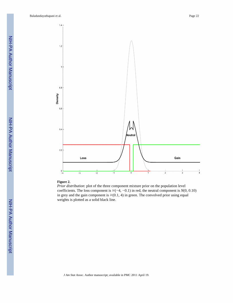
Figure 2.Prior distribution: plot of the three component mixture prior on the population levelcoefficients. The loss component is (−4, −0.1) in red, the neutral component is N(0, 0.10)in grey and the gain component is (0.1, 4) in green. The convolved prior using equalweights is plotted as a solid black line.
Baladandayuthapani et al. Page 22
J Am Stat Assoc. Author manuscript; available in PMC 2011 April 19.
NIH
-PA Author Manuscript
NIH
-PA Author Manuscript
NIH
-PA Author Manuscript
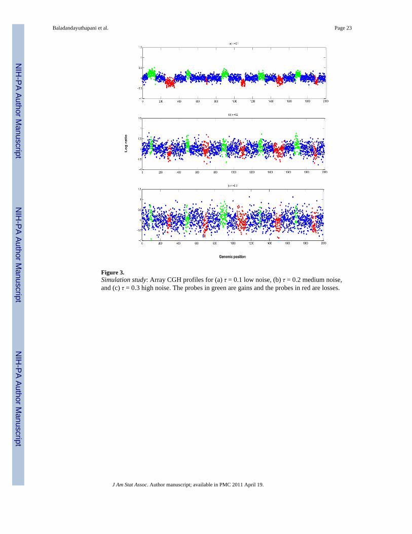
Figure 3.Simulation study: Array CGH profiles for (a) τ = 0.1 low noise, (b) τ = 0.2 medium noise,and (c) τ = 0.3 high noise. The probes in green are gains and the probes in red are losses.
Baladandayuthapani et al. Page 23
J Am Stat Assoc. Author manuscript; available in PMC 2011 April 19.
NIH
-PA Author Manuscript
NIH
-PA Author Manuscript
NIH
-PA Author Manuscript
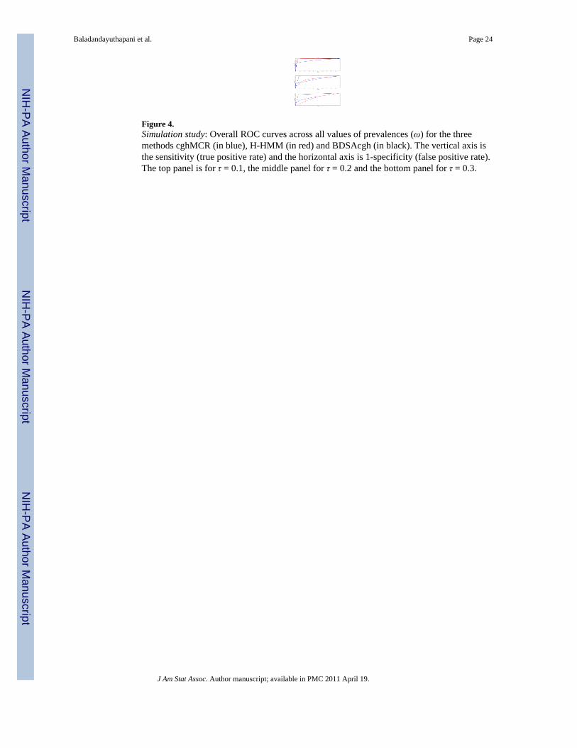
Figure 4.Simulation study: Overall ROC curves across all values of prevalences (ω) for the threemethods cghMCR (in blue), H-HMM (in red) and BDSAcgh (in black). The vertical axis isthe sensitivity (true positive rate) and the horizontal axis is 1-specificity (false positive rate).The top panel is for τ = 0.1, the middle panel for τ = 0.2 and the bottom panel for τ = 0.3.
Baladandayuthapani et al. Page 24
J Am Stat Assoc. Author manuscript; available in PMC 2011 April 19.
NIH
-PA Author Manuscript
NIH
-PA Author Manuscript
NIH
-PA Author Manuscript
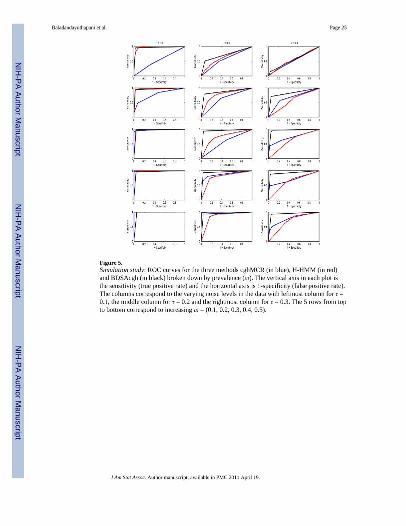
Figure 5.Simulation study: ROC curves for the three methods cghMCR (in blue), H-HMM (in red)and BDSAcgh (in black) broken down by prevalence (ω). The vertical axis in each plot isthe sensitivity (true positive rate) and the horizontal axis is 1-specificity (false positive rate).The columns correspond to the varying noise levels in the data with leftmost column for τ =0.1, the middle column for τ = 0.2 and the rightmost column for τ = 0.3. The 5 rows from topto bottom correspond to increasing ω = (0.1, 0.2, 0.3, 0.4, 0.5).
Baladandayuthapani et al. Page 25
J Am Stat Assoc. Author manuscript; available in PMC 2011 April 19.
NIH
-PA Author Manuscript
NIH
-PA Author Manuscript
NIH
-PA Author Manuscript

Figure 6.Simulation study: top panel are the bar graphs of the mean area under the curves (AUCs)with the standard error bars for the BDSAcgh (in red), cghMCR (in orange) and HHMM (inyellow). The vertical axes are the mean AUC with the horizontal axes sorted by increasingprevalence. The leftmost panel is for τ = 0.1 (low noise), middle panel is for τ = 0.2 (mediumnoise), and rightmost panel is for τ = 0.3 (high noise). Bottom panel: similar to top panelwith the vertical bar being the mean AUC20
Baladandayuthapani et al. Page 26
J Am Stat Assoc. Author manuscript; available in PMC 2011 April 19.
NIH
-PA Author Manuscript
NIH
-PA Author Manuscript
NIH
-PA Author Manuscript

Figure 7.Group profiles for chromosome 9: shown are the pointwise posterior probabilities of sharedregions of aberration as a function of the genomic position, p+(x) and p−(x), for the fourphenotypic groups: NA, NS, SC, and SV (top to bottom). The blue dotted lines indicate thethreshold for flagging a location as significant, controlling the expected Bayesian FDR to beless than 0.10. The locations that show a gain in copy number are shown in green, losses areshowin in red and neutral locations are shown in gray.
Baladandayuthapani et al. Page 27
J Am Stat Assoc. Author manuscript; available in PMC 2011 April 19.
NIH
-PA Author Manuscript
NIH
-PA Author Manuscript
NIH
-PA Author Manuscript
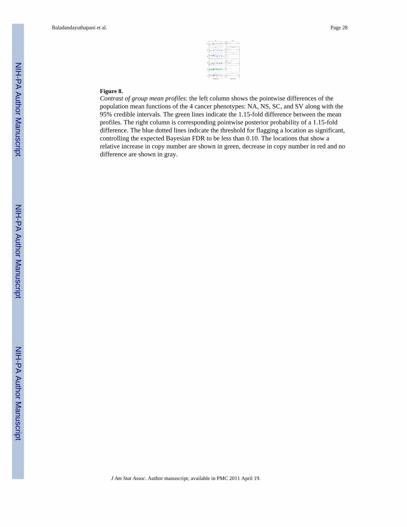
Figure 8.Contrast of group mean profiles: the left column shows the pointwise differences of thepopulation mean functions of the 4 cancer phenotypes: NA, NS, SC, and SV along with the95% credible intervals. The green lines indicate the 1.15-fold difference between the meanprofiles. The right column is corresponding pointwise posterior probability of a 1.15-folddifference. The blue dotted lines indicate the threshold for flagging a location as significant,controlling the expected Bayesian FDR to be less than 0.10. The locations that show arelative increase in copy number are shown in green, decrease in copy number in red and nodifference are shown in gray.
Baladandayuthapani et al. Page 28
J Am Stat Assoc. Author manuscript; available in PMC 2011 April 19.
NIH
-PA Author Manuscript
NIH
-PA Author Manuscript
NIH
-PA Author Manuscript
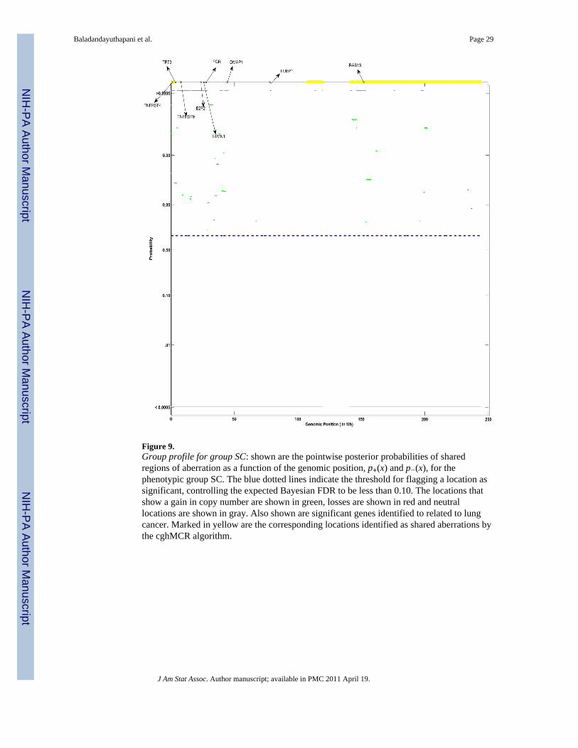
Figure 9.Group profile for group SC: shown are the pointwise posterior probabilities of sharedregions of aberration as a function of the genomic position, p+(x) and p−(x), for thephenotypic group SC. The blue dotted lines indicate the threshold for flagging a location assignificant, controlling the expected Bayesian FDR to be less than 0.10. The locations thatshow a gain in copy number are shown in green, losses are shown in red and neutrallocations are shown in gray. Also shown are significant genes identified to related to lungcancer. Marked in yellow are the corresponding locations identified as shared aberrations bythe cghMCR algorithm.
Baladandayuthapani et al. Page 29
J Am Stat Assoc. Author manuscript; available in PMC 2011 April 19.
NIH
-PA Author Manuscript
NIH
-PA Author Manuscript
NIH
-PA Author Manuscript

NIH
-PA Author Manuscript
NIH
-PA Author Manuscript
NIH
-PA Author Manuscript
Baladandayuthapani et al. Page 30
Table 1
Simulation Study: Shown here are the mean area under the curves (AUCs) for the three methods, cghMCR, H-HMM and BDSAcgh for various levels of noise (τ). The 3rd column shows the full AUCs and the 4th columnshows the partial area under the curves (AUC20) truncated at false positive rate of 0.2. Also shown are thestandard errors in parentheses.
τ Method AUC AUC20
0.10 cghMCR 0.8326 (0.0402) 0.7170 (0.0850)
H-HMM 0.9746 (0.0079) 0.8870 (0.0331)
BDSAcgh 0.9599 (0.0152) 0.8644 (0.0288)
0.20 cghMCR 0.7072 (0.0779) 0.5111 (0.0911)
H-HMM 0.7571 (0.0407) 0.3825 (0.0952)
BDSAcgh 0.9450 (0.0128) 0.7872 (0.0378)
0.30 cghMCR 0.6755 (0.0839) 0.4306 (0.0985)
H-HMM 0.6160 (0.0711) 0.1636 (0.0777)
BDSAcgh 0.9149 (0.0270) 0.7554 (0.0337)
J Am Stat Assoc. Author manuscript; available in PMC 2011 April 19.
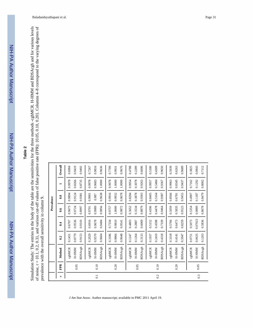
NIH
-PA Author Manuscript
NIH
-PA Author Manuscript
NIH
-PA Author Manuscript
Baladandayuthapani et al. Page 31
Tabl
e 2
Sim
ulat
ion
Stud
y: T
he e
ntrie
s in
the
body
of t
he ta
ble
are
the
sens
itivi
ties f
or th
e th
ree
met
hods
-cgh
MC
R. H
-HM
M a
nd B
DSA
cgh
and
for v
ario
us le
vels
of n
oise
, τ =
{0.
1, 0
.2, 0
.3},
and
var
ious
cut
-off
val
ues o
f fal
se p
ositi
ve ra
te (F
PR):
{0.0
5, 0
.10,
0.2
0}. C
olum
ns 4
–8 c
orre
spon
d to
the
vary
ing
degr
ees o
fpr
eval
ence
with
the
over
all s
ensi
tivity
in c
olum
n 9.
Prev
alen
ce
τFP
RM
etho
d0.
20.
40.
60.
81
Ove
rall
0.1
0.05
cghM
CR
0.14
510.
6707
0.96
730.
9894
0.99
780.
6984
H-H
MM
0.87
790.
9536
0.97
240.
9124
0.82
660.
9419
BD
SAcg
h0.
9153
0.93
100.
8997
0.93
810.
8735
0.94
92
0.10
cghM
CR
0.20
290.
6916
0.97
010.
9901
0.99
780.
7267
H-H
MM
0.95
700.
9678
0.99
890.
987
0.96
830.
9816
BD
SAcg
h0.
9604
0.94
840.
9856
0.96
381.
0000
0.96
36
0.20
cghM
CR
0.31
860.
7334
0.97
570.
9916
0.99
780.
7709
H-H
MM
0.98
660.
9810
1.00
000.
9932
1.00
000.
9931
BD
SAcg
h0.
9648
0.95
410.
9872
0.96
781.
0000
0.96
76
0.2
0.05
cghM
CR
0.12
470.
4803
0.36
520.
8284
0.99
540.
4788
H-H
MM
0.12
640.
2887
0.35
340.
3878
0.30
780.
2289
BD
SAcg
h0.
3133
0.60
690.
8879
0.93
030.
9263
0.66
96
0.10
cghM
CR
0.19
370.
5152
0.43
960.
8405
0.99
570.
5180
H-H
MM
0.24
100.
4598
0.44
780.
5164
0.54
840.
4309
BD
SAcg
h0.
4318
0.73
390.
9464
0.93
870.
9367
0.96
50
0.20
cghM
CR
0.33
180.
5766
0.50
590.
8566
0.99
630.
5939
H-H
MM
0.41
410.
6473
0.58
350.
6781
0.83
450.
6263
BD
SAcg
h0.
5947
0.82
590.
9523
0.94
550.
9437
0.96
89
0.3
0.05
cghM
CR
0.07
510.
5073
0.53
540.
4907
0.71
620.
3825
H-H
MM
0.06
350.
0702
30.
0889
0.11
870.
1292
0.08
43
BD
SAcg
h0.
1203
0.58
360.
8678
0.84
790.
8002
0.71
12
J Am Stat Assoc. Author manuscript; available in PMC 2011 April 19.
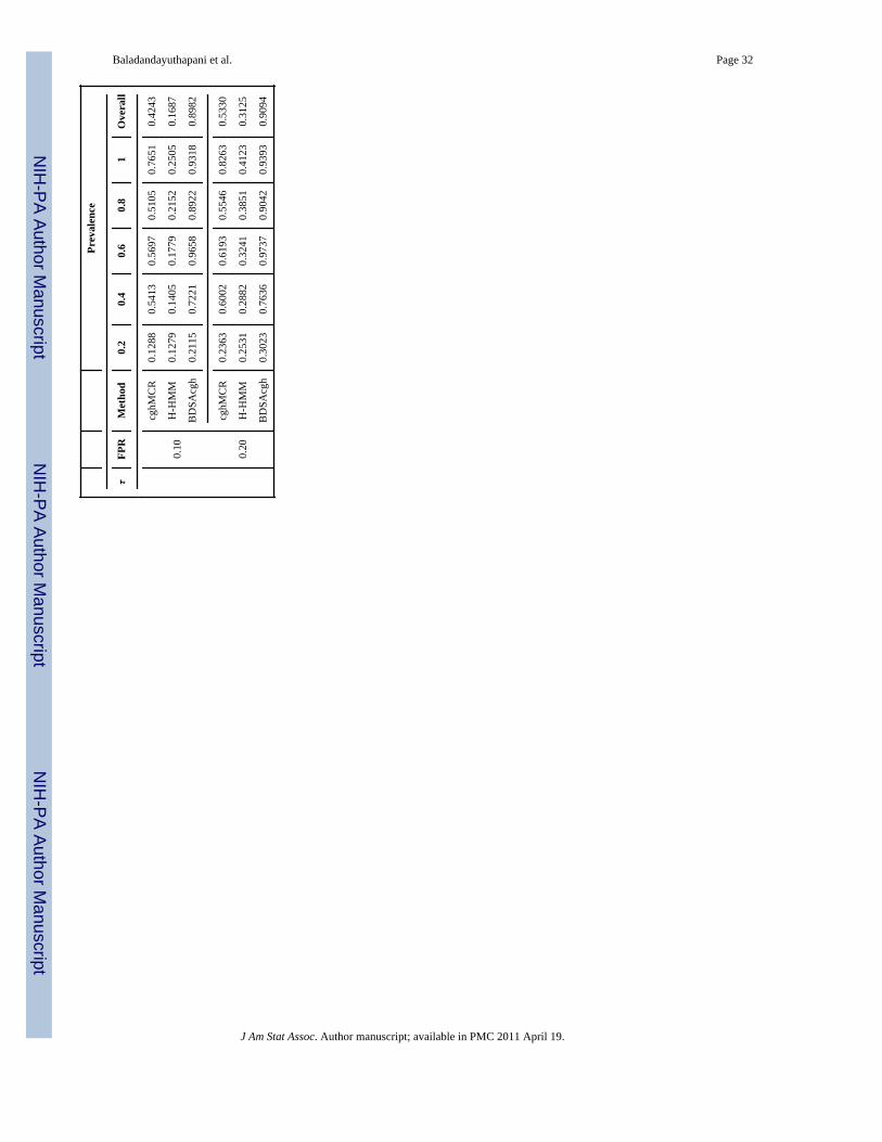
NIH
-PA Author Manuscript
NIH
-PA Author Manuscript
NIH
-PA Author Manuscript
Baladandayuthapani et al. Page 32
Prev
alen
ce
τFP
RM
etho
d0.
20.
40.
60.
81
Ove
rall
0.10
cghM
CR
0.12
880.
5413
0.56
970.
5105
0.76
510.
4243
H-H
MM
0.12
790.
1405
0.17
790.
2152
0.25
050.
1687
BD
SAcg
h0.
2115
0.72
210.
9658
0.89
220.
9318
0.89
82
0.20
cghM
CR
0.23
630.
6002
0.61
930.
5546
0.82
630.
5330
H-H
MM
0.25
310.
2882
0.32
410.
3851
0.41
230.
3125
BD
SAcg
h0.
3023
0.76
360.
9737
0.90
420.
9393
0.90
94
J Am Stat Assoc. Author manuscript; available in PMC 2011 April 19.
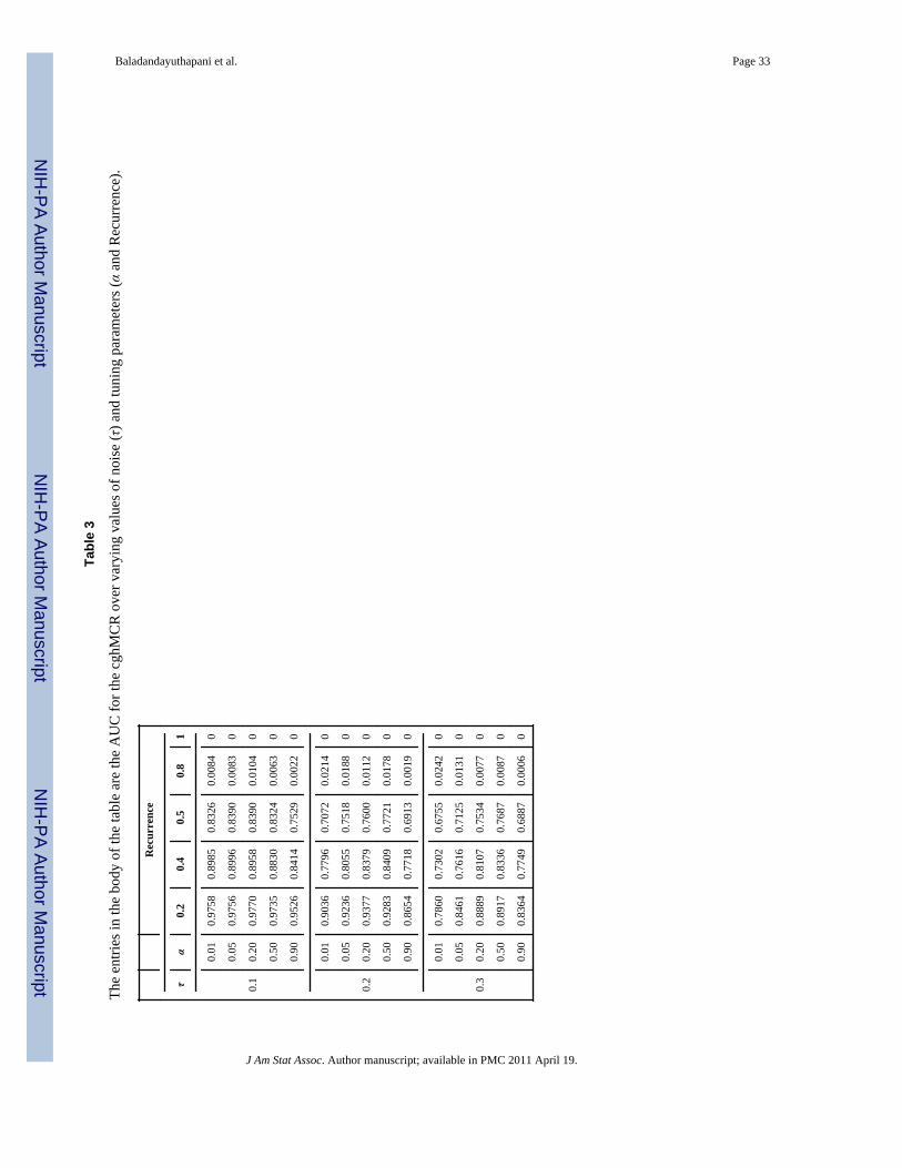
NIH
-PA Author Manuscript
NIH
-PA Author Manuscript
NIH
-PA Author Manuscript
Baladandayuthapani et al. Page 33
Tabl
e 3
The
entri
es in
the
body
of t
he ta
ble
are
the
AU
C fo
r the
cgh
MC
R o
ver v
aryi
ng v
alue
s of n
oise
(τ) a
nd tu
ning
par
amet
ers (α
and
Rec
urre
nce)
.
Rec
urre
nce
τα
0.2
0.4
0.5
0.8
1
0.1
0.01
0.97
580.
8985
0.83
260.
0084
0
0.05
0.97
560.
8996
0.83
900.
0083
0
0.20
0.97
700.
8958
0.83
900.
0104
0
0.50
0.97
350.
8830
0.83
240.
0063
0
0.90
0.95
260.
8414
0.75
290.
0022
0
0.2
0.01
0.90
360.
7796
0.70
720.
0214
0
0.05
0.92
360.
8055
0.75
180.
0188
0
0.20
0.93
770.
8379
0.76
000.
0112
0
0.50
0.92
830.
8409
0.77
210.
0178
0
0.90
0.86
540.
7718
0.69
130.
0019
0
0.3
0.01
0.78
600.
7302
0.67
550.
0242
0
0.05
0.84
610.
7616
0.71
250.
0131
0
0.20
0.88
890.
8107
0.75
340.
0077
0
0.50
0.89
170.
8336
0.76
870.
0087
0
0.90
0.83
640.
7749
0.68
870.
0006
0
J Am Stat Assoc. Author manuscript; available in PMC 2011 April 19.
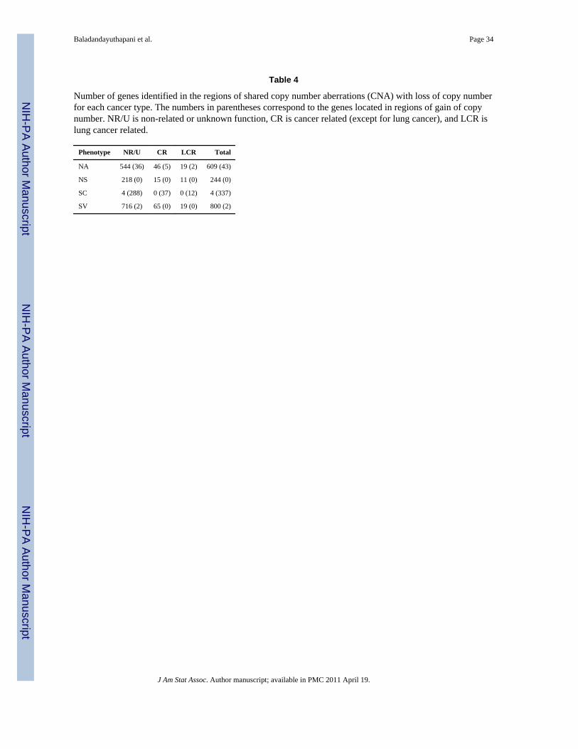
NIH
-PA Author Manuscript
NIH
-PA Author Manuscript
NIH
-PA Author Manuscript
Baladandayuthapani et al. Page 34
Table 4
Number of genes identified in the regions of shared copy number aberrations (CNA) with loss of copy numberfor each cancer type. The numbers in parentheses correspond to the genes located in regions of gain of copynumber. NR/U is non-related or unknown function, CR is cancer related (except for lung cancer), and LCR islung cancer related.
Phenotype NR/U CR LCR Total
NA 544 (36) 46 (5) 19 (2) 609 (43)
NS 218 (0) 15 (0) 11 (0) 244 (0)
SC 4 (288) 0 (37) 0 (12) 4 (337)
SV 716 (2) 65 (0) 19 (0) 800 (2)
J Am Stat Assoc. Author manuscript; available in PMC 2011 April 19.

NIH
-PA Author Manuscript
NIH
-PA Author Manuscript
NIH
-PA Author Manuscript
Baladandayuthapani et al. Page 35
Table 5
List of lung cancer related genes for each phenotypic group. All genes correspond to regions of loss of copynumber except the ones marked with an asterisk(*), which correspond to gain in copy number
NA NS SC SV
CD274 CDKN2A CD274* CD274
CDKN2A CDKN2B DAB2IP* CDKN2A
CDKN2B ELAVL2 DBC1* CDKN2B
DOCK8 IFNA17 FPGS* DOCK8
ELAVL2 IFNB1 JMJD2C* ELAVL2
FRMD3 IGFBPL1 PHF19* FRMD3
IFNA17 MTAP PRSS3* IFNA17
IFNB1 RECK PTENP1* IFNB1
IGFBPL1 RPS6 PTPRD* JMJD2C
JMJD2C SHB RAPGEF1* MIRNLET7A1
MTAP TUSC1 RPL12* MTAP
PTPRD TOPORS* NR4A3
RPS6 NTRK2
SHB PTPRD
TLE1 RPS6
TUSC1 SLC44A1
UBQLN1 TLE1
CA9* TUSC1
RAPGEF1* UBQLN1
J Am Stat Assoc. Author manuscript; available in PMC 2011 April 19.
Related Documents


