Nigeria’ Power Sector: Analysis of Productivity …cesa/files/WP_DE_CESA2011.… ·  · 2011-03-28A Comparative Analysis of Productivity Change in Italian and ... Efficiency analysis

Carlos Pestana Barros & Nicolas Peypoch

A Comparative Analysis of Productivity Change in Italian and Portuguese Airports

WP 006/2007/DE _________________________________________________________

Carlos Pestana Barros, Ade Ibiwoye and Shunsuke Managi

Nigeria’ Power Sector: Analysis of Productivity

WP 10/2011/DE/UECE

_________________________________________________________

Department of Economics

WORKING PAPERS

ISSN Nº 0874-4548

School of Economics and Management TECHNICAL UNIVERSITY OF LISBON

1

Nigeria’ Power Sector: Analysis of Productivity

Carlos Pestana Barros1, Ade Ibiwoye2, and Shunsuke Managi3,4

1. Corresponding author: Instituto Superior de Economia e Gestão; Technical University of Lisbon Rua Miguel Lupi, 20; 1249-078 - Lisbon, Portugal and UECE (Research Unit on Complexity and Economics) and CESA (Center for African and Development Studies). Phone: +351 - 213 016115; fax: +351 - 213 925 912. Email: [email protected]

(Corresponding author). 2Department of Actuarial Science, University of Lagos, Nigeria. Email: [email protected]

3 Institute for Global Environmental Strategies, Japan; [email protected]

Abstract: This study analyzes the productivity change in Nigeria’s power sector from 2004-2008,

Applying the Malmquist index with the input technological bias. The results show that on average, the

Nigerian power sector becomes both more efficient and experience technological improvements.

Furthermore, the assumption of Hicks neutral technological change is not suitable and therefore

the traditional growth accounting method is not appropriate for analyzing changes in

productivity for Nigeria power sector. Policy implications are derived.

Key words: Power, Nigeria; productivity, technological change, policy implications.

2

1. Introduction

Nigeria needs to improve efficiency and reduce waste in the public sector, and strengthen

the private sector as its engine of growth (Ebohon, 1996; Akinlo, 2008; Wolde-Rufael, 2009). It

is generally accepted that this feature will only be achievable with an efficient electricity

generation as the latter affects every gamut of the economy. Unfortunately, although the power

sector is one of the most important industries supporting infrastructure of the country electricity

generation had remained underdeveloped and in short supply. While the country is richly

endowed with huge supply of gas, coal, as well as solar and hydro resources, these seemed to be

only sparingly applied. Currently, power generation is mainly from thermal plants, which

contribute about 60%, and hydro power plants which generate about 30%( Tallapragada, 2009;

Adoghe, 2008; Okoro and Chikuni, 2007).

The motivation for the present research are the following. First, the context of the Nigerian

electricity market, characterised by inadequate electricity generation framework, which is

continues to be compounded by lack of timely routine maintenance, thereby resulting in

significant deterioration in plant electricity output, a key reason for the lingering electric power

crisis. More than two decades of underprivileged planning and underinvestment had left a vast

supply deficit (Ikeme and Ebohon, 2005). Also, none of the new infrastructure in over a decade,

unfortunately, comes in the market of the country despite rapid population growth and rising

demand for power. The power sector was at the edge of fall down. Average daily generation was

1,750MW in 1999. The situation, after 10 years, is not really different as available capacity

output is still less than 2.5GW. Various measures taken in the past to address the electricity

generation and distribution problem seemed to have yielded little or no result. This apparently

3

led government, in 2004, to embark on a reform that was meant to decentralize operations in the

power sector. Conceptually, the reforms are to solve a myriad of problems, including limited

access to infrastructure, low connection rates, inadequate power generation capacity, inefficient

usage of capacity, and lack of capital for investment, ineffective regulation, high technical losses

and vandalism, and insufficient transmission and distribution facilities (Adenikinju, 2003). In

short, Nigeria seeks policies that can promote least-cost electricity generation while ensuring a

constant increase in production. Second, to adopt a performance model aiming to analyse the

production of Nigerian electricity plants to investigate whether there are improvements in

efficiency and productivity in the sector after the reform. Therefore this study applies a data

envelopment analysis (DEA) model to the Malmquist Index with biased technological change to

frame the productivity change of Nigeria’s power stations, Farrell (1957). Finally, this research

aims to identify a sound energy policy that can assist Nigeria to improve its energy capacity

through improved performance.

The remainder of the paper is organized as follows: Section 2 presents the contextual

setting; Section 3 presents a literature survey. Section 4 details the methodology while Section 5

presents the data and the results. Section 6 discusses the results and section 7 concludes.

2. Contextual setting

Electricity generation in Nigeria started in the city of Lagos in 1896 some 15 years after that of

Britain from which Nigeria obtained independence in 1960. In the northern part of the country,

the Nigeria Electricity Supply Company (NESCO) began operations in 1929 as an electric utility

company in Nigeria with the construction of a hydroelectric power station at Kurra near Jos. The

first attempt to coordinate supply and development of electricity occurred in 1951 with the

4

establishment of the Electricity Corporation of Nigeria (ECN) by an act of parliament. In 1962,

the first 132KV line was constructed, connecting Ijora Power Station to Ibadan Power Station.

The Niger Dams Authority (NDA) was established in 1962 and authorized to build up the

hydropower prospects of the country. It sold electricity to ECN. However, ECN and NDA were

merged in 1972 to form the National Electric Power Authority (NEPA), a company with

exclusive monopoly over electricity generation, transmission, distribution and sales throughout

the country.

Despite its long history, NEPA’s development has been very slow and electricity

generation in Nigeria had deteriorated over the years. This is rarely expected given the country’s

rich endowment in natural resources that could facilitate electricity production. The company

from inception appeared to be faced with the problems of lack of adequate funding and

managerial strategies resulting in the steady decline of the company (Adoghe, 2008). While the

transmission and distribution deteriorated, the demand for electricity continued to increase. This

is in spite of the fact that many corporate organisations have folded up as a result of harsh

operating environment occasioned, in large part, by the poor and epileptic supply of electricity.

The paradox is easily explained by the increasing demand in domestic requirement resulting

from an ever-increasing population. Analysts (see Tallapragada, 2009; Adoghe, 2008; Okoro

and Chikuni, 2007) have advanced some reasons for the continued problem in the sector. A huge

investment was undertaken in the area of power generation without a corresponding investment

in the transmission and distribution networks. Other reasons identified include weak

governance, poor institutional capacities and inadequate investments. It is a classic example of

the developmental paradox where there are tremendous resources but little dividends.

Nigeria’s economy is characterized by a large informal sector many of whom depend on

electricity for daily production and livelihood. As NEPA is almost never available many of them

5

have been forced to buy generators to continue production. This immediately has the effect of

increasing their cost of production. Those who cannot afford the luxury are forced to abandon

the trade often for no visible alternative. The result is that the rate of unemployment continues to

rise and rise. The experience in the formal sector is not much different, as corporate bodies have

had to self-generate electricity in order to maintain production.

There is a lot of suspicion and conflicts between NEPA officials as provider on the one

hand and consumers on the other thereby encouraging illegitimate activities such as illegal

connections to the national grid or the existing residential/industrial outfit, overbilling and under

billing, payment via unscrupulous business collusion, and canalization of equipments which are

then resold, in most cases, to private electricity institutions (Subair and Oke, 2008).

Often NEPA is confronted with reckless development of areas, which does not match its

efforts. For example, small industries unexpectedly spring up in areas planned as residential. As

a consequence, transformers and cables are overloaded until they are damaged. This is

problematic since NEPA is not notified when new loads are added to existing ones.

The costs of power supply interruptions are fairly large because of the predominating

utilization of private generators for homes and industries with its fire and health hazards,

disturbance of scheduled productive activities and reductions in operation. Not only that, the

unpredictable power supply often results in equipments malfunctioning (Subair and Oke,

2008).Currently, the National electricity grid presently consists of nine generating stations (3

hydro and 6 thermal). However, as stated, supply capacity largely lags behind demand of the

country. Although some state capitals are connected to the national transmission grid system

they are served only haphazardly. In the circumstance, the proposed national integrated rural

development is elusive as disabilities are experienced in every facet of NEPA operations.

6

In 2000 government restructured the power sector by unbundling NEPA into eighteen

separate companies composed of six electricity-generating companies, one Transmission

Company and eleven distribution companies. The restructuring was designed to encourage

private participation by breaking NEPA’s monopoly and paving way for Independent Power

Producers (IPPs). It is yet to be seen whether the reform will bring about the much desired

changes as the new structure is yet to be fully operational.

3. Literature Survey

While there is extensive literature on benchmarking applied to a diverse range of economic

fields, the scarcity of studies regarding African energy companies’ bear’s testimony to the fact

that this is a relatively under-researched topic (Estache, Tovar and Trujillo, 2008).

Efficiency analysis in relation to electricity is concentrated on distribution networks (Jamasb,

Nillesen and Pollitt, 2004; Farsi and Filippini, 2004; Estache, Rossi and Ruzzier, 2004; Jamasb

and Pollitt, 2003). Papers analysing the efficiency of electricity generating plants include (Kleit

and Terrell, 2001; Hiebert, 2002; Arocena and Wadams Price, 2002; Knittel, 2002; Raczka,

2001; Barros, 2008). Jamasb and Pollitt (2001) review the frequency with which different input

and output variables are used to model electricity distribution. The most frequently used outputs

are units of energy delivered, number of customers and size of the service area. The most widely

used inputs are number of employees, transformer capacity and network length. For an extended

up to date survey, see Jamasb, Mota, Newbery and Pollitt (2005).

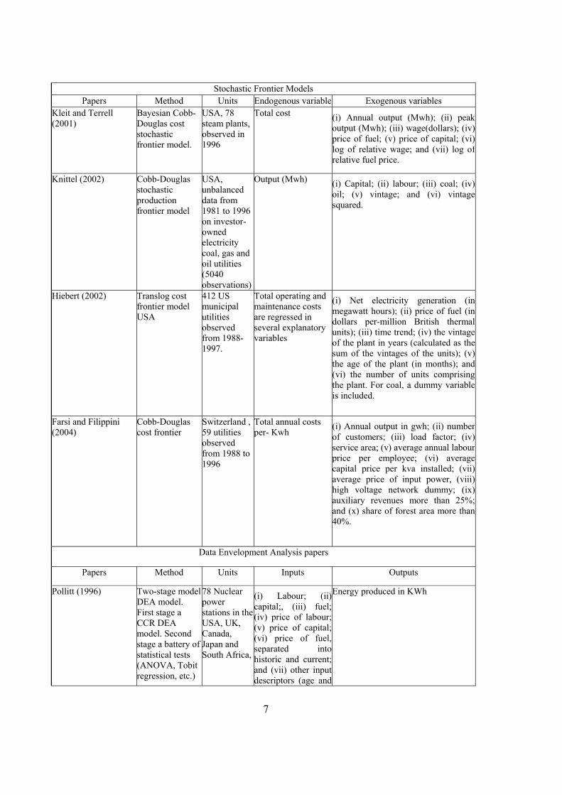
Restricting the literature review to a sample of recent energy production papers, it is observed

that they adopt one of two complementary efficiency methodologies: DEA, and the Stochastic

Frontier Model. Table 1 displays our review of these works.

Table 1: Recent Papers on Energy Production

7

Stochastic Frontier Models Papers Method Units Endogenous variable Exogenous variables

Kleit and Terrell (2001)

Bayesian Cobb-Douglas cost stochastic frontier model.

USA, 78 steam plants, observed in 1996

Total cost (i) Annual output (Mwh); (ii) peak output (Mwh); (iii) wage(dollars); (iv) price of fuel; (v) price of capital; (vi) log of relative wage; and (vii) log of relative fuel price.

Knittel (2002) Cobb-Douglas stochastic production frontier model

USA, unbalanced data from 1981 to 1996 on investor-owned electricity coal, gas and oil utilities (5040 observations)

Output (Mwh) (i) Capital; (ii) labour; (iii) coal; (iv) oil; (v) vintage; and (vi) vintage squared.

Hiebert (2002) Translog cost frontier model USA

412 US municipal utilities observed from 1988-1997.

Total operating and maintenance costs are regressed in several explanatory variables

(i) Net electricity generation (in megawatt hours); (ii) price of fuel (in dollars per-million British thermal units); (iii) time trend; (iv) the vintage of the plant in years (calculated as the sum of the vintages of the units); (v) the age of the plant (in months); and (vi) the number of units comprising the plant. For coal, a dummy variable is included.

Farsi and Filippini (2004)

Cobb-Douglas cost frontier

Switzerland , 59 utilities observed from 1988 to 1996

Total annual costs per- Kwh (i) Annual output in gwh; (ii) number

of customers; (iii) load factor; (iv) service area; (v) average annual labour price per employee; (vi) average capital price per kva installed; (vii) average price of input power, (viii) high voltage network dummy; (ix) auxiliary revenues more than 25%; and (x) share of forest area more than 40%.

Data Envelopment Analysis papers

Papers Method Units Inputs Outputs

Pollitt (1996) Two-stage model DEA model. First stage a CCR DEA model. Second stage a battery of statistical tests (ANOVA, Tobit regression, etc.)

78 Nuclear power stations in the USA, UK, Canada, Japan and South Africa,

(i) Labour; (ii) capital;, (iii) fuel; (iv) price of labour; (v) price of capital; (vi) price of fuel, separated into historic and current; and (vii) other input descriptors (age and

Energy produced in KWh

8

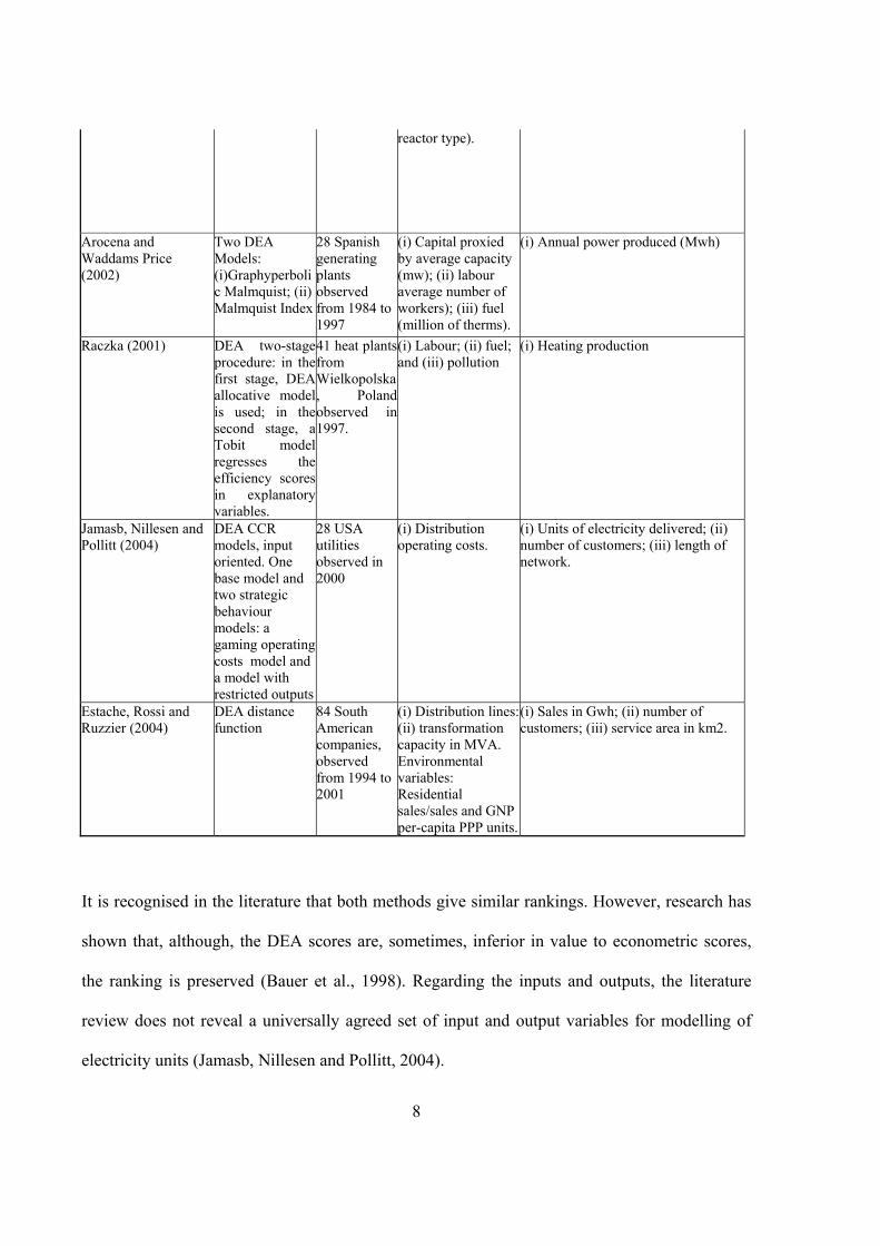
reactor type).

Arocena and Waddams Price (2002)

Two DEA Models: (i)Graphyperbolic Malmquist; (ii) Malmquist Index

28 Spanish generating plants observed from 1984 to 1997

(i) Capital proxied by average capacity (mw); (ii) labour average number of workers); (iii) fuel (million of therms).

(i) Annual power produced (Mwh)

Raczka (2001) DEA two-stage procedure: in thefirst stage, DEAallocative modelis used; in thesecond stage, aTobit modelregresses theefficiency scoresin explanatoryvariables.

41 heat plantsfrom Wielkopolska, Polandobserved in1997.

(i) Labour; (ii) fuel; and (iii) pollution

(i) Heating production

Jamasb, Nillesen and Pollitt (2004)

DEA CCR models, input oriented. One base model and two strategic behaviour models: a gaming operating costs model and a model with restricted outputs

28 USA utilities observed in 2000

(i) Distribution operating costs.

(i) Units of electricity delivered; (ii) number of customers; (iii) length of network.

Estache, Rossi and Ruzzier (2004)

DEA distance function

84 South American companies, observed from 1994 to 2001

(i) Distribution lines: (ii) transformation capacity in MVA. Environmental variables: Residential sales/sales and GNP per-capita PPP units.

(i) Sales in Gwh; (ii) number of customers; (iii) service area in km2.

It is recognised in the literature that both methods give similar rankings. However, research has

shown that, although, the DEA scores are, sometimes, inferior in value to econometric scores,

the ranking is preserved (Bauer et al., 1998). Regarding the inputs and outputs, the literature

review does not reveal a universally agreed set of input and output variables for modelling of

electricity units (Jamasb, Nillesen and Pollitt, 2004).

9

The policy implications of the surveyed papers focus on the differences in efficiency scores and

the drivers of efficiency, the role of alternative regulatory frameworks in efficiency, and the

comparative analysis of efficiency of public and private companies. Other findings are:

Deregulating electricity generation increases efficiency (Kleit and Terrell, 2000), alternative

regulatory programs provide firms with an incentive to increase efficiency (Knittel, 2002),

andprice controls and subsidies decrease technical efficiency (Raczka, 2001). Moreover,

regulation and competition accompanied by privatisation promotes efficiency (Arocena and

Waddams Price, 2002), while regulation without competition decrease efficiency (Barros and

Peypoch, 2008). For competition to work, regulators must coordinate their policy throughout a

multi country region, for example, South America, (Estache, Rossi and Ruzzier, 2004), Africa

(Ramanathan, 2005; Estache, Tovar and Trujillo,2008, Barros and Managi 2009)

Privately-owned plants exhibit higher average efficiency than publicly-owned plants (Pollitt,

1996). Public firms are more efficient under cost-of-service regulation, compared with price-cap

regulation (Arocena and Waddams Price, 2002). Another paper relying on an innovative cost

function is Jara Diaz et al. (2004). Recent applications of DEA models in energy studies are

Pombo and Taborda (2006) and Vaninski (2006), Nakano and Managi (2008) and Mukherjee

(2002). Therefore, the present paper innovates in energy efficiency adopting the Malmquist

DEA model with the input technological bias.

Research on Nigeria energy includes Ibitoye and Adenikinju (2007), Amobi (2007), Eti, Ogaji

and Probert (2004), Ikeme and Ebohon (2005) and Adenikinju (2003), but none of this papers

analysed productivity on Nigerian electricity plants.

10

4. The Model

We apply DEA to station-level data in order to measure changes in productivity in Nigeria’s

electricity industry for the period from 2004 to 2008. We separate measures of productivity

change into various component parts to better understand the effect of technological

advancement. Total factor productivity (TFP) includes all categories of productivity change,

which can be decomposed into two components: 1) technological change (i.e., shifts in the

production frontier) and 2) efficiency change (i.e., movement of inefficient production units

relative to the frontier) Färe et al. (1994)

Production frontier analysis provides the Malmquist indexes (Malmquist, 1953; Caves;

Christensen and Diewert, 1982), which can be used to quantify productivity change and can be

decomposed into various constituents. Malmquist Total Factor Productivity is a specific output-

based measure of TFP. It measures the TFP change between two data points by calculating the

ratio of two associated distance functions (Caves; Christensen and Diewert, 1982) . A key

advantage of the distance function approach is that it provides a convenient way to describe a

multi-input, multi-output production technology without the need to specify functional forms or

behavioural objectives, such as cost-minimization or profit-maximization.

The DEA method has been widely used to estimate the reciprocal of the Shephard (1970)

input distance function. The reciprocal of this distance function serves as a measure of Farrell

(1957) input efficiency and equals the proportional contraction in all inputs that can be feasibly

accomplished given output, if the decision making unit (DMU) adopts best-practice methods.

We link input efficiency indices across time in order to estimate the Malmquist productivity

index. This index estimates the change in resource use over time that is attributable to efficiency

change and technological change. Furthermore, we use the approach of Färe et all. (1997) and

11

decompose technological change into an index of output-biased technological change, an index

of input-biased technological change, and an index of the magnitude of technological change.

Holding outputs constant, the reciprocal of the input distance function gives the ratio of

minimum inputs required to produce a given level of outputs to actual inputs employed, and

serves as a measure of technical efficiency. Let 1( ,..., )t t tNx x x= represent a vector of N non-

negative inputs in period t and let 1( ,..., )t t tMy y y= represent a vector of M non-negative outputs

produced in period t. The input requirement set in period t represents the feasible input

combinations that can produce outputs and is represented as

( ) { : can produce }tF y x x y= . (1)

The isoquant for the input requirement set is defined as

( ) { : ( ), for 1}t txISOQ F y x F y λ

λ= ∉ > . (2)

The Shephard input distance function is defined as

( , ) max{ : ( )}t ti

xD y x F yλλ

= ∈ . (3)

The reciprocal of the Shephard input distance function equals the ratio of minimum

inputs to actual inputs employed and serves as a measure of Farrell input technical efficiency.

Efficient DMUs use inputs that are part of the ( )tISOQ F y and have ( , ) 1tiD y x = . Inefficient

DMUs have ( , ) 1tiD y x > .

We assume that there are k=1,…,K DMUs. The DEA piece-wise linear constant returns

to scale input requirement set takes the form:

1 1

( ) { : , 1,..., , , 1,..., , 0, 1,..., }.K K

t t t t t tk kn n k km m k

k kF y x z x x n N z y y m M z k K

= =

= ≤ = ≥ = ≥ =∑ ∑ (4)

12

The DEA input requirement set takes linear combinations of the observed inputs and

outputs of the K DMUs using the K intensity variables, tkz , to construct a best-practice

technology. The N+M inequality constraints associated with inputs and outputs imply that no

less input can be used to produce no more output than a linear combination of observed inputs

and outputs of the K DMUs. Constraining the K intensity variables to be non-negative allows

for constant returns to scale.

To compute input technical efficiency for DMU "o" we solve the following linear

programming problem:

1 1

, 1

1

1/ ( , ) max{ : , 1,..., ,

, 1,..., , 0, 1,..., }.

Kt t t t t ti o o k kn onz k

Kt t t tk km om k

k

D y x z x x n N

z y y m M z k K

λλ λ− −

=

=

= ≤ =

≥ = ≥ =

∑

∑ (5)

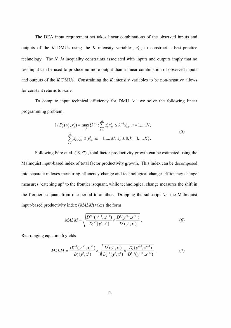
Following Färe et al. (1997) , total factor productivity growth can be estimated using the

Malmquist input-based index of total factor productivity growth. This index can be decomposed

into separate indexes measuring efficiency change and technological change. Efficiency change

measures "catching up" to the frontier isoquant, while technological change measures the shift in

the frontier isoquant from one period to another. Dropping the subscript "o" the Malmquist

input-based productivity index (MALM) takes the form

1 1 1 1 1

1

( , ) ( , )( , ) ( , )

t t t t t ti i

t t t t t ti i

D y x D y xMALMD y x D y x

+ + + + +

+= × . (6)

Rearranging equation 6 yields

1 1 1 1 1

1 1 1 1

( , ) ( , ) ( , )( , ) ( , ) ( , )

t t t t t t t t ti i i

t t t t t t t t ti i i

D y x D y x D y xMALMD y x D y x D y x

+ + + + +

+ + + += × × , (7)

13

Where efficiency change (i.e., movements towards the production frontier) is represented by

1 1 1( , )( , )

t t ti

t t ti

D y xEFFCHD y x

+ + +

= and technological progress is represented by

1 1

1 1 1 1

( , ) ( , )( , ) ( , )

t t t t t ti i

t t t t t ti i

D y x D y xTECHD y x D y x

+ +

+ + + += × . The TECH, EFFCH and other indexes are components

of Malmquist TFP index. Values of MALM, EFFCH, or TECH greater than one indicate

productivity growth in efficiency, and technological progress.

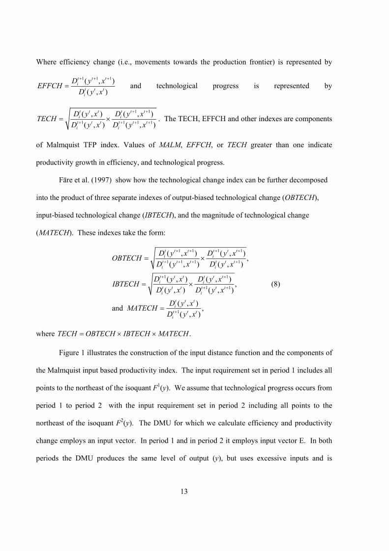
Färe et al. (1997) show how the technological change index can be further decomposed

into the product of three separate indexes of output-biased technological change (OBTECH),

input-biased technological change (IBTECH), and the magnitude of technological change

(MATECH). These indexes take the form:

1 1 1 1

1 1 1 1

1 1

1 1

1

( , ) ( , ) ,( , ) ( , )

( , ) ( , ) , ( , ) ( , )

( , )and , ( , )

t t t t t ti i

t t t t t ti i

t t t t t ti i

t t t t t ti i

t t ti

t t ti

D y x D y xOBTECHD y x D y x

D y x D y xIBTECHD y x D y x

D y xMATECHD y x

+ + + +

+ + + +

+ +

+ +

+

= ×

= ×

=

(8)

where .TECH OBTECH IBTECH MATECH= × ×

Figure 1 illustrates the construction of the input distance function and the components of

the Malmquist input based productivity index. The input requirement set in period 1 includes all

points to the northeast of the isoquant F1(y). We assume that technological progress occurs from

period 1 to period 2 with the input requirement set in period 2 including all points to the

northeast of the isoquant F2(y). The DMU for which we calculate efficiency and productivity

change employs an input vector. In period 1 and in period 2 it employs input vector E. In both

periods the DMU produces the same level of output (y), but uses excessive inputs and is

14

technically inefficient. The input distance function in period 1 is 1 1 0( , )0i

AD y xB

= and in period 2

the input distance function is 2 2( , ) 0 / 0 .iD y x E D= The two inter-period input distance functions

are calculated as 1 2 0( , )0i

ED y xF

= and 2 1 0( , )0i

AD y xC

= . The Malmquist index is calculated as

0 / 0 0 / 00 / 0 0 / 0E D E FMALMA C A B

= ×

. Efficiency change is calculated as 0 / 00 / 0E DEFFCHA B

= and

technological change is calculated as 0 / 0 0 / 0 0 00 / 0 0 / 0 0 0

A B E F C DTECHA C E D B F

= × = ×

.

<Figure 1 about here>

Figure 2 illustrates the construction of the index of input-biased technological change.

The isoquant in period 1 is represented by F1(y). We again assume technological progress and

draw two alternative isoquants represented by F21(y) and F22(y). Technological progress is

Hicks' neutral if the MRS (marginal rate of substitution) between two inputs remains constant,

holding the input mix constant. Hicks' neutral technological change is given by the parallel shift

in the input requirement set to FHN(y). Technological progress is x1-saving and x2-using if the

MRS between the two inputs increases, holding the input mix constant. Technological progress

is x1-using and x2-saving if the MRS between the two inputs decreases, holding the input mix

constant. The isoquant F21(y) represents an x1-saving and x2-using bias. The isoquant F22(y)

represent an x1-using and x2-saving bias. From period 1 to period 2 the ratio of the two inputs

changed such that1

1 1

2 2

t tx xx x

+

>

. If technological progress shifts the isoquant to F21(y) in

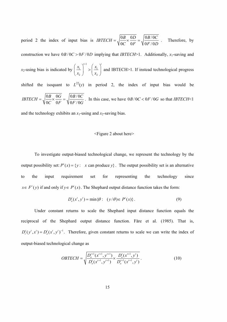
15

period 2 the index of input bias is 0 0 0 / 00 0 0 / 0

B D B CIBTECHC F F D

= × = . Therefore, by

construction we have 0 / 0 0 / 0B C F D> implying that IBTECH>1. Additionally, x1-saving and

x2-using bias is indicated by 1

1 1

2 2

t tx xx x

+

>

and IBTECH>1. If instead technological progress

shifted the isoquant to L22(y) in period 2, the index of input bias would be

0 0 0 / 00 0 0 / 0

B G B CIBTECHC F F G

= × = . In this case, we have 0 / 0 0 / 0B C F G< so that IBTECH<1

and the technology exhibits an x1-using and x2-saving bias.

<Figure 2 about here>

To investigate output-biased technological change, we represent the technology by the

output possibility set: ( ) { : can produce }tP x y x y= . The output possibility set is an alternative

to the input requirement set for representing the technology since

( ) if and only if ( )t tx F y y P x∈ ∈ . The Shephard output distance function takes the form:

( , ) min{ : ( / ) ( )}t t t toD x y y P xθ θ= ∈ . (9)

Under constant returns to scale the Shephard input distance function equals the

reciprocal of the Shephard output distance function. Färe et al. (1985). That is,

1( , ) ( , )t t t t t ti oD y x D x y −= . Therefore, given constant returns to scale we can write the index of

output-biased technological change as

1 1 1 1

1 1 1 1

( , ) ( , )( , ) ( , )

t t t t t to o

t t t t t to o

D x y D x yOBTECHD x y D x y

+ + + +

+ + + += × . (10)

16

Figure 3 illustrates the construction of the index of output-biased technological change

assuming technological progress between period 1 and 2. The output possibility set in period 1

is given by P1(x). Technological progress with respect to outputs is Hicks' neutral if the

marginal rate of transformation between two outputs is constant, holding the mix of outputs

constant. Hicks' neutral technological progress is illustrated by the parallel shift of the

production possibility set to PHN(x). Technological progress is biased in favour of output 1 (y1-

producing) if the marginal rate of transformation between outputs 1 and 2 increases, holding the

mix of outputs constant. Technological progress is biased in favour of output 2 (y2-producing),

if the marginal rate of transformation between the two outputs is less in period 2 holding the

output mix constant. The output possibility set given by P21(x) illustrates an y1-producing output

bias and the output possibility set given by P22(x) illustrates an y2-producing output bias.

In period 1 a DMU is observed to produce an output vector represented by point A. The

output distance function is calculated as 1 1 0( , )0o

AD x yB

= . In period 2, the DMU is observed to

produce output vector E. If the technology shifts to P21(x) in period 2, the output distance

function in period 2 is 2 2 0( , )0o

ED x yF

= and the index of output-biased technological change

is 0 / 0 0 / 0 0 / 0 10 / 0 0 / 0 0 / 0

E F A B D FOBTECHE D A C B C

= × = > . Thus, since 1

1 11

2 2

t t

t t

y yy y

+

+ < and OBTECH>1, the

technology is y1-producing, relative to y2. If the technology shifted to P22(x) in period 2, the

output distance function would be calculated as 2 2 0( , )0o

ED x yG

= and output-biased technological

change is 0 / 0 0 / 0 0 / 0 10 / 0 0 / 0 0 / 0

E G A B D GOBTECHE D A C B C

= × = < . Given that 1

1 11

2 2

t t

t t

y yy y

+

+ < and

OBTECH<1, the technology is y2-producing.

17

<Figure 3 about here>

In the next section we calculate input technical efficiency and the components of the

Malmquist input-based productivity index for Nigeria’s energy plants and examine the bias in

the use of inputs and production of outputs found in the technological change index.

5. Data and Results

5.1. Data

We compiled our dataset on nine Nigerian electricity plants from 2004 -2008 from several

sources (Federal Ministry of Power and Steel, 2006; NEPA Annual Accounts 2001 – 2008,

Okoro and Chikuni, 2007). In addition, private information was obtained from professionals in

the industry in Nigeria. These stations are Kainji Hydro Power, Jebba Hydro Power, Shiroro

Hydro Power, Afam Thermal Power, Delta Thermal Power, Egbin Thermal Power, Sapele

Thermal Power, Ijora Thermal Power, and Oji Thermal Power. Output is defined as gross

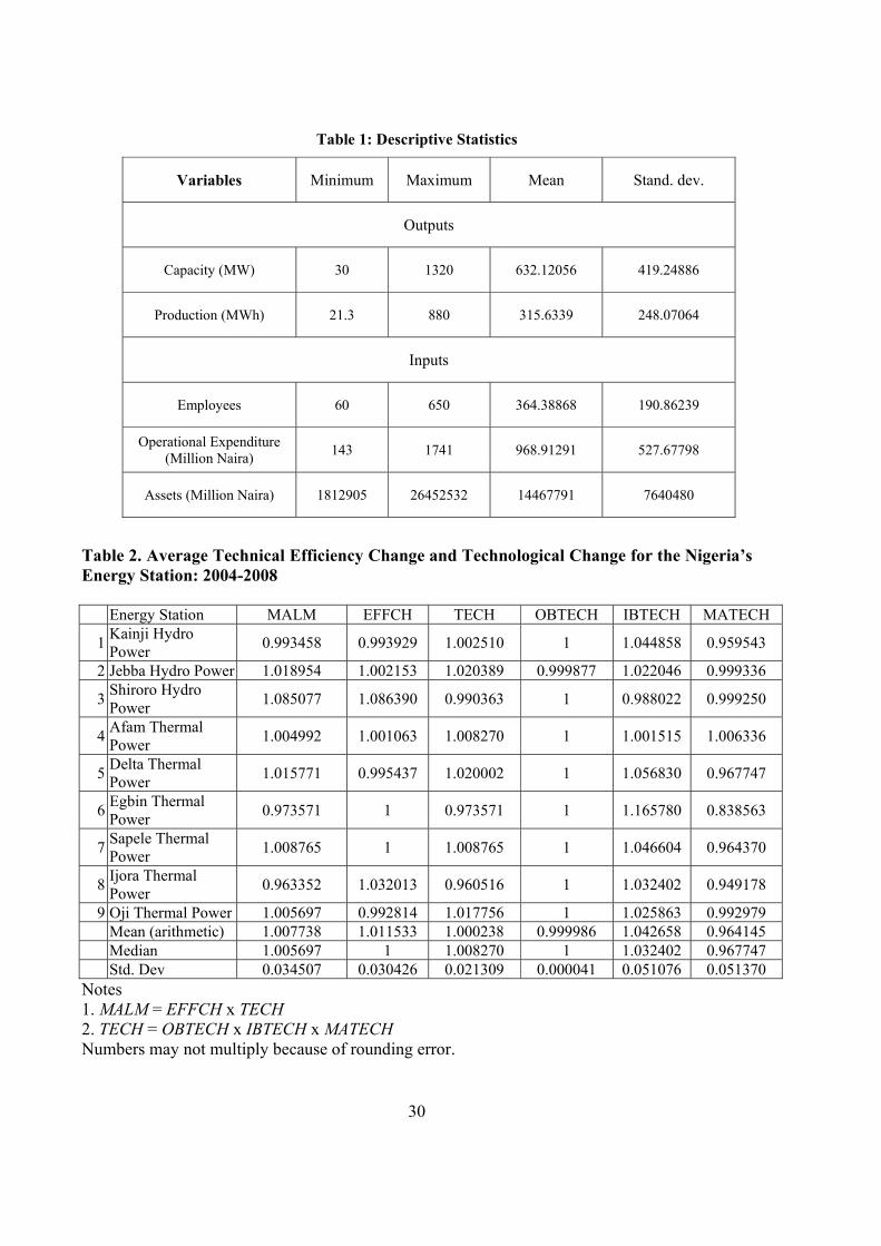
(MWh) and capacity (MW), Maloney et al. (1996). Inputs are employees (person), operational

expenditure (million Naira), and assets (million Naira). This study measures and decomposes

productivity change over time in Nigeria power sector. Then, the geometric mean of each

station-level index is provided to show the annual average of the indices.

<Table 2 about here>

5.2 Total Factor Productivity

Table 2 and Table 3 present the results for annual average change in TFP, and changes in

the TFP decomposed into the technological change and efficiency change. The rate of TFP is

larger than 1.0077. The rate of the TFP, however, drops from 1.092 and 1.023 in 2004-2005 and

18

2005-2006, respectively, to 0.978 and 0.937 in 2006-2007 and 2007-2008, respectively. A

similar trend appeared in TECH change with an average of 1.0178.

<Table 2 and 3 about here>

In contrast, the changes in EFFCH are always opposite direction indicating the TECH

dominates EFFCH on average. The magnitude of the change in EFFCH, however, is increasing

over study periods on average. That is, inefficient stations are catching up to the frontier. In

summary, we find TECH is the main source of TFP growth in Nigeria though there are catching

up effects (i.e., efficiency improvement) on average.

As a consequence of innovation, technological change occurs, That is, the adoption of

new technologies by best-practice power plant. The technological change index is greater than

one for all except three plants, which indicates technological improvement (TECH>1), while

others experienced technological regress (TECH<1).

We note that the power plants that defined the frontier in from 2004 and 2008

experienced positive change in efficiency. The EFFCH=1 only for Egbin Thermal Power and

Sapele Thermal Power. Most of the other plants experienced improvement in efficiency

(EFFCH>1). The technical efficiency change is defined as the diffusion of best-practice

technology in the management of the activity. This is attributed to investment planning,

technical experience, and management and organization in the plants.

The results for further TFP decompositions are also presented in Table 2. By closely

looking at the results, it can be seen that six out of the nine stations experienced positive

productivity change over time. These include Jebba Hydro Power, Shiroro Hydro Power, Afam

Thermal Power, Delta Thermal Power, Sapele Thermal Power, and Oji Thermal Power. For

these plants, we find that the corresponding two indices for TECH and IBTECH have very

similar results. These indicate input biased technological change contribute to increase in the

19

production frontier and also TFP. The productivity measurement (i.e., MALM) in Table 3 also

indicates, on average, a positive productivity growth of MALM is largely induced by IBTECH.

For the input bias index, most of the plant experienced technological improvement in the

use of inputs used to produce the vector of outputs (IBTECH>1). However, for the magnitude of

technological change, only Afam Thermal Power experienced input progress (MATECH>1). We

note that Afam Thermal Power operated on the frontier isoquant (MALM>1), and experienced

technological progress (TECH>1) driven by the magnitude of technological change. This result

can be explained by the amount of investment implemented. Afam Thermal Power also had

IBTECH>1 during the study period, indicating a bias in favour of employment relative to

operation expenditure and assets. The results here illustrate that assumption of Hicks neutral

technological change is not valid because of existence of biased technological change. Therefore,

the traditional growth accounting method is not appropriate for analyzing changes in

productivity for Nigeria’s power sector.

All of the following plants experience positive technological change. Jebba Hydro Power

Station is the station located in Kwara State down stream of the Kainji Hydro Power Station.

Afam Thermal Power Station uses natural gas and is located on the outskirts of Port Harcourt in

Rivers State. It started operation in 1965 when its 18 units were commissioned. Delta Thermal

Power Station which began operation in 1966 uses natural gas and is located in Ughelli, Delta

State. The 20 units were commissioned but EFFCH is less than one. Sapele Thermal Power

Station is located in Ogorode, Delta State. It uses both steam and gas turbines. Oji Thermal

Power Station is located on the Oji River, Oji, in Enugu State. Though presently non –

functional, it is the only coal-powered station in the country. Furthermore, among the nine plants,

Shiroro Hydro Power is the only plant showing negative change in IBTECH. Shiroro Hydro

Power Station is located in Niger State on the Shiroro Gorge along the Kaduna River. It has four

20

generating units. However, TECH, for this station, is less than one although EFFCH has a high

level of 1.086. The existence of a deviation in TC and EC show differences subsist in plant

difference. For example, Shiroro Hydro Power Station is highest on TC but third lowest in EC.

The availability of new technology and resource availability, among others, are expected to be a

basis of these differences. Among the three hydro power plants, Shiroro Hydro Power is the

only one performing better than average of productivity. Proper account needs to be taken to

reduce the dependence on hydro-electricity and encourage more use of coal and gas for power

generation.

All other plants have TFP less than one. Kainji Hydro Power Station, with eight

generating units commissioned, is located in Niger State; along the River Niger.It is the first

Hydro Power Station in the country. However, its efficiency change is less than one. Egbin, the

largest Thermal Power Station in the country, is located on the outskirts of Lagos State. . Finally,

Ijora Thermal Power Station, located in central Lagos uses AGO fuel and has 3 units. The

predicament of PHCN is better appreciated from the observation of the CEO of PHCN, that the

company’s capacity to generate electricity is dependent on the level of the lakes that are only

filled around October or November of every year (Labo, 2009). It is therefore crucial for PHCN

to cope with the periodic low level of water at Kainji and other dams especially during the dry

season. In contrast, OBTECH is close to one and there is very little change over time and over

plants. That is, OBTECH=1 for seven out of nine plants, and therefore we can conclude no

substitution happens.

6. Discussion and Conclusion

As seen previously, productivity increased on average in the period analysed. In table 2,

we can see that technical efficiency change and technological change contribute positively to

21

this result. However, there are some plants that experience a negative productivity change.

Furthermore, the average output bias (obtech) is negative signifying that the plants are not using

their capacity in a meaningful way. The average input bias (ibtech) is positive signifying that

there is a tendency to use labour, which results in an average Malmquist bias (matech).

Therefore the managerial implications of these results in the following policy prescrition: First,

there is some homogeneity in the Nigerian electricity plants which display productivity

improvement explained by technical efficiency change and technological change. Based on this

result it is important for managers to anticipate future changes in technology. The risk is in the

obsolescence of their plant. Managers who actively participate in the technology planning

process will be able to identify new uses of technologies and manage them for improved

competitive advantage. For examples, wind and solar energy are now becoming increasingly

common, Barros and Sequeira (2011). Second, performance analysis should be undertaken on a

yearly basis and those plants with lower than average productivity indexes, should adopt

stringent managerial procedures to overcome it in next year. Finally, in a deregulated energy

market the electricity production changes the most productive plants contribute more to social

wellbeing than the least performing plants, justifying the adoption of an active regulatory

framework to increase plant performance. Managers can also try to change the energy plants

strategy in ways that will allow it to rise above the average. Examples of the way forward

include the adoption of pro-active strategies that capitalize on the growth of new market

segments, including international markets in the West African sub-region.

How can we explain the efficiency rankings? These are endogenous results of the model,

which can be explained by location, managerial tradition and ownership. Other factors, such

ethnic effects, which are not investigated in the present research, may explain part of the

observed inefficiency.

22

In comparison with the previous literature in this area, our research overcomes the bias

the restriction on the analysis of technological change which has been previously adopted the

Luenberger indicator (Briec, Peypoch and Ratsimbanierana, 2011).

Therefore the general conclusion is that the Federal Government needs to take into account their

proposals underlined in the National Development Plans in relation to the performance of the

industry. Obviously, it is important to increase labour productivity by better utilizing the

specialized skills including power plant engineers, system planners and specialists in the

installation and maintenance of equipment. However, more importantly, it is crucial for Nigeria

power plant to consider total factor productivity for their performance analysis. For the future

implementation of the national energy policy, such as deregulation, for instance, there is need to

take proper account of the comparative economies of utilizing the various alternative sources.

Further research is needed to confirm the present conclusions. Research linking spatial location

and ethnic regions should be analysed.

23

Reference Adenikinju, Adeola F., 1998. Productivity Growth and energy Consumption in the Nigerian

Manufacturing Sector: A panel data analysis. Energy Policy, 26, 3, 199-205

Adoghe, A. U., 2008. Power Sector Reforms in Nigeria – Likely Effects on Power Reliability

and Stability in Nigeria, http://www.weathat.com/power-sector-reforms-in-a2219.html accessed

on 20/08/09

Akinlo, A.E., 2008. Energy Consumption and economic Growth: Evidence from 11 Sub-

Saharan African countries. Energy Policy, 30, 5, 2391-2400

Amobi, M.C., 2007. Deregulating the electricity industry in Nigeria: Lessons from the British

reform. Socio-economic Planning Sciences, 41, 291-304.

Arocena, P. and Waddams Price, C.W., 2002. Generating Efficiency: Economic and

Environmental Regulation of Public and Private Electricity Generators in Spain, International

Journal of Industrial Organization, 20, 1, pp.41-69.

Barros, C. P. ,2008. Efficiency analysis of hydroelectric generating plants: A case study for

Portugal. Energy Economics, 30, 59-75.

Barros, C.P. and Peypoch, N., 2007. The determinants of cost efficiency of thermoelectric

generating plants: A random frontier approach. Energy Policy, 35, 4463-4470.

24

Barros, C.P. and Managi, S. 2009. Regulation, Pollution and Heterogeneity in Japanese Steam

Power Generation Companies, Energy Policy, 37(8): 3109–3114.

Barros, C.P. and Antunes O.S., 2011. Performance Assessment of Portuguese Wind Farms:

Ownership and Managerial Efficiency. Energy Policy (forthcoming).

Bauer, P.W.; Berger, A.N.; Ferrier, G. and Humphrey, D.B., 1998. Consistency conditions for

regulatory analysis of financial institutions: a comparison of frontier efficiency methods,

Journal of Economics and Business, 50, 85-114.

Briec, W.; Peypoch, N. and Ratsimbanierana, H., 2011. Productivity Growth and Biased

Technological Change in Hydroelectric Dams. Energy Economics (forthcoming).

Caves, D.W., Christensen, L.R. and Diewert, W.E., 1982. The economic theory of index

numbers and the measurement of inputs outputs and productivity, Econometrica,; 50 1393-1414.

Ebohon, Obas John. 1996. Energy, Economic Growth and Causality in developing Countries: A

Case Study of Tanzania and Nigeria. Energy Policy, 24, 5, 447-453

Estache, A.; Rossi, M. and Ruzzier, C.A., 2004. The Case for International Coordination of

Electricity Regulation: Evidence from the Measurement of Efficiency in South America. Journal

of Regulatory Economics, 25,3, pp. 271-295.

25

Estache, A.; Tovar, B. and Trujillo, L., 2008. How efficient are African electricity companies?

Evidence from the Southern African counties. Energy Policy, 36, 6, 1969-1979

Estache, A.; Tovar, B. and Trujillo, L., 2008. How efficient are African electricity companies?

Evidence from the Southern African countries. Energy Policy, 36 (6): 1969-1979

Eti, M.C.; Ogaji, S.O.T. and Probert, S.D., 2004. Reliability of the Afam electricity power

generation station, Nigeria. Applied Energy, 77, 309-315.

Färe, R., Grosskopf, S.; Norris, M. and Zhang, Z., 1994. Productivity Growth, Technical Progress, and Efficiency Change in Industrialized Countries. American Economic Review, 84(1): 66–83.

Färe, R; Griffell-Tatje, E.; Grosskopf, S. and Knox Lovell, C.A., 1997. Biased Technical Change and the Malmquist Productivity Index, Scandinavian Journal of Economics 99 (1), 119-27. Färe, Rolf., Grosskopf, S. and Knox Lovell, C.A.,1985. The Measurement of Efficiency of Production. Boston: Kluwer-Nijhoff

Farrell, M.,1957. The measurement of productive efficiency, Journal of the Royal Statistical

Society, 1957; 120: 253–281

Farsi, M. and Filippini, M., 2004. Regulation and Measuring Cost-Efficiency with panel data

models: Application to Electricity Distribution Utilities. Review of Industrial Organisation, 25,

pp. 1-19.

Federal Ministry of Power and Steel, 2006, Renewable Electricity Policy Guidelines

26

Hiebert, D., 2002. The Determinants of the Cost Efficiency of Electric Generating Plants: A

Stochastic Frontier Approach. Southern Economic Journal, 68,4, pp.935-946.

Ibitoye, F.I. and Adenikinju, A., 2007. Future Demand for electricity in Nigeria. Applied

Energy, 84, 492-504.

Ikeme, J. and Ebohon, Obas John, 2005. Nigeria’s Electric Power Sector reform: What should

form the key objectives. Energy Policy, 33, 9, 1213-1221

Jamasb, T. and Pollitt, M., 2001. Benchmarking and regulation: International electric

experience. Utilities Policy, 9,3, pp. 107-130.

Jamasb, T. and Pollitt, M., 2003. International benchmarking and regulation. An application to

E.U.ropean electricity distribution utilities. Energy Policy, 31,15, pp. 1609-1622

Jamasb, T.; Mota, R.; Newbery, D. and Pollitt, M., 2005. Electricity sector reform in developing

countries: A survey of empirical evidence on determinants and performance. World Bank Policy

Research Working Papers 3549.

Jamasb, T.; Nillesen, P. and Pollitt, M., 2004. Strategic behaviour under regulatory

benchmarking. Energy Economics, 26, pp. 825-843.

27

Jara Diaz, S.; Ramos Real, F.J. and Martinez Budria, E., 2004. Economies of Integration in the

Spanish Electricity Industry Using a Multistage Cost Function. Energy Economics, 26, pp. 995-

1013.

Kleit, A.N. and Terrell, D., 2001. Measuring potential efficiency gains from deregulation of

electricity generation: a Bayesian approach. Review of Economics and Statistics, 83, 3, pp. 523-

530.

Knittel, C.R., 2002. Alternative regulatory methods and firm efficiency: stochastic frontier

evidence the US electricity industry. The Review of Economics and Statistics, 84,3, pp. 530-

540.

Malmquist, S., 1953. Index Numbers and Indifference Curves. Trabajos de Estatistica,; 4

Maloney, Michael T., McCormick, Robert E. and Sauer, Robert D., 1996. Customer Choice,

Customer Value: An Analysis of Retail Competition in America’s Electric Utility Industry.

Citizens for a Sound Economy foundation.

Mukherjee, K., 2008. Energy use efficiency in the Indian manufacturing sector: An Interstate

Análisis. Energy Policy, 36, 662-672.

Nakano, M. and Managi, S., 2008. Regulatory reforms and productivity: an empirical analysis of

the Japanese electricity industry. Energy Policy, 36, 201-209.

28

NEPA Annual Report and Accounts, various issues, 2001 – 2008)

Okoro, O. I. and Chikuni E., 2007. Power Sector Reforms in Nigeria: Opportunities and

Challenges,’ Journal of Energy in Southern Africa, Vol.18, No. 3.

Pollitt, M.G., 1996. Ownership and Efficiency in Nuclear Power production. Oxford Economic

Papers, 48, pp. 342-360.

Pombo, C. and Taborda, R., 2006. Performance and efficiency in Colombia's power distribution

system: effects of the 1994 reform. Energy Economics, 28, pp. 339-369.

Raczka, J., 2001. Explaining the performance of heat plants in Poland. Energy Economics, 23,

pp. 355-370.

Ramanathan, R., 2005. An analysis of energy consumptiom and carbon dioxide emissions in

countries of the Middle east and North Africa. Energy, 2005; 30 (15): 2831-2842.

Shephard, R., 1970. Theory of Cost and Production Functions (Princeton NJ, Princeton

University Press.

Subair, Kola and Mautin Oke, D.2008. Privatization and Trends of Aggregate Consumption of

Electricity in Nigeria: An Empirical Analysis,’ African Journal of Accounting, Economics,

Finance and Banking Research, Vol. 3 No. 3.

29

Tallapragada, Prasad V. S. N., 2009. ‘Nigeria’s Electricity Sector – Electricity and Gas Pricing

Barriers,’ International Association for Energy Economics, First Quarter 2009.

Vaninsky, A., 2006. Efficiency of Electric power generation in the United States: Analysis and

forecast based on data envelopment analysis. Energy Economics, 28, pp. 326-338.

Wolde-Rufael, Y. ,2009. Energy Consumption and economic Growth: The experience of

African Countries. Energy Policy, 31, 2, 217-224

.

30

Table 1: Descriptive Statistics

Variables Minimum Maximum Mean Stand. dev.

Outputs

Capacity (MW) 30 1320 632.12056 419.24886

Production (MWh) 21.3 880 315.6339 248.07064

Inputs

Employees 60 650 364.38868 190.86239

Operational Expenditure (Million Naira) 143 1741 968.91291 527.67798

Assets (Million Naira) 1812905 26452532 14467791 7640480

Table 2. Average Technical Efficiency Change and Technological Change for the Nigeria’s Energy Station: 2004-2008 Energy Station MALM EFFCH TECH OBTECH IBTECH MATECH

1 Kainji Hydro Power 0.993458 0.993929 1.002510 1 1.044858 0.959543

2 Jebba Hydro Power 1.018954 1.002153 1.020389 0.999877 1.022046 0.999336

3 Shiroro Hydro Power 1.085077 1.086390 0.990363 1 0.988022 0.999250

4 Afam Thermal Power 1.004992 1.001063 1.008270 1 1.001515 1.006336

5 Delta Thermal Power 1.015771 0.995437 1.020002 1 1.056830 0.967747

6 Egbin Thermal Power 0.973571 1 0.973571 1 1.165780 0.838563

7 Sapele Thermal Power 1.008765 1 1.008765 1 1.046604 0.964370

8 Ijora Thermal Power 0.963352 1.032013 0.960516 1 1.032402 0.949178

9 Oji Thermal Power 1.005697 0.992814 1.017756 1 1.025863 0.992979 Mean (arithmetic) 1.007738 1.011533 1.000238 0.999986 1.042658 0.964145 Median 1.005697 1 1.008270 1 1.032402 0.967747 Std. Dev 0.034507 0.030426 0.021309 0.000041 0.051076 0.051370 Notes 1. MALM = EFFCH x TECH 2. TECH = OBTECH x IBTECH x MATECH Numbers may not multiply because of rounding error.

31

Table 3. Average Technical Efficiency Change and Technological Change for the Nigeria’s Energy Station: 2004-2008 (Each Year)

Year MALM EFFCH TECH OBTECH IBTECH MATECH 2004 1.092055 0.971922 1.124074 1 1.067666 1.063828 2005 1.023098 0.99098 1.032064 1 1.017692 1.014205 2006 0.978398 1.078345 0.911838 1 1.024202 0.898526 2007 0.937398 1.004887 0.932976 0.999945 1.061071 0.880021

32

Figure 1. Input requirement sets and the input based productivity index.

x1

x2

F1(y)

F2(y)

A

B

C

D E

F

0

33

Figure 2. Input Requirement Sets (F(y)) and Input Biased Technological Change

Figure 3. Illustration of Technological Regress for Frontier in Power Sector

x1

x2 0

A

B

C

F1(y)

F2(y)

x1

x2

F1(y)

F21(y)

F22(y)

A

B

C

G

D E

F

0

FHN(y)

H

34