NGA-West 2 Equations for Predicting PGA, PGV, and 5%-Damped PSA for Shallow Crustal Earthquakes David M. Boore, a) Jonathan P. Stewart, b) M.EERI, Emel Seyhan, b) M.EERI, and Gail M. Atkinson, (c) M.EERI We provide ground-motion prediction equations for computing medians and standard deviations of average horizontal component intensity measures (IMs) for shallow crustal earthquakes in active tectonic regions. The equations were derived from a global database with M 3.0-7.9 events. We derived equations for the primary M- and distance-dependence of the IMs after fixing the 30 S V -based nonlinear site term from a parallel NGA-West 2 study. We then evaluated additional effects using mixed effects residuals analysis, which revealed no trends with source depth over the M range of interest, indistinct Class 1 and 2 event IMs, and basin depth effects that increase and decrease long-period IMs for depths larger and smaller, respectively, than means from regional 30 S V -depth relations. Our aleatory variability model captures decreasing between-event variability with M, as well as within-event variability that increases or decreases with M depending on period, increases with distance, and decreases for soft sites. INTRODUCTION Ground-motion prediction equations (GMPEs) are used in seismic hazard applications to specify the expected levels of shaking as a function of predictor variables such as earthquake magnitude, site-to-source distance, and site parameters. GMPEs for active crustal regions are typically developed from an empirical regression of observed amplitudes against an available set of predictor variables (Douglas, 2003, 2011). In this paper, we present GMPEs developed as part of the NGA-West 2 project [Bozorgnia et al., 2014]. As with the other NGA-West 2 GMPEs, we use the database described by Ancheta et al. [2014] in which ground motions are taken as the average a) U.S. Geological Survey, MS 977, 345 Middlefield Rd., Menlo Park, CA 94025 b) University of California, Los Angeles, CA, USA (corresponding author, JPS) (c) University of Western Ontario, London, Ontario, Canada

Welcome message from author
This document is posted to help you gain knowledge. Please leave a comment to let me know what you think about it! Share it to your friends and learn new things together.
Transcript

NGA-West 2 Equations for Predicting PGA, PGV, and 5%-Damped PSA for Shallow Crustal EarthquakesDavid M. Boore,a) Jonathan P. Stewart,b) M.EERI, Emel Seyhan,b) M.EERI,and Gail M. Atkinson,(c) M.EERI
We provide ground-motion prediction equations for computing medians and
standard deviations of average horizontal component intensity measures (IMs) for
shallow crustal earthquakes in active tectonic regions. The equations were derived
from a global database with M 3.0-7.9 events. We derived equations for the
primary M- and distance-dependence of the IMs after fixing the 30SV -based
nonlinear site term from a parallel NGA-West 2 study. We then evaluated
additional effects using mixed effects residuals analysis, which revealed no trends
with source depth over the M range of interest, indistinct Class 1 and 2 event IMs,
and basin depth effects that increase and decrease long-period IMs for depths
larger and smaller, respectively, than means from regional 30SV -depth relations.
Our aleatory variability model captures decreasing between-event variability with
M, as well as within-event variability that increases or decreases with M
depending on period, increases with distance, and decreases for soft sites.
INTRODUCTION
Ground-motion prediction equations (GMPEs) are used in seismic hazard applications to
specify the expected levels of shaking as a function of predictor variables such as earthquake
magnitude, site-to-source distance, and site parameters. GMPEs for active crustal regions are
typically developed from an empirical regression of observed amplitudes against an available
set of predictor variables (Douglas, 2003, 2011).
In this paper, we present GMPEs developed as part of the NGA-West 2 project
[Bozorgnia et al., 2014]. As with the other NGA-West 2 GMPEs, we use the database
described by Ancheta et al. [2014] in which ground motions are taken as the average
a) U.S. Geological Survey, MS 977, 345 Middlefield Rd., Menlo Park, CA 94025b) University of California, Los Angeles, CA, USA (corresponding author, JPS)(c) University of Western Ontario, London, Ontario, Canada

horizontal component (as defined by Boore, 2010) and the intensity measures (IMs) consist
of peak ground acceleration and velocity (PGA, PGV) as well as 5% damped pseudo-spectral
acceleration (PSA) for periods ranging from 0.01 to 10 s.
We used a three-phase model building approach that strikes a balance between prediction
accuracy and simplicity of form and application. Our philosophy was as follows: The primary
variables that control ground motion at a site are earthquake moment magnitude M (the
primary source variable), distance to the fault (the primary path variable), and time-weighted
average shear-wave velocity over the upper 30 m of the profile 30SV (the primary site
variable). After constraining site response and some additional effects based on an initial
analysis of the data, in what we call Phase 1 of our study, we performed classical two-stage
regressions to develop base-case GMPEs based on a simple functional form using just M,
distance, and fault type (Phase 2). We then performed mixed effects analysis of residuals
(defined by the difference, in natural log units, between the observed and predicted amplitude
of motion) and examined trends of between- or within-event residuals against secondary
predictor variables. These secondary parameters include the region in which the event occurs,
whether the source is Class 1 or 2 (hereafter CL1 and CL2) per Wooddell and Abrahamson
[2014] (roughly mainshocks or aftershocks, respectively), various source depths, and basin
depth. We assessed the extent to which these additional variables improve the accuracy of the
GMPEs in a way that is both statistically significant and practically meaningful. We
implemented the inclusion of secondary variables, where warranted, as optional adjustment
factors that may be applied to the base-case GMPEs. In this way, we aimed to ensure that our
GMPEs are centered for the general case of future events in regions for which site-specific
path and site parameters may be unknown.
Our GMPEs are generally applicable for earthquakes of M 3.0 to 8.5 (except for lack of
constraint for M>7 normal slip events), at distances from 0 to 400 km, at sites having 30SV in
the range from 150 m/s to 1500 m/s, and for spectral periods (T) of 0.01�10 s. We considered
regional variability in source, path and site effects, but did not address directivity effects.
We first review prior work that helps establish the motivation for this research. We then
discuss the data and predictor variables used in the analysis, which is followed by a section
giving the recommended equations. Subsequent sections describe the derivation of the
coefficients in the GMPEs, compare our results to prior studies, and give guidelines for
application. Because of space limitations, some details of our results are deferred to Boore et

al. [2013; hereafter BSSA13]. Tables of coefficients can be found in Electronic Supplement
materials. To facilitate application of the GMPEs, Fortran programs and routines for other
software platforms such as Matlab and Excel can be found at
http://www.daveboore.com/software_online.html and are forthcoming at the PEER web site
(http://peer.berkeley.edu).
PRIOR RELATED WORK
The research described in this paper and BSSA13 builds on the GMPEs of Boore and
Atkinson [2008] (BA08), which were part of the NGA-West 1 project [Power et al. 2008 and
references therein]. The NGA-West 2 project was formed to take advantage of new data
available since NGA-West 1, address some weaknesses in the NGA-West 1 database, and
allow the developers to reconsider their functional forms.
One improvement needed to the NGA-West 1 equations involved adding data at small-to-
moderate magnitudes. The need to enrich the database at the low-magnitude end to ensure
robust magnitude scaling was highlighted by several studies [Atkinson and Morrison 2009;
Chiou et al. 2010; Atkinson and Boore 2011], and two of the NGA-West 1 developers
provided amendments to improve their equation performance at low magnitudes [Chiou et al.
2010; Atkinson and Boore 2011]; the revised Boore and Atkinson GMPEs that account for
����� ������ �� ���� ��������� ��� ��� ������� ������� �� Scasserra et al. [2009], Atkinson and
Morrison [2009], and Chiou et al. [2010] also pointed to the need to consider regional
variability of path effects, as the attenuation of motions with distance is faster in some active
regions than in others.
Finally, the richer database available for NGA-West 2 allows us to improve on prior work
by considering additional variables that could not previously be adequately resolved.
However, we maintain the same basic functions for the equations as used in BA08.
DATABASE
DATA SOURCES
We use a NGA-West 2 flatfile that contains site and source information, along with
distance parameters and computed ground-motion intensity measures (IMs) (Ancheta et al.,
2014). Various versions of the flatfile were used during GMPE development as the file
evolved (details in BSSA13).

We used variable subsets of the data for different analysis phases. Consistent criteria (i.e.,
applied in all analysis phases) were applied with respect to the following considerations:
� Availability of metadata: We required the presence of magnitude, distance, and site metadata in order to include a record in the analysis.
� Co-located stations: We do not use more than one record when multiple records from the same earthquake were recorded at the same site (e.g. in a differential array or different sensors at the same site).
� Single-component motions: We only use records having two horizontal-component recordings.
� Inappropriate crustal conditions: We exclude recordings from earthquakes originating in oceanic crust or in stable continental regions.
� Soil-structure interaction (SSI): We exclude records thought to not reasonably reflect free-field conditions as a result of SSI that potentially significantly affects the ground motions at the instrument. Our primary guide to stations not to be used was the Geomatrix 1st letter code, available in the flatfile, as indicated in Table 2.1 of BSSA13.
� Proprietary data: Data not publicly available are not used.
� Problems with record: Based on visual inspection, we exclude records with S-triggers, second trigger (i.e., two time series from the same event due to consecutive triggers), noisy records, or records with time step problems.
� Usable frequency range: We only use PSAs for periods less than the inverse of the lowest usable frequency, as specified in the flatfile; we did not exclude any records based on the high frequency-filter used in the record processing(Douglas and Boore, 2011).
� Data were screened using M, distance, and recording-type criteria, as shownin Figure 1. These criteria are intended to minimize potential sampling bias, which can occur at large fault distances where ground motions have low amplitudes and instruments may only be triggered by unusually strong shaking. Including such records would bias the predicted distance decay of the ground motion towards slower distance attenuation than is present in the real motions.
� An earthquake is only considered if it has at least four recordings within 80 km after applying the other selection criteria.
GROUND-MOTION INTENSITY MEASURES
The ground-motion IMs comprising the dependent variables of the GMPEs include
horizontal component PGA, PGV, and 5%-damped PSA. These IMs were computed using the
RotD50 parameter [Boore 2010], which is the median single-component horizontal ground
motion across all non-redundant azimuths. This is a departure from the GMRotI50 parameter

used in BA08. Shahi and Baker [2014] describe how the maximum component can be
computed from RotD50; Boore [2010] describe how RotD50 compares with GMRotI50.
We do not include equations for peak ground displacement (PGD), which we believe to
be too sensitive to the low-cut filters used in the data processing to be a stable measure of
ground shaking [details in Appendix C of Boore and Atkinson, 2007].
PREDICTOR VARIABLES
The main predictor variables used in our regression analyses are moment magnitude M,
JBR distance (closest distance to the surface projection of the fault plane), site parameter 30SV
, and fault type. Fault type represents the classification of events as strike slip (SS), normal
slip (NS), or reverse slip (RS), based on the plunge of the P- and T-axes (see Table 2.2 in
BSSA13). Almost the same fault type assignments would be obtained using rake angle, with
SS events being defined as events with rake angles within 30 degrees of horizontal, and RS
and NS being defined for positive and negative rake angles not within 30 degrees of
horizontal, respectively. Secondary parameters considered in residuals analysis include:
� Depth to top of rupture torZ and hypocentral depth hypoZ
� Basin depth 1z (depth from the ground surface to the 1.0 km/s shear-wave horizon).
� Event type, being either Class 1 (CL1: mainshocks) or Class 2 (CL2:aftershocks), using the minimum centroid JBR separation of 10 km fromWooddell and Abrahamson [2014] based on subjective interpretation of results from exploratory analysis.
We did not consider hanging wall effects, as our use of the JBR distance measure implicitly
accounts for larger motions over the hanging wall (Donahue and Abrahamson, 2014). Each
of the predictor variables was taken from the NGA-West 2 database flatfile.
DISTRIBUTION OF DATA BY M, RJB, FAULT TYPE, AND VS30
The M and JBR distribution of data used to develop our GMPEs is shown in Figure 2,
differentiated by fault type. There are many more small magnitude data than used in BA08,
as well as data from a few new large events such as the 2008 M7.9 Wenchuan, China,
earthquake. The magnitude range is widest for SS earthquakes and narrowest for NS
earthquakes, suggesting that magnitude scaling will be better determined for SS than for
NS—a problem we circumvented by using common magnitude scaling for all fault types.

Figure 3 shows the numbers of recordings and earthquakes used in equation development,
differentiated by fault type. There is a rapid decrease in available data for periods longer than
several seconds, but there are many more data available at the longest periods than in BA08.
Figure 4 shows the data distribution by 30SV ; most of the data are for soil and soft rock sites
(NEHRP categories C and D) but there are markedly more data for rock sites (mostly B) than
in BA08. The 30SV data include measured and inferred velocities (Seyhan et al., 2014).
The data distributions over the predictor variable space necessarily influence the GMPEs.
Note in particular the lack of data at close distances for small earthquakes. This means that
the near-source ground motions for small events will not be constrained by observations. In
addition, there are many fewer small M data for long periods than for short periods, meaning
that the small-earthquake M scaling will be less well determined for long periods.
THE GROUND-MOTION PREDICTION EQUATIONS
As with Boore et al. (1997) and BA08, we sought simple functions for our GMPEs, with
the smallest number of predictor variables required to provide a reasonable fit to the data. We
call these the “base-case GMPEs”. We subsequently derived adjustment factors for these
base-case GMPEs to account for additional predictor variables. The selection of functions
was heavily guided by subjective inspection and study of nonparametric plots of data such as
in Figure 5, which shows the magnitude and distance dependence of PSA at four periods for
strike slip events. The data have been adjusted to 30 760 m/sSV � , using the site amplification
function of Seyhan and Stewart (2014; hereafter SS14). Inspection of these and similar plots
revealed several features that the functions used for the GMPEs must accommodate: M-
dependent geometric spreading; anelastic attenuation effects evident from curvature in the
decay of log ground motions versus log distance for distances beyond about 80 km; and
strongly nonlinear (and period dependent) magnitude dependence of amplitude scaling at a
fixed distance.
Our predictions of ground motion are given by the following equation:
� � � � � � � �30 1 30ln , , , , , , ,E P JB S S JB n JB SY F mech F R region F V R z R V� �� M , M M M (1)
where lnY represents the natural logarithm of a ground-motion IM (PGA, PGV, or PSA); EF ,
PF , and SF represent functions for source (“E” for “event”), path (“P”), and site (“S”)
effects, respectively; n� is the fractional number of standard deviations of a single predicted

value of lnY away from the mean (e.g., 1.5n� � � is 1.5 standard deviations smaller than the
mean); and � is the total standard deviation of the model. The predictor variables are M,
mech, RJB (in km), 30SV (in m/s), and 1z (in km). Parameter mech = 0, 1, 2, and 3 for
unspecified, SS, NS, and RS, respectively. The units of PGA and PSA are g; the units of PGV
are cm/s.
Eqn. (1) is a combination of a base-case function and adjustments derived from analysis
of residuals. These equations are given separately in BSSA13, but are combined here into a
single equation.
ELEMENTS OF MEDIAN MODEL (SOURCE, PATH, AND SITE FUNCTIONS)
The source (event) function is given by:
� � � � � �� �
20 1 2 3 4 5
0 1 2 3 6
, h h hE
h h
e U e SS e NS e RS e eF mech
e U e SS e NS e RS e
� � ��� � ���
M M M M M MM
M M M M(2)
where U, SS, NS, and RS are dummy variables, with a value of 1 to specify unspecified,
strike-slip, normal-slip, and reverse-slip fault types, respectively, and 0 if the fault type is
unspecified; the hinge magnitude Mh is period-dependent, and e0 to e6 are model coefficients.
The path function is given by:
� � � � � � � � � �1 2 3 3, ln /P JB ref ref refF R region c c R R c c R R� �� � � �� �M, M M (3)
where
2 2JBR R h� (4)
and 1c , 2c , 3c , 3c� , refM , refR and h are model coefficients. Parameter 3c� depends on the geographic region, as discussed later.
The site function is given by:
� � � � � � � �130 1 1, , , ln lnS S JB lin nl zF V R z F F F z� �� M (5)
where linF represents the linear component of site amplification, nlF represents the nonlinear
component of site amplification, and 1z
F� represents the effects of basin depth. Justification
for the functional form of terms linF and nlF is given in SS14.

The linear component of the site amplification model ( linF ) describes the scaling of
ground motion with 30SV for linear soil response conditions (i.e., small strains) as follows:
� �
3030
30
ln
ln
ln
SS c
ref
lin
cS c
ref
Vc V VV
FVc V V
V
� ��� � �� �� � ��
� ���� �� � �
� ��(6)
where c describes the 30SV -scaling, cV is the limiting velocity beyond which ground motions
no longer scale with 30SV , and refV is the site condition for which the amplification is unity
(taken as 760 m/s). Parameters c and cV are period-dependent but not region-dependent
(details in SS14). The function for the nlF term is as follows:
� � ���
����
� �
3
321 lnln
ffPGAffF r
nl (7)
where 1f , 2f , and 3f are model coefficients and rPGA is the median peak horizontal
acceleration for reference rock [for a given JBR , M, and region, rPGA is obtained by
evaluating Eqn. (1) with 30 760 m/sSV � ]. Parameter 2f represents the degree of nonlinearity
as a function of 30SV and is formulated as:
� �� �� � � �� �2 4 5 30 5exp min ,760 360 exp 760 360sf f f V f� �� � � �� � (8)
where 4f and 5f are model coefficients.
The term1z
F� is an adjustment to the base model to consider the effects of basin depth on
ground-motion amplitude. This adjustment is as follows:
� �1 1 6 1 1 7 6
7 1 7 6
0 0.650.65 &0.65 &
Z
TF z f z T z f f
f T z f f� � � �
�
��� � � � � �� (9)
where 6f and 7f are model coefficients, 7 6f f has units of km, and 1z� is computed as:
� �1 1 1 30z Sz z V� � � (10)

where � �1 30z SV is the prediction of an empirical model relating 1z to 30SV . For convenience,
we give below relations for � �1 30z SV derived from data in California and Japan (B. Chiou,
personal communication, 2013):
� �4 430
1 4 47.15 570.94California: ln ln4 1360 570.94
Sz
V � ��
� � �� � (11)
� �2 230
1 2 25.23 412.39Japan: ln ln2 1360 412.39
Sz
V � ��
� � �� � (12)
where 1Z and 30SV have units of km and m/s, respectively. These relationships can be used
to estimate z1 when only VS30 is available. They also provide a convenient estimate of a
representative depth for any given VS30. We realize that in many applications 1z may be
unknown; in such cases we recommend using the default value of 1 0.0z� � , which turns off
this adjustment factor (i.e., 1
0zF� � ). This is a reasonable default condition because the
remaining elements of the model are ‘centered’ on a condition of no 1z
F� adjustment as
described further below.
ALEATORY-UNCERTAINTY FUNCTION
The total standard deviation � is partitioned into components that represent between-
event variability (!) and within-event variability (") as follows:
� � � � � �2 230 30, , , ,JB S JB SR V R V� " !� M M M (13)
The M-dependent between-event standard deviation ! is given by
1
1 2 1
2
4.5( ) ( )( 4.5) 4.5 5.5
5.5M
!! ! ! !
!
��� � � � � � ��
MM M
M (14)
and the M-, JBR -, and 30SV -dependent within-event standard deviation " is given by
� �
� �
� � � �� �
� �
30 2
2 3030 1 30 2
2 1
30 1
,
ln, , ,
ln
,
JB S
SJB S JB V S
JB V S
R V V
V VR V R V V V
V V
R V V
"
" " "
" "
��
� ��� �� � �� � � �� � �� � � ��
M
M M
M (15)
where
� �
� �
� � � �� �
� �
1
11 2
2 1
2
ln,
ln
JB
JBJB R JB
R JB
R R
R RR R R R
R R
R R
"
" " "
" "
��
� ��� � � �� � � �� � �� � ��
M
M M
M. (16)
and where the M-dependent " is given by:
1
1 2 1
2
4.5( ) ( )( 4.5) 4.5 5.5
5.5
"" " " "
"
��� � � � � � ��
MM M M
M . (17)
We recognize that this is a relatively complex form for aleatory uncertainty, being dependent
on M, RJB, and VS30. We comment further on this subsequently in the paper.
DEVELOPMENT AND INTERPRETATION OF REGRESSION RESULTS
We developed our GMPEs in three phases. In Phase 1, we analyzed subsets of data and
simulation results to evaluate elements of the model that would not be well-constrained if left
as free parameters in the regression. Model elements evaluated in this way are 3c (for
apparent anelastic attenuation) and SF (for site response), which are then fixed in subsequent
analysis phases. Phase 2 comprised the main regression for the base-case model. As in BA08,
this was a two-stage regression, the first solving for path function coefficients, and the second
stage solving for source function coefficients. Phase 3 consisted of mixed-effects regression
analysis to check model performance and to develop adjustment factors for various secondary
parameters beyond the base-case predictor variables of JBR , M, mech, and 30SV . The standard
deviation model was also developed from Phase 3 analysis.

As described by SS14, the 30SV -dependent site amplification model (terms linF and nlF )
was developed in an iterative manner with our GMPEs; i.e., Phase 2 results were used as the
basis for the analysis establishing the site coefficients (Phase 1), which were then used to
redo the Phase 2 analysis, etc.
PHASE 1: SETTING OF FIXED PARAMETERS
There were three parameters and/or functions determined in Phase 1 analyses that were
held fixed in Phases 2 and 3: the apparent anelastic attenuation coefficient 3c and the site
amplification function. Development of the site amplification (not including the basin
adjustment) is discussed by SS14 and is not repeated here. Hence in this section we focus on
determination of apparent anelastic attenuation coefficient c3.
Due to trade-offs between apparent geometric and apparent anelastic attenuation,
regression cannot simultaneously determine both robustly; this arises because we cannot
distinguish between the slope and the curvature of the distance decay from data with
significant scatter. Accordingly, we undertook regressions to constrain the apparent anelastic
attenuation term, 3c , using the large inventory of data from small events ( 5.0�M ) in
California, which are now included in the flatfile. Low-magnitude earthquakes were chosen
to minimize complexities in the data associated with possible finite fault effects and
nonlinear site effects. We applied the site factors from SS14 to adjust each observation to a
reference 30SV of 760 m/s (denoted ln ijY ). The data were then grouped into bins 0.5
magnitude units in width and regressed using the following expression, which does not
include an M-dependent geometric spreading term:
� � � �1 3ln lnij i ref refY c R R c R R#$ $� �(18)
where i#$ is the event term for event i, j indicates a particular observation (and is implicitly
contained in the distance R), 1.0 kmrefR � , and 1c$ and 3c are parameters set by the
regression. The 1c$ term represents the apparent geometric spreading for the M bin; it would
be expected to change with M. The prime ($) is used on the event term and apparent
geometric spreading term to indicate these are associated with the present analyses of binned
data and are distinct from the Phase 2 and 3 regressions.

As suggested by the low M bins of Figure 5 (greater details are provided in Figure 4.1 of
BSSA13), high-frequency IMs exhibit substantial curvature (indicating negative 3c ) whereas
the low-frequency data exhibit negligible curvature (nearly zero 3c ). The regressions using
Eqn. (18) found 3c terms to be relatively independent of M, which is expected if they
represent anelastic attenuation effects properly (M-dependence is contained in the 1c$ term).
These values of 3c were used in subsequent phases of work.
PHASE 2: BASE-CASE REGRESSIONS
The objective of the two-stage Phase 2 analyses is to derive the coefficients for the PF
and EF terms in Eqn. (1), with the exception of 3c (from Phase 1) and 3c� (from Phase 3).
The analyses were performed using the two-stage regression discussed by Joyner and Boore
[1993, 1994]. In addition to the data selection criteria described previously, Stage 2 analyses
also exclude CL 2 events (aftershocks) and data with 80 kmJBR � (as described further
below). Prior to Phase 2 regressions, we adjust all selected observations to the reference
velocity of 760 m/s, using the SS14 site amplification model (excluding the basin term).
Stage 1 Analysis for Path Term
In Stage 1, path coefficients are evaluated by regressing observations ln ijY against the
following base-case path relationship ,P BF (the base-case excludes �c3):
� � � � � � � � � �, 1 2 3, ln ln /P B JB ref ref refiF R Y c c R R c R R� �� � �� �M M M (19)
where � �lni
Y represents average observations for event i adjusted to refR R� . As explained
further in BSSA13, we set 1 kmrefR � and Mref=4.5. With 3c constrained, these regressions
establish c1, c2, and h, as well as � �lni
Y for each earthquake. Parameters 1c and 2c describe
geometric spreading, with 2c capturing its M-dependence. This process is complicated by the
appearance of M in both the path and source function; the resulting coupling led to
unrealistic results in initial Stage 2 analyses whereby the M-scaling was small, particularly
for small M. Following the suggestion of K. Campbell (pers. communication, 2012), we re-
calculated Stage 1 regressions using data for 80 kmJBR � (still including fixed values of 3c
), which stabilized the results.

Stage 2 Analysis for Source Term
In Stage 2, the � �lni
Y terms from Stage 1 (subsequently referred to as lnY ) were used in
weighted regressions to evaluate source terms 0e to 6e , which control M-scaling and source
type effects. The function for the source term (Eqn. 2), which was arrived at after many trials,
consists of two polynomials hinged at hM ; a quadratic for hM < M and a linear function for
hM > M . The hinge magnitude hM was selected from visual inspection of many plots
similar to those in Figure 6. Unlike BA08, which used a fixed hM = 6.75, we transition hM
from 5.5 for T < %0.1 s to 6.2 for T > %0.4 s. The major considerations in the selections of
these values were ensuring robust scaling on both sides of the hinge, while allowing scaling
behavior to be data-driven. Unlike BA08, we did not constrain the slope of the linear function
( 6e ) to be positive, resulting in negative slopes for high-frequency IMs, as shown in Figure 6.
The negative slopes are suggestive of oversaturation, which has been implied by the data
since NGA-West 1 and supported by some simulations (Schmedes and Archuletta, 2008).
The negative slopes, however, do not result in IM decreases with increasing M at close
distances (i.e., there is no true oversaturation), which can be understood as follows:
� Oversaturation in the source function occurs at 1 kmrefR R� � .
� Distance R (Eqn. 4) can never be less than the pseudo-depth h, but h is always greater than 4.0 km,
� Therefore, regardless of site location relative to the fault, the magnitude-dependent apparent geometrical spreading (Eqn. 3) affects predicted median motions. Those effects more than compensate for the apparent oversaturation from the source term (Eqn. 2).
The fault type coefficients in the Stage 2 regression were computed simultaneously with
the M-dependence. The coefficients for unspecified fault type ( 0e ) were then computed as a
weighted average of the SS, NS, and RS coefficients ( 1e , 2e , and 3e ) (the weights are given in
BSSA13).
Smoothing of Coefficients
Coefficients were obtained separately for each period using the above two-stage
regression analysis. Results are generally smooth, with the exception of jaggedness for large
and small magnitudes at periods exceeding about 2 s. This jaggedness is probably due to the
decrease in number of recordings available at longer periods (Figure 3). Accordingly, we

undertook a smoothing process in which we first smoothed the h parameter, re-regressed the
model using those values, then computed 11-pt running means of the resulting coefficients.
Regression Results and Comparison to BA08$$
Some well-known features of ground-motion variations with the considered predictor
variables are shown in plots of the base-case GMPEs in Figures 7 and 8. From the PGA plot
in Figure 7, we see pronounced M-scaling of the motions for M < 6, as shown by the spread
of the medians, but very little sensitivity at larger M. Conversely, for long-period PSA, we
see substantial M-scaling over the full range of magnitudes. The distance attenuation trends
in Figure 7 indicate amplitude-saturation, with amplitudes being nearly constant (flat) for
distances RJB < % 3—5 km. For RJB > % 10 km, the distance attenuation transitions to a nearly
linear slope for T > % 1 s while for shorter periods apparent anelastic attenuation produces
downward curvature. For short periods and RJB > % 10 km, the curves steepen as M decreases
due to M-dependent geometrical spreading that may be associated with finite-fault effects
(i.e., as M increases, geometrical spreading from the small portion of a fault closest to the site
is partially offset by contributions from other parts of the finite fault; Andrews, 2001) and
duration effects. For the same amount of energy radiated from a source, the longer the
duration, the smaller the peak amplitudes of the ground motion. Duration is made up of
source and path contributions, which combine through summation. Path duration generally
increases with distance, and is relatively more important than the source duration for smaller
events. Therefore, the ground motions for smaller events will attenuate more rapidly with
distance than for large events (Boore, 2003).
��������� �������������������������� ���!���"���������� ���������� ������������#���
present ����� ����������� ������������������ ����������������������������M at RJB < 10 to
20 km and T < % 3.0 s. For T = 10 s the medians are now substantially larger. The two
situations noted (small magnitudes and long periods) correspond to the conditions having the
greatest data increase relative ��������.
In Figure 8, many of these features are illustrated by the relative positions of the spectra.
This figure is useful in that it shows the M dependence of the predominant period (Tp),
defined as the period of the peak in the spectrum. For rock-like sites, Tp ranges from
approximately 0.1 s for M 3 to 0.2 s for M&>&6. Note that for softer site conditions,
corresponding to deeper sites, Tp increases to % 0.4�0.5 s due to site response effects. The

effect of the aforementioned smoothing is also shown in Figure 8 by comparing median PSA
from smoothed and unsmoothed coefficients.
The 2008 M 7.9 Wenchuan earthquake has been debated regarding its suitability for use
in GMPE development. As shown in Figure 9, if the Phase 2 regressions are repeated without
that event, short period IMs are unchanged, but long period IMs increase at large M. As we
see no justification for excluding data from the Wenchuan earthquake, our GMPEs are those
developed with the data including Wenchuan. We show the comparison in Figure 9 only to
answer the inevitable question of what influence the Wenchuan data have on our GMPEs.
PHASE 3: RESIDUALS ANALYSIS
Phase 3 is comprised of mixed effects residuals analyses having two purposes: (1) to
check that the base-case GMPEs developed through the Phase 1 and 2 analyses are not biased
with respect to M, JBR , or site parameters; and (2) to examine trends of residuals against
parameters not considered in the Phase 1 and 2 analyses, including regional effects. We used
the data selection criteria given in the Data Sources section above, which differ from Phase 2
by including CL2 events and data with 80 kmJBR � (but still subject to the distance cut-offs
given in Figure 1). This process resulted in some changes to the base-case equations,
specifically introduction of the 3c� coefficient in the PF term (for regional anelastic
attenuation effects) and the 1z
F� term for basin effects. The effects of CL2 source type and
source depth were investigated but did not require model adjustments.
Methodology and Model Performance
The methodology for the analysis of residuals employed here is similar to that described
in Scasserra et al. [2009]. We begin by evaluating residuals between the data and the base-
case GMPEs. Residuals are calculated as:
� �30ln , ,ij ij ij JB SR Y R V � � M (20)
Index i refers to the earthquake event and index j refers to the recording within event i. Term
� �30, ,ij JB SR V M represents the base-case GMPE median in natural log units. Hence, ijR is
the residual of data from recording j in event i as calculated using the base-case GMPEs.
The analysis of residuals with respect to M, distance, and site parameters requires
between-event variations to be separated from within-event variations. This is accomplished

by performing a mixed effects regression [Abrahamson and Youngs 1992] of residuals
according to the following function:
ij k i ijR c # �� (21)
where kc represents a mean offset (or bias) of the data relative to GMPE k (we consider only
the present set of GMPEs, so k is singular), #i represents the event term for event i, and �ij
represents the within-event residual for recording j in event i. Event terms are used to
evaluate GMPE performance relative to source predictor variables, such as M. Event terms
have zero mean and standard deviation=! (natural log units). Within-event error � is has zero
mean and standard deviation=". Mixed-effects analyses with Eqn. (21) were performed using
the NLME routine in program R [Pinheiro et al. 2013].
Checks of the base-case GMPEs using these residuals were undertaken by plotting #i
against M (to check the M-scaling in function FE), #i against rake angle (to check the focal
mechanism terms in FE), �ij against RJB (to check the path function FP), and �ij against VS30 (to
check the site amplification terms). Plots for these effects are given in BSSA13 and support
the following principal findings:
� There are some complexities in the plots of #i with M when both CL1 and CL2 events are considered, which are largely related to CL2 aftershocks from China (Figure 4.28 of BSSA13). When these data are excluded, no trends are evident (Figure 4.29 of BSSA13), indicating adequate performance of the M-scaling function over the M range of 3 to 8.
� Plots of #i against rake angle show zero bias with the following exceptions �positive residuals for NS events with M < 5 (the bias would have been zero without the focal mechanism adjustment in the model) and positive bias for T> 1.0 s PSA for RS events with M > 5. We do not consider these trends to be sufficiently compelling to warrant adjustments to the model terms.
� There is no trend of �ij with distance up to 400 km when the full data set is used; this finding demonstrates that the California-based c3 provides a good match to the global NGA-West 2 data set (Figure 4.19 of BSSA13).
� There is no trend of �ij with VS30, indicating satisfactory performance of the SS14 site amplification function. The lack of trend is present for the global data set (Figure 4.24 of BSSA13) and regional subsets.
Since a major region of application for this work will be California, we investigated the
relative influence of non-California earthquakes on the GMPEs by examining CL1
(mainshock) event terms (#i) by region and fault type, as given in Figure 10. There is no
overlap in the magnitudes of the California and non-California NS events, so we cannot
comment on regional differences in that case. For SS, the California and non-California event
terms appear similar. For RS events at T = 1.0s the California residuals are higher than the
non-California events, at least for the larger magnitudes for which there is M overlap. This
indicates that on average, the motions for California RS events may be under-predicted by
our GMPEs for T % 1.0s (not shown here, a similar difference is suggested for longer
periods). As our GMPEs are intended for global use, however, we have chosen not to
provide a set only applicable to California.
Regional adjustments to the apparent anelastic attenuation coefficient c3
The lack of distance trends in the within-event residuals ( ij� ) (bullet three above)
demonstrates that the base-case path-scaling terms for apparent geometric spreading and
apparent anelastic attenuation reasonably represent the global data. Recalling that the
anelastic term 3c was constrained from small M data in California, we plotted ij� against
distance for various combinations of regions to investigate possible regional variations in
crustal damping. As shown in Figure 11, we found California, New Zealand, and Taiwan to
have flat trends relative to the global model (indicated as ‘Average Q’), Japan and Italy to
have downward trends indicating faster distance attenuation (indicated as ‘Low Q’), and
China and Turkey to have an upward trend (indicated as ‘High Q’). (We caution that country
names are used as a convenient short-hand to describe the regions, realizing that results for
the region may well be applicable beyond the political boundaries of the country and that
regional differences of attenuation may occur within the countries; at this time we do not
have sufficient data to establish the geographic limits of our results nor to parse the data more
finely.) Similarly flat distance attenuation trends for New Zealand were observed by Bradley
[2013]. Similarly fast distance attenuation trends have been observed in Japan and Italy (e.g.,
Stewart et al. [2013]; Scasserra et al. [2009]). The slower attenuation for China is not
surprising given the location of the Wenchuan event near the western boundary of a stable
continental region [Johnston et al., 1994], with the recordings being located in both stable
continental and active crustal regions [Kottke, 2011]. This result for Turkey was not
expected, but has been observed by others using larger Turkish data sets [Z. Gulerce, pers.
communication, 2013].
For the low and high Q cases, we fit a linear expression through the data according to:
� �3 ref lRc R R� �� � � (22)

where �c3 is the additive regional adjustment to the c3 term from Eqn. (3) and lR� is the mean
value of the residuals at close distance in a given region. In order to prevent the relatively
sparse data at the closest distances from affecting the slope �c3, we limited the data range
used in the regression to RJB > 25 km, which captures the ‘flat’ region in the residuals before
anelastic effects become significant (beyond about 80 km) and encompasses the distance
range with abundant data. Adjustments according to Eqn. (22) are plotted in Figure 11.
Values of �c3 are given in the figure and are compiled as regression coefficients. These
regional adjustments are used in the computation of residuals for subsequent Phase 3
analyses.
Adjustment of the base-case GMPEs for sediment depth
The site parameter 30SV strictly describes only the characteristics of sediments in the
upper 30 m, even though it has been shown to be correlated to deeper structure [e.g., Boore et
al., 2011]. Several previous studies have found site amplification effects related to the depth
of the deposit that are not captured by the use of 30SV alone as a site descriptor, including
three GMPEs from the NGA-West 1 project [Abrahamson and Silva, 2008; Campbell and
Bozorgnia, 2008; and Chiou and Youngs, 2008]. Since residual trends in prior work are
typically strongest at long spectral periods (T > % 1.0 s), the depth parameter is descriptive of
low-frequency components of the ground motion, which may be related to resonances of
sedimentary basin structures. The BA08 model did not include a basin-depth term; here we
investigate whether the data support the use of such a term in the present equations.
As indicated in the Predictor Variables section, we consider basin-depth parameter z1,
which is the shallowest of the depth metrics considered in prior work. This choice is
motivated by its greater practicality and lack of evidence (from Day et al. [2008] and this
study) that deeper metrics are more descriptive of site amplification. We found stronger
trends of residuals (�ij) against depth differential 1z� (Eqn. 10) than basin depth itself (z1), so
1z� was adopted. In Figure 12, we plot residuals �ij against �z1 along with the model fit from
Eqn. (9). At short periods there are no clear trends. For T $�'���we find negative residuals for
negative �z1, a positive gradient for �z1&<&0.5 km, and relatively flat trends thereafter. Model
coefficients in Eqn. (9) represent the slope f6 of the 1ij z� �� relation and the limiting value f7
of �ij for �z1&>&0.5 km in the equation. The coefficients are regressed using all available data

(from southern California, San Francisco Bay Area, and Japan); variations between regions
were investigated and found to be modest and are not included in the recommended model.
Evaluation of Source Effects Using Between-Event Residuals
Event terms #i derived from Eqn. (21) are used to investigate differences between
mainshock and aftershock motions (using the CL1 and CL2 designation) and effects of
source depth (using depth to top rupture, Ztor).
We found a modest correlation between #i values from ‘parent’ CL1 events and their
‘children’ CL2 events (details in BSSA13). Accordingly, we examine differences between
mainshock and aftershock ground motions in the form of differences between CL1 event
terms 1CL# and the mean of their ‘children’ CL2 event terms 2CL# :
2 1CL CL# # #� � � (23)
There are 13 such pairs in our data set, and the resulting �# values are plotted in Figure 13
against the magnitude of the CL1 event. The results show no systematic departure of �#&from
zero, indicating that on average CL2 events do not have any more bias relative to the GMPEs
than do their parent CL1 events. Accordingly, we consider our GMPEs equally applicable to
both event types.
Because our distance metric RJB is the closest horizontal distance of the site to the surface
projection of the fault, rupture depth is not considered. This could conceivably lead to over-
prediction of motions from deep events (because the ground motions for such events have a
longer travel path to reach recording sites), although such effects could possibly be offset by
an increase in the value of the stress parameter with earthquake source depth (e.g., Fletcher et
al.1984). Figure 14 shows trends of #i with Ztor for CL1 and CL2 events with M $�*, which
are essentially flat. Similar trends were observed for hypocentral depth. BSSA13 examined
these trends by region, finding no effects, and for small magnitudes, for which trends were
observed. Since the hazard for most engineering applications is governed by M $�*�events,
we have not included a source depth parameter in our GMPEs.
Aleatory uncertainty model
Our model for aleatory uncertainty (Eqns. 13-17) is derived on the basis of Phase 3
analysis, due to the relatively large database (as compared to Phase 2), which allows the
standard deviation models to cover a broader range of M, RJB, and VS30 than was used in

Phase 2. Our approach was to bin event terms #i by M to evaluate between-event standard
deviation ! and bin residuals �ij by distance and VS30 to enable evaluations of within-event
standard deviation ". The residuals analyses were performed using the median model given
in Eqns. 1�9, including the anelastic attenuation and basin adjustments. Figure 15 shows
example plots of binned values of ! and " against the respective predictive variables for 0.2
and 1.0 s PSA (results for many additional periods were used to guide model development).
Described further in BSSA13, the principal findings of this process are as follows:
� As shown in Figure 15a, ! decreases with M, but is nearly constant for M >5.5, which is the range of principal engineering interest. We account for this effect through Eqn. (14). Conversely, " decreases with M at short periods butincreases with M for T > 0.6 s (Eqn. 17 and Figure 4.40 of BSSA13). Terms !1and !2 and "1 and "2 are computed using all residuals (# or �) within the respective M ranges (e.g., M < 4.5 for !1 and M > 5.5 for !2), not as the average of the binned values shown in Figure 15a.
� Figure 15b shows the RJB-dependence of " for M > 5.5 residuals (indicated as "2). We see that " increases with RJB, but only beyond about 80 to 130 km. Although not shown in the figure, at closer distances " is approximately constant with respect to distance. We account for this effect through Eqn. (16). The increases in " for RJB > 80-130 km may reflect regional variability in anelastic attenuation. Thus, we expect that this increase is influenced by epistemic uncertainty in regional attenuation rates.
� Figure 15c shows the VS30-dependence of " for M > 5.5 and RJB < 80 km. We see that " decreases with VS30 at short periods (T < % 1.0 s), but only below about 300 m/s, which is captured by Eqn. (15). Results for many IMs in the format of Figure 15c show no trend of " for VS30 > 300 m/s. Parameter �"V is the difference in " values computed from bins of � for VS30 > V2 and VS30 < V1.We attribute the lower " values for soft sites to nonlinear site response, which amplifies weak motions and de-amplifies strong motions, thus reducing "relative to underlying reference site conditions (Choi and Stewart, 2005).
Seismic hazard analysis for active crustal regions will most often be controlled by M >
5.5 events at RJB < 80 km and VS30 > 300 m/s. These conditions correspond to ! = !' and " =
"', which are plotted in Figure 16 along with the standard deviation terms provided in BA08.
While the " terms are similar, the ! terms have increased notably relative to BA08 for T < 0.2
s and decreased for T > 1.0 s. Reductions from the tabulated " values can be made if site
response (and potentially path effects) are evaluated on a site-specific basis (Atkinson, 2006;
Al Atik et al., 2010). Moreover, the actual variability may be smaller than that obtained from
these regression statistics if applications are for a more controlled set of region and site
conditions. For example, Atkinson (2013) finds that aleatory variability for ground motions

recorded on rock sites (VS30>1000 m/s) in a region of eastern North America is significantly
lower than the values obtained here � presumably because of the restriction in both region
and site condition of the included data.
We recognize that the proposed standard deviation model is more complex than in BA08,
which was necessitated by the significant expansion of the data set in NGA-West 2, including
a wider range of regions, magnitudes, and distances. Had we kept M-, RJB-, and site-
independent " and !, our standard deviations would be high relative to BA08 and the other
NGA-West 2 GMPEs. This increase is largely due to the substantial amount of small M data
introduced to the data set. The additional complexity in the sigma model is worthwhile given
the strong effect of sigma on PSHA results (Bommer and Abrahamson, 2006).
As shown in Figure 16, there is a bump (i.e., increase) in the standard deviations near
0.08 s, which is controlled by the ! component. This bump is stable when the data is parsed
in various ways, including CL1-only events, events in various M �� !���+?�@�*X�$�*�*\X�� ��
various regions, with one exception. The exception is California CL1 events with M > 5.5,
for which the bump is absent and the !2 terms are lower (i.e., nearly 0.24 for T < 0.5 s) than
those given by our model. Due to the relatively modest number of large-M California events,
and persistence of the bump for all other conditions, we have retained the bump in our model.
We believe that there are physical justifications for the bump: PGA and very short-period
PSA are controlled by ground-motion periods in the approximate range of 0.2�0.5 s, so
dispersions for the very short periods might be expected to be similar to those in the 0.2-0.5 s
range, as observed. Any processes that produce large variability in short-period energy (T <
%0.5 s) would therefore be expected to produce effects on PSA variability that are
concentrated between about 0.03 and 0.2 s because outside of that range the spectral
ordinates are dominated by relatively low-frequency ground motions. Based on point source
simulations conducted by the first author and R. Youngs (personal communication, 2013), we
suggest two such processes could contribute to the bump in ! at T % 0.08 s; (1) variations in
the source stress parameter for small M earthquakes (effect not present for larger
earthquakes) and (2) variations in 0( for larger M earthquakes (smaller M events were not
investigated). Event-to-event variability in 0( could be postulated to result from regional
crustal or geological variations that are not presently well understood. Further study of the
short-period peak in ! is needed to verify and extend these postulations.

SUMMARY AND DISCUSSION
We have presented a set of ground-motion prediction equations that we believe are the
simplest formulation demanded by the NGA-West 2 database used for the regressions. The
���������� ����������! ����� ����������� ������������X�� ���������������� �����������������
description of recorded ground-motion amplitudes for shallow crustal earthquakes in active
tectonic regions over a wide range of magnitudes, distances, and site conditions.
Our GMPEs are intended for application in tectonically active crustal regions. The
equations should not be used for other tectonic regimes such as subduction zones or stable
continental regions unless their applicability can be verified. The data controlling the
equations are derived principally from California, Taiwan, Japan, China, the Mediterranean
region (Italy, Greece, Turkey), and Alaska. We have demonstrated some regional variations
in ground motions, so application of the GMPEs to other areas considered to be active crustal
regions carries an additional degree of epistemic uncertainty. This includes regions in the
western U.S. outside of the portions of California included in our data set.
We recommend the following limits for the predictor variables used in our GMPEs:
� Strike-slip and reverse-slip earthquakes, M = 3 to 8.5
� Normal-slip earthquakes, M = 3 to 7
� Distance, JBR = 0 to 400 km
� Time-averaged shear wave velocities of 30SV = 150 to 1500 m/s
� Basin depth, 1z = 0 to 3.0 km
� CL1 and CL2 event types (mainshocks and aftershocks)
These limits are subjective estimates based on the distributions of the recordings used to
develop the equations. We note that our recommended limit of M8.5 for strike-slip and
reverse-slip earthquakes is actually beyond the data limits. Events as large as M8.5 are
important for hazard applications. Therefore we checked that extrapolation of our GMPEs to
M8.5 appears to be reasonable, based on agreement of the magnitude scaling in the GMPEs
with predictions from simple SMSIM simulations (Boore, 2005).
ACKNOWLEDGMENTS
This study was sponsored by the Pacific Earthquake Engineering Research Center
(PEER) and funded by the California Earthquake Authority, the California Department of

Transportation, and the Pacific Gas & Electric Company. Participation of the fourth author
was funded by the Natural Sciences and Engineering Research Council of Canada. This study
has been peer-reviewed and approved for publication consistent with U.S. Geological Survey
Fundamental Science Practices policies, but does not necessarily reflect the opinions,
findings, or conclusions of the other sponsoring agencies. Any use of trade, firm, or product
names is for descriptive purposes only and does not imply endorsement by the U.S.
Government. This work described in this report benefitted from the constructive discussions
among the NGA developers N.A. Abrahamson, Y. Bozorgnia, K.W. Campbell, B. Chiou,
I.M. Idriss, W.J. Silva, and R.E. Youngs. Input from supporting researchers was also
invaluable, including T.D. Ancheta, J.W. Baker, A.M. Baltay, J. Donahue, C. Goulet, T.
Hanks, R. Kamai, A. Kottke, T. Kishida, K. Wooddell, P. Spudich, and J. Watson-Lamprey.
It was a pleasure to collaborate with this distinguished group of researchers. We thank S.
Akkar, F. Cotton, C. Mueller, and the two anonymous reviewers for their useful comments.
REFERENCES
Abrahamson, N.A. and Silva, W.J., 2008. Summary of the Abrahamson & Silva NGA ground-
motion relations, Earthq. Spectra, 24, 67–97.
Abrahamson, N.A., and Youngs, R.R., 1992. A stable algorithm for regression analyses using the
random effects model, Bull. Seismol. Soc. Am. 82, 505–510.
Ancheta, T.D., Darragh, R.B., Stewart, J.P., Seyhan, E., Silva, W.J., Chiou, B.S.J., Wooddell, K.E.
Graves, R.W., Kottke, A.R., Boore, D.M., Kishida, T., Donahue, J.L., 2014. NGA-West2
database. Earthq. Spectra, This issue (in review).
Al Atik, L., Abrahamson, N.A., Bommer, J.J., Scherbaum, F., and Kuehn, N. 2010. The variability of
ground-motion prediction models and its components, Seismol. Res. Letters, 81, 794-801.
Atkinson, G.M. 2006. Single-station sigma. Bull. Seismol. Soc. Am. 96, 446-455.
Atkinson, G.M. 2013. Empirical evaluation of aleatory and epistemic uncertainty in eastern ground
motions, Seismol. Res. Letters, 84, 130-138.
Atkinson, G.M., and Boore, D.M., 2011. Modifications to existing ground-motion prediction
equations in light of new data, Bull. Seismol. Soc. Am. 101, 1121-1135.
Atkinson, G. M. and Morrison, M. 2009. Regional variability in ground motion amplitudes along the
west coast of North America, Bull. Seismol. Soc. Am. 99, 2393–2409.
Andrews, D.J. 2001. A suggestion for fitting ground-motion attenuation near an extended earthquake
source, Seismol. Res. Letters 72, 454-461.

Bommer, J.J. and Abrahamson, N.A. 2006. Why do modern probabilistic seismic-hazard analyses
often lead to increased hazard estimates? Bull. Seismol. Soc. Am. 96, 1967–1977.
Boore, D.M. 2003. Prediction of ground motion using the stochastic method, Pure and Applied
Geophysics 160, 635–676.
Boore D.M. 2005. SMSIM--Fortran programs for simulating ground motions from earthquakes:
Version 2.3, U.S. Geological Survey, Open-File Report 00-509, revised 15 August 2005, 55 pgs.
Boore, D.M., 2010. Orientation-independent, non geometric-mean measures of seismic intensity from
two horizontal components of motion, Bull. Seismol. Soc. Am. 100, 1830–1835.
Boore, D.M. and Atkinson, G. M., 2007. Boore-Atkinson NGA ground motion relations for the
geometric mean horizontal component of peak and spectral ground motion parameters, PEER Rpt
2007/01, Pacific Earthquake Engineering Research Center, Berkeley, CA, 234 pp.
Boore, D.M. and Atkinson, G.M., 2008. Ground-motion prediction equations for the average
horizontal component of PGA, PGV, and 5%-damped PSA at spectral periods between 0.01 s and
10.0 s, Earthq. Spectra 24, 99–138.
Boore, D.M., Joyner, W.B., and Fumal, T.E., 1997. Equations for estimating horizontal response
spectra and peak acceleration from western North American earthquakes: A summary of recent
work (with 2005 Erratum), Seismol. Res. Lett. 68, 128�153.
Boore, D.M., Thompson, E.M., Cadet, H., 2011. Regional correlations of VS30 and velocities
averaged over depths less than and greater than 30 m, Bull. Seismol. Soc. Am. 101, 3046–3059.
Boore, D.M., Stewart, J.P., Seyhan, E., and Atkinson, G.M., 2013. NGA-West 2 Equations for
predicting response spectral accelerations for shallow crustal earthquakes, PEER Rpt. 2013/05,
Pacific Earthquake Engineering Research Center, Berkeley, California, 135 pp.
Bozorgnia, Y. and 30 other authors, 2014. NGA-West 2 research project, Earthq. Spectra, This issue
(in review).
Bradley, B.A., 2013. A New Zealand-specific pseudo spectral acceleration ground-motion prediction
equation for active shallow crustal earthquakes based on foreign models, Bull. Seismo. Soc. Am.,
103, 1801–1822.
Campbell, K.W. and Bozorgnia, Y., 2008. NGA ground motion model for the geometric mean
horizontal component of PGA, PGV, PGD and 5% damped linear elastic response spectra for
periods ranging from 0.01 to 10 s, Earthq. Spectra 24, 139–171.
Chiou, B. S.-J., and Youngs, R. R., 2008. An NGA model for the average horizontal component of
peak ground motion and response spectra, Earthq. Spectra 24, 173–215.

Chiou, B.S.-J., Youngs, R.R., Abrahamson, N.A., and Addo, K., 2010. Ground motion attenuation
model for small to moderate shallow crustal earthquakes in California and its implications on
regionalization of ground motion prediction models, Earthq. Spectra 26, 907–926.
Choi, Y. and Stewart, J.P., 2005. Nonlinear site amplification as function of 30 m shear wave
velocity, Earthq. Spectra 21, 1–30.
Day, S.M., Graves, R.W., Bielak, J., Dreger, D., Larsen, S., Olsen, K.B., Pitarka, A., and Ramirez-
Guzman, L., 2008. Model for basin effects on long-period response spectra in southern California,
Earthq. Spectra, 24, 257–277.
Donahue, J. L., and Abrahamson, N. A., 2014. Simulation-based hanging wall effects model, Earthq.
Spectra, This issue (in review).
Douglas, J., 2003. Earthquake ground motion estimation using strong-motion records: A
review of equations for the estimation of peak ground acceleration and response spectral
ordinates, Earth-Science Reviews 61, 43–104.
Douglas J., 2011. Ground motion prediction equations 1964-2010, PEER Rpt 2011/102, Pacific
Earthquake Engineering Research Center, Berkeley, CA.
Douglas, J. and Boore, D.M. 2011. High-frequency filtering of strong-motion records, Bull. Eqk.
Eng., 9, 395–409.
Fletcher, J., Boatwright, J., Haar, L., Hanks, T., and McGarr A. 1984. Source parameters for
aftershocks of the Oroville, California, earthquake, Bull. Seismo. Soc. Am., 74, 1101–1123.
Johnston, A.C., Coppersmith, K. J., Kanter, L.R., and Cornell, C.A., 1994. The earthquakes of stable
continental regions, Technical Report TR-102261-VI, Electric Power Research Institute (EPRI),
Palo Alto, CA.
Joyner, W.B. and Boore, D.M.. 1993. Methods for regression analysis of strong-motion data, Bull.
Seismol. Soc. Am., 83, 469-487.
Joyner, W.B. and Boore, D.M., 1994. Errata: Methods for regression analysis of strong-motion data,
Bull. Seismol. Soc. Am., 84, 955-956.
Kottke, A., 2011. Selection of Wenchuan stations based on geology, Unpublished internal PEER
white paper, November 11, 2011.
Pinheiro, H., Bates, D., DebRoy, S., Sarkar, D., and the R Development Core Team, 2013. NLME:
Linear and Nonlinear Mixed Effects Models, R package version 3.1–108.
Power, M., Chiou, B.S.-J., Abrahamson, N., Bozorgnia, Y., Shantz, T., and Roblee, C., 2008. An
overview of the NGA project, Earthq. Spectra, 24, 3–21.
Scasserra, G., Stewart, J. P., Bazzurro, P., Lanzo, G., and Mollaioli, F., 2009. A comparison of NGA
ground-motion prediction equations to Italian data, Bull. Seismol. Soc. Am. 99, 2961–2978.
Schmedes J., Archuleta R.J. 2008. Near-source ground motion along strike-slip faults: Insights into
magnitude saturation of PGV and PGA, Bull. Seismo. Soc. Am. 98, 2278–2290.
Seyhan, E. and Stewart, J.P., 2014. Semi-empirical nonlinear site amplification from NGA-West 2
data and simulations, Earthq. Spectra, This issue (in review).
Seyhan, E., Stewart, J.P., Ancheta, T.D., Darragh, R.B., and Graves, R.W., 2014. NGA-West 2 site
database, Earthq. Spectra, This volume (in review)
Shahi, S.K., Baker, J.W., 2014. NGA-West2 models for ground-motion directionality, Earthq.
Spectra, This volume (in review).
Stewart, J.P, Midorikawa, S., Graves, R.W., Khodaverdi, K., Kishida, T., Miura, H., Bozorgnia, Y.,
and Campbell, K.W., 2013. Implications of Mw 9.0 Tohoku-oki Japan earthquake for ground
motion scaling with source, path, and site parameters, Earthq. Spectra, 29, S1-S21.
Wooddell, K.E. and Abrahamson, N.A., 2014. Classification of mainshocks and aftershocks in NGA-
West 2, Earthq. Spectra, This issue (in review).

FIGURES
Figure 1. Magnitude- and distance-dependent cutoff criteria for using records. Data for a given earthquake with magnitude M were only considered for use if JBR was less than the cutoff distance shown in the figure for that magnitude and type of recording. The symbols in the figure represent judgment-based cutoffs of data reliability. Symbols in figure developed from NGA-West 2 GMPE developer interactions; lines represent our implementation.
Figure 2. Distribution of data, according to fault type, used to develop the GMPEs. SS=strike-slip; NS=normal-slip; RS=reverse-slip.

Figure 3. Number of events (left) and recordings (right) used to develop the GMPEs. The numbers are differentiated by fault type. SS=strike-slip; NS=normal-slip; RS=reverse-slip.
Figure 4. Histogram of 30SV for records used in deriving the GMPEs, with NEHRP site classes indicated by the vertical lines. Only two records had 30SV values beyond the range of the plot corresponding to NEHRP class A (1526 m/s and 2016 m/s).

Figure 5. PSA at four periods for strike-slip earthquakes. All amplitudes adjusted to 30 760 m/sSV �using the soil amplification factors of this study.
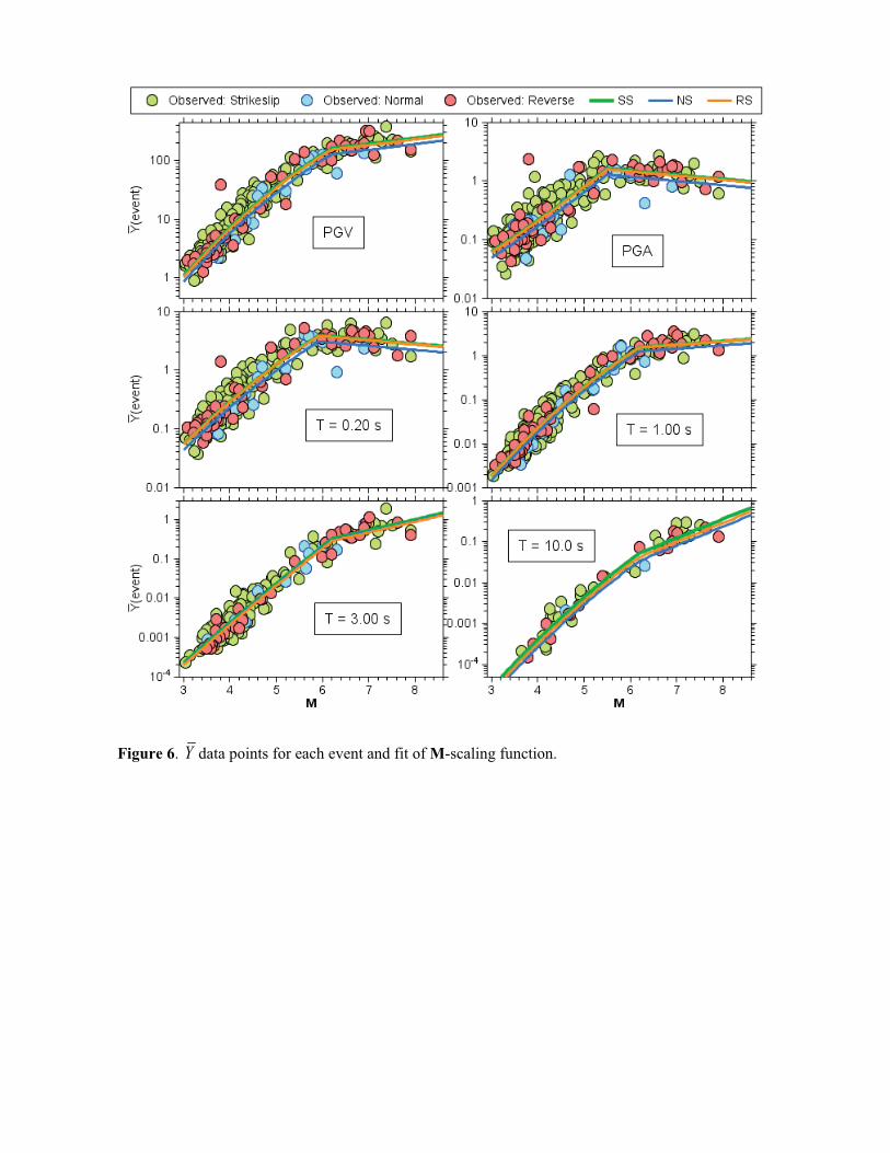
Figure 6. Y data points for each event and fit of M-scaling function.

Figure 7. Median trends of proposed GMPEs as compared to BA08�, as a function of distance for strike-slip earthquakes and 30 760 m/sSV � . The BA08� values have been adjusted to RotD50 using the ratios RotD50/GMRotI50 in Boore [2010] (maximum adjustment of 1.06 for T&=&10 s).

Figure 8. Variation of median predicted PSA versus period (T) for M 3, 4, 5, 6, 7, and 8 strike-slip earthquakes for RJB = 20 km and 30 200 m/sSV � and 760 m/s.

Figure 9. PSA vs JBR for two periods, 30 760 m/sSV � , and reverse-slip (RS) events, from equations derived with and without the 2008 M 7.9 Wenchuan earthquake.

Figure 10. Between-event residuals for CL1 (mainshock) events from Phase 3 analysis discriminated by fault type and CA vs non-CA regions. Note that there is almost no overlap in M for the CA and non-CA NS events, so it is difficult to judge possible bias for that condition.

Figure 11. Within-event residuals for regions identified as ‘Average Q’ (California, New Zealand,and Taiwan), ‘Low Q’ (Japan and Italy), and ‘High Q’ (China and Turkey). Also shown is the fit line per Eqn. (22) for RJB > 25 km.

Figure 12. Within event residuals against sediment depth differential 1z� along with proposed basin model. Results plotted are for southern California, San Francisco Bay Area, and Japan.
Figure 13. CL2 event term differential �# as function of CL1 magnitude (including binned means and their 95% confidence intervals). Results show no systematic offsets from zero, implying no increasing level of misfit of CL2 ‘children’ events as compared to their ‘parent’ CL1 event.

Figure 14. Event term variation with depth to top of rupture (Ztor) for M $�*�`{'�� ��`{|���� ���(including binned means and their 95% confidence intervals). Results show no significant offset from zero or trend, indicating lack of dependence of ground motion residuals on rupture depth.
Figure 15. Binned standard deviation terms and their 95% confidence intervals from Phase 3 analysis showing: (a) Between-event standard deviation ! against M; (b) within-event standard deviation "against RJB for M > 5.5, and (c) " against VS30 for M > 5.5 and RJB < 80 km. Lines in the figures represent model fits per Eqns. (1) to (9).

Figure 16. Comparison of the standard deviation terms in the BSSA14 GMPEs for 5.5�M ,80 kmJBR � and VS30 > 300 m/s with the M- and JBR -independent standard deviations from BA08.
Related Documents