Next part of course: CLASSICAL DYNAMICS - |LASP|CU …lasp.colorado.edu/~cranmer/ASTR_5120_2016/LecNotes/... · Next part of course: CLASSICAL DYNAMICS ... Newton’s 2nd law is derivable

Next part of course: CLASSICAL DYNAMICS

Gravity is important to all fields of astronomy & astrophysics.

Gravitational “celestial mechanics” is applicable over ∼20 orders of magnitude

in size scale: from comets (1 km) to galaxy superclusters (100 Mpc)!

We’ll start with mutual gravitation of small numbers of bodies (mainly

N = 2, 3).

Then we’ll extend our earlier studies of statistical mechanics and collisions to

systems of N ≫ 1 mutually gravitating bodies.

=⇒ Lots of similar concepts as before... Boltzmann equation, etc. ⇐=

Even without collisions, the N ≫ 1 body problem is non-trivial; i.e., what isthe motion of a “test particle” in a smooth gravitational potential Φ(r) causedby millions of other particles?

8.1

Calculus of Variations (all of it I hope you’ll ever need!)

A bit of pure math to start, but you’ll soon see that the physics applicationsare profound! Consider a 3D “trajectory” of a particle x(t), which we

examine between times t1 ≤ t ≤ t2.

Later we’ll define a functional called the Lagrangian, which may depend on

position x(t), velocity x(t), and time itself:

L [x(t), x(t), t] (leave it general for now) .

Let’s also define the path integral

I ≡∫ t2

t1

dt L [x(t), x(t), t] .

With L and x specified, I is just a scalar number.

Our goal will be to find the one (unique?) trajectory x(t) that causes the value

of I to be a local extremum (i.e., either minimum or maximum) compared toall neighboring trajectories.

Binney & Tremaine (§B.7) derive this one way; I’ll follow Marion’s ClassicalDynamics book.

We parameterize a given set of

“neighbor trajectories” as

x(t) = x0(t) + αx1(t)

and we fix the endpoints at t1 & t2,

x1(t1) = x1(t2) = 0 .

(We could “fill the space” around x0(t) by specifying any number of unique x1

perturbations, but let’s just look at one at a time.)

Anyway, we’d like to know how to specify the constraint that I(α) must have

an extremum at α = 0:(∂I

∂α

)

α=0

= 0 (for all possible x1’s) .

8.2

We’ll see that this puts constraints on the evolution of L.

We evaluate the α derivative by noting that the integration limits are fixed,so ∂/∂α affects only the integrand. Use chain rule:

∂I

∂α=

∫ t2

t1

dt

[∂L∂x

· ∂x∂α

+∂L∂x

· ∂x∂α

+∂L∂t

∂t

∂α

]

and we know

∂x

∂α= x1

∂x

∂α=

d

dt

(∂x

∂α

)

= x1

∂t

∂α= 0

where the last one can be seen by realizing that the α parameter is really justa function of space, not time.

Thus,∂I

∂α=

∫ t2

t1

dt

[

x1 ·∂L∂x

+ x1 ·∂L∂x

]

.

The 2nd term can be integrated by parts. Look at one Cartesian component at

a time: ∫ t2

t1

dt∂L∂x

dx1

dt=

[∂L∂x

x1

]t2

t1

−∫ t2

t1

dtd

dt

(∂L∂x

)

x1

and the 1st term on RHS = 0 because x1(t1) = x1(t2) = 0. Thus,

∂I

∂α=

∫ t2

t1

dt

x1 ·[∂L∂x

− d

dt

(∂L∂x

)]

Even though α doesn’t appear explicitly, this still formally depends on it (sincex & x depend on α). However, we want to evaluate (∂I/∂α)α=0.

Thus, we can realize that when we write x, we’re really referring to the

“central” trajectory x0.

Since x1 is a completely arbitrary perturbation, we see the only way to make

(∂I

∂α

)

α=0

= 0 is to require∂L∂x

=d

dt

(∂L∂x

)

everywhere along the trajectory.

This is the Euler–Lagrange (E–L) equation.

. . . . . . . . . . . . . . . . . . . . . . . . . . . . . . . . . . . . . . . . . . . . . . . . . . . . . . . . . . . . . . . . . . . . . . . . . . . . . .

8.3

Historically, many people realized that Nature seems to always want tominimize the “action” (i.e., time-integrated energy along a path) in a system.

Hero of Alexandria (∼50 AD) −→Fermat, Leibniz, Euler, Maupertuis, Lagrange (1700s) −→Hamilton, who unified classical dynamics (quote from Marion):

...and you know that Feynman took it even further, into quantum mechanics.

(FYI: In all cases we’ll encounter, the “extrema” are all minima.)

The relevant functional L is called the Lagrangian of the particle:

L(x, x) ≡ K(x) − U(x, x)

where the kinetic energy K depends only on x (velocity).

We’ll tend to encounter conservative force fields, for which the potentialenergy U is a function only of position x.

Consider a force derivable from a potential energy: F = −∇U .What does the E–L equation imply?

L = K − U =1

2m|x|2 − U(x) so

∂L∂x

= −∇U

and also,

K =m

2

(x2 + y2 + z2

) ∂K

∂x= mx , etc., so

∂L∂x

= mx .

8.4

Thus,∂L∂x

=d

dt

(∂L∂x

)

=⇒ −∇U = mxF = ma !

Newton’s 2nd law is derivable from Hamilton’s principle.

. . . . . . . . . . . . . . . . . . . . . . . . . . . . . . . . . . . . . . . . . . . . . . . . . . . . . . . . . . . . . . . . . . . . . . . . . . . . . .

Advantages of Lagrangian dynamics:

• L is a scalar, whereas forces & momenta (in the traditional “equation of

motion”) are vectors.

• Sometimes it’s difficult to specify the full list of forces acting on a body(including nebulous “forces of constraint”). Not needed here!

• This works even for non-Cartesian coordinates & non-inertial frames.In fact, for an N -dimensional system, if you can uniquely define some

other set of generalized coordinates,

qi = qi(x1, x2, . . . , xN)qi = qi(x1, x2, . . . , xN ; x1, x2, . . . , xN)

i = 1, 2, . . . , N

then you can go through the chain rule to show that

∂L∂q

=d

dt

(∂L∂q

)

is valid, too,

even if the q’s do NOT all have units of length!

Thus, the E–L equation is the same in all coordinate systems.

Aside: There’s neat symmetry if we also define a generalized momentum,

p =∂L∂q

(which can be verified from the full expression for K)

so that the E–L equation can be written as: p =∂L∂q

.

Soon, we’ll look at 2 examples of generalized coordinates:

• spherical coordinates (r, θ, φ) for relative motions between two bodies,

• rotating-frame coordinates, which let us derive the centrifugal & Coriolisforces from the E–L equation.

8.5

First, though, there are 2 important general principles we can PROVE asconsequences of symmetry. (≡ Noether’s theorem)

(1) Energy conservation: Consider a closed system, for which

∂L∂t

= 0 i.e., L doesn’t care about absolute time t .

The total derivative with respect to time can be written

dLdt

=∂L∂x

· x +∂L∂x

· x = x · d

dt

(∂L∂x

)

︸ ︷︷ ︸

from E–L

+ x ·(∂L∂x

)

Thus, from the chain rule,dLdt

=d

dt

(

x · ∂L∂x

)

which can be rearranged tod

dt

(

L − x · ∂L∂x

)

= 0

and the quantity in parentheses is a constant. Call it the Hamiltonian:

H ≡ x · ∂L∂x

− L = constant .

However, if we think back to the definition of the Lagrangian, and assume

U = U(x), we see that

x · ∂L∂x

= m|x|2 = 2K , so H = 2K − (K − U) = K + U

i.e., total energy is conserved as a consequence of time invariance.

(2) Momentum conservation: A closed system ought to also be invariant

to absolute translations (of the entire system) in space;

i.e., L should remain fixed if we replace x −→ x+ δx,

where δx is a fixed (small?) displacement.

With that, L should −→ L+ δL, via Taylor expansion,

δL =∂L∂x

· δx +∂L∂x

· δx

8.6

However, if the displacement is fixed, δx =d

dt(δx) = 0 ,

and we want to also specify δL = 0 . Thus,

∂L∂x

· δx = 0 , so for arbitrary δx,∂L∂x

= 0 .

From the E–L equation, this means

d

dt

(∂L∂x

)

= 0 , so∂L∂x

= constant .

Lastly, we know∂L∂x

= mx = p

so linear momentum is conserved as a consequence of spatial(translational) invariance.

Very similarly, we could also show that angular momentum is conservedas a consequence of rotational invariance, i.e., that

L = r× p = constant

for a closed system like this.

8.7

Central Force Motion: The Two-Body Problem

We’ve already thought about this a bit (Coulomb collisions).

The gravitational force is similar enough to the electrostatic force, that it

simplifies things to go into center-of-mass (CM) coordinates:

Recall: R =m1r1 +m2r2m1 +m2

r = r1 − r2

Here, let’s take advantage of the fact that U = R doesn’t change when 2

particles interact with one another.

Going fully into the CM frame (in which R = constant ≡ 0),

m1r1 +m2r2 = 0 =⇒ r1 = +

(m2

m1 +m2

)

r , r2 = −(

m1

m1 +m2

)

r .

With this, kinetic energy can be simplified. We write the LagrangianL = K − U , where for an N -body system, K is a sum over all N bodies, and

U is a sum over all N(N − 1)/2 unique pairs.

For this system,

L =

1

2m1|r1|2 +

1

2m2|r2|2

− U(r)

=1

2m|r|2 − U(r) where m = m12 =

m1m2

m1 +m2

and this reduces the 2-body problem to an equivalent 1-body problem.

Once we know the solution of r(t) for a “particle” of mass m, we can convertback to r1(t) & r2(t) for the real particles.

We do know more about the form of U(r), but let’s hold off writing it down.For now, note that it’s only a function of r = |r2|1/2.. . . . . . . . . . . . . . . . . . . . . . . . . . . . . . . . . . . . . . . . . . . . . . . . . . . . . . . . . . . . . . . . . . . . . . . . . . . . . .

What can we learn about this equivalent 1-body system? We can take

advantage of the fact it’s a “closed system” to use the conservation lawsdefined above:

(1) Linear momentum: The system’s total p = m1v1 +m2v2 ∝ R = 0,

so its conservation is not that interesting.

8.8

(2) Angular momentum: If L = r× p = constant, this means that both r& p remain ⊥ to a vector that’s fixed in time & space.

Thus, both r & p are always coplanar.

(I think we knew this already, intuitively, from Coulomb collisions...)

Thus, we can write everything in 2D polar coordinates (r, θ):

L =1

2mv2 − U(r) =

1

2m(

r2 + r2θ2)

− U(r)

where r & θ are our generalized coordinates (q1 & q2).

What does the Euler–Lagrange equation tell us for the θ coordinate?

∂L∂θ

=d

dt

(∂L∂θ

)

= 0

LHS = 0 because L doesn’t depend explicitly on θ. This means

∂L∂θ

= mr2θ = constant ≡ ℓ

which is essentially the magnitude of the system’s total angular momentum.

(3) Energy: This is assured for a closed system like this, so

E = K + U =1

2mr2 +

ℓ2

2mr2+ U(r) = constant .

Thus, we have two constants of motion: E and ℓ.

. . . . . . . . . . . . . . . . . . . . . . . . . . . . . . . . . . . . . . . . . . . . . . . . . . . . . . . . . . . . . . . . . . . . . . . . . . . . . .

Aside: We now know enough to derive Kepler’s 2nd law.(Strangely, it’s more fundamental than the 1st!)

Define the area A swept out by the position vector r of the particle’s path (inthe CM frame) between time t and t+ dt :

8.9

For very short times, r(t) ≈ r(t+ dt), so the triangle has area

dA =1

2r(r dθ) =

1

2r2dθ . (assuming dθ ≪ 1)

Thus,dA

dt=

1

2r2dθ

dt=

1

2r2θ =

ℓ

2m= constant .

and this is exactly Kepler’s 2nd law: planets sweep out “equal areas over equaltimes.”

Interestingly, it doesn’t depend on the orbits being of any particular shape, or

even on U(r) having any particular form.

. . . . . . . . . . . . . . . . . . . . . . . . . . . . . . . . . . . . . . . . . . . . . . . . . . . . . . . . . . . . . . . . . . . . . . . . . . . . . .

Equations of Motion for the Two-Body Problem

Our goal is a complete solution: i.e., r(t) and θ(t). In general, that is not

trivial, but we can bite off some pieces...

There are several ways to proceed. Right now, let’s just look at theconsequences of energy conservation.

Solve E = constant for r and we get a differential equation:

r =dr

dt=

√

2

m

[

E − U(r)− ℓ2

2mr2

]

=

√

2

m

[

E − V (r)]

where one often sees the effective potential

V (r) = U(r) +ℓ2

2mr2

as the sum of U(r) and a centrifugal potential (corresponding to what somecall a “fictitious force”).

8.10

Assuming we know the constants E & ℓ and the form of U(r), we could:

• Solve for dt & integrate to get t(r).

• Invert the solution to get r(t).

• Integrate the definition of ℓ to get θ(r) → θ(t).

In general, this needs to be done numerically, so we’ll put a pin in thisapproach for now.

Note also that only for some forms of U(r) do there exist “closed” orbits – i.e.,paths for which r(t) returns to its original value exactly when one loops around

a full 2π radians in θ.

Bertrand (1873) proved that there exist only two forms for which ALL orbits

are closed:

U(r) = −k

r(gravity) or U(r) = 1

2kr2 (simple harmonic oscillator)

How can we learn more? A useful alternate approach – which will help us learnabout the range of possible geometric shapes for orbital paths – is to use the

E–L equation for the r coordinate:

∂L∂r

=d

dt

(∂L∂r

)

mrθ2 − ∂U

∂r=

d

dt(mr) = mr

Or, after some rearranging,

m(

r − rθ2)

= −∂U

∂r≡ F (r) (RHS: the “force law”) .

We could simplify this by using ℓ = mr2θ and f = F/m, to get

r = f(r) +ℓ2

m2r3(1D equation of motion).

However, there is a popular change of variables (u = 1/r) that lets us write

this as a simpler 2nd order ODE for the orbit shape u(θ).

8.11

Using:du

dθ= − 1

r2dr

dθ= − r

r2 θ= −mr

ℓ(with ℓ = mr2θ)

and so on for d2u/dθ2, we eventually get

d2u

dθ2+ u = − m

ℓ2u2F (u) Binet’s equation .

This can be used in two ways:

• If we know F , solve the differential equation for the orbit.

• If we know the orbit, easily solve for F .

Doing the former is straightforward if we (finally!) specify a classical

gravitational potential:

U(r) = −Gm1m2

r= −γ

r=⇒ F (r) = − γ

r2= −γu2

and thus the RHS of Binet’s equation is a constant.

If we perform yet another change of variables,

y = u − mγ

ℓ2=⇒ d2y

dθ2+ y = 0

whose solution is a sinusoid. In general we can write

y(θ) = y0 cos(θ − θ0) which has 2 constants of integration.

Converting back to real units, we see: r(θ) =λ

1 + e cos(θ − θ0)

which are conic sections, with one focus at the origin. The 2 constants are

λ =ℓ2

mγ(semi-latus rectum; “orbit parameter”) e =

ℓ2 y0mγ

(eccentricity)

Note: λ tells us the overall spatial scale of the orbit, while e tells us moreabout its shape.

8.12

If we took this solution, substituted into energy conservation,

E =1

2mr2 +

ℓ2

2mr2− γ

r

(

using r =dr

dθθ

)

we’d be able to solve for e as a function of total energy:

e =

√

1 +2Eℓ2

mγ2=

√

1 +2λE

γ

What do the orbits look like... and how does E compare to V (r) ?

e > 1 E > 0 hyperbola (v > 0 as r → ∞)

e = 1 E = 0 parabola (v = 0 as r → ∞)0 < e < 1 Vmin < E < 0 ellipse

e = 0 E = Vmin circle (r = λ)e < 0 E < Vmin not allowed (r2 < 0, imaginary velocity!)

where it’s straightforward to show that

rmin =λ

1 + eand Vmin = −mγ2

2ℓ2= − γ

2λ.

Note that the plot for V (r) is only for a single value of ℓ. There’s really a whole

family of V (r, ℓ) for all possible orbits between 2 bodies of known masses.

8.13

Kepler himself thought a lot about the elliptical case (1st law).

a =γ

2|E| = semi-major axis

b =ℓ

√

2m|E|= semi-minor axis

Area = πab ,b

a=√

1− e2 , λ =b2

a

The orbit around one focus ranges between the apsides:

periapsis / pericenter / perigeeapapsis / apocenter / apogee

rmin = a(1− e) = λ/(1 + e)rmax = a(1 + e) = λ/(1− e)

. . . . . . . . . . . . . . . . . . . . . . . . . . . . . . . . . . . . . . . . . . . . . . . . . . . . . . . . . . . . . . . . . . . . . . . . . . . . . .

We can also derive Kepler’s 3rd law by recalling the 2nd law:

dt =2m

ℓdA .

Both sides can be integrated over an exact period:

t = 0 → PA = 0 → πab

Thus, P =2m

ℓπab =

2m

ℓπa3/2

√λ =

2m

ℓπa3/2

√

ℓ2

mγ.

Kepler squared both sides. The ℓ’s cancel, and we see that

P2 =

(4π2m

γ

)

a3

which isn’t quite Kepler’s 3rd law (i.e., the square of a planet’s period is

proportional to the cube of its semimajor axis), because the term inparentheses isn’t constant. It depends on planet mass. Writing it in full:

P2 =

(4π2

m1m2

(m1 +m2)Gm1m2

)

a3

and for the solar system, Mtot = (m1 +m2) = M⊙ +mplanet ≈ M⊙.

The 3rd law is only approximately true, but it’s pretty close.

8.14

For circular orbits, r = a, and astronomers tend to write it as

Ω =2π

P =

√

GMtot

r3∝ r−3/2 .

. . . . . . . . . . . . . . . . . . . . . . . . . . . . . . . . . . . . . . . . . . . . . . . . . . . . . . . . . . . . . . . . . . . . . . . . . . . . . .

We haven’t quite solved the full Kepler problem completely, since we still don’t

know the detailed time dependence r(t) & θ(t).

We could have integrated Kepler’s 2nd law for times other than P . Noting the

proportionality,

t

P =A(θ)

πab=

1

πab

∫ θ

0

12r2dθ′ =

λ2

2πab

∫ θ

0

dθ′

(1 + e cos θ′)2

(taking θ0 = 0). Even for an ellipse, it’s doable, but nasty:

2πt

P = 2 tan−1

(√

1− e

1 + etan

θ

2

)

− e√1− e2 sin θ

1 + e cos θ.

We’ll consider that knowing t(θ) is equivalent to knowing θ(t), since it’s a

single-valued function that can be tabulated numerically and “inverted” vialookup-table interpolation.

However, from the 1700s to the 1900s, a HUGE amount of effort was spent toinvert it analytically. I won’t go into Kepler’s equation (which depends on

θ-like quantitites called the “mean anomaly” & “eccentric anomaly”) and isprobably still taught in celestial mechanics classes.

. . . . . . . . . . . . . . . . . . . . . . . . . . . . . . . . . . . . . . . . . . . . . . . . . . . . . . . . . . . . . . . . . . . . . . . . . . . . . .

There’s a family of interesting physics problems involving making changes toan elliptical (or circular) orbit.

Two ways to do it:

(a) impulsive “∆v”(b) gradual gas drag

(E can go ↑ or ↓).

To make any progress working out the numbers, we need to examine some

additional consequences of energy conservation:

E =1

2mv2 − γ

r=⇒ v2 =

γ

m

(2

r+

2E

γ

)

8.15

For an elliptical orbit, it’s straightforward to show that

v2 =γ

m

(2

r− 1

a

)

= GMtot

(2

r− 1

a

)

the “vis–viva” equation.

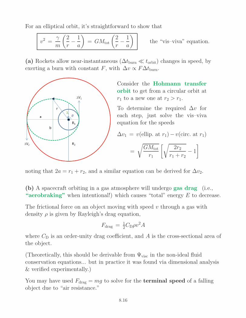
(a) Rockets allow near-instantaneous (∆tburn ≪ torbit) changes in speed, byexerting a burn with constant F , with ∆v ∝ F∆tburn.

Consider the Hohmann transfer

orbit to get from a circular orbit atr1 to a new one at r2 > r1.

To determine the required ∆v foreach step, just solve the vis–viva

equation for the speeds

∆v1 = v(ellip. at r1)− v(circ. at r1)

=

√

GMtot

r1

[√2r2

r1 + r2− 1

]

noting that 2a = r1 + r2, and a similar equation can be derived for ∆v2.

(b) A spacecraft orbiting in a gas atmosphere will undergo gas drag (i.e.,“aerobraking” when intentional!) which causes “total” energy E to decrease.

The frictional force on an object moving with speed v through a gas withdensity ρ is given by Rayleigh’s drag equation,

Fdrag = 12CDρv

2A

where CD is an order-unity drag coefficient, and A is the cross-sectional area ofthe object.

(Theoretically, this should be derivable from Ψvisc in the non-ideal fluid

conservation equations... but in practice it was found via dimensional analysis& verified experimentally.)

You may have used Fdrag = mg to solve for the terminal speed of a fallingobject due to “air resistance.”

8.16

The corresponding loss of kinetic energy is

v ·

mdv

dt= −Fdrag

=⇒ dE

dt= −CDρv

3A

An initially circular orbit will slowly decay. The drag is exerted ∼constantlyaround the orbit, and

E = Vmin = −GMtot

2r=⇒ r = −GMtot

2E=

GMtot

2|E|and decay makes E more negative. |E| ↑, so r ↓.

An initially elliptical orbit (around a body with an atmosphere) will

circularize, then decay. The strongest drag is at pericenter, because:

• ρ drops off exponentially with r

• v is highest at smallest r (vis–viva).

This is like an inverse Hohmann ∆v (i.e., pointing rockets in the oppositedirection of the orbit), and the lower E will result in the “next” orbit being a

lower-e ellipse with the same r1.

Circularization is important in close binary star systems, too.

For satellites, though, there’s great practical interest in this problem, becauseit’s a confluence of money (how long will my valuable satellite live?) and risk

(when & where will it crash?).

Also, ρ in Earth’s upper atmosphere depends on solar activity, sospace weather prediction is needed to model the long-term effects.

. . . . . . . . . . . . . . . . . . . . . . . . . . . . . . . . . . . . . . . . . . . . . . . . . . . . . . . . . . . . . . . . . . . . . . . . . . . . . .

Another interesting application of gas drag: planetary migration.

“Hot Jupiter” exoplanets were discovered in 1995, but their formation is apuzzle. It’s easy to form gas giants outside the “snow line” (∼3 AU for the

Sun, where it’s cold enough for dust grains to condense), but these planets arewell inside it.

8.17

Maybe they formed at large distances, then migrated inwards. How?

• Large-angle scattering in close encounters? (rare)

• Viscous drag with disk gas (preferred model?)

As the planet plows through the disk, it experiences drag with neighboringparcels of gas:

Coupling with

inner, higher-Ωouter, lower-Ω

gas

speeds upslows down

the planet.

Which wins? Depends on disk ρ(r, φ): more gas → more friction.

Low-mass planets: the latter tends to win. Planets tend to lose L (and/or E)

& migrate inwards.

High-mass: the planet’s gravity clears out a gap in the disk, so it feels ∼no

local drag force. But it’s an accretion disk, so everything gets brought in ⇒planet tends to migrate inwards.

How fast does it occur? Assume a diffusion timescale: tmig ∼ R2

ν

where the viscosity can be given by Shakura & Sunayev’s α model...

ν ∼ αH2Ω H = disk vertical scale height, α ∼ 0.01.

Thus, tmig ∼ 1

α

(R

H

)2√

R3

GM∗

and for H/R ∼ 0.1, M∗ ∼ M⊙, and R = 1–5 AU, we get tmig ∼ 103–104 years.

This is much shorter than disk lifetimes of ∼106 years.

8.18

What stops the migration (i.e., prevents it from colliding with star)?

• Disk is truncated by star’s strong magnetic field?

• Tidal interactions with star, once it comes very close?

• If planet formed “late,” disk may dissipate before migration done?

• Other planets may have paved the way; ate up disk gas?

Maybe “super-earths” are failed hot Jupiters, whose migration was halted?

Beyond elliptical orbits

Later we’ll look in more detail at gravitational interactions in N -body systems

(similar to Coulomb collisions in plasmas), so for now, we’ll postpone talkingabout hyperbolic (E > 0) orbits.

. . . . . . . . . . . . . . . . . . . . . . . . . . . . . . . . . . . . . . . . . . . . . . . . . . . . . . . . . . . . . . . . . . . . . . . . . . . . . .

Many other applications in astrophysics depend on the special case of

parabolic (E = 0) orbits: e.g.,

• star formation (infall accretion of mass from large distances)

• “single apparation” comets coming in from the Oort cloud

• the lowest-energy way to do spacecraft orbit insertion (“capture orbit”).

Consider the accretion problem. A point-mass chunk of interstellar material(dust grain? planetesimal?) falls in with E = 0, and thus zero kinetic energy

at r → ∞.

Will the parcel impact the star?

For angular momentum conservation,

ℓ = mr2θ = constant

and for e = 1, the parabolic path is

r(θ) =2rmin

1 + cos θ.

At the pericenter, θ = 0, and...

8.19

j =ℓ

m= r2

dθ

dt= r|vθ| = r|v| since, here, the motion is all vθ.

The vis–viva equation is easy to solve for E = 0, and

|v| =√

2GMtot

rand thus j =

√

2GMtotrmin is a constant of motion ,

with r(θ) =j2

GMtot(1 + cos θ)rmin =

j2

2GMtot

and the parcel will impact the newly-forming star if rmin ∼< R∗.

However, in the ISM, most parcels have rmin ≫ R∗.

Also, it’s clear that there’s never just oneparcel... There are really a huge number of

them coming in at all angles α (0→2π).

...where the star’s equatorial plane is

defined as the plane ⊥ to the net L vectorof the star + all other gas in the system.

If parcels are coming from above and below, they’ll collide/collect in theequatorial plane.

Here, θ = ±π

2i.e., cos θ = 0 , so req = 2 rmin =

j2

GMtot

.

When parcels collect at req, the gas will form a shock, and the orbital motionwill be decelerated.

For a parcel that starts at a distance D0 with angular velocity Ω0,

j0 = r2θ = Ω0D20 cosα

and since j is constant, we can solve for what happens at θ = π/2 and r = req

req =Ω2

0D40 cos

2 α

GM∗

8.20

For a maximum value of cosα ≈ 1, and

Ω0 ∼ 10−15 rad/s (local galactic shear)D0 ∼ 0.1 pc (typical GMC core fragment)

M∗ ∼ 1 M⊙ (typial protostar)

we get req ≈ 4 AU

as a representative radial extent of an accretion disk.

. . . . . . . . . . . . . . . . . . . . . . . . . . . . . . . . . . . . . . . . . . . . . . . . . . . . . . . . . . . . . . . . . . . . . . . . . . . . . .

The parabolic orbit (E ≈ 0) is always “on the edge” of either capture or

escape. It’s also possible to use gravity to make small nudges, as in...

The Gravitational Slingshot Effect

Consider a spacecraft moving with speed v, approaching a planet orbiting theSun with speed U .

In the planet’s frame, the parabolic flyby results in only a tiny net change inthe spacecraft’s speed. The spacecraft gains some p; planet loses some.

However, in the inertial frame, the spacecraft has “gained” speed 2U .(It can also lose 2U , if it approaches as the planet recedes...)

The momentum of the entire system is conserved, but the spacecraft is a tiny

contributor to that total.

Similar to the terrestrial analogy of a tennis ball being thrown at an

approaching wall... it bounces back faster.

8.21