WORKING PAPER 2008-10 REPA Resource Economics & Policy Analysis Research Group Department of Economics University of Victoria Corruption, Development and the Curse of Natural Resources Shannon M. Pendergast, Judith A. Clarke and G. Cornelis van Kooten July 2008 Copyright 2008 by S.M. Pendergast, J.A. Clarke and G.C. van Kooten. All rights reserved. Readers may make verbatim copies of this document for non-commercial purposes by any means, provided that this copyright notice appears on all such copies.

Welcome message from author
This document is posted to help you gain knowledge. Please leave a comment to let me know what you think about it! Share it to your friends and learn new things together.
Transcript
WORKING PAPER 2008-10
REPA
Resource Economics & Policy Analysis
Research Group
Department of Economics University of Victoria
Corruption, Development and the Curse of Natural Resources
Shannon M. Pendergast, Judith A. Clarke
and G. Cornelis van Kooten
July 2008
Copyright 2008 by S.M. Pendergast, J.A. Clarke and G.C. van Kooten. All rights reserved. Readers may make verbatim copies of this document for non-commercial purposes by any means, provided that this copyright notice appears on all such copies.
REPA Working Papers:
2003-01 – Compensation for Wildlife Damage: Habitat Conversion, Species Preservation and Local Welfare (Rondeau and Bulte)
2003-02 – Demand for Wildlife Hunting in British Columbia (Sun, van Kooten and Voss) 2003-03 – Does Inclusion of Landowners’ Non-Market Values Lower Costs of Creating Carbon
Forest Sinks? (Shaikh, Suchánek, Sun and van Kooten) 2003-04 – Smoke and Mirrors: The Kyoto Protocol and Beyond (van Kooten) 2003-05 – Creating Carbon Offsets in Agriculture through No-Till Cultivation: A Meta-Analysis of
Costs and Carbon Benefits (Manley, van Kooten, Moeltne, and Johnson) 2003-06 – Climate Change and Forest Ecosystem Sinks: Economic Analysis (van Kooten and Eagle) 2003-07 – Resolving Range Conflict in Nevada? The Potential for Compensation via Monetary
Payouts and Grazing Alternatives (Hobby and van Kooten) 2003-08 – Social Dilemmas and Public Range Management: Results from the Nevada Ranch Survey
(van Kooten, Thomsen, Hobby and Eagle) 2004-01 – How Costly are Carbon Offsets? A Meta-Analysis of Forest Carbon Sinks (van Kooten,
Eagle, Manley and Smolak) 2004-02 – Managing Forests for Multiple Tradeoffs: Compromising on Timber, Carbon and
Biodiversity Objectives (Krcmar, van Kooten and Vertinsky) 2004-03 – Tests of the EKC Hypothesis using CO2 Panel Data (Shi) 2004-04 – Are Log Markets Competitive? Empirical Evidence and Implications for Canada-U.S.
Trade in Softwood Lumber (Niquidet and van Kooten) 2004-05 – Conservation Payments under Risk: A Stochastic Dominance Approach (Benítez,
Kuosmanen, Olschewski and van Kooten) 2004-06 – Modeling Alternative Zoning Strategies in Forest Management (Krcmar, Vertinsky and
van Kooten) 2004-07 – Another Look at the Income Elasticity of Non-Point Source Air Pollutants: A
Semiparametric Approach (Roy and van Kooten) 2004-08 – Anthropogenic and Natural Determinants of the Population of a Sensitive Species: Sage
Grouse in Nevada (van Kooten, Eagle and Eiswerth) 2004-09 – Demand for Wildlife Hunting in British Columbia (Sun, van Kooten and Voss) 2004-10 – Viability of Carbon Offset Generating Projects in Boreal Ontario (Biggs and Laaksonen-
Craig) 2004-11 – Economics of Forest and Agricultural Carbon Sinks (van Kooten) 2004-12 – Economic Dynamics of Tree Planting for Carbon Uptake on Marginal Agricultural Lands
(van Kooten) (Copy of paper published in the Canadian Journal of Agricultural Economics 48(March): 51-65.)
2004-13 – Decoupling Farm Payments: Experience in the US, Canada, and Europe (Ogg and van Kooten)
2004–14– Afforestation Generated Kyoto Compliant Carbon Offsets: A Case Study in Northeastern Ontario (Biggs)
2005–01– Utility-scale Wind Power: Impacts of Increased Penetration (Pitt, van Kooten, Love and Djilali)
2005–02 –Integrating Wind Power in Electricity Grids: An Economic Analysis (Liu, van Kooten and Pitt)
2005–03 –Resolving Canada-U.S. Trade Disputes in Agriculture and Forestry: Lessons from Lumber (Biggs, Laaksonen-Craig, Niquidet and van Kooten)
2005–04–Can Forest Management Strategies Sustain the Development Needs of the Little Red River Cree First Nation? (Krcmar, Nelson, van Kooten, Vertinsky and Webb)
2005–05–Economics of Forest and Agricultural Carbon Sinks (van Kooten) 2005–06– Divergence Between WTA & WTP Revisited: Livestock Grazing on Public Range (Sun,
van Kooten and Voss) 2005–07 –Dynamic Programming and Learning Models for Management of a Nonnative Species
(Eiswerth, van Kooten, Lines and Eagle) 2005–08 –Canada-US Softwood Lumber Trade Revisited: Examining the Role of Substitution Bias
in the Context of a Spatial Price Equilibrium Framework (Mogus, Stennes and van Kooten)
2005–09 –Are Agricultural Values a Reliable Guide in Determining Landowners’ Decisions to Create Carbon Forest Sinks?* (Shaikh, Sun and van Kooten) *Updated version of Working Paper 2003-03
2005–10 –Carbon Sinks and Reservoirs: The Value of Permanence and Role of Discounting (Benitez and van Kooten)
2005–11 –Fuzzy Logic and Preference Uncertainty in Non-Market Valuation (Sun and van Kooten) 2005–12 –Forest Management Zone Design with a Tabu Search Algorithm (Krcmar, Mitrovic-Minic,
van Kooten and Vertinsky) 2005–13 –Resolving Range Conflict in Nevada? Buyouts and Other Compensation Alternatives (van
Kooten, Thomsen and Hobby) *Updated version of Working Paper 2003-07 2005–14 –Conservation Payments Under Risk: A Stochastic Dominance Approach (Benítez,
Kuosmanen, Olschewski and van Kooten) *Updated version of Working Paper 2004-05 2005–15 –The Effect of Uncertainty on Contingent Valuation Estimates: A Comparison (Shaikh, Sun
and van Kooten) 2005–16 –Land Degradation in Ethiopia: What do Stoves Have to do with it? (Gebreegziabher, van
Kooten and.van Soest) 2005–17 –The Optimal Length of an Agricultural Carbon Contract (Gulati and Vercammen) 2006–01 –Economic Impacts of Yellow Starthistle on California (Eagle, Eiswerth, Johnson,
Schoenig and van Kooten) 2006–02 -The Economics of Wind Power with Energy Storage (Benitez, Dragulescu and van
Kooten) 2006–03 –A Dynamic Bioeconomic Model of Ivory Trade: Details and Extended Results (van
Kooten) 2006–04 –The Potential for Wind Energy Meeting Electricity Needs on Vancouver Island (Prescott,
van Kooten and Zhu) 2006–05 –Network Constrained Wind Integration: An Optimal Cost Approach (Maddaloni, Rowe
and van Kooten) 2006–06 –Deforestation (Folmer and van Kooten) 2007–01 –Linking Forests and Economic Well-being: A Four-Quadrant Approach (Wang,
DesRoches, Sun, Stennes, Wilson and van Kooten) 2007–02 –Economics of Forest Ecosystem Forest Sinks: A Review (van Kooten and Sohngen) 2007–03 –Costs of Creating Carbon Offset Credits via Forestry Activities: A Meta-Regression
Analysis (van Kooten, Laaksonen-Craig and Wang) 2007–04 –The Economics of Wind Power: Destabilizing an Electricity Grid with Renewable Power
(Prescott and van Kooten) 2007–05 –Wind Integration into Various Generation Mixtures (Maddaloni, Rowe and van Kooten) 2007–06 –Farmland Conservation in The Netherlands and British Columbia, Canada: A Comparative
Analysis Using GIS-based Hedonic Pricing Models (Cotteleer, Stobbe and van Kooten)
2007–07 –Bayesian Model Averaging in the Context of Spatial Hedonic Pricing: An Application to Farmland Values (Cotteleer, Stobbe and van Kooten)
2007–08 –Challenges for Less Developed Countries: Agricultural Policies in the EU and the US (Schure, van Kooten and Wang)
2008–01 –Hobby Farms and Protection of Farmland in British Columbia (Stobbe, Eagle and van Kooten)
2008–02 –An Economic Analysis of Mountain Pine Beetle Impacts in a Global Context (Abbott, Stennes and van Kooten)
2008–03 –Regional Log Market Integration in New Zealand (Niquidet and Manley) 2008–04 –Biological Carbon Sequestration and Carbon Trading Re-Visited (van Kooten) 2008–05 –On Optimal British Columbia Log Export Policy: An Application of Trade theory (Abbott) 2008–06 –Expert Opinion versus Transaction Evidence: Using the Reilly Index to Measure Open Space premiums in the Urban-Rural Fringe (Cotteleer, Stobbe and van Kooten) 2008–07 –Forest-mill Integration: a Transaction Costs Perspective (Niquidet and O’Kelly) 2008–08 –The Economics of Endangered Species Poaching (Abbott) 2008–09 –The Ghost of Extinction: Preservation Values and Minimum Viable Population in Wildlife
Models (van Kooten and Eiswerth) 2008–10 –Corruption, Development and the Curse of Natural Resources (Pendergast, Clarke and van
Kooten)
For copies of this or other REPA working papers contact: REPA Research Group
Department of Economics University of Victoria PO Box 1700 STN CSC Victoria, BC V8W 2Y2 CANADA
Ph: 250.472.4415 Fax: 250.721.6214
www.vkooten.net/repa This working paper is made available by the Resource Economics and Policy Analysis (REPA) Research Group at the University of Victoria. REPA working papers have not been peer reviewed and contain preliminary research findings. They shall not be cited without the expressed written consent of the author(s).

Corruption, Development and the Curse of Natural Resources
by
Shannon M. Pendergast
Judith A. Clarke
and
G. Cornelis van Kooten
Department of Economics University of Victoria
P.O Box 1700, Stn CSC Victoria, BC V8W 2Y2
Draft: March 7, 2008
Abstract
In 1995, Jeffrey Sachs and Andrew Warner found a negative relationship between natural
resources and economic growth, and claimed that natural resources are a curse. Their work has
been widely cited, with many economists now accepting the curse of natural resources as a well-
documented explanation of poor economic growth in some economies (e.g., Papyrakis and
ii
ii
Gerlagh, 2004; Kronenberg, 2004). In this paper, we provide an alternative econometric
framework for evaluating this claim, although we begin with a discussion of possible
explanations for the curse and a critical assessment of the extant theory underlying the curse. Our
approach is to identify natural resources that have the greatest rents and potential for exploitation
through rent-seeking agents. The transmission mechanism that we specify works through the
effect that rent seeking has on corruption and how that, in turn, impacts wellbeing. Our measure
of wellbeing is the Human Development Index, although we find similar results for per capita
GDP. While we find that resource abundance does not directly impact economic development,
we do find that petroleum resources are associated with rent-seeking behavior that negatively
affects wellbeing. Our regression results are robust to various model specifications and
sensitivity analyses.
Keywords: natural resource curse, petroleum resources, unbalanced panels and GMM estimation
JEL Categories: O12, Q32, Q34, O43, O47

Corruption, Development and the Curse of Natural Resources
1. Introduction
In the late nineteenth and early twentieth century, Britain and France gained economic
prosperity by exploiting the natural resources of their colonies. Britain benefited from gold and
diamond extraction in South Africa, and France from harvesting rubber and mining bauxite in
Guinea. During the nineteenth century, land was one of the most important natural resources, and
land abundant countries such as Canada, the United States and Australia had some of the highest
real wages in the world (Weil, 2005). Britain, Germany and the US relied heavily on coal and
iron ores deposits during their industrialization phases (Sachs and Warner, 1995). Indeed, some
developed countries still rely heavily on natural resources to this day (e.g., the forest sector
accounts for some 5% of all jobs in Canada). These examples suggest that natural resources
promote economic development.
History also tells us that natural resource abundance is not a requirement for economic
prosperity. Switzerland is one of the wealthiest countries in the world today, but its path to
economic prosperity depended on the financial and manufacturing sectors, not extraction of
natural resources. More recently, Hong Kong, Singapore, South Korea and Taiwan developed
despite a relative scarcity of natural resources. Nor does natural resource abundance guarantee
economic prosperity. South Africa and Venezuela possess abundant natural resources but neither
enjoys a high standard of living, as they are plagued by corruption, civil unrest and income
inequality. These examples suggest that natural resources have a negative influence on economic
development.
Cursory evidence suggests that natural resources are not a necessary condition for
2
economic development, nor are they a sufficient condition for development. However, when in
1995 Jeffrey Sachs and Andrew Warner found a negative relationship between natural resources
and economic growth, many economists accepted that natural resources might be an obstacle –
indeed, a curse – to economic development (e.g., Papyrakis and Gerlagh, 2004; Kronenberg,
2004). But not all economists agree. Despite widespread acceptance of the curse hypothesis,
there is significant contradictory evidence that suggests natural resource abundance may not
hinder economic outcomes (e.g., Sala-i-Martin and Subramanian, 2003).
So, are natural resources a curse or a blessing? In this paper, we evaluate this question by
developing a framework that differs somewhat from that used by others. We begin in section 2
by reviewing the extant literature, followed by a discussion of possible explanations for the
existence of the curse. Then, in section 3, we provide a theoretical discussion about how the
resource curse should be specified. In section 4, we develop an empirical model for evaluating
the validity of the resource curse hypothesis, presenting the findings in section 5. We end with
some concluding remarks.
2. Evidence For and Against the ‘Curse’ and Possible Explanations
In the resource curse literature, the most commonly cited work is by Sachs and Warner
(1995; also 1997a, 1997b, 1999, 2001), who found a negative relationship between the share of
primary exports in GDP and economic growth between 1970 and 1989. Although the cross
country regressions they estimated indicate a negative relationship between natural resources and
economic growth, the mechanism through which the resource curse operates is unclear. The
authors claim to provide evidence of the negative effect of resource abundance on growth, but
their measure of ‘abundance’ (share of primary exports in GDP) can better be interpreted as a
3
measure of ‘dependence’ (the degree to which the economy depends on natural resources for its
economic livelihood). To be fair, Sachs and Warner (1995) show that their results are robust to
alternative specifications of resource abundance, but each of these has its problems. Two of the
alternative measures they test (share of mineral production in GDP and fraction of primary
exports in total exports) are similar to their first measure in that they really capture resource
dependence, not resource abundance. (Similar results are found in Sala-i-Martin (1997), and
Sala-i-Martin, Doppelhofer and Miller (2003).) The authors’ third specification (land area per
person) does indeed constitute a measure of resource abundance, but, since not all land is the
same, it is a very imprecise measure of primary sector productivity, as the authors recognize.
Additional support for the resource curse hypothesis is found in Naidoo (2004), who
measures extraction of forest resources by using the area of forest cover that a country cleared
during the period 1960-1999. He finds a negative association between the liquidation of forest
resources and economic growth rates. Again, this measure may really reflect the degree to which
a country is dependent on natural resources. Countries that cleared a large proportion of their
forests in a given period may have done so out of necessity (there were no other feasible options
to earn income). Naidoo controls for the absolute size of a country (to distinguish large, resource
poor countries from small, resource rich ones), but fails to control for the impact of population
when measuring a country’s resource abundance.
Sala-i-Martin and Subramanian (2003) find that, upon controlling for institutional quality,
natural resources are not significantly related to economic growth. They also show that the effect
of natural resources depends on the particular ones being considered. Fuel and mineral resources
negatively impact institutions (and hence economic growth), but the relationships between
economic growth and other types of resources are generally found to be statistically insignificant.

4
This is a very important finding, because it suggests that the curse of natural resources may
really be a curse of particular natural resources.
Papyrakis and Gerlagh (2004) concur with these findings. Upon taking corruption,
investment, openness, terms of trade and schooling into account, they find natural resource
abundance to have a positive impact on growth. Focusing on these additional explanatory
variables may hold the key to unlocking the mystery of the resource curse. However, although
these authors claim to have found a connection between natural resource abundance and
economic growth, their measure of resource abundance (share of mineral production in GDP)
remains problematic. This variable measures resource intensity and not abundance, but, as shown
by Sala-i-Martin and Subramanian (2003), abundance of mineral and fuel resources may not
yield the same economic outcome as abundance of other natural resources.
Manzano and Rigobon (2001) build on Sachs and Warner’s model by re-estimating the
effect of natural resources on economic growth using panel data and alternative measures of the
non-resource side of the economy. Interestingly, in every specification they use, the negative
impact of the resource curse appears in their cross-sectional data, but is insignificant when they
estimate a fixed-effects panel data model.
The literature also provides a number of possible explanations for the natural resource
curse. We consider six possible explanations. First, the Dutch disease phenomenon historically
described the situation where a rise in the value of natural resource exports caused a country’s
real exchange rate to appreciate, thereby making it more difficult for that country to compete
internationally. An increase in natural resource exports could be caused by increases in export
commodity prices, or by an increase in the commodity export volume (perhaps due to the
discovery of new resources, as was the case in the Netherlands with the discovery of natural gas
5
in the late 1950s). Economists expect increased emphasis on primary sector production and
reduced attention to the secondary or manufacturing sector to have a negative impact on
economic growth (Kronenberg, 2004; Papyrakis and Gerlagh, 2004). More recently, the Dutch
disease explanation has placed less emphasis on exchange rate movements and more on
economic distortions that encourage growth of the primary sector at the expense of more
advanced sectors, such as manufacturing (Barbier, 2003). Further, volatility of commodity prices
could harm the domestic economy by creating uncertainty that reduces exports, trade and foreign
investment (Gylfason, 2001).
Second, Barbier (2003) points out that “any depreciation of natural resources must be
offset by investment in other productive assets” (p.263). However, he finds that in many
developing countries resource rents are not generally channelled into productive investments, but
are frequently dissipated through corruption, bureaucratic inefficiency and policies aimed at rent-
seeking interest groups. A major focus in this paper is on the relationship between natural
resources and rent seeking behavior.
Third, countries with abundant natural resources may have reduced incentives to invest in
human capital. Temporary wealth from resource sales may cause countries to under-estimate the
need to accumulate the human capital needed to foster long-term growth. There is some evidence
that public spending on education is negatively related to abundance of natural resources
(Gylfason, 2001).
Fourth, Gylfason (2001, 2002) considers how abundance of natural resources reduces
incentives to save and invest, thereby limiting physical capital formation and economic growth.
In his argument the demand for capital falls as owners of capital earn a higher share of output,
thus lowering real interest rates and reducing investment.

6
Fifth, there is an interesting and expansive literature that examines the relationship
between resource rents and civil war. Collier and Hoeffler (2004) argue that extortion of natural
resources provides an opportunity to finance rebellion. Lujala, Gleditsch and Gilmore (2005)
show how rebel groups have used resource rents to finance warfare and personal incomes;
resource rents provide income for corrupt governments while simultaneously making it more
desirable to hold political power. Further, existence of resource rents provides an incentive to
overthrow the government, while an abundance of natural resources creates opportunities for
looting and extortion that provide insurgents with the financial means to undertake rebellion.
Using logit regression to predict the outbreak of civil war, Collier and Hoeffler (2004)
find that the share of primary commodity exports in GDP is a significant predictor of conflict.
However, upon disaggregating commodity exports into various subgroups, only oil exports turn
out to be a significant predictor of conflict. Further evidence supporting this claim comes from
Fearon (2005), and from Lujala, Gleditsch and Gilmore (2005), who find a positive relationship
between diamond production and the incidence of civil war. The latter find, however, that this is
the case only for secondary diamonds that can be looted, while production of primary diamonds
(that cannot be looted) is negatively related to the incidence of civil war. Clearly, resource
characteristics and their ability to generate rents must be taken into account when investigating
the resource curse.
Finally, Sachs and Warner (2001) claim that the natural resource curse exists independent
of commodity prices, but others believe it is a result of commodity price volatility. For example,
Manzano and Rigobon (2001) argue that high commodity prices in the 1970s encouraged
resource-abundant developing countries to borrow heavily. When commodity prices dropped in
the 1980s, these countries were left with a large debt burden and a lower stream of resource rents
7
to service this debt. The resource curse disappears once this ‘debt-overhang’ problem is taken
into account (Manzano and Rigobon, 2001). Similar arguments relating to commodity price
volatility are made by Deaton (1999), Gelb (1988) and Auty (1993). Interestingly, Deaton shows
that commodity prices, while highly volatile, lack a distinct upward trend. If real commodity
prices do not grow over time, any country dependent on them will have difficulty achieving
long-run growth. Meanwhile, Collier and Goderis (2007) used a panel cointegration method to
show that commodity booms have positive short-term effects on output, but adverse effects in
the long run. However, these adverse effects are confined to non-agricultural commodities.
3. Defining the “Curse of Natural Resources”
While the curse of natural resources implies a negative relationship between natural
resources and wellbeing, it is well to ask how this relationship is defined. After all, natural
resource dependence might result in low levels of wellbeing (however wellbeing is interpreted),
or it might inhibit economic growth (of GDP or per capita GDP). Alternatively, abundance of
natural resources might lead to low wellbeing or inhibit growth. Each of these relationships
might operate through any one of the transmission mechanisms described above. While natural
resources might affect economic growth rates, a country with slow economic growth but a
relatively high standard of living cannot be considered cursed. Therefore, the most relevant
research question should relate to levels of wellbeing and not to economic growth rates.
Even more important, using economic growth to address the resource curse hypothesis
may result in spurious correlation between economic growth and natural resources. For example,
suppose abundance of natural resources is good for economic development. As countries
experience rising income levels, they tend to find that their economic growth rates decline.
8
Developed countries typically grow at relatively low, stable rates. Furthermore, they may find
slow, stable growth desirable and attempt to prevent their economies from growing too quickly
(to mitigate inflation, say). If natural resource abundance is good for economic development,
most resource abundant countries will be developed nations, currently experiencing relatively
slow but stable economic growth. In contrast, resource poor countries will tend to be less
developed nations, and may experience more volatile economic growth rates. Hence, regressing
economic growth rates on abundance of natural resources may lead to spurious correlation
between these two variables.
While natural resource dependence might prevent countries from achieving a high
standard of living, dependence on agricultural products can be easily accounted for by structural
change theories of economic development. These theories suggest that economic development
occurs as economies transition away from subsistence agriculture toward industrially diverse
manufacturing and service sectors (Todaro and Smith, 2002; Lewis, 1954). It is the transition
towards manufacturing and services that improve a country’s total productivity. If countries do
not make this structural transformation, and remain dependent on agriculture, it is unlikely that
they will have the means to achieve higher productivity and increased standards of living.
The relatively simple concept of ‘value-added’ can also explain how resource
dependence might inhibit economic development. Activities in the secondary and tertiary sectors
of the economy tend to add more value than activities in the primary sector. The process of
converting raw material into an automobile clearly adds more value than the process of
extracting those raw materials. Because the secondary and tertiary sectors of the economy create
more value added, economies with large secondary and tertiary sectors support higher standards
of living. Economies with large primary sectors (high dependence on natural resources as a

9
source of income) are not able to support these same standards of living. Virtually every country
that has experienced rapid productivity gains in the past two centuries has done so by
industrializing (Murphy, Shleifer and Vishny, 1989). The decreased importance of the primary
sector allowed these countries to enjoy higher living standards. In this case, the natural resource
curse seems to be a certainty, and researching it would not provide particularly novel insights.
Measuring Wellbeing and Resource Abundance
This only leaves the question of the relationship between resource abundance and levels
of wellbeing. How should we specify wellbeing? Modern development economists, such as
Amartya Sen, view development as a multi-faceted goal that can only be achieved holistically by
increasing material, physical and psychological wellbeing. The common indicators used to
measure these objectives include per capita GDP, the Gini coefficient (a measure of income
inequality), infant mortality rates, life expectancy, literacy rates, and rates of enrolment in
primary education. To address the resource curse hypothesis properly, therefore, the dependent
variable should be specified in a way that captures this multi-dimensional aspect. A popular
development index is the United Nations’ Human Development Index, which equally weights
income levels, health and education, but neglects the distribution of income. However, given that
reliable estimates of income inequality are only available for selected countries at certain times,
we employ both the Human Development Index (HDI) and GDP per capita to measure average
standards of living across countries, although our focus will primarily be on the former.
We also need a proper measure of resource abundance. Gylfason (2002) identifies three
possibilities: (i) the share of primary exports in total exports or share in GDP; (ii) the share of
primary production in employment; and (iii) the share of natural capital in national wealth.
10
However, each of these measures fails to capture the true notion of resource abundance. We
should think in absolute terms; for example, we could consider the absolute size of a country’s
inventory of natural resources, or natural resources per capita. To measure a country’s natural
resource abundance, we should not consider the size of its primary sector relative to the non-
primary ones. Resource production as a share of total goods and services production,
employment in the natural resource industry compared to other industries, or the value of natural
resources compared to the value of all of other assets can more accurately be described as
measuring the relative degree of resource dependence. The problem is that countries can have
abundant natural resources (in terms of available resources per capita) and not have resources
make up a large share of exports, employment or wealth. As a country develops other sectors of
its economy, the share of natural resources in exports, employment and wealth should fall. Thus,
it is important to distinguish between measuring natural resource abundance in relative terms
(relative to the size of other sectors of the economy) and absolute terms (available natural
resources per capita).
Of the measures proposed by Gylfason, measure (i) appears to be most commonly used to
study natural resources and economic growth. In their influential paper, Sachs and Warner
(1995) measure natural resource abundance using the ratio of primary product exports to GDP,
finding a negative relationship between natural resources and economic growth. However, the
use of this measure to model economic growth rates leads to endogeneity problems. Suppose that
the secondary and tertiary sectors of economies grow faster than the primary sector. In these
economies, the share of primary exports in GDP will decline over time, even if the primary
sector contributes positively to economic growth. Thus, economic growth is correlated with a
declining share of primary exports in GDP, leading to the conclusion that the primary sector is

11
negatively related to economic growth. Nonetheless, as long as the primary sector is growing, the
primary sector is actually contributing positively to economic growth. This is where the
distinction between natural resource abundance and natural resource dependence becomes very
clear. An abundance of natural resources may lead to positive economic growth, but if this
comes at the expense of the secondary and tertiary sectors of the economy, this natural resource
dependence may decrease economic growth.
Others have also pointed out various problems associated with measuring resource
abundance by the share of primary commodity exports to GDP (Lujala et al., 2005; de Soysa,
2002). De Soysa (2002) measures resource abundance in terms of available natural resources per
capita, similar to what is done in this study. We estimate available resource rents using per capita
measures of resource exports and resource production. The transformation of resource exports
and production into per capita terms is crucial in determining the extent to which resource rents
have the potential to increase average living standards in a given country. If resource exports
and/or production were measured in aggregate terms, then large countries with large populations
would appear resource rich, when, in fact, the potential for resource rents to impact overall
standards of living could be quite small. Similarly, small countries with modest populations
would appear resource poor, even if the available natural resources per capita were substantial.
Transforming aggregate natural resource exports and production into per capita terms creates a
measure of resource abundance that more accurately reflects the potential for resource rents to
impact average overall standards of living.
In this study, we consider only natural resources that are openly traded in the global
market economy, namely, agricultural resources (e.g., grain, coffee, tea, beef), forest resources
(e.g., pulp, lumber), fuel resources (e.g., coal, natural gas, crude oil), and ores and mineral
12
resources (e.g., gold, tungsten, diamonds). As noted in the foregoing discussion, early studies
treated all natural resources as relatively homogenous, whereas more recent studies indicate that
the validity of the natural resource curse clearly depends on how natural resources are delineated
(Sala-i-Martin and Subramanian, 2003; Collier and Hoeffler, 2004, 2005).
4. Framework for Evaluating the Natural Resource Curse
Discussions of the natural resource curse must begin by considering natural resource rent.
Resource rents consist of scarcity rents plus differential (or Ricardian) rents (van Kooten and
Folmer, 2004, pp.41-44). Scarcity rent refers to the difference between marginal revenue and
marginal production cost that can only come about as a result of the natural or policy-induced
scarcity of a resource. Differential rent, on the other hand, refers to the excess of the market
value of non-marginal units of in situ resources over and above current scarcity rents.
Differential rents are given by the area above the all factors variable resource supply curve and
below the cost of providing the marginal unit. Scarcity rent is then the difference between output
price and the marginal cost of providing the last unit multiplied by the amount of the resource
provided. Resource rents are greater for some natural resources than others. Agriculture is
unlikely to result in significant rents (with some exceptions), because agriculture is an annual
activity that requires inputs of labor and capital each year to extract any rent, and rent is mainly
of a Ricardian nature. There is a risk that output prices fall between the time of planting and
harvest, or that adverse weather leads to low yields or crop failure. Further, while the surplus
from agriculture can be a driver of economic development, rents in agriculture are generally too
small or spread over too many landowners, or both, to attract the attention of rent seekers. It is
not surprising, therefore, that the resource curse literature finds that “the inclusion or exclusion
13
of agriculture does not much alter the basic results” (Sachs and Warner, 2001, p.831).
Forest resources offer a potentially much more valuable surplus to rent seekers than is
generally available from agriculture. Large forest rents are feasible on some valuable sites of
mature standing timber. However, forests rents are very much smaller or insignificant if the costs
of tree planting and waiting for trees to mature are properly taken into account, as is the case
with plantation forests. In many regions where deforestation takes place, it occurs because, after
rents are captured through harvest, the land is more valuable in agriculture than growing trees. In
some countries, forestlands are publicly owned with governments having some success in
collecting related rents. Nonetheless, there are situations where illegal logging is rampant (e.g.,
Ukraine, Malaysia, Indonesia), because of the lucrative windfalls. In the resource curse literature,
forestry is generally included with all other resources, ignored entirely, or no distinction is made
between types of forest resources – natural forests that can generate large rents upon being
logged and plantation forests that generally support processing and manufacturing activities.
The extraction of fossil fuels (especially crude oil), copper, uranium, and other valuable
metals and minerals (especially diamonds and gold) has much greater potential to incite rent
seeking behavior. The reason is that extraction activities are spatially much more concentrated
than in forestry and agriculture, these activities generate much higher rents, and rent capture is
generally easier. Without proper property rights, enforcement of property rights and independent
courts, rent seeking leads to lawlessness and corruption to the detriment of the economy (De
Soto, 2000; Anderson and Hill, 2004). Resource rents are dissipated in a variety of ways that
include bribery in its various forms, spending on militias to protect the beneficiaries from other
rent seekers, transfer of wealth to private overseas bank accounts, investments in overseas stock
markets to the benefit of the ruling elite, and so on. The point is: The existence of resource rents
14
encourages rent seeking, corruption and behavior that are ultimately detrimental to economic
growth and development (Ades and Di Tella, 1999; Azfar, Young and Swamy, 2001). It is not
the natural resources that are the curse, but government failure that is the problem. Governments
do not define and enforce property rights, nor do they protect citizens from theft, which is
commonly carried out by agents of government. The literature on the resource curse often hints
at all this, but fails to expand on it in any formal way.1
If social institutions such as civil law and property rights exist, rent seeking and
corruption may not occur to the same degree. However, the relationship between rent seeking
and corruption and institutional quality is bi-directional. While well developed institutions may
reduce corruption, corruption may also reduce the quality of institutions.
Econometric Specification
To overcome problems associated with endogeneity between institutions and corruption/
rent seeking, we employ a systems regression model:
(1) yit = αit + β1 x1i + β2 x2it + ... + βK xKit + εit , i= 1, ...,N; t= 1, ...,Ti,
(2) cit = δit + γ1 z1it + + γ 2 z2it + ... + γM zMit + ξit , i= 1, ...,N; t= 1, ...,Ti.
Here yit is a measure of economic wellbeing (HDI or per capita GDP) of country i in period t; xkit
(k=1, …, K) are characteristics of country i that influence wellbeing; cit is control of corruption;
and zmit (m=1, …, M) are country- and time-specific factors that affect corruption. Our dataset is
an unbalanced panel, allowing for countries to contribute observations for different time periods;
1 Thus, Sachs and Warner (2001, p.48) state: “There is an inverse association between natural resource abundance and several measures of institutional quality”. But they make no effort to explain why, other than to point out that quality of institutional measures is less than desirable.

15
the total number of observations is denoted by n =∑=
N
1iiT . Regressors were chosen on the basis of
theory, empirical results from the literature, data availability and preliminary data analysis.
These are discussed further below. Regressor parameters, βk and γm, are assumed not to vary by
country or time period, whereas, in this general model, the intercept terms (αit and δit) are
permitted to change with both country and time. Specific assumptions for these intercept terms
are given below. The model’s errors, εit and ξit, are assumed to have mean zero with possible
heteroskedasticity of unknown form over i and t.
Our data are compiled from a variety of sources, although most indicators come directly
or indirectly from the World Bank. (Detailed definitions of the variables and data sources are
provided in Appendix A.) We have 366 (=n) observations covering 102 (=N) countries at
possibly four points in time – 1998, 2000, 2002 and 2004. A list of countries is provided in
Appendix B, while descriptive statistics for the variables are provided in Table 1. Monetary
values are in constant 2000 US$. Forest output is measured in cubic meters of roundwood.
As a dependent variable in equation (1), we employ the HDI, which is a weighted index
comprised of income (measured by purchasing power parity GDP per capita), health (measured
by life expectancy at birth), and education (measured by adult literacy and gross school
enrolment rate). As an alternative measure of wellbeing, we use per capita GDP in order to better
place our analysis in the existing literature.
16
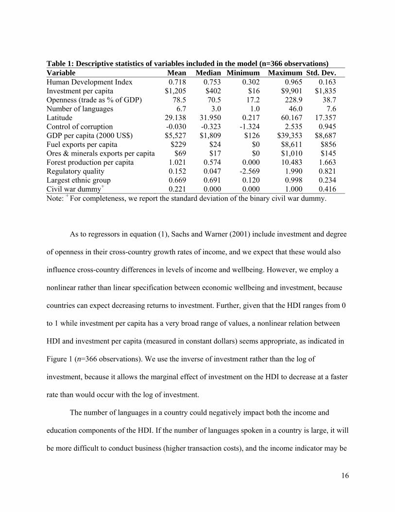
Table 1: Descriptive statistics of variables included in the model (n=366 observations) Variable Mean Median Minimum Maximum Std. Dev. Human Development Index 0.718 0.753 0.302 0.965 0.163 Investment per capita $1,205 $402 $16 $9,901 $1,835 Openness (trade as % of GDP) 78.5 70.5 17.2 228.9 38.7 Number of languages 6.7 3.0 1.0 46.0 7.6 Latitude 29.138 31.950 0.217 60.167 17.357 Control of corruption -0.030 -0.323 -1.324 2.535 0.945 GDP per capita (2000 US$) $5,527 $1,809 $126 $39,353 $8,687 Fuel exports per capita $229 $24 $0 $8,611 $856 Ores & minerals exports per capita $69 $17 $0 $1,010 $145 Forest production per capita 1.021 0.574 0.000 10.483 1.663 Regulatory quality 0.152 0.047 -2.569 1.990 0.821 Largest ethnic group 0.669 0.691 0.120 0.998 0.234 Civil war dummy+ 0.221 0.000 0.000 1.000 0.416 Note: + For completeness, we report the standard deviation of the binary civil war dummy.
As to regressors in equation (1), Sachs and Warner (2001) include investment and degree
of openness in their cross-country growth rates of income, and we expect that these would also
influence cross-country differences in levels of income and wellbeing. However, we employ a
nonlinear rather than linear specification between economic wellbeing and investment, because
countries can expect decreasing returns to investment. Further, given that the HDI ranges from 0
to 1 while investment per capita has a very broad range of values, a nonlinear relation between
HDI and investment per capita (measured in constant dollars) seems appropriate, as indicated in
Figure 1 (n=366 observations). We use the inverse of investment rather than the log of
investment, because it allows the marginal effect of investment on the HDI to decrease at a faster
rate than would occur with the log of investment.
The number of languages in a country could negatively impact both the income and
education components of the HDI. If the number of languages spoken in a country is large, it will
be more difficult to conduct business (higher transaction costs), and the income indicator may be

17
adversely affected. In addition, greater diversity of languages makes it more difficult for
governments to deliver educational services, and the education indicators may also be affected.
0.2
0.3
0.4
0.5
0.6
0.7
0.8
0.9
1.0
0 2,000 4,000 6,000 8,000 10,000
INVESTMENT_PC
HD
I
Investment per capita
Hum
an D
evel
opm
ent I
ndex
0.2
0.3
0.4
0.5
0.6
0.7
0.8
0.9
1.0
0 2,000 4,000 6,000 8,000 10,000
INVESTMENT_PC
HD
I
Investment per capita
Hum
an D
evel
opm
ent I
ndex
Figure 1: The Human Development Index vs. Investment Per Capita
Latitude is included in the HDI equation to capture other unobservable cross-country
differences, such as geography and climate, which may affect the overall standard of living. It
may also be a strong indicator of other important but otherwise unobservable differences across
countries. Theil and Chen (1995), and Theil and Galvez (1995), show that differences in latitude
can explain up to 70% of the variation in cross-country levels of income. Brunnshweiler and
Bulte (2007) use latitude as an instrument for institutional quality in their estimation of the
resource curse. In our data, the relationship between latitude and overall standards of living is
quite clear as indicated in Figure 2 (n=366); the correlation between the HDI and latitude is 0.61.
Countries farther from the equator (whether north or south) tend to have higher overall standards
of living, while those near the equator have lower overall standards of living.

18
0.2
0.3
0.4
0.5
0.6
0.7
0.8
0.9
1.0
0 10 20 30 40 50 60 70
LATITUDE
HD
IH
uman
Dev
elop
men
t Ind
ex
Near Equator Latitude Far From Equator
0.2
0.3
0.4
0.5
0.6
0.7
0.8
0.9
1.0
0 10 20 30 40 50 60 70
LATITUDE
HD
IH
uman
Dev
elop
men
t Ind
ex
Near Equator Latitude Far From Equator
Figure 2: Human Development Index vs. Latitude
Finally, control of corruption is included in equation (1) because, as discussed above, it is
through rent seeking and corruption that natural resources may lower overall levels of wellbeing.
The relationship between the control of corruption variable and the HDI is shown in Figure 3
(n=366). It appears that the data support the hypothesis that higher levels of corruption are
associated with lower levels of wellbeing. This general finding holds if we consider simple linear
or nonlinear relationships between the HDI and control of corruption.
In the control of corruption equation (2), exports and production of resources per capita
are used as proxies for resource rents. Potential rents from fuel resources and ores and mineral
resources are measured in terms of dollar exports per capita, while those from forest resources
are measured by the per capita volume of forestry production. In order to interpret the resulting
coefficients on resource rents appropriately, per capita GDP is included in the regression. If per
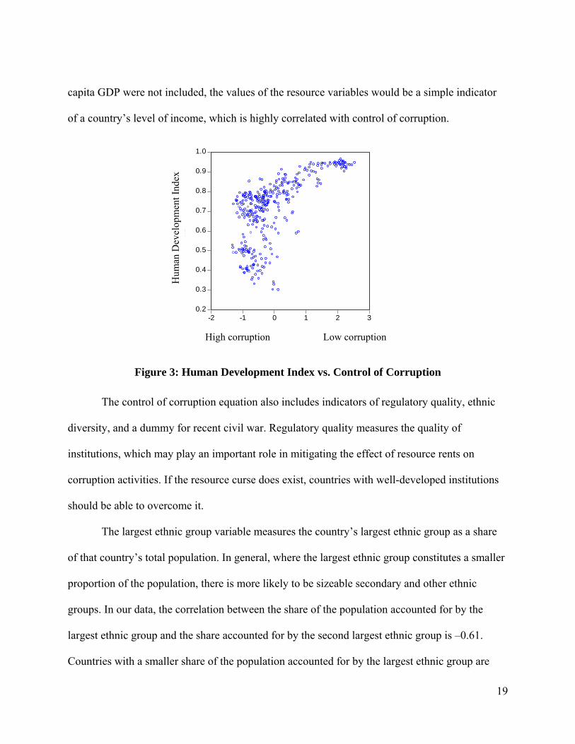
19
capita GDP were not included, the values of the resource variables would be a simple indicator
of a country’s level of income, which is highly correlated with control of corruption.
0.2
0.3
0.4
0.5
0.6
0.7
0.8
0.9
1.0
-2 -1 0 1 2 3
CONTROL_CORRUPTION
HD
IH
uman
Dev
elop
men
t Ind
ex
High corruption Low corruption
0.2
0.3
0.4
0.5
0.6
0.7
0.8
0.9
1.0
-2 -1 0 1 2 3
CONTROL_CORRUPTION
HD
IH
uman
Dev
elop
men
t Ind
ex
High corruption Low corruption
Figure 3: Human Development Index vs. Control of Corruption
The control of corruption equation also includes indicators of regulatory quality, ethnic
diversity, and a dummy for recent civil war. Regulatory quality measures the quality of
institutions, which may play an important role in mitigating the effect of resource rents on
corruption activities. If the resource curse does exist, countries with well-developed institutions
should be able to overcome it.
The largest ethnic group variable measures the country’s largest ethnic group as a share
of that country’s total population. In general, where the largest ethnic group constitutes a smaller
proportion of the population, there is more likely to be sizeable secondary and other ethnic
groups. In our data, the correlation between the share of the population accounted for by the
largest ethnic group and the share accounted for by the second largest ethnic group is –0.61.
Countries with a smaller share of the population accounted for by the largest ethnic group are

20
more likely to have secondary or tertiary ethnic groups of considerable size, which may lead to
ethnic tensions. These in turn may be associated with a greater risk of internal conflict, and hence
increased rent seeking. Internal conflict can lead to rent seeking and corruption as different
groups try to achieve political and economic power. Further, if there is civil war, looting of
natural resources may be more prevalent, increasing opportunities for bribery and corruption.
5. Empirical Results
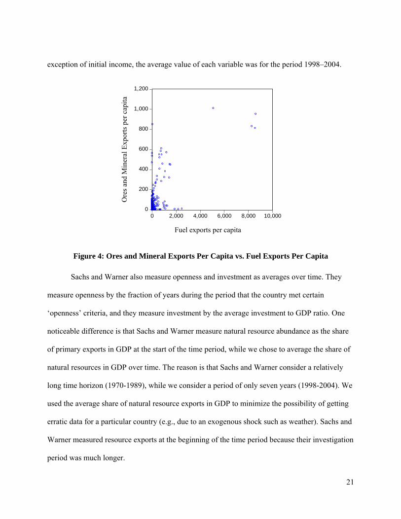
The dollar value of fuel exports per capita is plotted against the dollar value of ores and
mineral exports per capita in Figure 4. There are four clear points in the figure that are strong
outliers, with very high levels of natural resource exports per capita. The four outliers are for
Norway, thus providing evidence against the resource curse since Norway has a high HDI.
Including this country might bias the results in favour of rejecting the resource curse claim. Upon
estimating the model with and without this outlier, we found little impact on the results,
indicating that our conclusions would not be sensitive to the inclusion of Norway. Given there is
no reason to doubt the quality of data for this country, we chose to keep observations for Norway
in the analysis.
As a validity test and before estimating our model, we decided to find out how well our
data replicate those of Sachs and Warner (1995, Equation 1.4, Table 1, p.24). The dependent
variable we use in this case is the growth rate of real GDP per capita between 1998 and 2004.
Following Sachs and Warner (1995), we included estimates of initial income, investment,
openness and rule of law. Investment, openness and rule of law were measured in the same
manner as in our core model. The share of natural resource exports in GDP was derived from the
shares of agricultural, fuel, and ores and mineral exports in total merchandise exports. With the
21
exception of initial income, the average value of each variable was for the period 1998–2004.
0
200
400
600
800
1,000
1,200
0 2,000 4,000 6,000 8,000 10,000
FUEL_100
OR
ES_1
00O
res a
nd M
iner
al E
xpor
ts p
er c
apita
Fuel exports per capita
0
200
400
600
800
1,000
1,200
0 2,000 4,000 6,000 8,000 10,000
FUEL_100
OR
ES_1
00O
res a
nd M
iner
al E
xpor
ts p
er c
apita
Fuel exports per capita
Figure 4: Ores and Mineral Exports Per Capita vs. Fuel Exports Per Capita
Sachs and Warner also measure openness and investment as averages over time. They
measure openness by the fraction of years during the period that the country met certain
‘openness’ criteria, and they measure investment by the average investment to GDP ratio. One
noticeable difference is that Sachs and Warner measure natural resource abundance as the share
of primary exports in GDP at the start of the time period, while we chose to average the share of
natural resources in GDP over time. The reason is that Sachs and Warner consider a relatively
long time horizon (1970-1989), while we consider a period of only seven years (1998-2004). We
used the average share of natural resource exports in GDP to minimize the possibility of getting
erratic data for a particular country (e.g., due to an exogenous shock such as weather). Sachs and
Warner measured resource exports at the beginning of the time period because their investigation
period was much longer.

22
Sachs and Warner (1995) include 62 countries, but they do not provide a list of which
ones, although they (1997b) do discuss a number of African countries that are missing from their
analysis and make reasonable predictions of growth for those missing countries. With the
exception of Mauritius and Togo, the same countries are missing from our data as well. As
discussed in Appendix B, our data include 88 countries that represent a wide range of economies.
Consistent with Sachs and Warner, we do not allow for individual country effects. The
estimation results are provided in Table 2.2 They confirm our prior expectations: Consistent with
economic theory, the signs on initial income and the inverse of investment are negative, while
those on openness and rule of law are positive, and all are statistically significant. Note that we
are unable to reproduce Sachs and Warner’s finding regarding the natural resource curse – the
coefficient on natural resource dependence is insignificant. For comparison, Sachs and Warner’s
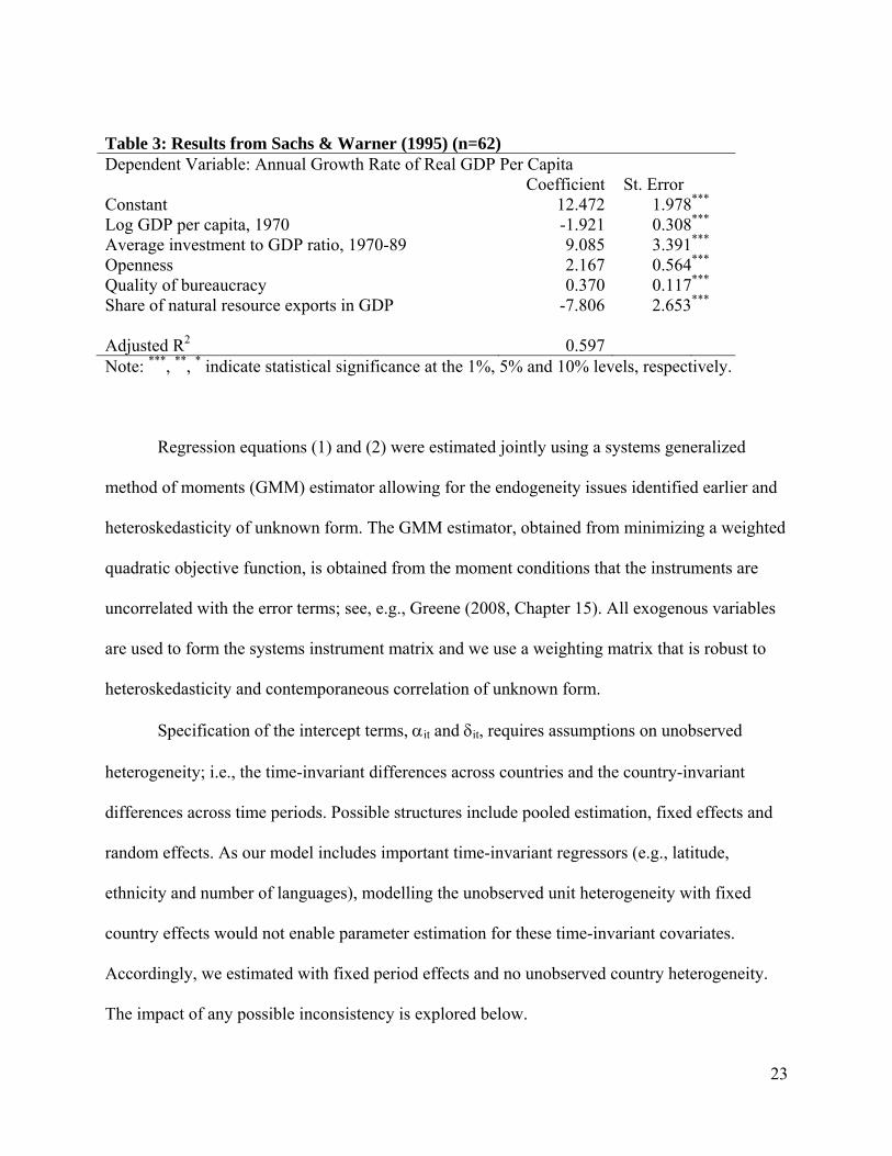
(1995) results are provided in Table 3. Their general conclusion regarding the resource curse
does not appear to be robust. We investigate this further using our two-equation model.
Table 2: OLS estimation using a traditional model of the resource curse (n=88) Dependent Variable: Growth Rate of Real GDP Per Capita, 1998-2004 Coefficient St. Error Constant 110.818 23.115***
Log GDP per capita, 1998 -12.173 2.761***
Inverse of investment per capita -1383.082 381.682***
Openness 0.090 0.027***
Rule of law 9.368 3.228***
Share of natural resource exports in GDP 0.051 0.231 Adjusted R2 0.208 Note: Estimated standard errors are heteroskedasticity consistent. ***, **, * indicate statistical significance at the 1%, 5% and 10% levels, respectively.
2 All estimation is undertaken using EViews 6.
23
Table 3: Results from Sachs & Warner (1995) (n=62) Dependent Variable: Annual Growth Rate of Real GDP Per Capita Coefficient St. Error Constant 12.472 1.978***
Log GDP per capita, 1970 -1.921 0.308***
Average investment to GDP ratio, 1970-89 9.085 3.391***
Openness 2.167 0.564***
Quality of bureaucracy 0.370 0.117***
Share of natural resource exports in GDP -7.806 2.653***
Adjusted R2 0.597 Note: ***, **, * indicate statistical significance at the 1%, 5% and 10% levels, respectively.
Regression equations (1) and (2) were estimated jointly using a systems generalized
method of moments (GMM) estimator allowing for the endogeneity issues identified earlier and
heteroskedasticity of unknown form. The GMM estimator, obtained from minimizing a weighted
quadratic objective function, is obtained from the moment conditions that the instruments are
uncorrelated with the error terms; see, e.g., Greene (2008, Chapter 15). All exogenous variables
are used to form the systems instrument matrix and we use a weighting matrix that is robust to
heteroskedasticity and contemporaneous correlation of unknown form.
Specification of the intercept terms, αit and δit, requires assumptions on unobserved
heterogeneity; i.e., the time-invariant differences across countries and the country-invariant
differences across time periods. Possible structures include pooled estimation, fixed effects and
random effects. As our model includes important time-invariant regressors (e.g., latitude,
ethnicity and number of languages), modelling the unobserved unit heterogeneity with fixed
country effects would not enable parameter estimation for these time-invariant covariates.
Accordingly, we estimated with fixed period effects and no unobserved country heterogeneity.
The impact of any possible inconsistency is explored below.
24
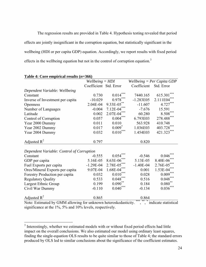
The regression results are provided in Table 4. Hypothesis testing revealed that period
effects are jointly insignificant in the corruption equation, but statistically significant in the
wellbeing (HDI or per capita GDP) equation. Accordingly, we report results with fixed period
effects in the wellbeing equation but not in the control of corruption equation.3
Table 4: Core empirical results (n=366) Wellbeing = HDI Wellbeing = Per Capita GDP Coefficient Std. Error Coefficient Std. Error Dependent Variable: Wellbeing Constant 0.730 0.014*** 7440.165 615.301***
Inverse of Investment per capita -10.029 0.978*** -1.283E05 2.111E04***
Openness 2.04E-04 9.33E-05** -11.607 4.727***
Number of Languages -0.004 7.12E-04*** -7.676 15.591Latitude 0.002 2.07E-04*** 60.280 8.508***
Control of Corruption 0.057 0.004*** 6.793E03 278.488***
Year 2000 Dummy 0.011 0.010 563.928 410.748Year 2002 Dummy 0.017 0.009* 1.036E03 403.728***
Year 2004 Dummy 0.032 0.010*** 1.454E03 421.323***
Adjusted R2 0.797 0.820 Dependent Variable: Control of Corruption Constant -0.555 0.054*** -0.546 0.046***
GDP per capita 5.16E-05 8.63E-06*** 5.13E-05 8.40E-06***
Fuel Exports per capita -1.29E-04 2.78E-05*** -1.40E-04 2.76E-05***
Ores/Mineral Exports per capita 9.07E-04 1.68E-04*** 0.001 1.53E-04***
Forestry Production per capita 0.032 0.010*** 0.028 0.009***
Regulatory Quality 0.533 0.048*** 0.516 0.048***
Largest Ethnic Group 0.199 0.090** 0.184 0.080**
Civil War Dummy -0.110 0.040*** -0.134 0.036***
Adjusted R2 0.865 0.864 Note: Estimated by GMM allowing for unknown heteroskedasticity. ***, **, * indicate statistical significance at the 1%, 5% and 10% levels, respectively.
3 Interestingly, whether we estimated models with or without fixed period effects had little impact on the overall conclusions. We also estimated our model using ordinary least squares, finding the single-equation OLS results to be quite similar to those of Table 4; the standard errors produced by OLS led to similar conclusions about the significance of the coefficient estimates.
25
Discussion
We first examine the results with wellbeing measured by the HDI index. As expected, the
sign on the inverse of investment per capita in the HDI equation was negative, suggesting that
higher levels of investment are associated with higher levels of the HDI. This result is
statistically significant at the 99% confidence level. The coefficient on the openness variable also
has the expected sign (positive), indicating that more open countries have higher standards of
living, which accords with Sachs and Warner’s model of economic growth. However, sensitivity
analysis (not reported here but available upon request) indicates that the sign and statistical
significance of the openness variable is not robust to econometric methodology.
The sign on the number of languages coefficient was negative, confirming the
expectation that an increase in number of languages is associated with decreased levels of
income and education. An increase in the number of languages in a given country should make it
more difficult to conduct economic transactions and deliver educational services, thereby
decreasing income, literacy rates and educational enrolment. Together these three indicators
form two-thirds of the Human Development Index.
The coefficient on latitude was positive and significant, implying that countries farther
away from the equator tend to have higher standards of living. Control of corruption was
positively associated with the HDI, suggesting that countries with more corruption tend to have
lower levels of wellbeing. This finding confirms the first part of the transmission mechanism
through which we expect the resource curse (if it exists) to operate.
In comparison to the HDI results, when the dependent variable is PPP-adjusted GDP per
capita the openness variable has an unexpected sign and the number of languages variable is no
longer significant. In the control of corruption equation, the coefficients on each of the resource

26
rent variables are significant, although the signs vary. The coefficients on ores and mineral
exports and forestry production per capita are positive, while the coefficient on fuel exports is
negative. Regulatory quality is positively associated with control over corruption, and the result
is significant, indicating that, even if resources are a curse, improved institutional quality can
help overcome this obstacle. Countries with better institutions tend to have more control over
corruption and rent seeking. Finally, countries with a larger share of their population accounted
for by the largest ethnic group (less ethnic diversity) experienced less corruption, and countries
that experienced civil war experienced more corruption. These findings confirm our hypothesis
that increased ethnic diversity and civil war provide opportunities for rent seeking and corruption
as different groups try to gain political power. Overall, however, our finding that rents from fuel
resources are an important part of the resource curse continues to hold.
To determine the relative importance of our explanatory variables with HDI as the
measure of standard of living, we report standardized regression coefficients (beta coefficients)
in Table 5. Such coefficients are also used by Bulte, Damania and Deacon (2005), for example.
We computed beta coefficients for each of the variables of interest by multiplying each
coefficient estimate from the core model (Table 4) by each variable’s standard deviation (Table
1), and then dividing by the standard deviation of the associated dependent variable.4 The
reported beta coefficients measure the magnitude of each variable in terms of standard
deviations, providing one way of ascertaining the relative contribution of the variable to the
prediction of the dependent variable. For example, a one standard deviation increase in numbers
of languages variable is associated with a 0.21 standard deviations decrease in the HDI, ceteris
4 The standard deviation of the inverse of investment per capita is not provided in Table 1. This standard deviation was computed separately as equal to 8.164E-03.

27
paribus. From the table, investment and control of corruption are the two most important
indicators of a country’s standard of living, while openness appears to be less important.
Table 5: Standardized regression coefficients (beta coefficients) from the core model
Human Development Index beta
coefficient
Control of Corruption beta
coefficient Inverse of Investment per capita -0.50 GDP per capita 0.47Openness 0.05 Fuel Exports per capita -0.12Number of Languages -0.21 Ores/Mineral Exports per capita 0.14Latitude 0.16 Forestry Production per capita 0.06Control of Corruption 0.33 Regulatory Quality 0.46 Largest Ethnic Group 0.05 Civil War Dummy+ -0.05Note: +Although it is meaningless to consider the standard deviation of a dummy variable, we report the civil war dummy variable’s beta coefficient for completeness.
In the control of corruption equation, per capita GDP and regulatory quality appear to be
the most important indicators of the dependent variable. Although the coefficients on resource
exports per capita are smaller, they all appear to contribute more to the prediction of control of
corruption than the ethnicity and civil war variables. The beta coefficient on fuel exports per
capita is -0.14, and the beta coefficient on ores and mineral exports per capita is 0.15. Bulte,
Damania and Deacon (2005) estimated the impact of point resources (resources concentrated in a
narrow geographic region, including oil, minerals, and plantations) on two measures of
institutional quality: rule of law and government effectiveness. In the rule of law equation, they
obtained a beta coefficient of -0.21 on point resources, and in the government effectiveness
equation, they obtained a beta coefficient of -0.27 on point resources. In comparison, the beta
coefficients we obtain on fuel exports and ores and mineral exports seem reasonable.
The results suggest that in determining whether or not natural resources are a curse or a
blessing, individual types of natural resources must be considered separately. If all types of
28
resources are aggregated into one measure, the positive and negative impacts of different
resource types would offset each other, resulting in insignificant results and misleading
conclusions. Our results suggest that fuel resources can be considered a curse, because large
rents available from exploitation of fuel resources are associated with increased levels of rent
seeking and corruption that lead, in turn, to lower standards of living. A similar conclusion was
reached by Fearon (2005), who demonstrates that oil exports are positively associated with
increased risk of internal conflict. In our analyses, institutional quality can offset the impact of
the fuel resource curse. As indicated in Table 5, the magnitude of the regulatory quality variable
is much greater than that of the fuel exports per capita variable. This suggests that improvements
in institutional quality can more than offset the curse of fuel resources. This might explain why
some countries, such as Norway, have both high levels of fuel exports per capita and high
standards of living. On the other hand, availability of ores and minerals, and to a lesser extent
forest resources, might be a blessing rather than a curse.
Sensitivity Analysis
OLS is used to estimate each of the model equations separately, using a pooled estimator
and, to allow for individual country unobserved heterogeneity, by fixed-effects and random-
effects estimation. For the fixed effects case, we had to drop the time-invariant variables.
Regression results are provided in Table 6. In each case, we continue to allow for period fixed
effects in the HDI equation but not in the control of corruption equation. We observe that the
pooled estimates using the independent equations are quite similar to those obtained with our
systems GMM estimator (Table 4), although the latter is more appropriate because it explicitly
allows for endogeneity of some of the regressors.

29
Table 6: Estimation of the system using separate equations Pooled Fixed effects Random effects Coefficient Std. Error Coefficient Std. Error Coefficient Std. ErrorHuman Development Index Constant 0.728 0.015 *** 0.693 0.008 *** 0.658 0.019 ***
Inverse of Investment per capita -9.277 0.570 *** -0.158 0.468 -1.890 0.425 ***
Openness 1.47E-04 1.02E-04 * 1.14E-04 9.04E-05 8.84E-05 8.08E-05Number of Languages -0.005 0.001 *** n/i n/i -0.008 0.001 ***
Latitude 0.002 2.72E-04 *** n/i n/i 0.003 4.46E-04 ***
Control of Corruption 0.053 0.005 *** 0.015 0.006 *** 0.030 0.005 ***
Year 2000 Dummy 0.009 0.011 0.019 0.002 *** 0.019 0.002 ***
Year 2002 Dummy 0.014 0.011 0.020 0.002 *** 0.020 0.002 ***
Year 2004 Dummy 0.029 0.011 *** 0.033 0.002 *** 0.032 0.002 ***
Adjusted R2 0.797 0.995 0.602
Control of Corruption Constant -0.571 0.058 *** -0.129 0.085 * -0.673 0.100 ***
GDP per capita 4.49E-05 3.32E-06 *** 1.30E-05 1.71E-05 6.08E-05 5.25E-06 ***
Fuel Exports per capita -1.17E-06 2.95E-07 *** -8.37E-07 4.41E-07 ** -1.02E-06 3.06E-07 ***
Ores/Mineral Exports per capita 1.14E-05 1.99E-06 *** -3.51E-06 3.07E-06 4.32E-06 2.13E-06 **
Forestry Production per capita 0.042 0.012 *** 0.050 0.034 * 0.069 0.019 ***
Regulatory Quality 0.520 0.034 *** 0.139 0.035 *** 0.240 0.031 ***
Largest Ethnic Group 0.209 0.082 *** n/i n/i 0.341 0.145 ***
Civil War Dummy -0.110 0.045 *** n/i n/i -0.189 0.080 ***
Adjusted R2 0.868 0.982 0.607
Note: n/i = not included as these are time-invariant regressors. ***, **, * indicate statistical significance at the 1%, 5% and 10% levels, respectively.

30
Many of the qualitative conclusions from the model are the same regardless of which
estimator is employed. One notable exception is the effect of ores and mineral resources on
control of corruption. In the pooled and random-effects models, this variable has a significant
positive impact on control of corruption, but is insignificant in the fixed-effects model.
The estimates reported in Table 6 provide a means of examining whether there is
unmodelled country specific heterogeneity. In the core model, the time-invariant variables
(latitude, number of languages, ethnicity and civil war dummy) allow for some country specific
differences but other unobserved heterogeneity may remain. Because these time-invariant
variables are dropped from the fixed-effects equations, the resulting country specific constant
terms (not reported in Table 6) capture the differences across countries from these observable
variables included in the core model and any other relevant unspecified time-invariant
covariates. To test for unobserved heterogeneity, we compare the sum of squared residuals from
each pooled equation to those from each fixed-effects equation using an F-test. Results in Table
7 clearly indicate that further (unobserved) country-specific heterogeneity exists.
We also compare the fixed-effects and random-effects estimates using a Hausmann
(1978) test. The outcome supports the use of fixed effects over random effects, and it implies that
the unobserved heterogeneous effects are correlated with other variables in the model, so that the
pooled estimator is also likely inconsistent.
31
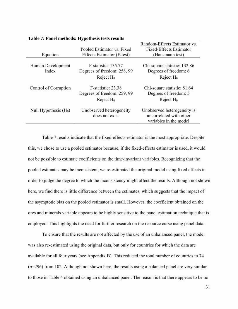
Table 7: Panel methods: Hypothesis tests results
Equation Pooled Estimator vs. Fixed Effects Estimator (F-test)
Random-Effects Estimator vs. Fixed-Effects Estimator
(Hausmann test) Human Development F-statistic: 135.77 Chi-square statistic: 132.86
Index Degrees of freedom: 258, 99 Degrees of freedom: 6 Reject H0 Reject H0
Control of Corruption F-statistic: 23.38 Chi-square statistic: 81.64 Degrees of freedom: 259, 99 Degrees of freedom: 5 Reject H0 Reject H0
Null Hypothesis (H0) Unobserved heterogeneity does not exist
Unobserved heterogeneity is uncorrelated with other variables in the model
Table 7 results indicate that the fixed-effects estimator is the most appropriate. Despite
this, we chose to use a pooled estimator because, if the fixed-effects estimator is used, it would
not be possible to estimate coefficients on the time-invariant variables. Recognizing that the
pooled estimates may be inconsistent, we re-estimated the original model using fixed effects in
order to judge the degree to which the inconsistency might affect the results. Although not shown
here, we find there is little difference between the estimates, which suggests that the impact of
the asymptotic bias on the pooled estimator is small. However, the coefficient obtained on the
ores and minerals variable appears to be highly sensitive to the panel estimation technique that is
employed. This highlights the need for further research on the resource curse using panel data.
To ensure that the results are not affected by the use of an unbalanced panel, the model
was also re-estimated using the original data, but only for countries for which the data are
available for all four years (see Appendix B). This reduced the total number of countries to 74
(n=296) from 102. Although not shown here, the results using a balanced panel are very similar
to those in Table 4 obtained using an unbalanced panel. The reason is that there appears to be no
32
systematic bias in dropping observations as both developed countries (e.g., Canada and Belgium)
and developing countries (e.g., Cambodia and Ecuador) are dropped. The coefficient on the
openness variable doubled, but all other coefficient estimates were remarkably similar. The
coefficient on largest ethnic group was no longer significant, but this could be a direct result of
the decrease in the available number of observations. Thus, we continue to rely on the results in
Table 4, because, as Baltagi and Chang (2000) show, using an unbalanced panel is preferable to
dropping observations just to balance the panel.
To determine how sensitive the results are to the specification of resource abundance, the
core model was also re-estimated using the more conventional measure of resource abundance,
the share of natural resource exports in GDP. In this case, the coefficient on resource abundance
in the corruption equation is negative (-0.001), suggesting that resource abundance is indeed a
curse, but the estimate is statistically insignificant (standard error = 0.002). This again highlights
the need to specify an appropriate transmission mechanism between resources and wellbeing,
and the importance of providing an appropriate measure of natural resource abundance.
7. Concluding Remarks
We evaluated the natural resource curse by considering the potential for resource rents to
lead to corruption and rent seeking, which in turn affect standards of living or wellbeing. This is
in contrast to traditional models of the natural resource curse that have focussed on using the
share of primary product exports in GDP to explain differences in growth rates of GDP across
countries. We also measured resource abundance in per capita terms, rather than as the relative
share of resources in GDP. Finally, we examined the effect of natural resource abundance on the
overall standard of living as measured by the Human Development Index rather than GDP,

33
although results for PPP-adjusted per capita GDP are similar to those using the HDI.
Our findings indicate that it is important to treat different types of natural resources
separately when addressing the validity of the resource curse hypothesis. Fuel resources are
associated with increased rent seeking and potential corruption, suggesting that fuel resources
may be considered a ‘curse’. Forest resources on the other hand appear to be associated with
decreased rent seeking and corruption, indicating that forest resources may be a blessing rather
than a curse. However, we did not distinguish between pristine and plantation forests, with the
former capable of generating much greater rents than the latter. The relationship between ores
and mineral resources appears to be positive, also suggesting that these resources are a blessing,
although this result is sensitive to panel data estimation techniques and warrants further
investigation. Through their impact on rent seeking and corruption, rents from fuel resources
negatively impact overall standards of living across countries, as measured by both HDI and per
capita GDP. This effect can be mitigated, however, by improving institutional quality in many
countries so that rent seeking is minimized.
While our research focussed on a relatively short time horizon, it would be interesting to
study how natural resource abundance impacts long-term changes in countries’ standards of
living as more data become available. This could be done by using panel data that span a longer
time horizon with longer intervals between periods.
Finally, natural resources provide a valuable flow of income to various countries.
Throughout history, some resource-rich countries have grown rapidly and achieved high
standards of living, while others have experienced corruption, civil war and widespread poverty.
The relationship between natural resource abundance and overall standards of living is extremely
complicated, and, before making any general claim about whether or not natural resources are a

34
curse or a blessing, researchers should spend more time considering the mechanisms through
which resource rents may help or hinder economic development. If resource rents are invested in
infrastructure and social programs that increase long-term economic growth and distribute
wealth to those in need, resource rents have the potential to increase overall standards of living.
But if resource rents are captured by special interest groups and dissipated through corruption
and rent-seeking behavior, resource rents may lead to lower overall standards of living and
higher income inequality within countries. The capacity for resource rents to improve, rather
than inhibit, economic development depends in large part on the role of government institutions
and the nature of the resources generating the rents.
References
Ades, Alberto and Di Tella, Rafael. 1999. “Rents, Competition, and Corruption.” American Economic Review, 89(4), pp.982-993.
Anderson, T.L., and Hill, P.J. 2004. The Not So Wild, Wild West. Property Rights on the Frontier. Stanford University Press, Stanford, CA
Auty, Richard M. 1993. Sustaining Development in Mineral Economies: The Resource Curse Thesis. London and New York: Routledge.
Azfar, Omar, Young, Lee, and Swamy, Anand. 2001. “The Causes and Consequences of Corruption.” Annals of the American Academy of Political and Social Science, Vol. 573, Culture and Development: International Perspectives, pp.42-56.
Baltagi, Badi H., and Chang, Young-Jae. 2000. “Simultaneous Equations with Incomplete Panels.” Econometric Theory, 16(2), pp.269-279.
Barbier, Edward B. 2003. “The Role of Natural Resources in Economic Development.” Australian Economic Papers, 42(2), pp.253-272.
Brunnshweiler, Christa N., and Bulte, Erwin H. 2006. “The Resource Curse Revisited and Revised: A Tale of Paradoxes and Red Herrings.” Center of Economic Research at ETH Zurich Working Paper, No. 06/61, Zurich, Switzerland.
Bulte, Erwin H., Damania, Richard, and Deacon, Robert T. 2005. “Resource Intensity, Institutions, and Development.” World Development, 33(7), pp.1029-1044.
CIA (Central Intelligence Agency). 2007. The World Factbook. https://www.cia.gov/library/publications/the-world-factbook/index.html

35
Collier, Paul, and Goderis, Benedikt. 2007. “Commodity Prices, Growth, and the Natural Resource Curse: Reconciling a Conundrum.” CSAE Working Paper: CSAE WPS/2007-15. http://www.csae.ox.ac.uk/workingpapers/pdfs/2007-15text.pdf
Collier, Paul, and Hoeffler, Anke. 2004. “Greed and Grievance in Civil War.” Oxford Economic Papers, 56(4), pp.563-96.
. 2005. “Resource Rents, Governance, and Conflict.” Journal of Conflict Resolution, 49(4), pp.625-632.
De Soto, Hernando. 2000. The Mystery of Capital. Why Capitalism Triumphs in the West and Fails Everywhere Else. New York, NY: Basic Books.
de Soysa, Indra. 2002. “Paradise Is a Bazaar? Greed, Creed, and Governance in Civil War, 1989-99.” Journal of Peace Research, 39(4), pp.395-416.
Deaton, Angus. 1999. “Commodity Prices and Growth in Africa.” Journal of Economic Perspectives, 13(3), pp.23-40.
Fearon, James D. 2005. “Primary Commodity Exports and Civil War.” Journal of Conflict Resolution, 49(4), pp.483-507.
Fearon, James D. and Laitin, David D. 2003. “Ethnicity, Insurgency, and Civil War.” American Political Science Review, 97(1), pp.75-90.
Folmer, Henk and G. Cornelis van Kooten. 2007. “Deforestation.” Chapter 7 in Solutions for the World's Biggest Problems: Costs and Benefits edited by Bjorn Lomborg. Cambridge, UK: Cambridge University Press.
Gelb, Alan H. 1988. Oil Windfalls: Blessing or Curse? Oxford: Oxford University Press.
Greene, William H. 2008. Econometric Analysis, 6th Edition. Upper Saddle River, NJ: Pearson-Prentice Hall.
Gylfason, Thorvaldur. 2001. “Natural Resources and Economic Growth: What is the Connection?” Center for Economic Studies & Ifo Institute for Economic Research Working Paper, No. 530, Munich, Germany.
Gylfason, Thorvaldur. 2002. “Mother Earth: Ally or Adversary?” World Economics, 3(1), pp.7-24.
Hausmann, Jerry A. 1978. “Specification Tests in Econometrics.” Econometrica, 46(6), pp. 1251-1271.
Huntington, Samuel P. 1968. Political Order in Changing Societies. New Haven, CT: Yale University Press.
Kaufmann, Daniel, Kraay, Aart, and Mastruzzi, Massimo. 2007. “Governance Matters VI: Governance Indicators for 1996-2006.” World Bank Policy Research Working Paper, No. 4280. Data: http://info.worldbank.org/governance/wgi2007/
Kronenberg, Tobias. 2004. “The Curse of Natural Resources in the Transition Economies.” Economics of Transition, 12(3), pp.399-426.
36
Leff, Nathaniel. 1964. “Economic Development through Bureaucratic Corruption.” American Behavioral Scientist, 8(3), pp.8-14.
Lewis, W. Arthur. 1954. “Economic Development with Unlimited Supplies of Labour.” The Manchester School, 28(2), pp.139-191.
Lujala, Päivi, Gleditsch, Nils Petter, and Gilmore, Elisabeth. 2005. “A Diamond Curse?: Civil War and a Lootable Resource.” Journal of Conflict Resolution, 49(4), pp.538-562.
Manzano, Osmel and Rigobon, Roberto. 2001. “Resource Curse or Debt Overhang?” National Bureau of Economic Research Working Paper, No. 8390, Cambridge, MA.
Mauro, Paolo. 1995. “Corruption and Growth.” Quarterly Journal of Economics, 110(3), pp.681-712.
Montenegro, Alvaro. 2004. “An Economic Development Index.” Econ WPA Working Paper, Development and Comp Systems Series, No. 0404010. Available at: http://ideas.repec.org/p/wpa/wuwpdc/0404010.html
Murphy Kevin M., Shleifer, Andrei, and Vishny, Robert W. 1989. “Industrialization and the Big Push.” Journal of Political Economy, 97(5), pp.1003-1026.
Naidoo, Robin. 2004. “Economic Growth and Liquidation of Natural Capital: The Case of Forest Clearance.” Land Economics, 80(2), pp.194-208.
Papyrakis, Ellissaios and Gerlagh, Reyer. 2004. “The Resource Curse Hypothesis and its Transmission Channels.” Journal of Comparative Economics, 32(1), pp.181-193.
Sachs, Jeffrey D. and Warner, Andrew M. 1995. “Natural Resource Abundance and Economic Growth.” National Bureau of Economic Research Working Paper, No. 5398, Cambridge, MA.
. 1997a. “Natural Resource Abundance and Economic Growth .” Revised version. Unpublished manuscript. Harvard Institute for International Development, Cambridge, MA.
. 1997b. “Sources of Slow Growth in African Economies.” Journal of African Economies. 6(3), pp.335-376.
. 1999. “The Big Push, Natural Resource Booms and Growth.” Journal of Development Economies. 59(1), pp.43-76.
. 2001. “The Curse of Natural Resources.” European Economic Review, 45(4-6), pp.827-838.
Sala-i-Martin, Xavier. 1997. “I Just Ran Two Million Regressions.” American Economic Review, 87(2), pp.178-183.
Sala-i-Martin, Xavier, Doppelhofer, Gernot, and Miller, Ronald. 2003. “Determinants of Long-Term Growth: A Bayesian Averaging of Classical Estimates (BACE) Approach.” American Economic Review, 94(4), pp.813-835.
Sala-i-Martin, Xavier and Subramanian, Arvind. 2003. “Addressing the Natural Resource Curse: An Illustration from Nigeria.” National Bureau of Economic Research Working Paper, No. 9804, Cambridge, MA.
37
Theil, Henri and Chen, Dongling. 1995. “The Equatorial Grand Canyon.” De Economist, 143(3), pp.317-327.
Theil, Henri and Galvez, Janet. 1995. “On Latitude and Affluence: The Equatorial Grand Canyon.” Empirical Economics, 20(1), pp.163-166.
Todaro, Michael P., and Smith, Stephen C. 2002. Economic Development. Eight Ed. New York: Addison-Wesley.
UNCDB (United Nations Common Database). 2007. http://unstats.un.org/unsd/cdb/cdb_help/cdb_quick_start.asp
UNDP (United Nations Development Programme). 2000, 2002, 2004, & 2006. Human Development Reports, selected years. Available at: http://hdr.undp.org/en/reports/
van Kooten, G. Cornelis and Folmer, Henk. 2004. Land and Forest Economics. Cheltenham, UK: Edward Elgar.
Weil, David N. 2005. Economic Growth. Boston, MA: Addison-Wesley.
World Bank. 2007. World Development Indicators 2007. http://www.worldbank.org/ .

38
Appendix A: Data Definitions
Human Development Index
Weighted index comprised of GDP per capita (purchasing power parity), adult life
expectancy at birth, adult literacy rate, and combined gross school enrolment rate
Source: United Nations Human Development Reports, selected years
Investment per capita
Gross capital formation (constant 2000 US$) per capita
Source: World Bank Development Indicators
Openness
Trade volume expressed as a percentage of GDP
Source: World Bank Development Indicators
Number of Languages
Number of languages in Ethnologue that exceed minimum threshold (1% of population or
1 million speakers)
Country observations are time invariant
Data available at: http://www.stanford.edu/~jfearon/
Source: Fearon and Laitin (2003)
Control of Corruption
Measures the extent to which public power is exercised for private gain, including both
petty and grand forms of corruption, as well as “capture” of the state by elites and private
interest
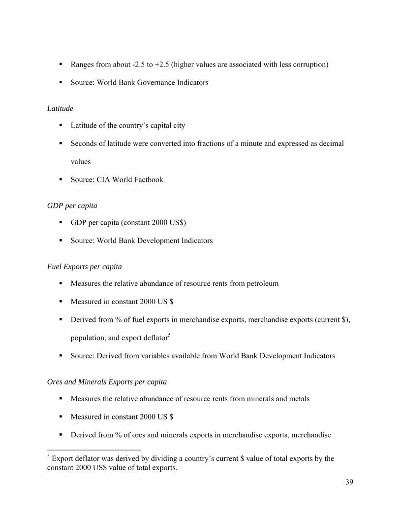
39
Ranges from about -2.5 to +2.5 (higher values are associated with less corruption)
Source: World Bank Governance Indicators
Latitude
Latitude of the country’s capital city
Seconds of latitude were converted into fractions of a minute and expressed as decimal
values
Source: CIA World Factbook
GDP per capita
GDP per capita (constant 2000 US$)
Source: World Bank Development Indicators
Fuel Exports per capita
Measures the relative abundance of resource rents from petroleum
Measured in constant 2000 US $
Derived from % of fuel exports in merchandise exports, merchandise exports (current $),
population, and export deflator5
Source: Derived from variables available from World Bank Development Indicators
Ores and Minerals Exports per capita
Measures the relative abundance of resource rents from minerals and metals
Measured in constant 2000 US $
Derived from % of ores and minerals exports in merchandise exports, merchandise
5 Export deflator was derived by dividing a country’s current $ value of total exports by the constant 2000 US$ value of total exports.
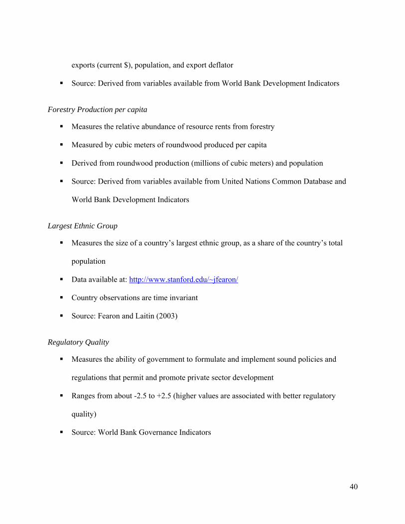
40
exports (current $), population, and export deflator
Source: Derived from variables available from World Bank Development Indicators
Forestry Production per capita
Measures the relative abundance of resource rents from forestry
Measured by cubic meters of roundwood produced per capita
Derived from roundwood production (millions of cubic meters) and population
Source: Derived from variables available from United Nations Common Database and
World Bank Development Indicators
Largest Ethnic Group
Measures the size of a country’s largest ethnic group, as a share of the country’s total
population
Data available at: http://www.stanford.edu/~jfearon/
Country observations are time invariant
Source: Fearon and Laitin (2003)
Regulatory Quality
Measures the ability of government to formulate and implement sound policies and
regulations that permit and promote private sector development
Ranges from about -2.5 to +2.5 (higher values are associated with better regulatory
quality)
Source: World Bank Governance Indicators
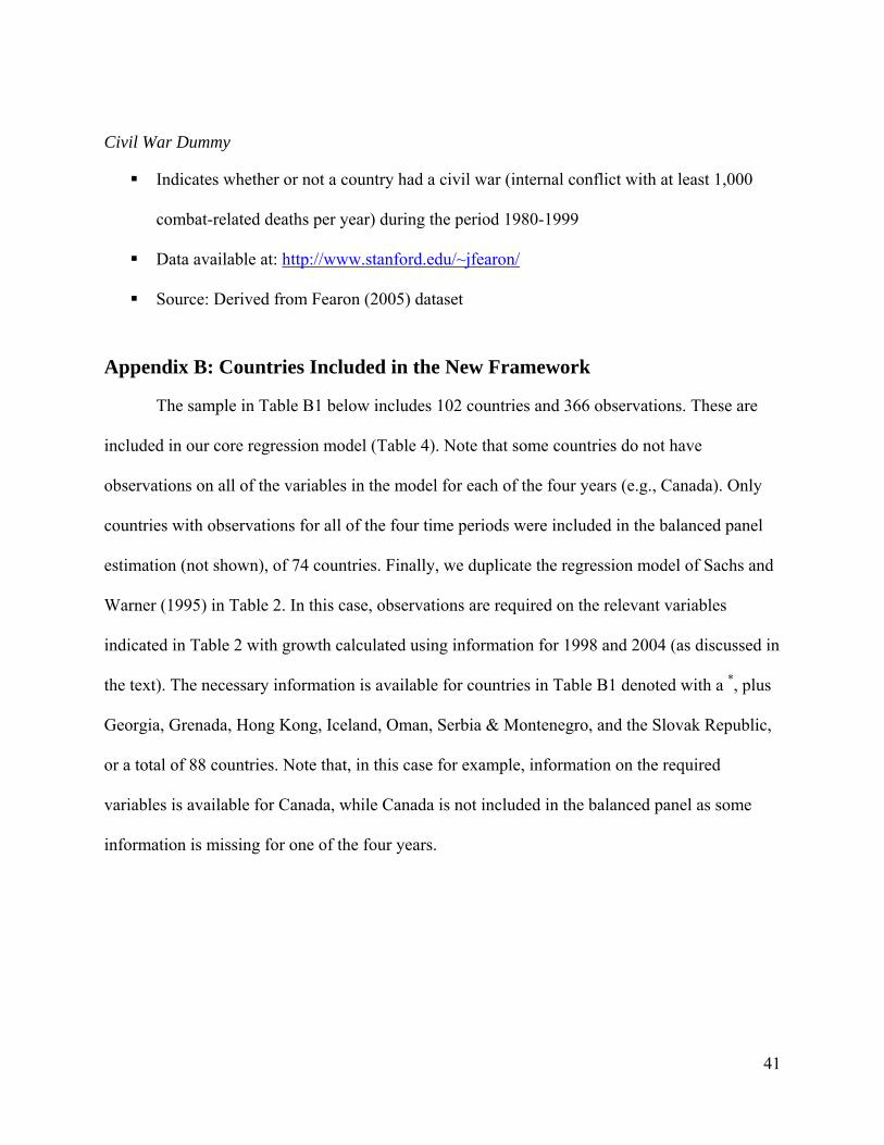
41
Civil War Dummy
Indicates whether or not a country had a civil war (internal conflict with at least 1,000
combat-related deaths per year) during the period 1980-1999
Data available at: http://www.stanford.edu/~jfearon/
Source: Derived from Fearon (2005) dataset
Appendix B: Countries Included in the New Framework
The sample in Table B1 below includes 102 countries and 366 observations. These are
included in our core regression model (Table 4). Note that some countries do not have
observations on all of the variables in the model for each of the four years (e.g., Canada). Only
countries with observations for all of the four time periods were included in the balanced panel
estimation (not shown), of 74 countries. Finally, we duplicate the regression model of Sachs and
Warner (1995) in Table 2. In this case, observations are required on the relevant variables
indicated in Table 2 with growth calculated using information for 1998 and 2004 (as discussed in
the text). The necessary information is available for countries in Table B1 denoted with a *, plus
Georgia, Grenada, Hong Kong, Iceland, Oman, Serbia & Montenegro, and the Slovak Republic,
or a total of 88 countries. Note that, in this case for example, information on the required
variables is available for Canada, while Canada is not included in the balanced panel as some
information is missing for one of the four years.
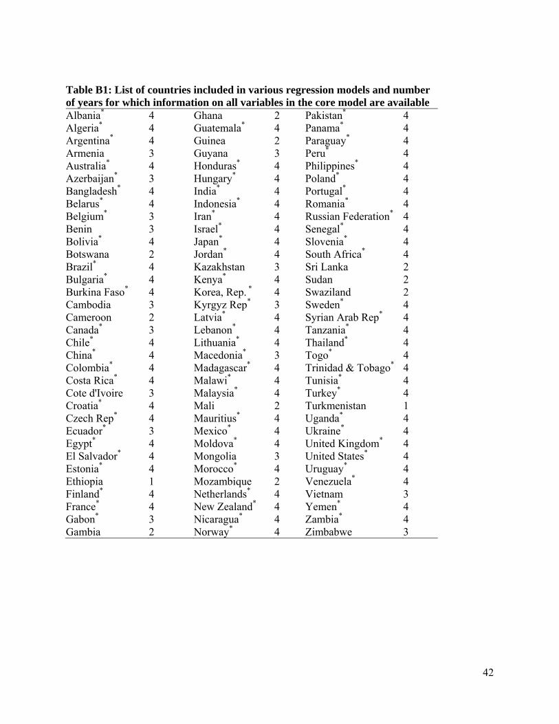
42
Table B1: List of countries included in various regression models and number of years for which information on all variables in the core model are available Albania* 4 Ghana 2 Pakistan* 4 Algeria* 4 Guatemala* 4 Panama* 4 Argentina* 4 Guinea 2 Paraguay* 4 Armenia 3 Guyana 3 Peru* 4 Australia* 4 Honduras* 4 Philippines* 4 Azerbaijan* 3 Hungary* 4 Poland* 4 Bangladesh* 4 India* 4 Portugal* 4 Belarus* 4 Indonesia* 4 Romania* 4 Belgium* 3 Iran* 4 Russian Federation* 4 Benin 3 Israel* 4 Senegal* 4 Bolivia* 4 Japan* 4 Slovenia* 4 Botswana 2 Jordan* 4 South Africa* 4 Brazil* 4 Kazakhstan 3 Sri Lanka 2 Bulgaria* 4 Kenya* 4 Sudan 2 Burkina Faso* 4 Korea, Rep. * 4 Swaziland 2 Cambodia 3 Kyrgyz Rep* 3 Sweden* 4 Cameroon 2 Latvia* 4 Syrian Arab Rep* 4 Canada* 3 Lebanon* 4 Tanzania* 4 Chile* 4 Lithuania* 4 Thailand* 4 China* 4 Macedonia* 3 Togo* 4 Colombia* 4 Madagascar* 4 Trinidad & Tobago* 4 Costa Rica* 4 Malawi* 4 Tunisia* 4 Cote d'Ivoire 3 Malaysia* 4 Turkey* 4 Croatia* 4 Mali 2 Turkmenistan 1 Czech Rep* 4 Mauritius* 4 Uganda* 4 Ecuador* 3 Mexico* 4 Ukraine* 4 Egypt* 4 Moldova* 4 United Kingdom* 4 El Salvador* 4 Mongolia 3 United States* 4 Estonia* 4 Morocco* 4 Uruguay* 4 Ethiopia 1 Mozambique 2 Venezuela* 4 Finland* 4 Netherlands* 4 Vietnam 3 France* 4 New Zealand* 4 Yemen* 4 Gabon* 3 Nicaragua* 4 Zambia* 4 Gambia 2 Norway* 4 Zimbabwe 3
Related Documents


