New Variable Compliance Method for Estimating In-Situ ...

HAL Id: hal-01625594https://hal.archives-ouvertes.fr/hal-01625594

Submitted on 27 Oct 2017

HAL is a multi-disciplinary open accessarchive for the deposit and dissemination of sci-entific research documents, whether they are pub-lished or not. The documents may come fromteaching and research institutions in France orabroad, or from public or private research centers.

L’archive ouverte pluridisciplinaire HAL, estdestinée au dépôt et à la diffusion de documentsscientifiques de niveau recherche, publiés ou non,émanant des établissements d’enseignement et derecherche français ou étrangers, des laboratoirespublics ou privés.

New Variable Compliance Method for EstimatingIn-Situ Stress and Leak-Off from DFIT Data

Hanyi Wang, Mukul M Sharma

To cite this version:Hanyi Wang, Mukul M Sharma. New Variable Compliance Method for Estimating In-Situ Stress andLeak-Off from DFIT Data. SPE Annual Technical Conference and Exhibition, Oct 2017, San Antonio,TX, United States. pp.SPE-187348-MS, �10.2118/187348-MS�. �hal-01625594�

* the content of this paper is slighted modified from SPE-187348 to better explain the DFIT model and emphasize that height

recession (transverse storage) is just a special type of variable fracture compliance. In additional, a discussion on the

theoretical basis of closure stress estimation using "variable compliance method" is added to text at the end

New Variable Compliance Method for Estimating In-Situ Stress and Leak-Off from DFIT Data * HanYi Wang and Mukul M. Sharma

Petroleum and Geosystem Engineering Department, The University of Texas at Austin, USA

Abstract

Over the past two decades, Diagnostic Fracture Injection Tests (DFIT), which have also been referred to as Injection-Falloff

Tests, Fracture Calibration Tests, Mini-Frac Tests in the literature, have evolved into a commonly used and reliable technique

to evaluate reservoir properties, fracturing parameters and obtain in-situ stresses. Since the introduction of DFIT analysis

based on G-function and its derivative, this method has become standard practice for quantifying minimum in-situ stress and

leak-off coefficient. However, the pressure decline model that underlies the G-function plot makes two distinct and important

assumptions: (1) leak-off is not pressure-dependent and, (2) fracture stiffness (or compliance) is assumed to be constant during

fracture closure. In this study, we first review Nolte’s original G-function model and examine the assumptions inherent in the

model. We then present a new global pressure transient model for pressure decline after shut-in which not only preserves the

physics of unsteady-state reservoir flow behavior, elastic fracture mechanics and material balance, but also incorporates the

gradual changes of fracture stiffness (or compliance) due to the contact of rough fracture walls during closure. Analysis of

synthetic cases, along with field data are presented to demonstrate how the coupled effects of fracture geometry, fracture

surface asperities, formation properties, pore pressure and wellbore storage can impact fracturing pressure decline and the

estimation of minimum in-situ stress. It is shown that using Carter’s leak-off is an oversimplification that leads to significant

errors in the interpretation of DFIT data. Most importantly, this article reveals that previous methods of estimating minimum

in-situ stress often lead to significant over or underestimates. Based on our modeling and simulation results, we propose a

much more accurate and reliable method to estimate the minimum in-situ stress and fracture pressure dependent leak-off rate.

Keywords: Diagnostic fracture injection test (DFIT); Stress Determination; Closure Pressure; Hydraulic Fracture; Variable

Compliance; Pressure Transient

1. Introduction

Diagnostic fracture injection tests (DFIT) involve pumping a fluid (typically water), at a constant rate for a short period of

time, creating a relatively small hydraulic fracture before the well is shut in. The pressure transient data after shut-in is

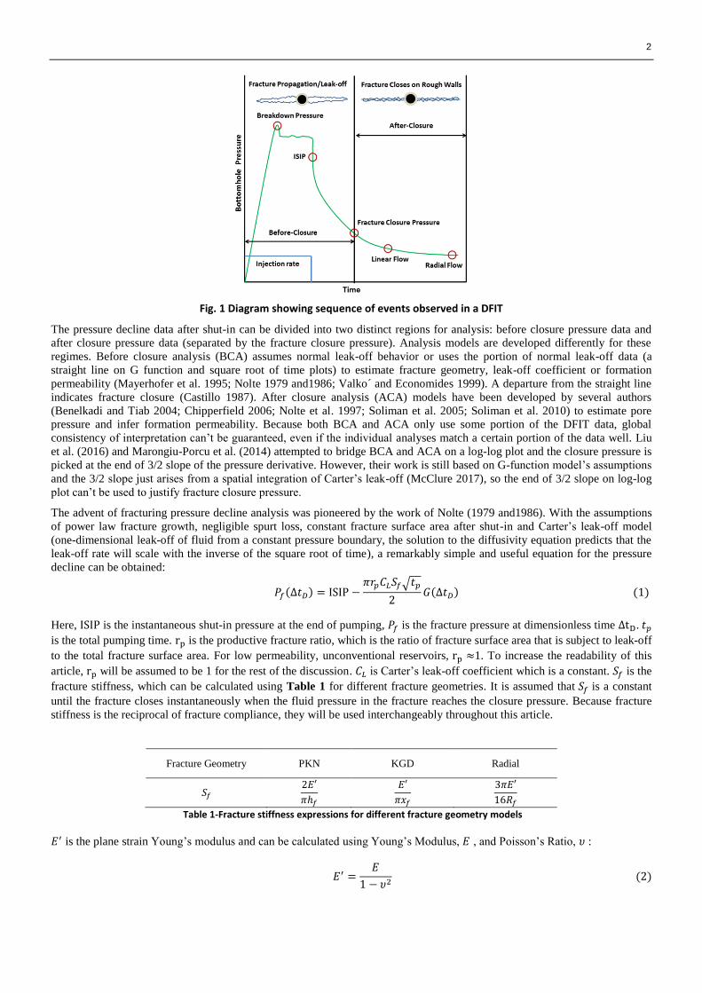
analyzed to obtain in-situ stresses and reservoir properties. A typical pressure trend is qualitatively shown in Fig.1.

Conventionally, DFIT analysis has focused on acquiring fracturing treatment design parameters, such as fluid efficiencies,

leak-off coefficient and fracture closure pressure (which is normally interpreted as minimum in-situ stress). However, in recent

years, DFIT analysis has been extended to obtain reservoir properties such as reservoir pore pressure, and permeability in

unconventional reservoirs, where traditional pressure transient tests are impractical. The reservoir properties determined by

DFIT are representative, because the created fracture can pass through near-wellbore damage zone and provide a large volume

of investigation for true formation properties. In addition, the net pressure trends in a DFIT can be also used to infer the

induced fracture complexity in different geological settings (Potocki 2012). Thoese valuable information obtained from DFITs

provides key input parameters for modeling hydraulic fracture propagation (Wang 2015; Wang 2016; Wang et al. 2016),

stimulation design (Ramurthy et al. 2011), development of reservoir models (Mirani et al. 2016; Loughry et al. 2015; Wang

2017) and post-fracture analysis (Fu et al. 2017). Without a realistic estimation of the fracturing parameters and reservoir

properties, it would not be possible to optimize hydraulic fracture design and evaluate the economic viability of producing

hydrocarbons from unconventional reservoirs.

2

Fig. 1 Diagram showing sequence of events observed in a DFIT

The pressure decline data after shut-in can be divided into two distinct regions for analysis: before closure pressure data and

after closure pressure data (separated by the fracture closure pressure). Analysis models are developed differently for these

regimes. Before closure analysis (BCA) assumes normal leak-off behavior or uses the portion of normal leak-off data (a

straight line on G function and square root of time plots) to estimate fracture geometry, leak-off coefficient or formation

permeability (Mayerhofer et al. 1995; Nolte 1979 and1986; Valko ́and Economides 1999). A departure from the straight line

indicates fracture closure (Castillo 1987). After closure analysis (ACA) models have been developed by several authors

(Benelkadi and Tiab 2004; Chipperfield 2006; Nolte et al. 1997; Soliman et al. 2005; Soliman et al. 2010) to estimate pore

pressure and infer formation permeability. Because both BCA and ACA only use some portion of the DFIT data, global

consistency of interpretation can’t be guaranteed, even if the individual analyses match a certain portion of the data well. Liu

et al. (2016) and Marongiu-Porcu et al. (2014) attempted to bridge BCA and ACA on a log-log plot and the closure pressure is

picked at the end of 3/2 slope of the pressure derivative. However, their work is still based on G-function model’s assumptions

and the 3/2 slope just arises from a spatial integration of Carter’s leak-off (McClure 2017), so the end of 3/2 slope on log-log

plot can’t be used to justify fracture closure pressure.

The advent of fracturing pressure decline analysis was pioneered by the work of Nolte (1979 and1986). With the assumptions

of power law fracture growth, negligible spurt loss, constant fracture surface area after shut-in and Carter’s leak-off model

(one-dimensional leak-off of fluid from a constant pressure boundary, the solution to the diffusivity equation predicts that the

leak-off rate will scale with the inverse of the square root of time), a remarkably simple and useful equation for the pressure

decline can be obtained:

𝑃𝑓(∆𝑡𝐷) = ISIP −𝜋𝑟𝑝𝐶𝐿𝑆𝑓√𝑡𝑝

2𝐺(∆𝑡𝐷) (1)

Here, ISIP is the instantaneous shut-in pressure at the end of pumping, 𝑃𝑓 is the fracture pressure at dimensionless time ∆tD. 𝑡𝑝

is the total pumping time. rp is the productive fracture ratio, which is the ratio of fracture surface area that is subject to leak-off

to the total fracture surface area. For low permeability, unconventional reservoirs, rp ≈1. To increase the readability of this

article, rp will be assumed to be 1 for the rest of the discussion. 𝐶𝐿 is Carter’s leak-off coefficient which is a constant. 𝑆𝑓 is the

fracture stiffness, which can be calculated using Table 1 for different fracture geometries. It is assumed that 𝑆𝑓 is a constant

until the fracture closes instantaneously when the fluid pressure in the fracture reaches the closure pressure. Because fracture

stiffness is the reciprocal of fracture compliance, they will be used interchangeably throughout this article.

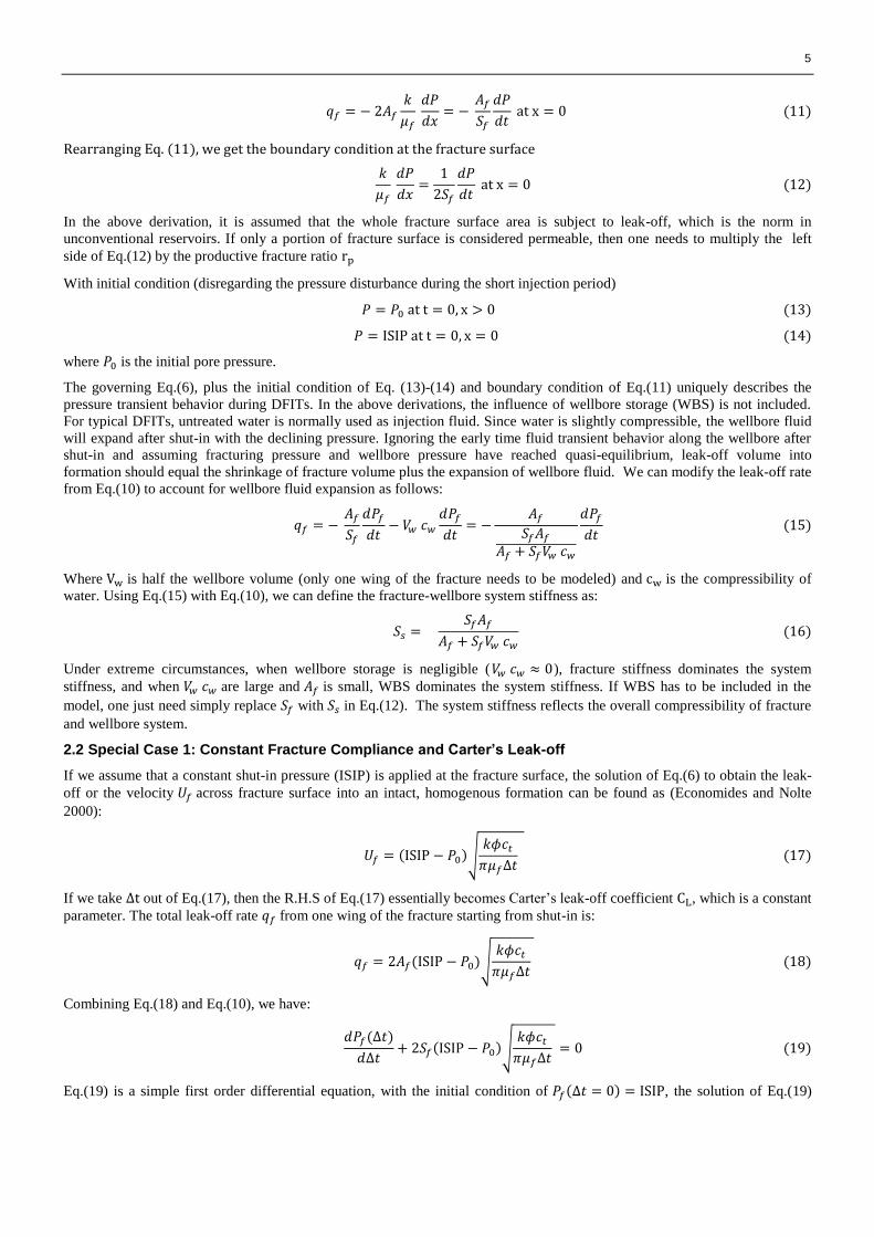
Fracture Geometry PKN KGD Radial

𝑆𝑓 2𝐸′

𝜋ℎ𝑓

𝐸′

𝜋𝑥𝑓

3𝜋𝐸′

16𝑅𝑓

Table 1-Fracture stiffness expressions for different fracture geometry models

𝐸′ is the plane strain Young’s modulus and can be calculated using Young’s Modulus, 𝐸 , and Poisson’s Ratio, 𝜐 :

𝐸′ =𝐸

1 − 𝜐2 (2)

3

The dimensionless time ΔtD is defined by:

𝛥𝑡𝐷 =𝛥𝑡

𝑡𝑒

=𝑡 − 𝑡𝑒

𝑡𝑒

(3)

Where t is the generic time and te is the time at the end of pumping. G-function is defined as

G(ΔtD) =4

π[g(ΔtD) − g(0)] (4)

Where the g-function of time is approximated by,

g(ΔtD) = {(1 + ΔtD)sin−1(1 + ΔtD)−1/2 + ΔtD

1/2 for low fluid efficiency4

3[(1 + ΔtD)1.5 − ΔtD

1.5] for high fluid efficiency (5)

From Eq.(1), we can infer that for normal leak-off behavior (constant Carter’s leak-off coefficient, constant leak-off area and

constant fracture stiffness during fracture closure), the pressure declines linearly with G(∆tD). Castillo (1987) used Nolte's G-

function for modeling the pressure decline behavior and developed the straight-line plot of the G-function vs. pressure. The

slope of this curve is used for the computation of the leak-off coefficient that is independent of pressure. Any departure from

this straight-line is interpreted as closure of the fracture.

Unfortunately, plots of pressure versus G-function often yield curves with multiple points of inflection that have been

attributed to abnormal leak-off behavior (such as pressure dependent leak-off, fracture height recession, closing of secondary

transverse fractures, and fracture tip extension), which makes it difficult to interpret the changes in slope and identify fracture

closure. So identification of fracture closure pressure and non-ideal behavior is usually done using plots of pressure and

GdP/dG versus G-function (Barree and Mukherjee, 1996; Barree, 1998, Barree et al., 2014), where the closure is picked at the

tangential point between a straight line that passes the origin and the GdP/dG curve. This prevailing method of determining

minimum in-situ stress (although has been widely accepted, but has never been theoretically proved) will be classified and

discussed as “tangent line method” in the following text. The fracturing pressure decline model that underlying G-function plot

suffers from two distinct and important issues: (1) leak-off is not pressure-dependent, i.e. a constant pressure boundary is

assumed (2) fracture compliance/stiffness is assumed to be constant during fracture closure. This is why G-function based

models are only used for before closure analysis and are not capable of analyzing DFIT data from the end of pumping to days

or even weeks after shut-in, which requires bridging both before and after closure data seamlessly.

McClure et al. (2016) modeled fracture closure behavior using a fully coupled numerical simulator and found that the “tangent

line method” can severely underestimate closure pressure, and based on the simulation results, they proposed a “compliance

method” for picking closure pressure on the G-function plot, where closure pressure is picked at the point where the fracture

stiffness starts to increase. Zanganeh et al (2017) presented a cohesive zone fracture model to investigate fracture closure

behavior, and their results also show that using the “tangent line method” or using the end of 3/2 slope on a log-log plot can

underestimate closure pressure, and that the “compliance method” is a more reliable approach. However, fracture stiffness (or

compliance) can change continuously during the fracture closure process, because the fracture does not close all at once, but

rather closes on asperities progressively from its edges to the center (Wang and Sharma 2017; Wang et al 2017). So the

mechanical closure pressure identified by “compliance method” can be larger than the minimum principal stress.

To better understanding how fracture stiffness, in-situ stress and pressure dependent leak-off impact the pressure decline

signature, a global DFIT model that is able to simulate pressure decline under a single, coherent mathematic framework, and

correctly capture the variable fracture compliance during closure is needed, and currently, no such model is available. In this

study, we present a generalization of the pressure transient model that couples the fluid pressure in the fracture with a pressure

dependent leak-off rate and variable fracture compliance. Past models will be shown to be special cases for this general

approach under certain simplifying assumptions..

2. Mathematical Formulation

2.1 The General Equations for a Global DFIT Model

The transient pressure response during fracture closure is derived using the following assumptions:

1. Reservoir is isotropic and homogeneous and contains a singlef slightly compressible fluid.

2. Reservoir permeability is low so that poroelastic effects caused by fluid leak-off are negligible

4

3. Fracture surface area subject to leak-off remains constant during and after closure. There are two stages of fracture

closure: mechanical closure, where the fracture surfaces come into contact at asperities, and the other is hydraulic

closure, where fracture pressure in the closed section is disconnected from the open section or wellbore pressure. In the

following derivations, we assume that the mechanically closed fracture still retains hydraulic conductivity because of

its residual fracture width that supported by asperities that caused by erosion or distortion of fracture walls.

4. Fracture has infinite conductivity after closure and pressure is uniformly distributed inside the fracture. This is the

typical case in unconventional reservoirs. And in such case, the pressure distribution inside fracture can be considered

as uniform during closure, as discussed by Koning et al. (1985)

5. The pressure disturbance caused by fracture propagation is negligible. This means that fluid leak-off during pumping is

very small and the duration of injection is very short (typically 3-5 minutes) while the total shut-in time can be hours,

days or even weeks.

In order to correctly capture fracturing pressure response during a DFIT, the pressure dependent leak-off at the fracture surface

and the dynamic changes of fracture compliance during closure have to be accounted for. Fig.2 illustrates one-dimensional

leak-off into a semi-infinite formation.

Fig. 2 Illustration of one-dimensional leak-off

Assuming linear Darcy flow and a slightly compressible, single phase fluid in the reservoir, the differential form of the mass

balance can be written as:

𝜇𝑓𝜙𝑐𝑡

k

∂P

∂t=

∂2P

∂x2 (6)

where 𝑃 is the pressure, k is formation permeability, 𝜇𝑓 is fluid viscosity, 𝜙 is formation porosity and 𝑐𝑡 is total formation

compressibility. Inside the fracture, the average fracture width �̅�𝑓 and fracturing net pressure 𝑃𝑛𝑒𝑡 is related by the fracture

stiffness:

𝑃𝑛𝑒𝑡 = 𝑆𝑓�̅�𝑓 (7)

From a material balance perspective (fluid compressibility is negligible compared to that of the fracture), the rate of fluid leak-

off into the formation, 𝑞𝑓 (one wing of the fracture), after shut-in equals the rate of shrinkage of fracture volume, 𝑉𝑓(one wing

of the fracture), as pressure declines:

𝑞𝑓 = − 𝑑𝑉𝑓

𝑑𝑡 (8)

And

𝑑𝑉𝑓

𝑑𝑡=

𝑑𝐴𝑓�̅�𝑓

𝑑𝑡=

𝐴𝑓

𝑆𝑓

𝑑𝑃𝑛𝑒𝑡

𝑑𝑡=

𝐴𝑓

𝑆𝑓

𝑑𝑃𝑓

𝑑𝑡 (9)

where 𝐴𝑓 is the fracture surface area of one face of one wing of the fracture. So Eq.(8) can be re-written as

𝑞𝑓 = − 𝐴𝑓

𝑆𝑓

𝑑𝑃𝑓

𝑑𝑡 (10)

From the definition, we can conclude that the fracture stiffness (or compliance) is a representation of fracture compressibility

per surface area. Higher stiffness (or lower compliance) implies that the fracture is less compressible. At the boundary of the

fracture surface, both Darcy’s flow and material balance have to be honored

5

𝑞𝑓 = − 2𝐴𝑓

𝑘

𝜇𝑓

𝑑𝑃

𝑑𝑥= −

𝐴𝑓

𝑆𝑓

𝑑𝑃

𝑑𝑡 at x = 0 (11)

Rearranging Eq. (11), we get the boundary condition at the fracture surface

𝑘

𝜇𝑓

𝑑𝑃

𝑑𝑥=

1

2𝑆𝑓

𝑑𝑃

𝑑𝑡 at x = 0 (12)

In the above derivation, it is assumed that the whole fracture surface area is subject to leak-off, which is the norm in

unconventional reservoirs. If only a portion of fracture surface is considered permeable, then one needs to multiply the left

side of Eq.(12) by the productive fracture ratio rp

With initial condition (disregarding the pressure disturbance during the short injection period)

𝑃 = 𝑃0 at t = 0, x > 0 (13)

𝑃 = ISIP at t = 0, x = 0 (14)

where 𝑃0 is the initial pore pressure.

The governing Eq.(6), plus the initial condition of Eq. (13)-(14) and boundary condition of Eq.(11) uniquely describes the

pressure transient behavior during DFITs. In the above derivations, the influence of wellbore storage (WBS) is not included.

For typical DFITs, untreated water is normally used as injection fluid. Since water is slightly compressible, the wellbore fluid

will expand after shut-in with the declining pressure. Ignoring the early time fluid transient behavior along the wellbore after

shut-in and assuming fracturing pressure and wellbore pressure have reached quasi-equilibrium, leak-off volume into

formation should equal the shrinkage of fracture volume plus the expansion of wellbore fluid. We can modify the leak-off rate

from Eq.(10) to account for wellbore fluid expansion as follows:

𝑞𝑓 = − 𝐴𝑓

𝑆𝑓

𝑑𝑃𝑓

𝑑𝑡− 𝑉𝑤 𝑐𝑤

𝑑𝑃𝑓

𝑑𝑡= −

𝐴𝑓

𝑆𝑓𝐴𝑓

𝐴𝑓 + 𝑆𝑓𝑉𝑤 𝑐𝑤

𝑑𝑃𝑓

𝑑𝑡 (15)

Where Vw is half the wellbore volume (only one wing of the fracture needs to be modeled) and cw is the compressibility of

water. Using Eq.(15) with Eq.(10), we can define the fracture-wellbore system stiffness as:

𝑆𝑠 = 𝑆𝑓𝐴𝑓

𝐴𝑓 + 𝑆𝑓𝑉𝑤 𝑐𝑤

(16)

Under extreme circumstances, when wellbore storage is negligible (𝑉𝑤 𝑐𝑤 ≈ 0), fracture stiffness dominates the system

stiffness, and when 𝑉𝑤 𝑐𝑤 are large and 𝐴𝑓 is small, WBS dominates the system stiffness. If WBS has to be included in the

model, one just need simply replace 𝑆𝑓 with 𝑆𝑠 in Eq.(12). The system stiffness reflects the overall compressibility of fracture

and wellbore system.

2.2 Special Case 1: Constant Fracture Compliance and Carter’s Leak-off

If we assume that a constant shut-in pressure (ISIP) is applied at the fracture surface, the solution of Eq.(6) to obtain the leak-

off or the velocity 𝑈𝑓 across fracture surface into an intact, homogenous formation can be found as (Economides and Nolte

2000):

𝑈𝑓 = (ISIP − 𝑃0)√𝑘𝜙𝑐𝑡

𝜋𝜇𝑓∆𝑡 (17)

If we take ∆t out of Eq.(17), then the R.H.S of Eq.(17) essentially becomes Carter’s leak-off coefficient CL, which is a constant

parameter. The total leak-off rate 𝑞𝑓 from one wing of the fracture starting from shut-in is:

𝑞𝑓 = 2𝐴𝑓(ISIP − 𝑃0)√𝑘𝜙𝑐𝑡

𝜋𝜇𝑓∆𝑡 (18)

Combining Eq.(18) and Eq.(10), we have:

𝑑𝑃𝑓(∆𝑡)

𝑑∆𝑡+ 2𝑆𝑓(ISIP − 𝑃0)√

𝑘𝜙𝑐𝑡

𝜋𝜇𝑓∆𝑡 = 0 (19)

Eq.(19) is a simple first order differential equation, with the initial condition of 𝑃𝑓(∆𝑡 = 0) = ISIP, the solution of Eq.(19)

6

leads to the pressure declining proportionally to the square root of time:

𝑃𝑓(∆𝑡) = ISIP − 4𝑆𝑓(ISIP − 𝑃0)√𝑘𝜙𝑐𝑡∆𝑡

𝜋𝜇𝑓

(20)

Eq.(20) is the fundamental basis for the square root of time plot, which is equivalent to Notle’s G-function model. From Eq.(1)

and (20), we can infer that for normal-leak-off behavior with constant fracture stiffness and assuming Carter’s leak-off, the

pressure and its derivative will be straight lines on both G-function and the square root of time plots. However, a closer

observation at Eq.(1) and Eq.(20), we can infer that the fracture pressure continues declining even when it reaches the initial

reservoir pore pressure. This non-physical prediction indicates that the assumption of Carter’s leak-off and constant stiffness

made in the derivation prevent Notle’s G-function model and the square root of time model from capturing the actual pressure

response during fracture closure and late time pressure transient behavior.

2.3: Constant Fracture Compliance and Fracture Pressure Dependent Leak-off

When the leak-off rate is fracture pressure dependent, a closed analytic form of pressure decline is not available, but the

solution can be obtained using a superposition time. A detailed derivation of the pressure decline solution is presented in

Appendix . The fracture pressure at the nth

time interval, 𝑃𝑓,𝑛, can be calculated explicitly:

𝑃𝑓,𝑛 = ISIP − 4𝑆𝑓√𝑘𝜙𝑐𝑡

𝜋𝜇𝑓

∑ ∑(𝑃𝑓,𝑗 − 𝑃𝑓,𝑗−1)(√∆𝑡𝑛 − ∆𝑡𝑗−1

𝑛−1

𝑗=1

𝑛−1

𝑛=1

− √∆𝑡𝑛−1 − ∆𝑡𝑗−1 ) (21)

where 𝑃𝑓,0 = 𝑃0, 𝑃𝑓,1 = 𝐼𝑆𝐼𝑃 , ∆𝑡1 = 0. It is important to note that in this article, the term “fracture pressure dependent leak-

off” (FPDL) specifically refers to a leak-off rate that depends on the declining fluid pressure inside the fracture, not to how the

leak-off rate changes with net stress in the rock surrounding the fracture, which is often denoted as pressure dependent leak-off

or PDL (Barree et al. 2009). In some cases, excessive pressure drop can be observed during early-time of shut-in in low

permeability reservoirs, but it is the result of high apparent ISIP, wellbore storage and additional friction away from the

wellbore, and not caused by PDL, which is unlikely to happen in unconventional reservoirs.

2.4 Variable Fracture Compliance

2.4.1 The Cause of Variable Fracture Compliance

There are basically two main causes that lead the continuously changing of fracture compliance during closure. The first is

stress contrast across different layers that the fracture has penetrated into. In this case, fracture will close first in the zones

where the minimum in-situ stress is highest, which alters the overall fracture stiffness during the closure process. The second

cause of variable fracture compliance is fracture surface asperities and roughness, where the fracture closes on asperities

progressively from its edges to the center, and the overall fracture stiffness is determined by both the closed portion and open

portion of fracture during closure.

As pressure declines inside the fracture after shut-in, the fracture will gradually close and the fracture aperture will approach

the scale of the surface roughness. If the fracture faces are perfectly parallel and smooth, they will come into contact all at

once when the fluid pressure inside the fracture declines to the far field stress, and the fracture is then mechanically and

hydraulically closed. However, there is abundant evidence to suggest that fractures retain their conductivity after the walls

have come into contact (mechanical closure). Fractures retain a finite aperture after mechanical closure due to a mismatch of

asperities on the fracture walls. van Dam et al. (2000) presented scaled laboratory experiments on hydraulic fracture closure

behavior. They observed up to a 15% residual aperture (compared to the maximum aperture during fracture propagation) long

after shut-in. Fredd et al. (2000) demonstrated fracture surface asperities can provide residual fracture width and sufficient

conductivity in the absence of proppants. Using sandstone cores from the East Texas Cotton Valley formation, sheared fracture

surface asperities that had an average height of about 2.286 mm were observed. Warpinski et al. (1993) reported hydraulic

fracture surface asperities of about 1.016 mm and 4.064 mm for nearly homogeneous sandstones and sandstones with coal and

clay-rich bedding planes, respectively. Sakaguchi et al. (2008) created tensile fractures in large rock blocks and measured the

asperity height and distribution. Their work shows that the fracture surfaces can be assumed to be a fractal object and most of

the asperities fall within 1 to 2 mm in height. Wells and Davatzes (2015) conducted topographic measurement on dilated

fractures from core samples and found the asperity height ranges from hundreds to thousands of micrometers. Bhide et al.

(2014) created X-ray microtomographic images from shear induced fractures and the roughness values obtained varied from

1.8 to 1.95 mm along the length of the rock samples. Zou et al. (2015) conducted experiments on 20 fractured shale samples

and found the average asperity height to be 1.88 mm. An experimental study (Zhang et al. 2014) on Barnett Shale samples

reveals that the surface topography of the displaced fracture can be altered because of rock failure, and the fracture surface

exhibited parallel strips of crushed asperities. Field measurements (Warpinski et al. 2002) using a down-hole tiltmeter array

7

indicated that the fracture closure process is a smooth, continuous one which often leaves 20%-30% residual fracture width,

regardless of whether the injection fluid is water, linear-gel or cross-linked-gel.

The microscopic measurement and modeling of surface roughness and mechanical properties of asperities can often be up-

scaled to macroscopic contact laws that relate fracture width and the associated contact stress. Willis-Richards et al. (1996)

proposed contact law to relate fracture width and the net closure stress for fractured rocks, based on the work of Barton et al.

(1985):

𝜎𝑐 =𝜎𝑟𝑒𝑓

9(

𝑤0

𝑤𝑓− 1) for 𝑤𝑓 ≤ 𝑤0 (22)

where 𝑤𝑓 is the fracture aperture and, 𝑤0 is the contact width, which represents the fracture aperture when the contact normal

stress is equal to zero, 𝜎𝑐 is the contact normal stress on the fracture, and 𝜎𝑟𝑒𝑓 is a contact reference stress, which denotes the

effective normal stress at which the aperture is reduced by 90%. it should be emphasized that the contact width 𝑤0 is

determined by the tallest asperities, and the strength, spatial and height distribution of asperities are reflected by the contact

reference stress 𝜎𝑟𝑒𝑓 (e.g., if the tallest asperities on two fracture samples are the same, then they should have the same 𝑤0, but

the one with a higher median asperity height or Young’s modulus will have higher value of 𝜎𝑟𝑒𝑓 , provided other properties are

the same).

2.4.2 Determine Pressure Dependent Fracture Compliance

With known fracture geometry, rock properties and surface roughness (represented by contact parameters w0 and σref), the

question now is how to estimate fracture stiffness (or compliance) as a function of pressure, if it continuously changes during

fracture closure. Once the pressure dependent fracture stiffness is obtained, it can be substituted into Eq.(12) and the whole

system of equations can be solved readily. Wang and Sharma (2017) presented an integral transform method and general

algorithms to model the dynamic behavior of hydraulic fracture closure on rough fracture surfaces and asperities, using linear

elastic solutions that coupled with contact law for three different fracture models (PKN, KGD and radial fracture geometry).

Given the fracture geometry, rock properties, contact parameters and minimum principal stress, their approach can predict the

evolution of fracture aperture profile, total fracture volume and fracture stiffness as fracturing pressure declines. Wang et al.

(2017) presented an improved model for fracture closure based on superposition principles. Their model can simulate large

scale fracture closure behavior with layer stress contrast in an efficient manner.

Detailed modeling of non-local fracture closure on asperities and rough surfaces has already been discussed extensively (Wang

and Sharma 2017; Wang et al. 2017), hence will not be discuss further. Here, we’ll examine an example of a fracture that

closes on asperities and how the fracture stiffness evolves during closure. Assuming a Young's modulus of 20 GPa, Poisson's

ratio of 0.25, 𝑤0 of 2 mm, 𝜎𝑟𝑒𝑓 of 5 MPa for a PKN fracture geometry with 10 m fracture height, 35 MPa minimum in-situ

stress, the evolution of the fracture width profile and contact stress distribution can be determined, as the fluid pressure inside

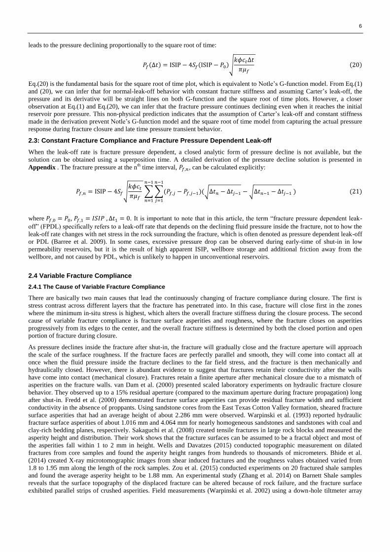
the fracture gradually declines. The results are shown in Fig.3 and Fig.4. To demonstrate the impact of fracture roughness and

surface asperities on fracture closure behavior, the case without surface asperities (fracture surface is completely planar and

smooth) is also included. The result shows that at relative high fracturing fluid pressure, the fracture asperities have negligible

impact on fracture width distribution, and the contact stress is always concentrated at the tip of the fracture, where the contact

stress is much higher than in the middle of the fracture. We can also see that the fracture surfaces do not contact each other like

parallel plates. In fact, the fracture closes on rough surfaces starting from the tip, and closes progressively all the way from the

edges to the center of fracture. As fluid pressure continues to decline, more and more of the fracture surfaces come into contact

and these changes the subsequent fracture closure behavior. At lower fluid pressures, contact stresses start to counter-balance

the in-situ stress and the fracture becomes stiffer and less compliant. If the fracture faces were perfectly parallel and smooth,

the fracture width would have collapsed to zero when the fluid pressure dropped to 35 MPa. The moment when all fracture

surfaces come into contact on asperities and the contact stress becomes non-zero on the entire fracture surface, the fracture is

mechanically closed and this mechanical closure stress is higher than the minimum in-situ stress.

8

Fig.3 Fracture width evolution with and without asperities at different fluid pressure for a PKN geometry

Fig.4 Fracture width and the corresponding contact stress distribution at different fluid pressure for a PKN geometry

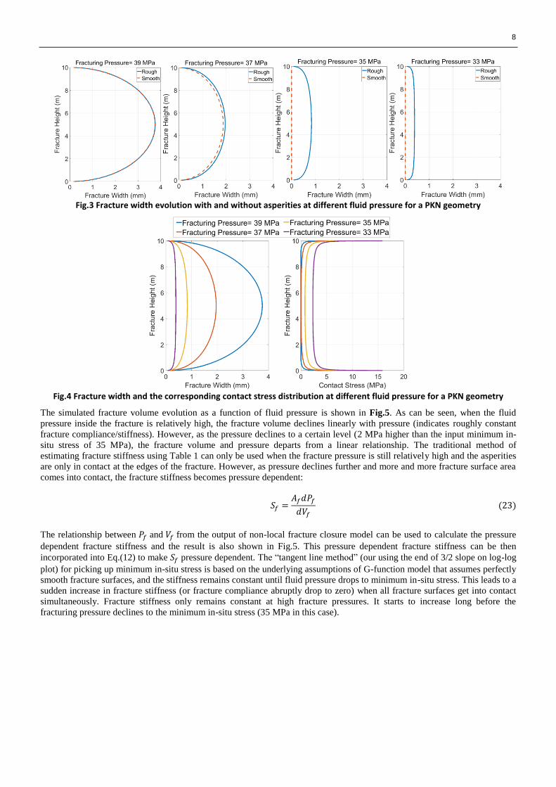
The simulated fracture volume evolution as a function of fluid pressure is shown in Fig.5. As can be seen, when the fluid

pressure inside the fracture is relatively high, the fracture volume declines linearly with pressure (indicates roughly constant

fracture compliance/stiffness). However, as the pressure declines to a certain level (2 MPa higher than the input minimum in-

situ stress of 35 MPa), the fracture volume and pressure departs from a linear relationship. The traditional method of

estimating fracture stiffness using Table 1 can only be used when the fracture pressure is still relatively high and the asperities

are only in contact at the edges of the fracture. However, as pressure declines further and more and more fracture surface area

comes into contact, the fracture stiffness becomes pressure dependent:

𝑆𝑓 =𝐴𝑓𝑑𝑃𝑓

𝑑𝑉𝑓

(23)

The relationship between 𝑃𝑓 and 𝑉𝑓 from the output of non-local fracture closure model can be used to calculate the pressure

dependent fracture stiffness and the result is also shown in Fig.5. This pressure dependent fracture stiffness can be then

incorporated into Eq.(12) to make 𝑆𝑓 pressure dependent. The “tangent line method” (our using the end of 3/2 slope on log-log

plot) for picking up minimum in-situ stress is based on the underlying assumptions of G-function model that assumes perfectly

smooth fracture surfaces, and the stiffness remains constant until fluid pressure drops to minimum in-situ stress. This leads to a

sudden increase in fracture stiffness (or fracture compliance abruptly drop to zero) when all fracture surfaces get into contact

simultaneously. Fracture stiffness only remains constant at high fracture pressures. It starts to increase long before the

fracturing pressure declines to the minimum in-situ stress (35 MPa in this case).

9

Fig.5 Fracture volume and fracture stiffness evolution as fluid pressure declines for a PKN geometry

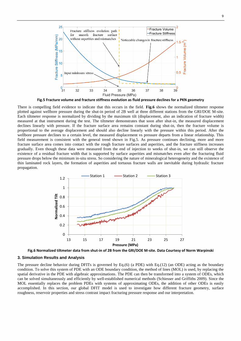
There is compelling field evidence to indicate that this occurs in the field. Fig.6 shows the normalized tiltmeter response

plotted against wellbore pressure during the shut-in period of 2B well at three different stations from the GRI/DOE M-site.

Each tiltmeter response is normalized by dividing by the maximum tilt (displacement, also an indication of fracture width)

measured at that instrument during the test. The tiltmeter demonstrates that soon after shut-in, the measured displacement

declines linearly with pressure. If the fracture surface area remains constant during shut-in, then the fracture volume is

proportional to the average displacement and should also decline linearly with the pressure within this period. After the

wellbore pressure declines to a certain level, the measured displacement vs pressure departs from a linear relationship. This

field measurement is consistent with the general trend shown in Fig.5. As pressure continues declining, more and more

fracture surface area comes into contact with the rough fracture surfaces and asperities, and the fracture stiffness increases

gradually. Even though these data were measured from the end of injection to weeks of shut-in, we can still observe the

existence of a residual fracture width that is supported by surface asperities and mismatches even after the fracturing fluid

pressure drops below the minimum in-situ stress. So considering the nature of mineralogical heterogeneity and the existence of

thin laminated rock layers, the formation of asperities and tortuous fracture walls are inevitable during hydraulic fracture

propagation.

Fig.6 Normalized tiltmeter data from shut-in of 2B from the GRI/DOE M-site. Data Courtesy of Norm Warpinski

3. Simulation Results and Analysis

The pressure decline behavior during DFITs is governed by Eq.(6) (a PDE) with Eq.(12) (an ODE) acting as the boundary

condition. To solve this system of PDE with an ODE boundary condition, the method of lines (MOL) is used, by replacing the

spatial derivative in the PDE with algebraic approximations. The PDE can then be transformed into a system of ODEs, which

can be solved simultaneously and efficiently by well-established numerical methods (Schiesser and Griffiths 2009). Since the

MOL essentially replaces the problem PDEs with systems of approximating ODEs, the addition of other ODEs is easily

accomplished. In this section, our global DFIT model is used to investigate how different fracture geometry, surface

roughness, reservoir properties and stress contrast impact fracturing pressure response and our interpretation.

0

0.2

0.4

0.6

0.8

1

1.2

13 15 17 19 21 23 25 27

No

rmal

ize

d T

ilt

Pressure (MPa)

Station 1 Station 2 Station 3

10

3.1 Normal leak-off behavior

Normal leak-off behavior is a special case of our model that satisfies all the assumptions of Nolte’s G-function model, and it

can be clearly identified with straight lines of pressure and its derivatives on G-function and the square root of time plots. All

previous BCA models assume that these straight lines indicate normal leak-off behavior and hence, leak-off coefficient or

formation permeability can be determined based on this portion of the data. However, two key assumptions in all BCA are

Carter’s leak-off and constant fracture compliance. To examine the impact of incorrectly assuming Carter’s leak-off for the

duration of the DFIT, we extend the concept of “normal leak-off behavior” to account for different fracture boundary

conditions, while other assumptions remain the same (i.e., constant fracture compliance and constant surface area during

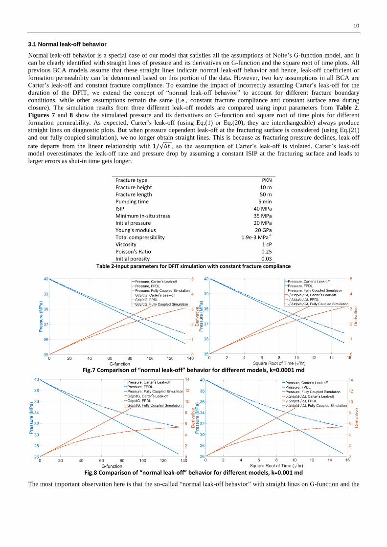
closure). The simulation results from three different leak-off models are compared using input parameters from Table 2.

Figures 7 and 8 show the simulated pressure and its derivatives on G-function and square root of time plots for different

formation permeability. As expected, Carter’s leak-off (using Eq.(1) or Eq.(20), they are interchangeable) always produce

straight lines on diagnostic plots. But when pressure dependent leak-off at the fracturing surface is considered (using Eq.(21)

and our fully coupled simulation), we no longer obtain straight lines. This is because as fracturing pressure declines, leak-off

rate departs from the linear relationship with 1/√∆𝑡 , so the assumption of Carter’s leak-off is violated. Carter’s leak-off

model overestimates the leak-off rate and pressure drop by assuming a constant ISIP at the fracturing surface and leads to

larger errors as shut-in time gets longer.

Fracture type PKN Fracture height 10 m Fracture length 50 m Pumping time 5 min ISIP 40 MPa Minimum in-situ stress 35 MPa Initial pressure 20 MPa Young's modulus 20 GPa Total compressibility 1.9e-3 MPa

-1

Viscosity 1 cP Poisson's Ratio 0.25 Initial porosity 0.03

Table 2-Input parameters for DFIT simulation with constant fracture compliance

Fig.7 Comparison of “normal leak-off” behavior for different models, k=0.0001 md

Fig.8 Comparison of “normal leak-off” behavior for different models, k=0.001 md

The most important observation here is that the so-called “normal leak-off behavior” with straight lines on G-function and the

11

square root of time plots is not “normal” at all. For example, the closure time for typical DFIT in a formation with 0.0001 md

permeability is around 2~4 days. And in the above case shown in Fig.7, the fracturing pressure and its derivative depart from

the straight line after 4 hours of shut-in, even with constant fracture compliance/stiffness, surface area and reservoir properties.

Many field data sets do show “normal leak-off behavior” with straight lines that extend all the way to the point of downward

deflection. This occurs if some mechanisms that accelerate pressure drop (e.g., the gradual increase of fracture stiffness)

happen to offset the effects of declining pressure at the fracture surface, so the pressure data fits the straight lines predicted by

Carter’s leak-off model coincidentally. So any DFIT analysis that is based on the assumption of Carter’s leak-off and straight

lines on G-function and the square root of time plots should be re-examined.

3.2 Variable Fracture Compliance on Pressure Decline and In-Situ Stress Estimation

As discussed earlier, G-function and previous BCA models assume Carter’s leak-off behavior as if the pressure in the fracture

is a constant value (i.e., ISIP). In addition, these models also assume fracture compliance/stiffness is constant and only changes

abruptly at the moment of fracture closure, when fracturing pressure drops to the minimum in-situ stress. The failure to

account for the coupled mechanisms of pressure dependent leak-off at the fracture surface and the gradual increase of fracture

stiffness during closure explains why these models are only useful on a small portion of the before closure data, and are not

able to simulate the fracturing response for the entire duration of the DFIT test. These simplifying assumptions also make their

interpretation of DFIT data and estimation of minimum in-situ stress inaccurate. In this section, our global DFIT model is used

to investigate how each factor impacts the pressure decline trend and our estimation of minimum in-situ stress and fracture

compliance.

3.2.1 PKN Fracture Geometry

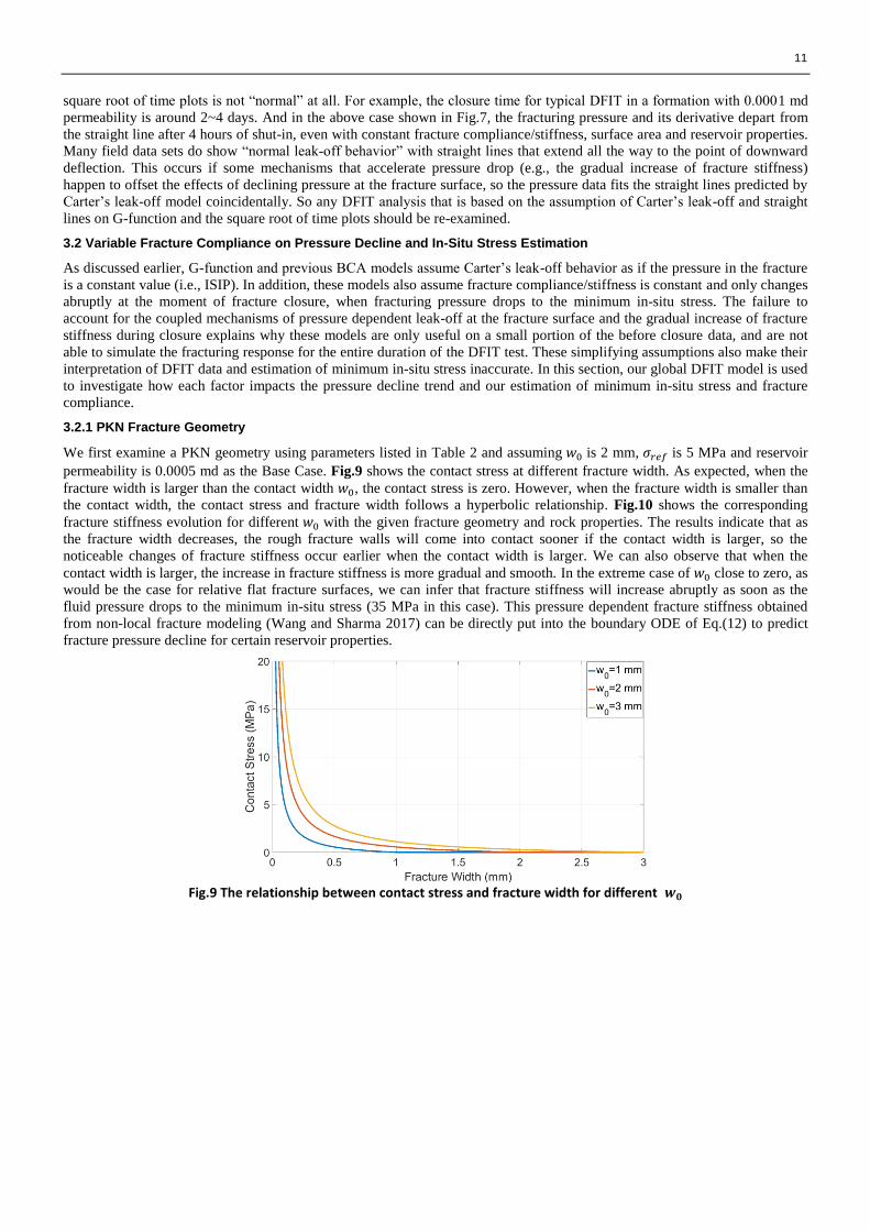
We first examine a PKN geometry using parameters listed in Table 2 and assuming 𝑤0 is 2 mm, 𝜎𝑟𝑒𝑓 is 5 MPa and reservoir

permeability is 0.0005 md as the Base Case. Fig.9 shows the contact stress at different fracture width. As expected, when the

fracture width is larger than the contact width 𝑤0, the contact stress is zero. However, when the fracture width is smaller than

the contact width, the contact stress and fracture width follows a hyperbolic relationship. Fig.10 shows the corresponding

fracture stiffness evolution for different 𝑤0 with the given fracture geometry and rock properties. The results indicate that as

the fracture width decreases, the rough fracture walls will come into contact sooner if the contact width is larger, so the

noticeable changes of fracture stiffness occur earlier when the contact width is larger. We can also observe that when the

contact width is larger, the increase in fracture stiffness is more gradual and smooth. In the extreme case of 𝑤0 close to zero, as

would be the case for relative flat fracture surfaces, we can infer that fracture stiffness will increase abruptly as soon as the

fluid pressure drops to the minimum in-situ stress (35 MPa in this case). This pressure dependent fracture stiffness obtained

from non-local fracture modeling (Wang and Sharma 2017) can be directly put into the boundary ODE of Eq.(12) to predict

fracture pressure decline for certain reservoir properties.

Fig.9 The relationship between contact stress and fracture width for different 𝒘𝟎

12

Fig.10 Fracture stiffness evolution for different 𝒘𝟎 with a PKN geometry

Fig.11 shows the fracturing pressure and its derivatives for different 𝑤0 on G-function and square root of time plots. Relate

with Fig.9 and Fig.10, we can see that the contact width impacts pressure decline response significantly, because it alters the

evolution of fracture stiffness. Large contact width leads to a smooth pressure decline trend while small contact width leads to

steep changes in pressure decline rate and pressure derivatives. We can also infer that if the contact width is close to zero and

all fracture walls come into contact simultaneously, then a sudden change in pressure decline rate and the pressure derivative

spikes on both G-function and square root of time plots are inevitable, which is unrealistic and never observed in field cases.

So the conventional assumption that a fracture closes on flat, smooth fracture surfaces where 𝑤0 = 0 does not reflect reality.

In addition, different contact widths lead to different derivative slopes, so any BCA models that attempt to match this portion

of data and estimate reservoir properties without considering the variable fracture compliance is questionable. Fig.11 also

shows G-function and square root of time plots give the same quantitative information only slightly different in scales. More

importantly, the estimated minimum in-situ stress from pressure derivatives using the “convention method” and “compliance

method” give inconsistent results for different contact widths, with the same input parameters of fracture surface area,

minimum in-situ stress and reservoir properties. A detailed comparison and a new approach to estimate minimum in-situ stress

will be discussed later.

Fig.11 Pressure decline response for different 𝒘𝟎 with a PKN geometry

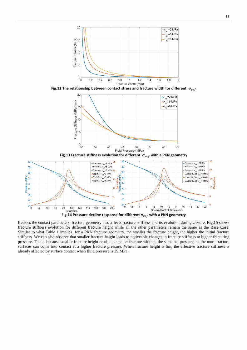
Next, we examine how contact reference stress affects the pressure decline response. Fig.12 and Fig.13 show the relationship

between contact stress and fracture width for different contact reference stress and the corresponding fracture stiffness

evolution at different fracturing pressure. For the same contact width, the higher the contact reference stress, the more rapid

the increase of contact stress as the fracture width shrinks. Physically, the contact reference stress represents how hard and

strong the fracture surface asperities are. The lower the contact reference stress, the more gradual the change in fracture

stiffness as pressure declines. Even though the contact reference stress does not have much impact on the pressure at which the

fracture stiffness starts to changes noticeably, it does impact the fracture stiffness evolution, as shown in Fig.13. Fig.14 shows

the fracturing pressure and its derivatives for different contact reference stress on G-function and the square root of time plots.

It can be observed that the contact reference stress has negligible influence on early time pressure decline when fracturing

pressure is still high. This is because only the fracture edges start to come into contact during this period and the fracture

stiffness remains roughly constant. However, after this period as the fracture pressure declines further, more and more fracture

surfaces come into contact and the contact reference stress begins to affect the pressure decline trend and the peak value of the

pressure derivatives.

13

Fig.12 The relationship between contact stress and fracture width for different 𝝈𝒓𝒆𝒇

Fig.13 Fracture stiffness evolution for different 𝝈𝒓𝒆𝒇 with a PKN geometry

Fig.14 Pressure decline response for different 𝝈𝒓𝒆𝒇 with a PKN geometry

Besides the contact parameters, fracture geometry also affects fracture stiffness and its evolution during closure. Fig.15 shows

fracture stiffness evolution for different fracture height while all the other parameters remain the same as the Base Case.

Similar to what Table 1 implies, for a PKN fracture geometry, the smaller the fracture height, the higher the initial fracture

stiffness. We can also observe that smaller fracture height leads to noticeable changes in fracture stiffness at higher fracturing

pressure. This is because smaller fracture height results in smaller fracture width at the same net pressure, so the more fracture

surfaces can come into contact at a higher fracture pressure. When fracture height is 5m, the effective fracture stiffness is

already affected by surface contact when fluid pressure is 39 MPa.

14

Fig.15 Fracture stiffness evolution for different fracture height with a PKN geometry

Fig.16 shows the fracturing pressure and its derivatives for different fracture height on G-function and the square root of time

plots. The results indicate that fracture height impacts the pressure decline trend significantly. Larger fracture height leads to

later occurrence of the peak of the pressure derivative and this also increases the peak value of the pressure derivatives.

Fig.16 Pressure decline response for different fracture height with a PKN geometry

Fig.17 shows the fracturing pressure and its derivatives for different reservoir permeability on G-function and the square root

of time plots. As expected, the pressure declines more rapidly when the reservoir permeability is large and the decline rate

slows down as the difference between fracturing pressure and initial reservoir pressure becomes smaller and smaller.

Fig.17 Pressure decline response for different reservoir permeability with a PKN geometry

Next, we examine the impact of wellbore storage on the fully coupled pressure decline trend. The water compressibility is

assumed to be 4.35e-4 MPa-1

. Fig.18 shows the fracture-wellbore system stiffness evolution for different wellbore volume. As

can be seen, when fracturing pressure is high, fracture stiffness dominates the system stiffness. However, as fracturing pressure

continues declining, the fracture become less and less compressible and the role of wellbore storage becomes apparent. In

general, the larger the wellbore volume, the more gradual and slower the increase in system stiffness will be.

15

Fig.18 Fracture-wellbore system stiffness evolution for different wellbore volume with a PKN geometry

Fig.19 shows the corresponding fracturing pressure and its derivatives for different wellbore volumes on G-function and

square root of time plots. It can be observed that larger wellbore volume leads to more gradual pressure decline trends. A

larger wellbore volume also delays the occurrence of fracture closure and lowers the peak of the pressure derivative curve. It

can be seen that WBS has a small impact during early time of shut-in when the system stiffness is still dominated by fracture

stiffness, however, as more and more of the fracture surface comes into contact and the fracture becomes stiffer, WBS effects

become apparent, and the after-flow of fluid from wellbore to fracture long after shut-in decelerates the pressure decline rate

and extends the tail of the pressure derivative after its reaches the peak. So the WBS effect on pressure decline response must

be accounted for when interpreting and analyzing DFIT data.

Fig.19 Pressure decline response for different wellbore volume with a PKN geometry

Fig.20 shows the fracturing pressure and its derivatives for different initial reservoir pressure on G-function and square root of

time plots. It can be observed when the initial reservoir pressure is low; the pressure declines more rapidly. This is also

reflected by Eq.(18), a lower reservoir pressure leads to a higher leak-off rate. However, when the reservoir pressure is over

pressurized with high initial pore pressure, the pressure decline trend resembles a “normal-leak-off behavior”. In this case

(𝑃0=28MPa), one can still notice that there exist a subtle “bump” in the pressure derivatives that indicates an increase in

fracture stiffness as reflected in Fig.10. For small values of 𝜎𝑟𝑒𝑓 , this increase can be too gradual to be noticeable on

G-function and square root of time plots. This example demonstrates that long closure time not only can be attributed to low

formation permeability, but also can be the result of a small pressure difference between ISIP and initial pore pressure.

Fig.20 Pressure decline response for different initial reservoir pressure with a PKN geometry

16

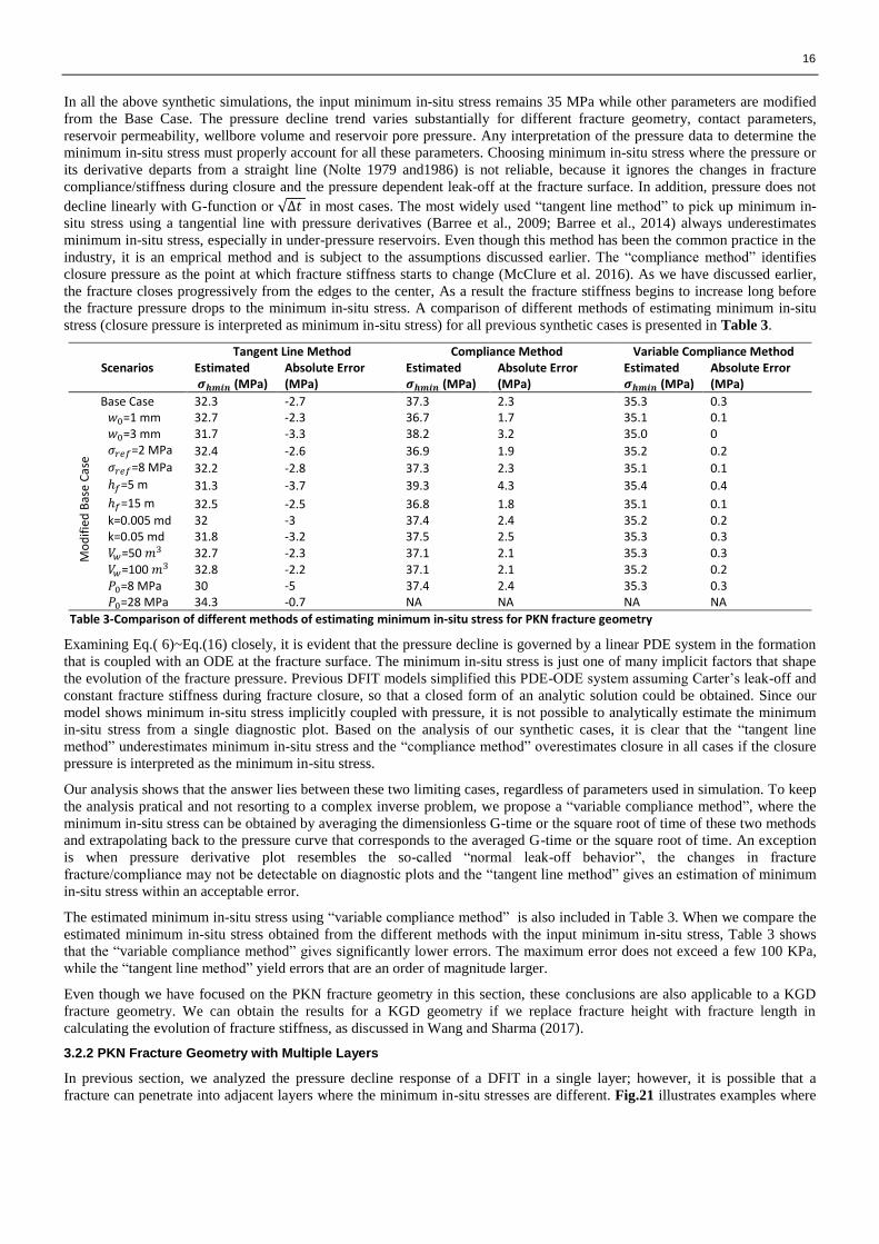
In all the above synthetic simulations, the input minimum in-situ stress remains 35 MPa while other parameters are modified

from the Base Case. The pressure decline trend varies substantially for different fracture geometry, contact parameters,

reservoir permeability, wellbore volume and reservoir pore pressure. Any interpretation of the pressure data to determine the

minimum in-situ stress must properly account for all these parameters. Choosing minimum in-situ stress where the pressure or

its derivative departs from a straight line (Nolte 1979 and1986) is not reliable, because it ignores the changes in fracture

compliance/stiffness during closure and the pressure dependent leak-off at the fracture surface. In addition, pressure does not

decline linearly with G-function or √∆𝑡 in most cases. The most widely used “tangent line method” to pick up minimum in-

situ stress using a tangential line with pressure derivatives (Barree et al., 2009; Barree et al., 2014) always underestimates

minimum in-situ stress, especially in under-pressure reservoirs. Even though this method has been the common practice in the

industry, it is an emprical method and is subject to the assumptions discussed earlier. The “compliance method” identifies

closure pressure as the point at which fracture stiffness starts to change (McClure et al. 2016). As we have discussed earlier,

the fracture closes progressively from the edges to the center, As a result the fracture stiffness begins to increase long before

the fracture pressure drops to the minimum in-situ stress. A comparison of different methods of estimating minimum in-situ

stress (closure pressure is interpreted as minimum in-situ stress) for all previous synthetic cases is presented in Table 3.

Scenarios Tangent Line Method Compliance Method Variable Compliance Method

Estimated 𝝈𝒉𝒎𝒊𝒏 (MPa)

Absolute Error (MPa)

Estimated 𝝈𝒉𝒎𝒊𝒏 (MPa)

Absolute Error (MPa)

Estimated 𝝈𝒉𝒎𝒊𝒏 (MPa)

Absolute Error (MPa)

Base Case 32.3 -2.7 37.3 2.3 35.3 0.3

Mo

dif

ied

Bas

e C

ase

𝑤0=1 mm 32.7 -2.3 36.7 1.7 35.1 0.1 𝑤0=3 mm 31.7 -3.3 38.2 3.2 35.0 0 𝜎𝑟𝑒𝑓=2 MPa 32.4 -2.6 36.9 1.9 35.2 0.2 𝜎𝑟𝑒𝑓=8 MPa 32.2 -2.8 37.3 2.3 35.1 0.1 ℎ𝑓=5 m 31.3 -3.7 39.3 4.3 35.4 0.4

ℎ𝑓=15 m 32.5 -2.5 36.8 1.8 35.1 0.1 k=0.005 md 32 -3 37.4 2.4 35.2 0.2 k=0.05 md 31.8 -3.2 37.5 2.5 35.3 0.3 𝑉𝑤=50 𝑚3 32.7 -2.3 37.1 2.1 35.3 0.3 𝑉𝑤=100 𝑚3 32.8 -2.2 37.1 2.1 35.2 0.2 𝑃0=8 MPa 30 -5 37.4 2.4 35.3 0.3 𝑃0=28 MPa 34.3 -0.7 NA NA NA NA

Table 3-Comparison of different methods of estimating minimum in-situ stress for PKN fracture geometry

Examining Eq.( 6)~Eq.(16) closely, it is evident that the pressure decline is governed by a linear PDE system in the formation

that is coupled with an ODE at the fracture surface. The minimum in-situ stress is just one of many implicit factors that shape

the evolution of the fracture pressure. Previous DFIT models simplified this PDE-ODE system assuming Carter’s leak-off and

constant fracture stiffness during fracture closure, so that a closed form of an analytic solution could be obtained. Since our

model shows minimum in-situ stress implicitly coupled with pressure, it is not possible to analytically estimate the minimum

in-situ stress from a single diagnostic plot. Based on the analysis of our synthetic cases, it is clear that the “tangent line

method” underestimates minimum in-situ stress and the “compliance method” overestimates closure in all cases if the closure

pressure is interpreted as the minimum in-situ stress.

Our analysis shows that the answer lies between these two limiting cases, regardless of parameters used in simulation. To keep

the analysis pratical and not resorting to a complex inverse problem, we propose a “variable compliance method”, where the

minimum in-situ stress can be obtained by averaging the dimensionless G-time or the square root of time of these two methods

and extrapolating back to the pressure curve that corresponds to the averaged G-time or the square root of time. An exception

is when pressure derivative plot resembles the so-called “normal leak-off behavior”, the changes in fracture

fracture/compliance may not be detectable on diagnostic plots and the “tangent line method” gives an estimation of minimum

in-situ stress within an acceptable error.

The estimated minimum in-situ stress using “variable compliance method” is also included in Table 3. When we compare the

estimated minimum in-situ stress obtained from the different methods with the input minimum in-situ stress, Table 3 shows

that the “variable compliance method” gives significantly lower errors. The maximum error does not exceed a few 100 KPa,

while the “tangent line method” yield errors that are an order of magnitude larger.

Even though we have focused on the PKN fracture geometry in this section, these conclusions are also applicable to a KGD

fracture geometry. We can obtain the results for a KGD geometry if we replace fracture height with fracture length in

calculating the evolution of fracture stiffness, as discussed in Wang and Sharma (2017).

3.2.2 PKN Fracture Geometry with Multiple Layers

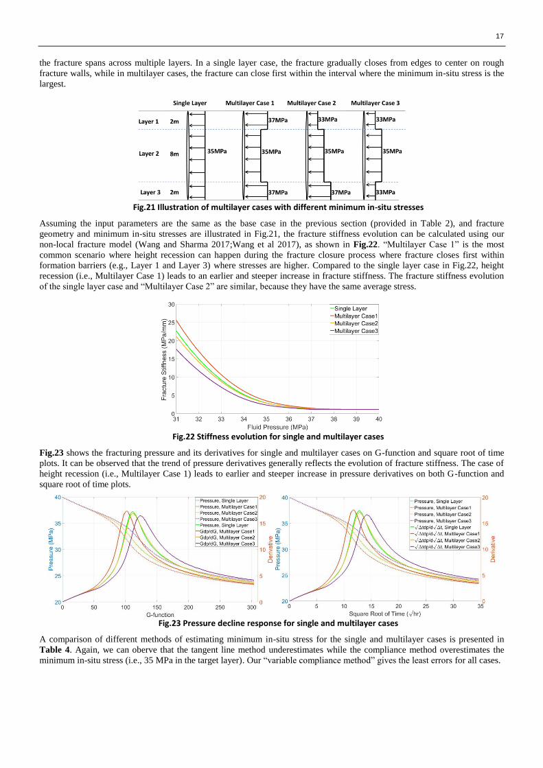
In previous section, we analyzed the pressure decline response of a DFIT in a single layer; however, it is possible that a

fracture can penetrate into adjacent layers where the minimum in-situ stresses are different. Fig.21 illustrates examples where

17

the fracture spans across multiple layers. In a single layer case, the fracture gradually closes from edges to center on rough

fracture walls, while in multilayer cases, the fracture can close first within the interval where the minimum in-situ stress is the

largest.

Fig.21 Illustration of multilayer cases with different minimum in-situ stresses

Assuming the input parameters are the same as the base case in the previous section (provided in Table 2), and fracture

geometry and minimum in-situ stresses are illustrated in Fig.21, the fracture stiffness evolution can be calculated using our

non-local fracture model (Wang and Sharma 2017;Wang et al 2017), as shown in Fig.22. “Multilayer Case 1” is the most

common scenario where height recession can happen during the fracture closure process where fracture closes first within

formation barriers (e.g., Layer 1 and Layer 3) where stresses are higher. Compared to the single layer case in Fig.22, height

recession (i.e., Multilayer Case 1) leads to an earlier and steeper increase in fracture stiffness. The fracture stiffness evolution

of the single layer case and “Multilayer Case 2” are similar, because they have the same average stress.

Fig.22 Stiffness evolution for single and multilayer cases

Fig.23 shows the fracturing pressure and its derivatives for single and multilayer cases on G-function and square root of time

plots. It can be observed that the trend of pressure derivatives generally reflects the evolution of fracture stiffness. The case of

height recession (i.e., Multilayer Case 1) leads to earlier and steeper increase in pressure derivatives on both G-function and

square root of time plots.

Fig.23 Pressure decline response for single and multilayer cases

A comparison of different methods of estimating minimum in-situ stress for the single and multilayer cases is presented in

Table 4. Again, we can oberve that the tangent line method underestimates while the compliance method overestimates the

minimum in-situ stress (i.e., 35 MPa in the target layer). Our “variable compliance method” gives the least errors for all cases.

18

Scenarios

Tangent Line Method Compliance Method Variable Compliance Method

Estimated 𝝈𝒉𝒎𝒊𝒏 (MPa)

Absolute Error (MPa)

Estimated 𝝈𝒉𝒎𝒊𝒏 (MPa)

Absolute Error (MPa)

Estimated 𝝈𝒉𝒎𝒊𝒏 (MPa)

Absolute Error (MPa)

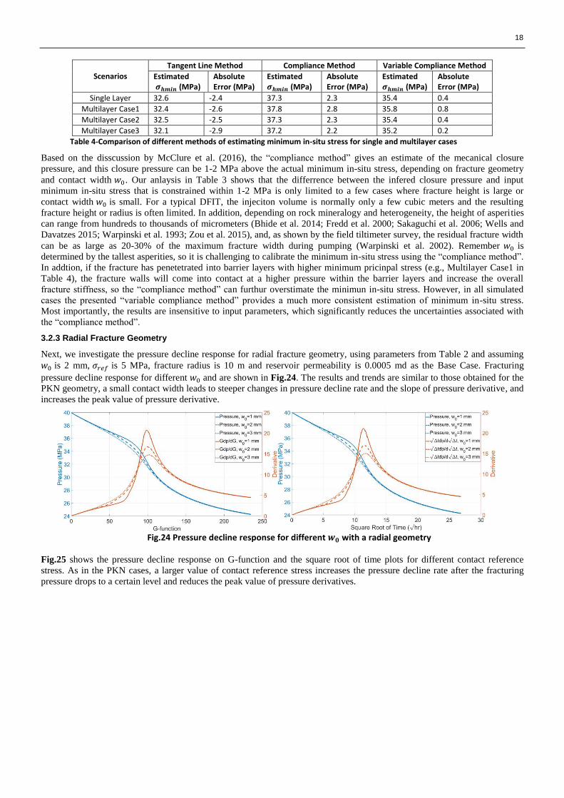
Single Layer 32.6 -2.4 37.3 2.3 35.4 0.4

Multilayer Case1 32.4 -2.6 37.8 2.8 35.8 0.8

Multilayer Case2 32.5 -2.5 37.3 2.3 35.4 0.4

Multilayer Case3 32.1 -2.9 37.2 2.2 35.2 0.2

Table 4-Comparison of different methods of estimating minimum in-situ stress for single and multilayer cases

Based on the disscussion by McClure et al. (2016), the “compliance method” gives an estimate of the mecanical closure

pressure, and this closure pressure can be 1-2 MPa above the actual minimum in-situ stress, depending on fracture geometry

and contact width 𝑤0 . Our anlaysis in Table 3 shows that the differrence between the infered closure pressure and input

minimum in-situ stress that is constrained within 1-2 MPa is only limited to a few cases where fracture height is large or

contact width 𝑤0 is small. For a typical DFIT, the injeciton volume is normally only a few cubic meters and the resulting

fracture height or radius is often limited. In addition, depending on rock mineralogy and heterogeneity, the height of asperities

can range from hundreds to thousands of micrometers (Bhide et al. 2014; Fredd et al. 2000; Sakaguchi et al. 2006; Wells and

Davatzes 2015; Warpinski et al. 1993; Zou et al. 2015), and, as shown by the field tiltimeter survey, the residual fracture width

can be as large as 20-30% of the maximum fracture width during pumping (Warpinski et al. 2002). Remember 𝑤0 is

determined by the tallest asperities, so it is challenging to calibrate the minimum in-situ stress using the “compliance method”.

In addtion, if the fracture has penetetrated into barrier layers with higher minimum pricinpal stress (e.g., Multilayer Case1 in

Table 4), the fracture walls will come into contact at a higher pressure within the barrier layers and increase the overall

fracture stiffness, so the “compliance method” can furthur overstimate the minimun in-situ stress. However, in all simulated

cases the presented “variable compliance method” provides a much more consistent estimation of minimum in-situ stress.

Most importantly, the results are insensitive to input parameters, which significantly reduces the uncertainties associated with

the “compliance method”.

3.2.3 Radial Fracture Geometry

Next, we investigate the pressure decline response for radial fracture geometry, using parameters from Table 2 and assuming

𝑤0 is 2 mm, 𝜎𝑟𝑒𝑓 is 5 MPa, fracture radius is 10 m and reservoir permeability is 0.0005 md as the Base Case. Fracturing

pressure decline response for different 𝑤0 and are shown in Fig.24. The results and trends are similar to those obtained for the

PKN geometry, a small contact width leads to steeper changes in pressure decline rate and the slope of pressure derivative, and

increases the peak value of pressure derivative.

Fig.24 Pressure decline response for different 𝒘𝟎 with a radial geometry

Fig.25 shows the pressure decline response on G-function and the square root of time plots for different contact reference

stress. As in the PKN cases, a larger value of contact reference stress increases the pressure decline rate after the fracturing

pressure drops to a certain level and reduces the peak value of pressure derivatives.

19

Fig.25 Pressure decline response for different 𝛔𝐫𝐞𝐟 with a radial geometry

Fig.26 shows the corresponding pressure decline response on G-function and the square root of time plots. A larger fracture

radius leads to lower fracture stiffness and this, in turn, results in a lower pressure decline rate.

Fig.26 Pressure decline response for different fracture radii with a radial geometry.

Fig.27 shows the fracturing pressure and its derivatives for different reservoir permeability on G-function and the square root

of time plots. As expected, pressure declines more rapidly when the reservoir permeability is large. At early time, the pressure

decline rate increases because an increase in the fracture stiffness dominates changes in leak-off rate. At late time when the

fracture becomes less compliant, the pressure decline rate decreases due to smaller and smaller differences between the

fracture pressure and the initial reservoir pressure. Eventually, the leak-off rate will drop to zero as the fracture pressure

becomes equal to the reservoir pressure.

Fig.27 Pressure decline response for different reservoir permeability with a radial geometry

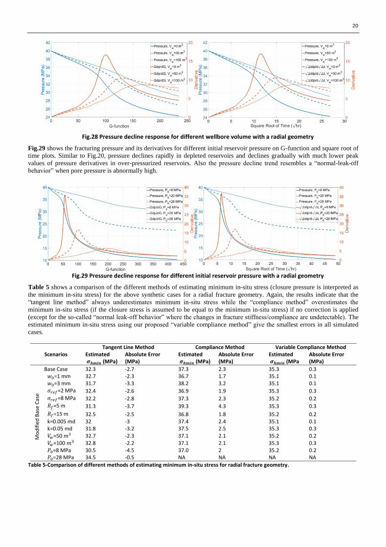
Fig.28 shows the pressure decline response for different wellbore volumes on G-function and the square root of time plots.

Compared to Fig. 19, it can be observed that the WBS effect has stronger influence on pressure decline trend in our radial

fracture geometry for the same wellbore volume. This is because the fracture volume and fracture surface are smaller than that

in previous case of PKN fracture geometry, which intensifies the impact of WBS effect.

20

Fig.28 Pressure decline response for different wellbore volume with a radial geometry

Fig.29 shows the fracturing pressure and its derivatives for different initial reservoir pressure on G-function and square root of

time plots. Similar to Fig.20, pressure declines rapidly in depleted reservoirs and declines gradually with much lower peak

values of pressure derivatives in over-pressurized reservoirs. Also the pressure decline trend resembles a “normal-leak-off

behavior” when pore pressure is abnormally high.

Fig.29 Pressure decline response for different initial reservoir pressure with a radial geometry

Table 5 shows a comparison of the different methods of estimating minimum in-situ stress (closure pressure is interpreted as

the minimum in-situ stress) for the above synthetic cases for a radial fracture geometry. Again, the results indicate that the

“tangent line method” always underestimates minimum in-situ stress while the “compliance method” overestimates the

minimum in-situ stress (if the closure stress is assumed to be equal to the minimum in-situ stress) if no correction is applied

(except for the so-called “normal leak-off behavior” where the changes in fracture stiffness/compliance are undetectable). The

estimated minimum in-situ stress using our proposed “variable compliance method” give the smallest errors in all simulated

cases.

Scenarios Tangent Line Method Compliance Method Variable Compliance Method

Estimated 𝝈𝒉𝒎𝒊𝒏 (MPa)

Absolute Error (MPa)

Estimated 𝝈𝒉𝒎𝒊𝒏 (MPa)

Absolute Error (MPa)

Estimated 𝝈𝒉𝒎𝒊𝒏 (MPa

Absolute Error (MPa)

Base Case 32.3 -2.7 37.3 2.3 35.3 0.3

Mo

dif

ied

Bas

e C

ase

𝑤0=1 mm 32.7 -2.3 36.7 1.7 35.1 0.1 𝑤0=3 mm 31.7 -3.3 38.2 3.2 35.1 0.1 𝜎𝑟𝑒𝑓=2 MPa 32.4 -2.6 36.9 1.9 35.3 0.3 𝜎𝑟𝑒𝑓=8 MPa 32.2 -2.8 37.3 2.3 35.2 0.2 𝑅𝑓=5 m 31.3 -3.7 39.3 4.3 35.3 0.3

𝑅𝑓=15 m 32.5 -2.5 36.8 1.8 35.2 0.2 k=0.005 md 32 -3 37.4 2.4 35.1 0.1 k=0.05 md 31.8 -3.2 37.5 2.5 35.3 0.3 𝑉𝑤=50 𝑚3 32.7 -2.3 37.1 2.1 35.2 0.2 𝑉𝑤=100 𝑚3 32.8 -2.2 37.1 2.1 35.3 0.3 𝑃0=8 MPa 30.5 -4.5 37.0 2 35.2 0.2 𝑃0=28 MPa 34.5 -0.5 NA NA NA NA

Table 5-Comparison of different methods of estimating minimum in-situ stress for radial fracture geometry.

21

From the analysis presented in this section, we can conclude that the pressure decline response during DFIT is affected by

many parameters, such as fracture geometry, reservoir properties, fracture surface roughness, etc. As a result any history match

DFIT data can be non-unique if we don’t have good knowledge (from other independent analysis and measurements) of the

constraints on these parameters. Nevertheless, our proposed “variable compliance method” gives the most reliable estimation

of minimum in-situ stress regardless of these parameters, so the uncertainties associated with fracture geometry, surface

roughness and reservoir properties do not impact our estimation of minimum in-situ stress.

4. Field Data Interpretation

4.1 Field Case 1

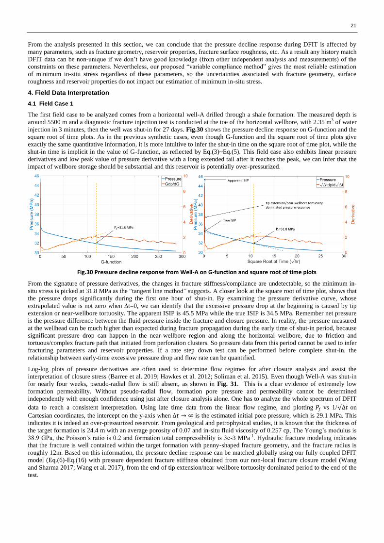
The first field case to be analyzed comes from a horizontal well-A drilled through a shale formation. The measured depth is

around 5500 m and a diagnostic fracture injection test is conducted at the toe of the horizontal wellbore, with 2.35 m3 of water

injection in 3 minutes, then the well was shut-in for 27 days. Fig.30 shows the pressure decline response on G-function and the

square root of time plots. As in the previous synthetic cases, even though G-function and the square root of time plots give

exactly the same quantitative information, it is more intuitive to infer the shut-in time on the square root of time plot, while the

shut-in time is implicit in the value of G-function, as reflected by Eq.(3)~Eq.(5). This field case also exhibits linear pressure

derivatives and low peak value of pressure derivative with a long extended tail after it reaches the peak, we can infer that the

impact of wellbore storage should be substantial and this reservoir is potentially over-pressurized.

Fig.30 Pressure decline response from Well-A on G-function and square root of time plots

From the signature of pressure derivatives, the changes in fracture stiffness/compliance are undetectable, so the minimum in-

situ stress is picked at 31.8 MPa as the “tangent line method” suggests. A closer look at the square root of time plot, shows that

the pressure drops significantly during the first one hour of shut-in. By examining the pressure derivative curve, whose

extrapolated value is not zero when ∆t=0, we can identify that the excessive pressure drop at the beginning is caused by tip

extension or near-wellbore tortuosity. The apparent ISIP is 45.5 MPa while the true ISIP is 34.5 MPa. Remember net pressure

is the pressure difference between the fluid pressure inside the fracture and closure pressure. In reality, the pressure measured

at the wellhead can be much higher than expected during fracture propagation during the early time of shut-in period, because

significant pressure drop can happen in the near-wellbore region and along the horizontal wellbore, due to friction and

tortuous/complex fracture path that initiated from perforation clusters. So pressure data from this period cannot be used to infer

fracturing parameters and reservoir properties. If a rate step down test can be performed before complete shut-in, the

relationship between early-time excessive pressure drop and flow rate can be quantified.

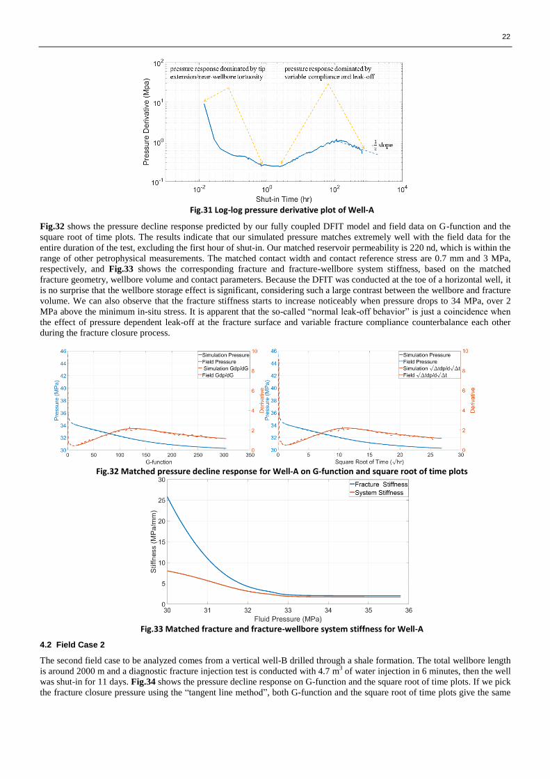
Log-log plots of pressure derivatives are often used to determine flow regimes for after closure analysis and assist the

interpretation of closure stress (Barree et al. 2019; Hawkes et al. 2012; Soliman et al. 2015). Even though Well-A was shut-in

for nearly four weeks, pseudo-radial flow is still absent, as shown in Fig. 31. This is a clear evidence of extremely low

formation permeability. Without pseudo-radial flow, formation pore pressure and permeability cannot be determined

independently with enough confidence using just after closure analysis alone. One has to analyze the whole spectrum of DFIT

data to reach a consistent interpretation. Using late time data from the linear flow regime, and plotting 𝑃𝑓 vs 1/√∆𝑡 on

Cartesian coordinates, the intercept on the y-axis when ∆𝑡 → ∞ is the estimated initial pore pressure, which is 29.1 MPa. This

indicates it is indeed an over-pressurized reservoir. From geological and petrophysical studies, it is known that the thickness of

the target formation is 24.4 m with an average porosity of 0.07 and in-situ fluid viscosity of 0.257 cp, The Young’s modulus is

38.9 GPa, the Poisson’s ratio is 0.2 and formation total compressibility is 3e-3 MPa-1

. Hydraulic fracture modeling indicates

that the fracture is well contained within the target formation with penny-shaped fracture geometry, and the fracture radius is

roughly 12m. Based on this information, the pressure decline response can be matched globally using our fully coupled DFIT

model (Eq.(6)-Eq.(16) with pressure dependent fracture stiffness obtained from our non-local fracture closure model (Wang

and Sharma 2017; Wang et al. 2017), from the end of tip extension/near-wellbore tortuosity dominated period to the end of the

test.

22

Fig.31 Log-log pressure derivative plot of Well-A

Fig.32 shows the pressure decline response predicted by our fully coupled DFIT model and field data on G-function and the

square root of time plots. The results indicate that our simulated pressure matches extremely well with the field data for the

entire duration of the test, excluding the first hour of shut-in. Our matched reservoir permeability is 220 nd, which is within the

range of other petrophysical measurements. The matched contact width and contact reference stress are 0.7 mm and 3 MPa,

respectively, and Fig.33 shows the corresponding fracture and fracture-wellbore system stiffness, based on the matched

fracture geometry, wellbore volume and contact parameters. Because the DFIT was conducted at the toe of a horizontal well, it

is no surprise that the wellbore storage effect is significant, considering such a large contrast between the wellbore and fracture

volume. We can also observe that the fracture stiffness starts to increase noticeably when pressure drops to 34 MPa, over 2

MPa above the minimum in-situ stress. It is apparent that the so-called “normal leak-off behavior” is just a coincidence when

the effect of pressure dependent leak-off at the fracture surface and variable fracture compliance counterbalance each other

during the fracture closure process.

Fig.32 Matched pressure decline response for Well-A on G-function and square root of time plots

Fig.33 Matched fracture and fracture-wellbore system stiffness for Well-A

4.2 Field Case 2

The second field case to be analyzed comes from a vertical well-B drilled through a shale formation. The total wellbore length

is around 2000 m and a diagnostic fracture injection test is conducted with 4.7 m3 of water injection in 6 minutes, then the well

was shut-in for 11 days. Fig.34 shows the pressure decline response on G-function and the square root of time plots. If we pick

the fracture closure pressure using the “tangent line method”, both G-function and the square root of time plots give the same

23

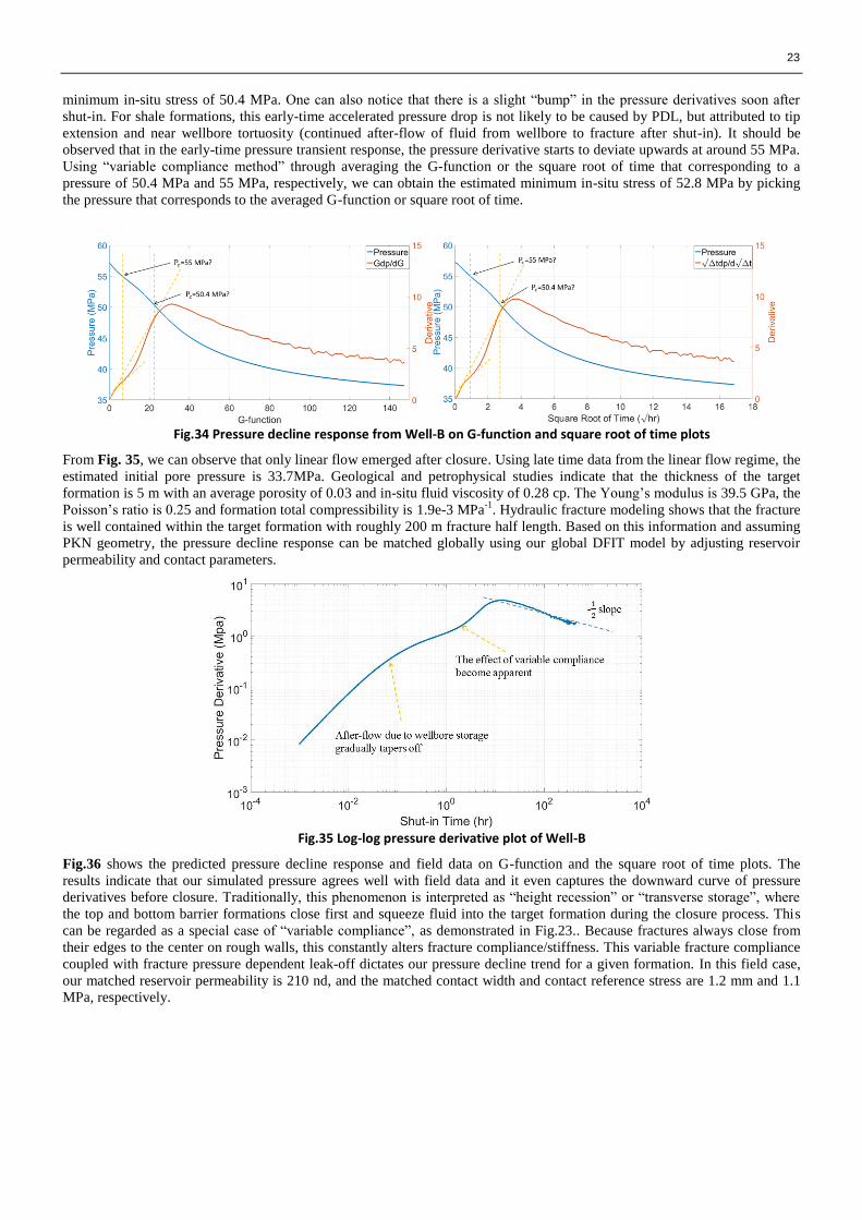
minimum in-situ stress of 50.4 MPa. One can also notice that there is a slight “bump” in the pressure derivatives soon after

shut-in. For shale formations, this early-time accelerated pressure drop is not likely to be caused by PDL, but attributed to tip

extension and near wellbore tortuosity (continued after-flow of fluid from wellbore to fracture after shut-in). It should be

observed that in the early-time pressure transient response, the pressure derivative starts to deviate upwards at around 55 MPa.

Using “variable compliance method” through averaging the G-function or the square root of time that corresponding to a

pressure of 50.4 MPa and 55 MPa, respectively, we can obtain the estimated minimum in-situ stress of 52.8 MPa by picking

the pressure that corresponds to the averaged G-function or square root of time.

Fig.34 Pressure decline response from Well-B on G-function and square root of time plots

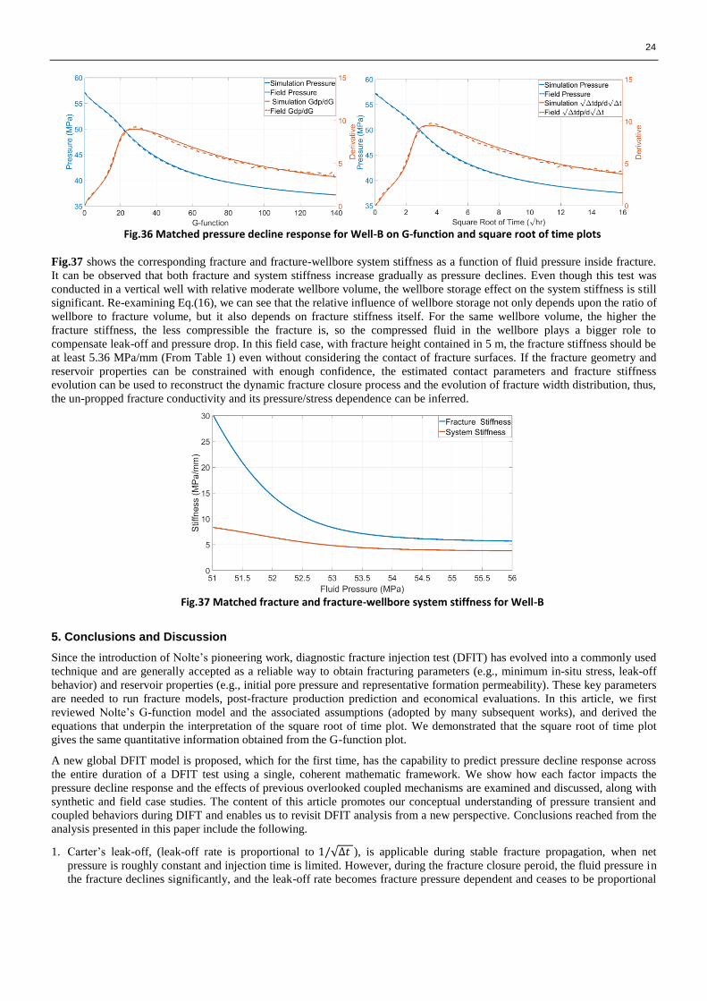
From Fig. 35, we can observe that only linear flow emerged after closure. Using late time data from the linear flow regime, the

estimated initial pore pressure is 33.7MPa. Geological and petrophysical studies indicate that the thickness of the target

formation is 5 m with an average porosity of 0.03 and in-situ fluid viscosity of 0.28 cp. The Young’s modulus is 39.5 GPa, the

Poisson’s ratio is 0.25 and formation total compressibility is 1.9e-3 MPa-1

. Hydraulic fracture modeling shows that the fracture

is well contained within the target formation with roughly 200 m fracture half length. Based on this information and assuming

PKN geometry, the pressure decline response can be matched globally using our global DFIT model by adjusting reservoir

permeability and contact parameters.

Fig.35 Log-log pressure derivative plot of Well-B

Fig.36 shows the predicted pressure decline response and field data on G-function and the square root of time plots. The

results indicate that our simulated pressure agrees well with field data and it even captures the downward curve of pressure

derivatives before closure. Traditionally, this phenomenon is interpreted as “height recession” or “transverse storage”, where

the top and bottom barrier formations close first and squeeze fluid into the target formation during the closure process. This

can be regarded as a special case of “variable compliance”, as demonstrated in Fig.23.. Because fractures always close from

their edges to the center on rough walls, this constantly alters fracture compliance/stiffness. This variable fracture compliance

coupled with fracture pressure dependent leak-off dictates our pressure decline trend for a given formation. In this field case,

our matched reservoir permeability is 210 nd, and the matched contact width and contact reference stress are 1.2 mm and 1.1

MPa, respectively.

24

Fig.36 Matched pressure decline response for Well-B on G-function and square root of time plots

Fig.37 shows the corresponding fracture and fracture-wellbore system stiffness as a function of fluid pressure inside fracture.

It can be observed that both fracture and system stiffness increase gradually as pressure declines. Even though this test was

conducted in a vertical well with relative moderate wellbore volume, the wellbore storage effect on the system stiffness is still

significant. Re-examining Eq.(16), we can see that the relative influence of wellbore storage not only depends upon the ratio of

wellbore to fracture volume, but it also depends on fracture stiffness itself. For the same wellbore volume, the higher the

fracture stiffness, the less compressible the fracture is, so the compressed fluid in the wellbore plays a bigger role to

compensate leak-off and pressure drop. In this field case, with fracture height contained in 5 m, the fracture stiffness should be

at least 5.36 MPa/mm (From Table 1) even without considering the contact of fracture surfaces. If the fracture geometry and

reservoir properties can be constrained with enough confidence, the estimated contact parameters and fracture stiffness

evolution can be used to reconstruct the dynamic fracture closure process and the evolution of fracture width distribution, thus,

the un-propped fracture conductivity and its pressure/stress dependence can be inferred.

Fig.37 Matched fracture and fracture-wellbore system stiffness for Well-B

5. Conclusions and Discussion

Since the introduction of Nolte’s pioneering work, diagnostic fracture injection test (DFIT) has evolved into a commonly used

technique and are generally accepted as a reliable way to obtain fracturing parameters (e.g., minimum in-situ stress, leak-off

behavior) and reservoir properties (e.g., initial pore pressure and representative formation permeability). These key parameters

are needed to run fracture models, post-fracture production prediction and economical evaluations. In this article, we first

reviewed Nolte’s G-function model and the associated assumptions (adopted by many subsequent works), and derived the

equations that underpin the interpretation of the square root of time plot. We demonstrated that the square root of time plot

gives the same quantitative information obtained from the G-function plot.

A new global DFIT model is proposed, which for the first time, has the capability to predict pressure decline response across

the entire duration of a DFIT test using a single, coherent mathematic framework. We show how each factor impacts the

pressure decline response and the effects of previous overlooked coupled mechanisms are examined and discussed, along with

synthetic and field case studies. The content of this article promotes our conceptual understanding of pressure transient and

coupled behaviors during DIFT and enables us to revisit DFIT analysis from a new perspective. Conclusions reached from the

analysis presented in this paper include the following.

1. Carter’s leak-off, (leak-off rate is proportional to 1/√∆𝑡 ), is applicable during stable fracture propagation, when net

pressure is roughly constant and injection time is limited. However, during the fracture closure peroid, the fluid pressure in

the fracture declines significantly, and the leak-off rate becomes fracture pressure dependent and ceases to be proportional

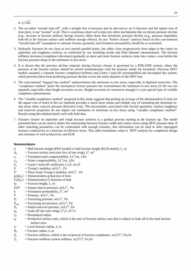
25

to 1/√∆𝑡 .

2. The so-called “normal leak-off”, with a straight line of pressure and its derivatives on G-function and the square root of

time plots, is not “normal” at all. This is sometimes observed in data sets when mechanisms that accelerate pressure decline

(e.g., increase in fracture stiffness during closure) offset those that decelerate pressure decline (e.g., pressure dependent

leak-off at the fracture surface and wellbore storage effects). So any “before closure” analysis based on this conventional

“normal leak-off” assumption to estimate fracture geometry and formation permeability should be re-examined.

3. Hydraulic fractures do not close as two smooth parallel plates, but rather close progressively from edges to the center on

asperities and roughness surfaces, as confirmed by our modeling results and field tiltmeter measurements. The fracture

stiffness increases (compliance decreases) gradually as more and more fracture surfaces come into contact, even before the

fracture pressure drops to the minimum in-situ stress.

4. It is shown that the pressure decline response during fracture closure is governed by a PDE-ODE system, where the

pressure at the fracture surface should be solved simultaneously with the pressure inside the formation. Previous DFIT

models assumed a constant fracture compliance/stiffness and Carter’s leak-off oversimplified and decoupled this system,

which prevents them from predicting pressure decline across the entire duration of the DFIT test.

5. The conventional “tangent line method” underestimates the minimum in-situ stress, especially in depleted reservoirs. The

“compliance method” picks the mechanical closure pressure but overestimates the minimum in-situ stress (if the two are

equated), especially when height recession occurs. Height recession (or transverse storage) is a just special type of variable

compliance phenomenon.

6. The “variable compliance method” proposed in this study suggests that picking an average of the dimensionless G-time (or

the square root of time) of the two methods provides a much more robust and reliable way of estimating the minimum in-

situ stress when concave pressure derivative exist. The uncertainties associated with fracture geometry, surface roughness

and reservoir properties do not impact our estimation of minimum in-situ stress using “variable compliance method”.

Results using this method match well with field data.

7. Fracture closure on asperities and rough fracture surfaces is a gradual process starting at the fracture tip. The model

presented here can be used to define the relationship between fracture width and contact stress using DFIT pressure data. If

other matching parameters can be constrained with enough certainty, this information can be used to infer unpropped

fracture conductivity as a function of effective stress. This adds tremendous value to DFIT analysis for completion design

and estimates of well productivity and EUR.

Nomenclature

𝑎

= Half fracture height (PKN model) or half fracture length (KGD model), L, 𝑚

𝐴𝑓

= Fracture surface area (one face of one wing), 𝐿2, 𝑚2

𝑐𝑡

= Formation total compressibility, L𝑡2/𝑚, 1/Pa

𝑐𝑤

= Water compressibility, L𝑡2/𝑚, 1/Pa

𝐶𝐿

= Carter’s leak-off coefficient, L/√𝑡, m/√𝑠

𝐸

= Young’s modulus, m/L𝑡2, 𝑃𝑎

𝐸′

= Plane strain Young’s modulus, m/L𝑡2, 𝑃𝑎

𝑔(∆𝑡𝐷) = Dimensionless g-function of time

𝐺(∆𝑡𝐷) = Dimensionless G-function of time

ℎ𝑓

= Fracture height, L, 𝑚

𝐼𝑆𝐼𝑃

= Instant shut-in pressure, m/L𝑡2, 𝑃𝑎

𝑘

= Formation permeability, 𝐿2, 𝑚2

𝑃

= Pressure, m/L𝑡2, 𝑃𝑎

𝑃𝑓

= Fracturing pressure, m/L𝑡2, 𝑃𝑎

𝑃𝑛𝑒𝑡

= Fracturing net pressure, m/L𝑡2, 𝑃𝑎

𝑃0

= Initial reservoir pressure, m/L𝑡2, 𝑃𝑎

𝑞𝑓

= Leak-off rate (one wing), 𝐿3/𝑡, 𝑚3/𝑠

𝑟𝐷

= Normalized radius

𝑟𝑝

= Productive surface ratio, which is the ratio of fracture surface area that is subject to leak-off to the total fracture

surface area.

𝑟𝑓

= Local fracture radius, 𝐿, 𝑚

𝑅𝑓

= Fracture radius, 𝐿, 𝑚

𝑆𝑓

= Fracture stiffness, which is the reciprocal of fracture compliance, 𝑚/𝐿2𝑡2, 𝑃𝑎/𝑚

𝑆𝑠

= Fracture-wellbore system stiffness, 𝑚/𝐿2𝑡2, 𝑃𝑎/𝑚

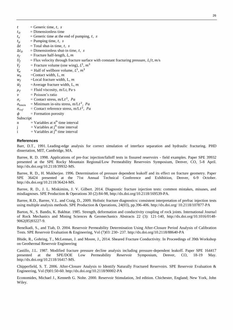
26

𝑡

= Generic time, 𝑡, 𝑠

𝑡𝐷

= Dimensionless time

𝑡𝑒

= Generic time at the end of pumping, 𝑡, 𝑠

𝑡𝑝

= Pumping time, 𝑡, 𝑠

∆𝑡

= Total shut-in time, 𝑡, 𝑠

∆𝑡𝐷

= Dimensionless shut-in time, 𝑡, 𝑠

𝑥𝑓

= Fracture half-length, 𝐿, 𝑚

𝑈𝑓

= Flux velocity through fracture surface with constant fracturing pressure, 𝐿/𝑡, 𝑚/s

𝑉𝑓

= Fracture volume (one wing), 𝐿3, 𝑚3

𝑉𝑤

= Half of wellbore volume, 𝐿3, 𝑚3

𝑤0

=Contact width, L, 𝑚

𝑤𝑓

=Local fracture width, L, 𝑚

�̅�𝑓

=Average fracture width, L, 𝑚

𝜇𝑓

= Fluid viscosity, m/Lt, Pa·s

𝜈

= Poisson’s ratio

𝜎𝑐

= Contact stress, m/L𝑡2, 𝑃𝑎

𝜎ℎ𝑚𝑖𝑛

= Minimum in-situ stress, m/L𝑡2, 𝑃𝑎

𝜎𝑟𝑒𝑓

= Contact reference stress, m/L𝑡2, 𝑃𝑎

𝜙

= Formation porosity

Subscript

n = Variables at nth

time interval

j = Variables at jth

time interval

i = Variables at jth

time interval

References

Barr, D.T., 1991. Leading-edge analysis for correct simulation of interface separation and hydraulic fracturing. PHD

dissertation, MIT, Cambridge, MA.

Barree, R. D. 1998. Applications of pre-frac injection/falloff tests in fissured reservoirs - field examples. Paper SPE 39932

presented at the SPE Rocky Mountain Regional/Low Permeability Reservoirs Symposium, Denver, CO, 5-8 April.

http://dx.doi.org/10.2118/39932-MS.

Barree, R. D., H. Mukherjee. 1996. Determination of pressure dependent leakoff and its effect on fracture geometry. Paper

SPE 36424 presented at the 71st Annual Technical Conference and Exhibition, Denver, 6-9 October.

http://dx.doi.org/10.2118/36424-MS.

Barree, R. D., J. L. Miskimins, J. V. Gilbert. 2014. Diagnostic fracture injection tests: common mistakes, misuses, and

misdiagnoses. SPE Production & Operations 30 (2):84-98, http://dx.doi.org/10.2118/169539-PA.

Barree, R.D., Barree, V.L. and Craig, D., 2009. Holistic fracture diagnostics: consistent interpretation of prefrac injection tests

using multiple analysis methods. SPE Production & Operations, 24(03), pp.396-406. http://dx.doi.org/ 10.2118/107877-PA

Barton, N., S. Bandis, K. Bakhtar. 1985. Strength, deformation and conductivity coupling of rock joints. International Journal

of Rock Mechanics and Mining Sciences & Geomechanics Abstracts 22 (3): 121-140, http://dx.doi.org/10.1016/0148-

9062(85)93227-9.

Benelkadi, S., and Tiab, D. 2004. Reservoir Permeability Determination Using After-Closure Period Analysis of Calibration

Tests. SPE Reservoir Evaluation & Engineering, Vol (7)03: 230- 237. http://dx.doi.org/10.2118/88640-PA

Bhide, R., Gohring, T., McLennan, J. and Moore, J., 2014. Sheared Fracture Conductivity. In Proceedings of 39th Workshop

on Geothermal Reservoir Engineering

Castillo, J.L. 1987. Modified fracture pressure decline analysis including pressure-dependent leakoff. Paper SPE 164417

presented at the SPE/DOE Low Permeability Reservoir Symposium, Denver, CO, 18-19 May.

http://dx.doi.org/10.2118/16417-MS.

Chipperfield, S. T. 2006. After-Closure Analysis to Identify Naturally Fractured Reservoirs. SPE Reservoir Evaluation &

Engineering, Vol (9)01:50-60. http://dx.doi.org/10.2118/90002-PA

Economides, Michael J., Kenneth G. Nolte. 2000. Reservoir Stimulation, 3rd edition. Chichester, England; New York, John

Wiley.

27

England, A.H. and Green, A.E., 1963, April. Some two-dimensional punch and crack problems in classical elasticity. In Proc.

Camb. Phil. Soc (Vol. 59, No. 2, p. 489). http://www.doi.org/10.1017/S0305004100037099

Fredd, C. N., McConnell, S. B., Boney, C. L., & England, K. W. 2000. Experimental Study of Hydraulic Fracture

Conductivity Demonstrates the Benefits of Using Proppants. Paper SPE 60326 presented at the

SPE Rocky Mountain Regional/Low-Permeability Reservoirs Symposium and Exhibition, Denver, Colorado, 12-15 March.

http://dx.doi.org/10.2118/60326-MS

Fu, Y., Dehghanpour, H., Ezulike, D. O., and Jones, R. S. 2017. Estimating Effective Fracture Pore Volume From Flowback

Data and Evaluating Its Relationship to Design Parameters of Multistage-Fracture Completion. SPE Production & Operations

(PrePrint). https://doi.org/10.2118/175892-PA

Gringarten, A. C., Ramey, H. J., and Raghavan, R. 1974. Unsteady-State Pressure Distributions Created by a Well with a

Single Infinite-Conductivity Vertical Fracture. SPE Journal. Vol(14)04:347-360. http://dx.doi.org/10.2118/4051-PA

Hawkes, R., Bachman, R. C., Walters, D. A., Toussaint, F. L., and Settari, T. 2012. Reappraisal of the G Time Concept in

Mini-Frac Analysis. Paper SPE 160169 presented at the SPE Annual Technical Conference and Exhibition, San Antonio,

Texas, USA, 8-10 October. https://dx.doi.org/10.2118/160169-MS

Koning, E.J.L. and Niko, H., 1985, January. Fractured Water-Injection Wells: A Pressure Falloff Test for Determining

Fracture Dimensions. Paper SPE 14458 presented at the SPE Annual Technical Conference and Exhibition, Las Vegas,

Nevada, 22-26 September. https://doi.org/10.2118/14458-MS

Liu, G., Ehlig-Economides, C. and Sun, J. 2016. Comprehensive Global Fracture Calibration Model. Paper SPE 181856

presented at the SPE Asia Pacific Hydraulic Fracturing Conference, Beijing, China, August 24-26.

http://dx.doi.org/10.2118/181856-MS

Loughry, D., Epps, D. and Forrest, J., 2015. Using Pad ISIP, DFIT, and ESP Data to Generate a Pore Pressure Model for the

Midland Basin. Paper presented at the Unconventional Resources Technology Conference, San Antonio, Texas, USA, 20-22

July. https://doi.org/10.15530/URTEC-2015-2162973

Marongiu-Porcu, Matteo, Albertus Retnanto, Michael J. Economides, Christine Ehlig-Economides. 2014. Comprehensive

fracture calibration test design. Paper SPE 168634 presented at the SPE Hydraulic Fracturing Technology Conference, The

Woodlands, TX, February 4-6. http://dx.doi.org/10.2118/168634-MS

Mayerhofer, M. J., and Economides, M. J. 1997. Fracture-Injection-Test Interpretation: Leakoff Coefficient vs. Permeability.

SPE Production & Facilities. Vol (12) 04:231-236. http://dx.doi.org/10.2118/28562-PA

Mayerhofer, M. J., Ehlig-Economides, C. A., and Economides, M. J. 1995. Pressure Transient Analysis of Fracture

Calibration Tests. Journal of Petroleum Technology. Vol(47)03:229-234. http://dx.doi.org/10.2118/26527-PA

McClure, M.W. 2017. The Spurious Deflection on Log-Log Superposition Time Derivative Plots of Diagnostic Fracture. SPE

Reservoir Evaluation & Engineering (In Press). https://doi.org/10.2118/186098-PA

McClure, M.W., Jung, H., Cramer, D.D. and Sharma, M.M., 2016. The Fracture Compliance Method for Picking Closure

Pressure from Diagnostic Fracture-Injection Tests. SPE Journal 21(04):1321-1339. http://dx.doi.org/10.2118/179725-PA

Mirani, A., Marongiu-Porcu, M., Wang, H., and Philippe, E. Production Pressure Drawdown Management for Fractured

Horizontal Wells in Shale Gas Formations. 2016. Paper SPE 181365 presented at the SPE Annual Technical Conference and

Exhibition held in Dubai, UAE, 26-28 Sep. http://dx.doi.org/10.2118/181365-MS

Nolte, K. G. 1979. Determination of Fracture Parameters from Fracturing Pressure Decline. Paper 8341 presented at the SPE

Annual Technical Conference and Exhibition, Las Vegas, Nevada, 23-26 September. http://dx.doi.org/10.2118/8341-MS

Nolte, K. G. 1986. A General Analysis of Fracturing Pressure Decline with Application to Three Models. SPE Formation

Evaluation. Vol (1) 06:571-583. http://dx.doi.org/10.2118/12941-PA

Nolte, K. G., Maniere, J. L., and Owens, K. A. 1997. After-Closure Analysis of Fracture Calibration Tests. Paper SPE 38676

presented at the SPE Annual Technical Conference and Exhibition, San Antonio, Texas, 5-8 October.

http://dx.doi.org/10.2118/38676-MS

Potocki, D. J. 2012. Understanding Induced Fracture Complexity in Different Geological Settings Using DFIT Net Fracture

Pressure. Paper SPE 162814 presented at the SPE Canadian Unconventional Resources Conference, Calgary, Alberta, Canada,

30 October-1 November. http://dx.doi.org/10.2118/162814-MS

Ramurthy, M., Barree, R.D., Kundert, D.P., Petre, J.E. and Mullen, M.J., 2011. Surface-area vs. conductivity-type fracture

treatments in shale reservoirs. SPE Production & Pperations, 26(04), pp.357-367. https://doi.org/10.2118/140169-PA

28

Sakaguchi, K., Tomono, J., Okumura, K., Ogawa, Y. and Matsuki, K., 2008. Asperity height and aperture of an artificial

tensile fracture of metric size. Rock Mechanics and Rock Engineering, 41(2), pp.325-341. http://dx.doi.org/ 10.1007/s00603-

005-0102-3

Schiesser, W.E. and Griffiths, G.W., 2009. A compendium of partial differential equation models: method of lines analysis

with Matlab. Cambridge University Press.

Sneddon, I. N. and Lowengrub, M., Crack Problems in the Classical Theory of Elasticity. John Wiley & Sons, Inc., New

York, 1969

Soliman, M. Y., Craig, D. P., Bartko, K. M., Rahim, Z., and Adams, D. M. 2005. Post-Closure Analysis to Determine

Formation Permeability, Reservoir Pressure, Residual Fracture Properties. Paper SPE 93419 presented at the SPE Middle East

Oil and Gas Show and Conference, Kingdom of Bahrain,12-15 March. http://dx.doi.org/10.2118/93419-MS

Soliman, M. Y., Shahri, M., and Lamei, H. 2013. Revisiting the Before Closure Analysis Formulations in Diagnostic

Fracturing Injection Test. Paper SPE 163869 presented at the SPE Hydraulic Fracturing Technology Conference, The

Woodlands, Texas, USA, 4-6 February. http://dx.doi.org/10.2118/163869-MS

Soliman, M.Y., Miranda, C., and Wang, H.M. 2010. Application of After-Closure Analysis to a Dual-Porosity Formation, to

CBM, and to a Fractured Horizontal Well. SPE Prod & Oper 25 (4): 472–483. SPE-124135-PA.

http://dx.doi.org/10.2118/124135-PA.

Valko ,́ P. P., and Economides, M. J. 1999. Fluid-Leakoff Delineation in High-Permeability Fracturing. SPE Production &

Facilities. Vol (14)02:110-116. http://dx.doi.org/10.2118/56135-PA

van Dam, D.B., de Pater, C.J. and Romijn, R., 2000. Analysis of Hydraulic Fracture Closure in Laboratory Experiments. SPE

Production & Facilities,15(03), pp.151-158. http://dx.doi.org/10.2118/65066-PA

Wang, H. 2015. Numerical Modeling of Non-Planar Hydraulic Fracture Propagation in Brittle and Ductile Rocks using XFEM

with Cohesive Zone Method. Journal of Petroleum Science and Engineering, Vol (135):127-140.

http://dx.doi.org/10.1016/j.petrol.2015.08.010

Wang, H. 2016. Numerical Investigation of Fracture Spacing and Sequencing Effects on Multiple Hydraulic Fracture

Interference and Coalescence in Brittle and Ductile Reservoir Rocks. Engineering Fracture Mechanics, Vol (157): 107-124.

http://dx.doi.org/10.1016/j.engfracmech.2016.02.025

Wang, H. 2017. What Factors Control Shale Gas Production and Production Decline Trend in Fractured Systems: A

Comprehensive Analysis and Investigation. SPE Journal, Vol 22(02): 562-581. http://dx.doi.org/10.2118/179967-PA

Wang, H. and Sharma, M.M. 2017. A Non-Local Model for Fracture Closure on Rough Fracture Faces and Asperities. Journal

of Petroleum Science and Engineering, 154, 425-437. https://dx.doi.org/10.1016/j.petrol.2017.04.024

Wang, H., Marongiu-Porcu, M., and Economides, M. J. 2016. SPE-168600-PA. Poroelastic and Poroplastic Modeling of

Hydraulic Fracturing in Brittle and Ductile Formations, Journal of SPE Production & Operations, 31(01): 47–59.

http://dx.doi.org/10.2118/168600-PA

Wang, H., Yi,S., and Sharma, M. M. 2017. A Computational efficient method for Solving Crack Closure and Contact

Problems Using Superposition Method. Theoretical and Applied Fracture Mechanics (In Press)

Warpinski, N.R., Branagan, P.T., Engler, B.P., Wilmer,R., and Wolhart, S.L. 2002. Evaluation of a downhole tiltmeter array

for monitoring hydraulic fractures. International Journal of Rock Mechanics and Mining Sciences, Vol (34)3-4: 329.e1–

329.e13. http://dx.doi.org/ 10.1016/S1365-1609(97)00074-9

Warpinski, N.R., Lorenz, J.C., Branagan, P.T., Myal, F.R. and Gall, B.L., 1993. Examination of a Cored Hydraulic Fracture in

a Deep Gas Well (includes associated papers 26302 and 26946). SPE Production & Facilities, 8(03), pp.150-158.

http://dx.doi.org/10.2118/22876-PA

Wells, O.L. and Davatzes N.C., 2015. The History of Dilation Across Natural Fractures Due to Evolving Surface Roughness.

In Proc. 40th Workshop on Geothermal Reservoir Engineering

Willis-Richards, J., K. Watanabe, H. Takahashi. 1996. Progress toward a stochastic rock mechanics model of engineered

geothermal systems. Journal of Geophysical Research 101 (B8): 17481-17496, http://dx.doi.org/10.1029/96JB00882.

Wu, W. and Sharma, M.M., 2017. Acid Fracturing in Shales: Effect of Dilute Acid on Properties and Pore Structure of

Shale. SPE Production & Operations, 32(01):51-63. http://dx.doi.org/10.2118/173390-PA

Zanganeh, B., Clarkson, C.R. and Hawkes, R.V., 2017. Reinterpretation of Fracture Closure Dynamics During Diagnostic

Fracture Injection Tests. Paper SPE 185649 presented at the SPE Western Regional Meeting, Bakersfield, California, 23-27

April. https://doi.org/10.2118/185649-MS

29

Zhang, J., Kamenov, A., Hill, A.D. and Zhu, D., 2014. Laboratory Measurement of Hydraulic-Fracture Conductivities in the

Barnett Shale. SPE Production & Operations, 29(03), pp.216-227. http://dx.doi.org/10.2118/163839-PA

Zou, Y., Ma, X., Zhang, S., Zhou, T., Ehlig-Economides, C. and Li, H., 2015. The Origins of Low‐Fracture Conductivity in

Soft Shale Formations: An Experimental Study. Energy Technology, 3(12), pp.1233-1242.

https://dx.doi.org/10.1002/ente.20150018

Appendix : Solutions of Pressure Decline under Fracture Pressure Dependent Leak-off

In order to overcome the limitations of Nolte’s G-function model and circumvent the use of a constant leak-off coefficient,

Mayerhofer et al. (1995) presented a model that describes unsteady-state fluid flow from fractures of varying area into the

formation, with the filter cake considered as a time and rate dependent skin effect, allowing for superposition of the injection

history, filter cake deposition and associated rate convolution. Valko ́ and Economides (1999) simplified Mayerhofer et al.

(1995) model by assuming constant leak-off rate during fracture propagation and constant fracture area during closure. A

special before closure analysis (BCA) plot with a straight line can be constructed to determine reservoir permeability and

fracture face resistance, without acquiring the initial guess of permeability and fracture area. However, the process to generate

the special BCA plot and predict fall-off pressure is complicated and cumbersome, prone to mistakes that can lead to

dimension inconsistency (Soliman et al. 2013). In addition, their approach used a constant-rate solution of an infinite-

conductivity well introduced by Gringarten et al. (1974). The results obtained by use of the constant-rate solution are

questionable to account for the fracture pressure dependent leak-off behavior. In this appendix, we derive the solutions of

pressure decline under fracture pressure dependent leak-off using superposition based on constant-pressure solution.

The basic principle of superposition is that the response of a system to a number of perturbations is equal to the sum of the

responses to each of the perturbation as if they were present by themselves if the responses are linearly related to the

perturbations. From Eq.(18), we can calculate the leak-off rate under a constant fracture pressure Pf:

𝑞𝑓 = 2𝐴𝑓(𝑃𝑓 − 𝑃0)√𝑘𝜙𝑐𝑡

𝜋𝜇𝑓∆𝑡 (A. 1)

Divide the shut-in time ∆t into n time steps, and the leak-off rate at the nth

time step can be determined based on superposition:

𝑞𝑓,𝑛 = 2𝐴𝑓√𝑘𝜙𝑐𝑡

𝜋𝜇𝑓

∑𝑃𝑓,𝑗 − 𝑃𝑓,𝑗−1

√∆𝑡𝑛 − ∆𝑡𝑗−1

𝑛

𝑗=1

(A. 2)

The pressure difference Pf,j − Pf,j−1 is the pressure in the fracture at time step j minus the pressure in the formation at the

fracture-formation interface, which equals to the pressure in the fracture at the previous time step. Combine Eq.(A.2) with

Eq.(10) via material balance, we can get:

− 1

𝑆𝑓

𝑑𝑃𝑓,𝑛

𝑑∆𝑡𝑛

= 2√𝑘𝜙𝑐𝑡

𝜋𝜇𝑓

∑𝑃𝑓,𝑗 − 𝑃𝑓,𝑗−1

√∆𝑡𝑛 − ∆𝑡𝑗−1

𝑛

𝑗=1

(A. 3)

let 𝑃𝑓,0 = 𝑃0, 𝑃𝑓,1 = ISIP, ∆𝑡1 = 0, then for 𝑛 ≥ 2, integrate Eq.(A.3) we can obtain :

𝑃𝑓,𝑛 = ISIP − 4𝑆𝑓√𝑘𝜙𝑐𝑡

𝜋𝜇𝑓

∑ ∑(𝑃𝑓,𝑗 − 𝑃𝑓,𝑗−1)(√∆𝑡𝑛 − ∆𝑡𝑗−1

𝑛−1

𝑗=1

𝑛−1

𝑛=1

− √∆𝑡𝑛−1 − ∆𝑡𝑗−1 ) (A. 4)

Eq.(A.4) can be solved explicitly with marching time interval, for example, when 𝑛 = 2

Pf(∆t2) = ISIP − 4Sf(ISIP − P0)√kϕct∆t2

πμf

(A. 5)

On closer observation of Eq.(A.5), we can realize that it is exactly Carter’s leak-off solution to Eq.(19), because during the

first time step, no superposition is needed. The fracture pressure dependent leak-off coefficient can be recovered as:

𝐶𝐿 = (𝑃𝑓 − 𝑃0)√𝑘𝜙𝑐𝑡

𝜋𝜇𝑓

(A. 6)

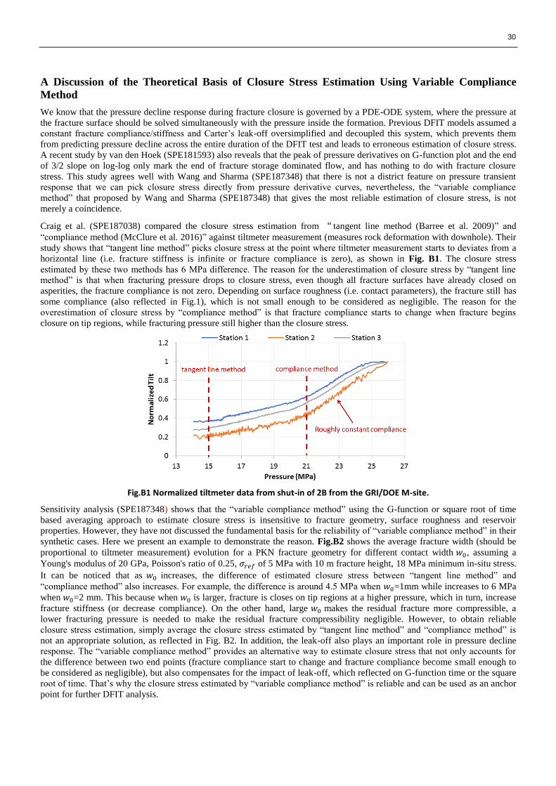
30

A Discussion of the Theoretical Basis of Closure Stress Estimation Using Variable Compliance

Method

We know that the pressure decline response during fracture closure is governed by a PDE-ODE system, where the pressure at

the fracture surface should be solved simultaneously with the pressure inside the formation. Previous DFIT models assumed a

constant fracture compliance/stiffness and Carter’s leak-off oversimplified and decoupled this system, which prevents them

from predicting pressure decline across the entire duration of the DFIT test and leads to erroneous estimation of closure stress.

A recent study by van den Hoek (SPE181593) also reveals that the peak of pressure derivatives on G-function plot and the end

of 3/2 slope on log-log only mark the end of fracture storage dominated flow, and has nothing to do with fracture closure

stress. This study agrees well with Wang and Sharma (SPE187348) that there is not a district feature on pressure transient

response that we can pick closure stress directly from pressure derivative curves, nevertheless, the “variable compliance

method” that proposed by Wang and Sharma (SPE187348) that gives the most reliable estimation of closure stress, is not

merely a coincidence.

Craig et al. (SPE187038) compared the closure stress estimation from “tangent line method (Barree et al. 2009)” and

“compliance method (McClure et al. 2016)” against tiltmeter measurement (measures rock deformation with downhole). Their

study shows that “tangent line method” picks closure stress at the point where tiltmeter measurement starts to deviates from a

horizontal line (i.e. fracture stiffness is infinite or fracture compliance is zero), as shown in Fig. B1. The closure stress

estimated by these two methods has 6 MPa difference. The reason for the underestimation of closure stress by “tangent line

method” is that when fracturing pressure drops to closure stress, even though all fracture surfaces have already closed on

asperities, the fracture compliance is not zero. Depending on surface roughness (i.e. contact parameters), the fracture still has

some compliance (also reflected in Fig.1), which is not small enough to be considered as negligible. The reason for the

overestimation of closure stress by “compliance method” is that fracture compliance starts to change when fracture begins

closure on tip regions, while fracturing pressure still higher than the closure stress.

Fig.B1 Normalized tiltmeter data from shut-in of 2B from the GRI/DOE M-site.

Sensitivity analysis (SPE187348) shows that the “variable compliance method” using the G-function or square root of time

based averaging approach to estimate closure stress is insensitive to fracture geometry, surface roughness and reservoir

properties. However, they have not discussed the fundamental basis for the reliability of “variable compliance method” in their

synthetic cases. Here we present an example to demonstrate the reason. Fig.B2 shows the average fracture width (should be

proportional to tiltmeter measurement) evolution for a PKN fracture geometry for different contact width 𝑤0, assuming a

Young's modulus of 20 GPa, Poisson's ratio of 0.25, 𝜎𝑟𝑒𝑓 of 5 MPa with 10 m fracture height, 18 MPa minimum in-situ stress.

It can be noticed that as 𝑤0 increases, the difference of estimated closure stress between “tangent line method” and

“compliance method” also increases. For example, the difference is around 4.5 MPa when 𝑤0=1mm while increases to 6 MPa

when 𝑤0=2 mm. This because when 𝑤0 is larger, fracture is closes on tip regions at a higher pressure, which in turn, increase

fracture stiffness (or decrease compliance). On the other hand, large 𝑤0 makes the residual fracture more compressible, a

lower fracturing pressure is needed to make the residual fracture compressibility negligible. However, to obtain reliable

closure stress estimation, simply average the closure stress estimated by “tangent line method” and “compliance method” is

not an appropriate solution, as reflected in Fig. B2. In addition, the leak-off also plays an important role in pressure decline

response. The “variable compliance method” provides an alternative way to estimate closure stress that not only accounts for

the difference between two end points (fracture compliance start to change and fracture compliance become small enough to

be considered as negligible), but also compensates for the impact of leak-off, which reflected on G-function time or the square

root of time. That’s why the closure stress estimated by “variable compliance method” is reliable and can be used as an anchor

point for further DFIT analysis.

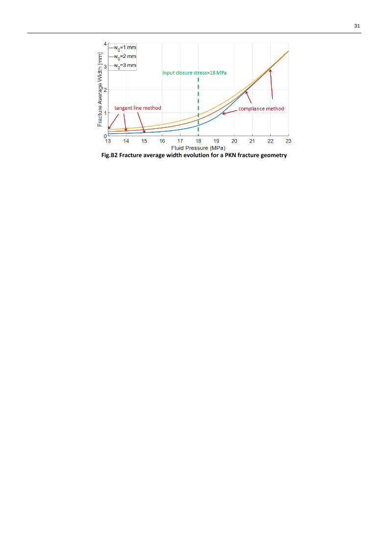
31

Fig.B2 Fracture average width evolution for a PKN fracture geometry