New trends in coupled simulations featuring domain decomposition and metacomputing

Mathematical Modelling and Numerical Analysis ESAIM: M2AN

Modelisation Mathematique et Analyse Numerique M2AN, Vol. 36, No 5, 2002, pp. 953–970

DOI: 10.1051/m2an:2002043

NEW TRENDS IN COUPLED SIMULATIONS FEATURING DOMAINDECOMPOSITION AND METACOMPUTING

Philippe d’Anfray1, Laurence Halpern

2and Juliette Ryan

3

Abstract. In this paper we test the feasibility of coupling two heterogeneous mathematical modelingintegrated within two different codes residing on distant sites. A prototype is developed using Schwarztype domain decomposition as the mathematical tool for coupling. The computing technology for cou-pling uses a CORBA environment to implement a distributed client-server programming model. Domaindecomposition methods are well suited to reducing complex physical phenomena into a sequence ofparallel subproblems in time and space. The whole process is easily tuned to underlying hardwarerequirements.

Mathematics Subject Classification. 65M55, 65Y05.

Received: December 7, 2001. Revised: May 23, 2002.

1. Introduction

Within the realm of partial differential equations, multifields models can quite significantly reduce the problemcomplexity while increasing the numerical accuracy. The complexity may be due to heterogeneous physics,mathematics, discretisations, or heterogeneous computing environments.

A solution to the physical and mathematical aspect is domain decomposition methods, well suited to reducingcomplex physical phenomena into a sequence of subproblems in time and space easier to model and which tosome extent can be solved simultaneously.

Many tools have been developed recently to achieve such cooperative computing that often require thoroughmodifications of codes to integrate new functionalities for coupling and much thinking as to where and who isin charge of the coupling. The goal of the CORBA standards developed by the OMG (Object Management Group)is to simplify these procedures.

Recent extensions of Schwarz type domain decomposition to time decomposition allow greater flexibility interms of granularity of the computation. Time-space domains can be adjusted to the underlying computinghardware and networks.

The aim of this paper is to test the feasibility of this process, applied to heterogeneous mathematical modelingof the convection diffusion problem, running on different computing sites with the use of, and monitored by, theCORBA environment.

Keywords and phrases. Domain decomposition, evolution equations, coupling of applications, heterogeneous computations,distributed computing, meta-computing, CORBA.

1 CEA DTI-CISC, 91191 Gif-sur-Yvette Cedex France (on leave from ONERA DTIM-CHP) and LAGA, Universite Paris XIII,93430 Villetaneuse, France. e-mail: [email protected] LAGA, Universite Paris XIII, 93430 Villetaneuse, France. e-mail: [email protected] ONERA DTIM-CHP and LAGA, Universite Paris XIII, 93430 Villetaneuse, France. e-mail: [email protected]

c© EDP Sciences, SMAI 2002

954 PH. D’ANFRAY ET AL.

The first part of this paper describes the time and space domain decomposition technique involved, thesecond part is a description of the CORBA technology. Finally an application is presented with the case of aconvection diffusion problem around an airfoil. The domain is split into 2 subdomains, finite elements roundthe airfoil and finite differences in the far field, each domain being computed with two different codes coupledvia CORBA.

2. Tools in domain decomposition methods

Let (0, T ) be a bounded time interval, and Ω a domain in R2 with boundary Γ = ∂Ω. Let us consider the

convection diffusion equation

PU ≡ ∂U

∂t+ a · ∇U − ν∆U = 0 in Ω × (0, T ), (1)

associated with the initial data U(·, 0) = U0 in Ω at time 0 and the Dirichlet boundary condition U = 0on Γ = ∂Ω.

The viscosity ν is a strictly positive coefficient. The advection velocity a is a smooth function of x, in ourcase always non-zero in Ω.

A general technique to solve the latter is to first discretise in time with an implicit scheme such as the secondorder Crank-Nicolson scheme :

un+1 − un

∆t+

12

[a · ∇un+1 − ν∆un+1

]+

12

[a · ∇un − ν∆un] = 0 in Ω, (2)

where un is an approximation of U(·, tn). At each step n , un+1 is solution of a steady equation such as Lu = Fwhere

L ≡ 2∆t

+ a · ∇ − ν∆

and F =(

2∆t − a · ∇ + ν∆

)un.

In the rest of this paper, the quantity 2∆t will be denoted by c.

Fast solvers for steady problems can now be applied such as non-overlapping domain decomposition methodsusing Schwarz type algorithms designed in [4] which are presented in Section 2.1. Algorithms global in time,namely Schwarz waveform relaxation algorithms as designed in [2] will be presented in Section 2.2.

2.1. Steady problems

As stated previously, we are led to the problemLu ≡ (c + a · ∇ − ν∆)u = F in Ω

u = 0 on Γ = ∂Ω.(3)

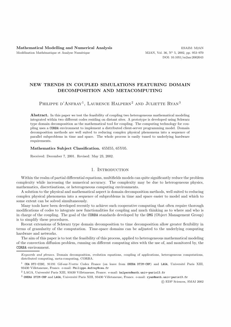
Let us split Ω in two subdomains: Ω = Ω1 ∪ Ω2 and denote Γ12 = Ω1 ∩ Ω2. On Γ12 , there are two unit normalsat each point: n1 is the outgoing normal to Ω1, n2 the outgoing normal to Ω2 and n1 +n2 = 0. Γ1 will denotethe part of Γ bounding Ω1 and Γ2 that of Γ bounding Ω2. We shall always suppose in the theoretical part, thatthe advection velocity a is constant and, to set matters, entering Ω2, i.e. that a · n1 > 0 along Γ12, althoughthe methodology carries over to more general situations (see [4]).

Let us now introduce the non-overlapping Schwarz algorithm.

Lvk+1 = F, in Ω1

vk+1 = 0 on Γ1

B1vk+1 = B1w

k on Γ12

Lwk+1 = F, in Ω2

wk+1 = 0 on Γ2

B2wk+1 = B2v

k on Γ12

(4)

NEW TRENDS IN COUPLED SIMULATIONS FEATURING DOMAIN DECOMPOSITION AND METACOMPUTING 955

Ω1

Ω2

n1

n2

Γ12

Γ1

Γ2

Figure 1. non-overlapping 2 domains decomposition.

where B1 et B2 are given byB1 =

∂

∂n1− a

ν+ p

B2 =∂

∂n2+ p

(5)

and p is a positive real number.Suppose Ω = R

2, Ω1 and Ω2 two half spaces delimited by Γ12 = (x, y), αx+βy = 0. For simplicity we shallwrite n = n1 = (α, β), so that n2 = −n. We shall perform the change of variables (X = αx+βy, Y = −βx+αy),and the two half spaces become Ω1 = (X, Y ), X < 0 and Ω2 = (X, Y ), X > 0. By a partial Fouriertransformation along the Y variable (the dual variable is denoted by ξ), we can calculate the iterate errorsV k = vk − u, W k = wk − u:

V k = αkeλ+x, W k = βkeλ−x

(λ+ − a

ν+ p

)αk+1 =

(λ− − a

ν+ p

)βk

(−λ− + p)βk+1 = (−λ+ + p)αk

where λ± are the roots of the characteristic polynomial

P (iξ; λ) = −νλ2 + a · nλ +(c + ia · τ ξ + νξ2

)

such that λ+(iξ) > 0 and λ−(iξ) < 0, where τ denotes the unit vector tangent to the interface such that(n, τ ) = +π/2.

The convergence rate is thus given by:

δ(iξ) =λ+(iξ) − p

λ−(iξ) − p· (6)

In [3], optimization of the convergence rate was proved to be successful, for more general transmission conditions.We choose an optimal value of p defined by

infp∈R+

supξ∈[ξ0,ξ1]

|δ(iξ)| (7)


where ξ0 is related to the length of the Y interval, ξ0 = πL , and ξ1 to the Y discretisation, ξ1 = π

∆Y . There is aunique popt minimizing the convergence rate, and it is characterized by δ(iξ0) = δ(iξ1) [5].

2.2. Evolution equations

An opposite approach has been proposed in [1]: the evolution equation itself is solved with a domain decom-position technique allowing for different time steps in each subdomain.

Let us resume the evolution equation

PU ≡ ∂U

∂t+ a · ∇U − ν∆U = 0 in Ω × (0, T ),

associated with the initial data U(·, 0) = U0 in Ω at time 0 and the Dirichlet boundary condition U = 0on Γ = ∂Ω. A global Schwarz algorithm in time can be developed in the two subdomains Ω1 × (0, T ), andΩ2 × (0, T ),

Pvk+1 = 0, in Ω1 × (0, T )vk+1(., 0) = U0 in Ω1

vk+1 = 0 on Γ1 × (0, T )B1v

k+1 = B1wk on Γ12 × (0, T )

(8)

Pwk+1 = 0, in Ω2 × (0, T )wk+1(., 0) = U0 in Ω1

wk+1 = 0 on Γ2 × (0, T )B2w

k+1 = B2vk on Γ12 × (0, T )

(9)

with the transmission operators given in (5). Again, in the case of two nonoverlapping half spaces, the error canbe identified through a Fourier transform (parameter ξ) in the tangential direction and a Laplace transform intime (parameter s with η = (s) ≥ η0 > 0).

More precisely, the partial Fourier transform in relation to Y and the Laplace transform in relation to t isdefined as:

u(x, ξ, s) =12π

∫R

∫R+

u(x, Y, t)e−iξY −stdY dt, s = η + iω, η ≥ η0.

The new convergence rate is δ(iξ, s) given formally by (6), where λ±(iξ, s) are now the roots of the characteristicpolynomial

P (iξ, s; λ) = −νλ2 + a · nλ +(c + ia · τξ + νξ2

).

The optimal value of p is now chosen so as to minimize

supξ∈[ξ0,ξ1],η≥η0,ω∈[ω0,ω1]

|δ(iξ, s)|

where ξ0 is related to the length of the Y interval, ξ0 = πL , and ξ1 to the Y discretisation, ξ1 = π

∆Y .In the same way, ω0 = π

T and ω1 = π∆T while η0 is chosen arbitrarily small.

For analyticity reasons, it is sufficient to make sure of an upper bound for η = η0 and p is computed to realize

infp∈R+

supξ∈[ξ0,ξ1],η=η0,ω∈[ω0,ω1]

|δ(iξ, s)|. (10)

This ends the presentation of the mathematical coupling. We now proceed to introduce the coupling technology.


3. Metacomputing

Development of software and hardware technologies has lead to the new paradigm of distributed or metacomputing. Object Oriented programming, client server model and software bus paradigm will be used toset up a new class of applications which might involve several simulation codes running on different sites andmultiple interacting users. One key point here is to be able to deal with heterogeneity of computing languages,operating systems and hardware platforms.

In this framework applications are seen as “object-servers” that interact transparently through the network.We introduce briefly some useful programming and run time models for distributed applications.

3.1. Programming and run time models

The first step is to encapsulate our applications in “objects”. An object has attributes –mainly the encap-sulated data– which define its state and a behavior described by its methods –or procedures–. In a generalobject oriented programming model one sends “messages” to objects to request execution of a local method.Hence, as described in the last sentence, typical objects are “servers”. They are able to perform a given task,i.e. “provide a service” upon reception of a message, i.e. “upon request from a client”.

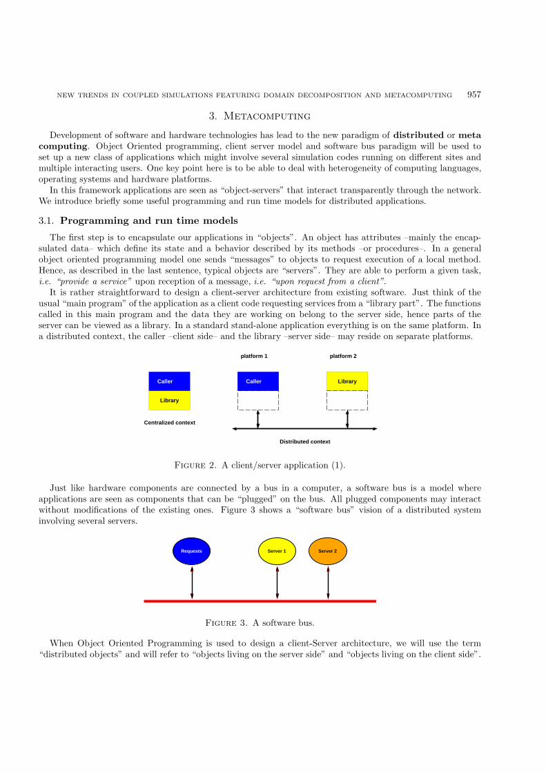
It is rather straightforward to design a client-server architecture from existing software. Just think of theusual “main program” of the application as a client code requesting services from a “library part”. The functionscalled in this main program and the data they are working on belong to the server side, hence parts of theserver can be viewed as a library. In a standard stand-alone application everything is on the same platform. Ina distributed context, the caller –client side– and the library –server side– may reside on separate platforms.

Caller

Library

platform 1 platform 2

Caller Library

Distributed context

Centralized context

Figure 2. A client/server application (1).

Just like hardware components are connected by a bus in a computer, a software bus is a model whereapplications are seen as components that can be “plugged” on the bus. All plugged components may interactwithout modifications of the existing ones. Figure 3 shows a “software bus” vision of a distributed systeminvolving several servers.

Requests Server 1 Server 2

Figure 3. A software bus.

When Object Oriented Programming is used to design a client-Server architecture, we will use the term“distributed objects” and will refer to “objects living on the server side” and “objects living on the client side”.


Client

(operations)

possible results Object Server

Objectinterface("Proxy")

Requests

Invocation

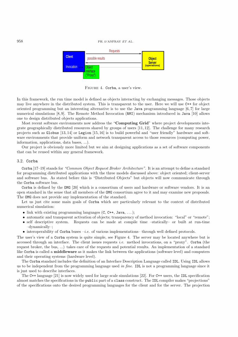
Figure 4. Corba, a user’s view.

In this framework, the run time model is defined as objects interacting by exchanging messages. Those objectsmay live anywhere in the distributed system. This is transparent to the user. Here we will use C++ for objectoriented programming but an interesting alternative is to use the Java programming language [6, 7] for largenumerical simulations [8, 9]. The Remote Method Invocation (RMI) mechanism introduced in Java [10] allowsone to design distributed objects applications.

Most recent software environments now address the “Computing Grid” where project developments inte-grate geographically distributed resources shared by groups of users [11, 12]. The challenge for many researchprojects such as Globus [13, 14] or Legion [15, 16] is to build powerful and “user friendly” hardware and soft-ware environments that provide uniform and network transparent access to those resources (computing power,information, applications, data bases, ...).

Our project is obviously more limited but we aim at designing applications as a set of software componentsthat can be reused within any general framework.

3.2. Corba

Corba [17–19] stands for “Common Object Request Broker Architecture”. It is an attempt to define a standardfor programming distributed applications with the three models discussed above: object oriented; client-serverand software bus. As stated before this is “Distributed Objects” but objects will now communicate throughthe Corba software bus.

Corba is defined by the OMG [20] which is a consortium of users and hardware or software vendors. It is anopen standard in the sense that all members of the OMG consortium agree to it and may examine new proposals.The OMG does not provide any implementation of the standard.

Let us just cite some main goals of Corba which are particularly relevant to the context of distributednumerical simulation:

• link with existing programming languages (C, C++, Java, . . . );• automatic and transparent activation of objects; transparency of method invocation: “local” or “remote”;• self descriptive system. Requests can be made at compile time –statically– or built at run-time

–dynamically–;• interoperability of Corba buses –i.e. of various implementations– through well defined protocols.

The user’s view of a Corba system is quite simple, see Figure 4. The server may be located anywhere but isaccessed through an interface. The client issues requests i.e. method invocations, on a “proxy”. Corba (therequest broker, the bus, ...) takes care of the requests and potential results. An implementation of a standardlike Corba is called a middleware as it makes the link between the applications (software level) and computersand their operating systems (hardware level).

The Corba standard includes the definition of an Interface Description Language called IDL. Using IDL allowsus to be independent from the programming language used in fine. IDL is not a programming language since itis just used to describe interfaces.

The C++ language [21] is now widely used for large scale simulations [22]. For C++ users, the IDL specificationalmost matches the specifications in the public part of a class construct. The IDL compiler makes “projections”of the specifications onto the desired programming languages for the client and for the server. The projection


IDLspecification

"Client side projection" "Server side projection"

Client interface"Stub"

user written codegenerated code

Server implementationClient code

Server interface"Skeleton"

"use" "realize"

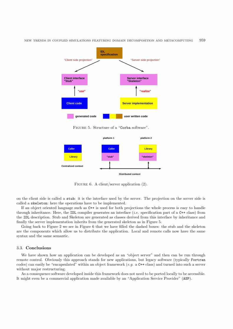
Figure 5. Structure of a “Corba software”.

"stub" "skeleton"

Caller

Library

platform 1 platform 2

Caller Library

Distributed context

Centralized context

Figure 6. A client/server application (2).

on the client side is called a stub: it is the interface used by the server. The projection on the server side iscalled a skeleton: here the operations have to be implemented.

If an object oriented language such as C++ is used for both projections the whole process is easy to handlethrough inheritance. Here, the IDL compiler generates an interface (i.e. specification part of a C++ class) fromthe IDL description. Stub and Skeleton are generated as classes derived from this interface by inheritance andfinally the server implementation inherits from the generated skeleton as in Figure 5.

Going back to Figure 2 we see in Figure 6 that we have filled the dashed boxes: the stub and the skeletonare the components which allow us to distribute the application. Local and remote calls now have the samesyntax and the same semantic.

3.3. Conclusions

We have shown how an application can be developed as an “object server” and then can be run throughremote control. Obviously this approach stands for new applications, but legacy software (typically Fortrancodes) can easily be “encapsulated” within an object framework (e.g. a C++ class) and turned into such a serverwithout major restructuring.

As a consequence software developed inside this framework does not need to be ported locally to be accessible.It might even be a commercial application made available by an “Application Service Provider” (ASP).


Once a server is developed, it is ready to be used as a component within a distributed application. Of coursesnew services will be needed for the components to communicate. It remains now to test the feasibility of thistechnology on a domain decomposition test case.

4. Application

An important aspect of domain decomposition is that it allows for geometric simplification with differentdiscretisations along with various modelisations. Complex geometrical elements are time consuming and shouldbe as few as possible. A typical problem is meshing with smoothness the connection of a wing to the fuselage,or any complex body within a large regular domain. Our test case concerns the coupling of finite elements withfinite differences discretisations of a same equation, relevant to this problem.

4.1. The test case

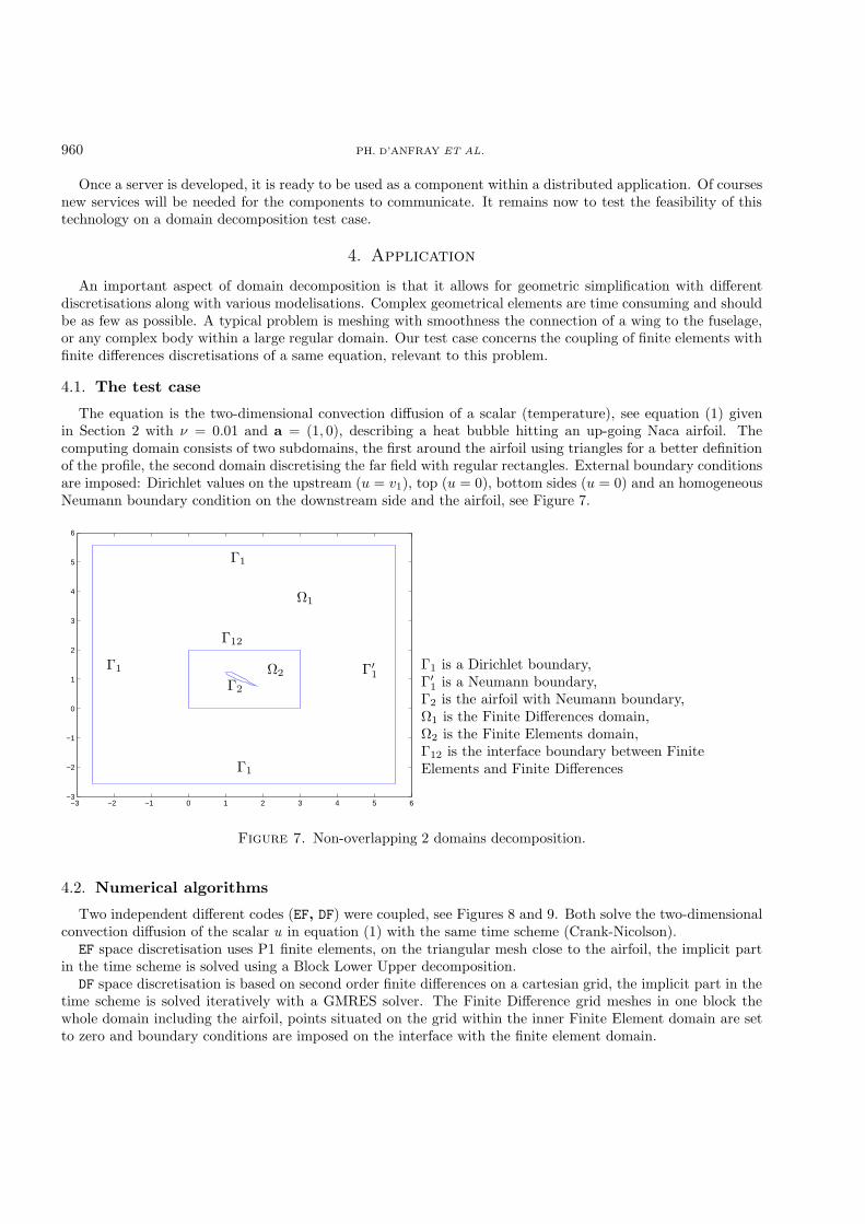
The equation is the two-dimensional convection diffusion of a scalar (temperature), see equation (1) givenin Section 2 with ν = 0.01 and a = (1, 0), describing a heat bubble hitting an up-going Naca airfoil. Thecomputing domain consists of two subdomains, the first around the airfoil using triangles for a better definitionof the profile, the second domain discretising the far field with regular rectangles. External boundary conditionsare imposed: Dirichlet values on the upstream (u = v1), top (u = 0), bottom sides (u = 0) and an homogeneousNeumann boundary condition on the downstream side and the airfoil, see Figure 7.

−3 −2 −1 0 1 2 3 4 5 6−3

−2

−1

0

1

2

3

4

5

6

Γ12

Γ1

Γ1

Γ1

Γ′1

Γ2

Ω1

Ω2Γ1 is a Dirichlet boundary,Γ′

1 is a Neumann boundary,Γ2 is the airfoil with Neumann boundary,Ω1 is the Finite Differences domain,Ω2 is the Finite Elements domain,Γ12 is the interface boundary between FiniteElements and Finite Differences

Figure 7. Non-overlapping 2 domains decomposition.

4.2. Numerical algorithms

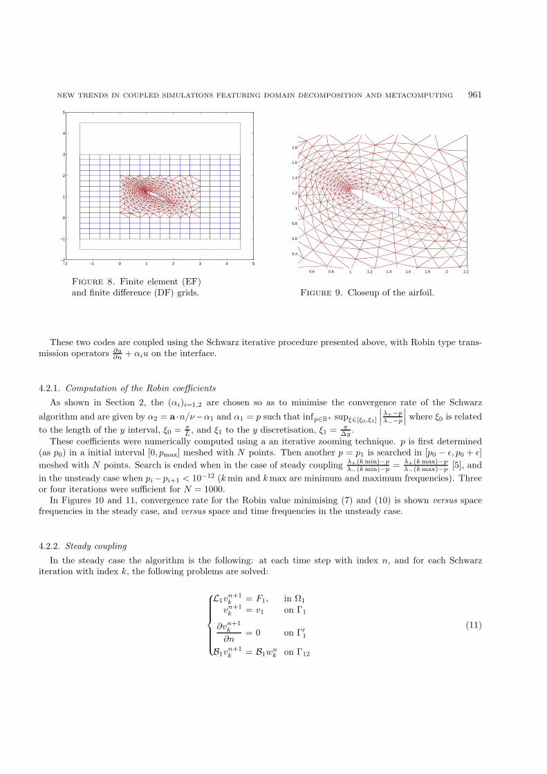
Two independent different codes (EF, DF) were coupled, see Figures 8 and 9. Both solve the two-dimensionalconvection diffusion of the scalar u in equation (1) with the same time scheme (Crank-Nicolson).

EF space discretisation uses P1 finite elements, on the triangular mesh close to the airfoil, the implicit partin the time scheme is solved using a Block Lower Upper decomposition.

DF space discretisation is based on second order finite differences on a cartesian grid, the implicit part in thetime scheme is solved iteratively with a GMRES solver. The Finite Difference grid meshes in one block thewhole domain including the airfoil, points situated on the grid within the inner Finite Element domain are setto zero and boundary conditions are imposed on the interface with the finite element domain.


−2 −1 0 1 2 3 4 5−2

−1

0

1

2

3

4

5

Figure 8. Finite element (EF)and finite difference (DF) grids.

0.6 0.8 1 1.2 1.4 1.6 1.8 2 2.2

0.4

0.6

0.8

1

1.2

1.4

1.6

1.8

Figure 9. Closeup of the airfoil.

These two codes are coupled using the Schwarz iterative procedure presented above, with Robin type trans-mission operators ∂u

∂n + αiu on the interface.

4.2.1. Computation of the Robin coefficients

As shown in Section 2, the (αi)i=1,2 are chosen so as to minimise the convergence rate of the Schwarz

algorithm and are given by α2 = a ·n/ν−α1 and α1 = p such that infp∈R+ supξ∈[ξ0,ξ1]

∣∣∣λ+−pλ−−p

∣∣∣ where ξ0 is relatedto the length of the y interval, ξ0 = π

L , and ξ1 to the y discretisation, ξ1 = π∆y .

These coefficients were numerically computed using a an iterative zooming technique. p is first determined(as p0) in a initial interval [0, pmax] meshed with N points. Then another p = p1 is searched in [p0 − ε, p0 + ε]meshed with N points. Search is ended when in the case of steady coupling λ+(k min)−p

λ−(k min)−p = λ+(k max)−pλ−(k max)−p [5], and

in the unsteady case when pi −pi+1 < 10−12 (k min and k max are minimum and maximum frequencies). Threeor four iterations were sufficient for N = 1000.

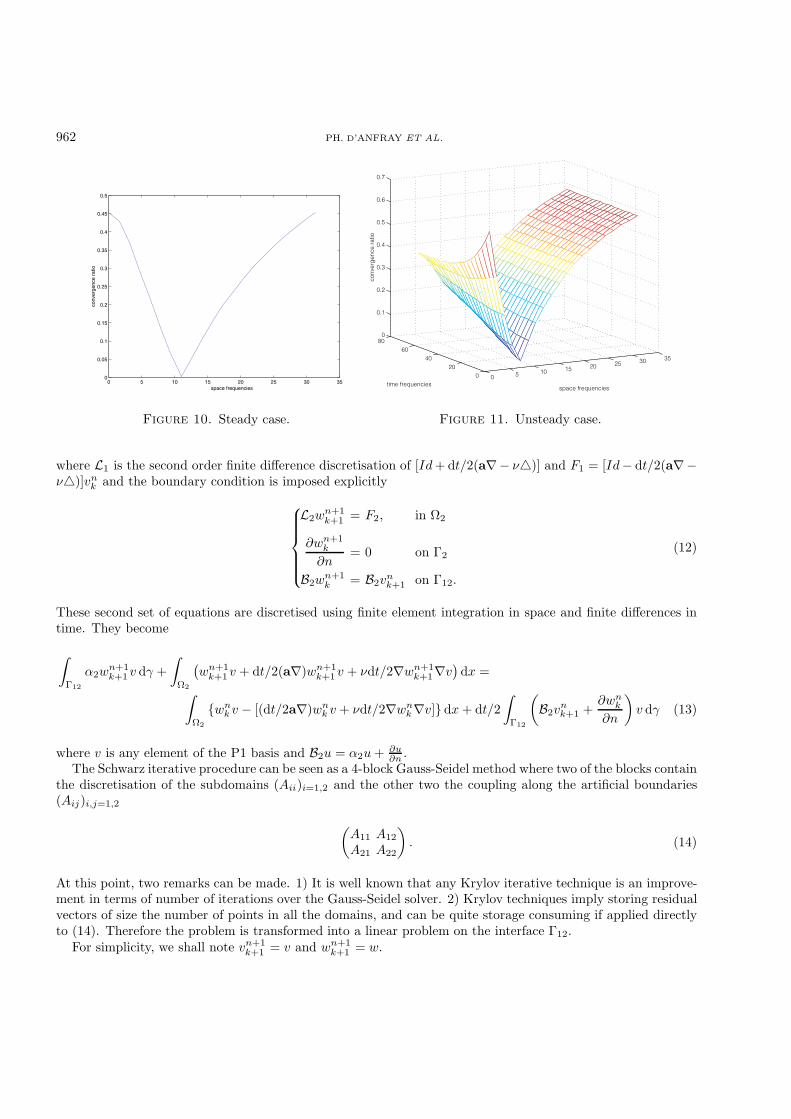
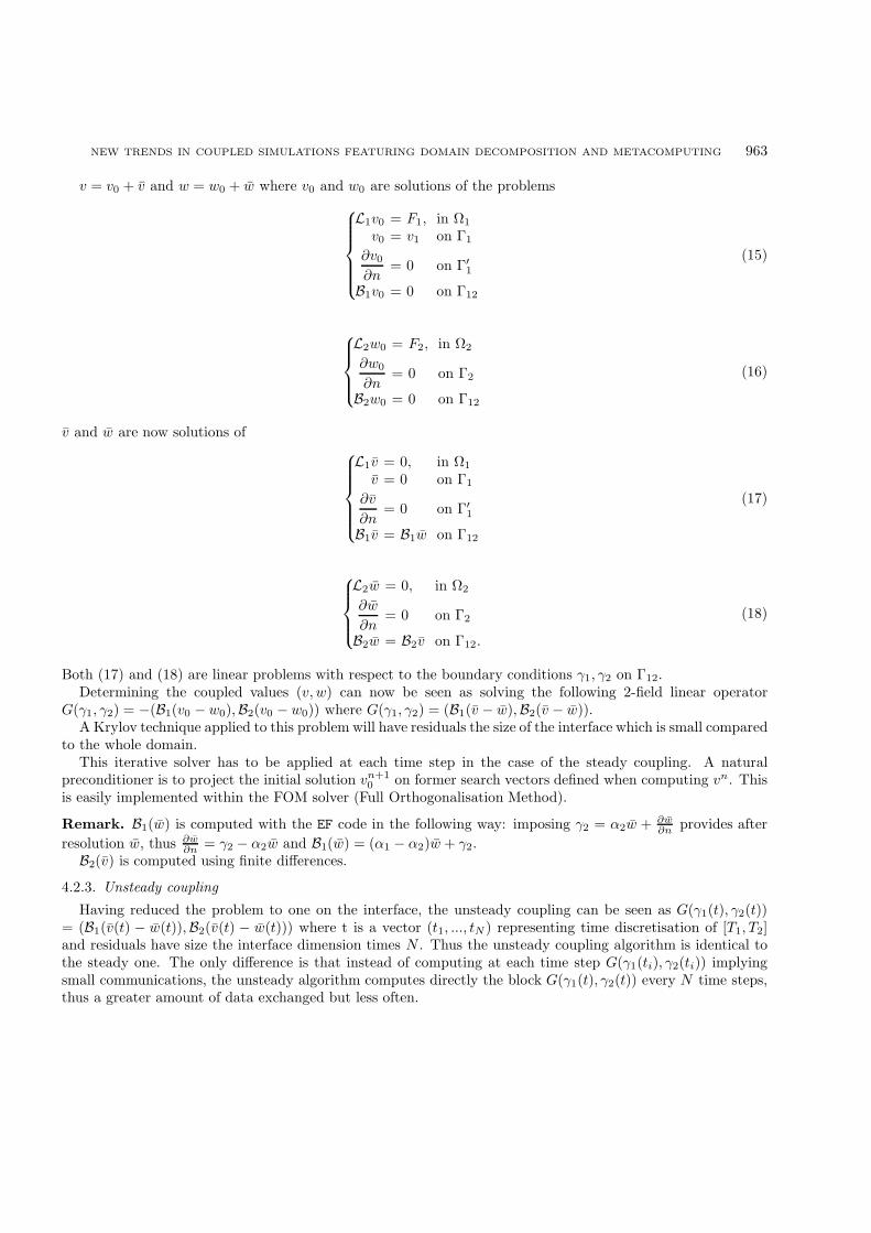
In Figures 10 and 11, convergence rate for the Robin value minimising (7) and (10) is shown versus spacefrequencies in the steady case, and versus space and time frequencies in the unsteady case.

4.2.2. Steady coupling

In the steady case the algorithm is the following: at each time step with index n, and for each Schwarziteration with index k, the following problems are solved:

L1vn+1k = F1, in Ω1

vn+1k = v1 on Γ1

∂vn+1k

∂n= 0 on Γ′

1

B1vn+1k = B1w

nk on Γ12

(11)


0 5 10 15 20 25 30 350

0.05

0.1

0.15

0.2

0.25

0.3

0.35

0.4

0.45

0.5

space frequencies

conv

erge

nce

ratio

Figure 10. Steady case. Figure 11. Unsteady case.

where L1 is the second order finite difference discretisation of [Id + dt/2(a∇− ν)] and F1 = [Id− dt/2(a∇−ν)]vn

k and the boundary condition is imposed explicitly

L2wn+1k+1 = F2, in Ω2

∂wn+1k

∂n= 0 on Γ2

B2wn+1k = B2v

nk+1 on Γ12.

(12)

These second set of equations are discretised using finite element integration in space and finite differences intime. They become

∫Γ12

α2wn+1k+1v dγ +

∫Ω2

(wn+1

k+1v + dt/2(a∇)wn+1k+1v + νdt/2∇wn+1

k+1∇v)dx =

∫Ω2

wnk v − [(dt/2a∇)wn

k v + νdt/2∇wnk∇v] dx + dt/2

∫Γ12

(B2v

nk+1 +

∂wnk

∂n

)v dγ (13)

where v is any element of the P1 basis and B2u = α2u + ∂u∂n .

The Schwarz iterative procedure can be seen as a 4-block Gauss-Seidel method where two of the blocks containthe discretisation of the subdomains (Aii)i=1,2 and the other two the coupling along the artificial boundaries(Aij)i,j=1,2

(A11 A12

A21 A22

). (14)

At this point, two remarks can be made. 1) It is well known that any Krylov iterative technique is an improve-ment in terms of number of iterations over the Gauss-Seidel solver. 2) Krylov techniques imply storing residualvectors of size the number of points in all the domains, and can be quite storage consuming if applied directlyto (14). Therefore the problem is transformed into a linear problem on the interface Γ12.

For simplicity, we shall note vn+1k+1 = v and wn+1

k+1 = w.


v = v0 + v and w = w0 + w where v0 and w0 are solutions of the problems

L1v0 = F1, in Ω1

v0 = v1 on Γ1

∂v0

∂n= 0 on Γ′

1

B1v0 = 0 on Γ12

(15)

L2w0 = F2, in Ω2

∂w0

∂n= 0 on Γ2

B2w0 = 0 on Γ12

(16)

v and w are now solutions of

L1v = 0, in Ω1

v = 0 on Γ1

∂v

∂n= 0 on Γ′

1

B1v = B1w on Γ12

(17)

L2w = 0, in Ω2

∂w

∂n= 0 on Γ2

B2w = B2v on Γ12.

(18)

Both (17) and (18) are linear problems with respect to the boundary conditions γ1, γ2 on Γ12.Determining the coupled values (v, w) can now be seen as solving the following 2-field linear operator

G(γ1, γ2) = −(B1(v0 − w0),B2(v0 − w0)) where G(γ1, γ2) = (B1(v − w),B2(v − w)).A Krylov technique applied to this problem will have residuals the size of the interface which is small compared

to the whole domain.This iterative solver has to be applied at each time step in the case of the steady coupling. A natural

preconditioner is to project the initial solution vn+10 on former search vectors defined when computing vn. This

is easily implemented within the FOM solver (Full Orthogonalisation Method).

Remark. B1(w) is computed with the EF code in the following way: imposing γ2 = α2w + ∂w∂n provides after

resolution w, thus ∂w∂n = γ2 − α2w and B1(w) = (α1 − α2)w + γ2.

B2(v) is computed using finite differences.

4.2.3. Unsteady coupling

Having reduced the problem to one on the interface, the unsteady coupling can be seen as G(γ1(t), γ2(t))= (B1(v(t) − w(t)),B2(v(t) − w(t))) where t is a vector (t1, ..., tN ) representing time discretisation of [T1, T2]and residuals have size the interface dimension times N . Thus the unsteady coupling algorithm is identical tothe steady one. The only difference is that instead of computing at each time step G(γ1(ti), γ2(ti)) implyingsmall communications, the unsteady algorithm computes directly the block G(γ1(t), γ2(t)) every N time steps,thus a greater amount of data exchanged but less often.


0 5 10 1510

8

6

4

2

0Steady case, 10 time steps

Iterations

Log

Err

or

No preconditioner

With preconditioner

0 5 10 1510

8

6

4

2

0Steady case, 20 time steps

Iterations

Log

Err

or

No preconditioner

With preconditioner

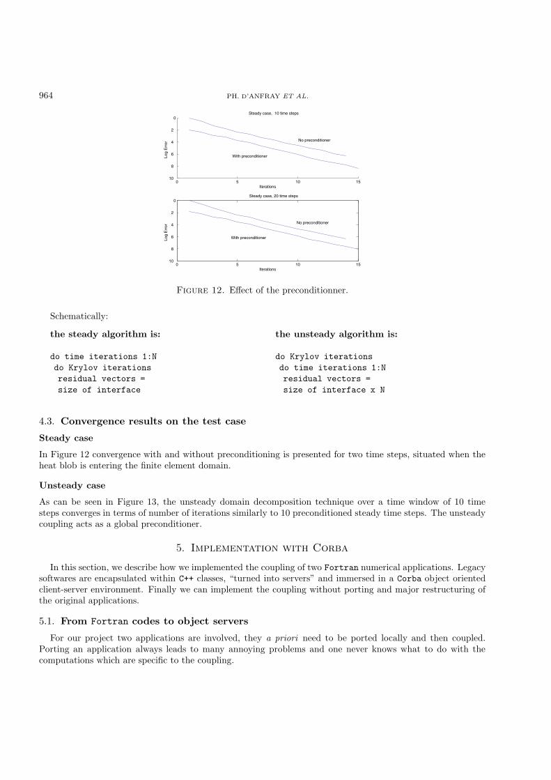
Figure 12. Effect of the preconditionner.

Schematically:

the steady algorithm is:

do time iterations 1:Ndo Krylov iterationsresidual vectors =size of interface

the unsteady algorithm is:

do Krylov iterationsdo time iterations 1:Nresidual vectors =size of interface x N

4.3. Convergence results on the test case

Steady case

In Figure 12 convergence with and without preconditioning is presented for two time steps, situated when theheat blob is entering the finite element domain.

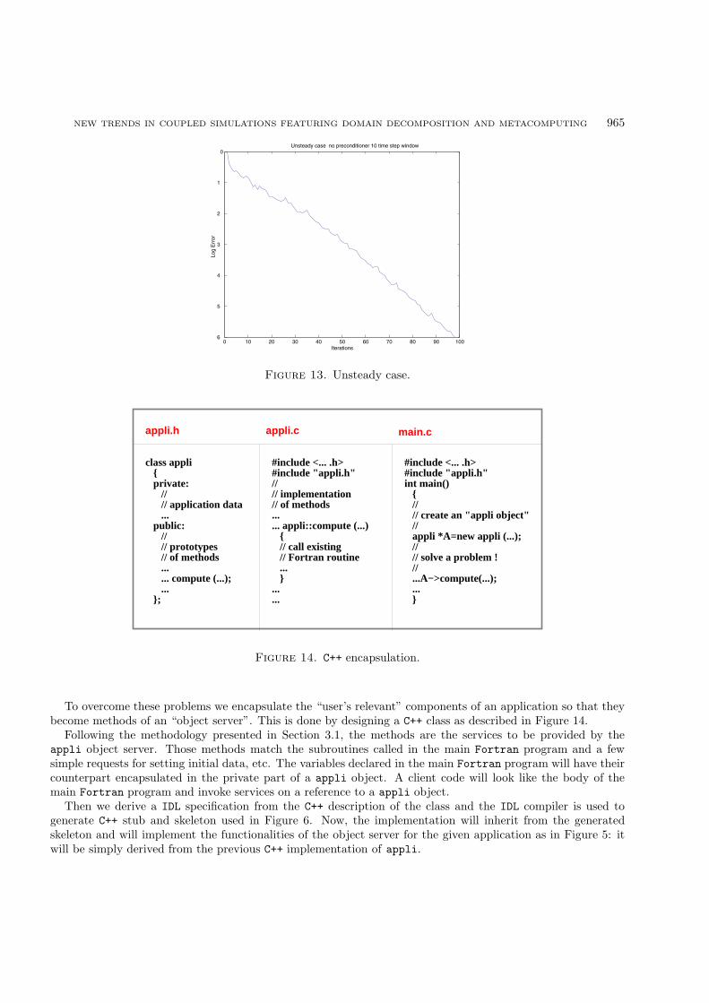
Unsteady case

As can be seen in Figure 13, the unsteady domain decomposition technique over a time window of 10 timesteps converges in terms of number of iterations similarly to 10 preconditioned steady time steps. The unsteadycoupling acts as a global preconditioner.

5. Implementation with Corba

In this section, we describe how we implemented the coupling of two Fortran numerical applications. Legacysoftwares are encapsulated within C++ classes, “turned into servers” and immersed in a Corba object orientedclient-server environment. Finally we can implement the coupling without porting and major restructuring ofthe original applications.

5.1. From Fortran codes to object servers

For our project two applications are involved, they a priori need to be ported locally and then coupled.Porting an application always leads to many annoying problems and one never knows what to do with thecomputations which are specific to the coupling.


0 10 20 30 40 50 60 70 80 90 1006

5

4

3

2

1

0Unsteady case no preconditioner 10 time step window

Iterations

Log

Err

or

Figure 13. Unsteady case.

appli.h

class appli private: // // application data ... public: // // prototypes // of methods ... ... compute (...); ... ;

appli.c main.c

#include <... .h>#include "appli.h"int main() // // create an "appli object" // appli *A=new appli (...); // // solve a problem ! // ...A−>compute(...); ...

#include <... .h>#include "appli.h"// // implementation// of methods...... appli::compute (...) // call existing // Fortran routine ... ......

Figure 14. C++ encapsulation.

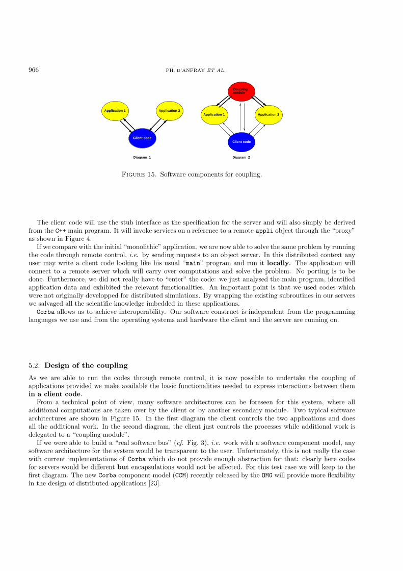
To overcome these problems we encapsulate the “user’s relevant” components of an application so that theybecome methods of an “object server”. This is done by designing a C++ class as described in Figure 14.

Following the methodology presented in Section 3.1, the methods are the services to be provided by theappli object server. Those methods match the subroutines called in the main Fortran program and a fewsimple requests for setting initial data, etc. The variables declared in the main Fortran program will have theircounterpart encapsulated in the private part of a appli object. A client code will look like the body of themain Fortran program and invoke services on a reference to a appli object.

Then we derive a IDL specification from the C++ description of the class and the IDL compiler is used togenerate C++ stub and skeleton used in Figure 6. Now, the implementation will inherit from the generatedskeleton and will implement the functionalities of the object server for the given application as in Figure 5: itwill be simply derived from the previous C++ implementation of appli.


Application 1 Application 2Application 1 Application 2

Client codeClient code

Coupling module

Diagram 2Diagram 1

Figure 15. Software components for coupling.

The client code will use the stub interface as the specification for the server and will also simply be derivedfrom the C++ main program. It will invoke services on a reference to a remote appli object through the “proxy”as shown in Figure 4.

If we compare with the initial “monolithic” application, we are now able to solve the same problem by runningthe code through remote control, i.e. by sending requests to an object server. In this distributed context anyuser may write a client code looking like his usual “main” program and run it locally. The application willconnect to a remote server which will carry over computations and solve the problem. No porting is to bedone. Furthermore, we did not really have to “enter” the code: we just analysed the main program, identifiedapplication data and exhibited the relevant functionalities. An important point is that we used codes whichwere not originally developped for distributed simulations. By wrapping the existing subroutines in our serverswe salvaged all the scientific knowledge imbedded in these applications.

Corba allows us to achieve interoperability. Our software construct is independent from the programminglanguages we use and from the operating systems and hardware the client and the server are running on.

5.2. Design of the coupling

As we are able to run the codes through remote control, it is now possible to undertake the coupling ofapplications provided we make available the basic functionalities needed to express interactions between themin a client code.

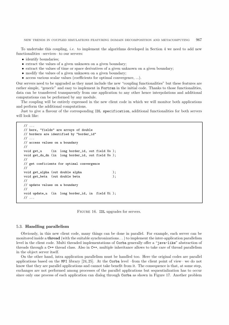
From a technical point of view, many software architectures can be foreseen for this system, where alladditional computations are taken over by the client or by another secondary module. Two typical softwarearchitectures are shown in Figure 15. In the first diagram the client controls the two applications and doesall the additional work. In the second diagram, the client just controls the processes while additional work isdelegated to a “coupling module”.

If we were able to build a “real software bus” (cf. Fig. 3), i.e. work with a software component model, anysoftware architecture for the system would be transparent to the user. Unfortunately, this is not really the casewith current implementations of Corba which do not provide enough abstraction for that: clearly here codesfor servers would be different but encapsulations would not be affected. For this test case we will keep to thefirst diagram. The new Corba component model (CCM) recently released by the OMG will provide more flexibilityin the design of distributed applications [23].


To undertake this coupling, i.e. to implement the algorithms developed in Section 4 we need to add newfunctionalities –services– to our servers:

• identify boundaries;• extract the values of a given unknown on a given boundary;• extract the values of time or space derivatives of a given unknown on a given boundary;• modify the values of a given unknown on a given boundary;• access various scalar values (coefficients for optimal convergence, ...).

Our servers need to be upgraded as they must include the new “coupling functionalities” but these features arerather simple, “generic” and easy to implement in Fortran in the initial code. Thanks to those functionalities,data can be transferred transparently from one application to any other hence interpolations and additionalcomputations can be performed by any module.

The coupling will be entirely expressed in the new client code in which we will monitor both applicationsand perform the additional computations.

Just to give a flavour of the corresponding IDL specification, additional functionalities for both serverswill look like:

// ...

// here, "fields" are arrays of double

// borders are identified by "border_id"

// ...

// access values on a boundary

//

void get_u (in long border_id, out field Uo );

void get_du_dn (in long border_id, out field Uo );

//

// get coeficients for optimal convergence

//

void get_alpha (out double alpha );

void get_beta (out double beta );

//

// update values on a boundary

//

void update_u (in long border_id, in field Ui );

// ...

Figure 16. IDL upgrades for servers.

5.3. Handling parallelism

Obviously, in this new client code, many things can be done in parallel. For example, each server can bemonitored inside a thread (with the suitable synchronizations. . . ) to implement the inter-application parallelismlevel in the client code. Multi threaded implementations of Corba generally offer a “java-like” abstraction ofthreads through a C++ thread class. Also in C++, multiple inheritance allows to take care of thread parallelismin the object server itself.

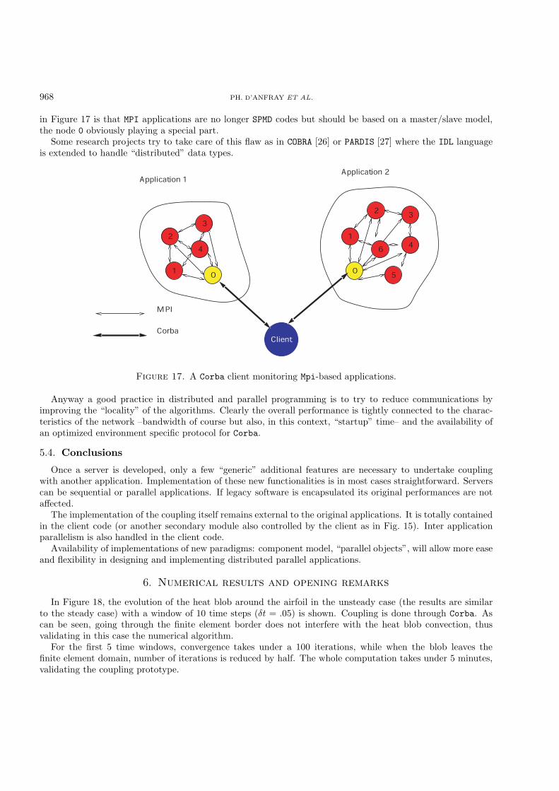
On the other hand, intra application parallelism must be handled too. Here the original codes are parallelapplications based on the MPI library [24, 25]. At the Corba level –from the client point of view– we do notknow that they are parallel applications and cannot take benefit from it. The consequence is that, at some step,exchanges are not performed among processes of the parallel applications but sequentialization has to occursince only one process of each application can dialog through Corba as shown in Figure 17. Another problem


in Figure 17 is that MPI applications are no longer SPMD codes but should be based on a master/slave model,the node 0 obviously playing a special part.

Some research projects try to take care of this flaw as in COBRA [26] or PARDIS [27] where the IDL languageis extended to handle “distributed” data types.

Figure 17. A Corba client monitoring Mpi-based applications.

Anyway a good practice in distributed and parallel programming is to try to reduce communications byimproving the “locality” of the algorithms. Clearly the overall performance is tightly connected to the charac-teristics of the network –bandwidth of course but also, in this context, “startup” time– and the availability ofan optimized environment specific protocol for Corba.

5.4. Conclusions

Once a server is developed, only a few “generic” additional features are necessary to undertake couplingwith another application. Implementation of these new functionalities is in most cases straightforward. Serverscan be sequential or parallel applications. If legacy software is encapsulated its original performances are notaffected.

The implementation of the coupling itself remains external to the original applications. It is totally containedin the client code (or another secondary module also controlled by the client as in Fig. 15). Inter applicationparallelism is also handled in the client code.

Availability of implementations of new paradigms: component model, “parallel objects”, will allow more easeand flexibility in designing and implementing distributed parallel applications.

6. Numerical results and opening remarks

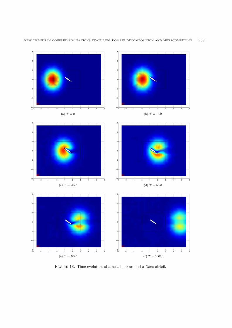
In Figure 18, the evolution of the heat blob around the airfoil in the unsteady case (the results are similarto the steady case) with a window of 10 time steps (δt = .05) is shown. Coupling is done through Corba. Ascan be seen, going through the finite element border does not interfere with the heat blob convection, thusvalidating in this case the numerical algorithm.

For the first 5 time windows, convergence takes under a 100 iterations, while when the blob leaves thefinite element domain, number of iterations is reduced by half. The whole computation takes under 5 minutes,validating the coupling prototype.


(a) T = 0 (b) T = 10δt

(c) T = 20δt (d) T = 50δt

(e) T = 70δt (f) T = 100δt

Figure 18. Time evolution of a heat blob around a Naca airfoil.


To conclude, several remarks can be made:First, one of the key points of the domain decomposition method presented here is its great pliability in

terms of border exchanges and local computation, thus allowing better adaptability to the hardware. By addingthe time dimension, communications can be adjusted to latency and bandwidth, independently of the spacesize of the domains. It is particularly well-suited to distributed computing. Connections with high latency andlarge bandwidth will be most effective with large time windows, and data transfers can be overlapped by localcomputations. Low latency and small bandwidth systems can work on a the steady coupling (a one time stepwindow) without modifying the precision of the results.

Secondly, this work has shown the feasibility of coupling heterogeneous methods on distant sites. Thesoftware technology used is simple and provides immediate access to the codes. In this context the coupling isnon-intrusive and is described in an external module.

Finally, such techniques allow fast prototyping of new algorithms and methods and is a step towards totalflexibility in CFD and other fields of numerical computations.

References

[1] M. Gander and L. Halpern, Methodes de relaxation d’ondes (SWR) pour l’equation de la chaleur en dimension 1 (submittedto CRAS).

[2] M.J. Gander, L. Halpern and F. Nataf, Optimal convergence for overlapping and non-overlapping Schwarz waveform relaxation,in Eleventh international Conference of Domain Decomposition Methods, C.-H. Lai, P. Bjørstad, M. Cross and O. WidlundEds. (1999).

[3] C. Japhet, Conditions aux limites artificielles et decomposition de domaine : methode OO2 (optimisee d’ordre 2). Applicationa la resolution de problemes en mecanique des fluides. These, Ecole Polytechnique (1997).

[4] C. Japhet, F. Nataf and F. Rogier, The Optimized Order 2 method. Application to convection-diffusion problems. FutureGeneration Computer Systems FUTURE 18 (2001).

[5] F. Nataf, communication personnelle.[6] M. Grand, Java Languare Reference. 2nd Edition, O’Reilly (1997), ISBN 1-56592-326-X.[7] The Java Programming Language, http://java.sun.com/.[8] Java Grande Forum, information at http://www.javagrande.org

[9] Java Numerics, information at http://math.nist.gov/javanumerics

[10] J. Farley, Java Distributed Computing. O’Reilly (1998), ISBN 1-565-92206-9.[11] GRID, The GRID Forum, http://www.gridforum.org/.[12] EGRID, The European Grid Forum, http://www.egrid.org[13] A. Chervenak, I. Foster, C. Kesselman, C. Salisbury and S. Tuecke, The Data Grid: Towards an Architecture for the Distributed

Management and Analysis of Large Scientific Datasets. Available on line at [14]. J. Network Comput. Appl. 23 (2001) 187–200.[14] The GlOBUS project, information at http://www.globus.org/.[15] S. Chapin, J. Karpovich and A. Grimshaw, The Legion Resource Management System, in Proc. of the 5th Workshop on Job

Scheduling Strategies for Parallel Processing (JSSPP’99). San Juan, Porto Rico (1999).[16] The LEGION project at the University of Virginia, USA, http://legion.virginia.edu/.[17] J. Siegel et al., CORBA Fundamentals and Programming. J. Wiley & Sons (1996), ISBN 0-471-12148-7.[18] M. Henning and S. Vinoski, Advanced CORBA Programming with C++. Addison-Wesley (1999), ISBN 0201379279.[19] Corba: Common Object Request Broker Architecture, information at http://www.corba.org

[20] OMG the Object Management Group, http://www.omg.org[21] B. Stroustrup, The C++ programming language. 3rd Edition, Addison-Wesley (1998), ISBN 0-201-88954-4.[22] J. Barton and L. Nackman, Scientific and Engineering C++. Addison-Wesley (1994).[23] OMG CCM Implementers Group, CORBA Component Model Tutorial, Document–ccm/02-04-01, available at http://www.omg.org

[24] W. Gropp, E. Lusk and A. Skjellum, Using MPI. 2nd Edition, MIT Press (1999), ISBN 0-262-57132-3.[25] MPI: Message Passing Interface, all documents can be retrived from http://www.mpi-forum.org/. For information and im-

plementations of the standard see http://www-unix.mcs.anl.gov/mpi/.[26] T. Priol, C. Rene and G. Alleon, Programming SCI Clusters Using Parallel CORBA Objects. INRIA-IRISA Report 3649

(1999).[27] K. Keahey and D. Gannon, PARDIS: CORBA-based Architecture for Application-level Parallel Distributed Computation, in

Proc. of Supercomputing’97 (1997).

New trends in coupled simulations featuring domain decomposition and metacomputing

Documents