HAL Id: tel-01315815 https://tel.archives-ouvertes.fr/tel-01315815 Submitted on 27 May 2016 HAL is a multi-disciplinary open access archive for the deposit and dissemination of sci- entific research documents, whether they are pub- lished or not. The documents may come from teaching and research institutions in France or abroad, or from public or private research centers. L’archive ouverte pluridisciplinaire HAL, est destinée au dépôt et à la diffusion de documents scientifiques de niveau recherche, publiés ou non, émanant des établissements d’enseignement et de recherche français ou étrangers, des laboratoires publics ou privés. New tone reservation PAPR reduction techniques for multicarrier systems Ralph Mounzer To cite this version: Ralph Mounzer. New tone reservation PAPR reduction techniques for multicarrier systems. Me- chanical engineering [physics.class-ph]. INSA de Rennes, 2015. English. NNT : 2015ISAR0029. tel-01315815

Welcome message from author
This document is posted to help you gain knowledge. Please leave a comment to let me know what you think about it! Share it to your friends and learn new things together.
Transcript

HAL Id: tel-01315815https://tel.archives-ouvertes.fr/tel-01315815
Submitted on 27 May 2016
HAL is a multi-disciplinary open accessarchive for the deposit and dissemination of sci-entific research documents, whether they are pub-lished or not. The documents may come fromteaching and research institutions in France orabroad, or from public or private research centers.
L’archive ouverte pluridisciplinaire HAL, estdestinée au dépôt et à la diffusion de documentsscientifiques de niveau recherche, publiés ou non,émanant des établissements d’enseignement et derecherche français ou étrangers, des laboratoirespublics ou privés.
New tone reservation PAPR reduction techniques formulticarrier systems
Ralph Mounzer
To cite this version:Ralph Mounzer. New tone reservation PAPR reduction techniques for multicarrier systems. Me-chanical engineering [physics.class-ph]. INSA de Rennes, 2015. English. �NNT : 2015ISAR0029�.�tel-01315815�

Thèse
THESE INSA Rennessous le sceau de l’Université européenne de Bretagne
pour obtenir le titre deDOCTEUR DE L’INSA DE RENNES
Spécialité : Electronique et Télécommunications
présentée par
Ralph MOUNZERECOLE DOCTORALE : MATISSELABORATOIRE : IETR
New Tone ReservationPAPR Reduction
Techniques forMulticarrier Systems
Thèse soutenue le 15.12.2015devant le jury composé de :
Jean-Michel NEBUSProfesseur à l’Université de Limoges / PrésidentGeneviève BAUDOIN,Professeur à l’ESIEE à Noisy Le Grand / RapporteurDaniel ROVIRASProfesseur au CNAM de Paris / RapporteurAlain UNTERSEEIngénieur chez Teamcast à Saint-Grégoire / ExaminateurYoussef NASSEREnseignant-Chercheur à l’Univ. Américaine de Beyrouth, Co-encadrantMatthieu CRUSSIEREMaître de Conférences à l’INSA de Rennes, Co-encadrantJean-François HELARDProfesseur à l’INSA de Rennes / Directeur de thèse


3 | P a g e
New Tone Reservation PAPR Reduction Techniques for Multicarrier Systems
Ralph MOUNZER
En partenariat avec


5 | P a g e
ACKNOWLEDGEMENT
I would like to express my gratitude to my supervisors Prof. Jean‐François
HELARD, Dr. Matthieu CRUSSIERE, and Dr. Youssef NASSER for their
continuous support and patience.
I would also like to thank the members of the jury Prof. Jean‐Michel NEBUS,
Prof. Geneviève BAUDOIN, Prof. Daniel ROVIRAS, and Mr. Alain UNTERSEE
for accepting to review my thesis and for their valuable feedback.
A special thanks to Rebecca who was always there during the most difficult
moments of my thesis.
I am deeply grateful to my parents for all of the sacrifices that they have
made on my behalf.


7 | P a g e
Table of Contents
RESUME EN FRANÇAIS I
GENERAL INTRODUCTION 25
OFDM AND DIGITAL VIDEO BROADCASTING 29
1.1 ORTHOGONAL FREQUENCY MULTIPLEXING SYSTEMS 29
1.1.1 HISTORY OF OFDM 29
1.1.2 INTER‐SYMBOL INTERFERENCE IN RF NETWORKS 31
1.1.3 MULTI CARRIER SYSTEMS 31
1.1.4 PRINCIPLE OF ORTHOGONAL FREQUENCY DIVISION MULTIPLEXING 32
1.1.5 OFDM WITH FREQUENCY SELECTIVE CHANNELS 33
1.1.6 INTER CHANNEL INTERFERENCE 34
1.1.7 GUARD INTERVAL 34
1.1.8 ENVELOPE FLUCTUATIONS IN MC SYSTEMS 34
1.1.9 ADVANTAGES AND LIMITATIONS 35
1.2 DIGITAL TERRESTRIAL TELEVISION BROADCASTING 35
1.2.1 ADVANCED TELEVISION SYSTEM COMMITTEE (ATSC) 36
1.2.2 DIGITAL TERRESTRIAL MULTIMEDIA BROADCASTING (DTMB) 36
1.2.3 INTEGRATED SERVICES DIGITAL BROADCASTING – TERRESTRIAL (ISDB‐T) 36
1.2.4 DIGITAL VIDEO BROADCASTING TERRESTRIAL 36
1.3 DVB‐T2 36
1.3.1 PHYSICAL LAYER PIPES 37
1.3.2 IFFT SIZE 38
1.3.3 FRAME STRUCTURE 38
1.3.4 FORWARD ERROR CORRECTION 39
1.3.5 ROTATED CONSTELLATIONS 40
1.3.6 SCATTERED AND CONTINUAL PILOTS 40
1.3.7 MULTIPLE INPUT SINGLE OUTPUT 41
1.3.8 MARKET DEPLOYMENT 42
1.4 CONCLUSION 42
HIGH POWER AMPLIFIERS AND PAPR REDUCTION TECHNIQUES 43
2.1 HIGH POWER AMPLIFIERS 43
2.1.1 POWER BALANCE AND GAIN 44
2.1.2 CLASSES 44
2.1.3 TRANSFER CHARACTERISTICS 44
2.1.4 EFFICIENCY 45
2.1.5 POWER AMPLIFIER MODELING 46
2.1.6 MODULATION ERROR RATE AND ERROR VECTOR MAGNITUDE 47
2.1.7 ADJACENT CHANNEL POWER RATIO 48
2.2 THE PAPR PROBLEM 49

8 | P a g e
2.2.1 INPUT BACK OFF 49
2.2.2 IBO AND MER 49
2.2.3 LINEARIZATION TECHNIQUES 49
2.2.4 LIMITING SIGNAL FLUCTUATIONS 50
2.2.5 PAPR DEFINITION 51
2.2.6 COMPLEMENTARY CUMULATIVE DISTRIBUTION FUNCTIONS OF THE PAPR OF OFDM SIGNALS 52
2.3 PAPR REDUCTION TECHNIQUES 52
2.3.1 AMPLITUDE CLIPPING AND FILTERING 52
2.3.2 CODING 52
2.3.3 GOLAY COMPLEMENTARY SEQUENCES 53
2.3.4 PARTIAL TRANSMIT SEQUENCE 54
2.3.5 SELECTED MAPPING TECHNIQUE 55
2.3.6 INTERLEAVING TECHNIQUE 55
2.3.7 TONE INJECTION 55
2.3.8 TONE RESERVATION 56
2.3.9 ACTIVE CONSTELLATION EXPANSION 60
2.3.10 COMPARISON OF VARIOUS PAPR TECHNIQUES 62
2.4 CONCLUSION 62
TONE RESERVATION: ANALYSIS AND WAYS FOR IMPROVEMENT 63
3.1 DVB‐T2 TR ANALYSIS 63
3.1.1 POWER CONTROL 63
3.1.2 FLOW CHARTS 66
3.1.3 ALGORITHM 67
3.1.4 IMPACT OF THE CLIPPING THRESHOLD 69
3.1.5 RESERVED TONES AND KERNEL GENERATION 70
3.1.6 IMPACT OF OVERSAMPLING 70
3.1.7 IMPACT OF THE IFFT SIZE ON THE NUMBER OF ITERATIONS 71
3.1.8 IMPACT OF THE POWER CONTROL ON THE NUMBER OF EXECUTED ITERATIONS 74
3.1.9 IMPACT OF HPA LINEARITY 76
3.1.10 SOCP 77
3.1.11 LIMITATIONS AND DRAWBACKS OF THE DVB‐T2 TR ALGORITHM 78
3.2 PARTIAL OVERSAMPLING AND FRACTIONAL SHIFTED KERNELS 78
3.2.1 PARTIAL OVERSAMPLING 79
3.2.2 FRACTIONAL SHIFTED PILOTS 79
3.2.3 POFSK PERFORMANCE 80
3.2.4 GENERALIZED PARTIAL OVERSAMPLED AND FRACTIONAL SHIFTED KERNELS 81
3.2.5 ALGORITHM 81
3.2.6 PERFORMANCE 83
3.3 DYNAMIC THRESHOLD AND ENHANCED PEAK SELECTION 85
3.3.1 DYNAMIC THRESHOLD 85
3.3.2 DYNAMIC THRESHOLD PERFORMANCE 86
3.3.3 ENHANCED PEAK SELECTION 87
3.3.4 ALGORITHM 88
3.3.5 EPS PERFORMANCE 89
3.3.6 PERFORMANCE OF EPS AND DT COMBINED 90
3.4 CONCLUSION 91

9 | P a g e
INDIVIDUAL CARRIER MULTIPLE PEAKS 93
4.1 INDIVIDUAL CARRIER MULTIPLE PEAKS 93
4.1.1 CONCEPT 93
4.1.2 NEW KERNEL DEFINITION 93
4.1.3 PERFORMANCE OF ICSP 94
4.1.4 PHASE OPTIMIZATION 95
4.1.5 COMPARISON WITH DVB‐T2 96
4.1.6 ALGORITHM 97
4.1.7 PERFORMANCE OF ICMP 98
4.2 GROUPED INDIVIDUAL CARRIER MULTIPLE PEAKS 100
4.2.1 ALGORITHM 102
4.2.2 COMPARISON WITH OKOP 103
4.2.3 GROUPED ICMP PERFORMANCE 103
4.3 PERFORMANCE AND COMPLEXITY USING A REAL PLATFORM 104
4.3.1 FIRST TEST BENCH ‐ MER 104
4.3.2 SECOND TEST BENCH ‐ POWER EFFICIENCY 108
4.3.3 COMPLEXITY 110
4.4 CONCLUSION 111
JOINT CHANNEL ESTIMATION AND PAPR REDUCTION SCHEME 113
5.1 INTRODUCTION 113
5.2 DEFINITIONS 114
5.3 CEPR TECHNIQUE 114
5.3.1 SEQUENCE DESIGN 114
5.3.2 PAPR REDUCTION 115
5.3.3 PILOTS RECOVERY 115
5.3.4 BLOCK DIAGRAM 117
5.3.5 ERROR DETECTION PROBABILITY OF CEPR 118
5.3.6 COMPLEXITY 118
5.4 FAST CEPR TECHNIQUE 119
5.4.1 SEQUENCE DESIGN 119
5.4.2 PAPR REDUCTION 120
5.4.3 COMPLEXITY 123
5.5 FAST SHIFTED CEPR TECHNIQUE 124
5.5.1 SEQUENCE DESIGN 124
5.5.2 PAPR REDUCTION 125
5.5.3 PILOT RECOVERY WITH FS‐CEPR 126
5.5.4 ERROR DETECTION PROBABILITY OF FS‐CEPR 127
5.5.5 COMPLEXITY 128
5.6 FAST INTERLEAVED CEPR TECHNIQUE 128
5.6.1 SEQUENCES DESIGN 129
5.6.2 PAPR REDUCTION 130
5.6.3 PILOT RECOVERY AND CHANNEL ESTIMATION 130
5.6.4 ERROR DETECTION PROBABILITY OF FI‐CEPR 131
5.6.5 COMPLEXITY 131
5.7 SIMULATIONS AND DISCUSSIONS 131

10 | P a g e
5.7.1 PAPR EFFECTIVE GAIN 132
5.7.2 F‐CEPR PERFORMANCE 132
5.7.3 IMPACT OF THE DISCRETE STEPS ON EDP PERFORMANCE 133
5.7.4 IMPACT OF M AND ON EDP PERFORMANCE 134
5.7.5 FS‐CEPR PERFORMANCE 135
5.7.6 FI‐CEPR PERFORMANCE 135
5.7.7 EDP PERFORMANCE 136
5.7.8 COMPARISON 137
5.8 CONCLUSION 137
CONCLUSION AND PROSPECTS 139
LIST OF FIGURES 143
LIST OF TABLES 147
BIBLIOGRAPHY 149
ANNEX A – RESERVED PILOTS POSITIONS 161
ANNEX B – TIME DOMAIN DERIVATION FOR F‐CEPR SEQUENCES 163

I | P a g e
Résumé en français
Depuis l’invention de la télévision au début du 20ème siècle son marché a connu une expansion constante. Les
revenus de l’industrie de la télévision ont dépassé les 407 milliards d’euros en 2014 et les projections pour 2018
sont estimées à 474.6 milliards d’euros. Aujourd’hui parmi les 1 554 millions de ménages qui consomment des
services de télévision, 1 055 millions sont équipés de récepteurs numériques, ce nombre incluant la réception
dite terrestre (TNT), la télévision par câble, la télévision par satellite et la télévision par accès internet (IPTV). La
pénétration de la télévision numérique a augmenté de 40.5% en 2010 à 67.2% en 2014.
Cette thèse porte sur l’optimisation de l’efficacité énergétique des systèmes de diffusion numérique en général
et de la télévision numérique en particulier. Pour cela, on étudie dans cette thèse la deuxième version du
standard européen « Digital Video Broadcasting for Terrestrial » (DVB‐T2). DVB‐T2 et son prédécesseur DVB‐T
sont largement déployés dans plus de 150 pays en Europe, Asie et Afrique.
DVB‐T2, comme plusieurs systèmes modernes de télécommunication (par exemple les systèmes ADSL, Wi‐MAX,
WiFi, DVB), a adopté la technique de transmission à porteuses multiples OFDM (Orthogonal Frequency Division
Multiplexing) en raison de sa robustesse naturelle face aux effets des canaux à trajets multiples, lui permettant
ainsi d'atteindre des niveaux élevés d'efficacité spectrale. Cependant, les signaux OFDM sont caractérisés par
un niveau important de fluctuation de leur enveloppe temporelle et sont par conséquent particulièrement
sensibles aux composantes non‐linéaires de la chaine de transmission. Notamment, sous l'effet de ces non‐
linéarités, les signaux OFDM sont sujets à de fortes distorsions dans la bande de transmission et hors bande de
transmission qui induisent respectivement une augmentation du taux d’erreur par bit (Bit Error Rate BER) et un
niveau supérieur d’interférence co‐canal.
L’amplificateur de puissance (High Power Amplifier HPA) constitue la source principale de non‐linéarité dans un
système typique de transmission. Selon le projet Energy Aware Radio and NeTwork Technologies (EARTH), le
HPA consomme 55% à 60% de la puissance totale d’une station de base d'une macrocellule d'un réseau 4G LTE
(Long Term Evolution). Ce pourcentage est encore plus élevé pour les systèmes de diffusion de télévision pour
lesquels la puissance de transmission peut atteindre 100 dBm (à comparer avec 40 dBm pour une station d'une
macrocellule LTE). Afin de limiter les distorsions des signaux OFDM, les concepteurs des systèmes radio sont
amenés à exploiter le HPA bien en deçà de sa zone optimale de rendement de puissance. On comprend alors
que l’efficacité énergétique des systèmes OFDM peut être améliorée en réduisant les fluctuations d'amplitude
des signaux à l’entrée du HPA.

II | P a g e
La métrique Peak to Average Power Ratio (PAPR) est largement utilisée pour quantifier le niveau de fluctuation
de puissance des signaux. Plusieurs techniques de réduction du PAPR ont été proposées dans la littérature. En
particulier, le standard DVB‐T2 a adopté deux techniques : la technique Tone Reservation (TR) et la technique
Active Constellation Extension (ACE). Ces deux techniques souffrent de plusieurs désavantages qui les rendent
trop complexes à implémenter sur une plateforme matérielle.
Une grande partie de cette thèse est liée au projet régional français Peak to Average Power Ratio Iterative
Compression Algorithm (PAPRICA) financé par la région Bretagne. Le but de PAPRICA est d’améliorer l’efficacité
énergétique des modulateurs DVB‐T2 en proposant des techniques nouvelles de réduction du PAPR de
complexité raisonnable pouvant être implémentées au sein de modulateurs DVB‐T2 du marché. Trois
partenaires participent au projet : TeamCast Technologies (un fabricant de modulateurs DVB), Kenta Electronic
(un fabricant d’amplificateurs de puissance) et INSA‐IETR (un laboratoire de recherche).
Chapitre 1 : OFDM et télévision numérique
Principe OFDM et fluctuations de puissance dans les systèmes multi‐porteuses
Les signaux multi‐porteuses, et les signaux OFDM en particulier, sont formés par des additions simultanées et
pondérées de plusieurs sous‐porteuses. Un signal OFDM peut être vu comme une somme de plusieurs variables
aléatoires indépendantes et identiquement distribuées (i.i.d.). Le théorème central limite établit que la loi de la
somme d’une suite de variables aléatoires i.i.d. converge vers la loi normale. Ceci implique, que pour un nombre
élevé de sous‐porteuses, la distribution de la partie réelle (et celle de la partie imaginaire) d’un signal OFDM
peut être considérée comme suivant une loi Gaussienne. On comprend alors que la différence d’amplitude entre
la valeur moyenne et la valeur maximale est plus importante pour les signaux multi‐porteuses que pour les
signaux mono‐porteuses. C’est pour cela que les systèmes multi‐porteuses sont caractérisés par des fluctuations
élevées de puissance. La Figure 1 montre les fluctuations d’amplitude de plusieurs signaux mono‐porteuses et
de leur somme.
Figure 1 – Fluctuations de puissance.
DVB‐T2
Le standard Digital Video Broadcasting (DVB‐T) a été créé dans les années 90 par un consortium européen. Les
études pour moderniser DVB‐T et offrir les services de télévision haute définition (High Definition Television
HDTV) pour les consommateurs européens de la manière la plus efficace ont commencé en 2006. Le Technical
Module on Next Generation DVB‐T (TM‐T2) a publié en Mars 2007 le cahier des charges pour DVB‐T2. Le but
était de créer un nouveau standard qui :

III | P a g e
prend avantage et réutilise l’infrastructure existante,
fournit au moins 30% de débit supplémentaire comparé avec un système DVB‐T,
permet un meilleur déploiement des réseaux mono‐fréquences (Single Frequency Network ‐ SFN)
fournit une robustesse ajustable par service,
est flexible dans l’allocation de la bande passante,
réduit le coût de transmission en fournissant des mécanismes de réduction du PAPR.
Pour répondre à ces exigences, plusieurs innovations ont été incluses dans le standard DVB‐T2. La Table 1
résume les différences majeures entre les systèmes DVB‐T et DVB‐T2.
Table 1 – Comparaison entre DVB‐T et DVB‐T2.
DVB‐T DVB‐T2
FEC Convolutional Coding +
Reed Solomon 1/2, 2/3, 3/4, 5/6, 7/8
LDPC +
BCH 1/2, 3/5, 2/3, 3/4, 4/5, 5/6
Modes QPSK, 16QAM, 64QAM QPSK, 16QAM, 64QAM, 256QAM
Intervalle de garde 1/4, 1/8, 1/16, 1/32 1/4, 19/128, 1/8, 19/256, 1/16, 1/32, 1/128
Taille de FFT 2K, 8K 1K, 2K, 4K, 8K, 16K, 32K
Schémas de pilotes 1 Pilot Pattern 8 Pilot Patterns: PP1 to PP8
% des pilotes
entrelacés 8% of total 1%, 2%, 4%, 8% of total
% des pilotes
continus 2.0% of total 0.4%‐2.4% (0.4%‐0.8% in 8K‐32K)
Largeur de bande 6, 7, 8 MHz 1.7, 5, 6, 7, 8, 10 MHz
Débit typique de
transmission 24 Mbit/s 40 Mbit/s
Débit maximum 31.7 Mbit/s
(using 8 MHz @20 dB C/N)
45.5 Mbit/s
(using 8 MHz @20 dB C/N)
Rapport C/N
nécessaire 16.7 dB @24 Mbit/s 10.8 dB @24 Mbit/s
La Figure 2 montre le déploiement des différents standards de télévision numérique dans le monde. DVB‐T2 a
été déployé au Royaume‐Uni en 2010. Aujourd'hui, presque tous les pays européens étudient ou exécutent un
plan de transfert du standard DVB‐T vers le standard DVB‐T2. Au total plus de 40 pays ont adopté le standard
DVB‐T2 et 28 l’on déjà déployé.
Figure 2 – Cartographie de déploiement des standards de télévision numérique terrestre dans le monde

IV | P a g e
Chapitre 2 : Amplificateur de puissance et réduction du PAPR
Dans ce chapitre on présente les caractéristiques des HPAs et on explique comment les fluctuations de puissance
des signaux OFDM peuvent impacter l’efficacité énergétique des HPAs. On introduit ensuite les différentes
techniques de réduction du PAPR proposées dans la littérature notamment la techniques TR adoptée par le
standard DVB‐T2.
Amplificateur de puissance
Un HPA prend en entrée un signal de puissance et génère un signal amplifié en sortie de puissance .
Pour fonctionner, l’amplificateur consomme une quantité d’énergie . Le processus d’amplification n’étant
pas idéal, c'est‐à‐dire de rendement inférieur à 1, une puissance est dissipée. Le bilan énergétique d’un HPA est alors donné par l’équation suivante :
Le gain du HPA est défini par :
L’efficacité énergétique est donnée par :
Soient le signal à l’entrée de l’amplificateur et le signal à sa sortie. Un HPA peut être modélisé par un
système sans mémoire comme suit :
. . .
où la fonction . représente la caractéristique amplitude à amplitude (AM/AM) du HPA, et la fonction . , .
représente la caractéristique amplitude à phase (AM/PM) du HPA.
Pour les amplificateurs de type Solid State Power Amplifier (SSPA), étudiés dans cette thèse, la caractéristique
AM/PM est considérée constante et la caractéristique typique AM/AM est montrée Figure 3.
Figure 3 – Caractéristique AM/AM.
Figure 4 – Efficacité énergétique.
L’efficacité énergétique est montrée Figure 4. La caractéristique AM/AM et la courbe d’efficacité énergétique
peuvent être divisées en trois zones.

V | P a g e
La zone 1 : est la zone linéaire d'amplification, correspondant à une sortie proportionnelle à l’entrée,
sans phénomène de distorsion.
La zone 2 : est la zone de compression dans laquelle des distorsions commencent à apparaître.
La zone 3 : est la zone de saturation, dans laquelle les distorsions sont maximales.
Le HPA est le plus efficace, en terme de rendement énergétique, autour de la frontière entre la zone 2 et la
zone3, et est le moins efficace dans la zone linéaire (zone 1).
La métrique Modulation Error Rate (MER) est utilisée pour mesurer les distorsions subies par le signal après son
passage à travers le HPA:
,∑
∑ | |
où représente le signal dans le domaine fréquentiel avant amplification et représente le signal dans le
domaine fréquentiel après amplification.
Le problème du PAPR
La Figure 5 montre un signal dont l'enveloppe présente des fluctuations élevées et qui est appliqué à l’entrée
du HPA. En comparaison, pour le même HPA, un signal d'entrée à faibles fluctuations est représenté Figure 6.
On peut voir que le signal à faibles fluctuations subit une amplification quasi linéaire tandis que le signal à
fluctuations élevées subit plus de distorsions, comme le suggèrent les régions hachurées en orange. On peut
donc conclure qu’en réduisant les fluctuations du signal on peut réduire les effets causés par la non‐linéarité de
l’amplificateur. Cela permet alors d'exploiter le HPA à la frontière de la zone 2, soit la zone pour laquelle
l’efficacité énergétique est supérieure.
Figure 5 – Signal à fluctuations élevées.
Figure 6 – Signal à faibles fluctuations.
La métrique Peak to Average Power Ration (PAPR) est largement utilisée pour quantifier les niveaux de
fluctuations des signaux dans le domaine temporel. Pour un signal complexe en bande de base. , le PAPR est défini par :
max| |
lim→
| |

VI | P a g e
Et pour un signal discret par :
max| |
| |
Les techniques de réduction du PAPR
Afin de réduire les fluctuations des signaux OFDM, plusieurs techniques de réduction du PAPR ont été proposées
dans la littérature. Parmi elles, on peut citer notamment la technique d’écrêtage et de filtrage, la technique de
codage, la technique des codes de Golay, la technique Partial Transmit Sequence (PTS), la technique Selective
Mapping (SLM), la technique d’entrelacement et la technique Tone Injection (TI).
Les techniques Tone Reservation (TR) et Active Constellation Extension (ACE) sont quant à elles les deux
techniques qui ont été adoptées par le standard DVB‐T2. La technique ACE n’est pas compatible avec l'utilisation
de constellations tournées, qui est un mode de transmission activé très largement pour les cas pratiques de
déploiement du standard DVB‐T2. Par ailleurs, la méthode ACE possède des performances très limitées dès lors
que des constellations de grande taille sont utilisées. La technique TR ne possède pas ces désavantages ce qui
explique l'intérêt que nous lui avons porté dans cette thèse.
La technique TR consiste à réserver un nombre de sous‐porteuses pour la réduction du PAPR. Soient les sous‐
porteuses data et soient les sous‐porteuses pilotes réservées pour la réduction du PAPR. Le signal transmis
est donné par :
∈ , 0
Le but de la technique TR est de calculer les valeurs des de façon à ce que le PAPR du signal résultant
soit inférieur à celui du signal (voir Figure 7). Même si le principe de la technique TR est simple, sa mise en
œuvre pratique et efficace est un problème important comme cela va être détaillé dans la suite.
Figure 7 – La technique Tone Reservation.
VII | P a g e
Chapitre 3 : Analyse de la technique « Tone Reservation »
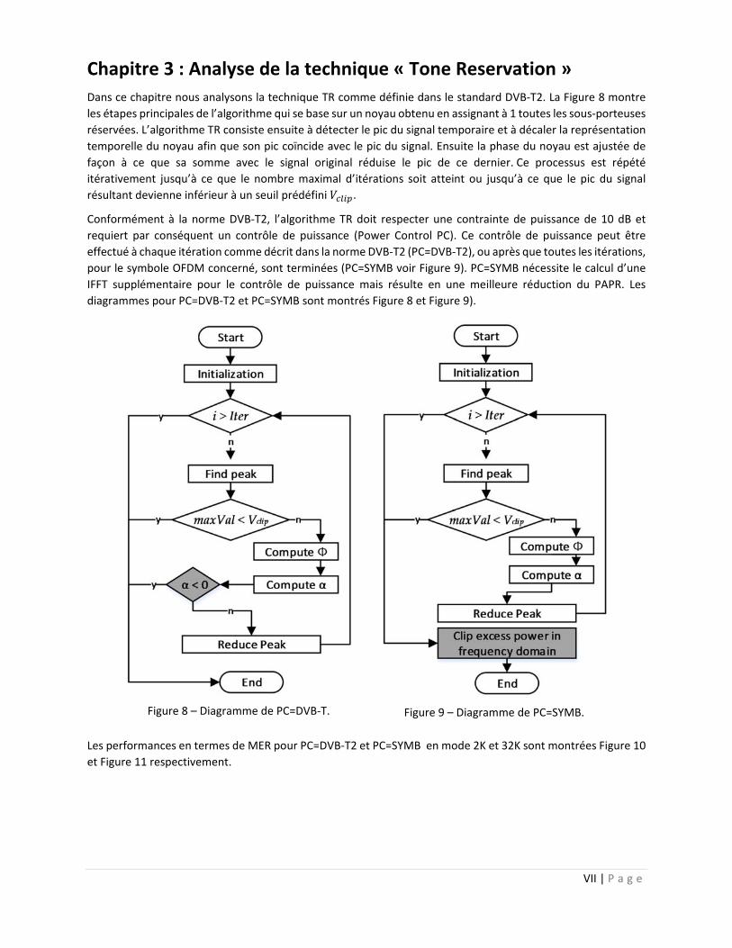
Dans ce chapitre nous analysons la technique TR comme définie dans le standard DVB‐T2. La Figure 8 montre
les étapes principales de l’algorithme qui se base sur un noyau obtenu en assignant à 1 toutes les sous‐porteuses
réservées. L’algorithme TR consiste ensuite à détecter le pic du signal temporaire et à décaler la représentation
temporelle du noyau afin que son pic coïncide avec le pic du signal. Ensuite la phase du noyau est ajustée de
façon à ce que sa somme avec le signal original réduise le pic de ce dernier. Ce processus est répété
itérativement jusqu’à ce que le nombre maximal d’itérations soit atteint ou jusqu’à ce que le pic du signal
résultant devienne inférieur à un seuil prédéfini .
Conformément à la norme DVB‐T2, l’algorithme TR doit respecter une contrainte de puissance de 10 dB et
requiert par conséquent un contrôle de puissance (Power Control PC). Ce contrôle de puissance peut être
effectué à chaque itération comme décrit dans la norme DVB‐T2 (PC=DVB‐T2), ou après que toutes les itérations,
pour le symbole OFDM concerné, sont terminées (PC=SYMB voir Figure 9). PC=SYMB nécessite le calcul d’une
IFFT supplémentaire pour le contrôle de puissance mais résulte en une meilleure réduction du PAPR. Les
diagrammes pour PC=DVB‐T2 et PC=SYMB sont montrés Figure 8 et Figure 9).
Figure 8 – Diagramme de PC=DVB‐T.
Figure 9 – Diagramme de PC=SYMB.
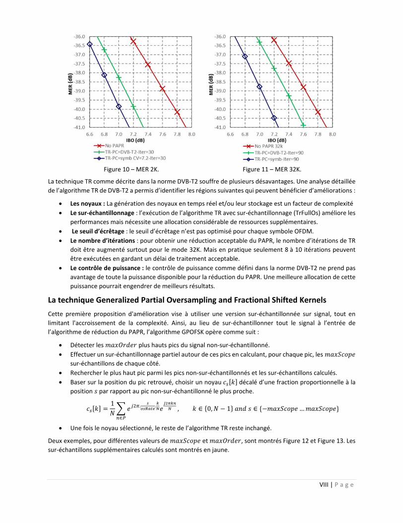
Les performances en termes de MER pour PC=DVB‐T2 et PC=SYMB en mode 2K et 32K sont montrées Figure 10
et Figure 11 respectivement.
VIII | P a g e
Figure 10 – MER 2K.
Figure 11 – MER 32K.
La technique TR comme décrite dans la norme DVB‐T2 souffre de plusieurs désavantages. Une analyse détaillée
de l’algorithme TR de DVB‐T2 a permis d’identifier les régions suivantes qui peuvent bénéficier d’améliorations :
Les noyaux : La génération des noyaux en temps réel et/ou leur stockage est un facteur de complexité
Le sur‐échantillonnage : l’exécution de l’algorithme TR avec sur‐échantillonnage (TrFullOs) améliore les
performances mais nécessite une allocation considérable de ressources supplémentaires.
Le seuil d’écrêtage : le seuil d’écrêtage n’est pas optimisé pour chaque symbole OFDM.
Le nombre d’itérations : pour obtenir une réduction acceptable du PAPR, le nombre d’itérations de TR
doit être augmenté surtout pour le mode 32K. Mais en pratique seulement 8 à 10 itérations peuvent
être exécutées en gardant un délai de traitement acceptable.
Le contrôle de puissance : le contrôle de puissance comme défini dans la norme DVB‐T2 ne prend pas
avantage de toute la puissance disponible pour la réduction du PAPR. Une meilleure allocation de cette
puissance pourrait engendrer de meilleurs résultats.
La technique Generalized Partial Oversampling and Fractional Shifted Kernels
Cette première proposition d'amélioration vise à utiliser une version sur‐échantillonnée sur signal, tout en
limitant l'accroissement de la complexité. Ainsi, au lieu de sur‐échantillonner tout le signal à l’entrée de
l’algorithme de réduction du PAPR, l’algorithme GPOFSK opère comme suit :
Détecter les plus hauts pics du signal non‐sur‐échantillonné.
Effectuer un sur‐échantillonnage partiel autour de ces pics en calculant, pour chaque pic, les
sur‐échantillons de chaque côté.
Rechercher le plus haut pic parmi les pics non‐sur‐échantillonnés et les sur‐échantillons calculés.
Baser sur la position du pic retrouvé, choisir un noyau décalé d’une fraction proportionnelle à la
position par rapport au pic non‐sur‐échantillonné le plus proche.
1 . .
∈
, ∈ 0, 1 ∈ …
Une fois le noyau sélectionné, le reste de l’algorithme TR reste inchangé.
Deux exemples, pour différentes valeurs de et , sont montrés Figure 12 et Figure 13. Les
sur‐échantillons supplémentaires calculés sont montrés en jaune.

IX | P a g e
Figure 12 – GPOFSK avec 2 et 3.
Figure 13 – GPOFSK avec 3 et 1.
L’algorithme GPOFSK est équivalent à :
L’algorithme TR, si 1 et 0 L’algorithme TrFullOs, si et 3
Le diagramme de GPOFSK est montré Figure 14. Les étapes représentées en gris montrent les différences avec
l’algorithme TR.
Figure 14 – Diagramme de GPOFSK.
X | P a g e
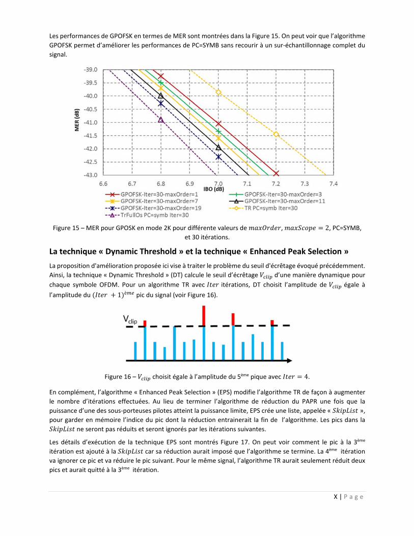
Les performances de GPOFSK en termes de MER sont montrées dans la Figure 15. On peut voir que l’algorithme
GPOFSK permet d’améliorer les performances de PC=SYMB sans recourir à un sur‐échantillonnage complet du
signal.
Figure 15 – MER pour GPOSK en mode 2K pour différente valeurs de , 2, PC=SYMB,
et 30 itérations.
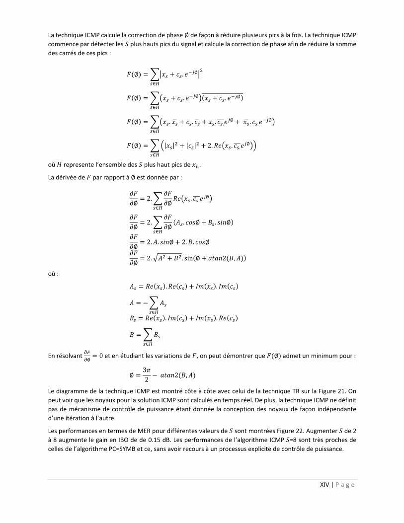
La technique « Dynamic Threshold » et la technique « Enhanced Peak Selection »
La proposition d'amélioration proposée ici vise à traiter le problème du seuil d'écrêtage évoqué précédemment.
Ainsi, la technique « Dynamic Threshold » (DT) calcule le seuil d’écrêtage d’une manière dynamique pour
chaque symbole OFDM. Pour un algorithme TR avec itérations, DT choisit l’amplitude de égale à
l’amplitude du 1 è pic du signal (voir Figure 16).
Figure 16 – choisit égale à l’amplitude du 5ème pique avec 4.
En complément, l’algorithme « Enhanced Peak Selection » (EPS) modifie l’algorithme TR de façon à augmenter
le nombre d’itérations effectuées. Au lieu de terminer l’algorithme de réduction du PAPR une fois que la
puissance d’une des sous‐porteuses pilotes atteint la puissance limite, EPS crée une liste, appelée « »,
pour garder en mémoire l’indice du pic dont la réduction entrainerait la fin de l’algorithme. Les pics dans la
ne seront pas réduits et seront ignorés par les itérations suivantes.
Les détails d’exécution de la technique EPS sont montrés Figure 17. On peut voir comment le pic à la 3ème
itération est ajouté à la car sa réduction aurait imposé que l’algorithme se termine. La 4ème itération
va ignorer ce pic et va réduire le pic suivant. Pour le même signal, l’algorithme TR aurait seulement réduit deux
pics et aurait quitté à la 3ème itération.

XI | P a g e
Itération Domaine Temporel Domaine Fréquentiel
1ère
2ème
3ème
4ème
Figure 17 – Détails des itérations de la technique EPS.
Le nombre d’itérations exécutées de la technique EPS combinée avec DT est montré dans la Table 2. À comparer
avec PC=DVB‐T2, on peut voir que EPS DT permet d’exécuter un nombre supérieur d’itérations.
Table 2 – Puissance utilisée et nombre d’itérations effectuées en mode 32K.
32k mode DVB_T2 EPS‐DT EPS‐DT EPS_DT SYMB
Vclip / VclipRef 7.2dB 120 120 120 7.2dB
Max. Iterations 90 30 60 90 90
Avg. # of iterations 9.6 29.3 56.5 79.4 90
Avg. Pilot power usage 20.5% 14.6% 16.7% 17.9% 51.2%
Le diagramme des techniques EPS et DT combinées est montré Figure 18. Les étapes représentées en gris
montrent les différences avec l’algorithme TR tel que défini dans la norme DVB‐T2.

XII | P a g e
Figure 18 – Diagramme d’EPS combinée DT.
Les performances en termes de MER sont montrées Figure 19. La technique EPS‐DT permet d’augmenter le gain
en MER de PC=DVB‐T2 de 0.15 dB.
Figure 19 – MER pour EPS combinée avec DT en mode 32K.

XIII | P a g e
Chapitre 4 : La technique « Individual Carrier Multiple Peaks »
Le contrôle de puissance pour l’algorithme TR de la norme DVB‐T2 est conçu pour éviter l’utilisation d’une IFFT
additionnelle. Cela rend son implémentation moins complexe mais conduit également à ne pas utiliser une
grande partie de la puissance disponible pour les pilotes. Dans ce chapitre on propose une nouvelle solution qui
permet une meilleure utilisation de la puissance disponible pour tous les pilotes.
La technique « Individual Carrier Multiple Peaks »
La technique « Individual Carrier Multiple Peaks » ICMP, définit un noyau différent pour chaque itération
comme suit :
0
où représente la position du pilote correspondant à l’itération courante. La relation entre les noyaux et les
itérations est montrée Figure 20.
La représentation temporelle des noyaux est donnée par :
. ∅ .. .
, ∈ 0, 1
Les noyaux, dans le domaine temporel, sont caractérisés par:
une amplitude constante égale à , et
un changement de phase entre deux échantillons successifs égale à.
.
Pour la technique TR de la norme DVB‐T2, la génération d’un noyau requiert le calcul d’une IFFT. Tandis que
pour la technique IMCP, les échantillons d’un même noyau peuvent être générés par un simple changement de
phase :
. ∅ .. .
. ∅ .. .
..
1st iteration 2nd iteration
3rd iteration 4th iteration
Figure 20 – Relation entre les itérations et les noyaux ICMP.
XIV | P a g e
La technique ICMP calcule la correction de phase ∅ de façon à réduire plusieurs pics à la fois. La technique ICMP
commence par détecter les plus hauts pics du signal et calcule la correction de phase afin de réduire la somme
des carrés de ces pics :
∅ . ∅
∈
∅ . ∅ . ∅
∈
∅ . . . .∅ . .
∅
∈
∅ | | | | 2. . .∅
∈
où represente l’ensemble des plus haut pics de .
La dérivée de par rapport à ∅ est donnée par :
∅2.
∅. .
∅
∈
∅2.
∅. ∅ . ∅
∈
∅2. . ∅ 2. . ∅
∅2. . sin ∅ 2 ,
où :
. .
∈
. .
∈
En résolvant ∅
0 et en étudiant les variations de , on peut démontrer que ∅ admet un minimum pour :
∅
32
2 ,
Le diagramme de la technique ICMP est montré côte à côte avec celui de la technique TR sur la Figure 21. On
peut voir que les noyaux pour la solution ICMP sont calculés en temps réel. De plus, la technique ICMP ne définit
pas de mécanisme de contrôle de puissance étant donnée la conception des noyaux de façon indépendante
d’une itération à l’autre.
Les performances en termes de MER pour différentes valeurs de sont montrées Figure 22. Augmenter de 2
à 8 augmente le gain en IBO de de 0.15 dB. Les performances de l’algorithme ICMP =8 sont très proches de
celles de l’algorithme PC=SYMB et ce, sans avoir recours à un processus explicite de contrôle de puissance.

XV | P a g e
Figure 21 – Diagramme de la technique ICMP et de TR PC=DVB‐T2.
Figure 22 – MER pour ICMP pour différentes valeurs de en mode 2K.
La technique « Grouped ICMP »
Le nombre d’itérations exécutées par la technique ICMP doit être égal au nombre de sous‐porteuses réservées.
Pour le mode 2K, 18 itérations seront nécessaires. Cela devient problématique pour des tailles supérieures

XVI | P a g e
d’IFFT. Par exemple, pour le mode 32K, la technique ICMP doit exécuter 288 itérations ce qui causerait un long
délai de traitement vu que chaque itération doit parcourir tout le signal à la recherche des plus hauts pics.
La technique Grouped ICMP (GICMP) modifie l’algorithme ICMP en divisant les pilotes en groupes. Une seule
recherche de pics est exécutée par groupe. Le reste des étapes de l’algorithme ICMP pour un même groupe
restent inchangées. Les étapes d’un même groupe sont décorrélées, et peuvent être exécutées en parallèle pour
réduire le délai de traitement. Le diagramme de l’algorithme GICMP est montré Figure 23.
Figure 23 – Diagramme de la technique ICMP.
La Table 3 montre le nombre de recherches de pics nécessaires pour différentes tailles de groupes. Pour =288,
le nombre est le même pour les deux algorithmes GICMP et ICMP
Table 3 – Différentes configurations possibles pour GICMP en mode 32K.
Group count ( )
Pilots per group
Peak search operations required
Kernels that can be generated in parallel
1 288 1 288
2 144 2 144
4 72 4 72
8 36 8 36
16 18 16 18
288 (No Grouping) 1 288 1
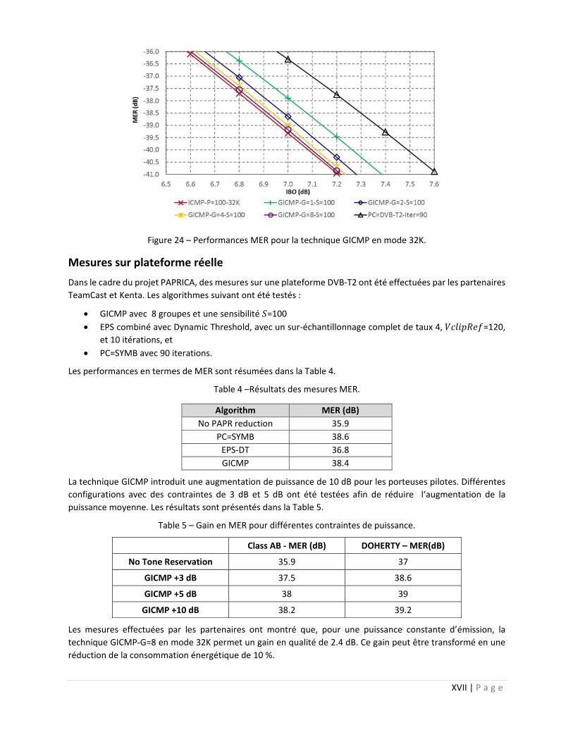
La Figure 24 montre les performances en MER pour l’algorithme GICMP en mode 32K. Avec seulement un groupe
(une seule détection de pics exécutée) l’algorithme GICMP permet un gain en IBO de 0.23 dB par rapport à
l’algorithme PC=DVB‐T2 (90 itérations allouées et 9 itérations et détections de pics exécutées en moyenne).
Pour =8, les performances de la technique GICMP sont presque les mêmes que celles de la technique ICMP.
L’algorithme GICMP‐G=8 permet un gain de 0.3 dB par rapport la solution PC=DVB‐T2.
Initialization
Compute H
End
Compute φ1
Start
g > G
Reduce Peak
y
n
Generate Kernel
Add Kernels
Compute φ2
Generate Kernel
Compute φGS
Generate Kernel
XVII | P a g e
Figure 24 – Performances MER pour la technique GICMP en mode 32K.
Mesures sur plateforme réelle
Dans le cadre du projet PAPRICA, des mesures sur une plateforme DVB‐T2 ont été effectuées par les partenaires
TeamCast et Kenta. Les algorithmes suivant ont été testés :
GICMP avec 8 groupes et une sensibilité =100
EPS combiné avec Dynamic Threshold, avec un sur‐échantillonnage complet de taux 4, =120,
et 10 itérations, et
PC=SYMB avec 90 iterations.
Les performances en termes de MER sont résumées dans la Table 4.
Table 4 –Résultats des mesures MER.
Algorithm MER (dB)
No PAPR reduction 35.9
PC=SYMB 38.6
EPS‐DT 36.8
GICMP 38.4
La technique GICMP introduit une augmentation de puissance de 10 dB pour les porteuses pilotes. Différentes
configurations avec des contraintes de 3 dB et 5 dB ont été testées afin de réduire l‘augmentation de la
puissance moyenne. Les résultats sont présentés dans la Table 5.
Table 5 – Gain en MER pour différentes contraintes de puissance.
Class AB ‐ MER (dB) DOHERTY – MER(dB)
No Tone Reservation 35.9 37
GICMP +3 dB 37.5 38.6
GICMP +5 dB 38 39
GICMP +10 dB 38.2 39.2
Les mesures effectuées par les partenaires ont montré que, pour une puissance constante d’émission, la
technique GICMP‐G=8 en mode 32K permet un gain en qualité de 2.4 dB. Ce gain peut être transformé en une
réduction de la consommation énergétique de 10 %.

XVIII | P a g e
Chapitre 5 : Techniques conjointes de réduction du PAPR et
d’estimation du canal
La technique TR réserve à peu près 1 % des sous‐porteuses disponibles pour la réduction du PAPR. La norme
DVB‐T2 alloue aussi un certain nombre de pilotes pour l’estimation du canal au sein du récepteur. Les techniques
conjointes de réduction du PAPR et d’estimation du canal utilisent les mêmes sous‐porteuses pour les deux
fonctions. Ceci permet d’augmenter l’efficacité spectrale.
La technique CEPR
La technique « Channel Estimation and PAPR Reduction » CEPR se base sur une relation géométrique entre les
pilotes réservés :
∀ ∈ 0, … , 2 avec
La relation géométrique est montrée Figure 25. Cette relation est définie par trois paramètres:
: le « boost factor », ∈ R
: la phase initiale ou la correction de phase, ∈ 0,2π
: l’incrément de phase, ∈ 0,2π
Figure 25 – Loi géométrique pour les pilotes de CEPR.
Pour la réduction du PAPR à l’émetteur, l’algorithme CEPR exécute une recherche exhaustive pour trouver la
meilleure séquence qui vérifie la relation géométrique et réduit le PAPR. Le récepteur ne connait pas les valeurs
choisies par l’émetteur, mais utilise la relation géométrique pour calculer une estimation des valeurs transmises.
Cette estimation est ensuite utilisée comme séquence de référence pour estimer les coefficients du canal. La
Figure 26 montre le schéma bloc de la technique CEPR.
Pour limiter le nombre de séquences à tester par l’émetteur. Les valeurs et sont choisies parmi des
ensembles de valeurs discrètes avec des étapesμ et μ respectivement.
: variable in discrete domain
: variable in discrete domain
C0
C2
C1: fixed value
C0= ejCk= ej(+k)

XIX | P a g e
Figure 26 – Schéma bloc de la technique CEPR.
La technique F‐CEPR
La technique CEPR souffre d’une complexité d’implémentation élevée. En fait, l’algorithme de recherche
exhaustive de la solution CEPR calcule une IFFT pour chaque séquence possible. Pour éviter cela on propose la
technique Fast‐CEPR (F‐CEPR) qui se base sur une distribution uniforme des pilotes. L’ensemble des pilotes pour
la solution F‐CEPR est donné par :
, 0
La version temporelle du noyau est donnée par :
λM
√ 0
0
L’algorithme F‐CEPR recherche le plus haut pic du signal temporel et réduit en calculant et comme suit :
2.
et
D
où représente la position du pic détecté et | représente la fonction de décision discrète avec une
étape .
La technique FS‐CEPR
La technique F‐CEPR réduit seulement un seul pic. Un nombre supérieur de pics peut être réduit en superposant
plusieurs séquences F‐CEPR. Ainsi, la technique Fast Shifted CEPR (FS‐CEPR) superpose sequences F‐CEPR,
ces « sous‐séquences » F‐CEPR sont décalées l’une par rapport à l’autre de positions.
XX | P a g e
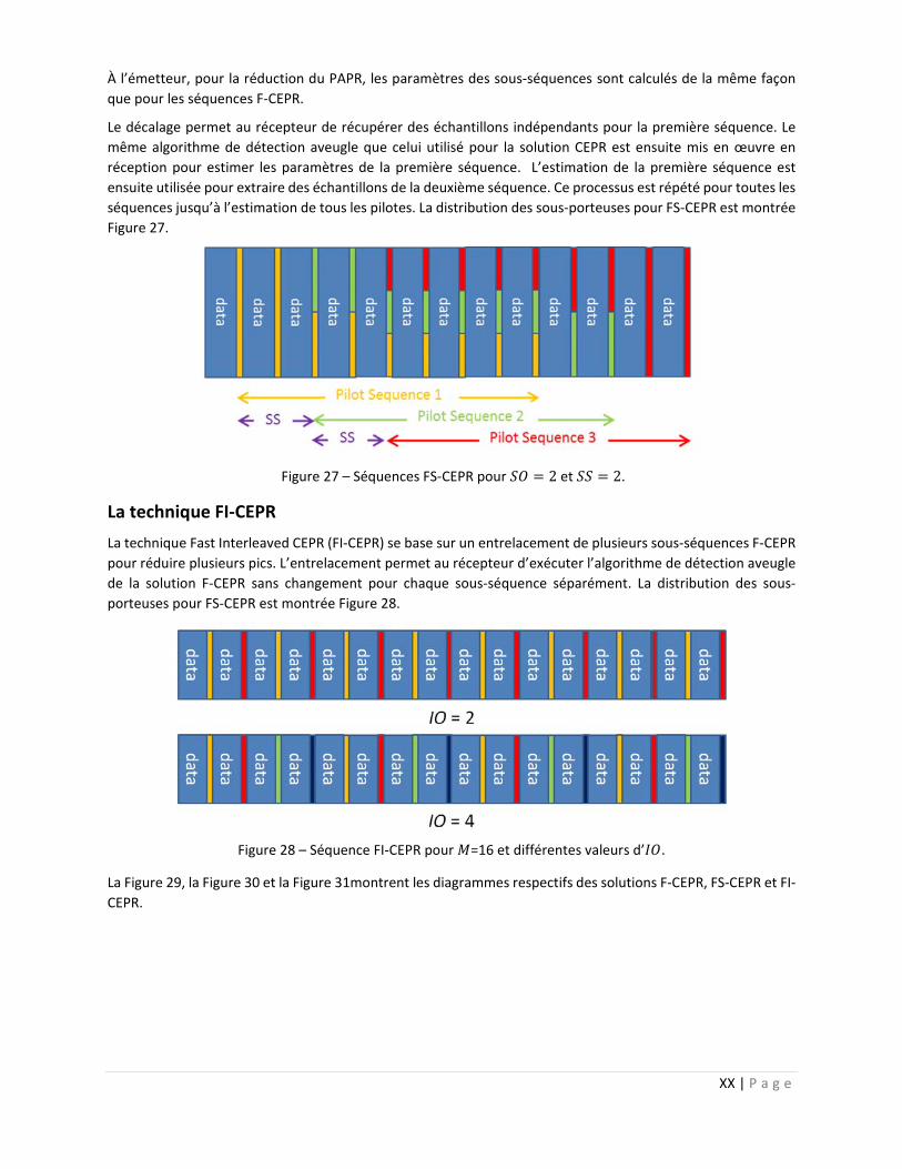
À l’émetteur, pour la réduction du PAPR, les paramètres des sous‐séquences sont calculés de la même façon
que pour les séquences F‐CEPR.
Le décalage permet au récepteur de récupérer des échantillons indépendants pour la première séquence. Le
même algorithme de détection aveugle que celui utilisé pour la solution CEPR est ensuite mis en œuvre en
réception pour estimer les paramètres de la première séquence. L’estimation de la première séquence est
ensuite utilisée pour extraire des échantillons de la deuxième séquence. Ce processus est répété pour toutes les
séquences jusqu’à l’estimation de tous les pilotes. La distribution des sous‐porteuses pour FS‐CEPR est montrée
Figure 27.
Figure 27 – Séquences FS‐CEPR pour 2 et 2.
La technique FI‐CEPR
La technique Fast Interleaved CEPR (FI‐CEPR) se base sur un entrelacement de plusieurs sous‐séquences F‐CEPR
pour réduire plusieurs pics. L’entrelacement permet au récepteur d’exécuter l’algorithme de détection aveugle
de la solution F‐CEPR sans changement pour chaque sous‐séquence séparément. La distribution des sous‐
porteuses pour FS‐CEPR est montrée Figure 28.
Figure 28 – Séquence FI‐CEPR pour =16 et différentes valeurs d’ .
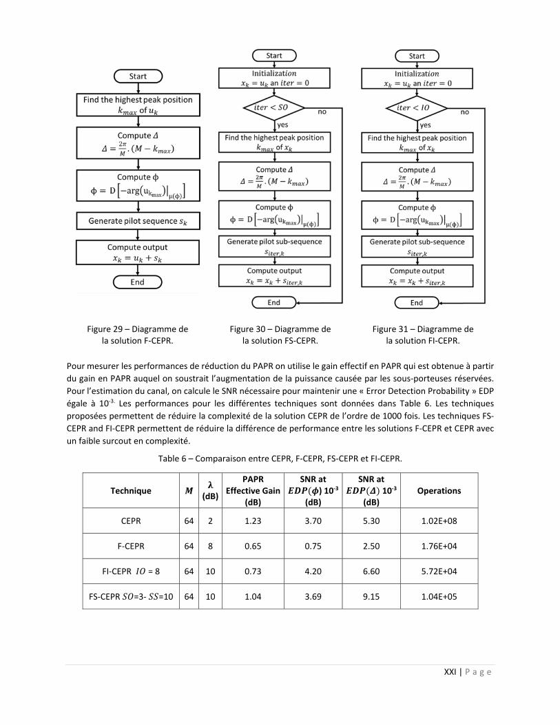
La Figure 29, la Figure 30 et la Figure 31montrent les diagrammes respectifs des solutions F‐CEPR, FS‐CEPR et FI‐
CEPR.
XXI | P a g e
Figure 29 – Diagramme de la solution F‐CEPR.
Figure 30 – Diagramme de la solution FS‐CEPR.
Figure 31 – Diagramme de la solution FI‐CEPR.
Pour mesurer les performances de réduction du PAPR on utilise le gain effectif en PAPR qui est obtenue à partir
du gain en PAPR auquel on soustrait l’augmentation de la puissance causée par les sous‐porteuses réservées.
Pour l’estimation du canal, on calcule le SNR nécessaire pour maintenir une « Error Detection Probability » EDP
égale à 10‐3. Les performances pour les différentes techniques sont données dans Table 6. Les techniques
proposées permettent de réduire la complexité de la solution CEPR de l’ordre de 1000 fois. Les techniques FS‐
CEPR and FI‐CEPR permettent de réduire la différence de performance entre les solutions F‐CEPR et CEPR avec
un faible surcout en complexité.
Table 6 – Comparaison entre CEPR, F‐CEPR, FS‐CEPR et FI‐CEPR.
Technique
(dB)
PAPR Effective Gain
(dB)
SNR at ) 10‐3
(dB)
SNR at 10‐3
(dB) Operations
CEPR 64 2 1.23 3.70 5.30 1.02E+08
F‐CEPR 64 8 0.65 0.75 2.50 1.76E+04
FI‐CEPR = 8 64 10 0.73 4.20 6.60 5.72E+04
FS‐CEPR =3‐ =10 64 10 1.04 3.69 9.15 1.04E+05

22 | P a g e
Conclusion
L’objectif de cette thèse est d’optimiser l’efficacité énergétique des systèmes de diffusion numérique. Le HPA
est responsable d’au moins 50% de l’énergie consommée par un système typique de diffusion numérique, cette
consommation pouvant atteindre quelques dizaines de kWatts.
Au début de ce manuscrit, on a commencé par introduire la modulation OFDM qui est largement utilisée dans
les systèmes modernes de télécommunications. Puis on a expliqué comment les signaux OFDM, qui sont
caractérisés par un taux élevé de fluctuation de puissance, ne permettent pas d’utiliser les HPAs dans leur région
optimale de rendement énergétique. On a alors introduit la métrique PAPR, utilisée pour quantifier les
fluctuations de puissance, et discuté de plusieurs méthodes de réduction du PAPR proposées dans la littérature.
En particulier on a présenté la technique TR qui a été adoptée par le standard DVB‐T2. Ce standard et son
prédécesseur DVB‐T sont largement déployés en Europe, Afrique et Asie.
Comme détaillé dans notre étude, la technique TR souffre de plusieurs désavantages. On a analysé cette solution
en détails pour expliquer en quoi cette technique n’offre par un bon compromis performance‐complexité. Cette
analyse a permis d’identifier plusieurs possibilités d’améliorations qui ont été à la base de la proposition de
plusieurs algorithmes novateurs qui permettent d’accroître les performances et/ou réduire la complexité de la
technique TR.
En synthèse de l'ensemble de l'étude, les algorithmes proposés sont comparés dans la Table 7 et peuvent être
groupés en deux catégories. La première garde la même définition du noyau que la solution TR de la norme DVB‐
T2. Cette catégorie inclut : (1) la technique « General Partial Oversampling and Fractional Shifted Kernels »
(GPOFSK) technique qui tire avantage de la précision apportée par le sur‐échantillonnage en ne sur‐
échantillonnant que partiellement le signal, (2) La technique Enhanced Peak Selection (EPS) permet d’éviter la
réduction des pics qui entraîne l’arrêt prématuré de l’algorithme, et ce en identifiant ces pics et en les ajoutant
à une « SkipList », et (3) la technique DT effectue un calcul dynamique du seuil de réduction afin d’optimiser ce
seuil pour chaque symbole OFDM.
Table 7 – Comparaison.
PC=DVB‐T2 PC=SYMB POFSK EPS‐DT GICMP
Real‐time kernel generation NO (‐) NO (‐) NO (‐) NO (‐) YES (+)
Memory for kernel storage YES (‐) YES (‐) YES (‐) YES (‐) NO (+)
Power Control (PC) required YES (‐) YES (‐) YES (‐) YES (‐) NO (+)
IFFT required for PC NO (+) YES (‐) YES (‐) NO (+) NO (+)
Compatible with DVB‐T2 YES (+) YES (+) YES (+) YES (+) YES (+)
Parallelization possible NO (‐) NO (‐) NO (‐) NO (‐) YES (+)
Efficient use of pilot power NO (‐) YES (+) YES (+) YES (+) YES (+)
Acceptable performance with 8‐10 peak search operations in 32K
mode NO (‐) YES (+) YES (+) YES (+) YES (+)
La deuxième catégorie comporte deux techniques qui changent la définition du noyau de la solution TR. La
technique ICMP définit, pour chaque itération, un noyau unique et simple à calculer en temps réel. La phase de
ce noyau est ajustée avec une correction de phase calculée de façon à réduire plusieurs pics à la fois. Le nombre
d’itérations exécutées par la solution ICMP est faible pour des petites tailles d’IFFT, mais ce nombre augmente
considérablement avec la taille de l’IFFT pour atteindre 298 itérations en mode 32K. La technique Grouped ICMP
(GICMP) permet de grouper plusieurs itérations ICMP ensemble. Les itérations d’un même groupe peuvent être
exécutées en parallèle ce qui permet de réduire considérablement le délai de traitement tout en gardant de

23 | P a g e
bonnes performances. La table 7 résume les principales caractéristiques et avantages des différentes solutions
étudiées.
La technique GICMP avec 8 groupes a été testée par les partenaires dans le projet PAPRICA sur une plateforme
de diffusion DVB‐T2. Les mesures ont montré que cette technique apporte un gain en termes de MER de 2.4 dB.
Ce gain en qualité peut être transformé en une réduction de 10 % de la puissance consommée.
Dans la deuxième partie de cette thèse, on a étudié la technique conjointe de réduction du PAPR et d’estimation
du canal CEPR. Cette technique se base sur une recherche exhaustive à l’émetteur. Pour éviter le coût élevé en
complexité on a proposé trois nouvelles techniques :
La technique Fast F‐CEPR se base sur une distribution uniforme des pilotes et utilise les propriétés de la
représentation temporelle des pilotes pour réduire un pic sans avoir à effectuer une recherche
exhaustive.
La technique Fast Shifted CEPR permet d’augmenter les performances de la solution F‐CEPR en
superposant plusieurs séquences F‐CEPR afin de réduire plusieurs pics.
La technique Fast‐Interleaved CEPR (FI‐CEPR), comme FS‐CEPR, réduit plusieurs pics et ce en entrelaçant
plusieurs séquences F‐CEPR.
Les trois techniques proposées permettent au récepteur d’utiliser la même logique de détection aveugle utilisée
par la solution CEPR pour l’estimation de la réponse du canal de transmission.


25 | P a g e
General Introduction
Since the invention of the television (TV) in the early 20th century, its market has been constantly growing. The
TV industry generated over 407 billion euros of revenue in 2014 and is projected to generate 474.6 billion euros
in 2018 [1]. Today, there are more than 1,554 million TV households out of which 1,055 million use digital TV
(including Terrestrial TV, Cable TV, satellite TV and IPTV). For the period between 2010 and 2014, the penetration
rate of Digital TV increased from 40.5 percent to 67.2 percent [2].
This thesis aims at optimizing the energy efficiency of digital broadcasting systems in general and of the second
generation of the Digital Video Broadcasting Terrestrial (DVB‐T2) standard in particular. The first generation DVB
standard was released by the European DVB consortium in the early 90s, and DVB‐T2 followed in 2008. DVB‐T
and DVB‐T2 have been trialed, adopted or deployed in more than 150 countries worldwide, mainly in Europe,
Asia (except China, Japan, Philippines and Sri Lanka) and Australia.
DVB‐T2, similar to many modern telecommunication systems (such as ADSL, Wi‐MAX, Wi‐Fi, DVB), adopted the
Orthogonal Frequency Division Multiplexing (OFDM) technique for its robustness, high transmission rates,
mobility and bandwidth efficiency. However, OFDM signals are characterized by high power fluctuations, which
cause distortions at the output of nonlinear components of the transmission chain.
The High Power Amplifier (HPA) is the main source of nonlinearities in a typical transmission system and has
been shown to consume 55‐60 percent of the total macro base station power in 4G Long Term Evolution (LTE)
cellular networks according to the Energy Aware Radio and NeTwork Technologies (EARTH) project. The
percentage of HPA power consumption is even higher in digital terrestrial TV networks where transmission
power can reach 100 dBm (compared to 43 dBm for a 4G LTE macro base station).
The power fluctuations of OFDM signals prevent the radio frequency designer to feed the signal at the optimal
point of the HPA specifications. Moreover, these fluctuations lead to in‐band and Out‐Of‐Band (OOB) distortions
generating degraded Bit Error Rate (BER) performance and high adjacent channel interference respectively. This
highlights the vast potential for energy savings by reducing the amount of signal fluctuations at the input of the
HPA. The Peak to Average Power Ratio (PAPR) metric has been widely used to quantify power fluctuations. Many
PAPR reduction techniques have been proposed in the literature. The DVB‐T2 standard adopted two PAPR
reduction techniques: the Active Constellation Extension (ACE) and the Tone Reservation (TR) technique.
The ACE technique modifies the constellation points of the signal. The new constellation points are selected in
a way to both reduce the PAPR of the transmitted signal and preserve the same Bit Error Rate. ACE suffers from
26 | P a g e
multiple disadvantages: (1) it is not compatible with rotated constellations, which provide additional robustness
when used; (2) its performance drops with large constellations; and (3) its implementation in the DVB‐T2
standard requires two IFFT blocks and one FFT block to be computed sequentially, thus increases the processing
delay caused by ACE.
The TR technique reserves a set of sub‐carriers for PAPR reduction. The TR implementation in DVB‐T2 is based
on a kernel created by setting all the subcarrier values to one. The time domain representation of the kernel has
an impulse‐like shape. TR iteratively reduces the PAPR by reducing one peak at a time. In each iteration the
highest peak is detected, then a copy of the kernel is scaled, circularly shifted and its phase adjusted in such a
way that the kernel’s peak and the signal’s peak coincide with opposite phases. The kernel is then added to the
signal in time domain and the process is repeated until either the number of executed iterations exceeds a
certain limit or the amplitude of the highest peak becomes lower than a predefined threshold. To the best of
our knowledge at the time of writing, the TR algorithm has not been implemented by DVB‐T2 modulator
manufacturers since it does not offer the right performance complexity tradeoff (i.e. the number of iterations
required to achieve reasonable PAPR reduction increases for large IFFT sizes, which translates into a longer
processing delay and requires upgrades to the hardware of current market modulators).
This thesis studies in detail the TR algorithm proposed in the DVB‐T2 standard and proposes multiple novel
techniques based on TR that increase the performance of TR and/or reduce its complexity.
Project PAPRICA
A large part of this thesis is linked to the French regional project Peak to Average Power Ratio Iterative
Compression Algorithm (PAPRICA); a project supported by the Brittany Region. PAPRICA focuses on improving
the power efficiency of DVB‐T2 modulators by proposing new techniques to reduce the PAPR with reasonable
complexity and without generating additional hardware cost. Three partners are involved in the project:
TeamCast Technologies (a manufacturer of DVB modulators), Kenta Electronic (a manufacturer of power
amplifiers) and INSA‐IETR (a research laboratory).
Thesis Organization
This thesis is organized as follows:
Chapter 1 explains the principle of Orthogonal Frequency Division Multiplexing (OFDM) systems, presents an
overview of Digital Terrestrial Television Broadcasting (DTTB) standards and describes the main technological
features of DVB‐T2.
Chapter 2 is dedicated to the Peak to Average Power Ratio (PAPR) problem. It explains the impact of the HPA
nonlinearity on the performance and power consumption. Various PAPR reduction techniques are also discussed
in this chapter, and the two techniques adopted in DVB‐T2, Tone Reservation (TR) and ACE (Active Constellation
Extension), are detailed.
A deep analysis of the TR algorithm adopted in DVB‐T2 is presented in Chapter 3. As a result, multiple
improvement areas are identified. These areas are related to (1) the power constraint imposed by the standard,
(2) the clipping threshold used, (3) the level of oversampling, (4) the algorithm exit conditions and (5) the design
of the kernel. The outcome of this analysis is then used as a basis to propose multiple novel algorithms. Each of
the proposed algorithms provides improvements compared to the DVB‐T2 version in at least one area. The first
group of algorithms introduces changes and enhancements to the TR algorithm adopted in DVB‐T2 TR, but keeps
the same kernel definition. This group includes: the Partial Oversampling and Fractional Shifted Kernels (POFSK)
technique, which is based on a partial oversampling of the signal in order to provide good PAPR reduction
performance without requiring the complete signal to be oversampled; the Dynamic Threshold (DT) technique
which allows better algorithm convergence by dynamically computing the PAPR reduction threshold for every
OFDM symbol; and the Enhanced Peak Selection (EPS) technique, which provides additional PAPR reduction by
choosing the appropriate signal peaks to reduce and the peaks to skip.

27 | P a g e
The second group of algorithms is presented in Chapter 4. This group includes the Individual Carrier Multiple
Peaks (ICMP) technique and the Grouped ICMP (GICMP). ICMP is based on a special kernel definition that
changes from one algorithm iteration to another and uses a different phase calculation approach that reduces
multiple peaks at a time. GICMP is an optimized version of ICMP that allows for the parallelization of iterations
in such a way to reduce the processing delay and the number of algorithm iterations. The implementation details
of GICMP on a real hardware platform are presented along with measurements gathered from a real
transmission system.
Chapter 5 introduces the joint channel estimation and PAPR reduction techniques, which optimizes the
bandwidth by using the same pilots for PAPR reduction and channel estimation. Multiple novel improvements
to the Channel Estimation and PAPR Reduction (CEPR) technique, which is too complex to implement since it
requires an exhaustive search to be used, are proposed: the Fast CEPR (F‐CEPR) avoids the use of costly
exhaustive search, but reduces only one signal peak; the Fast Shifted CEPR (FS‐CEPR) and the Fast Interleave (FI‐
CEPR) rely on shifting and interleaving of multiple F‐CEPR sequences in order to avoid exhaustive search and, at
the same time, reduce multiple signal peaks.
Finally, the main results of this work are summarized in the general conclusion where some prospects are also
drawn.
Publications
Patents:
Mounzer R.; Crussière M.; Hélard J‐F.; Nasser Y., "Procédé et dispositif de transmission d’un signal multi‐
porteuse, programme et signal correspondants", Brevet français publié sous la référence N°1554085
déposée le 6 mai 2015.
List of international communications with proceedings:
Mounzer R.; M.; Nasser Y.; Hélard J.‐F., “Tone Reservation based PAPR Reduction Technique with
Individual Carrier Power Allocation for Multiple Peaks Reduction,” Proceedings of IEEE 81st Vehicular
Technology Conference (VTC Spring), May 2015, Glasgow, Scotland.
Mounzer R.; Crussière M.; Nasser Y.; Hélard J.‐F., “Power Control Optimization for Tone Reservation
based PAPR reduction algorithms” Proceedings of IEEE International Symposium on Personal Indoor and
Mobile Radio Communications (PIMRC2014), Sep 2014, Washington, United States of America (USA).
Mounzer R.; Nasser Y.; Hélard J.‐F., "Design of interleaved sequences for joint channel estimation and
PAPR reduction," 2013 Third International Conference on Communications and Information Technology
(ICCIT), pp.235‐240, 19‐21 June 2013.
Mounzer R.; Nasser Y.; Hélard J.‐F., "A low complexity scheme for joint channel estimation and PAPR
reduction technique,” 35th IEEE Sarnoff Symposium (SARNOFF), pp.1,6, 21‐22 May 2012.
Rosati S.; Candreva E.A.; Nasser Y.; Yun S.R.; Corazza G.E.; Mounzer R.; Hélard J.‐F.; Mourad A., "PAPR
reduction techniques for the next generation of mobile broadcasting," 19th International Conference on
Telecommunications (ICT), pp.1‐6, 23‐25 April 2012


29 | P a g e
OFDM and Digital
Video Broadcasting
In this chapter, a top down approach is adopted to introduce all the technological concepts required for a good
understanding of this manuscript. Orthogonal Frequency Division Multiplexing (OFDM) is firstly introduced in
paragraph 1.1. OFDM has been adopted by multiple Digital Terrestrial Television Broadcasting (DTTB) systems.
A quick overview of these systems is then given in paragraph 1.2. This study is mainly based on the European
DTTB of second generation maintained by European Telecommunications Standards Institute (ETSI) and named
Digital Video Broadcasting for Terrestrial version 2 (DVB‐T2). In paragraph 1.3, the main technical innovations
that make DVB‐T2 a more modern version than its predecessor DVB‐T are presented.
1.1 OrthogonalFrequencyMultiplexingSystems
The need for high data rates for wireless and mobile users has been increasing over the past decade.
Transmission over radio channel suffers from multipath, which can result in long echoes. At the receiver, these
echoes cause Inter Symbol Interference (ISI) which is considered as the main cause of harmful detection. OFDM
is a multi‐carrier system that was designed to combat ISI. In this section, ISI is discussed. The principle behind
OFDM is then explained: how OFDM divides the spectrum into orthogonal sub‐channels over which the encoded
data is transmitted in parallel.
1.1.1 HistoryofOFDM
The concept of multicarrier transmission was introduced in 1960s [3] [4], by Chang. In 1971 Weinstein and Ebert
[5] proposed a simplified implementation by using a technique based on the Fourier Transform. Hiroskai [6]
further developed this technique in 1981.
OFDM stayed unknown to the scientific and engineering communities until 1985 when Cimini [7] pointed that
using guard intervals with an OFDM system is well suited for mobile radio. Inspired by Cimini’s paper, France’s
Centre for the Study of Television broadcasting and Telecommunication (CCETT acronym for Centre Commun

30 | P a g e
d'Etudes de Télévision et Télécommunications) proposed, in 1987, a digital broadcasting system based on OFDM
to be used with mobile receivers [8].
An OFDM system was standardized in 1993 after being considered by the European Digital Audio Broadcasting
(DAB) project. The standard is published by ETSI and carries document number EN 300 401 and the final draft
was released in 2006 [9].
The choice of the guard interval length was major design challenge for OFDM based systems. Severe signal
degradation takes place when the guard interval is shorter that the echoed signals [10]. In 1990, The German
Postal, Telegraph and Telephone Company in a dual project with Bosh conducted extended measurement of the
mobile radio channel which resulted in specification for the choice of system parameters for the all DAB
transmission modes.
At that time, DQPSK modulation was chosen the Digital Audio Broadcasting Applications since no channel
estimation methods were available for OFDM. Hence DQPSK was used along with conventional coding in DAB.
But, in 1991 Hoeher [11] used Wiener filtering to perform channel estimation and showed that when combined
with coherent coding it outperformed DQPSK. Hoeher’s ideas were incorporated in the Digital Video
Broadcasting ‐ Terrestrial (DVB‐T) standard that was first published in 1997 [12]. Also in 1991, Hélard and Le
Floch proposed a way to combine coherent demodulation with Trellis codes to enhance the spectral efficiency
of DVB‐T systems [13] .
The DAB standard is considered as the pioneer in OFDM systems. In fact DVB‐T adopted many aspects of DAB:
the choice of symbol length, the transmission modes and channel coding.
IEEE 802.11a [14] and HIPERLAN/2 standards, released in 1999 and 2000 respectively, adopted transmission
techniques based on OFDM. These standard were developed by two different working groups both established
in 1997, the first by IEEE and the second by ETSI. These groups carried extensive discussions which led to
harmonized parameters, channel coding and modulation for OFDM.
Table 1.1 displays a list of standards that adopted OFDM. It has been used in wired systems (such as ADSL, HDSL
and VDSL), in broadcasting systems such as (DAB, DVB‐T and DVB‐T2), by many of the 802.11 Wi‐Fi family
standards and in modern 4G cellular networks.
Table 1.1 – Major standards using OFDM.
Standard Year
ANSI ADSL standard [15] 1991
ANSI HDSL standard [16] 1994
ETSI DAB standard [17] 1995
ETSI WLAN standard [18] 1996
ETSI DVB‐T standard [19] 1997
ANSI VDSL and ETSI VDSL standards [20] [21] 1998
ETSI BRAN standard [22] 1998
IEEE 802.11a WLAN standard [14] 1999
IEEE 802.11g WLAN standard [23] 2002
ETSI DVB‐H standard [24] 2004
IEEE 802.16 WMAN standard [25] 2004
Candidate for IEEE 802.11n standard for next generation WLAN [26] 2004
Candidate for IEEE 802.15.3a standard for WPAN (using MB‐OFDM) [27] 2004
Candidate for 4G standards in China, Japan and South Korea (CJK) [28] 2005
ETSI DVB‐T2 standard 2008

31 | P a g e
1.1.2 Inter‐SymbolInterferenceinRFNetworks
In mobile radio, the terrain (trees, hills, buildings, vehicles, etc.) causes the emitted signal to be reflected and
refracted. Thus the receiver receives both a direct Line‐Of‐Sight (LOS) wave and large number of reflected waves.
The reflected waves arrive at different times and interfere with the LOS wave causing ISI, which degrades the
system performance by introducing errors in the decision process at the receiver.
Figure 1.1 ‐ Multipath propagation.
Let represent the length of the delay spread (longest echo) experienced at the receiver. For a single carrier
modulated system, with a symbol duration , the number of interfering symbols is given by:
, (1.1)
For a given radio channel ( is fixed) increasing the data rate (shortening ) causes an increase in the
number of interfering symbols. In the context of broadband multimedia network, where data is transmitted at
a rate of several megabits per second, the symbol time is always smaller ( ≪ ) than the delay spread of
the reflected waves. In those systems ISI has a considerable impact on system performance.
To counteract ISI, transmitting and receiving filters must be well designed [29] [30] [31] and frequency
equalization must be performed at the receiver. For low data rate systems, equalization can be performed using
low‐cost compact hardware, but this is not the case with high data rates modern systems.
1.1.3 MultiCarrierSystems
The number of interfering symbols is inversely proportional to the symbol duration. Thus increasing the data
rate decreases the symbol duration, which increases the number of interfering symbols.
Single Carrier (SC) technologies allocate the whole bandwidth to one radio channel. In contrast, the Multi‐Carrier
(MC) technologies divide it into multiple ( ) sub‐channels, and convert the serial high rate data stream to
multiple low rate sub‐streams transmitted in parallel over each sub‐channel. Figure 1.2 shows a multi‐carrier
system with 4 sub‐channels.
Figure 1.2 ‐ Symbol duration in multi‐carrier systems.

32 | P a g e
In a serial transmission, each data symbol occupies the entire available bandwidth and symbols are transmitted
sequentially. In contrast, OFDM relies on a parallel data transmission scheme where multiple data symbols are
transmitted simultaneously each occupying a part of the available bandwidth.
Practically speaking, a MC system divides the available bandwidth B into N sub‐channels whose center
frequencies are , … , . A serial to parallel converter is used to map the serial data symbols to sub‐
channels. In this way, each of the sub‐channels carries only one symbol whose duration is N times longer than
the duration of a serial transmission symbol.
The resulting symbol rate per sub‐channel is times less than the initial serial data rate. For the same channel,
the delay spread constitutes a significantly shorter fraction of an OFDM symbol duration compared to the
conventional serial transmission. For a multi‐carrier system, the number of interfering symbols becomes:
, . (1.2)
By comparing (1.1) and (1.2) it can be seen how multi‐carrier transmission reduces the number of interfering
symbols thus making the system less sensitive to channel dispersion. The delay spread has less effect on
multicarrier than on single carrier systems, thus equalizers required for MC systems are less complex than those
required for SC systems.
1.1.4 PrincipleofOrthogonalFrequencyDivisionMultiplexing
OFDM is a special case of MC transmission, it uses digital signal processing to modulate, with low complexity,
multiple sub‐carriers [32] [33] [34] [35].
Let be the input to the OFDM block with a data rate (symbols per second).
The time required to transmit symbols is given by:
As each symbol is transmitted over a different frequency, the output of the OFDM block can then be expressed
as:
. (1.3)
To ensure sub‐channels are orthogonal, the spacing between adjacent subcarriers ∆ should be selected as:
∆1
Then
. ∆ (1.4)
Substituting (1.4) in (1.3), the output can be re‐written as follows,
. .∆ . ∆ .
The elementary signals are orthogonal, as they verify:
. ., 0,
The downside of this parallel transmission method is the need for N modulators at the transmitter side and N
demodulators at the receiver side. In practice, N tends to be relatively large.

33 | P a g e
The sum term, ∑ . ∆ , sampled at a rate , yields the sampled version
. / , 0 1 (1.5)
Equation (1.5) takes the same form as the Inverse Discrete Fourier Transform (IDFT) [36]. This demonstrates that
the OFDM signal can be generated efficiently using an Inverse Fast Fourier Transform (IFFT) [37]. At the receiver
side, a Fast Fourier Transform (FFT) is used for demodulation. The use of IFFT/FFT resolves the complexity issue
and eliminates the need for N modulators. The number of subcarriers is chosen to be a power of 2 to ensure
that the algorithms used to implement the IFFT are computationally efficient. A block diagram of a typical OFDM
system is shown in Figure 1.3.
Figure 1.3 ‐ OFDM transmitter and receiver.
1.1.5 OFDMwithFrequencyselectiveChannels
The main reason behind frequency selectivity is the fast fading effect caused by multipath. Another way to
explain the OFDM principle is to look at the channel response of a frequency selective channel. When a wide‐
band signal is carried by a single carrier, severe channel conditions affect all the data being transmitted.
However, if the channel is divided into sub‐channels, then each sub‐channel carries a relatively narrow band
signal. The channel response with respect to each sub‐channel can be considered flat. OFDM utilizes this “divide
to conquer” approach in order to combat the effect of frequency selective channels. Figure 1.4 displays the
response of a frequency selective channel.
Figure 1.4 ‐ Frequency selective channels.

34 | P a g e
1.1.6 InterChannelInterference
In single carrier mobile radio systems, the interference caused by Doppler spread is not a problem because the
spacing between adjacent ∆ channels typically exceeds the maximum Doppler spread. Doppler spread can
have significant impact in multi‐carrier systems since ∆ is typically small. Doppler spread can then cause Inter
Channel Interference (ICI).
ICI can be avoided and compensated for at the receiver if all sub‐carriers were affected by the same Doppler
shift ( ). However, in many cases the Doppler spread significantly varies from one sub‐carrier to another; to
avoid the need for complex ICI equalization at the receiver the sub‐carrier spacing should be wisely chosen such
as∆ ≫ .
1.1.7 GuardInterval
As explained in the previous paragraph, the duration of the impulse response of the channel becomes small
compared to the duration of the OFDM symbol. This significantly reduces the amount of ISI but does not
eliminate it.
In order to completely avoid the effects of both ISI and ICI and to maintain the orthogonality of the signals
transmitted on different sub‐channels a guard interval of duration must be inserted between adjacent OFDM
symbols. is selected such as it is greater than the maximum delay spread of the channel ( ).
Figure 1.5 ‐ Cyclic Prefix.
For each OFDM symbol, a cyclic extension of duration , called cyclic Prefix (CP), is concatenated at the
beginning of each OFDM symbol to create the required guard interval (see Figure 1.5,). The CP consists in copying
the last part of the OFDM symbol at the beginning so that a circular convolution is obtained at the input‐output
of the channel block
1.1.8 EnvelopeFluctuationsinMCSystems
Like in all MC communication systems, OFDM signals are formed by the simultaneous weighted addition of a
number of subcarriers. An OFDM signal can also be seen as the sum of multiple independent and identically
distributed (i.i.d.) random variables.
Figure 1.6 – Multicarrier signal fluctuations.
35 | P a g e
The central limit theorem states that the distribution of the sum of a large number of i.i.d. random variables
tends to be Gaussian. It follows that for a large number of sub‐carriers, the distribution of the real part and
imaginary part of an OFDM signal can safely be considered as Gaussian. Compared to SC systems, the amplitude
gap between the mean value and the maximum value is bigger for MC systems. This is why MC systems have a
higher power fluctuation. To illustrate this the amplitude fluctuation, multiple SC signals and their sum are
shown in Figure 1.6.
1.1.9 Advantagesandlimitations
OFDM systems have several advantages:
high efficiency in dealing with multipath,
high spectral efficiency: for high numbers of sub‐carriers, the frequency spectrum becomes almost
rectangular,
simple to implement by using FFT/IFFT operations,
with the appropriate GI size, ISI and ICI can be avoided at the receiver, and
possibility to adapt the transmission parameters (modulation, power level, etc…) to the channel
condition on each sub‐carrier (with slow varying channel and channel state information available at the
transmitter side).
On the other hand, OFDM has the following limitations:
Higher sensitivity to Doppler spreads compared to single carrier systems,
Requires very accurate frequency and time synchronization, and
High Peak to Average Power Ratio as discussed in detail in section 2.2.
1.2 DigitalTerrestrialTelevisionBroadcasting
Digital TV, via satellite and cable, has been available since the early 90s. Many standards are fully operational
and are accessible to many households around the world such as Digital Video Broadcasting‐Satellite (DVB‐S2)
and Digital Video Broadcasting‐Cable (DVB‐C2). There has been a need for terrestrial digital television systems
for various reasons.
For certain regions the coverage by cable is not possible because of natural constraints (such as permafrost and
harsh landscape) or because the sparse density of the population density renders the financial cost unjustified.
Many countries do not have adequate satellite coverage, such as countries far away from the equator. For
example in Scandinavia, the satellite receiving antennas are almost pointing at the ground. Other countries such
Australia do not even have an analog satellite reception standard. Political reasons also play a role, certain
countries do not permit TV programs to be transmitted over the sky because it makes it almost impossible to
control their content. Moreover satellite and cable do not provide means for portable and mobile reception.
The last two decades have seen the worldwide deployment of Digital television terrestrial broadcasting (DTTB)
systems. Currently, there are four international standards. The USA adopted the recommendation of the
Advanced Television Systems Committee (ATSC). Japan has developed its own Integrated Service Digital
Broadcasting‐Terrestrial (ISDB‐T) standard that is also used in the South American continent. The Digital
Television Terrestrial Multimedia Broadcasting (DTMB) is used in China and the European maintain their own
Digital Video Broadcasting Terrestrial (DVB) standards. This section introduces these different standards.

36 | P a g e
1.2.1 AdvancedTelevisionSystemCommittee(ATSC)
The ATSC was developed between 1993 and 1995 by the Advanced Television System Committee. As part of the
process, Industry leading companies (AT&T, Zenith, General Instruments, MIT, Philips, Thomson and Sarnoff)
participated in the development of a method for both terrestrial and cable transmission of digital TV signals. The
cable transmission method was never put into practice. Although multicarrier methods are known to be best at
handling multipath problems encountered in terrestrial transmission, ATSC opted for a single carrier method. In
2010, ATSC began investigating the replacement of its current system. The Technology Group 3 (TG3) was
created in late 2011 with the goal to develop the new ATSC 3.0 standard. The first release of ATSC 3.0 is expected
in 2016. It is already known that a lot of the features of ATSC 3.0 will be similar to those of DVB‐T2.
1.2.2 DigitalTerrestrialMultimediaBroadcasting(DTMB)
DTMB aims at digitally broadcasting television economically while providing modern supplementary services.
The standard was first published in 2006 as “GB20600‐2006 – Framing Structure, Channel Coding and
Modulation for Digital Terrestrial Broadcasting System”. In 2007, the standard incorporated a multi‐carrier
method proposed by the Tsinghua University in Beijing and a single‐carrier method called from Jiaotong
University in Shanghai and was renamed DTMB. It is worth noting that the single carrier method was derived
from the North American ATSC standard.
1.2.3 IntegratedServicesDigitalBroadcasting–Terrestrial(ISDB‐T)
ISDB‐T is the Japanese standard for digital terrestrial television, it was adopted in 1999. Due to its late release
(compared to DVB‐T and ATSC), ISDB‐T was able to take into consideration the experience gained with older
standards. ISDB‐T uses a COFDM (Coded OFDM) multicarrier system as in DVB‐T. ISDB‐T pilot project started
with 11 stations through Japan with the first one installed in Tokyo.
1.2.4 DigitalVideoBroadcastingTerrestrial
Digital Video Broadcasting (DVB) is a European consortium created at the beginning of the nineties. The
consortium developed various video transmission methods for satellite (DVB‐S), cable (DVB‐C) and terrestrial
(DVB‐T). The DVB‐S and DVB‐C have been in use since about 1995. DVB‐T started in 1998 in Great Britain and is
now available worldwide. In order to extend the range of digital televisions to mobile telephone devices, DVB
for handhelds (DVB‐H) has been adopted by ETSI in 2004. The second generation of DVB‐T called DVB‐T2 is the
subject of section 1.2. The timeline in Figure 1.7 shows the various DVB‐Standards and the year they were first
published on.
Figure 1.7 – DVB timeline.
1.3 DVB‐T2
Studies for options to upgrade from DVB‐T started as early as March 2006. The key motivation was the desire to
offer High Definition Television (HDTV) services for consumers in Europe in the most efficient and effective way.
The Technical Module on Next Generation DVB‐T (TM‐T2) was established in June 2006 by the DVB group. In
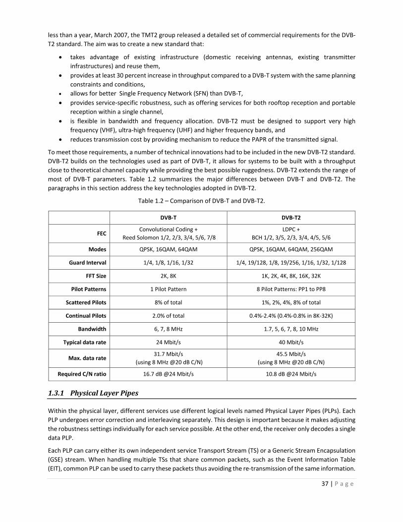
37 | P a g e
less than a year, March 2007, the TMT2 group released a detailed set of commercial requirements for the DVB‐
T2 standard.The aim was to create a new standard that:
takes advantage of existing infrastructure (domestic receiving antennas, existing transmitter
infrastructures) and reuse them,
provides at least 30 percent increase in throughput compared to a DVB‐T system with the same planning
constraints and conditions,
allows for better Single Frequency Network (SFN) than DVB‐T,
provides service‐specific robustness, such as offering services for both rooftop reception and portable
reception within a single channel,
is flexible in bandwidth and frequency allocation. DVB‐T2 must be designed to support very high
frequency (VHF), ultra‐high frequency (UHF) and higher frequency bands, and
reduces transmission cost by providing mechanism to reduce the PAPR of the transmitted signal.
To meet those requirements, a number of technical innovations had to be included in the new DVB‐T2 standard.
DVB‐T2 builds on the technologies used as part of DVB‐T, it allows for systems to be built with a throughput
close to theoretical channel capacity while providing the best possible ruggedness. DVB‐T2 extends the range of
most of DVB‐T parameters. Table 1.2 summarizes the major differences between DVB‐T and DVB‐T2. The
paragraphs in this section address the key technologies adopted in DVB‐T2.
Table 1.2 – Comparison of DVB‐T and DVB‐T2.
DVB‐T DVB‐T2
FEC Convolutional Coding +
Reed Solomon 1/2, 2/3, 3/4, 5/6, 7/8
LDPC +
BCH 1/2, 3/5, 2/3, 3/4, 4/5, 5/6
Modes QPSK, 16QAM, 64QAM QPSK, 16QAM, 64QAM, 256QAM
Guard Interval 1/4, 1/8, 1/16, 1/32 1/4, 19/128, 1/8, 19/256, 1/16, 1/32, 1/128
FFT Size 2K, 8K 1K, 2K, 4K, 8K, 16K, 32K
Pilot Patterns 1 Pilot Pattern 8 Pilot Patterns: PP1 to PP8
Scattered Pilots 8% of total 1%, 2%, 4%, 8% of total
Continual Pilots 2.0% of total 0.4%‐2.4% (0.4%‐0.8% in 8K‐32K)
Bandwidth 6, 7, 8 MHz 1.7, 5, 6, 7, 8, 10 MHz
Typical data rate 24 Mbit/s 40 Mbit/s
Max. data rate 31.7 Mbit/s
(using 8 MHz @20 dB C/N)
45.5 Mbit/s
(using 8 MHz @20 dB C/N)
Required C/N ratio 16.7 dB @24 Mbit/s 10.8 dB @24 Mbit/s
1.3.1 PhysicalLayerPipes
Within the physical layer, different services use different logical levels named Physical Layer Pipes (PLPs). Each
PLP undergoes error correction and interleaving separately. This design is important because it makes adjusting
the robustness settings individually for each service possible. At the other end, the receiver only decodes a single
data PLP.
Each PLP can carry either its own independent service Transport Stream (TS) or a Generic Stream Encapsulation
(GSE) stream. When handling multiple TSs that share common packets, such as the Event Information Table
(EIT), common PLP can be used to carry these packets thus avoiding the re‐transmission of the same information.

38 | P a g e
At the receiver, the content of the common PLP is merged with the user specific PLP to reconstruct the TS. Cyclic
Redundancy Check (CRC) bits are then inserted by the mode and stream adaption block, which also compresses
null MPEG2 packets. DVB‐T2 uses the same Forward Error Correction (FEC) mechanisms as DVB‐S2. In order to
provide immunity against impulse interference, time interleavers of at least 70ms are used.
1.3.2 IFFTSize
DVB‐T2 uses OFDM for modulation. The OFDM symbol time for aDVB‐T2 can be increased by a factor of two (16K) and four (32K) compared to DVB‐T’s longest symbol (8K).
Figure 1.8 – Comparison of OFDM symbol length of DVB‐T and DVB‐T2.
For a given guard interval size, DVB‐T2 has a higher capacity than DVB‐T because it reduces the overhead due to
the GI and hence improves bandwidth efficiency (i.e. for the maximum guard interval (1/4) and largest IFFT size
(8K) in DVB‐T, the GI overhead in DVB‐T is 25%. In DVB‐T2, the same GI length can be achieved with a 32K IFFT
and GI of 1/16, see Figure 1.8. The overhead for the same GI length drops to around 6%). For the same GI
fraction, DVB‐T2 can have a larger SFN coverage.
1.3.3 FrameStructure
The data cells at the output of the interleavers are mapped into OFDM symbols. Signaling information is then
added to these symbols in order to construct the DVB‐T2 frames. The DVB‐T2 frame structure is shown in Figure
1.9.
Figure 1.9 – Structure of DVB‐T2 frames.
Superframes are at the top level, they have a maximum duration of 64 seconds. Each superframe is divided into
DVB‐T2 frames which are further divided into OFDM symbols.
Each frame carries a configurable number of OFDM data symbols and starts with a preamble consisting of one
reference symbol called P1 followed by at least one reference symbol called P2. The number of P2 symbols,
depends on the IFFT size used (Table 1.3). The duration of frame varies between 100 and 250 milliseconds. The
DVB‐T2 frame structure can achieve a high time diversity, by spreading the data evenly across a whole frame,
or by allowing for power saving techniques to be used at the receiver side by concentrating data into bursts.

39 | P a g e
Table 1.3 – Number of P2 symbols for different FFT modes.
FFT size
1K 16
2K 8
4K 4
8K 2
16K 1
32K 1
The P1 symbol is designed to allow the receiver to derive a time reference for each frame. The P1 symbol carries
only seven bits of information coded on 384 out of the 1024 subcarriers using a Differential BPSK (DBPSK). These
seven bits carry limited signaling information such as the size of the IFFT and use of FEF frames. The P1 symbol
is also used by the receiver to detect the presence of DVB‐T2 signals. Its structure and design allow for both a
fast scan of the broadcast frequencies and improved robustness in the presence of challenging channel
conditions such as a zero dB echoes with opposite phases.
The P2 symbols mainly carries the dynamic L1 signaling information that contains the position, in time and
frequency, of the cells for each PLP. The L1 signaling can be large, because each PLP has different transmission
parameters. L1 signaling is very important because the information it carries is used by the receiver in order to
extract the user selected data PLP and the common PLP. This is why it has been given practical design care (it
undergoes various error correction, detection and repetition), in particular to assure robustness against impulse
noise that can affect DVB‐T2 systems with static reception. The P2 has another role that of imitating the channel
estimation process.
Future Extension Frames (FEFs) can be optionally included into superframes. FEF are designed to allow for future
services to be integrated. When FEF are used the maximum duration of 64s for a superframe may be exceeded.
In July 2011, FEF have been used for the first time with T2‐Lite [38] which is an additional transmission profile
type design to reduce implementation costs and to support mobile and portable TV. T2‐Lite incorporated only
the elements relevant to mobile and portable reception with a restricted data rate of 4 Mbps. Even though T2‐
Lite uses different FFT sizes and GI length than the base DVB‐T2 (T2‐base), the use of FEF enables T2‐Lite and
T2‐base to be transmitted in the same RF channel.
1.3.4 ForwardErrorCorrection
DVB‐T uses convolutional codes and Reed‐Solomon for Forward Error Correction (FEC). In order to achieve up
to 30 percent more capacity, for the same robustness, DVB‐T2 uses a concatenated LDPC [39] [40] (Low‐Density
Parity Check) and BCH (Bose‐Chaudhuri‐Hocquenghem) [41] code. This is the same technique used in DVB‐S2
and DVB‐C2 standards.
Each logical data stream input is sliced in data fields called baseband frames (BBFRAMES). Check bits of the BCH
code and of the LDPC code are added to form the FECFRAME. DVB‐T2 specifies two FECFRAME length values,
long (64,800 bits) and short (16,200 bits). Long frames require complex receivers and cause latency, but reduce
overall overhead compared to short frames. DVB‐T2 specifies 6 different code rates that can be used to make
trade‐offs between robustness and capacity.
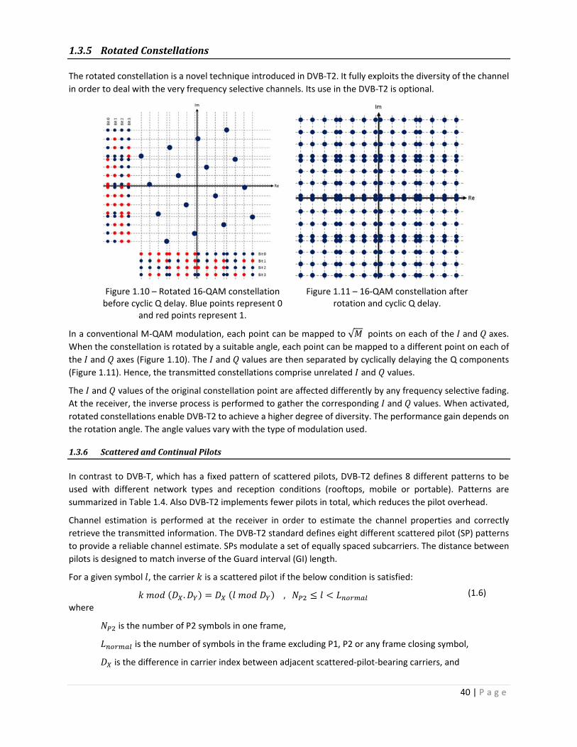
40 | P a g e
1.3.5 RotatedConstellations
The rotated constellation is a novel technique introduced in DVB‐T2. It fully exploits the diversity of the channel
in order to deal with the very frequency selective channels. Its use in the DVB‐T2 is optional.
Figure 1.10 – Rotated 16‐QAM constellation before cyclic Q delay. Blue points represent 0
and red points represent 1.
Figure 1.11 – 16‐QAM constellation after rotation and cyclic Q delay.
In a conventional M‐QAM modulation, each point can be mapped to √ points on each of the and axes. When the constellation is rotated by a suitable angle, each point can be mapped to a different point on each of
the and axes (Figure 1.10). The and values are then separated by cyclically delaying the Q components
(Figure 1.11). Hence, the transmitted constellations comprise unrelated and values.
The and values of the original constellation point are affected differently by any frequency selective fading. At the receiver, the inverse process is performed to gather the corresponding and values. When activated,
rotated constellations enable DVB‐T2 to achieve a higher degree of diversity. The performance gain depends on
the rotation angle. The angle values vary with the type of modulation used.
1.3.6 ScatteredandContinualPilots
In contrast to DVB‐T, which has a fixed pattern of scattered pilots, DVB‐T2 defines 8 different patterns to be
used with different network types and reception conditions (rooftops, mobile or portable). Patterns are
summarized in Table 1.4. Also DVB‐T2 implements fewer pilots in total, which reduces the pilot overhead.
Channel estimation is performed at the receiver in order to estimate the channel properties and correctly
retrieve the transmitted information. The DVB‐T2 standard defines eight different scattered pilot (SP) patterns
to provide a reliable channel estimate. SPs modulate a set of equally spaced subcarriers. The distance between
pilots is designed to match inverse of the Guard interval (GI) length.
For a given symbol , the carrier is a scattered pilot if the below condition is satisfied:
. , (1.6)
where
is the number of P2 symbols in one frame,
is the number of symbols in the frame excluding P1, P2 or any frame closing symbol,
is the difference in carrier index between adjacent scattered‐pilot‐bearing carriers, and

41 | P a g e
is the number of symbols forming one scattered pilot sequence.
The equality in (1.6) is important in this study because it shows that scattered pilot positions vary from one
OFDM symbol to another.
Table 1.4 – Scattered pilots parameters.
Scattered Pilot Pattern
PP1 3 4
PP2 6 2
PP3 6 4
PP4 12 2
PP5 12 4
PP6 24 2
PP7 24 4
PP8 6 16
Another set of pilots called Continual Pilots (CPs) are used for common phase error correction and frequency
synchronization. CPs are matched to the IFFT size. Channel estimation can be efficiently tuned for any given
channel by using the extended range of CPs and SPs.
Other types of pilots exist such as Edge pilots, P2 pilots and Frame‐Closing Pilots. The following list summarizes
the uses for pilots in DVB‐T2
the scattered, P2 and Frame‐Closing pilots can be used for channel estimation and equalization,
the continual, P2 and Frame‐Closing pilots can be used for Common‐Phase‐Error correction,
all the pilots can potentially be used for Synchronization,
continual, P2 and Frame‐Closing pilots are also used as a form of 'padding', and
edge pilots are used for frequency interpolation up to the edge of the spectrum.
Table 1.5 shows the compatibility between symbol types and pilot types.
Table 1.5 ‐ Presence of pilots in each type of symbol.
Symbol Pilot Type
Scattered Continual Edge P2 Frame‐Closing
P1
P2 X
Normal X X X
Frame‐closing X X
1.3.7 MultipleInputSingleOutput
In order to support Single‐Frequency Networks (SFN), the DVB‐T standard allows for multiple transmitters to
transmit, simultaneously, the same signal on the same frequency. Destructive interference occurs at the receiver
when similar‐strength signals are received from two transmitters. This phenomenon causes deep nulls to appear
in the channel frequency and yields poor performance.
DVB‐T2 uses a modified form of Alamouti [42] encoding that takes advantage of the presence of multiple
transmitters. The Alamouti scheme is a Multiple Input Single Output (MISO) system with two transmitters (TX1
and TX2). To avoid deep channel nulls, for each constellation point pair 0, 1 transmitted by TX1, TX2

42 | P a g e
transmits a slightly modified pair. The receiver performs an optimum combination of the two signals. The
Alamouti scheme improves the SFN since the resulting signal‐to‐noise ratio is a though the powers of the two
signals had been combined. The Alamouti mechanism requires slightly higher complexity receivers (extra
multipliers, duplicate channel estimation, double the density of scattered pilots), and its use is optional.
1.3.8 MarketDeployment
The market emerged in 1998 with the first generation DTT standard (DVB‐T) and started growing as of 2008 with
the second generation standard (DVB‐T2) which was successful on the international level. There is nearly 1
billion DVB receivers deployed all around the world. Figure 1.12 shows the adoption of various DTTB standards
in the world (The blue colors shows countries that have adopted or deployed DVB‐T and DVB‐T2 on December
2014).
Figure 1.12 ‐ DTT systems [43].
DVB‐T2 was first deployed in the UK in 2010. Multiple countries (Sweden, Italy and Finland) followed shortly. At
the time being almost every European country is studying plan to switch from DVB‐T to DVB‐T2. Countries in
Africa and Asia also adopted the standard; in total more than 40 countries have adopted the standard and 28
deployed it.
1.4 Conclusion
This first chapter introduced the principle behind the OFDM technique, which has been used in multiple wired
and wireless telecommunication standards, and showed its efficiency in dealing with ISI caused by multipath in
radio transmission systems. It also described the high power fluctuations which is one of the disadvantages of
OFDM and MC systems in general. A brief description of DTTB standards worldwide was also given followed by
a detailed description of the key technologies used in the DVB‐T2.

43 | P a g e
High Power Amplifiers
and PAPR Reduction Techniques
OFDM systems in general, and DVB‐T2 in particular, suffer from high Peak to Average Power Ratio (PAPR). High
PAPR has a direct impact on High Power Amplifier (HPA) performance. In this chapter, Section 1.1 is dedicated
to explain the nonlinearities of HPA and their impact on system performance. Section 2.2 explains how reducing
the OFDM signal fluctuations, hence reducing the PAPR, can enhance HPA performance. The two PAPR reduction
techniques adopted in DVB‐T2 standard, i.e. the Tone Reservation (TR) and Active Constellation Extension (ACE),
in Section 2.3, whereas other PAPR reduction techniques proposed in the literature but not adopted by DVB‐T2
are presented in Section 2.3.
2.1 HighPowerAmplifiers
In order to demodulate the received signal and maintain an acceptable BER, the receiver requires a minimum
Signal to Noise Ratio (SNR). Multiple sources of noise can exist at the receiver. Furthermore radio frequency
signals are attenuated by a factor proportional to the square of the distance traveled between the transmitter
and the receiver. The role of the HPA is to boost the transmitted signal power to compensate for the signal
attenuation and to ensure the received signal power is high enough compared to the receiver noise [44].
Ideally, the amplified signal keeps the same form as the original signal. However amplifier circuits are built from
active components with nonlinear characteristics. Nonlinearities encountered in multi‐carrier communication
transceivers cause the transmitted signal to be distorted. This causes ICI and Bit Error Rate (BER) degradation
that affect the performance. The main nonlinearity sources are the quantization errors due to digital to analog
conversion and the nonlinearity of the HPA. The nonlinearity of the HPA has the most impact due to the power
fluctuation of multi‐carrier signals.To better understand this phenomenon, this section takes a closer look on
the nonlinear characteristics of HPAs.

44 | P a g e
2.1.1 PowerBalanceandGain
A power amplifier takes an input signal of power and generates an output signal of power . To operate,
the amplifier consumes battery power . The amplification process is not ideal and a certain amount of power
is dissipated.
The relationship between these power values (see Figure 2.1) is given by:
Figure 2.1 – HPA power relationship
The gain of an amplifier is defined by:
2.1.2 Classes
There are two main types of Power Amplifiers: Travelling Wave Tube Amplifier (TWTA) and Solid State Power
Amplifier (SSPA). TWTAs are widely used in satellite communication systems and deliver high power levels.
SSPAs are mainly used in terrestrial radio communications such as DVB‐T2.
Amplifiers can be divided into two main categories:
Linear amplifiers (class A, B and AB): they are mainly used with signals whose envelops are not constant,
such as the OFDM signals.
Nonlinear amplifiers (class C, D, E, F, H and S): they are used in systems with constant signal envelop
thus not affected by nonlinearities.
In this thesis, only linear SSPA amplifiers are considered.
2.1.3 TransferCharacteristics
The HPA can be modeled as a memory‐less device. Let represent the input of the amplifier and its
output.
.
.
where and represent the amplitude over time, and and Φ represent the phase.
The transfer characteristics of a power amplifier describe the relationship between the input and the output
signal of the amplifier:
The Amplitude to Amplitude (AM/AM) relates the input amplitude to the output amplitude.

45 | P a g e
The Amplitude to Phase (AM/PM) relates the input amplitude to the output phase variation.
Φ ,
2.1.3.1 Amplitude to Amplitude
Figure 2.2 – AM/AM characteristics of an HPA.
Figure 2.3 – HPA Gain.
As depicted in Figure 1.2Figure 2.2 and Figure 2.3 the characteristics of an HPA can be divided into three zones:
Zone 1 – Linear Zone: In this zone, the output amplitudes are proportional to the input amplitude. The
ratio of the output power to the input power is constant in this zone and is referred to as the power
amplifier gain. In this zone the power range is low and distortion is almost inexistent.
Zone 2 – Compression Zone: The output amplitude is no longer proportional to the input amplitude in
this zone. The amplifier gain is not constant and starts decreasing. As input amplitude increases the
output becomes more and more distorted.
Zone 3 – Saturation Zone: This is the zone were nonlinearities become most evident. Increasing the
input amplitude has no effect on the output whose amplitude remains almost constant. The output
power is referred to as , . The gain decreases sharply in this zone.
Two points are also important to consider:
Compression point: The compression point is the point where the gap between the ideal linear gain
curve and the actual (practical gain curve) is equal to 1 decibel (dB). The coordinates of the points are
noted , and , .
Operating point: The operation point is established by a process known as Biasing. Biasing sets the
correct operating point of the transistor amplifier and can be looked at as adding a DC component to
the input signal.
2.1.3.2 Amplitude to Phase
The AM/PM characteristics change with the techniques used to fabricate the HPA and depend on the operating
conditions [45]. For SSPA amplifiers, the phase distortion is small enough to be neglected:
Φ
2.1.4 Efficiency
The power efficiency of a power amplifier is given by:
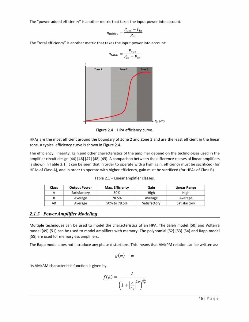
46 | P a g e
The “power‐added efficiency” is another metric that takes the input power into account:
The “total efficiency” is another metric that takes the input power into account:
Figure 2.4 – HPA efficiency curve.
HPAs are the most efficient around the boundary of Zone 2 and Zone 3 and are the least efficient in the linear
zone. A typical efficiency curve is shown in Figure 2.4.
The efficiency, linearity, gain and other characteristics of the amplifier depend on the technologies used in the
amplifier circuit design [44] [46] [47] [48] [49]. A comparison between the difference classes of linear amplifiers
is shown in Table 2.1. It can be seen that in order to operate with a high gain, efficiency must be sacrificed (for
HPAs of Class A), and in order to operate with higher efficiency, gain must be sacrificed (for HPAs of Class B).
Table 2.1 – Linear amplifier classes.
Class Output Power Max. Efficiency Gain Linear Range
A Satisfactory 50% High High
B Average 78.5% Average Average
AB Average 50% to 78.5% Satisfactory Satisfactory
2.1.5 PowerAmplifierModeling
Multiple techniques can be used to model the characteristics of an HPA. The Saleh model [50] and Volterra
model [49] [51] can be used to model amplifiers with memory. The polynomial [52] [53] [54] and Rapp model
[55] are used for memoryless amplifiers.
The Rapp model does not introduce any phase distortions. This means that AM/PM relation can be written as:
Its AM/AM characteristic function is given by
1

47 | P a g e
where is the limiting output amplitude, and is the so‐called knee factor representing the linearity of the
amplifier.
Different curves for different values of are shown in Figure 2.5. When is equal to 100, the amplifier is quasi
linear up to an input amplitude equal to , when decreases the nonlinear distortion starts increasing.
Figure 2.5 – AM/AM of Rapp model for different values of and 1.
The RAPP model is chosen to model the HPA in this study. Its constant AM/PM characteristics makes it suitable
to model SSPAs phase distortion. And its AM/AM can be easily tuned to simulate various non linearity levels.
2.1.6 ModulationErrorRateandErrorVectorMagnitude
Modulation Error Rate (MER) is defined in the European Telecommunications Standards Institute (ETSI)
Technical Report 101 290 [56], which describes the measurement guidelines for DVB systems. MER gives an
indication of the ability of the receiver to correctly decode the signal. The MER computation gives a figure of
merit for system performance by comparing the actual location of a received sample to its ideal location ,
see Figure 2.6. The MER value decreases when degradation occurs.
,∑
∑ | |
To assess the performance of the HPA, is measured at the input of the amplifier and is measured at the
output of the amplifier.
Figure 2.6 – Error vector.
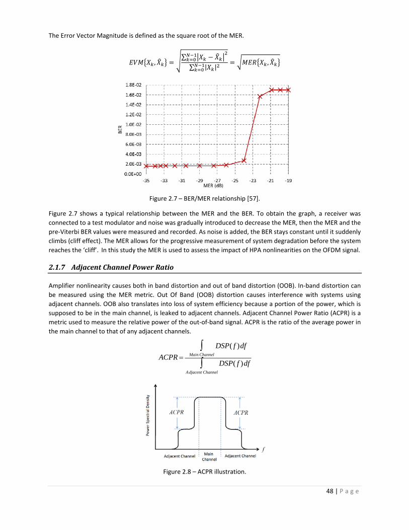
48 | P a g e
The Error Vector Magnitude is defined as the square root of the MER.
,∑
∑ | |,
Figure 2.7 – BER/MER relationship [57].
Figure 2.7 shows a typical relationship between the MER and the BER. To obtain the graph, a receiver was
connected to a test modulator and noise was gradually introduced to decrease the MER, then the MER and the
pre‐Viterbi BER values were measured and recorded. As noise is added, the BER stays constant until it suddenly
climbs (cliff effect). The MER allows for the progressive measurement of system degradation before the system
reaches the ‘cliff’. In this study the MER is used to assess the impact of HPA nonlinearities on the OFDM signal.
2.1.7 AdjacentChannelPowerRatio
Amplifier nonlinearity causes both in band distortion and out of band distortion (OOB). In‐band distortion can
be measured using the MER metric. Out Of Band (OOB) distortion causes interference with systems using
adjacent channels. OOB also translates into loss of system efficiency because a portion of the power, which is
supposed to be in the main channel, is leaked to adjacent channels. Adjacent Channel Power Ratio (ACPR) is a
metric used to measure the relative power of the out‐of‐band signal. ACPR is the ratio of the average power in
the main channel to that of any adjacent channels.
ACPR DSP( f )df
Main Channel
DSP( f )df
Adjacent Channel
Figure 2.8 – ACPR illustration.

49 | P a g e
2.2 ThePAPRProblem
2.2.1 InputBackOff
To avoid nonlinearities, operating the amplifier in the saturation zone must be avoided. Normally the operating
point is backed‐off to the linear zone such as the peaks of the input signal never enter the nonlinear zones. The
Input Back Off (IBO) is defined as the gap between the 1 dB compression point and the operating point:
:
or in decibel,
:
With enough back‐off the operating point can be moved to the linear region thus eliminating any possible
distortion [58]. This solution has two main disadvantages:
In the linear region, the power efficiency of the amplifier is very low. A big portion of the energy is
dissipated and lost. It is not economical to operate in this zone.
In this region, the output power is relatively low. This makes the transmitted signal more sensitive to
channel noise and results in a lower SNR at the receiver thus causing poor system performance.
2.2.2 IBOandMER
In the simulations performed in thesis, the IBO and MER are used together to assess the performance of the
HPA: for a given HPA configuration, the IBO is varied; for each IBO value the signal is amplified and ,
is computed for signal before amplification and after amplification .
As in the DVB‐T2 standard, the target MER is set to ‐40 dB. The lower the IBO required, the better the
configuration. This is because with a lower IBO the HPA operates closer to the boundary between zone 2 and
zone 3 (see paragraph 2.1.4) hence its energy efficiency is higher.
2.2.3 LinearizationTechniques
In the right most region of Zone 2 (near the border with Zone 3, Figure 2.3 and Figure 2.4) both the efficiency
and output power are relatively high. However this region is also characterized by a high level of distortion. To
operate in this region, multiple amplifier linearization techniques are possible such as:
Linear Amplification using Nonlinear Components (LINC) [59],
Envelope Elimination and Restoration (EER) [60],
Envelope Tracking (ET) [61],
Feedback technique [62] [63],
Feed‐forward technique [64], and
Predistortion technique [65].
Predistortion is implemented with the actual amplifiers used for testing and measurement in paragraph 4.3. The
principle is illustrated in Figure 2.9. The predistortion module has transfer characteristic functions equal to the
inverse of the amplifier's characteristic. When the HPA is combined with the corresponding predistortion
module, the overall transfer function becomes more linear.

50 | P a g e
Figure 2.9 – Predistortion illustration.
Predistortion techniques are not covered in this thesis, however their impact on PAPR reduction is discussed in
paragraph 3.1.9.
2.2.4 LimitingSignalFluctuations
Another way to reduce the impact of distortion in the high efficiency zone, is to limit the amount of fluctuation
of the input signal. This principle is illustrated in Figure 2.10 and Figure 2.11. Figure 2.10 shows how a signal with
high power fluctuations can experience a higher amount of distortion. A signal with lower power fluctuations,
as shown in Figure 2.11, experiences a more linear amplifier yet high power gain. Moreover, a signal with low
fluctuations allows the HPA to operate in a higher efficiency region (closer to the border between zone 2 and
zone 3).
Figure 2.10 – Input signal with high power fluctuations.

51 | P a g e
Figure 2.11 – Input signal with low power fluctuations.
2.2.5 PAPRDefinition
The Peak to Average Power Ratio is a metric used to assess the amount of signal fluctuations.
Let . be a complex baseband signal. The PAPR of the continuous signal is given by:
max| |
lim→
| |
The Crest Factor (CF) is defined as the square root of PAPR [66]:
The PAPR for a discrete time symbol, , is defined as:
max| |
| |
where {} is the expectation operator.
For an M‐ary QAM modulation, with modulation states, the maximum PAPR is given by [67]:
, 3√ 1
√ 1
The probability of that maximum occurring is equal to [68].

52 | P a g e
2.2.6 ComplementaryCumulativeDistributionFunctionsofthePAPRofOFDMSignals
For an OFDM system with 1024 subcarriers with QPSK modulation ( 4 , the highest possible PAPR value
occurs when all subcarriers carry the same symbol. The probability of reaching this maximum PAPR value is
equal to2 .
For a DVB‐T2 symbol size of 1K with a symbol duration of 0.112 μs, the maximum PAPR occurs once every
3.55 2 years. In practical scenarios this bound is never reached. Hence there is a need for statistical
methods to take better advantage of the PAPR metric.
The Complimentary Cumulative Distribution Function (CCDF) is defined as the probability that the PAPR of
transmitted OFDM symbols exceeds a threshold value .
For large values of , the CCDF is given by [69]:
1
However, it is the analog version of that is actually amplified and transmitted. Oversampling can be applied to
in order to render the CCDF measurements closer to those of the analog version. However, in this case the
samples are not mutually uncorrelated. The PAPR CCDF for subcarriers ( > 64) and oversampling can be
approximated by the distribution of subcarriers without oversampling, with equal to 2.8 [69]:
1 .
Another approximation of the CCDF of the analog OFDM is given by [70]:
3√
2.3 PAPRReductionTechniques
This section is dedicated to the multiple PAPR reduction techniques proposed in the literature. It also details the
two PAPR reduction techniques adopted by DVB‐T2: the Active Constellation Extension (ACE) and Tone
Reservation (TR), the latter being extensively studied in the remainder of this work.
2.3.1 AmplitudeClippingandFiltering
Clipping is the simplest PAPR reduction technique [71]. The signal amplitude is clipped when it exceeds a
predefined threshold :
, | | ∅ , | |
The clipping introduces distortion that can be viewed as a source of noise that falls both out‐of‐band and in‐
band. The in‐band distortion is reflected in a degradation of error performance. The out‐of‐band reduces the
spectral efficiency, although an additional filtering step is able to limit such an effect.
It is to be noted that in some cases the filtering can cause peak regrowth to values exceeding the threshold used
for clipping. To mitigate this effect, clipping and filtering process can be repeated until reaching the desired
amplitude [72] at the cost of added computational complexity.
2.3.2 Coding
Coding as a mean to reduce the PAPR was introduced in [73]. The idea is to select among the available code
words those that minimize the PAPR and use them for transmission.
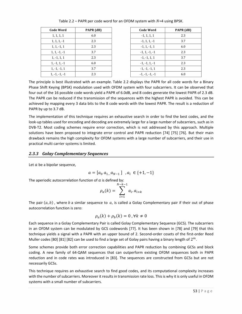
53 | P a g e
Table 2.2 – PAPR per code word for an OFDM system with =4 using BPSK.
CodeWord PAPR(dB) CodeWord PAPR(dB)
1,1,1,1 6.0 ‐1,1,1,1 2.3
1,1,1,‐1 2.3 ‐1,1,1,‐1 3.7
1,1,‐1,1 2.3 ‐1,1,‐1,1 6.0
1,1,‐1,‐1 3.7 ‐1,1,‐1,‐1 2.3
1,‐1,1,1 2.3 ‐1,‐1,1,1 3.7
1,‐1,1,‐1 6.0 ‐1,‐1,1,‐1 2.3
1,‐1,‐1,1 3.7 ‐1,‐1,‐1,1 2.3
1,‐1,‐1,‐1 2.3 ‐1,‐1,‐1,‐1 6.0
The principle is best illustrated with an example.Table 2.2 displays the PAPR for all code words for a Binary
Phase Shift Keying (BPSK) modulation used with OFDM system with four subcarriers. It can be observed that
four out of the 16 possible code words yield a PAPR of 6.0dB, and 8 codes generate the lowest PAPR of 2.3 dB.
The PAPR can be reduced if the transmission of the sequences with the highest PAPR is avoided. This can be
achieved by mapping every 3 data bits to the 8 code words with the lowest PAPR. The result is a reduction of
PAPR by up to 3.7 dB.
The implementation of this technique requires an exhaustive search in order to find the best codes, and the
look‐up tables used for encoding and decoding are extremely large for a large number of subcarriers, such as in
DVB‐T2. Most coding schemes require error correction, which is not addressed by this approach. Multiple
solutions have been proposed to integrate error control and PAPR reduction [74] [75] [76]. But their main
drawback remains the high complexity for OFDM systems with a large number of subcarriers, and their use in
practical multi carrier systems is limited.
2.3.3 GolayComplementarySequences
Let be a bipolar sequence,
… , ∈ 1, 1
The aperiodic autocorrelation function of is defined by:
.
The pair , , where a similar sequence to , is called a Golay Complementary pair if their out of phase
autocorrelation function is zero:
0, ∀ 0
Each sequence in a Golay Complementary Pair is called Golay Complementary Sequence (GCS). The subcarriers
in an OFDM system can be modulated by GCS codewords [77]. It has been shown in [78] and [79] that this
technique yields a signal with a PAPR with an upper bound of 2. Second‐order cosets of the first‐order Reed
Muller codes [80] [81] [82] can be used to find a large set of Golay pairs having a binary length of 2 .
Some schemes provide both error correction capabilities and PAPR reduction by combining GCSs and block
coding. A new family of 64‐QAM sequences that can outperform existing OFDM sequences both in PAPR
reduction and in code rates was introduced in [83]. The sequences are constructed from GCSs but are not
necessarily GCSs.
This technique requires an exhaustive search to find good codes, and its computational complexity increases
with the number of subcarriers. Moreover it results in transmission rate loss. This is why it is only useful in OFDM
systems with a small number of subcarriers.

54 | P a g e
2.3.4 PartialTransmitSequence
The idea of Partial Transmit Sequence (PTS) is based on the partitioning of a data block of size N, into M disjoint
sub‐blocks of size [84]:
An example of sub‐block partitioning is shown in Figure 2.12.
Figure 2.12 ‐ Sub‐block partitioning in PTS.
The time domain representations of are called the partial transmit sequences and are denoted . Before
being re‐combined, each sequence is multiplied by a complex phase factor .
.
An exhaustive search is needed to find the phase factors that minimize the PAPR of the combined sequences. In
practice, the phase factors are limited to a set with a finite number of elements. The PAPR reduction increases
with the number of sub‐blocks used, so does the search complexity, which increases exponentially.
Side information about the chosen phase factors needs to be sent to the receiver. The sub‐blocks can be
generated using different types of partitioning: adjacent, interleaved, and pseudo‐random partitioning [85]. The
PTS technique can be adapted to any modulation scheme and any number of subcarriers.
Figure 2.13 – Block Diagram of the PTS technique.

55 | P a g e
2.3.5 SelectedMappingTechnique
The Selected Mapping (SLM) technique uses the original data block, to generate different candidates blocks, all
representing the same information, and selects the one with lowest PAPR for transmission [86] [87].Figure 2.14
shows a block diagram of the SLM technique.
Figure 2.14 – Block Diagram of the SLM technique.
Each candidate block is obtained by multiplying the original data block by a different phase sequence
of length N. An IDFT is then used to generate the time domain version of each block. The candidate with the
lowest PAPR is then selected for transmission.
The receiver needs to know which block has been selected for each OFDM symbol. In order to correctly
demodulate the signal, the receiver must perform the reverse operation to recover the original data block. SLM
requires side information about the selected phase sequence to be sent to the receiver.
Factors such as the number of candidate blocks used and the design of the phase sequences impact the amount
of PAPR reduction.
2.3.6 InterleavingTechnique
Similar to SLM, the interleaving technique generates multiple candidates carrying the same information and
selects the one with the lowest PAPR for transmission. Instead of using phase sequences to generate the
different candidates, the interleaving technique uses multiple interleavers [88] [89] [90]. Each interleaver
reorders the N symbols of the original data block in order to generate a candidate. The transmitter and the
receiver store all possible permutations in memory, this way only the index of the interleaver used needs to be
sent as side information.
2.3.7 ToneInjection
A data stream is divided into code words, each code word is then mapped to specific constellation point. The
PAPR corresponding to the transmission of a given constellation point can be modified by changing its real
and/or imaginary parts [91].
If the changes to can be estimated at the receiver, there is no need to exchange any side information. A simple
approach is to generate the modified version of as follows:
. . .
where is a positive real number known at the receiver and and are any integer value. Figure 2.15 shows
some possible candidates for a given constellation point, the corresponding and values are displayed in
Table 2.3.

56 | P a g e
Table 2.3 – New constellation point candidates.
1 1
0 1
‐1 1
‐1 0
‐1 ‐1
0 ‐1
1 ‐1
1 0
The choice of is very important. Values that cause the generated points to overlap with existing constellation
points need to be avoided along with values that cause the minimum distance between points to decrease. The
value of must be big enough to make sure that the Symbol Error Rate (SER) of the system does not change.
The new constellation points create an extra degree of freedom that can be used to reduce the PAPR of the
transmitted signal. Multiple algorithms for the choice of and has been proposed in [91].
Figure 2.15 – Tone Injection with 16 QAM constellation.
2.3.8 ToneReservation
2.3.8.1 Concept
The idea behind the Tone Reservation concept was introduced by Tellado in 1997 [92]. In 2000 Tellado published
a book [93] following his thesis detailing his findings. TR relies on reserving M subcarriers (referred to as reserved
tones), out of the total of N subcarriers, for PAPR reduction purposes.
Let be the set of reserved pilot positions.
, … , (2.1)
Let represent the useful data signal and let represent the reserved tones. The transmitted signal is given
by:
∈ , 0 (2.2)
where
0if ∉
0 ∈
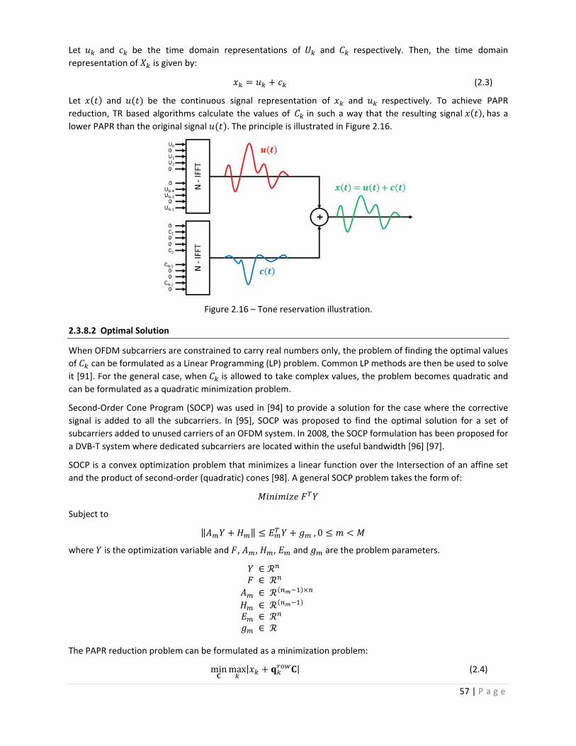
57 | P a g e
Let and be the time domain representations of and respectively. Then, the time domain
representation of is given by:
(2.3)
Let and be the continuous signal representation of and respectively. To achieve PAPR
reduction, TR based algorithms calculate the values of in such a way that the resulting signal , has a lower PAPR than the original signal . The principle is illustrated in Figure 2.16.
Figure 2.16 – Tone reservation illustration.
2.3.8.2 Optimal Solution
When OFDM subcarriers are constrained to carry real numbers only, the problem of finding the optimal values
of can be formulated as a Linear Programming (LP) problem. Common LP methods are then be used to solve
it [91]. For the general case, when is allowed to take complex values, the problem becomes quadratic and
can be formulated as a quadratic minimization problem.
Second‐Order Cone Program (SOCP) was used in [94] to provide a solution for the case where the corrective
signal is added to all the subcarriers. In [95], SOCP was proposed to find the optimal solution for a set of
subcarriers added to unused carriers of an OFDM system. In 2008, the SOCP formulation has been proposed for
a DVB‐T system where dedicated subcarriers are located within the useful bandwidth [96] [97].
SOCP is a convex optimization problem that minimizes a linear function over the Intersection of an affine set
and the product of second‐order (quadratic) cones [98]. A general SOCP problem takes the form of:
Subject to
‖ ‖ , 0
where is the optimization variable and , , , and are the problem parameters.
∈ ∈ ∈ ∈ ∈ ∈
The PAPR reduction problem can be formulated as a minimization problem:
minmax| | (2.4)

58 | P a g e
where is the row of the IDFT matrix of size .
Equation (2.4) is equivalent to:
| | , 0, … ,
and can be reformulated, as described in [99], into an SOCP problem as follows:
0 … 1 ∈
0 … 0 1 ∈ 0 … 0 1 ∈
, , … , , 0 ∈
where
,
cos 2π.
sin 2π. and ,
sin 2π.
cos 2π.
The solution of the SOCP provides the optimal values to assign to the pilots tones in order to obtain the lowest
PAPR signal. However, the SOCP implementation is computationally complex.
Multiple research studies suggested approximations in order to solve the problem using a geometric approach
[100], Gradient methods [101] [102] [103] [104] and Active Set methods [105] [106] [107]. The performance and
the convergence vary from one method to another. However, all these methods share one criteria: they are all
too complex to implement in real‐time.
2.3.8.3 TR in DVB‐T2
An iterative TR algorithm has been adopted in DVB‐T2. The algorithm uses an impulse‐like kernel obtained by
assigning a value of one to all reserved tones and zero for the remaining subcarriers [93]. In time domain, the
kernel is characterized by a maximum, 0 , at position =0 (see Figure 2.18).
Figure 2.17 – Kernel shape for 32K mode.
At each iteration, the algorithm:
detects the highest peak, of amplitude , of the time domain signal,
circularly shifts a copy of the kernel in order for the kernel’s peak to coincide with that peak,
scales the kernel’s amplitude, and
adjusts its phase in such a way that its sum with the signal reduces the detected peak amplitude.
The same process is then repeated to detect and reduce another signal peak. The algorithm predefines an
amplitude threshold, Vclip, and exits when all signal peaks are below Vclip or when the maximum number of

59 | P a g e
iterations (called Iter) has been reached. The TR algorithm used in DVB‐T2, which is at the center of interest in
this manuscript, is discussed in more details in paragraph 3.1.
2.3.8.4 Recent Trends
Since then the interest in TR techniques has been growing, Figure 2.18 shows the number of publications per
year related to the search “tone reservation” in IEEExplore. Although the numbers are not representative of all
research relating to TR, they show the recent interest of the scientific community in the technique.
Figure 2.18 ‐ Number of publications, per year, relating to the search term “Tone Reservation” in IEEExplore.
Multiple researches focused on enhancing the performance of TR based algorithms. In [108], authors proposed
a scheme allowing for 25% of reserved TR band to carry additional noise, hence enhancing the SNR of data
carriers. To enhance spectral efficiency, Gold sequences are used in [109] to convey additional useful
information on the same sub‐carriers used for PAPR reductions. A method using the Moore‐Penrose generalized
inverse aiming to generate an ideal peak‐canceling signal is proposed in [110]. In [111], an approach based on
the Least Square Approximation (LSA) method and variance minimization techniques is used to generate the
time domain kernels. A very similar technique is also presented in [112] in the context of microwave
transmission (W‐Band). An adaptive Conjugate‐Gradient algorithm, based on the Polak‐Ribiere direction search,
is used in [113] to improve both the PAPR gain and the speed of convergence of PAPR reduction technique based
on TR. In [114], a new metric that allows for the measurement of nonlinearity impact on OFDM signals is used
to model the TR problem as an optimization problem, which can be sub‐optimally solved using a gradient based
adaptive scaling approach.
TR has also been proposed for OFDM variants and non‐OFDM systems that suffer from high PAPR. For example,
in [115] , the TR technique is adapted to the constraints of a digital up converter (DUC), which is a modern
software defined radio system that combines Third Generation Partnership Protocol (3GPP), Long Term
Evolution (LTE) and Universal Mobile Telecommunications System (UMTS). A suboptimal TR algorithm based on
Constant Amplitude Zero Auto‐Correlation (CAZAC) sequence and utilizing a fixed phase rotation method [116]
is used with a Multi‐Carrier Code Division Multiple Access (MC‐CDMA) system. TR has also been proposed to
reduce the PAPR of adaptive multicarrier modulations such Non‐Contiguous OFDM (NC‐OFDM) which is used in
Cognitive Radio (CR) at the physical layer level [117] where underlay transmission is used for the transmission
of the peak reducing carriers. Also in CR environments with NC‐OFDM, some tones available for the secondary
users can be allocated for the purpose of TR PAPR reduction of the primary user [118]. A TR based technique
has been proposed in [119] that takes advantages of attenuated frequency zones to insert the peak reducing
tones.
Methods to combine TR with other techniques have also been proposed. At the cost of higher complexity, better
PAPR reduction results may be obtained by combining the probabilistic selective mapping technique and tone
reservation such as in [120]. A Unitary‐Matrix Transformation UMT of the IFFT input vector is used in [121] to

60 | P a g e
allow the transmission chain to perform both pre and post IFFT PAPR reduction, the technique can be used with
the two post‐IFFT PAPR reduction algorithms (TR and ACE) specified in DVB‐T2 standard.
2.3.9 ActiveConstellationExpansion
Korngold and Jones in 1999 [122] introduced the Active Constellation Expansion (ACE) technique [123]. The
original version uses a Projection‐Onto‐Convex‐Sets (POCS) approach [124] to extend the outer points of a given
constellation to minimize the PAPR. The technique was too complex to be implemented in real‐time. Korngold
and Jones proposed, in 2003, an ACE implementation that was capable of faster PAPR reduction [125], [126].
This technique paved the way for ACE implementation in modern telecommunication standards.
2.3.9.1 Concept
To reduce the PAPR, ACE relies on modifying the signal constellation in data‐bearing channels without increasing
the BER. The best way to explain how the signal can be modified without affecting the BER is by the following
example: A QPSK constellation is shown in Figure 2.19. The constellation point (1,1) can be freely moved in the
shaded area without affecting the probability of error as the minimum distance (affecting the BER performance)
is unchanged.
Figure 2.19 ‐ ACE with a QPSK constellation.
Moving any point away from the constellation’s decision boundaries translates into either equal or lower error
rates, at the cost of an additional transmitted power. The principle can be applied to any constellation type such
as QAM and M‐PSK. For example, for QAM constellations, the outer points can be freely adjusted away from the
constellations (see Figure 2.20).
Figure 2.20 ‐ ACE with 64‐QAM.
61 | P a g e
All these modifications increase the transmitted signal power for the processed data block. The amount of added
power is in general proportional to the amplitude of the signal peaks. But in practice large signal peaks occur
rarely, thus these modifications have negligible impact on the total transmitted power.
Figure 2.20 shows that for a 64 QAM, out of the 64 points only 28 points can have their position modified for
PAPR reduction purposes that is only 43.75% compared to 100% for a QPSK constellation. Hence, when the
number of constellation points increases the percentage of points that can be manipulated decreases. This
results in ACE having poor performance for large constellations.
In DVB‐T2 the receiver performs LDPC decoding by using Log Likelihood Ratios (LLRs). ACE can potentially affect
the LDPC decoding in the receiver, since the LLR makes the assumption that additive noise is the only factor
causing constellation points to move off the QAM grid. When ACE is activated constellation measures which are
used to estimate interference and noise level (such as the average distance from the nearest constellation point)
can also be misleading.
ACE is not suitable for use in conjunction with rotated constellations. In DVB‐T2, ACE must indeed be disabled
when rotated constellations (paragraph 1.3.5) are used. The implementation of ACE, as described in the DVB‐T2
standard, requires the sequential use of 2 IFFT blocks and one FFT block. This is problematic from an
implementation point of view because of the delay introduced by these blocks.
When it is impossible to implement TR like techniques in OFDM systems where all subcarriers carry data, then
ACE becomes useful because it doesn’t require setting aside any channel for peak reduction purposes.
2.3.9.2 Recent trends
In recent years, ACE has been studied by many researchers. Multiple techniques to improve its performance
were proposed. A modified ACE algorithm was proposed in [127] that gives a better PAPR reduction
performance than ETSI standard without increasing the transmitted power of the signal. A technique using
artificial Neural Networks, implemented at the receiver side, trained on the ACE constellation algorithm is
proposed in to enhance BER performance [128]. Multiple parameters of the ACE algorithm are analyzed in [129]
along with the average power increase and a technique is proposed to achieve faster convergence of the
algorithm. Other techniques that provide faster convergence were proposed in [130]. The impact of the clipping
threshold was studied and optimized algorithm with adaptive clipping value were presented in [131] and [132]
to achieve better performance. ACE problem was formulated into convex optimization problem in order to
achieve better performance [133]. Convex optimization has also been used in [134] with an algorithm that allows
for tradeoff between PAPR reduction and constellation distortion. The impact of predistortion on ACE has also
been a topic of research. Authors in [135] [136] proposed techniques to use ACE with predistortion algorithm to
compensate for nonlinear distortion and improve PAPR reduction.
Multiple methods that combine ACE with other techniques have also been proposed in literature. In [137], ACE
is used at the output of Partial Transmit Sequence (PTS) algorithm to enhance PAPR reduction performance.
When combined with Repeated Enliping, ACE‐RE has a faster convergence and lower complexity [138]. A
technique, combining ACE with Erasure Pattern Selection (EPS) was proposed in [139] to introduce redundancy
that is used for both error correction and PAPR reduction.
The ACE method has been adapted to various systems that are derived from OFDM. This includes Space Time
Codes OFDM (STC‐OFDM) [140], Coherent Optical OFDM (CO‐OFDM) [141], Direct Current‐biased Optical OFDM
(DCO‐OFDM) [142], and MIMO‐OFDM [143]. Variations of the ACE algorithm have also been proposed in non‐
OFDM systems that suffer from high PAPR. An adaption of the ACE to Filter Bank Multi‐Carrier (FBMC) systems,
which suffer from the same high PAPR drawback as OFDM, has been proposed [144]. ACE is also adapted to the
ECMA‐368 standard (European Computer Manufacturers Association) standard that specifies an Ultra‐
Wideband UWB physical layer (PHY‐UWB) for Wireless Personal Area Network (WPANs) [145]. ACE has also been
used to rectify the Euclidean distance for Maximum Likelihood decoding the space‐time block coding (STBC)
scheme in MIMO communication systems [146].

62 | P a g e
2.3.10 ComparisonofVariousPAPRTechniques
A qualitative comparison between the different PAPR reduction techniques mentioned in this chapter is
displayed in Table 2.4.
Table 2.4 – Comparison of PAPR reduction techniques.
Causes distortion
Power Increase
Data rate loss
Side Information
Adopted by DVB‐T2
Clipping and filtering Yes No No No No
Coding No Yes Yes No No
PTS No Yes Yes Yes No
SLM No No Yes Yes No
Interleaving No No Yes Yes No
TI No Yes No No No
TR No Yes Yes No Yes
ACE No Yes No No Yes
Clipping and filtering cause distortions. Coding, PTS, SLM, Interleaving and TI introduce an extra degree of
freedom that is used for PAPR reduction and they require computing and IFFT, to measure the PAPR, for every
potential candidate, which in general is computationally expensive.
The two techniques, i.e. TR and ACE, are complementary and can be used simultaneously. L1 signaling carries
information, to the receiver, that specifies whether no PAPR reduction, or ACE, or TR or both are in use. TR
outperforms ACE when high‐order modulations are used (such as 64‐QAM), while ACE outperforms TR with low
order modulations (such as QPSK). Another drawback of ACE is its incompatibility with the rotated constellation
option.
The aim of this study is to provide PAPR reduction algorithms for a DVB‐T2 system with the highest possible data
rate and robustness which require a 32K IFFT size to reduce the overhead, rotated constellations to ensure
robustness and a 64QAM modulation to provide the highest data rates. This is why the next Chapter focuses on
TR based techniques, analyzes in detail the algorithm adopted in DVB‐T2 and presents novel techniques.
2.4 Conclusion
In this chapter the characteristics of the HPA, which is an important component of any transmission system and
especially in broadcasting where the transmitted power is in the Kilo Watts range, were introduced. The MER
and ACPR metrics used to assess HPA performance were also presented.
This chapter explained how the HPA nonlinearities become a challenge for signals with high power fluctuations
such as OFDM signals and showed how reducing these fluctuations allows the HPA to operate in a more efficient
region.
The definition of the PAPR metric used to assess signal fluctuations was then provided, and various PAPR
reduction techniques were presented which the ACE and TR techniques that were adopted by the DVB‐T2
standard. On that basis, the TR technique, which is at the heart of this work, is analyzed in detail in the next
chapter.
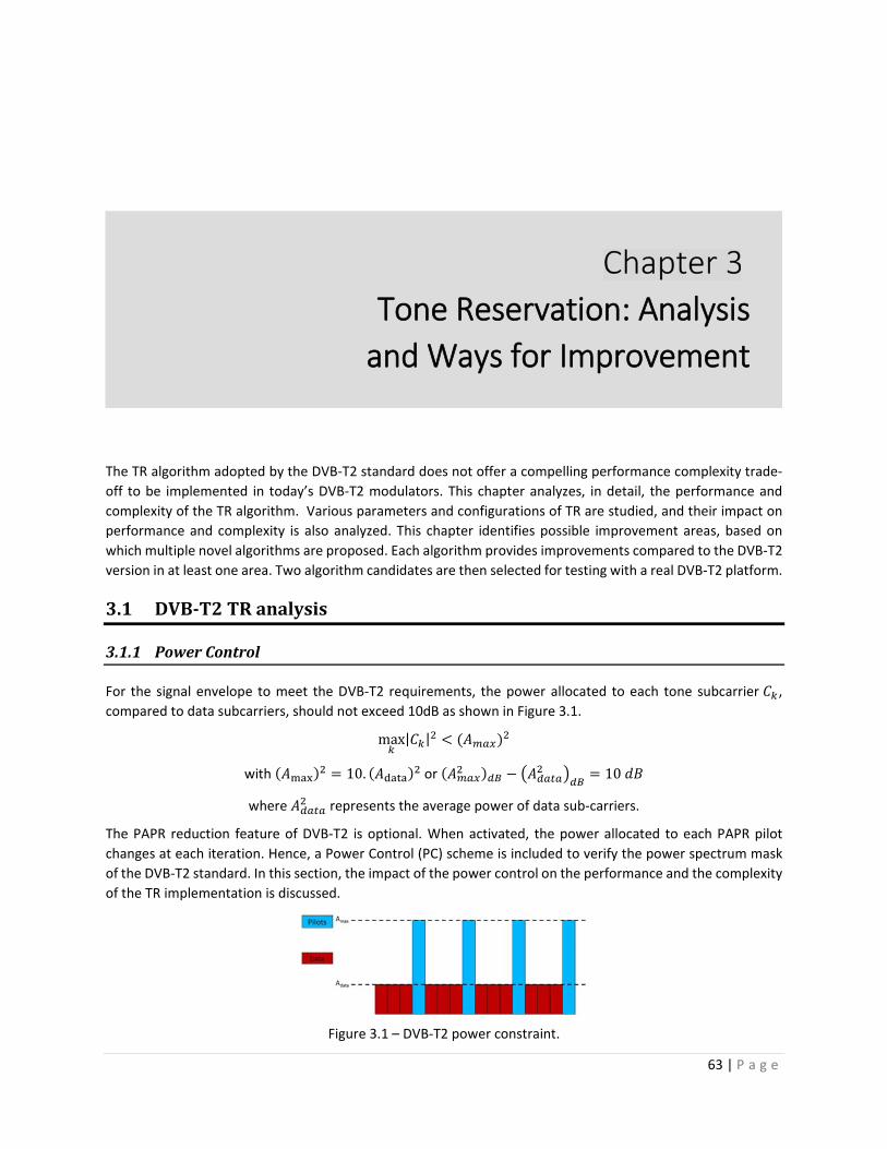
63 | P a g e
Tone Reservation: Analysis
and Ways for Improvement
The TR algorithm adopted by the DVB‐T2 standard does not offer a compelling performance complexity trade‐
off to be implemented in today’s DVB‐T2 modulators. This chapter analyzes, in detail, the performance and
complexity of the TR algorithm. Various parameters and configurations of TR are studied, and their impact on
performance and complexity is also analyzed. This chapter identifies possible improvement areas, based on
which multiple novel algorithms are proposed. Each algorithm provides improvements compared to the DVB‐T2
version in at least one area. Two algorithm candidates are then selected for testing with a real DVB‐T2 platform.
3.1 DVB‐T2TRanalysis
3.1.1 PowerControl
For the signal envelope to meet the DVB‐T2 requirements, the power allocated to each tone subcarrier ,
compared to data subcarriers, should not exceed 10dB as shown in Figure 3.1.
max| |
with 10. or 10
where represents the average power of data sub‐carriers.
The PAPR reduction feature of DVB‐T2 is optional. When activated, the power allocated to each PAPR pilot
changes at each iteration. Hence, a Power Control (PC) scheme is included to verify the power spectrum mask
of the DVB‐T2 standard. In this section, the impact of the power control on the performance and the complexity
of the TR implementation is discussed.
Figure 3.1 – DVB‐T2 power constraint.

64 | P a g e
3.1.1.1 Reserved Tones Power build up
At the end of each iteration, an adjusted version of the kernel is added to the signal in time domain. In frequency
domain, only the reserved tones are affected. If the OFDM carriers carried only real values, the power constraint
can easily be respected by equally dividing the available power among the iterations. However, the symbols
carry complex values, both the kernel samples and the signal samples can be represented by complex vector.
The amplitude of their sum is smaller or equal than the sum of their amplitudes, thus the contributions are not
the same for every iteration. Figure 3.2 shows the power build‐up for the reserved tones and displays the
contribution of each iteration in a different color. For a given reserved sub‐carrier the amount of power can
either grow or shrink after each iteration.
In the next paragraphs two different techniques to control the power allocated by the TR algorithm are detailed.
After 1st iteration After 2nd iteration
After 3rd iteration
Figure 3.2 – Power build up.
3.1.1.2 Power control per symbol
Early releases of the DVB‐T2 standard [147] did not specify a power control scheme implementation. A straight
forward approach is to allow the TR algorithm to complete (i.e. execute all iterations) for a given OFDM symbol
(hence the name per symbol) and then clip the amplitude of the subcarriers not meeting the power constraint
(see Figure 3.3) . This power control scheme is referred to as PC=SYMB.
Since the peak reduction process is executed in time domain and the power control constraint is defined for
each subcarrier in frequency domain, PC=SYMB requires an additional IFFT to be computed.
Figure 3.3 – Power build up for PC=SYMB.

65 | P a g e
3.1.1.3 Power control per iteration
The processing of an OFDM symbol, including PAPR reduction, must be completed before the next symbol is
received. This makes it very challenging to fit in an additional IFFT (in addition to the IFFT required by OFDM) for
power control purposes.
To avoid this, the last version of the DVB‐T2 standard [38] specifies a power control scheme that keeps track,
iteration by iteration, of the allocated power for each reserved subcarrier and allocates power in a way that no
tones exceed the threshold.
The amount of amplitude scaling, , that can be applied to the kernel at iteration without the tth reserved
tone exceeding the power limit is computed as follows:
where, : position of the peak being processed
∅: phase of the peak being processed
: value of the tth reserved tone after the previous iteration (Build‐up pilot)
: Square root of the maximum available power per tone
The geometric explanation of the above equations is shown in Figure 3.4. It consists of finding the , in such a
way that the resulting amplitude of the sum of the build‐up pilot and current pilot is equal to .
Figure 3.4 – DVB‐T2 power control (1).
is computed for every reserved tone. The amount of scaling that can be performed without violating the
power constraint is equal to .
…
Reserved Tone 1 Reserved Tone 2 Reserved Tone M
Figure 3.5 – DVB‐T2 power control (2).
10. . ∅
∗. ∗. : (3.1)
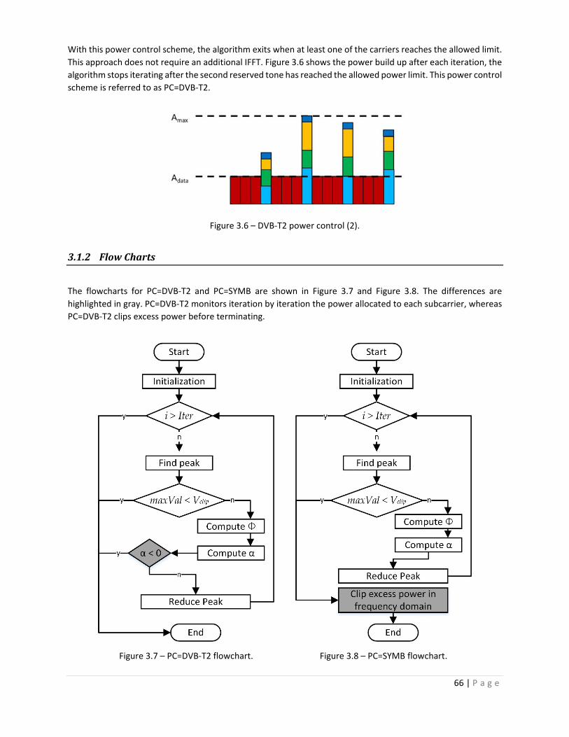
66 | P a g e
With this power control scheme, the algorithm exits when at least one of the carriers reaches the allowed limit.
This approach does not require an additional IFFT. Figure 3.6 shows the power build up after each iteration, the
algorithm stops iterating after the second reserved tone has reached the allowed power limit. This power control
scheme is referred to as PC=DVB‐T2.
Figure 3.6 – DVB‐T2 power control (2).
3.1.2 FlowCharts
The flowcharts for PC=DVB‐T2 and PC=SYMB are shown in Figure 3.7 and Figure 3.8. The differences are
highlighted in gray. PC=DVB‐T2 monitors iteration by iteration the power allocated to each subcarrier, whereas
PC=DVB‐T2 clips excess power before terminating.
Figure 3.7 – PC=DVB‐T2 flowchart.
Figure 3.8 – PC=SYMB flowchart.

67 | P a g e
3.1.2.1 Comparison
This section compares the performance of the two power control schemes PC=SYMB and PC=DVB‐T2. For a
MER= ‐40 dB, the performance difference in terms of IBO gain is 0.2 dB in 2K mode (Figure 3.9) and 0.37 dB in
32K mode (Figure 3.10), which leads to the saving of a lot of energy with DVB HPA since the power transmitted
is usually very large (in the order of tens kWatts).
Figure 3.9 – MER 2K.
Figure 3.10 – MER 32K.
The performance difference in terms of PAPR gain at CCDF=10‐3 is 0.4 dB in 2K mode (Figure 3.11) and 0.7dB in
32K mode (Figure 3.12). PC=SYMB outperforms PC=DVB‐T2 in both MER and CCDF metrics. However, it requires
an additional IFFT to be computed for each OFDM symbol, which is costly in terms of resource usage and causes
additional processing delays especially in 32K mode.
Figure 3.11 – CCDF 2K.
Figure 3.12 – CCDF 32K.
3.1.3 Algorithm
This section describes the TR algorithm as described in the DVB‐T2 standard, this algorithm is used as a base for
our proposed methods. Table 3.1 includes the parameters required to define the TR algorithm. The differences
between the two power control techniques can be seen in step 6 and step 13.

68 | P a g e
Table 3.1 – Tone reservation algorithm parameters
Name Description Example
Current iteration count
Maximum number of iterations 30
Positions of the M dedicated pilots according to DVB‐T2 standard 18
The set of dedicated pilots …
Maximum available power per tone according to DVB‐T2 standard 10dB
Amplitude threshold 7.2dB
The power control scheme used. DVB_T2: according to the DVB‐T2 standard SYMB: removing excess power at the end of the algorithm
Let be the time domain version of the OFDM signal
1. /
1. Initialization
a. Initialize the iteration count
1 b. pre‐compute kernel and store in memory
c k1
∈
, ∈ 0… 1
c. initialize the reduction signal
0, ∈ 0… 1
2. Check if the maximum number of iterations has been reached
11 3. Find the maximum to reduce
| | | |
4. Check if signal verifies threshold condition
11 5. Calculate correction Phase
∅ 6. Power control
a. If _ 2, calculate available power per reserved tone and deduce power factor
10. . ∅
∗. ∗.
min0
,
b. If , calculate power factor
0
7. Update reserved tones
. . ∅

69 | P a g e
8. Reduce peak
. ∅. 9. Increment iteration count
10. Reiterate
2 11. Finish iterations
12. IF _ 2, compute output
13. IF
a. Truncate additional power
,
. . ,
b. Compute output
0
3.1.4 ImpactoftheClippingThreshold
In TR algorithm, the clipping threshold ( ) has two roles: it specifies the amount of peak reduction to
perform, and is used as an exit condition. In fact, at each iteration the TR algorithm searches for the highest
signal peak. If the amplitude of the highest signal peak is greater than , the algorithm exits. If not the
algorithms aims at reducing the highest peak amplitude to match by adding an adjusted version of the
kernel.
The MER performance for different values of is shown in Figure 3.13. Decreasing the value of
increases both the number of peaks being reduced (more peaks fall above the threshold) and the amount of
peak reduction being performed, which explains the better performance.
It can also be noticed from this figure that for values of smaller than 7.2dB, the improvements are
negligible. For such low values, a considerable number of additional peaks falls above the threshold, given the
limited number of available iterations, not all of them can be targeted by the peak reduction process. In this
study the threshold is set to 7.2 dB for all OFDM symbols. In paragraph 3.3.1, a technique that dynamically
optimizes the clipping threshold for each symbol is presented.
Figure 3.13 – Variable clip value for PC=SYMB 2K with 30 iterations.

70 | P a g e
3.1.5 ReservedTonesandKernelGeneration
The DVB‐T2 standard allocates almost one percent of the available subcarriers to be used by the TR PAPR
reduction algorithm. Table 3.2 contains the number of reserved tones for different OFDM symbol sizes according
to the DVB‐T2 standard.
Table 3.2 – Number of reserved tones for different OFDM modes in DVB‐T2.
Mode 1K 2K 4K 8K 16K 32K
Number of reserved tones 9 18 36 72 144 288
The positions of the reserved tones for P2 and frame closing symbols are provided in Annex A. For data symbols,
the positions of the reserved tones vary based on the scattered pilot pattern used. For a data symbol in a
frame, the reserved tones set is determined as follows:
⟨ ⟩, ∈ , (3.2)
where, : is the number of P2 symbols in one frame,
: denotes the set of reserved carriers corresponding to carrier indices defined in Annex A, and
: is the number of symbols in the frame excluding P1, P2 or any frame closing symbol
It can be seen from (3.2) that the positions of the reserved tones are not the same for all OFDM symbols. In fact
the reserved tones are circularly shifted from one symbol to another. The amount of circular shift depends on
the pilot pattern used (see paragraph 1.3.6). The kernel signal is obtained by IFFT after setting the reserved
carriers to 1 and the remaining carriers to 0. Thus, the obtained kernel is different from one symbol to another.
The number of different kernels required for each pilot pattern is displayed in Table 3.3.
Table 3.3 – Pilot Patterns in DVB‐T2 for data symbols.
Pilot Pattern 1 2 3 4 5 6 7 8
Number of different kernels 4 2 4 2 4 2 4 16
At each iteration of TR, the corresponding kernel, is scaled, shifted and its phase adjusted to perform peak
reduction. The time domain representations of the kernels have the same length as the OFDM signal and can
either:
be generated at runtime, when needed: this requires an additional IFFT to be performed for each
symbol, which is costly in hardware resource utilization and in processing delay, or
be pre‐computed and stored in memory: this requires a huge amount of memory. For a Xilinx Virtex 6
VLX95T FPGA, storing the 16 kernels for a PP8 pattern in 32K mode would require 18,874,368 bits (32678
samples x 18 bits per sample x 16 kernels x 2 for real and imaginary parts). This will consume 48% more
than the total available RAMB36E1.
When TR is used by the modulator at the transmitter side, the reserved tones must be ignored by the receiver.
The receiver is informed via L1 pre‐signaling when TR is activated
3.1.6 ImpactofOversampling
Reducing the highest peak of the discrete‐time signal does not necessarily reduce the PAPR of the analog signal.
In fact analog signal peaks can occur between the digital samples. An upsampled version of the discrete signal
can be used to offer better peak reduction accuracy; the TR algorithm is then used to reduce the peaks of the
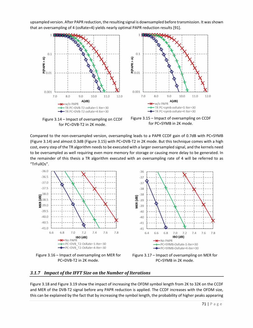
71 | P a g e
upsampled version. After PAPR reduction, the resulting signal is downsampled before transmission. It was shown
that an oversampling of 4 (osRate=4) yields nearly optimal PAPR reduction results [91].
Figure 3.14 – Impact of oversampling on CCDF for PC=DVB‐T2 in 2K mode.
Figure 3.15 – Impact of oversampling on CCDF for PC=SYMB in 2K mode.
Compared to the non‐oversampled version, oversampling leads to a PAPR CCDF gain of 0.7dB with PC=SYMB
(Figure 3.14) and almost 0.3dB (Figure 3.15) with PC=DVB‐T2 in 2K mode. But this technique comes with a high
cost, every step of the TR algorithm needs to be executed with a larger oversampled signal, and the kernels need
to be oversampled as well requiring even more memory for storage or causing more delay to be generated. In
the remainder of this thesis a TR algorithm executed with an oversampling rate of 4 will be referred to as
“TrFullOs”.
Figure 3.16 – Impact of oversampling on MER for PC=DVB‐T2 in 2K mode.
Figure 3.17 – Impact of oversampling on MER for PC=SYMB in 2K mode.
3.1.7 ImpactoftheIFFTSizeontheNumberofIterations
Figure 3.18 and Figure 3.19 show the impact of increasing the OFDM symbol length from 2K to 32K on the CCDF
and MER of the DVB‐T2 signal before any PAPR reduction is applied. The CCDF increases with the OFDM size,
this can be explained by the fact that by increasing the symbol length, the probability of higher peaks appearing
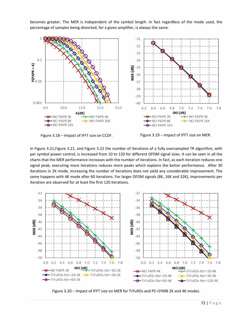
72 | P a g e
becomes greater. The MER is independent of the symbol length. In fact regardless of the mode used, the
percentage of samples being distorted, for a given amplifier, is always the same.
Figure 3.18 – Impact of IFFT size on CCDF.
Figure 3.19 – Impact of IFFT size on MER.
In Figure 3.21,Figure 3.21, and Figure 3.22 the number of iterations of a fully oversampled TR algorithm, with
per symbol power control, is increased from 10 to 120 for different OFDM signal sizes. It can be seen in all the
charts that the MER performance increases with the number of iterations. In fact, as each iteration reduces one
signal peak, executing more iterations reduces more peaks which explains the better performance. After 30
iterations in 2K mode, increasing the number of iterations does not yield any considerable improvement. The
same happens with 4K mode after 60 iterations. For larger OFDM signals (8K, 16K and 32K), improvements per
iteration are observed for at least the first 120 iterations.
Figure 3.20 – Impact of IFFT size on MER for TrFullOs and PC=SYMB 2K and 4K modes.

73 | P a g e
Figure 3.21 – Impact of IFFT size on MER for TrFullOs and PC=SYMB 8K and 16K modes.
Figure 3.22 – Impact of IFFT size on MER for TrFullOs and PC=SYMB 32K mode.
The graphs in Figure 3.23, show that in order to maintain the same MER performance, when increasing the
OFDM symbol length from L1 to L2, the number of iterations must be increased by a factor of L2/L1. For example,
30 iterations with a signal of length 2K yield the same MER performance as 120 (4x30) iterations with a signal of
length 8K (4x2K).
This is important because it shows that to maintain a target MER for longer symbols the number of TR iterations
needs to be increased significantly. Each TR iteration traverses the signal at least one time to detect the peak to
be reduced, this operation consumes at least 32K processor clock ticks which is the same as the duration of the
32K OFDM signal. A commercial DVB‐T2 modulator using Xilinx Vertex 6 can afford to allocate only 8 to 10 times
the duration of an OFDM symbol for PAPR reduction techniques. Just considering the peak detection step, this

74 | P a g e
limits to roughly 10 iterations the actual number of iterations that can be executed without incurring the cost
of upgrading to a faster hardware platform.
Figure 3.23 – Relation between IFFT size and required number of iterations for TrFullOs and PC=SYMB.
3.1.8 ImpactofthePowerControlontheNumberofExecutedIterations
The previous section presented the impact on increasing the number of iterations for PC=SYMB. MER
performance charts of PC=DVB‐T2, for various iteration count and symbol sizes, are displayed in Figure 3.24. It
is clear that increasing the number of iterations does not yield additional performance.
To better understand the reason of this behavior, the average number of iterations being executed and the
average percentage of pilot power usage are displayed, side by side for PC=DVB‐T2 and PC=SYMB, for various
OFDM symbol sizes in Table 3.4, Table 3.5 and Table 3.6. Whereas PC=SYMB consumes almost all the available
iterations, PC=DVB‐T2 exits earlier and uses only 5.84 iterations in 2K mode, 6.1 in 8K mode and 9.64 in 32K
mode. PC=DVB‐T2 algorithm exits when:
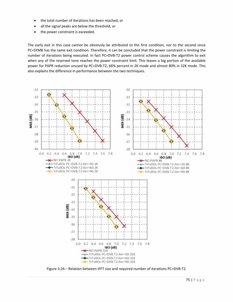
75 | P a g e
the total number of iterations has been reached, or
all the signal peaks are below the threshold, or
the power constraint is exceeded.
The early exit in this case cannot be obviously be attributed to the first condition, nor to the second since
PC=SYMB has the same exit condition. Therefore, it can be concluded that the power constraint is limiting the
number of iterations being executed. In fact PC=DVB‐T2 power control scheme causes the algorithm to exit
when any of the reserved tone reaches the power constraint limit. This leaves a big portion of the available
power for PAPR reduction unused by PC=DVB‐T2, 66% percent in 2K mode and almost 80% in 32K mode. This
also explains the difference in performance between the two techniques.
Figure 3.24 – Relation between IFFT size and required number of iterations PC=DVB‐T2.

76 | P a g e
Table 3.4 – Iteration statistics 2K.
TrFullOs TrFullOs TrFullOs TrFullOs TrFullOs TrFullOs
Iterations 30 60 90 30 60 90
Power Control DVB‐T2 DVB‐T2 DVB‐T2 SYMB SYMB SYMB
Avg. Number of iterations 5.84 5.84 5.84 29.88 59.58 89.28
Average Pilot power usage 43.22% 43.22% 43.22% 62.74% 67.88% 69.67%
Table 3.5 – Iteration statistics 8K.
TrFullOs TrFullOs TrFullOs TrFullOs TrFullOs TrFullOs
Iterations 30 60 90 30 60 90
Power Control DVB‐T2 DVB‐T2 DVB‐T2 SYMB SYMB SYMB
Avg. Number of iterations 6.1 6.1 6.1 30 60 90
Average Pilot power usage 30.22% 30.22% 30.22% 53.45% 59.54% 62.80%
Table 3.6 – Iteration statistics 32K.
TrFullOs TrFullOs TrFullOs TrFullOs TrFullOs TrFullOs
Iterations 30 60 90 30 60 90
Power Control DVB‐T2 DVB‐T2 DVB‐T2 SYMB SYMB SYMB
Avg. Number of iterations 9.64 9.64 9.64 30 60 90
Average Pilot power usage 20.54% 20.54% 20.54% 39.66% 47.23% 51.19%
3.1.9 ImpactofHPALinearity
The MER performance for TrFullOs for various knee factor p of the Rapp model are illustrated in Figure 3.25. It
can be seen that when the HPA is more linear, i.e. when increases, the MER gain increases as well. For p=3,
the simulated amplifier has strong nonlinear transfer function and the MER gain of TrFullOs is small. The MER
gain is much higher for 10and 100.
Figure 3.25 – Impact of HPA non linearity on TR algorithm, 32K mode.

77 | P a g e
While a value of 3 for is typical to model an HPA alone, in this study is set to 10. This is to model the HPA
operating with a predistortion module as used in the real platform developed with project’s partners and
described in section 4.3.
3.1.10 SOCP
A comparison between the optimal solution SOCP (see paragraph 2.3.8.2) and TR techniques are shown in Figure
3.26 without power control and in Figure 3.27 with power control per symbol. The impact of power control can
be noticed by comparing the two graphs. Without power control, SOCP leads to a gain of more than 0.6 dB.
However this gain drops to 0.2 dB when power control per symbol is used. This further highlights the impact of
power control on PAPR reduction performance.
Figure 3.26 – CCDF for SOCP and TR without power control (PC=NO).
Figure 3.27 – CCDF for SOCP and TR with PC=SYMB.
Figure 3.28 displays the CCDF performance of SOCP without oversampling and with an oversampling rate of 4.
It can be seen that oversampling yields to a PAPR CCDF gain of 1.7 dB.

78 | P a g e
Figure 3.28 – Impact of oversampling on CCDF for SOCP with PC=SYMB.
This paragraph highlights the importance of oversampling and shows how power control can have a negative
impact on optimization techniques. These points will be taken into consideration when introducing new PAPR
reduction techniques in the next chapters.
3.1.11 LimitationsandDrawbacksoftheDVB‐T2TRAlgorithm
This section analyzed various aspects of the TR algorithm adopted in the DVB‐T2 standard. Table 3.7 includes a
summary of possible areas of improvements. These areas are targeted in the next sections to propose novel
solutions that provide a good performance/complexity tradeoff.
Table 3.7 – Analysis summary
Area Conclusion
Kernels Kernel generation and storage are factor of complexity
Oversampling Oversampling can bring performance improvement but requires too much resources
Clipping threshold
The clip value is not optimized for each OFDM symbol
Iteration count
In order to achieve acceptable PAPR reduction, the number of iterations needs to be considerably increased especially in 32K mode, but in practice only 8 to 10
total peaks can be performed with reasonable processing delay
Power control
The power control scheme used in DVB‐T2 does not take advantage of all available power, more power can be used to achieve better performance
3.2 PartialOversamplingandFractionalShiftedKernels
The Partial Oversampled Fractional Shifted (POFSK) algorithm takes advantage of the precision provided by
oversampling the time domain signal (see paragraph 3.1.6) without having to oversample the complete symbol
and without having to execute the complete algorithm in an oversample mode.

79 | P a g e
3.2.1 PartialOversampling
Instead of oversampling the complete input sequence, we decide to compute only 4 additional oversampled
samples as follows:
1‐ find the maximum position ( ) and value ( ) of the non‐oversampled input (as in
standard TR algorithm),
2‐ compute the 2 oversampled samples preceding the maximum position,
3‐ compute the 2 oversampled samples following the maximum position.
So instead of computing all the oversampled samples (in red in Figure 3.29), we only compute the 4 oversampled
samples (in yellow in Figure 3.30) surrounding the maximum of the sequence.
Figure 3.29 – Completely oversampled signal
Figure 3.30 – Partially oversampled signal.
The computation can be executed by convoluting the input of the algorithm and 1/ / (low pass
filtering operation), the convolution does not have to be computed for all the samples, only for the chosen ones.
Different types of low pass filters, less complex than the cardinal since convolution, can also be considered.
Instead of using and of the non‐oversampled input for the next steps of the TR algorithm, the
maximum among and the 4 calculated oversampled values is computed and used in the next algorithm
steps. This new maximum is referred to as oversampled maximum.
3.2.2 FractionalShiftedPilots
In DVB‐T2 TR, once the maximum position is calculated, a circular shift is applied to the reference kernel in order
for its maximum to coincide with the maximum of the sequence. The challenge with the partial oversampled
sequence, is how to circularly shift a non‐oversampled kernel to the oversampled maximum position. For this
we propose to use 4 additional versions of that kernel defined as follows:
11, ∈
0,
1 2 1 . /
1 1 1 . / 1 1 1 . /
1 2 1 . /
Those kernels are referred to as Fractional Shifted Kernels (FSK). Compared to the 1TR standard kernel, which
has a maximum for k=0, those kernels have maximums when oversampled at the positions shown in Table 3.8.
Table 3.8 – Peak position of fractional shifted kernels.
Peak position ‐ not oversampled Peak position ‐ oversampled

80 | P a g e
1TR 0 0 1TR2A 0 2 1TR1A 0 1 1TR1B 0 R.N‐1 1TR2B 0 R.N‐2
The choice of the kernel to be used for the next steps of the TR algorithm depends on the position of the
recalculated oversampled maximum (see Figure 3.31), i.e. if the oversampled maximum is at 2B then 1TR2B is
used.
Figure 3.31 – Kernel choice.
Similar to PC=DVB‐T2, the 1TR kernel can either be generated in real‐time or stored in memory. However the
new kernels (1TR2A, 1TR1A, 1TR1B and 1TR2B) can be generated from 1TR using a simple phase shift, and thus
can be computed at run time. Compared to TrFullOs, which has to deal with oversampled kernels, POFSK deals
with one non‐oversampled kernel and can quickly generate (without any IFFT) the fractional shifted kernels at
runtime.
3.2.3 POFSKPerformance
Figure 3.32 displays the CCDF performance for TR and POFSK for different iteration counts. POFSK achieves,
regardless of the number of iterations, an additional gain of 0.2 dB at CCDF 10‐3 compared to PC=SYMB.

81 | P a g e
Figure 3.32 – CCDF comparison for TR and POFSK, 2K mode.
3.2.4 GeneralizedPartialOversampledandFractionalShiftedKernels
The same logic of partial oversampling and shifted fractional kernels can be generalized. Instead of only
computing the 4 oversampled samples surrounding the non‐oversampled maximum position, the Generalized
POFSK (GPOFSK) computes 2 surrounding samples for each of the highest signal
peaks to create a set from which the oversampled maximum is chosen. Examples of possible combinations are
shown in Figure 3.33 and Figure 3.34).
Figure 3.33 – Partial oversampled signal with 2 and 3
Figure 3.34 – Partial oversampled signal with 3 and 1
The GPOFSK techniques is equivalent to:
TR, when 1 and 0 POFSK, when 1 and 2 TrFullOs, when and 3
3.2.5 Algorithm
In addition to the parameters defined for TR, GPOFSK requires the definition of additional parameters listed in
Table 3.9. Most of the operations are similar to the DVB‐T2 standard. The main difference can be noticed in
step1, step 3 and step 5. In step 1, the fractional kernels are computed and stored in memory. In step 3.a, the
algorithm computes the highest peaks of the non‐oversampled signal. Then in step 3.b, GPOFSK
performs oversampling only around the previously detected peaks. The detected peaks and the additional
samples computed around them are then used in 3.c to find the maximum to be reduced. In step 5, the position

82 | P a g e
of the maximum is used to determine the corresponding fractional kernel. This fractional kernel is then scaled,
circularly shifted and adjusted, as in TR, to reduce the amplitude of the detected maximum.
Table 3.9 – GPOFSK additional parameters.
Name Description Notes
Number of samples to compute per peak 2
Number of additional peaks to consider
oversampling rate used 4
The following algorithm defines the steps required to execute GPOFSK, which uses fractional kernels to avoid
the execution of the algorithm in oversampled mode (check steps 1.b and 5).
Let be the time domain version of the OFDM signal
1. /
1. Initialization
a. Initialize the iteration count: 1b. Pre‐compute the fractional kernels and store in memory :
1 . .
∈
, ∈ 0, 1 ∈ …
c. Initialize the reduction signal
0, ∈ 0, 1
2. Check if the maximum number of iterations has been reached
13
3. Find the maximum to reduce
a. Calculate the highest amplitudes of
0, ∈ 0; 1 0, ∈ 0; 1
| |,
b. Apply partial oversampling to positions around
0, ∈ 0; . 1
, ,
c. Find oversampled maximum
| | | | / 2. 1
4. Check if signal verifies threshold condition
∅
13
5. Chose appropriate kernel
2. 1 2 6. Calculate correction Phase
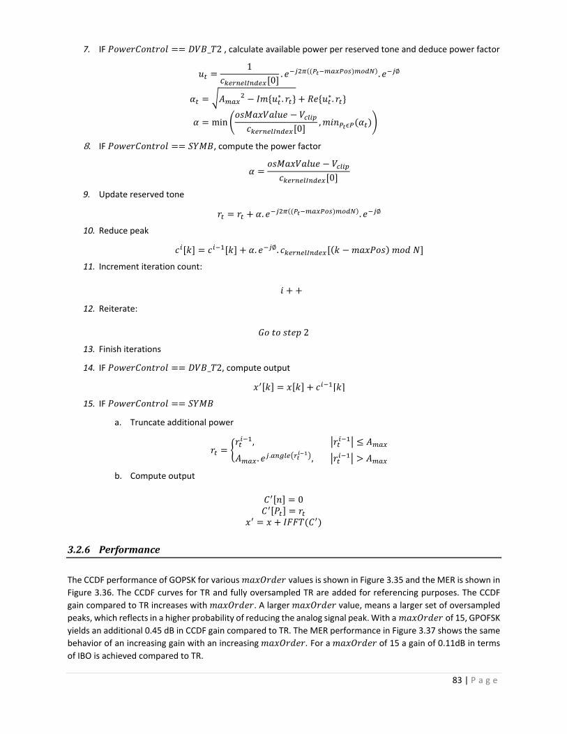
83 | P a g e
7. IF _ 2 , calculate available power per reserved tone and deduce power factor
10. . ∅
∗. ∗.
min0
,
8. IF , compute the power factor
0
9. Update reserved tone
. . ∅
10. Reduce peak
. ∅.
11. Increment iteration count:
12. Reiterate:
2
13. Finish iterations
14. IF _ 2, compute output
15. IF
a. Truncate additional power
,
. . ,
b. Compute output
0
3.2.6 Performance
The CCDF performance of GOPSK for various values is shown in Figure 3.35 and the MER is shown in
Figure 3.36. The CCDF curves for TR and fully oversampled TR are added for referencing purposes. The CCDF
gain compared to TR increases with . A larger value, means a larger set of oversampled
peaks, which reflects in a higher probability of reducing the analog signal peak. With a of 15, GPOFSK
yields an additional 0.45 dB in CCDF gain compared to TR. The MER performance in Figure 3.37 shows the same
behavior of an increasing gain with an increasing . For a of 15 a gain of 0.11dB in terms
of IBO is achieved compared to TR.

84 | P a g e
Figure 3.35 – CCDF for GPOSK with variable , 2, PC=SYMB, 10 and mode 2K.
Figure 3.36 – MER for GPOSK with variable , 2, PC=SYMB, 10 and mode 2K.
With only 10 iterations, GPOFSK increases the performance of TR towards those of a fully oversampled TR
algorithm. The IBO gain can be further increased with more iterations. Figure 3.37 shows that a gain of 0.3dB in
IBO, compared to TR, can be achieved with 30 iterations.

85 | P a g e
Figure 3.37 – MER for GPOSK with variable , 2, PC=SYMB, 30 and mode 2K.
3.3 DynamicThresholdandEnhancedPeakSelection
The GPOFSK technique improves the performance of a non‐oversampled TR algorithm towards those of an
oversampled one. GPOFSK takes advantage of the oversampling precision without requiring the oversampling
of the signal and kernel.
However, to be effective GPOFSK, must be combined with PC=SYMB (it was shown in paragraph 3.1.6, when
PC=DVB‐T2 is used, that the CCDF gain of a fully oversampled TR is only 0.3dB compared to the standard TR).
The use of PC=SYMB requires an additional IFFT to be computed for each symbol, which is computationally
costly.
In this section, two techniques are introduced in order to enhance the performance of PC=DVB‐T2 towards those
of PC=SYMB without the use of any IFFT. The first technique is based on a dynamic computation of the clipping
threshold and the second enhances the selection of the peaks to be reduced in such a way to achieve better
performance.
3.3.1 DynamicThreshold
The TR algorithm is designed to reduce one signal peak per iteration. In an ideal scenario, where no peak
regrowth occurs and no power constraint has to be respected, the best that can be achieved is the reduction of
a number of peaks equal to the number of maximum available iterations ( ). For the same ideal scenario, the
amplitude of the highest peak at the end of the algorithm execution is equal to the 1 highest peak
amplitude before the execution of the algorithm, since the first peaks would have been reduced.
When is set to a value higher than the amplitude of the 1 initial peak, it translates into less PAPR
reduction performance, since too few peaks are targeted by PAPR reduction (Figure 3.38).
Figure 3.38 – High value.
If is set to the amplitude of the 1 initial peak, the ideal algorithm reduces the amplitude of the
first peaks to match the amplitude of the 1 initial peak (Figure 3.39).
Figure 3.39 – set to the amplitude of the 1 initial peak with 4.
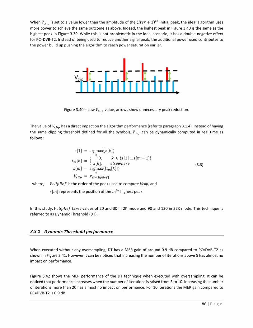
86 | P a g e
When is set to a value lower than the amplitude of the 1 initial peak, the ideal algorithm uses
more power to achieve the same outcome as above. Indeed, the highest peak in Figure 3.40 is the same as the
highest peak in Figure 3.39. While this is not problematic in the ideal scenario, it has a double‐negative effect
for PC=DVB‐T2. Instead of being used to reduce another signal peak, the additional power used contributes to
the power build up pushing the algorithm to reach power saturation earlier.
Figure 3.40 – Low value, arrows show unnecessary peak reduction.
The value of has a direct impact on the algorithm performance (refer to paragraph 3.1.4). Instead of having
the same clipping threshold defined for all the symbols, can be dynamically computed in real time as
follows:
1 argmax
0, ∈ 1 … 1
,
argmax | |
(3.3)
where, is the order of the peak used to compute Vclip, and
represents the position of the highest peak.
In this study, takes values of 20 and 30 in 2K mode and 90 and 120 in 32K mode. This technique is
referred to as Dynamic Threshold (DT).
3.3.2 DynamicThresholdperformance
When executed without any oversampling, DT has a MER gain of around 0.9 dB compared to PC=DVB‐T2 as
shown in Figure 3.41. However it can be noticed that increasing the number of iterations above 5 has almost no
impact on performance.
Figure 3.42 shows the MER performance of the DT technique when executed with oversampling. It can be
noticed that performance increases when the number of iterations is raised from 5 to 10. Increasing the number
of iterations more than 20 has almost no impact on performance. For 10 iterations the MER gain compared to
PC=DVB‐T2 is 0.9 dB.

87 | P a g e
Figure 3.41 – TR with Dynamic Threshold and 20 and variable number of iterations, mode 2K.
Figure 3.42 – TrFullOs with Dynamic Threshold and =20 and variable number of iterations, mode 2K.
3.3.3 EnhancedPeakSelection
The Enhanced Peak Selection (EPS) algorithm modifies the TR algorithm adopted in DVB‐T2 to allow for the
execution of more iterations. When any of the reserved tones for PAPR reduction in a PC=DVB‐T2 algorithm
reaches the power constraint the algorithm terminates. At that point the reduction of the current peak would
have caused the allocated power to exceed the permissible limit.
Instead of exiting the algorithm at this stage, the peak causing the algorithm to terminate is added by PC=EPS
to a “skip list”. Then, PC=EPS executes an additional iteration, this time excluding the recorded peak positions
in the “skip list” from the peak search candidates. This process is repeated for every peak whose reduction
violates the power constraint.
Figure 3.43 illustrates, side by side, the evolution of the signal peaks (in time domain) and the pilot’s power (in
frequency domain) for 4 iterations of PC=EPS. The circle indicates the current peak targeted by the algorithm.
Two peaks are successfully reduced in the 1st and 2nd iterations, however the peak targeted by the 3rd iteration
would cause the power limit to be exceeded. This peak is added to the “skip list,” and the 4th iteration excludes

88 | P a g e
this peak, in green, from its peak search. The 4th iteration targets another peak whose reduction respects the
power constraint. For the same scenario PC=DVB‐T2 would have executed two iterations only, reduced two
peaks and exited on the third iteration.
Iteration Time domain Frequency domain
1st
2nd
3rd
4th
Figure 3.43 – EPS iteration details.
3.3.4 Algorithm
The flow chart of the proposed EPS and DT techniques is shown in Figure 3.44. The differences with PC=DVB‐T2
are highlighted in gray.
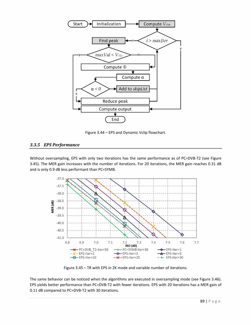
89 | P a g e
Figure 3.44 – EPS and Dynamic Vclip flowchart.
3.3.5 EPSPerformance
Without oversampling, EPS with only two iterations has the same performance as of PC=DVB‐T2 (see Figure
3.45). The MER gain increases with the number of iterations. For 20 iterations, the MER gain reaches 0.31 dB
and is only 0.9 dB less performant than PC=SYMB.
Figure 3.45 – TR with EPS in 2K mode and variable number of iterations.
The same behavior can be noticed when the algorithms are executed in oversampling mode (see Figure 3.46).
EPS yields better performance than PC=DVB‐T2 with fewer iterations. EPS with 20 iterations has a MER gain of
0.11 dB compared to PC=DVB‐T2 with 30 iterations.

90 | P a g e
Figure 3.46 – TrFullOs with EPS in 2K mode and variable number of iterations.
3.3.6 PerformanceofEPSandDTCombined
The EPS technique can be easily combined with the DT technique. The MER performance results for both 2K
mode and 32K mode are shown in Figure 3.47 and Figure 3.48. With 20 iterations EPS‐DT outperforms PC=DVB‐
T2 with 30 iterations by 0.2 dB in 2K mode. And in 32K, the gain is 0.36 dB for the same number of iterations.
Figure 3.47 – TrFullOs with EPS‐DT in 2K mode and =20.

91 | P a g e
Figure 3.48 – TrFullOs with EPS‐DT in 32K mode and =120.
EPS, DT and EPS‐DT increase the performance of PC=DVB‐T2 towards PC=SYMB without requiring any additional
IFFT to be computed. Table 3.10 compares the number of iterations and the pilot power usage of various EPS‐
DT configurations and PC=SYMB and PC=DVB‐T2. It can be seen that EPS‐DT allows the algorithms to execute
more iterations (79.4 out of 90 compared to 9.6 out of 90 for PC=DVB‐T2). EPS‐DT has a better power usage; for
90 iterations EPS‐DT allocates only 17.9% of the available pilot power compared to 20.5% for PC=DVB‐T2 while
providing better performance.
Table 3.10 – Actual power allocated and iterations executed for different configurations for 32K mode
32k mode DVB_T2 EPS‐DT EPS‐DT EPS_DT SYMB
Vclip / VclipRef 7.2dB 120 120 120 7.2dB
Max. Iterations 90 30 60 90 90
Avg. # of iterations 9.6 29.3 56.5 79.4 90
Avg. Pilot power usage 20.5% 14.6% 16.7% 17.9% 51.2%
3.4 Conclusion
In this chapter a deep analysis of the TR algorithm adopted in DVB‐T2 was conducted. The analysis covered
multiple areas related to the power constraint imposed by the standard, the clipping threshold, the level of
oversampling, the algorithm exit conditions and the design of the kernel. It showed why the algorithm in the
DVB‐T2 standard is both costly to implement and poor in performance. The outcome of this analysis is then used
as a base to propose three novel algorithms: the Partial Oversampling and Fractional Shifted Kernels (POFSK)
technique is based on a partial oversampling of the signal in order to provide good PAPR reduction performance
without requiring the complete signal to be oversampled, the Dynamic Threshold (DT) technique allows for
better algorithm convergence by dynamically computing the PAPR reduction threshold for every OFDM symbol,
and the Enhanced Peak Selection (EPS) technique which provides additional PAPR reduction by choosing the
appropriate signal peaks to reduce and the peaks to skip. This chapter also presented simulation results of MER
and PAPR CCDF showing how the proposed techniques outperform the TR version of DVB‐T2.


93 | P a g e
Individual Carrier
Multiple Peaks
4.1 IndividualCarrierMultiplePeaks
The power control scheme PC=DVB‐T2 is designed to avoid the use of an additional IFFT for power control. This
leaves a part of the power allocated to PAPR reduction unused (see paragraph 3.1.8). The technique presented
in this section uses a new kernel definition and allocates power to the subcarriers individually in order to
maximize the power used for PAPR reduction.
4.1.1 Concept
As shown in paragraph 3.1.1, the PAPR reduction results can be strongly degraded depending on the power
control method. The proposed algorithm here is based on the concept of maximizing the utilization of the
available power for PAPR reduction. Each reserved tone is used once with maximum power during an iteration.
Thus, there is as many iterations as the number of reserved tones.
4.1.2 NewKernelDefinition
With Individual Carrier Single Peak ICSP, a different kernel is defined for every iteration , as follows:
0 (4.1)
where , defined in paragraph 3.1.5, is the position of the reserved tone corresponding to the current
iteration. The relation between the kernel definition and the iteration count is illustrated in Figure 4.1
The time domain version of the kernel is given by:
. ∅ .. .
, ∈ 0, 1 (4.2)
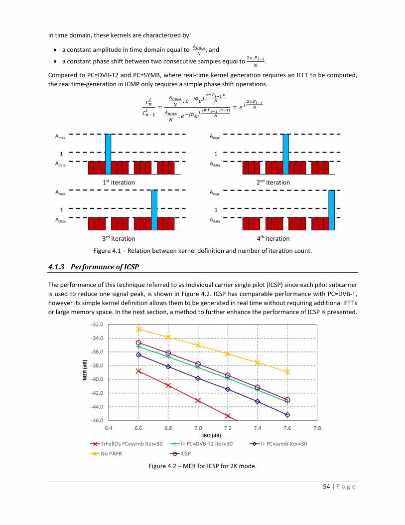
94 | P a g e
In time domain, these kernels are characterized by:
a constant amplitude in time domain equal to , and
a constant phase shift between two consecutive samples equal to .
.
Compared to PC=DVB‐T2 and PC=SYMB, where real‐time kernel generation requires an IFFT to be computed,
the real time‐generation in ICMP only requires a simple phase shift operations.
. ∅ .. .
. ∅ .. .
..
1st iteration 2nd iteration
3rd iteration 4th iteration
Figure 4.1 – Relation between kernel definition and number of iteration count.
4.1.3 PerformanceofICSP
The performance of this technique referred to as Individual carrier single pilot (ICSP) since each pilot subcarrier
is used to reduce one signal peak, is shown in Figure 4.2. ICSP has comparable performance with PC=DVB‐T,
however its simple kernel definition allows them to be generated in real time without requiring additional IFFTs
or large memory space. In the next section, a method to further enhance the performance of ICSP is presented.
Figure 4.2 – MER for ICSP for 2K mode.

95 | P a g e
4.1.4 PhaseOptimization
The PAPR reduction techniques discussed so far (PC=DVB‐T2, PC=SYMB, GPOFSK, ICSP) take into consideration
only the phase of one detected peak, i.e. the highest, to adjust the kernel phase∅. The main idea behind the
Individual Carrier Multiple Peaks (ICMP) technique is to target multiple peaks in one iteration. ICMP firstly
identifies the S highest peak amplitudes, then computes the correction phase∅, which minimizes the sum of the
squares of these peaks as follows:
∅ . ∅
∈
where, is the set of the highest peak positions of .
The problem turns out to find ∅ by deducing the derivative∅. Accordingly, we can write:
∅ . ∅ . ∅
∈
∅ . . . .∅ . .
∅
∈
∅ | | | | 2. . .∅
∈
The derivate with respect to ∅is given by:
∅2.
∅. .
∅
∈
∅2.
∅. ∅ . ∅
∈
∅2. . ∅ 2. . ∅
∅2. . sin ∅ 2 ,
where:
. .
∈
. .
∈
By solving∅
0 and studying the variation of∅, it can be show that ∅ has a minimum when:
∅32
2 , (4.3)

96 | P a g e
Compared to PC=DVB‐T2, the computation of ∅ in ICMP requires the pre‐computation and storage of
additional samples ( ) of the current kernel corresponding to the positions. However, the added complexity
is negligible:
can be computed by using a bubble sort algorithm to sort the input samples by amplitude (the
standard bubble sort algorithm requires the storage of the sorted array in memory. In the case of ICMP,
it is only necessary to store the top S samples). The bubble sort algorithm and the peak detection
performed by PC=DVB‐T2 both run in .
The value of S varies between 2 and 120. The amount of memory required to store these additional
samples is offset by the large savings in memory. In ICMP the kernels are generated in real time and the
large memory space needed by PC=DVB‐T2 to store them is not required.
The number of iterations executed by ICSP and ICMP is equal to the number of reserved tones. This is not a
problem in 2K, 4K and 8K modes as 18, 36 and 72 subcarriers are respectively allocated. However, it becomes
challenging in 16K and 32K modes where 144 and 288 tones are respectively reserved. The grouping of iterations
in ICMP is then a possible workaround and is detailed in 4.1.6.
4.1.5 ComparisonwithDVB‐T2
In frequency domain, the kernel amplitude given in (4.1) is set to the power constraint . This implies that
no explicit power control is required at each iteration since the power constraint is respected by design. To
highlight this, the power build‐up of PC=DVB‐T2 and ICMP is shown in Table 4.1.
Table 4.1 – Power build‐up comparison for the reserved tones.
Iteration PC=DVB‐T2 ICMP
1st
2nd
3rd
4th

97 | P a g e
ICMP also uses an optimized computation of the correction phase by taking into account the S highest peaks compared to only one peak with TR. Given the simple nature of the kernels used at each iteration of ICMP, a
real–time generation is possible avoiding the need to store the kernels in memory. The PC=DVB‐T2 and ICMP
flowcharts are shown side by side in Figure 4.3.
Figure 4.3 – Flow charts for ICMP and PC=DVB‐T2.
4.1.6 Algorithm
The steps of the ICMP algorithm are showed below. The S highest peaks computed in step 3 are then used to
compute the phase correction in step 5 and the kernels are generated in real‐time in step 6.
Table 4.2 – ICMP additional parameters.
Name Description Notes
The number of peaks to consider in the computation of the correction phase

98 | P a g e
1. Initialization
a. Set the maximum iteration count
b. Initialize the iteration count 1
2. Check if the maximum number of iterations has been reached
10 3. Calculate the highest peaks of
0, ∈ 0; 1 0, ∈ 0; 1
,
4. Compute kernel values at
. .. .
5. Compute the phase correction
∅32
arctan∑ . .∈
∑ . .∈
6. Generate kernel relative to the current iteration
. ∅ .. .
, ∈ 0, 1
7. Reduce peak
8. Increment iteration count
9. Reiterate
2 10. Finish
4.1.7 PerformanceofICMP
The MER performance for various values of and for 2K, 8K and 32K modes are shown in Figure 4.4, Figure 4.5
and Figure 4.6 respectively. The optimal phase computation of ICMP allows it to outperform ICSP. It can also be
noticed that increasing the value of increases the IBO gain. In 2K mode with 8, ICMP has comparable
performance with PC=SYMB. In 8K mode, the MER curve of ICMP with 16 overlap with the curve of PC=SYMB. ICMP with 100 outperforms PC=SYMB by 0.07dB in 32K mode. When S is increases the IBO gain
increases because more signal peaks are being targeted, however the increase in gain decreases and becomes
negligible after a certain limit is reached (i.e. in 2K increasing S from 2 to 4 yields to a 0.1dB in IBO gain whereas
S=6 and S=8 yield comparable performance, the same for 32K mode where 100 and 200 have almost
the same performance). It is also to be noted that values tend to be larger for larger IFFT size. This can be
explained by the fact that, for large enough IFFT size (i.e. larger than 1K), the amplitude of the signal follows a
Rayleigh distribution. The percentage of peaks in a certain interval is always the same however the number of
peaks in a certain interval is proportional to the signal length.

99 | P a g e
Figure 4.4 – ICMP with variable sensitivity 2K.
Figure 4.5 – ICMP with variable sensitivity 8K.
Figure 4.6 – ICMP with variable sensitivity 32K.

100 | P a g e
4.2 GroupedIndividualCarrierMultiplePeaks
The number of iterations executed in ICMP is equal to the number of reserved tones for PAPR reduction. While
this is not problematic in 2K mode (only 18 iterations), it becomes challenging for larger IFFT sizes. For example
in 32K mode, ICMP executes 288 iterations. Each iteration performs one peak search, every peak search
traverses the whole signal. Hence, with 288 iterations the delay induced is enormous.
The Grouped ICMP (GICMP), modifies the ICMP algorithm by dividing the reserved pilots into groups and
executing only one peak search per group. The remaining steps of the ICMP algorithms remain unchanged.
However these steps are now uncorrelated and thus can, if required, be executed in parallel to further reduce
the processing delay. The flow chart for GICMP is shows in Figure 4.7.
Figure 4.7 – Grouped ICMP flowchart.
Table 4.3 shows the number of peak search operations required for various group sizes. For G=288, GICMP is
equivalent to ICMP.
Table 4.3 – Various GICMP configurations in 32K mode.
Group count ( )
Pilots per group
Peak search operations required
Kernels that can be generated in parallel
1 288 1 288
2 144 2 144
4 72 4 72
8 36 8 36
16 18 16 18
288 (No Grouping) 1 288 1

101 | P a g e
The power build‐up for an OFDM configuration with 32 subcarriers and 8 reserved tones is shown in Table 4.4
for GICMP‐G=4.
Table 4.4 – Power build‐up per reserved tone for GICMP with = 32, =8 and =4.
Iteration Power build‐up
1st
2nd
3rd
4th

102 | P a g e
4.2.1 Algorithm
1. Initialization
a. Calculate the number of groups
b. Set the maximum iteration count
c. Initialize the iteration count
1
2. Check if the maximum number of iteration has been reached
12
3. Calculate the highest amplitudes of
0, ∈ 0; 1 0, ∈ 0; 1
,
4. Check if signal verifies threshold condition
∀ , THEN go to step 12
5. Retrieve the pilots relative to the current group
∈ , 1 , 1
6. For each pilot in the group, compute kernel values at the
. .. .
, ∈
7. For each pilot in the group, compute the phase correction
∅32
arctan∑ . .∈
∑ . .∈
8. Generate kernels for each pilot in the group
. ∅ .. .
, ∈ 0, 1
9. Reduce peak
∈
10. Increment iteration count
11. Reiterate
2
12. Finish

103 | P a g e
4.2.2 ComparisonwithOKOP
The so‐called One Kernel One Peak (OKOP) technique [148] may look at a first glance similar to GICMP since it
also aggregates the reserved tones in groups, however multiple fundamental differences exist between the two
methods. The differences are summarized in Table 4.5.
Table 4.5 – Comparison of OKOP and GICMP.
OKOP GICMP
Uses impulse like kernels in time domain. Uses perfect impulses in frequency domain.
Controls the power of each group independently. No power control needed, all groups and subcarriers carry the same power.
At each iteration (for each group) one signal peak is used to compute the correction phase, and only this signal peak is targeted.
For each subcarrier, all peaks in the group (to which this subcarrier belongs) are used to compute a phase correction that reduces multiple peaks at a time.
Same kernel generation problems as PC=DVB‐T2 Simple real‐time kernel generation
4.2.3 GroupedICMPPerformance
The MER curves for GICMP for different group sizes are displayed in Figure 4.8. Even with only one peak
detection being performed, GICMP‐G=1 outperforms PC=DVB‐T2, which allocates 90 iterations and executes 9
iterations and peak detections in average (see Table 3.10), by 0.23 dB in terms of IBO gain. This translates into
a huge reduction of processing delay for GICMP since the peak detection process is one of the longest. With 8
groups, G‐ICMP‐G=8 has almost the same performance as ICMP with an additional IBO gain of almost 0.3 dB
compared to PC=DVB‐T2.
Figure 4.8 – MER GICMP performance for 32K mode.

104 | P a g e
4.3 PerformanceandComplexityUsingaRealPlatform
In the PAPRICA project, the following algorithms have been selected for testing:
GICMP with 8 groups and a sensitivity =100, (GICMP is used to refer to this configuration),
EPS combined with Dynamic Threshold, with a complete oversampling of 4 , 120, and 10 iterations (EPC‐DT is used to refer to this configuration), and
PC=SYMB with 90 iterations used only for referencing.
This section presents the performance measurements for the candidate algorithms using real equipment. The
platform was built by TeamCast and includes a real‐time signal generator with real‐time self‐adaptive pre‐
distortion and real power amplifiers (provided Kenta). The goal is to evaluate the impact of the PAPR reduction
methods on the system as a whole.
The first series of tests measures the MER performance and the impact on pre‐distortion convergence of various
candidates. The second series of test focuses on power related metrics such as power consumption and
efficiency. The tests and measurement have been performed by the engineers of TeamCast and Kenta within
the framework of the PAPRICA project in order to evaluate the performances of the different PAPR reduction
algorithms studied within this thesis.
4.3.1 FirstTestBench‐MER
4.3.1.1 Description of the Test Bench
The test bench is described in Figure 4.9. This test bench is able to follow MER variation over time and thus to
analyse algorithm convergence and stability.
Figure 4.9 – First Test bench diagram.
The DVB‐T2 signal is generated by an I/Q player. Multiple I/Q sample streams were created by TeamCast
according to the DVB‐T2 specification. IETR‐INSA then applied the PAPR reduction algorithms to the streams
and returned them to TeamCast to be played by the I/Q player. The measurements in this section were
performed by TeamCast and Kenta.
The I/Q sample streams were created with the following common characteristics:
FFT size: 32K
Channel width: 8MHz
Guard Interval: 1/128
Data constellation: 256 QAM
Pilot Pattern: PP7
The signal generator is implemented in a compact module, which also integrates the digital pre‐distorter. The
pre‐distorter convergence time is between 3 and 4 minutes. All performance measurements (power, MER,
shoulders, etc.) are made after the convergence is completed.

105 | P a g e
3
Figure 4.10 – Module integrating the Signal Generator and the pre‐distorter.
The output of the modulator is fed to an amplifier. Two amplifiers are used in the tests:
a Class AB amplifier from MIER, delivering a 400 W of nominal output power over the whole UHF band,
runs with a ‐5 dBm input level and used at 674 MHz, and
a DOHERTY amplifier from TRIADA, delivering a 210 W of nominal output power, runs with a 0 dBm
input level and used at 642 MHz.
The output of the amplifier is connected to an attenuator (a 50 dB attenuator dissipating 2 kW when the Class
AB amplifier is used and a 40dB attenuator dissipating 300 W when the DHOERTY amplifier is used). The power
is then monitored with a Hewlett Packard Power Meter, directly providing measurements in Watts.
A monitoring output is split into two paths. One fed to the modulator as a feedback input used by the pre‐
distortion algorithm, the other one is fed to a Rohde & Schwartz ETL TV analyser providing spectrum, MER and
shoulder measurements.
4.3.1.2 First Series of Measurement
The MER performance for the original signal without PAPR reduction, PC=SYMB, EPS‐DT and GICMP are
displayed over time in Figure 4.11, Figure 4.12, Figure 4.13, and Figure 4.14 respectively. A technique is
considered to be compatible with the predistortion algorithm used by the hardware platform if the MER
fluctuations over time vary within a 1 dB range.
Figure 4.11 – MER v/s time during Convergence without PAPR reduction.

106 | P a g e
Figure 4.12 – MER during Convergence with PC=SYMB.
Figure 4.13 – MER v/s time during Convergence with EPS‐DT.
Figure 4.14 – MER v/s time during Convergence with GICMP.
34
35
36
37
38
39
40
1
42
83
124
165
206
247
288
329
370
411
452
493
534
575
616
657
698
739
780
821
862
903
944
985
1026
1067
1108
1149
1190
1231
1272
1313
1354
1395
1436
1477
1518
1559
1600
1641
1682
1723
1764
1805
1846
1887
1928
1969
2010
2051
2092
2133
2174
2215
MER
dB
34
35
36
37
38
39
40
1 32
63
94
125
156
187
218
249
280
311
342
373
404
435
466
497
528
559
590
621
652
683
714
745
776
807
838
869
900
931
962
993
1024
1055
1086
1117
1148
1179
1210
1241
1272
1303
1334
1365
1396
1427
1458
1489
1520
1551
1582
1613
1644
1675
MER
dB
34
35
36
37
38
39
40
1
32
63
94
125
156
187
218
249
280
311
342
373
404
435
466
497
528
559
590
621
652
683
714
745
776
807
838
869
900
931
962
993
1024
1055
1086
1117
1148
1179
1210
1241
1272
1303
1334
1365
1396
1427
1458
1489
1520
1551
1582
1613
1644
1675
MER
dB

107 | P a g e
Table 4.6 summarizes the average MER. It can be concluded that the GICMP algorithm is the best in term of pre‐
distortion performances, but also in term of implementation feasibility. On the other hand, EPS‐DT is similar to
GICMP in term of implementation, but the performance is not good enough for pre‐distortion.
Table 4.6 – Tests results for the 3 candidate algorithms.
Algorithm MER (dB)
No PAPR reduction 35.9
PC=SYMB 38.6
EPS‐DT 36.8
GICMP 38.4
4.3.1.3 Second Series of Measurement
The GICMP algorithm introduces a power increase of +10 dB on pilots reserved for Tone Reservation compared
to other carriers, which leads to an overall power increase. The added power has the same impact as changing
the amplifier’s bias point. While in theory there is no problem modifying the bias point, in practice this requires
reconfiguring the predistortion parameters. This can be avoided by lowering the power constraint limit, thus
minimizing the impact of the PAPR reduction mechanism on the overall mean power level. Additional tests are
performed with a power constraint of +5 dB and +3 dB, in order to evaluate the impact on performance with
these suboptimal configurations.
The MER evolution over time for the Class AB amplifier is presented in Figure 4.15 and for the DOHERTY
amplifiers in Figure 4.16. For both amplifiers and various power constraint values, the algorithm is stable (< 1dB)
after convergence.
The average MER is displayed in Table 4.7. The best performance is reached the for +10 dB power level leading
to a MER gain, compared to the original signal, of 2.3 dB for the class AB and 2.2 dB for the DOHERTY amplifier.
The loss of performances for a +5 dB power level is acceptable (‐0.2 dB for Class AB and ‐0.3 dB for DOHERTY)
compared to the +10 dB case. GICMP with pilot power limited to 5dB above the data carrier power is selected.
Figure 4.15 – MER v/s time measurements with Class AB test amplifier.
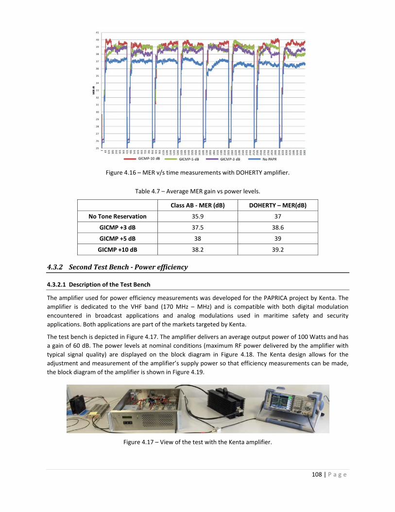
108 | P a g e
Figure 4.16 – MER v/s time measurements with DOHERTY amplifier.
Table 4.7 – Average MER gain vs power levels.
Class AB ‐ MER (dB) DOHERTY – MER(dB)
No Tone Reservation 35.9 37
GICMP +3 dB 37.5 38.6
GICMP +5 dB 38 39
GICMP +10 dB 38.2 39.2
4.3.2 SecondTestBench‐Powerefficiency
4.3.2.1 Description of the Test Bench
The amplifier used for power efficiency measurements was developed for the PAPRICA project by Kenta. The
amplifier is dedicated to the VHF band (170 MHz – MHz) and is compatible with both digital modulation
encountered in broadcast applications and analog modulations used in maritime safety and security
applications. Both applications are part of the markets targeted by Kenta.
The test bench is depicted in Figure 4.17. The amplifier delivers an average output power of 100 Watts and has
a gain of 60 dB. The power levels at nominal conditions (maximum RF power delivered by the amplifier with
typical signal quality) are displayed on the block diagram in Figure 4.18. The Kenta design allows for the
adjustment and measurement of the amplifier’s supply power so that efficiency measurements can be made,
the block diagram of the amplifier is shown in Figure 4.19.
Figure 4.17 – View of the test with the Kenta amplifier.
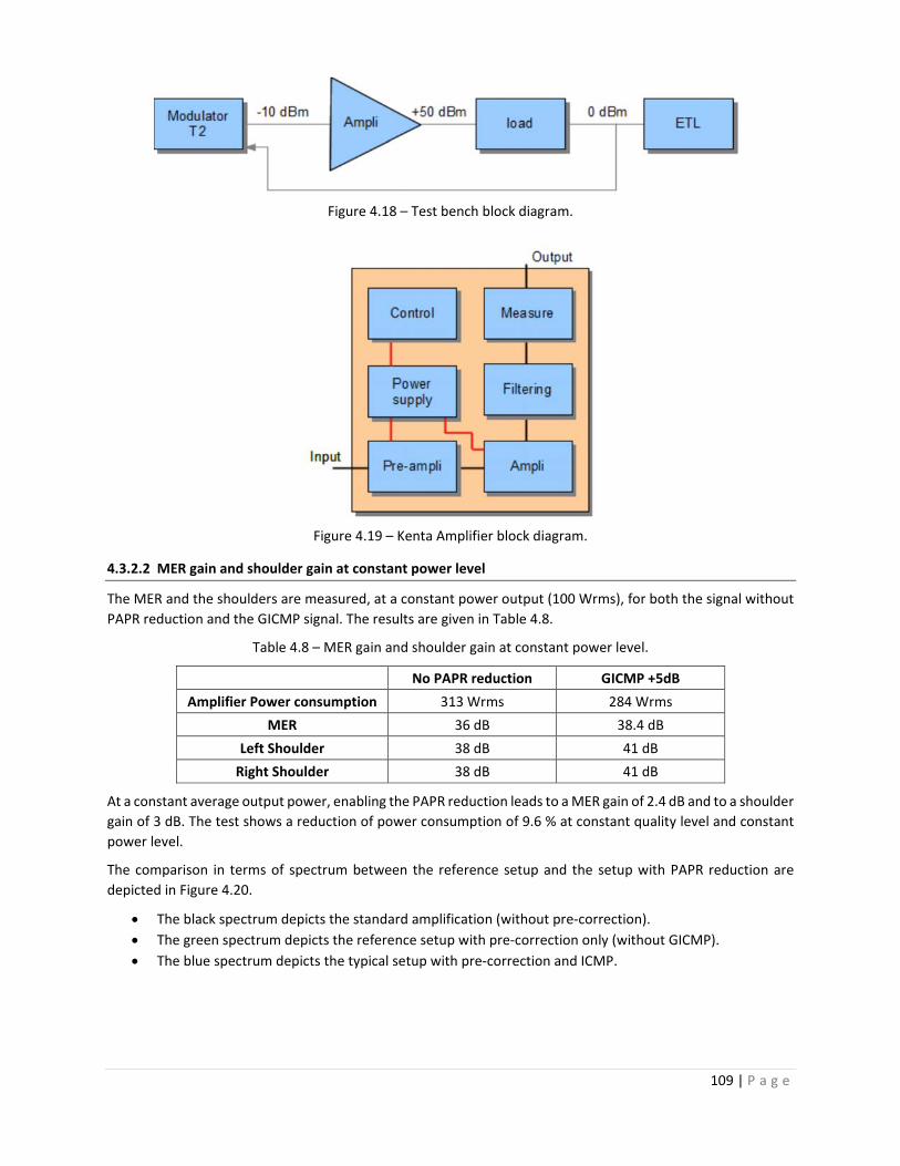
109 | P a g e
Figure 4.18 – Test bench block diagram.
Figure 4.19 – Kenta Amplifier block diagram.
4.3.2.2 MER gain and shoulder gain at constant power level
The MER and the shoulders are measured, at a constant power output (100 Wrms), for both the signal without
PAPR reduction and the GICMP signal. The results are given in Table 4.8.
Table 4.8 – MER gain and shoulder gain at constant power level.
No PAPR reduction GICMP +5dB
Amplifier Power consumption 313 Wrms 284 Wrms
MER 36 dB 38.4 dB
Left Shoulder 38 dB 41 dB
Right Shoulder 38 dB 41 dB
At a constant average output power, enabling the PAPR reduction leads to a MER gain of 2.4 dB and to a shoulder
gain of 3 dB. The test shows a reduction of power consumption of 9.6 % at constant quality level and constant
power level.
The comparison in terms of spectrum between the reference setup and the setup with PAPR reduction are
depicted in Figure 4.20.
The black spectrum depicts the standard amplification (without pre‐correction).
The green spectrum depicts the reference setup with pre‐correction only (without GICMP).
The blue spectrum depicts the typical setup with pre‐correction and ICMP.
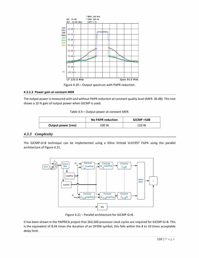
110 | P a g e
Figure 4.20 – Output spectrum with PAPR reduction.
4.3.2.3 Power gain at constant MER
The output power is measured with and without PAPR reduction at constant quality level (MER: 36 dB). This test
shows a 10 % gain of output power when GICMP is used.
Table 4.9 – Output power at constant MER.
No PAPR reduction GICMP +5dB
Output power (rms) 100 W 110 W
4.3.3 Complexity
The GICMP‐G=8 technique can be implemented using a Xilinx Virtex6 VLX195T FGPA using the parallel
architecture of Figure 4.21.
Figure 4.21 – Parallel architecture for GICMP‐G=8.
It has been shown in the PAPRICA project that 263,560 processor clock cycles are required for GICMP‐G=8. This
is the equivalent of 8.04 times the duration of an OFDM symbol, this falls within the 8 to 10 times acceptable
delay limit.

111 | P a g e
4.4 Conclusion
As studied in this chapter, the proposed GICMP technique yields a MER gain of up to 2.3 dB when used with a
class AB and DOHERTY amplifier (the two most common types of amplifiers). It was further shown that selecting
a power constraint level of +5 dB instead of the +10 dB as allowed by the DVB‐T2 standard is a good tradeoff
since it has a minimal impact on the output signal power while keeping a MER gain of 2 dB. All these
measurement results were obtained from the experimental platform developed by the engineers of TeamCast
and fed with the IQ samples provided by means of a dedicated software simulator.
The selected GICMP technique was also tested with a power amplifier developed by Kenta, the GICMP yields a
MER gain of 2.4 dB. The benefits of the GICMP technique can either:
be turned into a gain of output power at constant MER: with the same design and the same power
supply settings, the power amplifier is able to deliver 10 % more power thanks to the PAPR reduction
mechanism, or
be turned into a reduction of energy consumption at constant output power and constant MER: with
the same output power and the same target MER, the proposed PAPR reduction is able to reduce the
energy consumption by 10%.
This means that a transmitter with a basic efficiency of 40 % can have its efficiency boosted to about 44%, only
by applying the GICMP PAPR reduction process.
A second series of tests using an optimized power amplifier featuring adjustments and measurements showed:
a quality gain of up to +2.4 dB with reduced mean signal level increase, at constant output power level
and constant system setup,
that this quality gain can be turned to an output power handling increase of +10 %, at constant quality
level (36 dB MER) and constant system setup,
that this quality gain can be turned to a reduction of the energy consumption of ‐10 %, at constant
quality level (36 dB MER) and constant output power level, with a slight change in the system setup.
This final result confirms the “green” benefit of the proposed algorithm at a time when all transmitter
manufacturers are working at improving the energy efficiency of their systems.


113 | P a g e
Joint Channel Estimation
and PAPR Reduction Scheme
5.1 Introduction
The TR technique adopted in DVB‐T2 requires the reservation of almost one percent of the available subcarriers
for PAPR reduction. DVB‐T2 also allocates pilots for channel estimation purposes (refer to paragraph 1.3.6).
Researchers [149] [150] [151] [152] have proposed to combine both Channel Estimation and PAPR Reduction
techniques in such a way to reduce the total number of reserved subcarriers, hence enhancing spectral
efficiency.
In [149], a watermark sequence is overlaid, in time domain, to the OFDM signal to allow for a joint channel
estimation and PAPR reduction. Through an iterative process, the watermark sequence providing the lowest
PAPR is selected among a set of Kasami sequences, which are known by the receiver. The main disadvantage of
this technique, is that the receiver must apply a trial and error mechanism in order to determine the watermark
used in order to perform channel estimation. In [150], all pilots, including those reserved for channel estimation,
are removed. Instead, a Generalized Chirp‐Like (GCL) sequence is superimposed to the data symbols in order to
allow for a joint channel estimation and PAPR reduction. Even though the method proposed in [150] is
interesting, it is limited by the maximum power allowed to the pilots versus the power allocated to data
subcarriers. The combination of Partial Transmit Sequence (PTS) and channel estimation have been proposed in
[151] and [152]. These techniques inherit the large resource requirements, in terms of memory and
computations, of PTS.
This chapter takes the Channel Estimation and PAPR Reduction (CEPR) technique [153] [154] [155] as a base to
propose new joint channel estimation techniques that are both performant and simple to implement. The CEPR
requires the reserved pilot values to be related to one another by a multiplicative geometric relationship. At the
transmitter, CEPR uses an exhaustive search algorithm to determine the best sequence in terms of PAPR
reduction. At the receiver, the transmitted pilot values are obtained by applying a blind detection algorithm
before performing channel estimation.
This chapter starts by introducing the CEPR technique. Then various enhancements are proposed, the first avoids
the use of costly exhaustive search but reduces only one signal peak, the second and third rely on shifting and
interleaving of multiple pilot sequences in order to both avoid exhaustive search and reduce multiples signal
peaks.

114 | P a g e
5.2 Definitions
The CEPR technique requires the reserved pilots to respect a geometric relationship. A new annotation,
compared to the previous chapters, is presented in this section in order to better define the relationship
between the reserved subcarriers.
Let be the set of the pilot positions reserved for joint channel estimation and PAPR reduction:
, … ,
and let be the set of pilot values transmitted over these positions:
, … ,
To associate a pilot value with its corresponding position , a bijective function f over the integer field is
defined as follows:
↦ f: → ∈ , 0 1
Then, the modulated subcarriers … of the OFDM symbol in the frequency domain can be
expressed as:
∈
where and represent the pilot subcarriers and the data subcarriers respectively.
For the sake of clarity and to demonstrate the need for the function , we consider the simple example with5, 2, 1 0 and 3 1, then
1, 3
and is then given by:
, , , ,
Therefore, the transmitted time domain signal is given by:
where , and are the time domain representation of | ,…., , | ,…., and | ,…., respectively.
The values of must be chosen in such a way to reduce the PAPR of .
5.3 CEPRTechnique
5.3.1 Sequencedesign
The Channel Estimation and PAPR reduction (CEPR) technique [153] [154] [155] uses some of the scattered pilots
dedicated to channel estimation for both channel estimation and PAPR reduction purposes. The main advantage
of CEPR compared to the conventional TR method is a gain in spectral efficiency.
A CEPR pilot sequence is built based on a multiplicative law between the reserved pilots:
∀ ∈ 0, … , 2 with (5.1)
or equivalently
∀ ∈ 0, … , 1 (5.2)

115 | P a g e
The multiplicative relationship is depicted in Figure 4.1 and has three parameters:
: the boost factor, ∈ R
: the initial phase or the phase correction, ∈ 0,2π
: the phase increment, ∈ 0,2π
Figure 5.1 – Multiplicative law scheme.
5.3.2 PAPRreduction
Similar to PTS and Selective Mapping (SLM), CEPR uses an exhaustive search algorithm to determine the best
parameter values (for , and ) that yield the best PAPR reduction [153].
To limit the number of candidates:
is set to a predefined value known at the receiver,
and are chosen from predefined sets of discrete values with discrete steps and
respectively.
The values of and determine the algorithm complexity: the smaller these steps are the more
candidates have to be tested and the higher the number of required operations (refer to paragraph 5.3.6 for
more details). They also determine the accuracy of the channel estimation as presented in the next paragraph.
5.3.3 PilotsRecovery
In a conventional channel estimation scheme, where the channel estimation pilot values are known at the
receiver, and under the following assumptions: (1) frequency nonselective fading per subcarrier, (2) time
invariance during one OFDM symbol and (3) GI long enough to mitigate any ISI and ICI, the received pilots of
symbol at the output of the FFT are given by:
. where
represents the vector of received values at the pilot positions,
represents the channel response matrix relative to the pilot positions ( is a diagonal matrix),
represents the vector of transmitted pilots, and
represents the vector of AWGN noise.
: variable in discrete domain
: variable in discrete domain
C0
C2
C1: fixed value
C0= ejCk= ej(+k)

116 | P a g e
The transmitted pilot vector being known at the receiver, an estimation of the channel response is computed
as follows:
Or equivalently (since is diagonal),
Where , , are the estimated channel frequency response, the received symbol and the transmitted
symbol for the subcarrier of the OFDM symbol respectively.
An estimation of the channel response is then obtained by filtering the obtained coefficients of by
coefficients using some conventional interpolation filters such as the Wiener filter. This conventional channel
estimation process is shown in Figure 5.2.
Figure 5.2 – Conventional channel estimation scheme.
However, in CEPR, the pilot values that yield the best PAPR reduction are chosen at the transmitter and are
not known at the receiver. To circumvent this problem at the receiver, CEPR uses the geometric relationship
between the pilot values to generate an estimation of the transmitted pilots before performing channel
estimation. This process is called blind detection [153] and is described in the remainder of this paragraph.
The channel coefficients are assumed to be almost constant over two successive OFDM symbols [153], i.e.:
Then an initial estimated version of can be obtained as follows:
.
and for each pilot:

117 | P a g e
An enhanced estimation can be produced by exploiting the relationship between consecutive pilots.
where
∗
where | denotes the decision function of in discrete domain with a step .
The estimation of and enable the computation of the estimated transmitted pilot sequence which is then
used to estimate the channel frequency response for the pilot pilot using the following relation:
The above process can be achieved iteratively to improve the estimation of the pilot sequences and the channel
coefficients. The estimation process is depicted in Figure 5.3, the differences with the conventional scheme are
being highlighted red. The CEPR requires the storage in memory of the frequency response of the previous
symbol , which is then used along with the received pilot to compute an estimation of the transmitted
pilot . The channel response of the current symbol is then computed using and .
Figure 5.3 – Blind channel estimation scheme.
5.3.4 Blockdiagram
The CEPR principle is summarized in the block diagram in Figure 5.5. Function symbolizes the geometric
relationship between the reserved pilots and () symbolizes the inverse operation performed at the receiver
in order to recover the transmitted pilots.

118 | P a g e
Figure 5.4 – CEPR block diagram.
5.3.5 ErrorDetectionProbabilityofCEPR
The target of this section is to analytically evaluate the Error Detection Probability (EDP) of a CEPR sequence
assuming an AWGN channel. The EDP performance is important to assess the impact of the blind detection
algorithm on channel estimation.
It has been shown in [153] that for CEPR the received pilot can be expressed as:
PpneC ppj
p )(
where is the value of the AWGN of zero mean and varianceσ .
According to [153] , the EDP of and are given by:
18
(5.3)
1√ λ2σ
(5.4)
Looking at equations (5.3) and (5.4) it can be seen that increasing and translates into better EDP
performance.
5.3.6 Complexity
For each OFDM symbol, the total number of possible combinations tested by CEPR is given by:
2
2 (5.5)
The exhaustive search algorithm consists of the following steps:
Generate pilot sequences.
Transform each sequence to the time domain and add it to the useful signal.
Compute and store the PAPR value along with the corresponding values of and .

119 | P a g e
Once all combinations are tested, the values of and corresponding to the lowest PAPR are retained
and used to generate the optimized pilot sequence.
Table 5.1 ‐ Number of operations required to test one candidate by CEPR.
Operations Remarks
Compute IFFTs 4 log – 6 8 Using split‐radix algorithm
Add to original signal 2 For each sample 2 additions
(1 for the real part and 1 for the imaginary part)
Finding the maximum 4 For each sample 2 multiplications, 1 addition and
1 subtraction
Generating the pilots 82 For each pilot 1 cosine, 1 sine and 2
multiplications
Adding to 2 For each sample 2 additions
(1 for the real part and 1 for the imaginary part)
The number of operations required by the CEPR algorithm to test one candidate is summarized in Table 5.1.
Floating operations are counted as 1 operation and trigonometric functions are accounted for as 40 operations.
The algorithm runs in . . The total number of operations required by CEPR per OFDM symbol is given
by:
4 2 81 8 (5.6)
The impact of the step sizes can be seen by analyzing equation (5.6) and (5.5). The smaller and , the
larger the number of candidates being tested by the algorithm. The increased number of candidates increases
the chances of finding a better sequence in terms of PAPR reduction, however it considerably increases the
complexity (especially that each candidate requires the computation of an IFFT) and also reduces the EDP
performance as explained in paragraph 5.3.5.
5.4 FastCEPRTechnique
5.4.1 SequenceDesign
The main drawback of CEPR dwells in the exhaustive search for the best pilot sequence at the transmitter
performed for each OFDM symbol. The aim of the Fast CEPR (F‐CEPR) method is to reduce the complexity of the
search algorithm while keeping the channel estimation capabilities.
In contrast to CEPR, which allocates non‐uniformly distributed pilots, F‐CEPR uses a set of uniformly allocated
pilots. The set of pilot positions for an F‐CEPR sequence is given by:
, 0
In this study we consider the 2K mode, where the number of subcarrier is =2048. For practical reasons, the
number of reserved subcarriers is considered to be a divider of ( =32, 64, 128, 256). As in CEPR, the pilot
values , … , are related to each other through the same multiplicative law of equation (5.1).
The time domain representation of is given by:
1
√. (5.7)

120 | P a g e
If is selected to be multiple of
.2
, 0 (5.8)
Then
λM
√ 0
0 (5.9)
The details are provided in Annex B. The amplitude and phase of the time‐domain pilot signal are then given by:
| | λM
√ 0
0 (5.10)
(5.11)
All the non‐zero values of have an amplitude equal to √
and are referred to as peaks. Let Υ be the set of
peak positions of :
Υ , 0 0 (5.12)
The time domain signal has the following properties
Property 1: The number of peaks of | | is given by:
|Υ|
Property 2: The peak positions are periodic with a period equal to .
Property 3: The position of the peak is given by:
5.4.2 PAPRReduction
The relation between the position of the peak and can be obtained by combining Property 3 and equation
(5.8). It is given by:
∆2
(5.13)
Same as CEPR takes values from a predefined set of discrete values
.
If is chosen to be a multiple of , then will also be a multiple of and the condition of (5.8) will be
verified. In this case (5.13) becomes:

121 | P a g e
2
And the position of the first peak of is given by:
12
(5.14)
It can be seen from (5.14) that the position of the first peak of can be controlled by the value of .
Figure 5.5 shows the layout of F‐CEPR sequence in time domain for different values of . Increasing M decreases
the number of peaks (see Property 1).
Figure 5.6 shows the impact of changing on the peak positions of the F‐CEPR sequence in time domain. It is
clear that the location of the peaks can be controlled by adjusting the value of .
Figure 5.5 – F‐CEPR sequence in time domain for =256 and =16, 32, 64.
Figure 5.6 – F‐CEPR sequence in time domain for =256, =32 and different values of .

122 | P a g e
5.4.2.1 Peak Detection
F‐CEPR starts by searching for the highest peak of the OFDM symbol in time domain. This operations requires
traversing all the samples of the OFDM symbol. Let represent the position of the highest signal peak of
and let represents its value.
| | | |
5.4.2.2 Computation of
The idea of F‐CEPR is to choose in such a way that the position of the first peak of coincides with the position
of the detected peak of .
1
Then using (5.13),
2
2.1
And
2. (5.15)
5.4.2.3 Computation of
Now that the first peak position of coincides with the detected peak at position , F‐CEPR computes the
correction phase in such a way to reduce the phase gap between and .
Same as CEPR, is chosen from a discrete set of values with a step
(5.16)
where | denotes the decision function of in discrete domain with a step .
5.4.2.4 Boost Factor
The boost factor is chosen according to the targeted reduction value. The value of is agreed upon between
the transmitter and the receiver via signaling before data transmission starts.
5.4.2.5 Pilot generation
After computing according to (5.15) and according to (5.16), F‐CEPR generates the pilot sequence
according to (5.9) and adds it the useful signal . This process will be referred to as the “reduction of one signal
peak” and is depicted in Figure 5.7.

123 | P a g e
Figure 5.7 – F‐CEPR pilot sequence generation algorithm.
5.4.3 Complexity
The number of operations required by the F‐CEPR algorithm to reduce one peak of an OFDM symbol is detailed
in Table 5.2
Table 5.2 ‐ Number of operations required by F‐CEPR
Operations Remarks
Finding the maximum 4 Iterate over all subcarriers
Computing 3 According to eq. (5.15)
Computing 44 According to eq. (5.16), requires one tangent
Generating the pilots 81 According to eq. (5.9)
Adding to 2
The total number of operations is given by:
6 82 47 (5.17)
CEPR runs in . whereas F‐CEPR run in . Moreover the constant term in the expression
of , in equation (5.6) adds a considerable computational burden. The latter shows that decreasing the
discrete step (and equivalently by a factor of 2 increases the number of operations required for
CEPR by a factor of 4, while for F‐CEPR, it slightly increases with the increment of .

124 | P a g e
Table 5.3 – Comparison between the numbers of operations required for CEPR and F‐CEPR
2048 32 16 16 9.91E+07 1.50E+04
2048 32 32 32 3.97E+08 1.50E+04
2048 64 16 16 1.02E+08 1.76E+04
2018 64 32 32 4.07E+08 1.76E+04
5.5 FastShiftedCEPRTechnique
The F‐CEPR technique is designed to reduce exactly one peak. Better PAPR reduction can be achieved if more
peaks can be reduced. The Fast Shifted (FS‐CEPR) method consists of using multiple superimposed and shifted
F‐CEPR sequences (different pilot sequences are overlaid on each other) to create a final pilot stream.
5.5.1 SequenceDesign
The Shifting Order, , refers to the additional number of peaks that FS‐CEPR can reduce:
For 0, the FS‐CEPR is equivalent to F‐CEPR
For , the FS‐CEPR reduces additional peaks for a total of 1 reduced peaks.
The Shifting Step, , represents the number of positions used to shift each F‐CEPR sequence in frequency
domain from the previous one.
A typical layout of FS‐CEPR is described in Figure 5.8. The FS‐CEPR sequence has the following properties:
An FS‐CEPR sequence consists of 1 F‐CEPR sub‐sequences.
The number of pilots in a F‐CEPR sub‐sequence is given by:
1 . (5.18)
The set of pilot positions belonging to the F‐CEPR sub‐sequence is given by:
∈ , . .
The F‐CEPR sub‐sequence is given by
, ∈0
(5.19)
Every two sub‐sequences have all their chips superimposed except chips as shown in Figure 5.8.. The
shifting provides the receiver with additional information that can be exploited to perform the blind
channel estimation.
The FS‐CEPR sequence can be defined as follows:
,

125 | P a g e
Figure 5.8 – Fast Shifted CEPR with 2 and 2.
5.5.2 PAPRReduction
The parameters ( , and ) of each F‐CEPR sub‐sequence are calculated using the F‐CEPR algorithm
described in paragraph 5.4.2. The flowchart for FS‐CEPR is shown in Figure 5.9. In the flowchart, , represent
the time domain version of the , definer in (5.19) and represent the current iteration number.
Figure 5.9 – FS‐CEPR flowchart.

126 | P a g e
5.5.3 PilotRecoverywithFS‐CEPR
Similar to CEPR, the pilots must be recovered through blind detection at the receiver in order to perform channel
estimation. The FS‐CEPR sequence can be reconstructed by estimation of the and values for each F‐CEPR
sub‐sequence. This can be performed using a modified version of the scheme described in paragraph 5.3.3 which
takes advantage of the shifting between consecutive sequences. The process is illustrated and explained in Table
5.4.
Table 5.4 – FS‐CEPR blind detection.
Layout Explanation
For 0 2 only chips from , are present: ,
, can be estimated from , using the same
algorithm as CEPR.
For 2 4 only chips from , and ,
are present: , ,
The previously computed , values can be
subtracted from , to obtain:
, ,
, can be estimated from using the same
algorithm as CEPR.
For 4 6 only chips from , , ,
and , are present: , , ,
The previously computed , and , values
can be subtracted from , to obtain:
, , ,
, can be estimated from using the same
algorithm as CEPR.
In the general case, the estimate of the transmitted pilots can be obtained from the received pilots by applying the following algorithm.
Initialisation: Set 1
Step 1: Increment and determine the set of useful pilots , for sequence by applying:
,
, 0
, , 0 1 SS
Step 2: Calculate and by applying the same algorithm as F‐CEPR to , .
Step 3: Compute and store , :
, ∈
0 (5.20)
Step 4: Go to Step 1 and repeat while

127 | P a g e
At the completion of the algorithm, the estimated pilots are given by:
, (5.21)
The estimated pilot values can then be used to perform channel estimation.
5.5.4 ErrorDetectionProbabilityofFS‐CEPR
Following the same methodology as in [154], the received chip of the transmitted superimposed
sequence can be written in the general case as:
, , , , (5.22)
where ∑ , can be referred as Inter‐Sequence Interference (ISI), and
, is the AWGN value at the chip of the sequence of zero mean and variance equal to σ .
For 0 and0 , there is no ISI. Then, we can write
, , , 0
Using equation (A.16) of [154] the probability of error on is given by:
∆ ⟶ 0,1
21
and from (A.27) of [154], the probability of error on becomes:
⟶ 0,2
For 1, the first sequence , interferes with , . Then, the received sequence is deduced from (5.22) as:
, , , ,
Assuming small angles approximation on and :
∆ ⟶ 0,21
41
and
⟶ 0,2
2
In the general case, it can be shown that the probability of error on and are given by:
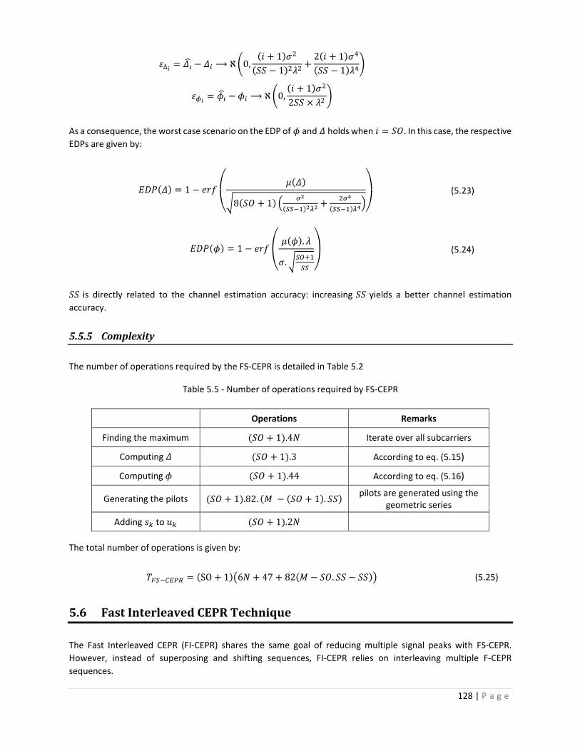
128 | P a g e
∆ ⟶ 0,11
2 11
⟶ 0,1
2
As a consequence, the worst case scenario on the EDP of and holds when . In this case, the respective
EDPs are given by:
18 1
(5.23)
1.
. (5.24)
is directly related to the channel estimation accuracy: increasing yields a better channel estimation
accuracy.
5.5.5 Complexity
The number of operations required by the FS‐CEPR is detailed in Table 5.2
Table 5.5 ‐ Number of operations required by FS‐CEPR
Operations Remarks
Finding the maximum 1 .4 Iterate over all subcarriers
Computing 1 .3 According to eq. (5.15)
Computing 1 .44 According to eq. (5.16)
Generating the pilots 1 .82. 1 . pilots are generated using the
geometric series
Adding to 1 .2
The total number of operations is given by:
SO 1 6 47 82 . (5.25)
5.6 FastInterleavedCEPRTechnique
The Fast Interleaved CEPR (FI‐CEPR) shares the same goal of reducing multiple signal peaks with FS‐CEPR.
However, instead of superposing and shifting sequences, FI‐CEPR relies on interleaving multiple F‐CEPR
sequences.

129 | P a g e
5.6.1 Sequencesdesign
In FI‐CEPR, the set of pilots originally assigned for PAPR reduction is distributed among (Interleaving
Order) sequences.
Figure 5.10 displays a typical layout for different values of . For 1, FI‐CEPR is equivalent to F‐CEPR.
Figure 5.10 –Fast Interleaved CEPR for M=16 and different values of IO
The FS‐CEPR sequence has the following properties:
An FS‐CEPR sequence consists of F‐CEPR sub‐sequences.
The number of pilots in each F‐CEPR sub‐sequence is given by:
(5.26)
The set of pilot positions belonging to the F‐CEPR sub‐sequence is given by:
. 1, 1
The F‐CEPR sub‐sequence is given by:
, ∈0e
(5.27)
The FI‐CEPR sequence can be defined as follows:
,
For practical reasons is chosen to be equal to a power of two.

130 | P a g e
5.6.2 PAPRreduction
For each sequence, , and are calculated using the same algorithm, described in section 0, as the F‐CEPR
method. Fast Interleaved CEPR (FI‐CEPR) allows for the reduction of multiple signal peaks. FI‐CEPR overcomes
the limitation of F‐CEPR which reduces only one signal peak. The flowchart for FI‐CEPR is shown in Figure 5.11.
In the flowchart, , represent the time domain version of the , definer in (5.27) and represent the
current iteration number.
Figure 5.11 – FI‐CEPR flowchart.
5.6.3 Pilotrecoveryandchannelestimation
The estimation , of each sub‐sequence can be retrieved from the received sub‐sequence , using the same
blind detection algorithm as CEPR. The only difference exists in the length of interleaved sequences.
, ,
The reconstructed FI‐CEPR sequence can then be used for channel estimation purposes.
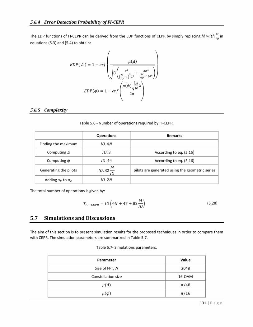
131 | P a g e
5.6.4 ErrorDetectionProbabilityofFI‐CEPR
The EDP functions of FI‐CEPR can be derived from the EDP functions of CEPR by simply replacing in
equations (5.3) and (5.4) to obtain:
1
8
1λ
2σ
5.6.5 Complexity
Table 5.6 ‐ Number of operations required by FI‐CEPR.
Operations Remarks
Finding the maximum . 4
Computing . 3 According to eq. (5.15)
Computing . 44 According to eq. (5.16)
Generating the pilots . 82 pilots are generated using the geometric series
Adding to . 2
The total number of operations is given by:
6 47 82 (5.28)
5.7 SimulationsandDiscussions
The aim of this section is to present simulation results for the proposed techniques in order to compare them
with CEPR. The simulation parameters are summarized in Table 5.7.
Table 5.7‐ Simulations parameters.
Parameter Value
Size of FFT, 2048
Constellation size 16‐QAM
/48
/16

132 | P a g e
5.7.1 PAPREffectiveGain
The PAPR effective gain metric was introduced in [154] to measure the performance of the CEPR technique. It
quantifies the difference between the PAPR gain ∆ and the power increase ∆ induced by the pilot sequences
(see Figure 5.12).
∆ ∆
The PAPR of any signal can be reduced by either reducing the amplitude of its maximum (reducing the numerator
of the PAPR formula) or by increasing its average power (increasing the denominator of the PAPR formula). In
this study all power constraints imposed on the reserved subcarriers have been lifted, this is why the PAPR
effective gain is used in this section since it reflects only the amount of PAPR reduction originating for signal
peak reduction. Moreover, the PAPR effective gain metric allows for the measurement the performance of the
proposed techniques against those of CEPR.
Figure 5.12 – PAPR effective gain.
5.7.2 F‐CEPRPerformance
In Figure 5.13, the performance of F‐CEPR in terms of effective PAPR gain is presented as a function of the boost
factor, , for different values of . The PAPR effective gain of CEPR from [154] is also plotted as a reference.
The PAPR effective gain increases with . Also, for a fixed value of , the best value of is different.
Figure 5.13 – PAPR effective gain as a function of for F‐CEPR, =2048.

133 | P a g e
The best values for are summarized in Table 5.8. In all cases the PAPR effective gain of F‐CEPR varies between
0.5 dB and 0.7 dB which translates into a gap of 0.5 to 0.7 dB compared to CEPR. This can be explained by the
fact that F‐CEPR performs only one iteration and reduces only one signal peak compared to CEPR which performs
an exhaustive search algorithm in order to find the best sequence.
Table 5.8 – Best values of for various configurations.
Technique (dB) PAPR Effective Gain (dB)
F‐CEPR M=16 12 0.61
F‐CEPR M=64 8 0.64
F‐CEPR M=128 4 0.79
CEPR /16 2 1.23
CEPR /32 2 1.43
5.7.3 ImpactofthediscretestepsonEDPperformance
The EDP curves for the two CEPR configurations considered from [154] are plotted in Figure 5.14 and Figure
5.15. For both and , the EDP performance is better for larger steps.
However the PAPR gain is better for smaller steps (i.e. 1.23 dB for /16 and 1.43 dB for /32, see Table 5.8). For smaller steps more candidates are tested by the exhaustive search algorithm, hence the chances to find
better sequences are higher.
Figure 5.14 – for CEPR.
Figure 5.15 – for variable values of .
The step size is also an important factor in defining the complexity of the CEPR algorithm (see equations (5.5)
and (5.6)). Table 5.9 displays side by side the PAPR gain, EDP performance and number of operations required.
CEPR with a step of /16 have a better performance complexity tradeoff compared to CEPR with a step of /32 and is chosen as a base line for comparison in the coming paragraphs.
Table 5.9 – EDP and Effective PAPR gain for CEPR.
Effective PAPR
Gain (dB) SNR for 10‐3
(dB) SNR for 10‐3
(dB)
/16 1.23 2.9 3.6 8.42E+07
/32 1.43 4.4 6.6 3.37E+08

134 | P a g e
5.7.4 ImpactofMand onEDPPerformance
The EDP functions of and are drawn in Figure 5.16 and Figure 5.17 for various values of . The EDP graphs
are obtained by varying the SNR at the receiver. The EDP performance is assessed by looking at the SNR required
to maintain an EDP of 10‐3 (the lower the SNR required, the better). It can be noticed that the EDP performance
increases with . In fact for larger values of , more samples are presented to the blind detection algorithm.
The information carried by the extra samples is used to generate a better estimation hence the better EDP
performance.
Figure 5.16 – for various values of .
Figure 5.17 – for various values of .
In Figure 5.18 and Figure 5.19, the EDP functions of and are drawn for =64 and for variable values of . The higher the value, the more the pilots are boosted and the more they are resilient to noise at the receiver.
This explains why for both the EDP functions the performance increases with .
Figure 5.18 – for various values of . Figure 5.19 – for various values of .
By comparing the previous charts, it can be seen that has a bigger impact on EDP performance than .
Increasing from 16 to 32 translates into 1.65 dB of SNR gain at EDP 10‐3. Whereas increasing by 1 dB yields
an SNR gain of 0.5 dB.
In the remainder of this section the F‐CEPR configuration with =64 and =8 dB is chosen as a base line for
comparison:

135 | P a g e
With =64, 3.125% (64 out of 2048) of the OFDM subcarriers are used for joint PAPR and channel
estimation (compared to 6.25% with M=128). This configuration reduces the channel estimation
overhead in DVB‐like systems where typically 8.33% (1 out of each 12 subcarriers) of subcarriers are
allocated for channel estimation alone.
With =8 dB, the power allocated to the pilots falls within the acceptable range (less than 10 dB allowed)
by the DVB‐T2 standard
The PAPR gain is only 0.14 dB lower than with =128.
5.7.5 FS‐CEPRPerformance
Figure 5.20 shows the performance of FS‐CEPR in terms of PAPR effective gain. It is clear that FS‐CEPR always
outperforms F‐CEPR by an amount varying between 0.3 dB (for =16 and =14 dB) and 0.46 dB (for =128 and
=10 dB). Moreover, compared with the CEPR technique, the FS‐CEPR method reduces the gap to 0.12 dB
(compared to 0.59 dB for F‐CEPR). The increase in performance is due to the additional number of peaks reduced
by FS‐CEPR (i.e. for =3 FS‐CEPR targets 2 additional peaks compared to F‐CEPR).
FS‐CEPR with =64 and =10 dB is selected as offering a good compromise between PAPR reduction, number
of subcarriers reserved and boost factor.
Figure 5.20 – PAPR effective gain as a function of for FS‐CEPR, =3, =10.
5.7.6 FI‐CEPRPerformance
The effective PAPR gain of FI‐CEPR is shown in Figure 5.21. FI‐CEPR outperforms F‐CEPR by 0.06 dB (for =32
and =16), 0.15 dB (for =64 and =14) and by 0.22 dB (for =127 and =12). FI‐CEPR with =8 targets and
reduces 8 signal peaks. However it does not exhibit the same PAPR gain as FS‐CEPR with SO=3 which only targets
3 peaks.
This can be explained by looking at the length of the used subsequences. For FI‐CEPR with =8, each
subsequence has a length of 6 (see equation (5.18)). However, for FS‐CEPR with =3 and =10, each
subsequence has a length of 24 (see equation (5.26)). The larger the subsequence, the more concentrated the
power is in time domain, the finest the PAPR reduction which explains the difference in performance.
FI‐CEPR with =64 and =10 dB is selected as offering a good compromise between PAPR reduction, number
of reserved subcarriers and boost factor.
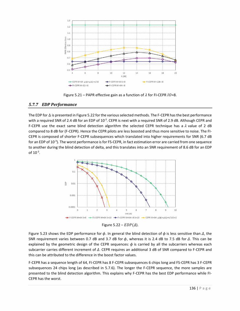
136 | P a g e
Figure 5.21 – PAPR effective gain as a function of for FI‐CEPR =8.
5.7.7 EDPPerformance
The EDP for ∆ is presented in Figure 5.22 for the various selected methods. The F‐CEPR has the best performance
with a required SNR of 2.4 dB for an EDP of 10‐3. CEPR is next with a required SNR of 2.9 dB. Although CEPR and
F‐CEPR use the exact same blind detection algorithm the selected CEPR technique has a value of 2 dB
compared to 8 dB for (F‐CEPR). Hence the CEPR pilots are less boosted and thus more sensitive to noise. The FI‐
CEPR is composed of shorter F‐CEPR subsequences which translated into higher requirements for SNR (6.7 dB
for an EDP of 10‐3). The worst performance is for FS‐CEPR, in fact estimation error are carried from one sequence
to another during the blind detection of delta, and this translates into an SNR requirement of 8.6 dB for an EDP
of 10‐3.
Figure 5.22 – ).
Figure 5.23 shows the EDP performance for . In general the blind detection of is less sensitive than , the
SNR requirement varies between 0.7 dB and 3.7 dB for , whereas it is 2.4 dB to 7.5 dB for . This can be
explained by the geometric design of the CEPR sequences: is carried by all the subcarriers whereas each
subcarrier carries different increment of . CEPR requires an additional 3 dB of SNR compared to F‐CEPR and
this can be attributed to the difference in the boost factor values.
F‐CEPR has a sequence length of 64, FI‐CEPR has 8 F‐CEPR subsequences 6 chips long and FS‐CEPR has 3 F‐CEPR
subsequences 24 chips long (as described in 5.7.6). The longer the F‐CEPR sequence, the more samples are
presented to the blind detection algorithm. This explains why F‐CEPR has the best EDP performance while FI‐
CEPR has the worst.

137 | P a g e
Figure 5.23 – ).
5.7.8 Comparison
Table 5.10 displays a comparison between the various selected techniques and CEPR. It can be seen that all
techniques require significantly less operations (1000 less) compared to CEPR which is based on an exhaustive
search algorithm. The FI‐CEPR and FS‐CEPR bridge the PAPR gain gap between F‐CEPR and CEPR. The
improvement in PAPR reduction comes at a small cost in SNR requirements. However all techniques fall within
the 10 dB range required by DVB like systems.
Table 5.10 – Comparison table.
Technique
(dB) PAPR Effective
Gain (dB) SNR at )
10‐3 (dB) SNR at
10‐3 (dB) Operations
CEPR 64 2 1.23 3.70 5.30 1.02E+08
F‐CEPR 64 8 0.65 0.75 2.50 1.76E+04
FI‐CEPR = 8 64 10 0.73 4.20 6.60 5.72E+04
FS‐CEPR =3‐ =10 64 10 1.04 3.69 9.15 1.04E+05
5.8 Conclusion
This chapter presented the CEPR technique which allows for joint PAPR reduction and channel estimation to be
performed using the same set of reserved pilots. The reserved pilots are chosen to be elements of a geometric
series in order to allow channel estimation by blind detection to be performed at the receiver. In order to find
the best sequence respecting the geometric relationship and yielding PAPR reduction, CEPR uses an exhaustive
search algorithm similar to PTS and SLM. This renders CEPR computationally demanding.
The peak position, amplitude and phase of the time domain version of uniformly distributed reserved pilots can
be controlled using only three parameters. F‐CEPR computes these parameters in order to reduce one signal
peak thus avoiding the use of any exhaustive search.
The PAPR gain can be increased by targeting and reducing more signal peaks. FI‐CEPR and FS‐CEPR target more
signal peaks, the first by interleaving multiple F‐CEPR sequences and the second by shifting and superposing
multiple F‐CEPR sequences. The interleaving and superposing is required to keep enough information on each
sub‐sequence for the receiver to perform blind detection. All the proposed techniques are significantly less
complex than the CEPR technique and allow to bridge the PAPR performance gap (0.19 dB for FS‐CEPR and 0.5
dB for FI‐CEPR).

139 | P a g e
Conclusion and Prospects
In this thesis we focused on the optimization of energy efficiency in digital broadcasting systems. The HPA is
responsible for the largest part of the power consumption in a typical broadcasting system. It accounts for more
than 50% of the total power consumed (which is in the order of tens of kWatts).
We started by introducing the OFDM modulation technique, which is widely used in digital broadcasting. Then,
we presented the characteristics of HPAs along with their efficiency model. OFDM signals are characterized by
large power fluctuations. We explained how these fluctuations do not allow the HPA to operate in its optimal
region and how this translates into a loss of energy efficiency and/or BER performance. The PAPR is a metric
used to quantify signal fluctuations. We introduced this metric and explained how reducing the PAPR of the
transmitted OFDM signal yields better HPA performance. We also introduced the MER metric which is used to
quantify the performance of the HPA.
The various PAPR reduction techniques from the literature were presented after. We focused on the TR
technique which allocates a set of subcarriers for PAPR reduction purposes. TR was adopted by the European
standard DVB‐T2. DVB‐T2 and its predecessor DVB‐T are widely deployed in Europe, Asia and Africa and DVB‐T2
adoption is growing worldwide. The TR technique, as adopted in DVB‐T2, does not offer the right
performance/complexity trade‐off. In fact, since the activation of the TR feature is optional in DVB‐T2, to the
best of our knowledge, the TR option has not been included into modulators in the market.
In the first part of this thesis, we conducted a detailed analysis of the TR algorithm. We (1) studied its power
control scheme, which is required to insure that the OFDM signal after PAPR reduction respects the spectrum
mask of DVB‐T2, (2) showed the importance of oversampling and its impact on PAPR reduction performance
and algorithm complexity, (3) explained the role of clipping threshold and showed how its value impacts the
number of TR iterations been executed, (4) looked at the TR kernel definition and design and explained how
both generating the kernel in real time and precomputing require a huge amount of resources, and (5) explained
how TR implementation becomes more challenging with IFFT sizes of 8K and 32K which are widely used in mobile
reception and fixed reception respectively.
Following the analysis, we identified various improvements areas. We then proposed multiple novel PAPR
reduction techniques. Each technique targeted one or more improvements areas. All the proposed techniques
(1) do not require any modifications at the receiver side, (2) do not change the reserved pilot positions as
allocated in the DVB‐T2 standard, and (3) respect the power constraints imposed by DVB‐T2. Thus they are fully
compatible with the latest version of the DVB‐T2 standard.
The proposed techniques can be divided into two groups. The first group shares the same kernel definition as
the DVB‐T2 standard. This group includes:

140 | P a g e
The General Partial Oversampling and Fractional Shifted Kernel (GPOFSK) technique: oversampling
allows for the detection of signal peaks falling between two non‐oversampled samples. These signal
peaks can have a higher amplitude than the non‐oversampled peaks. They also better reflect the peaks
of the analog signal being actually amplified and transmitted. However, oversampling is expensive
computation‐wise. GPOFSK is based on detecting the highest peaks of the signal and then performing
oversampling only around those peaks. Then, to perform PAPR reduction, a fractionally shifted version
of the kernels are used.
The Enhanced Peak Selection (EPS) technique: the TR algorithm in DVB‐T2 is designed to exit as soon as
the power of any reserved pilot reaches a certain threshold. While this is important in order to satisfy
the DVB‐T2 power mask, it leaves a large amount of power unused and causes the TR algorithm to exit
early. EPS is designed to identify the peaks that, if processed by the TR algorithm, would cause it to exit
early. These peaks are then added to a list so they can be avoided. This way, EPS allows for more
iterations to be executed, which translates into additional PAPR reduction.
The Dynamic Threshold (DT) technique: the clipping threshold determines the amount of peak reduction
performed at each iteration of the TR algorithm. Despite its important role, the TR algorithm assigns the
same threshold for all the OFDM symbols being processed. DT performs better PAPR reduction than TR
by dynamically computing the clipping threshold for every OFDM symbol.
The second group of novel techniques adopts a special kernel definition. Instead of having one kernel that is
scaled, shifted and adjusted at every iteration for a given OFDM symbol, the ICMP technique defines a different
kernel for every iteration. The new kernel definition is very simple compared to the TR kernel. This allows ICMP
to generate its kernels in real‐time with a very low computational cost and processing delay. To adapt to the
kernel changes, we proposed a new technique to compute the phase correction applied to the kernel in such a
way to reduce the amplitude of more than one signal peak at the same time hence providing better PAPR
reduction.
The GICMP is an optimized version of ICMP that groups multiple iterations in one iteration, which considerably
reduces the processing delay. For an OFDM signal with 32K subcarriers, GICMP reduces the number of iterations
to 8 compared to 298 for ICMP and 90 for TR. GICMP has been selected for testing on a real broadcasting
hardware platform by our partners in the PAPRICA project. Their measurements showed that the use of GICMP
with a class AB amplifier yields and MER gain of 2.4 dB. This gain can be turned to an output power handling
increase of 10% or to a reduction of the energy consumption of 10%.
Table C.1 – Comparison table.
TR
PC=DVB‐T2 TR
PC=SYMB POFSK EPS‐DT GICMP
Real‐time kernel generation NO (‐) NO (‐) NO (‐) NO (‐) YES (+)
Memory for kernel storage YES (‐) YES (‐) YES (‐) YES (‐) NO (+)
Power Control (PC) required YES (‐) YES (‐) YES (‐) YES (‐) NO (+)
IFFT required for PC NO (+) YES (‐) YES (‐) NO (+) NO (+)
Compatible with DVB‐T2 YES (+) YES (+) YES (+) YES (+) YES (+)
Parallelization possible NO (‐) NO (‐) NO (‐) NO (‐) YES (+)
Efficient use of pilot power NO (‐) YES (+) YES (+) YES (+) YES (+)
Acceptable performance with 8‐10 peak search operations in 32K mode
NO (‐) YES (+) YES (+) YES (+) YES (+)
The comparison between the TR techniques specified in the DVB‐T2 standard and the proposed techniques in
the first part of this thesis is presented in Table C.1 (the + sign and the green color indicate an advantage while

141 | P a g e
the ‐ sign and the red color indicate a disadvantage). This table shows that the GICMP algorithm is the best
choice as it offers very good PAPR reduction performance for a reasonable complexity.
The TR technique reserves a number of subcarriers for PAPR reduction purposes. Modern OFDM systems also
reserve subcarriers for channel estimation purposes. The joint channel estimation and PAPR reduction approach
aims at improving the bandwidth efficiency by using the same reserved pilots for both PAPR reduction and
channel estimation.
In the second part of this thesis we studied the CEPR technique which is a joint channel estimation and PAPR
reduction technique. CEPR performs on an exhaustive search at the transmitter to determine the best PAPR
reduction sequence and requires the channel estimation to be performed by blind detection at the receiver. The
blind detection is possible with CEPR since it requires the pilots to carry values related by a geometric
relationship. However the exhaustive search algorithm of CEPR must check a large number of candidate
sequences and perform a costly IFFT on each of them. This makes CEPR very complex to consider for
implementation.
To counteract the problem of CEPR we presented multiple novel approaches. The new techniques are (1)
considerably less complex than CEPR, (2) have a reasonable PAPR reduction performance and (3) allow for blind
detection to be performed at the receiver with an acceptable error margin. The proposed techniques include:
The F‐CEPR technique: F‐CEPR detects and reduces one signal peak using only one iteration, thus
avoiding the use of any exhaustive search algorithm. Although very simple to implement, its PAPR
reduction is limited.
The FS‐CEPR technique: FS‐CEPR is able to detect multiple peaks and uses multiple superimposed F‐
CEPR sequences to reduce them. FS‐CEPR also requires that the sub‐sequences be shifted from one
another in order to allow for blind detection to be performed at the receiver.
The FI‐CEPR technique: FI‐CEPR relies on interleaving multiple F‐CEPR techniques. Each interleaved F‐
CEPR is then used to reduce one signal peak. FI‐CEPR uses the same blind detection algorithm as F‐CEPR.
We studied the performance of F‐CEPR, FS‐CEPR and FI‐CEPR and compared them with CEPR. We also identified
the impact of the various algorithm parameters on both PAPR performance and EDP performance.
Prospects New metric to assess performance: the main goal of PAPR reduction is to reduce signal fluctuations to achieve
higher HPA efficiency. The PAPR metric only takes into consideration the amplitude of the highest peak.
Reducing secondary signal peaks for example can also yield to better HPA performance, but such operations are
not reflected by the PAPR metric. In other words reducing the PAPR always translates into an increase in HPA
efficiency, but not all HPA efficiency improvements are reflected in PAPR measurements. This is why in this
thesis we relied on the MER measurements to better asses the HPA performance. The MER metric is dependent
on the HPA model used (i.e. one cannot compute the MER metric without simulating an HPA), the PAPR is not.
In our opinion it is useful to have a new metric that is both independent of the HPA and better reflects the
reduction of secondary signal peaks.
Adaptation to other standards: the DVB‐T2 standard was among the first standards to include PAPR reduction
techniques in its specifications. However Multi‐Carrier systems are being widely adopted by modern
telecommunication systems, which will inherit the PAPR problem. Although the various techniques presented
in the first part of this thesis were designed to be compatible with the DVB‐T2 standard, their principles can be
adapted to other multicarrier systems.
Combination of multiple techniques: a potential performance gain can be achieved by combining two or more
of the proposed techniques. For example:
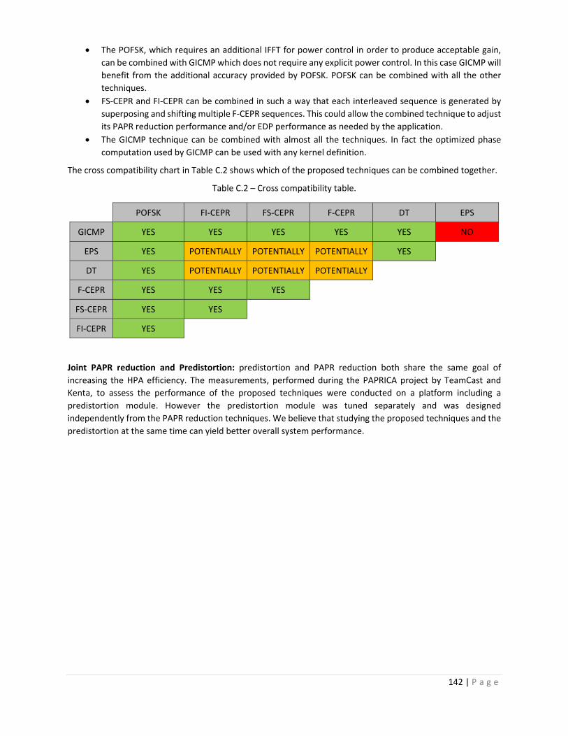
142 | P a g e
The POFSK, which requires an additional IFFT for power control in order to produce acceptable gain,
can be combined with GICMP which does not require any explicit power control. In this case GICMP will
benefit from the additional accuracy provided by POFSK. POFSK can be combined with all the other
techniques.
FS‐CEPR and FI‐CEPR can be combined in such a way that each interleaved sequence is generated by
superposing and shifting multiple F‐CEPR sequences. This could allow the combined technique to adjust
its PAPR reduction performance and/or EDP performance as needed by the application.
The GICMP technique can be combined with almost all the techniques. In fact the optimized phase
computation used by GICMP can be used with any kernel definition.
The cross compatibility chart in Table C.2 shows which of the proposed techniques can be combined together.
Table C.2 – Cross compatibility table.
POFSK FI‐CEPR FS‐CEPR F‐CEPR DT EPS
GICMP YES YES YES YES YES NO
EPS YES POTENTIALLY POTENTIALLY POTENTIALLY YES
DT YES POTENTIALLY POTENTIALLY POTENTIALLY
F‐CEPR YES YES YES
FS‐CEPR YES YES
FI‐CEPR YES
Joint PAPR reduction and Predistortion: predistortion and PAPR reduction both share the same goal of
increasing the HPA efficiency. The measurements, performed during the PAPRICA project by TeamCast and
Kenta, to assess the performance of the proposed techniques were conducted on a platform including a
predistortion module. However the predistortion module was tuned separately and was designed
independently from the PAPR reduction techniques. We believe that studying the proposed techniques and the
predistortion at the same time can yield better overall system performance.

143 | P a g e
List of Figures
Figure 1 – Fluctuations de puissance. ..................................................................................................................... II Figure 2 – Cartographie de déploiement des standards de télévision numérique terrestre dans le monde........ III Figure 3 – Caractéristique AM/AM. ....................................................................................................................... IV Figure 4 – Efficacité énergétique. .......................................................................................................................... IV Figure 5 – Signal à fluctuations élevées. ................................................................................................................. V Figure 6 – Signal à faibles fluctuations. ................................................................................................................... V Figure 7 – La technique Tone Reservation. ............................................................................................................ VI Figure 8 – Diagramme de PC=DVB‐T. .................................................................................................................... VII Figure 9 – Diagramme de PC=SYMB. ..................................................................................................................... VII Figure 10 – MER 2K. ............................................................................................................................................. VIII Figure 11 – MER 32K. ........................................................................................................................................... VIII Figure 12 – GPOFSK avec 2 et 3. ............................................................................. IX Figure 13 – GPOFSK avec 3 et 1. ............................................................................. IX Figure 14 – Diagramme de GPOFSK. ...................................................................................................................... IX Figure 15 – MER pour GPOSK en mode 2K pour différente valeurs de , 2, PC=SYMB, et
30 itérations. ...................................................................................................................................... X Figure 16 – choisit égale à l’amplitude du 5ème pique avec 4. .......................................................... X Figure 17 – Détails des itérations de la technique EPS. ......................................................................................... XI Figure 18 – Diagramme d’EPS combinée DT. ........................................................................................................ XII Figure 19 – MER pour EPS combinée avec DT en mode 32K. ............................................................................... XII Figure 20 – Relation entre les itérations et les noyaux ICMP. ............................................................................. XIII Figure 21 – Diagramme de la technique ICMP et de TR PC=DVB‐T2. ................................................................... XV Figure 22 – MER pour ICMP pour différentes valeurs de en mode 2K. ............................................................. XV Figure 23 – Diagramme de la technique ICMP. .................................................................................................... XVI Figure 24 – Performances MER pour la technique GICMP en mode 32K. .......................................................... XVII Figure 25 – Loi géométrique pour les pilotes de CEPR. ..................................................................................... XVIII Figure 26 – Schéma bloc de la technique CEPR. .................................................................................................. XIX Figure 27 – Séquences FS‐CEPR pour 2 et 2. ..................................................................................... XX Figure 28 – Séquence FI‐CEPR pour =16 et différentes valeurs d’ . ............................................................... XX Figure 29 – Diagramme de la solution F‐CEPR. ................................................................................................... XXI Figure 30 – Diagramme de la solution FS‐CEPR. ................................................................................................. XXI Figure 31 – Diagramme de la solution FI‐CEPR. .................................................................................................. XXI
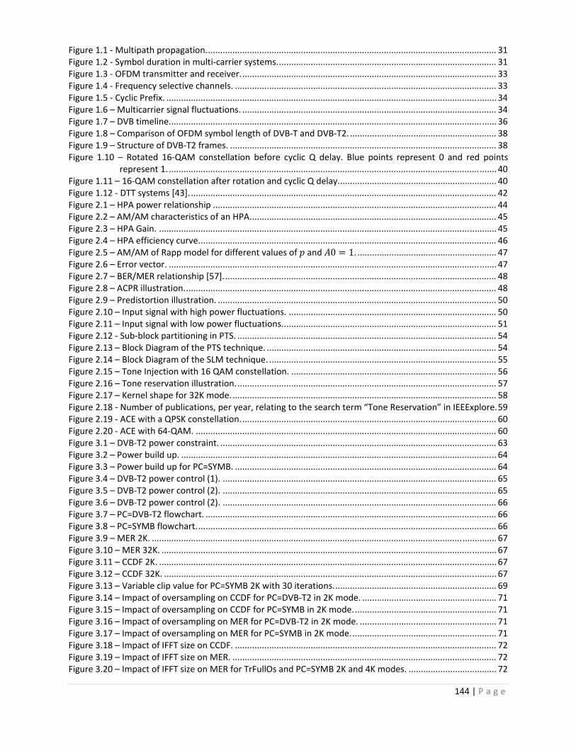
144 | P a g e
Figure 1.1 ‐ Multipath propagation. ...................................................................................................................... 31 Figure 1.2 ‐ Symbol duration in multi‐carrier systems. ......................................................................................... 31 Figure 1.3 ‐ OFDM transmitter and receiver. ........................................................................................................ 33 Figure 1.4 ‐ Frequency selective channels. ........................................................................................................... 33 Figure 1.5 ‐ Cyclic Prefix. ....................................................................................................................................... 34 Figure 1.6 – Multicarrier signal fluctuations. ........................................................................................................ 34 Figure 1.7 – DVB timeline. ..................................................................................................................................... 36 Figure 1.8 – Comparison of OFDM symbol length of DVB‐T and DVB‐T2. ............................................................ 38 Figure 1.9 – Structure of DVB‐T2 frames. ............................................................................................................. 38 Figure 1.10 – Rotated 16‐QAM constellation before cyclic Q delay. Blue points represent 0 and red points
represent 1. ...................................................................................................................................... 40 Figure 1.11 – 16‐QAM constellation after rotation and cyclic Q delay. ................................................................ 40 Figure 1.12 ‐ DTT systems [43]. ............................................................................................................................. 42 Figure 2.1 – HPA power relationship .................................................................................................................... 44 Figure 2.2 – AM/AM characteristics of an HPA. .................................................................................................... 45 Figure 2.3 – HPA Gain. .......................................................................................................................................... 45 Figure 2.4 – HPA efficiency curve. ......................................................................................................................... 46 Figure 2.5 – AM/AM of Rapp model for different values of and 0 1. ......................................................... 47 Figure 2.6 – Error vector. ...................................................................................................................................... 47 Figure 2.7 – BER/MER relationship [57]. ............................................................................................................... 48 Figure 2.8 – ACPR illustration. ............................................................................................................................... 48 Figure 2.9 – Predistortion illustration. .................................................................................................................. 50 Figure 2.10 – Input signal with high power fluctuations. ..................................................................................... 50 Figure 2.11 – Input signal with low power fluctuations. ....................................................................................... 51 Figure 2.12 ‐ Sub‐block partitioning in PTS. .......................................................................................................... 54 Figure 2.13 – Block Diagram of the PTS technique. .............................................................................................. 54 Figure 2.14 – Block Diagram of the SLM technique. ............................................................................................. 55 Figure 2.15 – Tone Injection with 16 QAM constellation. .................................................................................... 56 Figure 2.16 – Tone reservation illustration. .......................................................................................................... 57 Figure 2.17 – Kernel shape for 32K mode. ............................................................................................................ 58 Figure 2.18 ‐ Number of publications, per year, relating to the search term “Tone Reservation” in IEEExplore. 59 Figure 2.19 ‐ ACE with a QPSK constellation. ........................................................................................................ 60 Figure 2.20 ‐ ACE with 64‐QAM. ........................................................................................................................... 60 Figure 3.1 – DVB‐T2 power constraint. ................................................................................................................. 63 Figure 3.2 – Power build up. ................................................................................................................................. 64 Figure 3.3 – Power build up for PC=SYMB. ........................................................................................................... 64 Figure 3.4 – DVB‐T2 power control (1). ................................................................................................................ 65 Figure 3.5 – DVB‐T2 power control (2). ................................................................................................................ 65 Figure 3.6 – DVB‐T2 power control (2). ................................................................................................................ 66 Figure 3.7 – PC=DVB‐T2 flowchart. ....................................................................................................................... 66 Figure 3.8 – PC=SYMB flowchart. .......................................................................................................................... 66 Figure 3.9 – MER 2K. ............................................................................................................................................. 67 Figure 3.10 – MER 32K. ......................................................................................................................................... 67 Figure 3.11 – CCDF 2K. .......................................................................................................................................... 67 Figure 3.12 – CCDF 32K. ........................................................................................................................................ 67 Figure 3.13 – Variable clip value for PC=SYMB 2K with 30 iterations. .................................................................. 69 Figure 3.14 – Impact of oversampling on CCDF for PC=DVB‐T2 in 2K mode. ....................................................... 71 Figure 3.15 – Impact of oversampling on CCDF for PC=SYMB in 2K mode. .......................................................... 71 Figure 3.16 – Impact of oversampling on MER for PC=DVB‐T2 in 2K mode. ........................................................ 71 Figure 3.17 – Impact of oversampling on MER for PC=SYMB in 2K mode. ........................................................... 71 Figure 3.18 – Impact of IFFT size on CCDF. ........................................................................................................... 72 Figure 3.19 – Impact of IFFT size on MER. ............................................................................................................ 72 Figure 3.20 – Impact of IFFT size on MER for TrFullOs and PC=SYMB 2K and 4K modes. .................................... 72

145 | P a g e
Figure 3.21 – Impact of IFFT size on MER for TrFullOs and PC=SYMB 8K and 16K modes. .................................. 73 Figure 3.22 – Impact of IFFT size on MER for TrFullOs and PC=SYMB 32K mode. ................................................ 73 Figure 3.23 – Relation between IFFT size and required number of iterations for TrFullOs and PC=SYMB. ......... 74 Figure 3.24 – Relation between IFFT size and required number of iterations PC=DVB‐T2. ................................. 75 Figure 3.25 – Impact of HPA non linearity on TR algorithm, 32K mode. .............................................................. 76 Figure 3.26 – CCDF for SOCP and TR without power control (PC=NO). ................................................................ 77 Figure 3.27 – CCDF for SOCP and TR with PC=SYMB. ........................................................................................... 77 Figure 3.28 – Impact of oversampling on CCDF for SOCP with PC=SYMB. ........................................................... 78 Figure 3.29 – Completely oversampled signal ...................................................................................................... 79 Figure 3.30 – Partially oversampled signal. .......................................................................................................... 79 Figure 3.31 – Kernel choice. .................................................................................................................................. 80 Figure 3.32 – CCDF comparison for TR and POFSK, 2K mode. .............................................................................. 81 Figure 3.33 – Partial oversampled signal with 2 and 3 .......................................... 81 Figure 3.34 – Partial oversampled signal with 3 and 1 .......................................... 81 Figure 3.35 – CCDF for GPOSK with variable , 2, PC=SYMB, 10 and mode 2K.
.......................................................................................................................................................... 84 Figure 3.36 – MER for GPOSK with variable , 2, PC=SYMB, 10 and mode 2K.
.......................................................................................................................................................... 84 Figure 3.37 – MER for GPOSK with variable , 2, PC=SYMB, 30 and mode 2K.
.......................................................................................................................................................... 85 Figure 3.38 – High value. ............................................................................................................................. 85 Figure 3.39 – set to the amplitude of the 1 initial peak with 4. .................................... 85 Figure 3.40 – Low value, arrows show unnecessary peak reduction.......................................................... 86 Figure 3.41 – TR with Dynamic Threshold and 20 and variable number of iterations, mode 2K. .. 87 Figure 3.42 – TrFullOs with Dynamic Threshold and =20 and variable number of iterations, mode 2K.
.......................................................................................................................................................... 87 Figure 3.43 – EPS iteration details. ....................................................................................................................... 88 Figure 3.44 – EPS and Dynamic Vclip flowchart. ................................................................................................... 89 Figure 3.45 – TR with EPS in 2K mode and variable number of iterations. .......................................................... 89 Figure 3.46 – TrFullOs with EPS in 2K mode and variable number of iterations. ................................................. 90 Figure 3.47 – TrFullOs with EPS‐DT in 2K mode and =20. ..................................................................... 90 Figure 3.48 – TrFullOs with EPS‐DT in 32K mode and =120. ................................................................. 91 Figure 4.1 – Relation between kernel definition and number of iteration count. ............................................... 94 Figure 4.2 – MER for ICSP for 2K mode. ................................................................................................................ 94 Figure 4.3 – Flow charts for ICMP and PC=DVB‐T2. .............................................................................................. 97 Figure 4.4 – ICMP with variable sensitivity 2K. ..................................................................................................... 99 Figure 4.5 – ICMP with variable sensitivity 8K. ..................................................................................................... 99 Figure 4.6 – ICMP with variable sensitivity 32K. ................................................................................................... 99 Figure 4.7 – Grouped ICMP flowchart................................................................................................................. 100 Figure 4.8 – MER GICMP performance for 32K mode. ....................................................................................... 103 Figure 4.9 – First Test bench diagram. ................................................................................................................ 104 Figure 4.10 – Module integrating the Signal Generator and the pre‐distorter. ................................................. 105 Figure 4.11 – MER v/s time during Convergence without PAPR reduction. ....................................................... 105 Figure 4.12 – MER during Convergence with PC=SYMB. .................................................................................... 106 Figure 4.13 – MER v/s time during Convergence with EPS‐DT. .......................................................................... 106 Figure 4.14 – MER v/s time during Convergence with GICMP. ........................................................................... 106 Figure 4.15 – MER v/s time measurements with Class AB test amplifier. .......................................................... 107 Figure 4.16 – MER v/s time measurements with DOHERTY amplifier. ............................................................... 108 Figure 4.17 – View of the test with the Kenta amplifier. .................................................................................... 108 Figure 4.18 – Test bench block diagram. ............................................................................................................ 109 Figure 4.19 – Kenta Amplifier block diagram. ..................................................................................................... 109 Figure 4.20 – Output spectrum with PAPR reduction. ........................................................................................ 110 Figure 4.21 – Parallel architecture for GICMP‐G=8. ............................................................................................ 110

146 | P a g e
Figure 5.1 – Multiplicative law scheme. ............................................................................................................. 115 Figure 5.2 – Conventional channel estimation scheme. ..................................................................................... 116 Figure 5.3 – Blind channel estimation scheme. .................................................................................................. 117 Figure 5.4 – CEPR block diagram. ........................................................................................................................ 118 Figure 5.5 – F‐CEPR sequence in time domain for =256 and =16, 32, 64. .................................................... 121 Figure 5.6 – F‐CEPR sequence in time domain for =256, =32 and different values of . ............................. 121 Figure 5.7 – F‐CEPR pilot sequence generation algorithm.................................................................................. 123 Figure 5.8 – Fast Shifted CEPR with 2 and 2. ................................................................................... 125 Figure 5.9 – FS‐CEPR flowchart. .......................................................................................................................... 125 Figure 5.10 –Fast Interleaved CEPR for M=16 and different values of IO .......................................................... 129 Figure 5.11 – FI‐CEPR flowchart. ......................................................................................................................... 130 Figure 5.12 – PAPR effective gain. ...................................................................................................................... 132 Figure 5.13 – PAPR effective gain as a function of for F‐CEPR, =2048. ......................................................... 132 Figure 5.14 – for CEPR. ......................................................................................................................... 133 Figure 5.15 – for variable values of . .................................................................................................. 133 Figure 5.16 – for various values of . .................................................................................................. 134 Figure 5.17 – for various values of . .................................................................................................. 134 Figure 5.18 – for various values of . ................................................................................................... 134 Figure 5.19 – for various values of . ................................................................................................... 134 Figure 5.20 – PAPR effective gain as a function of for FS‐CEPR, =3, =10. ............................................... 135 Figure 5.21 – PAPR effective gain as a function of for FI‐CEPR =8. ............................................................. 136 Figure 5.22 – ). ......................................................................................................................................... 136 Figure 5.23 – ). ........................................................................................................................................ 137

147 | P a g e
List of Tables
Table 1 – Comparaison entre DVB‐T et DVB‐T2. .................................................................................................... III Table 2 – Puissance utilisée et nombre d’itérations effectuées en mode 32K. .................................................... XI Table 3 – Différentes configurations possibles pour GICMP en mode 32K. ........................................................ XVI Table 4 –Résultats des mesures MER. ................................................................................................................ XVII Table 5 – Gain en MER pour différentes contraintes de puissance. ................................................................... XVII Table 6 – Comparaison entre CEPR, F‐CEPR, FS‐CEPR et FI‐CEPR. ....................................................................... XXI Table 7 – Comparaison. ......................................................................................................................................... 22 Table 1.1 – Major standards using OFDM. ............................................................................................................ 30 Table 1.2 – Comparison of DVB‐T and DVB‐T2. .................................................................................................... 37 Table 1.3 – Number of P2 symbols for different FFT modes. ............................................................................... 39 Table 1.4 – Scattered pilots parameters. .............................................................................................................. 41 Table 1.5 ‐ Presence of pilots in each type of symbol. .......................................................................................... 41 Table 2.1 – Linear amplifier classes. ..................................................................................................................... 46 Table 2.2 – PAPR per code word for an OFDM system with =4 using BPSK. ..................................................... 53 Table 2.3 – New constellation point candidates. .................................................................................................. 56 Table 2.4 – Comparison of PAPR reduction techniques. ...................................................................................... 62 Table 3.1 – Tone reservation algorithm parameters ............................................................................................ 68 Table 3.2 – Number of reserved tones for different OFDM modes in DVB‐T2. .................................................... 70 Table 3.3 – Pilot Patterns in DVB‐T2 for data symbols. ........................................................................................ 70 Table 3.4 – Iteration statistics 2K. ......................................................................................................................... 76 Table 3.5 – Iteration statistics 8K. ......................................................................................................................... 76 Table 3.6 – Iteration statistics 32K. ....................................................................................................................... 76 Table 3.7 – Analysis summary ............................................................................................................................... 78 Table 3.8 – Peak position of fractional shifted kernels. ........................................................................................ 79 Table 3.9 – GPOFSK additional parameters. ......................................................................................................... 82 Table 3.10 – Actual power allocated and iterations executed for different configurations for 32K mode .......... 91 Table 4.1 – Power build‐up comparison for the reserved tones. ......................................................................... 96 Table 4.2 – ICMP additional parameters............................................................................................................... 97 Table 4.3 – Various GICMP configurations in 32K mode. ................................................................................... 100 Table 4.4 – Power build‐up per reserved tone for GICMP with = 32, =8 and =4. ...................................... 101 Table 4.5 – Comparison of OKOP and GICMP. .................................................................................................... 103 Table 4.6 – Tests results for the 3 candidate algorithms. ................................................................................... 107
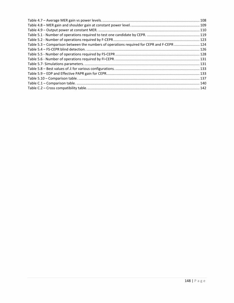
148 | P a g e
Table 4.7 – Average MER gain vs power levels. .................................................................................................. 108 Table 4.8 – MER gain and shoulder gain at constant power level. ..................................................................... 109 Table 4.9 – Output power at constant MER. ...................................................................................................... 110 Table 5.1 ‐ Number of operations required to test one candidate by CEPR. ..................................................... 119 Table 5.2 ‐ Number of operations required by F‐CEPR ....................................................................................... 123 Table 5.3 – Comparison between the numbers of operations required for CEPR and F‐CEPR .......................... 124 Table 5.4 – FS‐CEPR blind detection. .................................................................................................................. 126 Table 5.5 ‐ Number of operations required by FS‐CEPR ..................................................................................... 128 Table 5.6 ‐ Number of operations required by FI‐CEPR. ..................................................................................... 131 Table 5.7‐ Simulations parameters. .................................................................................................................... 131 Table 5.8 – Best values of for various configurations. ..................................................................................... 133 Table 5.9 – EDP and Effective PAPR gain for CEPR.............................................................................................. 133 Table 5.10 – Comparison table. .......................................................................................................................... 137 Table C.1 – Comparison table. ............................................................................................................................ 140 Table C.2 – Cross compatibility table. ................................................................................................................. 142

149 | P a g e
Bibliography
[1] "DigiWorld Research," [Online]. Available: http://www.idate.org/.
[2] S. Murray, "Digital TV World Databook," Digital TV Research, June 2015.
[3] R. Chang, "Synthesis of band‐limited orthogonal signals for multi‐channel data transmission," Bell Labs
Tech. J. 45, p. 1775–1796, 1966.
[4] R. Chang and R. Gibby, "A theoretical study of performance of an orthogonal multiplexing," IEEE Trans.
Commun., vol. 16, no. 529–340, 1968.
[5] E. P. Weinstein SB, " Data transmission by frequency‐division multiplexing using the discrete Fourier
transform," IEEE Trans. Commun., vol. 19, p. 628–634, 1971.
[6] B. Hirosaki, "An orthogonally multiplexed QAM system using the discrete Fourier transform," IEEE Trans.
Commun., vol. 29, p. 982–989, 1981.
[7] L. Cimini, "Analysis and simulation of a digital mobile radio channel using orthogonal frequency division
multiplexing," IEEE Trans. Commun., vol. 33, p. 665–675, 1985.
[8] M. Alard and R. Lassalle, "Principles of modulation and channel coding for digital broadcasting for mobile
receivers," EBU Techn. Review, vol. 224, p. 47–68, 1987.
[9] ETSI, "Radio Broadcasting Systems: Digital Audio Broadcasting (DAB) to Mobile, Portable and Fixed
Receivers,," EN300401, 2006.
[10] H. Schulze, "Stochastische Methoden und digitale Simulation von Mobilfunkkanalen," Kleinheubacher
Berichte, vol. 32, p. 473–483, 1988.

150 | P a g e
[11] P. Hoeher, "TCM on frequency‐selective land‐mobile fading channels," in 5th Tirrenia International
Workshop on Digital Communication, Tirrenia, 1991.
[12] ETSI, EN300744 2001b Digital Broadcasting Systems for Television, Sound and Data Services; Framing
Structure, Channel Coding and Modulation for Digital Terrestrial Television, 2001.
[13] J.‐F. HELARD, B. L. FLOCH, D. CASTELAIN and M. RIVIERE, " Démodulation cohérente du système de
transmission multiporteuses COFDM dans un canal de radio mobile," in Colloque GRETSI'91, 413‐417,
Juan‐les‐Pins, 16‐20 Septembre 1991.
[14] "Wireless LAN Medium Access Control (MAC) and Physical Layer (PHY) specifications: high speed physical
layer in the 5 GHz band," EEE Standard 802.11a, 1999.
[15] J. M. Cioffi, "A Multicarrier Primer," Tech. Rep. T1E1.4/91‐157, ANSI, November, 1991.
[16] "A Technical Report on High‐Bit‐Rate Digital Subscriber Lines (HDSL)," ANSI Committee T1‐
Telecommunications, Tech. Rep. 28, February 1994.
[17] "Digital Audio Broadcasting (DAB); DAB to mobile, portable and fixxed Receivers," Tech. Rep. ETSI ETS 300
401 ed.1, February 1995.
[18] "Radio Equipment and Systems (RES); HIgh PErformance Radio Local Area Network (HIPERLAN) Type 1,"
Functional specification,Tech. Rep. ETSI ETS 300 652 ed.1, October 1996.
[19] "Digital Video Broadcasting (DVB); Framing structure, channel coding and modulation for digital
terrestrial television (DVB‐T)," Tech. Rep. ETSI ETS 300 744 ed.1, March 1997.
[20] "Very‐high‐speed Digital Subscriber Lines: System Requirements," Tech. Rep. T1E1.4 VDSL SR: 98‐043R5,
ANSI, September 1998.
[21] "Transmission and Multiplexing (TM); Access transmission systems on metallic access cables; Very high
speed Digital Subscriber Line (VDSL); Part 1: Functional requirements," June 1998.
[22] "Broadband Radio Access Networks (BRAN); Inventory of broadband radio technologies and techniques,"
Tech. Rep. ETSI TR 101 173 V1.1.1, May 1998.
[23] "Wireless LAN Medium Access Control (MAC) and Physical Layer (PHY) specifications," IEEE Standard
802.11g:, 2003.
[24] "Digital Video Broadcasting (DVB); Transmission System for Handheld Terminals (DVB‐H)," ETSI standard,
November 2004.
[25] "Air Interface for Fixed Broadband Wireless Access Systems," IEEE Standard 802.16, 2004.
[26] "Wireless LAN Medium Access Control (MAC)," IEEE Candidate Standard 802.11n, 2004.

151 | P a g e
[27] "Wireless Medium Access Control (MAC) and Physical Layer (PHY) specifications for high rate Wireless
Personal Area Networks (WPANs) involving imaging and multimedia," IEEE Candidate Standard
802.15.3a, 2004.
[28] M. Yabusaki, "Asia Pacific Viewpoint and Activities: Introduction," in 4G Forum, London, UK, May 2003.
[29] S. Haykin, "Chapter 6 ‐ Base band shaping for Data Transmission," in Digital Communications 5th ed., John
Wiley & sons, 2004, pp. 245‐251.
[30] S. Haykin, "Chapter 6 ‐ An Introduction to Analog and Digital Communications," in Inter Symbol
Interference and its Cures, 6th ed., John Wiley & Sons, 2010, pp. 227‐236.
[31] C. Langton, "Inter Symbol Interference and Root Raised Cosine filtering," [Online]. Available: Available
online: www.complextoreal.com.
[32] J. Bingham, "Multicarrier modulation for data transmission: an idea whose time has come," IEEE
Communications Magazine, vol. 28, pp. 5‐14, May 1990.
[33] M. Engels, Wireless OFDM Systems: How to Make Them Work, Boston: Kluwer Academic Publishers,
2002.
[34] J. Heiskala and J. Terry, OFDM Wireless LANs: A Theoretical and Practical Guide, Indianapolis: SAMS, 2002.
[35] R. v. Nee and R. Prasad, OFDM for Wireless Multimedia Communications, Boston: Artech House
Publishers, 2000.
[36] A. S. Willsky and A. V. Oppenheim, Signals and Systems, Upper Saddle River, NJ: Prentice‐Hall, 1997.
[37] S.B. Weinstein and P.M. Ebert, "Data transmission by frequency division multiplexing using the Discrete
Fourier Transform," EEE Trans. Commun. Technol., vol. 19, no. 5, October 1971.
[38] ETSI, "Digital Video Broadcasting (DVB); Frame structure channel coding and modulation for a second
generation digital terrestrial television broadcasting system (DVB‐T2)," ETSI EN 302 755 V1.3.1, 2011.
[39] R. G. Gallager, "Low density parity‐check odes," IRE Transactions on Information Theory, vol. 8, no. 1, pp.
21‐28, 1962.
[40] D. MacKay and R. Neal, "Good codes based on very sparse matrices," Cryptography and Coding, C. Boyd,
Ed., vol. 1025 of Lecture Notes in Computer Science, p. 100–111, Springer, Berlin 1995.
[41] R. C. Base and D. K. Ray‐Chaudhuri, "On a class of error correcting binary group codes," Information and
Control, vol. 3, no. 1, pp. 68‐79, 1960.
[42] S. Alamouti, "A simple transmit diversity technique for wireless communications," IEEE Journal on
Selected areas in Communications, vol. 16, no. 8, pp. 1451‐1458, October 1998.

152 | P a g e
[43] "Digital Video Broadcasting," [Online]. Available:
https://www.dvb.org/resources/public/images/site/dvb‐t_map.pdf.
[44] M. K. Kazimierczuk, "RF Power Amplifiers," Wiley, p. November 2008.
[45] S. C. Cripps, "RF Power Amplifiers for Wireless Communications," Artech House, April 1999.
[46] W. Vereecken, W. v. Heddeghem, M. Deruyck, B. Puype, B. Lannoo, W. Joseph, D. Colle, L. Martens and
P. Demeester, "Power consumption in telecommunication networks : overview and reduction strategies,"
IEEE Communications Magazine, vol. 49, no. 6, pp. 62‐69, 2011.
[47] J. Baliga, R. Ayre, K. Hinton and a. R. Tucker, "Energy consumption in wired and wireless access networks,"
IEEE Communications Magazine, vol. 49, no. 6, pp. 70‐77, 2011.
[48] J. Palicot and Y. Louët, "A classification of methods for efficient power amplification of signals," Annales
des Télécommunications, vol. 63, pp. 351‐368, August 2008.
[49] P. B. Kenington, "High‐linearity RF amplifier design," Artech House, 2000.
[50] A. Saleh, "Frequency‐independent and frequency‐dependent nonlinear models of TWT amplifiers," IEEE
Transactions on Communications, vol. 29, no. 11, pp. 1715‐1720, 1981.
[51] M. Djamai, "Contribution à la modélisation et à la linéarisation par prédistorsion numérique adaptative
en bande de base des amplificateurs de radiocommunication," Thèse de doctorat ‐ École nationale
supérieure d'ingénieurs, Poitiers, France, 2008.
[52] J. Vuolevi, J. Manninen and T. Rahkonen, "Memory effects compensation in RF power amplifiers by using
envelope injection technique," IEEE Radio and Wireless Conference.( RAWCON), pp. 257‐260, 2001.
[53] W. H. Tranter, K. S. Shanmugan, T. S. Rappaport and K. L. Kosbar, "Principles of Communication Systems
Simulation with Wireless Applications," Prentice Hall Professional Technical Reference, January 2004.
[54] M.‐C. Chiu, C.‐H. Zeng and M.‐C. Liu, "Predistorter based on frequency domain estimation for
compensation of nonlinear distortion in OFDM systems," IEEE Transactions on Vehicular Technology, vol.
57, no. 2, pp. 882‐892, March 2008.
[55] C. Rapp, "Effects of HPA‐nonlinearity on a 4‐DPSK/OFDM‐signal for a digital sound broadcasting signal,"
Second European Conference on Satellite Communications (ECSC‐2), vol. 1, pp. 179‐184, October 1991.
[56] ETSI, "Digital Video Broadcasting (DVB); Measurement guidelines for DVB systems," ETSI TR 101 290
V1.2.1, May 2001.
[57] E. Tozer, "Broadcast Engineer’s Reference Book," Focal Press, Vols. ISBN: 978‐3540223641, 2004.
[58] B. J. Dixon, R. D. Pollard and S. Iezekiel, "A discussion of the effects of amplifier back‐off on OFDM," High
Frequency Postgraduate Student Colloquium, pp. 14‐19, Leeds, September 1999.
153 | P a g e
[59] D. Cox, "Linear amplification with nonlinear components," IEEE Transactions on Communications, vol. 22,
no. 12, pp. 1942‐1945, 1974.
[60] F. Wang, A. Yang, D. Kimball, L. Larson and P. Asbeck, "Design of wide‐bandwidth envelope‐tracking
power amplifiers for OFDM applications," IEEE Transactions on Microwave Theory and Techniques, vol.
53, no. 4, pp. 1244‐1255, 2005.
[61] D. Anderson and W. Cantrell, "High‐efficiency high‐level modulator for use in dynamic envelope tracking
cdma RF power amplifiers," IEEE MTT‐S International Microwave Symposium Digest, vol. 3, pp. 1509‐
1512, 2001.
[62] T. Arthanayake and H. Wood, ". Linear amplification using envelope feedback," Electronics Letters, vol. 7,
no. 7, pp. 145‐146, 1971.
[63] H. Seidel, H. Beurrier and A. Friedman, ". Error‐controlled high power linear amplifiers at VHF," Bell
System Technical Journal, vol. 47, no. 5, pp. 651‐722, 1968.
[64] H. S. Black, "Translating system," U.S. Patent Classification : 330/149 ; 330/124.00R, October 1928.
[65] R. Marsalek, "Contribution à la linéarisation des amplificateurs de puissance par prédistorsion numérique
adaptative en bande de base," Thèse de doctorat, Université de Marne‐la‐Vallée, France, 2003.
[66] M. Friese, "Multitone signals with low crest factor," IEEE Transactions on Communications, vol. 45, pp.
1338‐1344, October 1997.
[67] C. Tellambura, "Computation of the Continuous‐Time PAP of an OFDM Signal with BPSK Subcarriers," IEEE
Communications letters, vol. 5, no. 5, May 2001..
[68] H. Ochiai and H. Imai, "On the distribution of the peak‐to‐average power ratio in OFDM signals," IEEE
Transactions on Communications, vol. 49, pp. 282‐289, Feb. 2001.
[69] R. van Nee and A. de Wild, "Reducing the peak‐to‐average power ratio of OFDM," 48th IEEE Vehicular
Technology Conference, vol. 3, pp. 2072‐2076, 1998.
[70] X. Zhou and J. Caffery, "A new distribution bound and reduction scheme for OFDM PAPR," The 5th
International Symposium on Wireless Personal Multimedia Communications, vol. 1, pp. 158‐162, 2002.
[71] R. O'Neill and L. B. Lopes, "Envelope Variations and Spectral Splatter in Clipped Multicarrier Signals," in
Proc. IEEE PIMRC, Toronto, Canada, Sept. 1995.
[72] J. X. Li and L. J. Cimini, "Effect of Clipping and Filtering on the Performance of OFDM," IEEE Communication
Letters, vol. 2, no. 5, p. 131–133, May 1998.
[73] A. E. Jones, T. A. Wilkinson and S. K. Barton, "Block Coding Scheme for Reduction of Peak to Mean
EnvelopePower Ratio of Multicarrier Transmission Scheme," Electronics Letters, vol. 30, no. 22, p. 2098–
2099, Dec. 1994.
154 | P a g e
[74] A. E. Jones and T. A. Wilkinson, "Combined Coding for Error Control and Increased Robustness to System
Nonlinearities in OFDM," in Vehicular Technology Conference (VTC), Atlanta, GA, Apr. –May 1996.
[75] K. G. Paterson and V. Tarokh, "On the Existence and Construction of Good Codes with Low Peak‐to‐
Average Power Ratios," IEEE Trans. Info. Theory, vol. 46, no. 6, p. 1974–1987, Sept. 2000.
[76] C. V. Chong and V. Tarokh, "A Simple Encodable/Decodable OFDM QPSK Code with Low Peak to‐ Mean
Envelope Power Ratio," IEEE Trans. Info. Theory, vol. 47, no. 7, p. 3025–3029, Nov. 2001.
[77] M. Golay, "Complementary series," IEEE Transactions on Information Theory, vol. 7, no. 2, pp. 82‐87, April
1961.
[78] S. Boyd, "Multitone signals with low crest factor.," IEEE Transactions on Circuits and Systems, Vols. CAS‐
33, p. 1018–1022, October 1986.
[79] B. Popovic., "Synthesis of power efficient multitone signals with flat amplitude spectrum," IEEE
Transactions on Communications, vol. 39, no. 7, p. 1031–1033, 1991.
[80] J. A. Davis and J. Jedwab, "Peak‐to‐mean power control and error correction for OFDM transmission using
golay sequences and reed‐muller codes," IEEE Electronic Letters, vol. 33, no. 4, p. 267–26, February 1997.
[81] J. A. Davis and J. Jedwab, "Peak‐to‐mean power control in OFDM, golay complementary sequences, and
reed‐muller codes," IEEE Transactions on Information Theory, vol. 45, no. 7, p. 2397–2417, November
1999.
[82] K. Patterson, "Generalized reed‐muller codes and power control in OFDM modulation," IEEE Transactions
on Information Theory, vol. 46, no. 1, p. 104–120, January 2000.
[83] S. Huang, H. Wu, S. Chang and a. X. Liu, "Novel sequence design for low‐PMEPR and high‐code‐rate OFDM
systems," . IEEE Transactions on Communications, vol. 58, no. 2, p. 405–410, February 2010.
[84] S. H. Müller and J. B. Huber, "OFDM with Reduced Peak–to–Average Power Ratio by Optimum
Combination of Partial Transmit Sequences," Electronics Letters, vol. 33, no. 5, p. 368–369, Feb. 1997.
[85] S. H. Müller and J. B. Huber, "A Novel Peak Power Reduction Scheme for OFDM," in IEEE PIMRC '97,
Helsinki, Finland, Sept. 1997.
[86] R. W. Bäuml, R. F. H. Fisher and J. B. Huber, "Reducing the Peak‐to‐Average Power Ratio of Multicarrier
Modulation by Selected Mapping," Electronics Letters, vol. 32, no. 22, p. 2056–2057, Oct. 1996.
[87] S. H. Müller and J. B. Huber, "A Comparison of Peak Power Reduction Schemes for OFDM," in IEEE
GLOBECOM, Phoenix, AZ,USA, Nov. 1997.
[88] G. R. Hill, M. Faulkner and J. Singh, "Reducing the Peak‐to‐Average Power Ratio in OFDM by Cyclically
Shifting Partial Transmit Sequences," Electronics Letters, vol. 36, no. 6, pp. 560‐561, Mar. 2000.

155 | P a g e
[89] P. V. Eetvelt, G. Wade and M. Tomlinson, "Peak to Average Power Reduction for OFDM Schemes by
Selective Scrambling," Electronics Letters, vol. 32, no. 21, vol. 32, no. 21, p. 1963–1964, Oct. 1996.
[90] A. D. S. Jayalath and C. Tellambura, "Reducing the Peak to‐ Average Power Ratio of Orthogonal Frequency
Division Multiplexing Signal through Bit or Symbol Interleaving," Electronics Letters, vol. 36, no. 13, p.
1161–1163, June 2000.
[91] J. Tellado, Peak to Average Power Reduction for Multicarrier Modulation, Ph.D. dissertation, Stanford
Univ., 2000.
[92] J. Tellado and C. Cioffi, "PAR reduction for multicarrier transmission systems," US patent, 1997.
[93] J. Tellado, "Wireless, Multicarrier Modulation with Low PAR ‐ Applications to DSL and Wireless," Kluwer
Academic Publishers, 2000.
[94] A. Aggarwal and T. H. Meng, "A Convex Interior Point Method for Optimal OFDM PAR Reduction," IEEE
Int. Conf. on Commun., vol. 3, pp. 1985‐1990, Seoul, South Korea, May 2005.
[95] S. Zabre, J. Palicot, Y. Louet and C. Lereau, "SOCP Approach for OFDM Peak‐to‐Average Power Ratio
Reduction in the Signal Adding Context," IEEE Symp. on Sig. Proc. and Inf. Tech., Vancouver, Canada, Aug.
2006.
[96] I. Mahafeno, Y. Louet and J. Helard, "PAPR reduction method for OFDM systems using dedicated
subcarriers: a proposal for the future DVB‐T standard," 2008 IEEE International Symposium on Broadband
Multimedia Systems and Broadcasting, pp. 1‐3, 2008.
[97] I. Mahafeno, Y. Louet and J.‐F. Helard, "Peak‐to‐average power ratio reduction using second order cone
programming based tone reservation for terrestrial digital video broadcasting systems," IET
Communications, vol. 3, no. 7, pp. 1250‐1261, July 2009.
[98] M. Lobo, L. Vandenberghe, S. Boyd and H. Lebret, "Applications of second order cone programming,"
Linear Algebra and its Applications. Special Issue on Linear Algebra in Control, Signals and Image
Processing, pp. 284:193‐228, November 1998.
[99] S. Zabre, J. Palicot, Y. Louet and C. Lereau, "SOCP Approach for OFDM Peak‐to‐Average Power Ratio
Reduction in the Signal Adding Context," IEEE International Symposium on Signal Processing and
Information Technology, pp. 834 ‐ 839, Aug. 2006.
[100] D. Guel, J. Palicot and Y. Louët, "Tone reservation technique based on geometric method for orthogonal
frequency division multiplexing peak‐to‐average power ratio reduction," IET Communications, vol. 4, no.
17, p. 2065–2073, June 2010.
[101] B. Koussa, S. Bachir, C. Perrine, C. Duvanaud and R. Vauzelle, "A comparison of several gradient based
optimization algorithms for PAPR reduction in OFDM systems," 2nd International Conference on
Communications, Computing and Control Applications (CCCA), pp. 1‐6, Dec. 2012.

156 | P a g e
[102] S. Janaaththanan, C. Kasparis and B. Evans, "A Gradient Based Algorithm for PAPR Reduction of OFDM
using Tone Reservation Technique," IEEE Vehicular Technology Conference (VTC) Spring, pp. 2977‐2980,
May 2008.
[103] A. Ghassemi and T. Gulliver, "A Simplified Suboptimal Algorithm for Tone Reservation OFDM," IEEE
International Conference on Communications (ICC), pp. 1‐5, June 2009.
[104] J. Baliga, A. Grant, G. Woodward and A. Kind, "A Gradient Based Peak‐to‐Average Power Ratio Reduction
Method," Global Telecommunications Conference (GLOBECOM), pp. 3807‐3811, Nov. 2007.
[105] B. S. Krongold and D. Jones, "A new tone reservation method for complex‐baseband PAR reduction in
OFDM systems," International Conference on Acoustics, Speech, and Signal Processing (ICASSP), vol. 3,
pp. III‐2321‐III‐2324, May 2002.
[106] B. S. Krongold and D. Jones, "An active‐set approach for OFDM PAR reduction via tone reservation," IEEE
Transactions on Signal Processing, vol. 52, no. 2, pp. 495‐509, Feb. 2004.
[107] M. Wang, D. Quevedo, G. Goodwin and B. S. Krongold, "A complex‐baseband active‐set approach for tone
reservation PAR reduction in OFDM systems," Australian Communications Theory Workshop, pp. 113‐
118, Feb. 2008.
[108] W. Ling, "Shaping Quantization Noise and Clipping Distortion in Direct‐Detection Discrete Multitone," vol.
32, no. 9, pp. 1750‐1758, 2014.
[109] S. Rosati, E. Candreva and G. Corazza, "Rotation Invariant Subcarrier Mapping over DVB‐T2 Reserved
Tones,"," in Vehicular Technology Conference (VTC Spring), Dresden, Germany, 2013.
[110] T. Jiang, C. Ni, C. Xu and Q. Qi, "Curve Fitting Based Tone Reservation Method with Low Complexity for
PAPR Reduction in OFDM Systems," IEEE Communications Letters, vol. 18, no. 5, pp. 805‐808, 2014.
[111] L. Jian and Y. Wan, "An improved tone reservation method for PAPR reduction in OFDM systems," in
International Conference on Mechatronic Sciences, Electric Engineering and Computer (MEC), Shengyang,
China, 2013.
[112] H.‐T. Huang, C.‐T. Lin, H.‐C. Liu, H.‐H. Hsu, M.‐F. Wu, C.‐H. Lin, C.‐H. Li and Chia‐Chien Wei, "W‐band DD‐
OFDM‐RoF system employing pilot‐aided PAPR reduction," Microwave Photonics (MWP) and the 2014
9th Asia‐Pacific Microwave Photonics Conference (APMP), pp. 434‐437, 2014.
[113] S. Bachir, B. Koussa, C. Perrine, C. Duvanaud and R. Vauzelle, "Peak power reduction for OFDM systems
in vehicular wireless communications context," in International Conference on Electronics, Computers
and Artificial Intelligence (ECAI), Pitesti, Romania, 2013.
[114] M. Hu, Y. Li, X. Lu and H. Zhang, "Tone Reservation to Minimize Nonlinearity Impact on OFDM Signals,"
vol. PP, no. 99, p. 1, 2014.

157 | P a g e
[115] F. Harris, E. Venosa, X. Chen and C. Dick, "A reduced PAPR PR‐NMDFB based DUC architecture for transmit
downlink of combined 3GPP LTE and UMTS signals," in IEEE International Conference on Acoustics, Speech
and Signal Processing (ICASSP), Florence, Italy, 2014.
[116] J. Xia, Y. Li, Z. Zhang, M. Wang, W. Yu and Shuai Wang, "A suboptimal TR algorithm with fixed phase
rotation for papr reduction in MC‐CDMA system," in IET International Conference on Information and
Communications Technologies (IETICT),, Beijing, China, 2013.
[117] S. Tabassum, S. Hussain and A. Ghafoor, "A Novel Adaptive Mode PAPR Reduction Scheme for NC‐OFDM
Based Cognitive Radios,," in Vehicular Technology Conference (VTC Spring), Dresden, Germany, 2013.
[118] M. Yang and Y. Shin, "PAPR reduction using tone reservation for NC‐OFDM transmissions," in h
International Conference on Ubiquitous and Future Networks (ICUFN), Puket, Thailand, 2012 .
[119] T. A. Truong, H. Lin, B. Jahan, M. Arzel and M. Jezequel, "PAPR reduction using contiguous‐tone Tone
Reservation technique in optical OFDM IMDD transmissions," in Optical Fiber Communication Conference
and Exposition and the National Fiber Optic Engineers Conference (OFC/NFOEC), Anaheim, CA, USA, 2013
.
[120] N. Singh, A. Bhadu and A. Kumar, "Combined SLM and tone reservation for PAPR reduction in OFDM
systems,"," in Confluence 2013: The Next Generation Information Technology Summit, 2013.
[121] H. Asjadi, "Pre‐ and post‐IFFT PAPR reduction in pilot‐aided OFDM transmission systems," in IEEE
International Symposium on Broadband Multimedia Systems and Broadcasting (BMSB) , London, UK,
2013.
[122] B. Krongold and D. Jones, "PAR reduction in OFDM via active constellation extension," in IEEE
International Conference on Acoustics, Speech, and Signal Processing (ICASSP), Hon Kong, China, 2003.
[123] D. L. Jones, "Peak power reduction in OFDM and DMT via active channel modification," Proceedings of
the Asilomar Conference on Signals, Systems, and Compurers, vol. 2, pp. 1076‐1079, 1999.
[124] A. Gatherer and M. Poky, "Controlling clipping probability in DMT transmission," 31st Asilomar
Conference on Signals, Systems, and Computers, pp. 578‐584, 1997.
[125] B. S. Krongold and D. Jones, "PAR reduction in OFDM via active constellation extension," in IEEE
International Conference on Acoustics, Speech, and Signal Processing (ICASSP), Hon Kong, China, 2003.
[126] B. S. Krongold and D. L. Jones, "PAR Reduction in OFDM via Active Constellation Extension," IEEE Trans.
Broadcast, vol. 49, no. 3, p. 258–268, Sept. 2003.
[127] A. Hekkala, S. Boumard and M. Lasanen, "Exponential companding and active constellation extension
comparisons for PAPR reduction," 26th International Teletraffic Congress (ITC), Sept. 2014.
[128] I. Sohn, "A Low Complexity PAPR Reduction Scheme for OFDM Systems via Neural Networks," IEEE
Communications Letters, vol. 18, no. 2, pp. 225‐228, February 2014.

158 | P a g e
[129] J. He and Z. Yan, "Improving convergence rate of active constellation extension algorithm for PAPR
reduction in OFDM," IEEE International Conference on Information and Automation (ICIA), pp. 280‐284,
Aug. 2013.
[130] H.‐B. Jeon, J.‐S. No and D.‐J. Shin, " "A New PAPR Reduction Scheme Using Efficient Peak Cancellation for
OFDM Systems," IEEE Transactions on Broadcasting, vol. 58, no. 4, pp. 619‐628, Dec. 2012.
[131] K. Bae, J. Andrews and E. Powers, "Adaptive active constellation extension algorithm for peak‐to‐average
ratio reduction in OFDM," IEEE Communications Letters, vol. 14, no. 1, pp. 39‐41, January 2010.
[132] K. Bae and E. Powers, "A novel active constellation extension algorithm with low peak power for pilot‐
aided OFDM systems," IEEE International Conference on Acoustics Speech and Signal Processing (ICASSP),
pp. 3282‐3285, March 2010.
[133] C. Wang and S. H. Leung, "Par reduction in OFDM through convex programming," IEEE International
Conference on Acoustics, Speech and Signal Processing (ICASSP), pp. 3597‐3600, 2008.
[134] M. Malkin, B. Krongold and J. Cioffi, "Optimal constellation distortion for PAR reduction in OFDM
systems," IEEE 19th International Symposium on Personal, Indoor and Mobile Radio Communications
(PIMRC), pp. 1‐5, Sept. 2008.
[135] Y. Zhang and W. Tang, "OFDM PAPR reduction with digital amplitude predistortion," URSI General
Assembly and Scientific Symposium (URSI GASS), Aug. 2014.
[136] M. Brandon, M. Ariaudo, S. Traverso, J. Bouvier, I. Fijalkow and J. Gautier, "Linearity improvement thanks
to the association of Active Constellation Extension and digital predistortion for OFDM," IEEE 9th
International New Circuits and Systems Conference (NEWCAS), pp. 293‐296, June 2011.
[137] H. Luo and L. Zhou, "Optimized Gradient Projection for PAPR reduction of OFDM signals," 4th IEEE
International Conference onBroadband Network and Multimedia Technology (IC‐BNMT), pp. 118‐121,
Oct. 2011.
[138] Y. Zhou and T. Jiang, "A novel clipping integrated into ACE for PAPR reduction in OFDM systems,"
International Conference on Wireless Communications & Signal Processing, pp. 1‐4, Nov. 2009.
[139] F. Longo, R. Ansari, Y. Yao and F. Sellone, "Erasure pattern selection with active constellation extension
for peak‐to‐average power ratio reduction in OFDM," IEEE International Conference on
Electro/Information Technology, pp. 53‐58, May 2007.
[140] K. Pradeep and M. L. Sim, "PAR reduction in space‐time coded OFDM via modified active constellation
extension," IEEE Conference on Innovative Technologies in Intelligent Systems and Industrial Applications
(CITISIA) , pp. 71‐75, July 2008.
[141] B. S. Krongold, Y. Tang and W. Shieh, "Fiber nonlinearity mitigation by PAPR reduction in coherent optical
OFDM systems via active constellation extension," 34th European Conference on Optical Communication
(ECOC), pp. 1‐2, Sept. 2008.

159 | P a g e
[142] J. Doblado, A. Oria, V. Baena‐Lecuyer, P. Lopez and D. Perez‐Calderon, "Cubic Metric Reduction for DCO‐
OFDM Visible Light Communication Systems," Journal of Lightwave Technology, vol. 33, no. 10, pp.
1971,1978, May 2015.
[143] T. Detwiler and D. Jones, "OFDM Receiver Design for Active Constellation Extension," Conference Record
of the Thirty‐Ninth Asilomar Conference on Signals, Systems and Computers, pp. 1485‐1489, 2005.
[144] N. van der Neut, B. Maharaj, F. de Lange, G. Gonzalez and F. a. C. J. Gregorio, "PAPR reduction in FBMC
systems using a smart gradient‐project active constellation extension method," 21st International
Conference on Telecommunications (ICT), pp. 134‐139, May 2014.
[145] A. Louliej, Y. Jabrane, B. Said and A. Ouahman, "Reduction of power envelope fluctuations in ECMA‐368
ultra wideband communication system," nternational Conference on Multimedia Computing and Systems
(ICMCS), pp. 449‐453, May 2012.
[146] F. Hu, L. Jin, J. Li and F. Wu, "An active constellation extension architecture for STBC MIMO decoding,"
IEEE 2nd International Conference on Software Engineering and Service Science (ICSESS), pp. 128‐132, July
2011.
[147] ETSI, "Frame structure channel coding and modulation for a second generation digital terrestrial
television broadcasting system (DVB‐T2)," ETSI EN 302755 V1.1.1, Sept. 2009.
[148] M. Mroué, A. Nafkha, J. Palicot, B. Gavalda and N. Dagorne, "Performance and Implementation Evaluation
of TR PAPR Reduction Methods for DVB‐T2," International Journal of Digital Multimedia Broadcasting,
2010.
[149] X. Wang, Y. Wu and H.‐C. Wu, "Iterative channel estimation and papr reduction for ofdm system with
overlay watermarks," in IEEE GLOBECOM, 2006.
[150] C. Li and W.‐C. Huang, "Semi‐Blind Channel Estimation Using Superimposed Training Sequences with
Constant Magnitude in Dual Domain for OFDM Systems," VTC Spring, pp. 1575‐1579, 2006.
[151] L. Guan, T. Jiang, D. Qu and Y. Zhou, "Joint Channel Estimation and PTS to Reduce Peak‐to‐Average‐Power
Radio in OFDM Systems Without Side Information," IEEE Signal Process. Lett., vol. 17, no. 10, pp. 883‐
886, Oct. 2010.
[152] K. Long, Y. Fu and Y. Wang, "The Contradiction Between Channel Estimation and PAPR Performance in
Cyclic Shift PTS," IEEE BMEI'2012, pp. 1525‐1528, Oct. 2012.
[153] A. Ho, Y. Nasser, J.‐F. Helard and Y. Louet, "On the Performance of Joint Channel Estimation and PAPR
Reduction Scheme," Proc. Of IEEE International Conference on Computing, Networking and
Communications, pp. 1‐6, January 2012.
[154] A. Ho, J.‐F. Helard, Y. Nasser and Y. Louet, "PAPR Reduction Approach Based on Channel Estimation Pilots
for Next Generations Broadcasting Systems," Eurasip Int. Journal on Digital and Multimedia Broadcasting
‐ Article ID 365896, 2011.

160 | P a g e
[155] A. Ho, J.‐F. Helard and Y. Nasser, "A Novel Combined PAPR Reduction and Channel Estimation Approach
for OFDM Systems," IEEE BMSB, pp. 1‐5, May 2010, Shanghai, China.
[156] A. Ghassemi and T. Gulliver, "PAPR reduction in OFDM based cognitive radio with blockwise‐subcarrier
activation,"," in International Conference on Communications (ICC), Ottawa, Canada, 2012.
[157] D. Jones, "Peak power reduction in OFDM and DMT via active channel modification," in Asilomar
Conference on Signals, Systems, and Computers, USA, 1999.
[158] ETSI, "TR 102 831 V1.2.1 (2012‐08). Digital Video Broadcasting (DVB); Implementation guidelines for a
second generation digital terrestrial television broadcasting system (DVB‐T2)," 2012.
[159] N. Rahim, H. Dao, M. Islam and A. Ibrahim, ""Prediction of the tropospheric scintillation for earth to
satellite link in tropical climate,"," in Mechatronics (ICOM), 2011 4th International Conference On, Kuala
Lumpur, Malaysia, May 2011.
[160] P. B. Kenington, "High‐linearity RF amplifier design," Artech House, 2000.
[161] M. K. Kazimierczuk, "RF Power Ampliersfi," Wiley, November 2008.
[162] J. Wang, Z. Liu, Z. Luo and Z. Wang, "A novel peak‐to‐average power ratio reduction method for amplitude
phase shift keying," Computing, Communications and IT Applications Conference (ComComAp), vol. 2013,
pp. 100‐104, April 2013.
[163] A. Al‐Rabah, M. Masood, A. Ali and T. Al‐Naffouri, "Receiver‐based Bayesian PAPR reduction in OFDM,"
in 21st European Signal Processing Conference (EUSIPCO), 2013.
[164] IEEE, 802.11a Wireless LAN Medium Access Control (MAC) and Physical Layer (PHY) specifications: High
Speed Physical Layer in the 5 GHz Band.
[165] "COST 207 Report, Digital land mobile radio communications," Commission of European Communities,
Directorate General, Telecommunications Information Industries and Innovation, Luxemburg, 1989.

161 | P a g e
Annex A – Reserved pilots positions
IFFT Size
# of reserved tones
Reserved tone positions for data symbols
1K 10 109, 117, 122, 129, 139, 321, 350, 403, 459, 465
2K 18 250, 404, 638, 677, 700, 712, 755, 952, 1125, 1145, 1190, 1276, 1325, 1335, 1406, 1431, 1472,1481
4K 36 170, 219, 405, 501, 597, 654, 661, 745, 995, 1025, 1319, 1361, 1394, 1623, 1658, 1913, 1961, 1971, 2106, 2117, 2222, 2228, 2246, 2254, 2361, 2468, 2469, 2482, 2637, 2679, 2708, 2825, 2915, 2996, 3033, 3119
8K 72
111, 115, 123, 215, 229, 392, 613, 658, 831, 842, 997, 1503, 1626, 1916, 1924, 1961, 2233, 2246, 2302, 2331, 2778, 2822, 2913, 2927, 2963, 2994, 3087, 3162, 3226, 3270, 3503, 3585, 3711, 3738, 3874, 3902, 4013, 4017, 4186, 4253, 4292, 4339, 4412, 4453, 4669, 4910, 5015, 5030, 5061, 5170, 5263, 5313, 5360, 5384, 5394, 5493, 5550, 5847, 5901, 5999, 6020, 6165, 6174, 6227, 6245, 6314, 6316, 6327, 6503, 6507, 6545, 6565
16K 144
109, 122, 139, 171, 213, 214, 251, 585, 763, 1012, 1021, 1077, 1148, 1472, 1792, 1883, 1889, 1895, 1900, 2013, 2311, 2582, 2860, 2980, 3011, 3099, 3143, 3171, 3197, 3243, 3257, 3270, 3315, 3436, 3470, 3582, 3681, 3712, 3767, 3802, 3979, 4045, 4112, 4197, 4409, 4462, 4756, 5003, 5007, 5036, 5246, 5483, 5535, 5584, 5787, 5789, 6047, 6349, 6392, 6498, 6526, 6542, 6591, 6680, 6688, 6785, 6860, 7134, 7286, 7387, 7415, 7417, 7505, 7526, 7541, 7551, 7556, 7747, 7814, 7861, 7880, 8045, 8179, 8374, 8451, 8514, 8684, 8698, 8804, 8924, 9027, 9113, 9211, 9330, 9479, 9482, 9487, 9619, 9829, 10326, 10394, 10407, 10450, 10528, 10671, 10746, 10774, 10799, 10801, 10912, 11113, 11128, 11205, 11379, 11459, 11468, 11658, 11776, 11791, 11953, 11959, 12021, 12028, 12135, 12233, 12407, 12441, 12448, 12470, 12501,
32K 288
164, 320, 350, 521, 527, 578, 590, 619, 635, 651, 662, 664, 676, 691, 723, 940, 1280, 1326, 1509, 1520, 1638, 1682, 1805, 1833, 1861, 1891, 1900, 1902, 1949, 1967, 1978, 1998, 2006, 2087, 2134, 2165, 2212, 2427, 2475, 2555, 2874, 3067, 3091, 3101, 3146, 3188, 3322, 3353, 3383, 3503, 3523, 3654, 3856, 4150, 4158, 4159, 4174, 4206, 4318, 4417, 4629, 4631, 4875, 5104, 5106, 5111, 5131, 5145, 5146, 5177, 5181, 5246, 5269, 5458, 5474, 5500, 5509, 5579, 5810, 5823, 6058, 6066, 6098, 6411, 6741, 6775, 6932, 7103, 7258, 7303, 7413, 7586, 7591, 7634, 7636, 7655, 7671, 7675, 7756, 7760, 7826, 7931, 7937, 7951, 8017, 8061, 8071, 8117, 8317, 8321, 8353, 8806, 9010, 9237, 9427, 9453, 9469, 9525, 9558, 9574, 9584, 9820, 9973, 10011, 10043, 10064, 10066, 10081, 10136, 10193, 10249, 10511, 10537, 11083, 11350, 11369, 11428, 11622, 11720, 11924, 11974, 11979, 12944, 12945, 13009, 13070, 13110, 13257, 13364, 13370, 13449, 13503, 13514, 13520, 13583, 13593, 13708, 13925, 14192, 14228, 14235, 14279, 14284, 14370, 14393, 14407, 14422, 14471, 14494, 14536, 14617, 14829, 14915, 15094, 15138, 15155, 15170, 15260, 15283, 15435, 15594, 15634, 15810, 16178, 16192, 16196, 16297, 16366, 16498, 16501, 16861, 16966, 17039, 17057, 17240, 17523, 17767, 18094, 18130, 18218, 18344, 18374, 18657, 18679, 18746, 18772, 18779, 18786, 18874, 18884, 18955, 19143, 19497, 19534, 19679, 19729, 19738, 19751, 19910, 19913, 20144, 20188, 20194, 20359, 20490, 20500, 20555, 20594, 20633, 20656, 21099, 21115, 21597, 22139, 22208, 22244, 22530, 22547, 22562, 22567, 22696, 22757, 22798, 22854, 22877, 23068, 23102, 23141, 23154, 23170, 23202, 23368, 23864, 24057, 24215, 24219, 24257, 24271, 24325, 24447, 25137, 25590, 25702, 25706, 25744, 25763, 25811, 25842, 25853, 25954, 26079, 26158, 26285, 26346, 26488
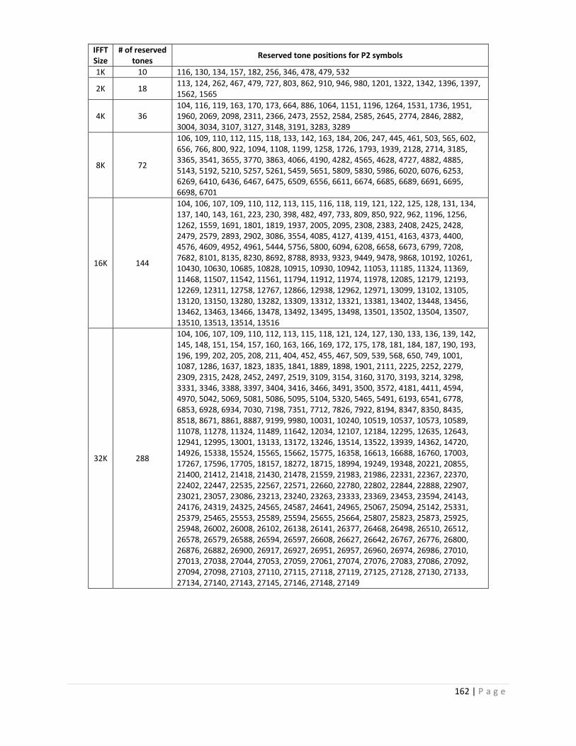
162 | P a g e
IFFT Size
# of reserved tones
Reserved tone positions for P2 symbols
1K 10 116, 130, 134, 157, 182, 256, 346, 478, 479, 532
2K 18 113, 124, 262, 467, 479, 727, 803, 862, 910, 946, 980, 1201, 1322, 1342, 1396, 1397, 1562, 1565
4K 36 104, 116, 119, 163, 170, 173, 664, 886, 1064, 1151, 1196, 1264, 1531, 1736, 1951, 1960, 2069, 2098, 2311, 2366, 2473, 2552, 2584, 2585, 2645, 2774, 2846, 2882, 3004, 3034, 3107, 3127, 3148, 3191, 3283, 3289
8K 72
106, 109, 110, 112, 115, 118, 133, 142, 163, 184, 206, 247, 445, 461, 503, 565, 602, 656, 766, 800, 922, 1094, 1108, 1199, 1258, 1726, 1793, 1939, 2128, 2714, 3185, 3365, 3541, 3655, 3770, 3863, 4066, 4190, 4282, 4565, 4628, 4727, 4882, 4885, 5143, 5192, 5210, 5257, 5261, 5459, 5651, 5809, 5830, 5986, 6020, 6076, 6253, 6269, 6410, 6436, 6467, 6475, 6509, 6556, 6611, 6674, 6685, 6689, 6691, 6695, 6698, 6701
16K 144
104, 106, 107, 109, 110, 112, 113, 115, 116, 118, 119, 121, 122, 125, 128, 131, 134, 137, 140, 143, 161, 223, 230, 398, 482, 497, 733, 809, 850, 922, 962, 1196, 1256, 1262, 1559, 1691, 1801, 1819, 1937, 2005, 2095, 2308, 2383, 2408, 2425, 2428, 2479, 2579, 2893, 2902, 3086, 3554, 4085, 4127, 4139, 4151, 4163, 4373, 4400, 4576, 4609, 4952, 4961, 5444, 5756, 5800, 6094, 6208, 6658, 6673, 6799, 7208, 7682, 8101, 8135, 8230, 8692, 8788, 8933, 9323, 9449, 9478, 9868, 10192, 10261, 10430, 10630, 10685, 10828, 10915, 10930, 10942, 11053, 11185, 11324, 11369, 11468, 11507, 11542, 11561, 11794, 11912, 11974, 11978, 12085, 12179, 12193, 12269, 12311, 12758, 12767, 12866, 12938, 12962, 12971, 13099, 13102, 13105, 13120, 13150, 13280, 13282, 13309, 13312, 13321, 13381, 13402, 13448, 13456, 13462, 13463, 13466, 13478, 13492, 13495, 13498, 13501, 13502, 13504, 13507, 13510, 13513, 13514, 13516
32K 288
104, 106, 107, 109, 110, 112, 113, 115, 118, 121, 124, 127, 130, 133, 136, 139, 142, 145, 148, 151, 154, 157, 160, 163, 166, 169, 172, 175, 178, 181, 184, 187, 190, 193, 196, 199, 202, 205, 208, 211, 404, 452, 455, 467, 509, 539, 568, 650, 749, 1001, 1087, 1286, 1637, 1823, 1835, 1841, 1889, 1898, 1901, 2111, 2225, 2252, 2279, 2309, 2315, 2428, 2452, 2497, 2519, 3109, 3154, 3160, 3170, 3193, 3214, 3298, 3331, 3346, 3388, 3397, 3404, 3416, 3466, 3491, 3500, 3572, 4181, 4411, 4594, 4970, 5042, 5069, 5081, 5086, 5095, 5104, 5320, 5465, 5491, 6193, 6541, 6778, 6853, 6928, 6934, 7030, 7198, 7351, 7712, 7826, 7922, 8194, 8347, 8350, 8435, 8518, 8671, 8861, 8887, 9199, 9980, 10031, 10240, 10519, 10537, 10573, 10589, 11078, 11278, 11324, 11489, 11642, 12034, 12107, 12184, 12295, 12635, 12643, 12941, 12995, 13001, 13133, 13172, 13246, 13514, 13522, 13939, 14362, 14720, 14926, 15338, 15524, 15565, 15662, 15775, 16358, 16613, 16688, 16760, 17003, 17267, 17596, 17705, 18157, 18272, 18715, 18994, 19249, 19348, 20221, 20855, 21400, 21412, 21418, 21430, 21478, 21559, 21983, 21986, 22331, 22367, 22370, 22402, 22447, 22535, 22567, 22571, 22660, 22780, 22802, 22844, 22888, 22907, 23021, 23057, 23086, 23213, 23240, 23263, 23333, 23369, 23453, 23594, 24143, 24176, 24319, 24325, 24565, 24587, 24641, 24965, 25067, 25094, 25142, 25331, 25379, 25465, 25553, 25589, 25594, 25655, 25664, 25807, 25823, 25873, 25925, 25948, 26002, 26008, 26102, 26138, 26141, 26377, 26468, 26498, 26510, 26512, 26578, 26579, 26588, 26594, 26597, 26608, 26627, 26642, 26767, 26776, 26800, 26876, 26882, 26900, 26917, 26927, 26951, 26957, 26960, 26974, 26986, 27010, 27013, 27038, 27044, 27053, 27059, 27061, 27074, 27076, 27083, 27086, 27092, 27094, 27098, 27103, 27110, 27115, 27118, 27119, 27125, 27128, 27130, 27133, 27134, 27140, 27143, 27145, 27146, 27148, 27149

163 | P a g e
Annex B – Time domain derivation for F‐CEPR
sequences
The time domain representation of s is given by:
1
√.
For CEPR the pilots are uniformly distributed and can be expresses follows:
0
0
Variable change becomes
1
√.
1
√λ .
λ
√
Let
If is a multiple of
.2
Then
.
if ( 0, then
if ( 0, then becomes the sum of a geometric series of ratio and first term 1.
1
1
1
10
Then
λM
√. .
λM
√ 0
0


165 | P a g e

166 | P a g e
Résumé
La technique Orthogonal Frequency Division Multiplexing (OFDM) a été adoptée par plusieurs systèmes de télécommunications et de diffusion pour sa robustesse, sa capacité à transmettre de hauts débits dans des canaux radio-mobiles et pour son efficacité spectrale. Cependant, les signaux OFDM sont caractérisés par des fluctuations importantes, mesurées par le rapport de la puissance crête sur la puissance moyenne (Peak to Average Power Ratio – PAPR) du signal, qui génèrent des distorsions à la sortie de l’amplificateur non-linéaire de puissance (High Power Amplifier - HPA) et ne permettent pas de l’utiliser dans sa zone optimale afin de diminuer sa consommation énergétique. La deuxième génération de la norme Digital Video Broadcasting (DVB-T2) a notamment adopté la technique Tone Reservation (TR) de réduction du PAPR. Son principe consiste à créer un noyau, à partir d’un ensemble de sous-porteuses réservées, qui est ensuite ajouté d’une manière itérative au signal OFDM de façon à réduire les pics du signal et donc son PAPR.
Dans la première partie de la thèse, différents algorithmes permettant d’améliorer les performances de cette solution TR DVT-T2 sont proposés. Un premier groupe de solutions, reposant sur la même définition du noyau, comprend : la technique Partial Oversampling and Fractional Shifted Kernels (POFSK) reposant sur un sur-échantillonnage partiel du signal, la technique Dynamic Threshold (DT) qui effectue un calcul dynamique du seuil de troncature et la technique Enhanced Peak Selection (EPS) qui améliore la sélection des pics à réduire. Le deuxième groupe de solutions comprend tout d’abord la technique Individual Carrier Multiple Peaks (ICMP) qui repose sur une nouvelle définition du noyau et utilise un calcul de phase différent permettant la réduction de plusieurs pics en même temps. La technique GICMP est une version optimisée de la technique ICMP qui, en parallélisant les opérations, permet de réduire le délai de traitement et le nombre total d’itérations. Les résultats de simulations et les mesures effectuées sur une plateforme de transmission réelle montrent que, par rapport à la version TR de DVB-T2, l’algorithme GICMP offrait notamment un gain de l’ordre de 2.5 dB en termes de Modulation Error Rate – MER ou permettait une réduction de 10 % de l’énergie consommée par l’amplificateur de puissance à performances identiques.
Dans la deuxième partie de la thèse, sont étudiées de nouvelles techniques conjointes utilisant les mêmes sous-porteuses pilotes pour réduire le PAPR du signal à l’émission et estimer le canal en réception. Plusieurs améliorations de la technique CEPR, basée sur une recherche exhaustive et donc trop complexe à implémenter, sont proposées : la technique Fast CEPR (F-CEPR) permet d’éviter la recherche exhaustive mais réduit seulement un seul pic, les techniques Fast Shifted CEPR (FS-CEPR) et Fast Interleaved (FI-CEPR) sont respectivement basées sur un décalage et un entrelacement de plusieurs séquences F-CEPR dans le but de permettre la réduction de plusieurs pics.
En conclusion, plusieurs nouveaux algorithmes permettant d’améliorer les performances de la solution TR DVB-T2 et/ou réduire sa complexité d’implémentation ont été étudiés dans le cadre de cette thèse. Les techniques proposées et leurs principes ne se limitent pas au standard DVB-T2 et à la télévision numérique, mais peuvent être considérées comme candidates pour l’amélioration de l’efficacité énergétique des futurs systèmes de télécommunications à porteuses multiples.
N° d’ordre: 15ISAR 38 / D15-38
Abstract
Orthogonal Frequency Division Multiplexing (OFDM) has been adopted by many telecommunication and broadcasting systems for its robustness, high transmission rates, mobility and bandwidth efficiency. However, OFDM signals are characterized by high power fluctuations, measured by the Peak to Average Power Ratio (PAPR), which cause distortions at the output of the non-linear High Power Amplifier (HPA) and prevent the radio frequency designer to feed the signal at the optimal point of the HPA specifications in order to reduce the energy consumption. The second generation of Digital Video Broadcasting (DVB-T2) adopted two PAPR reduction techniques, one of them is Tone Reservation (TR). TR creates a Kernel from a reserved set of subcarriers. The kernel is then iteratively added to the OFDM signal in such a way to reduce its peaks thus reducing its PAPR.
In the first part of the thesis, different algorithms offering better performances compared to the DVB-T2 TR solution are proposed. A first group of solutions introduces changes and enhancements to the TR algorithm adopted in DVB-T2 TR but keeps the same kernel definition. This group includes: the Partial Oversampling and Fractional Shifted Kernels (POFSK) technique which is based on a partial oversampling of the signal, the Dynamic Threshold (DT) technique which allows better algorithm convergence by dynamically computing the PAPR reduction threshold for every OFDM symbol, and the Enhanced Peak Selection (EPS) technique which provides additional PAPR reduction by choosing the appropriate signal peaks to reduce and the peaks to skip. The second group of solutions includes the Individual Carrier Multiple Peaks (ICMP) technique which is based on a special kernel definition that changes from one algorithm iteration to another and uses a different phase calculation approach that allows the reduction of multiple peaks at a time. GICMP is an optimized version of ICMP that allows the parallelization of iterations in such a way to reduce the processing delay and the number of algorithm iterations. The simulation results and real hardware platform measurements of the proposed algorithms showed that, compared to the DVB-T2 TR version, the GICMP algorithm allows a Modulation Error Rate – MER gain of up to 2.5 dB or a 10 % reduction in HPA consumed energy with the same performances.
In the second part of the thesis, joint techniques using the same pilots to reduce the PAPR of the transmitted signal and to estimate the channel response at the reception are studied. Multiple novel improvements to the Channel Estimation and PAPR Reduction (CEPR) technique, which is too complex to implement since it requires an exhaustive search to be used, have been proposed: the Fast CEPR (F-CEPR) avoids the use of costly exhaustive search but reduces only one signal peak, the Fast Shifted CEPR (FS-CEPR) and the Fast Interleave CEPR (FI-CEPR) rely on shifting and interleaving of multiple F-CEPR sequences in order to both avoid exhaustive search and reduce multiples signal peaks.
To conclude, multiple algorithms that allow to enhance the performance of the DVB-T2 TR solution and/or reduce its implementation complexity have been studied within this thesis. The proposed techniques and the principles behind them are not limited to DVB-T2 and Digital Video Broadcasting but can be considered as strong candidates for energy efficiency optimization for future multicarrier telecommunication standards.
Related Documents


![PAPR analysis in Wavelet Packet Modulationmatthieugautier.free.fr/media/Gautier_ISCCSP_08.pdf · PAPR reduction techniques [2]-[5] have been proposed to reduce the PAPR problem in](https://static.cupdf.com/doc/110x72/603d707e6c45f80b6138be06/papr-analysis-in-wavelet-packet-modul-papr-reduction-techniques-2-5-have-been.jpg)