New phylogenetic methods for studying the phenotypic axis of adaptive radiation Liam J. Revell University of Massachusetts Boston

New phylogenetic methods for studying the phenotypic axis of adaptive radiation Liam J. Revell University of Massachusetts Boston.
Dec 14, 2015
Welcome message from author
This document is posted to help you gain knowledge. Please leave a comment to let me know what you think about it! Share it to your friends and learn new things together.
Transcript

New phylogenetic methods for studying the phenotypic axis of adaptive radiation
Liam J. RevellUniversity of Massachusetts Boston

Outline
1. The ‘phytools’ package.2. New approaches for the analysis of
quantitative trait data:a) Phylogenetic analysis of the evolutionary
correlation.b) Bayesian method for locating rate shifts in the
tree.c) Incorporating intraspecific variability in
phylogenetic analyses.
3. Luke!
Outline
1. The ‘phytools’ package.2. New approaches for the analysis of
quantitative trait data:a) Phylogenetic analysis of the evolutionary
correlation.b) Bayesian method for locating rate shifts in the
tree.c) Incorporating intraspecific variability in
phylogenetic analyses.
3. Luke!

Phylogenetics in R


Simulation
Visualization
Tree input/output/manipulation
Inference
Comparative biology
->
->
->
->
->
Major functions of ‘phytools’


Outline
1. The ‘phytools’ package.2. New approaches for the analysis of
quantitative trait data:a) Phylogenetic analysis of the evolutionary
correlation.b) Bayesian method for locating rate shifts in the
tree.c) Incorporating intraspecific variability in
phylogenetic analyses.
3. Luke!
Outline
1. The ‘phytools’ package.2. New approaches for the analysis of
quantitative trait data:a) Phylogenetic analysis of the evolutionary
correlation.b) Bayesian method for locating rate shifts in the
tree.c) Incorporating intraspecific variability in
phylogenetic analyses.
3. Luke!

The evolutionary correlation
Revell & Collar 2009, Evolution

}}

}}non-piscivorous
piscivorous

p
i iinm
p
i iipL
1
1
1
)2(
]2/)'()()''(exp[
CR
DayCRDay
yCRDDCRDa1
1
11
1''
p
i ii
p
i ii
Likelihood For 2-Correlation Model
Revell & Collar 2009, Evolution

41091.273.1
73.197.5
Table. Model selection for the one and two rate matrix models.
41084.412.0
12.062.8
41084.412.3
12.330.3
Model r log(L) AICc
One matrix model
R = 0.415 72.19 -131.7
Two matrix model
R1(Non-piscivory) = -0.058 82.16 -140.7
R2(Piscivory) = 0.779
Likelihood ratio test
-2·log(L1/L2) = 19.94 P(χ2,df=3) < 0.001
Revell & Collar 2009, Evolution
Outline
1. R phylogenetics and the ‘phytools’ package.2. New approaches for the analysis of
quantitative trait data:a) Phylogenetic analysis of the evolutionary
correlation.b) Bayesian method for locating rate shifts in the
tree.c) Incorporating intraspecific variability in
phylogenetic analyses.
3. Luke!

Bayesian MCMC method for rate variation
x 20
Revell, & al. 2012

Bayesian MCMC method for rate variation
3.523.453.553.864.063.403.675.152.742.757.954.635.997.708.778.621.041.002.272.851.162.342.124.034.654.534.334.154.103.98
Revell, & al. 2012
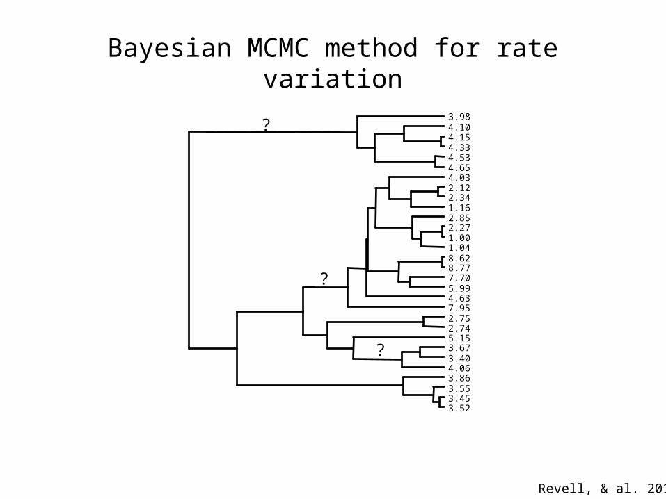
Bayesian MCMC method for rate variation
3.523.453.553.864.063.403.675.152.742.757.954.635.997.708.778.621.041.002.272.851.162.342.124.034.654.534.334.154.103.98
?
?
?
Revell, & al. 2012

Bayesian MCMC chain: evol.rate.mcmc()
posterior sample
Startingvalues
σ12 σ2
2
Evolutionary rates & rate-
shift
Proposalσ1
2 σ22
Propose new rate-shift (or
rates)
σ12 σ2
2σ12σ12 σ2
2σ22 σ1
2σ12 σ2
2σ22
σ12σ12 σ2
2σ22
÷÷÷÷÷
ø
ö
ççççç
è
æ
÷÷ø
öççè
æ÷÷ø
öççè
æ
÷÷ø
öççè
æ÷÷ø
öççè
æ
=XLP
XLP
|
|
,1mina
σ12 σ2
2σ12σ12 σ2
2σ22
σ12σ12 σ2
2σ22
σ12 σ2
2σ12σ12 σ2
2σ22
Compute posterior odds ratio
σ12 σ2
2σ12σ12 σ2
2σ22
)1,0(~Urif
Retain proposal with probability α
Repeat
σ12σ12 σ2
2σ22
)1,0(~Urif
Reject proposal with probability 1-α

posterior sample
Startingvalues
σ12 σ2
2
Evolutionary rates & rate-
shift
Startingvalues
σ12σ12 σ2
2σ22
Evolutionary rates & rate-
shift
Proposalσ1
2 σ22
Propose new rate-shift (or
rates)
Proposalσ1
2σ12 σ2
2σ22
Propose new rate-shift (or
rates)
σ12 σ2
2σ12σ12 σ2
2σ22 σ1
2σ12 σ2
2σ22σ1
2σ12 σ2
2σ22
σ12σ12 σ2
2σ22
XLP
XLP
|
|
,1min
σ12 σ2
2σ12σ12 σ2
2σ22
σ12σ12 σ2
2σ22
σ12 σ2
2σ12σ12 σ2
2σ22
Compute posterior odds ratio
σ12σ12 σ2
2σ22
XLP
XLP
|
|
,1min
σ12 σ2
2σ12σ12 σ2
2σ22
σ12σ12 σ2
2σ22
σ12 σ2
2σ12σ12 σ2
2σ22
Compute posterior odds ratio
σ12 σ2
2σ12σ12 σ2
2σ22
)1,0(~Urif
Retain proposal with probability α
σ12 σ2
2σ12σ12 σ2
2σ22
)1,0(~Urif
Retain proposal with probability α
Repeat
σ12σ12 σ2
2σ22
)1,0(~Urif
Reject proposal with probability 1-α
σ12σ12 σ2
2σ22
)1,0(~Urif
Reject proposal with probability 1-α
Bayesian MCMC chain

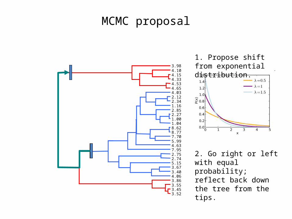
MCMC proposal
3.523.453.553.864.063.403.675.152.742.757.954.635.997.708.778.621.041.002.272.851.162.342.124.034.654.534.334.154.103.98
σ22
σ12
Rate shift point with two evolutionary rates: the rate tipward (σ2
2, in this case) and rootward of the rate-shift.
3.523.453.553.864.063.403.675.152.742.757.954.635.997.708.778.621.041.002.272.851.162.342.124.034.654.534.334.154.103.98
MCMC proposal
1. Propose shift from exponential distribution.
2. Go right or left with equal probability; reflect back down the tree from the tips.

MCMC proposal
3.523.453.553.864.063.403.675.152.742.757.954.635.997.708.778.621.041.002.272.851.162.342.124.034.654.534.334.154.103.98
σ12
σ22
1. Propose shift from exponential distribution.
2. Go right or left with equal probability; reflect back down the tree from the tips.

Averaging the posterior sample: min.split()
To find the median shift-point in our sample, we first computed the patristic distance between all the shifts in our posterior sample.
We then picked the split with the lowest summed distance to all the other sample.
(We might have instead found the shift with the lowest sum of squared distances, or found a point on a tree that minimized the sum of squared distances.)

Averaging the posterior sample: min.split()
We can also compute the posterior probabilities of the shift being on any edge.
We just calculate these as the frequency of the edge in the posterior sample.
0.97
0.01
0.02
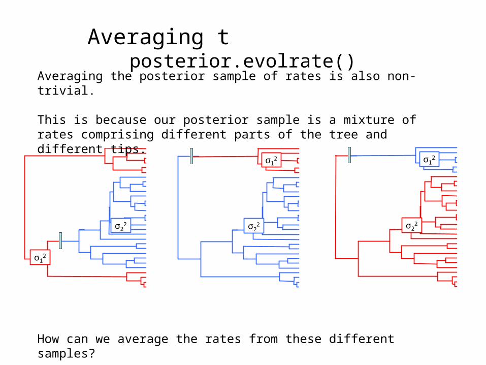
Averaging the posterior: posterior.evolrate()
σ22
σ12
σ12
σ22
σ12
σ22
Averaging the posterior sample of rates is also non-trivial.
This is because our posterior sample is a mixture of rates comprising different parts of the tree and different tips.
How can we average the rates from these different samples?
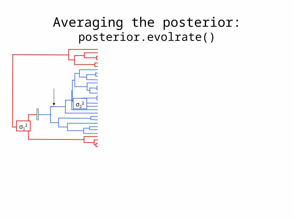
Averaging the posterior: posterior.evolrate()
σ22
σ12

Averaging the posterior: posterior.evolrate()
σ22
σ12
X X

Averaging the posterior: posterior.evolrate()
X X
x σ12
x σ22

Averaging the posterior: posterior.evolrate()

Averaging the posterior: posterior.evolrate()
X
X
x σ22
x σ12
In this case, σ22 = σ2
2;
while σ12 > σ1
2

Identification of the “correct” edge
Somewhat surprisingly, identification of the “correct” edge was effectively independent of the number of tips in the tree for a given rate shift.
However, relative patristic distance from the true shift point does decline with increasing N.

Estimating the evolutionary rates
We do get better at estimating the evolutionary rates unbiasedly (and their ratio) for increased N.
The evolutionary rates tend to be biased towards each other for small N, which we think is a natural consequence of integrating over uncertainty in the location of the rate shift.

Outline
1. The ‘phytools’ package.2. New approaches for the analysis of
quantitative trait data:a) Phylogenetic analysis of the evolutionary
correlation.b) Bayesian method for locating rate shifts in the
tree.c) Incorporating intraspecific variability in
phylogenetic analyses.
3. Luke!

• Phylogenetic comparative analyses are conducted with species means.
• But data in empirical studies are uncertain estimates obtained by measuring one or a few individuals.
• **Ignoring intraspecific variability can cause bias in various types of comparative analysis.
• Our solution: sample both species means & variances, and the parameters of the evolutionary model, from their joint posterior distribution using Bayesian MCMC.
Introduction
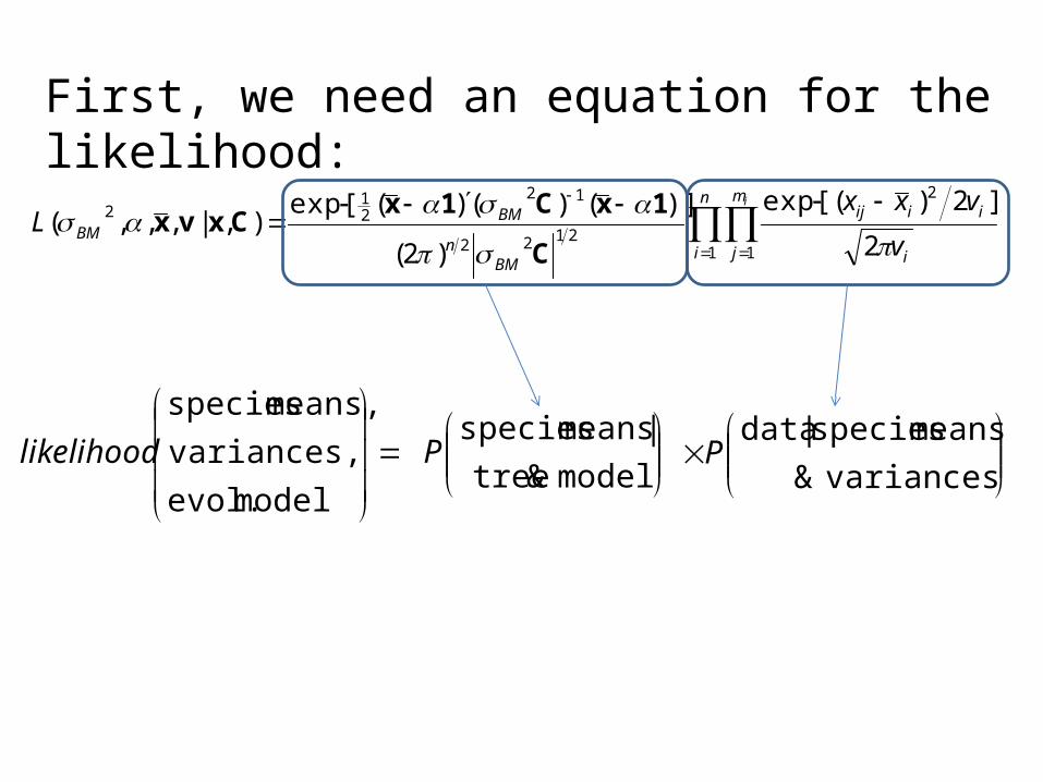
First, we need an equation for the likelihood:
n
i
m
j i
iiij
BMn
BMBM
i
v
vxxL
1 1
2
2122
1221
2
2
]2)(exp[
)2(
)]()()(exp[),|,,,(
C
1xC1xCxvx
model & tree
| means speciesP
variances &
means species | dataP
model evol.
variances,
means, species
likelihood

-0.3530.906
0.552,0.371,1.155,0.483-0.329,0.521,-0.013,-1.08
-2.322,-1.809
-0.707
1.31
-1.444,-0.889-1.277,-0.545
-1.246,-0.335,-0.086-0.583
0.218,0.721,1.144,0.4982.547,2.071
-0.8,-1.111
-0.346
-1.292-1.381,-1.547
0.621,0.795,0.065,0.697
0.172,-0.303,0.137-0.264,-0.005
-0.783,0.101,-0.7390.376,-0.278,-0.094,0.667
2.6582.683,2.656
0.679,-0.288,-0.404-0.456
3.249,2.157,2.845,2.2992.596,3.375,3.843
-0.275,0.179,-0.605,-0.206-0.269,0.373
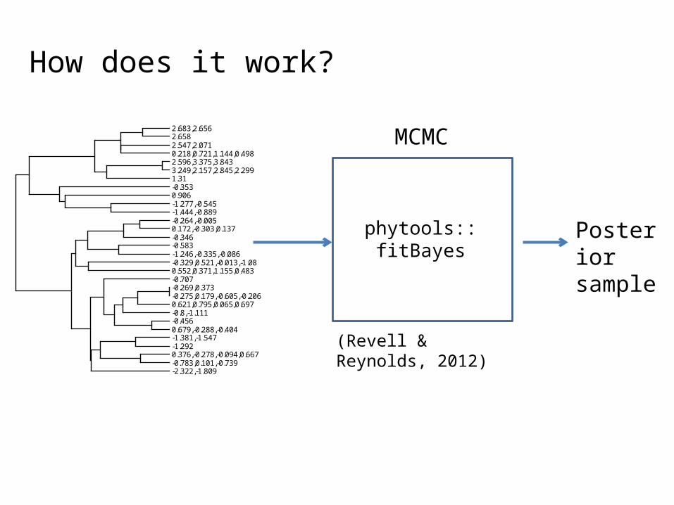
How does it work?
-0.3530.906
0.552,0.371,1.155,0.483-0.329,0.521,-0.013,-1.08
-2.322,-1.809
-0.707
1.31
-1.444,-0.889-1.277,-0.545
-1.246,-0.335,-0.086-0.583
0.218,0.721,1.144,0.4982.547,2.071
-0.8,-1.111
-0.346
-1.292-1.381,-1.547
0.621,0.795,0.065,0.697
0.172,-0.303,0.137-0.264,-0.005
-0.783,0.101,-0.7390.376,-0.278,-0.094,0.667
2.6582.683,2.656
0.679,-0.288,-0.404-0.456
3.249,2.157,2.845,2.2992.596,3.375,3.843
-0.275,0.179,-0.605,-0.206-0.269,0.373
MCMC
phytools::fitBayes
Posterior sample
(Revell & Reynolds, 2012)
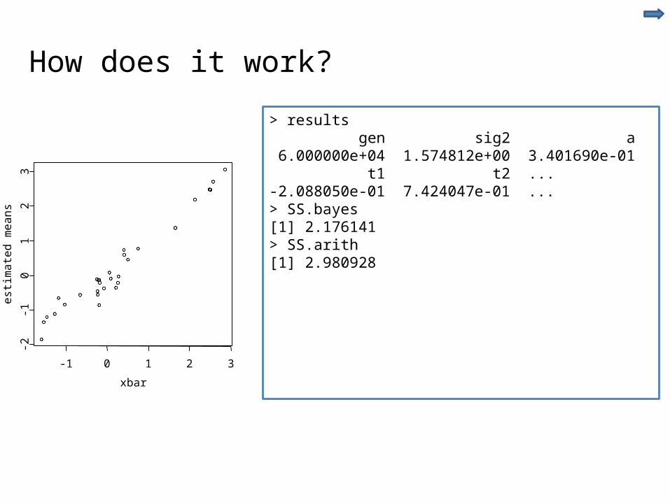
How does it work?

> results gen sig2 a 6.000000e+04 1.574812e+00 3.401690e-01 t1 t2 ... -2.088050e-01 7.424047e-01 ...-0.353
0.906
0.552,0.371,1.155,0.483-0.329,0.521,-0.013,-1.08
-2.322,-1.809
-0.707
1.31
-1.444,-0.889-1.277,-0.545
-1.246,-0.335,-0.086-0.583
0.218,0.721,1.144,0.4982.547,2.071
-0.8,-1.111
-0.346
-1.292-1.381,-1.547
0.621,0.795,0.065,0.697
0.172,-0.303,0.137-0.264,-0.005
-0.783,0.101,-0.7390.376,-0.278,-0.094,0.667
2.6582.683,2.656
0.679,-0.288,-0.404-0.456
3.249,2.157,2.845,2.2992.596,3.375,3.843
-0.275,0.179,-0.605,-0.206-0.269,0.373
How does it work?

-1 0 1 2 3
-2-1
01
23
xbar
est
ima
ted
me
an
s
How does it work?
-1 0 1 2 3
-2-1
01
23
xbar
est
ima
ted
me
an
s
> results gen sig2 a 6.000000e+04 1.574812e+00 3.401690e-01 t1 t2 ... -2.088050e-01 7.424047e-01 ...> SS.bayes[1] 2.176141> SS.arith[1] 2.980928
How does it work?

Is this result general . . . . YES!
Generating σ2
0.2
0.0
0.2
0.3
Mea
n sq
uare
err
or-- MSE Bayesian means-- MSE arithmetic means
0.4
0.1
0.4 0.6 0.8 1.0

Outline
1. The ‘phytools’ package.2. New approaches for the analysis of
quantitative trait data:a) Phylogenetic analysis of the evolutionary
correlation.b) Bayesian method for locating rate shifts in the
tree.c) Incorporating intraspecific variability in
phylogenetic analyses.
3. Luke!
Related Documents