NEW ORTHOGONAL SPACE-TIME BLOCK CODES WITH FULL DIVERSITY A Thesis by LORI ANNE DALTON Submitted to the Office of Graduate Studies of Texas A&M University in partial fulfillment of the requirements for the degree of MASTER OF SCIENCE December 2002 Major Subject: Electrical Engineering

Welcome message from author
This document is posted to help you gain knowledge. Please leave a comment to let me know what you think about it! Share it to your friends and learn new things together.
Transcript

NEW ORTHOGONAL SPACE-TIME BLOCK CODES WITH FULL DIVERSITY
A Thesis
by
LORI ANNE DALTON
Submitted to the Office of Graduate Studies ofTexas A&M University
in partial fulfillment of the requirements for the degree of
MASTER OF SCIENCE
December 2002
Major Subject: Electrical Engineering

NEW ORTHOGONAL SPACE-TIME BLOCK CODES WITH FULL DIVERSITY
A Thesis
by
LORI ANNE DALTON
Submitted to Texas A&M Universityin partial fulfillment of the requirements
for the degree of
MASTER OF SCIENCE
Approved as to style and content by:
Costas N. Georghiades(Chair of Committee)
Scott L. Miller(Member)
Chin B. Su(Member)
Marina Vannucci(Member)
Chanan Singh(Head of Department)
December 2002
Major Subject: Electrical Engineering

iii
ABSTRACT
New Orthogonal Space-Time Block Codes with Full Diversity. (December 2002)
Lori Anne Dalton, B.S., Texas A&M University
Chair of Advisory Committee: Dr. Costas N. Georghiades
It has been shown from the Hurwitz-Radon theorem that square complex orthog-
onal space-time code designs cannot achieve full diversity and full rate simultaneously,
except in the two transmit antenna case. However, this result does not consider non-
linear codes, or codes that only exist for specific symbol constellation sets. In this
work, we present complex full rate codes for four transmit antennas. Using carefully
tailored constellation phase rotations, we show these codes can achieve full diversity
for specialized PSK and PAM symbol constellations. In addition, one code presented
with PAM based symbols is a linear complex orthogonal design. Thus, we demon-
strate by example that full rate, full diversity, square complex orthogonal codes for
four transmit antennas exist when symbol constellations are restricted to a subset
of the complex plane. This new code does not violate the Hurwitz-Radon theorem,
which only considers codes that work for all possible symbol constellations.

iv
To my wonderful parents, Scott and Tahnee, and my terrific little brother, Maxim

v
ACKNOWLEDGMENTS
I would first like to thank my advisor, Dr. Costas Georghiades, for introducing
me to wireless communications and space-time coding. He has been an excellent guide
in my transition from undergraduate school to graduate school. I also thank my other
committee members, Dr. Scott Miller, Dr. Chin Su, and Dr. Marina Vannucci, for
their valuable comments and for committing their time to help me with this work.
Thanks also to the remaining professors of the wireless communications group: Dr.
Krishna Narayanan, Dr. Zixiang Xiong, Dr. Erchin Serpedin, and Dr. Xiaodong
Wang (now at Columbia University), for their input and support.
I could not be where I am today without the unconditional love and encourage-
ment of my parents and brother. I thank my Mom and brother particularly for their
emotional and spiritual support. Without them, my life would not be complete. Fi-
nally, I thank my Dad for continually stimulating my mind and inspiring my interest
in engineering, math, and science. I remember fondly my very first lesson on numbers
from him.

vi
TABLE OF CONTENTS
CHAPTER Page
I INTRODUCTION . . . . . . . . . . . . . . . . . . . . . . . . . . 1
A. Introduction to the Wireless Problem . . . . . . . . . . . . 1
B. Introduction to Space-Time Coding . . . . . . . . . . . . . 2
1. Notation . . . . . . . . . . . . . . . . . . . . . . . . . 3
2. Channel Model . . . . . . . . . . . . . . . . . . . . . . 4
3. The Code Matrix . . . . . . . . . . . . . . . . . . . . 5
C. Benefits of Space-Time Coding . . . . . . . . . . . . . . . . 5
1. Improved Performance with Diversity . . . . . . . . . 5
2. Higher Data Rate, Capacity, and Spectral Efficiency . 7
3. Simpler Handheld Design . . . . . . . . . . . . . . . . 9
D. Orthogonal Code Matrix Design . . . . . . . . . . . . . . . 9
E. Literature Review . . . . . . . . . . . . . . . . . . . . . . . 13
II A CLASS I NON-LINEAR ORTHOGONAL CODE . . . . . . . 15
A. An Example: The Alamouti Code . . . . . . . . . . . . . . 15
B. An Example: STTD-OTD . . . . . . . . . . . . . . . . . . 16
C. The New Code Matrix . . . . . . . . . . . . . . . . . . . . 18
D. Linearity . . . . . . . . . . . . . . . . . . . . . . . . . . . . 19
E. Diversity Analysis . . . . . . . . . . . . . . . . . . . . . . . 19
III A CLASS II NON-LINEAR ORTHOGONAL CODE . . . . . . 21
A. The New Code Matrix . . . . . . . . . . . . . . . . . . . . 22
B. Linearity . . . . . . . . . . . . . . . . . . . . . . . . . . . . 24
C. Diversity Analysis . . . . . . . . . . . . . . . . . . . . . . . 25
D. Constellation Design . . . . . . . . . . . . . . . . . . . . . 26
1. PAM Based Constellations . . . . . . . . . . . . . . . 26
2. PSK Based Constellations . . . . . . . . . . . . . . . . 27
E. Capacity . . . . . . . . . . . . . . . . . . . . . . . . . . . . 28

vii
CHAPTER Page
F. Receivers for Known Fading . . . . . . . . . . . . . . . . . 31
1. Optimal Receivers . . . . . . . . . . . . . . . . . . . . 31
a. Using PAM Base Constellations . . . . . . . . . . 34
b. Using PSK Base Constellations . . . . . . . . . . 35
2. Sub-Optimal Receivers . . . . . . . . . . . . . . . . . 35
G. Receivers for Unknown Known Fading . . . . . . . . . . . 36
IV PERFORMANCE . . . . . . . . . . . . . . . . . . . . . . . . . . 39
A. Class I Non-Linear Code Performance . . . . . . . . . . . . 40
1. Non-Rotated QPSK Constellations . . . . . . . . . . . 40
2. Rotated QPSK Constellations . . . . . . . . . . . . . . 41
B. Class II Non-linear Code Performance . . . . . . . . . . . . 42
1. Rotated 4-PAM Constellations . . . . . . . . . . . . . 42
2. Rotated QPSK Constellations and Linear Receiver . . 43
3. Rotated QPSK Constellations and ML Receiver . . . . 44
4. Rotated BPSK Constellations and Unknown Fading . 45
V CONCLUSION . . . . . . . . . . . . . . . . . . . . . . . . . . . 47
A. Summary of Results . . . . . . . . . . . . . . . . . . . . . 47
B. Future Work . . . . . . . . . . . . . . . . . . . . . . . . . . 48
REFERENCES . . . . . . . . . . . . . . . . . . . . . . . . . . . . . . . . . . . 49
APPENDIX A . . . . . . . . . . . . . . . . . . . . . . . . . . . . . . . . . . . 53
VITA . . . . . . . . . . . . . . . . . . . . . . . . . . . . . . . . . . . . . . . . 56

viii
LIST OF TABLES
TABLE Page
I “Bad” matrices for the class I non-linear code with QPSK sym-
bols, phase shifted by [0, 1, 2, 3] π/16. . . . . . . . . . . . . . . . . . . 54

ix
LIST OF FIGURES
FIGURE Page
1 A typical communication system utilizing space-time coding. . . . . . 3
2 Capacity of various (Nt, Nr = Nt) systems. . . . . . . . . . . . . . . 8
3 (a) Constellations for PAM base symbols; (b) Resulting QAM
transmit constellation. . . . . . . . . . . . . . . . . . . . . . . . . . 27
4 (a) Constellations for QPSK base symbols; (b) Resulting transmit
constellation. . . . . . . . . . . . . . . . . . . . . . . . . . . . . . . . 29
5 Diversity product of the class II non-linear code with QPSK base
symbols; d2 and d4 are rotated by φ with respect to d1 and d3. . . . . 30
6 Capacity of the class II non-linear orthogonal code. . . . . . . . . . . 32
7 ML performance of the class I non-linear code with QPSK base
symbols and no phase shifts. . . . . . . . . . . . . . . . . . . . . . . . 40
8 ML performance of the class I non-linear code with QPSK symbols
and phase shifts [0, 0, 32, 19] π/128. . . . . . . . . . . . . . . . . . . . 41
9 ML performance of the orthogonal code with 4PAM base symbols
and phase shifts [0, 1, 0, 1] π/2. . . . . . . . . . . . . . . . . . . . . . . 42
10 ZF and linear MMSE performance of the class II non-linear code
with QPSK base symbols and phase shifts [0, 1, 0, 1] π/4. . . . . . . . 43
11 ML performance of the class II non-linear code with QPSK base
symbols and phase shifts [0, 1, 0, 1] π/4. . . . . . . . . . . . . . . . . . 44
12 Sub-optimal performance in unknown fading (fmT = 0) of the
class II non-linear code with BPSK base symbols and phase shifts
[0, 1, 0, 1] π/2. . . . . . . . . . . . . . . . . . . . . . . . . . . . . . . . 46
13 QPSK symbol constellations with phase shifts [0, 1, 2, 3] π/16. . . . . 55

1
CHAPTER I
INTRODUCTION
We first describe the wireless problem in Section A and present an introduction to
space-time coding in Section B. In Section C, benefits of space-time coding are
covered, followed by a discussion on orthogonal code design in Section D. In the latter
section, we define two classes of “non-linear” orthogonal codes. Finally, a review of
literature relevant to space-time block code design is presented in Section E.
A. Introduction to the Wireless Problem
Due to an explosion of demand for high-speed wireless services, such as wireless In-
ternet, email, stock quotes, and cellular video conferencing, wireless communications
has become one of the most exciting fields in modern engineering. However, devel-
opment of such products and services poses a serious challenge: how can we support
the exceedingly high data rates and capacity required for these applications with the
severely restricted resources offered in a wireless channel?
The obstacles associated with wireless environments are difficult to overcome.
Interference from other users and inter-symbol interference (ISI) from multiple paths
of one’s own signal are serious forms of distortion [1], the latter effectively causing
frequency-selective channel properties. Furthermore, when transmit and receive an-
tennas are in relative motion, the Doppler effect will spread the frequency spectrum
of received signals [2]. This results in time varying channel characteristics. Many sys-
tems must function without a line-of-sight (LOS) path between transmit and receive
antennas, thus pure Rayleigh fading may completely attenuate a signal at times and
The journal model is IEEE Transactions on Automatic Control.

2
render a channel temporarily useless. Additionally, the usual additive white Gaussian
noise (AWGN) corrupts the signal.
Besides the above difficulties, there are extremely limited bandwidth and strin-
gent power limitations on both the mobile unit (for battery conservation) and the
base station (to satisfy government safety regulations). To conserve bandwidth re-
sources, we maximize spectral efficiency by packing as much information as possible
into a given bandwidth. A solution to the bandwidth and power problem is the cel-
lular concept, in which frequency bands are allocated to small, low power cells and
reused at cells far away. However, this idea alone is not enough. We must look to
other means, such as space-time coding, to increase data rate, capacity, and spectral
efficiency.
B. Introduction to Space-Time Coding
A typical communication system consists of a transmitter, a channel, and a receiver.
Space-time coding involves use of multiple transmit and receive antennas, as illus-
trated in Fig. 1. Bits entering the space-time encoder serially are distributed to
parallel sub-streams. Within each sub-stream, bits are mapped to signal waveforms,
which are then emitted from the antenna corresponding to that sub-stream. The
scheme used to map bits to signals is the called a space-time code. Signals trans-
mitted simultaneously over each antenna interfere with each other as they propagate
through the wireless channel. Meanwhile, the fading channel also distorts the signal
waveforms. At the receiver, the distorted and superimposed waveforms detected by
each receive antenna are used to estimate the original data bits.

3
Space-TimeEncoder
Data In
Space-TimeDecoder
Data Out
1
2
1
2r1
r2
h11
h21
h22
h12
FadingChannel
TransmitAntenna
Array
ReceiveAntenna
Array
Fig. 1. A typical communication system utilizing space-time coding.
1. Notation
The following notation is used throughout this thesis.
• j =√−1.
• x∗ is the complex conjugate of x.
• < (x) is the real part of x.
• ∠x is the phase of x.
• E [X] is the expected value of random variable X.
• XT is the transpose of matrix X.
• XH is the conjugate transpose of matrix X.
• In is the n× n identity matrix.
• 0n is the n× n zero matrix.

4
2. Channel Model
In a space-time system, define Nt to be the number transmit antennas and Nr the
number of receive antennas. Furthermore, assume we use a block coded system in
which L2M bits enter the encoder every block epoch. These bits are mapped to L
symbols, each with an M -ary sized constellation, and transmitted over a block of T
time intervals. We say this is an (Nt, Nr) block coded system with rate R = L/T . A
mathematical model for any space-time block coded system is given by
R = S ·H + N, (1.1)
where
• R is a T ×Nr matrix representing the received data.
• S is a T ×Nt matrix representing the transmitted symbols.
• H is an Nt ×Nr matrix representing quasi-static flat Gaussian fading.
• N is a T ×Nr matrix representing AWGN.
In the channel model (1.1), we only consider fading and AWGN distortion. El-
ements of the AWGN matrix, N, are modeled as independent circularly symmetric
(i.e., real and imaginary parts are independent) complex Gaussian random variables
with zero mean, and a variance that defines the system signal-to-noise ratio (SNR).
The fading matrix, H, is modeled in the same statistical manner as AWGN with
normalized unit variance [1], [2]. A quasi-static channel remains constant over the
duration of a code block, but changes independently from one block to another. Flat
fading implies a constant power spectral density (PSD) over the frequency band used
by the transmitted symbols [2]. We assume all antennas in the system are placed
sufficiently far apart for independent fading over each channel.

5
3. The Code Matrix
Elements of code matrix S are typically complex baseband symbols from a PSK or
QAM constellation. A given column of S represents the stream of data sent by a
specific transmit antenna, while a given row represents the information sent in a
single time interval. This structure in the code matrix gives the name, “space-time
coding.” The average energy transmitted in each space-time code block satisfies
E[trace
(SSH
)]= TNtE, where E is the average complex baseband symbol energy.
C. Benefits of Space-Time Coding
1. Improved Performance with Diversity
Space-time coding can improve performance through an effect known as diversity.
Diversity is a measure of the average number of channels fully utilized by each piece
of information transmitted. The maximum diversity available to a space-time system
is NtNr, which is the total number of channels between the transmitter and receiver.
When adding new antennas to a system, the receiver can use the extra channels
to improve the probability of correctly identifying the true transmitted signal. We
may view the new channels as redundancy, or backup in case other channels fail.
For example, suppose we have one transmit and two receive antennas, and that one
of the channels goes into a deep fade and is basically unusable. In this case, the
other channel may still be able to recover the data. While both channels might
fail simultaneously, this is highly unlikely compared to the event of a single channel
failure. This is demonstrated by the following property of independent events.
Pr (“channel 1 fails” and “channel 2 fails”)
= Pr (“channel 1 fails”) Pr (“channel 2 fails”) .

6
In this way, space-time coding offers the possibility of lower error probability.
Diversity in a fading channel can be directly determined from error probability.
Specifically, the diversity of a system is given by the error probability behavior as
SNR →∞, i.e.,
Pr (error) = Kρ−D,
where D is the diversity order, ρ is the SNR, and K is a coding gain constant. Thus,
performance plots on a log scale with SNR in dB approach a linear asymptote with
slope −D.
In [4], the rank criterion was developed to determine the diversity order achieved
by space-time codes. Essentially, it states D = NNr, where N is the minimum rank
of the difference between any two distinct code matrices, S − S. For a full diversity
code, N = Nt. A necessary, but insufficient, condition for full diversity is that each
symbol must be transmitted over every antenna. Another performance criterion is
the determinant criterion, which addresses coding gain. For full diversity schemes, it
simply maximizes the minimum determinant of S− S.
For square code matrices, one measure of the quality of a space-time code is the
diversity product [5], given by
ζv =1
2min
S 6=eS∈V
∣∣∣det(S− S
)∣∣∣1
Nt , (1.2)
where V is the set of all data matrices S. We observe ζv is a measure of minimum
distance. Some properties of the diversity product are listed below.
• 0 ≤ ζv ≤√
NtE.
• Any constellation with ζv > 0 achieves full diversity (from the rank criterion).
• Larger ζv typically indicates a better code (from the determinant criterion).

7
2. Higher Data Rate, Capacity, and Spectral Efficiency
In general, the data rate of a space-time block code is defined to be the average
number of symbols sent per time epoch, or simply R = L/T . A space-time code is
full rate if L = T . The spectral efficiency of a modulation scheme is given by
η =Data Rate
Bandwidth.
We define the spectral efficiency of a space-time code using a two-dimensional con-
stellation with M points to be η = R log2 M bits/sec/Hz.
Improved performance from diversity may be used to attain higher data rates
by increasing the symbol constellation size. Since M -PSK and M -QAM modulations
are bandwidth efficient signaling schemes (they use a fixed amount of bandwidth for
any M), space-time coding enables us to achieve higher levels of spectral efficiency at
a fixed bandwidth and error rate.
It has been shown in [6] and [7] that space-time codes can achieve phenomenal
capacity compared to traditional single transmit and receive antenna systems. In
general, the capacity of a multi-input multi-output (MIMO) channel with Gaussian
fading is
C = EH
[log det
(INr +
ρ
Nt
HHH
)](1.3)
= EH
[log det
(INt +
ρ
Nt
HHH
)], (1.4)
where ρ is the SNR. A plot of capacity is illustrated in Fig. 2 for various systems
with Nr = Nt receive antennas. Notice as the number of antennas is increased that
capacity increases significantly. BLAST [8] is a space-time coding technique designed
to achieve capacity and maximize data rate.

8
0 5 10 15 20 25 30 350
10
20
30
40
50
60
70
80
90
SNR (dB)
Cap
acity
(bi
ts)
(1, 1)(2, 2)(4, 4)(8, 8)
Fig. 2. Capacity of various (Nt, Nr = Nt) systems.

9
3. Simpler Handheld Design
We can achieve the same diversity effects with multiple antennas at the transmitter
as with multiple antennas at the receiver. Thus, transmit diversity is appealing in
systems with multiple information recipients, such as broadcast and cellular schemes.
This is because we can increase diversity in all subscriber units by adding just one
antenna to the base station, instead of a new antenna to each individual receiving
unit, thus reducing the cost and complexity of each handheld device.
D. Orthogonal Code Matrix Design
Currently, there is interest in designing codes for 4 or more transmit antennas. Most
space-time block codes in the literature are motivated by one or more of the follow-
ing desirable properties: full diversity, full rate, simple maximum-likelihood (ML)
detection, and minimum delay (i.e., a square code matrix).
Orthogonal codes are most remarkable for having simple ML receivers that de-
couple the symbols. In [3], several classes of full diversity orthogonal designs were
defined. All of these codes (listed below) require SHS = DNt1, where DNt is a di-
agonal matrix whose diagonal elements are real linear combinations of the symbol
energies, |si|2, i = 1, . . . , L.2
• Real orthogonal designs: an Nt×Nt matrix with real entries ±si, i = 1, . . . , Nt.
• Complex orthogonal designs: an Nt×Nt matrix with complex entries ±si, ±s∗i ,
±jsi, and ±js∗i , i = 1, . . . , Nt.
1This condition essentially requires the symbol streams transmitted by each an-tenna to be orthogonal to each other. Note for real designs SHS = STS.
2An orthogonal code has full diversity if these linear combination coefficients arestrictly positive.

10
• Real linear processing orthogonal designs: an Nt × Nt matrix with real linear
combinations of si, i = 1, . . . , Nt, as entries.
• Complex linear processing orthogonal designs: an Nt×Nt matrix with complex
linear combinations of si and s∗i , i = 1, . . . , Nt, as entries.
• Generalized real orthogonal designs: a T × Nt matrix with entries 0 or ±si,
i = 1, . . . , L.
• Generalized complex orthogonal designs: a T × Nt matrix with entries 0, ±si,
±s∗i , ±jsi, and ±js∗i , i = 1, . . . , L.
It was shown in [3] that full diversity orthogonal designs exist if and only if a
code exists such such that
SHS =T
L
(|s1|2 + |s2|2 + · · ·+ |sL|2)INt . (1.5)
For an orthogonal code satisfying (1.5) with equal energy symbols, S is a scaled
unitary matrix, i.e., SHS = TEINt . For a square code matrix (T = Nt), the criterion
SHS = TEINt is equivalent to SSH = TEIT . However, for T > Nt, the ranks of SHS
and SSH should be the same, and thus SSH = TEIT does not hold. For T < Nt,
SHS = TEINt is not possible.
Consider code matrices containing only linear combinations of the data symbols.
We may set the ith column of S to BiXT , where X is a row vector of the L = T
real symbols transmitted in a block, and the Bi are arbitrary L × L real matrices.
To construct generalized (T ≥ Nt) full rate, full diversity real orthogonal designs, Bi
must satisfy,
BiBTi = BT
i Bi = IL, 1 ≤ i ≤ Nt, (1.6)
BTi Bj = −BT
j Bi, 1 ≤ i, j ≤ Nt. (1.7)

11
Let Aj = BT1 Bj, for j = 1, . . . , Nt (note A1 = INt). Then the criteria (1.6) and (1.7)
become:
ATi Ai = IL, 2 ≤ i ≤ Nt, (1.8)
ATi = −Ai, 2 ≤ i ≤ Nt, (1.9)
AiAj = −AjAi, 2 ≤ i, j ≤ Nt. (1.10)
These conditions define a size Nt − 1 family of L × L Hurwitz-Radon matrices. It
was shown in [3] that a size k Hurwitz-Radon family of n × n matrices is limited in
size by k ≤ n − 1, and that equality is only possible for n = 2, 4, or 8. Applying
this mathematical result to orthogonal designs, we discover that real full rate and full
diversity square orthogonal designs (Nt = L = T ) only exist for Nt = 2, 4, or 8.
Define A (R, Nt) to be the minimum T such that a T ×Nt real orthogonal code
matrix exists with at least rate R. For full rate codes (R = 1), this is equivalent
to the minimum T such that a size Nt − 1 family of T × T Hurwitz-Radon matrices
exists. It was shown in [3] that A (R, Nt) is finite for any R, and for full rate codes,
A (1, Nt) = min0≤c, 0≤d<4, 8c+2d≥Nt
24c+d.
Delay optimal real orthogonal codes (codes that achieve minimum T ) with full rate
and full diversity are not square codes unless Nt = 2, 4, or 8, but they do exist for
all Nt. For example, we can construct codes for Nt = 7 by deleting any column of an
Nt = 8 code.
For complex designs, a similar analysis shows that full rate and full diversity
square orthogonal codes only exist for 2 transmit antennas. Given a complex orthog-
onal design of size Nt, Replace each symbol si = si,r + si,qj in the code matrix with

12
a 2× 2 matrix,
si,r si,q
−si,q si,r
.
The new code matrix formed is a real orthogonal design of size 2Nt. Define Ac (R, Nt)
to be the minimum T such that a T ×Nt complex orthogonal code matrix exists with
at least rate R. For any R ≤ 0.5, Ac (R,Nt) is finite. In general for all R,
Ac (R, Nt) ≥ 1
2A (R, 2Nt) .
Delay optimal complex orthogonal codes with full rate and full diversity are not square
codes unless Nt = 2, but they might exist for Nt > 2. Rate 1/2 codes are known
to exist for all Nt, and only sporadic codes for R = 3/4 are known for Nt = 3 and
Nt = 4.
Notice both real and complex orthogonal designs only consider linear codes de-
signed to work for all possible symbol constellations. At this point, we define two
classes of complex “non-linear” orthogonal codes:
• Class I designs: a T ×Nt matrix with linear or non-linear functions of si and s∗i ,
i = 1, . . . , L, as entries. The matrix must satisfy SHS = DNt , where DNt is a
diagonal matrix whose diagonal elements are linear combinations of the symbol
energies.
• Class II designs: a T × Nt matrix with linear combinations of si and s∗i , i =
1, . . . , L, as entries. The matrix must satisfy SHS = DNt , where DNt is a
diagonal matrix whose diagonal entries are linear or non-linear functions of the
symbol energies.
These definitions do not guarantee full diversity or linear processing at the receiver,
but allow more flexibility in designing codes. Note orthogonal codes are a special case
13
of non-linear orthogonal codes.
E. Literature Review
Delay diversity [9], [10] and other related schemes [11], [12] were among the first
techniques presented to exploit transmit diversity. Delay diversity can be viewed
as a special case of space-time trellis coding (STTC), later developed by Tarokh
et.al. [4]. The generalized approach combines trellis coded modulation (TCM) with
transmit diversity techniques, and though decoding complexity for these codes grows
exponentially with the number of antennas, they perform very well in slowly fading
environments. The rank and determinant criteria emerged from this work and be-
came a benchmark in space-time code design. A more structured method of STTC
construction ensuring full diversity was later presented in [13].
The Alamouti code [14], remarkable for having an elegant and simple linear re-
ceiver, became a paradigm in space-time block coding (STBC). Alamouti’s idea for
two transmit antennas was generalized by orthogonal designs [3], [15], which have full
diversity and linear maximum likelihood (ML) detectors that decouple the transmit-
ted symbols. Unfortunately, the Hurwitz-Radon theorem showed that square complex
linear processing orthogonal designs cannot achieve full diversity and full rate simulta-
neously, except in the two transmit antenna case [3], [16] (a formula for the maximum
achievable data rate for square code matrices was given in [17]). For 3 or 4 transmit
antennas, several orthogonal codes have been discovered with full diversity and a rate
of 3/4 [3], [15]–[18]. As shown in [19], though, it is possible to design orthogonal, full
rate and full diversity complex codes for more than two transmit antennas for specific
signal constellations.
Similarly to orthogonal codes, unitary space-time modulation [20] and differential

14
unitary modulation [5] use a set of unitary code matrices to represent data. In
general, the optimal receiver for a unitary modulation code is more complex than for
an orthogonal design because the code matrix is not structured by symbols that can
be decoupled for detection. These codes are typically non-square and designed for
systems where channel state information (CSI) is unknown at the receiver.
The ABBA code presented in [21] and similar codes [22]–[24] have full rate,
but are quasi-orthogonal3 and offer a diversity order of only 2. The STTD-OTD
code [25] provides some diversity gain by grouping symbols into Alamouti blocks and
transforming them using a Walsh-Hadamard matrix. For the 4 transmit antenna
case, this orthogonal code has full rate and diversity order 2. Recently, an orthogonal
full diversity, full rate STBC for 4 transmit antennas was presented in [30]. However
perfect knowledge of the channel at the transmitter and receiver is required to cancel
inter-symbol-interference (ISI) and ensure orthogonality.
It has been shown that full diversity and full rate can be achieved with gen-
eralized algebraic space-time (GAST) codes, which use rotated constellations with
a Hadamard transform [26]. In addition, these non-orthogonal codes offer a coding
gain over comparable orthogonal codes, especially for large constellations and many
transmit antennas. Another code in the literature utilizes space-time diversity with
unitary constellation rotating precoders [27]–[29]. Constellation rotating codes es-
sentially transmit a linear combination of the phase-rotated symbols through one
antenna at a time, while leaving the other antennas silent. These codes are distinct
for achieving full rate and full diversity, but are not orthogonal.
3Define Zi to be the ith column of the code matrix S, i = 1, . . . , Nt. A code isquasi-orthogonal if the Zi can be divided into at least 2 sets such that the subspaceformed by the span of all vectors within any set is orthogonal to the span of all othersets [22]. A measure of non-orthogonality was proposed in [21].

15
CHAPTER II
A CLASS I NON-LINEAR ORTHOGONAL CODE
In this chapter, we introduce a class I non-linear orthogonal code for 4 transmit
antennas.1 Instead of designing orthogonal block codes based on an assumption of
linear receiver processing and full diversity, we only assume the code is rate 1. We
then specify the most general form of a square class I non-linear orthogonal code and
find convenient special cases with full rate. This design approach does not guarantee
full diversity, so additional techniques are needed to improve diversity order.
Two examples of the new design approach are given in Section A and Section B,
which result in the Alamouti code [14] and STTD-OTD code [25], respectively. The
new code is given in Section C, followed by an analysis of linearity in Section D and
diversity in Section E.
A. An Example: The Alamouti Code
Consider designing a square space-time code utilizing two transmit antennas. The
most general form of this space-time code is given by
S =
a11 a12
a21 a22
, (2.1)
1See Section D of Chapter 1 for a definition of class I codes.
16
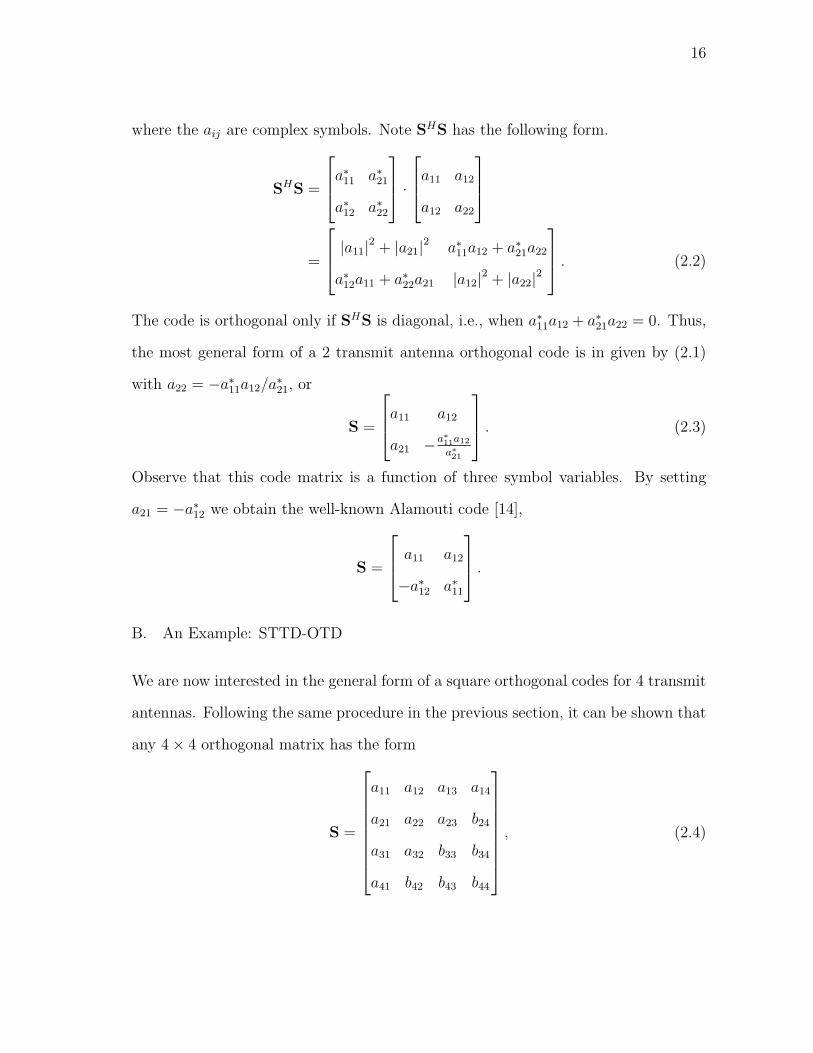
where the aij are complex symbols. Note SHS has the following form.
SHS =
a∗11 a∗21
a∗12 a∗22
·
a11 a12
a12 a22
=
|a11|2 + |a21|2 a∗11a12 + a∗21a22
a∗12a11 + a∗22a21 |a12|2 + |a22|2
. (2.2)
The code is orthogonal only if SHS is diagonal, i.e., when a∗11a12 + a∗21a22 = 0. Thus,
the most general form of a 2 transmit antenna orthogonal code is in given by (2.1)
with a22 = −a∗11a12/a∗21, or
S =
a11 a12
a21 −a∗11a12
a∗21
. (2.3)
Observe that this code matrix is a function of three symbol variables. By setting
a21 = −a∗12 we obtain the well-known Alamouti code [14],
S =
a11 a12
−a∗12 a∗11
.
B. An Example: STTD-OTD
We are now interested in the general form of a square orthogonal codes for 4 transmit
antennas. Following the same procedure in the previous section, it can be shown that
any 4× 4 orthogonal matrix has the form
S =
a11 a12 a13 a14
a21 a22 a23 b24
a31 a32 b33 b34
a41 b42 b43 b44
, (2.4)

17
where
b42 = − (a∗41)−1
[a∗11 a∗21 a∗31
]
a12
a22
a32
,
b33
b43
= −
a31 a32
a41 a42
H
−1
a∗11 + a∗21
a∗12 + a∗22
a13
a23
,
b24
b34
b44
= −
a21 a22 a23
a31 a32 a33
a41 a42 a43
H
−1
a∗11
a∗12
a∗13
a14.
Symbols aij completely specify the space-time code. The elements bij in the lower
right triangle portion of the data matrix are viewed as parity check elements, which
force orthogonality. Define a11 = s1, a12 = s2, a13 = s3, a14 = s4, a21 = −s∗2, a22 = s∗1,
a23 = −s∗4, a31 = s1, a32 = s2, and a41 = −s∗2. Then (2.4) simplifies to
S =
s1 s2 s3 s4
−s∗2 s∗1 −s∗4 s∗3
s1 s2 −s3 −s4
−s∗2 s∗1 s∗4 −s∗3
, (2.5)
which is the STTD-OTD code [25]. Notice we have created an orthogonal code using
this new design approach.

18
C. The New Code Matrix
In (2.4), define a11 = s1, a12 = s2, a13 = s3, a14 = s4, a21 = −s∗2, a22 = s∗1, a23 = −s∗4,
a31 = s3, a32 = s4, and a41 = −s∗4. After simplifying, the code matrix reduces to
S =
s1 s2 s3 s4
−s∗2 s∗1 −s∗4 s∗3
s3 s4 x y
−s∗4 s∗3 −y∗ x∗
, (2.6)
where
x = s1 − ls3,
y = s2 − ls4,
l =< (s1s
∗3 + s2s
∗4)
E= cos (∠s1 − ∠s3) + cos (∠s2 − ∠s4) .
The data matrix (2.6) can be expressed as
S =
s1 s2 s3 s4
−s∗2 s∗1 −s∗4 s∗3
s3 s4 s1 s2
−s∗4 s∗3 −s∗2 s∗1
− l
0 0 0 0
0 0 0 0
0 0 s3 s4
0 0 −s∗4 s∗3
=
A B
B A− lB
, (2.7)
where A and B are Alamouti blocks. Notice the new code resembles the ABBA
code [21] with a new parameter l, which ensures orthogonality.

19
D. Linearity
It is easy to verify that
SHS =
(4∑
i=1
|si|2)
I4. (2.8)
However the optimal receiver for the new code is generally non-linear and cannot
decouple symbols because the code matrix itself is non-linear. This property is char-
acteristic of class I non-linear orthogonal codes. However, the new code will be linear
for symbol constellations where l is constant. In particular, if l = 0,
S =
A B
B A
. (2.9)
This is the ABBA code [21], which is not orthogonal in general, but we show it is
orthogonal for constellations where l = 0.
Notice when symbols s1 and s2 are real and s3 and s4 are imaginary, l = 0.
Thus, for rotated PAM constellations where symbols s3 and s4 are rotated by π/2
with respect to s1 and s2, the new code is linear.
E. Diversity Analysis
If the symbols have the binary constellations,
s1, s2 ∈ ±1,
s3, s4 ∈ ±j,
the code achieves full diversity. In addition, the code is also full rate and linear
(l = 0). Thus, the new code is a complex square orthogonal code with full rate and
diversity for 4 transmit antennas when using this specific rotated BPSK constellation.
Now consider the new code with ordinary QPSK constellations. From perfor-

20
mance plots, it is clear the new code does not have full diversity. One technique to
increase diversity at the expense of data rate is to use a finite state machine (FSM)
to avoid symbol combinations which degrade the diversity of the code.
Before designing a FSM, we first study the code matrix to understand why it
does not achieve full diversity. The new code with QPSK symbols has
• 256 data matrices.
•
256
2
= 256 · 255/2 = 32640 unique data matrix pairs.
• 384 “failing” matrix pairs (which cause the diversity product to be zero).
The failing matrix pairs are pairs of code matrices S and S such that det(S− S
). We
discovered all failing matrix pairs contained at least one code matrix from a small set
of “bad” matrices that must be avoided to achieve full diversity. Before eliminating
all bad matrices with a FSM, constellation phase rotations are used to reduce the
number of bad matrices and optimize data rate. By empirically testing some phase
rotations, it is quickly clear that the number of failing matrix pairs and bad code
matrices can indeed be reduced. Example data is included in Appendix A.
Quite unexpectedly, it was seen that the rotation [φ1, φ2, φ3, φ4] = [0, 1, 3, 5] π/8,
where φi is the counter-clockwise rotation of symbol si, has no failing matrix pairs
(ζv = 0.0058). Thus, full diversity is achieved and a FSM is not needed to improve the
diversity order of the code. With an exhaustive search of all phase shifts in increments
of π/4096, the best phase set found was [0, 0, 32, 19] π/128 (ζv = 0.403775).
There are two key points about this new code. First, with BPSK based con-
stellations it shows that linear complex square orthogonal codes with full rate and
full diversity can exist for specific constellations. Second, we have seen that rotating
symbol constellations is a useful tool to improve diversity.

21
CHAPTER III
A CLASS II NON-LINEAR ORTHOGONAL CODE
In this chapter, we introduce a new class II non-linear orthogonal code.1 The following
heuristic method is used to find the subsequent code. We start with a linear orthog-
onal space-time code with less than full diversity utilizing the appropriate number of
transmit antennas and time intervals per block. To guarantee each symbol is seen
through each channel, the transmitted symbols of the code matrix are encoded with
linear combinations of “base” data symbols. For a fair comparison of performance, the
modification must maintain the same average transmit power. The diversity product
(1.2) is used as a test to search for symbol constellations that allow the modified code
to achieve full diversity. PAM and PSK based constellations are considered.
The new code is developed in Section A. Analysis of code linearity and diversity
are covered in Sections B and C, respectively. In Section D, specific constellations
are designed for the code. It is shown that for PAM based constellations, the code is
a square, full rate, full diversity complex orthogonal design for 4 transmit antennas.
Capacity is discussed in Section E. Finally, in Sections F and G, receivers for when
fading is known and when fading is unknown are outlined, respectively. For known
fading, the optimal receiver decouples the symbol detection problem into pairs. With
PAM based constellations where the code is orthogonal, this receiver simplifies to
complete symbol decoupling.
1See Section D of Chapter 1 for a definition of class II codes.

22
A. The New Code Matrix
Our goal is to design a square, full rate, full diversity, 4 transmit antenna space-time
block code with M -ary constellations. We start with the orthogonal STTD-OTD
code [25] defined as,
S =
s1 s2 s3 s4
−s∗2 s∗1 −s∗4 s∗3
s1 s2 −s3 −s4
−s∗2 s∗1 s∗4 −s∗3
=
A B
A −B
, (3.1)
where A and B are Alamouti blocks. This code alone has a diversity order of 2,
which is easily seen since each symbol is transmitted through only 2 of the 4 transmit
antennas. Since each symbol must be transmitted over every antenna to achieve full
diversity, it is clear that a modification of the code matrix is required. We encode
the transmitted symbols as follows.
s1 =d1 + d2√
2, (3.2)
s2 =d3 + d4√
2, (3.3)
s3 =d1 − d2√
2, (3.4)
s4 =d3 − d4√
2, (3.5)
where d1, d2, d3, and d4 are complex “base” symbols representing the data and s1,
s2, s3, and s4 are complex transmitted symbols. The√
2 is necessary to normalize

23
energy.2 Note the transformation (3.2)–(3.5) can be written as
s1
s2
s3
s4
=1√2
1 1 0 0
0 0 1 1
1 −1 0 0
0 0 1 −1
d1
d2
d3
d4
, (3.6)
or
s1
s3
=
1√2
1 1
1 −1
d1
d2
,
s2
s4
=
1√2
1 1
1 −1
d3
d4
. (3.7)
With this transformation, the new data matrix can be expressed as
S =1√2
d1 + d2 d3 + d4 d1 − d2 d3 − d4
−d∗3 − d∗4 d∗1 + d∗2 −d∗3 + d∗4 d∗1 − d∗2
d1 + d2 d3 + d4 −d1 + d2 −d3 + d4
−d∗3 − d∗4 d∗1 + d∗2 d∗3 − d∗4 −d∗1 + d∗2
=1√2
d1 d3 d1 d3
−d∗3 d∗1 −d∗3 d∗1
d1 d3 −d1 −d3
−d∗3 d∗1 d∗3 −d∗1
+1√2
d2 d4 −d2 −d4
−d∗4 d∗2 d∗4 −d∗2
d2 d4 d2 d4
−d∗4 d∗2 −d∗4 d∗2
=1√2
C C
C −C
+
1√2
D −D
D D
, (3.8)
where C and D are Alamouti blocks.
2We assume the constellations of di, i = 1, . . . , 4, are centered about the origin ofthe complex plane and that each constellation point is equally likely, so E [di] = 0.Then the normalization in (3.2)–(3.5) is valid and the average energies of symbols di
are the same as the average energies of symbols si. For example, E [s1s∗1] = 1
2E [d1d
∗1]+
12E [d2d
∗2] + 1
2E [d1] E [d∗2] + 1
2E [d2] E [d∗1] = E [did
∗i ] = E.

24
B. Linearity
When using a linear transformation like (3.2)–(3.5) on the symbols of a sub-full di-
versity orthogonal space-time code, the receiver will become non-linear for most con-
stellations by introducing quadratic terms into SHS. In this case, SHS for the new
code is non-linear as shown below.
SHS =
|s1|2 + |s2|2 0 0 0
0 |s1|2 + |s2|2 0 0
0 0 |s3|2 + |s4|2 0
0 0 0 |s3|2 + |s4|2
=
(|d1 + d2|2 + |d3 + d4|2)I2 02
02
(|d1 − d2|2 + |d3 − d4|2)I2
=
(∑4i=1 |di|2 + k
)I2 02
02
(∑4i=1 |di|2 − k
)I2
=
(4∑
i=1
|di|2)
I4 + k
I2 02
02 −I2
, (3.9)
where
k = 2< (d1d∗2 + d3d
∗4) . (3.10)
The code is orthogonal in the sense that SHS is diagonal, but the non-linear term
k causes the code to appear quasi-orthogonal in terms of receiver complexity. Thus,
the new code is a class II non-linear orthogonal code.

25
C. Diversity Analysis
Note the following property of determinants:
det
A B
C D
= det (A) det
(D−CA−1B
). (3.11)
To compute the diversity product (1.2) for the new code, (3.11) is used to evaluate
det(S− S
)as shown below.
det(S− S
)= det
A B
A −B
−
A B
A −B
= det(A− A
)det
(−B + B−
(A− A
) (A− A
)−1 (B− B
))
= 4 det(A− A
)det
(B− B
), (3.12)
where S and S are matrices of the form (3.1) and A, A, B, and B are Alamouti
blocks defined accordingly. Furthermore, notice
det(A− A
)= det
s1 s2
−s∗2 s∗1
−
s1 s2
−s2∗ s1
∗
= |s1 − s1|2 + |s2 − s2|2
=1
2
[∣∣∣d1 + d2 − d1 − d2
∣∣∣2
+∣∣∣d3 + d4 − d3 − d4
∣∣∣2]
, (3.13)
where s1 and s2 are symbols in Alamouti block A and definitions for base symbols
d1 through d4 follow from (3.2)–(3.5). For full diversity we require det(A− A
)6= 0
whenever any symbol in S differs from the corresponding symbol in S. Thus,
d1 − d1 + d2 − d2 6= 0, (3.14)
d3 − d3 + d4 − d4 6= 0, (3.15)

26
where (3.14) must hold when d1 6= d1 or d2 6= d2, and (3.15) must hold when d3 6= d3
or d4 6= d4. A similar result follows from det(B− B
).
To design constellations for the new code, first consider (3.14). Note di − di has
a finite number of possible values because di is drawn from a finite size constellation.
As long as the constellation for −d2+ d2 does not contain points that overlap with the
unrotated d1 − d1 constellation (except at the origin where di = di), equation (3.14)
holds. Using similar reasoning, we use (3.15) to design constellations for d3 and d4.
Consider constellations that satisfy (3.14) and (3.15) using symbol phase rotations.
For example, suppose each base symbol has identical constellations, except symbols
d2 and d4 are rotated by an angle φ with respect to d1 and d3. Then the constellations
for d2− d2 and d4− d4 are also rotated by φ with respect to d1− d1 and d3− d3. Since
there are only a discrete number of points in each di− di constellation and an infinite
range of phase rotations, clearly there are infinitely many phase shifts, φ, that offer
full diversity.
D. Constellation Design
1. PAM Based Constellations
Note from (3.9) that any set of symbol constellations such that k = 0 results in a linear
orthogonal code with full diversity, since the coefficients of the energy terms in SHS
are strictly positive. Similarly to the class I non-linear code in the previous chapter,
by restricting base symbols d1 and d3 to be real and d2 and d4 to be imaginary,
k = 0 and SHS =(|d1|2 + |d2|2 + |d3|2 + |d4|2
)I4. Thus, when the base symbols
are drawn from PAM constellations as shown in Fig. 3(a), where symbols d2 and
d4 are rotated by π/2 with respect to real symbols d1 and d3, the code is a square
complex orthogonal design with full diversity. In this case, each transmitted symbol,

27
1d ,
1
d3
432
d , d42
1
2
3
4
(a)
(b)
Fig. 3. (a) Constellations for PAM base symbols; (b) Resulting QAM transmit con-
stellation.
si, i = 1, . . . , 4, is drawn from a QAM constellation as shown in Fig. 3(b). In the
illustration, constellation points are grouped by color. All points of a single color
represent the constellation of d2 (or d4, depending on which si we consider). Each
group is centered on a constellation point in d1 (or d3).
2. PSK Based Constellations
Consider uniform M -PSK base constellations with d2 and d4 rotated by π/M with
respect to d1 and d3. In this case, (3.14) and (3.15) are satisfied and the code will

28
achieve full diversity. QPSK base symbol constellations with d2 and d4 rotated by
π/4 with respect to d1 and d3 are shown in Fig. 4(a). Each transmitted symbol, si,
has 16 possible values depending on the QPSK base symbols, di, as depicted in Fig.
4(b). In the illustration, 4 groups of 4 constellation points are shown with each group
having a different shade of gray. These groups represent the constellation of d2 (or
d4). The center of each group represents the constellation of d1 (or d3). Notice the
phase rotation π/4 maximizes minimum transmitted symbol distance.
One fear in using constellation rotations in practice is a high sensitivity to phase
error. However, this code is relatively robust in the sense that the diversity product
is not vulnerable to a small phase shift error between even (d2 and d4) and odd (d1
and d3) base symbol constellations. This is illustrated in Fig. 5 with a plot of the
diversity product for QPSK symbols. The diversity product is near its maximum
value for a wide range of phases centered about π/4, and is only zero when no phase
shift is used.
E. Capacity
Ignoring the restriction in symbol constellations, we compute the capacity of a MIMO
channel using the new code in (3.8). To compute capacity for one receive antenna,
note equation (1.1) can be converted to the following form,
R = X · H + N, (3.16)

29
1
45
d ,1 d d , d423
4
3
2
43
2 1
(a)
(b)
Fig. 4. (a) Constellations for QPSK base symbols; (b) Resulting transmit constella-
tion.

30
0 0.05 0.1 0.15 0.2 0.25 0.3 0.35 0.4 0.45 0.50
0.1
0.2
0.3
0.4
0.5
φ/π
Div
ersi
ty P
rodu
ct
Fig. 5. Diversity product of the class II non-linear code with QPSK base symbols; d2
and d4 are rotated by φ with respect to d1 and d3.

31
where
R =
[r1 r∗2 r3 r∗4
],
N =
[n1 n∗2 n3 n∗4
],
X =
[d1 d2 d3 d4
],
H =1√2
h1 + h3 h∗2 + h∗4 h1 − h3 h∗2 − h∗4
h1 − h3 h∗2 − h∗4 h1 + h3 h∗2 + h∗4
h2 + h4 −h∗1 − h∗3 h2 − h4 −h∗1 + h∗3
h2 − h4 −h∗1 + h∗3 h2 + h4 −h∗1 − h∗3
, (3.17)
and ri represents the received statistic at time i, ni is the AWGN in ri, hj represents
the channel fading between antenna j and the receive antenna, and di are the base
symbols of the code. In this form, it is clear that the capacity of the new code is
identical to a MIMO channel whose fading matrix is given by H.
Plots of code capacity and optimal capacity for a MIMO channel (1.3) are shown
in Fig. 6 for one receive antenna. The expectations were computed using Monte-Carlo
simulations. Note that capacity of the new code is identical to STTD-OTD and lies
about 2 dB from MIMO capacity.
F. Receivers for Known Fading
1. Optimal Receivers
When fading is known, the optimal receiver decision rule for a space-time block code
is given by
maxS< [
trace(2RHSH−HHSHSH
)]. (3.18)

32
−10 −5 0 5 10 15 20 25 30 350
2
4
6
8
10
12
SNR/information bit (dB)
Cap
acity
(bp
s/H
z)
MIMO STTD−OTD New Ortho
Fig. 6. Capacity of the class II non-linear orthogonal code.

33
With one receive antenna, the decision further simplifies to
maxS
2< (RHSH
)−HHSHSH. (3.19)
For simplicity, assume Nr = 1. In general, the decision rule for the new code with
complex base symbols (e.g., PSK or QAM) follows from (3.19). After simplifying, the
decision rule in terms of si is
maxs1,s3
< (y∗1s1 + y∗3s3)− F1 |s1|2 − F3 |s3|2 , (3.20)
maxs2,s4
< (y∗2s2 + y∗4s4)− F2 |s2|2 − F4 |s4|2 , (3.21)
where the received statistic at time i is denoted ri, the fading over channel j is hj,
and
y1 = x1h∗1 + x∗2h2,
y2 = x1h∗2 − x∗2h1,
y3 = x3h∗3 + x∗4h4,
y4 = x3h∗4 − x∗4h3,
x1 = r1 + r3,
x2 = r2 + r4,
x3 = r1 − r3,
x4 = r2 − r4,
F1 = F2 = |h1|2 + |h2|2 ,
F3 = F4 = |h3|2 + |h4|2 .
We cannot decouple s1 and s3 from s2 and s4 because of their dependence on di. In

34
terms of di, the optimal receiver is,
maxd1,d2
< (r1∗d1 + r2
∗d2 − 2zd1d∗2)− E |d1|2 − E |d2|2 , (3.22)
maxd3,d4
< (r3∗d3 + r4
∗d4 − 2zd3d∗4)− E |d3|2 − E |d4|2 , (3.23)
where
r1 = y1 + y3,
r2 = y1 − y3,
r3 = y2 + y4,
r4 = y2 − y4,
z =1√2
(|h1|2 + |h2|2 − |h3|2 − |h4|2),
E =1√2
Nt∑j=1
|hj|2 .
This verifies that the receiver for the new code is generally not linear because SHS
is non-linear. However, the optimal receiver can at least decouple the base symbols
into pairs. This results in significantly reduced receiver complexity.
a. Using PAM Base Constellations
For an orthogonal code with symbols di and SHS =∑T
i=1 |di|2 INt , the optimal receiver
is linear (with an energy term) and decouples the data symbols. i.e.,
di = arg maxdi
< (diri∗)− Ei |di|2 , i = 1, . . . , 4, (3.24)
where ri is a complex constant and Ei is a real constant.
The detector for our new code using the modified PAM base symbols reduces
to the form (3.24) with ri defined above and Ei = E ∀i. This simplification results

35
because the non-linear terms in (3.22) and (3.23) disappear.
b. Using PSK Base Constellations
For any PSK symbols, the optimal receiver in (3.22) and (3.23) can be simplified.
Since each symbol has equal energy, we have
maxd1,d2
< (r1∗d1 + r2
∗d2 − 2zd1d∗2) , (3.25)
maxd3,d4
< (r3∗d3 + r4
∗d4 − 2zd3d∗4) . (3.26)
2. Sub-Optimal Receivers
A sub-optimal receiver can be derived from (3.20) and (3.21) by decoupling symbols
si, which results in the detection rule (3.24) with ri = yi and Ei = Fi. We compute
a soft estimate of si using
si =yi
2Fi
. (3.27)
From equations (3.2)–(3.5), sub-optimal estimates of base symbols di are generated
by choosing symbols in the constellations of di closest to the following statistics.
d1 =1
2√
2
(y1
F1
+y3
F3
), (3.28)
d2 =1
2√
2
(y1
F1
− y3
F3
), (3.29)
d2 =1
2√
2
(y2
F2
+y4
F4
), (3.30)
d2 =1
2√
2
(y2
F2
− y4
F4
). (3.31)
Sub-optimal zero-forcing (ZF) and linear minimum mean square error (MMSE)
receivers may also be used for simple linear receiver processing. A linear receiver

36
implements,
X = RF, (3.32)
where X and R are defined in Section E. A ZF receiver uses
F = HH(HHH
)−1
, (3.33)
where H is defined in (3.17). A linear MMSE receiver uses
F = HH
(HHH +
1
ρIT
)−1
. (3.34)
The sub-optimal receiver in (3.28)–(3.31) is equivalent to the linear ZF receiver.
G. Receivers for Unknown Known Fading
The optimal receiver for a space-time block code with unknown fading has the decision
rule
minS
trace(RHΓ−1R
)+ ln detΓ,
where
Γ = SSH +1
ρIT ,
and ρ is SNR (we assume symbols in S have unit average energy). If we further
assume a linear orthogonal code with equal energy symbols, then the term detΓ is
not a function of the data. For one receive antenna, the detector reduces to
maxS
RHSSHR.
To estimate the channel, we insert pilot symbols into the data frame and assume
the channel is constant over the entire frame. The transmitted code matrix has the

37
form
S =
P
D
,
where P represents pilot blocks which are known at the receiver, and D represents
data blocks. The received vector has the form
R =
Rp
Rd
,
where Rp is the received pilot block and Rd is the received data block. The optimal
receiver can be expressed as
maxD
2< (RH
d DPHRp
)−RHd DDHRd.
Furthermore, suppose D has the form
D =
D1
D2
...
DBd
,
where Di is the ith transmitted code matrix and Bd is the number data blocks trans-
mitted in a frame. Also, suppose
Rd =
Rd,1
Rd,2
...
Rd,Bd
.

38
Then the optimal receiver has the form
maxD<
(RH
d,1D1H +
Bd∑i=2
Rd,iDi
(H−
i−1∑j=1
DHj Rd,j
)), (3.35)
where H = PHRp. Notice the optimal receiver must jointly detect all code blocks,
Di.
A simpler sub-optimal detector is given by
maxDi
<(RH
d,iDiH)
. (3.36)
This detector uses the pilot block to estimate the channel with H and afterward
assumes this is the exact channel. From (3.35) it is clear this is not an optimal scheme
because it does not take advantage of the data itself to help estimate the channel.
Also notice each code block has been decoupled, and since the code is orthogonal,
each symbol can be decoupled, as in (3.24).

39
CHAPTER IV
PERFORMANCE
Performance of the class I and class II non-linear orthogonal codes are presented in
Section A and B, respectively. For a fair comparison of all simulations, the symbol
energy, E, is normalized by a factor of η/Nt. Thus, the total energy emitted per bit is
the same for all schemes regardless of the number of transmit antennas. Recall that
the channel is modeled with quasi-static fading, in which fading is constant within a
space-time code block and changes independently between blocks.
Most of the following simulation plots compare the new code performance against
ML performance of Papadias’ code [23], the ABBA code [21], the rate 1/2 STTD
orthogonal design [3], the constellation rotating code [27, 28], and STTD-OTD [25]
defined in (3.1). Unless otherwise stated, receivers have perfect knowledge of the
channel. Also, most simulations transmit 2 bits/sec/Hz with QPSK for rate 1 codes,
and 16QAM for the rate 1/2 STTD code [3]. Performance of maximal ratio combining
(MRC) is also presented with SNR normalized by a factor of 6 dB (Nt = 4). This
curve represents a performance goal analogous to MRC compared with the Alamouti
code in the two transmit antenna case.

40
0 2 4 6 8 10 12 14 16 18 2010
−7
10−6
10−5
10−4
10−3
10−2
10−1
100
SNR/information bit (dB)
SE
R (
log
scal
e)
New Code I with QPSK STTD STTD−OTD Papadias/ABBA Rotate MRC + 6dB
Fig. 7. ML performance of the class I non-linear code with QPSK base symbols and
no phase shifts.
A. Class I Non-Linear Code Performance
1. Non-Rotated QPSK Constellations
Consider the new class I non-linear orthogonal code with unrotated QPSK symbols
(spectral efficiency 2). The symbol error rate (SER) for this code and several other
comparable codes are presented in Fig. 7. Observe that the new orthogonal code
outperforms STTD-OTD [25] for SNR above 4 dB and Papadias’ code [23] for SNR
over 12 dB. Below approximately 20 dB, the new orthogonal code also performs better
than the full diversity rate 1/2 STTD code proposed in [3]. Above 14 dB, the complex
constellation rotating code [27], [28] performs better than any other code. From the
slope of the plot, note the new code achieves a diversity order around 3.

41
0 2 4 6 8 10 12 14 16 18 2010
−7
10−6
10−5
10−4
10−3
10−2
10−1
100
SNR/information bit (dB)
SE
R (
log
scal
e)
New Code I with (rotated) QPSK STTD STTD−OTD Papadias/ABBA Rotate MRC + 6 dB
Fig. 8. ML performance of the class I non-linear code with QPSK symbols and phase
shifts [0, 0, 32, 19] π/128.
2. Rotated QPSK Constellations
Using the phase rotation [0, 0, 32, 19] π/128, the new class I non-linear orthogonal
code has full diversity with QPSK symbols. The code SER is presented in Fig. 8 with
other 4 transmit antenna codes using 2 bits/sec/Hz. The performance of the new
code has drastically improved from only a simple constellation phase rotation. It is
now slightly better than the complex constellation rotating code [27], [28] for all SNR
values. However, below 10 dB, Papadias’ code [23] (and equivalent ABBA code [21])
are slightly better than the new code.

42
0 2 4 6 8 10 12 14 16 18 2010
−7
10−6
10−5
10−4
10−3
10−2
10−1
100
SNR/information bit (dB)
SE
R (
log
scal
e)
New Code II with 4−PAM STTD STTD−OTD Papadias/ABBA Rotate MRC + 6 dB
Fig. 9. ML performance of the orthogonal code with 4PAM base symbols and phase
shifts [0, 1, 0, 1] π/2.
B. Class II Non-linear Code Performance
1. Rotated 4-PAM Constellations
Consider the new class II non-linear orthogonal code with rotated 4-PAM symbols,
having an overall spectral efficiency of 2 bits/sec/Hz. The SER for this and several
other comparable codes are presented in Fig. 9. Recall that the new code is an or-
thogonal code and has a linear receiver. The new code performance exceeds that of
all other transmit diversity codes with linear receivers compared. However, Papa-
dias’ code [23] and the ABBA code [21] perform better. The new code with PSK
based constellations motivates the design of similar orthogonal codes with symbol
constellations that have better performance.

43
0 2 4 6 8 10 12 14 16 18 2010
−7
10−6
10−5
10−4
10−3
10−2
10−1
100
SNR/information bit (dB)
SE
R (
log
scal
e)
ZF Linear MMSE STTD MRC + 6 dB
Fig. 10. ZF and linear MMSE performance of the class II non-linear code with QPSK
base symbols and phase shifts [0, 1, 0, 1] π/4.
2. Rotated QPSK Constellations and Linear Receiver
Consider the new class II non-linear orthogonal code with rotated QPSK symbols,
having an overall spectral efficiency of 2 bits/sec/Hz. The SER for this code and the
rate 1/2 STTD orthogonal design [3] with 16QAM are presented in Fig. 10. Note
all codes in the plot have linear receivers. The new code loses diversity when a
sub-optimal ZF or MMSE receiver is used.

44
0 2 4 6 8 10 12 14 16 18 2010
−7
10−6
10−5
10−4
10−3
10−2
10−1
100
SNR/information bit (dB)
SE
R (
log
scal
e)
New Code II with QPSK STTD STTD−OTD Papadias/ABBA Rotate MRC + 6 dB
Fig. 11. ML performance of the class II non-linear code with QPSK base symbols and
phase shifts [0, 1, 0, 1] π/4.
3. Rotated QPSK Constellations and ML Receiver
Consider the new class II non-linear orthogonal code with rotated QPSK symbols,
having an overall spectral efficiency of 2 bits/sec/Hz. The SER for this and several
other comparable codes are presented in Fig. 11. The new code outperforms all other
transmit diversity codes compared. For high SNR, it has a coding gain of more than
1 dB over the next best code, and lies less than 1 dB from the MRC performance
goal.

45
4. Rotated BPSK Constellations and Unknown Fading
In this simulation, the receiver does not know the fading exactly, and uses pilot
symbols to estimate it. These channel estimates are then assumed to be perfect and
used to estimate the data in a frame of several space-time blocks. We assume fading
is constant within a frame (fmT = 0). To compare different pilot symbol schemes,
symbol energy is normalized by the following factor, to transmit a fixed amount of
energy per information bit.
Data Energy/frame
Data Energy/frame + Pilot Energy/frame.
Simulations in Fig. 12 use the sub-optimal receiver in (3.36) with the class II non-
linear orthogonal code and BPSK based symbols. Note this is an orthogonal code.
Performance of the code with known fading is also shown for comparison. Note
performance of the code is severely degraded when the channel is unknown. The best
pilot insertion rate shown is 4/14, which is about 3 dB away from the known fading
curve. Performance does not always improve when using more pilot blocks because
additional pilots must use energy that would have been allocated to data blocks. As
more pilots are added, they do not improve the fading estimate enough to compensate
for the energy normalization.

46
0 2 4 6 8 10 12 14 16 18 2010
−7
10−6
10−5
10−4
10−3
10−2
10−1
100
SNR/information bit (dB)
SE
R (
log
scal
e)
Known fading PIR = 1/11 PIR = 2/12 PIR = 4/14 PIR = 10/20
Fig. 12. Sub-optimal performance in unknown fading (fmT = 0) of the class II
non-linear code with BPSK base symbols and phase shifts [0, 1, 0, 1] π/2.

47
CHAPTER V
CONCLUSION
A. Summary of Results
In Chapter 2, we designed a class I non-linear orthogonal code. The new code with
BPSK constellations proves that linear complex square orthogonal codes with full
rate and full diversity can exist for specific constellations. Also in the analysis of this
code, we have seen that rotating symbol constellations is a useful tool to improve
diversity.
In Chapter 3, a class II non-linear orthogonal code was then presented. We
showed this code has a receiver with moderate complexity, which can decouple sym-
bols into pairs. In general, the new code does not achieve full diversity, but using
constellation phase rotations we showed that full diversity is easily attained. The per-
formance of the new code with rotated PSK based constellations is excellent compared
with other 4 transmit antenna space-time block codes.
From the new class II non-linear orthogonal code of Chapter 3, we created square,
orthogonal, full rate and full diversity space-time code for 4 transmit antennas with
complex M -PAM based constellations. At first, it appears the new code with PAM
base symbols violates the Hurwitz-Radon theorem. However, this theorem has a sub-
tle limitation that is commonly overlooked. It states that square complex orthogonal
designs with full rate and diversity cannot exist, meaning that a general code cannot
exist for all possible symbol constellations. However, one may exist for a specific
restricted constellation. For example, note when complex symbols are confined to
the real line (i.e., for real symbols), orthogonal designs exist for 4 and 8 transmit
antennas. The new orthogonal code with PAM symbols is significant as an existence

48
result, and motivates the search for similar codes with better performance.
A code that is only orthogonal or only has full diversity for specific constellations
is still very practical. The desired data rate of a communication system is typically
known, allowing a system designer to customize a full rate, full diversity code tailored
to meet his specifications.
B. Future Work
The next step in our research is to extend the proposed class II non-linear orthogonal
code to more than 4 transmit antennas. Using these generalized codes as an example,
we will explore and study the existence of linear orthogonal codes using confined
constellation sets. Once these codes are better understood, we can focus on designing
codes with better performance, or possibly developing a useful design criteria.
In this thesis we showed that symbol phase rotations are a useful tool to improve
diversity. This has been noted from many codes, including constellation rotating
codes [27]–[29], for example. These codes are actually class II non-linear orthogonal
codes, and also use constellation phase rotations to attain full diversity. An interesting
direction for research is to study constellation rotations or FSM design techniques
to increase diversity for space-time codes. As a preliminary experiment, we found
Papadias’ code [23], a non-orthogonal code which nearly achieves capacity and has
an elegant sub-optimal linear receiver, can achieve full diversity with rotated QPSK
symbols.
Finally, it is known that full rate delay-optimal orthogonal codes (codes with
minimum T for a given rate and Nt) are not square unless Nt = 2. Designing full
rate non-square orthogonal codes for Nt > 2 remains an interesting problem.

49
REFERENCES
[1] W. C. Jakes, Ed., Microwave Mobile Communications, New York: Wiley, 1974.
[2] G. L. Stuber, Principles of Mobile Communication, Norwell, MA: Kluwer Aca-
demic Publishers, 2nd ed., 2001.
[3] V. Tarokh, H. Jafarkhani and A. R. Calderbank, “Space-time block codes for
orthogonal designs,” IEEE Trans. Inform. Theory, vol. 45, pp. 1456–1466, July
1999.
[4] V. Tarokh, N. Seshadri and A. R. Calderbank, “Space-time codes for high data
rate wireless communication: performance criterion and code construction,”
IEEE Trans. Inform. Theory, vol. 44, pp. 744–765, Mar. 1998.
[5] B. M. Hochwald and W. Sweldens, “Differential unitary space-time modulation,”
IEEE Trans. Commun., vol. 48, pp. 2041–2052, Dec. 2000.
[6] G. J. Foschini and M. J. Gans, “On limits of wireless communication in a fading
environment when using multiple antennas,” Wireless Personal Commun., vol. 6,
pp. 311–335, Mar. 1998.
[7] I. E. Telatar, “Capacity of multi-antenna Gaussian channels,” AT&T Bell Lab-
oratories Internal Tech. Memo., June 1995.
[8] J. G. Foschini, “Layered space-time architecture for wireless communication in
a fading environment when using multi element antennas,” Bell Labs Tech. J.,
vol. 2, pp. 41–59, Autumn 1996.
[9] A. Wittenben, “Base station modulation diversity for digital SIMULCAST,” in
Proc. IEEE Vehicular Tech. Conf. (VTC), St. Louis, MO, May 1991, pp. 848–853.

50
[10] A. Wittenben, “A new bandwidth efficient transmit antenna modulation diver-
sity scheme for linear digital modulation,” in Proc. IEEE Int. Conf. Commun.
(ICC), Geneva, Switzerland, May 1993, pp. 1630–1634.
[11] N. Seshadri and J. H. Winters, “Two signaling schemes for improving the error
performance of FDD transmission systems using transmitter antenna diversity,”
in Proc. IEEE Vehicular Tech. Conf. (VTC), Secaucus, NJ, May 1993, pp. 508–
511.
[12] J. H. Winters, “The diversity gain of transmit diversity in wireless systems with
Rayleigh fading,” in Proc. IEEE Int. Conf. Commun. (ICC), New Orleans, LA,
May 1994, vol. 2, pp. 1121–1125.
[13] A. R. Hammons and H. E. Gamal, “On the theory of space-time codes for PSK
modulation,” IEEE Trans. Inform. Theory, vol. 46, pp. 524–542, Mar. 2000.
[14] S. M. Alamouti, “A simple transmit diversity technique for wireless communica-
tions,” IEEE J. Select Areas Commun., vol. 16, pp. 1451–1458, Oct. 1998.
[15] V. Tarokh, H. Jafarkhani and A. R. Calderbank, “Space-time block coding for
wireless communications: performance results,” IEEE J. Select Areas Commun.,
vol. 17, pp. 451–460, Mar. 1999.
[16] G. Ganesan and P. Stoica, “Space-time diversity using orthogonal and amicable
orthogonal designs,” in Proc. IEEE Int. Conf. Acoust., Speech, Signal Processing
(ICASSP), Istanbul, Turkey, June 2000, pp. 2561–2564.
[17] O. Tirkkonen and A. Hottinen, “Complex space-time block codes for four Tx
antennas,” in GLOBECOM Conf. Records, San Francisco, CA, Nov.–Dec. 2000,
vol. 2, pp. 1005–1009.

51
[18] B. M. Hochwald, T. L. Marzetta and C. B. Papadias, “A novel space-time spread-
ing scheme for wireless CDMA systems,” in Proc. 37th Annual Allerton Conf. on
Commun. Control, and Computing, Monticello, IL, Sept. 1999, pp. 1284–1293.
[19] L. A. Dalton and C. N. Georghiades, “A Four Transmit Antenna Orthogonal
Space-Time Code with Full Diversity and Rate,” in Proc. 40th Annual Allerton
Conf. on Commun. Control, and Computing, Monticello, IL, Oct. 2002.
[20] B. M. Hochwald and T. L. Marzetta, “Unitary space-time modulation for
multiple-antenna communications in Rayleigh flat fading,” IEEE Trans. Inform.
Theory, vol. 46, pp. 543–564, Mar. 2000.
[21] O. Tirkkonen, A. Boariu and A. Hottinen, “Minimal non-orthogonality rate 1
space-time block code for 3+ Tx,” in IEEE Int. Symposium on Spread Spectrum
Techniques & Applications, New Jersey, USA, Sept. 2000, pp. 429–432.
[22] H. Jafarkhani, “A quasi-orthogonal space-time block code,” IEEE Trans. Com-
mun., vol. 49, pp. 1–4, Jan. 2001.
[23] C. B. Papadias and G. J. Foschini, “A space-time coding approach for systems
employing four transmit antennas,” in Proc. IEEE Int. Conf. Acoust., Speech,
Signal Processing (ICASSP), Salt Lake City, Utah, May 2001, pp. 2481–2484.
[24] A. Yongacoglu and M. Siala, “Performance of diversity systems with 2 and 4
transmit antennas,” in Proc. Int. Conf. Commun. Tech. (WCC-ICCT), Peking,
China, 2000, pp. 148–150.
[25] L. M. A. Jalloul, K. Rohani, K. Kuchi and J. Chen, “Performance analysis
of CDMA transmit diversity methods,” in Proc. IEEE Vehicular Tech. Conf.
(VTC), Amsterdam, Netherlands, Oct. 1999, vol. 3, pp. 1326–1330.

52
[26] M. O. Damen, K. Abed-Meraim and J. C. Belfiore, “Transmit diversity using
rotated constellations with Hadamard transform,” in Proc. Adaptive Systems for
Signal Processing, Commun. and Control Conf., Lake Louise, Alberta, Canada,
Oct. 2000, pp. 396-401.
[27] Y. Xin, Z. Wang and G. B. Giannakis, “Linear unitary precoders for maximum
diversity gains with multiple transmit and receive antennas,” in Proc. 34th Asilo-
mar Conf. Signals, Systems, and Computers, Pacific Grove, CA, Oct.–Nov. 2000,
pp. 1553–1557.
[28] Y. Xin, Z. Wang and G. B. Giannakis, “Space-time diversity systems based
on unitary constellation-rotating precoders,” in Proc. IEEE Int. Conf. Acoust.,
Speech, Signal Processing (ICASSP), Salt Lake City, Utah, May 2001, pp. 2429–
2432.
[29] V. M. DaSilva and E. S. Sousa, “Fading-resistant modulation using several trans-
mitter antennas,” IEEE Trans. Commun., vol. 45, pp. 1236–1244, Oct. 1997.
[30] S. Rouquette, S. Merigeault and K. Gosse, “Orthogonal full diversity space-time
block coding based on transmit channel state information for 4 Tx antennas,” in
Proc. IEEE Int. Conf. Commun. (ICC), New York City, NY, April–May 2002,
vol. 1, pp. 558–562.

53
APPENDIX A
FAILING MATRIX PAIRS WITH PHASE SHIFTS
Using the new class I non-linear orthogonal code with QPSK symbols having
counter-clockwise phase shifts [0, 1, 2, 3] π/16, the number of failing matrix pairs was
reduced to 64 from 384. Of these 64 pairs, each contained at least one of the 32 code
matrices from Table I. Thus, by excluding these “bad” matrices, the code can achieve
full diversity.
The symbol constellations are shown in Fig. 13. Table I contains a list of symbol
indices for bad matrices. The symbols in Table I are defined as follows: 1, 2, 3, and 4
represent the constellation points going counter-clock wise around the rotated QPSK
constellation. The “total phase” column contains the sum of the four symbol phases.
Notice the total phase is always 3π/8 or π + 3π/8.

54
Table I. “Bad” matrices for the class I non-linear code with QPSK symbols, phase
shifted by [0, 1, 2, 3] π/16.
s1 s2 s3 s4 Total Phase s1 s2 s3 s4 Total Phase
2 1 1 4 3π/8 4 1 1 2 3π/8
2 1 2 1 π + 3π/8 4 1 2 3 π + 3π/8
2 1 4 3 π + 3π/8 4 1 4 1 π + 3π/8
2 1 3 2 3π/8 4 1 3 4 3π/8
2 2 1 1 π + 3π/8 4 2 1 3 π + 3π/8
2 2 2 2 3π/8 4 2 2 4 3π/8
2 2 4 4 3π/8 4 2 4 2 3π/8
2 2 3 3 π + 3π/8 4 2 3 1 π + 3π/8
2 4 1 3 π + 3π/8 4 4 1 1 π + 3π/8
2 4 2 4 3π/8 4 4 2 2 3π/8
2 4 4 2 3π/8 4 4 4 4 3π/8
2 4 3 1 π + 3π/8 4 4 3 3 π + 3π/8
2 3 1 2 3π/8 4 3 1 4 3π/8
2 3 2 3 π + 3π/8 4 3 2 1 π + 3π/8
2 3 4 1 π + 3π/8 4 3 4 3 π + 3π/8
2 3 3 4 3π/8 4 3 3 2 3π/8

55
��� ���
��� ���
p16
p 8
3p16
�
�
��
�
��
�
Fig. 13. QPSK symbol constellations with phase shifts [0, 1, 2, 3] π/16.

56
VITA
Lori A. Dalton was born in Homestead, FL in 1982. She received her B.S. and
M.S. degrees in electrical engineering from Texas A&M University in 2001 and 2002,
respectively. She is currently a Ph.D. student under Dr. Costas N. Georghiades in
the Wireless Communications Laboratory at Texas A&M University.
Upon admittance to Texas A&M, Ms. Dalton was a recipient of the Texas
A&M Lechner Fellowship in August 1999. She later received TxTEC scholarships
in January 2000 and September 2000, a Nokia scholarship in February 2000, and
a Nortel scholarship in September 2000. She was awarded the Fouraker Graduate
Fellowship and a departmental scholarship in January 2001, and an NSF Graduate
Research Fellowship in March 2001. On November 3, 2001, she was announced Aggie
of the Week during an A&M football game.
In 1998, she worked as a Junior Laureate summer researcher in the DNA De-
partment at the Houston Advanced Research Center in The Woodlands, TX. In the
summer of 2001, she worked in the Wireless Communications Group at Texas Instru-
ments in Dallas, TX. She was also a member of the 2001 Future Energy Challenge
A&M team, which won the nationwide competition. She is a student IEEE member.
In October 2002, she co-authored a paper with Dr. Georghiades entitled, “A Four
Transmit Antenna Orthogonal Space-Time Block Code with Full Diversity and Rate”
in the 40th Annual Allerton Conference on Communication, Control, and Computing.
Her areas of interest include space-time coding, wireless communications, CDMA
and spread spectrum systems, OFDM, digital signal processing, and optical commu-
nications. Her mailing address is 16415 Willow Park Dr., Tomball, TX 77377. Her
email is [email protected].
The typist for this thesis was Ms. Lori Dalton.
Related Documents