UNIVERSITAT DE BARCELONA Departament d’Astronomia i Meteorologia New observational techniques and analysis tools for wide field CCD surveys and high resolution astrometry Mem` oria presentada per Octavi Fors Aldrich per optar al grau de Doctor per la Universitat de Barcelona Barcelona, desembre de 2005

Welcome message from author
This document is posted to help you gain knowledge. Please leave a comment to let me know what you think about it! Share it to your friends and learn new things together.
Transcript

UNIVERSITAT DE BARCELONA
Departament d’Astronomia i Meteorologia
New observational techniques
and analysis tools for wide field
CCD surveys and high
resolution astrometry
Memoria presentada per
Octavi Fors Aldrich
per optar al grau de
Doctor per la Universitat de Barcelona
Barcelona, desembre de 2005


Programa de Doctorat d’Astronomia i Meteorologia
Bienni 1996–1998
Memoria presentada per Octavi Fors Aldrich per optar al grau de
Doctor per la Universitat de Barcelona
Director de la tesi
Dr. Jorge Nunez de Murga


Maite, vull agrair-te tant
temps que fa que t’estimo


Agraıments
Agraıments / Agradecimientos / Acknowledgements
Tota llista d’agraıments es incompleta, i mes quan l’espai de temps es tan dilatat.
Conscient d’aixo, correre el risc de deixar-me algu i, en aquest cas, confio que se’m
disculpi, ja que haura estat per oblit:
Primerament vull donar les gracies al meu director de tesi, en Jorge Nunez de
Murga. Vas donar-me acollida en el teu grup i em consta que has posat a disposicio
meva els elements necessaris (cientıfics, tecnics, etc.) per a que aquesta tesi tires
endavant. Mes enlla del suport cientıfic, el que queda es la relacio personal, la qual
considero ha estat excel.lent. Ha anat madurant lentament, com el bon vi. Per tot
aixo i mes, gracies Jorge.
Vull agrair profundament a l’Albert Prades tot el que he apres d’ell, tant en el
camp cientıfic com en el personal. En el primer, he gaudit llargues i enriquidores con-
verses que, entre d’altres, han servit per incrementar el meu nivell d’autoexigencia
en la feina feta. En el segon, la teva manera d’entendre la vida i la possibilitat
de parlar-ne obertament m’ha permes tirar endavant en moments que em calien
referents i consells de company i amic.
Esctic molt agraıt a en Xavi Otazu, amb qui he tingut la sort de compartir durant
tots aquests anys el seu entusiasme per la ciencia i el seu taranna de treballador
incansable, el qual admiro. A en Xavi li dec la maduracio d’algunes de les idees en
el camp de la deconvolucio astronomica d’imatges que s’exposen en aquesta tesi, aixı
com la utilitzacio del codi de deconvolucio basat en wavelets. Tambe vull expressar
la meva gratitut per tot allo que he apres de tu en el camp informatic, en el que
recordo molt poques ocasions en que no m’hagis satisfet un dubte.

Moltes gracies a la Maite Merino, qui en la darrera etapa de la tesi ha col.laborat
intensament en diversos aspectes de la tesi, com ara les observacions d’ocultacions
lunars a Calar Alto, l’obtencio de les dades de la camera Baker-Nunn de Calgary i
la sistematica i enriquidora revisio d’aquesta tesi. A mes a mes, li agraeixo espe-
cialment el seu esperit altruısta en tasques de logıstica de grup sense les quals la
finalizacio d’aquesta tesi hauria estat mes perllongada.
Vull fer un agraıment especial al Dr. Codina, director de l’Observatori Fabra.
Ha estat tot un honor col.laborar amb l’Observatori i poder compartir aquests anys
de treball amb el qui ha estat un excel.lent cap, docent, pero sobretot un senyor
com en queden pocs. Amb el temps, els seus consells en moments importants han
resultat sempre encertats. Finalment, vull agrair-li que hagi fet seu el projecte
de robotitzacio de la camera Baker-Nunn de San Fernando, que juntament amb en
Jorge Nunez, vam imaginar per primera vegada un dia de novembre de 2000. Aquest
gran esforc ha estat essencial per a superar tots els alts i baixos d’un projecte que,
tot just ara, albira un horitzo de futur immediat.
Tambe vull donar les gracies a tot el personal de l’Observatori Fabra durant
aquest anys: en Nicolau Torras, l’Antonio Gazquez, en Jaume Perez, en Dionıs
Escamez, en Marc Prohom, l’Alfons Puertas, la Teresa Susagna, la Marta Gonzalez
i en Ramon Secanell. Gracies a ells m’he sentit com a casa i han fet possible que
la tasca realitzada a l’Observatori fos encara mes realitzant. Finalment, un record
especial per als companys de l’Observatori que ja no romanen entre nosaltres: en
Joan Pardo, l’Enric Santamaria i la Maria Campo. De tots ells, pero en especial
d’en Joan, vaig sentir innumerables relats sobre l’Observatori d’un valor, almenys
simbolic, incalculable i que algu hauria d’afanyar-se a recollir per escrit ja que formen
part de la memoria col.lectiva de la ciutat de Barcelona i del paıs.
Al meu company de despatx i amic Marc Ribo mai li prodre estar prou agraıt.
Possiblement, ell sigui qui millor conegui els detalls cotidians del camı que he hagut
de fer per arribar fins aquı. Sempre que m’ha calgut ajuda de qualsevol tipus
(cientıfica, informatica, personal), un consell, en definitiva, un amic, en Marc era
allı. La seva gran valua com a cientıfic rivalitza amb la qualitat humana que transmet
als altres.
Gracies a la colla d’amics de la Facultat. Molt especialment, gracies al David
Nofre i el seu germa Jordi i al Nestor i l’Astrid. Amb tots quatre he passat es-
tones inolvidables que m’han donat aire per seguir amb la tesi. Cinemes, sopars,

excursions, viatges d’estiu, tot plegat quelcom que he grabat per sempre en la retina
vital.
Tambe vull tenir un agraıment per en Valentı Bosch, qui ha ocupat el lloc d’en
Marc en aquests darrers anys. Has estat un excel.lent company de despatx, amb el
qui he pogut compartir coneixement i idees de tot tipus: cientıfiques, informatiques,
fins i tot polıtiques. Gracies tambe a en Pol Bordas, que s’ha afegit a la colla de la
galera 756 en aquest darrer any i amb qui he mantingut tambe converses interessants
i m’ha assistit amb el meu italia elemental.
Moltes gracies als doctorands (be, la majoria ja sou il.lustres doctors) del De-
partament d’Astronomia i Meteorologia per deixar-me compartir dinars, sopars de
festa, sortides d’observacio, excursions, etc. M’ho he passat molt be i mirant enrere
considero que som uns privilegiats quan hem pogut fer recerca en un ambient de
companyonia com el del poble. Moltes gracies Marc, Xavi, David, Montse, Mai-
te Beltran, Ricard, Marta, Lola, Ignasi, Albert Domingo, Eduard, Merce, Oscar,
Imma, Teresa, Josep Miquel, Pep, Andreu Raig, Angels, Ada i un llarg etcetera.
A en Jose Ramon Rodrıguez (per tots conegut com a JR) li resto profundament
agraıt principalment per dues coses. En primer lloc per la seva extraordinaria profes-
sionalitat i eficiencia en la Secretaria del Departament d’Astronomia i Meteorologia.
Davant de la meva manifesta incompetencia a l’hora de gestionar paperassa, has
estat el meu angel de la guarda sense el qual no se que hauria passat. En segon lloc,
gracies per ajudar-me a comprendre la complexitat que comporta un departament
universitari com el DAM. Certament, ha estat un exercici de Psicologia de grups
interessant.
I would like to express my gratitude to Bill van Altena for the constant support
and assistance received while my three research stays at Yale. What I learned about
astrometry at those meetings in your group has turned out to be of crucial value
for the development of this thesis. The same gratitude applies for all members of
your group: Terry Girard, Imants and Vera Platais, Dana Dinescu, Reed Meyer and
John Lee. I enjoyed a fruitful scientific experience among all of you. In the personal
side, I discovered you all are wonderful people and I often miss you. Voldria tambe
agrair a la Carme Gallart tota la hospitalitat que em va demostrar durant el temps
que vam coincidir a Yale.
I would like to acknowledge here my gratitude to Andrea Richichi. His great

scientific enthusiasm encouraged me to pursue the Calar Alto Lunar Occultation
Program and their different data analysis derivatives, both projects being essential
parts of this thesis. I am also in debt to you for all the assistance and guidance you
offered me in the field of lunar occultations. On the personal side, I have always
felt like having a close and sincere relationship with you. I also thank you and ESO
Director General Discretionary Funding Program (DGDF) for making possible the
numerous visits both of us have made to Barcelona and Garching.
Tambien mi mas sincera gratitud a todos los observadores que han participado
en los numerosos perıodos de observacion del programa de ocultaciones lunares de
Calar Alto, y al que tanto debe esta tesis. Muchas gracias a Maite Merino, Javier
Montojo, Jorge Nunez, Xavier Otazu, Dolores Perez, Albert Prades y Andrea Ric-
hichi. Vuestro esfuerzo vale su peso en oro, mas teniendo en cuenta que en ningun
momento os vencio el desanimo incluso en las repetidas noches en blanco que cosec-
hamos debido al mal tiempo en Calar Alto. Coordinar este equipo humano ha sido
todo un placer para mı.
A deep thanks to Elliott Horch, whose expertise in the field of speckle interfe-
rometry helped me to develop a substantial part of this thesis. I greatly enjoyed
sharing exciting discussions about instrumental aspects of CCD speckle and bispec-
tral analysis while your visit to Barcelona. Thanks for making understandable what
is not obvious for others. I guess you learnt this gift from Bill van Altena.
I am deeply grateful for the assistance of Kenneth Mighell, who shared his great
expertise about PSF fitting and centering algorithms during the last months of this
thesis. Although by email, the outstanding level of his dissertations allowed my to
madurated some of the fundamental concepts exposed in this thesis.
I am indebted to Christoph Flohr, for attending my request of adapting his
drift-scanning program SCAN for lunar occultations and speckle interferometry ob-
servations. His expertise in the knowledge of CCD adquisition software has been
enlightening for the proper course of this thesis.
Thanks also to Craig Markwardt, who kindly provided the IDL subroutines which
I adapted for centering stars by means of the Levenberg-Marquardt technique for
non-linear least squares curve fitting.
Although we never have met in person, thanks to Michael Richmond from Roc-

hester Institute of Technology, who kindly attended all my questions about image
processing and coordinates matching algorithms.
A big thanks to Roy Tucker, who assisted me in all sort of questions about
drift-scanning technique and their instrumental side aspects.
This research has made use of the SIMBAD database, operated at CDS, Stras-
bourg, France. This thesis makes use of data products from the Two Micron All
Sky Survey, which is a joint project of the University of Massachusetts and the
Infrared Processing and Analysis Center/California Institute of Technology, funded
by the National Aeronautics and Space Administration and the National Science
Foundation.
Tambien estoy en deuda con el personal astronomico de soporte del Centro As-
tronomico Hispano-Aleman (CAHA) y de la Estacion de Observacion de Calar Alto
(EOCA) del Observatorio Astronomico Nacional (OAN). Muy especialmente qui-
ero agradecer la eficiente ayuda prestada por Santos Pedraz, Ulli Thiele y Javier
Alcolea, sin los cuales las observaciones incluidas en esta tesis hubieran sido poco
mas que imposibles. Finalmente, un reconocimiento a todo el personal astronomico
y administracion del CAHA y OAN que durante todos estos anos de estancias de
observacion me hayan hecho sentir como en casa, sobretodo en los parones por mal
tiempo.
Agraeixo a la Reial Academia de Ciencies de Barcelona (RACAB) per la beca
pre-doctoral de Formacio de Personal Investigador que vaig gaudir en el perıode
01/1997-12/1997.
Agradezco a la Direccion General de Ensenanza Superior e Investigacion Ci-
entıfica, Ministerio de Educacion y Cultura (MEC) por la beca pre-doctoral de
Formacion de Personal Investigador (FPI), ref. AP97 38107939, que disfrute en el
perıodo 01/1998-06/2001.
Un profund agraıment per la Judit, la meva germana, qui m’ha ajudat a superar
entrebancs que s’han anat presentant durant aquesta tesi. I no nomes em refereixo
als nombrosos favors que t’he demanat (gestions a la Caixa de Catalunya per viatges,
estades d’observacio, etc.), sino al fet de ser allı sempre disposada a escoltar. Ha estat
molt improtant per mı disposar d’un referent addicional als pares mentre vivıem
plegats.

Un gracies ben fort i sentit als meus pares Josep Maria i Marta. Ara caig que
es la primera vegada que tinc l’oportunitat d’agrair-vos per escrit tot el que heu
fet per mi com a pares. Durant tot aquest camı m’heu donat suport sentimental,
sostingut economicament i educat en uns valors i actituds que m’han permes, entre
d’altres coses, realitzar aquesta tesi. M’heu sapigut escoltar tant en els alts com
en els baixos que he anat atravessant, i els vostres consells m’han ajudat a que els
segons fossin cada cop mes superables. Moltes gracies pares.
I per acabar, gracies a la Maite, la dona de la meva vida. Molts/es dels que
llegeixin aixo coincidiran amb mi en que la recerca, com altres activitats professionals
que involucren gran dedicacio, a voltes es difıcilment conjugable amb la vida normal
de parella. No nomes ho has acceptat, sino que m’has encoratjat a seguir endavant
en tot moment, conscient que aixo implicava renunciar a un trocet de la nostra
vida. Des de les trucades kilometriques des dels USA fins els caps de setmana
d’aquest darrer any esmercats en la recta final de la tesi, sempre t’he tingut al meu
costat. Per brillar com el millor dels estels quan tornava a casa, per fer-me sentir
algu important en els moments durs, per ajudar-me a organitzar l’escas temps que
sobretot en la darrera etapa disposava, per suportar-me quan tornava amb mal
humor, per escoltar-me i cuidar-me, per estimar-me, per tot aixo i per molt mes,
GRACIES.

Contents
Resum de la tesi: Noves tecniques observacionals i eines d’analisi per
a observacions CCD de gran camp i astrometria d’alta resolucio ix
1 Introduction and background 1
1.1 Deconvolution in astronomy . . . . . . . . . . . . . . . . . . . . . . . 1
1.1.1 Applications of deconvolution . . . . . . . . . . . . . . . . . . 3
1.1.2 Motivations and scope of Part I . . . . . . . . . . . . . . . . . 7
1.2 New observational techniques and analysis tools in high resolution
astrometry . . . . . . . . . . . . . . . . . . . . . . . . . . . . . . . . . 9
1.2.1 Lunar occultations . . . . . . . . . . . . . . . . . . . . . . . . 10
1.2.2 Speckle interferometry . . . . . . . . . . . . . . . . . . . . . . 18
1.2.3 Motivations of Part II . . . . . . . . . . . . . . . . . . . . . . 19
I Application of image deconvolution to wide field CCDsurveys 31
2 Image deconvolution 33
2.1 Basis . . . . . . . . . . . . . . . . . . . . . . . . . . . . . . . . . . . . 33
i

ii CONTENTS
2.1.1 Image formation and representation . . . . . . . . . . . . . . . 34
2.1.2 Point-spread function and sampling . . . . . . . . . . . . . . . 35
2.1.3 Noise . . . . . . . . . . . . . . . . . . . . . . . . . . . . . . . . 39
2.1.4 Image deconvolution: an ill-conditioned inverse problem . . . . 40
2.2 Maximum Likelihood Estimator . . . . . . . . . . . . . . . . . . . . . 41
2.3 AWMLE: Adaptive Wavelet-based Maximum Likelihood Estimator . 43
2.3.1 Wavelets overview . . . . . . . . . . . . . . . . . . . . . . . . . 43
2.3.2 Adaptive algorithm . . . . . . . . . . . . . . . . . . . . . . . . 45
2.3.3 AWMLE computational performance . . . . . . . . . . . . . . 48
2.4 Deconvolution and sampling . . . . . . . . . . . . . . . . . . . . . . . 49
3 Data description 51
3.1 Data acquisition schemes . . . . . . . . . . . . . . . . . . . . . . . . . 52
3.1.1 Stare observing mode . . . . . . . . . . . . . . . . . . . . . . . 54
3.1.2 Drift scanning observing mode . . . . . . . . . . . . . . . . . . 58
3.1.3 TDI observing mode . . . . . . . . . . . . . . . . . . . . . . . 69
3.1.4 Discussion . . . . . . . . . . . . . . . . . . . . . . . . . . . . . 74
3.2 Data sets description . . . . . . . . . . . . . . . . . . . . . . . . . . . 75
3.2.1 Flagstaff Astrometric Transit Telescope (FASTT) . . . . . . . 76
3.2.2 QUasar Equatorial Survey Team (QUEST) . . . . . . . . . . . 87
3.2.3 NESS-T: Baker-Nunn camera at Rothney Astrophysical Ob-
servatory . . . . . . . . . . . . . . . . . . . . . . . . . . . . . . 96

CONTENTS iii
4 Proposed methodology 105
4.1 Generic CCD reduction . . . . . . . . . . . . . . . . . . . . . . . . . . 105
4.2 PSF fitting . . . . . . . . . . . . . . . . . . . . . . . . . . . . . . . . 107
4.3 Object detection . . . . . . . . . . . . . . . . . . . . . . . . . . . . . 112
4.4 Increase in SNR and limiting magnitude . . . . . . . . . . . . . . . . 114
4.4.1 Validation with a deeper and higher resolution image . . . . . 115
4.4.2 Validation with reference catalogue . . . . . . . . . . . . . . . 115
4.4.3 Validation with multiframe comparison . . . . . . . . . . . . . 116
4.5 Increase in limiting resolution . . . . . . . . . . . . . . . . . . . . . . 118
4.5.1 Qualitative assessment of resolution gain . . . . . . . . . . . . 119
4.5.2 Quantitative assessment of resolution gain . . . . . . . . . . . 120
4.6 Source centering . . . . . . . . . . . . . . . . . . . . . . . . . . . . . . 120
4.6.1 Deconvolution and centering . . . . . . . . . . . . . . . . . . . 122
4.6.2 Levenberg-Marquardt Method . . . . . . . . . . . . . . . . . . 122
4.7 Astrometric assessment . . . . . . . . . . . . . . . . . . . . . . . . . . 124
5 Results 127
5.1 PSF fitting . . . . . . . . . . . . . . . . . . . . . . . . . . . . . . . . 127
5.1.1 FASTT . . . . . . . . . . . . . . . . . . . . . . . . . . . . . . 127
5.1.2 QUEST . . . . . . . . . . . . . . . . . . . . . . . . . . . . . . 129
5.1.3 NESS-T . . . . . . . . . . . . . . . . . . . . . . . . . . . . . . 131
5.2 Deconvolution convergence . . . . . . . . . . . . . . . . . . . . . . . . 132

iv CONTENTS
5.3 Increase in SNR and limiting magnitude . . . . . . . . . . . . . . . . 133
5.3.1 QUEST . . . . . . . . . . . . . . . . . . . . . . . . . . . . . . 133
5.3.2 NESS-T . . . . . . . . . . . . . . . . . . . . . . . . . . . . . . 151
5.4 Increase in resolution and object deblending . . . . . . . . . . . . . . 167
5.4.1 QUEST: QSO candidates deblending for gravitational lenses
detection . . . . . . . . . . . . . . . . . . . . . . . . . . . . . . 167
5.4.2 NESS-T . . . . . . . . . . . . . . . . . . . . . . . . . . . . . . 191
5.5 Astrometric assessment . . . . . . . . . . . . . . . . . . . . . . . . . . 200
5.5.1 FASTT . . . . . . . . . . . . . . . . . . . . . . . . . . . . . . 201
6 Conclusions 205
II New observational techniques and analysis tools forhigh resolution astrometry 221
7 Lunar occultations 223
7.1 Phenomenon description . . . . . . . . . . . . . . . . . . . . . . . . . 223
7.1.1 Observational constraints . . . . . . . . . . . . . . . . . . . . . 225
7.1.2 LO lightcurve model . . . . . . . . . . . . . . . . . . . . . . . 227
7.2 Data acquisition techniques . . . . . . . . . . . . . . . . . . . . . . . 228
7.2.1 CCD fast drift scanning . . . . . . . . . . . . . . . . . . . . . 229
7.2.2 IR arrays subarray . . . . . . . . . . . . . . . . . . . . . . . . 234
7.3 Events prediction: inclusion of 2MASS Point Source Catalogue . . . . 235
7.4 Data description . . . . . . . . . . . . . . . . . . . . . . . . . . . . . 238

CONTENTS v
7.4.1 Fabra Observatory . . . . . . . . . . . . . . . . . . . . . . . . 238
7.4.2 CALOP: Calar Alto Lunar Occultation Program . . . . . . . . 241
7.5 Data reduction and analysis . . . . . . . . . . . . . . . . . . . . . . . 246
7.5.1 ALOR . . . . . . . . . . . . . . . . . . . . . . . . . . . . . . . . 246
7.5.2 CAL . . . . . . . . . . . . . . . . . . . . . . . . . . . . . . . . . 247
7.5.3 Automatic reduction with wavelet analysis . . . . . . . . . . . 248
7.6 Fabra results . . . . . . . . . . . . . . . . . . . . . . . . . . . . . . . 261
7.6.1 SAO 77911 . . . . . . . . . . . . . . . . . . . . . . . . . . . . 261
7.6.2 SAO 79031 . . . . . . . . . . . . . . . . . . . . . . . . . . . . 262
7.7 CALOP results . . . . . . . . . . . . . . . . . . . . . . . . . . . . . . 264
7.7.1 Binaries . . . . . . . . . . . . . . . . . . . . . . . . . . . . . . 265
7.7.2 Diameters . . . . . . . . . . . . . . . . . . . . . . . . . . . . . 274
7.7.3 Limiting magnitude . . . . . . . . . . . . . . . . . . . . . . . . 278
7.7.4 Limiting resolution . . . . . . . . . . . . . . . . . . . . . . . . 281
7.7.5 Binary detection probability . . . . . . . . . . . . . . . . . . . 283
7.7.6 Upcoming improvements in detectors technologies . . . . . . . 284
7.8 Conclusions . . . . . . . . . . . . . . . . . . . . . . . . . . . . . . . . 286
7.9 Work in progress and future plans . . . . . . . . . . . . . . . . . . . . 288
7.9.1 Speckle follow-up observations . . . . . . . . . . . . . . . . . . 288
7.9.2 CALOP-II: extension to a long-term remotely operated program289
7.9.3 Special events . . . . . . . . . . . . . . . . . . . . . . . . . . . 293
7.9.4 Galactic center passages at VLT . . . . . . . . . . . . . . . . . 295

vi CONTENTS
7.9.5 Close binaries detection with wavelet analysis . . . . . . . . . 296
8 Speckle interferometry 305
8.1 Overview . . . . . . . . . . . . . . . . . . . . . . . . . . . . . . . . . . 305
8.2 Data acquisition techniques . . . . . . . . . . . . . . . . . . . . . . . 307
8.2.1 Speckle in large format CCDs . . . . . . . . . . . . . . . . . . 307
8.2.2 Fast drift scanning technique . . . . . . . . . . . . . . . . . . 309
8.3 Data description . . . . . . . . . . . . . . . . . . . . . . . . . . . . . 311
8.4 Data reduction and analysis . . . . . . . . . . . . . . . . . . . . . . . 313
8.4.1 Self-calibration scheme . . . . . . . . . . . . . . . . . . . . . . 313
8.5 Results . . . . . . . . . . . . . . . . . . . . . . . . . . . . . . . . . . . 318
8.6 Limitations of self-calibration technique . . . . . . . . . . . . . . . . . 323
8.7 Upcoming CCD improvements . . . . . . . . . . . . . . . . . . . . . . 323
8.8 Conclusions . . . . . . . . . . . . . . . . . . . . . . . . . . . . . . . . 325
III General conclusions 337
A Project of automatization of a Baker-Nunn camera 345
A.1 Brief historical overview . . . . . . . . . . . . . . . . . . . . . . . . . 346
A.2 Original instrument description . . . . . . . . . . . . . . . . . . . . . 347
A.3 Refurbishment project . . . . . . . . . . . . . . . . . . . . . . . . . . 348
A.3.1 Optical refiguring . . . . . . . . . . . . . . . . . . . . . . . . . 350
A.3.2 Mechanical modification . . . . . . . . . . . . . . . . . . . . . 355

CONTENTS vii
A.3.3 CCD support . . . . . . . . . . . . . . . . . . . . . . . . . . . 358
A.3.4 Observing site and operational modes . . . . . . . . . . . . . . 359
A.3.5 Observatory control system . . . . . . . . . . . . . . . . . . . 361
A.4 Data acquisition schemes . . . . . . . . . . . . . . . . . . . . . . . . . 363
A.4.1 Stare mode . . . . . . . . . . . . . . . . . . . . . . . . . . . . 364
A.4.2 TDI mode . . . . . . . . . . . . . . . . . . . . . . . . . . . . . 365
A.5 Scientific project . . . . . . . . . . . . . . . . . . . . . . . . . . . . . 367
A.5.1 QDSS: Quick Daily Sky Survey . . . . . . . . . . . . . . . . . 367
A.5.2 Specific observational programs . . . . . . . . . . . . . . . . . 369
B SNR performance of PEPs and CCDs in LO 375
C List of observed LO events in CALOP 381

viii CONTENTS

Resum de la tesi: Noves tecniques
observacionals i eines d’analisi per
a observacions CCD de gran camp
i astrometria d’alta resolucio
1. Introduccio
Aquesta tesi es divideix en dues parts diferenciades. La primera part versa sobre
l’aplicacio de la deconvolucio a imatges CCD de gran camp i els beneficis que se
n’obtenen. La segona es centra en el desenvolupament de noves tecniques observaci-
onals i d’analisi de dades en els camps de les ocultacions lunars i la interferometria
speckle.
1.1 Deconvolucio d’imatges
La deconvolucio d’imatges preten substraure d’una imatge tots aquells efectes dis-
torsionadors que en el seu proces de formacio ha incorporat. Els principals son la
funcio de distorsio puntual (PSF) i el soroll. La primera esta causada per la tur-
bulencia atmosferica, l’optica del telescopi i el proces de mostreig. El segon, en els
cas dels detectors CCDs, es composa del soroll de conteig Poisson i el sorroll de
lectura del mateix detector.
La tasca d’eliminar aquests efectes condueix a una equacio inversa mal condi-
cionada, la solucio de la qual no te assegurada l’estabilitat ni la unicitat. S’han
ix

x Resum de la tesi
proposat una gran varietat d’algoritmes en la literatura per assegurar l’anterior.
Les diferencies entre ells poden raure en quatre punts: la hipotesis de formacio de la
imatge, les restriccions de regularitzacio emprades per assegurar la unicitat i estabi-
litat de la solucio, les tecniques numeriques considerades per cercar la convegencia i
els tests de validacio per avaluar el grau de convergencia. En aquesta tesi utilitzarem
dos d’aquests algorismes: el Richardson-Lucy (Lucy 1974) o la seva variant per a
soroll Poissonia i Gaussia (MLE) (Nunez & Llacer 1993), i el Metode Adaptatiu de
Maxima Versemblanca basat en Wavelets (AWMLE) (Otazu 2001). Aquest darrer
destaca per mostrar una convergencia assimptotica i un bon control d’amplificacio
de soroll amb el nombre d’iteracions.
Les aplicacions dels algorismes de deconvolucio en el camp de l’Astronomia ha
estat molt variades. Aquestes es distribueixen al llarg d’un ampli rang de longitud
d’ona, relacio-senyal-soroll (SNR), resolucio, context astrofısic, etc. Per enumerar-ne
nomes unes quantes, anant de longituts d’ona mes llargues a mes curtes:
� primer survey optic-VLA (Haarsma et al. 2005),
� deconvolucio del perfil radial HI en superfıcie de galaxies espirals (Noordermeer
et al. 2005),� millora de la resolucio espacial d’observacions submil.limetriques SCUBA d’ob-
jectes estel.lars joves (Krause et al. 2003),
� millora de resolucio en imatges d’optica adaptativa ESO 3.6 m/ADONIS del
volcanisme de Io en el infraroig mitja (Marchis et al. 2000),
� millora de resolucio de cloves de pols a l’entorn d’estrelles de carboni (Bontekoe
et al. 1994),� increment de la deteccio de quasars lensats en el infraroig amb VLT/ISAAC (Fau-
re et al. 2003),� Analisi de lens gravitacionals febles a l’entorn de galaxies properes amb dades
HST/ACS (Jee et al. 2005),� estudi de l’estructura de jet i disc de l’objecte jove triple HV Tauri (Stapelfeldt
et al. 2003),� eliminacio de les distorsion d’astigmatisme i coma de l’arxiu de plaques fo-
tografiques de l’Observatori de Sonneberg (Hiltner et al. 2003)

Resum de la tesi xi
� millora de la deteccio d’estructures nebulars i jets optics en objectes BL Lac
objects a OJ 287 Benitez et al. (1996),
� guany en la deteccio d’un outburst de la estrella Mira A en rajos X Chan-
dra (Karovska et al. 2005),
� deteccio de hypernoves en spectres γ amb dades INTEGRAL (Schanne & et
al. 2004).
Com s’observa, els proposits de l’aplicacio de la deconvolucio rauen tıpicament
en la millora de la resolucio, la detectabilitat d’objectes febles, la supressio de dis-
torsions de la imatge original.
Una caracterıstica comu a totes aquestes aplicacions es que s’han dut a terme
amb telescopis grans, camps de visio reduıts i detectors de la mes alta qualitat, on
sovint la relacio SNR de les dades es alta i la PSF i el soroll es poden caracteritzar
molt acuradament. A mes a mes, quasi totes elles son observacions puntuals relatives
a l’estudi d’un objecte i no son sistematiques, es a dir, no cobreixen grans arees de
cel durant un temps continuat (tipus survey). Hi ha diverses raons que justifiquen
aquesta aplicacio selectiva. En primer lloc, l’esforc necessari per a la deconvolucio
sistematica d’un joc de dades survey es mes complexe i requereix la utilitzacio d’eines
d’analisi especialitzades. Segon, el rendiment cientıfic en aplicacions selectives de
gran qualitat esta assegurat en la majoria dels casos mentre que en el cas survey no
sempre. Finalment, el cost computacional de la deconvolucio es elevat i requereix
un esforc addicional quan el volum de dades a reduır es gran.
1.2 Ocultacions lunars
Una ocultacio lunar s’esdeve quan la Lluna s’interposa en la lınia visual entre una
estrella i l’observador. Degut que la naturalesa ondulatoria de la llum, la intensitat
de la estrella no minva instantaniament, sino que ho fa en uns ∼ 0.1s. La distribucio
d’intensitat de l’estrella durant aquest interval de temps es pot aproximar a la predita
per la difraccio de Fresnel d’una font puntual monocromatica ocultada per una
pantalla rectilınia. La modelitzacio del fenomen pot ser completada amb la inclusio
de la policromia de la font, fonts resoltes o multiples i d’altres efectes instrumentals
com ara el soroll de centelleig i la influencia del diametre del telescopi, el filtre o el
mostreig temporal.

xii Resum de la tesi
D’entre totes les aplicacions que se’ls ha donat a les ocultacions lunars (LO), les
dues seguents son les que actualment son vigents en l’Astronomia moderna:
� determinacio de diametres estelars de fins 1 mil.lisegon d’arc (mas) amb una
incertesa tıpica del ∼ 5%. Aquestes mesures, que es duen a terme en el visible
i IR, son possibles si la SNR de les dades es prou alta (>10). Els diametres
obtinguts son de gran utilitat per a validar models d’evolucio estelar a partir
d’incerteses en les temperatures efectives < 50 K. Tambe s’utilitzen per l’estudi
estructural de fonts no esfericament simetriques com ara estrelles pulsants
i estudi d’envolcalls circumstelars (Mondal & Chandrasekhar 2005; Ragland
et al. 1997; Richichi et al. 1988), fonts Mira (Mondal & Chandrasekhar 2004),
etc. La calibracio de teperatures efectives per a les estrelles mes fredes del
diagrama H-R, tipus espectral K, M i de carboni, tambe s’han beneficiat de
les mesures de diametres proporcionades per les LO (Richichi et al. 1999).
� deteccio de binaries de separacio projectada fins a 1 mas i relacions de brillantor
de 1:1 a 1:150. Les aplicacions en aquest camp d’estudi son, apart de la deteccio
en sı, la determinacio de l’orbita i les masses del sistema binari. En aquest
darrer camp, Evans (1983); Richichi et al. (2000) han desenvolupat una intensa
activitat observadora amb milers d’ocultacions enregistrades i una probabilitat
de deteccio d’una binaria del ∼ 10%. Una darrera lınia d’aplicacio ha estat
l’estudi de la frequencia de binaritat d’objectes joves T Tauri. A partir de
mesures LO (Chen & Simon 1997; Leinert et al. 1991; Simon et al. 1995, 1996,
1999) han mostrat que aquest escenari de formacio estelar esta dominat per
la presencia de sistemes multiples.
Les LO presenten avantatges i inconvenients respecte altres tecniques d’alta re-
solucio espacial:
Per una banda, els interferometres optics de llarga base que entraran a ple rendi-
ment en breu (VLTI, Keck) requereixen per a la seva calibracio d’un cataleg de fonts
resoltes per les quals es conegui previament el seu diameter. Les LO son actualment
la unica tecnica que pot subministrar aquestes mesures amb suficient nombre i pre-
cisio. Un altre avantatge de les LO es que no son fenomens limitats per la difraccio
del telescopi. Finalment, es una tecnica instrumentalment barata ja que precisa
telescopis de 1− 2 metres amb instrumentacio convencional (fotometres o cameres
IR).

Resum de la tesi xiii
Per altra banda, les LO son esdeveniments fixats en el temps i que estan res-
tringits a la franja zodiacal del cel (un 10% del total) on la Lluna projecta la seva
orbita. Tambe cal afegir que els parametres mesurats per a una estrela binaria no
son els reals, sino els projectats al llarg de la direccio d’escombrat de la Lluna.
1.3 Interferometria speckle
La interferometria speckle es una tecnica observacional que permet extraure infor-
macio espacial de l’objecte observat per sota el lımit de difraccio del telescopi. Aixo
s’aconsegueix per mitja de l’enregistrament rapid (mostreig ∼ 10 ms) i successiu
d’exposicions del objecte en questio. Aixı, la turbulencia atmosferica fracciona el
front d’ona en diverses regions (o speckles). En aquestes condicions de mostreig,
aquestes es poden considerar coherents i estacionaries per cadascun dels fotogrames
mostrejats.
Les resolucions que tıpicament s’aconsegueixen oscilen entre 0.′′01 i 1.′′0. Aquest
rang se situa enmig del que altres tecniques d’alta resolucio venen subministrant
(observacions visuals amb micrometre i els mes moderns interferometres optics, res-
pectivament).
El camp principal d’estudi de les mesures speckle han estat les estrelles binaries
i el calcul de les seves orbites, que constitueixen un primer pas per a l’establiment
de la Relacio Massa–Lluminositat i la Funcio Initial de Massa. Aquesta tasca s’ha
realitzat gracies a la observacio sistematica d’aquestes per part de nombrosos grups
durant mes de 25 anys (Balega et al. 2004; Docobo et al. 2004; Hartkopf et al. 2000;
Horch et al. 2004; Mason et al. 2004; Saha et al. 2002; Scardia et al. 2005).
Els requeriments instrumentals de la interferometria speckle son: mostreig rapid,
baix soroll de lectura, alta eficiencia quantica i linearitat. La majoria de les observa-
cions anteriorment citades han estat dutes a terme amb detectors CCD intensificats
(ICCD), que combinen caracterıstiques del fotometres i les cameres CCD. Els ICCDs
satisfan la majoria dels anteriors requeriments tecnics. Han mostrat deficiencies en
la linelitat, cosa que ha conduit a una perdua en la precisio fotometrica.
Paralelament, els CCDs no intesificats han anat incrementant la seva rapidesa,
eficiencia quantica i linealitat i reduint el seu soroll de lectura. Com a resultat, noves
tecniques d’adquisicio amb CCD han estat proposades amb exit Horch et al. (1997,

xiv Resum de la tesi
2001); Zadnik (1993).
1.4 Motivacio de la tesi
Pel que fa a la deconvolucio:
Per una banda, com hem vist els surveys mai han estat motiu d’aplicacio de les
tecniques de deconvolucio. Per altra banda, la computacio distribuida esta assolint
rendiments de calcul cada cop mes grans. Tambe val a dir que el problema de la
deconvolucio d’imatges es facilment escalable. A mes a mes, cal tenir en compte
que no totes i cadascuna de les imatges captades per un d’aquests projectes hauria
de ser subceptible de ser deconvolucionada. Estrategies de seleccio de camps mes
petits basats en informacio previa poder ajudar i molt al rendiment del metode
de deconvolucio en programes de cerca d’objectes especıfics com ara macrolensing,
GRBs, NEOs, etc.
Tot plegat ens duu a pensar que la deconvolucio d’un banc de dades provinent
d’un projecte tipus survey podria ser factible i objecte d’estudi en aquesta part de
la tesi, la qual preten assolir els seguents objectius:
1. definir i implementar una metodologia general que permeti deconvolucionar
imatges CCD generiques de tipus survey.
2. mostrar que la aplicacio de la deconvolucio amb l’algorisme AWMLE millora
l’eficiencia observacional, concretament la magnitud limit i la resolucio limit de
les imatges. Per exemple, una millora en la magnitud lımit de ∆mlim ∼0.6 mag
equivaldria a incrementar el diametre del telescopi (D) en un 30%. Tenint en
compte que el cost d’un telescopi es proporcional a D2.7 (Andersen & Christen-
sen 2000; Meinel & Meinel 1980; Schmidt-Kaler & Rucks 1997; Sebring et al.
2000), queda clar que la deconvolucio pot ser altament efectiva des del punt
de vista economic.
3. clarificar quina incidencia sobre la presicio astrometrica introdueix la decon-
volucio.
El punt 2 es especialment pertinent per aquells surveys que degut a les seves
particularitats en el metode d’adquisicio o sistema optic, han vist rebaixades les

Resum de la tesi xv
seves magnitud i resolucion lımit.
Pel que fa a les ocultacions lunars:
El panorama descrit en l’apartat anterior es susceptible de canviar en un futur
proper degut a les seguents consideracions:
En primer lloc, els catalegs actuals en IR han incrementat en diversos ordres
de magnitud el seu nombre d’objectes. Per exemple, mentre que el cataleg Two
Micron Sky Survey (TMSS) (Neugebauer & Leighton 1969) nomes era complet fins
a magnitud K . 3, el nou 2MASS (Cutri et al. 2003) ha extes la seva mostra fins
a Klim ∼ 14.3, amb prop de 500 milions d’objectes. Consequentment, el nombre
d’ocultacions potencials en una nit amb un telescopi de 1.5 m ha passat de 20-30 a
mes de 100.
En segon lloc, els detectors CCD i cameres infrarojes han millorat les seves
prestacions en termes d’eficiencia quantica, soroll de lectura i frequencia de mostreig.
Tot i oferir mes avantatges que el fotometres unidimensionals, aquest dos tipus de
detectors no han estat emprats regularment per observar LO.
Ateses aquestes consideracions, hem cregut oportu fixar els seguents objectius:
1. desenvolupar, implementar i validar una nova tecnica d’observacio de LO per
CCDs. Apart de la consideracio anterior respecte la millor constant en aquests
detectors, cal tenir en compte que els CCDs son presents a la majoria dels
observatoris. El seu interes es, per tant, justificat.
2. disenyar i implementar un nou algorisme de reduccio automatic de LO, que
permeti reduir grans nombres d’ocultacions en poc temps i de manera no
supervisada. Aquest punt es fa essencial ates el gran increment d’ocultacions
potencials que els nous catalegs han aportat.
3. impulsar i portar a terme un programa d’observacio de LO intensiu centrat en
la deteccio de noves binaries.
Pel que fa a la interferometria speckle:
Ateses les consideracions descrites en l’anterior apartat, hem establert els seguents
objectius en aquest apartat de la tesi:

xvi Resum de la tesi
1. desenvolupar una nova tecnica observacional basada en CCD no intensificat
que permeti realitzar observacions speckle de precisio.
2. validar l’anterior tecnica amb l’observacio d’estrelles binaries que tinguin una
orbita ben coneguda.
3. proposar i desenvolupar un nou metode de calibracio per a les dades speckle
que permeti observacions mes eficients.
2. Aplicacio de la deconvolucio d’imatges a obser-
vacions CCD de gran camp
2.1 Algorismes emprats, dades i procediment
Com hem esmentat en la instroduccio, hem treballat amb dos tipus d’algorismes de
deconvolucio: el MLE i el AWMLE.
El MLE presentat per Nunez & Llacer (1993) pren en consideracio una modelit-
zacio correcta del soroll en la imatge CCD. A partir d’aquı construeix una funcio de
versemblanca que maximitza per mitja de la tecnica de les substitucions successives.
Es tracta, per tant, d’un algorisme iteratiu no lineal. Aixo comporta problemes de
convergencia cap a la solucio fısicament desitjada, ja que si deixem iterar el MLe
suficientment aquest amplifica el soroll present en la imatge original. Com a solucio
parcial, s’acostuma a aturar la convergencia a un nombre d’iteracions prudent.
El AWMLE representa l’evolucio del MLE (fa servir el mateix estimador es-
tadıstic) per a solucionar d’una manera natural l’amplificacio del soroll. Aixo s’a-
consegueix amb la descomposicio de la imatge original en una base de funcions
anomenades wavelets. Aquestes permeten obtenir una bona localitzacio espacial
dels diferents detalls frequencials de la imatge (tambe anomenats planols wave-
let). D’aquesta manera, la deconvolucio pot operar de manera selectiva en segons
quins planols i regions estadısticament significatives (no relatives a soroll). Es trac-
ta, doncs, d’un algorisme adaptatiu que no amplifica el soroll i presenta una con-
vergencia assimptotica (elimina la necessitat d’aturar arbitrariament).
Una caracterıstica comuna d’ambdos algorismes es l’evolucio del mostreig en

Resum de la tesi xvii
la imatge deconvolucionada. S’ha mostrat que aquest tendeix a empitjorar amb
el nombre d’iteracions (Prades & Nunez 1997; Prades et al. 1997). Aquest efecte
ve acompanyat de l’aparicio d’un artifacte anomenat ringing i que consisteix en
oscil.lacions d’intesitat al voltant de les estrelles mes brillants. El ringing pot ser
eliminat en ambdos algorismes si l’usuari es capac de modelar amb precisio l’emissio
de fons (background) de la imatge original.
Per tal de mostrar els beneficis de la deconvolucio d’imatges a observacions CCD
de gran camp, hem disposat de tres jocs de dades, provinent de tres surveys: el
Flagstaff Transit Telescope (FASTT), el QUasar Equatorial Survey Team (QUEST)
i el Near-Earth Space Surveillance Terrestrial (NESS-T).
FASTT es un telescopi meridia de l’Observatori Naval d’Estats Units que realitza
observacions astrometriques de gran precisio, per tal de densificar catalegs com
ara HIPPARCOS i Tycho. Es tracta, doncs, d’un instrument extraordinariament
calibrat i precıs des del punt de vista astrometric. Es per aquesta rao que hem escollit
el FASTT per a avaluar l’impacte de la deconvolucio sobre la precisio astrometrica.
QUEST es un telescopi tipus Schmidt situat a Venezuela amb una camera CCD
mosaic de gran format, i coordinat per la Universitat de Yale, el Centro de Investiga-
ciones de Astronomıa (CIDA), la Universidad de Los Andes (ULA) i la Universitat
d’Indiana. Centra el seu estudi a elaborar un cens de quasars complet fins magnitud
mB ∼ 21. A resultes d’aquest cataleg, s’espera obtenir una fraccio significativa de
lents gravitatories que permeti verificar questions fonamentals de la teoria de Rela-
tivitat General. L’estrategia d’observacio consisteix en obtenir una mostra de can-
didats a quasars per mitja del criteri de variabilitat fotometrica. Aquests candidats
son posteriorment confirmats o desmentits amb observacions de suport (follow-up),
espectroscopiques i d’imatge, en un telescopi de diametre major (WIYN). Gracies
al gran camp i la magnitud profunda de QUEST, el conjunt de candidats pot ser
molt nombros (> 104). Es fa necessari, per tant, un metode complementari que
permeti refinar la llista de candidats, retenint aquells que podrien ser susceptibles
de ser lensats. Aquesta es la tasca que hem dut a terme aplicant la deconvolucio
AWMLE a dos camps QUEST-WIYN.
NESS-T es un projecte dedicat al cens de NEOs operat pel Rothney Astrophy-
sical Observatory i la Universitat de Calgary. L’instrument emprat es una camera
Baker-Nunn de gran camp (4.◦4x4.◦4). La relacio focal extraordinariament curta d’a-
quest instrument fa que el mostreig de la imatge estigui dominat per la figura de

xviii Resum de la tesi
merit del sistema optic (no pel seeing). Com a resultat, les dades NESS-T presen-
ten un elevat deblending entre estrelles properes, que fa pertinent l’aplicacio de la
deconvolucio AWMLE.
Mentre que FASTT i QUEST han seguit el mode d’observacio anomenat drift-
scanning, NESS-T ho ha fet per mitja de l’standard o stare. El mode drift-scanning
consisteix en aturar el seguiment del telescopi, alinear l’eix de transferencia de
carrega del CCD amb l’equador celest i acomodar el ritme d’ aquesta amb el si-
deri, que es amb el que la imatge de les estrelles es trasllada sobre el detector.
Aquest mode presenta diversos avantatges i inconvenients. Per una banda, es mes
eficient en termes d’area observada per unitat de temps, ja que eliminat el temps
mort dedicat al reapuntat del telescopi i la lectura de la camera CCD. Per altra ban-
da, la magnitut lımit de les observacions esta limitada al ritme sideri d’escombrat.
Tambe introdueix una serie de distorsions en la PSF de les estrelles que impliquen
una perdua significativa de SNR i resolucio. Hem aplicat la deconvolucio AWMLE
per tal de compersar aquests darreres restriccions inherents al drift-scanning.
Una de les aportacions d’aquesta part de la tesi es la definicio d’una metodologia
general que permet aplicar l’aplicacio de la deconvolucio d’imatges (MLE, AWMLE
o qualsevol altre algorisme) a un joc de dades de caracterıstiques generiques (tipus
stare o drift scanning). El procediment proposat es divideix en dues fases: la previa
i la posterior a la deconvolucio.
La fase previa a la deconvolucio preten aconseguir una caracteritzacio precisa
de les dades originals. En altres paraules, volem obtenir una estimacio realista de
la PSF, el background, el guany i el soroll de lectura de la imatge original. Totes
aquests valors s’han obtingut per mitja d’un conjunt d’eines d’analisi ben establertes
que s’utilitzen pel mateix proposit en altres camps de l’Astronomia.
La fase posterior a la deconvolucio es centra en l’analisi dels resultats per mitja
de tres descriptors: el guany en magnitud lımit, el guany en resolucio i l’impacte
sobre l’error astrometric. Pels tres subprocediments cal efectuar una validacio dels
objectes detectats tant en la imatge original com deconvolucionada. Aquest es
realitza amb una imatge d’alta resolucio de referencia o un cataleg astrometric mes
complet.

Resum de la tesi xix
2.2 Resultats
Magnitud lımit
Aquest estudi s’ha realitzat aplicant els algorismes AWMLE i MLE a les dades
QUEST i NESS-T. Es tracta de calcular quin es la magnitud lımit abans i despres
de deconvolucionar, tot emprant la metodologia proposada en l’apartat anterior.
S’han trobat valors de ∆Rlim ∼ 0.64 i ∆Rlim ∼ 0.46 per les dades QUEST i
NESS-T, respectivament. Il.lustrem el guany obtingut per les dades QUEST en la
Fig. 1, on es mostra l’histograma de magnitud pels objectes detectats en la imatge
original i deconvolucionada amb AWMLE despres de 750 iteracions. Val a dir que
aquest guany equival a un increment d’un 81% en el nombre d’objectes nous recupe-
rats que poden ser mesurats i que no estaven disponibles en la imatge original. En
termes d’increment d’area col.lectora el guany es tradueix en un augment del 32%
en diametre del telescopi, que suposa multiplicar el cost del mateix per 2.3.
6 8 10 12 14 16 18 20WIYN instrumental magnitude
0
10
20
30
40
# de
tect
ions
AWMLE 750 iterationsOriginal
��������������������
Figura 1: Histograma de magnitud de deteccions per la imatge QUEST original i la
deconvolucionada amb 750 iteracions AWMLE.
Com a resultat paral.lel de l’anterior guany, s’ha pogut investigar l’existencia
d’algun objecte amb interes astrofısic entre les deteccions noves aportades per la
deconvolucio AWMLE. Efectivament, tal com mostra la Fig. 2 s’ha trobat un possible
esdeveniment de magnitud transitoria (transient) de magnitud en les dades QUEST.
Hem discutit la possible associacio d’aquest fenomen amb una estrella binaria de

xx Resum de la tesi
rajos X de l’Halo Galactic.
0891−0539099
E6
C6
C6 C6
E6E6
E6
C6
Figura 2: E6, la mes brillant de les noves deteccions sense parella trobades en la imatge
de referencia (WIYN), gracies a la deconvolucio AWMLE. Superior esquerra: Imatge
original QUEST. Superior dreta: Deconvolucio AWMLE QUEST 750 iteracions. Inferior
esquerra: Imatge WIYN del mateix camp. Inferior dreta: Deconvolucio AWMLE WIYN
150 iteracions. L’objecte central en vermell correspon a l’estrella V = 14.7 USNO-
B1.0 0891-0539099. El cercle verd correspon a la nova deteccio desaparellada en la
imatge QUEST deconvolucionada: els quadrats verds en la resta de panells indiquen la
no-deteccio en la posicio hipotetica de E6 en cada imatge. En blau, una estrella de
comaparacio C6 amb una separacio angular respecte USNO-B1.0 0891-0539099 molt
semblant a la d’E6. Noteu que en la imatge QUEST original tant E6 com C6 es poden
intuir marginalment sota les ales de l’objecte brillant central. Les magnituds estimades
per E6 i C6 son V ∼ 19.9 i V ∼ 20.4, respectivament. Val a dir que, malgrat la
molt mes feble magnitud lımit en la imatge WIYN (Vlim ∼ 23.6), E6 no es detecta allı.
Apuntem la possible associacio d’aquest fenomen transitori de mes de 3 magnituds com
una estrella binaria de rajos X de l’Halo Galactic.

Resum de la tesi xxi
La convergencia assimptotica del metode AWMLE ha propiciat una eficiencia
excepcional en la deteccio de nous objectes. Concretament, s’ha vist que el metode
de deconvolucio no introdueix practicament cap deteccio falsa i que s’arriba a aquesta
solucio independentment del nombre d’iteracions i el dintell de deteccio emprat.
Aquest resultat confirma allo apuntat en la presentacio del metode i que la teoria
de funcions wavelet indicava.
Resolucio lımit
Aquest estudi preten quantificar la resolucio (∆φlim) que l’algorisme AWMLE
ha estat capac d’injectar (o recuperar) en relacio a la imatge original. Altre cop
la metodologia introduıda en l’apartat anterior detalla com hem procedit en aquest
estudi.
S’han calculat identics valors de ∆φlim ∼ 1 pixel per les dades QUEST i NESS-
T, o equivalentment a ∆φQUESTlim ∼ 1.′′0 i ∆φNESS−T
lim ∼ 3.′′9, respectivament. Aquests
valors es deriven de la separacio angular mınima entre dos objectes resolts en amb-
dues imatge, l’original i la deconvolucionada. La Fig. 3 ens mostra la distribucio
12 13 14 15 16 17 18m2 of resolved component
0
2
4
6
8
ρ (a
rcse
c)
Figura 3: Separacio angular de les components resoltes al camps QUEST graficada
en funcio de la magnitud WIYN. El punts verds indiquen que l’objecte es present a
les tres imatges, els vermells els que son a la imatge WYIN de referencia i la QUEST
deconvolucionada, pero no a la QUEST original i els blaus els que nomes son a la WIYN.
d’aquestes separacions mınimes en funcio de la magnitud de l’objecte mes feble (o

xxii Resum de la tesi
secundari). Com s’observa, la deconvolucio AWMLE (punts vermells) permet resol-
dre objectes mes propers i amb una magnitud mes feble que no pas la imatge original
(punts verds). S’ha comprobat que aquest guany depen fortament del mostreig de
la imatge original i molt lleument de altres factors com ara els errors sistematics
deguts al mode d’adquisicio drift scanning or el coneixement limitat en el modelatge
de la PSF.
Candidate 2
Candidate 5
Candidate 3
C2 C2
C5C5
C2
C5
C3C3C3
B
B
D
EF
C
BC
Figura 4: Tres candidats a quasars amb diferents estats de resolucio. Per a cada panell,
esquerra: imatge QUEST original, centre: QUEST deconvolucionada, dreta: WIYN de
referencia. C2 representa un exemple de candidat no resolt en cap de les tres imatges.
C3 es un cas d’objecte crıticament no resolt en la imatge QUEST deconvolucionada. C5
ha estat resolt en la QUEST deconvolucionada pero no en la QUEST original.
Com en el cas de l’estudi de magnitud lımit, hem considerat un cas particular
d’objectes en les imatges QUEST i NESS-T que poguessin beneficiar-se de l’anterior

Resum de la tesi xxiii
guany en resolucio. En el cas del QUEST, ho hem aplicat a uns col.lecio de 44
candidats a quasars detectats pel criteri de variabilitat fotometrica. La deconvolucio
ens ha permes resoldre per primer cop alguns d’aquests candidats, tot confirmant-
los amb la imatge d’alta resolucio i amb mes magnitud lımit WIYN. La Fig. 4
ilustra tres casos tıpics de candidats deconvolucionats: C2 no resolt, C3 crıticament
resolt (l’elongacio augmenta) i C5 resolt. Aquest darrer podria ser susceptible de
ser observat amb un telescopi major i amb espectroscopia, per tal de confirmar o no
si es tracta d’un quasar lensat.
Precisio astrometrica
Diversos autors han mostrat resultats apuntant que la deconvolucio d’imatges
podria empitjorar l’error astrometric o introduir un biaix posicional cap al centre del
pixel (Girard 1995). Hem utilizat les dades FASTT per reproduir aquest experiments
amb l’aplicacio de l’algorisme MLE (el mateix emprat en l’anterior estudi).
Les dispersions dels residus a la imatge original i deconvolucionada han estat:
� σorigx , σorig
y =(0.057,0.041) pixels per les imatges originals,
� σdeconvx , σdeconv
y =(0.059,0.046) pixels per les imatges deconvolucionades.
El lleuger increment per la segona no es pot considerar significatiu, sobretot
perque el biaix assimetric que existia en el nuvol original ha estat efectivament
eliminat per la deconvolucio. A mes a mes, no s’ha observat biax posicional cap al
centre del pixel.
Com a punt decisiu d’aquest resultat destaquem que hem utilitzat una nova
eina de centrat d’objectes basada en el metode de Levenberg-Marquardt. Aquesta
ha demostrat ser menys sensible al submostreig que les tecniques convencionals.
Com a exemple d’aquesta robustesa, aquest ha pogut ajustar correctament perfils
estelars de FWHM fins a 0.8 pixels mentre que la resta d’algorisme divergien a
FWHM∼ 1.5 pixels.

xxiv Resum de la tesi
3. Noves tecniques observacionals i d’analisi de da-
des per l’astrometria d’alta resolucio
3.1 Nou metode d’observacio fast drift scanning
Tant pel que fa a les observacions de LO com d’interferometria speckle, hem coin-
cidit a assenyalar que un rapid mostreig temporal es essencial per a una correcta
representacio del fenomen. En ambdos casos aquest ha de ser de l’ordre d’uns pocs
mil.lisegons.
Per tal de complaure aquestes necessitats, s’ha ideat, implementat i avaluat una
nova tecnica d’observacio CCD anomenada fast drift scanning. En termes generals,
aquesta consisteix en reduir la quantitat de pixels que han de ser transferits en
cada mostra i accelerar el ritme de lectura tant com el modul digitalizador de la
camera CCD permeti. Com a resultat, el ritme de mostreig augmenta, que es el que
preteniem.
Aquest nou metode d’adquisicio no implica cap modificacio optica ni mecanica
adicional en el telescopi. Per tant, es molt indicada per a observatoris professionals
de baix pressupost i aficionats de perfil alt que vulguin iniciar programes d’observacio
en LO i interferometria speckle.
3.2 Observacions d’ocultacions lunars
En el cas particular de les LO, el fast drift scanning ens ha permes mostrejar cada
2 ms, que es l’optim per un telescopi del rang 1–2 m.
En paral.lel al desenvolupament d’aquesta nova tecnica, es va endegar un nou
programa d’ocultacions a llarg termini (4 anys). Aquest va ser dut a terme a l’Ob-
servatori de Calar Alto (Almerıa) en els telescopis OAN 1.5 m i CAHA 2.2 m, tant
en la banda visible com en la infraroja (IR), i rep el nom de CALOP. En el primer
cas, es va utilitzar la tecnica fast drift scanning amb una camera CCD comercial.
En el segon cas, s’empra la camera IR MAGIC (Herbst et al. 1993) en el mode de
lectura subarray, que era conegut amb anterioritat. Aquest esforc observacional es
perllonga durant 71.5 nits produint 388 ocultacions enregistrades.

Resum de la tesi xxv
Els resultats inclouen la deteccio d’un sistema triple (IRC-30319) i 14 binaries
noves i 1 de coneguda en l’IR proper, i una binaria nova en el visible. Les seves sepa-
racions projectades estan compreses entre 0.′′09 i 0.′′002, amb relacions de brillantor
fins a 1:35 en la banda K. Tambe s’ha mesurat els seguents diametres angulars:
� 30 Psc (φUD = 6.78± 0.07 mas) en el visible,
� V349 Gem (φUD = 5.10± 0.08 mas) en l’IR,
� RZ Ari (φUD = 10.6± 0.2 mas) en l’IR. La Fig. 5 il.lustra l’ajust realitzat per
obtenir l’anterior diametre amb l’algorisme ALOR (Richichi 1989).
La Taula 1 inclou un sumari mes compet dels resultats obtinguts en el programa
CALOP.
Taula 1: Sumari dels resultats obtinguts de les observacions del programa CALOP.
(1) (2) (3) (4) (5) (6) (7) (8) (9) (10)
Source |V| (m/ms) V/Vt–1 ψ(◦) PA(◦) CA(◦) SNR Sep. (mas) Br. Ratio φUD (mas)
SAO 164567 0.6443 3% − (74) (11) 14.3 2.0 ± 0.1 1.7 ± 0.1
30 Psc 0.2473 −44% 20 122 69 46.1 6.78± 0.07
SAO 78119 0.5387 −3% 2 129 41 52.7 13.1 ± 1.1 34.2 ± 2.5
V349 Gem 0.9462 −2% 8 106 11 65.9 5.10± 0.08
SAO 78258 0.6307 2% 1 45 −50 9.4 47.3 ± 1.5 8.6 ± 0.7
AG+24 788 0.6910 3% 6 75 −13 16.9 28.8 ± 0.7 4.9 ± 0.2
SAO 79251 0.7215 −1% −1 85 −15 20.2 26.9 ± 1.1 17.6 ± 1.5
SAO 80764 0.6568 −3% −2 73 −45 26.3 42.5± 0.3 14.9± 0.3
SAO 185661 0.3287 −5% −2 155 60 23.7 37.9± 1.1 19.3± 0.7
IRC -30319 A-B 0.5647 3% 2 136 44 52.6 15.0± 0.1 8.74± 0.04
IRC -30319 B-C 16.1 21.8± 0.1 2.98± 0.01
17454891-2809333 0.7720 4% 3 98 6 25.0 39.3± 0.7 17.3± 0.9
SAO 165154 0.5870 24% 14 117 62 6.2 43.0± 1.9 4.7± 0.4
RZ Ari 0.6520 −2% 10 73 11 41.3 10.6± 0.2
SAO 76214 A-C 0.3500 −5% −2 131 56 7.8 13.0± 0.7 2.4± 0.1
IRAS 04395+2521 0.6301 11% 8 135 49 21.4 6.5± 0.2 2.9± 0.1
04440885+2540333 0.8013 −0% −0 77 −10 3.9 15.6± 0.8 1.4± 0.1
05415664+2707323 0.9208 −2% −3 108 12 17.4 24.8± 0.3 7.8± 0.3
HD 283610 0.5244 −5% −3 121 38 9.1 19.4± 0.7 6.1± 0.3
04264187+2500314 (0.8900) − − (86) (0) 3.8 89.5± 1.0 2.5± 0.1
SAO 77000 0.4995 2% −2 109 37 16.0 12.6± 0.3 1.49± 0.03
Tambe es va mesurar l’eficiencia de CALOP en termes de magnitud lımit i re-
solucio lımit. Ambdos parametres son claus per a coneixer les limitacions que el
programa te amb la instrumentacio actualment utilitzada. Com a resultat s’ha ob-
tingut unes magnituds lımit Klim ∼ 8.0 i ≈ 9.0, pels telescopis OAN 1.5 m i CAHA

xxvi Resum de la tesi
2.2 m. Pel que fa a les resolucions lımit, es van estimar φlim entre 1-3 mas, respecti-
vament.
0
20000
40000
60000
80000In
tens
ity (c
ount
s)
1900 2000 2100 2200 2300Relative intensity (ms)
-10000
-5000
0
5000
10000
Figura 5: Superior: Corba de llum de RZ Ari (negre) i ajust amb algorisme ALOR
(vermell) corresponent a un diametre de φUD = 10.6± 0.2 mas. Inferior: Residus.
La probabilitat de deteccio de binaries ha estat calculada a l’entorn del ≈ 4%.
Aquest valor es significavament menor que l’obtingut en altres programes d’observa-
cio similars (Richichi et al. 1996). Atribuım aquest defecte de binaries al fet que hem
utilitzat un cataleg (2MASS) amb una densitat d’estrelles molt major als anteriors
estudis per a elaborar les predicions.
Com una altra contribucio desenvolupada en aquest apartat de la tesi, i davant
del gran nombre d’ocultacions mesurades, ens vam veure en la necessitat de desen-
volupar una nova eina de reduccio automatica basada en la transformada wavelet
de la corba de llum de l’ocultacio. En aquest cas unidimensional, aquesta base de
funcions ens permet localitzar molt eficientment el canvi d’intensitat degut a l’ocul-
tacio, destriant-lo de manera molt robusta de les oscil.lacions degudes al soroll de la
camera o al centelleig atmosferic. Una bona mostra de la robustesa d’aquesta nova
eina queda il.lustrada en la Fig. 6.
Finalment, dins del programa CALOP s’inclou una nova serie d’ocultacions per
pasos de la Lluna per Centre Galactic. Aquesta s’inicia amb l’observacio el dia 28

Resum de la tesi xxvii
0 20000 40000 60000100
300
500
700
1500 2000 2500 3000 3500100
300
500
700
0 20000 40000 60000150
250
350
450
1500 2000 2500 3000 3500150
250
350
450
0 20000 40000 60000100200300400500600700800
1500 2000 2500 3000 3500100200300400500600700800
0 20000 40000 600000
500
1000
1500
2000
2000 2500 3000 3500 40000
500
1000
1500
2000
0 20000 40000 60000100
150
200
250
300
350
1000 1500 2000 2500 3000100
150
200
250
300
350
t0 �������
t0 ���� ���
t0 ������
t0 ���� ����
t0 �������
Figura 6: Aplicacio d’un criteri basat en wavelets per trobar l’instant d’ocultacio t0 per
a 5 corbes de llum amb diferents valors de SNR (de dalt a baix: 20, 10, 5, 2 i 1).
Panells de l’esquerra representen la totalitat de les corbes de llum (d diversos segons
de durada). Els panells drets representen la porcio de la corba de llum a l’entorn del
t0 trobat automaticament. Noteu que fins i tot en el cas de SNR=1, t0 es localitzat
correctament.

xxviii Resum de la tesi
de Juliol de 2004. Vam obtenir 54 ocultacions en 3.4h (1.5h de temps efectiu), gran
part de les quals son fonts infrarojes sense contrapartida optica, i de les quals s’ha
derivat multiplicitat per primer cop (veure IRC -30319 en la Taula 1). Aquest tipus
d’esdeveniments donen l’oportunitat d’extraure informacio del millisegon d’arc en
regions poc estudiades.
3.3 Observacions d’interferometria speckle
En el cas particular de la interferometia speckle, s’ha adaptar la tecnica d’observacio
CCD drift scanning per assolir els ritmes de mostreigs requerits (poques desenes de
mil.lisegonds per fotograma speckle).
De manera similar al que es va fer amb les ocultacions lunars, es va dur a terme un
perıode d’observacio a l’Observatori de Calar Alto per a validar aquesta nova tecnica.
El telescopi escollir va ser l’OAN 1.5 m amb la mateixa camera CCD emprada per les
campanyes d’ocultacions. Es van observar 4 binaries d’orbita coneguda. En la Fig. 7
il.lustrem una sequencia de fotogrames speckle obtinguts en aquelles condicions pel
sistema doble ADS 755.
0 50 100 150 200 250 300Pixels
Figura 7: Tira de fotogrames speckle enregistrats per mitja de la tecnica drift scanning
per la estrella binaria ADS755. Els fotogrames son de 20x20 pixels i el temps d’exposicio
de 39ms.
Es va seguir el metode d’analisi d’autocorrelacio i subplanols bispectrals de ordre
inferior descrit a Horch et al. (1997). Com a novetat en aquest metode d’analisi que
s’introdueix en aquesta tesi s’ha proposat utilitzar el mateix sistema doble observat
per a obtenir una calibracio de la funcio de responsa de l’instrument. Habitualment,
aquesta s’aconsegueix observant una font puntual i que es coneix que no te compa-
nyes. Aixo implica una perdua en l’eficiencia observacional, important sobretot en
telescopis grans. La nostra propostra d’autocalibracio allibera aquest lligam, i no
ha mostrat biaixos per distancies raonables (< 60◦).
El resultats de separacio angular, angle de posicio i diferencia de magnitud (ρ,
θ, ∆m) per les 4 fonts observades estan d’acord amb els valors publicats i les orbites

Resum de la tesi xxix
calculades. La Fig. 8 ens ho il.lustra. Estimacions d’error d’aquests parametres son
σρ = 0.′′017, σθ = 1.◦5, σ∆m = 0.34 mag, els quals estan dins dels standards d’altres
autors.
(a) (b)
(c) (d)
Figura 8: Comapacio entre les mesures de separacio i angle de posicio obtingudes (cercles
negres) i les mesurades per altres autors (creus petites) i les orbites establertes per cada
sistema binari.

xxx Resum de la tesi
4. Sumari de conclusions generals
A continuacio resumim les conclusions a les quals hem arribat en aquesta tesi:
Part I:
1. Hem aplicat el de deconvolucio AWMLE a dos jocs de dades de tipus survey:
QUEST i NESS-T, les quals havien estat adquirides en mode drift scanning i
stare, respectivament.
El metode de deconvolucio Richardson-Lucy ha estat aplicat al joc de dades
FASTT, que havia estat adquirit en mode drift scanning.
2. Una nova metodologia per a aplicar la deconvolucio a imatges tipus survey has
estat proposada. El caracter general de la mateixa fa possible que els resultats
que s’en deriven siguin homogenis i comparables entre diferents jocs de dades.
Anticipem que aquesta metodologia pot ser d’interes per a aquells projectes
de tipus survey que considering implementar la deconvolucio en el seu proces
automatic de reduccio.
3. El rendiment del l’algorisme AWMLE en termes de guany en magnitud lımit ha
estat avaluat. S’han trobat valors de ∆Rlim ∼ 0.64 i ∆Rlim ∼ 0.46 per les dades
QUEST i NESS-T, respectivament. Aquest guany de magnitud s’ha aplicat
a la deteccio d’objectes d’interes astronomic, com ara les lents gravitatories
(QUEST), NEOs (NESS-T) i altres.
4. El rendiment del l’algorisme AWMLE en termes de guany en resolucio lımit
ha produıt identics valors de ∆φlim ∼ 1 pixel per les dades QUEST i NESS-
T, o equivalentment a ∆φQUESTlim ∼ 1.′′0 i ∆φNESS−T
lim ∼ 3.′′9, respectivament.
S’ha aplicat aquest guany a un cas practic de resolucio de candidats a quasars
lensats.
5. S’ha avaluat la incidencia de la deconvolucio MLE sobre la precisio astrometrica
de la imatge ha estat avaluada. El biaix astrometric present en les imatges
FASTT degut a un defecte de transferencia de carea en el chip CCD ha estat
eliminat per la deconvolucio MLE. L’algorisme MLE no ha modificat signifi-
cativament la precisio astrometrica de centrat repsecte la de les dades original
FASTT. S’ha comprobat que l’algorisme MLE no introdueix cap biaix posici-
onal cap al centre del pixel.

Resum de la tesi xxxi
Part II:
Pel que fa a les ocultacions lunars:
1. Una nova tecnica observacional basada en CCD drift scanning ha estat propo-
sada, implementada i avaluada per l’observacio de LO. S’ha mesurat binaries
de separacio fins a 2.0±0.1 mas i diameters angular en el rang dels φ ∼ 7 mas.
2. Un nou programa de LO (CALOP) i 4 anys de durada s’ha dut a terme a
l’Observatori de Calar Alto (Almerıa) ha permes fer una aportacio notable en
el camp de la deteccio d’estrelles binaries (15), triples (1) i la mesura d’alguns
(3) diametres estelars.
3. Una nova eina de reduccio i analisi de corbes de llum de LO basada en wavelets
ha estat disenyada i implementada. Permet la caracteritzacio completa de la
corba de llum, per a la seva posterior reduccio automatica.
Pel que fa a la interferometria speckle:
1. Una nova tecnica observacional basada en CCD drift scanning ha estat propo-
sada i implementada per a l’observacio d’interferometria speckle. S’ha validat
amb la mesura de 4 binaries d’orbita coneguda.
2. El resultats de separacio angular, angle de posicio i diferencia de magnitud i
els seus errors estan d’acord amb els valors publicats i les orbites publicades i
els standards d’altres autors.
3. La tecnica CCD drift scanning es extensible a practicament tots els CCDs full-
frame en el mercat actual, tant professional com amateur. Per tant, permet
que qualsevol observatori pugui dur a terme observacions speckle precises.
4. Una nou metode de calibracio del espectre de potencies ha estat introduıt per
les dades speckle. Aquest permet estavial temps d’observacio efectiu, cosa
important sobretot en telescopis grans.

xxxii Resum de la tesi

Bibliografia
Andersen T., Christensen P.H., Aug. 2000, In: Proc. SPIE Vol. 4004, Telescope
Structures, Enclosures, Controls, Assembly/Integration/Validation, and Commis-
sioning, Thomas A. Sebring; Torben Andersen; Eds., 373–381
Balega I., Balega Y.Y., Maksimov A.F., et al., Aug. 2004, A&A, 422, 627
Benitez E., Dultzin-Hacyan D., Heidt J., et al., Jun. 1996, ApJ Letter, 464, L47+
Bontekoe T.R., Koper E., Kester D.J.M., Apr. 1994, A&A, 284, 1037
Chen W.P., Simon M., Feb. 1997, AJ, 113, 752
Cutri R.M., Skrutskie M.F., van Dyk S., et al., Jun. 2003, VizieR Online Data
Catalog, 2246, 0
Docobo J.A., Andrade M., Ling J.F., et al., Feb. 2004, AJ, 127, 1181
Evans D.S., 1983, Lowell Observatory Bulletin, 167, 73
Faure C., Alloin D., Gras S., et al., Jul. 2003, A&A, 405, 415
Girard T.M., Dec. 1995, International Journal of Imaging Systems and Technology,
6, 395
Haarsma D.B., Winn J.N., Falco E.E., et al., Nov. 2005, AJ, 130, 1977
Hartkopf W.I., Mason B.D., McAlister H.A., et al., Jun. 2000, AJ, 119, 3084
Herbst T.M., Beckwith S.V., Birk C., et al., Oct. 1993, In: Proc. SPIE Vol. 1946,
Infrared Detectors and Instrumentation, Albert M. Fowler; Ed., 605–609
Hiltner P.R., Kroll P., Nestler R., Franke K.H., 2003, In: ASP Conf. Ser. 295:
Astronomical Data Analysis Software and Systems XII, 407–+
xxxiii

xxxiv BIBLIOGRAFIA
Horch E.P., Ninkov Z., Slawson R.W., Nov. 1997, AJ, 114, 2117
Horch E.P., Ninkov Z., Meyer R.D., van Altena W.F., May 2001, Bulletin of the
American Astronomical Society, 33, 790
Horch E.P., Meyer R.D., van Altena W.F., Mar. 2004, AJ, 127, 1727
Jee M.J., White R.L., Benıtez N., et al., Jan. 2005, ApJ, 618, 46
Karovska M., Schlegel E., Hack W., Raymond J.C., Wood B.E., Apr. 2005, ApJ
Letter, 623, L137
Krause O., Lemke D., Toth L.V., et al., Feb. 2003, A&A, 398, 1007
Leinert C., Haas M., Mundt R., Richichi A., Zinnecker H., Oct. 1991, A&A, 250,
407
Lucy L.B., Jun. 1974, AJ, 79, 745
Marchis F., Prange R., Christou J., Dec. 2000, Icarus, 148, 384
Mason B.D., Hartkopf W.I., Wycoff G.L., et al., Dec. 2004, AJ, 128, 3012
Meinel A., Meinel M., 1980, In: Optical and Infrared Telescopes for the 1990’s,
1027–+
Mondal S., Chandrasekhar T., Mar. 2004, MNRAS, 348, 1332
Mondal S., Chandrasekhar T., Aug. 2005, AJ, 130, 842
Nunez J., Llacer J., Oct. 1993, PASP, 105, 1192
Neugebauer G., Leighton R.B., 1969, Two-micron sky survey. A preliminary catalo-
gue, NASA SP, Washington: NASA, 1969
Noordermeer E., van der Hulst J.M., Sancisi R., Swaters R.A., van Albada T.S.,
Oct. 2005, A&A, 442, 137
Otazu X., 2001, Algunes aplicacions de les Wavelets al proces de dades en astronomia
i teledeteccio, Ph.D. thesis
Prades A., Nunez J., 1997, In: ASSL Vol. 223: Visual Double Stars : Formation,
Dynamics and Evolutionary Tracks, 15–+

BIBLIOGRAFIA xxxv
Prades A., Fors O., Nunez J., Olle A., 1997, In: Reference systems and frames in the
space era : present and future astrometric programmes. Journees 1997 Systemes
de Reference Spatio-Temporels., 199–201
Ragland S., Chandrasekhar T., Ashok N.M., Mar. 1997, A&A, 319, 260
Richichi A., 1989, Occultazioni Lunari di Sorgenti Stellari nel Vicino Infrarosso,
Ph.D. thesis, Universita degli Studi di Firenze
Richichi A., Salinari P., Lisi F., Mar. 1988, ApJ, 326, 791
Richichi A., Baffa C., Calamai G., Lisi F., Dec. 1996, AJ, 112, 2786
Richichi A., Fabbroni L., Ragland S., Scholz M., Apr. 1999, A&A, 344, 511
Richichi A., Ragland S., Calamai G., Richter S., Stecklum B., Sep. 2000, A&A, 361,
594
Saha S.K., Chinnappan V., Yeswanth L., Anbazhagan P., 2002, Bulletin of the
Astronomical Society of India, 30, 677
Scardia M., Prieur J.L., Sala M., et al., Mar. 2005, MNRAS, 357, 1255
Schanne S., et al., Oct. 2004, In: ESA SP-552: 5th INTEGRAL Workshop on the
INTEGRAL Universe, 73–+
Schmidt-Kaler T., Rucks P., Mar. 1997, In: Proc. SPIE Vol. 2871, Optical Telescopes
of Today and Tomorrow, Arne L. Ardeberg; Ed., 635–640
Sebring T.A., Moretto G., Bash F.N., Ray F.B., Ramsey L.W., 2000, In: Procee-
dings of the Backaskog workshop on extremely large telescopes, 53–+
Simon M., Ghez A.M., Leinert C., et al., Apr. 1995, ApJ, 443, 625
Simon M., Longmore A.J., Shure M.A., Smillie A., Jan. 1996, ApJ Letter, 456, L41+
Simon M., Beck T.L., Greene T.P., et al., Mar. 1999, AJ, 117, 1594
Stapelfeldt K.R., Menard F., Watson A.M., et al., May 2003, ApJ, 589, 410
Zadnik J.A., 1993, Ph.D. Thesis

xxxvi BIBLIOGRAFIA

Chapter 1
Introduction and background
This thesis is divided into two well separated parts. Part I investigates the benefits of
applying image deconvolution to wide field CCD surveys. Part II presents innovative
observational techniques and analysis tools in the field of high resolution astrometry,
in particular in lunar occultations and speckle imaging frameworks. Accordingly,
both parts are introduced in the next two subsections.
1.1 Deconvolution in astronomy
In this section we will just introduce a phenomenological description of deconvolu-
tion, and postpone to Chapt. 2 a more detailed and mathematical definition of this
concept.
The concept of image deconvolution is related to the understanding of image
formation process. In the particular context of astronomy, telescope images are
distorted by a number of factors which limits their quality. These can be modeled
by two separated and crucial concepts in the overall imaging process: point-spread
function (PSF) and noise.
On one hand, PSF can be understood as the blurred image of a point-like source.
Apart from the unavoidable diffraction pattern always present in a finite telescope,
the PSF spot has its origin in a number of contributory factors of different nature.
This topic has been recursively addressed in the literature, sometimes with brilliant
1

2 Chapter 1. Introduction and background
studies as the ones from King (1971) for photographic plates and Racine (1996) for
CCDs. In brief, they conclude that the main contributors to PSF are:
1. in the case of ground-based astronomy, atmospheric turbulence spreads the
incoming light across the detector. In accordance to Kolmogorov theory of
seeing, this stochastic process broads the PSF core in a shape which closely
resembles a Gaussian profile. As a result, the image resolution is degraded
well above the diffraction limit and the signal-to-noise ratio is decreased. Both
effects translate into a lower efficiency of the observations.
2. telescope optics are not perfect and show aberrations which deviates the image
from its original point shape. The variety of possible anomalies in optical sys-
tem is large. They generally contribute in the outer wings of the PSF. While in
ground-based imaging they take the form of an aureole or halo approximated
by a decreasing exponential function, space-based wings can adopt more com-
plex and extended structures. A well-known example of the latter was the
discovery of the spherical aberration in the Hubble Space Telescope (HST) in
1990. This triggered a renewed interest in deconvolution by the astronomical
community and a considerable effort was dedicated to design algorithms for
overcoming this problem. See Hanisch & White (1994); White & Allen (1991)
for two dedicated proceedings specifically held to this topic.
3. effects as light diffusion and reflection within the detector assembly (very
common in fast systems as Schmidt cameras), or scattering by atmospheric
aerosols, scratches or dust on telescope optics also contribute to the outer
structure of the PSF.
4. the fact that the detector is composed by finite pixels introduces an additional
distorsion in the PSF when this is sampled in the detection process.
On the other hand, astronomical images are not noise free. First, the photon
detection process naturally incorporates an uncertainty in the measured intensity
value. As will be detailed in Sect. 2.1.3, this noise follows a Poisson distribution
and is always present in data, regardless the type of detector employed. Second,
in the case of CCDs, the amplifier converts the collected charge into digital units
introducing a Gaussian distributed noise.
All in all, image deconvolution methods have been conceived with the aim of

1.1. Deconvolution in astronomy 3
mitigating all these observational limitations and improving the quality of the im-
age. This task involves finding a solution of an inverse equation. The presence
of noise complicates the uniqueness and stability of this solution, and turns image
deconvolution to be an inverse problem of ill-posed nature. In this way, several al-
gorithms have been proposed in the literature. They mainly differ in the way they
deal with the noise for seeking an stable solution. We will focus our discussion in
the family of algorithms based in the Maximum Likelihood Estimator (MLE) which
can handle data in presence of Poissonian noise (Lucy 1974; Richardson 1972) and
Poissonian+Gaussian noise (Nunez & Llacer 1993; Snyder et al. 1993). In particu-
lar, we will carry all the study of Part I with an improved variant of this method,
called Adaptive Wavelet-based Maximum Likelihood Estimator (AWMLE) (Otazu
2001). AWMLE takes advantage of the multiresolution support concept (Starck &
Murtagh 1994) supplied by the wavelet decomposition to adaptively separate signal
features from noise fluctuations, and thus to obtain a more reliable solution. A more
detailed description of all these concepts will be held in Chapt. 2.
1.1.1 Applications of deconvolution
In general, deconvolution provides the following outcome:
1. better looking image for visual inspection,
2. higher SNR, resulting in improved detection of faint objects which were hidden
below the background noise in the original image.
3. higher resolution, which translates into an enhanced deblending capability
since the overlap between close objects becomes reduced.
4. if the PSF of the original image showed artifacts in the image, these can be
removed.
Note that even the most spectacular and pristine images from the largest tele-
scopes are blurred by PSF. Deconvolution equally offers a general tool for further
improving the data, and enables the access to information which otherwise would
had remained hidden or banned.

4 Chapter 1. Introduction and background
Indeed, the different approaches in the literature have proved to be decisive for
extracting scientific content from a broad range of data. In the next paragraphs we
overview some applications of deconvolution to astronomical purposes along the last
decades.
Image deconvolution was already applied in the early days of space exploration.
In particular, inverse filtering technique was considered for Ranger, Surveyor and
Mariner planetary missions (Nathan 1966). Parallely, Harris (1966); McGlamery
(1967) deconvolved atmospheric blurring in ground-based astronomical images.
Apart from these pioneering efforts, deconvolution has been widely applied to
a good number of data sets, each one in its own wavelength, SNR and resolution
domain, and belonging to a specific astrophysical context. A few representative
examples are included in Table 1.1. They do not aim to be an exhaustive and
complete relation. For more in-dept reviews we refer the reader to Molina et al.
(2001); Puetter et al. (2005); Starck et al. (2002). The following comments arise
from the inspection of the Table 1.1.
The concept of image deconvolution, based on image formation comprehension,
is so general that is applicable to images and spectra from all wavelength domains.
The particularities of each case are taken into account in the PSF, the noise charac-
terization and, occasionally, in the optimization technique employed, but does not
change the common inversion approach.
As can be seen, the variety of used methods is large. In general, two main
aspects are distinctive among the different algorithms. First, the numerical approach
considered for seeking the solution. Second, the regularization constraints which
are considered to confer stability and uniqueness to the solution: positivity, flux
preservation and cutoff frequency for the PSF.
Some deconvolution methods have become essential part of particular standard
reduction packages. The case of CLEAN in radio aperture synthesis interferometric
maps is a paradigmatic example. EMC2 is also specifically designed for the par-
ticular case of X-ray detectors, which show low count statistics data. The rest of
algorithms are less data specific, and can be applied to data from mid-infrared to
optical bands.

1.1. Deconvolution in astronomy 5
As regard as the astrophysical context of applications, this is seen to be quite
diverse, ranging from Solar System objects (Io, Titan) to Seyfert or early-type galax-
ies. Most of listed applications aim to increase the resolution of original image. An
inferior number benefit from the improvement in SNR for detecting new faint objects
or structures. Note that a majority of applications are conducted in top-of-the-line
facilities, which by themselves already provide high resolution and SNR data. Re-
markable examples of this are HST and adaptive optics systems as VLT/NACO.
The former has continued to be a unique environment for getting unprecedented
imaging resolution, even after the COSTAR fixing. This interest has been boosted
with the incorporation of ACS and NICMOS cameras. The latter, despite original
AO images already overpass seeing barrier, deconvolution is equally used to gain
additional resolution.
The versatility of deconvolution is demonstrated by the fact that it can also be
applied to other fields such as speckle imaging and photographic plates, which are
not strictly digital imaging. However, the benefits that can be achieved are equally
rewarding.
Nearly all the entries in Table 1.1 share one feature: they are restricted to
narrow field of view selected observations obtained in a particular and well controlled
PSF+seeing+noise configuration. This, plus the fact that the data usually are
inherently of high-quality (high SNR, good detector performance, etc.), describes an
ideal benchmark for deconvolution. However, few deconvolution experiences with
systematic wide field surveys (where data are far more inhomogeneous and PSF and
noise cannot be modelled to the same degree of accuracy) have been found in the
literature. The exhaustive study of early-type galaxies of (Lauer et al. 1995) might
be one of the exceptions, but it is still of limited field of view (FOV). Moreover, its
execution was justified because data were affected by pre-COSTAR HST aberration.
This scenario of selected applications is multifold justified:
1. while it is worth to invest additional effort in interactively analyzing a few
images which can be well characterized, it is more time consuming and com-
plex to establish a consistent methodology for introducing deconvolution in an
unattended reduction pipeline of a survey.
2. the scientific throughput in these selected applications is usually guaranteed
in a short-term basis, while in the survey-type imagery is not.

6C
hapte
r1.
Intro
ductio
nand
back
gro
und
Table 1.1: Overview of applications of image deconvolution.
Application
Spectral band Detector Description Algorithm used Reference
Radio VLA First optical-VLA survey for lensed radio lobes CLEAN Haarsma et al. (2005)
Westerbork SRT Deconvolution of radial profiles of HI surface RL Noordermeer et al. (2005)
density survey of spiral and irregular galaxies
Submillimeter SCUBA High resolution imaging of a very CLEAN Krause et al. (2003)
young star forming region ISOSS J 20298+3559
Mid-infrared ESO 3.6 m/ADONIS Adaptive Optics mapping of Io’s volcanism IDAC Marchis et al. (2000)
CFHT/CAMIRAS High resolution of inner structure of high extincted MMEM Alloin et al. (2000)
AGN in NGC 1068
CFHT/CAMIRAS Sub-arcsecond structure of the young stellar cluster AFGL 4029 MMEM Zavagno et al. (1999)
IRAS Resolution of extended dust shells around carbon stars PME Bontekoe et al. (1994)
Infrared VLT/ISAAC Detection of binary quasar LBQS 1429-0053 MEM & MCS Faure et al. (2003)
ESO/MPI IRAC2b Lensing galaxy detection in the vicinity of MCS Courbin et al. (1998)
and Keck/NIRC the radio source PKS 1830-211
Optical HST/ACS Weak-lensing analysis of low redshift galaxy clusters MBD Jee et al. (2005)
VLT/NACO Astrometry of brown dwarf GSC 08047-00232 companion VR98 Chauvin et al. (2005); Lagrange et al. (2004)
VLT/NACO Adaptive optics imaging of Titan MCS Gendron et al. (2004)
HST/WFPC2 Disk and jet structure in HV Tauri young triple system MEM Stapelfeldt et al. (2003)
Photographic Removal of astigmatism/coma distortion and SNR PRM Hiltner et al. (2003)
plates increase of Sonneberg photographic plate archive
Pic Midi PISCO Detection and astrometry of Mira-type binary stars Custom Prieur et al. (2002)
speckle camera
Various 2 m class Putative detection of underlying nebulosity RL Benitez et al. (1996)
with IR arrays and a possible optical jet in BL Lac objects in OJ 287
HST/WFPC Enhancing resolution of pre-COSTAR survey of early-type galaxies RL Lauer et al. (1995)
Various 1-4 m class Deconvolution of nuclear and components in Seyfert galaxies stellar RL Kotilainen et al. (1993)
X-ray Chandra Large X-ray Outburst in Mira A EMC2 Karovska et al. (2005)
Chandra Detection of low-mass companion in Orion Nebula Cluster RL Grosso et al. (2005)
γ-ray INTEGRAL Hypernovae possible detection through spectra RL Schanne & et al. (2004)
RL: Richardson-Lucy (Lucy 1974, 1994; Richardson 1972).
MEM: Maximum Entropy Method (Cornwell & Evans 1985; Frieden 1978).
CLEAN: CLEAN (Hogbom 1974; Keel 1991).
IDAC: Myopic deconvolution adapted from (Jefferies & Christou 1993).
PME: Pyramid Maximum Entropy method (Izumiura et al. 1994).
MMEM: Multiscale Maximum Entropy Method (Pantin & Starck 1996).
VR98: Based on minimization in the Fourier domain of a regularized least square objective function using the Levenberg-Marquardt method (Veran & Rigaut 1998).
MCS: Magain-Courbin-Sohy (Magain et al. 1998).
PRM: Pixon Restoration Method (Eke 2001; Pina & Puetter 1993; Puetter & Yahil 1999).
MBD: Moment-Based Deconvolution (Bernstein & Jarvis 2002; Refregier 2003).
EMC2: Expectation through Markov Chain Monte Carlo. (Esch et al. 2004; Karovska et al. 2001, 2003).
1.1. Deconvolution in astronomy 7
3. deconvolved images are usually undersampled. Consequently, they require spe-
cialized analysis tools for overcoming possible biases which standard reduction
packages would suffer.
4. deconvolution is a computationaly slow process and its cost per Mb of origi-
nal image is demanding. Currently ground-based astronomy is entering in a
new era of surveys with panoramic multi-hundred CCDs cameras as QUEST-
Palomar at Palomar Oschin (Rabinowitz et al. 2003), Megacam at CFHT
(Boulade et al. 2003), Omegacam at ESO (Deul et al. 2002). As a result, the
data throughput is increasing above the computational resources needed for
deconvolving the whole data set.
5. traditionally, it has been preferable to build larger telescopes and more sensi-
tive detectors than dedicating an small part of the same effort to explore new
data analysis as deconvolution for getting additional SNR and resolution from
survey images.
1.1.2 Motivations and scope of Part I
The panorama described above is likely to change in near future. A number of
factors and alternative strategies can be considered for overcoming the above items
and extending the application of deconvolution to wide field surveys:
First, distributed computing is obtaining remarkable achievements in handling
very large data sets of the order involved in current surveys. The highly scalable
architecture and the easily parallelizable nature of most deconvolution algorithms
appear to guarantee reasonable execution times, even in the more demanding situa-
tions. However, the situation is not so clear yet because of the near future venue of
new CMOS imagers (up to 100 million-pixel chips) in the context of astronomical
observations could increase the data rate by several orders of magnitude.
Second, fast PCs and storage devices are becoming cheap these days. In addition,
most Linux distributions come with built-in multiprocessor kernels, easily to install
and administrate.
Third, adaptive wavelet-based methods as AWMLE do not need stopping criteria
as MLE because they asymptotically converge to stable solutions provided data is

8 Chapter 1. Introduction and background
well characterized. This removes the dependence on the number of iterations and
makes their integration in a reduction pipeline more feasible. In addition, both
AWMLE and MLE can be run with an acceleration parameter which speeds up the
convergence of the algorithm.
Finally, not every byte recorded by these CCDs is susceptible of bearing mean-
ingful information. In a multitude of astrophysical contexts, the location of the
target object is a priori known. If not, sometimes this can be guessed by alternative
indirect methods (characteristic photometric variability, mobile objects, follow-up
observations, etc.) which might not require the benefits that deconvolution provides.
Consequently, deconvolution could focus on a small subset of image patches where
science objects stand. This strategy, which is totally general and extrapolable to
all surveys, saves a lot of machine time and extends the number of science targets.
Note these deep wide field surveys are addressing research areas (macro and mi-
crolensing, GRBs coverage, NEOs census, etc.) with unprecedented completeness
and depth which cannot be covered only with selective observations at narrow FOV
facilities. Therefore, the efficiency gain provided by deconvolution would be very
rewarding in terms of scientific throughput.
In view of this, we were motivated to pursue the investigation of Part I of this
thesis. This study will attempt to accomplish the following aims in the context of
wide field CCD surveys:
1. to define a general analysis methodology, covering both the pre and post-
deconvolution stages, which allows to reveal the benefits provided by image
deconvolution. This task will be fully described in Chapt. 4.
2. to improve the observational efficiency in terms of SNR or, equivalently, fainter
limiting magnitude. Consequently, the number of detectable objects would
also be enlarged, allowing new findings which otherwise would had remained
hidden within the background noise of the original image.
Note that a gain in limiting magnitude (∆mlim) can be translated into an
enlargement of the effective telescope diameter (D). For example, a gain of
∆mlim ∼0.6 mag is equivalent to increase a 30% D or a 80% the collecting
area. Considering the relationship between telescope size and cost is estimated
to be proportional to D2.7 (Andersen & Christensen 2000; Meinel & Meinel
1980; Schmidt-Kaler & Rucks 1997; Sebring et al. 2000), deconvolution is also

1.2. New observational techniques and analysis tools in high resolutionastrometry 9
a very cost-effective technique, at least in terms of photon gathering power.
3. to increase the limiting resolution. Equivalently, this translates into a smaller
physical blur. Preceding studies have yielded promising results. Puetter et al.
(2005) reports resolution gains up to 2.5 pixels with simulated well-sampled
data. Despite of the non-ideal PSF characterization conditions in wide field
surveys, there are evidences to think that a yet rewarding increase of resolution
can be achieved.
Note that, as in the case of limiting magnitude gain, an equivalent increase
in resolution can be achieved by other much more expensive ways. Namely,
to locate the telescope in a better seeing site, to improve optics in telescope
(stronger magnification) or to have a finer focal plane array, which degrades
SNR and forces to enlarge telescope diameter.
4. to clarify how deconvolution influence astrometric error. As outlined before,
deconvolved images are usually undersampled. It is well-known that might
mean a loss in astrometric accuracy. However, several authors (Howell et al.
1996; Mighell 2005) have shown that this can be overcome if adequate centering
techniques are considered. In this way, a robust centering technique based in
Levenberg-Marquardt Method optimization method will be employed.
Items 2. and 3. are specially pertinent for the two scenarios we will study in
Part I. Firstly, for the case of drift scanning surveys where the exposure time is
limited by sidereal rate (thus, shortening limiting magnitude) and the image reso-
lution is degraded as a result of PSF smearing intrinsic to this acquisition scheme.
Secondly, for wide field surveys with very short focal ratio which are focused in
transient objects detection. These telescopes usually have coarse pixel scales and
operate in undersampled conditions. As a result, their images are hampered with
severe object blending.
1.2 New observational techniques and analysis tools
in high resolution astrometry
Part II of this thesis will be devoted to the development of new observational meth-
ods and analysis tools in the general context of high resolution astrometry. In

10 Chapter 1. Introduction and background
particular, this effort will be focused to Lunar Occultations and Speckle Imaging
techniques. A very large number of occultations and one speckle observing run were
conducted in order to systematically test new proposed procedures. The former data
set by itself already represents a considerable contribution in the field of detection
of close binaries.
Although both subparts share some basic characteristics, a separate treatment
of these studies was chosen in this introduction and along the whole Part II.
1.2.1 Lunar occultations
Lunar occultations (hereafter LO) are, together with eclipses, the oldest astronom-
ical phenomena ever recorded. They occur when the Moon limb interposes itself
between the star and observer line of sight. Because of the wave nature of light
this disappearance or reappearance is not instantaneous. During a short but men-
surable time interval (∼0.1 s), the variation of the source intensity is described by
a characteristic Fresnel diffraction pattern of fringes and a decreasing light pro-
file. This phenomenon can be assimilated to the well-known optical problem of a
monochromatic point source occulted by an infinite straight edge. More realisti-
cally, non-monochromatic light and resolved and binary or multiple sources, can be
numerically incorporated to the former model.
MacMahon (1908) firstly pointed that LO, still inside the geometric optics sim-
plification, could be used to derive spatial information of the occulted source. It
was not until Whitford (1939) that ondulatory optics was considered to describe
the LO phenomenon and high resolution information was derived from diffraction
pattern. With the establishment of fast photoelectric devices, millisecond sampled
lightcurves have been feasible for observers. As a result, LO have become one of the
highest angular resolution techniques available in visible and infrared astronomy,
providing information up to 1 mas scale.
The purpose of observing such events has changed over the centuries. A few of
them are enumerated in chronological order:
� geographical longitude calculation. Observations of the same event made at
two different places supply precise information of longitude difference between

1.2. New observational techniques and analysis tools in high resolutionastrometry 11
observers. This was firstly pointed out by J.J.L. de Lalande in 1749, and later
sophisticated by O’Keefe (1956).
� measurement of Earth’s equatorial radius and distance to the Moon (O’Keefe
& Anderson 1952). The latter can be derived with accuracies of the order of
centimeters. van Flandern (1981) indirectly determined g or a limit to g from
these measurements.
� precise timing of occultation events. These measurements, firstly visual and
then photoelectric, led to centimetric knowledge of the Moon position with
respect to the background stars. However, this application was superseded by
laser ranging since the mid 1970s.
� information of local relief of lunar limb. For every recorded event, the slope
of the lunar limb is fitted with the rest of parameters which play into the
shape of lightcurve. Before planetary mission, LO were the only technique
providing information of such unexplored areas (Evans 1955, 1970), and helped
to disregard the previous belief of lunar limb was in general steep.
� astrometry of radio and X-ray sources. Paradigmatic examples of this class of
events were the number of occultations of the Crab Nebula pulsar (Maloney &
Gottesman 1979; Weisenberger et al. 1987; Weisskopf et al. 1978) and the first
identification of an extragalactic radio source (3C 273) by LO means (Hazard
et al. 1963, 1966).
� assistance for guidance systems of early 1990s space-based telescopes, such as
HST and HIPPARCOS (Evans 1986).
� stellar angular diameters measurements. Until the recent appearance of long-
baseline interferometry (LBI) in visible and near-IR ranges, LO was the only
direct method of measuring stellar angular diameters. Williams (1939) was
the first in noticing that this fundamental parameter could be deduced from
its influence on the diffraction pattern. Indeed, as seen in Fig. 1.1, the diame-
ter modulates the lightcurve so that an small diameter source produces more
contrasted fringes than a large diameter source, which shows smoother transi-
tion even without any fringes in the limit of geometric optics (> 10− 40 mas
depending the wavelength).
Typically, diameters can be derived by model-dependent least-squares fitting
(Nather & McCants 1970; Richichi et al. 1992b) up to the level of 1 mas and

12 Chapter 1. Introduction and background
−150 −100 −50 0 50 100Relative time (ms)
−0.5
0
0.5
1
1.5In
tens
ity
Figure 1.1: Noiseless simulated lightcurves in K band of three sources with diameters
10.0 mas (dashed), 5.0 mas (dotted) and practically unresolved 0.1 mas (solid). Fringe
pattern is smoothed as diameter increases. All three lightcurves are normalized to the
same intensity level but have been shifted in this axis for the sake of comparison.
an average accuracy of ∼ 5%. This uncertainty results from the combination
of several factors as the stellar magnitude, scintillation noise, filter bandwidth,
telescope diameter and detector sampling. The diameter distribution shown
in left panels of Fig. 1.2 is justified by a number of observational constraints,
e.g., IR filter mostly used, bias towards late-type sources with larger diameter,
etc.
That precise determination of stellar diameters by LO benefits a number of
astrophysical scenarios. The most important is to obtain a direct estimation of
effective temperatures for testing stellar atmosphere models, sometimes with
accuracies < 50 K (Richichi et al. 1998b). Most prolific series of observations
in this context have been the ones at KPNO1 by Ridgway et al. (1977, 1979,
1980, 1982a,b,c); Schmidtke et al. (1986) and at TIRGO2, Calar Alto3 and
1Kitt Peak National Observatory, National Optical Astronomy Observatory, which is operated
by the Association of Universities for Research in Astronomy, Inc. (AURA) under cooperative
agreement with the National Science Foundation.2Telescopio Infrarosso del Gornergrat (TIRGO) is operated by CNR – CAISMI Arcetri, Italy.3Centro Astronomico Hispano Aleman (CAHA) at Calar Alto, operated jointly by the Max-

1.2. New observational techniques and analysis tools in high resolutionastrometry 13
Figure 1.2: Left: Diameters histogram measured by LO. Right: Separation histograms
of binaries measured by LO. Both extracted from CHARM2 catalogue (Richichi et al.
2005).
ESO-La Silla by Richichi & Calamai (2001); Richichi et al. (1992a,b, 1998a,b).
As a by product of these and other observations, parallel studies of stellar
structure can be approached. For example, pulsation in late-type variables
and presence of circumstellar shells (Mondal & Chandrasekhar 2005; Ragland
et al. 1997; Richichi et al. 1988) and surface assymmetries in Mira variables
(Mondal & Chandrasekhar 2004) have been detected. Finally, effective and
color temperatures calibrations of cold-end of main sequence stars (K and M
types and carbon stars) also benefit from LO diameter measurements (Richichi
et al. 1999a).
� investigation of binaries. Since the first occultation of the binary star γ-
Virginis observed by Jacques Cassini on April 21, 1720, LO have largely
evolved up to becoming one of the most important contributors in this field.
As an example, Fig. 1.3 illustrates how a binary lightcurve deviates from the
single source shape of either of its components. Fringe pattern can adopt dif-
ferent appearance depending the separation and brightness ratio of the compo-
nents. As in the case of diameters, these two latter parameters can be retrieved
by model-dependent least-squares fitting. Other model-independent methods
(Richichi 1989) have been found to be more suited for detecting very close
companions. LO provide positive detections under very diverse conditions:
separations up to 1.4 mas and brightness ratios from 1:1 to 1:150. Right panel
of Fig. 1.2 illustrates the former separation limit and that the distribution
peaks around 100 mas. This broad range of measurements opens the possibil-
Planck Institut fur Astronomie and the Instituto de Astrofısica de Andalucıa (CSIC)

14 Chapter 1. Introduction and background
−150 −100 −50 0 50 100Relative time (ms)
0
0.5
1
1.5
2In
tens
ity
Figure 1.3: Noiseless simulated lightcurve in K band of an unresolved binary (solid).
Primary (dashed) and secondary (dotted) components are separated 7.4 mas in the
direction of lunar motion with a brightness ratio of 1 : 3.
ity to study accurate orbital motions, the determination of stellar masses and,
of course, the detection of close companions.
A detailed literature query shows a remarkable activity in this area and the
broad type of astrophysical scenarios which can be approached in this con-
text. First, regular campaigns of field stars have been conducted yielding
several series of papers: the ones at McDonald Observatory by Africano et al.
(1975, 1976, 1977, 1978); Blow et al. (1982); Dunham et al. (1973); Edwards
et al. (1980); Evans (1971); Evans & Edwards (1981, 1983); Evans et al. (1985,
1986) in optical wavelengths and at TIRGO by Richichi et al. (1994, 1996b,
1997, 1999b, 2000, 2002) in near-IR. Second, infrared sources with no optical
counterpart (Richichi & Calamai 2001) are also relevant. Finally, surveys of
multiplicity of young stellar objects as T Tauri stars (Chen & Simon 1997;
Leinert et al. 1991; Simon et al. 1995, 1996, 1999) have been crucial for under-
standing that the dominant mode of star formation is represented by binaries.
More in detail, a few descriptive statistics of the two regular binary programs
are given below. As seen in Table 1.2, the series at McDonald Observatory

1.2. New observational techniques and analysis tools in high resolutionastrometry 15
is a valuable database given the large number of observed objects. This was
recently recompiled by Mason (1994) and made ellectronically available at
Evans (1995). The program at TIRGO comprises a shorter sample but shows
higher binarity probability, probably because the better SNR conditions in
the near-IR and the fact that the program partly focused to observe binary
candidates. Needless to say that both probabilities are biased by a number of
observational factors and other type constraints.
Table 1.2: Overview of main LO programs dedicated to detection of field binary stars.
Observatory Band Total number of Number of Binarity Reference
occulted field stars detected binaries probability
McDonald Visible >7000 224 7% Evans (1983)
TIRGO IR 454 62 14% Richichi et al. (2000)
In view of this, we can conclude that LO still play of an important role in the
direct establishment of fundamental stellar quantities and maintain a considerable
activity in the two latter fields of research (diameters and binaries measurements).
Looking to the immediate future, LO measurements are being used in the calibra-
tion of modern long-baseline interferometers such as the VLTI, Keck and CHARA.
Davis et al. (2005); Richichi & Percheron (2005) represent the first succesful efforts
in these calibration tasks for the case of VLTI. In this way, a new Catalog of High
Angular Resolution Measurements (CHARM) (Richichi & Percheron 2002; Richichi
et al. 2005) has been compiled incorporating several hundreds of LO measurements
(both of binaries and stellar diameters) besides the ones from LBI and spectropho-
tometric techniques.
Another application of LO have been proposed by Absil et al. (2005) who points
out that LO measurements could also be used to determine the diameters of the
brightest targets (K ∼ 3) of the Darwin space-based IR interferometer mission
catalogue with a limiting resolution of 1 mas.

16 Chapter 1. Introduction and background
Advantages and disadvantages of LO
As introduced above, LO technique presents a number of advantages with respect
to other high resolution techniques:
1. since the occultation is a diffraction phenomenon produced at the lunar limb
rather than in the telescope, these observations are characterized by several
properties which are significantly different from the ones typically encountered
in other high resolution techniques such as adaptive optics (AO), speckle or
LBI. For example, the limiting angular resolution is not fixed by either the size
of the telescope or the wavelength of observation (diffraction limit), at least
to a first approximation. Also, it is not directly influenced by the quality of
the seeing.
2. LO turn to be an inexpensive observational technique, only requiring high
speed electronics and do not necessarily need large telescopes.
3. the data analysis part is simple and well established and possible biases and
limitations are well-known and understood.
While these properties make the LO technique attractive, a number of short-
comings considerably limit its application:
1. occultations can be observed only for sources which lie on the apparent orbit
of the Moon. This restricts the candidates to a narrow belt around the Zodiac,
covering approximately 10% of the celestial sphere.
2. LO are fixed-time events, which need careful planning and the successful com-
bination of technical and meteorological readiness.
3. each LO event only provides a one-dimensional scan of the source, along a
direction which is determined by the lunar motion and the source position.
Depending on the conditions, a given source can be occulted only once or
several times over a period of a few months or very few years. In this case,
some limited two-dimensional information can be obtained.
Other lesser observational constraints affect to the outcome of LO measurements.
In Fig. 1.4 we represent the V and K magnitudes histograms for the LO entries

1.2. New observational techniques and analysis tools in high resolutionastrometry 17
in CHARM2 with diameter (top panels) and binary separation (bottom panels)
information available.
Figure 1.4: V and K magnitude distribution of diameters (top panels) and binaries
(bottom panels) measured by LO. Extracted from CHARM2 catalogue (Richichi et al.
2005).
As regard as diameters measurements, the cut-off magnitude is around K ∼ 4.
This bias is motivated by the relatively high SNR (> 10) required by the fitting
procedure to yield a minimaly accurate estimation of this parameter.
As regard as LO binaries, the bulk of this sample comes from numerous TIRGO
campaigns which employed a near-IR photometer. Note that the magnitude range
for binaries detections is much broader than for diameters. The cut-off value in the
lower right histogram matches well with the limiting magnitude of K ∼ 7 (SNR=1)
for binaries detection as determined by Richichi et al. (1996a). This limit was two-
fold caused. On one hand, the sensitivity of the instrument drops at that magnitude
due to the strong influence of background variability which degrades SNR in the
case of a near-IR photometer. On the other hand, predictions of infrared sources

18 Chapter 1. Introduction and background
were not complete up to K > 7. Note that the Two Micron Sky Survey (TMSS)
(Neugebauer & Leighton 1969) was incomplete in declination and only extended
to K . 3. Therefore, LO predictions had to be compiled from a variety of other
catalogues. Even a very rich run would consist of about 10-20 sources per night at
most.
1.2.2 Speckle interferometry
Speckle interferometry is an observational technique which allows to retrieve diffraction-
limited information from a sequence of very-short exposure frames under the assump-
tion they are a time-independent representation of the wavefront phase content. For
decades it has been one of the mainstream techniques in the field of binary stars,
since it yields direct measurements of separation, position angle and magnitude
difference. Speckle imaging is an extension of the latter technique, when the re-
construction of the true diffraction-limited image is aimed. Note that, despite this
conceptual difference between speckle interferometry and speckle imaging, the for-
mer is usually employed in a broader sense to refer either of them. We will follow
this convention along this part of thesis, although in some cases the latter term will
be used.
Extensive and long term observational speckle campaigns have been a funda-
mental tool to determine binary star orbits and stellar masses, and a first step to
establish the Mass-Luminosity Relation and Initial Mass Function. In a way, the
current role of speckle interferometry is filling the 0.′′01−1.′′0 resolution gap between
the large database of measurements obtained during decades by visual micrometer
and the milliarcsecond observations which more modern and complex facilities such
as optical interferometers (VLTI, Keck, CHARA) will soon retrieve in a regular
basis.
For the immediate future, the case of the few thousands of objects which HIP-
PARCOS identified as new doubles turns to be a paradigmatic field of study for
speckle interferometry. With their distances already known, an accurate determi-
nation of the orbit and component magnitudes and colors would allow to identify
which are gravitationally bound and attempt to derive masses in those cases.
The field benefits from a number of active and well established groups which

1.2. New observational techniques and analysis tools in high resolutionastrometry 19
have filled a baseline of more than 25 years of observations: Balega et al. (2004);
Docobo et al. (2004); Horch et al. (2004); Mason et al. (2004); Saha et al. (2002);
Scardia et al. (2005) focused in regular binary stars campaigns in the visible and
Ghez et al. (1995); Leinert et al. (1991) in the near-IR focused in the study of young
stellar objects. Some of them have accumulated a few thousands of observations
over more than a decade (see the cases of the series of 23 papers of Hartkopf et al.
(2000) and 7 by Mason et al. (2001)). As in other areas of astronomy, the Southern
Hemisphere is poorer in the number of studied binary systems by speckle. This gap
is being filled by more recent programs (Horch et al. 2001, 1996).
During the last decade, Intensified CCDs have turned to be the detector most
commonly used in speckle programs with excellent performance. These systems
consist in a combination of photoelectric and CCD technologies, namely an image
intensifier which is coupled in front of a frame-transfer CCD sensor. One of the
advantages of these systems is that the impact of CCD readout noise over SNR
of speckle pattern image is reduced by the intensifier. However, it suffers from
several drawbacks. First, because of the limited time and non punctual response of
intensifier system, a fraction of photon events become scattered in time and space
in the detected image. Second, because of the intensifier saturation ICCDs usually
offer unaccurate diffraction-limited photometric information, which translates into
unreliable estimates of ∆m of binary stars. Typical errors of 0.5 mag are habitual
(Hartkopf et al. 1996). As a result, ICCD speckle measurements, which are valuable
because of its astrometric content, are not optimal for determining luminosities of
the components of binary systems.
1.2.3 Motivations of Part II
Lunar occultations
The situation of LO binaries search exposed above is near to change allowing to
extend the study to fainter magnitudes. The following motivations trigger the de-
velopment of this part of the thesis:
First, the recent availability of all-sky near-infrared surveys, such as 2MASS
(Cutri et al. 2003) and DENIS (Paturel et al. 2003) would increase by almost an
order of magnitude the number of predictions for IR events observable with 1 m-class

20 Chapter 1. Introduction and background
telescopes and above. A typical night of observation in a 1.5 m telescope would offer
more than 100 sources close to maximum lunar phase. This increase would be even
more dramatic for special events, e.g., on the occasions of passages of the Moon
over crowded regions near the Galactic Center, where a thousand of events would
be easily accessible to a medium-sized telescope over few hours.
With this foreseeable increase in the number of occultations, new automatic data
analysis technique should be required, removing at least in a first stage the need of
interactive reduction by the astronomer.
Second, new developments in CCDs and IR arrays could extend the magnitude
range of available objects beyond the limit shown in lower right panel of Fig. 1.4. The
usual detectors for LO programs have been high-speed photometers, with different
photomultiplier technology depending on observing frequency (GaAs for visible and
InSb for near-IR). However, neither CCDs nor IR arrays have been intensively used
for LO programs.
Regarding CCDs, their technical specifications have constantly been improved
during the last two decades. Despite this rapid development, most current research-
grade cameras are still not able to meet the millisecond frame rate which LO demand
while keeping a low readout noise and high digitization resolution mode.
Regarding IR arrays, thanks to the possibility of implementing fast readout
schemes on subarray sections, they have been used for LO observations although
at the expense of a reduced sampling. An example is the MAGIC camera (Herbst
et al. 1993) at the Calar Alto Observatory (Richichi et al. 1996a).
The advantages offered by both imaging devices are their higher quantum effi-
ciency and the possibility of removing background variation signature. These could
increase the efficiency of the LO observations with respect to photometers. In addi-
tion, because they are not so specific as photometers, they are broadly available in
nearly all the observatories and their cost and maintenance is comparatively cheaper.
In view of this, we foresee that LO can still offer a significant scientific contribu-
tion with relatively small effort, and attempts to continue and improve throughput
of routine LO observations should be encouraged. In particular, our study is focused
in the following topics:

1.2. New observational techniques and analysis tools in high resolutionastrometry 21
1. to develop, implement and evaluate a new observational technique which en-
able CCDs for LO observations. This acquisition scheme should allow to obtain
millisecond sampled lightcurves without loss of spatial resolution information.
2. to design and implement a new reduction pipeline which allows to automat-
ically analyse large number of occultations in an unattended fashion, only
leaving to the skilled user a final interactive analysis of most promising events.
3. to conduct a systematic LO program operated at optical and near-IR wave-
lengths. The program will be focused in the detection of new binaries because
diameters determination would have required a less likely routine access to
larger telescopes.
The observational effort in 3. will benefit from the new observing technique
and analysis tools aimed in the two former points. Equally, the recent advances
in infrared catalogues coverage and detectors sensitivity explained above will be
decisive for filling the LO binaries reservoir which is far from being exhausted.
Speckle interferometry
Parallely to the extensive usage of ICCDs explained above, CCDs have also been
employed for speckle imaging with increasing frequency. This started more than a
decade ago with the work of Zadnik (1993), and has been extended more recently
by Horch et al. (1999, 1997) and Kluckers et al. (1997).
There are three main reasons for this change.
1. CCDs have dramatically improved in terms of their frame rate and readout
and dark current noise.
2. Second, it has been realized that changing the readout pattern allows to use
large-format CCDs effectively for speckle imaging.
3. Finally, there has been the hope that CCDs would allow for reliable diffraction-
limited photometric information in a way that intensified cameras have not
been able to do up to the present.

22 Chapter 1. Introduction and background
In view of all this panorama, we decided to pursue the following research topics:
1. to develop and implement a new observational technique based on CCD which
enable most observatories, professionals and high-end amateurs, for conducting
speckle measurements.
2. to validate the former new observational technique with the observation of
binaries well-known binaries.
3. to propose new calibration methods in the context of speckle data analysis for
saving telescope time in the observation of unresolved sources. This develop-
ment would be specially of interest in large telescope regime.

Bibliography
Absil O., den Hartog R., Gondoin P., et al., Nov. 2005, ArXiv Astrophysics e-prints
Africano J.L., Cobb C.L., Dunham D.W., et al., Sep. 1975, AJ, 80, 689
Africano J.L., Evans D.S., Fekel F.C., Ferland G.J., Aug. 1976, AJ, 81, 650
Africano J.L., Evans D.S., Fekel F.C., Montemayor T., Aug. 1977, AJ, 82, 631
Africano J.L., Evans D.S., Fekel F.C., Smith B.W., Morgan C.A., Sep. 1978, AJ,
83, 1100
Alloin D., Pantin E., Lagage P.O., Granato G.L., Nov. 2000, A&A, 363, 926
Andersen T., Christensen P.H., Aug. 2000, In: Proc. SPIE Vol. 4004, Telescope
Structures, Enclosures, Controls, Assembly/Integration/Validation, and Commis-
sioning, Thomas A. Sebring; Torben Andersen; Eds., 373–381
Balega I., Balega Y.Y., Maksimov A.F., et al., Aug. 2004, A&A, 422, 627
Benitez E., Dultzin-Hacyan D., Heidt J., et al., Jun. 1996, ApJ Letter, 464, L47+
Bernstein G.M., Jarvis M., Feb. 2002, AJ, 123, 583
Blow G.L., Chen P.C., Edwards D.A., Evans D.S., Frueh M., Nov. 1982, AJ, 87,
1571
Bontekoe T.R., Koper E., Kester D.J.M., Apr. 1994, A&A, 284, 1037
Boulade O., Charlot X., Abbon P., et al., Mar. 2003, In: Instrument Design and Per-
formance for Optical/Infrared Ground-based Telescopes. Edited by Iye, Masanori;
Moorwood, Alan F. M. Proceedings of the SPIE, Volume 4841, 72–81
Chauvin G., Lagrange A.M., Lacombe F., et al., Feb. 2005, A&A, 430, 1027
23

24 BIBLIOGRAPHY
Chen W.P., Simon M., Feb. 1997, AJ, 113, 752
Cornwell T.J., Evans K.F., Feb. 1985, A&A, 143, 77
Courbin F., Lidman C., Frye B.L., et al., Jun. 1998, ApJ Letter, 499, L119+
Cutri R.M., Skrutskie M.F., van Dyk S., et al., Jun. 2003, VizieR Online Data
Catalog, 2246, 0
Davis J., Richichi A., Ballester P., et al., Jan. 2005, Astronomische Nachrichten,
326, 25
Deul E., Kuijken K., Valentijn E.A., Dec. 2002, In: Survey and Other Telescope
Technologies and Discoveries. Edited by Tyson, J. Anthony; Wolff, Sidney. Pro-
ceedings of the SPIE, Volume 4836, pp. 189-198, 189–198
Docobo J.A., Andrade M., Ling J.F., et al., Feb. 2004, AJ, 127, 1181
Dunham D.W., Evans D.S., McGraw J.T., Sandmann W.H., Wells D.C., Aug. 1973,
AJ, 78, 482
Edwards D.A., Evans D.S., Fekel F.C., Smith B.W., Apr. 1980, AJ, 85, 478
Eke V., Jun. 2001, MNRAS, 324, 108
Esch D.N., Connors A., Karovska M., van Dyk D.A., Aug. 2004, ApJ, 610, 1213
Evans D.S., Dec. 1955, AJ, 60, 432
Evans D.S., Jun. 1970, AJ, 75, 589
Evans D.S., Dec. 1971, AJ, 76, 1107
Evans D.S., 1983, Lowell Observatory Bulletin, 167, 73
Evans D.S., 1986, In: IAU Symp. 118: Instrumentation and Research Programmes
for Small Telescopes, 187–198
Evans D.S., Nov. 1995, VizieR Online Data Catalog, 1110, 0
Evans D.S., Edwards D.A., Aug. 1981, AJ, 86, 1277
Evans D.S., Edwards D.A., Dec. 1983, AJ, 88, 1845

BIBLIOGRAPHY 25
Evans D.S., Edwards D.A., Frueh M., McWilliam A., Sandmann W.H., Nov. 1985,
AJ, 90, 2360
Evans D.S., McWilliam A., Sandmann W.H., Frueh M., Nov. 1986, AJ, 92, 1210
Faure C., Alloin D., Gras S., et al., Jul. 2003, A&A, 405, 415
Frieden B.R., 1978, Optical Society of America Journal A, 68, 1375
Gendron E., Coustenis A., Drossart P., et al., Apr. 2004, A&A, 417, L21
Ghez A.M., Weinberger A.J., Neugebauer G., Matthews K., McCarthy D.W., Aug.
1995, AJ, 110, 753
Grosso N., Feigelson E.D., Getman K.V., et al., Oct. 2005, ApJSS, 160, 530
Haarsma D.B., Winn J.N., Falco E.E., et al., Nov. 2005, AJ, 130, 1977
Hanisch R.J., White R.L. (eds.), 1994, The restoration of HST images and spectra
- II
Harris J.L., May 1966, Journal of the Optical Society of America (1917-1983), 56,
569
Hartkopf W.I., Mason B.D., McAlister H.A., et al., Feb. 1996, AJ, 111, 936
Hartkopf W.I., Mason B.D., McAlister H.A., et al., Jun. 2000, AJ, 119, 3084
Hazard C., Mackey M.B., Shimmins A.J., 1963, Nature, 197, 1037
Hazard C., Gulkis S., Bray A.D., 1966, Nature, 210, 888
Herbst T.M., Beckwith S.V., Birk C., et al., Oct. 1993, In: Proc. SPIE Vol. 1946,
Infrared Detectors and Instrumentation, Albert M. Fowler; Ed., 605–609
Hiltner P.R., Kroll P., Nestler R., Franke K.H., 2003, In: ASP Conf. Ser. 295:
Astronomical Data Analysis Software and Systems XII, 407–+
Hogbom J.A., Jun. 1974, A&ASS, 15, 417
Horch E., Ninkov Z., van Altena W.F., et al., Jan. 1999, AJ, 117, 548
Horch E., van Altena W.F., Girard T.M., et al., Mar. 2001, AJ, 121, 1597
Horch E.P., Dinescu D.I., Girard T.M., et al., Apr. 1996, AJ, 111, 1681

26 BIBLIOGRAPHY
Horch E.P., Ninkov Z., Slawson R.W., Nov. 1997, AJ, 114, 2117
Horch E.P., Meyer R.D., van Altena W.F., Mar. 2004, AJ, 127, 1727
Howell S.B., Koehn B., Bowell E., Hoffman M., Sep. 1996, AJ, 112, 1302
Izumiura H., Kester D.J.M., Dejong T., et al., 1994, Nobeyema Solar Radio Ob-
servatory, Nobeyama Radio Observatory Report, No. 379 2 p (SEE N95-29836
10-90)
Jee M.J., White R.L., Benıtez N., et al., Jan. 2005, ApJ, 618, 46
Jefferies S.M., Christou J.C., Oct. 1993, ApJ, 415, 862
Karovska M., Aldcroft T., Elvis M.S., et al., Jan. 2001, In: IAU Symposium, 66–+
Karovska M., Esch D., van Dyk D., Mar. 2003, AAS/High Energy Astrophysics
Division, 7,
Karovska M., Schlegel E., Hack W., Raymond J.C., Wood B.E., Apr. 2005, ApJ
Letter, 623, L137
Keel W.C., Jul. 1991, PASP, 103, 723
King I.R., Apr. 1971, PASP, 83, 199
Kluckers V.A., Edmunds M.G., Morris R.H., Wooder N., Jan. 1997, MNRAS, 284,
711
Kotilainen J.K., Ward M.J., Williger G.M., Aug. 1993, MNRAS, 263, 655
Krause O., Lemke D., Toth L.V., et al., Feb. 2003, A&A, 398, 1007
Lagrange A.M., Chauvin G., Rouan D., et al., Apr. 2004, A&A, 417, L11
Lauer T.R., Ajhar E.A., Byun Y.I., et al., Dec. 1995, AJ, 110, 2622
Leinert C., Haas M., Mundt R., Richichi A., Zinnecker H., Oct. 1991, A&A, 250,
407
Lucy L.B., Jun. 1974, AJ, 79, 745
Lucy L.B., 1994, In: The Restoration of HST Images and Spectra - II, 79–+
MacMahon P.A., Dec. 1908, MNRAS, 69, 126

BIBLIOGRAPHY 27
Magain P., Courbin F., Sohy S., Feb. 1998, ApJ, 494, 472
Maloney F.P., Gottesman S.T., Dec. 1979, ApJ, 234, 485
Marchis F., Prange R., Christou J., Dec. 2000, Icarus, 148, 384
Mason B.D., 1994, Ph.D. Thesis
Mason B.D., Hartkopf W.I., Wycoff G.L., et al., Sep. 2001, AJ, 122, 1586
Mason B.D., Hartkopf W.I., Wycoff G.L., et al., Dec. 2004, AJ, 128, 3012
McGlamery B.L., Mar. 1967, Journal of the Optical Society of America (1917-1983),
57, 293
Meinel A., Meinel M., 1980, In: Optical and Infrared Telescopes for the 1990’s,
1027–+
Mighell K.J., Aug. 2005, MNRAS, 361, 861
Molina R., Nunez J., Cortijo F.J., Mateos J., Mar. 2001, IEEE Signal Processing
Magazine, 18, 11
Mondal S., Chandrasekhar T., Mar. 2004, MNRAS, 348, 1332
Mondal S., Chandrasekhar T., Aug. 2005, AJ, 130, 842
Nunez J., Llacer J., Oct. 1993, PASP, 105, 1192
Nathan R., 1966, Digital Video Handling, Tech. Rep. 32-877, Jet Propulsion Labo-
ratory
Nather R.E., McCants M.M., Oct. 1970, AJ, 75, 963
Neugebauer G., Leighton R.B., 1969, Two-micron sky survey. A preliminary cata-
logue, NASA SP, Washington: NASA, 1969
Noordermeer E., van der Hulst J.M., Sancisi R., Swaters R.A., van Albada T.S.,
Oct. 2005, A&A, 442, 137
O’Keefe J.A., 1956, Smithsonian Contributions to Astrophysics, 1, 75
O’Keefe J.A., Anderson J.P., Aug. 1952, AJ, 57, 108

28 BIBLIOGRAPHY
Otazu X., 2001, Algunes aplicacions de les Wavelets al proces de dades en astronomia
i teledeteccio, Ph.D. thesis
Pantin E., Starck J.L., Sep. 1996, A&ASS, 118, 575
Paturel G., Petit C., Rousseau J., Vauglin I., Jul. 2003, A&A, 405, 1
Pina R.K., Puetter R.C., Jun. 1993, PASP, 105, 630
Prieur J.L., Aristidi E., Lopez B., et al., Mar. 2002, ApJSS, 139, 249
Puetter R.C., Yahil A., 1999, In: ASP Conf. Ser. 172: Astronomical Data Analysis
Software and Systems VIII, 307–+
Puetter R.C., Gosnell T.R., Yahil A., Sep. 2005, ARA&A, 43, 139
Rabinowitz D., Baltay C., Emmet W., et al., Dec. 2003, American Astronomical
Society Meeting Abstracts, 203,
Racine R., Aug. 1996, PASP, 108, 699
Ragland S., Chandrasekhar T., Ashok N.M., Mar. 1997, A&A, 319, 260
Refregier A., Jan. 2003, MNRAS, 338, 35
Richardson W.H., 1972, Optical Society of America Journal A, 62, 55
Richichi A., Dec. 1989, A&A, 226, 366
Richichi A., Calamai G., Dec. 2001, A&A, 380, 526
Richichi A., Percheron I., May 2002, A&A, 386, 492
Richichi A., Percheron I., May 2005, A&A, 434, 1201
Richichi A., Salinari P., Lisi F., Mar. 1988, ApJ, 326, 791
Richichi A., di Giacomo A., Lisi F., Calamai G., Nov. 1992a, A&A, 265, 535
Richichi A., Lisi F., di Giacomo A., Feb. 1992b, A&A, 254, 149
Richichi A., Calamai G., Leinert C., Jun. 1994, A&A, 286, 829
Richichi A., Baffa C., Calamai G., Lisi F., Dec. 1996a, AJ, 112, 2786

BIBLIOGRAPHY 29
Richichi A., Calamai G., Leinert C., Stecklum B., Trunkovsky E.M., May 1996b,
A&A, 309, 163
Richichi A., Calamai G., Leinert C., Stecklum B., Jun. 1997, A&A, 322, 202
Richichi A., Ragland S., Fabbroni L., Feb. 1998a, A&A, 330, 578
Richichi A., Ragland S., Stecklum B., Leinert C., Oct. 1998b, A&A, 338, 527
Richichi A., Fabbroni L., Ragland S., Scholz M., Apr. 1999a, A&A, 344, 511
Richichi A., Ragland S., Calamai G., et al., Oct. 1999b, A&A, 350, 491
Richichi A., Ragland S., Calamai G., Richter S., Stecklum B., Sep. 2000, A&A, 361,
594
Richichi A., Calamai G., Stecklum B., Jan. 2002, A&A, 382, 178
Richichi A., Percheron I., Khristoforova M., Feb. 2005, A&A, 431, 773
Ridgway S.T., Wells D.C., Joyce R.R., Jun. 1977, AJ, 82, 414
Ridgway S.T., Wells D.C., Joyce R.R., Allen R.G., Feb. 1979, AJ, 84, 247
Ridgway S.T., Jacoby G.H., Joyce R.R., Wells D.C., Nov. 1980, AJ, 85, 1496
Ridgway S.T., Jacoby G.H., Joyce R.R., Siegel M.J., Wells D.C., Apr. 1982a, AJ,
87, 680
Ridgway S.T., Jacoby G.H., Joyce R.R., Siegel M.J., Wells D.C., May 1982b, AJ,
87, 808
Ridgway S.T., Jacoby G.H., Joyce R.R., Siegel M.J., Wells D.C., Jul. 1982c, AJ, 87,
1044
Saha S.K., Chinnappan V., Yeswanth L., Anbazhagan P., 2002, Bulletin of the
Astronomical Society of India, 30, 677
Scardia M., Prieur J.L., Sala M., et al., Mar. 2005, MNRAS, 357, 1255
Schanne S., et al., Oct. 2004, In: ESA SP-552: 5th INTEGRAL Workshop on the
INTEGRAL Universe, 73–+
Schmidt-Kaler T., Rucks P., Mar. 1997, In: Proc. SPIE Vol. 2871, Optical Telescopes
of Today and Tomorrow, Arne L. Ardeberg; Ed., 635–640

30 BIBLIOGRAPHY
Schmidtke P.C., Africano J.L., Jacoby G.H., Joyce R.R., Ridgway S.T., Apr. 1986,
AJ, 91, 961
Sebring T.A., Moretto G., Bash F.N., Ray F.B., Ramsey L.W., 2000, In: Proceed-
ings of the Backaskog workshop on extremely large telescopes, 53–+
Simon M., Ghez A.M., Leinert C., et al., Apr. 1995, ApJ, 443, 625
Simon M., Longmore A.J., Shure M.A., Smillie A., Jan. 1996, ApJ Letter, 456, L41+
Simon M., Beck T.L., Greene T.P., et al., Mar. 1999, AJ, 117, 1594
Snyder D.L., Hammoud A.M., White R.L., May 1993, Optical Society of America
Journal A, 10, 1014
Stapelfeldt K.R., Menard F., Watson A.M., et al., May 2003, ApJ, 589, 410
Starck J., Murtagh F., Aug. 1994, A&A, 288, 342
Starck J.L., Pantin E., Murtagh F., Oct. 2002, PASP, 114, 1051
van Flandern T.C., Sep. 1981, ApJ, 248, 813
Veran J.P., Rigaut F.J., Sep. 1998, In: Proc. SPIE Vol. 3353, Adaptive Optical
System Technologies, Domenico Bonaccini; Robert K. Tyson; Eds., 426–437
Weisenberger A.G., Phillips J.A., Gottesman S.T., Carr T.D., May 1987, PASP, 99,
387
Weisskopf M.C., Silver E.H., Kestenbaum H.L., Long K.S., Novick R., Mar. 1978,
ApJ Letter, 220, L117
White R.L., Allen R.J. (eds.), 1991, The restoration of HST images and spectra
Whitford A.E., May 1939, ApJ, 89, 472
Williams J.D., May 1939, ApJ, 89, 467
Zadnik J.A., 1993, Ph.D. Thesis
Zavagno A., Lagage P.O., Cabrit S., Apr. 1999, A&A, 344, 499

Part I
Application of image
deconvolution to wide field CCD
surveys
31


Chapter 2
Image deconvolution
In this chapter we introduce the concept of image deconvolution and present the
details of the algorithm applied in this part of the thesis. As stated in Sect. 1.1.2,
our aim is to explore the benefits of this technique applied to wide field CCD im-
agery, through an in-depth analysis with different data sets. The definition and
implementation of a new deconvolution algorithm is beyond the scope of this study.
First, the basis of the image formation, point-spread function, noise and de-
convolution concepts will be exposed. Second, the Maximum Likelihood Estimator
(MLE) and Adaptive Wavelet-based MLE (AWMLE) deconvolution algorithms will
be introduced. Both approaches will be used in this part of the thesis. Finally,
particular attention will be paid to the relation between deconvolution and image
sampling.
As a terminological note, it is worth noting that in the world of signal processing
the problem of image deblurring and denoising has been traditionally denominated
as restoration or, in a more general context, reconstruction. The term deconvolution
is more restricted to the case of linear and shift-invariant imaging systems, which
applies for most situations in astronomy. Therefore, we will adopt the latter term
along this thesis.
2.1 Basis
33

34 Chapter 2. Image deconvolution
Castleman (1996) defines an image as a representation of something else, and in
particular, a digital image as a numerical representation of an scene, sampled in an
equally spaced rectangular grid pattern and quantized in equal intervals of amplitude.
Apart from these general definitions, the process of image formation must be
overviewed for a proper understanding of the deconvolution concept.
2.1.1 Image formation and representation
The process of an image formation can be modelled as illustrated in Fig. 2.1.
Object Image
systemImage formation
y
x
η
ξ
p(x, y)a(ξ, η)F
Figure 2.1: Image formation model. The object a is represented as the image p through
the imaging system F . (ξ, η) and (x, y) are often referred as object and image spaces,
respectively.
a(ξ, η) is a continuous function representing the spatial distribution of the in-
tensity emitted by an object. This is projected through an image formation system
F leading to the measured data in the detector p(x, y). F comprises a number of
instrumental effects, namely1:
1. the light is focused by the optical system onto a detector array. The response of
the overall system can be characterized by fji, called the point-spread function
1Note all the commented items are in discrete form, as we assume the image pj is sampled onto
the CCD pixel array. The same applies for the object ai. Image sampling concept is addressed in
Sect. 2.1.2.

2.1. Basis 35
(PSF). This can be understood as the probability that an emission from the
pixel i in the source be detected on the pixel j at the detector.
2. In the case of a CCD, each pixel has a different quantum efficiency character-
ized by a gain correction distribution Cj (flatfield).
3. In addition to ai, some background radiation bj from the sky or stray internal
reflected light is also recorded by the detector.
4. Detection and digitization processes in the CCD imply the appearance of Pois-
son and Gauss distributed noises. While the former is implicit in pj, the latter
is modelled to be additive as nj.
All in all, considering discrete notation for accommodating to sampling and
assuming F is linear2, the image model can be expressed as follows:
B∑
i=1
fjiCj
ai + bj + nj = pj j = 1, · · · , D (2.1)
where D and B are the number of pixels in the projected (measured) image
and sampled version of object, respectively. Mathematically, the first term of the
left side is a convolution between the object ai and the corrected PSF f′
ji =fjiCj
.
This first term plus the background bj, noted hj, can be understood as a forward
projection through F , or more physically, a blurred version of ai.
In the next two subsections, the concepts of PSF (fji) and noise are further
explained in the context of astronomical imaging.
2.1.2 Point-spread function and sampling
The point-spread function fji is the result of several contributions of different na-
ture. In brief, PSF is produced by atmospheric turbulence, telescope optics, aerosol
and dust scattering, diffusion and reflection of secondary light within the detector
assembly and telescope vibrations and tracking errors. All these factors spread the
light from the object a(ξ, η), either randomly or systematically, onto the detector.
As a result, a point-like object is imaged in a more or less diluted profile. We address
2This is the case of most imaging systems in astronomy.

36 Chapter 2. Image deconvolution
the reader to Sect. 4.2 for a deeper study of these PSF contributors and how they
influence its shape.
Sampling
Another image property which plays a key role in the PSF definition is the sampling.
Projected photons over the detector plane are collected and counted in a finite
number of pixels with nonzero size. They are usually disposed in an array shape,
equally sized and spaced. This sampling process itself impress its own signatures on
the image recorded in CCD frame. In particular, as will be seen in Sect 3.1.1, this
solely process introduces a significant blur into the measured PSF due to the pixel
response function. Equivalently, the posterior analysis (astrometry, photometry,
etc.) performed over the image may be handicapped if this is not properly sampled.
The sampling theorem (Shannon 1948) establishes a first quantitative limit for that
situation, stating that a continuous function f(x) sampled to an interval τ can be
completely recovered from its sampled representation g(x), provided that
τ ≤ 1
2s0
(2.2)
where s0 is the folding frequency of the band-limited spectrum F (s) = FT{f(x)}. In
Fig. 2.2 we illustrate how f(x) is reconstructed from g(x) in two different sampling
regimes:
First, when Eq. 2.2 meets an equality (case of critical sampling), G(s) and F (s)
can be related via the Fourier Transform of pixel function Π(s) as follows
F (s) = G(s)Π(s
2s1)⇐⇒ f(x) = g(x)⊗ 2s1
sin(2πs1x)
2πs1x; s0≤s1≤
1
τ− s0 (2.3)
which by inverse Fourier transforming leads to recover f(x) from g(x) via interpo-
lating with the sinc(x) function without theoretical error.
Second, if folding frequency s0 exceeds sampling frequency, Eq. 2.2 is not met and
we are in the case of undersampled data. As seen in lower right corner of Fig. 2.2,
higher frequencies from the contiguous replicas are aliased and incorporated to the
spectrum Gu. This situation disables Eq. 2.3 and, as a result, f(x) can not be
completely recovered.

2.1. Basis 37
���
���
���
���
s
sx
x
x
x s
s
fc(x) Fc(s)
Fu(s)
Gu(s)gu(x)
fu(x)
Gc(s)
−sc sc
sc−sc
−sc = −
1
2τsc = 1
2τ
−sc
−
1
τ
1
τ
−
1
τ
1
τ
sc
gc(x)
su−su
����� �������! " #%$&�('*)! ,+.-
/10 -!+2�3$&�!'*)! ,+.-
Figure 2.2: Two functions, fc and fu, are band-limited at folding frequencies sc and su,
respectively. fc and fu are sampled into gc and gu, with an interval size τ . Note this
sampling process adds a series of replicas in their spectra Gc and Gu. gc is critically
sampled since sc = 12τ
: no overlap between replicas exists. However, gu is undersampled
because su >1
2τ. As a result of the replicas overlap, aliasing occurs, i.e., frequencies
above sc are folded back below sc and added to the spectrum.

38 Chapter 2. Image deconvolution
When dealing with astronomical CCD images the above folding frequency s0 can
be related with the FWHM3 of the seeing disk. If this is modeled by a 2D-Gaussian
function, the following sampling regimes can be distinguished (Howell et al. 1996;
Mighell 2005):
1. oversampled data when FWHM> 2.0 pixels.
2. critically sampled data when FWHM∼ 2.0 pixels.
3. marginally sampled data when 2.0 <FWHM≤ 1.5 pixels.
4. undersampled data when FWHM< 1.5 pixels.
Note that Eq. 2.2 is only met in regimes 1. and 2. However, this does not mean
that marginally sampled or undersampled images do not contain useful information.
On the contrary, despite the violation of sampling theorem and its associated alias-
ing, accurate photometric and astrometric measurements can be derived if adequate
analysis techniques are employed. For example, in the case of astrometric stud-
ies Girard et al. (1994, 1995) centroided HST WF/PC 1 data using 2D-Gaussian
fits with a precision up to 0.014 pixels. Also, the Lowell Observatory Near-Earth
Object Search (LONEOS) project, which operates with a sampling parameter of
FWHM= 0.7 pixels, is obtaining centroiding errors up to σ = 0.03 pixels with the
use of a variable-size pixel mask profile fitting technique (Howell et al. 1996). Fi-
nally, Mighell (2005) has achieved σ = 0.01 pixel accurate astrometry for midly
exposed stars by using a discrete PSF fitting technique over simulated NGST data,
whose PSF concentrates 90% of the light within 0.′′01 with a pixel size of 0.′′0064.
Actually, these are not exceptional cases but there is a number of telescopes oper-
ating in these marginal and undersampling regimes. They are facilities dedicated
to surveys focused to the detection of new objects, where the main concern is to
have a large-area coverage. In addition, undersampling is advantageous for these
projects because it enables the detection of low SNR objects as most of their light
is contained within a few pixels.
In summary, the key point in the analysis of undersampled data is to make use of
specialized tools which assess this particular sampling situation. If standard analysis
techniques are employed for that kind of data, large errors will appear because they
were designed for well-sampled and high SNR data. It is one of the aims of this
3Full Width Half Maximum. This can also be understood as a sampling parameter.

2.1. Basis 39
thesis to apply for the first time a centering technique which becomes more robust
and accurate in the particular undersampled regime of deconvolved images. The
description of this specialized technique will be addressed in Sect. 4.6.
Of course, in the limiting case where FWHM is beyond 0.5 pixels limit, the real
PSF is likely to be much smaller than the pixel size, and consequently the loss of
photometric and astrometric accuracy would be unavoidable regardless the analysis
technique used.
2.1.3 Noise
As was introduced around Eq.2.1, hj is the projected (blurred) version of the object
ai. This term incorporates two noise sources: photon and readout noises.
As photon noise, this is inherent to the fundamental property of the quantum
nature of light. The collected charge in CCD exhibits the Poisson distributed statis-
tics, so that the probability of obtaining a realization of intensity k coming from a
source of mean flux hj is given by the probability:
P(k|hj) = e−hj(hj)
k
k!(2.4)
The uncertainty over every realization is σ =√
hj. Therefore, from the practical
point of view, photon noise turns to be multiplicative and can be fully characterized
by simply knowing the intensity (in ADUs4) in every pixel.
As readout noise, this is introduced in the analog-to-digital conversion by the
CCD amplifier. It is zero mean distributed with with a dispersion σ(e−), so that
the probability of obtaining a particular realization pj from k is:
P(pj|k) =1√2πσ
exp
[
−(k − pj)2
2σ2
]
(2.5)
Practically, the calculation of the readout noise measured in electrons requires
the estimation of σ(ADU) and gain of the amplifier g(e−/ADU). These can be
empirically derived from calibration frames (bias, dark and flatfield frames).
4Analog-to-Digital Unit

40 Chapter 2. Image deconvolution
The compound probability from Eqs. 2.4 and 2.5 can be understood as the prob-
ability of obtaining a realization pj given the mean hj and all its possible Poissonian
realizations k. This can be expressed as (Nunez & Llacer 1993):
P(pj|hj) =∞
∑
k=0
1√2πσ
exp
[
−(k − pj)2
2σ2
]
e−hj(hj)
k
k!(2.6)
2.1.4 Image deconvolution: an ill-conditioned inverse prob-
lem
We stated the image model in Eq. 2.1. For convenience, we reformulate this in terms
of operators as:
F [a]→ p (2.7)
The deconvolution problem consists in estimating the object emissions ai from
a set of measurements pj, assuming that the PSF fji, the background bj, the gain
corrections Cj and the uncertainty σ of the readout noise nj are known. In other
words, we aim to find F−1 so that:
F−1[p]→ a (2.8)
In most astronomical images, the existence of F−1 is assured. However, it might
not be unique and stable. The latter means that an small perturbation ε in p can
largely deviate our solution from a, i.e.:
F−1[p + ε] = a + δ (2.9)
with δ � ε.
In the case of a noiseless image, F−1 is unique and stable, and can be obtained
via linear restoration methods, such as Fourier-quotient Method, Constrained Least
Squares (Hunt 1973), Wiener filter (Helstrom 1967) or its derivatives (Katsaggelos
1991; Tikhonov et al. 1987).
However, if noise is present the solution is very sensitive to this and not unique.
In other words, the inversion problem is ill-conditioned as Eq. 2.9 describes. Con-
sequently, the solution a should be sought by deconvolution algorithms which make
assumptions about the statistical properties of the noise distribution.

2.2. Maximum Likelihood Estimator 41
A number of different approaches has been proposed in the literature. Just
to mention the most classic ones: CLEAN (Hogbom 1974), Maximum Entropy
Method (MEM) (Cornwell & Evans 1985; Frieden 1978), Maximum Likelihood Esti-
mator (MLE) method (Lucy 1974; Richardson 1972) and Bayesian-based algorithms
(Nunez & Llacer 1993; Snyder et al. 1993). All can be classified attending four basic
characteristics, namely: additional hypothesis in image formation model, regular-
ization constraints for conferring uniqueness and stability to the solution, numerical
techniques for seeking convergence and validation tests for assessing convergence
level. As the scope of this section is not to extensively review all these approaches,
we refer the reader to Molina et al. (2001); Puetter et al. (2005); Starck et al. (2002)
for three in-depth reviews where most proposed algorithms are fully detailed. We
will focus our study over the family of MLE methods.
2.2 Maximum Likelihood Estimator
This deconvolution algorithm takes into account a correct statistical description of
the noise present in the data. It aims the maximization of the likelihood function.
The resulting image is the one with the measurements of highest probability.
Lucy (1974); Richardson (1972); Shepp & Vardi (1982) first introduced this
method for data with Poissonian noise. This is commonly known as Richarson-
Lucy algorithm. Later, this was extended to the typical situation of CCD images
where Poissonian and Gaussian noises are combined (Nunez & Llacer 1993; Snyder
et al. 1993). Below we introduce this latter variant of the algorithm.
First, we consider the combined Poisson and Gauss noise distribution as deduced
in Eq. 2.6. The likelihood of that expression is:
L = P(p|h) =
D∏
j=1
∞∑
k=0
1√2πσ
e−(k−pj )2
2σ2 e−hj(hj)
k
k!, (2.10)
and its logarithm:
log L =
D∑
j=1
[
− log(√
2πσ)− hj + log
∞∑
k=0
(
e−(k−pj )2
2σ2(hj)
k
k!
)
]
. (2.11)
Second, by imposing conversation of energy (with µ as a Lagrange multiplier)
from Eq. 2.1 and compressing notation with qi =∑
jfjiCj
, we consider the following

42 Chapter 2. Image deconvolution
functional:
FMLE =D∑
j=1
[
− log√
2πσ − (pj−PBl=1 f
′
jl al bj)2
2σ2
]
−
µ
(
B∑
i=1
qi ai −D∑
j=1
pj +D∑
j=1
bj
) . (2.12)
Eq. 2.12 is clearly nonlinear. A number of minimization techniques for FMLE are
available in the literature: Steepest Ascent, Conjugate Gradient, Expectation Max-
imization (Dempster et al. 1977; Shepp & Vardi 1982) and Successive Substitutions
(Hildebrand 1987; Meinel 1986). The latter, which consists in a series of equations
of the type a(k+1) = FMLE({a(k)}), was chosen due to greater flexibility and fast
convergence.
Finally, by setting ∂ F
∂ ai= 0 and some algebraic intermediate steps (see Nunez
& Llacer (1993)) the following expression for the Maximum Likelihood Estimator
algorithm is obtained:
a(k+1)i = Ka
(k)i
[
1
qi
D∑
j=1
fjip′
j∑B
l=1 fjla(k)l + Cjbj
]n
i = 1, · · · , B (2.13)
where the auxiliary variable p′j was defined for notation convenience as:
p′j =
∞∑
k=0
k e−(k−pj )2
2σ2 [(hj)k
k!]
∞∑
k=0
e−(k−pj)
2
2σ2 [(hj)k
k!]
(2.14)
p′j can be understood as an always positive representation of the data which
depends on the projection hj and σ. K is the normalization constant to conserve
the energy (Eq. 2.12), n is an acceleration parameter.
The term inside brackets in Eq. 2.13 is called projection-backprojection, since it
can be understood as the blurring projection (denominator) from object to image
space and deblurring backprojection from image to object space.
a(k) is successively modified by being multiplied by the factor inside brackets as
it approaches the point of maximum likelihood. In most astronomical images, MLE
solution approaches to the real object during the first range of iterations, but after a
certain point it departs from it until it reaches an a(k) which mathematically matches

2.3. AWMLE: Adaptive Wavelet-based Maximum Likelihood Estimator43
the noise distribution. The fact that mathematical and physical convergences do not
coincide is a drawback of MLE, since it forces to stop the process at an arbitrary
number of iterations nmaxit for preventing noise amplification. This is fixed by the user
attending the specific features of the data. In that sense, nmaxit can be understood
as a regularization parameter. Other constraints incorporated in this deconvolution
algorithm are the positivity of the solution, the flux preservation and cutoff frequency
for the PSF.
The particular implementation of Richarson-Lucy algorithm used along this the-
sis is the one included in lucy task (Snyder 1991) of the STSDAS package inside
IRAF5 reduction facility, which turns to be a maximum likelihood estimator under
Poissonian and Gaussian noise.
2.3 AWMLE: Adaptive Wavelet-based Maximum
Likelihood Estimator
The concept of multiresolution was firstly introduced in deconvolution by Wakker
& Schwarz (1988) when defining the CLEAN algorithm for interferometric images.
But it was not until the appearance of wavelets that astronomers have applied this
transform to classical deconvolution methods. In the particular case of MLE, its
different variants based in wavelets have shown an outstanding performance for
solving the noise amplification with number of iterations.
In this section we introduce the wavelet transform concept and present the
wavelet-based algorithm employed in this part of the thesis.
2.3.1 Wavelets overview
Astronomical images contain features which span all over the spatial domain (stars,
galaxies, nebula, planets). Fourier decomposition cannot optimally represent this
variety of signal content, thus a multiscale approach is better suited for this situation.
5IRAF is distributed by the National Optical Astronomy Observatories, which are operated by
the Association of Universities for Research in Astronomy, Inc., under cooperative agreement with
the National Science Foundation.

44 Chapter 2. Image deconvolution
The concept of multiresolution has been widely used in image processing. The
main idea behind is to transform the data so that an efficient localization of spatial
and frequential contents is simultaneously available. The wavelet transform is one
of the mathematical tools which best responses to this aim (Mallat 1989).
It is beyond the scope of this section to give a detailed mathematical overview
of the wavelet theory. We refer the reader to Otazu (2001); Starck et al. (1998) and
references therein, for deeper description of this topic. We focus our discussion in
highlighting a list of the most interesting properties of wavelet transform:
1. A multiscale decomposition of the data is provided, keeping spatial and fre-
quential contents effectively decoupled for posterior processing.
2. In comparison to Fourier transform, wavelet offers better noise vs signal dis-
crimination, since the former is uniformly distributed over all coefficients and
the latter is concentrated in a few coefficients.
3. Usual noise distributions (Poissonian, Gaussian) have well defined propagation
expressions into the wavelet transform space.
The a trous decomposition algorithm
There are different wavelet decomposition algorithms in the literature. Each one
differs in a number of properties (employed basis or scaling function, isotropy, re-
dundancy, decimation, etc.) which may be appropriate depending on the data con-
text. In the specific case of image deconvolution, the so-called a trous algorithm
has been widely used. In addition, it has also been successfully applied to remote
sensing image fusion, which is one of the mainstream research areas in our group
(Gonzalez-Audıcana et al. 2005, 2006; Nunez et al. 1997, 1998, 1999a,b; Otazu et al.
2005).
The a trous algorithm is isotropic, shift invariant, redundant, undecimated and
with a cubic B3-spline as scaling function. All these aspects result very convenient
for astronomical images. First, most objects in these images are isotropic. Second,
the number of coefficients in the decomposition is equal to the number of samples
in the data multiplied by the number of scales. And third, the shape of B3-spline
function resembles a 2D-Gaussian function, which fits very well a stellar profile.

2.3. AWMLE: Adaptive Wavelet-based Maximum Likelihood Estimator45
More in detail, given a 2D image p, the a trous algorithm constructs a sequence
Fm[p], m = 1, · · ·M of approximations of p. In this multiresolution representation,
Fm[p] is the closest approximation of p with resolution 2m. The difference between
two consecutive scales m and m + 1 is designed as the wavelet or detail plane ωpmat resolution 2m, which has the same number of pixels than p. Another interesting
property of this algorithm is that the original image can be straightforward recon-
structed from the sum of all the wavelet planes and of the coarsest resolution image,
cpn = Fn[p]:
p = ωp1 + ωp2 + ωp3 + · · ·+ ωpn + cpn . (2.15)
In other words, the proposed wavelet transform can be understood as the expan-
sion of p in a set of base functions defined by scaling functions φ of the B3-spline
family. Hereafter, we will assume that residual image cpn is implicit in all the expres-
sions where the sum of all the wavelet planes ωpi i = 1, · · · , n appears.
Fig. 2.3 illustrates what is expressed in Eq. 2.15 for the case of a decomposition
up to M=4 scale. Note the frequency of the features represented in a given wavelet
plane decreases with the scale index. For example, ω1 contains highest frequency
details (noise, cosmic rays and some stars) while in ω4 the extended low frequency
emission of the arms of the galaxy dominates.
Another important property of decomposition as Eq. 2.15, is that the residual
plane cpn retains all the energy of the original image p. Consequently, all the wavelet
planes ωpi are zero mean images.
2.3.2 Adaptive algorithm
As commented in Sect. 2.2, noise amplification prevention is a key concern for what-
ever deconvolution algorithm, specially for MLE. Wavelet transform can help in this
situation.
In the next we present the algorithm employed in this part of the thesis. It is
called Adaptive Wavelet-based Maximum Likelihood Estimator (AWMLE), and was
first presented in Otazu (2001). We refer to that study for a detailed description of
the algorithm. The following ideas define the backbone of AWMLE:

46 Chapter 2. Image deconvolution
ω1 ω2
ω4ω3 c4
p
Figure 2.3: Example of effective frequency discrimination of the “a trous” wavelet de-
composition in separate wavelet (or detail) planes. From left to right and top to bottom:
p is the original image, ω1, ω2, ω3 and ω4 the wavelet planes in decreasing order of res-
olution, and c4 the residual plane at the scale 4.
1. The effective spatial and frequential localization in different planes of the
wavelet transform results in a greater flexibility for MLE to deal with a multi-
channel deconvolution. Therefore, AWMLE operates over the wavelet planes
and not the original image.
2. Noise is mostly concentrated in the few wavelet planes corresponding to the
highest frequency range. This allows to selectively deconvolve each plane at-
tending its global SNR characteristics.
3. On one hand, not all the signal features in an image spread its frequential
content along the wavelet planes in the same way (see Fig. 2.3). On the other
hand, the propagation of Poissonian and Gaussian noise distributions through
the wavelet space is well-known (Starck et al. 1998). As a result, well defined
significance SNR thresholds can be applied to all the pixels in every wavelet

2.3. AWMLE: Adaptive Wavelet-based Maximum Likelihood Estimator47
plane for selectively deconvolving statistically similar regions. This concept is
called multiresolution support or probability masks.
The idea behind is, to use this multiresolution support definition, for filtering
the residuals in every wavelet plane between consecutive iterations, setting
the noise related ones to zero, and leaving only significant structures. In other
words, an adaptive regularization in the convergence of the solution is applied.
In this way, the minimum elementary unit to be deconvolved is not the wavelet
plane but those pixel areas which exhibit similar degrees of resolution and SNR
levels.
Below we mathematically formalize those ideas above.
The significance threshold for the pixel i in the wavelet plane ω can be defined
as a continuous and normalized probability mask, or multiresolution support, of the
form:
mi =
1 − exp
{
− ( 32
(σi−σω))2
2 σ2ω
}
if σi − σω > 0
0 if σi − σω ≤ 0(2.16)
with
σi =
√
√
√
√
∑
j∈Φ
(ωm,j)2
nf,
where
ωm,j = ωpm,j − ωhm,jis what remains in the wavelet plane due to noise, being ωpm,j is the j-th plane of the
data and ωhm,j is the j-th plane of the projected data. ωm,j is also called the residual
of the multiresolution support. σi is the standard deviation in the subwindow Φ,
sized nf pixels and centered in the pixel i. σω is the standard deviation of the
Poissonian+Gaussian noise distribution in the wavelet plane ω.
The concept of multiresolution support applied to deconvolution was first in-
troduced by Donoho & Johnstone (1993); Starck & Murtagh (1994). However, the
latter authors proposed a hard thresholding mask (mi = 0 or 1) instead a continuous
probability as the one proposed here.
Taking into account the three expressions above and the a trous decomposition
in Eq. 2.15, the expression for the MLE algorithm (Eq. 2.13) can be rewritten in

48 Chapter 2. Image deconvolution
the wavelet space as:
a(k+1)i = K a
(k)i
1
qi
D∑
j=1
fji∑
iω
(
ωh (k)iω ,j
+miω ,j(ωp′
iω,j− ωh (k)
iω ,j))
∑Bl=1 fjl a
(k)l + Cj bj
n
. (2.17)
Note the similarities with Eq. 2.13. Both are based in the Maximum Likelihood
Estimator. The structure and the projection term are the same, but there are sig-
nificant differences. First, the backprojection term incorporates a summation over
the wavelet planes. As a result, p′ and h have been substituted by∑
iω
ωp′
iωand
∑
iω
ωhiω .
This incorporates the first item of gaining in flexibility through multichannel decon-
volution stated in Pag 45. Second, the use of multiresolution support (Eqs. 2.16)
is included. This addresses the third idea stated in the same page, about including
adaptive regularization for those significant structures which show similar degrees
of statistical signature.
Note that the use of probability masks in AWMLE avoids large residuals (noise
artifacts) which appeared in well-advanced MLE deconvolutions. On the contrary,
they asymptotically stabilize the solution until no more significant structures are
found in the residual of the multiresolution support. As a result, AWMLE removes
the dependence on the number of iterations, and there is no need to stop the decon-
volution.
2.3.3 AWMLE computational performance
One important aspect of deconvolution algorithms is their computational cost. MLE
requires 2 FFTs per iteration, which implies a cost is of O(N 2 log2 N) operations in
the case of N×N -pixel images. In comparison, AWMLE requires 4+2Nω FFTs per
iteration and O(NωN2 log2 N) operations, where Nω is the number of planes consid-
ered in the wavelet decomposition. The inclusion of multichannel and probability
masks concepts justifies this increase.
The computational performance of AWMLE is illustrated in Tab. 2.1. These tests
correspond to a sequential (non parallel) implementation of AWMLE run in a non
dedicated desktop Linux PC (Pentium-IV 2.6GHz 1Gb RAM). Two key parameters
are included: execution time and RAM usage. Note that while the latter is a bit

2.4. Deconvolution and sampling 49
less than linear dependent with image size, the former overpasses the linearity. This
overhead might be due to a non optimal use of the cache memory which can lead to
inappropriate use of slower swap memory.
Table 2.1: Computational performance of the AWMLE algorithm in terms of execution
time and RAM usage as a function of input image size. This test was run in sequential
mode (non parallel) in a non dedicated desktop Pentium-IV 2.6GHz 1Gb RAM running
Linux kernel 2.6.
Input image size Execution time RAM usage
(pixels) (seconds per iteration) (Mb)
256x256 1.43 11.1
1024x1024 38.58 147.5
2048x2048 189.76 600.3
2.4 Deconvolution and sampling
It is a well-known property of MLE (and also AWMLE) that FWHM of stellar pro-
files decreases with the number of iterations (Prades & Nunez 1997; Prades et al.
1997). As a result, deconvolved image becomes gradually more and more undersam-
pled. As justified in Sect. 2.1.2, that sole effect does not necessarily translates into
a loss of astrometric precision if adequate centering techniques are considered.
However, undersampling does not come alone when deconvolving. In the case of
Richardson-Lucy (RL) algorithm, undersampling triggers the appearance of other
related artifacts. The most remarkable one is the wavy oscillations which manifest
in the surrounding of brightest stars when these are superposed on a non-negligible
background. This is usually called ringing or, more generally, Gibbs oscillations.
A number of papers (Cao & Eggermont 1999; Lagendijk & Biemond 1991; Lucy
1994; Magain et al. 1998) have revised the origin of this artifact. In summary,
ringing is caused by the undersampling in the solution ai in presence of a significant
background level. In more detail, this artifact can be understood by the following
reasoning:
RL attempts to recover stars in pj as δ-functions in a(ξ, η). However, what we
finally get from this deconvolution method is the sampled version of a(ξ, η), e.g.,

50 Chapter 2. Image deconvolution
ai. Those are bound by Eq. 2.3, where the sin(x)x
function matches the observed
ringing artifact. In other words, ringing is the result of the incorporation of the
pixel response function into a well-converged and undersampled solution ai, where
the stars approach to δ-functions. Only in the particular case that pj does not
contain any superposed background, then the positivity constraint will remove the
Gibbs oscillations around bright stars, which otherwise would lead to values below
the background level.
Note ringing prevents from any accurate measurement on the restored image.
This is why background term bj was incorporated into MLE (and AWMLE). These
algorithms take into account the background in the image model as a lower bound
constraint in the deconvolution convergence. Thus, the deconvolution is banned to
take values below bj. Of course, the key point is to obtain an accurate background
map. If the technique employed for obtaining bj is not appropriate (for example in
the vicinity of bright stars), background could be biased and, as a result, ringing
would again appear in those regions. We postpone this discussion of background
map estimation to Chapt. 4.

Chapter 3
Data description
In this section we present the three CCD data sets to be considered for the applica-
tion of MLE and AWMLE deconvolution algorithms described in Sects. 2.3 and 2.2.
Although those CCD images are different in several aspects, all share their wide
field of view nature and the fact they belong to survey programs: FASTT, QUEST
and NESS-T.
We will start by briefly introducing the conceptual basis of the two acquisition
schemes considered in this thesis: stare and drift scanning modes. These will define
the data framework in the forthcoming Sections. Special attention to the under-
standing of the systematics errors involved in drift scanning observation will be
devoted.
Next, we will overview the main characteristics of the three considered data sets.
A basic data description, an in-depth overview of instrumental aspects concerning
the followed acquisition mode and a brief outline of the scientific goals pursued by
each survey program will be given.
All in all, it will help us to put into context the discussion of results and conclu-
sions for each particular data set, in Chapts. 5. and 6, respectively.
51

52 Chapter 3. Data description
3.1 Data acquisition schemes
In this subsection the instrumental basis of the data acquisition schemes later con-
sidered in Sect. 3.2 and forthcoming chapters will be introduced. We will focus our
discussion in how CCD operates in each kind of acquisition scheme, in conjunction
to the telescope. A discussion of the systematic errors involved when observing in
those modes will be given. Special attention will be devoted to the cases of drift
scanning and TDI, where a quantitative estimation of these errors will be exposed.
But before going through the details of different observing modes, we briefly
introduce the four stages involved in the formation of a CCD image, as Janesick
(2001) states. This will help us to clarify the nomenclature around this topic, which
will be intensively used along this thesis:
1. charge generation: the physical principle of photoelectric effect states that
an incident photon interact with silicon creating one free electron. The effec-
tiveness of this process, known as quantum efficiency (QE), depends on photon
wavelength, silicon structure, the addition of special coatings or the thinning
of substrate layer to improve blue and UV response, and reflection losses.
Apart from electrons induced from incident photons, also thermal electrons
are spontaneously generated in the silicon. This is also known as dark current
noise, which can be minimized by cooling the chip and calibrated and removed
in posterior image analysis.
2. charge collection: once the photoelectrons have been generated, the follow-
ing three factors play a key role in the capability of the CCD to reproduce an
image: the number of pixels in the CCD array, the charge capacity of a pixel
and the charge collection efficiency of every pixel. The first is only limited by
cost reasons. The second accounts for the number of electrons a pixel can hold,
and is inversely proportional to pixel volume. A larger well capacity translates
into an improvement in the magnitude range attainable, without being harmed
by either blooming in the bright end, or readout noise in the faint end. Con-
cepts used in further discussions like dynamic range and saturation level are
also intrinsically related to charge capacity. The third accounts for the change
confination power inside a single pixel, or inversely, the charge diffusion across
the neighboring pixels. This has incidence over the final spatial resolution of

3.1. Data acquisition schemes 53
the image, i.e. the PSF.
3. charge transfer: once the charge is generated and confined, this is transfered
from every individual pixel towards a parallel sequence of pixels in a single
column, called serial register. This process is done by clocking in the adequate
order the voltages of the pixel gates along a given column of pixels. As a
result, charge in every column is shifted to its immediate neighbour, and the
last column of the chip release its charge to serial register. This is iterated
until all the charge in the array has been transfered.
In this process some charge is lost in every column shift. This is accounted by
charge transfer efficiency (CTE), which, given the accumulative nature of the
loss and the large number of columns in a CCD, turns to be a key parameter for
precise measurements. CTE is directly proportional to pixel volume, therefore
a trade-off exists between this and well capacity. Finally, CTE can become
important at two separate regimes: large format sensors and high pixel rates.
4. charge measurement: the final step once the column charge has been trans-
fered to the serial register is to obtain a voltage which is proportional to the
input signal. This is achieved by dumping the charge onto a capacitor con-
nected to an amplifier. The sensitivity and linearity of this device becomes
important parameters for the proper charge-voltage conversion. But the key
parameter here is the noise introduced by the amplifier. This is commonly
called readout noise, and its importance become decisive for low light level ap-
plications as astronomical imaging. Fortunately, the noise distribution of this
noise is known to be Gaussian and its dispersion can be precisely calibrated.
The output voltage from amplifier is converted to digital units (known as
ADU) by the analog-to-digital converter (ADC).
The whole process of readout and analog-to-digital conversion can be operated
at different rates and digitization depths. The first typically ranges from 10kHz
to 10MHz and the second from 8 to 16 bits per pixel. A trade-off relation exists
between both parameters. Well depth, readout noise, and amplifier gain are
determining factors in the balanced election for digitization rate and depth.
Finally, this digital representation of the image is downloaded to the computer
through the designed port.

54 Chapter 3. Data description
3.1.1 Stare observing mode
This is the most common and classic observing mode in Astronomy. It can be
summarized in the following steps:
1. the telescope is pointed to the target position and its tracking system is turned
on at sidereal rate,
2. the exposure starts with the opening of the CCD shutter,
3. as the shutter remains open, charge generation and collection starts as previ-
ously described, according to the incoming intensity. The target remains over
the same position of the CCD: this is why is named stare mode.
4. the shutter is closed when the exposure time has been reached,
5. the charge transfer and measurement stages are started until no charge is left
in the CCD chip.
6. once all columns have been readout, the whole image is transfered to the
computer, and the system is ready to perform another exposure.
How fast this process is executed depends on a number of factors. First, inte-
gration time can be fixed arbitrarily long, only being constrained by the accuracy
of telescope tracking system and the CCD saturation level. Second, the time spent
by the camera to readout and transfer depends basically of two specifications which
are fixed for each prototype. On one hand, the digitization rate is fixed by CCD
micro-controller design and digitization depth. On the other hand, the data transfer
rate is specified by port architecture being used in the way from camera to computer
(parallel port, USB, Ethernet, etc.).
The errors involved in stare mode, are well-known. In the following we briefly
outline the most important ones and their properties. A very exhaustive discussion
of all these errors can be found in Janesick (2001).
For almost all cases, a well defined division between random and systematic
noise sources can be established. On the random side, Poissonian photon noise and
Gaussian readout noise are the most remarkable errors sources in CCD imagery, as

3.1. Data acquisition schemes 55
were fully described in Sect. 2.1.3. On the systematic side, the following are the
most common effects which contribute to inaccurate measure of either (or both)
astrometry and photometry:
Pixel nonuniformity response
This is an important effect to be taken into account, above all in photometry pro-
grams. It is caused by the differential behaviour of each pixel in charge generation
and collection stages. This particular response for each pixel typically fluctuates
below 1% in current CCD cameras. An accurate modelling of this effect is not a
priori possible, but since its systematic nature, it can be removed from dividing
the data by flatfield frames taken at the same night. Actually, flatfield correction
accounts for other effects unrelated to CCD image formation process, as vignetting,
dust and variation of encircled energy across the FOV which may be due to other
parts of the imaging system (detector location, optical design, etc.).
Pixel response function
Another systematic error which is present in all CCD images under stare mode is the
profile broadening due to pixel response function. As was introduced in Sect. 2.1.2,
this is a natural result of sampling the intensity into square pixels. In the following,
we quantify the blurring caused by this effect. Let Π(θ) be the pixel response
function, defined as:
Π(θ) =
1 |θ|≤ 0.5
0 |θ| > 0.5
(3.1)
and let f(θ) be the point spread function (PSF) which is to be sampled by the CCD,
to be a Gaussian function, defined as:
f(θ) =1√2πσ
exp
[−(θ − θ0)2
2σ2
]
(3.2)
where θ0 is the distance between the Gaussian’s peak and the centre of the pixel
n. Now, if we assume uniform sensitivity throughout the pixel area, the resulting
intensity in the pixel n is:
In = f(θ)∗Π(θ) =
∫ ∞
−∞Π(n− ω − θ − 1
2)f(θ) dθ (3.3)

56 Chapter 3. Data description
where ω measures the distance of f(θ) from the centre of the pixel n at the time
charge is transfered.
A graphical representation of Eq. 3.3 is shown in Fig. 3.3. Π(θ) (solid) can be
seen in Fig. 3.3a, and f(θ) (solid) and In(θ) (dotted) in Fig. 3.3b. As a result of this
pixel response convolution, the initial PSF suffers from a symmetrical elongation
of the input FWHM of ∼ 9%, which translates into a peak decrease of ∼ 7%. Of
course, that broadening effect depends on the data sampling, σ, as can be seen in
Figs. 3.4 and 3.5.
As most CCDs have square pixels, the broadening effect turns out to be identical
in both directions x and y, so that the ratio of FWHMx/FWHMy is preserved.
Focal-plane positional errors
This error is completely independent of the acquisition scheme, but it is included in
this enumeration for completeness.
As a result of distorsions in the optics, local irregularities in the pixel locations
and mechanical deformation of the CCD, the CCD image turns to be a deformed
representation of the FOV to be studied. This distorsion causes that every sky
element with undistorted coordinates (x′,y′) becomes systematically shifted to the
imaged coordinates (x,y). Of course, the magnitude and orientation of such shift is
coordinate dependent.
This systematic error is present at all the telescopes-CCDs systems and its mag-
nitude and distribution along the focal plane is particular to each case. In Sect. 3.2,
a quantitative estimation of this effect will be given for the three data sets analyzed
in this part of the thesis.
Clearly, if differential astrometry with respect to a reference catalogue is aimed,
this is an error that must be calibrated an removed. Otherwise, the derived astrom-
etry will be biased. However, it is noteworthy that if the stars in the frames to be
reduced practically overlap in (x, y) system1 and only multiframe pixel astrometry
is performed2, the impact of this systematic error is greatly diminished.
1This is our case in all three data sets.2Without the use of a reference catalogue. That will be our approach, as explained in Sect. 4.7.

3.1. Data acquisition schemes 57
Differential Color Refraction
Again, this error is not related with the acquisition scheme, but it is introduced here
in order to compare its importance with the rest errors.
As it is well-known, the atmosphere acts as a refracting prism which modifies the
zenithal distance of a source, as this approaches to the horizon. This also contributes
to the degradation of stellar profiles as a function of spectral type, as shown in Stone
(1984). The refraction effect decreases from blue to red stars. Other minor depen-
dences in the overall refraction come from atmospheric and instrumental parameters.
Usually, this refraction correction is computed in two separate components: a mean
and a differential color dependent refractions. In general, the refraction correction
will be different for each observing site.
CTE and magnitude-related errors
The concept of charge transfer efficiency (CTE) was already introduced in Pag. 53.
The more CTE value deviates from 1, more and more photoelectrons are left behind
and lost from the final readout, as charge is transfered in column-by-column basis
towards the serial register. As a result, the stellar profiles become more and more
asymmetric in the transfer direction as its x coordinate is further from serial register
and the lower is its intensity. In conclusion, the centroids are shifted and astrom-
etry can be distorted. Equally, the same effect can appear in the parallel register
direction.
Other errors
Other errors sources like cosmic rays, cosmetic noise, CTE noise at high pixel rates
and network decoupling can be of primary importance for the nature of the data
which will be managed in this thesis. The first two are self-explanatory and will
appear in Chapts. 4 and 5 when discussing how deconvolution and posterior analysis
should deal to regions affected by those effects. The last two will be relevant in
Part II of this thesis, and will be discussed in Chapts. 7 and 8.

58 Chapter 3. Data description
3.1.2 Drift scanning observing mode
This observing mode can described as follows, as shown in Fig. 3.1:
454454454656656656757757858858959959959:5::5::5:
S
E
SERI
AL R
EGIS
TER
A/D
conv
ersio
n
Column Pixels
Coun
ts
N
W
;5;5;5;;5;5;5;;5;5;5;<5<5<5<<5<5<5<<5<5<5<
=5=5=5=5==5=5=5=5==5=5=5=5=>5>5>5>>5>5>5>>5>5>5>
?5?5?5??5?5?5??5?5?5?@5@5@5@@5@5@5@@5@5@5@
A5A5A5A5AA5A5A5A5AA5A5A5A5AB5B5B5BB5B5B5BB5B5B5B
C5C5C5C5CC5C5C5C5CC5C5C5C5CD5D5D5DD5D5D5DD5D5D5D
E5E5E5EE5E5E5EE5E5E5EF5F5F5FF5F5F5FF5F5F5F
G5G5G5GG5G5G5GG5G5G5GH5H5H5HH5H5H5HH5H5H5H
I5I5I5I5II5I5I5I5II5I5I5I5IJ5J5J5JJ5J5J5JJ5J5J5J
K5K5K5KK5K5K5KK5K5K5KL5L5L5LL5L5L5LL5L5L5L
M5M5M5M5MM5M5M5M5MM5M5M5M5MN5N5N5NN5N5N5NN5N5N5N
O5O5O5O5OO5O5O5O5OO5O5O5O5OP5P5P5PP5P5P5PP5P5P5P
Q5Q5Q5Q5QQ5Q5Q5Q5QQ5Q5Q5Q5QR5R5R5R5RR5R5R5R5RR5R5R5R5R
t0
t0 + 2∆t
t0 + ∆t
Figure 3.1: Sequence diagram of drift scanning acquisition mode. A four star field is
represented by ellipses with changing pattern at each transfer interval. The column
charge is transfered along the E-W direction at a sidereal rate, ∆t, simultaneously with
serial register readout. See Pag. 61 for the justification of the stellar elongation shown.
Adapted from McGraw et al. (1982).
1. the CCD camera is oriented so that the axis which is parallel to the column
transfer direction is aligned to the E-W direction,

3.1. Data acquisition schemes 59
2. the telescope is kept physically fixed (tracking system turned off),
3. the shutter is open,
4. every column of the CCD is transfered and readout at the sidereal rate corre-
sponding to the observed declination,
5. the shutter is closed.
Note that, in contrast to stare mode, the four stages of CCD image formation
described in Sect. 3.1 are all executed in sequential order in a column by column
basis at each sidereal cycle. Therefore, no dead time exists after the shutter is closed
for reading out and downloading the whole array, since these have already been done
while the exposure was taking place. Also, it is worth remarking that the equivalent
exposure time for each object is only fixed by the angular size of the CCD. The total
time with the shutter open can be arbitrarily large, even spanning the whole night.
Another particularity of drift scanning technique (and TDI, too) is that the data
is naturally flatfielded by the observing mode itself. This happens because the sky
is sampled by every pixel in a row for a fixed amount of time. In other words, this
piece of sky is detected with the mean quantum efficiency of all the pixels in the
row. This results in a more efficient observation, both in terms of observation time
(stare flatfield is not necessary) and minimization of pixel-to-pixel variations, which
in most cases are below 0.1% rms, compared to habitual 0.3 − 0.5% rms of stare
mode (Gibson & Hickson 1992).
This observing technique was first used by McGraw et al. (1980, 1982, 1986)
for accurate relative astrometry of extense areas of sky, and by Gehrels (1981);
Gehrels & McMillan (1982); Gehrels et al. (1986) in the framework of Spacewatch
project. Since then this mode has been extensively used, above all when maxi-
mizing the observing efficiency is demanding (see Table 3.1). Note that most of
experiences correspond to transit instruments (meridians or zenithal telescopes) or
Schmidt cameras which have been readapted to this observing mode. A variant of
drift scanning technique has also has been applied to IR arrays (Bloemhof et al.
1986, 1988; Gorjian et al. 1997), which does not follow the same clocking scheme
as CCDs, but each pixel is read out directly by connecting its signal to an output
amplifier.

60
Chapte
r3.
Data
desc
riptio
n
Table 3.1: Surveys operated in drift scanning mode.
Name or Location Purpose Reference
Palomar-Prime Focus Large redshift QSOs search Schmidt et al. (1986)
Universal Extragalactic Instrument
Spacewatch Project Long-term Solar System objects search Gehrels et al. (1986, 1990)
Crux and Centaurus Cepheids Survey Cepheids variables search Caldwell et al. (1991)
CCD/Transit Instrument Accurate relative astrometry Benedict et al. (1991)
Swope scanning camera Multi-band photometry of South Galactic Pole Caldwell & Schechter (1996)
Flagstaff Transit Telescope Densification of HIPPARCOS/Tycho Reference Frame Stone et al. (1996, 2003)
The Great-Circle Camera Large Magellanic Cloud Survey Zaritsky et al. (1996)
Bordeaux Meridian Circle Densification of HIPPARCOS/Tycho Reference Frame Rapaport et al. (2001)
Venezuela-QUEST Survey QSOs and gravitational lenses,SNs,GRBs,TNOs Baltay et al. (2002)
Rengstorf et al. (2004a)
Large Zenith Telescope Survey Spectrophotometry of galaxies to z ∼ 1 Cabanac et al. (2002)
Carlsberg Meridian Telescope Survey Densification of HIPPARCOS/Tycho Reference Frame Evans et al. (2002)
Belizon et al. (2003)
ROA Meridian Circle at Felix Densification of HIPPARCOS/Tycho Reference Muinos et al. (2003)
Aguilar Observatory (Argentina) Frame for Southern declinations
Palomar-QUEST Survey QSOs and gravitational lenses,SNs,GRBs,TNOs Djorgovski et al. (2004a)

3.1. Data acquisition schemes 61
We saw in Sect. 3.1.1 how all the presented error sources of stare observing mode
were on-chip based, i.e., exclusively originated in the four stages of CCD image
formation process. In contrast, we will see in forthcoming lines that drift scanning
mode (and TDI too) shows an additional number of off-chip systematic errors due
to the observing mode itself. For further reading about these effects see Gibson &
Hickson (1992). Note the authors in this article used reversed nomenclature when
referring to drift scanning and TDI modes, with respect to the one used in this
part of the thesis. Actually Mackay (1982) was the first to use the drift scan term
referring to what we call now TDI. However, all posterior literature with the only
exception of Gibson & Hickson (1992) followed the reversed denomination, so we
adopted this terminology.
Ramping effect
As a consequence of steps presented in the beginning of this Section, the first columns
to be readout short after the shutter opening have few charge accumulated. As drift
operation goes on, columns initially further from the serial register, accumulate more
and more charge. As a result, the mean charge along a column linearly raises up to
a given value. This is called ramping effect. From there, all the sky portions being
readout have passed over all columns of the CCD, and that mean value remains
stable. The same ramping effect applies for the tail of the scanning strip, which also
spans the size of the CCD array.
This effect is represented in Fig. 3.2, a and d correspond to the shutter opening
and closing, and b and c delimit the stable part of the strip.
Of course, this ramping represents a loss of efficiency as regards as the data
collected. However, if flat part of the strip (bc) is much longer than ramps (ab and
cd), which is the most usual case, such loss is greatly compensated with respect to
dead time dedicated to readout in stare mode.
Discrete shifting effect
This effect was early anticipated by McGraw et al. (1982), but it was not until
Gibson & Hickson (1992) which was quantitatively analyzed. In the forthcoming
lines we summarize what it is further explained in that article.

62 Chapter 3. Data description
S
T U
VWYX[Z,\^]`_a_�\^] T�b�ced _fX[\hgji�\hglk U S _^_ d _&mnk�g cod i
p�qr stu r vwq xq vtyz|{}s
Figure 3.2: Ramping effect in a drift scanning strip.
Discrete shifting effect yields to a symmetric smearing of the image profile along
the E-W direction, due to motion of this stellar profile along a CCD row. This can
be modeled by the triangle function Λ(θ), defined as:
Λ(θ) =
−θ −1≤θ≤ 0
θ 0 < θ≤ 1
(3.4)
The resulting sampled intensity function will become the convolution of the PSF
to be sampled f(θ) with Λ(θ) and the pixel response function (Π), already defined
in Sect. 3.1.1:
In = f(θ)∗Λ(θ)∗Π(θ) = f(θ)∗h(θ) =
∫ ∞
−∞h(n− ω − θ − 1
2)f(θ) dθ (3.5)
where the n and ω are defined in the same way as Eq. 3.3.
As can be seen in Fig. 3.3, the discrete shifting effect causes a broadening in
FWHMx and an intensity peak decrease. This translates into a loss in resolution
and a drop in mean SNR, respectively. In other words, an increase of limiting
resolution and a decrease of the limiting magnitude which a survey can reach. In
the specific case of the Fig. 3.3, the initial PSF suffers from an elongation of the
input FWHM of ∼ 25% and a intensity peak decrease of ∼ 19%. Of course, this
broadening effect depends on the data sampling, σ, as can be seen in Figs. 3.4 and
3.5. From there we deduce that intensity peak (FWHM) suffers a severe decrease
(increase) as we consider more and more undersampled data.

3.1. Data acquisition schemes 63
~�� ���������1�h�.� �����"�&�h(θ)
~��3� ���l��h�^�^�.���&�� �^�h�^�����&����"������� �[�� ����������2�^�
� ��.���`�1�2�^�
�^������~������2�^�
Figure 3.3: Effects of profile broadening due to pixel response function and discrete
shifting. Top panel shows E-W (N-S in the case of TDI) profiles of pixel response
function (solid), triangle function (dotted) and its convolution h(θ) (dashed). Bottom
panel shows E-W (N-S in the case of TDI) profiles of the input Gaussian stellar profile
(solid), which is midly undersampled (σ = 0.686 pixels), the distorted profile due to
pixel response function (dotted) and discrete shifting effect (dashed). See Pag. 55 for
explanation of ordinate θ. Adapted from Gibson & Hickson (1992).
Differential trailing
As mentioned in Pag. 59, all the pixels in a column are transfered at the same rate
along the whole CCD array. However, this does not accommodates to what really
happens with the sky projection over the chip: suppose we park the telescope at a
declination δ0, so that the central point of the CCD overlaps with this position, and
we fix the transfer rate to the sidereal rate for δ0. Of course for that central row
the sky elements really scan at the appropriate nominal speed. Nevertheless, as we

64 Chapter 3. Data description
Ideal observation
Stare mode
Drift scanning andTDI mode
Figure 3.4: Effect of pixel response function and discrete shifting over the intensity peak
of the input Gaussian as a function of its sampling, σ. Adapted from Gibson & Hickson
(1992).
���¡ ¢¤£e¥§¦�¨�©�©� �©hªf¨�©�«¬�®(�|¯�¨�«�°^±j£² £³¨�©�«.¨&�¤«´�¤¯�¨�«�°�±j£® «�¯�¨�µ2�¤¯�¨�«�°�±j£Stare mode
Drift scanning andTDI mode
Ideal observation
Figure 3.5: Effect of pixel response function and discrete shifting over the FWHM along
the E-W (N-S in the case of TDI) direction for the input Gaussian as a function of its
sampling, σ. Adapted from Gibson & Hickson (1992).

3.1. Data acquisition schemes 65
N
S
WE
A B
B"A"
B’A’
CCD
1
2fovy
1
2fovx
δ0
∆x
2
∆x
2
Figure 3.6: Effect of differential trailing. The dashed lines represent the central projection
of two consecutive meridians. The angle forming those lines with respect to N-S direction
has been exaggerated for the sake of clarity.
consider rows far from δ0, the actual scanning rate of an sky element deviates from
the value we previously fixed. In particular, for δ > δ0 the nominal speed is lower
than the fixed value and reversing for δ < δ0.
As seen in Fig. 3.6, this translates into that sky elements cover in the same
time larger (A′′B′′) or shorter (A′B′) arcs than the central one (AB) at declination
δ0. The deviation ∆x, in units of focal distance, introduced by this effect can be
accounted by the following expression (Montojo 2004a,b):
∆x ' 1
2fovxfovy tan δo (3.6)
where fovx and fovy correspond to the field of view of the CCD, in units of radians,
in both coordinates. In Sect. 3.2.1 and 3.2.2 we will evaluate the impact of this
effect over the specific data sets which we will work with.
Thus, we have that this systematic effect, called differential trailing, introduces
an image smearing along the E-W direction which increases at higher declinations
and with large format CCDs. Of course, from Eq. 3.6, differential trailing is null for
equatorial (δ0 = 0) scans.

66 Chapter 3. Data description
Curvature
As already anticipated in the previous section, the trail described by a sky element
in its passage along the CCD array is not rectilinear, but curvilinear coincident with
a circle of constant declination. Therefore, this trail does not completely match a
single row all along its scan over the CCD chip, but it also contributes to the signal
of rows immediately above the nominal one. As can be seen in Fig. 3.7, an sky
element of declination δ0 + ∆δ describes a trail with a deviation from linearity equal
to ∆y. The distortion introduced by this effect, called curvature, can be analytically
expressed as (Montojo 2004a,b):
∆y ' 1
8fov2
x tan(δ0 + ∆δ) (3.7)
where, again, ∆y is expressed in units of focal distance and fovx in radians. This
smearing results into an asymmetric elongation of the stellar profile along the N-S
direction.
Star trail
N
S
E W
CCD
δ0
1
2fov
x
δ0 + ∆δ
∆y
Figure 3.7: Effect of star trail curvature. ∆y stands for the maximum deviation of the
star trail from the centre of a CCD column at declination δ0 + ∆δ.
In contrast to the two previous systematics, which were symmetric and did not
bias astrometry, here the centroid location of the profile is distorted, being pushed
to larger values for coordinate y. This can be appreciated in Fig. 3.8: on the top

3.1. Data acquisition schemes 67
Drift scanning mode
Stare and TDI mode
Ideal observation
Drift scanning modeStare and TDI mode
Figure 3.8: Effects of profile broadening due to pixel response function and star trail
curvature. Top panel shows the N-S response functions for each effect. Bottom panel
shows the N-S profile of an input is marginally sampled (σ = 0.686 pixels) Gaussian
stellar profile (solid), the distorted profile due to pixel response function (dotted) and
curvature effects (dashed). See Pag. 55 for explanation of ordinate θ. Adapted from
Gibson & Hickson (1992).
panel it can be seen how the response function due to curvature effect is highly
non-symmetrical along the N-S direction. On the bottom panel, the dashed curve
suffers, with respect to the solid one, from an elongation of the input FWHM of
∼ 38%, an intensity peak decrease of ∼ 18% and a significant offset (∼ 0.26′′) of
its original centroid. This particular configuration of fovx, δ0 and ∆δ yielded a
deviation of ∆y ∼ 1.87 pixels.
In Figs. 3.9 and 3.10, intensity peak decrease (FWHM) is plotted in dashed
curve as a function of the deviation ∆y. Note that as we explore regions closer to
declination poles, the penalty introduced by curvature effect in the intensity peak

68 Chapter 3. Data description
(FWHM) becomes more severe. Actually, for every instrument it exists a limiting
declination over which the obtained data is totally useless.
Drift scanning mode
Stare and TDI mode
Ideal observation
Figure 3.9: Effect of star trail curvature over the intensity peak of the input Gaussian
as a function of the maximum deviation of a star trail from the reference CCD column
centre ∆. Adapted from Gibson & Hickson (1992).
Seeing fluctuations
Surveys which operate in drift scanning mode and image very wide strips in right
ascension (several hours) have exposed an additional problem when trying to perform
accurate astrometry over wide areas of sky. Variable sky conditions are recorded
spatially in the scanning strip, and are revealed when plotting the residuals in RA
and declination as a function of RA, with respect to an accurate reference catalogue
as Tycho-2 over a set of multiple nights. The plot comes in a shape of fluctuations
with periods ranging from a few to 40 minutes, and a typical amplitude of a few
tenths of arcsecond, depending on the zenith distance. Typical examples of this
systematic error can be seen in Fig. 17 in Stone et al. (1996) and Figs. 1 and 2 in
Evans et al. (2002).
The origin of that effect is more or less understood: Stone et al. (1996) and Naito
& Sugawa (1984) claim they are due to anomalous refraction caused by atmosphere
motions in lower tropopause.

3.1. Data acquisition schemes 69
Ideal observation
Stare and TDI mode
Drift scanning mode
Figure 3.10: Effect of star trail curvature over the FWHM along the N-S direction for the
input Gaussian as a function of the maximum deviation of a star trail from the reference
CCD column centre, ∆. Adapted from Gibson & Hickson (1992).
It is worth remarking that these fluctuations are not exclusive of drift scanning
observations, but also have been reported in other wide field astrometric surveys
under stare mode, as is the case of UCAC (Zacharias 1996).
3.1.3 TDI observing mode
This scanning technique is based on the systematic covering of sky areas by following
celestial meridians towards the pole while the CCD charge is transferred at the same
rate that the telescope is slewed. Schematically, it can described by the following
steps, which are represented in Fig. 3.11:
1. the CCD camera is oriented so that the axis which is parallel to the column
transfer direction is aligned to the N-S direction,
2. the telescope tracking system is turned on,
3. the shutter is open,

70 Chapter 3. Data description
¶·¶¶·¶¶·¶¸·¸¸·¸¸·¸¹·¹¹·¹º·ºº·º»·»»·»»·»¼·¼¼·¼¼·¼
A/D
conv
ersio
n
Column Pixels
Coun
ts
WE
N
SERIAL REGISTERS
½·½·½½·½·½½·½·½½·½·½½·½·½
¾·¾·¾¾·¾·¾¾·¾·¾¾·¾·¾¾·¾·¾ ¿·¿·¿·¿¿·¿·¿·¿¿·¿·¿·¿¿·¿·¿·¿À·À·À·ÀÀ·À·À·ÀÀ·À·À·ÀÀ·À·À·À
Á·Á·ÁÁ·Á·ÁÁ·Á·ÁÁ·Á·ÁÁ·Á·Á
··Â··Â··Â··Â··Â÷÷÷Ã÷÷÷Ã÷÷÷Ã÷÷÷ÃÄ·Ä·Ä·ÄÄ·Ä·Ä·ÄÄ·Ä·Ä·ÄÄ·Ä·Ä·Ä
Å·Å·Å·ÅÅ·Å·Å·ÅÅ·Å·Å·ÅÅ·Å·Å·ÅÆ·Æ·Æ·ÆÆ·Æ·Æ·ÆÆ·Æ·Æ·ÆÆ·Æ·Æ·Æ
Ç·Ç·ÇÇ·Ç·ÇÇ·Ç·ÇÇ·Ç·ÇÈ·È·ÈÈ·È·ÈÈ·È·ÈÈ·È·È
É·É·ÉÉ·É·ÉÉ·É·ÉÉ·É·ÉÊ·Ê·ÊÊ·Ê·ÊÊ·Ê·ÊÊ·Ê·Ê Ë·Ë·Ë·ËË·Ë·Ë·ËË·Ë·Ë·ËË·Ë·Ë·Ë
Ì·Ì·Ì·ÌÌ·Ì·Ì·ÌÌ·Ì·Ì·ÌÌ·Ì·Ì·Ì
Í·Í·ÍÍ·Í·ÍÍ·Í·ÍÍ·Í·ÍÍ·Í·Í
ηηÎηηÎηηÎηηÎηηÎÏ·Ï·Ï·ÏÏ·Ï·Ï·ÏÏ·Ï·Ï·ÏÏ·Ï·Ï·ÏзззÐзззÐзззÐзззÐ
Ñ·Ñ·Ñ·ÑÑ·Ñ·Ñ·ÑÑ·Ñ·Ñ·ÑÑ·Ñ·Ñ·ÑÒ·Ò·Ò·ÒÒ·Ò·Ò·ÒÒ·Ò·Ò·ÒÒ·Ò·Ò·Ò
Ó·Ó·ÓÓ·Ó·ÓÓ·Ó·ÓÓ·Ó·ÓÓ·Ó·Ó
Ô·Ô·ÔÔ·Ô·ÔÔ·Ô·ÔÔ·Ô·ÔÔ·Ô·Ôt0
t0 + 2∆t
t0 + ∆t
Figure 3.11: Sequence diagram of time delay integration (TDI) acquisition mode. A
four star field is represented by ellipses with changing pattern at each transfer interval.
The row charge is transfered along the N-S direction at a rate fixed by the user, ∆t,
simultaneously with serial register readout. See Pag. 72 for the justification of the stellar
elongation shown.
4. the telescope declination drive is also turned on, at an arbitrary slow rate,
∆t. As a result, the effective exposure time is not fixed to sidereal rate as in
the case of drift scanning. Instead, the user can specify an arbitrarily long

3.1. Data acquisition schemes 71
exposure time, only being constrained by background level noise and motion
accuracy of declination drive under slow rate regime,
5. every row of the CCD is transfered and readout at the same rate ∆t,
6. the shutter is closed.
As in the case of drift scanning case, the feature of having intrinsic flat fielding
in data itself is also incorporated by TDI mode.
TDI was first proposed and used by Mackay (1982); Wright & Mackay (1981),
and has been used in a number of surveys for different purposes, mainly in those
which aim to cover large areas of sky at deep magnitude. See Table 3.2 for a brief
relation of those observational programs.
Table 3.2: Surveys operated (or to be operated) in TDI mode.
Name or Location Purpose Reference
Palomar 1.5m High precision photometry Boroson et al. (1983)
of early-type galaxies
4-m AAT & 4-m KPNO Faint galaxy counting Hall & Mackay (1984)
and photometry
4-Shooter at Hale 5-m Multi-band photometry of Silva et al. (1989)
the edge-on of a SO galaxy
SDSS Distributions of galaxies Gunn et al. (1998)
XO project Extrasolar planets search McCullough et al. (2004)
8.4-m Large Synoptic All sky purpose survey program Claver et al. (2004)
Survey Telescope (LSST)
GAIA Complete astrometric and photometric Gai & Busonero (2004)
census of one billion objects
Note that some of the surveys in Table 3.2 do not strictly operate in what has
been defined here as TDI. For example, SDSS follows a more general observing
scheme, consisting on slewing the telescope both in RA and declination, and con-
stantly accommodate the CCD orientation to the sky plane axes. Also, note that
GAIA being an spaced-based facility will accommodate the charge transfer rate ac-
cording to its own rotational speed and orbital parameters. Thus, we will hereafter
refer to TDI as the specific case of scanning great circles of constant RA.
As in the case of drift scanning, below we overview the off-chip systematic errors
which TDI mode introduces over the obtained data. Given that none of the data sets

72 Chapter 3. Data description
present in Sect. 3.2 are taken under TDI mode, we will not describe the systematic
errors in the same depth as we did for drift scanning in the previous subsections.
For the ease of discussing the systematic errors presented in TDI mode and
establishing proper parallelism with the expressions introduced for the case of drift
scanning, we outline the following considerations:
� we recall that TDI mode operates slewing the telescope following a great circle
of constant RA,
� scanning rate is arbitrary and, of course, can be different from sidereal,
� in terms of spherical geometry, a great circle of constant RA is equivalent to
the equator, which is actually a great circle of constant declination. Therefore,
the family of curves resulting from the projection of the celestial sphere over
the CCD plane are the same taking as a tangent point either along the equator
or a great circle of constant RA.
Thus, we can conclude that TDI mode is totally equivalent to equatorial (δ0 = 0)
drift scanning, with the only difference that the transfer rate can be different from
the sidereal one. Consequently, we can geometrically represent TDI mode in the
same coordinate system used in Figs. 3.6 and 3.73, and discuss the TDI systematics
in base of Eqs. 3.6 and 3.7.
Ramping effect
The ramping effect behaves exactly in the same way as in drift scanning mode,
exposed in Pag. 61.
Discrete shifting effect
As in the case of drift scanning, the pixel response function (Π(θ)) introduces a
convolution over the input Gaussian profile which elongates and decreases the in-
tensity peak of f(θ) in the way expressed in Eq. 3.5 and shown in Figs. 3.3, 3.4
3Note this is not the case of Fig. 3.11.

3.1. Data acquisition schemes 73
and 3.5. Note that the only difference with respect to what was stated in Pag. 61
for drift scanning mode, is the change of nomenclature regarding the orientation of
the distortion. E-W now should be read as N-S.
Differential trailing
Because TDI is equivalent to equatorial (δ0 = 0) drift scanning, differential trailing
is also null in this case (Eq. 3.6).
Curvature
By direct application of Eq. 3.7 to the case of TDI, consider ∆δ to be angular
separation between a given RA inside the FOV and the RA of the central great
circle. In this way, the same considerations made in Figs. 3.8, 3.9 and 3.10 for the
case of drift scanning apply for TDI.
Being TDI a more complex observing scheme in terms telescope operation, some
of the groups which operate surveys in this mode have developed innovative ap-
proaches for minimizing the curvature effect from TDI data. This is the case of
Hickson & Richardson (1998), who designed and built an optical corrector which
compensates the curvature distortion and produce high-quality strips. The same
concept of corrector is also being implemented in another kind of wide field in-
strument, which is the Baker-Nunn Camera. This is a joint project between Fabra
Observatory and San Fernando Observatory, and aims to refurbish this high-quality
optics camera for remote CCD TDI operation. See Appendix A for a full detailed
explanation of this project, and specially the Sect. A.3.1 for more information about
the optical corrector to be built.
Seeing fluctuations
No past experience about this effect has been found in the literature. However, it
is expected that residuals in RA and declination due to temporal changes in seeing
will effectively appear under TDI mode in the same way and magnitude as the
ones presented in Evans et al. (2002); Stone et al. (1996) with drift scanning mode
observations.

74 Chapter 3. Data description
3.1.4 Discussion
In this subsection we briefly outline the major advantages and disadvantages of drift
scanning mode over stare mode. Note that we discard from this discussion the TDI
method, because none of the data sets studied in this part of the thesis (presented
in Sect. 3.2) correspond to this mode.
Advantages
� drift scanning turns to be a very efficient observing mode when covering large
areas of sky in minimum time at moderate limiting magnitude. With respect
to stare mode, we save the time devoted to CCD readout, telescope slew and
repointing. The ramping effect appearing in TDI is not significant when very
long RA strips are conducted.
� exposure time is not limited by tracking accuracy as it was in stare mode. Since
the telescope is kept parked while acquiring under drift scanning mode, most
of errors from instrumental motions are removed. The limitation established
by the dynamic range of the CCD still applies for both observing modes.
� drift scanning eliminates the need of taking flatfield calibration in the clock-
ing direction frames because the resulting data turns to have been flatfielded
naturally by the column-by-column acquisition process itself. An estimate of
the flatfield can be calculated a posteriori from the data, by image processing
means (see Sect. 4.1).
Disadvantages
All of them come from the systematic errors which are specific of drift scanning
mode and not present in stare mode:
� discrete shifting effect is a remarkable handicap for limiting magnitude and
shape analysis in the E-W direction, even for marginally sampled images (σ ≤0.85 pixels). For the rest of cases, the introduced distortion is not significant
(< 5%).

3.2. Data sets description 75
� differential trailing is another systematic error inherent to drift scanning mode.
As discrete shifting, it introduces a symmetrical elongation of the input profile
along E-W direction, which translates into a decrease in limiting magnitude
and FWHMx broadening. The magnitude of such distortion exclusively de-
pends on the CCD FOV and the central declination δ0. Thus, a workaround
solution turns to be only observing near equatorial zones for surveys operating
in drift scanning.
� curvature effect, in contrast to discrete shifting and differential trailing, intro-
duces an asymmetrical distortion over the input PSF, producing a systematic
shift of the centroid towards to Celestial North Pole which depends on how far
is the object from the center of the FOV. The impact of this effect is more im-
portant as we enlarge CCD FOV and central declination δ0. Thus, equatorial
scanning is again a preferred option.
We recall that seeing fluctuations are not specific of drift scanning, because they
also appear into other wide surveys operating under stare mode.
In summary, we realize from the disadvantages stated above that drift scanning
and TDI data suffer from an unavoidable loss in limiting magnitude and spatial
resolution. To overcome these drawbacks with the use of image deconvolution is
an important scope of Part I. This will be shown in forthcoming chapters. It is in
this context that proceed to present the data sets which will serve as examples for
validating this motivation.
3.2 Data sets description
In the next three subsections we present the sets of data we have worked with in this
part of the thesis. Generic aspects for each data set will be detailed. In addition,
a description of the acquisition scheme used and a quantitative estimation of the
involved systematic errors (as described in Sect. 3.1) will be given in each case.

76 Chapter 3. Data description
3.2.1 Flagstaff Astrometric Transit Telescope (FASTT)
FASTT is a meridian circle telescope property of USNO which operates in drift
scanning mode in a totally automated and robotic fashion. A general description of
the FASTT features is given in Table 3.3.
Table 3.3: Generic features of FASTT. Adapted from Stone et al. (2003).
Location
Site Flagstaff, AZ
Longitude 111◦ 44′ 40.′′14 W
Latitude +35◦ 11′ 4.′′65
Elevation 2230 m
Median zenithal seeing 1.′′3
Telescope
Type Meridian circle
Aperture 20 cm
Focal ratio f/10.4
Scale 99′′mm−1
Filter F606W (λλ 4700− 7300 A)
Detector
Sensor Ford-Loral CCD
Format 2Kx2K
Pixel size 15 µm
Gain 3.69 e− DN−1
Readout noise 11 e−
FOV of single frame 50.′1x50.′1
Pixel scale 1.′′486
Observational facts
Average data throughput 41,000 CCD frames/year
Effective exposure time (δ0=0) 202s
Average FWHM(a) 2.8 pixels
Magnitude range 7.5< V <17.7
(a) Image is defocused on purpose with a smearing screen and broad passband filter to
overcome undersampling (Stone et al. 2003).
Nightly astrometric reductions for this and other contemporary programs were
computed differentially over wide-area strips with respect to the sparse collection
of radio reference sources which defined the ICRF (Johnston et al. 1995). This
non-optimal election was conditioned by the lack of dense and accurate reference-

3.2. Data sets description 77
star catalogues at the time of ACR observation (see Table 3.4). After releases of
Tycho (Hog et al. 1997), Tycho-ACT (Urban et al. 1998) and its definitive extension
Tycho-2 (Hog et al. 2000) catalogues, enough reference stars exist in FASTT FOV
for assuring sufficiently accurate positions (σ ≥ ±47mas). Thanks to this differential
reduction, systematic errors could be evaluated, calibrated and removed. These will
be discussed in the final part of this section.
Table 3.4: Description of reference catalogues used for FASTT astrometric reductions.
The list is chronologically ordered as they were used from 1994 to nowadays.
Catalogue Vlim σ (mas) Stellar density
1◦x1◦ FASTT single frame FOV
ICRF radio 19.5 1 0.01 0.007
Tycho-ACT 10.5 25 25 18
Tycho-2 11.5 60 62 44
The FASTT data to be studied in this part of the thesis correspond to 11 2K×2K
frames from astrometric calibration region D, taken during the end of 1998. This
data was kindly supplied by Ronald C. Stone (Stone 1998)4. As can be seen in
Table 3.5, these frames are completely equatorial. This will have consequence in the
systematic errors discussion in this Section.
The filter used for all the frames is a F606W, with a broad band curve similar
to the one employed in HST, which allows to increase the limiting magnitude with
respect to Johnson family while maintaining tolerable crowding in the regions close
to the galactic plane. In the case of our frames in region D, the density amount to
1607 stars deg−2 which will not impose us problems of overcrowding in the reduction
methodology presented in Chapt. 4. This can also be visually checked in Fig. 3.12.
Systematic errors considerations
Below we review in some more depth all those systematic errors which were intro-
duced in Sect. 3.1.1 and 3.1.2, and which do apply for the currently discussed data.
4A completely equivalent deconvolution study has been performed with a smaller data set con-
sisting on 3 CCD 1K×1K frames also from FASTT (Stone 1997c). We will not include the descrip-
tion and posterior analysis for this data set, since it yielded very similar results and conclusions to
the ones we reached with the 10 ACR frames.

78 Chapter 3. Data description
Table 3.5: Specific features of FASTT data.
Frame ID Date α0 δ0
(dd-mm-yy)
F98d287.274 14-10-98 4h 43m 13.s1 0◦ 3′ 30.′′71
F98d288.279 15-10-98 4h 43m 13.s7 0◦ 2′ 51.′′86
F98d290.281 17-10-98 4h 43m 1.s5 0◦ 3′ 31.′′66
F98d291.259 18-10-98 4h 43m 7.s7 0◦ 3′ 7.′′07
F98d301.255 28-10-98 4h 43m 16.s0 0◦ 2′ 1.′′43
F98d302.241 29-10-98 4h 43m 11.s6 −0◦ 0′ 9.′′57
F98D306.251 02-11-98 4h 43m 27.s2 0◦ 1′ 21.′′49
F98d317.247 13-11-98 4h 43m 12.s0 0◦ 1′ 7.′′25
F98d318.253 14-11-98 4h 42m 55.s7 0◦ 4′ 18.′′42
F98d319.248 15-11-98 4h 43m 4.s5 0◦ 4′ 36.′′41
F98d321.163 17-11-98 4h 43m 18.s9 0◦ 0′ 12.′′13
In Tables 3.6 and 3.7 we anticipate a quantitative estimation of those errors. The
first table includes those conventional sources which could be common to most as-
trometric surveys, and the second table comprises those sources specifically related
to drift scanning technique.
Table 3.6: Conventional systematic errors for FASTT data.
Systematic error Error in RA Error in δ
(mas) (mas)
Differential Color Refraction 0 +33 to -39
Focal-plane positional errors ±24 ±24
CTE and magnitude-related errors 0 +39
Seeing fluctuations ±89−±230(a) ±86−±270(a)
(a) These are errors for wide-field RA strips. See Pag. 84 for more details.
Table 3.7: Drift scanning specific systematic errors for FASTT equatorial data.
Systematic error Intensity FWHM Error in RA Error in δ
peak drop (%) broadening (%) (mas) (mas)
Discrete shifting 6 10 0 0
Differential trailing 0 0 0 0
Curvature effect n/a n/a 50 20
� Differential Color Refraction

3.2. Data sets description 79
Figure 3.12: One of the 2K×2K CCD frame from USNO FASTT to be studied. The stel-
lar density is large enough for having rich statistics when deriving astrometric constants
and sparse enough for avoiding undesirable crowding effects.
In Pag. 57 we introduced the need of correcting positions from differential
color refraction. For the case of FASTT, Stone et al. (2003) observed a large
number of Tycho-2 stars and obtained the following calibration expression:
∆δ(arcsec) = δ − δFASTT = 0.0317[(B − V )− 0.8]tanZD (3.8)
where ZD is the zenithal distance. This expression leads to systematics shifts
which can exceed 0.′′05 for sufficient bluish stars at large zenith distances.
However, given the normal observing conditions, the average value of this

80 Chapter 3. Data description
error range between 33 mas and −39 mas for O and M5 stars, respectively.
� Focal-plane positional errors
Focal-plane positional errors are mainly caused by misaligments of CCD enclo-
sure, filter and rest of optical elements which originate focal-plane to deviate
from its ideal shape. Calibrating these errors is usually a long task which in-
volves many observations. This is because non-linear least-squares techniques
can not provide desired performance by fitting a polynomial as a global defor-
mation model across the FOV. Instead, an empirical approach is followed up
to achieving a dense enough residual map with respect to an accurate reference
catalogue.
This is what Stone et al. (2003) did for FASTT focal plane, by performing
thousands of observations over many nights of Tycho-2 stars and obtaining
the residual map of whirls shown in Fig. 3.13. The average error in both
coordinates was found to be ±24 mas, although errors with modulus up to
150 mas can be appreciated.
Figure 3.13: Map of focal-plane positional errors for CCD in FASTT telescope (Stone
et al. 2003).
� CTE and magnitude-related errors
It is not unusual that large format front-illuminated CCDs suffer from this
effect. Initially, this is the case of FASTT 2K×2K CCD which showed asym-

3.2. Data sets description 81
metric profiles in the serial register direction (declination) due to poor CTE.
Those were minimized by increasing the cooling temperature. A detailed study
was performed by Stone et al. (2003) to check if any residual CTE effect af-
ter this fixing remained, and if this could handicap astrometry. The results
yielded no evidence of magnitude dependence for RA residuals. However, the
faint end of declination residuals had a systematic shift towards lower values.
This amounts up to an average of 39 mas for the faintest end of the magnitude
range. In addition, this magnitude-related error in declination was found to
lack of dependence on the pixel position. All in all, the authors conclude that
this marginal of magnitude-related error is due to the charge loss produced in
the summing well5.
In order to check the status of this CTE error over our data, we measured the
FWHMRA and FWHMDEC by 2D-Gaussian fitting and plotted their histograms
in Fig. 3.14. Note that, apart from the habitual seeing variations through
different nights, FWHMDEC are systematically broader than FWHMRA for all
considered frames. In addition, as will be shown in Sect. 5.1.1, this elongation
is not exactly parallel to declination axis, but shows a systematic orientation
of θ ∼ 160◦. This angle becomes clearly visible for nearly all star profiles,
regardless their pixel coordinates.
The origin of this large asymmetry (ratio of 1 : 1.4) seems to be linked with
CTE problem explained above because the semi-major axis (declination) of
our measured profiles coincides with the serial register direction reported by
Stone et al. (2003). Moreover, the magnitude dependence in that direction
appears to be confirmed by Fig. 3.15: red circles (FWHMDEC) show larger
scatter for bright sources than black ones (FWHMRA). We are unsure if our
data was taken before or after to the cooling temperature fix. Anyway, the
stellar profiles are equally not round.
We speculate that the non-perpendicularity of θ ∼ 160◦ in our images could
be due to a secondary (and less important) poor CTE in the parallel register
direction.
Finally, other non radially broadening effects such as differential color refrac-
tion could also contribute to the observed assymetry. However, we note the
5This is the DC-biased last gate just before the amplifier which readouts the photogenerated
electrons. Summing well serves to decouple the serial clock pulses from the output node coming
from the serial register.

82 Chapter 3. Data description
1 2 3 4 5 6FWHM
0
100
200
f98d287.274
1 2 3 4 5 6FWHM
0
100
200
f98d288.279
1 2 3 4 5 6FWHM
0
100
200
f98d290.281
1 2 3 4 5 6FWHM
0
100
200
f98d291.259
1 2 3 4 5 6FWHM
0
100
200
f98d301.255
1 2 3 4 5 6FWHM
0
100
200
f98d302.241
1 2 3 4 5 6FWHM
0
100
200
f98d317.247
1 2 3 4 5 6FWHM
0
100
200
f98d318.253
1 2 3 4 5 6FWHM
0
100
200
f98d319.248
Figure 3.14: Histograms of FWHMRA (filled) and FWHMDEC (empty) for nine of the
11 studied FASTT frames. The large asymmetry between both profile widths is likely to
be due to CTE defect in the direction of serial register (DEC) of the CCD chip.
mean elevation of our FASTT data is far above the typical one where that
effect should begin to be significant.
� Seeing fluctuations
As explained in Pag. 68, this error arises in a wavy pattern when plotting
residuals versus RA. In the case of FASTT programs the error ranges its
peaks between ±89 and ±230 mas in RA and between ±86 and ±270mas
in declination for ZD comprised between 0◦ and 70◦, respectively (Stone et al.
2003).
In principle, if sufficiently dense reference catalogue were available, this sys-

3.2. Data sets description 83
10 12 14 16 18Aperture magnitude
2
3
4
5
6
FWHM
FWHMDECFWHMRA
f98d291.259
Figure 3.15: FWHMRA (red) and FWHMDEC (black) for nine of the 11 studied FASTT
frames. The CTE defect in DEC direction is likely to be the responsible of larger value
and scatter in FWHMDEC.
tematic error could be removed with the inclusion of higher orders in the
polynomial model used when doing differential astrometry. However, given
the period of these fluctuations can be as short as 3 min (Stone et al. 1996),
even Tycho-2 turns to be too sparse for this purpose. As a workaround solu-
tion, and with additional observational effort, either by creating a subcatalogue
from multiple observations (Viateau et al. 1999) or by using overlapping frames
(Evans et al. 2002; Stone 1997a), the calibration of the fluctuations is possible
to achieve.
Although our FASTT frames are not long RA strips, and therefore only com-
prise the shortest frequency content of these fluctuations, the image PSF does
spatially vary accordingly to this effect, in particular along RA direction. We
checked this with our FASTT data and the result is illustrated in Fig. 3.16,
where the FWHM along declination axis is plotted as a function of RA coordi-
nate along the whole CCD chip. Only three nights (f98d290.281,f98d318.253
and f98d319.248) show appreciable variation of profile width. Note the effec-

84 Chapter 3. Data description
0 1000 2000RA coordinate (pixels)
1
3
5
7
FWHM
DEC (
pixe
ls)f98d287.274
0 1000 2000RA coordinate (pixels)
1
3
5
7
FWHM
DEC (
pixe
ls)
f98d288.279
0 1000 2000RA coordinate (pixels)
1
3
5
7
FWHM
DEC (
pixe
ls)
f98d290.281
0 1000 2000RA coordinate (pixels)
1
3
5
7
FWHM
DEC (
pixe
ls)
f98d291.259
0 1000 2000RA coordinate (pixels)
1
3
5
7FW
HMDE
C (pi
xels)
f98d301.255
0 1000 2000RA coordinate (pixels)
1
3
5
7
FWHM
DEC (
pixe
ls)
f98d302.241
0 1000 2000RA coordinate (pixels)
1
3
5
7
FWHM
DEC (
pixe
ls)
f98d317.247
0 1000 2000RA coordinate (pixels)
1
3
5
7
FWHM
DEC (
pixe
ls)
f98d318.253
0 1000 2000RA coordinate (pixels)
1
3
5
7
FWHM
DEC (
pixe
ls)
f98d319.248
Figure 3.16: FWHMDEC as a function of RA coordinate for nine of the 11 studied FASTT
frames, showing the perceptible influence of seeing fluctuations over this PSF parameter.
The wavelength of the oscillations in f98d290.281, f98d318.253 and f98d319.248 frames
are compatible to the typical quasi-periodic fluctuations due to anomalous refraction
according the equivalent exposure time of 202 s for every frame.
tive exposure time of one FASTT frame is 202s, which is slightly larger than the
minimum typical period of oscillation (3 min) reported by Stone et al. (1996).
When present, the oscillation patterns in Fig. 3.16 match to this timescale.
As we will see in Sect. 5.1.1, this effect can be of relevance when obtaining an
estimate of the PSF for posterior deconvolution.
Finally, from Tables 3.6 and 3.7, seeing fluctuations are the dominant error
source in FASTT data. Note, however, those large errors correspond to wide-
field RA strips (several hours) used for habitual survey programs. In contrast,

3.2. Data sets description 85
our 11 frames are only 50.′1x50.′1, so it is expected that the incidence of seeing
fluctuations over the astrometry we derive for our FASTT data is significantly
lower.
� Discrete shifting
We can obtain an estimate of this effect for FASTT data directly from Figs. 3.4
and 3.5, provided a value for σ is given. However, σ can not be extracted
from data since this already incorporates all the other distortions included in
Tables 3.6 and 3.7. Instead, we indirectly estimated σ from median seeing (1.′′3)
reported for NOFS site (Harris & Vrba 1992) and making use of the relation
FWHM∝(cos ZD)−0.43, which is also deduced in the cited paper. Given that in
our data 36◦ < ZD < 46◦, the average sampling value for an input Gaussian
profile before being distorted is FWHM∼ 1.′′47 = 0.99 pixels. That would
certainly be severely undersampled data, and discrete shifting would seriously
penalty the intensity peak in that sampling regime. However, as reported in
Stone et al. (2003), the chosen broad passband filter introduces a defocusing
which augments sampling up FWHM∼ 2.8 pixels. Therefore, for this value
of σ (∼1.2 pixels), Figs. 3.4 and 3.5 supplies a decrease in the intensity peak
of 6% and a profile broadening of 10%, as described in Table 3.6. This SNR
drop, while not being dramatic, justifies the convenience of the application of
image deconvolution to this kind of data. We recall from Pag. 61 that discrete
shifting yields to symmetric broadening of FWHM which does not imply any
degradation of astrometric accuracy, apart from the one derived from the SNR
decrease.
� Differential trailing
As explained in Pag. 63, charge can only be clocked at one single rate in the
whole chip. This yields to a broadening of the star profile in the clocking
direction (RA), whose magnitude depends on declination in accordance to
Eq. 3.6.
Stone et al. (1996) presents in its Fig. 9 an extreme case of this systematic
error for an image at high declination (δ0 = 70◦). The FWHMRA ranges from
4′′ to 7′′, with the minimum located at central row, where the clocking rate is
the appropriate.
In our particular case of equatorial images (δ0 = 0) the expected smearing is
null. We confirmed this by plotting in Fig. 3.17 the FWHM along RA axis as
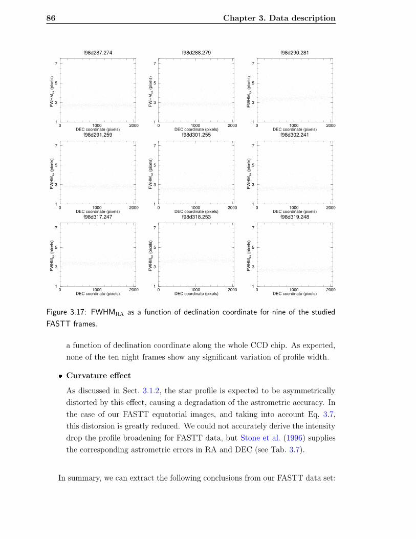
86 Chapter 3. Data description
0 1000 2000DEC coordinate (pixels)
1
3
5
7
FWHM
RA (p
ixels)
f98d287.274
0 1000 2000DEC coordinate (pixels)
1
3
5
7
FWHM
RA (p
ixels)
f98d288.279
0 1000 2000DEC coordinate (pixels)
1
3
5
7
FWHM
RA (p
ixels)
f98d290.281
0 1000 2000DEC coordinate (pixels)
1
3
5
7
FWHM
RA (p
ixels)
f98d291.259
0 1000 2000DEC coordinate (pixels)
1
3
5
7FW
HMRA
(pixe
ls)
f98d301.255
0 1000 2000DEC coordinate (pixels)
1
3
5
7
FWHM
RA (p
ixels)
f98d302.241
0 1000 2000DEC coordinate (pixels)
1
3
5
7
FWHM
RA (p
ixels)
f98d317.247
0 1000 2000DEC coordinate (pixels)
1
3
5
7
FWHM
RA (p
ixels)
f98d318.253
0 1000 2000DEC coordinate (pixels)
1
3
5
7
FWHM
RA (p
ixels)
f98d319.248
Figure 3.17: FWHMRA as a function of declination coordinate for nine of the studied
FASTT frames.
a function of declination coordinate along the whole CCD chip. As expected,
none of the ten night frames show any significant variation of profile width.
� Curvature effect
As discussed in Sect. 3.1.2, the star profile is expected to be asymmetrically
distorted by this effect, causing a degradation of the astrometric accuracy. In
the case of our FASTT equatorial images, and taking into account Eq. 3.7,
this distorsion is greatly reduced. We could not accurately derive the intensity
drop the profile broadening for FASTT data, but Stone et al. (1996) supplies
the corresponding astrometric errors in RA and DEC (see Tab. 3.7).
In summary, we can extract the following conclusions from our FASTT data set:

3.2. Data sets description 87
1. systematic errors due to drift scanning scheme in our case of equatorial data
are far smaller than those originated by other conventional sources.
2. the main error source is the seeing fluctuations.
3. FASTT shows poor CTE resulting in elongated stellar profiles in the N-S
direction and slight magnitude dependence of FWHMDEC .
4. unfortunately, we do not have quantitative calibration maps for most of the
conventional errors. For example, this is the case of focal-plane errors, CTE
or seeing fluctuations. This forced us to disregard differential astrometry with
respect to Tycho-2 catalogue (which is the usual catalogue followed in all
the meridians) and consider a multi-frame approach based on average pixel
coordinates, for obtaining an estimate of internal astrometric error instead.
This will be further explained in Sect. 4.7.
3.2.2 QUasar Equatorial Survey Team (QUEST)
The QUEST (QUasar Equatorial Survey Team) project, is a collaboration between
Yale University, the Centro de Investigaciones de Astronomıa (CIDA), the Univer-
sidad de Los Andes (ULA) and Indiana University. They designed and installed a
16×2K×2K CCDs mosaic camera at the focal plane of the 1 m Venezuelan Schmidt
Telescope. This facility has been used for surveying equatorial sky in high galactic
latitudes (∼ 4000 deg2) under drift scanning mode up to mB ∼ 21, since November
1998.
The main goal of the collaboration is to discover a large number of quasars
(∼ 104) in an homogeneous and unbiased way, which makes possible to determine
cosmological parameters through the study of the distribution of dark matter via
gravitationally lensed quasars (also known as macrolensing).
A general description of QUEST features is given in Table 3.8.
Again, as in FASTT case, drift scanning mode was chosen as the best acquisition
scheme for surveying equator in a short period of time, allowing to develop variability
studies with repeated scans of the same area.
The area of the whole array formed by the 16 2K×2K chips is 2.◦4x3.◦5. As

88 Chapter 3. Data description
Table 3.8: Generic features of QUEST telescope and camera (Baltay et al. 2002).
Location
Site Llano del Hato, Venezuela
Longitude 70◦ 52′ 0′′ W
Latitude +8◦ 47′
Elevation 3600 m
Median zenithal seeing 1.′′5
Telescope
Type Schmidt camera
Aperture 1 m
Mirror diameter 1.52 m
Focal ratio f/3
Scale 67′′mm−1
Corrector optics Field flattener lens with barrel-like distorsion
Detector
Sensor Ford-Loral CCD
Format 16x2Kx2K
Pixel size 15 µm
Average gain 1.0± 0.1 e− DN−1
Average Readout noise 13± 3 e−
FOV of single frame 34.′1x34.′1
Total effective FOV of the camera 5.4 deg2
Pixel scale 1.′′033
Observational facts
Average data throughput 3.2 Gb hr−1
Effective exposure time (δ0=0) 143s
Average seeing (FWHM) 2.4 pixels
Limiting magnitude (SNR≥10) V∼ 19.2
seen in Fig. 3.18, these are grouped in 4 four-CCDs fingers, aligned towards the
N-S direction. Each finger is covered by a color filter which resemble Johnson color
system (U,B,V and R). Therefore, the camera can collect images in each of four
colors practically in a simultaneous way.
The QUEST Schmidt telescope has its focal plane in a shape of a convex spherical
surface. To allow the CCD camera to be in a flat plane, a new 30 cm field-flattener
lens was manufactured to reimage the focal plane. The lens design includes on
purpose a barrel-like distorsion, in order to compensate the curvature effect inherent
to drift scanning mode. This was optimized for observing at zero declination.

3.2. Data sets description 89
Figure 3.18: Layout of the CCDs on the image plane of QUEST camera. Also shown
are the fingers supporting the CCDs, their pivot points, and the finger-rotating cams.
Courtesy of Baltay et al. (2002).
With QUEST data, quasar candidates can be identified by the following criteria:
1. Hα emission line survey (for 0.2 > z > 0.37) (Sabbey et al. 2001),
2. U-V vs. B-V color diagram (for z < 2.2) (Baltay et al. 2002),
3. long and short term multiband variability6 (Rengstorf et al. 2004a,b),
4. absolute proper motion.
All four are robust indicators for elaborating candidates lists, which are typically
confirmed with a posteriori spectroscopic observations at larger telescopes. In the
case of QUEST candidates, those are conducted at the 3.5 m WIYN7 telescope with
the Hydra Multiple Object Spectrograph (MOS).
By now, the variability criteria is the one which have produced larger number
of quasar candidates. Rengstorf et al. (2004a) present two preliminary samples of
248 and 203 variable candidates and claims a positive quasar detection efficiency
6Quasars are known to show intrinsic brightness variability in timescales ranging from few to
several years due to their central core nature (Ulrich et al. 1997).7The WIYN Observatory is a joint facility of the University of Wisconsin-Madison, Indiana
University, Yale University, and the National Optical Astronomy Observatory.

90 Chapter 3. Data description
of ∼ 7% in both cases. As survey progresses in area coverage and time span, the
candidate list become more and more populated.
Unfortunately, the access to WIYN or other > 3 m class telescopes is limited and
the efficiency (number of observed targets/night) which offers the MOS technique
is low compared to the candidates list increase. Therefore, recalling that the main
scope of the project is to detect macrolensing events, alternative and less time-
consuming observational techniques are required for discriminating those candidates
which show multiple components (likely to be the result of the lensed quasar) and/or
occasional visible galaxy in the vicinity of the lens. This can be accomplished by
a parallel campaign of wide field imaging observations which are being conducted
also at WIYN with the MiniMosaic camera. This instrument offers high resolution
images (0.141′′ pixel−1) under excellent seeing conditions at deep limiting magnitude
(R ∼ 23 for a 3 min. exposure).
Parallely to the quasar survey, a number of complimentary science results have
arisen from QUEST team. These range from discovery of bright TNOs (Ferrin et al.
2001), new supernova detection (Schaefer 2000, 2001; Vicente et al. 2001), discovery
of GRBs optical counterparts (Schaefer et al. 1999), survey of young low-mass and
T-Tauri stars in Orion OB1 (Briceno et al. 2001) and RR Lyrae survey (Vivas et al.
2001, 2004).
The QUEST data to be studied in this part of the thesis is divided in two
sets of nearly equatorial images. The first one corresponds to a single 568x560
pixel subframe, called q100899 F14. The second is composed of 5 256x256 pixel
overlapping frames, taken in nearly consecutive nights and which is suffixed by F13.
This data was kindly supplied by the team of QUEST collaboration at Departments
of Astronomy (van Altena et al. 2000) and Physics (Baltay et al. 2000) at Yale
University, during a research stay spent there by the author.
As shown in Table 3.9, F13 and F14 sets result from different chips: B4 and C4,
respectively. Following the chip nomenclature in Fig 3.18, B4 and C4 are located in
the same finger and follow contiguous declination strips. The V filter was used in
all the studied QUEST frames.
Both QUEST sets overlap with two MiniMosaic WIYN fields which, as explained
earlier in this section, are part of the parallel campaign devoted for discriminating
lensed quasar candidates from those previously culled via variability criteria. Fol-

3.2. Data sets description 91
Table 3.9: Specific features of QUEST-WIYN data pairs for Fields 13 and 14. Since each
QUEST set overlaps with its corresponding WIYN pair, the central coordinates (α0, δ0)
also apply for QUEST sets. Seeing for q120899 F13 is unknown.
QUEST
Frame ID Field Date Chip FWHM Filter FOV
(dd-mm-yy) (′′) (′)
q050899 F13 13 05-08-99 B4 2.0 V 4.3x4.3
q100899 F13 13 10-08-99 B4 2.3 V 4.3x4.3
q100899 F14 14 10-08-99 C4 2.4 V 9.5x9.3
q110899 F13 13 11-08-99 B4 2.2 V 4.3x4.3
q120899 F13 13 12-08-99 B4 unknown V 4.3x4.3
q180899 F13 13 18-08-99 B4 2.2 V 4.3x4.3
WIYN
Frame ID Field Date α0 δ0 Filter FOV
(dd-mm-yy) (′)
w250700 F13 13 25-07-00 19h 39m 52s −0◦ 50′ 18′′ Harris R 9.7x9.6
w240700 F14 14 24-07-00 19h 45m 42s −1◦ 30′ 24′′ Harris R 2.5x9.6
lowing the same suffix notation for the two fields, these WIYN frames will be called
w250700 F13 and w240700 F14, respectively.
The data introduced in former paragraphs are summarized in Table 3.9, and
displayed in Figs. 3.19 and 3.20 (only one night frame is shown from QUEST F13
set). WIYN images have been severely unzoomed so that they respectively match
the displayed scales of QUEST frames8. In addition, note the zoom ratio at Fig. 3.19
was chosen to be a bit smaller than in Fig. 3.20.
Systematic errors considerations
As in the case of FASTT data, we overview, and quantify when possible, those
systematic errors introduced in Sect. 3.1.1 and 3.1.2 which do apply for the QUEST
data.
A basic difference between QUEST and FASTT has to be commented at this
8Of course this causes a loss in resolution and makes visually appreciate far less stars than really
are detected by a dedicated routine.
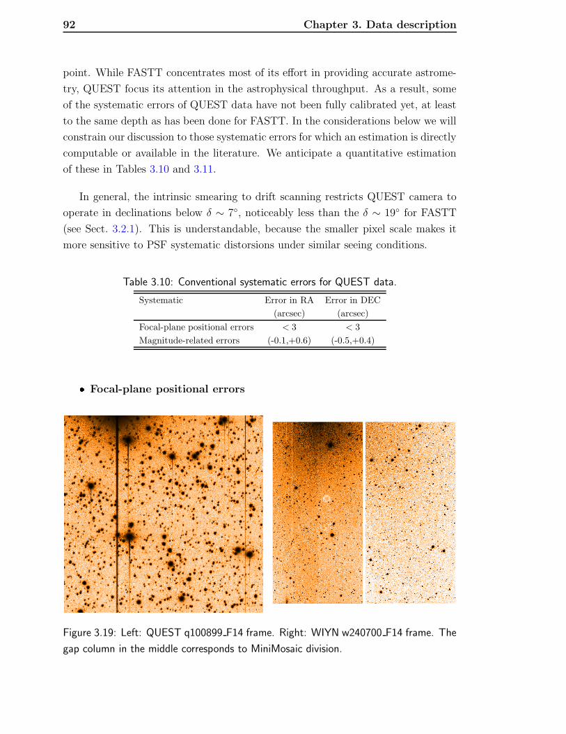
92 Chapter 3. Data description
point. While FASTT concentrates most of its effort in providing accurate astrome-
try, QUEST focus its attention in the astrophysical throughput. As a result, some
of the systematic errors of QUEST data have not been fully calibrated yet, at least
to the same depth as has been done for FASTT. In the considerations below we will
constrain our discussion to those systematic errors for which an estimation is directly
computable or available in the literature. We anticipate a quantitative estimation
of these in Tables 3.10 and 3.11.
In general, the intrinsic smearing to drift scanning restricts QUEST camera to
operate in declinations below δ ∼ 7◦, noticeably less than the δ ∼ 19◦ for FASTT
(see Sect. 3.2.1). This is understandable, because the smaller pixel scale makes it
more sensitive to PSF systematic distorsions under similar seeing conditions.
Table 3.10: Conventional systematic errors for QUEST data.
Systematic Error in RA Error in DEC
(arcsec) (arcsec)
Focal-plane positional errors < 3 < 3
Magnitude-related errors (-0.1,+0.6) (-0.5,+0.4)
� Focal-plane positional errors
Figure 3.19: Left: QUEST q100899 F14 frame. Right: WIYN w240700 F14 frame. The
gap column in the middle corresponds to MiniMosaic division.

3.2. Data sets description 93
Figure 3.20: Left: QUEST q100899 F13 frame (zoomed twice with respect to
q100899 F14 in Fig. 3.19). Right: WIYN w250700 F13 frame.
Table 3.11: Drift scanning specific systematic errors for QUEST data.
Systematic Intensity FWHM Error in RA Error in DEC
peak drop (%) broadening (%) (mas) (mas)
Discrete shifting 12 14 0 0
Differential trailing (a) (a) (a) (a)
Curvature effect (b) (b) (b) (b)
(a): Not quantified, but minimized by nearly equatorial images.
(b): Smearing below 1′′. Minimized by fingers motion and nearly equatorial images.
As stated in Pag. 88, a corrector lens with an inverse barrel-like distorsion
was inserted in front of the camera to flatten the image plane. While this is
optimal for purely equatorial observations (Baltay et al. 2002), a noticeable
focal-plane systematic error is introduced when the camera is observing at
non-zero declinations, as it is the case of our data (δ ∼ −1◦).
Abad & Vicente (2000) show that this effect is not negligible and has to be
calibrated and removed from derived astrometric positions. QUEST positions
were transformed to the reference frame defined by the Astrometric Calibration

94 Chapter 3. Data description
Regions (ACR) (Stone 1997b) in order to derive a focal-plane positional errors
map. Residuals as large as 3′′ for extreme coordinates were found.
� Magnitude-related errors
Abad & Vicente (2000) also investigated magnitude-related errors by plotting
the residuals from QUEST vs. ACR magnitude. A severe magnitude equation
was detected, both for RA and declination. Depending on the considered co-
ordinate and chip, residuals spread in the bright end (V ∼ 10−12) from −0.1′′
to +0.6′′ for RA, and from −0.5′′ to +0.4′′, for declination. Regarding inter-
mediate magnitude range and faint end, few chips showed flat trend around
zero, above all in declination.
However, it is noteworthy that raw (x, y) positions were computed by an early
version of QUEST reduction pipeline, which made use of a simple baricentre
algorithm. Therefore, this strong systematic error with magnitude is likely to
be mostly caused by the use of that inadequate centering algorithm, which
can deliver biased positions and magnitudes (Auer & van Altena 1978; Stone
1989).
� Seeing fluctuations
No specific study related to this effect has been found in the literature.
On one hand, as explained in Pag. 68, the origin of this error is totally gen-
eral and, therefore, is likely to appear in QUEST, which performs wide-field
astrometry over long periods of time. As introduced in Pag. 68, the periods of
fluctuations in the declination residuals typically range from 3-4 to 40 minutes
of time. On the other hand, the FOV of the F13 and F14 QUEST images
(see Table 3.9) is much smaller than this variation range. Therefore, again as
in FASTT case, we can assume this systematic effect will not be significant
among the rest.
� Discrete shifting
Sabbey et al. (1998) reported QUEST data to be with circularly symmetric
PSFs with FHWM∼2.′′5. In a posterior study, Baltay et al. (2002) confirm
latter measurement with the median seeing to be around 2.′′4. Both are in
accordance with the FWHM values calculated in our two data sets (see Ta-
ble 3.9). In the same article, the authors also provide 2.′′1 as the median seeing
operating in stare mode observed during the same period of time. Therefore

3.2. Data sets description 95
the overall degradation from stare to drift scanning seeings turns to be 0.′′3
(14%).
On the other hand, if we revisit Figs. 3.4 and 3.3 with the above mentioned
value of stare mode seeing (σ =0.89 pixels), we obtain a decrease in the inten-
sity peak of 12% and a profile broadening of 14%, as described in Table 3.10.
The fact that both profile broadening values coincide indicates an important
point: the rest of systematic effects due to drift scanning (differential trailing
and curvature) have been effectively minimized in the way explained in the
next two subsections.
Again, the magnitude drop due to this effect, while not being dramatic, will be
one of the reasons which justifies the convenience of the application of image
deconvolution to this kind of images.
� Differential trailing
There are three features of our data which minimize the incidence of differential
trailing over the final PSF and resulting astrometry.
First, each one of the CCDs in QUEST camera is clocked at slightly different
rates in order to compensate for the gradient in sidereal rate across the FOV.
Second, the data we are going to study belong to a single chip.
Finally, our data is nearly equatorial. As explained in Pag. 63, this turns the
differential trailing effect to be nearly null.
� Curvature effect
Two instrumental engines minimize the curvature effect impact over the QUEST
data:
As commented before in this section, the camera includes a field flattener
lens with inverse barrel-like distorsion designed to compensate the curvature
effect when observing at zero declination. It is clear that the inclusion of
this corrector is to remove the bulk of PSF smearing which the curvature
effect would introduce otherwise. However, our data has been observed at
δ = 1.5◦ instead of at the equator. To our knowledge, the implications of this
misalignment over the PSF and astrometry have not been studied in detail.
Second, as seen in Fig. 3.18 the QUEST camera include the possibility of
orientating their 4 fingers in the appropriate configuration which minimizes

96 Chapter 3. Data description
the curvature effect. Baltay et al. (2002) reports PSF smearing is kept below
1′′ thanks to this engine.
3.2.3 NESS-T: Baker-Nunn camera at Rothney Astrophys-
ical Observatory
The Rothney Astrophysical Observatory (Canada) is currently operating a wide field
Baker Nunn camera (NESS-T BNC), which has been retrofitted for CCD imagery.
This is one of wide field cameras built between 1950s and 1970s and coordinated
by Smithsonian Astrophysical Observatory for artificial satellite follow-up. Original
Baker-Nunn cameras were a modified Schmidt design with a symmetrical close triplet
group of 50 cm lenses in the entrance pupil. The focal length was 510 mm at f/1
with a workable FOV of 5◦x30◦ over the curved film field.
The NESS-T BNC was refurbished during the 2001-2003 period for enabling the
CCD observing with an automated equatorial mount (Mazur et al. 2005). Optics
were upgraded with a field-flattener corrector lens which provides a useful 4.◦4x4.◦4
FOV for the 4K×4K chip installed at prime focus.
A general description of the NESS-T BNC features is given in Table 3.12. For a
closer understanding of the instrumental aspects of this facility, we refer the reader
to Appendix A, where a very similar project, operated by Fabra Observatory and
Real Instituto y Observatorio de la Armada en San Fernando, is presented.
One of the main programs developed in this telescope is called Near-Earth Space
Surveillance Terrestrial (NESS-T) and aims to provide a new census of NEOs in
North pole regions where other instruments located in moderated latitudes cannot
access. NESS-T is the facility with widest FOV specifically dedicated to professional
asteroid search. Note that NESS-T is optimized for NEOs discovery, and not for
accurate astrometry. In this context, the project is fully operative in the detection
part, but a complete astrometric calibration is still being held.
The data set considered in this section was kindly supplied by the NESS-T team
at Rothney Observatory and Department of Geology and Geophysics at University
of Calgary (Hildebrand et al. 2004). This study is inscribed in a wider collaboration
for optimizing the scientific return of the two BNCs (NESS-T’s and the one in San
Fernando), and has been recently complemented with research stay of a member

3.2. Data sets description 97
Table 3.12: Generic features of NESS-T Baker Nunn camera.
Location
Site Rothney Observatory, Calgary (Canada)
Longitude 114◦ 17′ 18′′ W
Latitude +50◦ 52′
Elevation 1284 m
Telescope
Type Modified Schmidt camera
Aperture of corrector triplet lens 0.5 m
Mirror diameter 0.78 m
Focal ratio f/1
Scale 410′′mm−1
Corrector optics 2-element Field flattener lens
Spot size 20 µm
Filters Light Pollution Removal (LPR) 99% (710± 210nm)
Detector
Sensor Kodak KAF-168801E
Format 4Kx4K, 9 µm, 36.8mmx36.8mm
QE 67% (peak)
Camera Finger Lakes Instrumentation IMGX16801E
Average gain 1.73 e− DN−1
Average Readout noise 14.41 e−
Pixel scale 3.′′9
CCD FOV 4.◦4x4.◦4
Cooling Peltier (∆T ∼ 50 Õ )
Support CCD Spider with low expansion material and
±1 µm accurate remote focus
Observational facts
Acquisition mode Stare
Typical exposure times 30s-180s
Limiting magnitude (IT=120s and SNR=1.3) V∼ 19.2
of our group, Maite Merino. The data features of this set do not correspond to
habitual near pole NEOs observational strategy, but a test data customized for this
deconvolution study.
As shown in Table 3.13, this particular set of NESS-T data comprise 10 over-
lapping frames taken in the same night. All these 30s exposures were conducted
under stare mode during a short interval of time (1 hour). Seeing for that night was

98 Chapter 3. Data description
Table 3.13: Description of NESS-T data to be studied.
Night global features
Seeing ∼ 3′′
FWHM 2.1 pixels
Filter LPR
Considered FOV Central patch of 0.◦8x0.◦8
Exposure time 30s
α0 17h 45m 26s
δ0 +39◦ 21′ 42′′
Frame specific features
Frame ID Date Time
(dd-mm-yy) (hh:mm:ss)
NESS-T 01 12-11-04 03:37:49
NESS-T 02 12-11-04 03:44:00
NESS-T 03 12-11-04 03:50:11
NESS-T 04 12-11-04 03:56:23
NESS-T 05 12-11-04 04:02:36
NESS-T 06 12-11-04 04:08:45
NESS-T 07 12-11-04 04:14:57
NESS-T 08 12-11-04 04:21:16
NESS-T 09 12-11-04 04:27:27
NESS-T 10 12-11-04 04:33:37
significantly worse to the average in that site.
By the time the observations and data analysis were conducted, no precise dark
and flatfield calibration frames were available. The implications of this oer the
results will be discussed in Sects. 5.3.2 and 5.4.2.
Although unsuccesfully, an effort for obtaining realistic flatfield calibration frames
was performed. Note that accomplishing this in an f/1 system is not straighforward.
The usual techniques employed in slower telescopes are not valid in this case. On one
hand, the usual twilight exposures do not suffice because of the significant brightness
gradient within the large FOV of the BNC. On the other hand, dome flats suffer from
appreciable stray and off-axis light which unvalidate the assumption of a uniformly
illuminated source. Finally, with such a fast system as this, very short exposure
time are required and, as a result shutter mapping correction becomes appreciable.

3.2. Data sets description 99
1 2 3 4 5FWHM (pixels)0
50
100
150
200
NESS−T_01
1 2 3 4 5FWHM (pixels)0
50
100
150
200
NESS−T_02
1 2 3 4 5FWHM (pixels)0
50
100
150
200
NESS−T_03
1 2 3 4 5FWHM (pixels)0
50
100
150
200
NESS−T_04
1 2 3 4 5FWHM (pixels)0
50
100
150
200
NESS−T_05
1 2 3 4 5FWHM (pixels)0
50
100
150
200
NESS−T_06
1 2 3 4 5FWHM (pixels)0
50
100
150
200
NESS−T_07
1 2 3 4 5FWHM (pixels)0
50
100
150
200
NESS−T_08
1 2 3 4 5FWHM (pixels)0
50
100
150
200
NESS−T_09
Figure 3.21: Histograms of FWHM for nine of the 11 studied NESS-T frames. FWHM
values were obtained by profile 2D Gaussian fitting.
All previous complications were confirmed by observation tests taken by Merino
(2004), and it has led us to the convenience of exploring other flatfield techniques,
still to be tested. As a result, only the central 1K×1K subframe of 0.◦8x0.◦8 FOV
was considered (see Fig. 3.22), where the flatfield and vignetting contributions are
reasonably negligible. This election will allow us a more direct understanding of the
benefits introduced by image deconvolution. With identic purpose a region lacking
stellar crowding and very bright stars was chosen. A light pollution removal (LPR)
filter was used for skipping sodium lamps emission present in suburban skies like
this. As mentioned above, NESS-T is mainly dedicated to NEOs discovery, and not
to accurate photometry. Therefore, as to maximize photon gathering is the main
concern the choice of LPR filter is fully justified.

100 Chapter 3. Data description
As can be seen in Fig. 3.21, sampling of NESS-T frames is comprised between
2.1 and 2.5 pixels. In contrast to most telescopes, the main contributor to FWHM is
the spot size of the optical system, which on average accounts for rms∼ 20µm (∼ 2.2
pixels) over the CCD FOV. From the observation logs of that night seeing is known
to be about 3′′ due to the presence of thin clouds and moderate wind. In this regime,
the seeing contribution (∼0.7 pixels) to final FWHM matches well the second order
variations in the histogram peaks in Fig. 3.21. In conclusion, the sampling (FWHM)
of stellar profiles in NESS-T images is mostly dominated by the optical spot size
and the slight modulation due to atmospheric seeing is only significant with quite
bad seeing conditions (≥3′′). Apart from the fact that NESS-T was not taken under
drift scanning, three important differences come up when comparing NESS-T to
FASTT data. First, NESS-T PSF is slightly correlated with seeing and dominated
by optical spot size and its systematic distortions over the FOV. Second, as a result
of its coarser pixel scale (3.9′′pixel−1), NESS-T data are likely to show significantly
larger object blending than in FASTT case. Finally, note that NESS-T sampling is
closer to the critical sampling limit (FWHM=2.0 pixels) for a Gaussian profile than
FASTT’s. All three differences will have consequences in the results and analysis of
NESS-T deconvolved images, discussed in Sects. 5.3.2 and 5.4.2.
Systematic errors considerations
In contrast to FASTT and QUEST cases, systematic errors only related to stare
mode (introduced in Sect. 3.1.1) do apply for NESS-T data.
Being NESS-T an observational program with recent first light, few systematic
errors have been definitively calibrated. However, the most important errors (sum-
marized in Table 3.14) have been already identified and are roughly discussed below.
� Focal-plane positional errors
Although no map of focal-plane positional errors is available, several consid-
erations on behalf of this can be addressed.
First, we recall that in its original design, the focal plane of the BNC was
spherical. Thanks to the inclusion of a 2-element lens field flattener corrector
and a proper collimation of the system the focal plane has turned out to be
practically flat within the CCD FOV.

3.2. Data sets description 101
Figure 3.22: One of the 1K×1K (0.◦8x0.◦8 FOV) CCD frames from NESS-T Baker Nunn
camera to be studied. The stellar density is sparse enough for avoiding undesirable
crowding effects. The presence of very bright stars and its associated blooming is also
minimized.
Second, and despite the former, when performing plate astrometric solution of
our NESS-T frames, high order polynomials have been required to fit the whole
FOV to standard astrometric coordinates using USNO-A2.0 (Monet et al.
1998) as reference catalogue. After this plate correction a significant number
of star residuals exceeded far more than 3 times the rms of the fit (0.′′25). Of
course, this experiment is not conclusive and should be repeated with more
denser grid of reference stars spread all along the CCD array and more accurate

102 Chapter 3. Data description
Table 3.14: Most important systematic errors for NESS-T data.
Systematic Error in RA Error in δ
(arcsec) (arcsec)
Focal-plane positional errors > 1 > 1
Systematic Intensity FWHM Error in RA Error in δ
peak drop (%) broadening (%) (mas) (mas)
Pixel response function ∼ 3% ∼ 2% 0 0
reference catalogue (for example UCAC2 (Zacharias et al. 2004b)). However,
it is already indicative that the systematic focal-plane positional errors do
exist in NESS-T camera and they are above the typical astrometric accuracy
supplied by the camera.
Finally, it has been observed that the NESS-T PSF does show appreciable
variability across the whole 4.◦4x4.◦4 CCD FOV. However, this effect becomes
minimized in the central 0.◦8x0.◦8 patch considered for this study. In addition,
as will be shown in Sect. 5.1.3, NESS-T PSF suffers from coma even in this
central patch. It is noteworthy that posterior recollimations of the optical
system have been performed in order to improve PSF uniformity.
On the whole, it is noteworthy that, luckily, our data set was acquired in a very
homogeneous fashion. In other words, the objects coordinates derived from
our 10 frames practically overlap (there are no inter-frame offsets) and, as the
astrometric accuracy will derived just by the comparison of pixel coordinates
of every frame (see Sect. 4.7), the positional systematic errors do not play a
decisive role in our case.
� Pixel response
Despite the relatively coarse scale of NESS-T images, the fact that the sam-
pling is dominated by spot size up to a level always well above FWHM=2′′
leads to that the broadening of stellar profile due to pixel response function
is not as crucial as in drift scanning images as FASTT and QUEST. For a
typical sampling value of σ = 1.0 pixels, which is very close to the FWHMs
shown in Fig. 3.21, an intensity drop of 3% and a FWHM broadening of 2%
were derived from Figs. 3.4 and 3.5.
� Seeing fluctuations

3.2. Data sets description 103
Although we do not have any study of this systematic error in NESS-T data,
we do not expect it to be of decisive importance over the derived astrometry.
This is because, as we mentioned above, NESS-T PSF is mostly determined
by the spot size diagram of the optical system and not by atmospheric and its
associated temporal variations.
� Photon shot noise
The number of incoming background photons are proportional to the pixel
area. In the case of NESS-T pixel, this is 7 (15) times larger than FASTT’s
(QUEST’s). In addition, NESS-T sky is not as dark as FASTT’s or QUEST’s.
As a result of these two factors, NESS-T background noise is dominated by
Poissonian statistics at early exposure times (e.g. 30s)9. This translates into
a lower SNR for a fixed exposure time, or equivalently, an decrease of the
limiting magnitude of the image.
Attending this, we will show in Sects. 5.3.2 that AWMLE deconvolution can
be considered as solution for compensating that loss of limiting magnitude.
� Vignetting obscuration
This particular data set suffers from significant vignetting. This was due to
the excessive shutter diafragming which was installed to remove lateral light.
As a result, about 6% of flux variation between the centre and the edge of the
FOV was observed in our data. That problem was overcome by considering
only the central patch of 0.◦8x0.◦8, where such effect is minimized. That shutter
diafragming problem was solved after this study was completed.
9Note that at this high count regime, Poissonian probability distribution can be approximated
by a Gaussian with a dispersion of σ =√n, with n the number of counts.

104 Chapter 3. Data description

Chapter 4
Proposed methodology
In this chapter we describe the methodology proposed for applying deconvolution
to CCD images of arbitrary properties. Two separate stages in this reduction pro-
cess are distinguished. First, the one devoted to calibrate and characterize the
original data set for preparing the deconvolution. A diagram of the whole proce-
dure is shown in Fig. 4.1. Second, the one dedicated to assess the deconvolution
performance in terms of limiting magnitude gain, limiting resolution gain and as-
trometric precision. Each one is composed of several steps, namely: generic CCD
reduction (Sect. 4.1) and PSF fitting (Sect. 4.2) for the first stage, and object detec-
tion (Sect. 4.3), limiting magnitude gain calculation (Sect. 4.4), limiting resolution
gain calculation (Sect. 4.5), source centering (Sect. 4.6) and astrometric precision
estimation (Sect. 4.7) for the second stage.
4.1 Generic CCD reduction
As justified in Chapt. 2, image deconvolution requires an accurate description of all
the uncertainties presented in the data.
In CCDs, that begins with the knowledge of fundamental aspects of the data as
the amplifier gain, readout and dark current noises and spatial quantum efficiency
variations along the detector. This generic calibration turns to be the first step for
whatever analysis algorithm. Image deconvolution is not an exception, as the proper
removal of all these effects allows to separate the measured image pj from flatfield
105

106 Chapter 4. Proposed methodology
Calibrated image
CCD parameters(gain, readout noise)
IRAF.daophotPSF fitting Background estimation
SExtractor
Raw image
Deconvolution
PSF image
Deconvolved image
Background image
(bias,dark,flatfield)IRAF.ccdred
CCD generic reduction
MLE or AWMLE
Figure 4.1: Flow-chart of the methodology for pre-deconvolution reduction steps. Back-
ground estimation is explained in Sect. 4.3, as part of the object detection process.
Cj and background bj maps, which are input parameters of MLE and AWMLE
deconvolution algorithms.
At this point, an important remark arise from Eq. 2.1. While Cj contributes
multiplicatively to the measured data, bj is an additive term. As a result, the cor-
rect assignment of every single signal ADU to either Cj or bj is crucial for posterior
image deconvolution performance, since this aims to keep original statistics and it
distinguishes between flatfield (multiplicative) and background (subtractive) con-
tributions. Therefore, both Cj and bj should be estimated with the best accuracy
possible.
For the case of CCD data taken under stare mode this generic reduction needs
to have bias, dark and flat calibration frames. The procedure is very well-known
and has been implemented in most astronomical reduction packages, as for example
ccdred package (Valdes 1988) inside IRAF.
However, this generic calibration is not so well established for the case of drift
scanning data, at least for the flatfield correction. As introduced in Sect. 3.1.2, this
acquisition scheme naturally flatfields the resulting image, as each sky elementary
region is sampled by every pixel in a row. Consequently, a certain pixel has an
spectral response which is the mean quantum efficiency of all the pixels in its row.
As a result, pixel-to-pixel noise is diminished. This is why some surveys do not apply

4.2. PSF fitting 107
flatfield correction to their scanning strips. Others extract a flatfield vector from
object frames themselves by calculating, for all the rows in the image, the mode of
all pixels along a given row (Richmond et al. 2000). This special flatfield technique
was implemented as a custom script inside IRAF.
4.2 PSF fitting
PSF fitting has been one of the mainstream topics in data analysis in astronomy
during the last decades. It was originally motivated by the need of performing
precise photometry in crowded fields. As a by product of this effort a kernel of the
PSF can be obtained and introduced in the methodology we are defining as an input
parameter of image deconvolution algorithm (see Fig. 4.1).
The performance of image deconvolution is highly dependent of the accuracy of
the PSF modelling. Among other effects, an occasional deviation of the model with
respect to the actual PSF can result in the confusion of those faint sources which
are disposed around brightest stars. As MLE-family deconvolution algorithms are
iterative, this mismatch incorporated in the PSF modelling can yield to undesirable
artifacts in the solution image. Ideally, errors caused by uncertainties in the PSF
should be well below noise fluctuations.
As anticipated in Sect. 1.1, the shape of telescopic PSF has been the subject of
a number of studies. For the case of ground-based astronomy, both in photographic
plates (King 1971) and in CCDs (Racine 1996) the authors define two well-separated
parts in the PSF profile. These have different origin and localization on radial
distance to the center θ:
� a central core caused by atmospheric turbulence. A number of factors, as the
changes in wind speed and direction, index refraction and density play a key
role in the magnitude of this turbulence. The larger the turbulence the broader
this profile is. Note that this part of the PSF (commonly denominated as Kol-
mogorov profile or simply seeing) is slightly dependent (∝ λ65 ) on wavelength
(in optical and IR) (Racine 1996). As a result of the stochastic nature of this
component, its shape cannot exactly be described in analytical means. Two
profiles have been proposed in the literature for accounting this distorsion.

108 Chapter 4. Proposed methodology
First, a Gaussian shape (Lagendijk & Biemond 1991) which is a simple model
and convenient because of its particular properties in the Fourier space. (Stet-
son 1992, 1994) has also proposed 2D elliptical Gaussian model, which adds
more flexibility for elongated profiles.
Second, Moffat (1969) first introduced and gave name to a radially symmetric
function which can be expressed as:
I(θ) =I0
(
1 + θ2
R2
)β(4.1)
where R is related to FWHM by FWHM = 2R√
21/β − 1 and β is a parameter
which measures the power of the wings at large θ’s. This function has been
found to fit the Kolmogorov profile better than the Gaussian profile, specially
in the outer part up to θ ∼ 5 FWHM, where Gaussian profile decays faster
than Moffat (Racine 1996).
Eq. 4.1 has also been used for fitting space-based PSFs which showed extended
emission in the outer wings, even above the power defined by Moffat function.
This was the case of aberrated pre-COSTAR HST PSF, whose best analytical
fit responds to that expression with β=1, also called Lorentzian function.
In the limit of β = 0, the Moffat function of Eq 4.1 becomes a radially sym-
metric Gaussian.
� an extended external aureole with a decreasing intensity as the inverse square
of the radial distance. This component becomes dominant over the central
core for θ > 5 FWHM (turbulence limit). It is caused by a combination
of atmospheric and instrumental effects. First, the optical system may have
aberrations or anomalies. Depending on the their strength, the outer structure
might be complex and even show asymmetries (e.g. coma). Second, the light
is scattered by atmospheric aerosols, scratches or dust on telescope optics. Fi-
nally, the diffused and reflected light in the detector assembly also contributes
to this outer halo.
Note that the magnitude difference between the peak of the central core and
the region where aureole begins to become dominant (θ ∼ 5 FWHM) is about 11-
12 mag (Racine 1996). Taking into account that this magnitude range nearly fulfills
the whole CCD dynamic range and that background level in wide field surveys is
usually high, it can be concluded that aureole will not be really appreciable in bright

4.2. PSF fitting 109
non-saturated stars. In the brightest saturated objects some information of this PSF
component could be extracted, but only in basis of a reduced sample of elements.
Therefore, apart from a few state-of-the-art experiments of PSF characterization
or very exotic data which may use saturated stars wings, the rest of ground-based
PSF fitting work has been devoted to model the Kolmogorov profile dominated by
turbulence. In addition, in the case of undersampled data, an attempt of fitting
aureole features from saturated stars could be in danger of recovering part of the
high frequency smearing introduced by aliasing. In accordance to this, we will
concentrate the subsequent PSF analysis within turbulence limit radial distance
(θ < 5 FWHM).
Most of PSF fitting packages have Gaussian and Moffat profile functions as
models choices (Buonanno et al. 1983; Mateo & Schechter 1989; Penny & Dickens
1986). This is also the case of the reduction tool considered for our PSF modeling,
DAOPHOT II1 (Stetson 1992; Stetson et al. 1990), which has the following ones:
1. a Gaussian function,
2. a Lorentzian function, as defined in Eq. 4.1 with β = 1,
3. two Moffat functions, as defined in Eq. 4.1 with β = 1.5 and β = 2.5.
For all three models DAOPHOT II includes additional 2D elliptical parameters which
allow to reproduce elongated profiles. An interesting feature which is not available
in DAOPHOT II would have been to have a PSF model composed by the combination
of two Moffat analytical functions. In theory, this is the model (with β = 7 and
β = 2) which best fits Kolmogorov profile (Racine 1996).
It is not in the scope of this thesis to review the procedure followed by DAOPHOT
II for fitting the PSF. In brief, it consists in an iterative process which numeri-
cally computes the PSF by fitting a list of selected stars to a specified model with
weighted least-squares method. Every iteration step includes removal of close neigh-
bours from selected stars sample. This fitting procedure is interrupted when either
a satisfactory data-model rms deviation is achieved or the maximum number of al-
lowed iterations is reached. We refer the reader to Davis (1994); Stetson (1987) for a
complete description. However, in the following some considerations about DAOPHOT
II procedure which are pertinent for our deconvolution application are outlined:
1It is included in standard IRAF distribution

110 Chapter 4. Proposed methodology
1. largely discordant pixels, mostly caused by cosmic rays and overlapping with
neighbour stars, are automatically penalized in the fitting process. These are
identified by comparing among those pixels located at the same place within
the profiles of the other selected stars.
2. in principle, this new version of the package offers the possibility of including
saturated stars in the derivation of the final PSF. As stated above, the outer
regions of these objects yield information about the aureole component of the
PSF. After several tests, we concluded that the inclusion of saturated stars
in the PSF model does not lead to significant improvements, at least for the
data presented in Chapt. 3. We attribute this to the fact of disposing of a few
(sometimes only one) saturated star in the studied FOV.
3. in general, the whole PSF fitting process can be automated. In our specific
case, still some visual inspection and catalogue identification of the PSF se-
lected stars was performed by the author, for discarding close blending or
extended objects (galaxies). However, this interactive step was found to be
irrelevant most times, and could be easily protocolized for its complete au-
tomation. Note this is very convenient for the overall integration of the de-
convolution algorithm in a unattended reduction pipeline.
4. the purely analytical fitting approach has been found insufficient for com-
pletely modeling the PSF. Normally, analytical function can reproduce up to
95% of the intensity variations within a star’s profile (Stetson 1992). The re-
maining 5% residual is mainly distributed in the outer wings before reaching
the turbulence limit (3 < θ < 5 FWHM). In response to this, DAOPHOT II
offers the possibility of using an empirical look-up table of correcting values in
order to mitigate this fitting deviation. As a result, the photometric scatter is
significantly improved even for undersampled data.
Note that this part of the stellar profile is the one more affected by background
noise. Therefore, the solely incorporation of this correction table by averag-
ing pixel values of selected targets could imply the undesired introduction of
high frequencies features related to noise and aliasing. This problem can be
mitigated by sampling residuals at higher spatial resolutions than the obser-
vational data. In the case of DAOPHOT II, these are oversampled in grid twice
finer by using bicubic interpolation.
As explained in Sect. 2.1.2, the fact that the detector is composed by finite pixels

4.2. PSF fitting 111
introduces an additional distorsion in the PSF when this is sampled in the detection
process. As the pixel size increases with respect to PSF width (lower FWHM), more
and more flux is localized in the few central pixels. Interesting experiments about
DAOPHOT II performance in different data sampling regimes have been carried out
by Stetson et al. (1990) with real images. Table 4.1 includes a summary of results
for the same set of real (non-synthetic) stars, spanning a wide magnitude range,
in oversampled and severely undersampled conditions. From the inspection of the
table several considerations arise:
Table 4.1: Sampling-induced photometric scatter (Stetson et al. 1990).
PSF Model σ (mag)
FWHM = 2.54
Gaussian+LUT(a) 0.0077
Moffat+LUT 0.0081
FWHM = 0.85
Gaussian 0.0894
Gaussian+LUT 0.0826
Moffat 0.0281
Moffat+LUT 0.0178
(a) Empirical look-up table of correcting values.
� Gaussian and Moffat models seems to be equally preferable for the oversampled
case despite the theoretical priority for Moffat justified above.
� σ is in general worse for the undersampled case. This scatter increase is
induced by the interpolation method used to encode the PSF.
� the case of Gaussian model is specially hampering in the undersampled case
and denotes the poor performance of this model under these sampling con-
ditions. This discrepancy is not only localized in the outer wings, but also
in the central pixel of the profile. The latter is justified by the fact that the
inclusion of the look-up table (which is mainly defined in outer wings) over
the Gaussian model does not lead to a great improvement.
� Moffat model shows a remarkably better performance for undersampled data.
Therefore, again as the Kolmogorov profile reasoning, Moffat profile is favoured

112 Chapter 4. Proposed methodology
in place of Gaussian function because it is less affected by sampling-induced
interpolation errors of PSF fitting packages.
� with the addition of a look-up table of corrections, Moffat scatter is slightly
improved and approaches to the figure of over-sampled data.
In summary, photometric scatter derived from DAOPHOT II seriously degrades with
undersampling for Gaussian model, but this is nearly avoided if Moffat model is
considered.
Note the discussion above was dealt around photometric, not astrometric, scat-
ter. The latter will be issued in Sect. 4.6.
4.3 Object detection
The object detection process is conducted with SExtractor (Bertin & Arnouts
1996). This package is widely used among the astronomical community, and has
shown to be a robust tool in a large variety of data features (CCD and photographic
response, sampling, SNR, etc.).
The algorithm followed by SExtractor can be divided in four separated phases:
1. the sky background (either constant or variable across the field) is modeled by
using a combination of κσ-clipping and mode estimation.
2. the image is background-subtracted, filtered and thresholded. As the fil-
tering process, this is performed via a convolution with an optimal kernel
(FILTER NAME) which matches the PSF of the image. This particular choice
maximizes the detectability. In our particular case, we chose FILTER NAME
to be a Gaussian kernel with FWHM close to the PSF one. One might ob-
ject that to use the same convolution kernel is not appropriate because PSF
is indeed variable across the image. However, detectability has been found
to be a rather slow function of the FWHM of employed kernel (Irwin 1985).
For example, a mismatch of 50% between the kernel FWHM and that of the
PSF, which is far larger than what we expect from typical PSF variations in
our data, leads to no more than a 10% loss in SNR peak. A similar test of

4.3. Object detection 113
this trend was performed for both original and deconvolved QUEST images
(Sect. 3.2.2), yielding to even smaller loss of detection efficiency.
Two key parameters play an important role in the thresholding step. First,
DETECT THRESH which is the detection threshold, in units of background rms
(σ)2. And second, DETECT MINAREA which is the minimum number of 8-
connected3 pixels above threshold for a positive detection.
Finally, a flag image FLAG IMAGE can be used to specify those regions in the
image likely to trigger false detections due to dark and hot pixels, deferred
charge columns, CCD defects, etc. These detections are accordingly flagged
for later disregarding.
3. a deblending process is run over the detection list obtained in step 2. The pixels
of each thresholded object are filtered in order to obtain occasional overlap-
ping components. This filter is based on a multi-thresholding technique which
does not make any assumption about the object profile. Its performance is
modulated by DEBLEND MINCONT parameter. This is the minimum deblending
contrast and establishes how sensitive is SExtractor to blended objects. Of
course, this parameter is crucial for resolution gain study described in Sect. 4.5.
4. photometry and classification via image segmentation are performed for all
the detected objects, before writing to the output catalogue to disk.
Optimal values for the above key parameters were found after some empirical
learning in each data set, for both the original and deconvolved images. This param-
eter tuning does not lead to the same values depending the purpose. For example,
narrower FWHM values for FILTER NAME were found to be more effective in the
resolution gain study (Sect. 4.5) than the ones employed in the limiting magnitude
study (Sect. 4.4), although that choice imply a slight increase of false detections in
the former case.
2Note that SNR is proportional (not identical) to DETECT THRESH. For example, Benıtez et al.
(2004) found in the context of galaxies detection that SNR=3.5 when DETECT THRESH=1.5.3Two pixels are 8-connected if their edges or corners touch.

114 Chapter 4. Proposed methodology
Catalog listresolution image
Deep highDepurateddetections
Object detectionSExtractor
Deconvolved image
Limiting magnitudegain calculation
Catalog
Calibrated image
Raw detections listRaw detections list
SExtractor
Detections validation
Validated detections listwith external photometry with external photometry
Validated detections list
Deep and high resolution image validationAstrometric catalog validation
pixel reference frameTransformation to
Object detection
∆m
(xcat, ycat) (xhr, yhr)(α, δ)
(xdecon, ydecon)(xorig, yorig)
(xvaldecon, y
valdecon)(xval
orig, yvalorig)
Figure 4.2: Flow-chart of the methodology for post-deconvolution reduction stages. The
validation of raw detection lists can be derived from either astrometric catalogue (left)
or deeper and higher resolution image (right). Multiframe comparison validation process
has not been included as it was not finally used.
4.4 Increase in SNR and limiting magnitude
The aim of this Section is to define a methodology for validating the detections
found by SExtractor in the former Section. Once these have been assured to be
true with one of the procedure proposed in Sects. 4.4.1, 4.4.2 and 4.4.3, and not due
to artifacts, they can be used for calculating the limiting magnitude gain introduced
by deconvolution. The diagram shown in Fig. 4.2 summarizes the steps involved in
this process.
Typically, for multiframe CCD data sets as the ones described in Sect. 3.2, we
propose three alternatives in order of preference which we describe in the following.

4.4. Increase in SNR and limiting magnitude 115
4.4.1 Validation with a deeper and higher resolution image
Wide field surveys normally conduct follow-up observations with larger telescopes
when confirmation is needed for a number of selected objects. Therefore, a deeper
and higher resolution image which overlaps the selected survey image might be
available in some cases. In addition, it is preferable that both images have been taken
with similar bandpass filters. This should ease the confirmation of faint detections
which might not appear in deeper image because of extreme spectral types.
The followed methodology is simple. First, SExtractor detection is performed
in both survey and deeper images. Next, the latter detection list in pixel coordinates
is transformed to the pixel reference frame of the former one, by using xyxymatch,
ccmap and cctran tasks inside IRAF. Finally, a matching process is performed keep-
ing those objects in common (within a tolerance radius) between the survey and the
deep images lists.
4.4.2 Validation with reference catalogue
All-sky deep and accurate astrometric catalogues have become common along the
last decade. As seen in Tab. 4.2, in most cases (with the exception of UCAC2) their
limiting magnitude is large enough for assuring object completeness for moderately
deep images (Vlim < 20), as the ones we study in this part of the thesis (see Sect. 3.2).
USNO-B1.0 and GSC 2.2 would be the more appropriate choices, since provide high
stellar density, acceptable astrometric error and proper motion information. USNO-
A2.0, although it shows about half number of objects than USNO-B1.0 and does
not provide proper motions, is still a reasonable alternative for the level of accuracy
required for our limiting magnitude gain study.
Note that recent efforts for merging best astrometric and photometric catalogues
available (HIPPARCOS, Tycho-2, UCAC2, and USNO-B) have led to the release of
NOMAD (Zacharias et al. 2004a). Although NOMAD provides the best astrometric
and photometric data for a given star, our concern to keep homogeneity in the
magnitude scale made us to disregard this alternative and keep USNO-B1.0 as the
reference catalogue despite its considerable poor photometric error.
Catalogues are queried online with the scat program of WCSTools package (Mink

116 Chapter 4. Proposed methodology
2002). Next, (α,δ) coordinates are transformed to the pixel reference frame by using
ccxymatch, ccmap and cctran tasks inside IRAF. Finally, a matching process is
performed keeping only those objects common to the frame detection list and the
catalogue within a tolerance radius.
Table 4.2: Overview of some all-sky astrometric catalogues.
Name Number Limiting Mean error Reference
of objects magnitude (at J2000)
UCAC2 48,330,571 R ∼ 16 0.′′015–0.′′070 (Zacharias et al. 2004b)
GSC 2.2 435,457,355 J ∼ 19.5 0.′′3–0.′′75 (Morrison et al. 2001)
USNO-A2.0 526,280,881 V & 20 0.′′25 (Monet et al. 1998)
USNO-B1.0 1,045,913,669 V ∼ 21.0 0.′′2 (Monet et al. 2003)
4.4.3 Validation with multiframe comparison
One of the survey frames is considered as reference. Next, the rest of detection lists
are transformed into this reference system. Finally, a matching process is performed
keeping only those objects appearing in all lists, within a tolerance radius.
For the matching process used in all three methodologies described in Sects. 4.4.1, 4.4.2
and 4.4.3 a tolerance radius value needs to fixed. There are several factors which con-
strain the optimum value of this parameter. On one hand, in the case of Sect. 4.4.2.,
the mean random error of the reference catalogue can contribute to slightly enlarge
the residual between the pixel coordinates of survey and catalogue lists. The im-
pact of high proper motion objects with respect to their position in the reference
catalogue has been found non significant for the statistical nature of the limiting
magnitude study4. On the other hand, if the tolerance radius is too large it could
lead to fictitious detections due to neighbouring objects contamination. In conclu-
sion, the value for the tolerance radius will be empirically determined attending the
above mentioned constrains for each particular data set. This value will be assigned
4Note that, given the pixel scales of the data sets in Sect. 3.2 (1′′–4′′), even the highest proper
motion objects would need epoch difference larger than the ones found in catalogues of Tab. 4.2
for producing wrong validations. Anyway, if present, a very small number of objects would be
affected, and would not yield to biased estimations of limiting magnitude gain.

4.4. Increase in SNR and limiting magnitude 117
to the ASSOC RADIUS parameter in SExtractor, which will accordingly perform the
matching process between the survey and reference lists.
Several reasons justify the preference order of the three validation methodologies
exposed above:
� First, if the follow-up image in Sect. 4.4.1 is deep enough (2–3 additional
magnitudes), this is very likely to include all the objects detected in the survey
image. In contrast, the degree of completeness achieved in Sect. 4.4.3. is
subordinated to the number of detections offered by the frame with worst
seeing. This can yield to an effective underestimation of limiting magnitude
gain achieved by deconvolution.
� Second, although the use of a deep reference catalogue as Sect. 4.4.2 (e.g. USNO-
B1.0) could offer completeness even for the list of deconvolved images, their
performance in front of blended objects is not so optimal as the follow-up image
in Sect. 4.4.1, which can have far better resolution5. In addition, occasional
mismatches due to proper motion in Sect. 4.4.1 would be marginal, given the
very short epoch difference between our survey and follow-up images.
� Third, both follow-up images of Sect. 4.4.1 and reference catalogues of Sect. 4.4.2
include false objects. The former due to image artifacts (cosmic rays, deferred
charge columns and hot and cold pixels). The latter due to plate internal
reflections, emulsion defects, etc. However, while the former can be easily
removed by either visual inspection6 or filtering detection parameters (ellip-
ticity, roundness), the latter are usually undetectable, since catalogues do not
provide such kind of morphology information.
� Finally, as commented above, most references catalogues in Tab. 4.2 are pho-
tographic plate based. In this situation, missing objects around very bright
stars are common.
After one of the three validation methodologies is chosen attending for each data
set, this is applied to both the original and deconvolved image. As a result, the
values for number of raw (N raw), matched (Nmatched) and unmatched (Nunmatched)
5Note that all deep catalogue in Tab. 4.2 were compiled from photographic plates with a 0.′′8–1′′
pixel scale.6At least for demostrative examples like the ones of this thesis.

118 Chapter 4. Proposed methodology
detections are obtained for each image. Raw detections are simply those being
output by SExtractor. Matched detections are those raw detections (from original
and deconvolved images) which are present in the reference list, in accordance to
the validation method chosen. On the contrary, unmatched detections are those
which are not present in reference list. The latter and their origin will be separately
discussed for each data set. For a given deconvolution algorithm, a large increase in
Nmatched is as important as the control of a low Nunmatched.
The ratio of Nmatchedorig to Nmatched
deconv is a direct indicator of the limiting magnitude
gain. This can be written as:
∆m = mdeconv −morig = 2.5 logNmatched
deconv
Nmatchedorig
(4.2)
The result led by Eq. 4.2 is similar to that derived from dividing the areas below
the magnitude histograms of matched objects for both original and deconvolved
images.
Complementary, other descriptors can be considered for understanding the way
image deconvolution improves limiting magnitude. They are the number of detec-
tions (raw and matched) versus number of iterations, the number of detections (raw
and matched) versus detection threshold and the magnitude histogram of matched
detections versus number of iterations. They all will be used in Sects. 5.3.1 and 5.3.2
for the considered data sets.
4.5 Increase in limiting resolution
The aim of this Section is to define a methodology for estimating the gain in limiting
resolution delivered by image deconvolution.
A simple custom program was developed for pairing all the objects with their
closest neighbour and calculating their separation and magnitude difference. The
employed algorithm is as follows:
1. choose one of the validation methods described in Sect. 4.4,

4.5. Increase in limiting resolution 119
2. perform object detection as detailed in Sect. 4.3. DEBLEND MINCONT parameter
is set to its minimum contrast, i.e., SExtractor sensitivity to blended objects
is set to its maximum value. DETECT MINAREA is fixed to the same value for
the original and deconvolved image.
3. perform the matching process between object and reference lists,
4. consider the lists of matched detections of original and deconvolved images,
5. for each object, find its closest companion. Store the separation, positions,
magnitudes and magnitude difference,
6. exclude pair repetitions7,
7. sort pairs by increasing separation,
Once the algorithm above is run, two possible approaches for evaluating the
results in terms of resolution gain introduced by image deconvolution can be con-
sidered. These are presented in the next two subsections.
4.5.1 Qualitative assessment of resolution gain
Most wide field surveys are orientated to the discovery of a particular type of objects.
Usually, the efficiency of this process is not complete and the most interesting objects
are collected in a list of candidates for posterior follow-up observations.
In this context, a couple of qualitative descriptors are proposed. First, a visual
comparison of the closest pairs for both original and deconvolved images. From
these, the newly resolved objects are labeled for easing their identification. Sec-
ond, a table with the computed separation, components magnitudes and magnitude
difference of newly resolved companions for the list of candidates objects. Both
closest objects figures and table will be further discussed in Sects. 5.4.1 and 5.4.2
for considered data sets.
7Caused by the fact that ‖−−→AB‖ = ‖−−→BA‖.

120 Chapter 4. Proposed methodology
4.5.2 Quantitative assessment of resolution gain
Two statistical descriptors were used for this aim.
First, the histogram of separations of closest components, N(ρ). The separation
distribution for original and deconvolved images is compared. In general, a shift
towards smaller separations is observed for deconvolved histogram. In particular, a
quantitative estimation of resolution gain (∆ρlim) is derived by simply subtracting
the minimum resolved separations (or limiting resolutions ρlim) of each histogram.
That is:
∆ρlim = ρoriglim − ρdeconvlim (4.3)
Note that the value of ∆ρlim is crucial for the applicability of deconvolution to
an specific survey project. For example, in the context of data sets described in
Sect. 3.2.2 and 3.2.3, if ρdeconvlim were below the cut-off value of the separation distri-
bution for binary asteroids or gravitational lenses, the use of deconvolution would
be very convenient for the resolving new close components which are inaccessible
in the original image. More in general, central crowded regions of globular clusters
could be a suitable data set for testing this resolution gain.
Second, other complementary plots such as the magnitude difference (∆m) versus
separation (ρ) and the secondary component magnitude (m2) versus separation (ρ)
are considered. In general, both plots illustrate that ρ and m2 intervals where
secondary components are resolved in deconvolved image are larger than in the
original image.
4.6 Source centering
In contrast to PSF fitting techniques commented in Sect. 4.2, source centering has
been approached by means of the fit of purely analytical models. Thus, this turns
out to be a non-linear problem of parameters estimations. In this way, effort in the
literature has been mainly focused in the proposal of accurate models and the seek
of robust and efficient optimization techniques.
As regard as the models, Auer & van Altena (1978); Lee & van Altena (1983) for
photographic plates and (Monet & Dahn 1983; Stone 1989) for CCDs show that 2D

4.6. Source centering 121
Gaussian is the one providing highest astrometric accuracy. This simple result can
seem at first glance surprising, because one would expect that the model offering
best astrometric performance should be the one offering best profile fit. On the
contrary, Fig.1 in Auer & van Altena (1978) shows that the inclusion of additional
parameters (e.g. sloping background) in centroid fitting model does not yield to more
reliable positional measurements, although they actually improve the goodness of
fit estimator. This was later confirmed for CCDs by Monet & Dahn (1983). This
is more formally explicited in Eq. 9 of Lee & van Altena (1983) for photographic
plates and in Eq. 13 of Mighell (2005) for CCDs, where positional and photometric
parameters of the centering fit can be supposed to be uncorrelated. In particular,
the positional standard error σx turns to be inversely proportional to the square
root of the partial derivative of the intensity distribution model ∂F∂X .
Thanks to the positional-photometric uncorrelation, the theoretical astrometric
error in the photonic limit can be estimated to be a function of a few basic parameters
of the stellar profile, namely: the SNR and sampling. This relation is usually split
in bright and faint stars regimes yielding (Irwin 1985; Mighell 2005):
σ2
X : bright-PL ≈L2
E , σ2
X : faint-PL ≈8π BL4
E2 (4.4)
where E is the measured stellar intensity, B corresponds to observed background
level and L is the sampling scale length (L > 1 for oversampled, L = 1 for critically-
sampled and L < 1 for undersampled profiles). Note Eq. 4.4 is a Cramer-Rao Lower
Bound of the positional estimator (Winick 1986). Thus, it yields the minimum error
value for an unbiased position.
A more visual interpretation of the above formalization consists in wondering
in which part of the PSF the positional information resides. We recall that σX ∝[
∂F∂X
]− 12 . Let us assume that better localized positional information is equivalent to
smaller σX and the typical intensity distribution of an stellar profile (e.g. Gaussian).
As a result, that positional information basically turns out to reside at intermediate
radial distances, between the core and wings, where ∂F∂x
is maximum (van Altena
1998).
Note that positional error in Eq. 4.4 refers to the photonic limit (PL), where the
sampling is ignored as infinitely small pixels are supposed. However, in the case of
undersampled data as the images described in Sect. 3.2, the σX expression is much
more complicated but in general we should expect larger astrometric errors than

122 Chapter 4. Proposed methodology
predicted by Eq. 4.4. Apart from this theoretical relation, numerical complications
in the centering routine also appear: as stellar profile is sampled below the sampling
theorem, ∂F∂X and rest of derivatives are more poorly determined because of the larger
interpolation errors. As a result, σX becomes degraded below its expected Cramer-
Rao Lower Bound. The limiting case when all the stellar light resides in a single
pixel constitutes the worst scenario, since any subpixel positional information is lost.
4.6.1 Deconvolution and centering
From the considerations above, it can be concluded that positional accuracy is a
trade-off relation between SNR and sampling. It is expected that at some point of
intermediate sampling, the sampling contribution might become dominant over the
inversely proportional contribution of E .
The role that MLE deconvolution plays in this competition is twofold. On one
hand, deconvolution images enhances SNR, both in bright and faint stars regimes.
On the other hand, stellar profiles are sharpened. As a result, the sampling of MLE
deconvolved image is worse than the one of the original image. In most algorithms
this trend is accentuated with the number of iterations, in the majority of cases
violating the limit stated by the sampling theorem (FWHM∼ 2.0 pixels).
In view of this, special attention to the use of specialized centering algorithms
should be given. Otherwise, the positional information retrieved from deconvolved
images could be biased and/or less accurate than what really is. The same idea of
seeking specialized tools for the proper analysis of undersampled (non-deconvolved
in that case) images have been pointed out by Howell et al. (1996).
4.6.2 Levenberg-Marquardt Method
Centering routines are commonly based on nonlinear least-squares fitting technique,
which allows the simultaneous determination of all the parameters of the stellar
profile model. The measure of the goodness of fit between the data zi and the
model mi, called chi square, is defined as:
χ2(p) ≡N
∑
i=1
1
σ2i
( zi − mi )2 (4.5)

4.6. Source centering 123
where σj is the standard error associated with the jth parameter (pj).
In most cases centering algorithms in the literature have approached the mini-
mization of Eq. 4.5 by using two well studied numerical techniques: steepest-descent
(or gradient) and Taylor series method (which assumes local linearity in the χ2(p)
at each iteration). Both alternatives have been proved to be satisfactory for well-
sampled and critically sampled data.
However, their performance in undersampled data, where the structure of χ2(p)
surface is much complex, has been questioned (Mighell 1989): Taylor series method
is not robust because it easily diverges and Steepest-descent is not efficient because
it shows very slow convergence. Our global proposed methodology employs a dif-
ferent minimization approach which is characterized by its simultaneous robustness
and efficiency in finding the global maximum in the χ2(p) space. It is based on
Levenberg-Marquardt Method (LMM) (Levenberg 1944; Marquardt 1963). It makes
use of a damping factor λ for efficiently seeking the global solution across the pa-
rameters space and can be understood as a generalization of steepest-descent (case
λ� 1) and (case λ� 1) Taylor series methods.
LMM was first applied to CCD stellar profiles centering by Mighell (1989) show-
ing it was much more insensitive to undersampling complications than other more
conventional approaches.
A custom source centering program called FITSTAR and based on LMM technique
was developed. It makes use of the Curve Fitting and Function Optimization Library
(MPFIT) (Markwardt 2001), written in IDL language. Posterior adaptations and
inclusions of alternative stellar profile models (Moffat, Lorentz) were performed by
the author.
In contrast to other minimization routines (e.g. CURVEFIT in IDL, fitpsf in
IRAF), which are based on ordinary least-squares by simple matrix inversion from
Numerical Recipes (Press 2002), MPFIT makes use of MINPACK-1 (More 1993), a very
robust fitting library. Numerous comparison tests between CURVEFIT and MPFIT were
performed with simulated 2D-Gaussian profiles in presence of Poissonian+Gaussian
noise. While the former crashed its convergence for profiles of FWHM< 1.5 pixels,
the latter could fit successfully up to FWHM∼ 0.8 pixels.
MPFIT also exhibits a lot of other desirable features:

124 Chapter 4. Proposed methodology
1. model parameters can be constrained. For example, upper and lower bound-
aries can be established or even can be fixed to specified values,
2. formal 1-σ errors in each parameter are supplied by the algorithm,
3. pixel weighting mask based on its Poissonian and Gaussian noise can be in-
troduced in the fit.
4.7 Astrometric assessment
In Sect 3.2 systematic errors affecting our data were quantified in basis of literature
and general considerations. As stated in Pag. 86, seeing fluctuations and focal-plane
positional errors were found to be the most important systematic errors for FASTT
data set. Ideally, in order to perform an astrometric assessment of the AWMLE
deconvolution algorithm, these errors should be first calibrated and then corrected
by the use of differential astrometry with respect to a reference catalogue. This
process requires a far more complete set of observations that we do not have.
However, note that our CCD frames practically overlap in pixel coordinates in
all the three considered sets of data and, in the case of drift scanning ones, they
are very short scans. Thus, the contribution from focal-plane positional and seeing
fluctuations to the global error is greatly minimized.
Consequently, a multiframe pixel astrometric reduction, without the use of a
reference catalogue, will be employed to evaluate the incidence of deconvolution
over the astrometric error. This procedure is illustrated in Fig. 4.3 as is composed
by the following steps:
1. The positions lists centroided as explained in Sect. 4.6 are considered for all
the Nframes original and deconvolved frames. Note that the number of stars in
every original and deconvolved list can be different.
2. A bijective matching process is carried out. This assures all position lists
(original and deconvolved) have the same stars (not only the same number
Nmat).
3. One of the Nframes is chosen as reference. This decision can be chosen attending
the seeing quality or similar criteria.

4.7. Astrometric assessment 125
Bijective matching
Original centroided positions
Plate transformation
-0,2 -0,1 0 0,1 0,2 0,3Residual in X
-0,2
-0,1
0
0,1
0,2
0,3
Resid
ual i
n Y
Original
Residual map computation
-0,2 -0,1 0 0,1 0,2 0,3Residual in X
-0,2
-0,1
0
0,1
0,2
0,3
Resid
ual i
n Y
Richardson-Lucy deconvolution 40 iterations
Deconv. centroided positions
Deconv. matched positionsOriginal matched positions Deconv. reference frameOriginal reference frame
Plate transformation
Deconv. transformed positionsOriginal transformed positions
Residual map computationComputation of
Fractional coordinate distribution
fractional coordinate distribution
(xi, yi) i = 1, ...,Norig
j = 1, ...,Nframes
(xi, yi) i = 1, ...,Ndeconv
j = 1, ...,Nframes
(xi, yi) i = 1, ...,Nmat(xi, yi) i = 1, ...,Nmat(xrefi
, yrefi
) (xrefi
, yrefi
)
j = 1, ...,Nframesj = 1, ...,Nframes
j = 1, ...,Nframes
(xi, yi) i = 1, ...,Nmat
j = 1, ...,Nframes
(xi, yi) i = 1, ...,Nmat
Figure 4.3: Diagram of the methodology followed for evaluating the incidence of decon-
volution over the astrometric error.
4. Original and deconvolved matched lists are transformed to the reference frame
coordinate system. At this point, residual analysis of the plate solutions is
performed to choose the correct polynomial order needed in these transforma-
tions.
5. A residual map of all the Nframes frames is computed for original and decon-
volved transformed lists, respectively. This calculation consists in calculating,
for every star, the difference between the average position along the Nframes
and the transformed position in frame j. This is done for all the Nmat stars and
Nframes frames. The dispersion of both positional residual maps is computed
for later comparison.
6. The fractional coordinate distribution is computed. This is done by subtract-
ing to each star position its integer part. This is done for all the Nmat stars

126 Chapter 4. Proposed methodology
and Nframes frames. As will be seen in Sect. 5.5.1, the pixel phase is plotted as
a function of x and y coordinates.
The justification of the calculation of residual maps and pixel phase distributions
will be given in Sect. 5.5.1, but we anticipate they will serve us to study what is the
impact of image deconvolution over astrometric accuracy.

Chapter 5
Results
This chapter presents the results of Part I of the thesis. AWMLE and Richarson-
Lucy deconvolution was applied to the data sets described in Chapt. 3. This out-
come, and its comparison with original data, will be evaluated in several aspects:
PSF fitting, deconvolution convergence, limiting magnitude gain (QUEST, NESS-
T), limiting resolution gain (QUEST, NESS-T) and astrometric accuracy (FASST).
This chapter is structured in 5 sections, one for each of those topics.
5.1 PSF fitting
PSFs for the three data sets (FASTT, QUEST and NESS-T) were fitted with
DAOPHOT II following the methodology described in Sect. 4.2. Fig. 5.1 illustrates a
comparison between the three PSFs.
5.1.1 FASTT
Before PSF fitting, periodic fringes noise was removed from original images. This
appeared in the frames and was of low light level (<0.5%). However, note that
spatially correlated noise is not white in a trous wavelet space, and if not removed
that spectral signature could have led AWMLE to inject undesired artifacts.
Left panel in Fig. 5.1 shows the PSF with best fit for the F98d287 FASTT frame.
127

128 Chapter 5. Results
25 pixels 11 pixels 12 pixels
E
N
E
N
θ = 162◦
FWHMx : FWHMy = 4.1 : 2.6
θ = 106◦
FWHMx : FWHMy = 2.0 : 2.8
θ = 85◦
FWHMx : FWHMy = 2.0 : 2.1
Figure 5.1: Best PSFs for the three considered data sets are compared. Left: Hybrid
Moffat25 FASST (see Tab. 5.1). Middle: Hybrid Moffat25 QUEST (see Tab. 5.3).
Right: Hybrid Moffat15 NESS-T (see Tab. 5.5). The panels have been rescaled to
the same display size. The resulting centroids, FWHMs ratios and orientation angles
are shown graphically (see blue crosses and circles) and numerically. For FASTT and
QUEST PSFs, which were acquired by drift scanning, E-W and N-S axes are indicated.
Further comments for each PSF in Sects. 5.1.1, 5.1.2 and 5.1.3.
As introduced in Pag. 80, FASTT profiles suffer from CTE problem which yield a
1 : 1.4 asymmetry with an average orientation of 160◦. This can be appreciated in
Fig. 5.1 and in 2nd, 3rd and 4th columns in Table 5.1. As we will see in Sect. 5.5.1,
this distorsion in the PSF shape had incidence in the computed astrometric residual
map. The rest of columns in Table 5.1 include the number of stars and radius
considered in the PSF fit, this latter according to what was explained in Sect. 4.2
and final PSF size.
PSF fitting was performed considering four different profiles, each one with its
analytic and hybrid variant. Purely analytical profiles showed systematically inferior
fits. The normalized photometric scatter of the four hybrid models is shown in
Table 5.2. Moffat25 appears to be the best model which can incorporate the CTE
distorsion. Being FASTT a well-sampled data, we speculate that in absence of the
CTE effect Gaussian model should have shown similar performance as Moffat one.
Note all hybrid models are space invariant. As we introduced in Pags. 68 and 84,
it is known that anomalous atmospheric refraction introduces quasi-periodic oscilla-
tions in FASTT PSF profiles as a function of their RA coordinate. Despite DAOPHOT
II allows to model spatially variant PSFs, we disregarded this because the current

5.1. PSF fitting 129
Table 5.1: Input parameters for PSF fitting FASTT data.
Frame FWHMx FWHMy θ Number of PSF radius PSF size
(pixels) (pixels) (◦) selected stars (pixels) (pixels)
F98d287.274 4.06 2.57 162 38 37.9 51x51
F98d288.279 4.15 2.70 163 38 37.9 51x51
F98d290.281 4.60 3.30 159 38 37.9 51x51
F98d291.259 4.20 2.64 163 38 37.9 51x51
F98d301.255 4.06 2.52 159 38 37.9 51x51
F98d302.241 4.10 2.47 162 38 37.9 51x51
F98d317.247 4.61 3.20 159 38 37.9 51x51
F98d318.253 4.92 3.51 162 38 37.9 51x51
F98d319.248 4.11 2.56 162 38 37.9 51x51
F98d321.163 4.33 2.88 162 38 37.9 51x51
implementation of AWMLE does not consider this possibility.
Table 5.2: Performance of different PSF models when fited to FASTT data.
Frame Normalized scatter
Gauss Moffat15 Moffat25 Lorentz
F98d287.274 0.0856 0.0553 0.0536 0.0728
F98d288.279 0.0723 0.0489 0.0434 0.0734
F98d290.281 0.0592 0.0421 0.0346 0.0661
F98d291.259 0.0763 0.0514 0.0463 0.0689
F98d301.255 0.0967 0.0563 0.0556 0.0742
F98d302.241 0.0860 0.0532 0.0500 0.0734
F98d317.247 0.0602 0.0405 0.0327 0.0626
F98d318.253 0.0565 0.0412 0.0354 0.0589
F98d319.248 0.0949 0.0673 0.0627 0.0700
F98d321.163 0.0669 0.0464 0.0392 0.0633
5.1.2 QUEST
Middle panel in Fig. 5.1 shows the PSF with best fit for the q050899 F13 QUEST
frame. An appreciable (although less important than FASTT one) PSF elongation

130 Chapter 5. Results
can be seen in this figure and in Table 5.3. As explained in Pag. 95, this can be
attributed to the uncorrected curvature effect when observing at δ = 1.5◦ under
drift scanning mode.
The rest of columns in Table 5.3 include the number of stars and radius con-
sidered in the PSF fit, this latter according to what was explained in Sect. 4.2 and
final PSF size. Note that PSF radius and size were smaller than the ones employed
in FASTT (Table 5.1) because QUEST data is close to be critically sampled.
Table 5.3: Input parameters for PSF fitted QUEST data.
Frame FWHMx FWHMy θ Number of PSF radius PSF size
(pixels) (pixels) (◦) selected stars (pixels) (pixels)
q050899 F13 2.84 2.04 106 6 10.5 21x21
q100899 F13 2.61 2.02 106 6 10.5 21x21
q110899 F13 2.64 1.84 112 6 10.5 21x21
q120899 F13 2.99 2.39 106 6 10.5 21x21
q180899 F13 2.77 2.02 103 6 10.5 21x21
q100899 F14 3.17 2.18 76 21(a) 21 43x43(a)
(a): For the sake of comparison with F13 PSFs, PSF radius (and consequently PSF size)
was set to twice the value corresponding to the FWHM values.
Table 5.4: Performance of different PSF models when fited to QUEST data.
Frame Normalized scatter
Gauss Moffat25
q050899 F13 0.0508 0.0276
q100899 F13 0.0397 0.0219
q110899 F13 0.0700 0.0445
q120899 F13 0.0503 0.0290
q180899 F13 0.0489 0.0304
q100899 F14 0.0588 0.0398
PSF fitting was performed with two different profiles (Gaussian and Moffat25),
each one with its analytic and hybrid variant. Purely analytical profiles showed
systematically inferior fits. The normalized photometric scatter of the four hybrid

5.1. PSF fitting 131
models is shown in Table 5.4. Moffat25 was found to be superior to Gaussian
model. As explained in Sect. 4.2 this is in agreement with critically sampled nature
of QUEST data.
As in FASTT case, all hybrid models are space invariant. Note that q100899 F14
PSF was fitted with a PSF radius double of the one employed for rest of frames. This
was made on purpose for checking the possible dependence of the fit with respect
this parameter. As seen in Table 5.4, no significant difference can be deduced.
5.1.3 NESS-T
Right panel in Fig. 5.1 shows the PSF with best fit for the NESS-T 02 NESS-T frame.
FWHMx and FWHMy values do not appear to differ significantly in Table 5.5.
Table 5.5: Input parameters for PSF fitting NESS-T data.
Frame FWHMx FWHMy θ Number of PSF radius PSF size
(pixels) (pixels) (◦) selected stars (pixels) (pixels)
NESS-T 01 2.00 2.01 75 34 11.5 23x23
NESS-T 02 1.97 2.06 85 34 11.5 23x23
NESS-T 03 2.17 2.07 173 34 11.5 23x23
NESS-T 04 2.25 2.16 168 34 11.5 23x23
NESS-T 05 2.51 2.46 163 34 11.5 23x23
NESS-T 06 2.40 2.28 176 34 11.5 23x23
NESS-T 07 2.22 2.10 2 34 11.5 23x23
NESS-T 08 2.15 2.13 31 34 11.5 23x23
NESS-T 09 2.16 2.29 115 34 11.5 23x23
NESS-T 10 2.20 2.23 30 34 11.5 23x23
However, a closer look at the relative position of the PSF with respect to the
blue cross reveals an slight asymmetry in the upper left part. This can be better
appreciated in Fig. 5.2. This was generated by rotating the fitted Moffat15 PSF
57◦ clockwise and extracting the central column profile. A clear asymmetry at mid
and large radial distances is shown. We attribute this effect to coma of the optical
system, which was still in process of collimation at the time of data acquisition.
PSF fitting was performed with five different profiles, each one with its analytic

132 Chapter 5. Results
0 5 10 15 20Y rotated axis (pixels)
0
5000
10000
15000
20000
25000
30000
Inte
nsity
(cou
nts)
Figure 5.2: Coma in NESS-T Moffat15 PSF.
and hybrid variant (expect Penny that was always analytical). Purely analytical
profiles showed systematically inferior fits, Penny included. The normalized pho-
tometric scatter of the five hybrid models is shown in Table 5.6. As QUEST case,
Lorentz and Moffats are preferable to Gaussian because of the critically sampled na-
ture of NESS-T data. Lorentzian model was found to be superior to Moffat, above
all at mid and large radial distances. This is likely due to that NESS-T PSF shows
extended wings originated by optical system spot (coma effect mainly) and also
diffused and reflected light from the detector assembly (NESS-T is an f/1 system).
5.2 Deconvolution convergence
As introduced in Sect. 2.3.2, one of the most remarkable characteristics of AWMLE
algorithm is the use of multiresolution support to stabilize the solution and auto-
matically decide the significant structures in the residual map. This translates into
an asymptotic behaviour of the solution which we now illustrate.
One of the QUEST images with a Moffat25 PSF was deconvolved up to 800 iter-
ations. Next, object detection and validation was performed following the method-
ology detailed in Sect. 4.3. The number of raw and matched detections as a function

5.3. Increase in SNR and limiting magnitude 133
Table 5.6: Performance of different PSF models when fitting to NESS-T data.
Frame Normalized scatter
Gauss Moffat15 Moffat25 Lorentz Penny
NESS-T 01 0.0656 0.0343 0.0437 0.0302 0.0302
NESS-T 02 0.0623 0.0318 0.0406 0.0292 0.0289
NESS-T 03 0.0584 0.0301 0.0382 0.0278 0.0270
NESS-T 04 0.0610 0.0337 0.0417 0.0302 0.0296
NESS-T 05 0.0501 0.0270 0.0333 0.0270 0.0261
NESS-T 06 0.0533 0.0280 0.0353 0.0272 0.0258
NESS-T 07 0.0619 0.0301 0.0399 0.0262 0.0261
NESS-T 08 0.0603 0.0295 0.0389 0.0258 0.0258
NESS-T 09 0.0591 0.0281 0.0368 0.0269 0.0267
NESS-T 10 0.0621 0.0289 0.0392 0.0248 0.0245
of number of iterations is shown in Fig. 5.3.
After a range of iterations where the number of detections increases steeply, this
reaches a maximum. The fact that the number of detections is stabilized around
this maximum, denotes that practically the solution has been asymptotically ac-
complished.
The consideration of either a constant or a variable background level can be
relevant in terms of the number of iterations needed to reach an stable maximum
of detections. A delay of about 140 iterations can be appreciated for constant
background deconvolution.
5.3 Increase in SNR and limiting magnitude
5.3.1 QUEST
In this subsection we proceed to estimate the limiting magnitude gain introduced by
AWMLE algorithm to QUEST images. A comparative study with the Richardson-
Lucy algorithm will be carried out.
The data set considered for this study was the q050899 F13 QUEST frame and its

134 Chapter 5. Results
0 100 200 300 400 500 600 700# iterations
100
150
200
250
300
# de
tect
ions
Variable background raw detectionsVariable background matched detectionsConstant background raw detectionsConstant background matched detections
Figure 5.3: Number of raw and true detections as a function of number of iterations for
AWMLE deconvolution with variable (black) and constant (red) background.
corresponding w250700 F13 WIYN frame are described in Table 3.9. This field was
chosen because it has a moderate number of objects (avoiding excessive crowding)
and it lacks bright stars and CCD defects. As a result, we skip undesirable effects
from very bright stars like blooming, strong stray light and reflections, which could
distort the direct understanding of the results of this Section.
In contrast to the limiting magnitude definition adopted in Table 3.9 (detec-
tions with SNR≥ 10), we will perform this study in the regime of marginal detec-
tions (SNR≥ 2.0)1. As regard as QUEST, the limiting magnitude of q050899 F13
frame, taken under Moon phase around 40%, was calculated to be Vlim ∼ 19.9. As
w250700 F13 WIYN frame, we estimated this to be around Vlim ∼ 23.0. Finally,
USNO-B1.0 is believed to be complete up to Vlim ∼ 21 (Monet et al. 2003). At-
tending these numbers and the assessment methodologies exposed in Sect. 4.4, we
will consider the w250700 F13 WIYN image for validating QUEST new detections.
This is preferable, as it shows far deeper limiting magnitude and higher resolution.
Image deconvolution was applied to q050899 F13 QUEST frame using the imple-
1This is the definition adopted by most astrometric catalogues.

5.3. Increase in SNR and limiting magnitude 135
mentations of Richardson-Lucy (RL) and AWMLE algorithms described in Sects. 2.2
and 2.3, respectively.
In Table 5.7 we summarize the parameters used for running the deconvolutions
discussed in the following. In this order, hybrid Moffat25 and Gaussian PSFs were
found to fit best to q050899 F13 data as explained in Sect. 5.1.2.
Table 5.7: Parameters used for the deconvolutions of q050899 F13 QUEST frame.
Algorithm Iterations range Considered PSFs Variable background
Richardson-Lucy 0–200 Moffat25,Gauss Yes
AWMLE 0–2500 Moffat25,Gauss Yes
A variable background image was obtained from SExtractor and considered into
both algorithms. As we discussed in Sect. 5.2, the inclusion of either a constant or a
variable background level can be relevant in terms of number of effective detections
and its subsequent limiting magnitude gain.
Due to the small size of the images and that execution time was not a crucial
requirement, both algorithms were executed without acceleration parameter.
All object detections were obtained with SExtractor as described in Sect. 4.3.
For the validation WIYN image, about 40 false detections due to cosmic hits and
cold or hot pixels were manually removed. Given its fine sampling, this cleaning
operation is very likely to be efficient2. It is remarkable that the optimal SExtractor
parameters found for original and deconvolved QUEST images were very similar.
This confers homogeneity to the results.
In Table 5.8 we summarize the results in terms of number of detections for the
three considered sets of QUEST images: original, RL and AWMLE deconvolved.
Detections labeled as Raw correspond to those directly obtained from SExtractor,
while those labeled as Matched are obtained with the validation methodology in
Sect. 4.4.1 using w250700 F13 as referefnce image. Unmatched detections corre-
spond to objects detected in QUEST frame (original or deconvolved) but not in
WIYN reference list. Although the figures in Table 5.8 are only for a particular
number of iterations in each case, this is large enough to be representative of the
2The typical width of stellar objects and artifacts is very different.

136 Chapter 5. Results
global performance of each algorithm. The following considerations apply for this
table:
Table 5.8: Summary of the number of raw, matched and unmatched detections from
the comparison between w250700 F13 WIYN and q050899 F13 QUEST original and
deconvolved images. These results are from a 80-iteration Richardson-Lucy and a 750-
iteration AWMLE runs. Object detection was carried out with SExtractor with a
2σ threshold and a kernel filter of FWHM=2.0 pixels. In contrast to the Richardson-
Lucy performance, AWMLE only introduces an small percentage (5%) of unmatched
detections (see text for further details).
Algorithm Detections
Raw Matched Unmatched (%)
Original 109 109 0
Richardson-Lucy 80-iteration 419 262 37
AWMLE 750-iteration 208 197 5
1. all the 109 objects detected in the original QUEST image are effectively de-
tected in WIYN image.
2. there is a substantial increase in the number of matched objects for both
deconvolution algorithms with respect to original image.
3. in comparison to the original image, AWMLE combines a significant increase
of matched detections (81%) with a slight number of unmatched detections
(5%). In contrast, RL offers a larger increase in matched detections (140%)
but at expense of an unacceptable number of unmatched detections (37%).
4. most of this 5% of fake detections appeared with AWMLE can be explained
by means of artifacts not introduced by the deconvolution algorithm itself but
due to limited PSF modelling. A residual part of this 5% may be considered
as authentic, being their non-detection in deeper WIYN images explained by
a suspected moving or transient nature.
All this will be discussed and justified in the following subsection.
5. an early stage of this study was already performed by the author, in collabo-
ration with X. Otazu. The results were anticipated in the thesis of the latter

5.3. Increase in SNR and limiting magnitude 137
(Otazu 2001) and are very similar to the ones in Table 5.8: 36% and 6% of
unmatched detections for RL and AWMLE, respectively.
Categorization of unmatched detections from AWMLE: a new Halo X-ray
Nova candidate?
We categorize the 11 unmatched detections with AWMLE in three distinctive groups.
First, as illustrated in Fig. 5.4, some unmatched detections are caused by our
limited knowledge of the PSF which, in the vicinity of a very bright star, made
AWMLE to trigger image artifacts. It is normal these detections are located in the
outer wings of the bright star, because it is there where the mismatch between the
modelled and true PSF is larger. E1 and E2 correspond to representative examples
of these kind of false detections.
A second category of unmatched objects is formed by those momentary appearing
in the 750-iteration convolved QUEST image, but not persisting after larger num-
ber of iterations. See Fig. 5.5 for a typical example of this group. E3 is marginally
detected with a minimal SNR in the 750-iteration image. However, after a number
of iterations the adaptive mask approach of AWMLE described in Sect. 2.3 does not
consider E3 to be an object-like feature. As a result, its SNR is gradually reduced up
to no detection is found by SExtractor. This behaviour is a natural consequence
of the asymptotic convergence which AWMLE shows (see Sect. 5.2 for a comple-
mentary discussion). In this asymptotic regime, those pixels in original image which
contain only marginal information at highest wavelet scales (lowest frequencies), and
not at all at lowest and intermediate scales (highest and intermediate frequencies),
where the main stellar signature is located, are candidates to suffer from momentary
unmatched detection. During the first range of iterations some little likelihood is
assigned to them, but AWMLE finally discards them as object-like features and van-
ish into the background level. In other words, E3 signal contributing at stellar-like
scales is not enough for maintaining the likelihood above a certain level to get a
minimal SNR in the final image.
The third group of detections labeled as unmatched corresponds to three ob-
jects with no counterpart in WIYN images, despite their deeper limiting magnitude
(Vlim ∼ 23.0) compared to the Vlim ∼ 19.9 of original QUEST image. Nonetheless,
a 150-iteration AWMLE deconvolution was carried out over original WIYN image.

138 Chapter 5. Results
E1
E2
E1
E2
Figure 5.4: Two representative examples of false detection due to the presence of a
very bright star in their vicinity. These were found by matching the detections of a 750-
iteration AWMLE deconvolution of QUEST image (top in each panel) with the sources
in WIYN image (bottom in each panel). Circles in cyan represent false detections, with
no match in WIYN images (cyan squares). Circles in red are those nearby objects both
detected in deconvolved QUEST and WIYN images, and in blue those nearby objects
only resolved in WIYN. Note that the bright star in E2 is at the bottom of the figure.
The display scaling in deconvolved QUEST figures were chosen so that it accentuates
the dynamic range close to the background level.
This allows to extend the counterpart search in the reference image up to Vlim ∼ 23.3,
which constitutes a gain of about +0.6 magnitudes3.
These objects, named E4, E5 and E6, are shown in Figs. 5.6 and 5.7, and cannot
be assigned to none of the two previous groups of unmatched detections. On one
hand, they are not located near very bright stars, and no PSF-related artifacts are
visible in their vicinity. On the other hand, the authenticity of the detections in
deconvolved QUEST images is fully assured: on the contrary to what happened to
the former category of momentary detections, E4, E5 and E6 persist with stable
SNRs along a wide range of iterations (up to 2500). Following the same reasoning
about asymptotic convergence stated two paragraphs above, we can conclude that
3This increase attained by AWMLE deconvolution will be derived in the course of this Section.

5.3. Increase in SNR and limiting magnitude 139
E3
E3
E3
E3
Figure 5.5: A representative example of a momentary unmatched detection. Upper left:
original QUEST image. Upper right: 750-iteration AWMLE deconvolution of QUEST
image. Lower left: 2500-iteration AWMLE deconvolution of QUEST image. Lower
right: WIYN image. Circles in cyan represent unmatched detections, with no match in
original or WIYN images (cyan squares). Circles in red those nearby objects detected in
all 4 images, and in blue those nearby objects only resolved in WIYN. Note that E3 is
not detected in the 2500-iteration deconvolution (see text for further explanation). The
display scaling of the figures has been chosen so that it accentuates the dynamic range
close to the background level.
AWMLE considered these signal features as potentially real objects, and therefore
their detection should have a satisfactory explanation. First, we evaluate possible
artificial explanations:
1. The presence of cosmic rays, dark or hot pixels or deferred charge can be safely
discarded by simply inspecting the original QUEST images (upper left panels
in Figs. 5.6 and 5.7): they lack these features in all cases.
2. the formation of strong stray light or ghost reflections is also a very unlikely
cause. The companions of E4, E5 and E6 are not very bright stars (only E6’s
is moderately bright). In addition, those systematic effects, if present, should
also appear in the rest of brightest stars. Finally, the fact that the image

140 Chapter 5. Results
E5
E4
E4 E4
E4
E5
E5 E5
Figure 5.6: Two detections labeled as unmatched which do persist in deconvolved
QUEST image after 2500 iterations of AWMLE. For each box, upper left: Original
QUEST image. Upper right: 750-iteration AWMLE deconvolution of QUEST image.
Lower left: Original WIYN image. Lower right: 150-iteration AWMLE deconvolution
of WIYN image. Green circles represent detections with no match in none of the other
three images (green squares). In the case of WIYN panels, green squares are scaled to
the size of QUEST pixel. The fact that E4 and E5 are not present in much deeper WIYN
images (original and deconvolved), in addition to their non-detection in any of the other
QUEST frames (original and deconvolved) from the consecutive nights (see Table 3.9)
might indicate they are moving objects (minor planets). See text for further discussion.
The display scaling of the figures has been chosen so that it accentuates the dynamic
range close to the background level.

5.3. Increase in SNR and limiting magnitude 141
0891−0539099
E6
C6
C6 C6
E6E6
E6
C6
Figure 5.7: E6, the brightest among the detections labeled as unmatched in Table 5.8
for AWMLE algorithm, does persist in deconvolved QUEST image after 2500 iterations.
Upper left: Original QUEST image. Upper right: 750-iteration AWMLE deconvolution
of QUEST image. Lower left: Original WIYN image. Lower right: 150-iteration AWMLE
deconvolution of WIYN image. The V = 14.7 USNO-B1.0 0891-0539099 star in the
center is labeled. Green circle in deconvolved QUEST image represents detection with
no match in none of the three other images (green squares). In the case of WIYN
panels, green squares are scaled to the size of QUEST pixel. In blue, C6 is a comparison
star with an angular separation with respect USNO-B1.0 0891-0539099 very similar to
E6. Note that, in original QUEST image, both E6 and C6 can be marginally intuited
as they are veiled by the outer wings of the central star (see green and blue boxes of
upper left panel). The magnitudes estimated for E6 and C6 at the QUEST deconvolved
panel are V ∼ 19.9 and V ∼ 20.4, respectively. Remarkably, despite the much fainter
limiting magnitude of deconvolved WIYN image (Vlim ∼ 23.6), E6 is not detected
there. However, although with similar separation and magnitude conditions, C6 is clearly
matched already in original WIYN panel. A possible association of this > 3 magnitude
transient event with an Halo X-ray Nova is further discussed in the text. For the sake
of easing panels comparison, brightest companions are circled in red in all four images.
The display scaling of the figures has been chosen so that it accentuates the dynamic
range close to the background level.

142 Chapter 5. Results
has been taken under drift scanning technique implies the ghost inducer star
moves across the CCD plane, causing even less favourable optical conditions
for this systematic effect.
3. As explained in Sect. 4.2, the PSF extraction process can be affected of close
neighbour contamination. A PSF suffering from this effect, plus the iterative
non-linear nature of AWMLE, could undoubtedly trigger fake detections near
moderately bright stars. However, we have followed the iterative neighbour
substraction methodology which DAOPHOT II package establishes to avoid this
undesired effect. In addition, visual inspection of the resulting PSF reveals
no companions around. Finally, if an artifact or neighbour was present in
PSF, all moderately bright stars should include a false detection in the same
separation and position angle, which is not the case by the inspection of upper
right panels in Figs. 5.6 and 5.7.
Once the most likely artificial scenarios have been ruled out, we discuss what
kind of astronomical phenomena could lead to these unmatched detections:
The two fainter, E4 and E5, are shown in boxes of Fig. 5.6. Their coordinates are
detailed in Table 5.9. On one hand, the detections encircled in green in deconvolved
QUEST panel (upper right) have no counterpart in neither of deeper WIYN images,
original or deconvolved (green squares in lower panels). On the other hand, E4 and
E5 do not show up in neither of the deconvolutions of the four QUEST consecutive
night frames (q100899 F13, q110899 F13, q120899 F13 and q180899 F13) described
in Table 3.9. In view of this, the most likely explanation for those detections is to
be Solar System bodies (minor planets), which exhibit fast enough motion for not
being present in second epoch images (WIYN and rest of QUEST nights). No known
objects were found for E4 and E5 coordinates in the Minor Planet Center database
(Williams 2005a) on the corresponding dates. However, this does not rule out the
former explanation, given their relatively faint magnitudes (V ∼ 20.3 − 20.5) and
their relatively high ecliptic latitudes (β ∼ 20◦), where most of deep minor planets
surveys do not operate (Williams 2005b).
E6 detection is illustrated in Fig. 5.7. This is only present in the deconvolved
QUEST image (green circle in upper right panel), while is missing in the two deeper
WIYN images, both original and deconvolved (lower panels). By using USNO-B1.0
magnitude scale, V magnitudes for E6 and the comparison star C6 were derived from

5.3. Increase in SNR and limiting magnitude 143
Table 5.9: Coordinates of E4 and E5 detections found in deconvolved QUEST image
taken on Aug 5th 1999 (upper right panels of Fig. 5.6). C1 and C2 were used for deriving
magnitudes according USNO-B1.0 scale.
Object α(2000) δ(2000) λ(2000) β(2000)
E4 19h 39m 49.2s −0◦ 48′ 51.′′5 19h 46m 57.2s 20◦ 20′ 18.′′3
E5 19h 39m 53.5s −0◦ 49′ 08.′′3 19h 47m 1.5s 20◦ 19′ 50.′′2
deconvolved QUEST image, with values of V ∼ 19.9 and V ∼ 20.4, respectively.
These and astrometry information is included in Table 5.10.
Table 5.10: Coordinates and V magnitudes E6 found in deconvolved QUEST image
(upper right panel of Fig. 5.7). The V magnitudes epoch correspond to QUEST (Aug 5th
1999) and WIYN (July 25th 2000) observations. The latter corresponds to the limiting
magnitude of deconvolved WIYN image (this gain limiting magnitude is confirmed at
the end of this Section).
Object α(2000) δ(2000) `(2000) b(2000) V (1999.5917) V (2000.5649)
E6 19h 39m 49.2s −0◦ 48′ 51.′′5 2h 31m 8.8s 11◦ 8′ 10.′′9 19.9 > 23.6
From upper left panel in Fig. 5.7, note that both E6 and C6 can already be
intuited in the outer wings of the central star (see green and blue boxes) in original
QUEST image. After the 750-iteration AWMLE deconvolution (see upper right
panel), the image has increased its limiting magnitude and resolution, allowing the
three stars in the centre to be clearly distinguishable.
In contrast to E4 and E5, E6 can be safely discarded as a moving object (Solar
System origin) because it is also detected with similar level of significance in two
(q100899 F13 and q120899 F13) of the four consecutive nights of QUEST images
described in Table 3.9. The non-detection in q110899 F13 and q180899 F13 frames
is in accordance with the fact that background level was higher4 on those nights.
In addition, no known minor planet was found in Minor Planet Center database
(Williams 2005a) at E6 coordinates included in Table 5.10.
4Likely due to thin overhead clouds.

144 Chapter 5. Results
If not a minor planet, a transient event could be the most likely explanation for
E6. The progenitor of this event should be able to explain a V variation of more
than three magnitudes in a period of 0.97 years, which is the timebase between
QUEST and WIYN observations.
An X-ray Nova is proposed as a satisfactory scenario for E6. These objects, also
known as Soft X-ray Transients, are low-mass accreting X-ray binaries (LMXRBs),
usually in quiescent state, which undergo sudden few-month-long X-ray outbursts
with typical recurrence periods of many years (Chen et al. 1997). Most of X-ray
novae are dynamically proved to host a black hole. The outburst is probably initiated
by an instability which suddenly produces the fall of the matter accumulated into
the disc during quiescence. The observational facts that are characteristic for this
kind of objects are (McClintock & Remillard 2003, 2005):
1. LMXRBs distribution shows a significant population in the Galactic Halo.
2. early stage of transient emission is detected by gamma and X-ray space mis-
sions with all-sky monitoring cameras (SWIFT , HETE − 2, RXTE).
3. at IR and optical wavelengths, the counterpart fades from outburst maximum
about ∆V ∼ 5− 7 mags to quiescence.
4. the return period from transient to quiescent regimes typically spans a few
months.
As seen in Table 5.10, E6 meets all the observational features stated above.
An example of these observational properties can be found in the recent detection
of SWIFT J1753.5−0127 gamma ray source (Palmer et al. 2005) and its optical
counterpart by Halpern (2005); Torres et al. (2005).
An exhaustive search was conducted in all the public databases and archives, in
the seek of both known gamma and X-ray quiescent emission and optical counterpart
at E6 coordinates. This was done through HEASARC Browse Interface (Pence
et al. 2002), which allows to simultaneously interrogate multitude of multiwavelength
missions archives and catalogues. Unfortunately, no positive hit was found. As a
result, the following conclusions about the E6 transient nature can be drawn:
� no gamma and X-ray mission detected its outburst in Aug 1999.

5.3. Increase in SNR and limiting magnitude 145
� now that the outburst is gone, the X-ray emission of E6 is faint below the
sensitivity of current missions with all-sky coverage cameras.
� its V magnitude on Aug 1999 was at least 3.7 mags brighter than the mag-
nitude at quiescence, which is known to be Vlim > 23.6 on July 2000. This
variation is compatible with the typical optical emission of an X-ray nova in
a transient episode.
� no current deep image is available to confirm and quantify this quiescence
optical magnitude.
A more in-depth study of E6 should be required to confirm the X-ray binary
scenario proposed above. This would involve long integration times in the largest
optical telescopes available to derive radial velocity curve from its spectrum (Charles
& Coe 2003). Alternatively, a selective pointage of recent sensitive X-ray missions
(XMM−Newton, Chandra) with moderately long integration time could also pro-
vide the desired confirmation and further information about the thermal properties
of compact object (Wijnands 2004). This kind of observation has already been con-
ducted with other quiescent systems (Tomsick et al. 2005). In any case, both follow-
up strategies are highly competitive and deserve of further evidences. This, plus
to the fact that other similar systems are being studied at brighter magnitudes/X-
ray fluxes, make the confirmation of E6 X-ray nova nature not straight-forward to
address in near future.
Number of detections versus number of iterations
Complementary to Table 5.8, the number of raw and matched detections as a func-
tion of number of iterations for both deconvolution processes is shown in Fig 5.8.
We here recall that, as was concluded in Sect. 5.2, the number of iterations is not
comparable between different deconvolution algorithms. This explains why the iter-
ations range used for RL algorithm is considerably shorter than the one for AWMLE.
From the inspection of Fig 5.8 several conclusions can be drawn:
1. as was already pointed out in Table 5.8, the number of false detections with
RL is exponentially boosted with the number of iterations. This is a clear
consequence of the noise amplification introduced by the algorithm.

146 Chapter 5. Results
2. on the contrary, AWMLE shows an stable number of matched (and false) de-
tections over a broad range of iterations. A maximum deviation is reached
around 150 iterations but this is slowly corrected after a few hundred of addi-
tional iterations. This asymptotic behaviour of the AWMLE convergence was
already anticipated in Sect. 5.2. It turns to be very convenient for limiting
magnitude gain purposes, since it makes the process practically independent
of the number of iterations, and therefore the results are homogeneous and
more easily comparable from one image to another.
3. the final number of matched detections at the iterations high end is consid-
erably larger in the RL case. However, this is somewhat fictitious because
from 80 iterations and above most of these newly incorporated detections are
matched just by random chance.
0 50 100 150 200# iterations
0
100
200
300
400
500
600
# de
tect
ions
Raw detectionsMatched detections
0 100 200 300 400 500 600 700# iterations
0
100
200
300
400
500
600
# de
tect
ions
Raw detectionsMatched detections
Figure 5.8: Number of raw and matched detections as a function of number of iterations
for Richardson-Lucy (left) and AWMLE (right) deconvolution.
Number of detections versus detection threshold
In the following we study the dependence of the number of detections with the
detection threshold. In Figs. 5.9 and 5.10 the number of raw and matched detections
are plotted as a function of the detection threshold for RL and AWMLE algorithms,
respectively. The threshold is expressed in SNR units, i.e., times σ the background
rms.
The top-left panel of each figure shows the detections of the QUEST original
image. The result corresponding to the deconvolved images with different number
of iterations is shown in the 5 remaining panels.

5.3. Increase in SNR and limiting magnitude 147
2 3 4Detection threshold (σ)
100
200
300
400#
dete
ctio
ns
Original
2 3 4Detection threshold (σ)
Richardson-Lucy with Moffat25 PSF10 iterations
2 3 4Detection threshold (σ)
20 iterations
2 3 4Detection threshold (σ)
100
200
300
400
# de
tect
ions
Raw detectionsMatched detections
40 iterations
2 3 4Detection threshold (σ)
60 iterations
2 3 4Detection threshold (σ)
80 iterations
Figure 5.9: Number of raw and matched detections versus the detection threshold for
original and Richardson-Lucy deconvolved (10, 20, 40, 60 and 80 iterations) image.
2 3 4Detection threshold (σ)
100
200
300
400
# de
tect
ions
Original
2 3 4Detection threshold (σ)
AWMLE with Moffat25 PSF40 iterations
2 3 4Detection threshold (σ)
80 iterations
2 3 4Detection threshold (σ)
100
200
300
400
# de
tect
ions
Raw detectionsMatched detections
150 iterations
2 3 4Detection threshold (σ)
300 iterations
2 3 4Detection threshold (σ)
750 iterations
Figure 5.10: Number of raw and matched detections versus the detection threshold for
original and AWMLE deconvolved (40, 80, 150, 300 and 750 iterations) image.

148 Chapter 5. Results
Two important remarks can be made from Figs. 5.9 and 5.10.
First, for both deconvolution algorithms, the number of matched detections is
larger than in the original image, even for shortest number of iterations.
Second, in the case of AWMLE the number of detections (raw and matched) does
not practically depend on the detection threshold. This is a natural consequence of
the characteristics of the deconvolved image. We recall that AWMLE asymptoti-
cally converges to a collection of sources superimposed over a flat background level
practically free of noise. Therefore, it is not surprising that SExtractor detects
a constant number of objects regardless the value of detection threshold (which is
measured in σ time the background noise). Like in the case of the independence
upon the number of iterations seen in Fig. 5.8, this is a very convenient property of
the AWMLE algorithm, since it removes an additional parameter from the analysis
of the deconvolved images. This latter contrasts to what happens in original image
and, above all, in RL deconvolved images, where the number of raw detections shows
a clear trend as a function of threshold.
Magnitude histogram of detections versus number of iterations
The dependence of the histogram magnitude of the matched sources as a function
of number of iterations has also been investigated in Fig. 5.11. The magnitude
was derived from w250700 F13 WIYN image (taken in Harris R filter) by means of
aperture photometry. As expected, the histogram shape evolves with the number
of iterations by being more populated in the faint end part and keeping brightest
detections. Once the algorithm has reached an stable number of detections (above
150 iterations), the histogram only suffers slight variations of a few objects (2 or 3
from one panel to the next) which does not affect its global distribution. Note that
the couple of momentary detections (E4 and E5) discussed around Fig. 5.5 has been
removed during the last 450 iterations.
Limiting magnitude gain
Finally, an estimate of the limiting magnitude gain was computed. In Fig. 5.12 we
overplot the magnitude histogram of the original image (top-left panel in Fig. 5.11)
with the one from a 500-iteration AWMLE deconvolution (bottom-right panel in

5.3. Increase in SNR and limiting magnitude 149
6 8 10 12 14 16 18WIYN instrumental magnitude
0
10
20
30
40
# de
tect
ions
Original
6 8 10 12 14 16 18WIYN instrumental magnitude
40 iterations
6 8 10 12 14 16 18WIYN instrumental magnitude
80 iterations
6 8 10 12 14 16 18WIYN instrumental magnitude
0
10
20
30
40
# de
tect
ions
150 iterations
6 8 10 12 14 16 18WIYN instrumental magnitude
300 iterations
6 8 10 12 14 16 18 20WIYN instrumental magnitude
750 iterations
Figure 5.11: Magnitude histogram for matched detections over a range of iterations
of the AWMLE algorithm. The magnitude corresponds to the instrumental aperture
magnitude derived from w250700 F13 WIYN image, in Harris R filter.
Fig. 5.11). If the area of each histogram (which coincides with the number of
matched detections included in Table 5.8) is considered, and these are inserted into
Eq. 4.2 as N2 and N1, a limiting magnitude gain of ∆R ∼ 0.64 is derived.
Conclusions
We have applied Richardson-Lucy and AWMLE deconvolution to the QUEST q050899 F13
frame. The performance of the algorithms has been evaluated and compared in terms
of number of true and unmatched detections. The validation of true detections has
been carried out with the w250700 F13 WIYN frame. The dependence of those
results on the number of iterations and detection threshold was also investigated.
AWMLE shows better performance results in several aspects:
1. The number of false detections with respect to RL algorithm is dramatically

150 Chapter 5. Results
6 8 10 12 14 16 18 20WIYN instrumental magnitude
0
10
20
30
40
# de
tect
ions
AWMLE 750 iterationsOriginal
Ö�Ö�Ö�Ö×�×�×
Figure 5.12: Magnitude histograms of matched detections for the original image and a
500-iteration AWMLE deconvolution. The magnitude corresponds to the instrumental
aperture magnitude derived from w250700 F13 WIYN image, in Harris R filter.
decreased, typically from ∼ 84% to ∼ 7%. This remaining percentage can be
fully explained by instrumental or observational reasons or by constrains of the
original data, but are not in any case due to artifacts artificially introduced
by the algorithm.
2. The number of raw and matched detections found by AWMLE remains very
stable above a certain number of iterations (around 150).
3. The same stable behaviour occurs over the whole range of detection threshold
(from 2σ to 4σ).
where 2. and 3. are fully justified by the asymptotic convergence of the AWMLE
algorithm, which was showed in Sect. 5.2.
Finally, the evolution of the magnitude distribution of the detected objects
as a function of number of iterations was studied. A limiting magnitude gain of
∆R ∼ 0.64 has been found for a typical AWMLE 500-iteration deconvolution. In

5.3. Increase in SNR and limiting magnitude 151
comparison, note that, as was calculated in Table 3.11, the limiting magnitude
loss introduced by drift scanning technique is ∆R ∼ 0.14. Therefore, it is clear
that AWMLE deconvolution by far compensates that unavoidable magnitude loss
instrinsic to the data acquisition scheme.
Possible extensions of this work
The increase of the limiting magnitude shown in this section could be of interest
for a large number of observational programs, either systematic surveys or punctual
observations. As the deconvolution algorithm is totally general, a broad range of
data sets could benefit from this result.
Some constrains mentioned in this section, as the incomplete knowledge of the
PSF, could be of course minimized in the case of better sampled data sets.
The current execution time and and RAM usage parameters for AWMLE were
already discussed in Table 2.1. Of course, if an intensive usage of AWMLE al-
gorithm over a massive amount of data was desired, an additional effort in the
algorithm optimization could be dedicated to improve current performance. Two
different strategies can be used to do so. On one hand, by pure code optimization
(loop optimization, factorization, deleting redundant calculation and other profiling
tasks). On the other hand, by parallelizing the algorithm with as many nodes as
wavelet planes used in the decomposition of the original image (4 to 6). As a re-
sult, roughly speaking, the execution time could be shortened to less than a half of
the original, apart from the scalability factor supplied by parallel approach, which
highly varies upon the architecture implementation chosen (multiprocessor system,
multicomputer system, etc.).
5.3.2 NESS-T
In this section we repeat the former limiting magnitude study with the NESS-T
data described in Sect. 3.2.3. The assessment methodology explained in Sect. 4.4
will be followed. Part of the results exposed below have been recently published in
Fors et al. (2006) and Merino et al. (2006).
We considered the NESS-T 02 frame for this study as original image. Although

152 Chapter 5. Results
all the frames in Table 3.13 are similar in terms of limiting magnitude, this is the
one which shows largest number of true detections. As we anticipated in Pag. 103,
the limiting magnitude of original NESS-T data is handicapped due to its large pixel
and relatively bright sky conditions. Thus, the application of image deconvolution
to this set of images is highly recommended.
As will be seen in the last part of this section, the limiting magnitude of NESS-
T 02 frame was calculated to be Rlim ∼ 16. In Sect. 4.4 we justified that it is
preferable to validate the object detections with a deeper and higher resolution image
of the same field of view. However, we do not have this one. Therefore, USNO-A2.0
(Monet et al. 1998), whose Rlim is believed to be well above 20, turns to be an
appropriate reference catalogue in terms of completeness in this case. Although we
are aware that UCAC2 and USNO-B1.0 are more accurate than USNO-A2.0, we
don’t expect this has relevance for the purpose of this Section: we recall that our
aim is to estimate a relative limiting magnitude gain, and therefore the occasional
systematic errors in USNO-A2.0 magnitude scale are not a concern.
As regard as image deconvolution applied to NESS-T 02 frame, we only used
AWMLE, given the clear incapacity of Richardson-Lucy algorithm for keeping false
detections to a reasonable level, as shown in Sect. 5.3.1. In Table 5.11 we summa-
rize the parameters used for running the deconvolutions discussed in the following.
Hybrid Lorentzian, Moffat15, Moffat25, Gaussian and pure analytical Penny PSFs
were found to fit best in that order, as explained in Sect. 5.1.3.
Due to the small size of the images and that execution time was not a crucial
requirement in this study, AWMLE algorithm was executed without acceleration
parameter.
Table 5.11: Parameters used for the deconvolutions of NESS-T 02 frame.
Algorithm Iterations range Considered PSFs Variable background
AWMLE 0–600 Lorentz,Moffat15,Moffat25,Penny,Gauss No
A variable background image was obtained from SExtractor. A noticeable gradi-
ent was observed with a relative flux ratio between the brightest and faintest regions
of ∼ 5%. However, this background image was not finally considered for deconvolv-

5.3. Increase in SNR and limiting magnitude 153
ing process because no realistic flatfield calibration frame could be obtained5. All in
all, we decided to consider a constant background level, which was also estimated
by SExtractor. Note that the former discussion of correctly assigning the origin
of variable background is crucial for a proper deconvolution: sky emission statistics
is additive and flatfield is multiplicative. If one of the contributions is over or un-
derestimated with respect to the other, the deconvolution algorithm will suffer from
inappropriate convergence and the solution image is likely to be unreliable. For the
sake of comparison, note that, in Sect. 5.3.1, QUEST data had less problems when
assigning the origin of variable background. This is because the intrinsic flatfielding
process introduced by the drift scanning acquisition scheme.
As we discussed in Sect. 5.2, the inclusion of a constant background level instead
of a variable one, can introduce a delay in the convergence of the algorithm. However,
we recall that, as seen in Fig. 5.3, the number of true detections (or, equivalently,
the limiting magnitude gain) accomplished in both situations is nearly the same
after a sufficient number of iterations.
All object detections were obtained with SExtractor. An effort was made for
tuning the search parameters of this program (see Sect. 4.3). In particular, special
attention was given to find the best value for tolerance radius when matching the
NESS-T detections list with USNO-A2.0 catalogue. Attending the considerations
made in Pag.116 and the empirical approach shown in Fig. 5.13, a radius of 2.25
pixels was found to be a good compromise.
It was already commented in Sect. 5.3.1 that NESS-T 02 frame is not dark
corrected. In order to remove the contribution of this effect to false detections, a
complete catalogue of dark pixels was compiled by carefully inspecting the original
NESS-T 02 frame. In this process, the other 9 overlapping frames in Table 3.13
were compared for verifying the dark current nature of the excluded pixels. As a
result, 196 regions were identified and a binary mask image was created to be input
to SExtractor detections. In this way, dark induced detections are cleanly removed
from our analysis below, both in original and deconvolved images.
In Table 5.12 we summarize the results in terms of number of detections for
the two considered sets of NESS-T images: original and AWMLE deconvolved.
Detections labeled as Raw correspond to those directly obtained from SExtractor,
5Several tests indicate that most part of the observed background gradient is due to vignetting

154 Chapter 5. Results
0.5 1.5 2.5 3.5 4.5 5.5Matching tolerance radius (pixels)
0
50
100
150
200
250
300
Non
mat
ched
det
ectio
ns
Figure 5.13: Number of unmatched detections of a 40-iteration deconvolved NESS-T im-
age. Object matching is made with USNO-A2.0 and different values of tolerance search
radius. A clear cut-off value is observed around 1.9 pixels. A less strict value of 2.25
pixels, was considered large enough for preventing mismatches due to catalogue mean
error and proper motion deviations, and small enough for not introducing contamination
of fictitious close detections.
while those labeled as Matched are obtained by removing saturated and truncated
objects from raw detections list, and by matching the remaining with USNO-A2.0.
Therefore, they can be considered as true (or validated) detections. Unmatched
detections correspond to objects detected in NESS-T frame (original or deconvolved)
but not present in USNO-A2.0. Although the figures in Table 5.12 correspond only to
a particular a number of iterations, they are representative of the global performance
of AWMLE. A graphical illustration of the result in the table is shown in Fig. 5.14.
Very similar considerations to those commented in Sect. 5.3.1 for QUEST data apply
for this table:
1. there are 7 objects detected in the original NESS-T 02 frame which do not
appear in USNO-A2.0. Three of them were effectively found in USNO-B1.0,
which claims a higher completeness in all magnitude ranges than USNO-A2.0.

5.3. Increase in SNR and limiting magnitude 155
Table 5.12: Summary of the number of raw, matched and unmatched detections from the
comparison between NESS-T 02 NESS-T original and deconvolved images with USNO-
A2.0 catalogue. Deconvolutions were run until 140-iteration (Moffat15 PSF) and 120-
iteration (Lorentz PSF). Object detection was carried out with SExtractor with a 2σ
threshold and a kernel filter of FWHM=2.0 and 1.0 pixels for original and deconvolved
images, respectively. Detections due to dark pixels were previously discounted from this
study. See text for further discussion.
Algorithm Detections
Raw Matched Unmatched (%)
Original 1731 1724 0.4
AWMLE 140-iteration Moffat15 2733 2644 3.2
AWMLE 120-iteration Lorentz 2677 2610 2.5
Figure 5.14: Image patch with new matched detections contributed by AWMLE de-
convolution. Left: original image with, in blue, the matched detections in USNO-A2.0
catalogue. Right: 140-iteration Moffat15 PSF based deconvolution with, in green, 12
new matched detections not present in original image.

156 Chapter 5. Results
The 4 remaining objects were identified as internal ghost reflections of the
brightest stars in the field of view.
2. in comparison to the original NESS-T 02, AWMLE deconvolved frames (Mof-
fat15 and Lorentz) offer a significant increase of matched detections (53% and
51%) with an small number of unmatched detections (3.2% and 2.5%).
3. compared to Moffat15 PSF deconvolution, Lorentz PSF reaches similar num-
ber of matched detections with 20 less iterations. In addition, it also accom-
plishes significantly less unmatched detections (67 versus 89). We will further
discuss this in the next subsection.
4. most of these fake detections can be explained by means of artifacts not intro-
duced by the deconvolution algorithm itself but due to limited PSF modelling
and very bright stars blooming. Three additional ghost reflections were de-
tected with deconvolution.
Categorization of unmatched detections from AWMLE
A summary of the different categories of unmatched objects in the deconvolved
images6 is anticipated in Table 5.13. In the forthcoming discussion the two decon-
volutions included in Table 5.12 will be considered, leading to 89 and 67 unmatched
detections, respectively:
Table 5.13: Categorization of 7, 89 and 67 unmatched detections in USNO-A2.0 for the
original, AWMLE 140-iteration Moffat15 and 120-iteration Lorentz deconvolved images,
respectively.
Image Category of unmatched detections
PSF mismatch Bright stars Reflection USNO-A2.0 Momentary
and ringing blooming ghosts uncompleteness(a) detections
Original - - 4 3 -
140-it. Moffat15 56 4 7 4 18
120-it. Lorentz 48 3 5 4 7
(a) These objects are present in USNO-B1.0, though.
6We recall detections due to dark pixels were cleanly removed in advance to current discussion.

5.3. Increase in SNR and limiting magnitude 157
First, as a consequence of our limited knowledge when modelling the PSF,
AWMLE deconvolution triggered the appearance of artifacts close to very bright
stars. In addition to that, the ringing effect (see Sect. 2.4 added more complication
to the recovery of faint souces in the vicinity of bright ones. The latter was powered
by two properties of the original image. On one hand, the FWHM (∼ 2.2 pixels) is
very close to sampling limit. This was not the case, for example, of FASTT data.
On the other hand, as bias and flatfield correction could not applied, the background
estimate considered by AWMLE was not as accurate as in QUEST, for example. As
a result, it is justified that the impact of ringing became more important in NESS-T
than in FASTT and QUEST, making this category be the most numerous of fake
detections. All in all, 63% and 72% of the fake objects found in both Moffat15 and
Lorentz deconvolutions, respectively, were due to the combined action of the two
above mentioned effects.
Second, due to the large pixel scale of NESS-T camera, bright stars experience
full well blooming in original image, even at these short exposure times (30s). This
causes the signal charge to spill into neighbouring pixels only in the vertical direction.
However, this has shown to be a minor category. It only appears in the three
brightest stars of the field with 3 or 4 fake detections, in original and deconvolved
images.
The third group of unmatched detections corresponds to ghost reflections of the
brightest stars in the image. This is a well-known effect in wide field cameras, and
can be identified by locating those moving objects along a sequence of consecutive
frames whose coordinates are mirrored with respect to the brightest stars in the field.
The motion of the ghosts is caused by the change in the attitude of the telescope
with time, and as a result, the geometric conditions of the reflections. The ghosts
objects found in NEST 02 frame are illustrated in Fig. 5.15. Up to seven ghosts were
identified, as included in Table 5.13. G1 to G4 were produced by the four brightest
stars in the field and already detected in the original image. G5 was recovered in
both 140-iteration Moffat15 and 120-iteration Lorentz deconvolved images. Finally,
G6 and G7 were only present in 140-it. Moffat15 deconvolved image. The motion
of G6 is shown in upper and right side panels. It is noteworthy that G6 is only
detectable in deconvolved images. Although G6 is not an asteroid, its faint and
mobile nature is similar to a real asteroid. Therefore, the recovery of G6 shows
how AWMLE deconvolution could help to recover true faint asteroids, which would
remain undetected in the original image otherwise.

158 Chapter 5. Results
Figure 5.15: Central panel: Ghosts detections (blue) due to internal reflection of light
from brightest objects in the image (red). Note the geometry of ghosts is totally inverted
with respect to their progenitors. Upper side panel: sequence of three consecutive frames
with the moving faint ghost G6 which remains undetected due to low SNR. The motion
of ghosts is due to the varying attitude of the telescope within the 50 min between first
and third exposures. Right side panel: the same sequence of frames after a 140-iteration
deconvolution. G6 is effectively detected in all three frames. Despite its artificial origin,
G6 recovery shows the feasibility of deconvolution for accessing to real asteroids, when
they are undetectable in the original image.

5.3. Increase in SNR and limiting magnitude 159
The fourth category in Table 5.13 corresponds to 3 objects in both original and
deconvolved images and 1 only in deconvolved images are not included in USNO-
A2.0 catalogue. These have moderate magnitude (R ∼ 13 − 15). By inspecting
the geometry of these objects, we noted all were blended with close companions.
Therefore, we suspect these unmatchings are exclusively due to defective deblending
in the detection process when compiling USNO-A2.0. This was improved in USNO-
B1.0 and all the four mismatches disappeared revealing all of them to be real objects
in that catalogue, and not artifacts due to deconvolution.
Finally, there are 18 and 7 remaining unmatched objects in 140-iteration Mof-
fat15 and 120-iteration Lorentz deconvolved images, respectively. They are all
marginal detections with faint magnitude which could not be classified in none of
the former categories above. They also cannot be assigned to any deblending im-
provement of the deconvolution because there are no close companions around them.
Therefore, they can be considered as momentary detections appearing in these it-
eration ranges, but not in more converged solutions after a well advanced number
of iterations (> 200) have been run. This category was already introduced and
justified in Pag. 137. Complementary, this seems to be confirmed by the fact that
no positive hits in USNO-B1.0, Minor Planet Center Checker (Williams 2005a), NED
and SIMBAD databases were found. In addition, possible high-proper motion stars7
were also ruled out for being insufficient in all cases.
Number of detections versus number of iterations
Complementary to Table 5.12, the number of raw and matched detections as a
function of number of iterations for two AWMLE deconvolutions (with Moffat15
and Lorentz PSFs), is shown in Fig 5.16. From the inspection of this figure several
conclusions can be drawn:
1. until the maximum of matched detections is reached (around 140 and 120
iterations, respectively), the number of matched objects increases much faster
than the unmatched detections.
2. from these maxima to 600 iterations, the number of raw and matched objects
drops to even below the number of original image. This second part is totally
7available from USNO-B1.0.

160 Chapter 5. Results
discordant with what was seen for QUEST data in Fig. 5.8, where the detec-
tions remained stable in a large value along a wide number of iterations after
the maxima. What Fig. 5.16 illustrates is that the asymptotic convergence
of AWMLE is broken for NESS-T data. The reason for this is the already
announced inability of getting an accurate background estimate due to lack of
bias, dark and flatfield calibration frames. As a result, the noise (and signal)
statistical distribution of the image deviates from the assumptions made in
the image model considered by AWMLE. This statistical mismatch specially
plays a key role when considering a background estimate for the deconvolu-
tion, since the bulk of new detections are a few counts above this background
level in the original image.
Despite of this handicap, it is remarkable that AWMLE still reaches an ad-
vanced stage of convergence in a wide range of iterations, where it delivers far
more detections than in original image, as shown in Table 5.12.
3. Lorentz PSF based deconvolution reaches similar number of matched detec-
tions with 20 less iterations than Moffat15. Although being a weak difference,
this is a direct result of which part of the PSF fits best to each one of the
two models. On one hand, Moffat15 offers minimum residual in the core, as
this is typically the best option for undersampled ground-based data. As a
result, it is not surprising this model delivers more detections than Lorentz,
because these are mainly triggered by the flux in the core. On the other
hand, Lorentzian model performs its best at mid and large radial distances,
where NESS-T PSF shows extended wings due to the optical system spot and
internally reflected light. Consequently, it is normal that Lorentz based de-
convolution suffers from less false detections (see Table 5.12) and has better
global convergence, because, as seen in Pag. 156, it is in outer wings of bright
stars were of these fake artifacts are generated.
Number of detections versus detection threshold
In the following we explore the dependence of the number of detections with the
detection threshold, a key parameter in the detection process. In Figs. 5.17 and 5.18
the number of raw and matched detections are plotted as a function of the detection
threshold for AWMLE Moffat15 and Lorentz PSFs based deconvolutions, respec-
tively. The threshold is expressed in SNR units, i.e., times σ the background rms.

5.3. Increase in SNR and limiting magnitude 161
0 100 200 300 400 500 600# iterations
1000
1500
2000
2500
3000
# de
tect
ions
Raw detectionsMatched detections
0 100 200 300 400 500 600# iterations
1000
1500
2000
2500
3000
# de
tect
ions
Raw detectionsMatched detections
Figure 5.16: Number of raw and matched detections as a function of number of iterations
for AWMLE deconvolution with a Moffat15 (left) and Lorentz (right) PSFs.
The top-left panel of each figure deals with the detections of the NESS-T original
image. The result corresponding to deconvolved images with different number of
iterations is shown in the 5 remaining panels. We limited this study up to 200 iter-
ations, because, as seen in previous subsection, the number of detections above this
number of iterations drops considerably. Three remarks can be made from Figs. 5.17
and 5.18.
First, for both PSFs deconvolutions, the number of matched detections is larger
than in the original image, even for short number of iterations.
Second, for a fixed number of iterations, the number of false detections does
not depend on the detection threshold. This is not surprising if we recall that
AWMLE converges to a collection of sources superimposed over a flat background
level practically free of noise.
Third, in contrast to what was deduced from Fig. 5.10 for QUEST data, the
number of raw and matched detections does depend on the detection threshold.
This distinctive behaviour, as the one previously shown in Fig. 5.16, is again caused
by the fact we could not calibrate (bias, dark and flat) the raw image properly. In
other words, we are considering a less converged solution of AWMLE than the one
we ended up with QUEST example, where up to 2,500 iterations were run.

162 Chapter 5. Results
2 3 4Detection threshold (σ)
1000
1500
2000
2500
3000#
dete
ctio
nsOriginal
2 3 4Detection threshold (σ)
AWMLE with Moffat15 PSF10 iterations
2 3 4Detection threshold (σ)
60 iterations
2 3 4Detection threshold (σ)
1000
1500
2000
2500
3000
# de
tect
ions
Raw detectionsMatched detections
100 iterations
2 3 4Detection threshold (σ)
160 iterations
2 3 4Detection threshold (σ)
200 iterations
Figure 5.17: Number of raw and matched detections versus detection threshold for
original and AWMLE deconvolved (10-200 iterations) image with a Moffat15 PSF.
2 3 4Detection threshold (σ)
1000
1500
2000
2500
3000
# de
tect
ions
Original
2 3 4Detection threshold (σ)
AWMLE with Lorentz PSF10 iterations
2 3 4Detection threshold (σ)
60 iterations
2 3 4Detection threshold (σ)
1000
1500
2000
2500
3000
# de
tect
ions
Raw detectionsMatched detections
100 iterations
2 3 4Detection threshold (σ)
160 iterations
2 3 4Detection threshold (σ)
200 iterations
Figure 5.18: Number of raw and matched detections versus detection threshold for
original and AWMLE deconvolved (10-200 iterations) image with a Lorentz PSF.
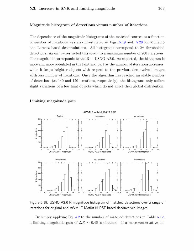
5.3. Increase in SNR and limiting magnitude 163
Magnitude histogram of detections versus number of iterations
The dependence of the magnitude histograms of the matched sources as a function
of number of iterations was also investigated in Figs. 5.19 and 5.20 for Moffat15
and Lorentz based deconvolutions. All histograms correspond to 2σ thresholded
detections. Again, we restricted this study to a maximum number of 200 iterations.
The magnitude corresponds to the R in USNO-A2.0. As expected, the histogram is
more and more populated in the faint end part as the number of iterations increases,
while it keeps brighter objects with respect to the previous deconvolved images
with less number of iterations. Once the algorithm has reached an stable number
of detections (at 140 and 120 iterations, respectively), the histograms only suffers
slight variations of a few faint objects which do not affect their global distribution.
Limiting magnitude gain
8 10 12 14 16 18 20USNO-A2.0 R magnitude
0
100
200
300
400
500
# de
tect
ions
Original
8 10 12 14 16 18 20USNO-A2.0 R magnitude
AWMLE with Moffat15 PSF10 iterations
8 10 12 14 16 18 20USNO-A2.0 R magnitude
60 iterations
8 10 12 14 16 18 20USNO-A2.0 R magnitude
0
100
200
300
400
500
# de
tect
ions
100 iterations
8 10 12 14 16 18 20USNO-A2.0 R magnitude
160 iterations
8 10 12 14 16 18 20USNO-A2.0 R magnitude
200 iterations
Figure 5.19: USNO-A2.0 R magnitude histogram of matched detections over a range of
iterations for original and AWMLE Moffat15 PSF based deconvolved images.
By simply applying Eq. 4.2 to the number of matched detections in Table 5.12,
a limiting magnitude gain of ∆R ∼ 0.46 is obtained. If a more conservative de-

164 Chapter 5. Results
8 10 12 14 16 18 20USNO-A2.0 R magnitude
0
100
200
300
400
500#
dete
ctio
nsOriginal
8 10 12 14 16 18 20USNO-A2.0 R magnitude
AWMLE with Lorentz PSF10 iterations
8 10 12 14 16 18 20USNO-A2.0 R magnitude
60 iterations
8 10 12 14 16 18 20USNO-A2.0 R magnitude
0
100
200
300
400
500
# de
tect
ions
100 iterations
8 10 12 14 16 18 20USNO-A2.0 R magnitude
160 iterations
8 10 12 14 16 18 20USNO-A2.0 R magnitude
200 iterations
Figure 5.20: USNO-A2.0 R magnitude histogram of matched detections over a range of
iterations for original and AWMLE Lorentz PSF based deconvolved images.
tection threshold of 3σ is considered for both original and deconvolved images, this
gain turns into a more favourable ∆R ∼ 0.59. Of course, although in this latter
the relative gain with respect to the original image is larger, the absolute limiting
magnitude in the 2σ case is deeper.
Note that gain estimate does not take into account the intrinsic magnitude dis-
tribution of the studied FOV, and could be somewhat biased. To check this, an
alternative estimate can be derived from the comparison of the original and decon-
volved images magnitude histograms with the histogram of USNO-A2.0. This is
illustrated in Fig. 5.21, where we overplot the magnitude histogram of the original
image with the one from a 140-iteration AWMLE Moffat15 deconvolution, and with
the complete histogram from USNO-A2.0. A similar magnitude gain can be derived.
Conclusions
We have applied AWMLE deconvolution to the NESS-T 02 frame. Its performance
was evaluated in terms of number of true and unmatched detections. The validation

5.3. Increase in SNR and limiting magnitude 165
8 10 12 14 16 18 20USNO-A2.0 R magnitude
0
250
500
750
1000
1250
1500
1750
# de
tect
ions
OriginalAWMLE 140-iterations Moffat15 PSFComplete USNO-A2.0
Figure 5.21: USNO-A2.0 R magnitude histograms of matched detections for the orig-
inal image and a 140-iteration AWMLE deconvolution with a Moffat15 PSF and a 2σ
detection threshold.
of true detections was carried out with USNO-A2.0 catalogue. The dependence
of those results on the chosen PSF model, the number of iterations and detection
threshold were also investigated.
AWMLE shows excellent performance in keeping the unmatched detections to
very low percentages (2-3%). It delivers limiting magnitude gains of ∆R ∼ 0.46 and
∆R ∼ 0.59 for 2σ and 3σ detections thresholds, respectively. This turns AWMLE
to be as a powerful technique for increasing the number of useful science objects
from the faint part of magnitude distribution.
A detailed analysis of the origin of those few unmatched objects was conducted.
The bulk of them were found to be caused by limited PSF knowledge and ringing
artifacts, which are accentuated by the severe original undersampling and inaccu-
rate background estimation. As a consequence of these two shortcomings, NESS-T
deconvolved images appear to be less converged than QUEST’s. This leads to a less
homogeneous detection process (this still depends on the chosen threshold), and a
smaller limiting magnitude gain (0.18 mag less) for the same detection threshold

166 Chapter 5. Results
as QUEST. However, it is noteworthy that a similar gain is obtained when a 3σ
detection threshold is considered.
The asymptotic convergence found for QUEST data in Sect. 5.3.1 was broken by
not having the original data properly calibrated (bias, darks and flats). This trans-
lated into a non-stability in the number of detections as a function of number of
iterations and a real dependence of number of detections with the considered thresh-
old. We emphasize that with these calibration frames, the performance of AWMLE
is likely to improve and recover the same level of convergence (and magnitude gain)
as QUEST data.
Finally, a comparative study between Moffat15 and Lorentz PSFs was made.
On one hand, the former delivered more matched detections. On the other hand,
the latter was shown to offer faster convergence (similar level of detections with 20
iterations less). This result is important if a systematic application of AWMLE to
NESS-T images is desired, since it saves execution time. In addition, thanks to
its better fit of the outer wings of the PSF, Lorentz based deconvolutions offered
significantly less false detections than Moffat15.
Possible extensions of this work
Being the Baker-Nunn Camera a wide field instrument, the increase of the limiting
magnitude shown in this section could be of interest for a large number of obser-
vational programs. In the particular case of NESS-T project, this could lead to an
important increase in its efficiency in terms of the number of detectable NEOs.
From the above mentioned constrains which introduce ∼ 2% of false detections,
at least the one refering to accurate background estimation could be easily solved
in near future when accurate flatfield calibration frames can be routinely obtained.
As a result, AWMLE convergence would be improved and false detections reduced
to an assumible percentage for a systematic usage in a dedicated NEOs detection
pipeline. For that purpose, with a 4K×4K CCD chip, execution time and RAM
usage of AWMLE are crucial issues for determining its feasibility. They were already
discussed in Table 2.1. As commented in QUEST case, an additional effort in the
algorithm optimization could improve the current performance up to shortening the
execution time by a 50%. In addition, by parallelizing the algorithm with as many
nodes as wavelet planes used in the decomposition of the original image (4 to 6)

5.4. Increase in resolution and object deblending 167
the scalability factor could be approximately proportional to the number of nodes
depending on the architecture implementation chosen. After all, execution time
could be safely reduced to a few seconds per iteration.
The presented results are totally general and are likely to be improved for data
sets with finer pixel scale. For example, a project like NOAO Deep Lens Survey
(DLS) (Becker et al. 2004; Wittman et al. 2002), would be an potential application of
AWMLE deconvolution. It is being operated on the 4 m Blanco and Mayall telescope
at the Cerro Tololo Inter-American Observatory (CTIO) and Kitt Peak National
Observatory (KPNO) with a 8K×8K CCD mosaic, yielding complete variability
census in the optical down to 24th magnitude. Given its fine scale of 0.′′26, the PSF
extraction could be largely improved in comparison to NESS-T case. As a result,
the performance of AWMLE algorithm would be improved to the level of QUEST
data in Sect. 5.3.1 or even better.
5.4 Increase in resolution and object deblending
This section will be devoted to assess the resolution gain obtained by image decon-
volution in QUEST and NESS-T data sets described in Chapt. 3.
5.4.1 QUEST: QSO candidates deblending for gravitational
lenses detection
In this section we will show how deblending capabilities of image deconvolution can
contribute to the detection of gravitational lenses among a list of QSOs8 candidates
culled from QUEST images. First, a brief overview of the current state of macrolens-
ing detection field will be given. Next, the results of the deconvolution for the two
data sets described in Table 3.9 will be presented. Finally, we will discuss the limits
and future extensions of this work.
A gravitational lens is one of the astrophysical observables predicted by General
Relativity. It appears when a very massive object (galaxy, massive black hole, etc.)
8We will use the terms QSO (quasi stellar object) and quasar as equivalent terms along this
section, although the concept quasar is often used only for radio sources.

168 Chapter 5. Results
deflects light coming from a very distant source, in most cases a quasar, and as a
result the observer can record a variety of phenomena such as Einstein Rings, the
amplification of the apparent intensity of the background source, or the splitting of
this source into two or more separated components.
It was early shown that crucial cosmological parameters (dark matter distribu-
tion, Hubble’s Constant through time delays between lens components and Ein-
stein’s Cosmological Constant) could be directly derived if a dense enough census of
lenses will be available in the future. Therefore, it was clear that intense and main-
tained observational effort should be dedicated in this topic. At a first stage, the
search was mainly conducted with VLBI observations among a selected sample of
already known quasars (8,609 (Veron-Cetty & Veron 1995)). This strategy yielded
to relatively scarse lenses discoveries (8 over a thousand of selected quasars by 1995)
since the first discovery of QSO 0957+561 by Walsh et al. (1979). In a second stage,
the new generation large QSO surveys, such as the SDSS (Loveday et al. 1998) and
the 2dF (Lewis et al. 1998), raised the number of catalogued quasars several up to
tens of thousands of entries (counting 48,921 in Veron-Cetty & Veron (2003)). This
shifted the lens search strategy towards a more exhaustive and unbiased one, based
on multi-band photometric variability and/or spectra classification criteria.
It is in this second framework which QUEST is currently working with a QSO
detection efficiency of ∼ 7% (Rengstorf et al. 2004a,b) by using a photometric vari-
ability criteria. As anticipated in Pag. 90, the strategy for lens searching is to
reobserve these QSOs candidates with larger telescopes equiped with high resolu-
tion CCDs. That is the case of follow-up campaigns conducted at WIYN telescope
with the MiniMosaic camera.
Our aim here is to see how deblending capabilities of image deconvolution could
help to resolve potentially lensed QSOs. As explained above, intensive follow-up ob-
servations at large telescopes are needed for lens detection, and if a more depurated
list of deblended candidates were available, that could be of crucial importance for
improving the confirmation efficiency.
Two different data sets were considered for the development of this work. They
consist of two different fields, labeled as Field 14 and Field 13, from which we
have QUEST (low resolution) and WIYN (high resolution) images, as described in
Table 3.9. The analysis procedure in both cases is the following:

5.4. Increase in resolution and object deblending 169
1. extract PSF from QUEST images as explained in Sect. 4.2,
2. perform deconvolution of QUEST images with the AWMLE algorithm de-
scribed in Sect. 2.3,
3. run SExtractor object detection (see Sect. 4.3) in all three images: WIYN
and original and deconvolved QUEST,
4. follow the methodology in Sect. 4.4.1 for validating detections between original
and deconvolved QUEST images, and the corresponding WIYN image,
5. apply the resolution assessment method described in Sect. 4.5.1 to those im-
age patches which comprise QSOs candidates culled by variability criteria and
compute image separation, magnitude and magnitude difference of newly re-
solved companions.
Field 14
QUEST and WIYN images considered in this case are q100899 F14 and w240700 F14,
as labeled in Table 3.9. Average seeing for QUEST data that night was around 2.′′4.
In Fig. 5.22 we illustrate the result after a 400-iteration deconvolution of the
QUEST image with the AWMLE algorithm. An hybrid Moffat25 PSF was used
since it was found to be the best fit to the original data, as explained in Sect. 5.1.2.
Attending the variability criteria explained above, up to 6 QSO candidates are in-
cluded in Field 14 for which we supply their corresponding USNO-B1.0 identificator
in Table 5.14. For each canditate panel in Fig. 5.22 we include three zoomed re-
gions: original QUEST, deconvolved QUEST and WIYN9. The background level
varies from image to image, mostly due to the proximity to bright stars (the most
notable case, C3).
9The zoom ratio for WIYN panels (1:6) is a bit smaller than the one for QUEST (1:7.3).

170
Chapte
r5.
Resu
lts
Cand
idat
e 4
QUEST QUEST deconvolved
QUEST QUEST deconvolved
WIYN
QUEST deconvolvedQUEST
WIYN
C5
C6
C4C4C4
C5 C5
C6C6
C3C3C3
C1C1
C2C2
Cand
idat
e 3
QUEST QUEST deconvolved
C1
QUEST QUEST deconvolved
WIYN
Cand
idat
e 2
Cand
idat
e 1
QUEST deconvolvedQUEST
WIYN
WIYNWIYN
Cand
idat
e 6
Cand
idat
e 5
C2
Figure 5.22: Application of image deconvolution to 6 QSO candidates in Field 14 field, described in Table 5.14. The original QUEST
frame is displayed in the centre. Each candidate panel includes original QUEST image, deconvolved QUEST image (400 iterations)
and high resolution WIYN image, respectively. The QSO candidates are labeled in each case. Ellipses indicate objects detected by
SExtractor. Those in green correspond to objects present in all three images, in blue those only resolved in WIYN and in red
those resolved both in WIYN and deconvolved QUEST images but not resolved in original QUEST image. This is the case of C5,
where deconvolution achieves to resolve the most distant component on the right of the sixtuple system.

5.4. Increase in resolution and object deblending 171
The detections labeled in green ellipses correspond to objects present in all three
images. Those in blue are objects only detected by WIYN. Finally, those in red are
detected both in WIYN and deconvolved QUEST images but not present in original
QUEST image.
Qualitatively, we can distinguish two causes which trigger the new detections in
the deconvolved QUEST image. On one hand, the increase in limiting magnitude:
this is the case of C2 and C3 red ellipses which are far from QSO candidate. On
the other hand, the increase of image resolution: this is the case of C5, where
deconvolution achieves to resolve the brightest companion of the sixtuple system.
Of course, both causes are not exclusive but they both simultaneously contribute
to new detections. Their relative importance depends mainly on the candidate-
companion separation and magnitude difference.
In Table 5.14 we summarize the results of what is shown in Fig. 5.22. The column
format for each candidate is: the second column corresponds to the id number in
USNO-B1.0 catalogue (Monet et al. 2003), 3rd to 5th columns indicate the resolving
status for all three kind of images, 6th to 9th columns are the parameters computed
from WIYN image for each component of the binary or multiple system. We decided
to split the resolving status into three separate categories: single, unresolved and
resolved. Below we discuss each one of these:
� Single source candidates
This is the case of candidates C1, C4 and C6, where even in high resolution
WIYN image they appear as unique components, without any near companion
which could be assumed to be a lens event.
Of course, in these cases image deconvolution cannot contribute to an improve-
ment of resolution, since the companion (if any) is much closer than the limit
which the AWMLE algorithm can reach with QUEST original sampling.
� Resolved candidate
this is the case of the D component of C5. This candidate is not resolved in
original QUEST image. On the contrary, the deconvolved QUEST image yields
a new component D at 4.′′0 from the candidate with a magnitude difference of
1.82, as determined from high resolution WIYN image. As seen in Fig. 5.23,
the presence of this companion was evident by eyeball already in the original
QUEST image. However, this detection proceduce is not practical given the

172 Chapter 5. Results
Table 5.14: Summary of image resolution improvement for the 6 QSO candidates (supplied by
Andrews (2000)) in Field 14 field after deconvolving QUEST image. Angular separation (ρ), magnitude
difference ∆m and magnitude of secondary component (m2) are derived from WIYN image.
Candidate Id USNO-B1.0 Id Resolving status(a) Companions parameters(b)
QUEST QUEST WIYN Id ρ ∆m m2
deconvolved (′′)
C1 0885-0528372 S S S - - - -
C2 0885-0528372 UR UR R B 3.2 1.15 15.17
UR UR R C 4.5 1.70 15.71
C3 0885-0527746 UR UR R B 1.9 0.61 13.52
C4 0884-0529657 S S S - - - -
C5 0884-0529982 UR UR R B 2.0 2.88 15.68
UR UR R C 2.7 2.73 15.53
UR R R D 4.0 1.82 14.62
UR UR R E 5.0 2.21 15.01
UR UR R F 5.7 3.41 16.21
C6 0883-0548350 S S S - - - -
(a) S: single, UR: unresolved, R: resolved.
(b) A given object in the vicinity of a candidate is considered to be a companion when its
separation is smaller than 7′′.
large extension of candidates list, which makes indispensable the use of an
automatic detection package as SExtractor, which in this case was not able
to deblend the companion from the candidate.
After a systematic search in NASA/IPAC Extragalactic Database (NED)10 and
SIMBAD11, we found no hit in either QSO catalogue or similar. SDSS database
was also queried, but coverage of this zone still remains to be done. Hence,
in absence of complementary information and spectroscopic confirmation, few
more can be said about the real nature of this candidate.
10The NASA/IPAC Extragalactic Database (NED) is operated by the Jet Propulsion Labora-
tory, California Institute of Technology, under contract with the National Aeronautics and Space
Administration.11SIMBAD database is operated at CDS, Strasbourg, France

5.4. Increase in resolution and object deblending 173
Candidate 2
Candidate 5
Candidate 3
C2 C2
C5C5
C2
C5
C3C3C3
B
B
D
EF
C
BC
Figure 5.23: A zoomed display of those panels in Fig. 5.22 which show unresolved (C2
and C3, top and middle) and resolved components (C5-D, bottom). The same ellipses,
colors and labeling criteria as Fig. 5.22 apply here.
� Unresolved candidates
These are the cases of B and C components of C2, B component of C3 and rest
of components (B,C,F and E) of C5, which are only resolved in high resolution
WIYN images.
All 7 components represent a good example of how different values for angular
separation and magnitude of the secondary can limit the image resolution of
an image. Below we describe them:
First, C3-B is unresolved despite of having a secondary one magnitude brighter
than C5-D, which is actually resolved. This is because its separation (1.′′9) is
cleary lower than in C5 case and below the seeing value at QUEST site for

174 Chapter 5. Results
that night (see Table 3.9). In addition, its closer magnitude difference does not
help the detection routine to deblend the companion. Although deconvolution
is not able to get the secondary detected, it is worth remarking that the object
ellipticity12 was found to be a bit larger (1.485 vs. 1.503) with respect to the
original image. That might be an indicator that C3 is a critically resolved
object.
Next, C2-B and C2-C are characteristic cases of moderate separation and
notably faint magnitude values. They are well above the seeing value (ρ = 3.′′2
and 4.′′5, respectively) and fainter (m2 = 0.6 and 1.1, respectively) than C5-D.
If one could compute the magnitudes of the companions in original QUEST
images, those would be below the corresponding limiting magnitude. Even
the ∆Vlim ∼ 0.6 gain supplied by deconvolution would not be sufficient in that
case.
Finally, an example of well separated but extremely faint components is rep-
resented by the C5-E and C5-F.
To sum up, C3-B could be considered as a critically unresolved case limited
mostly in terms of its close angular separation. In the other extreme, C5-E and C5-
F would be critically unresolved in terms of their faint limiting magnitude. C2-B
and C2-C can be considered as intermediate cases.
Field 13
QUEST and WIYN images considered in this case are q100899 F13 and w250700 F13,
as labeled in Table 3.9. The average seeing for QUEST data that night was around
2.′′3.
Note from Table 3.9, we have 5 QUEST frames of different nights covering the
same field Field 13. We chose only the one from Aug 10th 1999 for several reasons:
� in principle all 5 night frames could be coadded to obtain a deeper image,
comparable to WIYN limiting magnitude. However, we recall that what we
address in this section is the resolution gain introduced by the deconvolution
process. This strongly depends on the performance of the PSF extraction
12As computed by SExtractor.

5.4. Increase in resolution and object deblending 175
process. If we coadd frames with PSFs of different quality, the resulting image
is likely to have a complex PSF and a resolution worse than, at least, the best
of the input frames. To study the influence of the coadding process over the
PSF used for deconvolving is beyond the scope of this thesis.
Other coadding techniques in the superresolution context, such as drizzle al-
gorithm (Fruchter & Hook 2002), in combination with deconvolution, have led
promising results for undersampled images. However, this is equally outside
of the scope of this thesis.
� this was the night with best seeing. So it will allow us to estimate the maximum
absolute resolution attainable we can expect from QUEST data once they have
been deconvolved.
� this is the same night as previous q100899 F14 frame of Field 14. Therefore,
as seeing values recorded in chips B4 and C4 are pretty similar (see Table. 3.9),
we can assume that the results from Fields 14 and 13, in terms of resolution
gain, will be directly comparable.
Similarly to Field 14 example, an hybrid Moffat25 PSF was chosen for running
a AWMLE 300-iteration deconvolution. Field 13 is richer in QSO candidates, and
up to 38 of them have been studied this time.
A zoomed display of the three panels (original and deconvolved QUEST, and
WIYN) for each candidate can be seen in Figs. 5.24-5.29. The same labeling and
colors criteria as previous example were followed here. Note that in candidates
C7, C12, C23, C26, C28 and C29 a grey ellipse is shown, indicating detections of
deconvolution artifacts. The cause of this effect was already discussed in Sect. 5.3.1.
We briefly recall this is due to the fact that the mismatch in PSF extraction process
triggers false detections in the vicinity of bright stars when deconvolution is run to
a large number of iterations.
In Table 5.15 we summarize the results of what is shown in Figs. 5.24-5.29. The
column format is the same as Table. 5.14.

176 Chapter 5. Results
Table 5.15: Summary of image resolution improvement for the 38 QSO candidates (supplied by Snyder
(2001)) in Field 13 after deconvolving QUEST image. Angular separation (ρ), magnitude difference
∆m and magnitude of secondary component (m2) are derived from WIYN image.
Candidate Id USNO-B1.0 Id Resolving status1 Companions parameters2
QUEST QUEST WIYN Id ρ ∆m m2
deconvolved (′′)
C1 0891-0538903 UR UR R B 2.9 4.06 16.51
UR UR R C 3.4 4.05 16.50
C2 0891-0538916 UR UR R B 3.5 2.24 15.92
UR UR R C 4.1 1.94 15.62
UR R R D 4.8 0.28 13.97
UR R R E 5.8 1.76 15.44
C3 0891-0538962 R R R B 4.9 0.55 13.75
C4 0891-0538959 UR UR R B 5.2 2.75 16.01
UR R R C 6.2 2.31 15.57
UR UR R D 6.8 2.71 15.97
C5 0891-0538874 UR UR R B 4.0 5.83 15.80
C6 0891-0538922 UR R R B 4.9 2.99 14.94
UR UR R C 5.7 3.80 15.75
UR UR R D 5.7 4.22 16.18
C7 0891-0538934 UR UR R B 2.8 5.18 16.70
UR UR R C 4.5 4.60 16.12
UR UR R D 5.0 3.94 15.45
R R R E 6.0 2.46 13.98
C8 0891-0538827 UR UR R B 3.2 5.31 16.05
C9 0891-0538866 UR UR R B 5.5 3.72 16.47
R R R C 6.0 0.84 13.59
UR UR R D 6.2 3.27 16.04
C10 0891-0538869 UR R R B 5.7 2.55 15.32
UR UR R C 7.0 3.62 16.411 S: single, UR: unresolved, R: resolved.2 A given object in the vicinity of a candidate is considered to be a companion when its
separation is smaller than 7′′.Table continues on next page.

5.4. Increase in resolution and object deblending 177
Candidate Id USNO-B1.0 Id Resolving status1 Companions parameters2
QUEST QUEST WIYN Id ρ ∆m m2
deconvolved (′′)
C11 0891-0538897 UR UR R B 2.1 3.44 16.32
C12 0891-0538980 UR R R B 5.6 5.80 14.69
C13 0891-0538963 UR UR R B 1.8 0.80 14.21
UR UR R C 4.6 1.97 15.38
UR UR R D 6.3 2.60 16.01
C14 0891-0538977 UR UR R B 5.6 3.91 15.24
UR UR R C 5.8 4.42 15.75
UR R R D 6.3 2.78 14.11
C15 0892-0535528 UR UR R B 5.9 2.18 15.42
UR UR R C 6.0 3.13 16.36
C16 0892-0535541 UR UR R B 5.4 1.89 15.42
UR UR R C 6.2 2.84 16.36
C17 0891-0539018 UR UR R B 5.2 4.64 16.15
C18 0891-0539025 UR R R B 4.0 1.55 14.07
R R R C 6.0 1.43 13.95
C19 0891-0539033 R R R B 5.8 0.51 13.95
C20 0892-0535569 UR UR R B 1.2 2.09 15.00
C21 0892-0535592 S S S - - - -
C22 0891-0539078 UR UR R B 4.4 2.91 15.80
UR UR R C 4.4 3.55 16.45
C23 0891-0539083 UR UR R B 1.8 2.16 14.89
UR UR R C 5.7 2.88 15.61
C24 0891-0539059 R R R B 6.7 0.34 12.701 S: single, UR: unresolved, R: resolved.2 A given object in the vicinity of a candidate is considered to be a companion when its
separation is smaller than 7′′.Table continues on next page.

178 Chapter 5. Results
Candidate Id USNO-B1.0 Id Resolving status1 Companions parameters2
QUEST QUEST WIYN Id ρ ∆m m2
deconvolved (′′)
UR R R C 6.9 3.00 15.35
UR R R D 6.9 2.95 15.30
C25 0891-0539071 UR UR R B 2.2 2.35 15.75
C26 0891-0539050 UR UR R B 4.3 2.85 16.38
UR UR R C 6.6 2.98 16.51
UR UR R D 6.7 3.02 16.54
C27 0891-0539060 UR UR R B 1.3 2.82 15.65
UR UR R C 4.1 2.46 15.29
R R R D 4.9 1.39 14.22
UR UR R E 5.8 3.55 16.38
C28 0891-0539020 UR UR R B 6.5 5.16 14.08
C29 0891-0538983 R R R B 5.4 0.18 12.95
C30 0891-0538986 R R R B 5.4 -0.18 12.77
C31 0891-0539004 UR UR R B 3.3 3.23 16.06
UR UR R C 3.4 4.10 16.93
UR R R D 5.5 2.13 14.96
C32 0891-0539001 UR R R B 3.9 3.51 14.86
UR UR R C 5.2 6.02 17.37
R R R D 6.1 1.32 12.67
C33 0891-0539021 UR UR R B 4.7 4.33 15.99
UR UR R C 6.2 4.13 15.79
C34 0891-0538970 UR UR R B 3.7 5.26 17.15
C35 0891-0538985 UR UR R B 2.5 4.55 16.18
UR R R C 4.7 2.59 14.22
UR UR R D 6.6 2.81 14.43
1 S: single, UR: unresolved, R: resolved.2 A given object in the vicinity of a candidate is considered to be a companion when its
separation is smaller than 7′′.Table continues on next page.

5.4. Increase in resolution and object deblending 179
Candidate Id USNO-B1.0 Id Resolving status1 Companions parameters2
QUEST QUEST WIYN Id ρ ∆m m2
deconvolved (′′)
C36 0891-0538981 UR UR R B 3.8 3.18 16.34
UR UR R C 5.2 2.37 15.53
C37 0891-0538999 UR UR R B 2.5 4.23 16.68
UR UR R C 5.3 4.77 17.22
UR R R D 5.9 1.50 13.95
UR UR R E 6.2 3.47 15.93
C38 0891-0538980 UR R R B 5.4 1.82 13.73
UR UR R C 5.6 3.50 15.41
1 S: single, UR: unresolved, R: resolved.2 A given object in the vicinity of a candidate is considered to be a companion when its
separation is smaller than 7′′.
As in the Field 14 case, below we discuss the three separate categories: single,
unresolved and resolved:
� Single source candidates
This is the case of candidate C21, where even in high resolution WIYN image
it appears as a single component, without any companion within 7′′ which
could be assumed to be a lens event.
Of course, in these cases image deconvolution cannot contribute to an improve-
ment of resolution, since the companion (if any) is much closer than the limit
that AWMLE can reach with QUEST original sampling.
� Resolved candidates
Among the 38 candidates in Table 5.15, 20 of them show a total of 25 resolved
components. 10 of these components were already detected in the original
QUEST images. The 15 remaining were resolved only in the deconvolved
QUEST and WIYN images. The separation of these newly detected compan-
ions ranges from 3.′′9 to 6.′′9.
As seen in Figs. 5.24-5.29, most of the companions triggered by AWMLE
could be guessed by visual inspection already in the original QUEST image.

180 Chapter 5. Results
However, SExtractor, even with optimized input parameters, was not able to
deblend them from the primary.
As in Field 14, a systematic search in NED and SIMBAD databases was performed
with no positive hits which could reveal additional information about the QSO
nature of these multiple candidates.
� Unresolved candidates
There are 17 candidates and 54 components in Table 5.15 which could only
be resolved by high resolution WIYN images. They cover a wide range of sep-
arations, magnitude of secondaries and difference of magnitudes. We discuss
some representative cases for each parameter:
C13-B is unresolved because of its close separation to primary (1.′′9) and de-
spite of having a secondary a magnitude brighter than other resolved fainter
components. Thus, this is a clear example of a critically unresolved candidate
mostly because of its close angular separation, which is below the seeing value
at QUEST site for that night (2.′′0).
C1-C and C14-B are characteristic cases of moderate separation and notably
faint magnitude values. They are well above the seeing value (ρ = 3.′′4 and
5.′′6, respectively) but significantly fainter than other resolved components. In
other words, those candidates are critically unresolved because of their faint
limiting magnitude.
Quantitative assessment of resolution gain
In Field 14 example we qualitatively anticipated that both the increase in limiting
magnitude and the gain image resolution contribute to new components detected
in deconvolved QUEST images. We also pointed out that each one of these causes
become dominant over the other depending on the particular combination of image
separation, secondary magnitude and magnitude difference of every component.
In order to establish a quantitative study of resolution gain, the methodology
described in Sect. 4.5.2 was followed. We grouped all the QSOs candidates from
Fields 14 and 13 examples (44 in total), and plotted the separation (ρ) of all the
resolved components as a function of their magnitude (m2) in Fig. 5.30, and the
magnitude difference (∆m) as a function of (ρ) in Fig. 5.31. As previous figures,

5.4. Increase in resolution and object deblending 181
C3
Candidate 1 − USNO−B1.0 0891−0538903
Candidate 2 − USNO−B1.0 0891−0538916
Candidate 3 − USNO−B1.0 0891−0538962
Candidate 4 − USNO−B1.0 0891−0538959
Candidate 5 − USNO−B1.0 0891−0538874
C5 C5 C5
C4C4C4
C3 C3
C2C2C2
C1 C1 C1
B
C
B
C
DE
B
B
D
C
BC
Figure 5.24: QUEST, original and deconvolved, and WIYN panels of QSO candidates
included in Table 5.15. Their resolved components are labeled accordingly to the same
table. Green ellipses for objects present in all three images, red for those detected both
in WIYN and deconvolved QUEST, but not in original QUEST image, and blue for those
only detected by WIYN.

182 Chapter 5. Results
Candidate 6 − USNO−B1.0 0891−0538922
Candidate 7 − USNO−B1.0 0891−0538934
Candidate 8 − USNO−B1.0 0891−0538827
Candidate 9 − USNO−B1.0 0891−0538866
Candidate 10 − USNO−B1.0 0891−0538869
C10
C6 C6 C6
C8C8C8
C10C10
C9 C9 C9
C7C7
C7
B
C
D
B
C
D
E
B
B
D
C
BC
Figure 5.25: QUEST, original and deconvolved, and WIYN panels of QSO candidates
included in Table 5.15. Their resolved components are labeled accordingly to the same
table. Green ellipses for objects present in all three images, red for those detected both
in WIYN and deconvolved QUEST, but not in original QUEST image, and blue for those
only detected by WIYN.

5.4. Increase in resolution and object deblending 183
Candidate 11 − USNO−B1.0 0891−0538897
Candidate 12 − USNO−B1.0 0891−0538980
Candidate 13 − USNO−B1.0 0891−0538963
Candidate 14 − USNO−B1.0 0891−0538977
C17
C15
C16C16
C15
C17C17
C16
C15
C14C14C14
C13C13C13
C12C12
C11C11
Candidates 15,16 and 17 − USNO−B1.0 0892−0535528, 0892−0535541 and 0891−0539018
C11
C12
B
B
B
C
D
BC
D
C15−B
C15−C
C16−C
C16−BC17−B
Figure 5.26: QUEST, original and deconvolved, and WIYN panels of QSO candidates
included in Table 5.15. Their resolved components are labeled accordingly to the same
table. Green ellipses for objects present in all three images, red for those detected both
in WIYN and deconvolved QUEST, but not in original QUEST image, and blue for those
only detected by WIYN.

184 Chapter 5. Results
Candidate 20 − USNO−B1.0 0892−0535569
Candidate 21 − USNO−B1.0 0892−0535592
Candidate 22 − USNO−B1.0 0891−0539078
C18
C19
C18
C23
C19C19
C23
C18
C23
Candidate 23 − USNO−B1.0 0891−0539083
C22C22C22
C21 C21C21
Candidates 18 and 19 − USNO−B1.0 0891−0539025 and 0891−0539033
C20C20C20
B
C18−BC18−C C19−B
B
C
CB
Figure 5.27: QUEST, original and deconvolved, and WIYN panels of QSO candidates
included in Table 5.15. Their resolved components are labeled accordingly to the same
table. Green ellipses for objects present in all three images, red for those detected both
in WIYN and deconvolved QUEST, but not in original QUEST image, and blue for those
only detected by WIYN.

5.4. Increase in resolution and object deblending 185
Candidate 28 − USNO−B1.0 0891−0539020
Candidates 24 and 25 − USNO−B1.0 0891−0539059 and 0891−0539071
Candidates 26 and 27 − USNO−B1.0 0891−0539050 and 0891−0539060
Candidates 29, 30 and 31 − USNO−B1.0 0891−0538983, 0891−0538986 and 0891−0539004
Candidates 32 and 33 − USNO−B1.0 0891−0539001 and 0891−0539021
C24
C25
C24
C25
C24
C25
C26C26
C27C27C27
C26
C28C28C28
C30
C29
C31C31
C30
C29
C31
C30
C29
C33
C32
C33
C32
C33
C32
B
C24−D
C24−CC24−B
C25−B
C26−C
C26−D
C26−B
C27−C
C27−D
C27−B
C27−E
C29−BC30−B
C31−C C31−B
C31−D
C33−B
C33−C
C32−BC32−C
Figure 5.28: QUEST, original and deconvolved, and WIYN panels of QSO candidates
included in Table 5.15. Their resolved components are labeled accordingly to the same
table. Green ellipses for objects present in all three images, red for those detected both
in WIYN and deconvolved QUEST, but not in original QUEST image, and blue for those
only detected by WIYN.

186 Chapter 5. Results
Candidates 34 and 35 − USNO−B1.0 0891−0538970 and 0891−0538985
Candidates 36, 37 and 38 − USNO−B1.0 0891−0538981, 0891−0538999 and 0891−0538980
C34
C35 C35
C34 C34
C35
C36C38
C37
C36C38
C37
C36C38
C37
C35−DC35−B
C35−C
C34−B
C37−E
C36−C
C37−DC37−B
C36−BC38−C
C38−B
C37−C
Figure 5.29: QUEST, original and deconvolved, and WIYN panels of QSO candidates
included in Table 5.15. Their resolved components are labeled accordingly to the same
table. Green ellipses for objects present in all three images, red for those detected both
in WIYN and deconvolved QUEST, but not in original QUEST image, and blue for those
only detected by WIYN.
green circles indicate those resolved in all three images (original and deconvolved
QUEST and WIYN), red those resolved in deconvolved QUEST images and WIYN,
and blue those only resolved by WIYN.
In Fig. 5.30, the three categories (colors) of resolving status are disposed in
differentiated regions of the (ρ,m2) space.
As expected, blue circles populate the faint and high resolution ends of the
plot. The component C28-B (m2 = 14.08, ρ = 6.′′5) and the component C35-D
(m2 = 14.43, ρ = 6.′′6), constitute the exception to this rule. Despite of being
brighter than other resolved components at less favourable separations (C35-C, for
example), they could not be resolved in deconvolved image because of their proximity
to other stars in the field (see Figs. 5.28 and 5.29).
The bright and low resolution end is populated, first by red and finally by green
circles. The component C32-B, point (m2 = 14.86, ρ = 3.′′9), corresponds to the
closest companion resolved in deconvolved QUEST images, while the component

5.4. Increase in resolution and object deblending 187
12 13 14 15 16 17 18m2 of resolved component
0
2
4
6
8
ρ (a
rcse
c)
Figure 5.30: The separation of the resolved components in Fields 14 and 13 is plotted
as a function of their instrumental magnitude measured in WIYN. Green diamonds in-
dicate objects present in all three images, red pluses those detected both in WIYN and
deconvolved QUEST, but not in original QUEST image, and blue circles for those only
detected by WIYN.
0 2 4 6 8ρ (arcsec)
0
2
4
6
∆m
Figure 5.31: The magnitude difference of the resolved components in Fields 14 and 13
is plotted as a function of their separations. Green diamonds indicate objects present in
all three images, red pluses those detected both in WIYN and deconvolved QUEST, but
not in original QUEST image, and blue circles for those only detected by WIYN.

188 Chapter 5. Results
C27-D, point (m2 = 14.22, ρ = 4.′′9), turns to be the faintest and closest to be re-
solved in original QUEST images. From that we can derive that image deconvolution
increases the image resolution in about 1′′. This improvement could be even larger
with better knowledge of original PSF. Of course, this is only an estimate since the
statistics of our candidates sample is not complete in terms of (ρ,m2) space density.
As regard as Fig. 5.31, we note that newly resolved components by AWMLE
deconvolution are distributed along a wider range of ∆m. It is remarkable that C32-
B, resolved at ρ = 3.′′9 in the deconvolved image, is 3.51 fainter than its companion.
This is a magnitude difference 1.39 mag fainter than C27-D, resolved at ρ = 4.′′9 in
the original image.
We put this result into the context of current state of macrolensing field by mak-
ing the following remarks. As a result of the recent injection of new QSOs from
photometric and spectroscopic surveys, the number of discovered lenses has been
constantly increasing and some descriptors as separation distribution can already
be considered statistically significant. Fig. 5.32 illustrates the histogram of angular
separation between farthest components of known gravitational lenses up to now.
This is a 82 object sample catalogued by Kochanek et al. (2005), which spans from
widest to closest separation values. It can be seen that the bulk of lenses compan-
ions are comprised within 2′′ of separation and they are very rare beyond 4′′. It
is noteworthy that the limiting resolution of deconvolved QUEST images (3.′′9) is
within this cutoff value of 4.′′0 in Fig. 5.32. This enables deconvolved QUEST data to
directly resolve lenses, at least in a small percentage of the separation distribution,
and establish a significant difference with respect to the original images, where the
resolution limit of 4.′′9 vanishes the probability of direct resolving.
Of course, lenses will always need to be confirmed with high resolution imagery
(WIYN, HST, etc.), but to have a QUEST limiting resolution around the same value
where the lens population begins to increase could be useful for obtaining a list of
resolved QSO candidates more likely to be really lensed.
Conclusions
At this point, a number of conclusions can be drawn:
� AWMLE deconvolution increases the resolution of the QUEST images by 1′′,

5.4. Increase in resolution and object deblending 189
0 2 4 6 8 10 12 14 16 18 20Angular separation (arcsec)
0
5
10
15
20
Num
ber o
f kno
wn
lens
es
Resolution limit of original QUEST data
Resolution limit of QUEST deconvolved data
Figure 5.32: Histogram of angular separation for known gravitational lenses (Kochanek
et al. 2005). Deconvolution shifts the limiting resolution of QUEST data to 3.′′9, just
below the cutoff value at 4.′′0.
from 4.′′9 to 3.′′9. For the sake of comparison, this improvement (∼ 26%)
turns to be about twice the smearing introduced by drift scanning, as seen in
Table 3.11 and explained in Pag. 94.
� The limiting resolution after deconvolution of QUEST images is 3.′′9, which is
within the cutoff value of the separation distribution of the 82 gravitational
lenses currently known (Kochanek et al. 2005). This enables QUEST data for
potentially resolving lensed QSOs directly from deconvolved data. Of course,
high resolution images continue to be necessary for confirming lens geometry.
� The limiting magnitude gain of 0.6 mag derived in Sect. 5.3.1 is parallely
confirmed on average in Fig. 5.30. Actually, there are 5 red points which
exceed this gain value. However, we note that m2 is only an instrumental
magnitude, which has not been calibrated to be comparable to the study made
in Sect. 5.3.1 with catalogued magnitude.

190 Chapter 5. Results
Possible extensions of this work
We have shown that AWMLE deconvolution can deliver a resolution gain of 1′′ for
moderately undersampled data like QUEST (FWHM∼ 2.′′3).
The followed methodology for applying image deconvolution to QSO candidates
resolution is totally general, and other ongoing multiband wide field surveys in the
seek of new quasars could benefit from the achieved increase in resolution. For
example, projects like Palomar-QUEST (Djorgovski et al. 2004a,b) (with pixel scale
of 0.′′88) and SDSS (with median PSF FWHM of 3.2 pixels), would be suitable targets
for gaining additional resolution through image deconvolution. As resolution gain
strongly depends on the adequate modelling and characterization of the PSF, and
this depends basically on sampling, we anticipate that the former resolution gain is
expected to be better than 1 pixel for these two better sampled surveys.
SDSS Data Release 3 (6TB of images) (Abazajian et al. 2005) and its correspond-
ing Quasar catalogue (∼ 46, 420 entries) (Schneider et al. 2005) have been recently
offered to the community. From the combination of these two products, plus follow-
up high resolution observations, up to 12 lensed quasars of 260 candidates have
been confirmed (Pindor 2004). This applied candidate selection algorithm is able to
resolve components down to separations of ρ = 0.′′6 with ∆m = 0 and ρ = 1.′′2 with
∆m ∼ 3. Taking into account the resolution gain of 1 pixel deduced from Figs. 5.30
and 5.31, components separations up to 0.′′5 with ∆m = 0 and 0.′′75 with ∆m ∼ 3.5
could be attainable for SDSS data after AWMLE deconvolution. This gain could be
even better given the finer PSF sampling of SDSS with respect to QUEST. There-
fore, we emphasize the convenience of applying AWMLE deconvolution to this data
set, in order to consider this improved geometry separation as an additional criteria
for lensed quasar candidate selection.
As both surveys, Palomar-QUEST and SDSS, are operated under drift scanning
and TDI schemes, respectively, their data throughput rate is extremely high (several
Tbs/night). One could object that the application of image deconvolution to this
kind of data is not feasible by computational constrains. However, note that this
application does not aim to deconvolve the whole image archive. On the contrary,
we recall the objective is to resolve QSOs candidates from a list previously culled by
variability criteria. Therefore, the computer resources can be focused to deconvolve
only small patches (256x256 pixels) containing those objects. As shown in Table 2.1,

5.4. Increase in resolution and object deblending 191
the performance of AWMLE algorithm with images of this size is of about 42 itera-
tions per minute (a typical 300 iteration run in just 7.1 minutes) without aceleration
parameter in AWMLE. Therefore, although the number of candidates is relatively
large (several tens of thousands for SDSS Quasar catalogue Data Release 3), the
feasibility of the deconvolution is fully assured.
Other deconvolution algorithms with the same purpose of resolution increase
exist in the literature. Just to mention two examples: Eigenbrod et al. (2005a,b,c)
have recently applied the 1-D version of their MCS deconvolution algorithm (Magain
et al. 1998) to VLT/FORS spectra of lensed quasars for determining H0 from the
time delay method. Also, ’HiRes’ software (Velusamy et al. 2004) was being applied
for deconvolving SPITZER images, delivering an increase in the angular resolution
by a factor of two. This major achievement, shows that image deconvolution can
be even more effective in space-based data, where PSF modelling is usually more
accurate than in ground-based data.
5.4.2 NESS-T
We here repeat the analysis of resolution gain for NESS-T images. The aim of this
study is to estimate how the deblending capabilities of image deconvolution can
help to improve NESS-T original resolution. We emphasize that, in the particular
case of this data where pixel scale is so coarse (3.′′9 per pixel), whatever increase in
resolution is of importance for extending the range of scientific targets, in this case
NEOs.
The considered frame was NESS-T 2, which was described in Sect. 3.2.3. The
election of this frame is justified because it is one of the best in Table 3.13 in terms
of resolution, as can be deduced from FWHM histograms in Fig. 3.21. Therefore,
the resulting derived resolution gain (which is a relative quantity) will also give us
an upper estimate of the best absolute resolution attainable, at least for the night
we are considering.
The PSF extraction was performed in a very similar fashion to the limiting
magnitude study. See Sect. 5.1.3 for more details.
As regard as image deconvolution, we only used AWMLE given the clear in-
capacity of Richardson-Lucy algorithm for keeping false detections to a reasonable

192 Chapter 5. Results
level, as was shown in Sect. 5.3.1. The rest of parameters for the deconvolution runs
were identical to the ones in Table 5.11.
As SExtractor detections, a different set of parameters was used. In particular,
the minimum area for a positive detection was set to 3 pixels. In addition, the
convolution kernels widths used for enhancing the detection maps were set to the
actual values of FWHM for both original and deconvolved images. Finally, the same
process for matching and validating these detections with USNO-A2.0 catalogue
described in Pag. 153 was followed.
Both the qualitative and quantitative approaches in Sect. 4.5.1 and 4.5.2 for
assessing the resolution gain were considered in this section. This constrasts to the
only usage of the qualitative method in Sect.5.4.1, where the individual resolving
status for a set of 44 selected QSO candidates was calculated.
Below we present the results from the application of this algorithm.
Qualitative assessment of resolution gain
We first apply the methodology anticipated in Sect. 4.5.1 to the object pairs with
minimum separation in original and deconvolved images. For the latter, the two
combinations of PSF and number of iterations which offered closest resolved objects
were Moffat15 and Lorentz PSFs with 140 and 120 iterations, respectively. These
three objects, D0, D1 and D2 are illustrated in Fig. 5.33. For each panel, the original
image in the left and its corresponding deconvolved version in the right are shown.
Their separation values are stored in Table 5.16. In addition, the corresponding
USNO-B1.0 object for each component is included with its catalogued magnitude.
Below we separately discuss these three closest resolved objects:
� D0 is the closest pair resolved in the original image. Of course, this object
is also deblended in all the deconvolved images (not only in the two we are
considering). Moffat15 140-iteration deconvolution is displayed in the right
side of top panel.
� D1 is the closest pair resolved in Moffat15 140-iteration deconvolved image,
and, actually, in all the deconvolutions along the considered iterations range
(10–600) and PSFs. However, because of its faint magnitude it is not detected

5.4. Increase in resolution and object deblending 193
Figure 5.33: D0, D1 and D2 are the three closest objects resolved in NESS-T original,
140-iteration Moffat15 and 120-iteration Lorentz deconvolved images, respectively. Their
components separations are 3.69 pixels (14.′′4), 2.68 pixels (10.′′4) and 2.95 pixels (11.′′5),
leading to resolution gains of (4.′′0) in Moffatt15 case and (2.′′9) in the Lorentz case. Left
side panels are NESS-T original images: object detection circled in red. Both D1 and
D2 are unresolved. Right side panels are AWMLE deconvolved images: 140-iteration
Moffat15 for D0 and D1 and 120-iteration Lorentz for D2. The objects already detected
on the left are circled in red, and those newly detected are in green. It is noteworthy the
different SNR domain in which D1 and D2 are resolved. On one hand, D1 is an example
of a couple recovery with very faint components. On the other hand, D2 represents
the opposite situation of two bright components of similar magnitude. Note that D1-A,
although being detected as single source in deconvolved image, it is really composed by
the blending of three USNO-B1.0 faint sources (see Table 5.16).

194 Chapter 5. Results
Table 5.16: Three closest detections in original, 140-iteration Moffat15 and 120-iteration
Lorentz deconvolved images. Angular separation is between components A and B in
Fig. 5.33. The two columns on the right are USNO-B1.0 stars approximately coincidents
with D0, D1 and D2 components. Note the special case of the D1-A detection, which
includes three very close catalogue entries.
NESS-T resolved detections USNO-B1.0 objects
Id Component Id ρ(′′) Id R1 mag
D0 A 14.′′4 1293-0285550 14.29
B 1293-0285558 14.40
D1 A 10.′′4 1296-0294046 19.19
A 1296-0294054 17.96
A 1296-0294058 19.06
B 1296-0294064 19.08
D2 A 11.′′5 1292-0282993 14.56
B 1292-0282995 14.22
in the original image. With respect to D0, D1 represents a resolution gain of
1.01 pixels (4.′′0).
As was pointed out in Sect. 5.4.1, both the increase in limiting magnitude
and the resolution gain contribute to newly detected close components. D1
contitutes a paradigmatic example of this synergy: without the SNR increase,
it would have not been detected and, consequently, resolved.
Although D1 is resolved as to be double in NESS-T deconvolved image, note
that D1-A component is really composed by three USNO stars: USNO-B1.0 1296-
0294046, USNO-B1.0 1296-0294054 and USNO-B1.0 1296-0294058. As seen in
Table 5.16, the main part of the flux is supplied by USNO-B1.0 1296-0294054,
which is more than a magnitude brigther than the other two companions. De-
spite USNO-B1.0 1296-0294046 and USNO-B1.0 1296-0294058 being as faint
as D1-B component, they could not be resolved because their even closer sep-
arations.
� D2 is the closest pair resolved in Lorentz 120-iteration deconvolution. With
respect to D0, D2 represents a resolution gain of 0.74 pixels (2.′′9). Note in
lower left panel of Fig. 5.33 that D2, in contrast to D1, is actually detected in
the original image, although as a single object. Only in the deconvolved image

5.4. Increase in resolution and object deblending 195
the resolution is high enough to deblend the two components, A and B.
With respect to D1, D2 represents the opposite situation as magnitude of
their components. Both are bright objects well above the limiting magnitude
of NESS-T original image. Therefore, in this case the resolving of D2 can be
exclusively attibuted to the deblending capabilities of AWMLE deconvolution.
Note that the aim of this subsection was to provide a first estimate of the resolu-
tion gain introduced by AWMLE deconvolution. A more complete and quantitative
study in the style of Sect. 4.5.1 is detailed below.
Quantitative assessment of resolution gain
A direct indicator of the resolution gain between original and deconvolved images is
to compare the corresponding histograms of separations for closest resolved objects.
These can be seen in Fig. 5.34, for 140-iteration Moffat15 and 120-iteration Lorentz
PSF based deconvolutions, respectively. For the sake of comparison, the histogram
from original image was superposed in both cases.
Due to the increase in SNR introduced by AWMLE deconvolution described in
Sect. 5.3.1, the histograms of deconvolved images show larger number of events. Note
that most part of these new objects are incorporated in short end of the histogram
(ρ < 10 pixels).
We define the limiting resolution of a given image ρlim as the shortest separation
detected in it. This minimum separation corresponds to D0, D1 and D2 objects
displayed in Fig. 5.33 and discussed in previous subsection. ρlim has been computed
and labeled for every histogram in Fig. 5.34. ρlim was found to be 3.69 pixels (14.′′4),
2.68 pixels (10.′′4) and 2.95 pixels (11.′′5) in the original, AWMLE 140-iteration Mof-
fat15 and AWMLE 120-iteration Lorentz deconvolved images, respectively. This
translates into a resolution gain of (3.′′9) in Moffatt15 case, and (2.′′9) in the Lorentz
case. It is noteworthy that, at least for the former, the gain is well larger than the
seeing that night.
Four comments are worth emphasizing from Fig. 5.33:
1. the two considered deconvolution runs were the ones showing the maximum

196 Chapter 5. Results
resolution gain over all the rest of performed deconvolutions (from 10 to 200
iterations).
2. the resolution gains from these images differ slightly, only a ∼ 9%.
3. the derived resolution gains were accomplished at the same number of itera-
tions which a maximum of limiting magnitude gain was found in Sect. 5.3.2
(140-it. and 120-it.).
4. at least for the 140-it. Moffat15 deconvolution, the resolution gain in terms
of pixel units is nearly identical to the one obtained with QUEST data in
Sect. 5.4.1. This fact indicates that, at the level of the constrains (sampling
and limited PSF modeling) appearing in NESS-T and QUEST data, AWMLE
deconvolution achieves similar resolution performance in a similar number of
iterations. In other words, for two independent data sets (QUEST and NESS-
T), AWMLE appears to inject the same bulk of resolution after an intermediate
range of iterations (200–400) is run.
Next we consider the relation between the object separation of all the resolved
components as a function of their magnitude difference (∆R), as illustrated in
Fig. 5.35. In general, the objects distribution is more concentrated around ∆R ∼ 0.
In detail, they are cone-like distributed with its vertex in abscisa ρlim. This is due
to the fact that the fainter is a component with respect to its companion, the harder
is to deblend them as we approach one to each other. SExtractor tries to overcome
this by using a deblending method based on multi-thresholding scheme, which is
tuned by DEBLEND MINCON and DETECT MINAREA parameters. However, its perfor-
mance is limited, and normally excludes to separate objects with a difference in
magnitude greater than ∼ 8 mag (Bertin & Arnouts 1996).
From the inspection of Fig. 5.35, two differences can be appreciated between
the distribution of objects from original and deconvolved images. On one hand,
the vertex of the distribution is shifted towards closer separations in the case of
deconvolved image. This is equivalent to the limiting resolution gain (ρlim) derived
above. On the other hand, the opening angle of the cone-like distribution is larger for
deconvolved image. As a result, fainter companions can be resolved at separations
which remained inaccessible in the original image.
Note also that the larger separation end lacks objects from deconvolved image
(red pluses). This is a natural consequence of the fact that those objects with far

5.4. Increase in resolution and object deblending 197
0 5 10 15 20 25 30ρ (pixels)
0
25
50
75
100
125
Num
ber o
f res
olve
d ob
ject
sOriginalAWMLE 140 iterations Moffat15 PSF
0 5 10 15 20 25 30ρ (pixels)
0
25
50
75
100
125
Num
ber o
f res
olve
d ob
ject
s
OriginalAWMLE 120 iterations Lorentz PSF
deconvolved image
NESS−T original image
Limiting resolution of NESS−T
Limiting resolution of
deconvolved imageLimiting resolution of NESS−T
NESS−T original imageLimiting resolution of
Figure 5.34: Histogram of separation of closest resolved objects up to 30′′. Limiting
resolution is 3.69 pixels (14.′′4), 2.68 pixels (10.′′4) and 2.95 pixels (11.′′5) for the origi-
nal, AWMLE 140-iteration Moffat15 (top) and AWMLE 120-iteration Lorentz (bottom)
deconvolved images, respectively.

198 Chapter 5. Results
0 5 10 15 20 25 30ρ (pixels)
-10
-5
0
5
10
∆ROriginalAWMLE 140-it. Moffat15 PSF
Figure 5.35: Magnitude difference of closest resolved objects versus their separation,
for original (circles in black) and AWMLE 140-iteration Moffat15 deconvolved (pluses in
red) images, respectively.
companions in the original image have been repaired to new closer companions after
AWMLE deconvolution. As a result, the plot of red pluses is more compressed
towards lower separations.
The equivalent of Fig. 5.35 for 120-iteration Lorentz PSF deconvolution was not
included because the results are totally equivalent.
Conclusions
A qualitative and quantitative study of the resolution gain introduced by AWMLE
deconvolution in NESS-T images was carried out. A number of conclusions can be
drawn:
1. AWMLE deconvolution increases the resolution of the NESS-T data by 3.′′9.
For the sake of comparison, this improvement is well larger than the seeing
for that night (. 3′′) and about 14 times the smearing introduced by pixel
response function, as seen in Table 3.14 and explained in Pag. 102.

5.4. Increase in resolution and object deblending 199
2. In terms of pixel units, this resolution gain corresponds to ∼ 1.0 pixels. This
is nearly the same gain obtained for QUEST data in Sect. 5.4.1. This is re-
markable, and it addresses an interesting point: although the pixel scales of
both data sets differ significantly (1′′ to 3.′′9), their sampling (FWHM) is nearly
identical. Consequently, we can conclude that the resolution gain mainly de-
pends on sampling, and is only sightly modulated by other constrains (drift
scanning systematics, correct flatfield calibration and limited PSF modeling).
3. The derived resolution gain shows slight dependence over the PSF chosen in
the deconvolution process. At maximum, differences between Moffat15 and
Lorentz PSFs of only ∼ 9% are observed.
4. The maximum resolution gain is accomplished around 140 and 120 iterations,
for Moffat15 and Lorentz PSF based deconvolutions, respectively. These are
the same iteration numbers where limiting magnitude gain was also maximized
in Sect. 5.3.2. This coincidence is indicating that optimal convergences for
magnitude and resolution studies are simultaneously reached.
5. As deduced from Fig. 5.35, deconvolution enables the detection of companions
comprised at a range of separation and magnitude difference which was totally
forbbiden in the original image.
Possible extensions of this work
We have shown how AWMLE deconvolution can improve significantly the resolution
of a wide field facility with coarse pixel scale as NESS-T.
Of course, as pointed out in Sect. 5.3.2, AWMLE deconvolution could be in-
serted in the reduction pipeline of NESS-T data. Once the flatfield calibration and
computation time constrains are solved, this is an option to be seriously considered
for increasing the detection efficiency of NEOs survey.
Apart from NESS-T, there are a number of similar observational projects which
could benefit of this resolution gain. Just as an example, we briefly justify the
potential of applying deconvolution for resolving binary asteroids:
Up to the present, the discovery of binary asteroids, specially NEOs, has been
conducted by time-resolved photometric observations (lightcurves) (Pravec et al.

200 Chapter 5. Results
2004, 2005). A period analysis by Fourier series (Harris et al. 1989; Pravec et al.
2000) can provide indirect evidence of binarity (Pravec et al. 2002), which is poste-
riorly confirmed by space based imaging (HST) or radar observations (Busch et al.
2005). Apart from being indirect, the detection by lightcurves is time consuming.
As a result, this turns to be a relatively low efficiency technique, and the binarity
of only a very small percentage of known asteroids has been studied.
Only recent advances in adaptive optics (AO) imagers as VLT/NACO have en-
abled the direct detection of binary asteroids. For example, the case of the triple
main-belt asteroid 87 Sylvia (Marchis et al. 2005) led to components separation up
to 0.′′17 and 0.′′84, with ∆m < 3.8 and ∆m < 4.2. Of course these AO systems
are very competitive facilities and cannot be dedicated to intensive search of binary
asteroids.
However, the application of AWMLE deconvolution to medium resolution all-
sky surveys could be decisive in the aim of directly resolving binary asteroids. For
example, projects like SDSS (already active), PAN-STARR13 and LSST14 (Claver
et al. 2004) have well sampled FWHMs in the 0.′′8–0.′′5 range. In these conditions,
better than those exhibited by QUEST and NESS-T, AWMLE deconvolution is ex-
pected to accomplish even better resolution gain (1–1.5 pixel). In that case, asteroid
components separated within 0.′′4–0.′′25 could be resolvable, and this would open the
possibility of massively detecting binary asteroids. As the existence of most of the
imaged asteroids would be a priori known, the inclusion of AWMLE in a pipeline
reduction process would not involve special computational requirements, since the
deconvolution would be run only over a small patch of a few pixels (256x256).
5.5 Astrometric assessment
In this section the incidence of image deconvolution over astrometry of the original
image is evaluated. The methodology presented in Sect. 4.7 was applied to FASST
data, described in Sect. 3.2.1. This choice is justified because this is the only data set
from a telescope specifically dedicated to precise astrometric measurements, which
13Panoramic Survey Telescope and Rapid Response System, is being developed by the University
of Hawaii’s Institute for Astronomy. First prototype operational by early 2006.14Large Synoptic Survey Telescope, is being developed by LSST Corporation, Tucson (AZ). First
light scheduled by 2008.

5.5. Astrometric assessment 201
has fully calibrated its systematic errors (see Tables 3.6 and 3.7).
5.5.1 FASTT
40-iteration Richardson-Lucy image deconvolution was applied to the 11 FASTT
frames included in Table 3.5 by making use of the PSFs derived in Sect. 5.1. This
algorithm was chosen in favour of AWMLE because a complete implementation of
the latter was not available at the time this study was conducted.
Object detection process as described in Sect. 4.3 was performed over these 11
original and deconvolved frames.
Next, these detected sources were centered by means of Levenberg-Marquardt
Method-based FITSTAR program, described in Sect. 4.6.2. Centering tests with 2D
Gaussian, Moffat15, Moffat25 and Lorentz models were conducted in both original
and deconvolved images. 2D Gaussian offered best performance in terms of robust-
ness: very few stars (∼ 1%) could not be fitted due to FITSTAR non-convergence.
Moffat15, Moffat25 and Lorentz profiles had a little more convergence incidences
(3%, 5% and 7% respectively).
Finally, the astrometric assessment methodology in Sect. 4.7 was applied to those
centered stars. This resulted in 11 lists of 597 stars for both original and deconvolved
sets of frames. The resulting maps of astrometric residuals are shown in Fig. 5.36.
The following considerations around this figure can be made:
1. the map for original images (left) is elongated.
We are unsure about the complete explanation of this effect, but it is notewor-
thy that the axis ratio and orientation of the map resembles the asymmetry
caused by a charge transfer efficiency problem. Note that PSF elongation was
computed to be 1 : 1.4 with an average orientation of 160◦ (see Sect. 5.1.1),
which is very approximately the observed shape in the residual map on the
left.
2. the former elongation has been greatly removed in the residuals map of de-
convolved images (right). This is an important point because deconvolution
is able to remove the elongated signature from all the sources in the original

202 Chapter 5. Results
images, and distribute their positions in such a way that the map of residuals
is isotropic.
3. the dispersion of both maps of residuals was computed yielding to:
σorigx , σorig
y =(0.057,0.041) pixels,
σdeconvx , σdeconv
y =(0.059,0.046) pixels.
This non-significant increase for the latter might seem contradictory attending
the apparently larger expansion in Fig. 5.36 for deconvolved map. However,
we note that the initial asymmetry may bias the visual interpretation towards
smaller apparent dispersion values.
This practically null incidence of deconvolution over astrometric centering er-
ror is in agreement to the results yielded by Prades & Nunez (1997) with
the same deconvolution algorithm applied to CCD simulated data. Actually,
authors in that paper showed that astrometric error after deconvolution was
slightly smaller than the original. The fact that this is not reproduced in our
case of real FASTT data can be safely attributed to the limited modeling of
the PSF which in this case is highly elongated by the CTE problem.
Note this test over the astrometric precision has been conducted with FASTT
data, which is oversampled. The same study with critically sampled data (as
QUEST or NESS-T) could not be completed. At least, the high robustness
shown by FITSTAR for synthetic 2D Gaussian profiles guarantees the applica-
tion of our methodology to images with moderate stage of undersampling.
Finally, in Fig. 5.36 the fractional pixel coordinate for deconvolved images are
plotted as a function of its corresponding pixel coordinate. The idea behind is to
evaluate if deconvolution could introduce a positional bias towards the center of
the pixel. This effect was first noticed by Girard (1995) when deconvolving HST
WF/PC 1 data with a very similar deconvolution algorithm to the one employed here
(Nunez & Llacer 1990). As seen in Fig. 5.36, none part of the pixel is privileged
and the pixel phase is randomly distributed. In this way, we confirm the results
Prades & Nunez (1997) where also no bias was observed for the deconvolution of
CCD simulated deconvolved data. Consequently, we speculate that the bias proved
with WF/PC 1 data was likely due to an incomplete characterization of the PSF or
other instrumental issues, but not because of the deconvolution algorithm itself.

5.5. Astrometric assessment 203
-0,2 -0,1 0 0,1 0,2 0,3Residual in X
-0,2
-0,1
0
0,1
0,2
0,3
Resid
ual i
n Y
Original
-0,2 -0,1 0 0,1 0,2 0,3Residual in X
-0,2
-0,1
0
0,1
0,2
0,3
Resid
ual i
n Y
Richardson-Lucy deconvolution 40 iterations
Figure 5.36: Maps of astrometric residuals for 597 stars centered in each of the 11
FASTT frames. Left: original images. Right: 40-iteration Richardson-Lucy deconvolved
images. Therefore each residual map contains 11×597 points.
0 500 1000 1500 2000X coordinate
0
0,2
0,4
0,6
0,8
1
Frac
tiona
l coo
rdin
ate
X
0 500 1000 1500 2000Y coordinate
0
0,2
0,4
0,6
0,8
1
Frac
tiona
l coo
rdin
ate
Y
Figure 5.37: Fractional pixel coordinate X (left) and Y (right) as a function of pixel
coordinate X (left) and Y (right).

204 Chapter 5. Results

Chapter 6
Conclusions
In this Part. I, an exhaustive study of the benefits that image deconvolution can
introduce to CCD wide field surveys has been carried out. The following conclusions
can be drawn:
1. Three sets of survey-type data have been considered. FASTT and QUEST had
been acquired by means of drift scanning mode. NESS-T had been taken by
stare mode. Because of different reasons, all three sets suffered from limiting
magnitude and limiting resolution losses. Therefore, we conclude that the
application of image deconvolution is specially indicated.
2. A wavelet-based adaptive image deconvolution algorithm (AWMLE) has been
applied to two of the data sets: QUEST and NESS-T.
Richardson-Lucy (RL) image deconvolution algorithm has been applied to
FASTT data set.
3. A complete methodology for applying deconvolution to generic CCD survey-
type images has been proposed for the first time. This includes all the required
steps, namely: calibration and characterization of original data, object detec-
tion, evaluation of limiting magnitude and limiting resolution performance,
source centering and assessment of astrometric incidence.
This proposed procedure has given homogeneity to the obtained results and
we anticipate that could be of importance for survey programs which attempt
to insert deconvolution in their pipeline reduction facilities.
205

206 Chapter 6. Conclusions
4. PSF characterization for the three data sets has been carried out. In QUEST
and NESS-T, Moffat and Lorentzian profiles offered better fits than Gaussian
in agreement to the ground-based undersampled nature of the data. Only in
FASTT case, where data is oversampled, Moffat and Gaussian showed similar
goodness of fit.
5. The performance of AWMLE has been evaluated in terms of the gain in lim-
iting magnitude. Values of ∆Rlim ∼ 0.64 for QUEST and ∆Rlim ∼ 0.46 for
NESS-T were found for 2σ thresholded detections in both original and de-
convolved images. That discrepancy was justified by the incomplete generic
calibration of NESS-T data. Note this magnitude gain is equivalent to an
increase of 81% in the number of objects which can be measured and were not
available in the original image. Therefore, we conclude that deconvolution is
a very useful technique for increasing telescope efficiency.
The asymptotic convergence of AWMLE has resulted in an outstanding de-
tection reliability. First, only ∼ 5% of new detections are false and practically
all of them can be attributed to the limited characterization of the PSF. In
contrast, RL algorithm performs a much intolerable 37% of false detections.
Second, the number true detections remains very stable above a certain num-
ber of iterations (around 150–200). Third, the AWMLE solution image turns
to be insensitive to detection threshold value. In conclusion, the outcome of
AWMLE deconvolution in terms of new detected objects is not subject to the
number of iterations chosen.
Finally, the feasibility of this magnitude gain has been evaluated in the context
of projects which are used for QSOs lensing search (QUEST) or new NEOs
discovery (NESS-T). As a by product of our study, the possible detection of a
transient event in QUEST data set has been discussed: the scenario of a Halo
X-ray Nova has been proposed.
In conclusion, AWMLE turns to be a powerful technique for increasing the
number of useful science objects from the faint part of magnitude distribu-
tion. Note that magnitude gain fulfills by far the magnitude loss due to drift
scanning (∆Rlim ∼ 0.1) and it is equivalent to increasing in 80% the telescope
collecting area (or a 32% its diameter), which would translate into multiply-
ing its cost by 2.3. Therefore, this gain could be of interest for many projects
which we have discussed.
6. The performance of AWMLE has been assessed in terms of the gain in lim-

207
iting resolution. Identical values of ∆φlim ∼ 1 pixel are obtained for QUEST
and NESS-T data, corresponding to ∆φQUESTlim ∼ 1.′′0 and ∆φNESS−T
lim ∼ 3.′′9,
respectively.
Those resolution gains has been found to depend only on this parameter,
and only slightly modulated by other factors as drift scanning systematics or
limited knowledge of PSF modeling.
Finally, the feasibility of that resolution gain has been evaluated in the context
of images which are used for QSOs lensing search (QUEST) or new NEOs
discovery (NESS-T). For example, after AWMLE deconvolution φQUESTlim ∼ 3.′′9,
which is for the first time below the cutoff value of the separation distribution
of the 82 gravitational lenses currently known.
In conclusion, AWMLE has showed its powerful deblending capabilities, which
could be of interest for many projects which have been discussed.
7. RL deconvolution algorithm has been applied to FASTT images in order to
evaluate its possible incidence over astrometric accuracy.
A centering algorithm based on Levenberg-Marquardt Method specially in-
dicated for undersampled data was employed for this astrometric evaluation.
This method has been found to be more robust than conventional techniques
based on steepest-descent and Taylor series methods. In particular, stellar
profiles of FWHM up to 0.8 pixels were successfully centered. Therefore, we
conclude this is a technique well suited for centering deconvolved images, where
undersampling is common.
FASTT original images has showed an astrometric bias caused by a defect of
charge transfer efficiency in the CCD chip. This systematic error has appeared
in the map of residuals and has been effectively removed by deconvolution.
The comparison of map of residuals for original and deconvolved images has led
us to conclude that deconvolution has not significantly modified the centering
error with respect to the one for original FASTT images.
No positional bias towards the centre of pixel has been observed for decon-
volved positions, to the contrary of was shown in former studies of deconvolu-
tion applied to HST WF/PC 1 images. Therefore, we conclude that deconvo-
lution algorithm was not the cause of such distorsion in that case.
The two former statements allow us to conclude that deconvolution studies in
the context of astrometric programs could be revisited.

208 Chapter 6. Conclusions

Bibliography
Abad C., Vicente B., Dec. 2000, Astrometric quality of the QUEST camera for
drift-scan observations
Abazajian K., Adelman-McCarthy J.K., Agueros M.A., et al., Mar. 2005, AJ, 129,
1755
Andrews P., Nov. 2000, private communication
Auer L.H., van Altena W.F., May 1978, AJ, 83, 531
Baltay C., Snyder J.A., Andrews P., Nov. 2000, private communication
Baltay C., Snyder J.A., Andrews P., et al., Jul. 2002, PASP, 114, 780
Becker A.C., Wittman D.M., Boeshaar P.C., et al., Aug. 2004, ApJ, 611, 418
Belizon F., Muinos J.L., Vallejo M., et al., Nov. 2003, In: Astronomy in Latin
America, 61–68
Benedict G.F., McGraw J.T., Hess T.R., Cawson M.G.M., Keane M.J., Jan. 1991,
AJ, 101, 279
Benıtez N., Ford H., Bouwens R., et al., Jan. 2004, ApJSS, 150, 1
Bertin E., Arnouts S., Jun. 1996, A&ASS, 117, 393
Bloemhof E.E., Townes C.H., Vanderwyck A.H.B., 1986, In: Instrumentation in
astronomy VI; Proceedings of the Meeting, Tucson, AZ, Mar. 4-8, 1986. Part 2
(A87-36376 15-35). Bellingham, WA, Society of Photo-Optical Instrumentation
Engineers, 1986, p. 473-478., 473–478
Bloemhof E.E., Danchi W.C., Townes C.H., McLaren R.A., Oct. 1988, ApJ, 333,
300
209

210 BIBLIOGRAPHY
Boroson T.A., Thompson I.B., Shectman S.A., Dec. 1983, AJ, 88, 1707
Briceno C., Vivas A.K., Calvet N., et al., Jan. 2001, Science, 291, 93
Buonanno R., Buscema G., Corsi C.E., Ferraro I., Iannicola G., Oct. 1983, A&A,
126, 278
Busch M.W., Benner L.A.M., Ostro S.J., et al., Aug. 2005, AAS/Division for Plan-
etary Sciences Meeting Abstracts, 37,
Cabanac R.A., Hickson P., de Lapparent V., 2002, In: ASP Conf. Ser. 283: A New
Era in Cosmology, 129–+
Caldwell J.A.R., Schechter P.L., Aug. 1996, AJ, 112, 772
Caldwell J.A.R., Keane M.J., Schechter P.L., May 1991, AJ, 101, 1763
Cao Y., Eggermont P.P.B., 1999, IEEE Trans. Image Processing, 8, 286
Castleman K.R., 1996, Digital Image Processing, Prentice Hall, Upper Saddle River,
NJ 07458
Charles P.A., Coe M.J., Aug. 2003, ArXiv Astrophysics e-prints
Chen W., Shrader C.R., Livio M., Dec. 1997, ApJ, 491, 312
Claver C.F., Sweeney D.W., Tyson J.A., et al., Oct. 2004, In: Proceedings of the
SPIE, Volume 5489, pp. 705-716 (2004)., 705–716
Cornwell T.J., Evans K.F., Feb. 1985, A&A, 143, 77
Davis L.E., Jan. 1994, A Reference Guide to the IRAF/DAOPHOT Package
Dempster A.D., Laird N.M., Rubin D.B., 1977, J. Royal Statistical Soc. Ser. B, 39,
1
Djorgovski S.G., Baltay C., Mahabal A., et al., Dec. 2004a, American Astronomical
Society Meeting Abstracts, 205,
Djorgovski S.G., Mahabal A., Graham M., et al., May 2004b, American Astronom-
ical Society Meeting Abstracts, 204,
Donoho D.L., Johnstone I.K., 1993, Adapting to unknown smoothness via wavelet
shrinkage, Tech. rep., Stanford University

BIBLIOGRAPHY 211
Eigenbrod A., Courbin F., Dye S., et al., Oct. 2005a, ArXiv Astrophysics e-prints
Eigenbrod A., Courbin F., Meylan G., et al., Nov. 2005b, ArXiv Astrophysics e-
prints
Eigenbrod A., Courbin F., Vuissoz C., et al., Jun. 2005c, A&A, 436, 25
Evans D.W., Irwin M.J., Helmer L., Nov. 2002, A&A, 395, 347
Ferrin I., Rabinowitz D., Schaefer B., et al., Feb. 2001, ApJ Letter, 548, L243
Fors O., Merino M., Otazu X., et al., 2006, In: Revista Mexicana de Astronomıa y
Astrofısica Conference Series (in press)
Frieden B.R., 1978, Optical Society of America Journal A, 68, 1375
Fruchter A.S., Hook R.N., Feb. 2002, PASP, 114, 144
Gai M., Busonero D., 2004, In: Scientific Detectors for Astronomy, The Beginning
of a New Era, 565–572
Gehrels T., Sep. 1981, Icarus, 47, 518
Gehrels T., McMillan R.S., 1982, In: ASSL Vol. 96: Sun and Planetary System,
279–+
Gehrels T., Marsden B.G., McMillan R.S., Scotti J.V., May 1986, AJ, 91, 1242
Gehrels T., McMillan R.S., Scotti J.V., Perry M.L., 1990, In: ASP Conf. Ser. 8:
CCDs in astronomy, 51–+
Gibson B.K., Hickson P., Oct. 1992, MNRAS, 258, 543
Girard T.M., Dec. 1995, International Journal of Imaging Systems and Technology,
6, 395
Girard T.M., Li Y., van Altena W.F., et al., May 1994, Bulletin of the American
Astronomical Society, 26, 860
Girard T.M., Li Y., van Altena W.F., et al., 1995, In: IAU Symp. 166: Astronomical
and Astrophysical Objectives of Sub-Milliarcsecond Optical Astrometry, 101–+
Gonzalez-Audıcana M., Otazu X., Fors O., Seco A., Feb. 2005, International Journal
of Remote Sensing, 26, 595

212 BIBLIOGRAPHY
Gonzalez-Audıcana M., Otazu X., Fors O., Alvarez-Mozos J., 2006, IEEE Transac-
tions Geoscience Remote Sensing (in press)
Gorjian V., Wright E.L., McLean I.S., Jul. 1997, PASP, 109, 821
Gunn J.E., Carr M., Rockosi C., et al., Dec. 1998, AJ, 116, 3040
Hall P., Mackay C.D., Oct. 1984, MNRAS, 210, 979
Halpern J.P., Jul. 2005, The Astronomer’s Telegram, 549, 1
Harris A.W., Young J.W., Bowell E., et al., Jan. 1989, Icarus, 77, 171
Harris H.C., Vrba F.J., Feb. 1992, PASP, 104, 140
Helstrom C.W., Mar. 1967, Journal of the Optical Society of America (1917-1983),
57, 297
Hickson P., Richardson E.H., Sep. 1998, PASP, 110, 1081
Hildebrand A., Cardinal R., Mazur M., Nov. 2004, private communication
Hildebrand B.F., 1987, Introduction to numerical analysis: 2nd edition, Dover Pub-
lications, Inc., New York, NY, USA
Hog E., Bassgen G., Bastian U., et al., Jul. 1997, A&A, 323, L57
Hog E., Fabricius C., Makarov V.V., et al., Jan. 2000, VizieR Online Data Catalog,
1259, 0
Hogbom J.A., Jun. 1974, A&ASS, 15, 417
Howell S.B., Koehn B., Bowell E., Hoffman M., Sep. 1996, AJ, 112, 1302
Hunt B.R., Sep. 1973, IEEE Trans. Computers, 22, 805
Irwin M.J., Jun. 1985, MNRAS, 214, 575
Janesick J.R., 2001, Scientific charge-coupled devices, Scientific charge-coupled de-
vices, Bellingham, WA: SPIE Optical Engineering Press, 2001, xvi, 906 p. SPIE
Press monograph, PM 83. ISBN 0819436984
Johnston K.J., Fey A.L., Zacharias N., et al., Aug. 1995, AJ, 110, 880

BIBLIOGRAPHY 213
Katsaggelos A.K., 1991, Digital image restoration, Springer Series in Information
Science, Berlin: Springer, 1991, edited by Katsaggelos, Aggelos K.
King I.R., Apr. 1971, PASP, 83, 199
Kochanek C., Falco E.E., Impey C., et al., 2005, CASTLES Survey - Gravitational
Lens Data Base, available at
http://cfa-www.harvard.edu/castles
Lagendijk R.L., Biemond J., 1991, Iterative identification and restoration of images,
The Kluwer International Series in Engineering and Computer Science, Boston:
Kluwer, 1991
Lee J.F., van Altena W., Nov. 1983, AJ, 88, 1683
Levenberg K., 1944, Quart. Appl. Math., 2, 164
Lewis I.J., Glazebrook K., Taylor K., Jul. 1998, In: Proc. SPIE Vol. 3355, Optical
Astronomical Instrumentation, Sandro D’Odorico; Ed., 828–833
Loveday J., Pier J., The SDSS Collaboration, 1998, In: Wide Field Surveys in
Cosmology, 14th IAP meeting held May 26-30, 1998, Paris. Publisher: Editions
Frontieres. ISBN: 2-8 6332-241-9, p. 317., 317–+
Lucy L.B., Jun. 1974, AJ, 79, 745
Lucy L.B., 1994, In: The Restoration of HST Images and Spectra - II, 79–+
Mackay C.D., 1982, In: Instrumentation in Astronomy IV: Tucson: SPIE331 p.146,
1982, 146–+
Magain P., Courbin F., Sohy S., Feb. 1998, ApJ, 494, 472
Mallat S.G., Jul. 1989, IEEE Pattern Analysis on Machine Intelligence, 7, 674
Marchis F., Descamps P., Hestroffer D., Berthier J., Aug. 2005, Nature, 436, 822
Markwardt C.B., 2001, MPFIT - Robust non-linear least squares curve fitting. IDL
Curve Fitting and Function Optimization, available at
http://cow.physics.wisc.edu/ craigm/idl/fitting.html,
Marquardt D., 1963, SIAM J. Appl. Math., 11, 431

214 BIBLIOGRAPHY
Mateo M., Schechter P.L., 1989, In: 1st. ESO/ST-ECF Data Analysis Workshop,
Proceedings, held in Garching, F.R.G., April 17-19, 1989. Editors, P.J. Grosbol,
F. Murtagh, R.H. Warmels; Publisher, European Southern Observatory, Garching
bei Munchen, F.R.G., 1989. ISBN # 3-923524-32-3. LC # QB51.3. E43 E86. P.
69, 1989, 69–+
Mazur M.J., Cardinal R., Hildebrand A.R., 2005, Final Report for Baker Nunn
Telescope Retrofit, Tech. Rep. CR 2005-040, Defence Research and Development
Canada
McClintock J.E., Remillard R.A., Jun. 2003, ArXiv Astrophysics e-prints
McClintock J.E., Remillard R.A., 2005, Black Hole Binaries, in Compact Stellar
X-ray Sources, Walter Lewin Ed.: Cambridge University Press
McCullough P.R., Stys J., Valenti J., et al., Dec. 2004, American Astronomical
Society Meeting Abstracts, 205,
McGraw J.T., Angel J.R.P., Sargent T.A., 1980, In: Conference on Applications
of Digital Image Processing to Astronomy, Pasadena, Calif., August 20-22, 1980,
Proceedings. (A81-25962 10-35) Bellingham, Wash., Society of Photo-Optical In-
strumentation Engineers, 1980, p. 20-28., 20–22
McGraw J.T., Stockman H.S., Angel J.R.P., Epps H., Williams J.T., 1982, In:
Instrumentation in Astronomy IV: Tucson: SPIE331 p.137, 1982, 137–+
McGraw J.T., Cawson M.G.M., Keane M.J., Sep. 1986, BAAS, 18, 1013
Meinel E.S., Jun. 1986, Optical Society of America Journal A, 3, 787
Merino M., Dec. 2004, private communication
Merino M., Fors O., Otazu X., et al., 2006, In: ASP Conf. Ser. : Astronomical Data
Analysis Software and Systems (ADASS) XV (in press)
Mighell K.J., May 1989, MNRAS, 238, 807
Mighell K.J., Aug. 2005, MNRAS, 361, 861
Mink D.J., 2002, In: ASP Conf. Ser. 281: Astronomical Data Analysis Software and
Systems XI, 169–+
Moffat A.F.J., Dec. 1969, A&A, 3, 455

BIBLIOGRAPHY 215
Molina R., Nunez J., Cortijo F.J., Mateos J., Mar. 2001, IEEE Signal Processing
Magazine, 18, 11
Monet D.B.A., Canzian B., Dahn C., et al., Oct. 1998, VizieR Online Data Catalog,
1252, 0
Monet D.G., Dahn C.C., Oct. 1983, AJ, 88, 1489
Monet D.G., Levine S.E., Canzian B., et al., Feb. 2003, AJ, 125, 984
Montojo F.J., May 2004a, Boletın del Real Observatorio de la Armada, 5, 1
Montojo F.J., 2004b, Optimizacion de la Estrategia Observacional para el Recubrim-
iento Rapido del Cielo por TDI, Master’s thesis, Universitat de Barcelona
More J.J., 1993, MINPACK-1, available at
http://www.netlib.org,
Morrison J.E., McLean B., GSC-Catalog Construction Team I., Nov. 2001, Bulletin
of the American Astronomical Society, 33, 1194
Muinos J.L., Belizon F., Vallejo M., Mallamaci C., Perez J.A., 2003, In: Journees
2002 - systemes de reference spatio-temporels. Astrometry from ground and from
space, Bucharest, 25 - 28 September 2002, edited by N. Capitaine and M. Stavin-
schi, Bucharest: Astronomical Institute of the Romanian Academy, Paris: Ob-
servatoire de Paris, ISBN 2-901057-48-9, ISBN 973-558-108-6, 2003, p. 180 - 184,
180–184
Nunez J., Llacer J., Sep. 1990, A&SS, 171, 341
Nunez J., Llacer J., Oct. 1993, PASP, 105, 1192
Nunez J., Otazu X., Fors O., Prades A., 1997, Vistas in Astronomy, 41, 351
Nunez J., Otazu X., Fors O., et al., Dec. 1998, In: Proc. SPIE Vol. 3500, Image and
Signal Processing for Remote Sensing IV, Sebastiano B. Serpico; Ed., 202–213
Nunez J., Otazu X., Fors O., et al., May 1999a, IEEE Transactions Geoscience
Remote Sensing, 37, 1204
Nunez J., Otazu X., Fors O., et al., Mar. 1999b, Optical Society of America Journal
A, 16, 467

216 BIBLIOGRAPHY
Naito I., Sugawa C., 1984, Geodetic Refraction, F. K. Brunner Ed.: Springer, Berlin
Otazu X., 2001, Algunes aplicacions de les Wavelets al proces de dades en astronomia
i teledeteccio, available at http://www.tdcat.cesca.es/, Ph.D. thesis, Univer-
sitat de Barcelona
Otazu X., Gonzalez-Audıcana M., Fors O., Nunez J., May 2005, IEEE Transactions
Geoscience Remote Sensing, 37, 1204
Palmer D.M., Barthelmey S.D., Cummings J.R., et al., Jul. 2005, The Astronomer’s
Telegram, 546, 1
Pence W.D., McGlynn T., Chai P., Heikkila C., Dec. 2002, In: Virtual Observatories.
Edited by Szalay, Alexander S. Proceedings of the SPIE, Volume 4846, pp. 77-80
(2002)., 77–80
Penny A.J., Dickens R.J., Jun. 1986, MNRAS, 220, 845
Pindor B.J., Apr. 2004, A search for strongly-lensed quasars in the Sloan Digital
Sky Survey, Ph.D. thesis, Princeton University
Prades A., Nunez J., 1997, In: ASSL Vol. 223: Visual Double Stars : Formation,
Dynamics and Evolutionary Tracks, 15–+
Prades A., Nunez J., Fors O., Olle A., 1997, In: Reference systems and frames in the
space era : present and future astrometric programmes. Journees 1997 Systemes
de Reference Spatio-Temporels., 199–201
Pravec P., Sarounova L., Rabinowitz D.L., et al., Jul. 2000, Icarus, 146, 190
Pravec P., Sarounova L., Hicks M.D., et al., Jul. 2002, Icarus, 158, 276
Pravec P., Scheirich P., Kusnirak P., et al., Nov. 2004, AAS/Division for Planetary
Sciences Meeting Abstracts, 36,
Pravec P., Harris A.W., Scheirich P., et al., Jan. 2005, Icarus, 173, 108
Press W.H., 2002, Numerical Recipes in C++ : the art of scientific comput-
ing, Numerical Recipes in C++ : the art of scientific computing by William
H. Press. xxviii, 1,002 p. : ill. ; 26 cm. Includes bibliographical references and
index. ISBN : 0521750334
Puetter R.C., Gosnell T.R., Yahil A., Sep. 2005, ARA&A, 43, 139

BIBLIOGRAPHY 217
Racine R., Aug. 1996, PASP, 108, 699
Rapaport M., Le Campion J.F., Soubiran C., et al., Sep. 2001, A&A, 376, 325
Rengstorf A.W., Mufson S.L., Abad C., et al., May 2004a, ApJ, 606, 741
Rengstorf A.W., Mufson S.L., Andrews P., et al., Dec. 2004b, ApJ, 617, 184
Richardson W.H., 1972, Optical Society of America Journal A, 62, 55
Richmond M.W., Droege T.F., Gombert G., et al., Mar. 2000, PASP, 112, 397
Sabbey C.N., Coppi P., Oemler A., Sep. 1998, PASP, 110, 1067
Sabbey C.N., Oemler A., Coppi P., et al., Feb. 2001, ApJ, 548, 585
Schaefer B.E., Mar. 2000, IAU Circ., 7387, 1
Schaefer B.E., May 2001, IAU Circ., 7635, 1
Schaefer B.E., Snyder J.A., Hernandez J., et al., Oct. 1999, ApJ Letter, 524, L103
Schmidt M., Schneider D.P., Gunn J.E., Jul. 1986, ApJ, 306, 411
Schneider D.P., Hall P.B., Richards G.T., et al., Aug. 2005, AJ, 130, 367
Shannon C., 1948, Bell System Technical Journal, 27, 379
Shepp L., Vardi Y., Oct. 1982, IEEE Transactions on Medical Imaging, 1, 113
Silva D.R., Boroson T.A., Thompson I.B., Jedrzejewski R.I., Jul. 1989, AJ, 98, 131
Snyder D.L., 1991, In: The Restoration of HST Images and Spectra, 56–+
Snyder D.L., Hammoud A.M., White R.L., May 1993, Optical Society of America
Journal A, 10, 1014
Snyder J.A., Mar. 2001, private communication
Starck J., Murtagh F., Aug. 1994, A&A, 288, 342
Starck J.L., Murtagh F., Bijaoui A., 1998, Image processing and data analysis.
The multiscale approach, Image processing and data analysis. The multiscale
approach, Publisher: Cambridge, UK: Cambridge University Press, 1998, ISBN:
0521590841

218 BIBLIOGRAPHY
Starck J.L., Pantin E., Murtagh F., Oct. 2002, PASP, 114, 1051
Stetson P.B., Mar. 1987, PASP, 99, 191
Stetson P.B., 1992, In: ASP Conf. Ser. 25: Astronomical Data Analysis Software
and Systems I, 297–+
Stetson P.B., 1994, In: Calibrating Hubble Space Telescope, 89–+
Stetson P.B., Davis L.E., Crabtree D.R., 1990, In: ASP Conf. Ser. 8: CCDs in
astronomy, 289–304
Stone R.C., Sep. 1984, A&A, 138, 275
Stone R.C., Apr. 1989, AJ, 97, 1227
Stone R.C., Aug. 1997a, AJ, 114, 850
Stone R.C., Dec. 1997b, AJ, 114, 2811
Stone R.C., Jun. 1997c, private communication
Stone R.C., Nov. 1998, private communication
Stone R.C., Monet D.G., Monet A.K.B., Walker R.L., Ables H.D., Apr. 1996, AJ,
111, 1721
Stone R.C., Monet D.G., Monet A.K.B., et al., Oct. 2003, AJ, 126, 2060
Tikhonov A.N., Goncharskii A.V., Stepanov V.V., Kochikov I.V., 1987, Akademia
Nauk SSSR Doklady, 294, 832
Tomsick J.A., Gelino D.M., Kaaret P., Sep. 2005, ArXiv Astrophysics e-prints
Torres M.A.P., Steeghs D., Blake C., et al., Jul. 2005, The Astronomer’s Telegram,
566, 1
Ulrich M., Maraschi L., Urry C.M., 1997, ARA&A, 35, 445
Urban S.E., Corbin T.E., Wycoff G.L., May 1998, AJ, 115, 2161
Veron-Cetty M.P., Veron P., Dec. 2003, A&A, 412, 399

BIBLIOGRAPHY 219
Valdes F., 1988, In: Instrumentation for Ground-Based Optical Astronomy, Present
and Future. The Ninth Santa Cruz Summer Workshop in Astronomy and Astro-
physics, July 13- 24, 1987, Lick Observatory. Editor, L.B. Robinson; Publisher,
Springer-Verlag, New York, NY, 1988. LC # QB856 .S26 1987. ISBN # 0-387-
96730-3. P.417, 1988, 417–+
van Altena W.F., Jul. 1998, private communication
van Altena W.F., Girard T., Vicente B., Nov. 2000, private communication
Velusamy T., Beichman C.A., Backus C.R., Marsh K.A., Thompson T.J., May 2004,
American Astronomical Society Meeting Abstracts, 204,
Veron-Cetty M.P., Veron P., Oct. 1995, VizieR Online Data Catalog, 7188, 0
Viateau B., Requieme Y., Le Campion J.F., et al., Jan. 1999, A&ASS, 134, 173
Vicente B., Vieira K., Cova J., et al., May 2001, IAU Circ., 7624, 2
Vivas A.K., Zinn R., Andrews P., et al., Jun. 2001, ApJ Letter, 554, L33
Vivas A.K., Zinn R., Abad C., et al., Feb. 2004, AJ, 127, 1158
Wakker B.P., Schwarz U.J., Jul. 1988, A&A, 200, 312
Walsh D., Carswell R.F., Weymann R.J., May 1979, Nature, 279, 381
Wijnands R., May 2004, ArXiv Astrophysics e-prints
Williams G.V., Sep. 2005a, mPChecker: Minor Planet Checker, available at
http://scully.harvard.edu/ cgi/CheckMP
Williams G.V., Sep. 2005b, sky Coverage Plots, available at
http://cfa-www.harvard.edu/iau/lists/Supernovae.html
Winick K.A., Nov. 1986, Optical Society of America Journal A, 3, 1809
Wittman D.M., Tyson J.A., Dell’Antonio I.P., et al., Dec. 2002, In: Survey and
Other Telescope Technologies and Discoveries. Edited by Tyson, J. Anthony;
Wolff, Sidney. Proceedings of the SPIE, Volume 4836, pp. 73-82 (2002)., 73–82
Wright J.F., Mackay C.D., 1981, In: Solid State Imagers for Astronomy: SPIE#290
1981 p.160, 1981, 160–+

220 BIBLIOGRAPHY
Zacharias N., Dec. 1996, PASP, 108, 1135
Zacharias N., Monet D.G., Levine S.E., et al., Dec. 2004a, American Astronomical
Society Meeting Abstracts, 205,
Zacharias N., Urban S.E., Zacharias M.I., et al., May 2004b, AJ, 127, 3043
Zaritsky D., Harris J., Hodge P., et al., May 1996, Bulletin of the American Astro-
nomical Society, 28, 930

Part II
New observational techniques and
analysis tools for high resolution
astrometry
221


Chapter 7
Lunar occultations
What is presented in this chapter has been partially published in Fors et al. (2001a,
2004b); Richichi et al. (2006) and presented in numerous symposiums (Fors & Nunez
2000a,b, 2001; Fors et al. 2001b, 2006; Nunez & Fors 2001).
7.1 Phenomenon description
In this section a brief overview of the lunar occultation phenomenon will be given
along the most important mathematical expressions needed in the forthcoming sec-
tions.
Fig. 7.1 graphically illustrates a lunar occultation and all the quantities involved
in it. Two events for the same star are described, the disappearance SD and the
reappearance SR, each one occurring on the dark and bright limb, respectively1. The
lunar speed VM is typically ≈0.′′4 s−1 (0.75 m ms−1). The module and orientation of
the speed VP in which the source is scanned by the limb is determined by the contact
angle (CA) and position angle (PA), respectively. Depending on the particular area
of the limb where the occultation takes place, a local slope correction ψ (most times
smaller than 10%) slightly modifies both CA and PA.
As introduced in Sect. 1.2.1, LO can be precisely described in the ondulatory
1This is a simplification. In some rare cases both SD and SR occur on the dark limb. Hereafter,
only the disappearance event will be considered.
223

224 Chapter 7. Lunar occultations
Figure 7.1: Descriptive layout of a lunar occultation. See text for explanation of the
quantities.
optics framework. Only in the limit of resolved sources with diameters φ ∼ 10 −20 mas the approximation of the geometric optics is valid. In the following lines,
the mathematical description of LO event is briefly outlined. For a more detailed
description see Richichi (1989b).
Given an extended source with a brightness profile S(φ), when this is occulted by
a straight edge the projected intensity distribution over the ground can be expressed
in first approximation as:
I(t) =
∫
F (ω(t))S(φ)dφ (7.1)
where F (ω) is the Fresnel diffraction pattern of a monochromatic point source cov-
ered by a straight edge expressed as:
F (ω) =1
2
{
[
1
2+ C(ω)
]2
+
[
1
2+ S(ω)
]2}
(7.2)
with
C(ω) =
∫ ω
0
cosπ
2z2 dz , S(ω) =
∫ ω
0
sinπ
2z2 dz

7.1. Phenomenon description 225
being the Fresnel integrals. ω can be expressed in terms of physical quantities of
the observation as:
ω =
√
2
d$λ(x0 − VPt− d$φ) (7.3)
where d$ is the distance to the Moon, λ the observing wavelength and x0 the
position of the edge of the geometric shadow of the Moon’s limb.
The next step in completing Eq. 7.1 is to consider polychromatic light passing
through a filter of ∆λ = λ2 − λ1 bandpass. This yields to following expression:
I(t) =
∫φ2
−φ2
dφ
∫ λ2
λ1
dλ
∫
F (ω(t))S(φ) (7.4)
where the integration limits of S(φ) have been considered.
At this point the different instrumental effects playing in the final lightcurve
formation can be addressed.
7.1.1 Observational constraints
When recording stellar interference fringes of an occulted star, the limiting res-
olution, i.e. the minimum resolvable angle, φm, is fixed by several instrumental
constraints. In the nearly point-like source domain, three of them apply among
others: aperture of the telescope D, filter bandwidth, ∆λ, and integration time, τ .
The dependence of φm on these can be expressed as (Sturmann 1997):
φm∼= 0.54(D + VPτ) (7.5)
φm∼= 0.158(∆λ)1/2, (7.6)
where φm, VP, D, ∆λ and τ are expressed in mas, m ms−1, m, A and ms, respectively.
In addition, SNR is a key parameter for limiting resolution. If this is high enough
it is possible to deconvolve for the other three deterministic effects on the lightcurve,
and achieve much higher angular resolution than the formal limits of Eqs. 7.5 and
7.6.
From Eq. 7.5 we see that large telescopes and long integration times, in spite
of increasing SNR, blur high frequency information. This is one of the few cases

226 Chapter 7. Lunar occultations
in which the size of the telescope plays against the observer. On the other hand,
with smaller D and shorter τ the resolution is preserved, but the SNR is decreased,
making more difficult the a posteriori removal of instrumental distortions, and re-
stricting observations only to bright stars. For mV≤5 stars, this trade-off relation
balances to optimal SNR for about 1 m telescope and 1 ms integration time in vis-
ible wavelengths. For a typical value of VP of 0.5m ms−1, the above relation yields
φm=0.8mas.
In Eq. 7.4 we introduced polychromatic light. Since diffraction is a wavelength-
dependent phenomenon, polychromatic observations introduce an additional distor-
tion in the lightcurve, in particular affecting the contrast and the frequency of the
fringes. As seen in Eq. 7.6, the magnitude of that smearing depends on filter band-
width. Again, we find a trade-off between ∆λ and recorded SNR, which must be
properly balanced.
Another key constraint when observing LO is scintillation noise, which is caused
by atmospheric turbulence at rapid timescales. The lightcurve is affected in several
ways:
� temporal random fluctuations in the stellar intensity. Scintillation makes in-
tensity to fluctuate as a log-normal distribution with a dispersion proportional
to the intensity value itself. In certain conditions of turbulence and intensity
range (specially for bright sources) this noise can overpass Poisson noise.
� spatial random fluctuations in the stellar position, also known as image wan-
dering. The frequency of these fluctuations are again proportional to the stellar
intensity.
� variation in the atmospheric transmission. This is a low frequency variation
of the intensity which is specially important in IR wavelengths and is caused
by the fluctuations in the percentage of water vapour.
� the occasional presence of clouds during the event can dramatically modify
the atmospheric extinction and, as a result, introduce notable variations in
the recorded intensity.
As a result of all these scintillation components, it has been observed that
lightcurve intensity can vary significantly in the range from a few tens to a few

7.1. Phenomenon description 227
hundreds of milliseconds. Knoechel & von der Heide (1978) numerically showed
that the non-inclusion of scintillation noise into the lightcurve model can introduce
biases in the derived stellar diameters. Richichi et al. (1992) adopted this idea
and introduced scintillation into the classical least-squares fitting procedure as a
low-frequency component modeled by a set of Legendre polynomials.
Finally, the acquisition system occasionally introduces in the lightcurve data
high-frequency noise due to several causes: long cable impedance, electrical inter-
ferences, telescope vibrations, cooling system, power supply, etc. This is usually
named as pick-up noise. Fortunately, the spectral signature of this noise is very
monochromatic and can be effectively removed a posteriori in the data analysis.
This can be done either by simply removing the corresponding frequencies in the
Fourier space or by accounting this noise contribution in the lightcurve model.
7.1.2 LO lightcurve model
All these instrumentals effects (telescope, filter bandwidth and sampling smearings,
scintillation and pick-up noise) can be incorporated in the lightcurve model (Eq. 7.4)
yielding the following expression (Richichi 1989b):
I ′(t) = F (t)+
[
[1 + ξ(t)]
∫φ2
−φ2
dφ
∫ D2
−D2
dα
∫ λ2
λ1
dλ
∫ 0
−∆t
dτF (ω)S(φ)O(α)Λ(λ)T (τ) + β(t)
]
(7.7)
where the following terms have been introduced to account for the instrumental
effects described above:
� ξ(t) accounting for low-frequency fluctuation caused by atmospheric scintilla-
tion.
� O(α) = O(x, y) is the projection of the telescope aperture in the direction
perpendicular to the lunar limb,
� Λ(λ) is the total spectral distribution of the measured signal. It is the convolu-
tion between the stellar spectra and the spectral transmission of the telescope,
filter and detector,
� T (τ) is the temporal responsivity of the acquisition system to an impulsive
signal. This accounts the non-instantaneous response of a non-ideal detector,

228 Chapter 7. Lunar occultations
� β(t) is the background level which is superposed to the stellar source signal.
This term can be notable in presence of thin cirrus and lunar halo,
� F (t) is the term including the pick-up noise.
Note that the variables (α and τ) of those new instrumental effects have been in-
corporated to the argument ω of the Fresnel diffraction pattern as:
ω =
√
2
d$λ(x0 + α− VP(t+ τ)− d$φ) (7.8)
The source brightness profile distribution S(φ) can be arbitrarily modeled. The
two most common alternatives are a uniformly illuminated disk of diameter φUD or
a limb-darkened disk of diameter φLD. The latter is a more realistic assumption,
specially for red giants which have been observed to show this feature. Typically,
the limb-darkening law is chosen to be analytical as a function of a coefficient κ (see
for example Diercks & Hunger (1952)), in a way that φUD and φLD can be linked by
a simple function of this parameter.
7.2 Data acquisition techniques
LO are very fast events. The whole set of fringes passes over the observer in only
a couple of tenths of second2. Human eye or video frame rate cannot sample the
occultation efficiently. Therefore, millisecond sampling devices are required for a
proper representation of the event.
In the next two subsections, two acquisition techniques based on panoramic
detectors are presented. Among others, this 2D representation turns to be a very
convenient property because the background level can be subtracted from stellar
signal and, as a result, the effective SNR is not degraded as it was in visual and
near-IR photometers.
2In the case of a grazing occultation this can be considerably larger.

7.2. Data acquisition techniques 229
7.2.1 CCD fast drift scanning
As introduced in Sect. 1.2.1, most LO work has been conducted with high speed
photometers which use different photomultiplier technology depending on the ob-
serving wavelength, visible or near-IR. In the former case, such systems are called
photoelectric photometers (PEP) (Henden & Kaitchuck 1990).
In the following we state the main advantages and disadvantages of PEPs com-
pared to CCDs. Among the advantages:
1. photometers are faster than CCDs and can normally achieve millisecond sam-
pling.
2. they lack read out noise because they are nearly pure photon counting devices.
Among the disadvantages:
1. PEPs show lower quantum efficiency. In Appendix B a quantitative com-
parison of the SNR performance between PEPs and CCDs has been derived,
resulting in the following expression:
η =SNRCCD
SNRPEP∼ 2.2 (7.9)
for the regime of moderately bright stars. Eq. 7.9 is less true as we approach
fainter stars, where readout noise becomes dominant with respect to Poisson
noise. However, well before reaching this point the lightcurve SNR becomes
so low that it is in any case impossible to deconvolve for instrumental effects
(D, ∆λ and τ) described in Sect. 7.1.
2. their field of view must be small enough to include as less sky background as
possible. This is one of the main limitations of photoelectric LO observations
(even in the IR), because the background level noise cannot be subtracted
from stellar signal and, as a result, the effective SNR is degraded.
3. the use of PEPs for habitual photometry programs is currently dropping in
favour of CCDs. As a result, they are becoming specialized instruments and
in most observatories are not available as post-focus detectors anymore.
In view of this, a new CCD acquisition mode for LO observations is proposed
for extending this technique to practically all the observatories.

230 Chapter 7. Lunar occultations
Proposed acquisition technique
As detailed in Sect. 3.1.1, the conventional use of a CCD device is the operation in
stare mode in which the CCD chip is read out at the end of the exposure. Once the
shutter is closed, the charge generated by the incident light on the surface of the
CCD is converted into digital numbers, in a column-by-column basis, as the clocked
charge moves through the serial register. However, other modes can be considered
since the clocking rate ∆ can normally be specified by the user. Typically, one has
three options: ∆ = ∆0, ∆ < ∆0 or ∆ > ∆0, where ∆0 is the sidereal rate.
In the first case, the acquired data appear as point-like sources. The clocking
direction coincides with star motion over the chip and the telescope tracking system
is disconnected.
In the second case, in order to record point-like images it is necessary to have the
camera properly aligned and to slow down telescope tracking. These two variants,
denominated as drift scanning and time delay integration (TDI), were introduced
in Sects. 3.1.2 and 3.1.3 and analyzed in the context of image deconvolution along
the Part I of this thesis.
The third case is the one we propose for observing LOs. ∆ can be chosen
according to the rate and magnitude of the event to be recorded. The detector
does not need to have an specific orientation since telescope tracking is on. Thus,
the stellar image remains stationary over the chip while photo-generated charge
is clocked through the serial register at the desired rate ∆, or equivalently, with
a sampling interval ∆t = 1∆
. This idea is illustrated in Fig. 7.2. For the sake
of simplicity, lunar limb speed VP was exaggeratedly increased in comparison to
sampling rate ∆t. Normally, in a LO observation VP ∼ 0.5′′s−1 and ∆ ∼ 1 ms, so
much more panels in the figure would be required to describe the whole event.
It is interesting to note that our technique is, in a way, based on the same
principle originally proposed by MacMahon (1908) to observe lunar occultations. In
that case, a photographic plate on a revolving cylinder had been considered. Such
observation was later performed by Arnulf (1936).
Practically, a measure of the star flux is obtained every time a column is read
out. In standard full-frame CCDs this can be done typically at frequencies of 10
to 500 kHz, which is fast enough for LO work. The fact that these CCDs can only

7.2. Data acquisition techniques 231
readout one column at a time might introduce some smearing in the LO lightcurve
because a stellar profile usually spans a subwindow of a significant number of pixels.
However, this can be overcome by compressing the image scale in order to image
the star over only a few pixels. In our technique this is achieved by using a focal
reducer.
The following instrumental considerations about the new acquisition technique
apply:
1. CCD dead time. The integration time τ and the sampling time ∆t do not
have to be necessarily coincident. In every interval the CCD employs a certain
amount of dead time τd in shifting and digitizing the column charge and trans-
ferring the obtained values to the computer. τd can be a significant percentage
of ∆t. However, after all, it will be fixed by each CCD specifications and very
little can be done to improve it.
2. accurate timing. Although it is convenient to have a low value of τd, what is
most important is that its dispersion becomes minimized. This is equivalent
to have an stable value of sampling interval ∆t, which is crucial for deriving
a reliable value of a binary separation or an stellar diameter. In summary,
fast drift scanning technique demands an accurate relative3 timing method
while reading out columns. As the sampling interval required for LO is about
1 ms, the timing accuracy should be far below this figure. Accuracies of ∼1µs are usually achieved by using specifically dedicated PC-boards, which
are connected to a GPS receiver. However, this turns to be an expensive
solution. Alternatively, the CPU of the acquisition computer can be used as
precise emisor of time ticks. By properly interrupting the CPU internal clock
cycle counter, similar accuracies of a few µs can be obtained. This timing
subroutine, if properly programed, can also work at the microsecond precision
under non-real-time operative systems such as DOS or even Windows, although
the system timers of them are much more unprecise (∼ 50 ms).
3Note that the absolute time reference is not strictly necessary for stellar diameter determination
and binaries detection.

232
Chapte
r7.
Lunar
occulta
tions
ReadoutReadoutReadout
Ø ØØ ØØ ØÙ ÙÙ ÙÙ Ù
Ú Ú ÚÚ Ú ÚÛ Û ÛÛ Û ÛÜ Ü ÜÜ Ü ÜÜ Ü ÜÝ ÝÝ ÝÝ Ý
Þ Þ ÞÞ Þ Þß ß ßß ß ß à à àà à àà à àà à àá á áá á áá á áá á áâ ââ ââ âã ãã ãã ãä ä ää ä ää ä äå å åå å åå å åæ æ ææ æ ææ æ æç çç çç ç è èè èè èè èé éé éé éé éê ê êê ê êê ê êë ë ëë ë ëë ë ëì ì ìì ì ìì ì ìì ì ìí íí íí íî îî îî îï ïï ïï ïð ð ð ð ðð ð ð ð ðð ð ð ð ðñ ñ ñ ññ ñ ñ ññ ñ ñ ñò ò ò òò ò ò òó ó óó ó óô ô ô ô ôô ô ô ô ôô ô ô ô ôõ õ õõ õ õõ õ õö ö ö ö ö÷ ÷ ÷ ÷ ø ø ø ø øø ø ø ø øù ù ù ú úú úú úú úû ûû ûû ûû ûü ü üü ü üü ü üü ü üý ý ýý ý ýý ý ý
þ þ þ þþ þ þ þþ þ þ þþ þ þ þÿ ÿ ÿÿ ÿ ÿÿ ÿ ÿÿ ÿ ÿ
� � �� � �� � �� � �� � �� � �� �� �� �� �� �� � �� � �� � �� � �� �� �� �� �� � �� � �� �
Coun
ts
Column Pixels
Coun
ts
Column Pixels
Coun
ts
Column Pixels
Coun
ts
Column Pixels� � � � �� � �� � �� �� � � � �� � �� � � � � �� � �� � �� � �� �� �� � �� �� � �� � � �� �� �� �� �� �� �� �� �� �� �� � �� � �� � �� � �� � �� � �� � �� �� � ! !" "# # $ $$ $$ $$ $$ $% %% %% %% %% %
& & && & && & &' ' '' ' '' ' '
( (( ( ) )) )* * *+ + + , ,, , - -. . .. . .. . ./ / // / // / /0 0 00 0 0 1 12 22 23 3 4 4 44 4 45 5 6 6 66 6 66 6 67 7 77 7 7
8 88 88 88 89 99 99 99 9: : : :: : : :; ; ;; ; ; < < < << < < <= = == = = > > >> > >? ?? ?@ @ @ @@ @ @ @@ @ @ @A A AA A AA A A
B B BB B B C CC CD D DD D DE EE EF FF FF FF F G GG GG GG G H HH HH HH HI II II II IJ JJ JK KK K L L LL L LM M MM M M
N NN NN NO OO OP P PP P PP P PQ Q QQ Q Q R R RR R RR R RS S SS S SS S S
T T TT T TT T TU U UU U UV V VV V VV V VW WW WX X XX X XY YY Y
Charge Transfer
Readout
Coun
ts
Column PixelsCo
unts
Column Pixels
Coun
ts
Column Pixels
Coun
ts
Column Pixels
Readout sequence of serial register intensity histograms:
SERI
AL R
EGIS
TER
SERI
AL R
EGIS
TER
SERI
AL R
EGIS
TER
SERI
AL R
EGIS
TER
SERI
AL R
EGIS
TER
SERI
AL R
EGIS
TER
SERI
AL R
EGIS
TER
SERI
AL R
EGIS
TER
Z Z ZZ Z ZZ Z ZZ Z ZZ Z Z[ [ [[ [ [[ [ [[ [ [[ [ [
\ \ \\ \ \\ \ \\ \ \\ \ \] ] ]] ] ]] ] ]] ] ]] ] ]
^ ^ ^^ ^ ^^ ^ ^^ ^ ^^ ^ ^_ _ __ _ __ _ __ _ __ _ _
` ` `` ` `` ` `a a aa a aa a a
b b b bb b b bb b b bc c cc c cc c c
d d d dd d d dd d d dd d d de e e ee e e ee e e ee e e e
f f f f ff f f f ff f f f fg g g g gg g g g gg g g g g
h h hh h hh h hi i ii i ii i i
t0 + ∆t t0 + 2∆t t0 + 3∆tt0
t0 + 4∆t t0 + 5∆t t0 + 6∆t t0 + 7∆t
t0 + 4∆t t0 + 5∆t t0 + 6∆t
t0 + 7∆t t0 + 8∆t t0 + 9∆t t0 + 10∆t
t0 + 3∆t
Figure 7.2: Sequence diagram of fast drift scanning acquisition mode applied to a LO observation. Top: each picture corresponds
to a sampling interval, ∆t. Note that telescope is tracking the star (represented by circle with changing pattern) which, as a
result, remains steady over the same region of the CCD. Lunar limb speed has been exaggerated in comparison to sampling interval.
Bottom: intensity histograms resulting from reading out serial register. Note that as the star approaches the limb, the lunar
background contribution increases.

7.2. Data acquisition techniques 233
3. CTE noise. In Pag. 53 we mentioned that CTE noise may be significant when
operating at high pixel rates. However, we note this is not the case of that
technique: the pixel rate in full frame CCDs is usually fixed by digitization
rate and transfer speed. Fast drift scanning does not require to operate on a
CCD with selectable pixel rate. Thanks to its slim data throughput, it can be
used in most full frame CCDs, even through the slow parallel port. Therefore,
CTE noise is not a problem that is increased because of this new acquisition
method.
4. pick-up noise. As explained in Sect. 7.1.1, this kind of monochromatic noise
might be incorporated to the lightcurve because of diverse reasons. In the case
of CCDs this high-frequency noise might be due to residual periodic compo-
nents in the CCD power supply and cooler. In any case, this noise is considered
by the model in Eq. 7.7, with the term F (t).
5. synthetic aperture. The proposed technique allows to adjust a posteriori the
size of the integrating aperture. In the data reduction stage, the user could
adapt this size to obtain the optimum SNR depending on the actual image
motion and on the brightness of the source. In the case of PEPs, the integrating
aperture is a priori fixed and in general this has the disadvantage, especially for
faint sources and in the visual range, of introducing a large noise contribution
from the background.
6. optimal pixel size. There are two competing factors which fix the optimal size
of pixel. On one hand, as stated above, stellar profile is compressed in order
to fit most of its flux in a few pixels. Ideally, this image compression should be
done only in the scanning direction. For example, Ghedina et al. (1998) applied
this idea to monitor the seeing by making use of a anamorphic relay of the same
kind used in Cinemascope projection systems. On the other hand, excessive
scale compression precludes from adequate synthetic aperture analysis (SNR
would be decreased). A limiting case would be all the light concentrated in a
single pixel, where CCD would be employed as a PEP system.
To sum up, as SNR plays a key role in LO analysis, the choice of a detector with
both high QE and low readout noise is crucial for data quality. From this point
of view, CCDs look very attractive in terms of QE compared to PEPs. Therefore,
with the proposed fast drift scanning technique we see how a low cost full-frame
CCD could be used for recording fast photometry events as LO. This detector,

234 Chapter 7. Lunar occultations
far from being a specialized one, is very common among instrumentation available
in all astronomical observatories. Even it turns out to be a low-cost satisfactory
solution for sub-meter class telescopes at small professional and high-end amateur
observatories.
7.2.2 IR arrays subarray
IR arrays do not follow the CCD clocking scheme described in Sect. 3.1. Instead,
the photo-generated charge in each pixel is read out directly by connecting its
signal to an output amplifier. Therefore, alternative readout techniques have to
be addressed for increasing the time resolution of resulting IR lightcurves. The
most commonly used mode for general IR observing is named Reset-Read-Read, or
Double-Correlated Sampling. For further details about these we refer the reader to
Bizenberger (1993); Herbst et al. (1993). What is important for our LO observations
is that Reset-Read-Read mode can be operated over an specified subarray, allowing
a high-speed sampling (few milliseconds) of that area of the array.
In addition, several reasons make near-IR domain preferable for LO work in front
of other wavelengths as the visible and mid-infrared:
� LO observations are greatly affected by lunar background emission. As this
light is reflected solar light, it shows an intensity maximum in visible wave-
lengths. In addition, because of the atmospheric Rayleigh scattering (∝ λ−4),
the lunar background level greatly decreases as we approach the near-IR. Con-
sequently, SNR in near-IR is improved.
� in mid-infrared wavelengths (10µm − 20µm) the thermal emission of Earth
atmosphere and Moon surface introduces again a high background level which
degrades SNR.
� as predicted by Kolmogorov turbulence theory, seeing in visible and near-IR
domains is slightly dependent (∝ λ65 ) on wavelength. As a result, seeing is
more favourable near-IR.
� finally, as deduced in Sect. 7.1, the speed of diffraction fringes in front of the
telescope is proportional to λ12 . Therefore, for two LO observations with the

7.3. Events prediction: inclusion of 2MASS Point Source Catalogue 235
same sampling, the one conducted in IR will obtain higher spatial resolution
information than the one in the visible.� at least in the field of stellar diameters, a larger number of stellar sources
can be resolved in IR than in visible. This is because at equal conditions of
magnitude, cold late-type stars are more easily available from IR.
7.3 Events prediction: inclusion of 2MASS Point
Source Catalogue
Predicting LO events is a well-defined problem. In brief, it consists in matching
the coordinates of a sample of stars normally compiled in a number of catalogues
with apparent position of the Moon in a given interval of time as seen from a given
location. In our case the prediction computations were performed with the Arcetri
Lunar Occultation Prediction (ALOP) program (Richichi 1989b). This software pro-
vides not only the predicted occultation time, but a number of parameters which
will become necessary in the reduction analysis of the lightcurve: for example, the
limb linear velocity and the distance to the Moon.
ALOP is fed with ∼ 30 catalogues listed in Table 7.1. They are of diverse
nature: astrometric in the visible (SAO, AGK3), astrometric in the IR (IRAS,
CPIRSS, TMSS), variable stars (GCVSB), close binaries (CHARM, A1110, SB8),
YSO (LEITAU, OPH, NTAU), etc. Given the low stellar density defined by these
catalogues, even a very rich run in a 1.5 m telescope would consist of 10-20 sources
per night at most.
However, this situation changed dramatically with the release of catalogues as-
sociated to all-sky near-infrared surveys, such as 2MASS (Cutri et al. 2003) and
DENIS (Paturel et al. 2003). Coverage completeness and limiting magnitude of
these databases overpassed by several orders of magnitude the ones from mentioned
above. For example, The Two Micron Sky Survey (TMSS) (Neugebauer & Leighton
1969) was incomplete in declination and only extended to K < 3, while 2MASS
is complete up to Klim ∼ 14.3. Consequently, the number of predicted observable
events has jumped up by very large factors. For example, a typical night in a 1.5 m
telescope would offer in excess of 100 sources close to maximum lunar phase. This
increase is even more dramatic when the Moon scans specially populated areas of the

236 Chapter 7. Lunar occultations
sky, e.g., crowded regions near the Galactic Center. In this environment, thousands
of events would be easily accessible to a medium-sized telescope over few hours.
In view of this, the author collaborated with Andrea Richichi for incorporating
2MASS catalogue into ALOP (Richichi & Fors 2003). A working release of this
ALOP update was made available on January 2004. A few considerations about LO
predictions are worth mentioning:
1. it might be objected that lunar limb irregularities could unvalidate the assump-
tion of perfect straight edge made in Sect. 7.1. In that case, the predictions
and, most important, the high resolution information derived from the diffrac-
tion pattern would be totally biased and useless. This was the common belief
for many years, yielding to confronted discussions between Thomas Gold and
David Evans in the Royal Astronomical Society. Unfortunately, the wrong
arguments of the former convinced the astronomical community and LO were
discouraged up to final 1960s (Evans 1977). The correct justification of Evans
is as follows:
First, it is true that lunar limb is not a perfect straight line. However, this
has a small curvature: in a typical ∼ 3 mas angular separation where the
corresponding scale in the Moon limb is . 5.5 m, the assumption of nearly
perfect straight line is valid. Only when measuring separations of a few tens
of arcsec (Richichi et al. 1994), errors arising from lunar surface curvature
become non-negligible. However, that separation regime is far larger than the
typical binaries and diameters by LO.
Second, even the smallest scale structures in the lunar limb such as rocks and
cliffs are known to be very smooth (Abell et al. 1993; Evans 1970), below the
meter scale involved in LO phenomena.
Third, and most important, even if limb irregulatities were larger than Fresnel
scale, these would have to be integrated over all the Fresnel diffraction zones,
which greatly reduces their effect.
2. accuracy of the predictions ranges from ∼10s to a few tenths of a second,
depending on the astrometric error of the catalogue and the lunar limb region.

7.3
.E
vents
pre
dic
tion:
inclu
sion
of
2M
ASS
Poin
tSourc
eC
ata
logue
237
Table 7.1: Catalogues employed for LO predictions.
Code Name Number of sources Reference
2MASS 2MASS All-Sky Catalogue of Point Sources 470,992,970 Cutri et al. (2003)
SAO1990 SAO Star Catalog J2000 25,711 SAO Staff (1995)
AGK3 AGK3 Catalogue 19,576 Heckmann (1975)
IRASPSC3 IRAS catalogue of Point Sources, Version 2.0 (F (12µm) > 1 Jy and F (12)/F (25) > 1.5) 4,381 Joint IRAS SWG (1988)
CPIRSS Catalog of Positions of IR Stellar Sources (CPIRSS) 3,470 Hindsley & Harrington (1994)
DO Dearborn Catalogue of faint red stars 2,867 Lee et al. (1997)
GCVSB Combined General Catalogue of Variable Stars 1,999 Kholopov et al. (1998)
NLTT New Luyten Catalog of Stars with Large Proper Motion 1,013
IRASPSC2 IRAS catalogue of Point Sources, Version 2.0 (F (12µm) > 10 Jy) 905 Joint IRAS SWG (1988)
TMIND Two-Micron Sky Survey (TMSS) 889 Neugebauer & Leighton (1969, 1997)
CUCCATE Sources in the Arcetri archive (as 21 mar 2000) 668
CHARM List of binaries from CHARM 429 Richichi & Percheron (2002)
CNS3 Catalogue of Nearby stars, 3rd Ed. 409 Gliese & Jahreiss (1995)
CARBON General catalog of cool galactic carbon stars, Second edition. 347 VVAA (1989)
STAR25PC Catalogue of stars within 25 parsecs of the Sun 254 Woolley (1970)
LEITAU YSOs in Taurus, 3rd version 245 Leinert (1991)
OPH YSOs in Ophiucus 214 Leinert (1992)
A1110 Catalog of occultation binaries (only SAO entries) 212 Mason (1995)
SB8 8th Catalogue of the orbital elements of spectroscopic binary systems 182 Batten et al. (1989)
IRASPSC1 IRAS catalogue of Point Sources, Version 2.0 (F (12µm) > 40 Jy) 166 Joint IRAS SWG (1988)
MASH2O H2O masers in HII regions 68 Codella et al. (1994)
WICHMANN ROSAT identification of new T Tauri stars in Taurus 64 Wichmann (1994)
SSTARS General Catalog of S Stars 56 Stephenson (1976)
HAEBE Herbig Ae/Be 39 The et al. (1993)
NTAU New T Tauri stars from CIDA Schmidt survey 31 Briceno et al. (1993)
GALCEN Sources in the proximity of the galactic centre 28
MASSTAR Stellar Masers 27 Palagi et al. (1993)
KENYON IRAS survey of the Taurus-Auriga molecular cloud 19 Kenyon et al. (1990)
SHELLS Stars with circumstellar shells 10
WR Sixth Catalogue of Galactic Wolf-Rayet Stars 10 van der Hucht et al. (1997)
WW Cool circumstellar matter around nearby main-sequence stars 4 Walker & Wolstencroft (1988)

238 Chapter 7. Lunar occultations
3. with the introduction of large, deep IR catalogues such as 2MASS in ALOP pre-
dictions, the magnitude distribution of observable targets has shifted its peak
beyond the LO limiting sensitivity (even with largest telescopes) in constrast
to previous campaigns (Evans et al. 1986; Richichi et al. 2002). Therefore, it
can be expected that most of the LO lightcurves will have on average lower
SNR than in the previous observational efforts. As a result, this extended sam-
ple is likely to become less efficient in binaries detection, especially those with
brightness ratios larger than unity. We will further clarify this in Sect. 7.7.1.
7.4 Data description
As a result of considerations stated in above sections, LO observations were started
in a regular basis, mainly aiming two purposes:
� to test the proposed CCD fast drift scanning technique under realistic condi-
tions.
� to contribute with a systematic program of LO, specially in the field of new
binaries detection.
� to have a large data bank of occultations for developing new analysis algo-
rithms in this field, which will be explained in Sect. 7.5.
In the next subsections we describe the data obtained from each one of these
observational efforts. Data sets are separated by the observing site where they were
acquired.
7.4.1 Fabra Observatory
First tests of CCD fast drift scanning technique were conducted under the small-
telescope regime. In particular, a Celestron 14 inches Schmidt-Cassegrain telescope
(hereafter C14) was used to observe the occultation events reported below. The
C14 tube was mounted parallel to the Mailhat double 38cm-astrograph at Fabra
Observatory, Barcelona, Spain (see Docobo (1989); Nunez et al. (1992) for a more

7.4. Data description 239
Table 7.2: Summary of observing runs at Fabra Observatory.
Run Date Telescope Detector Events Number of
(dd-mm-yy) description occultations
F1 11-01-00 C14 CCD Test 0
F2 16-02-00 C14 CCD Test 0
F3 13-03-00 C14 CCD BS 1
F4 14-03-00 C14 CCD BS 1
F5 11-04-00 C14 CCD Test 0
F6 12-04-00 C14 CCD Test 0
F7 15-04-00 C14 CCD Test 0
C14: Celestron 14 inches Schmidt-Cassegrain telescope.
Test: Testing of CCD fast drift scanning technique.
BS: Occultation of bright source.
specific description of the astrograph). In Sect. 7.2.1 we expressed the convenience
of compressing the pixel scale only in the scanning direction. Unfortunately, we had
to compress scale in both directions, because we did not have an anamorphic relay
as the one employed in Ghedina et al. (1998).
Regarding the detector, we employed a Texas Instruments TC-211 CCD set in-
side an SBIG ST8 camera as the tracking chip. This is a full-frame front-illuminated
CCD with 13.75×16 µm pixels and a 192×164 pixel format. Being read out through
a parallel port, its electronic module can operate at 30 kHz with 12 electrons rms
readout noise. With these technical specifications and its high quantum efficiency
(QE peak reaches 70% at both 650nm and 730nm), the TC-211 appears to be suit-
able for fast imaging purposes, such as tracking and millisecond photometry.
LO data has been acquired by the drift scanning scheme described in Sect. 7.2.1.
As justified, this technique demands an accurate relative timing method while read-
ing out on a column by column basis. In our case, both the CPU-interrupted timing
and read out procedures were carried out by a DOS-based program called SCAN
(Flohr 1999).
Table 7.2 summarizes the tests conducted with that instrumental setting, includ-
ing five testing sessions and two successfully observed occultations of one binary and
one triple systems. Complete prediction information of events F3 and F4 is given
in Table 7.3.

240 Chapter 7. Lunar occultations
Table 7.3: Summary of observed occultation events. Columns (10), (11) and (12) are
predicted values.
(1) (2) (3) (4) (5) (6) (7) (8) (9) (10) (11) (12)
Source Date Filter λ0 ±∆λ τ mV CA PA Limb vel. System Sep. PA
(dd-mm-yy) (nm) (ms) (◦) (◦) (′′/s) magnitudes (′′) (deg)
SAO 77911 13-03-00 R 641±58 2.344 4.6 34S 146 0.242 5.5 - -
6.3 0.02a 178a
6.3a 1.0a 335a
SAO 79031 14-03-00 R 641±58 2.067 4.0 63S 123 0.350 4.5 - -
4.5a 0.10a 90a
a: Uncertain values. See text in Sect. 7.6.
0 50 100 150 200 250 300 350 400 450 500Pixels
Figure 7.3: Raw image of SAO 79031 occultation at Fabra Observatory. Strip patch
spans for 1 second of data record, where every 20-pixel column corresponds to 2.067 ms.
Columns (1) and (2) report source name and observation date. Columns (3) to
(5) correspond to filter name, central wavelength and bandwidth and integration
time. The responsivity function of the CCD was not characterized. Consequently,
no conclusive statements can be done regarding the CCD dead time and the actual
difference between integration time (τ) and sampling interval (∆t). At this time we
assumed them to be identical. Visual magnitude is detailed at column (6), while
columns (7) to (9) report position angle, contact angle and angular rate of the event,
respectively. The last three columns are predicted values. Columns (10) to (12) show
the binary system description: magnitudes of the components, angular separation
and position angle. We have split the components into different lines.
As an example of a strip obtained by the technique described in Sect. 7.2.1,
we show in Fig. 7.3 the final part of the SAO 79031 occultation. In that case,
a 20-pixel column is stored every 2.067 ms on average. It is important to note
that the proposed drift scanning scheme allows the recording of arbitrarily long
lightcurves. Thus, observation can be started well before the predicted occultation
time, providing much more flexibility in the case of eventual prediction errors or
tracking problems.

7.4. Data description 241
7.4.2 CALOP: Calar Alto Lunar Occultation Program
The combination of the advantages and limitations described in Sect. 1.2.1, makes
the LO technique particularly appealing, specially for small and medium-sized tele-
scopes where a routine program of observations can be established. The availability
of relatively cheap detectors for visual and near-IR fast photometry is bringing this
method within the budget of most observatories. In this way, we note the benefits of
commercial, relatively cheap CCDs developed for amateur astronomers on one side,
and previous-generation near-IR arrays of small format on the other side. In their
respective wavelength ranges, both kinds of detector offer sufficient quality for the
purpose of LO observations, where noise is essentially set by the lunar background.
As a result, the author was motivated for starting a long-term LO program
focused in the field of detection of new binaries. This effort has been developed in
collaboration with Andrea Richichi (ESO), one of the principal experts in this area.
Calar Alto Observatory was chosen because of the long experience accumulated
there in LOs conducted in the past Richichi et al. (1996b, 1997, 1999, 2000a, 2002).
Consequently, the program was denominated Calar Alto Lunar Occultation Program
(CALOP).
Because of the SNR considerations stated in Sect. 7.2.2, most part of CALOP
was developed in near-IR domain. Despite this preference, part of the program was
also conducted in the visible by using a CCD. This is because a confirmation in a
larger telescope regime of the first successful tests of fast drift scanning technique
described in Sect. 7.4.1 was aimed.
The visual and near-IR observations were carried out with the 1.5 m telescope
of the Observatorio Astronomico Nacional (hereafter OAN 1.5 m) in Calar Alto
Observatory. On two occasions, we used the 3.5 m and 2.2 m telescopes of the
Centro Astronomico Hispano-Aleman (hereafter CAHA 2.2 m and CAHA 3.5 m,
respectively), located at the same site.
For the visual occultations we employed the same CCD and fast drift scan-
ning technique described in Sect. 7.4.1. Again, that allowed us to sample the LO
lightcurves at millisecond rates.
For the near-IR observations, we made use of the IR NICMOS3 array based
MAGIC camera (Herbst et al. 1993), operated in fast subarray mode with a window

242 Chapter 7. Lunar occultations
Table 7.4: Summary of observing runs at Calar Alto Observatory
Run Date Telescope Detector Events Number of Number of
(dd-mm-yy) description nights occultations
A Mar-01 OAN 1.5m CCD Bin 8 0(a)
B Oct-01 OAN 1.5m CCD Bin 6 13
C 02-Feb-02 CAHA 2.2m MAGIC Tau 1 0(a)
D Feb-02 OAN 1.5m MAGIC Bin 4 27
E Feb-03 OAN 1.5m MAGIC Bin 5 0(a)
F Nov-03 OAN 1.5m MAGIC Bin 5 9
G Dec-03 OAN 1.5m MAGIC Bin 5 0(a)
H Feb-04 OAN 1.5m MAGIC Bin 6 29
I Mar-04 OAN 1.5m MAGIC Bin 7 3
J 28-Jul-04 CAHA 2.2m MAGIC GC 0.5 54
K 30-Oct-04 CAHA 3.5m OMEGA-CASS Tau 1 0(a)
L Nov-04 OAN 1.5m MAGIC Bin 6 45
M Dec-04 OAN 1.5m MAGIC Bin 5 7
N Jan-05 OAN 1.5m MAGIC Bin(b) 6 105
O Feb-05 OAN 1.5m MAGIC Bin 6 96
Total 71.5 388
Bin: Binaries search.
TTau: Passage over Tauri star-forming region.
GC: Galactic Center passage.(a): Devoid due to bad weather conditions.(b): Includes a single night with a passage through Taurus star-forming region.
size of 8x8 pixels. This size was found to provide a good compromise between a
sufficiently fast sampling rate (typically 8.5 ms with an integration time of 3 ms)
and a robust estimation of the background level around the stellar image.
Observations were carried out during fifteen observing runs over a period of four
years including 71.5 nights of observation, as detailed in Table 7.4. All in all, the
388 recorded occultations represent one of the very few large-scale efforts in LO
active at present. The author would like to express here his gratitude to all the
observers who contributed in this long-term effort: Maite Merino, Javier Montojo,
Jorge Nunez, Xavier Otazu, Dolores Perez, Albert Prades and Andrea Richichi.
Runs A,B,D-I and L-O spanned 69 nights dedicated to binaries search. On
average, they consisted of a few nights per run allocated in periods of crescent Moon
close to full phase, in order to maximize the number of occultations of field stars and
observe disappearances rather than reappearances. The disparity in the number of

7.4. Data description 243
recorded occultations between runs of this category is due to two reasons. First, bad
weather conditions. Note that three of the 12 runs were completely devoid of results
due to this reason. The average percentage of success for the other 9 was around
40%. In global, a success rate around 30% was found for all the 12 runs of binaries
search. This is in part understandable because all these runs were conducted during
the first and last quarter of the year, which are the worst seasons in Calar Alto
weather statistics. Second, the incorporation of 2MASS catalogue in the prediction
program since Jan 2004 (see Sect. 7.3) increased the number of potential events to
be occulted. Runs N and O are representative examples of the outcome which can
be attained in a binaries search run, because they were conducted under fine weather
conditions (success around ∼ 85%) and this prediction catalogue extension.
Run J was designed to follow up the passage of the Moon over a minimum dis-
tance of 0.◦59 from the Galactic Center, on July 28th, 2004. With the incorporation
of 2MASS catalogue in predictions about 3700 objects were occulted during the 3.4
hours which the Moon scanned that region of the sky. Despite of the low elevation of
the Moon during the whole event (below 35◦ at any time) we could manage to record
54 useful events during a total of 1.5 hours of productive observing time. In these
conditions, the maximum number of recordable occultation was exclusively limited
by telescope pointing and tracking accuracy and detector readout overheads. In this
crowded, heavily obscured region the majority (50) of the recorded objects has no
counterpart in optical catalogues. Spectral types on the other hand are known for
about half the sample, thanks mostly to the work of Raharto et al. (1984). With
very few exceptions, the stars are all of M spectral type. From the photometry
available in the 2MASS catalogue, it can be observed that about half of the stars
have a color J − K > 1, indicating significant reddening. This is presumably due
to interstellar dust in the direction of the Galactic Center. However in some cases
colors as red as J − K = 3.5-5.0 are present, possibly pointing to additional cir-
cumstellar extinction. Two distinctive observing strategies were considered with
respect to the rest of binaries search runs. First, LO events were priorized by, apart
from their magnitude, their J −K color. Second, for the events most close in time
(separated a few tens of a second) continuous lightcurve recordings where performed
without saving in the computer after each source was occulted. In other words, the
telescope was repointed to the next source while MAGIC was still integrating in
subarray mode. That special observing mode introduce some additional complexity
in the automatic reduction pipeline presented in Sect. 7.5.3.

244 Chapter 7. Lunar occultations
Finally, runs C and K were allocated to follow up a passage of the Moon over
the Taurus star-forming region. These are relatively frequent, and have been used
in the past especially to derive important insights on the frequency of binaries in
the early stages of stellar evolution (see Simon et al. (1995), and references therein).
However, both runs were completely devoid of results due to weather. The case of J
was specially unfortunate, because it was the run with the largest telescope (CAHA
3.5 m) and with the detector (OMEGA-CASS) with highest sensitivity, finer pixel
scale and, above all, best temporal sampling interval (∆t ∼ 1 ms). In addition, on
20th January 2005, during a regular binaries search run, a passage of the Moon over
a Taurus star-forming region was also recorded with OAN 1.5 m telescope.
Detailed information of all the recorded events and the characteristics of the
corresponding objects can be found in Table C.1 of Appendix C. A subset of the 38
sources which yielded positive results or pertinent coments is included in Table 7.5.
The column format of both tables is identical. Columns (1) through (3) list the
source identification, the date of the event and the telescope+detector configuration
used. Note that 2MASS prefix in the longest identificators has been omitted. The
code CA refers to observations with the CCD, and the code CB to observations with
MAGIC at OAN 1.5 m, while the code CC corresponds to observations with MAGIC
at CAHA 2.2 m. Broad band R (641±58nm) and K (2.2±0.4µm) filters were used in
CA and CB, CC cases, respectively. Concerning the K filter an accurate transmission
curve at operating temperature was determined. For this purpose we have used
the same MAGIC camera in the laboratory, taking exposures with and without the
filter, using the same resin-replica grism used for astronomical observations at liquid
nitrogen temperature. As a light source we employed a source without significant
emission in the J band, thus avoiding contamination of short-wavelength light from
a different order. For the observation of the very bright star RZ Ari we employed a
narrow band filter, with λ0 = 2.26µm and ∆λ = 0.06µm.
Column (4) lists the field of view set either by the diaphragm aperture or by the
array subwindow. Columns (5) and (6) list the sampling time of the lightcurves and
the integration time for each data point.
Columns (7) and (8) list the total magnitude of the star in the V and K fil-
ters. The V magnitudes are taken from the literature. In principle, photometric
information could be extracted directly from the LO data. However, the lack of an
accurate instrument calibration and the hetereogenous and non photometric condi-

7.4. Data description 245
Table 7.5: List of occultation events with positive results and their circumstances of
observation.(1) (2) (3) (4) (5) (6) (7) (8) (9) (10) (11)
Source Date Telescope Filter D ∆t τ V K Sp. Dist.
UT +detector (′′) (ms) (ms) (mag) (mag) (pc)
SAO 164553 25-10-01 CA R 7 5.0 5.0 8.5 F0III/IV
SAO 164567 25-10-01 CA R 8 1.8 1.8 7.4 K5III
SAO 165578 27-10-01 CA R 6 2.1 2.1 6.1 K5III 256
30 Psc 28-10-01 CA R 6 1.5 1.5 4.4 M3III 127
SAO 78119 22-02-02 CB K 7 8.7 3.0 8.1 4.9 K0
SAO 78122 22-02-02 CB K 7 8.4 3.0 7.9 5.7 G5 217
SAO 78168 22-02-02 CB K 7 8.4 3.0 6.1 3.9 G8III 134
SAO 78197 23-02-02 CB K 7 8.6 3.0 8.2 5.3 K0
V349 Gem 23-02-02 CB K 7 8.3 3.0 12.2 4.1
SAO 78258 23-02-02 CB K 7 8.5 3.0 8.2 6.9 G0 198
AG+24 788 23-02-02 CB K 7 8.4 3.0 10.3 6.4 K0
SAO 79251 23-02-02 CB K 7 8.5 3.0 8.7 6.3 K0
SAO 79257 23-02-02 CB K 7 8.5 3.0 8.4 7.4 F5 167
SAO 80310 03-03-04 CB K 7 8.5 3.0 6.9 5.6 F8 35
SAO 80764 01-04-04 CB K 7 8.4 3.0 7.8 4.0 K2 1429
SAO 185661 28-07-04 CC K 5 8.4 3.0 9.9 5.9 K5
IRC -30319 28-07-04 CC K 5 8.4 3.0 8.8 1.8 K2
17454891-2809333(a) 28-07-04 CC K 5 8.3 3.0 6.1
SAO 164601 18-11-04 CB K 7 8.6 3.0 6.2 5.7 A0m... 110
SAO 165154 19-11-04 CB K 7 8.4 3.0 9.0 6.2 K1III
SAO 109617 22-11-04 CB K 7 8.4 3.0 8.2 5.5 K2 21
SAO 110089 23-11-04 CB K 7 8.4 3.0 8.5 6.7 K0 47
SAO 92659 23-11-04 CB K 7 8.5 3.0 5.9 5.1 F2Vw 43
RZ Ari 18-01-05 CB K 7 8.4 3.0 5.8 -0.9 M6III 124
SAO 76214 19-01-05 CB K 7 8.5 3.0 8.2 5.4 K0
LH 98-106 19-01-05 CB K 7 8.5 3.0 7.3 6.0 F5 37
DL Tau 20-01-05 CB K 7 8.4 3.0 13.6 8.0 GV:e...
GN Tau 20-01-05 CB K 7 8.5 3.0 15.1 8.1 M2.5
Elias 3-18 20-01-05 CB K 7 8.5 3.0 B5
ITG 31 20-01-05 CB K 7 8.5 3.0 9.1 5.2 K0 565
LkHA 332 21-01-05 CB K 7 8.4 3.0 14.7 7.9 K5
IRAS 04395+2521 21-01-05 CB K 7 8.5 3.0 5.5
04440885+2540333(a) 21-01-05 CB K 7 8.6 3.0 6.9
05415664+2707323(a) 22-01-05 CB K 7 8.5 3.0
SAO 78540 23-01-05 CB K 7 8.6 3.0 6.9 5.3 G0 36
HD 283610 16-02-05 CB K 7 8.5 3.0 9.6 5.4 K5III
04264187+2500314(a) 17-02-05 CB K 7 8.4 3.0 6.7
SAO 77000 17-02-05 CB K 7 8.4 3.0 9.1 5.4 G5 244
(a) 2MASS prefix in the longest identificators has been omitted.
tions of some nights of the program made us to collect the R and K magnitudes
from the USNO-B1.0 and 2MASS catalogues, respectively. In addition, note that
the source does not effectively fit within the single column when this is recorded
by drift scanning technique. This might introduce a possible systematic bias in the

246 Chapter 7. Lunar occultations
global magnitude of the object which has not been investigated. Of course we realize
that some of the brightest sources of CB an CC runs have K magnitudes above the
saturation limit of 2MASS. Although this has been accounted for in the catalogue,
systematic errors might still be present. We will further discuss the consequences of
this in Sect. 7.7.3.
In column (10) we report the spectral types, again extracted when available from
the literature; in the case of multiple determinations, the most frequent or most
recent was used. Finally, column (11) lists the distances based on HIPPARCOS
parallaxes, when available. Those values affected by a large uncertainty (> 10%)
have been omitted.
7.5 Data reduction and analysis
Data described above was analyzed by means of two reduction programs (ALOR and
CAL) which will be presented in Sects. 7.5.1 and 7.5.2. The introduction of those
methods will be brief and we refer the reader to Richichi (1989a,b) for a detailed
explanation. Sect. 7.5.3 comprises most of the effort dedicated to LO data analysis
in this part of the thesis. It consists on a new automatic reduction technique based
on wavelets for extracting and characterizing lightcurves.
7.5.1 ALOR
Arcetri Lunar Occultation Reduction software (ALOR) (Richichi 1989b) is an im-
plementation of the model-dependent lightcurve fitting algorithm described around
Eq. 7.7, which of a non-linear least squares method (LSM) estimator. Two groups
of parameters can be considered in the ALOR fit. First, the ones related to the geom-
etry of the event: the stellar intensity (I0), the occultation time (t0), the rate of the
event (VP), the intensity of the background (B0) and its time drift (β(t)). The coef-
ficients of a series of Legendre polynomials can also be included in the fit in case of
significant stellar intensity fluctuations due to image motion and scintillation noise
(Richichi et al. 1992). Second, the ones related to physical quantities of the source:
the angular diameter and additionally for binary (or multiple) stars the projected
separation and the brightness ratio of the components.

7.5. Data reduction and analysis 247
In general, the first set of parameters can be fitted in a good accordance by only
considering as initial values the ones derived in the prediction. However, diameters
and binary parameters fitting requires to be performed interactively for understand-
ing each particular lightcurve nature and the possible correlation with other param-
eters. In this latter step, ALOR allows to fix whatever parameters combination in
order to help the algorithm to converge to the global solution.
ALOR convergence is reached when one of the following criteria is met: the residual
of the fit does not significantly change from one iteration to another or a maximum
number of iterations has been run. In general, this happens in a few (< 15) iterations
even in the LO with low SNR.
Note that the only instrumental effect from Eq. 7.7 which was not taken into
account in the data analysis with ALOR is the temporal responsivity of the acqui-
sition system, T (τ). Richichi (1989b) establishes a method for calibrating T (τ)
consisting in the ALOR reduction of a set of unresolved sources with a the value of
T (τ) being changed incrementally and diameter parameter kept free. As a result, a
plot of diameter versus T (τ) is available. At the end, the correct T (τ) is found by
extrapolating to null diameter. However, note that a precise knowledge of T (τ) is
only required for diameter determination. Since this is not the main field of study
of CALOP data, we did not carry out this calibration exercise.
7.5.2 CAL
We recall that ALOR is a model-dependent algorithm, i.e., the user must specify an
analytic expression of the brightness profile S(φ). Limb darkening model is adequate
for most situations. However, in a couple of situations the lightcurve cannot be
optimally fitted by a simple model of S(φ). This is the case of sources with extended
circumstellar emission and the detection or confirmation of companions at very small
separations.
In both cases, the distribution of S(φ) is not a priori known, and the adoption
of a given analytic model could bias the derived diameter or separation. As a
solution, Richichi (1989a) proposed a model-independent method, named Composite
Algorithm (CAL), which does not make any assumption about S(φ) shape. The idea
behind CAL is to separate the calculation of S(φ) from the fit of the rest of parameters

248 Chapter 7. Lunar occultations
(I0, t0, VP, B0, β(t)). To do this, first the latter are calculated by ALOR with a fixed
value of S(φ). Second, with new values of I0, t0, VP, B0, β(t) a corresponding matrix
of instrumental effects Π(t, φ) is computed. Third, a new profile S(φ) is computed
from the expression:
I(t) =
∫
S(φ)Π(t, φ)dφ+ β(t) (7.10)
by making use of the 1D version of Richardson-Lucy deconvolution algorithm (Lucy
1974). Finally, convergence test based on residuals is performed. In case this is not
accomplished, the process is iterated.
Note that in the case of very close binaries, the use of CAL is very convenient
for confirming possible companions. More in depth, the brightness profile provided
by CAL is used to decide the existence and to obtain an estimate of the separation
and brigthness ratio of two components. The binary is finally detected only if ALOR
converges with the secondary indicated by CAL as initial values. This procedure has
been found to be very robust and not biased over the large number of LO inspected
in CALOP database.
7.5.3 Automatic reduction with wavelet analysis
As pointed out in 7.3, the inclusion of 2MASS catalogue in the prediction program
yielded out a great increase in the number of recorded occultations per run. As a
result, it was soon evident that the data reduction process with ALOR, described in
Sect. 7.5.1 should have been automatized if a a regular flow of results was desired.
For this purpose, a new reduction pipeline was designed. This is graphically
illustrated in Fig. 7.4 and comprises the following steps:
Object files archiving
Some basic archiving for every occultation is done. First, a subdirectory for each
event is created. Second, the FITS cube image file which was recorded at telescope
is copied to that directory. Its keywords OBJECT, TELESCOPE and FILTER are edited
to their corresponding values. Finally, the predicted values for limb linear velocity
and Moon distance are also copied to the object directory.

7.5. Data reduction and analysis 249
Prediction parameters(Limb linear velocity, Moon distance)
0 20000 40000 60000 800000
2000
4000
6000
2500 2700 2900 3100 3300 35000
2000
4000
6000
0
2000
4000
6000
2500 2700 2900 3100 3300−800−400
0400800
Long lightcurve
Lightcurve parameters estimation
Trimmed lightcurve
YObject excluded
N
Next
obj
ect
Next
obj
ect
Edge cutting?Wide binary?
Data Model Residuals
Brightest−FaintestLightcurve extraction:
Input FITS cube
object id)(Telescope, filter,
by wavelet decomposition:WavLightPar
t
Faint source?
Plot generation
ALOR
B0
t0 j ∆ kF0
t0 l ∆ k
mt0 n F0 nB0 o
t0
Figure 7.4: Flow-chart describing the steps followed in the automatic LO reduction
pipeline.

250 Chapter 7. Lunar occultations
Brightest-Faintest and 3D-SExtractor: lightcurve extraction
This step creates an ASCII lightcurve file from the above mentioned binary FITS
cube, providing an estimate of the source flux for all planes in the cube, which are
uniformly sampled in time.
As there is not a unique way of getting the flux from an object in a subframe,
some effort was dedicated into investigating which algorithm performed best in our
specific case.
Shortly after some tests, it was learnt that classic aperture and profile photome-
try algorithms should be discarded. This was because of the notable object motion
present along the few seconds recorded in the FITS cube and the large profile vari-
ations present in short timescales below the atmospheric coherence time.
A much simpler and faster approach consisting in the subtraction of the M
faintest pixels of the frame to the N brightest pixels was considered. This algo-
rithm, hereafter noted as Brightest-Faintest, demonstrated to be really flexible
and reliable for flux estimation over a wide range of SNR situations. One of the
advantages of this approach is that the flux estimation does not require a localized
knowledge of the source. Therefore, the algorithm is not affected by the temporal
source motion. On the other hand, it is assumed that the ratio of number of source
pixels to the number of background pixels is the same along the whole lightcurve.
Intuitively, this can be considered to be approximately true while the source inten-
sity remains roughly constant within a given range. However, one could wonder if
this assumption is valid in the presence of scintillation and electronic noise or when
the most prominent diffraction fringes occur. In such situations, it could happen
that the flux of the fringes could be underestimated. However, we anticipate that
the correctness of this assumption will be confirmed with an independent extraction
algorithm explained in the next paragraphs and Figs. 7.5 and 7.6, at least to the
significance level required for avoiding the triggering of an spurious binary detection.
In order to tune the M and N parameters of Brightest-Faintest, we extracted a
set of lightcurves with different values for N and M and for a number of unresolved
single sources with very different SNRs. ALOR fit was computed for all of them.
As a result, (N=15,M=30) was found to be the combination which offered best
compromise between maintaining high SNR and minimizing the residuals of the fit.

7.5. Data reduction and analysis 251
Finally, another attempt for extracting the lightcurves was conducted by de-
signing and implementing a new algorithm. This consists in a customization of
SExtractor object detection package (Bertin & Arnouts 1996) for the use of 3D
FITS cubes of fast photometry observations. The algorithm, hereafter referred as
3D-SExtractor, invokes the usual SExtractor for every frame, and handles the
output to decide if the object has been effectively detected and obtain the flux es-
timate accordingly. A segmentation map is computed for every positive detection.
When occultation occurs and detection turns to negative, those object pixels in the
segmentation map are used for computing the mean background intensity. In addi-
tion, the algorithm also provides, as a by product result, a value for t0, B0 and F0,
computed when detected-to-undetected source change occurs.
A comparison between the two extraction algorithms is shown in Fig. 7.5. Both
approaches were run for two distinct cases, a moderately bright (SNR=21.9) and
faint (SNR=7.6) source. Three comments apply at this point.
First, it is clear that 3D-SExtractor lightcurves are noisier than Brightest-
Faintest ones, both in bright and faint cases. This might be due to the temporal
profile variations. In order to demonstrate this, an study of the distribution of the
number of segmented pixels assigned to the detected source has been plotted in
Fig. 7.6. The sample used for this study comprises all the planes of SAO 78128
lightcurve displayed in Fig. 7.5 which correspond to positive detection. In this case,
that occurs for all planes previous to the occultation time (t=2500 ms). On the
left, the histogram of the number of pixels contributing to the source flux is broadly
distributed, confirming that 3D-SExtractor is highly sensitive to the temporal pro-
file variations. The right panel illustrates that the same distribution as a function
of time. Apart from the previously mentioned scatter, it can be seen that there is
no evident dependence with time. In other words, although some correlation with
fringes located in Fig. 7.5 is noticeable for the few last points, the value of number
of pixels remains within the same range as other pre-fringe samples. This partly
confirms what was anticipated in Pag. 250, where a possible flux underestimation
in the fringes by Brightest-Faintest was early discarded.
Second, when comparing the two bright lightcurves in Fig. 7.5, an smaller am-
plitude in the fringes can be seen in the case of Brightest-Faintest algorithm.
Far from indicating this the above mentioned flux underestimation, we stress that

252 Chapter 7. Lunar occultations
0
200
400
600
800
Inte
nsity
(cou
nts)
2500 2700 2900 3100 3300Time (ms)
−300−200−100
0100200300 0
200
400
600
800
Inte
nsity
(cou
nts)
2500 2700 2900 3100 3300Time (ms)
−300−200−100
0100200300
0
200
400
600
800
1000
1200
1400In
tens
ity (c
ount
s)
2000 2200 2400 2600 2800Time (ms)
−400−200
0200400 0
200
400
600
800
1000
1200
1400
Inte
nsity
(cou
nts)
2000 2200 2400 2600 2800Time (ms)
−400−200
0200400
SNR=7.62MASS 06181909+2732294
SNR=7.62MASS 06181909+2732294
SNR=21.9SAO 78128
SNR=21.9SAO 78128
Figure 7.5: Comparison of lightcurve extraction with Brightest-Faintest and
SExtractor-based algorithms. Two typical cases, a moderately bright (upper panels)
and faint (bottom panels) source are considered, both of them unresolved and single. Left
panels have been extracted with Brightest-Faintest algorithm with (N=15,M=30),
while right panels by 3D-SExtractor. In all the cases ALOR has been fitted to the
lightcurve with a fixed value of the limb linear velocity equal to the predicted one.
Note that 3D-SExtractor provides noisier lightcurves in both cases. The apparent,
but well-known and non-significant, flux underestimation at first and second fringe when
Brightest-Faintest is used in the brighter source case is further explained in the text.
the amplitude proportion between the first minimum and first and second maxima4
is the same as the one shown in the 3D-SExtractor lightcurve. In addition, the
4That proportion is one of the factors which matters for a proper fit (single or binary) of the
curve with ALOR.

7.5. Data reduction and analysis 253
4 6 8 10 12 14Number of segmented pixels in a positive detection
4
6
8
10
12
14
Abso
lute
freq
uenc
y
2000 2200 2400Time (ms)
4
6
8
10
12
14
Num
ber o
f seg
men
ted
pixe
ls as
pos
itive
dete
ctio
n
Figure 7.6: Consequences of temporal profile variation over the segmentation map re-
sulting from the application of 3D-SExtractor algorithm in the SAO 78128 lightcurve,
displayed in Fig. 7.5. Only those samples with positive detection, i.e., below the oc-
cultation time (t=2500 ms), were accounted for the completion of both figures. Left:
histogram of number of segmented pixels assigned to belong to the detected source at
each cube plane. Right: the same but plotted as a function of time.
noise approximately follows this proportional decrease, too. Therefore, again the
flux underestimation is ruled out for Brightest-faintest algorithm.
Finally, we extended our comparison to the faint end (SNR<7) of our lightcurves
repository. A batch lightcurve extraction for more than a hundred events was
run with both Brightest-Faintest and 3D-SExtractor algorithms. The former
showed identical flexibility and robustness as when it was run with brighter sources,
apart from the unavoidable increase of noise due to the lower SNR. In contrast,
3D-SExtractor failed to provide useful lightcurves in most of the faint cases. For
example, several spurious detections were accounted along a single lightcurve. This
disfunction is understandable when noting that the approach of kernel convolution
and segmentation phylosophy used by SExtractor was designed for a very different
situation as the one we have now: the faint sources show very few pixels above the
background level, a feature that, in terms of spatial frequency, cannot be effectively
discriminated from single noisy pixels.
In the end, taking into account the problems of 3D-SExtractor with faint ob-
jects, and having confirmed the robustness and unbiased behaviour of Brightest-
Faintest algorithm, it was decided to keep this latter as the default to be used in

254 Chapter 7. Lunar occultations
our pipeline process.
WavLightPar: estimation of lightcurve parameters with wavelet analysis
Once a long lightcurve spanning several seconds has been extracted with Brightest-
Faintest algorithm, the next step is to determine the values for occultation time
(t0), background level after occultation (B0) and object source intensity (F0). We
recall these will be input parameters in ALOR as first iteration guesses. Therefore,
their accurate determination is a key requisite for a proper ALOR convergence.
The problem we have in hands corresponds to detect an slope of certain frequency
range along a noisy equally sampled 1D data series. The key idea here is to note
that the first fringe magnitude drop is always characterized by a signature of a given
spatial frequency. Of course, that frequency depends on the data sampling, but once
this is fixed the algorithm we look for should be able to detect whatever first fringe
magnitude drop, no matter its SNR is. Once t0 is known, the other two parameters
(B0 and F0) are straightforward to estimate.
This problem description calls for a data transformation which is capable of iso-
lating that frequential signature while keeping the temporal information untouch at
the same time. Undoubtedly, wavelet transform is very convenient for this purpose,
since, as was extensively explained in Sect. 2.3.1, it meets both above requirements.
The same a trous decomposition algorithm (Starck & Murtagh 1994) employed in
Part I for deconvolution purposes was used in this occasion, with the only difference
that it was adapted to the input of 1D data (Otazu 2004). A Mexican hat function
was again chosen as the mother wavelet base function. This election was motivated
by the convenience of already having the implementation done for the 2D case
discussed in Part I.
The program, called dwd, performs a discrete wavelet decomposition of the
lightcurve into nwav wavelet planes. nwav is the only input parameter fixed by the
user, and nwav = 7 was empirically found to be a suitable value for the particular
first fringe frequency range and sampling (∼ 8 ms) of our LO data. Each wavelet
plane can be understood as a localized frequential representation at a given scale5.
5According to the scaling function derived from the chosen mother wavelet base function. In
the case of Mexican hat function, the scaling function corresponds to a B3 spline.

7.5. Data reduction and analysis 255
The scale is represented by a power series of 2n (n = 1, ..., nwav). The 2th to 7th
wavelet planes of the lightcurve of SAO 190556, a very bright star (SNR=43), are
represented in Fig. 7.7. The 1st plane was excluded as it nearly exclusively contains
noise features, not relevant for this discussion.
The algorithm, called WavLightPar, followed for estimating t0, B0 and F0 from
the previously created wavelet planes, operates in two steps:
First, it was determined empirically that the 7th plane serves as an invariant in-
dicator, regardless the SNR, of the occultation time (t0). In particular, t0 coincides
very approximately with the zero located between the absolute minimum (tmin0 ) and
maximum (tmax0 ) of the plane (see upper right panel in Fig. 7.7). The good localiza-
tion of t0 in this plane is justified because the first fringe magnitude drop is mostly
frequentially represented at this wavelet scale. In addition, the presence of noise is
greatly diminished in this plane. This is because noise sources (electronic or scintil-
lation) contribute only at higher frequencies, and therefore are better represented at
lower wavelet scales (planes). In other words, this criteria for estimating t0 is highly
insensitive to noise and was found to be very efficient even for the lowest SNR cases.
An example of this robustness is shown in Fig. 7.8, where even in the lightcurves at
the limit of detection (SNRs=1 to 2) the value of t0 is correctly estimated (additional
check with predicted values of t0 was performed).
Second, estimation of B0 and F0 can be obtained by considering the 5th wavelet
plane. It was found that plane can indicate those values with fairly good approxi-
mation. The procedure is illustrated in Fig. 7.7 and described as follows:
1. the abscissa which defines t0 at the 7th plane is practically the same as the
one in 5th plane. Therefore, we consider t0 at 5th plane,
2. from t0, we search for the immediate previous and posterior zeroes in the 5th
plane, which we call tbefore and tafter, respectively.
3. we estimate B0 by averaging the lightcurve values around tafter within an spec-
ified time range. We empirically fixed this to [-67,67] milliseconds, because it
provided a good compromise between improving noise attenuation and suffer-
ing from occasional background slopes.

256
Chapte
r7.
Lunar
occulta
tions
0 10000 20000 30000−750
−500
−250
0
250
500
750
0 10000 20000 30000−750
−500
−250
0
250
500
750
0 10000 20000 30000−750
−500
−250
0
250
500
750
0 10000 20000 30000−750
−500
−250
0
250
500
750
0 10000 20000 30000−750
−500
−250
0
250
500
750
0 10000 20000 30000−750
−500
−250
0
250
500
750
14000 15000 16000 17000 18000 19000−750
−500
−250
0
250
500
750
15500 16000 16500 17000 17500−750
−500
−250
0
250
500
7500
1000
2000
3000
4000
5000
t0
tmin0
tmax0
tbefore
B0
tafterF0
tbefore tafter
Figure 7.7: Schematic of the wavelet-based algorithm followed for automatically estimating t0, F0 and B0 of the original lightcurve.
Left: box with 2nd to 7th wavelet planes resulting from decomposition of original lightcurve by the a trous algorithm. Upper right:
7th plane was found to be a good indicator of t0. Bottom right: 5th plane (bottom part of this panel) provides the abscissas where
to compute F0 and B0 in the original lightcurve (upper part of the same panel). See text for further details.

7.5. Data reduction and analysis 257
4. the same window average is computed around tbefore. The obtained value
(Iplateau) represents a mean value of the intensity at the plateau region previous
to the diffraction fringes. It is noteworthy that the 5th wavelet plane was
chosen because its zero at tbefore is safely before the fringes region, where the
intensity is not constant.
5. F0 is computed by subtracting B0 to Iplateau.
As in the case of 7th plane, the contribution in the 5th plane is dominated by
signal features represented at this scale, while noise, even the scintillation compo-
nent, has a minor presence. Therefore, again, the estimation criteria for B0 and F0
turns to be very well behaved and robust in presence of high noise (low values of
SNR).
ALOR and plot generation
Once WavLightPar provides the lightcurve parameters and the limb rate (VP) and
Moon distance are extracted from prediction file, ALOR is ready to fit a single unre-
solved source model to the data in the same way it is described at Sect. 7.5.1. We
stress that is an automatic and unsupervised fit with the only purpose of generating
a quick look plot. Therefore, VP is kept fixed to the predicted value which, in most
of the cases turns to be accurate enough for having a reasonable fit.
Once the pipeline process has automatically generated all the single source fit
plots (data, model and residual files), it is time for the analyst to perform a quick
visual inspection of them. The objective of this first evaluation is to separate those
promising events which could bear positive binary detection or resolved diameter
from the bulk of other objects which, either because of their low SNR or unresolved
nature, do not have the same interest.
Afterwards, a more detailed and complete analysis is started for each one of the
selected sources. This is done by following the methodology explained in Sects. 7.5.1
and 7.5.2.
The pipeline was coded entirely in Perl programming language, which turns to
be a powerful and flexible tool for concatenating the I/O streams of independent
programs like dwd and ALOR.

258 Chapter 7. Lunar occultations
0 20000 40000 60000100
300
500
700
1500 2000 2500 3000 3500100
300
500
700
0 20000 40000 60000150
250
350
450
1500 2000 2500 3000 3500150
250
350
450
0 20000 40000 60000100200300400500600700800
1500 2000 2500 3000 3500100200300400500600700800
0 20000 40000 600000
500
1000
1500
2000
2000 2500 3000 3500 40000
500
1000
1500
2000
0 20000 40000 60000100
150
200
250
300
350
1000 1500 2000 2500 3000100
150
200
250
300
350
t0 prqtsvuxw
t0 prqtyvqtz
t0 pruv{t{vq
t0 prqtyts|q
t0 prqvqtsv{
Figure 7.8: Application of the wavelet-based t0 estimation criteria for lightcurves of
different SNR (from upper to bottom: 20, 10, 5, 2 and 1). Left side panels represent
the whole event lightcurve recorded by the camera (typically spanning for 60 seconds) and
extracted by Brightest-Faintest algorithm. Right side panels illustrate the trimmed
lightcurves (spanning for 2 seconds) around the estimated value of t0. Note that even
in the faintest cases, the occultation time is effectively detected.

7.5. Data reduction and analysis 259
Note this automatic pipeline frees us from the most tedious and error-prone part
of ALOR reduction. On average, the pipeline spends no more than 10 seconds per
occultation to complete the whole process described in Fig. 7.4. Comparatively,
an experienced analyst took about 10 minutes per event for manually reaching the
same stage of the reduction pipeline, and of course, with non negligible chances of
committing errors.
Limitations of the automatic reduction pipeline
The presented pipeline works well for about 98% of the recorded events. There are,
however, a few special situations where the algorithm of Fig. 7.4 fails. Those can be
classified in three distinctive groups:
1. the current version of WavLightPar does not support wide binaries. In other
words, it cannot simultaneously determine the values for (tA0 , BA0 and FA
0 ) and
(tB0 , BB0 and FB
0 ). Certainly, with the appropriate sophistication, WavLightPar
could derive those parameters for wide enough binaries. However, since these
represent a few percent of the overall bulk of data, an effort to accomplish this
feature has not been done yet. See upper panel of Fig. 7.9 for a illustration of
this situation.
2. sometimes, for observational constraints reasons, large prediction O-C error or
simply by observer mistake, the recording of an event is started few seconds
before the actual occultation time. This is the situation shown in central
panel of Fig. 7.9. The performance of the discrete wavelet decomposition is
unavoidably affected by this: since the scaling function (B3 spline) has a given
size at each wavelet scale, there is a filter ramp effect which makes useless
whatever analysis of the first Rn milliseconds. In our particular case this
happens up to 4000 milliseconds from the beginning of the lightcurve, since
this is the size of the scaling function at the scale of 7th plane.
3. on one hand, the size of the subarray where the object is continuously imaged
is finite. On the other hand, the object has a given size over the array. As a
result, if a large enough image motion occurs, part of the object profile can be
displaced outside the subarray and the estimated flux will decrease accordingly.
This can happen under extremely bad seeing conditions (strong wind) or when

260 Chapter 7. Lunar occultations
0 5000 10000 150000
2000
4000
6000
8000
0 20000 40000 60000 80000 100000 120000500
700
900
1100
1300
1500
10000 20000 30000 40000 50000100
200
300
400
500
600
700
Occultation at very beggining
Subarray Edge
tB0
tA0
Figure 7.9: Three paradigmatic cases where automatic LO pipeline fails. Upper: a wide
binary (SAO 110099; sep=623 mas). Middle: a bright star (2MASS 17425741-2813508)
was recorded few milliseconds before its occultation, making useless the wavelet analysis.
Bottom: the flux of 2MASS 17420326-2821070 star during the [85000,100000] ms
interval was diminished due to subarray edge cutting. This was caused by defective
telescope tracking.
observing at very low elevation, like in the case of Galactic Center passages
seen from observatories at Northern Hemisphere as Calar Alto. The bottom
panel of Fig. 7.9 shows an example of subarray edge cutting effect. Note that
depending on how fast the object entirely returns to the subarray, the resulting
slope is more or less steeper.

7.6. Fabra results 261
7.6 Fabra results
The two lightcurves were analyzed using ALOR, including a low-frequency term due
to atmospheric turbulence and a high-frequency term due to pick-up noise. The
latter is likely caused by telescope vibrations and electrical network interference. We
computed lightcurves from raw strip images (see Fig. 7.3) by averaging central pixels
of every column and subtracting the background estimated from the outer pixels.
This represents an advantage of the proposed technique with respect to lightcurves
derived from PEP systems, since it distinguises between source and background level
in the recorded signal. In this way, β(t) can be discarded from Eq. 7.7.
7.6.1 SAO 77911
χ2 Ori (HR 2135, BD+20 1233) is a B2 Ia emission line star. Its angular diameter
has been determined by indirect methods three times, with all values smaller than
1 mas (Pasinetti Fracassini et al. 2001). As stated in Table 7.3, this is suspected
to be a close binary system, discovered by grazing LO (Reynolds & Povenmire
1975). There is great uncertainty in the separation of the components derived from
that graze, since there were only two rather widely spaced stations. In addition, a
tertiary component is catalogued. However, serious doubts about its actual existence
have been cast of, since if it were really 1.′′0 apart, it would have been resolved by
HIPPARCOS (Dunham & Bulder 2001).
The observation was conducted under partially cloudy conditions, and we are
confident that the SNR of the resulting lightcurve could have been slightly higher
under clear skies. Nevertheless, a visual inspection denotes a clear magnitude drop
at the moment of occultation, and reveals at least the first diffraction fringe. The
same occultation event was also observed few minutes before by TIRGO telescope
with an IR photometer (λ0=2.2µm).
A binary fit of both Fabra and TIRGO lightcurves was performed, and no ev-
idence of binarity was found in either of them. Thus, we have assumed a single
source model. In order to check the good degree of accordance of SAO 77911 Fabra
lightcurve data with single point source model in Eq. 7.7, we show this in Fig. 7.10,
along lightcurve data, the fit and residuals as calculated by ALOR.

262 Chapter 7. Lunar occultations
45500 45550 45600 45650 45700Relative time (ms)
0
1000
2000
3000
4000
5000
6000
Inte
nsity
(cou
nts)
Figure 7.10: SAO 77911 occultation on March 13th, 2000 at Fabra Observatory under
CCD fast drift scanning technique (see Table 7.3 for full description of the event). Data
shown as dots, best point-like source fit as solid line, residuals as crosses.
7.6.2 SAO 79031
Mekbuda (HR 2650, ζ Gem, BD+20 1687) is a Cepheid variable whose fundamental
properties (angular diameter, absolute radius, etc.) have been studied by several
authors (see Table 7.6). Dunham & Warren (1995) catalogued this object as a
multiple system, with the brightest component separated by 0.′′10. That was derived
from a single visual observation made with a nearly full Moon (Dunham 2001).
However, recent observations performed by modern optical interferometers clearly
discard such duplicity (Nordgren et al. 2000). Therefore, hereafter we will consider
SAO 79031 as a single object.
The recorded occultation is shown in Fig. 7.11: at least two first diffraction
fringes can be clearly seen. The lightcurve is significantly affected by both scintil-
lation and pick-up noise. Data analysis with ALOR accounted for both effects. On
the other hand, in this particular case with small telescope, stellar diameters could
be confidently derived only for very bright and large stars. As shown in Table 7.6,
SAO 79031 appears to have an angular diameter smaller than the limiting angular

7.6. Fabra results 263
44050 44100 44150 44200 44250Relative time (ms)
0
3000
6000
9000
12000
15000
Inte
nsity
(cou
nts)
Figure 7.11: SAO 79031 occultation on March 14th, 2000 at Fabra Observatory under
CCD fast drift scanning technique (see Table 7.3 for full description of the event). Data
shown as dots, best point-like source fit with periodic pick-up noise term as solid line,
residuals as crosses.
resolution imposed by our instrumentation (φm=4.0 mas with R filter bandwidth as
Eq. 7.6). The lightcurve SNR appears to be insufficient to remove such smearing
effect.
Table 7.6: Measurements of stellar diameter for SAO 79031
λ0 (nm) φUD (mas) Observational technique Reference
2200 1.6±0.5 Lunar occultation (1m telescope) Ashok et al. (1994)
2170 1.81±0.31 Lunar occultation (4m telescope) Ridgway et al. (1982)
2170 1.66±0.16 Optical interferometry (38m baseline) Kervella et al. (2001)
1670 1.88±0.86 Lunar occultation (4m telescope) Ridgway et al. (1982)
1650 1.65±0.30 Optical interferometry (104m baseline) Lane et al. (2000)
800 1.60±0.05 Optical interferometry (8-31m baseline) Mozurkewich et al. (1991)
735 1.48±0.08 Optical interferometry (37.5m baseline) Nordgren et al. (2000)
450 1.66±0.05 Optical interferometry (8-31m baseline) Mozurkewich et al. (1991)
Thus, as shown in Fig. 7.11, we have fitted the lightcurve using a single point-

264 Chapter 7. Lunar occultations
source model. Superimposed over the theoretical diffraction curve we have included
the a 90Hz pick-up noise. At the bottom, residuals give idea of the behaviour
of scintillation component of noise. All in all, considering the modest equipment
being used, the fit is in good accordance with the data points, showing that the
proposed acquisition technique does not introduce any apparent bias or distorsion
in the expected lightcurve diffraction pattern.
7.7 CALOP results
CALOP data was analyzed by means of ALOR and CAL as was described in Sect. 7.5.
The automatic pipeline described in Sect. 7.5.3 was employed for preliminary reduc-
tion of all the lightcurves of runs E to O dedicated to binaries search.
The stars for which a positive result could be obtained are listed in Table 7.7.
Table 7.7: Summary of CALOP results. Line separates CCD from IR observations.
(1) (2) (3) (4) (5) (6) (7) (8) (9) (10)
Source |V| (m/ms) V/Vt–1 ψ(◦) PA(◦) CA(◦) SNR Sep. (mas) Br. Ratio φUD (mas)
SAO 164567 0.6443 3% − (74) (11) 14.3 2.0 ± 0.1 1.7 ± 0.1
30 Psc 0.2473 −44% 20 122 69 46.1 6.78± 0.07
SAO 78119 0.5387 −3% 2 129 41 52.7 13.1 ± 1.1 34.2 ± 2.5
V349 Gem 0.9462 −2% 8 106 11 65.9 5.10± 0.08
SAO 78258 0.6307 2% 1 45 −50 9.4 47.3 ± 1.5 8.6 ± 0.7
AG+24 788 0.6910 3% 6 75 −13 16.9 28.8 ± 0.7 4.9 ± 0.2
SAO 79251 0.7215 −1% −1 85 −15 20.2 26.9 ± 1.1 17.6 ± 1.5
SAO 80764 0.6568 −3% −2 73 −45 26.3 42.5± 0.3 14.9± 0.3
SAO 185661 0.3287 −5% −2 155 60 23.7 37.9± 1.1 19.3± 0.7
IRC -30319 A-B 0.5647 3% 2 136 44 52.6 15.0± 0.1 8.74± 0.04
IRC -30319 B-C 16.1 21.8± 0.1 2.98± 0.01
17454891-2809333 0.7720 4% 3 98 6 25.0 39.3± 0.7 17.3± 0.9
SAO 165154 0.5870 24% 14 117 62 6.2 43.0± 1.9 4.7± 0.4
RZ Ari 0.6520 −2% 10 73 11 41.3 10.6± 0.2
SAO 76214 A-C 0.3500 −5% −2 131 56 7.8 13.0± 0.7 2.4± 0.1
IRAS 04395+2521 0.6301 11% 8 135 49 21.4 6.5± 0.2 2.9± 0.1
04440885+2540333 0.8013 −0% −0 77 −10 3.9 15.6± 0.8 1.4± 0.1
05415664+2707323 0.9208 −2% −3 108 12 17.4 24.8± 0.3 7.8± 0.3
HD 283610 0.5244 −5% −3 121 38 9.1 19.4± 0.7 6.1± 0.3
04264187+2500314 (0.8900) − − (86) (0) 3.8 89.5± 1.0 2.5± 0.1
SAO 77000 0.4995 2% −2 109 37 16.0 12.6± 0.3 1.49± 0.03
The columns list the absolute value of the fitted linear rate of the event V, its
deviation from the predicted rate Vt, the local lunar limb slope ψ, the position and

7.7. CALOP results 265
contact angles and the signal–to–noise ratio (SNR). For binary detections, the pro-
jected separation and the brightness ratio are given, while for RZ Ari the angular
diameter φUD is reported, under the assumption of a uniform stellar disc. All angular
quantities are computed from the fitted rate of the event. The only two exceptions
are SAO 164567 and 2MASS 04264187+2500314. In the former the predicted con-
tact angle was sufficiently close to zero that even a small difference of 3% between
predicted and measured rate results in an imaginary value of the limb slope. In the
latter, we were not able to reliably fit a rate, due to the low SNR. In both cases, the
predicted, rather than measured, PA and CA values are listed in parentheses. Note
that in the tables of this chapter the 2MASS prefix is omitted.
7.7.1 Binaries
CALOP results in the field of binaries are shown in this section. First, 1 new triple,
15 new binaries and 1 known binaries (see Table 7.7) are discussed separately. Their
corresponding lightcurves and ALOR fits are shown in Figs. 7.12, 7.13 and 7.14. A
second group of 3 wide binaries detected but not included in Table 7.7 will be
commented. Finally, the non-detection of 9 known or suspected binaries will be
discussed.
SAO 164567
This star was observed both by the HIPPARCOS satellite and radial velocity mea-
surements (Duflot et al. 1995; Moore & Paddock 1950), but it was never reported
as binary.
Apart from the CALOP positive detection, the same source was observed the
same night from TIRGO, also yielding positive detection. Table 7.8 includes a com-
parison of binary parameters derived from both observations. Note that it is difficult
to extract a true position angle from the combination of CALOP and TIRGO values.
This is partly due to the relatively small difference in position angle predicted for the
two sites (only 3◦), and partly to the fact that the Calar Alto event was fitted with
a speed that, in spite of just 2.9% excess over the predicted value, does not allow to
compute unambiguously the exact position angle. This happens occasionally when
a LO event has a very small contact angle.

266
Chapte
r7.
Lunar
occulta
tions
1000
2000
3000
4000
5000SAO 164567
1550 1600 1650 1700-600-300
0300600
1000
2000
3000
4000
SAO 78119
300 400 500 600 700
-100
0
100
100
200
300
SAO 78258
800 1000 1200 1400
-50
0
50
100
200
300
400
500
AG+24 788
1300 1400 1500 1600-100
-500
50100
200
400
600
800
SAO 79251
1300 1400 1500-100
-500
50100
1000
2000
3000
4000
SAO 80764
200 400 600-400-200
0200400
A
B
B
A
A
B
B
A
B
A
B
A
Figure 7.12: CALOP lightcurves with positive binary detection. ALOR fit are in red and residuals at the bottom. Position of the
components are marked with letters.

7.7
.C
AL
OP
resu
lts267
500
1000
1500
2000
SAO 185661
1200 1400 1600 1800-200-100
0100200
20000
40000
60000
80000
IRC-30319
400 500 600 700 800
-3000-1500
015003000
500
1000
2MASS 17454891-2809333
6000 6100 6200 6300
-100
0
100
200
300
400
500
SAO 165154
600 800 1000 1200-200-100
0100200
300
400
500
600
700
800
SAO 76214
1000 1200 1400-200-100
0100200
500
1000
1500
IRAS 04395+2521
3200 3400 3600-200-100
0100200
AB
B
A A
B
B
A
B
A
B
A
C
Figure 7.13: CALOP lightcurves with positive binary detection. ALOR fit are in red and residuals at the bottom. Position of the
components are marked with letters.

268
Chapte
r7.
Lunar
occulta
tions
300
400
500
600
700
2MASS 04440885+2540333
600 800 1000-200-100
0100200
500
1000
1500
2MASS 05415664+2707323
1000 1200 1400-200-100
0100200 200
400
600
800
1000
HD 283610
2600 2800 3000
-200
0
200
200
300
400
500
2MASS 04264187+2500314
2200 2400 2600 2800
-100
0
100
250
500
750
1000
SAO 77000
1800 2000 2200
-100
0
100
AB
B
AA
B
B
AB
A
Figure 7.14: CALOP lightcurves with positive binary detection. ALOR fit are in red and residuals at the bottom. Position of the
components are marked with letters.

7.7. CALOP results 269
Table 7.8: Results from nearly simultaneous occultation of SAO 164567 from TIRGO
and Calar Alto observatories.
Observatory |V| (m/ms) V/Vt–1 ψ(◦) PA(◦) CA(◦) SNR Sep. (mas) Br. Ratio φUD (mas)
TIRGO 0.7325 3% 7 78 14 49.2 8.4± 0.2 6.8± 0.2
Calar Alto 0.6443 3% − (74) (11) 14.3 2.0 ± 0.1 1.7 ± 0.1
We can only conclude that the companion is generally oriented towards the
North, at a separation that could be significantly larger than the projected value of
Table 7.7, up to ≈50 mas. Attempts to confirm the true position angle by techniques
such as speckle interferometry are planned to be conducted, as will commented in
Sect. 7.9.1. From the two events we have reliable magnitude differences both in
the R and the K bands. This permits us to infer that the secondary is bluer,
by R − K ≈ 1.5 mag, than the primary. The primary is classified as a K5 giant
(Houk & Smith-Moore 1988), therefore we estimate that the secondary should have
R−K ≈ 0.9, which would be consistent with a late A or early F star.
SAO 165154
A LO event for this star was reported by Evans et al. (1985), who did not find
evidence of binarity. We note that the star is relatively faint in the visual and the
secondary might not have been detected at that time for reasons of dynamic range.
SAO 76214
Although this star is a known binary (Mason et al. 2001b), our detection corresponds
to a new component, with the characteristics listed in Table 7.7. We also detect the
previously known component in our LO event record, with a separation consistent
with PA=270◦ and separation 0.′′5 listed by Mason et al. (2001b), but it is outside
the scope of our observations to deal with such wide components. Moreover, the
quantitative evaluation of the trace for SAO 76214 is hampered, especially on long
time scales, by significant scintillation. We estimate the brightness ratio between
the B and the A-C components to be 0.56 ± 0.10 in the K band. It is interesting
to note that the Tycho Double Star Catalogue (Fabricius et al. 2002) examined this

270 Chapter 7. Lunar occultations
pair and found a ∆V=2.59. However, LO (Africano et al. 1975) and visual estimates
(most recently, Worley (1989)) found a much smaller value, ∆V ≈ 0.3.
Rest of newly detected binaries
The remaining newly detected binary stars listed in Table 7.7 have no previous
report of binary detection.
Among these, the following objects have at least one bibliographical entry present
in the SIMBAD database: SAO 78119, SAO 78258, AG+24 788, SAO 79251, SAO 80764,
SAO 185661, the triple star IRC-30319, IRAS 04395+2521 and HD 283610. However
these publications are on subjects not related to high angular resolution observations.
There are no known either SIMBAD entry or previous publications associated with
the four 2MASS objects 17454891-2809333, 04440885+2540333, 05415664+2707323
and 04264187+2500314.
Fig. 7.15 illustrates the confirmation of a tertiary component (left peak) in IRC-
30319 system by means of the brightness profile obtained with CAL. Note that the
pick around -46 mas is an artifact of the reconstruction due to noise. Also, the
ratio of the peaks in this figure are only orientating and may not correspond to the
measured values included in Table 7.7.
SAO 78258 was listed in the HIPPARCOS catalogue as single star.
Known binaries: SAO 77000
This star has been repeatedly observed by filar micrometry (Couteau 1972, 1975,
1979, 1987, 1989; Heintz 1980) as well as by HIPPARCOS. Orbital motion is appar-
ent over the period of 20 years spanned by the observations, however no clear orbital
trend can be deduced yet. Due also to the intrinsically larger errors associated with
visual observations, it is hard to extrapolate a possible position of the component for
the epoch of our LO event (2005.13). Nevertheless we note a general consistency of
quadrant and magnitude of the separation. Our measurement provides a significant
constraint, since it follows about 14 years after the most recent available measure-
ment. Assuming to a first approximation that the magnitude difference observed
by HIPPARCOS (∆Hp=0.58 mag) is similar to that in the V band, the compari-

7.7. CALOP results 271
-50 -25 0 25 50Milliarcsec
0
0,2
0,4
0,6
0,8
1
Nor
mal
ized
Brig
htne
ss P
rofil
e
E W
Figure 7.15: Brightness profile of IRC-30319 reconstructed by CAL.
son with the K band brightness ratio provided in Table 7.7 indicates that the two
components have almost the same color, i.e. similar spectral types.
Wide binaries
We also mention that we have detected binarity in three further stars from Table 7.5,
namely SAO 109617, SAO 110089 and SAO 78540. These are relatively wide sys-
tems, with separations in the of order 0.′′5, and therefore easily accessible to standard
observations. For this reason, and also because LO are not very accurate for such
large separations due to possible differences in local limb slope for the two compo-
nents, we have not included these results in Table 7.7. However, we consider useful
to report the brightness ratios in the K band. The values are 1.26±0.02, 1.70±0.03
and 0.5 ± 0.1, in the above order. It is noteworthy that all three stars have been
measured at visual wavelengths by speckle interferometry and/or by HIPPARCOS.
We quote, among others, ∆m values of 1.66 mag (G band, Balega et al. (2004) and
1.87 mag (Hp band, Fabricius & Makarov (2000) for SAO 109617, and ∆Hp values
of 0.49 mag and 1.73 mag for SAO 110089 and SAO 78540, respectively (Fabricius
& Makarov 2000). We note that these latter authors provide also Tycho B and V

272 Chapter 7. Lunar occultations
magnitude differences. We do not speculate at this point on the combination of
all these values with our K-band determination, in view of the diversity of spectral
bandpasses used in the visual.
A number of stars from Table C.1 are additionally wide binaries with separations
of several arcseconds, and we do not concern ourselves with them here.
Stars with negative binary detection
Among the stars for which we did not detect any binarity, a few are worth comment-
ing either because of their known binary nature or because of previous attempts by
high angular resolution techniques. After a close examination of the characteristics
of the stars and a comparison with the circumstances and achieved performance of
our observations, we conclude that there are no significant discrepancies (see Ta-
ble 7.9 for a brief explanation of each non-detection). In the following, we provide
a discussion of the individual cases which deserve special attention.
Table 7.9: Summary of negative detection results.
(1) (2) (3) (4) (5)
Source ψ PA SNR Notes
SAO 164553 −4 122 2.9 Outside field of view
SAO 165578/B 3 22 5.9 Too faint
SAO 165578/C Outside field of view
SAO 78122 6 87 26.6 Large separation
SAO 78168 0 73 78.9 No details known
SAO 78197 12 110 31.8 Outside field of view
SAO 79257 10 74 6.0 Consistent with projection
SAO 80310 30 86 11.8 Previous non-detection with speckle
SAO 92659 (50) 25.0 Previous non-detection with speckle
SAO 164601 (110) 18.7 Not fine enough sampling
SAO 78168 was reported to be a double from visual occultation (Zhitetski 1977).
However, this observation was catalogued as doubtful in XZ80 catalog (Dunham &
Warren 1995) as the event was recorded to show gradual disappearance (Dunham
& Herald 2004). In addition, no binarity is reported in the HIPPARCOS catalogue.
Finally, we note that the occultation trace of this star could be recorded at a very

7.7. CALOP results 273
good SNR, permitting us to cover a dynamic range of almost five magnitudes from
the primary.
SAO 79257 is known to be a subarcsecond binary, reported in the Washing-
ton double star (WDS J07181+2405) as well as in the HIPPARCOS (HIP 35344)
catalogues. However, the entries are not entirely consistent for what concerns the
position angles. WDS reports PA of 153◦ and 132◦ for epochs 1971 and 1991 re-
spectively, with a separation of 0.′′4 in both cases and a magnitude difference of
about unity. HIPPARCOS reports a PA of 158◦ in 1991, with a separation of 0.′′393.
Given that the scan angle of our LO event (74◦) was almost orthogonal to the PA
reported above, the differences between HIPPARCOS and WDS are significant. We
have used a binary star model to fit our occultation data of SAO 79257. The result
was that the data are consistent with a binary separation of about 20 mas and a
brightness ratio of about 2 mag (i.e., at the limit of the sensitivity permitted by
the SNR). The resulting χ2 was improved by only 4% with respect to the case of a
single star model, and we cannot claim a positive detection. Our derived projected
separation can be reconciled with the true separation, if the LO scan direction was
about 87◦ from the PA of the binary. This would imply PA close to 161◦, which is
very close to the value measured by HIPPARCOS in 1991. We conclude that our
data is not inconsistent with the presence of the known companion, and indicate
that it would have to be significantly redder than the F5 primary. However, further
conclusions are not possible given the uncertainties in the actual PA of the binary.
SAO 80310 was investigated by Mason et al. (2001a) by speckle interferometry,
with negative conclusions. The same result with the same technique was reported
by Hartkopf & McAlister (1984) for SAO 92659. Both these stars were also found
unresolved by HIPPARCOS.
SAO 164601 is a spectroscopic binary, which was previously observed as dou-
ble by Evans et al. (1986). These authors reported a separation close to 1 mas,
although without information on the brightness ratio. We have analyzed our trace
(SNR=18.7) with both the ALOR and CAL methods, without finding evidence of bi-
narity. In any case, due to the near-IR wavelength and the relatively slow sampling,
we are insensitive to separations of less than about 3.5 mas on this trace. We notice
that the position angle of our event (110◦) was almost orthogonal with that of the
event observed by Evans and collaborators.

274 Chapter 7. Lunar occultations
Passage over Tauri star-forming region
On 20th January 2005 a passage of the Moon over a Taurus star-forming region was
recorded in the course of a CALOP regular binaries search run. The occultations
of the following known young stellar objects were recorded: LH 98-106, DL Tau,
GN Tau, Elias 3-18, ITG 31, LkHA 332. Unfortunately, the sensitivity offered by
the OAN 1.5 m telescope was not sufficient to obtain quantitative results. Details
on this sample of occulted objects can be found in Table 7.5.
7.7.2 Diameters
For sampling reasons of MAGIC camera CALOP data cannot be dedicated to diam-
eters studies. However, we were able to resolve three sources on the whole program,
one with CCD and two with MAGIC.
30 Psc
This long period variable is classified as an oxygen-rich AGB MIII giant without
dust emission (Sloan & Price 1998). It has been catalogued by HIPPARCOS as sus-
pected non–single. One speckle observation with a limiting resolution of 0.′′054 was
inconclusive in this respect (Mason et al. 1999). Two interferometric observations in
the K band by Dyck et al. (1998) led to an angular diameter of 7.2±0.5 mas. This is
in agreement, within the error bars, with our estimation given in Table 7.7. Further
observations would be useful to assess whether there is a measurable dependence of
the angular diameter with wavelength. Neither the interferometric measurements
nor our LO indicate evidence of binarity.
V349 Gem
No previous high-angular resolution measurements are listed for this carbon star in
the literature. Epchtein et al. (1987) have classified it as having a temperature be-
low 2500 K, and a circumstellar dust shell of 400-1500 K. Our value for the angular
diameter of this star seems to be consistent with its general properties. However, the

7.7. CALOP results 275
0
10000
20000
30000
40000
50000
Inte
nsity
(cou
nts)
3100 3200 3300 3400 3500 3600 3700 3800Relative Time (ms)
-0,2-0,1
00,10,2
-6000-3000
030006000
Figure 7.16: Top: 30 Psc lightcurve (black) and ALOR fit (red) corresponding to a
diameter of φUD = 6.78 ± 0.07 mas. Middle: Residuals. Bottom: Low-frequency
fluctuations due to scintillation modeled by Legendre polynomials.
0
1000
2000
3000
4000
5000
6000
Inte
nsity
(cou
nts)
1300 1400 1500Relative Time (ms)
-500
-250
0
250
500
Figure 7.17: Top: V349 Gem lightcurve (black) and ALOR fit (red) corresponding to a
diameter of φUD = 5.10± 0.08 mas. Bottom: Residuals.

276 Chapter 7. Lunar occultations
spectral energy distribution of this source is poorly known, also considering its vari-
ability and that it is not possible to constrain significantly the effective temperature.
Further photometric monitoring is desirable.
RZ Ari
0
20000
40000
60000
80000
Inte
nsity
(cou
nts)
1900 2000 2100 2200 2300Relative intensity (ms)
-10000
-5000
0
5000
10000
Figure 7.18: Top: RZ Ari lightcurve (black) and ALOR fit (red) corresponding to a
diameter of φUD = 10.6± 0.2 mas. Bottom: Residuals.
The bright, O-rich M6 star RZ Ari (45 Ari, ρ2 Ari, HR 867) has been the subject
of several investigations by high angular resolution methods. Five previously avail-
able angular diameter determinations are listed in the CHARM2 catalogue (Richichi
et al. 2005). The results are somehow heterogeneous, including observations at var-
ious wavelengths in the optical and near-IR by LO and LBI, and referring to either
uniform, partially or fully limb-darkened disk diameters (UD, LD, FD respectively).
The star is an irregular long-period variable, although the amplitude is relatively
small (0.6 mag in Kukarkin et al. (1971)). In the near-IR the amplitude of variability
is not well documented, and it can be assumed to be even smaller. An examination
of the data available from the AAVSO shows a slight trend of increasing luminosity
in about 0.5 mag over the past 30 years in which diameter measurements are avail-

7.7. CALOP results 277
able. Neglecting in a first approximation significant changes of angular diameter due
to variability, we plot all available determinations in Fig. 7.19, using UD values. The
conversion from LD and FD to UD has been done by using guidelines and conversion
factors provided in the original references. The uncertainties in this conversion can
be considered smaller than the error bars on the diameter determinations. It can
be noted that there is a general agreement among the various determinations. A
weighted mean yields the UD value 10.22± 0.12 mas. No definite trend of the char-
1 2 3 46
8
10
12
Figure 7.19: Angular diameter determinations for RZ Ari. The filled circle is our result,
while the open symbols are: square Africano et al. (1975), pentagon Beavers et al.
(1981), triangles Ridgway et al. (1980), circles Dyck et al. (1998).
acteristic size with wavelength seems to be present, as would have been expected in
the presence of circumstellar matter, due to scattering at shorter wavelengths and
thermal emission at longer ones. Therefore we can conclude that circumstellar mat-
ter is not dominant. This is independently confirmed by mid-infrared spectra, that
show a featureless continuum around 10µm (Speck et al. 2000). Also, there seems to
be no evidence of binarity, a possibility which had initially been postulated on the
basis of HIPPARCOS results. (Percy & Hosick 2002) have discussed the origin of
the problem with the HIPPARCOS data. Also speckle interferometry investigations
by Mason et al. (1999) did not find companions. From our LO result, we can put
an upper limit of ≈1:40 on the brightness ratio of a hypothetical companion with a
projected separation in the range ±70 mas.

278 Chapter 7. Lunar occultations
RZ Ari has been used as a building block in several empirical Teff calibrations,
such as those by Barnes & Evans (1976); Barnes et al. (1978); di Benedetto (1993);
Ridgway et al. (1980). Dyck et al. (1998) provided a revised value of the bolometric
flux, and using their own LBI diameter derived Teff = 3442 ± 148 K. Of course,
diameter variations must exist in this star, and therefore it seems of secondary
importance at this point to discuss the accuracy of the various determinations and to
refine the Teff value. It would be more important to follow diameter and temperature
variations with a dedicate monitoring, a possibility which is made available by several
of the current interferometers.
7.7.3 Limiting magnitude
By plotting SNR as a function of the magnitude of the occulted stars, we can
estimate an empirical relation for the limiting magnitude that can be achieved by
CALOP observations both with CCD and MAGIC. This is shown in Figs. 7.20
and 7.21.
3 4 5 6 7 8 9 10R magnitude
1
10
100
SNR
Figure 7.20: Relation between SNR and R magnitude, for CALOP measurements with
CCD in run B.
It can be noted that in both cases the data indicate that the logarithm of the
SNR of a LO lightcurve is approximately in inverse linear relation to the R and K

7.7. CALOP results 279
-2 0 2 4 6 8K magnitude
1
10
100
SNR
CALOP run DCALOP runs F,H,I,L-O
Figure 7.21: Relation between SNR and K magnitude, for CALOP measurements with
IR MAGIC camera. Solid dots and open circles correspond to sources observed in runs
F,H,I,L-O and D, respectively. Occultations of run J at CAHA 2.2m have been excluded.
magnitudes. For studies of binary stars, companions with a brightness ratio close
to unity can be detected already when the SNR is relatively small, in the range 1-3.
On CCD data, Fig. 7.20 shows that LO observations at OAN 1.5 m can be used
for investigations of binary systems down to magnitudes R≈9.
However, the SNR-K relationship in Fig. 7.21 is not straightforward to interpret.
For this analysis, we excluded the sources observed with the CAHA 2.2 m because
they showed a trend which is offset from the main relationship by the expected factor
of mirror area, a number of sources which were deemed too faint and plainly not
binary and RZ Ari which was observed with a narrow-band filter. At the end, the
sample contained 258 events. From these, two subsets were considered: 27 sources
from run D and 232 sources from runs F,H,I,L-O. Comparing the SNR performance
of both subsamples, the following considerations can be made:
1. On average, sample from run D shows a SNR about ×1.5 larger than the other
subsample from runs F,H,I,L-O.
About 2/3 of the events among the runs F,H,I,L-O were carried out with a
wrong position of the pupil wheel which holds the cold stop. This had no effect

280 Chapter 7. Lunar occultations
on the stellar signal, but produced a large increase in thermal background,
resulting in higher noise and lower SNR than expected for a given stellar
magnitude.
2. The SNR scatter in runs F,H,I,L-O is larger. This can be a consequence of a
combination of two effects. On one hand, the noisier background stated above.
On the other hand, a much larger database of LO observations implies a wider
range of observing conditions (lunar phases, background levels, etc.). All in
all, these constraints made the F,H,I,L-O subsample more inhomogeneous than
that of the run D.
3. A second order effect contributing to the global dispersion of F,H,I,L-O sub-
sample may be the intra-run dispersion. In other words, among these runs,
the SNR dispersion between sources inside the same run is occasionally higher
than the one in run D. However, note this only happens in some runs, not in
all of them.
All in all, part of the dispersion of this subsample seems to be related to star-
to-star conditions of centering and/or possible biases in lightcurve extraction.
Although we have not performed a quantitative calibration of this effect, it is
likely to be less significant than to the two stated in 1 and 2.
4. The deviation of sources in bright end (K < 2.5) can be explained in terms
of two independent factors. First, 2MASS catalogue guarantees a photometric
bias of < 2% in its saturation limit K ∼ 4.0. Thus, larger bias are expected for
brighter sources as the ones on the left side of Fig. 7.21. Second, we note that
size of the MAGIC subarray is limited. As a result, the lightcurve extraction
algorithm (see Pag. 250) might also introduce a photometric bias when the
star is very bright and very few pixels are due to background emission.
5. The outlier source around (K = 5.0,SNR = 3.6) was recorded at low elevation
(∼ 24◦) and in presence of intermitent clouds.
Despite of these considerations, the general characteristics of the same relation-
ship are present in both subsamples. All in all, and taking into account all the
sources in Fig. 7.21, we can state that LO observations at OAN 1.5 m, with the
typical integration and sampling times of 3 and ≈8 ms respectively, can be used
for investigations of binary systems (SNR& 3) down to magnitudes K≈8.0. At the
CAHA 2.2 m, used only for the very crowded passage near the Galactic Center, we

7.7. CALOP results 281
had a sufficient number of bright sources and the real limiting magnitude was not
reached, but we estimate this to be K ≈ 9.0.
It is interesting to compare this result of Fig. 7.21 with Fig. 3 of Richichi et al.
(1996a), which showed a similar plot for LO data obtained also with a 1.5 m tele-
scope (TIRGO) in the K band, but using a fast photometer. The IR array shows
better SNR for the range K≈4-7 mag, probably thanks to the ability to reject more
background signal and thus reduce significantly the photon noise in the data. Below
K≈7 mag the advantage is less clear, due also to the scarcity and scatter of the data
available for a comparison. One possible reason could be that LO events at TIRGO
for such faint sources were recorded under conditions systematically better than av-
erage in terms of background (for example, at low lunar phases). In addition, we
stress that MAGIC performance in this faint domain can be significantly improved,
and therefore slightly beat TIRGO figures. This was shown to be possible for run
D, when the correct pupil wheel which holds the cold stop was used. Regarding
the bright end, very few sources with K >3.5 were recorded in Fig. 7.21. How-
ever, as comented above, the limited size of MAGIC subarray may affect the SNR
performance, which is inferior to the one showed in TIRGO figure.
The SNR scatter in both figures is similar. Both are programs with comparable
number of events, collected over a wide range of lunar phases and background con-
ditions. Again, we claim that MAGIC scatter had been smaller than the shown in
Fig. 7.21 if the noisier thermal background when cold stop pupil was set to wrong
position would have not been present.
7.7.4 Limiting resolution
An analysis of the limiting angular resolution achieved by CALOP observations was
performed. The same definition of resolution and estimation approach described at
Richichi et al. (1996a) was adopted. In brief, this consists in:
1. to consider a subsample of unresolved sources with enough SNR.
2. for every source, run ALOR over a wide range of fixed diameter values.
3. for every source, pick the diameter φR and SNR values from the fit which
showed best residuals.

282 Chapter 7. Lunar occultations
Figure 7.22: Limiting resolution φR for the unresolved sources in CALOP sample as a
function of SNR. Open circles and solid dots correspond to sources observed in runs
F,H,I,L-O with SNR>10 and B and D with SNR>3, respectively. The dotted line in
black is a log-log fit through all points. The solid line in red is the trend shown in Fig. 5
of Richichi et al. (1996a).
4. plot this diameter value (which should be understod as limiting resolution) as
a function of SNR.
φR was computed from two separate CALOP subsamples of unresolved sorces.
First, 25 sources from runs B and D with SNR>3. Second, 103 sources from runs
F,H,I,L-O with SNR>10. This higher threshold in the latter aims to avoid the SNR
faint end inhomogeneity caused by the noisier thermal background when cold stop
pupil was set to wrong position, and which was discussed in Sect. 7.7.4. The resulting
limiting resolution is in Fig. 7.22. The figure shows, as expected, an improvement
in the limiting angular resolution for increasing SNR. In particular, diameters below
2 mas are expected to be resolved for SNR values approaching 100.
It can be noted that the both CALOP subsamples have an almost identical
distribution of limiting resolution against SNR, and can be fitted by the same log-
log relationship. This is reassuring, since the behaviour be independent of the
source, and be determined by the instrumental characteristics and in particular by
the integration time. The large spread in the relationship can be understood in

7.7. CALOP results 283
terms of large variations of SNR from one LO lightcurve to another due to different
situations of background and also to the specific conditions of signal extraction from
the discrete pixels of the detector. Broadly speaking, the average relationship is such
that SNR=10 ensures a limiting resolution of about 3 mas.
However, the slope of this function is significantly different from that of LO
measurements obtained with an IR photometer. Fig. 7.22 shows the linear approx-
imation (by least-squares fits) of our data (dotted line), and the same from Fig. 5
of Richichi et al. (1996a) for the TIRGO telescope (red solid line). It can be appre-
ciated how the data obtained with CCDs and IR arrays (CALOP) provide a better
performance in terms of limiting angular resolution in the low SNR regime. This is
due to the better performance on faint sources, as already discussed in Sect. 7.7.3.
However, the data obtained with the TIRGO photometer provide better angular
resolution for SNR values above 20-30. This is probably due to the fact that in the
bright source regime the advantages of arrays are less decisive, and the improved
time sampling offered by photometers becomes important. Indeed, the sampling
time achieved with our instruments (see column 5 of Tables 7.5 and C.1) is 2 to 4
times slower than what can be achieved by a fast photometer.
7.7.5 Binary detection probability
A final consideration can be addressed about statistics of binary detections in our
sample. We have observed a total of 17 binaries (counting as such also the triple
star IRC -30319), out of a total sample size of 388 stars. This points to a fraction of
4.4%, or more than two times smaller than what observed by Richichi et al. (1996a)
and Fors et al. (2004b), this latter with a shorter and more homogeneous subsample
of CALOP observations.
This result seemed puzzling at first, since all the samples considered have a
broad sky distribution and should have similar characteristics. It is not excluded
that the targets that we observed in the direction of the Galactic Center have an
actual deficit of binaries, due to the fact extinction introduced a bias towards stars
that for a given apparent magnitude are more distant than in the previous samples.
Therefore, hypothetical companions would have smaller angular separations for the
same statistics of semi-major axis. However, only 20% of the stars in our sample
were observed in the direction of the Galactic Center, and another explanation must

284 Chapter 7. Lunar occultations
exist for the lower binary fraction that we observe in the present work.
In fact we note that with the introduction of large, deep IR catalogues such as
2MASS in our predictions, we have effectively shifted the distribution of K mag-
nitudes in CALOP sample much closer to the limiting sensitivity of the technique.
Therefore, we can expect that most of the LO lightcurves will have on average lower
SNR than in the previous samples. As a result, it will become effectively more
difficult to detect companions, especially those with brightness ratios larger than
unity. Although we have not performed a detailed computation of this effect, its
magnitude could easily explain the observed apparent deficit of binary detections.
We conclude that the introduction of large catalogues, while increasing the number
of predictions and correspondingly of observed LO, does not automatically produce
a higher rate of results.
7.7.6 Upcoming improvements in detectors technologies
We foresee that LO programs based on IR arrays as CALOP are likely to improve
the former stated limitations in magnitude and resolution in the near future thanks
to two aspects:
1. The technologies involved in both CCD and IR array manufacturing are under
continuous improvement, thus producing detectors with better performance.
For what concerns CCDs, three important achievements have recently oc-
curred. Firstly, subelectron readout noise is being achieved at Megapixel rate
thanks to L3CCD low–light chip technology (Jerram et al. 2001). This has
been a major step forward for low signal applications, e.g., adaptive optics
wavefront sensors (Downing 2005). Indeed, LO could benefit from this.
Secondly, and in a less restricted and not so state-of-the-art market, on-
board SDRAM memory has been recently implemented in commercial cameras
(Apogee 2003b), enabling to store fast frame sequences without being limited
by the data transfer interface throughput (USB, Ethernet).
Thirdly, drift scanning readout modes have been natively implemented in the
camera electronics with an accurate 25Mhz time base (Apogee 2005). Thus,
our CPU-interrupt based time tick control approach would be no more needed.
The manufacturer claims row shifts as fast as 5.12µs can be achieved.

7.7. CALOP results 285
All these improvements are of crucial importance for LO observations in the
visual, since it opens the possibility of recording occultations at millisecond
rates on the basis of real subframe mode (∼10-30 pixels wide), as opposed
to the drift scanning technique which only records the flux of a few pixels.
As a result, pixel scale reduction would not be needed and optimal resolution
information could be obtained.
As IR arrays, and catering to the needs of adaptive optics, new prototypes with
subelectron readout noise are also presently being introduced. In addition,
faster on-board image storage memory will allow next-generation arrays to
increase the time sampling of the occultation to 1 or 2 milliseconds, yielding
an improvement in limiting resolution.
As a result, a significant improvement in SNR and resolution is to be expected
in the near future. In particular, it is hoped that such technological achieve-
ments will be transferred to a wide range of detectors, and become available
also to relatively low-budget programs such as the one described in this part
of the thesis. In particular, access to fast, sensitive detectors at affordable
cost could be the key to promote LO observations not only at professional
large observatories, but also at smaller facilities. In turn, this could partially
overcome some of the intrinsic limitations of LO, such as the lack of repeated
observations at various wavelengths, epochs and position angles.
2. The increasing trend in allocating time availability in larger telescopes holds
promises of increased LO performance in the near future. While LO have
the advantage of providing an angular resolution which is not limited by the
diffraction limit of the telescope, the technique is of course not insensitive
to benefits of observing with large facilities. In particular for the case of
binary stars, the increase in SNR achieved by moving to a large telescope is
reflected directly in the range of brightness ratios of possible companions that
can be explored, and also extends dramatically the number of stars that can
be studied.
The extrapolation of LO observations to larger telescopes can be split into two
diameter regimes. On one hand, telescopes in the 3-4 m class offer growing
availability due to the increasing number of 8-10 m telescopes. The forthcom-
ing 30-100 m facilities will accentuate this trend even more. By making use
of flexible time allocation schemes, routine LO observations could be imple-
mented with this class of telescope. Typically, a 3.5 m telescope would offer

286 Chapter 7. Lunar occultations
a limiting magnitude gain of about 1.5 units in K with respect to the facility
used in CALOP (Richichi 1994). On the other hand, telescopes in the 8-10 m
class could be used for special opportunities, and achieve a performance of the
utmost quality. An example of this is the Moon passage over a region close to
the Galactic Center on March 2006, already scheduled at the VLT-UT1 (see
Sect. 7.9.4). In addition, Richichi (2003) has investigated the possibility to use
LO at very large telescopes to perform detailed studies of stars with exoplanet
candidates. In the years 2004 to 2008, up to 14 events could be observed from
the largest observatories.
7.8 Conclusions
A number of conclusions can be drawn:
1. A new CCD observational technique for LO has been proposed, implemented
and validated. We demonstrated with two independent sets of data (with
different telescopes) that CCD fast drift scanning at millisecond rate turns to
be a viable alternative for LO observations.
In particular, the detection of the very close companion of SAO 164567 (sep=2.0±0.1 mas) with the OAN 1.5 m telescope is illustrative of the level of spatial in-
formation that can be extracted in this field of binaries detection.
The diameter of 30 Psc was also measured to be φUD = 6.78±0.07 mas. Thus,
when enough SNR is available, scanning technique can also be dedicated to
diameter measurements. However, this could only be conducted in a regular
basis with 3-4 m class telescopes.
We remark that the proposed technique implies no optical and mechanical
additional adjustments and can be applied to any CCD which supports charge
shifting at a tunable rate. This applies for nearly all full frame CCDs of
professional profile and in a large number on the amateur market. The use of
an anamorphic relay lens for compressing pixel scale only in scanning direction
could improve the derived spatial resolution.
The recent CCD advances in terms of speed and sensitivity suggest that the
performance of fast drift scanning could be even better than the one accom-
plished in our results.

7.8. Conclusions 287
2. A successful and prolific four-year LO program has been conducted at Calar
Alto Observatory spanning 71.5 nights of observation and including a total
of 388 recorded lunar occultation events. This constitutes the largest set of
LO observed with an IR array. OAN 1.5 m and CAHA 2.2 m telescopes in
combination to CCD and MAGIC IR array cameras were employed. The
achieved lightcurve sampling was 2 and 8 milliseconds for CCD and IR array,
respectively.
The results include the detection of one triple system (IRC-30319) and 15
binaries in the near-IR, and one binary in the visible. For all but one star
(SAO 77000), these represent first time detections. Projected separations
range from 0.′′09 to 0.′′002, and brightness ratios reach up to 1:35 in the K
band.
Angular diameters of 30 Psc in the visible and V349 Gem and M6 RZ Ari in
the near-IR were determined. They have been discussed in comparison with
previous determinations.
The performance achieved in CALOP observations in terms of limiting mag-
nitude and angular resolution have been calibrated. Limiting magnitude for
binary detection was found to be Klim ∼ 8.0 and ≈ 9.0, for the OAN 1.5 m
and the CAHA 2.2 m, respectively. Limiting resolution study yielded a value
of φlim ranging 1-3 mas.
The rate of binary detection in random observations of field stars that emerges
from the present work is ≈ 4%, considerably lower than established earlier by
similar studies (Richichi et al. 1996a) and (Fors et al. 2004b). We attribute
this effect largely to the fact that the use of catalogues such as 2MASS has
increased dramatically the number of occultations observable per night, but
this increase is injected mostly at the faint magnitude end, where the dynamic
range available is much smaller than for brighter stars.
3. CALOP observations have also included a passage of the Moon over a crowded
region in the vicinity of the Galactic Center (resulting in 54 events observed in
1.5 effective hours), and a passage in the Taurus star-forming region. Passages
of the Moon close to the Galactic center are taking place in these years. A
list of exciting observations planed in near future such as the one at the VLT
on March 21st 2006 is detailed in Sect. 7.9.4. These events provide a unique
opportunity to extract milliarcsecond resolution information on a large number
of objects in obscured, crowded and relatively unstudied regions, and can be

288 Chapter 7. Lunar occultations
adequately observed with large telescopes.
4. A new wavelet-based method of lightcurve extraction and characterization,
suitable to perform in an automated fashion the preliminary analysis of large
volumes of LO events was developed and extensively used and tested with
CALOP data. Typically, a few hundreds of occultations were reduced in mat-
ter of a few minutes, including the preparation of auxiliary batch files.
This pipeline has been made necessary by the availability of large, deep near-
IR catalogues such as 2MASS and DENIS, which permit the prediction and
observation of a much increased number of occultation events.
7.9 Work in progress and future plans
This section is dedicated to describe these ongoing projects which have not been
culminated before the completion of this thesis.
The first four subsections are in the observational stage and are continuations
or extensions of the ones exposed in former subsections. The last one in Sect. 7.9.5
introduces an ongoing effort in applying wavelet decomposition for enhancing close
binaries detection, overall in situations of low SNR.
7.9.1 Speckle follow-up observations
LO provide projected separations for detected binaries. A classical approach to
confirm and obtain coomplete 2D information of these systems consists in conducting
speckle interferometry observations.
A coordinated effort of follow-up campaigns was started in collaboration with two
experienced teams of observers: E. Horch with the WIYN 3.5 m telescope and RYTSI
CCD camera (Horch et al. 2004) and J.A. Docobo with CAHA 3.5 m telescope and
ICCD speckle camera (Docobo et al. 2004).
The sample of LO binaries considered for being followed up is not restricted to the
detected systems in CALOP. A more numerous set of LO binaries was extracted from
latest version of CHARM (Richichi et al. 2005) which comprises LO measurements

7.9. Work in progress and future plans 289
from the compbination of several telescopes (TIRGO, Calar Alto, WHT, etc.) and
detectors (IR photometer, IR array, etc.). This sample was selected according the
observational limititations which visual speckle technique in a 3-4 m class telescope
imposes: V ICCDlim . 13 and V CCD
lim . 11.5, ρlim ∼ 40 mas (diffracted limited) and
∆V . 3. In the end, the candidates list comprises a total of 111 targets.
Table 7.10 shows the speckle follow-up campaings conducted so far.
To date, all these observations are being analyzed and preliminary results are
not available yet. Thus, no conclusive results can be anticipated for neither of the
binaries.
7.9.2 CALOP-II: extension to a long-term remotely oper-
ated program
As concluded in Sect. 7.8, a LO program in the CALOP style can delivers significant
contribution in the field of close binaries. Despite these positive results, note that
CALOP efficiency was considerably decreased by weather incidence (success rate
around 30% along 69 nights of observation) and the limited number of observers.
Recently CAHA Executive Committee decided to open a call for proposals at the
1.23 m telescope for specific long-term programs. This telescope has a twin prototype
of the MAGIC employed in CALOP along this part of the thesis. Therefore, the
performance and limitations of the instrument for LO observations are very well-
known. Also, and most important, this facility is being refurbished and automatized
for enabling remote operational mode. This is crucial because it optimizes telescope
usage, scientific output, manpower and cost, overall in the weather devoid nights.
During the last meeting of the CAHA executive committee on Oct 2005, CALOP-
II was scheduled at 1.23 m telescope as a long-term program.
This is the approximate observing scheme which CALOP-II is expected to follow.
On one hand, binaries search program will operate the 5 nights of crescent Moon
up to the night of full Moon, this excluded and only over disappearances. This
scheduling will apply only for the period from September to March, when Moon is
high. Moon sets early on the first 3 nights of every run, leaving enough time to do
JHK photometry of sources which has been occulted in former runs. On the other

290 Chapter 7. Lunar occultations
Table 7.10: Summary of speckle follow-up observations of LO binaries conducted so far.
Observer Telescope Date SAO number Telescope+Detector
of LO detection
Horch WIYN 3.5 m 19 Dec 2004 76131 T
19 Dec 2004 76140 T
19 Dec 2004 98427 F
20 Dec 2004 110723 T
20 Dec 2004 93083 T
20 Dec 2004 93127 F
20 Dec 2004 76131
20 Dec 2004 76140 T
20 Dec 2004 98427 F
21 Dec 2004 110325 T
21 Dec 2004 110723 T
21 Dec 2004 93083 T
21 Dec 2004 93127 F
21 Dec 2004 93777 T
21 Dec 2004 93950 T,F
21 Dec 2004 78514 T
22 Dec 2004 80764 CB
Docobo CAHA 3.5 m Mar05 78174 T
Jul05 160179 T
Jul05 162001 Q
Jul05 164323 T
Jul05 164567 CA,T
Jul05 165154 CB
Jul05 183637 P
Jul05 185691 CC
Jul05 186497 Q
CA: OAN 1.5 m + CCD.
CB: OAN 1.5 m + IR MAGIC array.
CB: CAHA 2.2 m + IR MAGIC array.
T: TIRGO 1.5 m + near-IR photometer.
F: CAHA 1.2 m + near-IR photometer.
Q: CAHA 2.2 m + near-IR photometer.
P: WHT 4.2 m + near-IR photometer.
hand, follow-up occultations of special events as Galactic Center or rich T Tau stars
regions passages will also be conducted on the specific nights mostly located on
March, July and October. All in all, CALOP-II is estimated to employ a telescope

7.9. Work in progress and future plans 291
Jan-17 Feb-14 Mar-14 Apr-11 May-09 Jun-06 Jul-04 Aug-01 Aug-29 Sep-26 Oct-24 Nov-21 Dec-19
Day of year 2006
10
100
1000N
umbe
r of o
ccul
tatio
ns /
nigh
t
Figure 7.23: Day histogram of 14,289 potential occultations predicted for Calar Alto
Observatory during the year 2006 with K ≤ 8.5 mag. Only disappearances are consid-
ered.
time equivalent to about 40 nights/year, in comparison to the 17 nights/year used
in CALOP.
In order to illustrate the outcome which CALOP-II is able to deliver, we below
overview a few statistics of the potential objects to be occulted (disappearances only)
during the year 2006 in Calar Alto Observatory. Fig. 7.23 helps in the understanding
of the scheduling explained above. Note the larger number of global occultations
in winter months, when Moon is high, but the richer single nights in summer when
Moon scans Galactic Center region. These latter events will be further discussed in
Sect. 7.9.4.
Fig. 7.24 includes the K magnitude histogram of the same sample of events.
There is no particular magnitude distribution as, on average, the area scanned by
the Moon during the whole year can be supposed to be uniform. No fainter sources
have been considered as K ∼ 8.5 is the limiting magnitude expected for the CA-
1.23 m telescope.

292 Chapter 7. Lunar occultations
0 2 4 6 82MASS K magnitude
1
10
100
1000
10000
Num
ber o
f occ
ulta
tions
Figure 7.24: K magnitude histogram of the 14,289 potential sources to be occulted all
along the year 2006 in Calar Alto observatory with K ≤ 8.5 mag. Only disappearances
are considered.
Fig. 7.25 provides a color-magnitude diagram for the sources being occulted.
Note a number of very red objects ([J −K] > 4) is present, probably belonging to
highly obscured regions as the Galactic Center. Excessive [J − K] can be consid-
ered as a criteria for interesting occultations, since it can be taken as indication of
additional circumstellar extinction.
Finally, we include Table 7.11 as an additional example of the great applicabil-
ity of LO to diverse astrophysical areas. All the 14,289 occultations with K ≤ 8.5
to be occured at Calar Alto Observatory during the year 2006 were predicted and
automatically queried in the SIMBAD database. The object type information was
extracted for every object, grouped accordingly and divided in two separate mag-
nitude ranges. Despite only 19% of the objects are indeed classified in SIMBAD, the
interest of LO is clear.
Finally, note the fact that CALOP scored a binarity probability of ∼ 5% was
because 2/3 of the runs were affected by thermal background resulting in lower SNR
than expected. A more realistic probability of ∼ 10% as the one achieved in TIRGO
series (Richichi et al. 2000b) could be perfectly feasible for CALOP-II. Roughly, and
taking into account the number of occultations disappearances during year 2006 and

7.9. Work in progress and future plans 293
0 2 4 6 82MASS K magnitude
−2
0
2
4
6
8
2MAS
S (J
−K)
Figure 7.25: Color-magnitude diagram of the 14,289 potential sources to be occulted all
along the year 2006 in Calar Alto observatory with K ≤ 8.5 mag. Only disappearances
are considered.
its day distribution from Table 7.23, a telescope and detector overhead of 75%, a
weather success rate of 35%, we could tentatively expect a rate detection of ∼25
binaries/year. As a result, if CALOP-II could be maintained active during 2-3 years,
could contribute very significantly in the field.
7.9.3 Special events
As stated in Table 7.4, a single-night observation (run K) was attempted at Calar
Alto 3.5 m telescope in combination with OMEGA-CASS camera for obtaining high
resolution information of Taurus star formation region. Unfortunately, this was
devoid due to weather loss.
It is our aim to pursue in that kind of observations, where in a certain single
night a 3-4 m class telescope can cover a number (10-15) of special events like these
of T Tauri objects. The remaining time in between each T Tauri occultation will
be filled to observe occultations of a large number field stars which will complement
the ongoing program of detection of new binaries.

294 Chapter 7. Lunar occultations
Table 7.11: Object type distribution as recorded in SIMBAD for the 14,289 potential
occultations with K ≤ 8.5 in Calar Alto Observatory during the year 2006. Only
disappearances are considered.
Object type Number of occultations
K <= 6.0 6.0 < K < 8.5
Semi-regular pulsating Star 5 3
Star in Cluster 2 28
Radio-source 0 1
Spectroscopic binary 0 1
Emission-line Star 1 4
Peculiar Star 1 0
Double or multiple star 10 46
Star 353 1459
Variable Star of Mira Cet type 3 9
Symbiotic Star 0 1
Variable Star of irregular type 3 0
Star in Nebula 1 0
Infra-Red source 50 56
Nebula of unknown nature 0 2
Variable Star of RR Lyr type 0 1
Carbon Star 6 2
X-ray source 1 3
(Micro)Lensing Event 0 1
Variable Star of Orion Type 0 2
T Tau-type Star 3 5
Pulsating variable Star 2 0
Star in double system 10 77
High proper-motion Star 9 23
Planetary Nebula 0 2
Variable Star of delta Sct type 0 2
Eclipsing binary 1 2
Variable Star 25 274
Reflection Nebula 1 0
S Star 2 0
Cluster of Stars 1 0
Variable of BY Dra type 0 1
Unclassified 260 11598
Other singular occultations can be worth to consider as potential LO targets.
The object type distribution in Table 7.11 shows the large number of interesting

7.9. Work in progress and future plans 295
objects to be occulted for a 1.5 m telescope with a limiting magnitude K = 8.5 (the
one estimated in basis of CALOP data). However, the number of potential occul-
tations would increase if a larger telescope with a faster IR array were considered.
For example, in the case of the 3.5 m telescope equipped with OMEGA-CASS at
the same observatory, this would be able to detect detect up to K=10 binaries com-
panions with 1:1 to 1:3 brightness ratio and measure diameters. Stellar diameters
efficiency would be equally rewarded by the increase in SNR.
Finally, we point out several exciting occultations of extrasolar planets candi-
dates in the near future (see Table 2 in Richichi (2003)). As was shown in that paper,
LO at 8-10 m class telescopes can detect companions 5 to 11 mag fainter than the
primary at separations of order 0.′′01. This enables LO as a simple technique for
confirming hot-Jupiters candidates.
7.9.4 Galactic center passages at VLT
Special effort in this field was dedicated given during the semester before the comple-
tion of this thesis. The success of the pioneering Galactic Center passage conducted
at CAHA 2.2 m (run J) motivated us to consider the appliance of same kind of events
for larger telescopes.
Table 7.12 overviews the upcoming Galactic Center passages in Paranal and
Calar Alto observatories. VLT-UT1 and Calar Alto 3.5 m telescopes were considered
because they have IR arrays, ISAAC (Moorwood et al. 1999) and OMEGA-CASS
(Lenzen et al. 1998), offering millisecond sampling in subarray mode. In the event
at Paranal on Mar 21st 2006 Moon does not approach to GC at the level as the
other four ones. However, it is scanning in the general GC direction and, as a
result, will encounter a high stellar density region. The other events pass very close
to the GC, specially the one in Paranal on Aug 5th 2006 approaching only 12′.
Klim is accommodated according to telescope diameter and average stellar density
(minimum GC-Moon approach) to provide a reasonable number of occultations.
Note that in this regime LO efficiency is limited by telescope and detector overheads.
The lunar tracks for the five events of Table 7.12 are shown in Fig 7.26. Mar
21st 2006 passage is plotted separately in the top panel.
To date, only Mar 21st 2006 VLT proposals has been allocated. The expected

296 Chapter 7. Lunar occultations
Table 7.12: Summary of upcoming Galactic Center passages for Paranal and Calar Alto
Observatories during the year 2006. Klim is accommodated according to telescope diam-
eter and average stellar density (minimum GC-Moon approach) to provide a reasonable
number of occultations. In this regime LO efficiency is limited by telescope and detector
overheads.
Observing site Instrument Date Start End Minimum GC-Moon Klim Number of
(UT) (UT) angular approach (◦) occultations
Paranal VLT-UT1 Mar 21st 04:05 10:46 13.11 11.0 802
Calar Alto 3.5 m Jun 11th 21:01 02:46 1.95 8.5 2899
Calar Alto 3.5 m Jul 9th 20:31 01:48 4.74 8.5 1586
Paranal VLT-UT1 Aug 5th 22:27 06:15 0.20 7.5 1040
Calar Alto 3.5 m Aug 5th 19:03 23:29 0.88 8.5 2315
limiting magnitude is K ∼ 11 with a SNR sufficient to detect a 1:1 binary with
5 milliarcsecond separation, and to resolve angular sizes of 1 mas on sources of
K ∼ 9. This is more than 2.5 mags deeper than what was attained in run J with
CA-2.2 m. We emphasize that this is the first time a LO run will be conducted in
this fascinating area of the sky with such a outstanding telescope+instrumentation
combination. This will allow us extract ∼ 1 mas resolution information to a few
hundreds number of sources with unprecedented level of SNR and accuracy. The
variety of objects with astrophysical interest in both scans is astonishing. We just
enumerate a few of them: cool giants and AGB stars, embedded IR sources, pulsating
stars, Mira variables, flare stars, acreting X-ray binaries, planetary nebula, clusters
of supermassive stars and even a supergiant VLTI calibrator.
7.9.5 Close binaries detection with wavelet analysis
In this subsection a brief report of the status of an ongoing project for using wavelet
analysis in the detection of LO binaries. In particular, this effort is focused in those
lightcurves with low SNR, where the standard analysis described in Sects. 7.5.1
and 7.5.2 is not able to yield positive companion detection. Despite no definitive
results are available, a report of the procedure followed or intended to be followed
is anticipated.

7.9. Work in progress and future plans 297
Moon, Mar 21st 2006Paranal:
Moon, Jul 9th 2006Moon, Jun 11th 2006
Moon, Aug 5th 2006
Sgr A*Calar Alto: Paranal: Moon, Aug 5th 2006
16.5516.616.6516.716.7516.8RA (J2000.0)
−28
−27.5
−27
−26.5
−26
Dec
(J20
00.0
)
17.417.617.81818.218.4RA (J2000.0)
−30
−29.5
−29
−28.5
−28
Dec
(J20
00.0
)
Figure 7.26: Lunar tracks for the upcoming Galactic Center (GC) passages during 2006
at Paranal and Calar Alto observatories. The event at Paranal on Mar 21st (top panel)
is in the general direction of GC region with a high stellar density. The other four events
(bottom panel) happen very close to the GC, specially the one in Paranal on Aug 5th
(only a few arcmin ahead). Each pair of solid lines marks the edges of the path covered
by the Moon. The dots mark the positions of 2MASS sources with K ≤ 8.5 (top panel)
and K ≤ 6 (bottom panel). The position of the true Galactic Center (Sgr A*) is shown
as a cross in cyan.
In Sect. 7.5.3 we employed wavelet decomposition for estimating the lightcurve
parameters need for posterior fitting with ALOR. In brief, that was possible thanks
to the good localization of t0 in 7-th wavelet plane and the easy estimation of B0
and F0 in 5-th plane. It was shown that wavelet transform is very robust in finding
these parameters, even in conditions of very low SNR (see Fig. 7.8).
One could wonder if other signatures of the lightcurves as for example the binarity
could also be unveiled from the analysis of wavelet planes, and the noise robustness
showed above could lead to a better detection of binaries in lightcurve with low
SNR. Certainly, that is the situation of a large number of the lightcurves recorded

298 Chapter 7. Lunar occultations
Table 7.13: Parameters of the three simulated noiseless and point-like lightcurves.
Identifier Description Separation (mas) Brightness ratio
S Single - -
B1 Wide and bright secondary 28.1 2.3
B2 Close and faint secondary 17.5 7.3
in CALOP.
To do this we have simulated with ALOR three lightcurves, one single and two
binaries with the parameters shown in Table 7.13. All three are point-like, noiseless
lightcurves with the same global intensity.
As seen in Fig. 7.27, the shape of the lightcurves differ considerably as a result
of the interference of the diffraction fringes of each component. The dwd program
has been applied to all three lightcurves in Fig. 7.27, for obtaining their discrete
wavelet decomposition into nwav = 7 planes of different scale. We show the results
in Figs. 7.28, 7.29 7.30 for the S, B1 and B2 sources, respectively.
The following considerations from the comparison of these three figures can be
stated:
� as derived from mathematical properties of wavelet decomposition based on a
trous algorithm, the wavelet planes are null averaged, i.e., the total energy of
every plane is zero.
� in general, appreciable differences between the wavelet planes of S and B1 and
B2. In particular, 4th, 5th, 6th and 7th planes are the ones showing the most
distinctive features in the binary cases.
� a large deviation in the original lightcurve shape from the single source case is
translated into a larger number of distinctive wavelet planes. Note for example
the notable difference between the 7th plane of B1 and the one from S, and
on the contrary the little deviation from single source pattern of the one from
B1.
As a possible analysis procedure over the lightcurves wavelet planes we propose
the following approach. The binary i-th plane should be 1D deconvolved with the
i-th plane of the single source lightcurve. This latter would be considered as the PSF

7.9. Work in progress and future plans 299
1250 1300 1350 1400 1450 1500Relative time (ms)
0
1000
2000
3000
4000
5000
6000
7000
Inte
nsity
(cou
nts)
1250 1300 1350 1400 1450 1500Relative time (ms)
0
1000
2000
3000
4000
5000
6000
7000
Inte
nsity
(cou
nts)
1250 1300 1350 1400 1450 1500Relative time (ms)
0
1000
2000
3000
4000
5000
6000
7000
Inte
nsity
(cou
nts)
Figure 7.27: Simulated noiseless lightcurves of point-like sources. Top: single source.
Left bottom: wide binary with bright secondary component. Right bottom: close bi-
nary with faint secondary component. The parameters of the simulation are shown in
Table 7.13.
in this inverse problem. Ideally, the solution of this deconvolution process would be
a set of δ-functions situated at the occultation time of each component. From there,
the separation and brightness ratio could be extracted.
The CLEAN (Hogbom 1974; Keel 1991) algorithm was chosen for this purpose
because, to difference to other approaches as Richardson-Lucy or Maximum Entropy,
can deal with non-positive images. Note also that wavelet planes are band-limited
functions, which is a convenient regularization constraint in these deconvolution
algorithms. Keel (2005) is in process of developing a new version of CLEAN for 1D
data. Once this will become available the author will be able to further develop this
study and evaluate the performance of this new analysis procedure under different
situations of SNR, where wavelet transform is expected to show great robustness.

300 Chapter 7. Lunar occultations
Note that no noisy lightcurves have been generated. However, it can be antici-
pated that, in presence of noise, the high frequencies due to this would be mainly
isolated in the first wavelet plane. This is a well-known property of this transform,
which was already evidenced Sect. 7.5.3and in Part I of this thesis. Lower frequency
fluctuations caused by scintillation noise might be distributed along second and third
plane. Therefore, the analysis situation would not majorly change with respect to
the one we have in noiseless curves.

7.9
.W
ork
inpro
gre
ssand
futu
repla
ns
301
1300 1400 1500
-30
-20
-10
0
10
20
30
1300 1400 1500-150
-100
-50
0
50
100
150
1300 1400 1500-400
-300
-200
-100
0
100
200
300
400
1300 1400 1500
-600
-400
-200
0
200
400
600
1300 1400 1500-1000
-800-600-400-200
0200400600800
1000
1300 1400 1500-1000
-750
-500
-250
0
250
500
750
1000
Figure 7.28: From top left to right bottom: Second to seventh wavelet planes of the lightcurve of a single source (see left panel in
Fig. 7.27).

302
Chapte
r7.
Lunar
occulta
tions
1300 1400 1500
-30
-20
-10
0
10
20
30
1300 1400 1500
-30
-20
-10
0
10
20
30
1300 1400 1500-150
-100
-50
0
50
100
150
1300 1400 1500-400
-300
-200
-100
0
100
200
300
400
1300 1400 1500
-600
-400
-200
0
200
400
600
1300 1400 1500-1000
-800-600-400-200
0200400600800
1000
1300 1400 1500-1000
-750
-500
-250
0
250
500
750
1000
Figure 7.29: From top left to right bottom: Second to seventh wavelet planes of the lightcurve of a wide binary system (see central
panel in Fig. 7.27).

7.9
.W
ork
inpro
gre
ssand
futu
repla
ns
303
1300 1400 1500
-30
-20
-10
0
10
20
30
1300 1400 1500
-30
-20
-10
0
10
20
30
1300 1400 1500-150
-100
-50
0
50
100
150
1300 1400 1500-150
-100
-50
0
50
100
150
1300 1400 1500-400
-300
-200
-100
0
100
200
300
400
1300 1400 1500-400
-300
-200
-100
0
100
200
300
400
1300 1400 1500
-600
-400
-200
0
200
400
600
1300 1400 1500
-600
-400
-200
0
200
400
600
1300 1400 1500-1000
-800-600-400-200
0200400600800
1000
1300 1400 1500-1000
-800-600-400-200
0200400600800
1000
1300 1400 1500-1000
-750
-500
-250
0
250
500
750
1000
1300 1400 1500-1000
-500
0
500
1000
Figure 7.30: From top left to right bottom: Second to seventh wavelet planes of the lightcurve of a close binary system (see right
panel in Fig. 7.27).

304 Chapter 7. Lunar occultations

Chapter 8
Speckle interferometry
What is presented in this chapter has been partially published in Fors et al. (2004a)
and presented in two symposiums (Fors & Nunez 2001; Nunez & Fors 2001).
In this chapter we will focus in the instrumental and analysis aspects of speckle
interferometry technique. In particular, a new observing procedure and a new self-
calibration method will be proposed.
8.1 Overview
Although a complete description of the physical phenomenon and a mathematical
formalization of the problem would be desirable, this is beyond the scope of this
study. Instead we refer the reader to Bates (1982); Horch (1995); Labeyrie (1978);
McAlister (1985) for excellent review papers which discuss those and other aspects
of this observational field. Instead, a brief descriptive overview of the speckle inter-
ferometry concept will be given.
Image resolution in large telescopes is limited by stochastic spatial and temporal
variations in atmospheric refractive index. In the long exposure domain (> 1s), this
turbulence leads to the appearance of the point-spread function (PSF), whose size is
a number of times larger than the diffraction limit of the telescope. See Sect. 4.2 for
a more detailed characterization of the PSF. However, in the short time domain (<
0.1s) the situation is totally different: the refractive index inhomogeneities distribute
305

306 Chapter 8. Speckle interferometry
along the pupil image in a number of cells (speckles), which are on the order of 10 cm
in size. The wavefront phase between speckles is different but not uncorrelated and
it is approximately uniform within a single patch. Because of these two factors, the
resolution content at the scale of the diffraction limit is not lost.
Labeyrie (1970) first established the basis of speckle interferometry for retriev-
ing that limit-diffracted image information in the speckle pattern. If very short
exposures frames (specklegrams) are recorded in a time scale of a few tens of mil-
liseconds, the phase content in each specklegram can be considered stationary and
time-independent. Therefore, if a large number of frames are recorded, the average
image power spectrum 〈|I(u)|2〉 can be derived from the autocorrelation function
of that series of specklegrams. When the observation sequence is repeated for an
unresolved star, the same quantity gives us an estimation of the speckle transfer
function 〈|S(u)|2〉. Taking into account the following expression derived from the
convolution theorem:
〈|I(u)|2〉 = 〈|S(u)|2〉 · |O(u)|2 (8.1)
the true binary power spectrum |O(u)|2 can be obtained by simple band-limited
division. Consequently, binary stars parameters (separation, position angle and
magnitude difference) can be directly retrieved from |O(u)|2.
Of course, speckle interferometry technique is not free of observational con-
straints. Smearing due to incoherence of polychromatic light and atmospheric color
dispersion as a function of zenith angle are the most important ones for narrow field
applications. Both can be minimized with the use of narrow-band filters and Risley
prisms.
Note that Eq. 8.1 provides the object power spectrum |O(u)|2, but says noth-
ing about its phase. Both components are needed if a reconstruction of the true
diffraction–limited image is aimed. In view of this problem, a number of phase
retrieval and image reconstruction methods were developed, extending the concept
of speckle interferometry to the speckle imaging. These is a subset of these algo-
rithms: closure phase (Rogstad 1968), speckle holography (Bates et al. 1973), phase
unwrapping (Mertz 1979), Knox-Thompson algorithm (Knox & Thompson 1974)
and directed vector autocorrelation (Bagnuolo et al. 1992) and bispectral analy-
sis (Lohmann et al. 1983). This latter has been widely used in binary stars field
and allows to obtain a phase map through the phase derivative information which
bispectrum of the data contains. See further details on this in Sect. 8.4.

8.2. Data acquisition techniques 307
8.2 Data acquisition techniques
Apart from the above mentioned constraints, speckle interferometry technique re-
quires the following specifications from the detector:
1. adequate time sampling interval. For visible wavelengths, this must be about
a few tens of milliseconds.
2. high quantum efficiency. Under low light level conditions like these, a sufficient
SNR in the fringes appearing in the spectrum is essential for obtaining accurate
estimates of binary parameters.
3. low detector noise. Equally to the former item, read and dark noise should be
minimized for keeping SNR within tolerable levels.
4. high dynamic range and linearity. The former assures that the same detector
can be employed to study a number of objects spanning a wide range of mag-
nitude. The latter is crucial for retrieving accurate ∆m measurements in the
case of binary systems.
Other features like an spatially and temporally uniform intra-pixel and inter-pixel
response is equally important for disposing of homogeneous and astrometrically
accurate data.
CCDs appears to be specially appealing for what concerns to 2. and 4. However,
1. and 3. are still to be completely met, at least attending to the standards of
current professional and commercial CCD market available. Despite of this non-
optimal panorama, several ingenious and successful approaches have been proposed
for employing CCDs in speckle observations. In Sect. 8.2.1, two of these methods
are presented. In addition, in Sect. 8.2.2 we propose a third acquisition technique
which will serve us to conduct the observations and results presented in forthcoming
sections.
8.2.1 Speckle in large format CCDs
Large format CCDs had been routinely used for speckle imaging in the context of
two acquisition schemes:

308 Chapter 8. Speckle interferometry
The first one, called fast subarray-readout mode was developed by Horch et al.
(1997) in the framework of their speckle campaigns in the Southern Hemisphere and
Kitt Peak. In that approach, ten to twenty speckle frames were stored in a subarray
strip of the KAF-4200 chip until it became filled as shown in Fig. 8.1. Afterwards,
shutter was closed and the whole subarray was readout. Note that approach was
possible thanks to the particular readout flexibility offered by the employed camera.
This allowed to perform column charge shifting, which is typically fast (∼ 1− 10µs)
in CCDs, without being forced to readout through serial register and transfer to the
computer, which is the real bottleneck of any CCD acquisition system. This last
feature is not very common among conventional CCDs.
Seria
l reg
ister
Subarray strip
Shift direction
CCD
Speckle subarrayor specklegram
t0 + τt0 t0 + 2τ t0 + 3τ
Figure 8.1: Schematic diagram of fast subarray-readout mode. Adapted from Horch
et al. (1997).
The second approach, called RIT-Yale Tip-tilt Speckle Imager (RYTSI), has been
recently conceived as an evolution of the former concept by the same authors (Horch
et al. 2001). As illustrated in Fig. 8.2, the wise idea behind RYTSI is to use the
CCD as a passive detector (no charge shift is performed in this case until the final
readout) and to solve the problem of fast frame sampling by accurately moving a
plano-parallel mirror at the desirable pattern. In either of the two possible methods,
the result is that the entire CCD chip is filled by equally spaced specklegrams, which
can be reduced after the sensor is readout in the conventional way.
Note that in RYTSI the maximum number of specklegrams per readout transfer
is still limited by the size of the CCD chip. However, on the contrary to fast
subarray-readout mode, this approach makes a more efficient use of this chip area.
For example, with a large sensor as the 2×2K×4K Mini Mosaic at WIYN telescope,
RYTSI can fit more than 900 specklegrams per readout sequence.

8.2. Data acquisition techniques 309
Figure 8.2: Schematic diagram of RYTSI operational mode in its two variants: (a)
typewriter mode and (b) raster (or serpentine) mode. Adapted from Horch et al. (2001).
8.2.2 Fast drift scanning technique
As shown in Sect. 7.2.1, CCD fast drift scanning can be applied to obtain high-
resolution measurements by means of lunar occultations (LO) observations. In that
approach, the occultation lightcurve was recorded by reading out every millisecond
the small fragment of the CCD column where the object was lying on. This pro-
cedure was continuously maintained until the occultation event took place and the
user decided to stop the acquisition.
In this section we present a variation of the former acquisition technique applied
to speckle imaging observations. As in LO approach, telescope tracking is turned on
and the shutter remains open throughout the observation. As illustrated in Fig. 8.3,
the continuous column readout is periodically interrupted by an amount of time
∆t which matches approximately the atmospheric coherence interval. The resulting
image of such process is an arbitrary long strip with a series of speckle frames.
Of course, the camera spends some measurable time while reading out all columns
of each speckle frame. As a result of that unavoidable dead time between consecutive
speckle frames, a low-level streaking appears between speckle images. In general,
the importance of this effect will depend on the camera specifications, namely digi-
tization and data transfer rates.

310
Chapte
r8.
Sp
eck
lein
terfe
rom
etry
SERI
AL R
EGIS
TER
SERI
AL R
EGIS
TER
SERI
AL R
EGIS
TER
SERI
AL R
EGIS
TER
SERI
AL R
EGIS
TER
SERI
AL R
EGIS
TER
SERI
AL R
EGIS
TER
SERI
AL R
EGIS
TER
Specklegram 1 Specklegram 2SE
RIAL
REG
ISTE
R
SERI
AL R
EGIS
TER
SERI
AL R
EGIS
TER
SERI
AL R
EGIS
TER
SERI
AL R
EGIS
TER
SERI
AL R
EGIS
TER
SERI
AL R
EGIS
TER
SERI
AL R
EGIS
TER
SERI
AL R
EGIS
TER
SERI
AL R
EGIS
TER
t1 t1 + ∆t t1 + ∆t + τ t2 t2 + ∆t t2 + ∆t + τ
t1 + ∆t + 5τ t1 + ∆t + 6τ t1 + ∆t + 7τ
t1 + ∆t + 2τ t1 + ∆t + 3τ t1 + ∆t + 4τ
t2 + ∆t + 5τ t2 + ∆t + 6τ t2 + ∆t + 7τ
t2 + ∆t + 2τ t2 + ∆t + 3τ t2 + ∆t + 4τ
t2 = t1 + ∆t + 8τ
Figure 8.3: Sequence diagram of fast drift scanning acquisition mode applied to speckle imaging observations. Two consecutive
specklegrams are included. First frame of each box corresponds to the periodic interruption by an amount of time which matches
the atmospheric coherence interval, ∆t. The other 8 frames correspond to dead time spent to shift and transfer the accumulated
charge in column per column basis, τ . Speckle motion has been deliberately decreased for easing the figure comprehension. See
text for further discussion.
8.3. Data description 311
Note that the proposed acquisition scheme is directly applicable to whatever full
frame CCD camera which allows to set readout column rate and size by software
means. No hardware or optical modification has to be made to the telescope for
enabling this technique.
Fast drift scanning exhibits one advantage and one disadvantage with respect to
fast subarray-readout described in Sect. 8.2.1. On one hand, now one can obtain
as many speckle frames as desired without periodically closing the shutter: it is not
limited by CCD chip size as in subarray-readout mode. On the other hand, the CCD
is forced to readout all the columns between consecutive speckle frame exposures.
As we commented, this restriction is the most common situation in commercial and
also professional level CCDs. That yields larger dead time, which increases low-level
light streaking. However, it is likely that dead time will be significantly reduced in
very near future with new faster CCD cameras available on the professional and
high-end amateur market (see Sect. 8.7 for further discussion on this topic).
In addition, we note that exhibits one advantage over the RYTSI approach. The
source is approximately imaged over the same set of pixels and the spectral response
is averaged along rows: again, drift scanning data naturally generates homogeneous
images. On the contrary, RYTSI spreads the specklegrams across the chip and
precise flatfield correction is required if accurate differential photometry is aimed. Of
course, RYTSI benefits from the quasi-instantaneous mirror shift with its associated
nearly zero dead time between specklegrams, which cannot be accomplished in fast
drift scanning technique.
Note that the term fast drift scanning for both speckle imaging (and also lunar
occultations) may seem somewhat ambiguous. In strict sense, drift scanning term
should only be used when R.A. tracking drive is turned off and, as a result, the
imaged scene drifts over the CCD chip at the same rate the column charge is clocked
towards the serial register. However, in order to be consistent with Fors et al.
(2001a), we will adopt the same designation.
8.3 Data description
Speckle observations were conducted at 1.5 m telescope of the Observatorio Astronomico
Nacional at Calar Alto in October, 2001. We used the same camera used for LO

312 Chapter 8. Speckle interferometry
observations in Fors et al. (2001a, 2004a), which was described in Sect. 7.4.
Four binary systems (ADS 755, ADS 2616, ADS 3711 and ADS 16836) were ob-
served during 5 consecutive nights (see Cols. 1–6 in Table 8.1 in Sect. 8.5 for further
details). Those were selected because they have well determined orbits which allow
us to validate the acquisition technique described in Sect. 8.2.2. We obtained several
speckle frame sequences for every object, containing each one several hundreds of
frames.
All speckle observations were conducted with a Cousins R filter (λ = 641 ±100 nm). At this wavelength, the diffraction–limited spot size is equal to 108 mas
for a 1.5 m telescope. On the other hand, the scale calibration was carried out by
means of a standard plate solution of long exposure frames, and was found to be
9.375 mas mm−1. Thus, our data is undersampled and this will be taken into account
in the reduction process (see Sect 8.4).
In CCD-based speckle imaging there is a competition between readout noise
and atmospheric correlation time. On the one hand, longer frame integration times
give you more photons, which gives better contrast of the speckle pattern with the
readout noise. On the other hand, you lose speckle contrast if a too long frame
integration time is used. Therefore, it is not just an instrumental readout limitation
that forces us to use a frame time longer than the correlation time, but it is desirable
to minimize the effect of CCD read noise.
Data acquisition was performed using an implementation of the proposed tech-
nique into a DOS-based program called SCAN (Flohr 1999). This was already
employed for LO observations with successful results in Sect. 7.4. Such program
offers good enough relative timing accuracy when scheduling column readout at
millisecond rate.
In Fig. 8.4 we show a subset of typical sequence of speckle frames obtained by
means of such technique. For this particular case, a 20-pixel column is stored every
1.8 ms on average, yielding a dead time of 36 ms. That must be added to 39 ms.
Note that this is significantly larger than the typical atmospheric coherence time for
seeing of 1.′′3, which has been estimated at several observatories to be on the order
of 4-8 ms. The choice of this longer exposure time and its consequences for data
quality is justified and discussed in Sect. 8.4.

8.4. Data reduction and analysis 313
0 50 100 150 200 250 300Pixels
Figure 8.4: Raw strip image of ADS755 as observed when following the proposed tech-
nique. Specklegrams are 20x20 pixels size and exposure time is 39ms.
8.4 Data reduction and analysis
Once the raw data is read out of the camera, pixels around the object of interest are
extracted and converted to FITS format. The FITS file is stored as an image stack
where each image contains a 20×20 pixel speckle pattern. Approximately 500 of
such images are contained in the stack of a single observation. These files are then
analyzed in exactly the same way as described in Horch et al. (1997). Briefly, the
method is to subtract the bias level and the streak between images caused by the
readout scheme, and then to compute the autocorrelation and low-order bispectral
subplanes needed for subsequent analysis.
In the case of reconstructed images, the relaxation technique of Meng et al.
(1990) is used to generate a phase map of the object Fourier transform O(u), and
this is combined with the object modulus obtained by taking the square root of
the power spectrum |O(u)|2. By combining the modulus and the phase and inverse
transforming, one arrives at the reconstructed image. An example of such an image
is shown in Fig. 8.5.
In the case of deriving relative astrometry of binary stars, the weighted least
squares approach of Horch et al. (1996) has been used. This method fits a power
spectrum deconvolved by a point source calibrator to a trial fringe pattern and
then attempts to minimize the reduced χ2 of the function. As the data here are
undersampled, the undersampling correction of Horch et al. (1997) was used.
8.4.1 Self-calibration scheme
For all data discussed here, an estimate for an unresolved point source power spec-
trum was constructed from the spectrum of a binary star. This has the advantage of
allowing binary star observations to be taken without interruption for measurements

314 Chapter 8. Speckle interferometry
Figure 8.5: A reconstructed image of WDS 00550+2338 = ADS 755 = STF 73AB.
North is down, East is to the right. Contours are drawn at -0.05, 0.05, 0.10, 0.20, 0.30,
0.40, and 0.50 of the maximum value in the array. The dotted contours indicate the
value -0.05. The secondary star appears below and to the left of the primary, which is
located in the center of the image. The feature in the upper part of the figure is not
real and appears to be related to the mismatch between the seeing profile of the binary
observation and the radially generated point source (see Sect. 8.4.1).
of the speckle transfer function. A synthetic point source estimate can be generated
first by forming the power spectrum of any binary (see Fig. 8.6), and then extract-
ing a trace from the image along the central fringe. Since the binary is not resolved
along this direction, this is essentially a 1D estimate of an unresolved source. This
one-dimensional function is then rotated about the origin of the frequency plane to
fill a two-dimensional array. This generates a radially symmetric function, as indeed
a true unresolved source should be under perfect conditions (see Fig. 8.7).
The method has limitations as we will discuss in Sect. 8.6 after the main body
of results has been presented, but provides a way to make the deconvolution needed
without recoursing to point source observations.
As commented in Sect. 8.3, the speckle frame exposure time was chosen to be

8.4. Data reduction and analysis 315
Figure 8.6: A surface plot of the power spectrum of one of the observing runs for ADS
755. Note fringe pattern due to duplicity of the object.
Figure 8.7: Power spectrum for calculated point source following self-calibration scheme.
Compared to Fig. 8.6, central peak due to seeing remains approximately the same and
fringes in speckle shoulder are not present, as expected.

316 Chapter 8. Speckle interferometry
larger than the coherence time. This choice is justified by the competition between
readout noise and correlation time when performing CCD-based speckle imaging.
On the one hand, speckle frames show the highest possible SNR when the integration
time is in fact longer than the coherence time. Horch et al. (2002) has shown that
50 ms is the exposure time where the maximum in the SNR occurs at the WIYN
telescope, which uses a CCD with a readout noise of 10 electrons. That probably
implies a factor of 4 to 5 larger than the coherence time. On the other hand, in
general speckle contrast decreases as longer exposure time are used. Therefore, it
is not just an instrumental readout limitation that forces us to use a frame time
longer than the correlation time, but it is desirable to minimize the effect of CCD
read noise, while still preserving sufficient contrast on speckle patterns.
In addition, interframe dead time contributes to low-level streaking. However,
note that light contributing to streaking is distributed far more uniformly and over
more pixels than those forming the speckle pattern itself. As a result, the ratio
between intensity peaks is much more favorable than the ratio between dead time
and atmospheric coherence time.
All this introduces attenuation in the higher frequencies of our data. To illus-
trate how this affects resolution, a plot with four 1D power spectrum curves has
been made. As shown in Fig. 8.8, one corresponds to an observed point source and
the other three to the diffraction–limited spot one would obtain with the instru-
mental conditions of current study. The attenuation factor used for generating such
simulated profiles is given by:
A = 0.435(r0/D)2, (8.2)
where r0 is the Fried parameter and D the telescope diameter. The 0.435 is a
geometrical factor derived by Korff (1973) and Fried (1979).
Ideally, the high-frequency portion of the speckle transfer function should over-
lap to the simulated curve attenuated with the r0 value which best matches the
real seeing. However, due to the significant undersampling of our data, the ob-
served power spectrum does not span up to the theoretical diffraction limit (close
to ±10 cycles arcsec−1). It is worth mentioning that our reduction software does ac-
count for the aliasing effect of the undersampling and, in principle, is able to extract
part of those frequencies which are aliased to lower frequencies. However, this last is
somewhat limited by the low SNR which these high frequencies show. Thus, we see

8.4. Data reduction and analysis 317
Figure 8.8: Comparison of cutoff frequencies of observed and simulated 1D speckle
transfer functions. The former (solid line) was generated from the ADS 2616 point
source. The latter represents the diffraction–limited power spectrum obtained at 641 nm
using a 1.5m aperture. Three different values of the Fried parameter r0, 5 cm (dashed),
10 cm (dotted), and 15 cm (dash-dotted), have been considered. Note that the better
the seeing, the larger r0 and so the higher the curve on the plot.
that the impact of longer exposure time is relatively small, and does not handicap
our data quality.
Finally, note that we have not considered the systematic effect of intra-pixel
sensitivity response and its implications to astrometry derived from speckle imaging.
As was studied in Piterman & Ninkov (2002), this can introduce significant bias in
the positions for the case of front-illuminated CCDs as the one we employed here.
Unfortunately, no intra-pixel calibration map was available for our camera. However,
at the pixel scale we are working with, we speculate this effect is not dominant over
other error sources (readout noise, streaking, etc.).

318 Chapter 8. Speckle interferometry
8.5 Results
In Table 8.1 we show all speckle measures obtained during our five night observing
run after applying the self-calibration analysis as explained in the previous section.
Table 8.1: Double star speckle measures.
ADS Discoverer HD HIP WDS Date θ ρ ∆m
Designation (α,δ J2000.0) (BY) (◦) (′′)755 STF 73AB 5286 4288 00550 + 2338 2001.8127 311.5 0.935 1.17 b
2001.8178 310.5 0.936 0.43
2001.8207 311.0 0.936 0.53
2616 STF 412AB 22091 16664 03344 + 2428 2001.8208 175.8 0.651 0.35 a
2001.8261 176.2 0.646 0.58 a
3711 STT 98 33054 23879 05079 + 0830 2001.8157 319.8 0.743 0.52
16836 BU 720 221673 116310 23340 + 3120 2001.8124 95.8 0.560 0.57 b
2001.8208 97.2 0.585 0.36
2001.8260 92.8 0.589 0.90 b
a. Position angle is inconsistent with previous observations.
b. Observation was taken at low elevation. That may introduce low quality result.
Column headings are as follows: (1) the Aitken Double Star number; (2) the dis-
coverer designation as it appears in the Washington Double Star Catalog (WDS);
(3) the Henry Draper Catalogue number; (4) the HIPPARCOS Catalogue number;
(5) the Washington Double Star Catalogue number, which is the same as the posi-
tion in 2000.0 coordinates; (6) the date in fraction of the Besselian year when the
observation was made; (7) the position angle (θ) with North through East defining
the positive sense of the angle; (8) the separation (ρ) in arc seconds; and (9) the
magnitude difference as judged from the speckle observations. Position angles are
not corrected for precession and therefore are only valid for the epoch of observation
shown. Every (ρ,θ,∆m) triplet in the table is the result of averaging the analy-
sis result of 5 frame sequences, which were exposed a few minutes one from each
other. As indicated in the table, some observations were taken at low elevation.
Note that position angle, separation, and magnitude differences for these measures
appear discrepant with the rest of values. Therefore, self-calibration point source
method should be used only at modest zenith angles (less than thirty degrees, if no

8.5. Results 319
atmospheric dispersion compensation is performed). Further discussion about this
limitation will be covered in Sect. 8.6.
In Fig. 8.9 we compare the obtained results with those from other observers and
the predicted orbit for each object. In general, our measure-orbit offsets are within
the global scatter of all other positions. Those that are farthest from the orbital
ephemeris positions corresponds (again) to observations performed at low elevation.
The point source calibrator in all cases was generated from a high SNR observation
of ADS 755.
Assuming no major systematic errors, the total uncertainty for measures in Ta-
ble 8.1 can be estimated by combining the uncertainty generated from night-to-night
scatter when using the same point source and the variation in the result obtained
by using different point source calibrators. Although the data set here does not
permit definitive uncertainty estimates due to the small sample of objects observed,
we can nonetheless make first order estimates of these quantities. Firstly, we obtain
night-to-night scatter (σnn) by computing the standard deviations of two objects in
Table 8.1 with the most observations, and averaging those two quantities. Secondly,
we estimate point source error (σps) by making use of values in Table 8.2, which
can also be displayed in Fig. 8.10. Such table includes (ρ,θ,∆m) results obtained
when using different point source calibrators for one single speckle sequence. The
average of the two rows designated as σ represents an estimate of the point source
error for one observation (σps1 ). Whereas, (ρ,θ,∆m) measures in Table 8.1 proceed
from 5 consecutive speckle pattern sequences. As a result, in order to a get σps fully
comparable with σnn, σps1 has been divided by
√n− 1, n = 5. Finally, assum-
ing statistical independence, we obtain the following expected uncertainties in each
coordinate by adding σps in quadrature with σnn:
Position angle: σθ = 1.◦5,
Separation: σρ = 0.′′017,
Magnitude difference: σ∆m = 0.34 mag.
The separation error value is very similar to the result in Douglass et al. (1999)
(U.S. Naval Observatory obtained speckle results with σρ = 0.′′018 using a 66-cm
telescope). However, σθ is higher in our case (Douglass et al. (1999) obtained 0.◦57
for a 1′′ separation, although 1◦ is a typical uncertainty in well-calibrated speckle
work). σ∆m is probably large because of the small window used and self-calibration
technique limitations.

320 Chapter 8. Speckle interferometry
(a) (b)
(c) (d)
Figure 8.9: A comparison of the position angle and separation measures presented here
with the work of other observers. In all plots, North is down and East is to the right.
In all cases, the object has an orbit listed in the 6th Catalog of Orbits of Visual Binary
Stars (Hartkopf & Mason 2003), and the orbital trajectory is plotted. Observations of
previous observers, compiled by Hartkopf & Mason (2002), are marked with small plus
symbols, with a line segment drawn from the point to the ephemeris prediction for that
epoch. The observations presented here are marked with the solid dots, again with line
segments joining the point to the predicted location given the orbital elements. (a) WDS
00550+2338 = STF 73AB = ADS 755. The orbit plotted is that of Docobo & Costa
(1990), rated as a Grade 2 orbit in the Sixth Catalog. (b) WDS 03344+2428 = STF
412AB = ADS 2616. The orbit plotted is that of Scardia et al. (2002), rated as a Grade
3 orbit in the Sixth Catalog. (c) WDS 05079+0830 = STT 98 = ADS 3711. The orbit
plotted is that of Baize (1969), rated as a Grade 3 orbit in the Sixth Catalog. (d) WDS
23340+3120 = BU 720 = ADS 16836. The orbit plotted is that of Starikova Starikova
(1982), rated as a Grade 3 orbit in the Sixth Catalog.

8.5. Results 321
Table 8.2: Comparison of results obtained with different point source power spectra. σ
represents an estimate of the point source error for one observation.
ADS Discoverer HD HIP WDS Date θ ρ ∆m
Designation (α,δ J2000.0) (BY) (◦) (′′)755 STF 73AB 5286 4288 00550 + 2338 2001.8207 311.7 0.939 0.76
2001.8207 312.5 0.945 0.98
2001.8207 311.7 0.936 0.73
2001.8207 311.1 0.938 0.59
σ 0.6 0.004 0.16
2616 STF 412AB 22091 16664 03344 + 2428 2001.8261 178.4 0.674 0.58
2001.8261 174.5 0.642 0.31
2001.8261 176.2 0.664 0.23
2001.8261 173.5 0.634 0.35
2001.8261 178.4 0.672 0.70
σ 2.2 0.018 0.20
(a) (b)
Figure 8.10: Comparison of astrometric results using different point source calibrations.
Point sources generated from observations of ADS 3711 and ADS 755 were used in both
cases. The plot symbols and orbital trajectories are the same as in Fig. 8.9. (a) WDS
00550+2338 = STF 73AB = ADS 755. (b) WDS 03344+2428 = STF 412AB = ADS
2616.

322 Chapter 8. Speckle interferometry
As stated above, the point source from ADS 755 was used for the analysis of all
objects. To find the degree of validity of this assumption, and to determine how
significant the change in atmospheric conditions is, we have divided the point source
1D power spectrum of ADS 755 by those from ADS 16836 and ADS 755, obtained
on different nights. Ideally, the resulting curves should be constant and equal to
unity for all frequencies. As shown in Fig. 8.11, the curves appear to be quite flat
over the whole frequency domain. Only marginal residuals in the range of seeing
wings are visible for the two upper plots. Those are due to region of the seeing peak
not being considered when the power spectrum fits are performed. The information
in Fig. 8.11 is complementary to what is shown in Table 8.2.
−5 0 5Spatial Frequency (cycles/arcsec)
0.8
0.9
1
log(
Pow
er)
0.8
0.9
1
0.8
0.9
1
0.8
0.9
1
(a)
(b)
(c)
(d)
Figure 8.11: Comparison of 1D point source power spectrum of ADS 755 on the 5th
night of observation with respect to: (a) ADS 16386 on 5th night, (b) ADS 16386 on
6th night, (c) ADS 755 on 2nd night and (d) ADS 755 on 4th night.

8.6. Limitations of self-calibration technique 323
8.6 Limitations of self-calibration technique
The self-calibration method used here cannot be used in all situations. Indeed,
the principal limitation is due to zenith angle. As the zenith angle increases, the
dispersion of the atmosphere elongates speckles so that the speckle transfer function
is no longer radially symmetric, and therefore, the point source estimate generated
is not an appropriate representation for the speckle transfer function at high zenith
angles. This in turn can affect the relative astrometry and photometry derived from
such data.
In considering differential photometry, one would expect that this is more sensi-
tive to calibration effects than the astrometric results, since the process of deriving
the magnitude difference is equivalent to estimate the fringe depth in the Fourier
plane. If one uses a symmetric PSF estimate to deconvolve an asymmetric binary
power spectrum, the fringe depth can be severely affected while the fringe spacing
and orientation would remain essentially the same.
It is also quite likely that in the case of a faint binary star, it is probably better
to use a brighter binary to obtain the one-dimensional trace simply due to SNR
considerations.
8.7 Upcoming CCD improvements
As commented in Sect 8.2, one of the justifications for disregarding CCD use in
speckle field has been their not fast enough frame rate. In the case of the camera
used in this study, its readout rate of 30 kpix s−1 can be considered as moder-
ately low according CCDs currently in the market. The fact that it was controlled
through parallel port interface fairly limited final readout rate. The use of drift
scanning technique allow us to conduct the observation desired rate despite this
adverse situation.
However, in the last few years, technologies directly related with CCD perfor-
mance have experimented significant developments. Taking into account only those
which have been applied to full-frame CCDs (i.e. the type used most in astronomy)
we can consider the following advances:

324 Chapter 8. Speckle interferometry
1. readout noise has been continuously dropping in all kind of cameras. On the
professional-edge market, the recently available L3Vision technology is offering
sub-electron readout noise at Mpix s−1 rate (Basden et al. 2003; Jerram et al.
2001; Mackay et al. 2004). This has been a major step forward to low signal
applications, as adaptive optics wavefront sensors (Downing 2005). This new
technology has already been considered for speckle interferometry observations
(Saha & Chinnappan 2002).
2. since the venue of old parallel port architecture, data transfer interfaces have
dramatically increased their throughput (see Table 8.3).
Accordingly, professional and commercial CCDs have incorporated USB 2.0
and Ethernet interfaces to CCDs, even in the high-end amateur market. Apogee
(2003a) constitutes a recent example of this improvement. Some of its cameras
can deliver frame rates typically 10 to 30 times faster than that offered by our
port-parallel cameras.
Table 8.3: Data transfer rate for different port interfaces.
Type Data transfer rate
(Mbit s−1)
Serial 0.115
Parallel Port EPP/ECP 0.5-1
Firewire 200
USB 2.0 480
Ethernet 10/100/1000
3. parallely to the transfer interface developments, on-board SDRAM memory
buffers have been implemented in commercial cameras (Apogee 2003b). This
mode allows to store fast frame sequences without being limited by the data
transfer interface throughput. Note that digitization-to-SDRAM memory rates
can be as fast as 11 Mpix s−1. Considering the typical size of a sequence of
specklegrams, these could perfectly fit in one of those SDRAM buffer, which
are several tens of Mb in size.
4. most important, drift scanning readout mode has been natively integrated in
the electronics of some commercial cameras with an accurate 25Mhz time base
(Apogee 2005). Thus, our CPU-interrupt based time tick control approach

8.8. Conclusions 325
would be no more needed. The manufacturer claims row shifts as fast as
5.12µs can be achieved.
5. multi output CCD also increases frame rate by dividing the data stream to be
readout in several channels.
Therefore, the benefits that fast drift scanning technique take from all CCD
improvements above are straightforward. On one hand, lower readout noise will
increase SNR of the specklegrams. On the other hand, faster readout rate will
certainly decrease dead time and, as a result, low-level streaking between speckle
frames would be effectively reduced. Finally, integrated drift scanning mode opens
the possibility of sampling specklegrams on the basis of real subframe mode (∼10–30
pixels wide), as opposed to the drift scanning technique which only records the flux
of a few pixels row.
8.8 Conclusions
A new acquisition approach based on fast drift scanning has been presented for
performing CCD-based speckle imaging. Data obtained by those means bear enough
quality to bring real scientific results, as shown in the objects observed in this
chapter.
Results of separation, position angle and magnitude difference (ρ, θ, ∆m) are in
accordance with published measurements by other observers and predicted orbits.
Error estimates for these have been found to be σρ = 0.′′017, σθ = 1.◦5, σ∆m =
0.34 mag. These are in the order of other authors and can be considered as successful
for a first trial of this technique.
In addition, a new method for calibrating power spectrum analysis has been
introduced. It does not require point source observations, which yields to a more ef-
fective use of observation time. Some limitations have been observed for this method
for zenith angles above 60◦ related to atmospheric dispersion. These conclusions can
gain even more importance in the case of large telescopes. On one hand, as they have
the highest observing time pressure, self-calibration technique would prevent from
performing point sources observations. On the other hand, if conveniently equipped

326 Chapter 8. Speckle interferometry
with Risley prisms, they would be able to observe objects at low elevations with-
out serious effects into the shape of speckles due to atmospheric dispersion. Thus,
self-calibration would presumably not be limited by elevation.
CCDs, far from being specialized detectors, are very common among instrumen-
tation available in most astronomical observatories. The fast drift scanning enables
low budget professional and high-end amateur observatories, which routinely use
full-frame CCDs for stare imaging, to perform CCD speckle imaging as well. The
performance of such technique will be significantly higher with new faster and less
noisy cameras which are becoming available in the CCD market.

Bibliography
Abell G.O., Morrison D., Wolff S.C., 1993, Exploration of the universe, New York:
Saunders College Publishing, 1991, —c1993, 6th ed.
Africano J.L., Cobb C.L., Dunham D.W., et al., Sep. 1975, AJ, 80, 689
Apogee, 2003a, Alta USB2.0 and 100baset Interfaces, Tech. rep., Apogee Instru-
ments Inc., available at
http://www.ccd.com/alta disc interfaces.html
Apogee, 2003b, Alta SDRAM memory buffer, Tech. rep., Apogee Instruments Inc.,
available at
http://www.ccd.com/alta disc sdram.html
Apogee, Jan. 2005, Precision TDI and Kinetics Readout Modes, Tech. rep., Apogee
Instruments Inc., available at
http://www.ccd.com/alta disc tdi.html
Arnulf A., 1936, Compt. Rend. Acad. Sci. Paris, 202, 115
Ashok N.M., Chandrasekhar T., Ragland S., Bhatt H.C., 1994, Experimental As-
tronomy, 4, 177
Bagnuolo W.G., Mason B.D., Barry D.J., Hartkopf W.I., McAlister H.A., Apr. 1992,
AJ, 103, 1399
Baize P., 1969, IAU Comm. 26 Inf. Circ., 48
Balega I., Balega Y.Y., Maksimov A.F., et al., Aug. 2004, A&A, 422, 627
Barnes T.G., Evans D.S., Mar. 1976, MNRAS, 174, 489
Barnes T.G., Evans D.S., Moffett T.J., May 1978, MNRAS, 183, 285
327

328 BIBLIOGRAPHY
Basden A.G., Haniff C.A., Mackay C.D., Nov. 2003, MNRAS, 345, 985
Bates R.H.T., Oct. 1982, Physics Reports, 90, 203
Bates R.H.T., Gough P.T., Napier P.J., Jan. 1973, A&A, 22, 319
Batten A.H., Fletcher J.M., MacCarthy D.G., 1989, Publications of the Dominion
Astrophysical Observatory Victoria, 17, 1
Beavers W.I., Eitter J.J., Cadmus R.R., Sep. 1981, AJ, 86, 1404
Bertin E., Arnouts S., Jun. 1996, A&ASS, 117, 393
Bizenberger P., 1993, MAGIC Homepage, Tech. rep., available at
http://www.mpia-hd.mpg.de/IRCAM/MAGIC/MAGIC.html
Briceno C., Calvet N., Gomez M., et al., Jul. 1993, PASP, 105, 686
Codella C., Felli M., Natale V., Palagi F., Palla F., Jun. 1994, VizieR Online Data
Catalog, 329, 10261
Couteau P., Jun. 1972, A&ASS, 6, 177
Couteau P., Jun. 1975, A&ASS, 20, 391
Couteau P., Apr. 1979, A&ASS, 36, 11
Couteau P., Aug. 1987, A&ASS, 70, 193
Couteau P., Sep. 1989, A&ASS, 79, 385
Cutri R.M., Skrutskie M.F., van Dyk S., et al., Jun. 2003, VizieR Online Data
Catalog, 2246, 0
di Benedetto G.P., Mar. 1993, A&A, 270, 315
Diercks H., Hunger K., 1952, Zeitschrift fur Astrophysics, 31, 182
Docobo J.A., Mar. 1989, PASP, 101, 274
Docobo J.A., Costa J.M., Dec. 1990, PASP, 102, 1400
Docobo J.A., Andrade M., Ling J.F., et al., Feb. 2004, AJ, 127, 1181
Douglass G.G., Mason B.D., Germain M.E., Worley C.E., Sep. 1999, AJ, 118, 1395

BIBLIOGRAPHY 329
Downing M., 2005, A Dedicated L3Vision CCD for Adaptive Optics Applications,
Tech. rep., available at
http://www.eso.org/projects/odt/documentations/paper md 2005.pdf
Duflot M., Figon P., Meyssonnier N., Dec. 1995, A&ASS, 114, 269
Dunham D., Sep. 2001, private communication
Dunham D., Bulder H., Sep. 2001, private communication
Dunham D., Herald D., 2004, private communication
Dunham D.W., Warren W.H., Feb. 1995, VizieR Online Data Catalog, 1201, 0
Dyck H.M., van Belle G.T., Thompson R.R., Aug. 1998, AJ, 116, 981
Epchtein N., Le Bertre T., Lepine J.R.D., et al., Oct. 1987, A&ASS, 71, 39
Evans D.S., Jun. 1970, AJ, 75, 589
Evans D.S., Sep. 1977, Sky Telesc., 54, 164
Evans D.S., Edwards D.A., Frueh M., McWilliam A., Sandmann W.H., Nov. 1985,
AJ, 90, 2360
Evans D.S., McWilliam A., Sandmann W.H., Frueh M., Nov. 1986, AJ, 92, 1210
Fabricius C., Makarov V.V., Apr. 2000, A&A, 356, 141
Fabricius C., Høg E., Makarov V.V., et al., Mar. 2002, A&A, 384, 180
Flohr C., 1999, SCAN homepage, available at
http://www.driftscan.com
Fors O., Nunez J., Aug. 2000a, In: Proceedings of 19th European Symposium on
Occultation Projects (ESOP XIX) - International Occultation Timing Association
/ European Section (IOTA/ES)
Fors O., Nunez J., Jun. 2000b, In: Proceedings of Minor Planet Amateur-
Professional Worshop 2000, Comba Eds., New York
Fors O., Nunez J., 2001, In: Highlights of Spanish Astrophysics II, 293–+
Fors O., Nunez J., Richichi A., Nov. 2001a, A&A, 378, 1100

330 BIBLIOGRAPHY
Fors O., Nunez J., Richichi A., Aug. 2001b, In: Proceedings of 20th European Sym-
posium on Occultation Projects (ESOP XX) - International Occultation Timing
Association / European Section (IOTA/ES)
Fors O., Horch E.P., Nunez J., Jun. 2004a, A&A, 420, 397
Fors O., Richichi A., Nunez J., Prades A., May 2004b, A&A, 419, 285
Fors O., Richichi A., Merino M., et al., 2006, In: Revista Mexicana de Astronomıa
y Astrofısica Conference Series (in press)
Fried D.L., 1979, Optica Acta, 26, 597
Ghedina A., Ragazzoni R., Baruffolo A., Jun. 1998, A&ASS, 130, 561
Gliese W., Jahreiss H., Nov. 1995, VizieR Online Data Catalog, 5070, 0
Hartkopf H.A. W. I.and McAlister, Mason B.D., 2002, Fourth Catalog of Interfer-
ometric Measurements of Binary Stars, United States Naval Observatory, Wash-
ington, USA, available at
http://ad.usno.navy.mil/wds/int4.html
Hartkopf W.I., Mason B.D., 2003, Sixth Catalog of Orbits of Visual Binary Stars,
United States Naval Observatory, Washington, USA, available at
http://ad.usno.navy.mil/wds/orb6.html
Hartkopf W.I., McAlister H.A., Jan. 1984, PASP, 96, 105
Heckmann O., 1975, AGK 3. Star catalogue of positions and proper motions north
of -2.5 deg. declination, Hamburg-Bergedorf: Hamburger Sternwarte, 1975, edited
by Dieckvoss, W.
Heintz W.D., Oct. 1980, ApJSS, 44, 111
Henden A., Kaitchuck R.H., 1990, Astronomy, 18, 97
Herbst T.M., Beckwith S.V., Birk C., et al., Oct. 1993, In: Proc. SPIE Vol. 1946,
Infrared Detectors and Instrumentation, Albert M. Fowler; Ed., 605–609
Hindsley R.B., Harrington R.S., Jan. 1994, AJ, 107, 280
Hogbom J.A., Jun. 1974, A&ASS, 15, 417

BIBLIOGRAPHY 331
Horch E.P., Dec. 1995, International Journal of Imaging Systems and Technology,
6, 401
Horch E.P., Dinescu D.I., Girard T.M., et al., Apr. 1996, AJ, 111, 1681
Horch E.P., Ninkov Z., Slawson R.W., Nov. 1997, AJ, 114, 2117
Horch E.P., Ninkov Z., Meyer R.D., van Altena W.F., May 2001, Bulletin of the
American Astronomical Society, 33, 790
Horch E.P., Robinson S.E., Meyer R.D., et al., Jun. 2002, AJ, 123, 3442
Horch E.P., Meyer R.D., van Altena W.F., Mar. 2004, AJ, 127, 1727
Houk N., Smith-Moore M., 1988, In: Michigan Spectral Survey, Ann Arbor, Dept.
of Astronomy, Univ. Michigan (Vol. 4) (1988), 0–+
Jerram P., Pool P.J., Bell R., et al., May 2001, In: Proc. SPIE Vol. 4306, Sensors and
Camera Systems for Scientific, Industrial, and Digital Photography Applications
II, Morley M. Blouke; John Canosa; Nitin Sampat; Eds., 178–186
Joint IRAS SWG, 1988, In: IRAS Point Source Catalog (1988), 0–+
Keel W.C., Jul. 1991, PASP, 103, 723
Keel W.C., Sep. 2005, private communication
Kenyon S.J., Hartmann L.W., Strom K.M., Strom S.E., Mar. 1990, AJ, 99, 869
Kervella P., Coude du Foresto V., Perrin G., et al., Mar. 2001, A&A, 367, 876
Kholopov P.N., Samus N.N., Frolov M.S., et al., 1998, In: Combined General Cat-
alogue of Variable Stars, 4.1 Ed (II/214A). (1998), 0–+
Knoechel G., von der Heide K., Jul. 1978, A&A, 67, 209
Knox K.T., Thompson B.J., Oct. 1974, ApJ Letter, 193, L45
Korff D., Aug. 1973, Journal of the Optical Society of America (1917-1983), 63, 971
Kukarkin B.V., Kholopov P.N., Pskovsky Y.P., et al., 1971, In: General Catalogue
of Variable Stars, 3rd ed. (1971), 0–+
Labeyrie A., May 1970, A&A, 6, 85

332 BIBLIOGRAPHY
Labeyrie A., 1978, ARA&A, 16, 77
Lane B.F., Kuchner M.J., Boden A.F., Creech-Eakman M., Kulkarni S.R., Sep.
2000, Nature, 407, 485
Lee O.J., Baldwin R.J., Hamlin D.W., Jan. 1997, VizieR Online Data Catalog, 2068,
0
Leinert C., 1991, private communication
Leinert C., 1992, private communication
Lenzen R., Bizenberger P., Salm N., Storz C., Aug. 1998, In: Proc. SPIE Vol. 3354,
Infrared Astronomical Instrumentation, Albert M. Fowler; Ed., 493–499
Lohmann A.W., Weigelt G., Wirnitzer B., Dec. 1983, Appl. Optics, 22, 4028
Lucy L.B., Jun. 1974, AJ, 79, 745
Mackay C., Basden A., Bridgeland M., Sep. 2004, In: Z-Spec: a broadband
millimeter-wave grating spectrometer: design, construction, and first cryogenic
measurements. Edited by Bradford, C. Matt; Ade, Peter A. R.; Aguirre, James
E.; Bock, James J.; Dragovan, Mark; Duband, Lionel; Earle, Lieko; Glenn, Jason;
Matsuhara, Hideo; Naylor, Bret J.; Nguyen, Hien T.; Yun, Minhee; Zmuidzinas,
Jonas. Proceedings of the SPIE, Volume 5499, 203–209
MacMahon P.A., Dec. 1908, MNRAS, 69, 126
Mason B.D., Jul. 1995, VizieR Online Data Catalog, 610, 70299
Mason B.D., Martin C., Hartkopf W.I., et al., Apr. 1999, AJ, 117, 1890
Mason B.D., Hartkopf W.I., Holdenried E.R., Rafferty T.J., Jun. 2001a, AJ, 121,
3224
Mason B.D., Wycoff G.L., Hartkopf W.I., Douglass G.G., Worley C.E., Dec. 2001b,
AJ, 122, 3466
McAlister H.A., 1985, ARA&A, 23, 59
Meng J., Aitken G.J.M., Hege E.K., Morgan J.S., Jul. 1990, Optical Society of
America Journal A, 7, 1243
Mertz L.N., Mar. 1979, Appl. Optics, 18, 611

BIBLIOGRAPHY 333
Moore J.H., Paddock G.F., Jul. 1950, ApJ, 112, 48
Moorwood A., Cuby J.G., Ballester P., et al., 1999, The Messenger, 95, 1
Mozurkewich D., Johnston K.J., Simon R.S., et al., Jun. 1991, AJ, 101, 2207
Nunez J., Fors O., 2001, In: ASP Conf. Ser. 246: IAU Colloq. 183: Small Telescope
Astronomy on Global Scales, 309–+
Nunez J., Codina J.M., Torras N., May 1992, AJ, 103, 1687
Neugebauer G., Leighton R.B., 1969, Two-micron sky survey. A preliminary cata-
logue, NASA SP, Washington: NASA, 1969
Neugebauer G., Leighton R.B., May 1997, VizieR Online Data Catalog, 2002, 0
Nordgren T.E., Armstrong J.T., Germain M.E., et al., Nov. 2000, ApJ, 543, 972
Otazu X., 2004, private communication
Palagi F., Cesaroni R., Comoretto G., Felli M., Natale V., Mar. 1993, VizieR Online
Data Catalog, 410, 10153
Pasinetti Fracassini L.E., Pastori L., Covino S., Pozzi A., Feb. 2001, A&A, 367, 521
Paturel G., Petit C., Rousseau J., Vauglin I., Jul. 2003, A&A, 405, 1
Percy J.R., Hosick J., Aug. 2002, MNRAS, 334, 669
Piterman A., Ninkov Z., Jun. 2002, Optical Engineering, 41, 1192
Raharto M., Hamajima K., Ichikawa T., Ishida K., Hidayat B., 1984, Annals of the
Tokyo Astronomical Observatory, 19, 469
Reynolds M., Povenmire H., Jan. 1975, IOTA Occultation Newsletter, 5, 45
Richichi A., Dec. 1989a, A&A, 226, 366
Richichi A., 1989b, Occultazioni Lunari di Sorgenti Stellari nel Vicino Infrarosso,
Ph.D. thesis, Universita degli Studi di Firenze
Richichi A., 1994, In: IAU Symp. 158: Very High Angular Resolution Imaging,
71–+
Richichi A., Jan. 2003, A&A, 397, 1123

334 BIBLIOGRAPHY
Richichi A., Fors O., Dec. 2003, private communication
Richichi A., Percheron I., May 2002, A&A, 386, 492
Richichi A., Lisi F., di Giacomo A., Feb. 1992, A&A, 254, 149
Richichi A., Calamai G., Leinert C., Jun. 1994, A&A, 286, 829
Richichi A., Baffa C., Calamai G., Lisi F., Dec. 1996a, AJ, 112, 2786
Richichi A., Calamai G., Leinert C., Stecklum B., Trunkovsky E.M., May 1996b,
A&A, 309, 163
Richichi A., Calamai G., Leinert C., Stecklum B., Jun. 1997, A&A, 322, 202
Richichi A., Ragland S., Calamai G., et al., Oct. 1999, A&A, 350, 491
Richichi A., Ragland S., Calamai G., Richter S., Stecklum B., Sep. 2000a, A&A,
361, 594
Richichi A., Ragland S., Calamai G., Richter S., Stecklum B., Sep. 2000b, A&A,
361, 594
Richichi A., Calamai G., Stecklum B., Jan. 2002, A&A, 382, 178
Richichi A., Percheron I., Khristoforova M., Feb. 2005, A&A, 431, 773
Richichi A., Fors O., Merino M., et al., Jan. 2006, A&A, 445, 1081
Ridgway S.T., Jacoby G.H., Joyce R.R., Wells D.C., Nov. 1980, AJ, 85, 1496
Ridgway S.T., Jacoby G.H., Joyce R.R., Siegel M.J., Wells D.C., Apr. 1982, AJ, 87,
680
Rogstad D.H., Apr. 1968, Appl. Optics, 7, 585
Saha S.K., Chinnappan V., 2002, Bulletin of the Astronomical Society of India, 30,
819
SAO Staff, Oct. 1995, VizieR Online Data Catalog, 1131, 0
Scardia M., Prieur J.L., Koechlin L., Aristidi E., Feb. 2002, In: IAU Commission
on Double Stars, 1–3
Simon M., Ghez A.M., Leinert C., et al., Apr. 1995, ApJ, 443, 625

BIBLIOGRAPHY 335
Sloan G.C., Price S.D., Dec. 1998, ApJSS, 119, 141
Speck A.K., Barlow M.J., Sylvester R.J., Hofmeister A.M., Nov. 2000, VizieR Online
Data Catalog, 414, 60437
Starck J., Murtagh F., Aug. 1994, A&A, 288, 342
Starikova G.A., Jun. 1982, Pis ma Astronomicheskii Zhurnal, 8, 306
Stephenson C.B., 1976, Publications of the Warner & Swasey Observatory, 2, 21
Sturmann L., Dec. 1997, Ph.D. Thesis
The P.S., de Winter D., Perez M.R., Nov. 1993, VizieR Online Data Catalog, 410,
40315
van der Hucht K.A., Conti P.S., Lundstrom I., Stenholm B., Feb. 1997, VizieR
Online Data Catalog, 3085, 0
VVAA, 1989, Publications of the Warner & Swasey Observatory, 3, 2
Walker H.J., Wolstencroft R.D., Dec. 1988, PASP, 100, 1509
Wichmann R., 1994, Ph.D. Thesis
Woolley R.v.d.R., 1970, Royal Observatory Annals, 5
Worley C.E., 1989, Publications of the U.S. Naval Observatory Second Series, 25, 1
Zhitetski A., Jan. 1977, IOTA Occultation Newsletter, 10, 110

336 BIBLIOGRAPHY

Part III
General conclusions
337


General conclusions 339
Since each part contains its own conclusions, the general conclusions of the thesis
are briefly listed.
Part I: Application of image deconvolution to wide field CCD sur-veys
1. A wavelet-based adaptive image deconvolution algorithm (AWMLE) has been
applied to two sets of survey type CCD data: QUEST and NESS-T which
were acquired in drift scanning and stare modes, respectively.
Richardson-Lucy image deconvolution algorithm has been applied to survey
type CCD drift scanning data (FASTT).
2. A complete methodology for applying deconvolution to CCD survey-type im-
ages has been proposed for the first time. This includes all the required steps
providing homogeneity to the obtained results.
We anticipate that could be of importance for survey programs which attempt
to insert deconvolution in their pipeline reduction facilities.
3. The performance of AWMLE has been evaluated in terms of the gain in lim-
iting magnitude. Values of ∆Rlim ∼ 0.64 for QUEST and ∆Rlim ∼ 0.46 for
NESS-T were calculated. Note this magnitude gain is equivalent to an increase
of 81% in the number of objects which can be measured in the deconvolved
image and were not available in the original image.
The asymptotic convergence of AWMLE has offered an outstanding detection
efficiency with nearly zero false detection due to the algorithm itself. The
outcome of AWMLE deconvolution in terms of new detected objects has been
found to be independent of the number of iterations.
Finally, the feasibility of this magnitude gain has been evaluated in the context
of images which are routinely used for QSO lensing search (QUEST) or new
NEOs discovery (NESS-T). As a by product of our study, the possible detec-
tion of a transient event in QUEST data set has been shown and tentative
association with an new Halo X-ray Nova candidate has been discussed.
In conclusion, AWMLE turns to be a powerful technique for increasing the
number of useful science objects from the faint part of magnitude distribution.
Note that the gained magnitude is equivalent to increasing in 80% the telescope
collecting area (or a 32% its diameter), which would translate into multiplying
its cost by 2.3. Therefore, this gain could be of interest for many projects.

340 General conclusions
4. The performance of AWMLE has been assessed in terms of the gain in lim-
iting resolution. Identical values of ∆φlim ∼ 1 pixel are obtained for QUEST
and NESS-T data, corresponding to ∆φQUESTlim ∼ 1.′′0 and ∆φNESS−T
lim ∼ 3.′′9,
respectively.
Those resolution gains has been found to depend nearly exclusively on origi-
nal sampling, and only slightly modulated by other factors as drift scanning
systematics or limited PSF modeling.
Finally, the feasibility of that resolution gain has been evaluated in the context
of images which are used for QSO lensing search (QUEST) or new NEOs
discovery (NESS-T). For example, after AWMLE deconvolution φQUESTlim ∼ 3.′′9,
which is for the first time below the cutoff value of the separation distribution
of the 82 gravitational lenses currently known.
In conclusion, the deblending capabilities of AWMLE have been shown to be
of interest for many projects.
5. The incidence of Richardson-Lucy deconvolution algorithm over original as-
trometry has been evaluated.
A centering algorithm based on Levenberg-Marquardt Method-based specially
indicated for undersampled data was employed for this astrometric evaluation.
This method was found to be robust and was able to fit stellar profiles of
FWHM up to 0.8 pixels (half the minimum value achieved by conventional
algorithms).
The astrometric bias present in the original FASTT images due to a defect of
charge transfer efficiency in the CCD chip has been removed after deconvolu-
tion.
Deconvolution practically has not modified the centering error with respect to
the one for original FASTT images.
No positional bias towards the centre of pixel has been observed for FASTT
deconvolved positions, to the contrary of was shown in former studies of de-
convolution applied to HST WF/PC 1 images.

General conclusions 341
Part II: New observational techniques and analysis tools for highresolution astrometry
Lunar Occultations
1. A new observational technique based on CCD fast drift scanning has been pro-
posed for lunar occultations (LO) observations. It has been validated yielding
positive detection of binaries up to 2.0± 0.1 mas of projected separation and
stellar diameters measurements in φ ∼ 7 mas regime.
The proposed technique implies no optical or mechanical additional adjust-
ments and can be applied to nearly all available full frame CCDs. Thus, it
enables all kind of professional and high-end amateur observatories for LO
work. The recent advances in terms of speed and sensitivity in CCD tech-
nology can provide to our technique even better performance than the one
accomplished in our results.
2. A four-year LO program at Calar Alto Observatory (named CALOP) spanning
71.5 nights of observation and 388 recorded events has been conducted by
means of CCD and MAGIC IR array cameras at OAN 1.5 m and CAHA 2.2 m
telescopes.
The CALOP results include the detection of one triple system (IRC-30319) and
14 new and 1 known binaries in the near-IR, and one binary in the visible.
Their projected separations range from 0.′′09 to 0.′′002, and brightness ratios
reach up to 1:35 in the K band. Angular diameters of 30 Psc (φUD = 6.78±0.07 mas) in the visible and V349 Gem (φUD = 5.10 ± 0.08 mas) and M6
RZ Ari (φUD = 10.6± 0.2 mas) in the near-IR were also measured.
We also calibrated the CALOP performance in terms of limiting magnitude
and angular resolution yielding Klim ∼ 8.0 and ≈ 9.0, for the 1.5 m and the
2.2 m and φlim ranging 1-3 mas, respectively.
Finally, CALOP binary detection probability was estimated to be ≈ 4%. This
is significantly lower than other similar programs, and we attribute this dis-
crepancy to that fact that the use of complete IR catalogues such as 2MASS
has populated the faint magnitude end of the observable objects, where the
detection efficiency is much smaller than for brighter stars.
3. a new series of special LO observations were initiated with the passage of
the Moon over a crowded region close to the Galactic Center on July 28th,

342 General conclusions
2004. That resulted in 54 events observed in 1.5 effective hours, most of
them IR sources without optical counterpart. This kind of events provide the
opportunity to extract milliarcsecond resolution information in this obscured,
crowded and relatively unstudied region. Future scheduled observations in this
field with larger telescopes as VLT have also been described.
4. An innovative wavelet-based method for extracting and characterizing LO
lightcurves in an automated fashion was proposed, implemented and applied
to CALOP database. Typically, a few hundreds of lightcurves were reduced
in matter of a few minutes. This pipeline addresses the need of disposing of
preliminary results in short time basis for future programs at Calar Alto and
VLT, which will provide large number of events.
Speckle Interferometry
1. A new observational technique based on CCD fast drift scanning has been
proposed for speckle interferometry observations. It has been validated with
the observation of four binary systems with well determined orbits.
Results of separation, position angle and magnitude difference (ρ, θ, ∆m) are
in accordance with published measurements by other observers and predicted
orbits. Error estimates for these have been found to be σρ = 0.′′017, σθ = 1.◦5,
σ∆m = 0.34 mag. These are in the order of other authors and can be considered
as successful for a first trial of this technique.
2. CCD fast drift scanning is extensible to practically all full-frame CCDs in the
market, both in professional and commercial market. Therefore, it enables low
budget professional and high-end amateur observatories to conduct routine
CCD speckle observations. This opens the possibility of a denser coverage of
known binaries orbits still with adequate accuracy.
The recent advances in terms of few Mpix s−1 frame rate and subelectron
readout noise in CCD technology can lead to this new observational technique
offer even better performance than the one showed in our results.
3. A new approach for calibrating the power spectrum analysis has been intro-
duced. It does not require point source observations, which gives a more
effective use of observation time. This advance is of more importance in the
case of large telescopes.

General conclusions 343
This calibration method appears to be limited to zenith angles above 30◦.
However, we anticipate this is specific to our observation run, where Risley
prisms were not used.

344 General conclusions

Appendix A
Project of automatization of a
Baker-Nunn camera
In this chapter we introduce an ongoing project for the refurbishment and automati-
zation of the Baker-Nunn camera1 of the Real Instituto y Observatorio de la Armada
en San Fernando2. This is a collaboration between the Fabra Observatory and the
ROA. It aims to transform the Baker-Nunn camera at ROA, for robotic use with a
large format CCD.
The inclusion of this appendix is fully justified and is indeed relevant in the
context of this thesis for two reasons:
1. the data expected from the ROA BNC shares in common several characteristics
with the surveys described and analysed all along Chapt. 3 and Chapt. 5,
respectively.
On one hand, the ROA BNC is in origin an almost twin instrument of the
Canadian NESS-T BNC described in Sect. 3.2.3. In addition, as will be dis-
cussed along this chapter, the refurbishment and automatization project of
the ROA BNC is very similar to the one which was executed for the NESS-T
BNC. Therefore, the benefits brought by image deconvolution in the analysis
carried out in Sects. 5.3.2 and 5.4.2 are also very likely to be applied to the
modified ROA BNC.
1hereafter referred as modified BNC.2hereafter referred as ROA.
345

346 Appendix A. Project of automatization of a Baker-Nunn camera
On the other hand, the modified ROA BNC will be operated in TDI mode.
This observational technique was already introduced in Sect. 3.1.3 and was
shown that it shares many common features with drift scanning data. In
Sects. 3.2.1 and 3.2.2 we already described two data sets from surveys oper-
ating in this mode (FASTT and QUEST), and in Sects. 5.3.1 and 5.4.1 we
again showed that image deconvolution can yield successful results in terms of
limiting magnitude increase and object deblending improvement.
2. this is one of the main projects which our group is currently running, in a
collaboration between Fabra and San Fernando observatories. The author has
dedicated a significant part of his time to develop this project.
Therefore, this project constitutes a good opportunity for applying and confirm-
ing those conclusions we reached in Part I.
What is included in this appendix has been presented and published in a summa-
rized form in several international meetings and symposia (Nunez et al. 2003a,b,c).
A.1 Brief historical overview
The Baker-Nunn camera is an existing telescope, currently located at ROA. This
instrument was one of the few units that the Smithsonian Astrophysical Observatory
(Smithsonian Instituton, USA) constructed in late 50s and early 60s to carry out
an observational program for photographic tracking of artificial satellites (Gonzalez
2004; Henize 1957). In the particular case of the camera for current project, this
was placed at ROA.
Once the technique of photographic observation of satellites was technically sur-
passed and replaced by program GEODSS at the beginning of the 80s (Beatty 1982),
the telescope passed to property of the ROA, which has maintained it inactive al-
though in excellent state of conservation until now.
In order to give an approximated idea of the scientific and instrumental value
of the Baker-Nunn camera, an estimation of the reposition cost has been made.
That amount gives an idea of the effort to construct again an instrument of similar
characteristics. King-Hele (1966) estimated the cost of the instrument to be as

A.2. Original instrument description 347
Figure A.1: Cross-section of the BNC, showing the corrector plate system, primary mirror
and curved film support (Jeffrey & Jentsch 1967).
}100,000. Considering the ICP accumulated in United Kingdom from 1966, the
current cost of reposition for the BNC would be about}
1,180,000, i.e. 2,000,000 e.
A.2 Original instrument description
The ROA BNC is an f/1–50 cm aperture modified Super-Schmidt telescope designed
for the photographic observation of artificial satellites. The superb optical charac-
teristics of the camera confer to the instrument an extraordinary field of view (FOV)
of 5◦x30◦ with 80% incident light within a diameter less than 20µ throughout the
FOV. As seen in Fig. A.1, this huge FOV is achieved both by placement of corrector
plate triplet and by curving the film along the focal plane.

348 Appendix A. Project of automatization of a Baker-Nunn camera
The specifications of the original design of the ROA BNC are included in Ta-
ble A.1. Note that original BNC was on a three-axis mounting: azimuth, elevation
and a third axis which matched the orbital plane of the satellite to be tracked. Only
this last axis was motorized, as can be seen in Fig. A.2. The original optical design
(Baker 1962) was considered innovative and optimized for such a short focal instru-
ment, since it achieved to put 80% of the incident light within a 20 µm spot size
and was applicable to all visible wavelengths. See Carter et al. (1992) for further
details about original optical design.
Table A.1: Technical specifications of original ROA BNC.
Mechanics
Mount Type Alt-azimuthal
Motion
Azimuth Manual
Elevation Manual
Orbital tracking Synchronous drive
Optics
Design Original from James Baker
Aperture 50 cm
Focal ratio f/1
Scale 410 ′′ mm−1
Mirror diameter 0.78 m
Field of view 5 ◦ x 30 ◦
Spot size (80% energy) ≤ 20 µm
Detector
Sensor Curved Cinemascope film
Format 55 mm
A.3 Refurbishment project
In this section we detail all the steps needed to transform the original BNC into an
automatic facility able to gather large amount of scientifically useful data. As will be
seen, the adaptation of the camera for the use with CCDs can lead to a useful squared
FOV of 5◦x5◦ by means of a simple modification of the optical system. This opens
the possibility, unique in its class, of performing precise systematic observations of
huge sky areas in a reduced time and at a faint limiting magnitude regime.

A.3. Refurbishment project 349
Figure A.2: Baker-Nunn camera in San Fernando when it was operating the follow-up
program of artificial satellites, coordinated by the Smithsonian Astrophysical Observatory.

350 Appendix A. Project of automatization of a Baker-Nunn camera
In Table A.2, we include a summary of the specifications for the ROA BNC once
the refurbishment project will be completed. The various phases of the project are
described below in order of execution:
Table A.2: Technical specifications for modified ROA BNC.
Mechanics
Mount Type Equatorial
Motion
RA Digital wide range servo drive
DEC Digital wide range servo drive
RA maximum speed 5 deg s−1
DEC maximum speed 5 deg s−1
Pointing
Tracking drift < 1 sec h−1
Absolute accuracy RA:1.5 sec, DEC:20′′
Optics
Design Baker design with field flattener
Aperture 50 cm
Focal ratio f/1
Scale 410 ′′ mm−1
Mirror diameter 0.78 m
Useful FOV for CCD 5 ◦ x 5 ◦
Spot size (80% energy) ≤ 20 µm
Filters Schott GG475 glass filter
Detector
Sensor Kodak KAF-168801E
Format 4Kx4K, 9 µm, 36.8 mm x 36.8 mm
QE 67% (peak)
Camera Finger Lakes Instrumentation IMGX16801E
Cooling Peltier (∆T ∼ 50 Õ ) + intra-tube water heat pumping
Support CCD Spider with low expansion material,
tip-tilt orientation and
±1 µm accurate remote focus
A.3.1 Optical refiguring
In order to maximize the useful FOV the projected image has to be disposed on a
well-defined focal plane. On one hand, this will be partially achieved by modifying

A.3. Refurbishment project 351
certain parameters of the optical system as the focal length and the alignment and
distance between the corrector lenses and the primary mirror. On the other hand,
the inclusion of a new field flattener near the focal plane is mandatory.
The concept of this field flattener design has been adapted from the one adopted
by the NESS-T BNC at Rothney Astrophysical Observatory, a project which was
already introduced in Sect. 3.2.3, and further described in Mazur et al. (2005).
Actually, both designs were performed by the same engineer Malcolm MacFarlane.
For further details than those exposed in lines below, see MacFarlane (2004a). The
Automated Patrol Telescope (APT), property of the Department of Astrophysics
and Optics of the University of New South Wales (Australia) (Ashley 1992), has also
been optically refigured by following a different approach which involves repolishing
the exterior surface of the first lens of the 50 cm corrector triplet (Carter et al. 1992).
Since this operation is potentially risky, we chose the approach followed by NESS-T
BNC team, which does not imply the change of any of the original optical surfaces.
The field is flattened by means of a positive lens close to the CCD chip (actually
inside camera housing) and a meniscus lens farther from the focus provides correction
for the astigmatism introduced by the field flattener (see Fig. A.3). In order to keep
the field flattener from introducing unacceptable aberrations, it is necessary to place
it as close as possible to the focal plane array (see Fig. A.4).
The performance of the design is shown in Figs. A.5 and A.6. In the first, the
spot sizes at different wavelengths and 5 different radial distances from the optical
axis are shown. Note that the figure of merit is reasonably uniform across the 6.◦25
diameter FOV. The second represents the polychromatic ensquared energy at these
same five points and wavelengths. It is noteworthy that in more than five degrees
of FOV 80% of the incident light is ensquared within a 20µm pixel, which meets the
original design specification. Only at very extreme regions (> 3.◦125), the ensquared
energy falls to just over 65%.
One remarkable difference exists between the chosen design and the one imple-
ment at the NESS-T BNC, and comes from the fact that the modifed BNC will be
operated in a time delay integration mode (TDI). Two special considerations apply
regarding this new requirement:
� the optical design should minimize the barrel distorsion which normally ap-
pears when correcting elements are included close to the focal plane. This has

352 Appendix A. Project of automatization of a Baker-Nunn camera
Figure A.3: Optical layout of modified ROA BNC.
Figure A.4: Detail of the field flattener. The chosen GG475 glass filter will play as a
CCD window.

A.3. Refurbishment project 353
Figure A.5: Spot diagrams at 5 semi-field points in 12 wavelengths.
Figure A.6: Polychromatic ensquared energy plots at 5 semi-field points.

354 Appendix A. Project of automatization of a Baker-Nunn camera
been already addressed in our case and, as seen in Fig. A.7, the distorsion at
the edge of the FOV has been minimized.
� we recall that TDI observation inherently introduces distorsion in the stellar
profiles due to curved stellar trails across the CCD (see Sect. 3.1.3). In the case
of the modified ROA BNC with the specifications of Table A.2, the distorsion
because of curvature effect is about 1.5 pixels in the extreme columns of the
CCD FOV (Montojo 2004a,b).
Thus, the optical design should be conceived to compensate that distorsion, as-
suring that a star trail lies along a single column while shifting across the FOV. This
could be achieved by introducing an inverse barrel distorsion with equal magnitude
as trail curvature and only in the drift scanning direction. This approach has al-
ready been suggested and implemented by several authors in the past (Hickson &
Richardson 1998; Vangeyte et al. 2002). We are currently considering the inclusion
of that correction in the optical design (MacFarlane 2004b), keeping this as simplest
as possible, and not introducing any additional element.
Further details of TDI operation with the modified ROA BNC will be commented
in Sect. A.4.2.
At this point, a consideration about the chosen filter in the design (see Table A.2)
is appropiate. GG475 is a short wave cutoff glass filter which blocks wavelenghts
bluer than λ = 475 nm. The inclusion of Johnson filters was early discarded because
they are incompatible with the compact 2-element flattenner design we chose. On
one hand, this is greatly distorted (spherical aberration) due to the large incidence
angle of the beam (∼ 40◦) over the filter surface. On the other hand, the bandpass
of the filter is being modified as a function of radial distance (Henden 2001). These
two distortions are caused by the fact that Johnson filters are bandpass, resulting
from the combination of short wave cutoff filters and, sometimes, interference edge
filters. In contrast, GG475 is made of a single glass with far simpler structure and
better behaved properties under high angle incident situations. Note that it is not
surprising that Johnson filters do not perform well under an f/1 beam, because they
were designed for the most common situation in astronomy where the focal ratio is
much larger and incident angle far smaller.
In addition, it is noteworthy that Johnson filters could be used provided the
f/1 beam were flatten before reaching the filter. This implies to repolish the first

A.3. Refurbishment project 355
Figure A.7: Distortion vs. semi-field angle at 12 wavelengths showing <0.001% barrel
distorsion.
element of the 50 cm triplet. That approach was already chosen by Carter et al.
(1992), but we discarded it for being complex, expensive and risky.
Finally, in addition to the new field flattenner inclusion, a complete cleaning
(internal and external) of the camera is planned. This will include an in-depth
cleaning of the exterior side of the 50 cm corrector triplet lenses and its recoating
with a anti-dew MgF2 layer. The primary mirror will be also realuminized.
A.3.2 Mechanical modification
The complete automatization of the mount will take place in two different stages.
1. The original alt-azimuthal mount (see Fig. A.8) is being converted to equa-
torial. The choice of alt-azimuthal mount was early discarded, because the
subsequent inclusion of a derotator would complicate the design of de detector
support and focus accuracy. In this case, we followed the approach applied for
the Australian BNC, since the azimuth axis was in both cases driven manually,

356 Appendix A. Project of automatization of a Baker-Nunn camera
Figure A.8: North section of Baker-Nunn original camera, with its alt-azimuthal mount
(adapted from BNC user manual (Jeffrey & Jentsch 1967)).
Figure A.9: North section of the modified ROA BNC equatorial mount (adapted from
BNC user manual (Jeffrey & Jentsch 1967)).

A.3. Refurbishment project 357
in the contrary of NESS-T BNC which was originally motorized. The mount
modification consists in removing the base and inclining the fork accordingly
to the colatitude of the observing site. This will be achieved by inserting a
new inclined base (see Fig A.9). As a result of this new mounting, the former
elevation and orbital tracking axes turn to be the hour angle and declination
axes, respectively.
The execution of this part of the modification is near completion. The man-
ufacturance of the inclined base is being carried out at ROA. In addition, a
new wheel has been manufactured and installed in the RA axis, as seen in
Fig. A.10. Worm drive systems have been chosen in favour to friction drives
due to the heavy optical tube assembly of the modified ROA BNC and that
no extremely good pointing accuracy is required for our working scale. The
likely to appear periodic error will be corrected by software means. In the
same way, backlash will be compensated by the inclusion of a drive over the
RA gear which guarantees constant pressure with the drive.
This mount transformation has one advantage and one disadvantage. On
one hand, it allows to have an equatorial setting with very few changes in the
original mount: except the suppression of the base, none of the other parts have
to be modified in shape or length. On the other hand, the camera motion is
somewhat limited in declination (regions with |δ| > 75 ◦ are forbidden because
of the gimbal ring occlusion) and in hour angle (|∆H| < 4 hours). Further
details of this design can be seen in pictures included in Ashley (1992).
2. The next step is the motorization of both motion axes (right ascension and
declination). There are two specific requirements in the modified ROA BNC
which restrict the election of the axis drives solution. On one hand, TDI
mode requires the declination axis to turn arbitrarily slow (see Sect. A.4.2 for
further details). On the other hand, as pointed out in Sect. A.5.2, some specific
observational programs as GRB detection, will require sub-minute fast slewing
of the camera to location of the target. As a result, a motion system with wide
dynamic range is required. A digital servo-controlled drive (Bearing Engineers
2002; Worldservo 1999), which offers position, velocity and torque closed-loop
control, was chosen. Two additional interesting features of this election are
worth mentioning. First, the drive can be easily controlled through an stepper
controller card. Second, there is practically no dependence between the speed
and the torque of the drive. This is very convenient for high inertia systems
as the modified ROA BNC, which has a heavy optical tube assembly.

358 Appendix A. Project of automatization of a Baker-Nunn camera
Figure A.10: Newly manufactured RA worm wheel drive installed at the RA axis.
3. Other devices which play a key role in the mount control are the absolute
encoders (one per axis) and a GPS board plugged in the control computer. The
first are necessary for feeding-back the actual position of the telescope to the
servo drive. The second will be required for providing sub-millisecond accurate
time stamps when operating the telescope in TDI mode. Those uniform time
signals will be crucial for the proper astrometric reduction of resulting long
TDI scans.
A.3.3 CCD support
Whereas the original design of the camera Baker-Nunn was intended for using pho-
tography film, the current project aims to use a large format CCD as a detector. As
it is well known, this introduces a series of advantages (larger quantum efficiency,
linearity, easier data processing and analysis, etc.).
Several considerations must be taken into account when addressing the design
of the CCD support, namely:

A.3. Refurbishment project 359
1. since BNC is a Super-Schmidt system, the detector must be placed inside the
tube. This introduces constraints in the specifications of the CCD camera to
be installed. On one hand, it must be as much compact as possible to mini-
mize the obscuration inherent in this kind of design. On the other hand, a heat
evacuation system by water pumping is very recommended in order to mini-
mize turbulence inside the tube. Finger Lakes Instrumentation IMGX16801E
camera (FLI 2002) was found the one which best met both considerations.
2. as commented in Sect. A.3.1, the design for the field flattener turns to be
very compact and, in the case of the second element, very close to the CCD
chip. This introduces additional constraints in the design, as for example the
inclusion of an anti-dew inert gas pumping system.
3. given the extremely short focal length of the instrument, the focus system
becomes a crucial part of the overall telescope. An f/1 ratio implies that a
minimum shift of whatever part of the optic system translates into a defocusing
over the focal plane of exactly the same amount. Therefore a precise focus and
tip-tilt stage is mandatory. In addition, the appropriate thermal low expansion
material should be chosen for the CCD support.
With all this in mind, it is not surprising that CCD support is considered the
most important part of the overall refiguring project. Note that it integrates the
rest of new parts added to the original optical system, namely: a focus system and
its housing, the CCD camera housing, an external large format shutter, the CCD
camera and the two elements of the field flattener with their corresponding cells. As
in the case of the design of the field flattener, we chose to follow the same approach
as NESS-T BNC, which is the one we have briefly described in the lines above. This
project was conceived and executed by DFM Engineering, Inc. See DFM (2003) and
Mazur (2003) for further description of this part of the refiguring.
A.3.4 Observing site and operational modes
Once the refurbishment project will be completed, the modified ROA BNC will
be moved to the definitve observing site. This is planned to be located at the
newly created Observatori Astronomic del Montsec, at the catalan pre-Pyrenees
mountains (Fernandez et al. 2004). This observatory already comprises a 80 cm

360 Appendix A. Project of automatization of a Baker-Nunn camera
Figure A.11: Displaced spider vanes, focus and CCD housing of the NESS-T BNC while
maintenance operations (courtesy of Rothney Astrophysical Observatory).
robotic telescope which, is operated by the Astronomy Department of the University
of Barcelona among other institutions. From there the modified ROA BNC will be
able to operate in three distinct modes:
1. In situ This is the basic mode which all the telescopes work. It is planned
to allocate the modified ROA BNC in a glassfibre reinforced enclosure, in the
same way other robotic projects as SUPERWASP in La Palma (Pollaco 2002)
have done in the past.
2. Remote Recent advances in telecommunications have enabled the control in
real time mode of remote devices: telescopes are not an exception. Thus, the
installation of a high gain microwave antenna for fast internet communication
and the mount upgrade and automatization described in Sect. A.3.2, will allow
real time remote operation from any part of the world. Apart from routinary
observations, this mode is crucial for checking the status of the whole system
(telescope or control loop).

A.3. Refurbishment project 361
3. Robotic As will be explained in Sects. A.5.1 and A.5.2, most of the obser-
vational programs scheduled for the modified ROA BNC are conceived to be
operated under unatended conditions, in other words, in robotic mode. This
constitutes a new feature with respect to the other two modified BNCs, which
are currently being operated only in situ and, in the Australian case, also in
remote mode.
A robotic facility which is able to take decissions autonomously as a function
of a number of well defined parameters (weather conditions, power network
or internet failure, dome blockage, GRBs alarms), results to be a more effec-
tive and cheaper telescope, because actual hours of observation are increased,
maintenance manpower is reduced and, of course, visitor expenses are mini-
mized.
The team in ROA has accumulated extensive experience in this field lead-
ing since 1997 two fully operational robotic facilities: the Carlsberg Meridian
Circle at La Palma (Belizon et al. 2003) and the San Fernando Automatic
Meridian Circle at San Juan (argentina) (Muinos et al. 2003).
With this background in mind, we plan to implement that operational mode
to the modified ROA BNC. Further details about this topic can be found at
Muinos et al. (2004).
A.3.5 Observatory control system
For the proper development of the three operational modes enumerated above, an
appropiate telescope control system (TCS) is required. The inclusion of remote
and robotic modes, introduces higher complexity in the design of the TCS, because
a higher number of devices must be controlled and centralized within a unique
observing program. Robotic operation is actually the extreme case, due to it requires
that ALL the instruments and sensors in the observatory have to be integrated in
the TCS decision loop.
A short list of the devices to be controlled by TCS PC is shown in Fig. A.12.
Note the PC-CCD line includes CCD camera command, image download and focus
command. The PC-dome (or roll-roof) line includes dome motion control and global
status webcam command. Finally, servo controllers-BNC line includes RA and DEC
motor command and corresponding encoders feed-back.

362 Appendix A. Project of automatization of a Baker-Nunn camera
Figure A.12: Simplified scheme of some of the devices controlled by the TCS. See text
for further details of devices not shown here. Courtesy from Mazur (2004).
We decided the TCS to be run under Linux, among other reasons, because this is
the mainstream option in astronomic world, both in the TCS and data analysis and
reduction sides. Consequently, some care was taken in the ellection of the devices
and sensors giving preferences to those brands and models which do support Linux
in their drivers and developer libraries.
A definitive TCS package has not been designed yet, since this highly depends
on the final integration details of the hardware used. However, it seems to be clear
that the ultimate TCS will result from an evolution of the package called Talon.
This formidable TCS was created in 1999 by Elwood Downey under the name of
OCAAS, which stands for Observatory Control and Astronomical Analysis System.
This was sold to Torus Technologies, Inc. which renamed as Talon. Later they made
it open source in Sourceforge (Steidler-Dennison 2003, 2004).
Talon supports insitu, remote (these two interactive and real-time) and robotic
(unattended batch-scheduled use) operational modes. It controls a good number
of devices present in an observatory: telescope mount, CCD camera, filter wheel,
focuser, weather instrumentation, power supply, GPS receiver, internet line, dome

A.4. Data acquisition schemes 363
and shutter hardware, etc.
All the hardware chosen up to now for the control of the modified ROA BNC
(multi-axis controller board, servo-drives, encoders, CCD camera, weather station,
GPS board, etc.) do match with the drivers comprised inside Talon. So we expect
to be fully operational with that package with little effort in adaptation process by
our side.
In addition to Talon upgrade, the investigation of leading communication proto-
cols are being considered. During the last few years, Downey & Mutlaq (2005) have
been developing a parallel project for defining an XML-like communication protocol
for interactive and automated remote control of telescopes. This is named INDI,
which stands for Instrument-Neutral Distributed Interface. The main aim in INDI
is in order to decouple GUI client from driver which resides in the observatory and
talks to the device to be commanded. In a way, this allows to save time in migrating
client-side software when a device has been changed or updated. As this is a client-
server XML based protocol, INDI can be easily integrated into WWW browsers or
other common query tools. In addition, INDI can be nested to other XML based
protocols, such as Remote Telescope Markup Language (RTML) (Pennypacker et al.
2002, 2003), which are also under development.
Moreover, we also plan to incorporate part of the programs which ROA has been
using for years to control the Carlsberg and the San Juan Meridians Circles. This
code accumulates valuous and extensive experience in optimizing strategies when
observing under robotic mode.
A.4 Data acquisition schemes
The modified ROA BNC will operate under both stare and TDI modes. This last
was preferred instead of drift scanning, because of the large distorsion introduced by
differential trailing effect in the case of a very large FOV instrument as the modified
ROA BNC (see Eq. 3.6).
We refer the reader to Sect. 3.1.1 and 3.1.3 where the systematics for these two
data acquisition schemes were introduced and discussed in a generic way. In the
forthcoming lines, we discuss the impact of this effects and other data aspects of

364 Appendix A. Project of automatization of a Baker-Nunn camera
those two observing modes in the particular case of modified ROA BNC.
A.4.1 Stare mode
This mode will be totally analogous to the one employed in NESS-T BNC. Therefore,
in general we expect to obtain pretty similar data to the presented in Sect. 3.2.3
for the Canadian BNC. While there is no specific reason to suspect a significant
change in the limiting resolution (see Sect. 5.4.2), the limiting magnitude is likely
to increase due to the darker condition of our site with respect to NESS-T BNC:
On one hand, in Sect. 5.3.2 we obtained Rlim ∼ 15.8 for typical exposure times of
30 s, under waning crescent Moon and thin clouds conditions. Mazur (2004) reported
Rlim ∼ 19 with 120 s exposure on a clear moonless night. That is in agreement with
the range of zenithal Vsky ∼ 20.1−19.1 mag/�′′ extracted from global light pollution
maps (Cinzano et al. 2001a,b), which can be queried at Danko (2001) for the specific
location of Rothney Astrophysical Observatory.
On the other hand, systematic light pollution study campaign has been con-
ducted at Observatori Astronomic del Montsec (Fernandez et al. 2004; Torra &
Fernandez 2000). This yields to an estimate for zenithal Vsky which is around 22
mag/�′′, which turns to be nearly natural darkness conditions.
Therefore, we estimate we could increase the limiting magnitude by a significant
amount with respect to NESS-T BNC, given the exposure time would be less limited
by the sky background brightness. All in all, a reasonable estimate for a exposure
time of 120 s of the modified ROA BNC can be fixed as Rstarelim ∼ 20.5.
Of course, under this stare mode, since all the key specifications of the modified
ROA BNC (adopted optical design, CCD support and focus stage design and CCD
camera) will be very similar (sometimes identical) to those followed in NESS-T BNC,
we can savely expect that all conclusions extracted from the application of image
deconvolution to the Canadian BNC data (see Sects. 5.3.2 and 5.4.2) will apply for
our modified ROA BNC. In particular, two of those are worth remarking:
� increase in ∆R ∼ 0.6 in the limiting magnitude can be of great interest for
improving the efficiency of those observational programs under stare mode
which will described in Sect. A.5. In addition, we recall the relation between

A.4. Data acquisition schemes 365
∆R ∼ 0.6 and the cost-effectiveness of a typical telescope building process,
that we exposed in Chapt. 6. For the particular case of an f/1 high quality
optics instrument as the BNC, it is likely that cost vs. diameter relation would
become even more important, and therefore the limiting magnitude gain be
even more advantatgeous.
� object deblending could help in the resolution and identification of close objects
which otherwise would have been accounted as single detections.
A.4.2 TDI mode
The operation of the modified ROA BNC under TDI mode will be achieved by
tracking the BNC in RA at sidereal rate (as it is normally done under stare mode),
and simultaneously slewing the camera in DEC along great circles. In other words,
during a single long DEC strip, the telescope follows a meridian of constant RA.
The modified ROA BNC under this mode shares characteristics in common with
the three data sets described at Sect. 3.2 and analyzed with image deconvolution in
Chapt. 5.
On one hand, as already commented in Sect. A.4.1, the optical and the CCD
specifications of both BNCs are very alike.
On the other hand, it will operate under TDI. This, as seen in Sects. 3.1.2
and 3.1.3, implies the introduction of several systematics, inherent to this adquisition
mode. Below, we briefly discuss the impact of these effects in the particular case of
modified ROA BNC under TDI:
1. recalling what is explained in Pags. 61 and 72, the discrete shifting effect
depends only on the sampling of the data before being convolved with Λ(x)
function. In the case of the modified ROA BNC, we can safely assume this will
be very similar to the value of FWHM ∼ 2.2 pixels we obtained in Sect. 3.2.3
for the NESS-T BNC3. Thus, for a σ = 2.2/2.354 = 0.93 pixels we obtain,
from Fig.3.4, that intensity peak decreases by a 12%. In comparison, note
that the same instrument under stare mode will be affected by a 4%. As a
3We recall that the sampling for the modified ROA BNC and NESS-T BNC is slightly sensitive
to seeing and dominated by spot size, because of their coarse pixel scale.

366 Appendix A. Project of automatization of a Baker-Nunn camera
result, it is likely that the limiting magnitude of TDI data become slightly
smaller than the one derived in previous Sect. under stare mode.
2. as explained in Sect. 3.1.3, the differential trailing effect is not present in TDI,
in contrast to drift scanning projects, such as FASTT and QUEST projects
(see Sects. 3.2.1 and 3.2.2, respectively), which does suffer from this effect.
3. although TDI does suffer from curvature effect (see Sect. 3.1.3), we aim that
the inclusion in our design of the inverse barrel distorsion (see Sect ~ A.3.1),
this effect will be greatly minimized.
Attending all these considerations, we can conclude that the systematics in the
modified ROA BNC under TDI are likely to be less serious than those present in
FASTT and QUEST.
Likewise, the modified ROA BNC turns to be a sure target for the applicability
of the image deconvolution, in the sense that the expected results will be in the
order of those exposed in Chapt. 5. Again, this conclusion is particularly interesting
as regard as the reported limiting magnitude gain and the increase of resolution.
In this way our group has been granted in a three-year project in order to develop
image deconvolution and superresolution algorithms (AYA2005-08604).
Actually, such benefits are even more pertinent than in the stare mode case,
since:
� object blending can be larger than in stare mode, due to the systematics
explained above.
� under TDI the effective exposure time, although can be set arbitrarily long,
in practice it is fixed to a given value which is a trade-off between limiting
magnitude and surveying efficiency,
It is noteworthy that, if TDI succeeds, it will be the first modified ROA BNC,
and one the few wide field facilities with moderate limiting magnitude, which will
operate under this mode.

A.5. Scientific project 367
A.5 Scientific project
We can consider several observing programs to be developed with the modified ROA
BNC. These can be grouped in the following two subsections.
A.5.1 QDSS: Quick Daily Sky Survey
This survey is the result of operating the modified ROA BNC in TDI mode. With
the planned BNC FOV (4.2◦x4.2◦ with the 4Kx4K CCD camera), up to 25% of the
sky between −30◦ < δ < +70◦ up to V ∼ 19.5− 20 could be daily covered. Thus,
we call this program Quick Daily Sky Survey (QDSS).
From a pratically view, the operation of this survey comprises the following steps:
1. one of the axis of the CCD chip must be aligned in the N-S direction, so that
the serial register becomes perpendicular to that direction. This should be
done only once and manually, but accurately.
2. the telescope tracking drive should be started, in order to the same RA of the
sky is imaged during a whole single strip is imaged.
3. once we have park the telescope at the starting declination, we slowly slew
declination drive at the same rate which CCD row charge is shifted towards
serial register. In other words, we synchronize readout of every line with
declination telescope drive. We plan to spend 30 ms for every line, resulting
an effective exposure time of 120 s for a 4kx4k chip. Declination slew will
tipycally last up to δ=80◦, where strip overlapping starts to become significant.
Note, however, that the readout line rate could be increased, if we see our dark
sky allows us to go deeper, and this does not penalty the survey efficiency.
4. once a strip is finished, telescope is fastly slewed back to the starting declina-
tion while moving to its neighbour RA and it starts another strip in DEC.
This is the basic operational QDSS strategy, which greatly resembles other TDI
surveys as the Sloan Digital Sky Survey (SDSS) (Gunn et al. 1998). Of course the
strategy of QDSS can be optimized over a number of target functions, namely:

368 Appendix A. Project of automatization of a Baker-Nunn camera
1. maximum covering area,
2. minimum employed time,
3. minimum overlapping in polar regions,
4. account special attention to specific zones of the sky (ecliptic, galactic plane,
etc),
5. and several combinations of one of the above mentioned.
A significant effort in defining such strategies has been carried out by one member
of our group (Montojo 2004a,b).
Below a brief discussion about the anticipated coverage efficiency figures is given:
Let assume a BNC with a useful FOV of 5◦x5◦. This could be covered up to
4.4◦x4.4◦ with a 4kx4k 9µ pixel CCD, yielding an astrometric scale of 3.9′′ pixel−1.
Let us suppose, also, a TDI equivalent exposure time of 120 s. Therefore, we have
a scanning speed of v = 9.7 �◦/min= 581�◦/h. Assume, finally, a 12h night
(∆t=12h). We can estimate the daily coverage as:
S = v∆t = 6970�◦/night (A.1)
which is more than the 25% of the overall visible sky from the Northern hemi-
sphere.
Attending the considerations about limiting magnitude under TDI mode in
Sect. A.4.2, we can estimate RQDSSlim ∼ 19.5− 20. In this magnitude range, there are
many astronomical and astrophysical fields that could benefit from this survey.
One of the challenging aspects of the survey is the mining and analysis of the
great volume of data produced. It is estimated that the QDSS will generate up to
25 Gb/night (4 Tb/year) of raw data. To face this, the group is participating in a
COST-TIST Action, named Computational and Information Infrastructure in the
Astronomical Datagrid (Murtagh 2001-2005), which is specifically devoted to this
topic.

A.5. Scientific project 369
A.5.2 Specific observational programs
Apart from QDSS, BNC will be able to operate a good number of specific programs
of diverse nature. See Kron (1995); Nemiroff & Rafert (1999) for an extensive
review of the automated surveys operating similar observational programs. Below
we mention a few of them:
1. Discovery and tracking of NEOs: A complete census of these objects is de-
manding for accurate calibration of Earth-collision probabilities. This is the
main objective of NESS-T BNC under stare mode. A member of our group,
M. Merino, has spent a research stay with that group, and the preliminary
results obtained there have proven the feasibility of such program.
2. Observation and tracking of main belt asteroids and comets: This work has
been developed at Fabra and San Fernado Observatories for more than a cen-
tury. BNC technical specifications will be ideal to enforce this activity.
3. Discovery and tracking of transneptunian objects (TNOs) and Kuiper belt
objects (KBOs). Although Rstarelim ∼ 20, is a bit short for this field, this could
be compensated with the extraordinarily large FOV of BNC, which will greatly
increase the probability of discovering such slow motion objects. Actually, the
Australian BNC (APT) has already succeed in this field (Sheppard et al. 2000).
4. Detection of extrasolar planets: again, photometric transit technique applied
over a large FOV is likely to bring positive detections, since it greatly increases
the number of measured stars per hour and, consequently, the probability of
spoting a transit. A definitive proof of this is the University of New South
Wales Extrasolar Planet Search which is succesfully being conducted at the
Australian Baker-Nunn camera (APT) (Hidas et al. 2005). Other projects with
similar specifications as WASP (Pollacco 2005) or XO (McCullough et al. 2004)
are already active and obtaining promising results in this field of research.
5. Detection and monitoring of optical transient events such as gamma ray bursts
(GRBs), supernovae (SNs) and novae. Again, the BNC large FOV combined
with its planned fast slewing response will permit to point the GRB afterglow
few tens of seconds after satellite alarm has been given.
6. Discovery and tracking of space debris (0.1m-1m). Curiously, this is what
the original BNC was design for. A complete orbit catalogue of these objects

370 Appendix A. Project of automatization of a Baker-Nunn camera
is demanding, and the modified ROA BNC could contribute to monitor and
discover new objects of this kind.

Bibliography
Ashley M.C.B., 1992, The Automated Patrol Telescope, available at
http://www.phys.unsw.edu.au/~mcba/apt.html
Baker J.G., 1962, U.S. Patent 3,022,708, where Baker-Nunn design is described
Bearing Engineers I., 2002, Avanced Vector Servo (AVS), available at
http://www.bearingengineers.com/avs.html
Beatty J.K., 1982, Sky Telesc., 63, 469
Belizon F., Muinos J.L., Vallejo M., et al., Nov. 2003, In: Astronomy in Latin
America, 61–68
Carter B.D., Ashley M.C.B., Sun Y.S., Storey J.W.V., 1992, Proc. Astron. Soc.
Aust., 10, 74
Cinzano P., Falchi F., Elvidge C.D., Dec. 2001a, MNRAS, 328, 689
Cinzano P., Falchi F., Elvidge C.D., 2001b, The world atlas of the artificial night
sky brightness, available at
http://www.lightpollution.it/dmsp
Danko A., 2001, Rothney Astrophysical Observatory Light Pollution Map, available
at
http://cleardarksky.com/lp/RothneyALlp.html
DFM, Nov. 2003, Newsworthy Articles: University of Calgary Modernizes Baker-
Nunn Camera, available at
http://www.dfmengineering.com/news calgary.html
371

372 BIBLIOGRAPHY
Downey E.C., Mutlaq J., Apr. 2005, INDI: Instrument-Neutral Distributed Inter-
face. Control Protocol Version 1.6, available at
http://www.clearskyinstitute.com/INDI/INDI.pdf
Fernandez D., Isern J., Palau X., Torra J., 2004, Astronomische Nachrichten, 325,
657
FLI, 2002, IMGX16801E camera, available at
http://www.fli-cam.com/pricing.htm
Gonzalez F., Jan. 2004, Jornadas Cientıficas 250 anos de Astronomıa en Espana:
1753-2003, 94–101
Gunn J.E., Carr M., Rockosi C., et al., Dec. 1998, AJ, 116, 3040
Henden A., 2001, private communication
Henize K.G., Jan. 1957, Sky Telesc., 16, 108
Hickson P., Richardson E.H., Sep. 1998, PASP, 110, 1081
Hidas M.G., Ashley M.C.B., Webb J.K., et al., Jun. 2005, MNRAS, 360, 703
Jeffrey E.A., Jentsch E.H., 1967, Baker-Nunn Camera Manual, Tech. Rep. 706-38,
Smithsonian Institution, Astrophysical Observatory
King-Hele D., 1966, Observing Earth Satellites, London: MacMillan
Kron R.G., Aug. 1995, PASP, 107, 766
MacFarlane M., Feb. 2004a, Design of a Field Flattener for the Baker-Nunn Camera,
internal technical report
MacFarlane M., Apr. 2004b, private communication
Mazur M., Mar. 2003, RothneyWeb - Rothney Astrophysical Observatory, available
at
http://www.geo.ucalgary.ca/~mazur
Mazur M., 2004, private communication
Mazur M.J., Cardinal R., Hildebrand A.R., 2005, Final Report for Baker Nunn
Telescope Retrofit, Tech. Rep. CR 2005-040, Defence Research and Development
Canada

BIBLIOGRAPHY 373
McCullough P.R., Stys J., Valenti J., et al., Dec. 2004, American Astronomical
Society Meeting Abstracts, 205,
Montojo F.J., May 2004a, Boletın del Real Observatorio de la Armada, 5, 1
Montojo F.J., 2004b, Optimizacion de la estrategia observacional para el recubrim-
iento rapido del cielo por TDI, Master’s thesis, Universitat de Barcelona
Muinos J.L., Belizon F., Vallejo M., Mallamaci C., Perez J.A., 2003, In: Journees
2002 - systemes de reference spatio-temporels. Astrometry from ground and from
space, Bucharest, 25 - 28 September 2002, edited by N. Capitaine and M. Stavin-
schi, Bucharest: Astronomical Institute of the Romanian Academy, Paris: Ob-
servatoire de Paris, ISBN 2-901057-48-9, ISBN 973-558-108-6, 2003, p. 180 - 184,
180–184
Muinos J.L., Belizon F., Fors O., et al., May 2004, Estado actual de la robotizacion
de la camara Baker-Nunn del ROA, I Reunion de Astronomıa Robotica, Mazagon
(Huelva), 24 y 25 de Mayo de 2004
Murtagh F., 2001-2005, COST-TIST 283. Computational and Infor-
mation Infrastructure in the Astronomical Datagrid, available at
http://cost.cordis.lu/src/action detail.cfm?action=283
Nunez J., Muinos J.L., Fors O., et al., Nov. 2003a, In: Astronomıa Dinamica en
Latino America, 9–14
Nunez J., Muinos J.L., Fors O., et al., 2003b, In: Proceedings de las Jornadas
Cientıficas 250 anos de Astronomıa en Espana. San Fernando - Espana
Nunez J., Muinos J.L., Fors O., et al., 2003c, In: Highlights of Spanish Astrophysics
III. Proceedings of the Fifth Scientific Meeting of the Spanish Astronomical Soci-
ety (SEA) held in Toledo, Spain, September 9-13, 2002. By Jesus Gallego, Jaime
Zamorano and Nicolas Cardiel Berlin: Springer, 2003, ISBN 1-4020-1388-4
Nemiroff R.J., Rafert J.B., Jul. 1999, PASP, 111, 886
Pennypacker C., Boer M., Denny R., et al., Nov. 2002, A&A, 395, 727
Pennypacker C., Aymon J., Gordon S., et al., Jun. 2003, Developing a Protocol
and Implementing a Network for Ubiquitous Use of Telescopes Over the Inter-
net: Remote Telescope Mark-up Language (RTML), 97–+, The Future of Small

374 BIBLIOGRAPHY
Telescopes In The New Millennium. Volume I - Perceptions, Productivities, and
Policies
Pollacco D., Feb. 2005, Astronomy and Geophysics, 46, 19
Pollaco D., 2002, SUPERWASP project - Wide Angle Search for Planets - Technical
features, available at
http://www.superwasp.org/technical.htm
Sheppard S.S., Jewitt D.C., Trujillo C.A., Brown M.J.I., Ashley M.C.B., Nov. 2000,
AJ, 120, 2687
Steidler-Dennison A., Apr. 2003, Project: Talon - Observatory Control Software,
available at
http://sourceforge.net/projects/observatory
Steidler-Dennison A., Jan. 2004, Linux, Talon and Astronomy, available at
http://www.linuxjournal.com/article/6673
Torra J., Fernandez D., 2000, Pla Pilot per a l’avaluacio i reduccio de la contaminacio
lumınica a Catalunya: Informe de les activitats dutes a terme durant l’any 2000
per l’equip del Departament d’Astronomia i Meteorologia
Vangeyte B., Manfroid J., Surdej J., Jun. 2002, A&A, 388, 712
Worldservo I., 1999, DSP Servo Drives for Brushless Motors, available at
http://www.worldservo.com

Appendix B
SNR performance of PEPs and
CCDs in LO
Depending on the detector used and the temporal scale of the acquisition process,
different noise sources appear in collected data. In the particular case of LO work,
we should consider the following as dominant.
Firstly, in most astronomical situations, the detection process is Poisson dis-
tributed, i.e. the probability of obtaining a realization of intensity k coming from a
source of mean flux µ is given by the Poisson probability:
P(k|µ) = e−µ(µ)k
k!(B.1)
with an uncertainty over every realization σ=√µ. Poisson noise, also known as shot
noise, is inherent to light nature, and does not depend on the detector used.
Secondly, in some detectors, as CCDs, the realization k is read by the electronics
of the detector, and a Gaussian readout noise of zero mean and standard deviation
σCCD is introduced. The probability of obtaining a particular realization m from k
is
P(m|k) =1√
2πσCCD
exp
[
−(m− k)2
2σ2CCD
]
(B.2)
If, as in the case of CCDs, both processes in Eqs. B.1 and B.2 are part of the
adquisition, the Poisson+Gaussian compound probability of obtaining a realization
m given the mean µ and all its possible Poisson realizations k is (Nunez & Llacer
375

376 Appendix B. SNR performance of PEPs and CCDs in LO
1993):
P(m|µ) =
∞∑
k=0
1√2πσCCD
exp
[
−(m− k)2
2σ2CCD
]
e−µ(µ)k
k!(B.3)
Thirdly, the light wavefront is distorted due to inhomogeneities in the index of
refraction n. This random fluctuation in n makes recorded intensity vary temporally
and spatially. This is normally referred to as scintillation noise. The intensity after
scintillation can be approximated as a Log-normal distribution:
P(m|k) =1√
2πbmexp
[
−(ln mk− b2
2)2
2b2
]
(B.4)
with b =√
ln(σ2sc + 1), where σ2
sc is the scintillation index, which characterizes the
strength of the turbulence.
Likewise the former Poisson+Gaussian case in Eq. B.3, the Poisson+Log-normal
compound probability of obtaining a realization m given the mean µ and all its
possible Poisson realizations k is:
P(m|µ) =∞
∑
k=0
1√2πbm
exp
[
−(ln mk− b2
2)2
2b2
]
e−µ(µ)k
k!, (B.5)
which, as derived in Sturmann (1997), yields an uncertainty
σ2m = σ2
scm2 +m+ σ2
CCD (B.6)
where m is the mean number of photons detected in an integration time. We have
included the Gaussian contribution from CCD readout noise accounted by σCCD in
photons.
The right-hand terms in Eq. B.6 are scintillation, Poisson and Gauss noise con-
tributions, respectively. For usual intensity ranges in LO, lightcurve SNR will be
marginally affected by CCD readout noise σCCD. If, as usual, turbulence is not
negligible (σsc 6=0), the scintillation factor must be taken into account, becoming
dominant in the high intensity regime.
Now, Eq. B.6 should be the expression to use when evaluating SNR for a given
detector. However, as the purpose of this section is to compare the SNR performance
of PEPs and CCDs in LO observations, we will not include scintillation noise. This
will not bias our conclusions, as atmospheric turbulence affects in the same way
both detectors.

377
The SNR for a pure-Poisson detector like PEPs placed in the image plane can
be expressed as:
SNRPEP =N∗
(N∗ +Nb)1/2(B.7)
where N∗ and Nb account for number of photon counts during integration time τ
due to the star and sky background, respectively. Eq. B.7 can be reformulated as
by Sturmann (1994):
SNRPEP =8.9κ1/2F∗D2(D + vτ)τ 1/2
(F∗D2 + Fbb2)1/2(B.8)
where F∗ = 1.10× 107 × 10−0.4mV and Fb = 9.95 × 106 × 10−0.4mbgV are the extra-
atmospheric average photon fluxes for a star of magnitude mV and sky background
of magnitude mbgV . Both correspond to a temperature T = 6000K and all expressed
in [photons m−2s−1A−1] and [photons s−1A−1arcsec−2], respectively. The angular
extension of the recorded scene projected over the image plane, measured in [arcsec2],
is given by b. Finally, κ stands for the product of detector quantum efficiency (QE)
and a weighting function g(λ) correcting flux for atmospheric extinction and optical
system absorption. A typical value for g at λ=6500A is 0.6.
Eq. B.8 for the case of CCD turns into:
SNRCCD =8.9κ1/2F∗D2(D + vτ)τ 1/2
(F∗D2 + Fbb2 + σ2CCD)1/2
(B.9)
where σCCD is expressed in [photons].
To assess of the theoretical SNR performance between PEPs and CCDs, we
consider the following parameters to be input in Eqs. B.8 and B.9 for either case:
mV∼4, v∼0.5m ms−1, τ∼1 ms, D=0.36 m, σCCD=5 counts, b=4arcsec2 and mbgV ∼10,
which is typical during LO events just beside the Moon. This is close to the ob-
servational setting that we present in Sect. 7.4.1. As for the QE of both detector
systems, we adopt from Kristian & Blouke (1982) typical values: QEPEP∼0.15 and
QECCD∼0.70.
Thus, the gain η obtained by the use of a CCD in moderately bright LO obser-
vations is:
η =SNRCCD
SNRPEP∼ 2.2 (B.10)

378 Appendix B. SNR performance of PEPs and CCDs in LO

Bibliography
Kristian J., Blouke M., Oct. 1982, Scientific American, 247, 66
Nunez J., Llacer J., Oct. 1993, PASP, 105, 1192
Sturmann L., Nov. 1994, PASP, 106, 1165
Sturmann L., Dec. 1997, Ph.D. Thesis
379

380 BIBLIOGRAPHY

Appendix C
List of observed LO events in
CALOP
In this appendix we include all the occultation events observed in the course of the
Calar Alto Lunar Occultation program (CALOP).
The column format is as follows. Columns (1) through (3) list the source identi-
fication, the date of the event and the telescope+detector configuration used. Note
that the 2MASS prefix in the longest identificators has been omitted. Column (4)
lists the filter used. Column (5) lists the field of view set either by the diaphragm
aperture or by the array subwindow. Columns (6) and (7) list the sampling time of
the lightcurves and the integration time for each data point. Columns (8) and (9)
list the total magnitude of the star in the V and K filters. In column (10) we report
the spectral types, again extracted when available from the literature; in the case of
multiple determinations, the most frequent or most recent was used. Finally, column
(11) lists the distances based on Hipparcos parallaxes, when available. Those values
affected by a large uncertainty (> 10%) have been omitted.
381

382 Appendix C. List of observed LO events in CALOP
Table C.1: List of the 388 occultation events recorded in CALOP and the circumstances of their
observation.
(1) (2) (3) (4) (5) (6) (7) (8) (9) (10) (11)
Source Date Telescope Filter D ∆t τ V K Sp. Dist.
UT +detector (′′) (ms) (ms) (mag) (mag) (pc)
SAO 187645 22-10-01 CA R 8 2.2 2.2 8.3 K1/K2III
SAO 187660 22-10-01 CA R 11 2.2 2.2 7.3 K2III 128
SAO 189746 24-10-01 CA R 6 1.8 1.8 8.6 G8III
SAO 189774 24-10-01 CA R 8 5.0 5.0 9.5 K1/K2III
SAO 164553 25-10-01 CA R 7 5.0 5.0 8.5 F0III/IV
SAO 164567 25-10-01 CA R 8 1.8 1.8 7.4 K5III
SAO 165121 26-10-01 CA R 7 3.0 3.0 9.2 K1/K2III
SAO 165128 26-10-01 CA R 7 6.0 6.0 9.5 G2/G3V
SAO 165136 26-10-01 CA R 6 2.0 2.0 7.8 K0III 230
SAO 165578 27-10-01 CA R 6 2.1 2.1 6.1 K5III 256
SAO 147033 28-10-01 CA R 7 1.6 1.6 7.7 K0 238
SAO 147032 28-10-01 CA R 7 1.5 1.5 7.8 F5 221
30 Psc 28-10-01 CA R 6 1.5 1.5 4.4 M3III 127
SAO 78001 22-02-02 CB K 7 8.5 3.0 9.1 7.7 F0
SAO 78119 22-02-02 CB K 7 8.7 3.0 8.1 4.9 K0
SAO 78122 22-02-02 CB K 7 8.4 3.0 7.9 5.7 G5 217
SAO 78168 22-02-02 CB K 7 8.4 3.0 6.1 3.9 G8III 134
SAO 78176 22-02-02 CB K 7 8.4 3.0 6.3 4.9 B3Ib
SAO 78192 23-02-02 CB K 7 8.4 3.0 8.4 3.6 M...
SAO 78197 23-02-02 CB K 7 8.6 3.0 8.2 5.3 K0
DO 12097 23-02-02 CB K 7 8.4 3.0 9.3 5.3
SAO 78210 23-02-02 CB K 7 8.5 3.0 6.6 4.5 G5 242
V349 Gem 23-02-02 CB K 7 8.3 3.0 12.2 4.1
SAO 78258 23-02-02 CB K 7 8.5 3.0 8.2 6.9 G0 198
SAO 78272 23-02-02 CB K 7 8.5 3.0 7.3 5.0 K0
SAO 79133 23-02-02 CB K 7 8.5 3.0 7.9 6.8 F5 72
AG+24 788 23-02-02 CB K 7 8.4 3.0 10.3 6.4 K0
SAO 79162 23-02-02 CB K 7 8.5 3.0 5.9 4.8 F5III-IV 107
SAO 79176 23-02-02 CB K 7 8.5 3.0 9.2 7.6 G5
SAO 79194 23-02-02 CB K 7 8.5 3.0 8.7 7.5 F5
SAO 79214 23-02-02 CB K 7 8.5 3.0 7.9 5.6 G5 236
SAO 79236 23-02-02 CB K 7 8.5 3.0 8.1 7.0 F8 40
SAO 79251 23-02-02 CB K 7 8.5 3.0 8.7 6.3 K0
SAO 79257 23-02-02 CB K 7 8.5 3.0 8.4 7.4 F5 167
CA: OAN 1.5 m + CCD.
CB: OAN 1.5 m + MAGIC.
CC: CAHA 2.2 m + MAGIC.
Continued on next page

383
Table C.1: Complete list of occultation events and of the circumstances of their observation (continued)
(1) (2) (3) (4) (5) (6) (7) (8) (9) (10) (11)
Source Date Telescope Filter D ∆t τ V K Sp. Dist.
UT +detector ′′ ms ms mag mag pc
AG+24 824 23-02-02 CB K 7 8.5 3.0 10.2 7.9 G0
AG+23 808 24-02-02 CB K 7 8.4 3.0 10.2 7.8 K0
SAO 79302 24-02-02 CB K 7 8.5 3.0 8.3 7.9 A2 280
SAO 79325 24-02-02 CB K 7 8.5 3.0 9.5 7.0 K2
SAO 79365 24-02-02 CB K 7 8.5 3.0 9.3 6.2 K7
IRAS 07231+2349 24-02-02 CB K 7 8.4 3.0 4.0
SAO 128864 05-11-03 CB K 7 8.40 3.0 9.7 8.2 G0
AG-00 73 05-11-03 CB K 7 8.40 3.0 10.4 7.2 M0
SAO 109803 06-11-03 CB K 7 8.40 3.0 8.1 6.7 F8
SAO 109820 06-11-03 CB K 7 8.40 3.0 9.9 8.0 K0
AG+04 167 06-11-03 CB K 7 8.40 3.0 10.3 7.8 K0
SAO 109832 06-11-03 CB K 7 8.40 3.0 7.5 6.5 F0 102
AG+05 155 06-11-03 CB K 7 8.40 3.0 10.2 7.7 K0
SAO 109888 07-11-03 CB K 7 8.33 3.0 9.3 6.9 K5
SAO 109901 07-11-03 CB K 7 8.40 3.0 8.7 7.8 F5 214
GSC 01902-00718 01-03-04 CB K 7 8.48 3.0 9.3 6.2
AG+26 730 01-03-04 CB K 7 8.47 3.0 9.9 6.9 G5
IRAS 06528+2641 02-03-04 CB K 7 8.34 3.0 5.2
06575655+2637589 02-03-04 CB K 7 8.44 3.0 6.7
SAO 78914 02-03-04 CB K 7 8.46 3.0 8.6 5.9 K2
GSC 01902-00833 02-03-04 CB K 7 8.43 3.0 10.7 5.9
AG+25 900 02-03-04 CB K 7 8.34 3.0 10.5 8.1 G5
SAO 79629 02-03-04 CB K 7 8.37 3.0 9.4 7.5 G5
AG+26 855 02-03-04 CB K 7 8.35 3.0 10.5 7.5 K0
76 Gem 02-03-04 CB K 7 8.40 3.0 5.3 1.7 K5III 182
GSC 01916-01291 02-03-04 CB K 7 8.47 3.0 10.2 7.9
SAO 79672 02-03-04 CB K 7 8.45 3.0 7.4 3.8 K5III 529
SAO 79684 02-03-04 CB K 7 8.10 3.0 8.8 5.7 K7
SAO 79685 02-03-04 CB K 7 8.40 3.0 8.5 6.9 G5IV 53
AG+26 864 02-03-04 CB K 7 8.49 3.0 10.0 6.2 K5
SAO 79702 02-03-04 CB K 7 8.38 3.0 9.3 6.7 K2
07531704+2527173 03-03-04 CB K 7 11.63 6.0 8.1
GSC 01929-00425 03-03-04 CB K 7 8.34 3.0 9.9 6.0
GSC 01930-01242 03-03-04 CB K 7 8.52 3.0 9.7 7.1
08382433+2328215 03-03-04 CB K 7 8.40 3.0 7.8
CA: OAN 1.5 m + CCD.
CB: OAN 1.5 m + MAGIC.
CC: CAHA 2.2 m + MAGIC.
Continued on next page

384 Appendix C. List of observed LO events in CALOP
Table C.1: Complete list of occultation events and of the circumstances of their observation (continued)
(1) (2) (3) (4) (5) (6) (7) (8) (9) (10) (11)
Source Date Telescope Filter D ∆t τ V K Sp. Dist.
UT +detector ′′ ms ms mag mag pc
SAO 80310 03-03-04 CB K 7 8.51 3.0 6.9 5.6 F8 35
GSC 01942-02645 03-03-04 CB K 7 8.45 3.0 9.9 7.7
SAO 80370 03-03-04 CB K 7 8.36 3.0 9.7 7.3 K0
GSC 01943-00150 04-03-04 CB K 7 8.38 3.0 10.5 7.0
08483998+2235329 04-03-04 CB K 7 8.52 3.0 7.8
SAO 80442 04-03-04 CB K 7 8.45 3.0 9.3 6.8 K0 201
SAO 80456 04-03-04 CB K 7 8.40 3.0 9.5 7.1 G5
SAO 80469 04-03-04 CB K 7 8.44 3.0 9.0 6.5 K0 202
SAO 80481 04-03-04 CB K 7 8.46 3.0 9.5 7.3 K0
SAO 80735 31-03-04 CB K 7 8.40 3.0 8.7 5.9 K0 1282
SAO 80764 01-04-04 CB K 7 8.40 3.0 7.8 4.0 K2 1429
SAO 80772 01-04-04 CB K 7 8.36 3.0 8.7 5.0 K5
[RHI84] 10- 333 28-07-04 CC K 5 8.46 3.0 4.9 M6.5
17411783-2816159 28-07-04 CC K 5 8.42 3.0 7.0
[RHI84] 10- 379 28-07-04 CC K 5 8.43 3.0 6.4 M6.5:
[RHI84] 10- 396 28-07-04 CC K 5 8.54 3.0 5.1 M7
17413954-2819536 28-07-04 CC K 5 8.51 3.0 6.6
IRAS 17396-2805 28-07-04 CC K 5 8.45 3.0 5.6 M4
[RHI84] 10- 421 28-07-04 CC K 5 8.52 3.0 6.2 M5
[RHI84] 10- 389 28-07-04 CC K 5 8.40 3.0 6.4 M5
SAO 185638 28-07-04 CC K 5 8.40 3.0 8.3 3.8 G8Iab
[RHI84] 10- 423 28-07-04 CC K 5 8.77 3.0 4.4 M1
IRAS 17399-2811 28-07-04 CC K 5 8.50 3.0 4.0 M6.5:
[RHI84] 10- 431 28-07-04 CC K 5 8.35 3.0 5.2 M4
17425620-2820370 28-07-04 CC K 5 8.48 3.0 4.6
17431472-2754338 28-07-04 CC K 5 8.44 3.0 7.1
17431415-2753091 28-07-04 CC K 5 8.45 3.0 6.9
[RHI84] 10- 456 28-07-04 CC K 5 8.37 3.0 4.8 M4
17432850-2754372 28-07-04 CC K 5 8.37 3.0 6.7
17433423-2755331 28-07-04 CC K 5 8.34 3.0 7.2
17435106-2801060 28-07-04 CC K 5 8.36 3.0 6.6
17434896-2758595 28-07-04 CC K 5 8.47 3.0 6.7
[RHI84] 10- 441 28-07-04 CC K 5 8.31 3.0 3.7 M6
17432189-2751590 28-07-04 CC K 5 8.37 3.0 5.7
17431718-2822397 28-07-04 CC K 5 8.36 3.0 6.3
CA: OAN 1.5 m + CCD.
CB: OAN 1.5 m + MAGIC.
CC: CAHA 2.2 m + MAGIC.
Continued on next page

385
Table C.1: Complete list of occultation events and of the circumstances of their observation (continued)
(1) (2) (3) (4) (5) (6) (7) (8) (9) (10) (11)
Source Date Telescope Filter D ∆t τ V K Sp. Dist.
UT +detector ′′ ms ms mag mag pc
[RHI84] 10- 465 28-07-04 CC K 5 8.34 3.0 5.5 M2
17441302-2808449 28-07-04 CC K 5 8.39 3.0 7.6
[RHI84] 10- 482 28-07-04 CC K 5 8.31 3.0 4.8 M5
SAO 185661 28-07-04 CC K 5 8.39 3.0 9.9 5.9 K5
17443008-2758255 28-07-04 CC K 5 8.32 3.0 6.7
V744 Sgr 28-07-04 CC K 5 8.38 3.0 13.0 2.9 M7
[RHI84] 10- 518 28-07-04 CC K 5 8.35 3.0 4.3 M6.5
17450844-2810286 28-07-04 CC K 5 8.35 3.0 6.8
[RHI84] 10- 523 28-07-04 CC K 5 8.35 3.0 3.7 M4
IRC -30319 28-07-04 CC K 5 8.39 3.0 8.8 1.8 K2
17454657-2809090 28-07-04 CC K 5 8.36 3.0 5.3
17454891-2809333 28-07-04 CC K 5 8.32 3.0 6.1
IRAS 17428-2802 28-07-04 CC K 5 8.38 3.0 5.2
[RHI84] 10- 565 28-07-04 CC K 5 8.40 3.0 3.4 M1
[RHI84] 10- 564 28-07-04 CC K 5 8.34 3.0 5.9 M8
17455791-2821113 28-07-04 CC K 5 8.55 3.0 7.8
17454872-2823210 28-07-04 CC K 5 8.46 3.0 6.8
17464520-2809135 28-07-04 CC K 5 8.43 3.0 7.3
17463693-2820212 28-07-04 CC K 5 8.30 3.0 6.7
17470407-2811365 28-07-04 CC K 5 8.44 3.0 5.9
17471145-2810386 28-07-04 CC K 5 8.38 3.0 6.2
17471850-2812592 28-07-04 CC K 5 8.50 3.0 4.7
17472312-2810014 28-07-04 CC K 5 8.39 3.0 7.3
17472282-2813443 28-07-04 CC K 5 8.30 3.0 6.3
[RHI84] 10- 610 28-07-04 CC K 5 8.32 3.0 7.5 M4:
17464703-2753028 28-07-04 CC K 5 8.37 3.0 5.5
17473721-2812078 28-07-04 CC K 5 8.31 3.0 7.6
17473925-2803207 29-07-04 CC K 5 8.36 3.0 6.9
17473481-2759092 29-07-04 CC K 5 8.33 3.0 6.7
17473524-2818529 29-07-04 CC K 5 8.45 3.0 6.6
[RHI84] 10- 658 29-07-04 CC K 5 8.44 3.0 5.1 M7
21394110-1947036 18-11-04 CB K 7 8.42 3.0 8.1
HD 206048 18-11-04 CB K 7 8.40 3.0 10.1 7.7 G8IV
HD 206205 18-11-04 CB K 7 8.40 3.0 10.3 8.0 G8/K0V
HD 206232 18-11-04 CB K 7 8.40 3.0 10.0 7.3 K1III:
CA: OAN 1.5 m + CCD.
CB: OAN 1.5 m + MAGIC.
CC: CAHA 2.2 m + MAGIC.
Continued on next page

386 Appendix C. List of observed LO events in CALOP
Table C.1: Complete list of occultation events and of the circumstances of their observation (continued)
(1) (2) (3) (4) (5) (6) (7) (8) (9) (10) (11)
Source Date Telescope Filter D ∆t τ V K Sp. Dist.
UT +detector ′′ ms ms mag mag pc
SAO 190556 18-11-04 CB K 7 8.53 3.0 7.0 4.3 K1III 173
HD 206339 18-11-04 CB K 7 8.53 3.0 10.4 8.1 G6/G8III:
HD 206355 18-11-04 CB K 7 8.40 3.0 10.0 5.6 M0/M1
SAO 164601 18-11-04 CB K 7 8.58 3.0 6.2 5.7 A0m... 110
HD 206530 18-11-04 CB K 7 8.40 3.0 9.9 8.2 G5/G6IV
22313353-1507204 19-11-04 CB K 7 8.40 3.0 4.9
SAO 165154 19-11-04 CB K 7 8.40 3.0 9.0 6.2 K1III
PPM 723098 19-11-04 CB K 7 8.53 3.0 9.8 7.5
GSC 05817-01033 19-11-04 CB K 7 8.40 3.0 10.9 8.4
BD-15 6246 19-11-04 CB K 7 8.40 3.0 10.5 7.8
BD-14 6307 19-11-04 CB K 7 8.40 3.0 9.6 7.5
SAO 165182 19-11-04 CB K 7 8.53 3.0 8.8 6.1 K1III
BD-14 6314 19-11-04 CB K 7 8.53 3.0 10.6 8.2
SAO 165199 19-11-04 CB K 7 8.40 3.0 8.3 5.7 K0III 223
BD-14 6322 19-11-04 CB K 7 8.40 3.0 9.7 7.5
HD 220142 20-11-04 CB K 7 8.53 3.0 10.5 7.8 K2
SAO 146681 20-11-04 CB K 7 8.40 3.0 8.7 7.5 G0 77
HD 220374 20-11-04 CB K 7 8.40 3.0 9.5 8.4 F8
SAO 146683 20-11-04 CB K 7 8.40 3.0 6.7 4.6 K0 160
SAO 146688 20-11-04 CB K 7 8.40 3.0 8.9 6.5 K0
SAO 146701 20-11-04 CB K 7 8.53 3.0 9.4 6.4 K2 287
SAO 146718 20-11-04 CB K 7 8.53 3.0 9.5 7.8 G5
SAO 146726 20-11-04 CB K 7 8.40 3.0 8.7 7.0 G5 166
AG+03 113 22-11-04 CB K 7 8.53 3.0 10.5 7.5 K2
SAO 109568 22-11-04 CB K 7 8.53 3.0 7.6 6.4 F8 61
GSC 00015-01007 22-11-04 CB K 7 8.40 3.0 10.8 8.0
SAO 109599 22-11-04 CB K 7 8.40 3.0 7.8 6.5 F5 88
GSC 00022-00601 22-11-04 CB K 7 8.40 3.0 10.2 7.9
SAO 109617 22-11-04 CB K 7 8.40 3.0 8.2 5.5 K2 21
GSC 00622-01301 23-11-04 CB K 7 8.53 3.0 9.6 7.5
SAO 110089 23-11-04 CB K 7 8.40 3.0 8.5 6.7 K0 47
SAO 110096 23-11-04 CB K 7 8.40 3.0 8.4 7.7 F0 535
SAO 110099
(HIC 8110 inc) 23-11-04 CB K 7 8.40 3.0 8.6 6.7 F5
SAO 110100 23-11-04 CB K 7 8.40 3.0 8.0 6.6 F2 70
CA: OAN 1.5 m + CCD.
CB: OAN 1.5 m + MAGIC.
CC: CAHA 2.2 m + MAGIC.
Continued on next page

387
Table C.1: Complete list of occultation events and of the circumstances of their observation (continued)
(1) (2) (3) (4) (5) (6) (7) (8) (9) (10) (11)
Source Date Telescope Filter D ∆t τ V K Sp. Dist.
UT +detector ′′ ms ms mag mag pc
AG+09 168 23-11-04 CB K 7 8.53 3.0 10.5 7.7 K0
IRC +10022 23-11-04 CB K 7 8.40 3.0 9.0 2.8 M...
GSC 00625-01112 23-11-04 CB K 7 8.53 3.0 10.1 7.0
AG+10 200 23-11-04 CB K 7 8.40 3.0 9.7 8.2 G5
GSC 00625-00649 23-11-04 CB K 7 8.40 3.0 10.0 7.0
AG+10 202 23-11-04 CB K 7 8.40 3.0 9.5 4.6 M0
SAO 92659 23-11-04 CB K 7 8.53 3.0 5.9 5.1 F2Vw 43
SAO 147041 18-12-04 CB K 7 8.40 3.0 5.1 5.4 B7III-IV 125
HD 224959 18-12-04 CB K 7 8.44 3.0 9.6 7.3 R... 513
SAO 128550 18-12-04 CB K 7 8.53 3.0 8.7 7.9 A5
SAO 110016 20-12-04 CB K 7 8.40 3.0 8.5 5.5 K2 418
SAO 110020 20-12-04 CB K 7 8.40 3.0 7.6 6.5 F5 170
AG+09 150 21-12-04 CB K 7 8.53 3.0 9.3 4.9 K5
SAO 110027 21-12-04 CB K 7 8.40 3.0 8.8 7.7 G0
G 3-38 17-01-05 CB K 7 8.41 3.0 11.5 8.2 K7 46
GSC 00633-00057 17-01-05 CB K 7 10.40 5.0 10.9 8.1
GSC 00636-00646 17-01-05 CB K 7 8.38 3.0 10.6 7.8
AG+12 224 17-01-05 CB K 7 8.42 3.0 9.5 8.1 G5
AG+12 226 17-01-05 CB K 7 8.48 3.0 9.3 4.8 M0
SAO 92788 17-01-05 CB K 7 8.38 3.0 9.1 7.6 K0
SAO 92789 17-01-05 CB K 7 8.46 3.0 7.9 6.7 F5 78
SAO 92795 17-01-05 CB K 7 8.45 3.0 7.2 4.8 K0 141
SAO 92823 17-01-05 CB K 7 8.49 3.0 8.9 6.6 G5
GSC 01227-01287 18-01-05 CB K 7 8.49 3.0 10.6 7.4
GSC 01227-01318 18-01-05 CB K 7 8.36 3.0 10.3 7.4
RZ Ari 18-01-05 CB NB 7 8.36 3.0 5.8 -0.9 M6III 124
GSC 01247-00517 19-01-05 CB K 7 8.34 3.0 10.7 7.8
03423832+2216449 19-01-05 CB K 7 8.40 3.0 7.3
CSS 80 19-01-05 CB K 7 8.46 3.0 9.7 3.8
03482003+2232543 19-01-05 CB K 7 8.44 3.0 5.5
SAO 76214 19-01-05 CB K 7 8.47 3.0 8.2 5.4 K0
LH 98-106 19-01-05 CB K 7 8.47 3.0 7.3 6.0 F5 37
SAO 76283 20-01-05 CB K 7 8.33 3.0 7.6 5.9 G0 27
03521570+2245296 20-01-05 CB K 7 8.53 3.0 7.2
04330652+2505165 20-01-05 CB K 7 8.43 3.0 7.8
CA: OAN 1.5 m + CCD.
CB: OAN 1.5 m + MAGIC.
CC: CAHA 2.2 m + MAGIC.
Continued on next page

388 Appendix C. List of observed LO events in CALOP
Table C.1: Complete list of occultation events and of the circumstances of their observation (continued)
(1) (2) (3) (4) (5) (6) (7) (8) (9) (10) (11)
Source Date Telescope Filter D ∆t τ V K Sp. Dist.
UT +detector ′′ ms ms mag mag pc
04330286+2511447 20-01-05 CB K 7 10.44 5.0 8.4
DL Tau 20-01-05 CB K 7 8.44 3.0 13.6 8.0 GV:e...
04343950+2513544 20-01-05 CB K 7 8.50 3.0 7.4
HD 283715 20-01-05 CB K 7 8.53 3.0 10.6 6.5 K1III
04345591+2521351 20-01-05 CB K 7 8.59 3.0 6.4
IRAS 04320+2519 20-01-05 CB K 7 8.43 3.0 4.3
04361037+2512529 20-01-05 CB K 7 8.43 3.0 6.3
04363513+2526425 20-01-05 CB K 7 8.40 3.0 7.1
04365667+2521061 20-01-05 CB K 7 8.42 3.0 7.4
Elias 3-29 20-01-05 CB K 7 8.43 3.0 6.8 G9III
04372451+2524318 20-01-05 CB K 7 8.59 3.0 5.7
IRAS 04349+2522 20-01-05 CB K 7 8.56 3.0 5.2
IRAS 04357+2528 20-01-05 CB K 7 8.60 3.0 4.9
GN Tau 20-01-05 CB K 7 8.47 3.0 15.1 8.1 M2.5
AG+25 438 20-01-05 CB K 7 8.58 3.0 10.7 7.4 K5V
Elias 3-18 20-01-05 CB K 7 8.45 3.0 6.3 B5
04405597+2531312 20-01-05 CB K 7 8.54 3.0 7.2
ITG 31 20-01-05 CB K 7 8.48 3.0 5.2
04413015+2527019 20-01-05 CB K 7 8.39 3.0 7.6
LkHA 332 21-01-05 CB K 7 8.39 3.0 14.7 7.9 K5
IRAS 04395+2521 21-01-05 CB K 7 8.53 3.0 5.5
[GKH94] 10 21-01-05 CB K 7 8.41 3.0 7.1
04440885+2540333 21-01-05 CB K 7 8.59 3.0 6.9
SAO 76732 21-01-05 CB K 7 8.38 3.0 9.6 7.7 A0III
Elias 3-19 21-01-05 CB K 7 8.58 3.0 6.0 M4III
HD 283878 21-01-05 CB K 7 8.59 3.0 10.8 6.5 G5III
IRC +30094 21-01-05 CB K 7 8.55 3.0 2.3
05265156+2659299 21-01-05 CB K 7 8.58 3.0 7.5
AG+26 492 21-01-05 CB K 7 8.53 3.0 10.3 6.7 K0
IRAS 05236+2646 21-01-05 CB K 7 8.42 3.0 4.4
05270549+2715022 21-01-05 CB K 7 8.43 3.0 7.3
05273859+2716477 21-01-05 CB K 7 8.39 3.0 7.1
05291081+2718030 21-01-05 CB K 7 8.42 3.0 7.4
GSC 01856-00734 21-01-05 CB K 7 8.38 3.0 10.2 5.8
05295303+2706414 21-01-05 CB K 7 8.39 3.0 6.0
CA: OAN 1.5 m + CCD.
CB: OAN 1.5 m + MAGIC.
CC: CAHA 2.2 m + MAGIC.
Continued on next page

389
Table C.1: Complete list of occultation events and of the circumstances of their observation (continued)
(1) (2) (3) (4) (5) (6) (7) (8) (9) (10) (11)
Source Date Telescope Filter D ∆t τ V K Sp. Dist.
UT +detector ′′ ms ms mag mag pc
05300059+2727115 21-01-05 CB K 7 8.56 3.0 6.9
05303373+2708008 21-01-05 CB K 7 8.77 3.0 7.8
HD 244308 21-01-05 CB K 7 8.77 3.0 9.8 4.6 K7
05311866+2730551 21-01-05 CB K 7 8.60 3.0 6.4
05321151+2708449 21-01-05 CB K 7 10.52 5.0 8.1
05323754+2727475 21-01-05 CB K 7 8.47 3.0 7.5
05330539+2713357 21-01-05 CB K 7 8.41 3.0 7.5
05330852+2710533 21-01-05 CB K 7 8.57 3.0 7.6
05333882+2715046 21-01-05 CB K 7 8.57 3.0 7.4
05335555+2715363 21-01-05 CB K 7 8.57 3.0 7.4
SAO 77258 21-01-05 CB K 7 8.77 3.0 7.9 4.3 K0 532
SAO 77266 21-01-05 CB K 7 8.54 3.0 8.1 7.1 F0 116
05345840+2724187 21-01-05 CB K 7 8.56 3.0 6.4
GSC 01869-01803 22-01-05 CB K 7 8.58 3.0 11.4 7.6
GSC 01869-01378 22-01-05 CB K 7 8.41 3.0 10.2 7.4
SAO 77280 22-01-05 CB K 7 8.40 3.0 8.8 4.1 M0
GSC 01869-01288 22-01-05 CB K 7 8.53 3.0 10.6 7.7
GSC 01869-01804 22-01-05 CB K 7 8.41 3.0 10.3 7.0
GSC 01869-01778 22-01-05 CB K 7 8.39 3.0 9.4 6.5
GSC 01869-01436 22-01-05 CB K 7 8.37 3.0 10.0 6.9
05380288+2721511 22-01-05 CB K 7 8.57 3.0 6.6
05400930+2714478 22-01-05 CB K 7 8.43 3.0 7.1
05403514+2715388 22-01-05 CB K 7 8.37 3.0 7.1
05404432+2725221 22-01-05 CB K 7 8.55 3.0 7.2
05415664+2707323 22-01-05 CB K 7 8.45 3.0 5.2
SAO 78242 22-01-05 CB K 7 8.77 3.0 8.8 6.6 K0
AG+27 643 22-01-05 CB K 7 8.51 3.0 9.9 7.5 K0
AG+27 644 22-01-05 CB K 7 8.54 3.0 9.9 6.9 K7
SAO 78291 22-01-05 CB K 7 8.47 3.0 7.7 4.5 K0Ib 735
06241536+2746220 22-01-05 CB K 7 8.53 3.0 7.3
06250582+2756209 22-01-05 CB K 7 8.54 3.0 6.8
06253942+2738004 22-01-05 CB K 7 8.52 3.0 6.3
AG+27 661 22-01-05 CB K 7 10.61 5.0 10.3 7.8 K2
AG+27 662 22-01-05 CB K 7 8.53 3.0 8.9 6.7 K0
SAO 78396 22-01-05 CB K 7 8.59 3.0 9.8 7.2 K0
CA: OAN 1.5 m + CCD.
CB: OAN 1.5 m + MAGIC.
CC: CAHA 2.2 m + MAGIC.
Continued on next page

390 Appendix C. List of observed LO events in CALOP
Table C.1: Complete list of occultation events and of the circumstances of their observation (continued)
(1) (2) (3) (4) (5) (6) (7) (8) (9) (10) (11)
Source Date Telescope Filter D ∆t τ V K Sp. Dist.
UT +detector ′′ ms ms mag mag pc
SAO 78410 22-01-05 CB K 7 8.49 3.0 7.7 4.7 K1III 463
AG+27 677 23-01-05 CB K 7 8.38 3.0 9.9 7.7 G0 342
SAO 78434 23-01-05 CB K 7 8.56 3.0 8.6 5.4 A2
06301773+2746270 23-01-05 CB K 7 8.57 3.0 7.5
06301839+2752010 23-01-05 CB K 7 8.60 3.0 7.0
IRAS 06277+2747 23-01-05 CB K 7 8.54 3.0 5.0
06322702+2739440 23-01-05 CB K 7 8.43 3.0 7.7
SAO 78486 23-01-05 CB K 7 10.61 5.0 9.5 8.2 A7
06335778+2728365 23-01-05 CB K 7 8.41 3.0 7.5
SAO 78509 23-01-05 CB K 7 8.54 3.0 9.7 7.1 K2
06345678+2732546 23-01-05 CB K 7 8.41 3.0 6.6
SAO 78527 23-01-05 CB K 7 8.58 3.0 9.3 6.8 K0
SAO 78540 23-01-05 CB K 7 8.57 3.0 6.9 5.3 G0 36
GSC 01888-01733 23-01-05 CB K 7 8.48 3.0 10.1 5.4
04183702+2434105 16-02-05 CB K 7 8.48 3.0 6.7
HD 283610 16-02-05 CB K 7 8.49 3.0 9.6 5.4 K5III
Elias 3-3 16-02-05 CB K 7 8.38 3.0 5.8 K2III
SAO 76596 16-02-05 CB K 7 8.38 3.0 9.3 6.0 G8III
04255198+2503159 16-02-05 CB K 7 8.40 3.0 6.3
04264187+2500314 17-02-05 CB K 7 8.44 3.0 6.7
SAO 76615 17-02-05 CB K 7 10.42 5.0 9.0 7.5 A1III 111
05095433+2648584 17-02-05 CB K 7 10.36 5.0 6.9
SAO 77000 17-02-05 CB K 7 8.42 3.0 9.1 5.4 G5 244
IRAS 05087+2702 17-02-05 CB K 7 8.36 3.0 4.8
SAO 77040 17-02-05 CB K 7 10.48 5.0 9.7 8.2 G0 115
SAO 77061 17-02-05 CB K 7 10.45 5.0 10.0 8.2 G0 83
SAO 77070 17-02-05 CB K 7 8.43 3.0 8.9 6.0 G5 164
05162746+2714049 17-02-05 CB K 7 8.40 3.0 7.2
05165224+2700265 17-02-05 CB K 7 8.49 3.0 6.0
05171636+2709420 17-02-05 CB K 7 10.45 5.0 7.9
05171881+2656220 17-02-05 CB K 7 8.41 3.0 7.8
05174804+2700307 17-02-05 CB K 7 8.42 3.0 7.0
05175703+2653281 17-02-05 CB K 7 8.48 3.0 7.5
IRAS 05156+2654 17-02-05 CB K 7 8.42 3.0 4.5
SAO 77108 18-02-05 CB K 7 8.43 3.0 9.4 7.9 G5 112
CA: OAN 1.5 m + CCD.
CB: OAN 1.5 m + MAGIC.
CC: CAHA 2.2 m + MAGIC.
Continued on next page

391
Table C.1: Complete list of occultation events and of the circumstances of their observation (continued)
(1) (2) (3) (4) (5) (6) (7) (8) (9) (10) (11)
Source Date Telescope Filter D ∆t τ V K Sp. Dist.
UT +detector ′′ ms ms mag mag pc
05201417+2654113 18-02-05 CB K 7 8.48 3.0 7.5
05212000+2652578 18-02-05 CB K 7 10.37 5.0 7.2
05220164+2659311 18-02-05 CB K 7 8.41 3.0 5.7
06051402+2809214 18-02-05 CB K 7 8.35 3.0 6.1
06055838+2751298 18-02-05 CB K 7 8.42 3.0 7.3
06064765+2805259 18-02-05 CB K 7 10.43 5.0 8.1
SAO 77969 18-02-05 CB K 7 8.41 3.0 9.5 7.9 G0
GSC 01872-01897 18-02-05 CB K 7 8.44 3.0 9.8 7.0
06073307+2809556 18-02-05 CB K 7 8.46 3.0 7.1
06075805+2751369 18-02-05 CB K 7 8.37 3.0 7.0
AG+28 611 18-02-05 CB K 7 8.47 3.0 10.4 6.9 K0
CSS 188 18-02-05 CB K 7 8.45 3.0 13.9 5.5 S
06085962+2755026 18-02-05 CB K 7 8.40 3.0 5.6
06093373+2759385 18-02-05 CB K 7 10.48 5.0 7.8
06093876+2801211 18-02-05 CB K 7 10.49 5.0 7.6
06100794+2800555 18-02-05 CB K 7 8.37 3.0 6.9
06103125+2757078 18-02-05 CB K 7 8.46 3.0 7.1
GSC 01885-00864 18-02-05 CB K 7 8.37 3.0 9.5 5.5
GSC 01885-01082 18-02-05 CB K 7 8.39 3.0 10.3 7.3
06113254+2751170 18-02-05 CB K 7 8.42 3.0 7.7
GSC 01885-00849 18-02-05 CB K 7 8.48 3.0 10.0 7.2
GSC 01885-01059 18-02-05 CB K 7 8.41 3.0 10.3 7.5
GSC 01885-01003 18-02-05 CB K 7 8.44 3.0 10.2 7.6
GSC 01885-01024 18-02-05 CB K 7 8.39 3.0 9.6 5.6
06132916+2758550 19-02-05 CB K 7 8.40 3.0 7.2
GSC 01885-01197 19-02-05 CB K 7 8.45 3.0 10.2 6.4
06143648+2756007 19-02-05 CB K 7 8.47 3.0 6.3
SAO 78128 19-02-05 CB K 7 8.35 3.0 8.3 5.8 K2 178
06151320+2752458 19-02-05 CB K 7 8.44 3.0 7.3
06152640+2749330 19-02-05 CB K 7 8.47 3.0 6.1
SAO 78149 19-02-05 CB K 7 8.52 3.0 8.0 4.4 K2 255
Kiso C2-125 19-02-05 CB K 7 8.40 3.0 14.2 6.5
06164415+2754332 19-02-05 CB K 7 8.45 3.0 6.9
06172566+2744429 19-02-05 CB K 7 10.40 5.0 8.1
GSC 01886-01909 19-02-05 CB K 7 8.43 3.0 9.9 6.9
CA: OAN 1.5 m + CCD.
CB: OAN 1.5 m + MAGIC.
CC: CAHA 2.2 m + MAGIC.
Continued on next page

392 Appendix C. List of observed LO events in CALOP
Table C.1: Complete list of occultation events and of the circumstances of their observation (continued)
(1) (2) (3) (4) (5) (6) (7) (8) (9) (10) (11)
Source Date Telescope Filter D ∆t τ V K Sp. Dist.
UT +detector ′′ ms ms mag mag pc
06173933+2731055 19-02-05 CB K 7 8.44 3.0 7.9
06174326+2752319 19-02-05 CB K 7 8.45 3.0 7.0
06181909+2732294 19-02-05 CB K 7 8.43 3.0 6.3
SAO 78917 19-02-05 CB K 7 8.39 3.0 8.3 4.4 M0
06584528+2747087 19-02-05 CB K 7 10.47 5.0 8.1
06595289+2744549 19-02-05 CB K 7 8.42 3.0 7.4
AG+27 746 19-02-05 CB K 7 10.38 5.0 9.2 8.0 F8 429
GSC 01903-01226 19-02-05 CB K 7 8.34 3.0 10.6 7.2
SAO 78965 19-02-05 CB K 7 8.42 3.0 9.0 6.4 K0
SAO 78964 19-02-05 CB K 7 8.40 3.0 8.9 4.1 M...
AG+27 757 19-02-05 CB K 7 10.48 5.0 10.3 7.3 K0
SAO 78974 19-02-05 CB K 7 8.40 3.0 9.1 6.6 K2
GSC 01903-01256 19-02-05 CB K 7 8.43 3.0 10.1 7.4
GSC 01903-01683 19-02-05 CB K 7 8.36 3.0 10.3 7.1
GSC 01903-01680 19-02-05 CB K 7 8.48 3.0 10.2 7.5
GSC 01903-01497 19-02-05 CB K 7 10.48 5.0 10.4 7.9
07051697+2726124 19-02-05 CB K 7 10.36 5.0 7.8
GJ 265 A 19-02-05 CB K 7 8.42 3.0 10.2 6.8 K5 24
GSC 01903-01419 19-02-05 CB K 7 10.41 5.0 10.2 8.5
07064204+2711078 19-02-05 CB K 7 8.45 3.0 5.8
GSC 01904-00825 20-02-05 CB K 7 8.47 3.0 9.8 6.9
07101734+2655104 20-02-05 CB K 7 8.39 3.0 6.1
FBS 0707+270 20-02-05 CB K 7 8.48 3.0 5.4 C...
SAO 79141 20-02-05 CB K 7 8.43 3.0 5.8 5.4 A4IV 120
AG+26 773 20-02-05 CB K 7 10.46 5.0 10.0 7.6 K0
IRAS 07089+2711 20-02-05 CB K 7 8.49 3.0 3.9
GSC 01904-01000 20-02-05 CB K 7 8.35 3.0 10.5 7.1
07125078+2707059 20-02-05 CB K 7 10.44 5.0 7.1
GSC 01929-00326 20-02-05 CB K 7 8.47 3.0 9.4 6.6
GSC 01929-00388 20-02-05 CB K 7 10.37 5.0 10.5 8.3
SAO 79763 20-02-05 CB K 7 8.43 3.0 8.6 6.1 K0
GSC 01929-00556 20-02-05 CB K 7 8.38 3.0 10.5 7.4
SAO 79788 20-02-05 CB K 7 8.38 3.0 9.5 6.0 K5
GSC 01930-00682 21-02-05 CB K 7 8.40 3.0 10.0 5.7
SAO 79861 21-02-05 CB K 7 8.43 3.0 5.9 3.9 G8III: 345
CA: OAN 1.5 m + CCD.
CB: OAN 1.5 m + MAGIC.
CC: CAHA 2.2 m + MAGIC.
Continued on next page

393
Table C.1: Complete list of occultation events and of the circumstances of their observation (continued)
(1) (2) (3) (4) (5) (6) (7) (8) (9) (10) (11)
Source Date Telescope Filter D ∆t τ V K Sp. Dist.
UT +detector ′′ ms ms mag mag pc
SAO 79869 21-02-05 CB K 7 8.49 3.0 6.3 6.2 A1V 183
SAO 79874 21-02-05 CB K 7 8.42 3.0 8.6 4.2 K7 1370
SAO 79888 21-02-05 CB K 7 8.39 3.0 8.2 5.0 K5
08043031+2502030 21-02-05 CB K 7 8.36 3.0 7.5
SAO 79921 21-02-05 CB K 7 8.41 3.0 9.6 7.4 K0
CA: OAN 1.5 m + CCD.
CB: OAN 1.5 m + MAGIC.
CC: CAHA 2.2 m + MAGIC.
Related Documents