1 New Mexico Scintillometer Network in Support of Remote Sensing, and Hydrologic and Meteorological Models Jan Kleissl 1 , Sung-ho Hong 2 , and Jan M.H. Hendrickx 2 1 Dept of Mechanical & Aerospace Eng., University of California, San Diego, (previously at New Mexico Tech), 9500 Gilman Dr. 0411, La Jolla, CA 92093-0411, [email protected] , ph: 443 527 2740 2 Dept of Earth & Environmental Sciences, New Mexico Tech, 801 Leroy Place, Socorro, NM 87801, USA Abstract In New Mexico, a first-of-its-kind network of seven Large Aperture Scintillometer (LAS) sites was established in 2006 to measure sensible heat fluxes over irrigated fields, riparian areas, deserts, lava flows, and mountain highlands. Wireless networking infrastructure and auxiliary meteorological measurements facilitate real-time data assimilation. LAS measurements are advantageous in that they vastly exceed the footprint size of commonly used ground measurements of sensible and latent heat fluxes (~100 m 2 ), matching the pixel-size of satellite images or grid cells of hydrologic and meteorological models (~0.1-5 km 2 ). Consequently, the LAS measurements can be used to validate, calibrate, and force hydrologic, remote sensing, and weather forecast models. Initial results are presented for: (1) variability and error of sensible heat flux measurements by scintillometers over heterogeneous terrain and (2) the validation of the Surface Energy Balance Algorithm for Land (SEBAL) applied to MODIS satellite imagery. Findings from this study are discussed in the context of researchers’ and practitioners’ data assimilation needs. Capsule Large Aperture Scintillometers have been successfully used in a variety of ecosystems in New Mexico to measure sensible heat fluxes at the km scale.

Welcome message from author
This document is posted to help you gain knowledge. Please leave a comment to let me know what you think about it! Share it to your friends and learn new things together.
Transcript
1
New Mexico Scintillometer Network in Support of Remote Sensing, and Hydrologic and Meteorological ModelsJan Kleissl1, Sung-ho Hong2, and Jan M.H. Hendrickx2
1 Dept of Mechanical & Aerospace Eng., University of California, San Diego, (previously at New Mexico Tech), 9500 Gilman Dr. 0411, La Jolla, CA 92093-0411, [email protected], ph: 443 527 2740
2 Dept of Earth & Environmental Sciences, New Mexico Tech, 801 Leroy Place, Socorro, NM 87801, USA
Abstract
In New Mexico, a first-of-its-kind network of seven Large Aperture Scintillometer (LAS) sites was
established in 2006 to measure sensible heat fluxes over irrigated fields, riparian areas, deserts, lava
flows, and mountain highlands. Wireless networking infrastructure and auxiliary meteorological
measurements facilitate real-time data assimilation. LAS measurements are advantageous in that
they vastly exceed the footprint size of commonly used ground measurements of sensible and latent
heat fluxes (~100 m2), matching the pixel-size of satellite images or grid cells of hydrologic and
meteorological models (~0.1-5 km2). Consequently, the LAS measurements can be used to validate,
calibrate, and force hydrologic, remote sensing, and weather forecast models. Initial results are
presented for: (1) variability and error of sensible heat flux measurements by scintillometers over
heterogeneous terrain and (2) the validation of the Surface Energy Balance Algorithm for Land
(SEBAL) applied to MODIS satellite imagery. Findings from this study are discussed in the context
of researchers’ and practitioners’ data assimilation needs.
Capsule
Large Aperture Scintillometers have been successfully used in a variety of ecosystems in New
Mexico to measure sensible heat fluxes at the km scale.
2
Sustainable management of water resources in arid and semi-arid watersheds requires accurate
information on consumptive water use over a range of space and time scales. Consumptive water
use by grasses and shrubs, irrigated crops, and riparian vegetation in desert regions is highly
variable in space and time. The spatial variability is caused by the heterogeneous nature of
vegetation cover, hydraulic soil properties, ground water table depths, and differences in water
availability caused by hydrological processes. The temporal variability is caused by daily and
seasonal changes in weather conditions, availability of stored soil water, and root extraction. In the
southwestern US evapotranspiration is the major flux exiting the watersheds and represents
typically more than half of the total depletion (Middle Rio Grande Water Council, 1999). Moreover,
in water balance computations, at watershed scales, evapotranspiration (ET) is the component with
the least amount of certainty (Goodrich et al., 2000).
During the last two decades many investigators have explored the application of satellite
optical (i.e. visible, near- and mid-infrared, thermal infrared) remote sensing for the estimation of
regional ET distributions (Choudhury, 1989; Kustas and Norman, 1996; Moran and Jackson, 1991).
These efforts have resulted in the development of several operational remote sensing ET algorithms
that are now being used by researchers and practitioners. Examples are: SEBAL (Surface Energy
Balance Algorithms for Land, Bastiaanssen et al. 1998, as applied in New Mexico by Hendrickx
and Hong, 2005), METRIC™ (Mapping ET at high spatial Resolution with Internalized Calibration,
Allen et al. 2006), ALEXI (Anderson et al., 2004), NLDAS and LIS (Peters Lidard et al., 2004), and
PASS (Song et al. 2000). Although these algorithms are quite different in their spatial and temporal
3
scales (30 m to 1/8th degree or about 13 km in New Mexico, daily to monthly), they all have
produced ET maps on local, regional, or national scales that are being used successfully by
hydrologists and water resources professionals.
In addition to the visible, near-infrared and mid-infrared bands, the thermal IR (TIR) band is
critical for the estimation of ET from satellite images. The spatial resolution of Landsat satellite TIR
remote sensing images varies from 60 m on Landsat7 to 120 m on Landsat5 (Fig. 1), but these
images are impracticable for continuous operation of hydrologic remote sensing algorithms due to
their infrequent coverage (biweekly or longer under cloudy conditions). Satellites with daily global
coverage (MODIS, AVHRR, and NPOESS in the future) capture thermal images with a spatial
resolution of about 1000 m. Hydrologic and numerical weather prediction (NWP) models have even
larger grid scales. For example, the NWS North American Model (NAM) is operational at 12 km
resolution but efforts are under way for increasing the resolution, e.g. the NAM-WRF model at 4 –
8 km resolution (Janjic 2004).
Hydrologic and meteorological models benefit from ground measurements of surface fluxes
for validation and calibration. Eddy covariance (EC) has been the technique of choice for accurate
turbulent surface heat flux measurements in the atmospheric surface layer with hundreds of systems
installed nationwide (e.g. Katul et al., 1999). An EC system typically consists of a 3D sonic
anemometer operated at 10 Hz or faster and a scalar sensor in close proximity (Fig. 1). The
kinematic sensible heat flux is then obtained directly from covariances of fluctuations in the vertical
velocity w and temperature T. However, several non-trivial corrections have to be applied to the
measurements (e.g. Lee et al. 2004) and even then turbulent fluxes from EC systems are typically
4
10-30% smaller than the available energy, i.e. the difference of net radiation and soil heat flux, an
issue known as energy balance non-closure which has yet to be resolved (Wilson et al. 2002; Foken
et al. 2006; Twine et al., 2000).
Since EC is a point measurement, the source area or footprint of the measurements is highly
variable, depending mostly on wind direction and atmospheric stability (Schmid and Oke 1990,
Horst and Weil 1992, Hsieh et al 2000, Schuepp et al. 1990). Over natural surfaces, which always
display some degree of heterogeneity, this together with the uncertainties described above leads to
noisy and uncertain timeseries of EC turbulent heat fluxes, even for long (30 minute) averaging
intervals (e.g. Fig. 5).
The most significant drawback for EC systems, however, is the scale gap between the flux
footprint and pixel or grid cell size in hydrologic and meteorological modeling. For tall vegetation,
EC systems are typically installed just above the top of the vegetation (i.e. below the top of the
roughness sublayer) for reasons of cost, accessibility, and to limit the footprint area to a
homogeneous area. While this assures the representativeness of the measured fluxes to the
immediate environment of the tower (where also the non-turbulent flux components of the energy
balance, net radiation and soil heat flux, are measured), this results in small footprint sizes. For
example, Hong (2008) – in a comprehensive study for 12 riparian EC sites in NM, CA, and AZ at
the Landsat overpass time (late morning) using the footprint model by Hsieh at al. (2000) - found
that the maximum contribution to the footprint is typically within 50m from the tower and 80% of
the integrated footprint density function is located within 100m from the tower (Fig. 1).
5
Thus, the validation and data assimilation of sensible and latent heat fluxes into hydrologic
and meteorological models is complicated by the scale gap between footprints of existing surface
flux measurement and the pixel or gridcell area of these models (Li et al., 2008, Fig. 1). Meijninger
et al. (2002) and Beyrich et al. (2002) recently demonstrated that scintillometry allows the
measurements of sensible heat fluxes H at footprint dimensions from 500 to 10,000 m or areas
comparable with several pixels of a satellite image (tens of Landsat thermal pixels or a few MODIS
thermal pixels). The objective of this paper is to present “lessons learned” from our first-of-its-kind
network of seven scintillometers in semi-arid New Mexico (Table 1). In this study, we use SEBAL
for estimation of regional H and ET distributions since we are familiar with it. However, any energy
balance model or algorithms could be validated by scintillometer measurements
SCINTILLOMETRY: INSTRUMENTATION AND THEORY
A scintillometer transect consists of a transmitter and a receiver (Figs 2 and 3) separated by
the transect length L. The receiver measures the intensity fluctuations (“scintillations”) in the
modulated radiation emitted by the transmitter. These fluctuations are caused by refractive
scattering by temperature T and water vapor concentration q variations in turbulent eddies. The
variance of the natural log of beam intensity σlnI2 is proportional to the structure parameter of the
refractive index, Cn2, a measure of “seeing” in the atmosphere.
33/72ln
2 −∝ LDC In σ (1)
For the optical (sensible heat flux) large aperture scintillometer (LAS, wavelength 880nm,
aperture diameter D = 0.15 m) temperature fluctuations along the path caused by turbulent eddies
on the order of D are the primary cause of refractive scattering. Thus the structure parameter of
temperature CT2 can be deduced from Cn
2. Using Monin-Obukhov similarity theory in the
6
atmospheric surface layer, surface fluxes of sensible heat H, and momentum can be determined
iteratively from CT2 and supplemental meteorological measurements (e.g. Hartogensis et al. 2003)
,/
)(
*
3/22
−=
−−
MO
effT
p
effT
Ldz
fucH
dzCρ
(2)
where fT are universal stability correction functions for unstable and stable conditions,
respectively (de Bruin et al. 1993). cp is the specific heat at constant pressure, ρ is the density of air,
and LMO is the Obukhov length. The friction velocity u∗ is derived from surface roughness
parameters and the integrated flux profile relationships (Panofsky and Dutton 1984), and
measurements of the mean horizontal wind speed. Over non-flat surfaces, the effective beam height
zeff is computed as a weighted average of GPS (or, even better, DGPS) readings of the underlying
landscape. Accurate calculation of zeff is complex, but critically important since a relative error in
zeff will result in at least half that relative error in H (Hartogensis et al. 2003).
At first, it seems like a large number of parameters are required to derive H from CT2 which
if they needed to be determined as a representative average over the LAS transect would require a
lot of additional measurements and introduce uncertainty. However, assuming typical measurement
errors Hartogensis et al. (2003) showed that a single measurement of wind speed, temperature, and
7
pressure near the transect center is sufficient to reduce the error in H to 10% or less. The major
contributor to this error is GPS related uncertainty in zeff (6.7%), accurate measurement of path
length L (1.4%), wind speed (0.6%) and roughness length (0.4%) are also important, whereas
pressure and temperature errors have negligible effects. The relative contributions of these errors
change with transect geometry and meteorological conditions. In free convective conditions - often
encountered in the southwestern US - u* (and thus wind speed and roughness length) are no longer
needed to calculate H.
( ) ( ) 2/14/6 /48.0 TgCdzcH Teffpfc −= ρ(3)
Since similarity theory is used in the derivation of H (Eq. 2&3), surface homogeneity over
the footprint area is required and horizontal flux transport and storage fluxes should be zero.
However, Meijninger et al. (2002) and Beyrich et al. (2002) demonstrated that a LAS sensible heat
flux over a chessboard pattern of crop matched the weighted average of the individual crop H
measured by EC. They argued that the LAS beam should be located above the blending height
(Bou-Zeid et al. 2004) of individual heterogeneities for similarity theory to hold. For a full
description of LAS theory and applications see Hill (1992), Andreas (1990), and the special issue of
Boundary-Layer Meteorology “Recent Developments in Scintillometry Research” (de Bruin et al.
2002).
Loescher et al. (2005) and Kleissl et al. (2008), respectively, examined EC and LAS flux
measurement consistencies through instrument intercomparisons. Linear regressions for H of eight
EC instruments in neutral and unstable stability conditions revealed differences of up to 30%, while
typical differences (measured by the standard deviations of the slopes) were 7-11% depending on
8
atmospheric stability. A study with five LASs under ideal conditions in New Mexico showed
differences in the regression slopes of up to 21% with typical differences of 5-6%. In these studies
great care was taken during installation and maintenance of the equipment, data processing, and site
selection. Larger errors may occur in non-ideal conditions.
Whereas typical EC footprints are on the order of 100s of m2 and cover completely different
areas when the wind direction changes more than 90 degrees, the footprint areas of scintillometers
are typically on the order of km2 and cover –at least partly– the same area when the wind direction
changes more than 90 (but less than 180) degrees. Since the LAS measurements represent line-
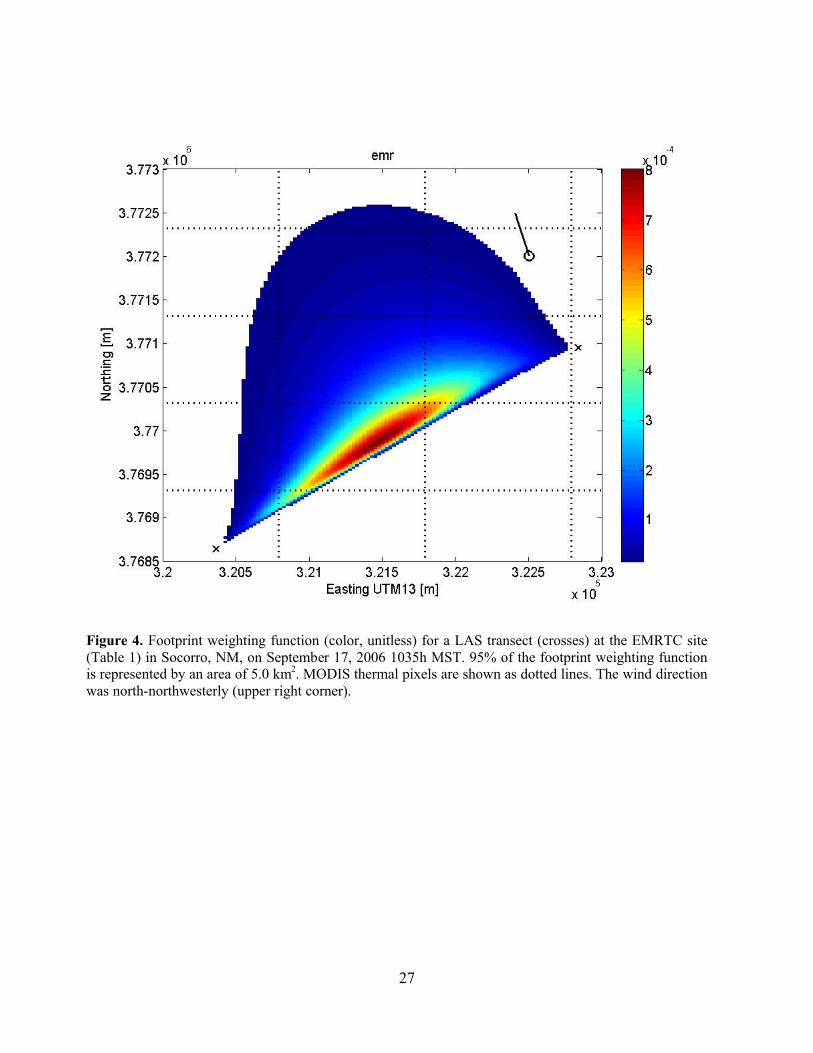
averaged measurements weighted towards the center of the transect (Fig. 4), the footprint typically
takes the shape of an ellipsoid whose major axis is ~30% less than the actual transect length. A
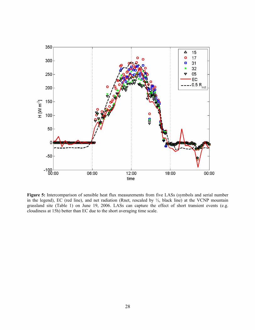
comparison of measurements from five collocated LAS transects and an eddy covariance station
reveal that LAS measurements follow the same trend as EC and capture better the effect of short
time transient events such as caused by scattered clouds (Fig. 5).
SCINTILLOMETER NETWORK IN NEW MEXICO
The scintillometer network in New Mexico (NMTLASNet) is located within and around the
Middle Rio Grande Basin. It consists of seven Kipp & Zonen LAS transects and associated
meteorological stations at different locations representing a range of elevations (1448 – 3206 m
MSL) and land surfaces: dry homogeneous shrub and grasslands, heterogeneous moist riparian
areas, moist homogeneous grassland, homogenous lava flows, and homogeneous irrigated alfalfa
fields (Table 1, Figures 6-7). The principal objectives for our current LAS network are: (1) Develop
efficient operating procedures and wireless infrastructure for the operation of LASs over a large
9
region; (2) Estimate typical footprint sizes and measurement errors of LAS observations (3)
Develop procedures for the use of H measurements by LASs for the calibration of remote sensing
algorithms.
Setup and Operating Procedures
The optimal transect is parallel to the earth’s surface and perpendicular to the predominant
wind direction to have a maximum uncorrelated source area. It should follow a north-south
orientation to avoid damage of the optical parts by direct sunlight under low sun angles. For typical
transects of 3 km the effect of the curvature of the earth on zeff is less than 0.2 m (Hartogensis et al.
2003). zeff should be within the atmospheric surface layer (ASL) where Monin-Obukhov Similarity
Theory (MOST) can be applied to derive H from CT2 (Eq. 2). The base of the ASL is two to three
times the typical height of the obstacles on the land surface (depending on the density of the
obstacles). Thus, the minimum zeff ranges from 1 m over grassland to tens of meters for trees. The
maximum height is the top of the ASL, which is on the order of 100 m in daytime, and 10s of
meters at night (Brutsaert 1982).
The minimum height is not only determined by the height of the roughness sublayer but also
by the phenomenon of “saturation”. When Cn2 increases above a certain threshold, σlnI
2 remains
constant (it is ‘saturated’) and is thus no longer proportional to Cn2. This violates the assumptions in
Eq. 1, and results in an underestimation of H (Clifford et al. 1974). Note that while H is constant in
the ASL, Cn2 decreases with height. Smaller zeff and longer transects lead to more intense
scintillations (larger σlnI2) and more saturation (Eq. 1). For example, to measure H = 400 W/m2 over
10
a path length of 2750 m, the height of the LAS must be greater than 30 m whereas H = 200 W/m2
would require a height of at least 10 m (Kipp&Zonen 2007).
Unlike with EC, the locations of LAS transmitter and receiver do not have to be
representative for the area under investigation as the measurement is most sensitive at the center of
the transect. Thus, to avoid the construction and vibration problems of tall towers, LASs can be set
up near the ground across a valley or between two hills. Where such landscape features cannot be
found vertically slanted paths can be used. Since LAS beam heights then vary along the path, the
LAS measurements not only represent a horizontal but also a vertical average of CT2. Table 1 shows
that with the exception of the Valles Caldera all our LAS transects have slanted paths where the
height difference exceeds 5 m. Advantages of slanted transects are reduction in installation cost and
flexibility. The disadvantage is an uncertainty in the derived H which increases with the ratio of
maximum to minimum height of the beam. While uncertainty in the physical height of the beam
over the transect can be eliminated by careful elevation measurements using differential GPS, the
uncertainty caused by different methods for determining the zeff remains. (Hartogensis et al. 2003).
Footprints of LAS measurements
For ground-truthing and data assimilation, it is essential to compare satellite or model results
to LAS measurements over identical areas. This includes estimating a footprint weighting function
of the flux measurement on the ground, summing up the footprint weights within each model grid
cell or remote sensing pixel, and computing the weighted average of the model or remote sensing H
values over the pixels comprising the footprint. Based on 13 daytime footprints (one example is
11
shown in Fig. 4), we found that the average footprint area 1 was 3.3 km2.
Several uncertainties plague footprint-averaged statistics: Firstly, footprint calculations are
based on turbulence models and use measurements with inherent uncertainty (e.g. wind direction).
Secondly, the temporal scale over which the remote sensing image is taken (seconds) is discrete and
different than the 10 minute average of the LAS measurement. Thirdly, subgrid-scale (or subpixel
scale) heterogeneity within the model gridcell or satellite image pixel is not considered. Subpixel-
scale heterogeneity becomes especially important when there is a strong gradient of footprint
weights within a pixel. Then the footprint-weighted pixel-averaged value from the LAS is not
representative for the relative weighting of the footprint area within that pixel.
Since the 1st issue is also affected by the 3rd (if H was homogeneous over the area
comprising the actual and the calculated footprint, then errors in the footprint location would not
matter) we examine the effect of subpixel-scale heterogeneity on the heat flux using Landsat-
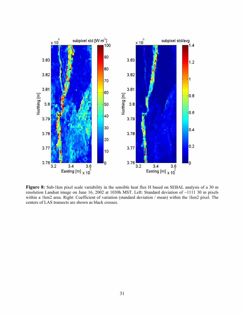
SEBAL H maps on June 16, 2002. Subpixel scale variability is related to features of the landscape
and cannot be described with purely statistical approaches (Fig. 8). For example, in the Rio Grande
riparian corridor, the river coexists with patches of riparian trees (e.g. Saltcedar and Cottonwood),
interdispersed shrubs and grasses, alfalfa fields, and bare, sandy or rocky soil on the edges
bordering the desert. This small-scale patchwork changes on scales much smaller than 1 km and
leads to significant subpixel-scale variability both in absolute (Fig. 8 left) and relative terms (Fig. 8
right). High subpixel scale variability also occurs at interfaces between different landscapes (so-
called ‘mixed pixels’), such as the dry riverbed of the Rio Puerco (upper left corner of the figure),
1 The footprint area is defined as the area that comprises 95% of the total footprint weight.
12
and the edge of the mountains (center right). In the desert area (northern half of Fig. 8) the absolute
subpixel scale variability is 10% or less.
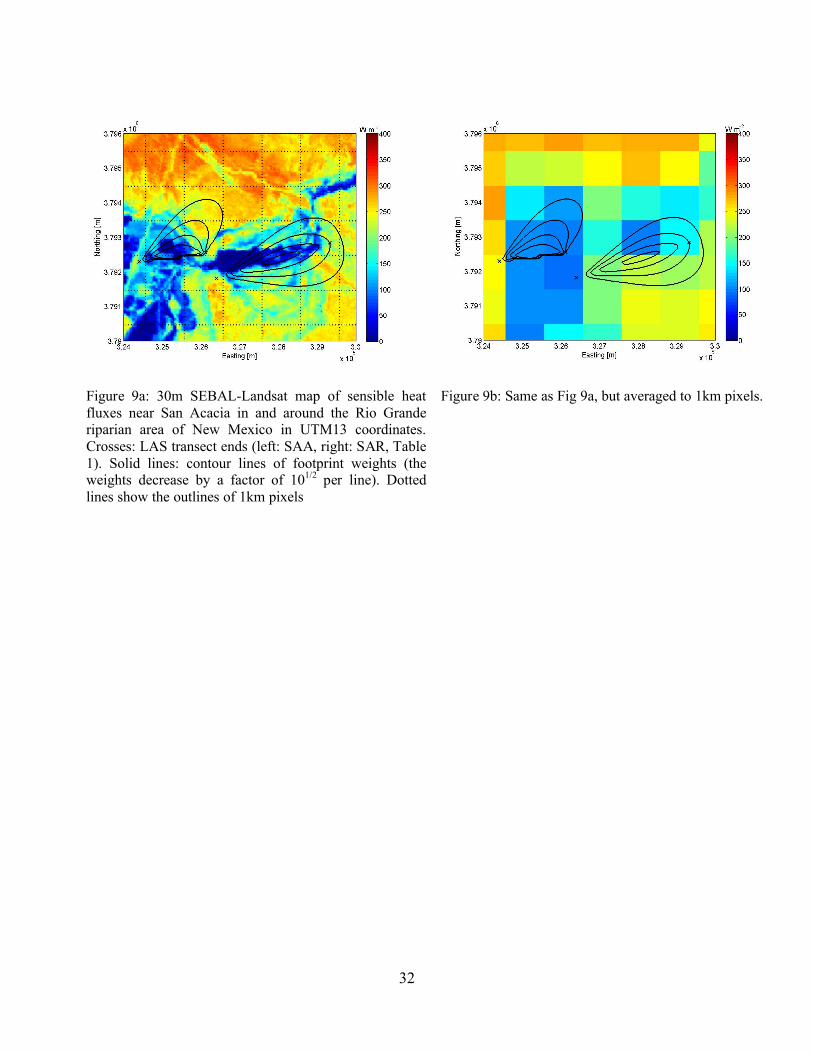
To quantify the effect of MODIS subpixel scale variability on validation and calibration of
remote sensing models, we applied the LAS footprint weighting functions on Sep 17, 2006 1040h
LST (the MODIS overpass time) to the 30 m pixel Landsat data (H30m, Fig 9a), and to the
aggregated 1 km pixel Landsat data (H1km, Fig. 9b). The Landsat scene covers 4 sites: San Acacia
Riparian (SAR), San Acacia Alfalfa (SAA), Sevilleta NWR desert, and EMRTC desert (Table 1).
For the more homogeneous desert sites, the differences in H30m and H1km are less than 3% (not
shown). However, for the SAR site H30m = 157 Wm-2 and H1km = 177 Wm-2, while we obtained H30m
= 96 Wm-2 and H1km = 171 Wm-2 for the SAA site (Fig. 9). While the difference between H30m and
H1km at SAR is acceptable, the error at SAA is 78%. From Fig 9b it is obvious that a substantial part
of the SAA footprint is over a ‘mixed pixel’ (the green pixel on the right), which covers partially
irrigated riparian area and partially a dry rocky hill. While the majority of the large weights in the
footprint are located over the riparian area (Fig. 9a), the mixed pixel artificially increases H1km for
the east end of the footprint, leading to overestimation of H1km .
LASs for the calibration and validation of remote sensing algorithms
The primary goal for our LAS network is calibration of the SEBAL remote sensing
algorithm to derive maps of sensible and latent heat fluxes over the state of New Mexico
operationally in near-real time. The required calibration of H to surface temperatures through user-
based selection of a ‘hot’ (with maximum sensible heat flux) and a ‘cold’ (with zero sensible heat
flux) pixel prevents automatic generation of these maps with SEBAL (Bastiaansen et al. 1998).
13
LAS sensible heat fluxes could be used to calibrate SEBAL surface temperature to H at the LAS
sites and then applied to the entire image.
To evaluate the accuracy of such a calibration procedure we compare SEBAL user-
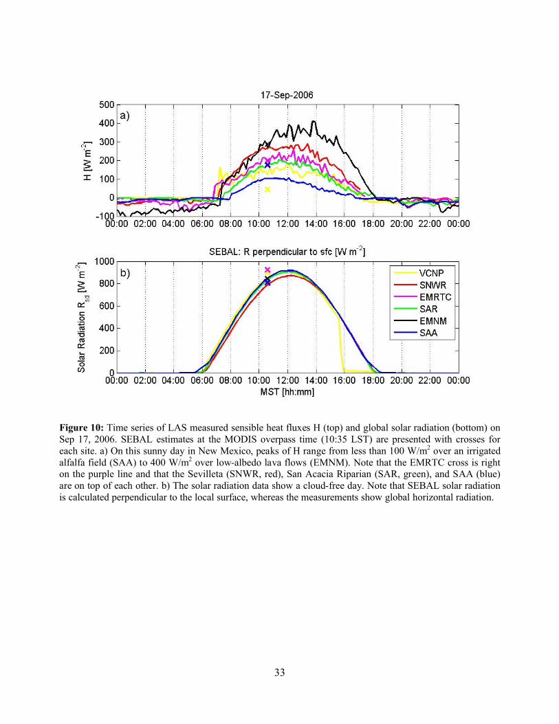
calibrated maps of H on September 17, 2006 (Fig. 10) and 3 other dates (Fig. 11). Figure 10 shows
that the SEBAL results generally agree with the 10 min averaged surface LAS measurements at the
overpass time, however, particularly the SAA, Sevilleta NWR desert, and VCNP estimates display
considerable errors. As discussed earlier, at SAA subpixel scale variability (Fig 9a) is probably
responsible for the error. The poor agreement between SEBAL and LAS at the more homogeneous
Sevilleta desert site is surprising and requires further research.
Application of SEBAL in the mountains (such as VCNP) is challenging. It is not clear yet
whether the difference between LAS and SEBAL there is caused by a biased SEBAL estimate of H,
erroneous estimate of the adiabatic lapse rate for the estimation of an elevation corrected surface
temperature in the high mountains, or errors in the ground measurements.
LESSONS LEARNED AND CONCLUSIONS
The installation of the NMTLASNet was completed in September 2006 (Table 1). We want
to share our “lessons learned” with colleagues who have an interest in employing the novel
technology of scintillometry.
The length of a LAS transect strongly depends on the height of the laser beam above the soil
surface and the expected maximum H. The commonly reported maximum transect length of 5000 m
for a LAS is overly optimistic for natural ecosystems. For New Mexico conditions with maximum

14
H>400 W/m2 a maximum transect length of 3000 m is more realistic if the beam height can be
maintained at 30 m. These lengths result in footprint areas which are not significantly larger than a
MODIS thermal pixel causing difficulties in comparison of LAS and satellite measurements in
heterogeneous environments. Downscaling MODIS 1km2 thermal pixels using 250x250 m MODIS
visible and near-infrared data would provide a better resolution for SEBAL calibration and
validation. However, transects over homogeneous areas are preferred as uncertainties in the
footprint model, meteorological data, and sub-1km-pixel scale variability can accumulate to
substantial errors.
From our extensive practical experience with LAS we can attest to the fact that they are
easier to operate and more robust than EC systems. Nevertheless new LAS users can avoid pitfalls
and become professional operators through training and guidance from an expert. Once a LAS is
setup, one site visit every two months is sufficient to service the instrument. Proper functionality
can be easily confirmed by observing a single variable – the receiver mean signal strength - that
may weaken due to power outages or sudden or creeping misalignment between transmitter and
receiver. For example, temporary installations on tripods, cinder blocks without a strong foundation
may cause misalignment problems to occur e.g. after heavy rainfall due to soil erosion or settling.
Misalignment increases the sensitivity of the measurements to tower vibrations which can introduce
additional variance in the signal strength leading to overprediction of H. LAS quality control can be
performed easily by a dedicated undergraduate student, whereas quality control of EC systems
typically requires the experience of an advanced PhD student. Scintillometer users should consult
the manual of their system for installation requirements, but generally a datalogger with the ability
for differential voltage measurements, a low bandwidth unidirectional data transmission system for
15
20 kB/day of uncompressed 10 minute averaged data, and 10W power system should suffice.
Unlike with EC systems, storage of high-frequency data is not required, but power spectra of the
signal strength may help in detecting vibration issues (van Radow et al. 2008).
It is somewhat more challenging to obtain the full diurnal cycle of H from an automatized
data processing algorithm. Since LASs measurements do not give information about the direction of
the flux, local minima in CT2 need to be found to determine the cross-over from negative to positive
and positive to negative heat fluxes around sunrise and sunset, respectively. Temperature
measurements at 2 heights can provide information about the direction of the flux more reliably,
especially over areas prone to horizontal advection of heat in the afternoon.
Lastly we would like to point out some disadvantages of LAS compared to EC. EC is based
on a simple theory to measure the fluxes directly. No additional specifications of the roughness of
the surface or the stability of the atmosphere are required. EC systems provide a greater wealth of
micrometeorological data than LASs such as velocity variances and momentum fluxes in all
directions. After more than 30 years of continuous and widespread use and development the
engineering of EC sensors is more advanced than that of LASs.
In summary, in New Mexico we have demonstrated how LAS networks can provide
valuable data for hydrologic modelers. We are in the process of optimizing our network based on
the experiences described in this paper and upscaling our network to the regional level (1000s km)
covering the southwestern USA and Latin America to investigate how scintillometry can contribute
to the validation and calibration of remote sensing algorithms, hydrologic models, and NWP.
Whereas in New Mexico evaporation is limited by water availability, in the humid tropics of
16
Panama and Colombia evaporation is limited by available energy except for short periods without
precipitation. Two LAS transects will be installed at the Gamboa Tropical Hydrology Observatory
(wet) and the “arcos seco” (dry arc) of Panama and one at an elevation of 2500 m in the highlands
surrounding Medellin, Colombia. We are actively looking for sponsors to cover the operating
expenses of the network and mesoscale meteorologists and hydrologist who would be interested in
the data for modeling or data assimilation.
ACKNOWLEDGEMENT
The following persons provided property or otherwise invaluable assistance in establishing
field sites: Jesus Gomez, Whitney Defoor, and Kimberly Bandy (all sites); Don Natvig and Renee
Brown (Sevilleta National Wildlife Refuge); Herschel Schulz (Chief Ranger, El Malpais National
Monument); Corky Herkenhoff and David Morris (San Acacia Alfalfa); Lorenzo Benavides (San
Acacia Riparian); Dan Klinglesmith (Magdalena Ridge); Bob Parmenter (Valles Caldera National
Preserve). The following sponsors have contributed to this study: USGS-NIWR USGS award
number 06HQGR0187 and NMSU-WRRI contract Q01112, NSF EPSCoR grant EPS-0447691;
U.S. Department of Agriculture, CSREES grant No.: 2003-35102-13654; NASA Cooperative
Agreement NNA06CN01A; the NSF Science and Technology Center program Sustainability of
Semi-Arid Hydrology and Riparian Areas (SAHRA; EAR-9876800).
17
REFERENCES
Allen, R.G., M. Tasumi, and R. Trezza, 2007, Satellite-based energy balance for mapping
evapotranspiration with internalized calibration (METRIC) – Model. J. Irrigation and Drainage
Engineering, 133 (4): 380-394.
Andreas, 1990, Selected Papers on Turbulence in a Refractive Medium. SPIE Milestone Series,
International Society for Optical Engineering, 25, 693 pp.
Anderson, M.C., J.M. Norman, J.R. Mecikalski, R.D. Torn, W.P. Kustas, and J.B. Basara. 2004. A
multi-scale remote sensing model for disaggregating regional fluxes to micrometeorological scales.
J. Hydrometeorology, 5, 343-363.
Bastiaanssen, W.G.M., M. Menenti, R.A. Feddes, and A.A. M. Holtslag. 1998, A remote sensing
surface energy balance algortithm for land (SEBAL). Part 1: Formulation. J. of Hydrology, 198-
212.
Beyrich, F., H.A.R. De Bruin, W.M.L. Meijninger, J.W. Schipper, and H. Lohse., 2002, Results
from one-year continuous operation of a large aperture scintillometer over heterogeneous land
surface. Bound.-Layer Meteorol., 105, 85-97.
Bou-Zeid E., C. Meneveau, M.B. Parlange, 2004, ‘Large-eddy simulation of neutral atmospheric
boundary layer flow over heterogeneous surfaces: Blending height and effective surface roughness,’
Water Resources Res., 40(W02505), doi:10.1029/2003WR002475.
Brutsaert W.H., 1982, Evapotranspiration into the Atmosphere, Theory, History and Applications,
Reidel Publising Co., Boston.
Choudhury, B.J., 1989, Estimating evaporation and carbon assimilation using infrared temperature
data: Vistas in modeling. In G. Asrar (Ed.), Theory and applications in optical remote sensing. John
Wiley, New York, pp. 628-690.
Clifford, S., G. Ochs, and R. Lawrence, 1974, Saturation of optical scintillation by strong
turbulence. J. Opt. Soc. Am., 64, 148– 154.
De Bruin, H.A.R., 2001, Introduction: Renaissance of Scintillometry, Boundary-Layer Meteorol.,
105(1), 1-4.
De Bruin, H.A.R., W. Kohsiek, and B.J.J.M. Van den Hurk, ‘A Verification of Some Methods to
Determine the Fluxes of Momentum, Sensible Heat and Water Vapour using Standard Deviation
18
and Structure Parameter of Scalar Meteorological Quantities’, Boundary-Layer Meteorol. 63, 231-
257, 1993
Foken, T., F. Wimmer, M. Mauder, C. Thomas, and C. Liebethal, 2006, Some aspects of the energy
balance closure problem, Atmos. Chem. Phys. Discuss., 6, 3381–3402.
Goodrich D.C., R. Scott, J. Qi, B. Goff, C. L. Unkrich, M. S. Moran, D. Williams, S. Schaeffer, K.
Snyder, R. MacNish, T. Maddock, D. Pool, A. Chehbouni, D. I. Cooper, W. E. Eichinger, W. J.
Shuttleworth, Y. Kerr, R. Marsett and W. Nil, 2000, Seasonal estimates of riparian
evapotranspiration using remote and in-situ measurements, Agric. Forest Meteorol., 105(1-3), 281-
309.
Hartogensis, O.K., C. J. Watts, J.-C. Rodriguez, H.A.R. De Bruin, 2003, Derivation of effective
height for scintillometers: La Poza experiment in Northwest Mexico. J. Hydrometeorology, 4, 915-
929
Hendrickx, J.M.H., and S.-H. Hong. 2005, Mapping sensible and latent heat fluxes in arid areas
using optical imagery. Proc. International Society for Optical Engineering, SPIE 5811:138-146.
Hill, R.J., 1992, Review of optical scintillation methods of measuring the refractive-index spectrum,
inner scale and surface fluxes. Waves in Random Media, 2, 179-201
Hong, S. 2008. Mapping regional distributions of energy balance parameters using optical remotely
sensed imagery. Ph.D. Dissertation, New Mexico Tech, Socorro NM.
Horst, T.W. and J.C. Weil. 1992, Footprint Estimation for Scalar Flux Measurements in the
Atmospheric Surface Layer. Bound.-Layer Meteorology. 59: 279-296.
Hsieh, C.-I., G. Katul, and T.-W. Chi, 2000, An approximate analytical model for footprint
estimation of scalar fluxes in thermally stratified atmospheric flows. Adv. Water Res., 23, 765-772.
Janjic, Z. L., 2004: The NCEP WRF core. Preprints, 20th Conference on Weather Analysis and
Forecasting/16th Conference on Numerical Weather Prediction, Seattle, WA, Amer. Meteor. Soc.,
on CD-ROM
Katul, G., C.-I. Hsieh, D. Bowling, K. Clark, N. Shurpali, A. Turnipseed, J. Albertson, K. Tu, D.
Hollinger, B. Evans, B. Offerle, D. Anderson, D. Ellsworth, C. Vogel, and R. Oren, 1999: Spatial
variability of turbulent fluxes in the roughness sublayer of an even-aged pine forest. Bound.-Layer
Meteorol., 93, 1–28.
Kipp & Zonen, 2007, Large Aperture Scintillometer Instruction Manual
19
Kleissl, J., J. Gomez, S.-H. Hong, K. Fleming, J.M.H. Hendrickx, T. Rahn, 2008, Large Aperture
Scintillometer Intercomparison Study. Bound.-Layer Meteorol., in press.
Kustas, W.P. and J.M. Norman. 1996, Use of remote sensing for evapotranspiration monitoring
over land surfaces. Hydrol. Science J., 41, 495-515.
Lee, X. (Ed.), Massman W. (Ed), Law B. (Ed), 2004, Handbook of Micrometeorology: A Guide for
Surface Flux Measurement and Analysis (Atmospheric and Oceanographic Sciences Library).
Kluwer Academic Publishers, The Netherlands.
Loescher, H., T. Ocheltree, B. Tanner, E. Swiatek, B. Dano, J. Wong, G. Zimmerman, J. Campbell,
C. Stock, L. Jacobsen, Y. Shiga, J. Kollas, J. Liburdy, and B. Law, 2005, Comparison of
temperature and wind statistics in contrasting environments among different sonic anemometer-
thermometers. Agricultural Forest Meteorol., 133, 119–139
Meijninger, W., O. Hartogensis, W. Kohsiek, J. Hoedjes, R. Zuurbier, and H. de Bruin, 2002:
Determination of area averaged sensible heat fluxes with a large aperture scintillometer over a
heterogeneous surface - Flevoland field experiment. Bound.-Layer Meteorol., 105, 63-83
Middle Rio Grande Water Assembly. 1999. Middle Rio Grande water budget (where water comes
from, and goes, and how much): averages for 1972-1997. Middle Rio Grande Council of
Governments of New Mexico. 10 pages.
Moran, S.M., and R.D. Jackson. 1991. Assessing the spatial distribution of evaporation using
remotely sensed inputs. J. Environ. Qual., 20, 725-737.
Panofsky, H. and J. Dutton, 1984: Atmospheric Turbulence. John Wiley & Sons, New York.
Peters Lidard, C.D., S. Kumar, Y. Tian, J.L. Eastman, and P. Houser. 2004. Global urban-scale
land-atmosphere modeling with the land information system. 84th AMS Annual Meeting 11-15
January 2004, Symposium on Planning, Nowcasting, and Forecasting in the Urban Zone.
Scintec, 2004, Boundary Layer Scintillometer: Turbulence, Heat Flux, Crosswind over Large
Spatial Scales, http://www.scintec.com/Site.1/turb.htm
Schmid, H.P. and T.R. Oke. 1990, A model to estimation the source area contributing to turbulent
exchange in the surface layer over patchy terrain. Q.J.R. Meteorol. Soc., 116, 965-988.
Schuepp P.H., M.Y. Leclerc, J.I. MacPherson, and R.L. Desjardins, 1990, Footprint prediction of
scalar fluxes from analytical solutions of the diffusion equation, Bound.-Layer Meteorol., 50, 355-
373
20
Song, J., M. L. Wesely, R. L. Coulter, and E. A. Brandes, 2000, Estimating watershed
evapotranspiration with PASS. Part I: Inferring root-zone moisture conditions using satellite data. J.
Hydrometeorol., 1, 447–461.
Twine TE, WP Kustas, JM Norman, DR Cook, PR Houser, TP Meyers, JH Prueger, PJ Starks,
2000, Correcting eddy covariance flux underestimates over a grassland. Agric. For. Meteor, 103,
279-300
Von Randow C., B. Kruijt, A.A.M. Holtslag, M.B.L. de Oliveira, 2008, Exploring eddy-covariance
and large-aperture scintillometer measurements in an Amazonian rain forest, Agricultural and
Forest Meteorology, 148, 680-690
Wilson, K., A. Goldstein, E. Falge, M. Aubinet, D. Baldocchi, P. Berbigier, C. Bernhofer,
R. Ceulemans, H. Dolmanh, C. Field, A. Grelle, A. Ibrom, B. Lawl, A. Kowalski, T.Meyers,
J. Moncrieff, R. Monsonn, W. Oechel, J. Tenhunen, R. Valentini, and S. Verma, 2002. Energy
balance closure at FLUXNET sites. Agric. For. Meteorol., 113, 223–243.
21
FIGURE AND TABLE CAPTIONS
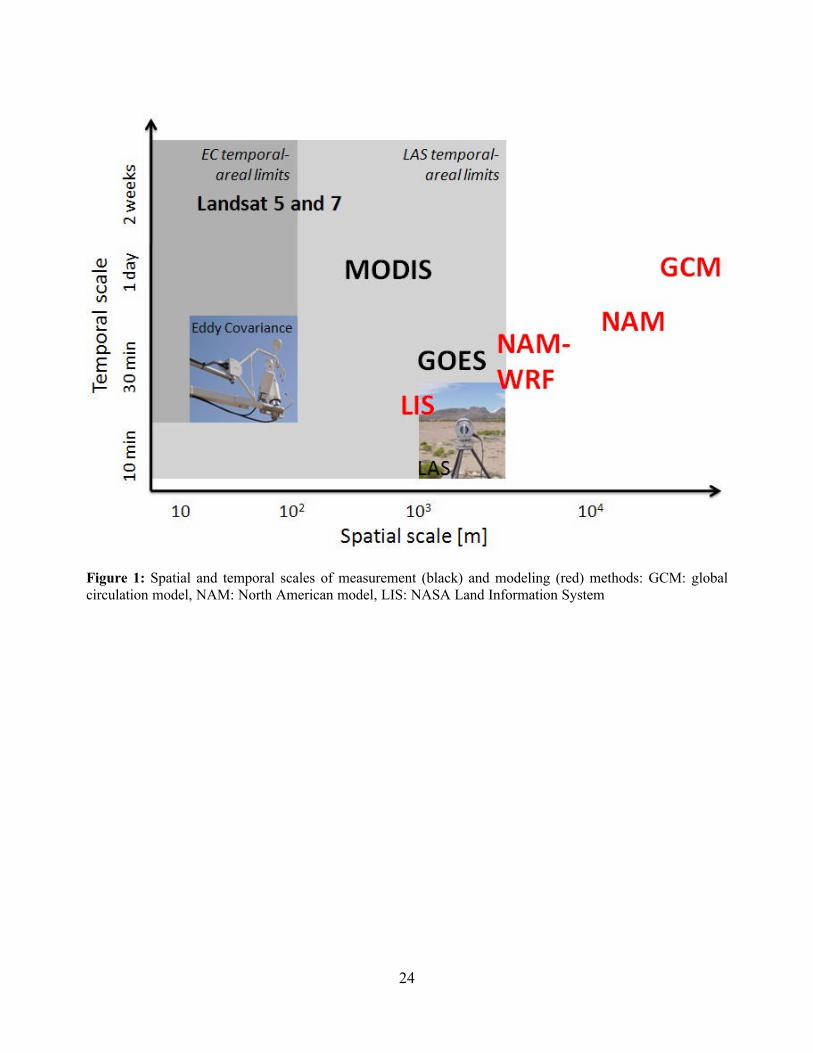
Figure 1: Spatial and temporal scales of measurement (black) and modeling (red) methods: GCM:
global circulation model, NAM: North American model, LIS: NASA Land Information System
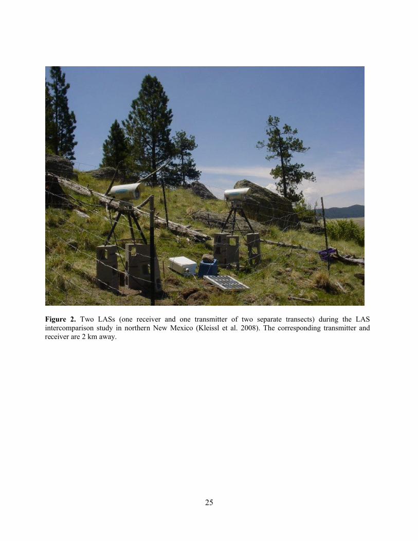
Figure 2: Two LASs (one receiver and one transmitter of two separate transects) during the LAS
intercomparison study in northern New Mexico (Kleissl et al., 2008). The corresponding transmitter
and receiver are 2 km away.
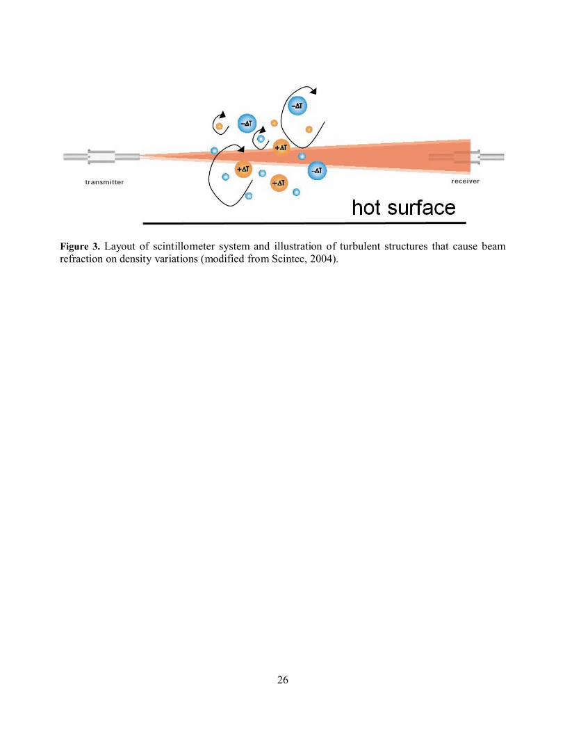
Figure 3: Layout of scintillometer system and illustration of turbulent structures that cause beam
refraction on density variations (modified from Scintec, 2004).
Figure 4: Footprint weighting function (color, unitless) for a LAS transect (crosses) at the EMRTC
site (Table 1) in Socorro, NM, on September 17, 2006 1035h MST. 95% of the footprint weighting
function is represented by an area of 5.0 km2. MODIS thermal pixels are shown as dotted lines.
Figure 5: Intercomparison of sensible heat flux measurements from five LASs (symbols and serial
number in the legend), EC (red line), and net radiation (black line) at the VCNP mountain grassland
site (Table 1) on June 19, 2006. LASs can capture the effect of short transient events (e.g.
cloudiness at 15h) better than EC due to the short averaging time scale.
22
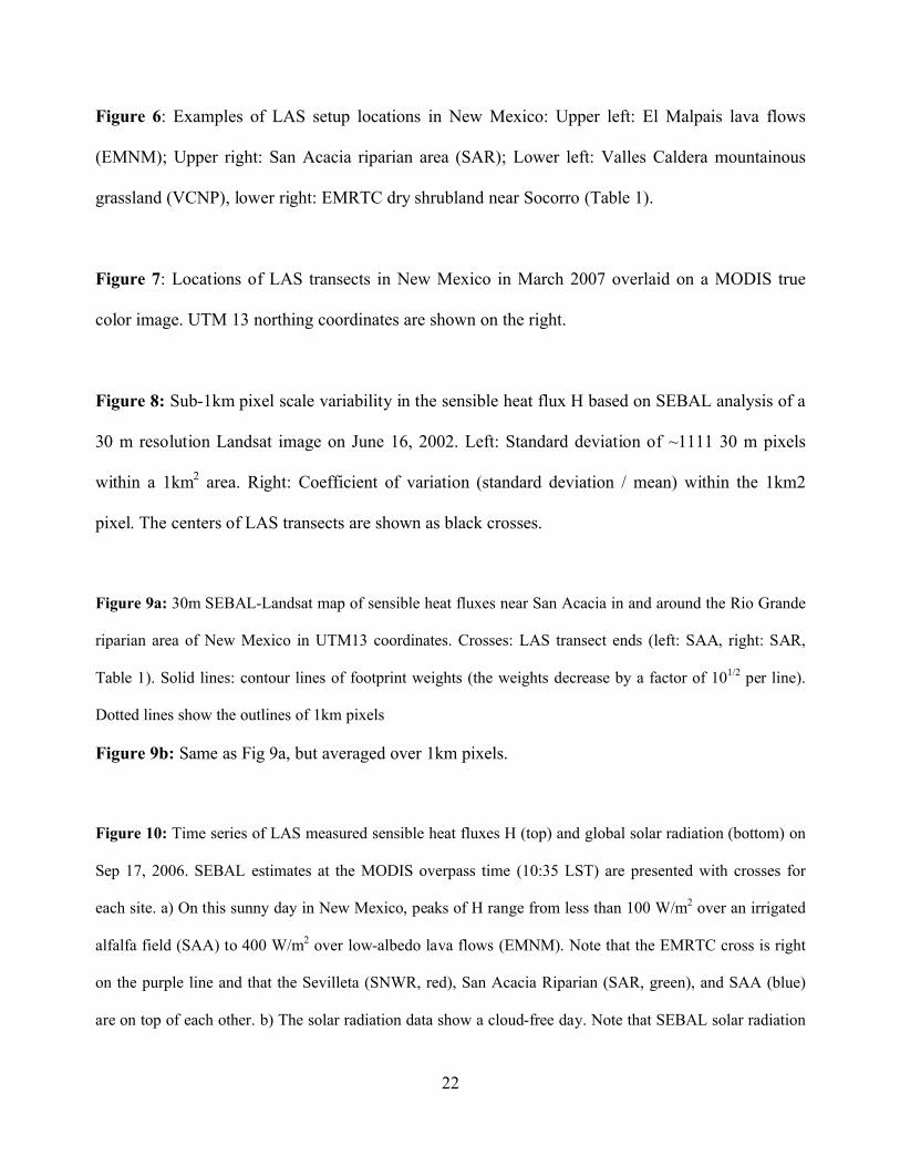
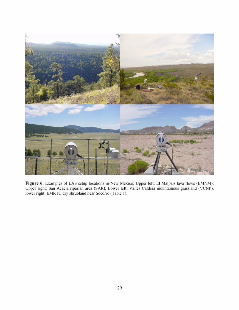
Figure 6: Examples of LAS setup locations in New Mexico: Upper left: El Malpais lava flows
(EMNM); Upper right: San Acacia riparian area (SAR); Lower left: Valles Caldera mountainous
grassland (VCNP), lower right: EMRTC dry shrubland near Socorro (Table 1).
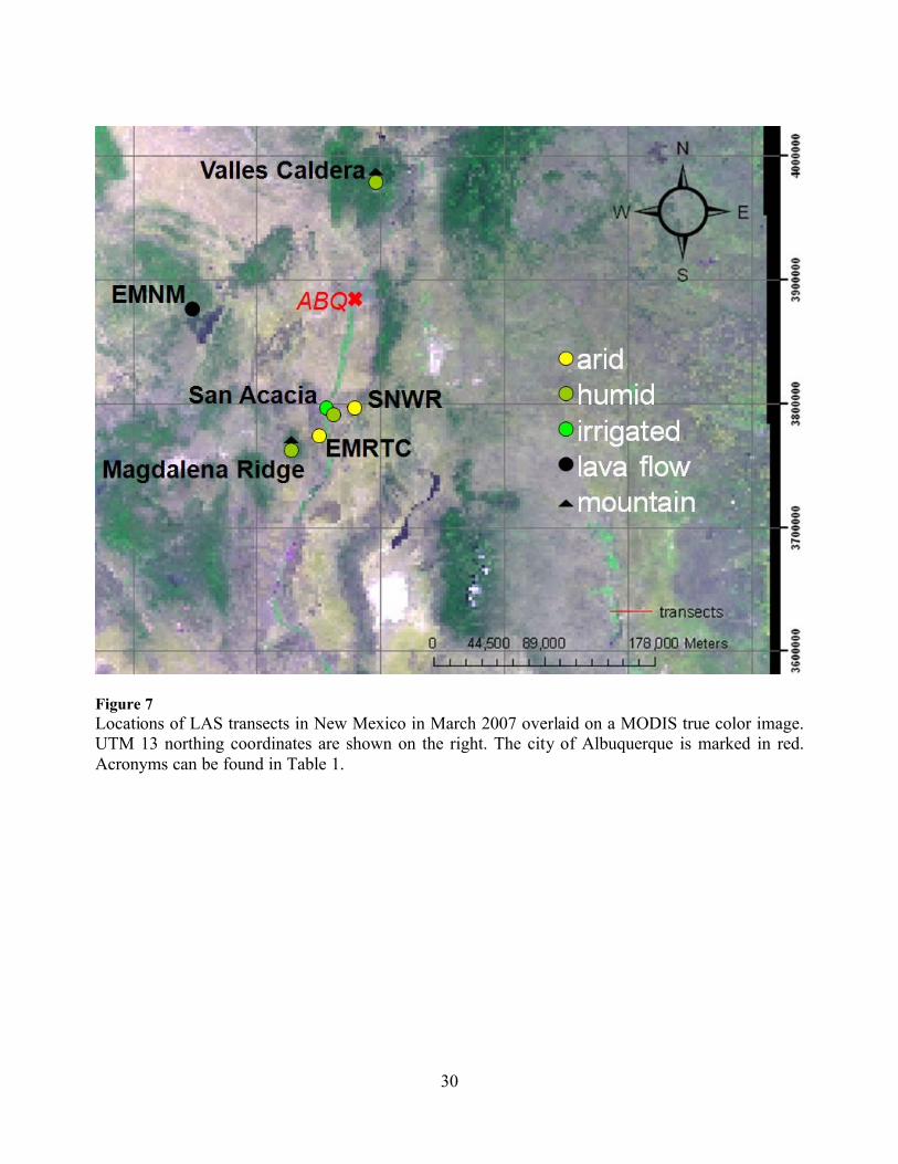
Figure 7: Locations of LAS transects in New Mexico in March 2007 overlaid on a MODIS true
color image. UTM 13 northing coordinates are shown on the right.
Figure 8: Sub-1km pixel scale variability in the sensible heat flux H based on SEBAL analysis of a
30 m resolution Landsat image on June 16, 2002. Left: Standard deviation of ~1111 30 m pixels
within a 1km2 area. Right: Coefficient of variation (standard deviation / mean) within the 1km2
pixel. The centers of LAS transects are shown as black crosses.
Figure 9a: 30m SEBAL-Landsat map of sensible heat fluxes near San Acacia in and around the Rio Grande
riparian area of New Mexico in UTM13 coordinates. Crosses: LAS transect ends (left: SAA, right: SAR,
Table 1). Solid lines: contour lines of footprint weights (the weights decrease by a factor of 101/2 per line).
Dotted lines show the outlines of 1km pixels
Figure 9b: Same as Fig 9a, but averaged over 1km pixels.
Figure 10: Time series of LAS measured sensible heat fluxes H (top) and global solar radiation (bottom) on
Sep 17, 2006. SEBAL estimates at the MODIS overpass time (10:35 LST) are presented with crosses for
each site. a) On this sunny day in New Mexico, peaks of H range from less than 100 W/m2 over an irrigated
alfalfa field (SAA) to 400 W/m2 over low-albedo lava flows (EMNM). Note that the EMRTC cross is right
on the purple line and that the Sevilleta (SNWR, red), San Acacia Riparian (SAR, green), and SAA (blue)
are on top of each other. b) The solar radiation data show a cloud-free day. Note that SEBAL solar radiation

23
is calculated perpendicular to the local surface, whereas the measurements show global horizontal radiation.
Figure 11: Scatter plot of LAS and SEBAL sensible heat fluxes at six sites (Table 1) and four
satellite overpasses in 2006. The legend shows month, day, and site name.
24
Figure 1: Spatial and temporal scales of measurement (black) and modeling (red) methods: GCM: global circulation model, NAM: North American model, LIS: NASA Land Information System
25
Figure 2. Two LASs (one receiver and one transmitter of two separate transects) during the LAS intercomparison study in northern New Mexico (Kleissl et al. 2008). The corresponding transmitter and receiver are 2 km away.
26
Figure 3. Layout of scintillometer system and illustration of turbulent structures that cause beam refraction on density variations (modified from Scintec, 2004).
27
Figure 4. Footprint weighting function (color, unitless) for a LAS transect (crosses) at the EMRTC site (Table 1) in Socorro, NM, on September 17, 2006 1035h MST. 95% of the footprint weighting function is represented by an area of 5.0 km2. MODIS thermal pixels are shown as dotted lines. The wind direction was north-northwesterly (upper right corner).
28
Figure 5: Intercomparison of sensible heat flux measurements from five LASs (symbols and serial number in the legend), EC (red line), and net radiation (Rnet, rescaled by ½, black line) at the VCNP mountain grassland site (Table 1) on June 19, 2006. LASs can capture the effect of short transient events (e.g. cloudiness at 15h) better than EC due to the short averaging time scale.
29
Figure 6: Examples of LAS setup locations in New Mexico: Upper left: El Malpais lava flows (EMNM); Upper right: San Acacia riparian area (SAR); Lower left: Valles Caldera mountainous grassland (VCNP), lower right: EMRTC dry shrubland near Socorro (Table 1).
30
Figure 7Locations of LAS transects in New Mexico in March 2007 overlaid on a MODIS true color image. UTM 13 northing coordinates are shown on the right. The city of Albuquerque is marked in red. Acronyms can be found in Table 1.
31
Figure 8: Sub-1km pixel scale variability in the sensible heat flux H based on SEBAL analysis of a 30 m resolution Landsat image on June 16, 2002 at 1030h MST. Left: Standard deviation of ~1111 30 m pixels within a 1km2 area. Right: Coefficient of variation (standard deviation / mean) within the 1km2 pixel. The centers of LAS transects are shown as black crosses.
32
Figure 9a: 30m SEBAL-Landsat map of sensible heatfluxes near San Acacia in and around the Rio Grande riparian area of New Mexico in UTM13 coordinates. Crosses: LAS transect ends (left: SAA, right: SAR, Table 1). Solid lines: contour lines of footprint weights (the weights decrease by a factor of 101/2 per line). Dotted lines show the outlines of 1km pixels
Figure 9b: Same as Fig 9a, but averaged to 1km pixels.
33
Figure 10: Time series of LAS measured sensible heat fluxes H (top) and global solar radiation (bottom) onSep 17, 2006. SEBAL estimates at the MODIS overpass time (10:35 LST) are presented with crosses for each site. a) On this sunny day in New Mexico, peaks of H range from less than 100 W/m2 over an irrigatedalfalfa field (SAA) to 400 W/m2 over low-albedo lava flows (EMNM). Note that the EMRTC cross is right on the purple line and that the Sevilleta (SNWR, red), San Acacia Riparian (SAR, green), and SAA (blue) are on top of each other. b) The solar radiation data show a cloud-free day. Note that SEBAL solar radiation is calculated perpendicular to the local surface, whereas the measurements show global horizontal radiation.

34
Figure 11: Scatter plot of LAS and SEBAL sensible heat fluxes at six sites (Table 1) and four satellite overpasses in 2006. The legend shows month, day, and site name.
35
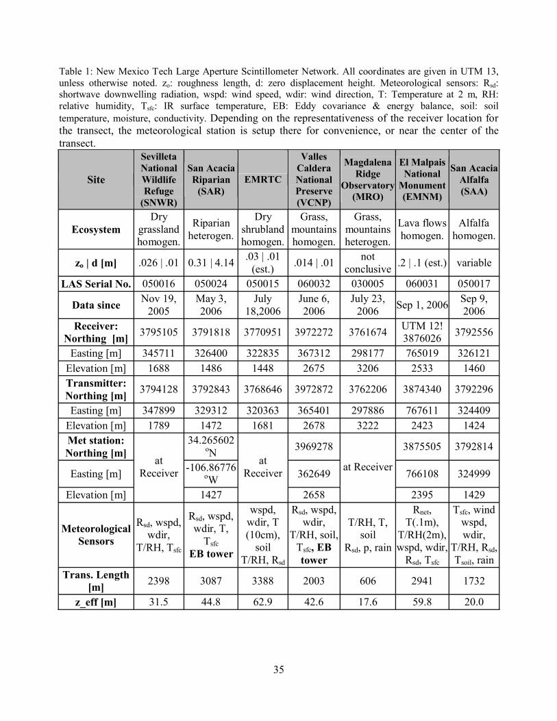
Table 1: New Mexico Tech Large Aperture Scintillometer Network. All coordinates are given in UTM 13, unless otherwise noted. zo: roughness length, d: zero displacement height. Meteorological sensors: Rsd: shortwave downwelling radiation, wspd: wind speed, wdir: wind direction, T: Temperature at 2 m, RH: relative humidity, Tsfc: IR surface temperature, EB: Eddy covariance & energy balance, soil: soil temperature, moisture, conductivity. Depending on the representativeness of the receiver location for the transect, the meteorological station is setup there for convenience, or near the center of the transect.
Site
Sevilleta National Wildlife Refuge
(SNWR)
San AcaciaRiparian
(SAR)EMRTC
Valles Caldera National Preserve(VCNP)
Magdalena Ridge
Observatory (MRO)
El Malpais National
Monument (EMNM)
San AcaciaAlfalfa(SAA)
EcosystemDry
grasslandhomogen.
Riparianheterogen.
Dry shrublandhomogen.
Grass, mountainshomogen.
Grass, mountainsheterogen.
Lava flowshomogen.
Alfalfahomogen.
zo | d [m] .026 | .01 0.31 | 4.14 .03 | .01 (est.) .014 | .01 not
conclusive .2 | .1 (est.) variable
LAS Serial No. 050016 050024 050015 060032 030005 060031 050017
Data since Nov 19, 2005
May 3, 2006
July 18,2006
June 6, 2006
July 23, 2006 Sep 1, 2006 Sep 9,
2006Receiver:
Northing [m] 3795105 3791818 3770951 3972272 3761674 UTM 12!3876026 3792556
Easting [m] 345711 326400 322835 367312 298177 765019 326121Elevation [m] 1688 1486 1448 2675 3206 2533 1460Transmitter: Northing [m] 3794128 3792843 3768646 3972872 3762206 3874340 3792296
Easting [m] 347899 329312 320363 365401 297886 767611 324409Elevation [m] 1789 1472 1681 2678 3222 2423 1424Met station: Northing [m]
34.265602oN 3969278 3875505 3792814
Easting [m] -106.86776oW 362649 766108 324999
Elevation [m]
at Receiver
1427
at Receiver
2658
at Receiver
2395 1429
Meteorological Sensors
Rsd, wspd, wdir,
T/RH, Tsfc
Rsd, wspd, wdir, T,
TsfcEB tower
wspd, wdir, T (10cm),
soilT/RH, Rsd
Rsd, wspd, wdir,
T/RH, soil, Tsfc, EB tower
T/RH, T, soil
Rsd, p, rain
Rnet, T(.1m),
T/RH(2m),wspd, wdir,
Rsd, Tsfc
Tsfc, windwspd, wdir,
T/RH, Rsd, Tsoil, rain
Trans. Length [m] 2398 3087 3388 2003 606 2941 1732
z_eff [m] 31.5 44.8 62.9 42.6 17.6 59.8 20.0
Related Documents