New implementation techniques of an efficient MPEG advanced audio coder

E. Kurniawati et al.: New Implementation Techniques of an Efficient MPEG Advanced Audio Coder

Contributed Paper Manuscript received February 16, 2004 0098 3063/04/$20.00 © 2004 IEEE

655

New Implementation Techniques of an Efficient MPEG Advanced Audio Coder

E. Kurniawati, C. T. Lau, B. Premkumar, J. Absar, S. George

Abstract — MPEG-AAC is the current state of the art in audio compression technology. The CD-quality promised at bit rate as low as 64 kbps makes AAC a strong candidate for high quality low bandwidth audio streaming applications over wireless network. Besides this low bit rate requirement, the codec must be able to run on personal wireless handheld devices with its inherent low power characteristics. While the AAC standard is definite enough to ensure that a valid AAC stream is correctly decodable by all AAC decoders, it is flexible enough to accommodate variations in implementation, suited to different resources available and application areas. This paper reviews various implementation techniques of the encoder. We then proposed our method of an optimized software implementation of MPEG-AAC (LC profile). The coder is able to perform encoding task using half the processing power compared to standard implementation without significant degradation in quality as shown by both subjective listening test and an ITU-R compliant quality testing program (OPERA).

Index Terms — Audio Compression, MPEG-AAC, Psychoacoustics Model, Quantization.

I. INTRODUCTION

Audio technology has evolved tremendously over the last century. In the advent of digital systems, sound reproduction reaches its state of the art performance in terms of quality. However, the high bit rate characteristic of digital music does not suit the demand of application with limited bandwidth, for example, in digital audio streaming. To achieve efficient transmission, compression needs to be employed.

Efficient coding systems are those that could optimally eliminate irrelevant and redundant parts of an audio stream. The first is achieved by reducing psychoacoustical irrelevancy through psychoacoustics analysis. The term “perceptual audio coder” was coined to refer to those compression schemes that exploit the properties of human auditory perception. Further reduction is obtained from redundancy reduction.

This work was supported by ST Microelectronics Asia Pacific Pte Ltd. E.Kurniawati, C.T. Lau, and B. Premkumar are with School of Computer

Engineering, Nanyang Technological University, Nanyang Avenue, Singaproe 639798(email: [email protected], [email protected], [email protected]).

J.Absar and S. George are with ST Microelectronics Asia Pacific Pte. Ltd., R&D Centre Singapore Science Park II, Teletech Park, Singapore (e-mail: [email protected], [email protected]).

Among the perceptual audio coding schemes available today, MPEG-AAC is the leading option, giving transparent CD quality at 64kbps. In this scheme, each AAC frame is independently decodable. With time domain aliasing cancellation concept, the information is carried by two consecutive AAC frames. These features make the scheme favourable when it comes to audio streaming application.

The recent advances in wireless network bring about the challenge of developing applications on portable devices, including digital audio streaming. Not only low bit rate is desired, but also the encoder and decoder pair must be able to run on this low power portable device. These are the motivations behind our research.

The AAC decoder is less demanding computationally, particularly because of the lack of psychoacoustics and bit allocations modules. These two modules will be the focus of our discussion. Section 2 will give a brief description of AAC and its efficiency issues. Section 3 will discuss psychoacoustics and time to frequency transformation in greater detail and section 4 will focus on bit allocation-quantization module. Finally, section 5 will highlight the experimental results and conclusion will be presented in section 6.

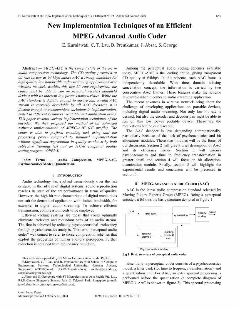
II. MPEG-ADVANCED AUDIO CODER (AAC) AAC is the latest audio compression standard released by

Moving Picture Experts Group (MPEG). Being a perceptual encoder, it follows the basic structure depicted in figure 1

filter bank quantisationentropycoding

maskingthreshold

calc.

spectralanalysis

input

Psychoacoustics module

output

Fig 1. Basic structure of perceptual audio coder

Essentially, a perceptual coder consists of a psychoacoustics

model, a filter bank (for time to frequency transformation), and a quantization unit. For AAC, an extra spectral processing is performed before the quantization (a complete diagram of MPEG-4 AAC is shown in figure 2). This spectral processing

IEEE Transactions on Consumer Electronics, Vol. 50, No. 2, MAY 2004

block is used to reduce redundant components, consisting mostly of prediction tools.

AAC uses Modified Discrete Cosine Transform (MDCT) with 50% overlap in its filterbank module. After overlap-add process, due to the time domain aliasing cancellation, we should be able to get a perfect reconstruction of the original signal. However, this is not the case because error is introduced during the quantization process. The idea of a perceptual coder is to hide this quantization error such that our hearing will not notice it. Those spectral components that we would not be able to hear are also eliminated from the coded stream. This irrelevancy reduction exploits the masking properties of human ear (more details on this will be given in subsequent section). The quality of a perceptual coder depends on the psychoacoustics module because this is where all the psychoacoustical analysis is performed. The calculation of masking threshold is among the computationally intensive task of the encoder.

AAC has 2 different window sizes to be used depending on whether the signal is stationary or transient. This feature combats the pre-echo artifact, which all perceptual encoders are prone to. The decision to switch between window sizes is also determined by the psychoacoustics module, making it more crucial to the performance of the encoder.

AAC quantization module operates in two-nested loop. The inner loop quantizes the input vector and increases the quantizer step size until the output vector can be coded with the available number of bits. After completion of the inner loop an outer loop checks the distortion of each scale factor band and, if the allowed distortion is exceeded, amplifies the scale factor band and calls the inner loop again. AAC uses a non-uniform quantizer.

Figure 2 shows the complete diagram of MPEG4-AAC [1]. There are 3 profiles defined in the standard:

- Main Profile, with all the tools enabled demanding substantial processing power.

- Low Complexity (LC) Profile, with lesser compression ratio to save processing and RAM usage

- Scaleable Sampling Rate Profile, with ability to adapt to various bandwidths.

We will discuss only the second profile as processing power savings is our main concern.

Besides the main module explained earlier, AAC-LC has Temporal Noise Shaping (TNS) and stereo coding enabled without the rest of the prediction module in the spectral processing unit (please refer to figure 2). Working in tandem with block switching, TNS is also used to reduce the pre-echo artefact by controlling the temporal shape of the quantization noise. However, in LC profile the order of TNS is limited. The stereo coding is used to control the imaging of coding noise by coding the left and right coefficients as sum and difference.

The AAC standard only ensures that a valid AAC stream is correctly decodable by all AAC decoders. The encoder can accommodate variations in implementation, suited to different resources available and application areas. AAC-LC is the

profile tiled to have lesser computational burden compared to the other profiles. However, the overall efficiency still depends on the detail implementations of the encoder itself.

AAC GainControl Tool

FilterBank

BitstreamFormatter

Psychoacoustic Model

14496-3Coded

Audio Stream

Inputtime

signal

WindowLength

Decision

Perceptualmodel

Bark Scaleto

ScalefactorBand

Mapping

TNS

Intensity/Coupling

Prediction

M/S

PNS

LTP

Spectral Processing

Spectrumnormalization and

Interleaved VQ

Scalefactorcoding

QuantizationNoiseless coding

Quantization and Coding

AAC Twin VQ

Fig 2. Block diagram of MPEG4-AAC

Figure 3 shows the computational demand of a standard

AAC-LC implementation from MPEG reference coder, run for 64 kbps bit rate with CD quality sampling rate of 44.1 kHz. Psychoacoustics module takes up 22% of the processing power due to its heavy spectral analysis for the masking threshold calculation. The most demanding module is quantization due to the presence of the nested loop for rate distortion control. These are the 2 modules that have been of interest in the effort to optimize the encoder.

In this paper, we will describe these two modules and various options for their implementation to improve the efficiency along with the pros and cons. Sufficient arguments will be presented before choosing the final method and a comparison will be performed with the initial implementation in terms of both computation and subjective quality.

Psychoacoustics (22%)

Filterbank(5%)

Quantization(64%)

Other(9%)

Fig 3. Distribution of resources in AAC-LC encoder

656

E. Kurniawati et al.: New Implementation Techniques of an Efficient MPEG Advanced Audio Coder 657

III. PSYCHOACOUSTICS AND FILTERBANK A perceptual audio coder achieves compression by reducing

psychoacoustical irrelevancy in the audio data stream. The masking threshold is determined to judge which part of the signal is less important to our perception. This is done by exploiting simultaneous masking properties of our auditory system, which states that under the influence of one prominent tone, the adjacent spectral components will lose their significance to our perception.

The main steps in calculating the masking threshold in the Psychoacoustics Module (PAM) are summarized as follows:

1. Transformation to frequency domain.

To calculate the complex spectrum of the input signal, an FFT is performed on the windowed (Hann window) segment of the input signal, resulting in spectral coefficient X(k):

∑−

=

−− ==

1

0

2)( )(1)()(

N

n

Nnkj

kj enxN

ekrkXπ

θ

2. Calculation of the energy spectrum

The spectral coefficients are segmented into seventy partitions [1] and the energy for each segment is computed, as below:

∑=

=)(

)(

2 )()(bkhigh

bklowkkrbe

where klow and khigh are the lowest and highest frequency line in the partition, and b is the partition index.

3. Convolution with the spreading functions. This step accounts for the spread of the masking phenomenon across critical (or bark) bands. An analytical expression for the spreading function (for each partition) is given by:

where x represents the distance (in bark) of the masker from the maskee. This gives us a triangular model for spreading function with slopes of +25 and –10 dB per bark. Observe in Fig. 4 that the masking effect is gently sloping on the higher frequency end while on the lower side it is considerably steep. This accounts for the fact that it is easier to mask higher frequency component than the lower ones.

4. Determination of the tonality index

Tonals and noise have different masking capabilities (the later being a better masker). A precise assessment of tonality is crucial in order to avoid under-coding and over-coding. In AAC, this parameter is estimated using unpredictability measure. Here, let Xp(k) be the predicted value for coefficient X(k). Xp(k) is computed by extrapolating values of X(k) over the previous two frames. A

measure of unpredictability is computed as shown below:

u(k)=|X(k) – Xp(k) | / ( |X(k)|+|Xp(k)| ) which is essentially a ratio of the prediction-error to the magnitude of the coefficient and its predicted value. The weighted unpredictability is determined by multiplying the energy r2(k) with the unpredictability measure u(k), and summing the product over each partition. A convolution of the sum is then performed with the spreading function. Since this result is weighted by the signal energy, it will need to be renormalized. The tonality is calculated from this result cb(b), using the formula : ( )( )( ))(log43.0299.0,0max,1min bcb−−=α

5. Adjustment to masking An offset is determined using the tonality (index) criteria α, with the generic formula:

( )NMTTMNOffset αα −+= 1

where TMN is tone masking noise and NMT is noise masking tone. Being a better masker, NMT has a lower value compared to TMN. The value suggested in AAC [1] is 6 dB and 18dB respectively. The offset is subtracted from the log spread bark spectrum to obtain the masking threshold.

10

20

30

40

50

60

70

Offset

Spreading Function

0

0 1 2 3 4 5 6 7

leve

l [dB

]

critical band rate [Bark] Fig 4. Offset determined from tonality index

6. Comparison of mask with hearing threshold The masking threshold is compared with the absolute threshold of hearing, approximated with the formula

( ) 43.36.08.0 001.05.664.3)(2

feffT f +−= −−− where f is the frequency in kHz. The computational complexity of step 1, 2 and 3 are N log

N, N and N2 respectively. Our ear analyzes sounds according to bark scale. Therefore, conversion to frequency domain (step 1) and grouping of the spectral lines to 1/3rd bark resolution (step 2) as well as convolution with spreading function (step 3) are inevitable. PAM implementation differs mostly in the 4th step. Furthermore, the quality of the masking threshold depends greatly on how accurate this tonality index estimation is. The last two steps have negligible computational cost compared to the previous ones.

2)474.0(15.17)474.0(5.781.15 ++−++= xxSF dB

IEEE Transactions on Consumer Electronics, Vol. 50, No. 2, MAY 2004

The standard tonality calculations using weighted unpredictability highlighted above involve an N2 complexity of a convolution process. Instead of this, we propose the identification of the nature of the spectrum locally at different bark band, thus avoiding this convolution process. This would help to isolate the calculation strictly within a partition. The unpredictability is averaged within the partition:

( ) ∑=+−

=)(

)()(

1)()(1)(_

bkhigh

bklowkku

bklowbkhighbuaverage

Using this method, the complexity is reduced to N.

Besides unpredictability, which makes use of the spectral certainty across frames, it is also possible to look at Spectral Flatness Measure (SFM) within one frame to decide tonality characteristic [3][4]. SFM is defined as the ratio of the geometric mean Gm to the arithmetic mean Am of the power spectrum.

=

m

mdB A

GSFM 10log10

and the tonality is determined as follows :

= 1,min

maxdB

dB

SFMSFMα

where SFMdBmax = -60dB is used to estimate if the signal is entirely tone-like. A flat spectrum will give SFM of 0 dB which indicates noise characteristics. The advantage of using this method is in memory usage. This is because we no longer need to keep the spectral coefficient values of the two previous frames that were essential in the previous method for calculating the unpredictability.

0

10

20

30

40

50

60

70

0 10 20 30 40 50 60 70partition

leve

l[dB

]

Unpredictability measure SFM avg. unpredictability Fig 5. Masking threshold comparison for classical music segment Figure 5 shows the masking threshold obtained from 3 different methods of estimating the tonality index. Average unpredictability was selected in our implementation due to its computational advantage and its quality. A more thorough comparison has been done in [2].

Up to this point, the PAM implementation assumed additivity of masking for practical reason. For a better approximation of masking threshold, one should cater for the

non-linearity involved in human auditory system [5]. However, the use of this non-linear PAM would increase the computational weight, which is against the goal of our experiment.

Further improvement in efficiency was realized in conjunction with the filter bank module. Transform is a costly process, and the fact that AAC has MDCT in its filter bank module and DFT in PAM makes this a computational overhead. The MDCT used in AAC[1] is formulated as follows:

( ) 20,212cos2

1

0,,

NkforknnN

zXN

noniki ≤≤

++= ∑

−

=

π

where z is the windowed input sequence, n is sample index, k is spectral coefficient index, i is the block index, N is window length(2048 for long and 256 for short) and No is computed as (N/2 + 1) / 2.

There have been several suggestions to use MDCT in the psychoacoustics module [6][7][8][9] with the view to avoid performing this two transforms. However, the characteristics of MDCT itself could make it inappropriate for psychoacoustics analysis.

MDCT is a purely real transform. If the input signal has a strong component that is π/2 out of phase with respect to the MDCT basis function, the corresponding coefficient will be zero [10]. This problem was also discussed in [11] regarding the peculiar properties of MDCT for signal that exhibits local symmetry. Figure 6 illustrates this problem of misdetection.

Fig 6. Misdetection of frequency component in MDCT spectrum. A) Time domain signal B) DFT spectrum C) MDCT spectrum

Figure 6a shows the time domain signal and 6b shows the

magnitude of the Discrete Fourier Transform (DFT). DFT

658

E. Kurniawati et al.: New Implementation Techniques of an Efficient MPEG Advanced Audio Coder 659

managed to catch the two frequency component of the signal whereas MDCT coefficients in figure 6c gives zero results due to the problem highlighted earlier. This misdetection poses a problem when one tries to track the signal tonality with unpredictability function. One way to workaround this is by using SFM to determine the tonality [6][7]. If unpredictability is still desired, an extra process needs to be incorporated to track the presence of the spectral component. Every detected tonal component is assigned a life stage to make sure that if a tone was detected in a previous frame and not in the current frame due to phase and/ or resolution, it will not be ignored [10].

Instead of using MDCT in PAM, we propose the use of Odd DFT (ODFT), which can be easily manipulated to obtain the MDCT coefficients [12]. ODFT corresponds to DFT with the discrete frequency bins shifted by π/N. Using this modification, the complexity is also reduced by one transform process, but in this case we do not have to deal with the problem of misdetection stated earlier. The restructured coder is illustrated in figure 7.

ODFT toMDCT

entropycoding

input output

maskingthreshold

calc.

spectralanalysis

Psychoacoustics module

ODFT quantization

Fig 7. Restructured AAC-LC encoder

ODFT is defined as :

∑−

=

+−

=1

0

)21(2

)()()(N

n

N

nkj

enxnhkXoπ

where x(n) is the time domain sample and h(n) is the window function. This ODFT output is fed into the psychoacoustics module for further spectral analysis, whereas for the filter bank module, the coefficients of the MDCT are obtained as:

)(sin)}(Im{)(cos)}(Re{)( kkXokkXokMDCT θθ +=

where

+

+=

21

21)( Nk

Nk πθ

The main problem with this method is the mismatch of window functions between the filterbank and PAM. MDCT has two choices: sine or Kaiser Bessel Derived (KBD) window as defined in the standard [1]. However in PAM, the window function used is Hann. Hann window is not acceptable for MDCT calculation due to its failure in meeting the perfect reconstruction criteria required for MDCT time domain aliasing cancellation. The PAM window function on the other hand, does not have this strict criterion. Furthermore, the calculation in PAM is done in one-third bark domain. This grouping of spectral coefficients makes the use of different window function in PAM less noticeable. During the experiment, sine or KBD window function from MDCT is

employed for the psychoacoustics analysis. Figure 8 illustrates the minor differences in masking threshold result obtained from using different window functions. A more thorough comparison on the use of each window in PAM is discussed in [13].

0

10

20

30

40

50

60

70

0 10 20 30 40scalefactor band

dB

hann sine kbd

Fig 8. Masking threshold comparison with different window functions

IV. BIT ALLOCATION-QUANTIZATION

AAC Quantization module: AAC uses a non-uniform quantizer:

( )( )

+=

−4054.0

2int)(_

163

43

iscfgl

xiquantizedx ( 1 )

where i is the scale factor band index, x is the spectral values within that band to be quantized, gl is the global scale factor (the rate controlling parameter), and scf(i) is the scale factor value (the distortion controlling parameter). Figure 9 illustrates the nested loop in this module to obtain the parameter gl and scf(i) from inner and outer loop respectively.

Begin

Initialized glInitialized scf(i)

Adjust gl

Calculate bit_used

bit_used<ratecalc. quant. errorper scalefactor

band

adjust scf(i) in band whose(error > masking

threshold)

exit criteria end

yes

yesno

inner loop

5

4

3

1

2

Fig 9. Nested-loop in bit allocation / quantization module

The ideal exit criteria for the above process are when

IEEE Transactions on Consumer Electronics, Vol. 50, No. 2, MAY 2004

bit_used is below the chosen bit rate and the quantization noise in all scale factor bands are below the masking threshold. However, this is not always achievable, especially in a very low bit rate case. Two more exit criteria are defined in the standard. Firstly when all scale factor bands have been amplified and secondly when the difference between two consecutive scale factor bands exceeds 60 (which is the maximum number decodable). Time constraint has to be employed as well when real time encoding is desired.

Improving the efficiency of this module involved optimizing each of the steps outlined in figure 9.

1. Initialization of gl and scf(i)

Normally the initial value of scf(i) would be zero, and gl would be

= 8191

_max_log3

16 43

2linemdctgl ( 2 )

which ensures that the maximum MDCT coefficient is decoded as 8191 (the maximum value decodable by AAC decoder). However, in general audio signals, the current audio frame is highly correlated with the previous one. Due to this property, these bit allocation parameters of the current audio frame is similar to that of the previous frame. By using the previous frame result as the initial estimate of gl and scf(i) parameters, the iterative step of the bit allocation can be reduced [14].

2. Global scale factor (gl) adjustment

Instead of using linear search from initial to the desired value for this parameter, binary search is employed. This would reduce the number of iterations from N to log N.

3. Calculation of bit_used

One of the reasons why bit allocation module is a time consuming task is the presence of Huffman coding within the inner loop. The relation between the global scale factor (gl) and bit_used is not linear due to this reason. Every time gl is adjusted, the coefficient needs to be requantized and Huffman coded. There are eleven Huffman codebook options for each of the scale factor band and there is a grouping option for adjacent scalefactor that uses the same Huffman codebook. Grouping is performed to reduce the number of side information, but it is not always advantageous to use the same codebook for adjacent scale factor band. Hence in choosing the most optimum codebook, we have to try grouping possibilities as well. This is an NP-complete problem and it is not always feasible to get the optimum solution mostly due to time constraint. A sub-optimal solution has been suggested in [7][9] by checking the grouping possibilities just in one iteration for adjacent scale factor bands. Another option is to have a fixed Huffman sectioning, by having three nonzero bands share the same codebook [15].

We adopt both ideas by fixing the lower scale factor band to use the same codebook and sub-optimal solution for the upper band. The reason for this is because the lower band contains less spectral lines. The savings in bits gained from using the most optimal codebook per band is less than that in overhead of the side information. Therefore the groupings of first few bands containing only 4 spectral lines resulted in a better (less) bit_used.

4. Quantization error calculation

The quantization error is calculated per scale factor band, by summing the square difference between the original spectral value and the dequantized value. The dequantization process uses the following formula:

( ) ( )( )iscfgliquantizedxiddequantizex

−= 4

13

42.)(_)(_

which is also the process performed at the decoder side. This analysis by synthesis process has to be performed every time the distortion control in the outer loop is executed. To reduce this task, a pre-allocation and pre-exclusion of bits can be adopted [16][17]. From robust experiment, there are bands in which the bits are always allocated and bands which always have zero allocation (this mostly occurs in the upper band due to the high threshold of hearing in this region). For these special bands, iteration is no longer needed and the process of calculating the quantization error can be skipped. However, this technique can only be used when we have enough bits at hand. Pre-allocation might result in bit shortage in a more important band and hence, not advisable for low bit rate coding. A more general approach to optimize this task would be to approximate the quantization error mathematically. In order to strongly reduce the number of operations, a uniform quantizer can be considered to estimate the noise power

[18], that is 12

2∆ where the step size( )( )iscfgl −

=∆ 163

2 . This

method disregards the compression process (x¾) of a non-uniform quantizer in exchange for simplicity. We will adopt a more precise approximation for quantization noise, which will be discussed later in this section in conjunction with approximation of global and the individual scale factors.

5. Scale factor (scf(i)) adjustment

As mentioned earlier, when bit resources are low, more often than not we have to choose to only amplify the scale factor bands with the highest NMR (Noise to Mask Ratio). This search process can be optimized by using a complete binary tree data structure with a property that the value (NMR) of each node is at least as large as the value of its children nodes [19]. In this case, the scale factor adjustment reduces to just deleting the top element of the tree, adjusting the scale factor (modifying the NMR accordingly), and reinserting this element back into the tree. When the NMR becomes lower than zero, it need not be inserted back into

660

E. Kurniawati et al.: New Implementation Techniques of an Efficient MPEG Advanced Audio Coder 661

the tree as no scale factor adjustment needs to be made so the tree size becomes smaller during this process. The advantage of this approach is that for each modification, we need to work on log N elements as opposed to N elements in traditional linear search. Apart from these optimizations, we are still faced with a

problem that all these processes are repetitively executed until the best solution is found or until the time in the exit criteria expires. A more intuitive way to get a better result is to start with a better initial value for the parameters. The best case then is to arrive at the best solution within first trial. This is the method attempted in [15][20][21][22], especially in obtaining the initial value of scale factor (sf(i)). This distortion controlling parameter will depend on the masking threshold, and we will try to relate this two variables mathematically.

Combining equation (1) and (2), we will have the dequantized value

( )( )

( )iscfgl

iscfgl

xiddequantizex−

−

+=

(41

34

163

43

2.4054.02

int)(_

( )( )

( )iscfgl

iscfglex −

−

+=

(41

34

163

43

2.2

( )( ) ( )( )

( )iscfgl

iscfgliscfglx

ex −

−−

+=

(41

34

163

43

163

43

2.2

12

( )( )

34

163

43

21

+=

− iscfglx

ex

Ideally, without the constant addition and the integer

rounding process, we would be able to get the original x back from this process. However, error is introduced due to this process. Using binomial expansion, we can expand the term in the bracket

( )( ) ( )( )

+

+

+

=

−−....

292

2341

)(_2

163

43

163

43 iscfgliscfgl

x

e

x

ex

iddequantizex

( )( )

+≈

− iscfglxex 16

34

12

34

( 3 )

This is the same approach used in [22] with the assumption that random variable e and x are independent and uniformly distributed. The error is relatively small and this series converges practically fast. For simplicity reason, only the first order result is employed.

From experimental result, the quantization noise derived from the above approximation is often lower than that obtained from the traditional analysis by synthesis method. This could be due to the truncation of higher order results. Underestimating the noise could lead to perceptual artefact because what we thought was already under the masking threshold might end up being higher. We adopted a scaling factor within the noise approximation to circumvent this problem as over estimating this value will not have any effect on the perceptual quality. Figure 10 shows the comparison between the noise and its approximated counterpart.

0

10

20

30

40

50

60

70

80

90

100

1 3 5 7 9 11 13 15 17 19 21 23 25 27 29 31 33 35 37 39 41 43 45 47 49

scale factor band

dB

noise estimated noise

Fig 10. Estimated noise comparison

With this method, no iteration is needed in the outer loop because the scale factor value is derived directly from the masking threshold result (which is the maximum allowable noise).

For the rate controlling parameter (the global scale factor) adjustment, it has been suggested to avoid iteration here as well by deriving its value using a linear model-based algorithm, which relates the global gain and bit used [22]. However, as mentioned earlier, the relation between these two variables is actually non-linear due to the presence of Huffman coding within the inner loop. Furthermore, this linearity assumption is valid only when the scale factors are kept constant in all bands, which is not the case most of the times, because we have to keep adjusting them to the masking threshold requirements.

We propose a different linear-model to derive the global scale factor with minimal iteration. Unlike scale factor, which is applied to individual band, global scale factor is applied to all bands. Therefore, the distortion introduced by this parameter (as global scale factor practically determined the step size of the quantizer) must be acceptable to all bands. This is the observation that motivates us to relate the global scale factor with the minimum masking threshold. Unlike the previous method, this relation holds even with variations in the scale factor values. Figure 11 shows the correlation between

IEEE Transactions on Consumer Electronics, Vol. 50, No. 2, MAY 2004

the resulting global gain and the minimum masking threshold. Initial value refers to the initial gl calculated with equation 2.

0

10

20

30

40

50

60

70

80

1 12 23 34 45 56 67 78 89 100 111 122 133 144 155 166 177 188 199 210

global scalefactor initial value minimum xmin

Fig 11. Correlation between gl and minimum masking threshold. Minimum xmin serve as better initial value and have better correlation. Instead of using this initial value, we take the previous global gain value and use linear interpolation based on the gradient of the minimum masking threshold obtained. Figure 12 shows the linear regression analysis of the two variables having a correlation value of 0.85.

45

50

55

60

65

70

75

0 10 20 30 40 50 60

global gain Predicted gl

Fig 12. Linear regression analysis

This method however was not applied during the transient part of the signal (when short window is used). The inter frame correlation during transient is extremely low; hence the use of previous window does not yield a good result. In this case, the xmin value will be used as an initial estimate until the coder switches back to using long window.

V. RESULTS AND DISCUSSIONS We tested the codec to verify the performance of the

encoding system both in quality and encoding speed. The comparison is performed against a standard implementation from ISO reference coder. Table 1 highlights the main differences between the two encoder implementation from algorithm point of view.

The encoding speed was evaluated using PC with Pentium II 350 MHz processor for two different bit rates of 44.1KHz audio signal. Tables 2 and 3 summarize the result for the

critical audio signals. The optimized method does not show different result for both bit rate because both rarely involves

TABLE I MAIN DIFFERENCES IN IMPLEMENTATION

Traditional impl. Optimized impl. 1. Transform • block switching

MDCT calculation Perceptual entropy (PE) based

Derived from PAM’s FFT PE and energy based

2. Psychoacoustics Module (PAM) • tonality index

FFT with Hann window Weighted unpredictability

FFT with Sin/KBD and π/N freq. shift Average unpredictability

3. Bit Allocation • initial sfb • initial gl • gl adjustment • scf adjustment • noise

calculation

All zero Equation (2) Linear adjustment Linear adjustment Analysis by synthesis

Estimated with equation 3. Previous frame value (except after short block) Interpolated based on xmin gradient Minor fine-tuning Approximated with equation 3.

TABLE II

PROCESSING TIME COMPARISON FOR BIT RATE 64 KBPS Number

of frames

Original method (seconds)

Optimized method (seconds)

Gain

Castanet 301 11 5 2.20 Flute 804 14 8 1.75 Glockenspiel 345 11 6 1.83 Pop music 330 13 7 1.86 Speech 727 14 7 2.00 Hihat 109 5 2 2.50

TABLE III PROCESSING TIME COMPARISON FOR BIT RATE 96 KBPS

Number of frames

Original method (seconds)

Optimized method (seconds)

Gain

Castanet 301 10 5 2.00 Flute 804 10 9 1.11 Glockenspiel 345 9 7 1.29 Pop music 330 12 7 1.71 Speech 727 12 8 1.50 Hihat 109 5 2 2.50 iteration in the bit allocation module (due to the direct estimation of scale factor and global scale factor values). For the original method, the higher the bit rate, the faster the rate control loop converges. This is because the bit budget is much

662

E. Kurniawati et al.: New Implementation Techniques of an Efficient MPEG Advanced Audio Coder 663

higher. In this experiment, it can be observed that for 96 kbps, the encoding time is generally much shorter.

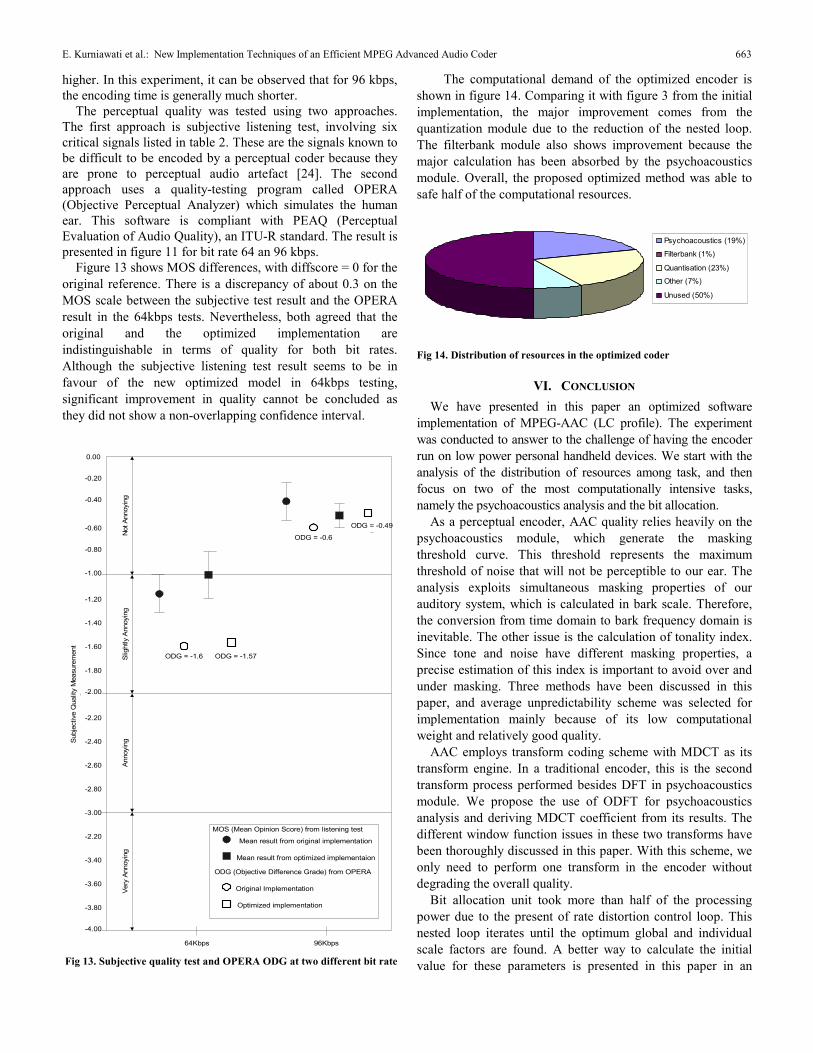
The perceptual quality was tested using two approaches. The first approach is subjective listening test, involving six critical signals listed in table 2. These are the signals known to be difficult to be encoded by a perceptual coder because they are prone to perceptual audio artefact [24]. The second approach uses a quality-testing program called OPERA (Objective Perceptual Analyzer) which simulates the human ear. This software is compliant with PEAQ (Perceptual Evaluation of Audio Quality), an ITU-R standard. The result is presented in figure 11 for bit rate 64 an 96 kbps. Figure 13 shows MOS differences, with diffscore = 0 for the original reference. There is a discrepancy of about 0.3 on the MOS scale between the subjective test result and the OPERA result in the 64kbps tests. Nevertheless, both agreed that the original and the optimized implementation are indistinguishable in terms of quality for both bit rates. Although the subjective listening test result seems to be in favour of the new optimized model in 64kbps testing, significant improvement in quality cannot be concluded as they did not show a non-overlapping confidence interval.

Not

Ann

oyin

gS

light

ly A

nnoy

ing

Ann

oyin

gV

ery

Ann

oyin

g

0.00

-1.00

-2.00

-3.00

-4.00

-0.20

-0.40

-0.60

-0.80

-1.20

-1.40

-1.60

-1.80

-2.20

-2.40

-2.60

-2.80

-2.20

-3.40

-3.60

-3.80

Sub

ject

ive

Qua

lity

Mea

sure

men

t

64Kbps 96Kbps

ODG = -1.6 ODG = -1.57

ODG = -0.6

ODG = -0.49

MOS (Mean Opinion Score) from listening test

ODG (Objective Difference Grade) from OPERA

Original Implementation

Optimized implementation

Mean result from original implementation

Mean result from optimized implementaion

Fig 13. Subjective quality test and OPERA ODG at two different bit rate

The computational demand of the optimized encoder is shown in figure 14. Comparing it with figure 3 from the initial implementation, the major improvement comes from the quantization module due to the reduction of the nested loop. The filterbank module also shows improvement because the major calculation has been absorbed by the psychoacoustics module. Overall, the proposed optimized method was able to safe half of the computational resources.

Psychoacoustics (19%)

Filterbank (1%)

Quantisation (23%)

Other (7%)

Unused (50%)

Fig 14. Distribution of resources in the optimized coder

VI. CONCLUSION We have presented in this paper an optimized software

implementation of MPEG-AAC (LC profile). The experiment was conducted to answer to the challenge of having the encoder run on low power personal handheld devices. We start with the analysis of the distribution of resources among task, and then focus on two of the most computationally intensive tasks, namely the psychoacoustics analysis and the bit allocation.

As a perceptual encoder, AAC quality relies heavily on the psychoacoustics module, which generate the masking threshold curve. This threshold represents the maximum threshold of noise that will not be perceptible to our ear. The analysis exploits simultaneous masking properties of our auditory system, which is calculated in bark scale. Therefore, the conversion from time domain to bark frequency domain is inevitable. The other issue is the calculation of tonality index. Since tone and noise have different masking properties, a precise estimation of this index is important to avoid over and under masking. Three methods have been discussed in this paper, and average unpredictability scheme was selected for implementation mainly because of its low computational weight and relatively good quality.

AAC employs transform coding scheme with MDCT as its transform engine. In a traditional encoder, this is the second transform process performed besides DFT in psychoacoustics module. We propose the use of ODFT for psychoacoustics analysis and deriving MDCT coefficient from its results. The different window function issues in these two transforms have been thoroughly discussed in this paper. With this scheme, we only need to perform one transform in the encoder without degrading the overall quality.

Bit allocation unit took more than half of the processing power due to the present of rate distortion control loop. This nested loop iterates until the optimum global and individual scale factors are found. A better way to calculate the initial value for these parameters is presented in this paper in an

IEEE Transactions on Consumer Electronics, Vol. 50, No. 2, MAY 2004

effort to avoid unnecessary iteration. The calculation of quantization error is improved using an estimator derived from the scale factor values. This saves us from performing the dequantization process in the encoder, as normally used in analysis by synthesis method to calculate the error.

The perceptual quality of the optimized encoder was evaluated using subjective listening test and objective evaluation of a quality testing program called OPERA. Both results show no significant degradation in the optimized coder for bit rate of 64kbps and 96 kbps, as overlapping confidence interval was obtained from both listening test.

The latest effort to further reduce the audio bit rate results in the standardization of High Efficiency – AAC (HE-AAC) as part of MPEG 4 systems, promising CD quality at 48 kbps. HE-AAC contains a standard AAC to code the low frequency region and a new Spectral Band Replication (SBR) technology to generate the high frequency portion. All the modifications highlighted in this paper can be utilized in the core coder of HE-AAC. Our future research will focus on the optimization of the SBR part of this newly defined coding system.

REFERENCES [1] ISO/IEC 14496-3, “Information Technology – Coding of audio-visual

objects, Part 3: Audio” (1999) [2] E.Kurniawati, J.Absar, S.George, C.T.Lau, B.Premkumar, “An

Investigation Into Different Masking Behaviours Resulting from Estimation of Tonality Index”, 14th International Conference on Digital Signal Processing, July 2002, Santorini, Greece.

[3] J.D. Johnston, “Estimation of Perceptual Entropy Using Noise Masking Criteria”, IEEE CH2561-9/88/0000-2524, 1988.

[4] J.D. Johnston, “Transform Coding of Audio Signals Using Perceptual Noise Criteria”, IEEE Journal on Selected Areas in Communications Vol.6No. 2, February 1988

[5] E.Kurniawati, J.Absar, S.George, C.T.Lau, B.Premkumar, “The Significance of Tonality Index and Nonlinear Psychoacoustics Models for Masking Threshold Estimation”, Audio Engineering Society 22nd International Conference on Virtual, Synthetic and Entertainment Audio, June 2002, Espoo, Finland.

[6] Ivan Dimkovic, Dragorad Milovanovic, Zoran Bojkovic, “Fast Software Implementation of MPEG Audio Encoder”, 14th International Conference on Digital Signal Processing, July 2002, Santorini, Greece.

[7] Toshiyuki Nomura, Yuchiro Takamizawa, “Processor-Efficient Implementation of a Hight Quality MPEG-2 AAC Encoder”, Audio Engineering Society 110th Convention 2001, Preprint #5294

[8] T.H. Tsai, S.W. Huang, L.G.Chen, “Design of a Low Power Psychoacoustic Model Co-Processor for MPEG-2/4 AAD LC Stereo Encoder”, 0-7803-7761-3/03, IEEE

[9] Yuichiro Takamizawa, Toshiyuki Nomura, and Masao Ikekawa, “High-Quality and Processor-Efficient Implementation of an MPEG-2 AAC Encoder”, 0-7803-7041-4/01, IEEE.

[10] A.D.Duenas, R. Perez, B.Rivas, E.Alexandre, A.S.Pena, “A robust and Efficient Implementation of MPEG-2/4 AAC Natural Audio Coders”, Audio Engineering Society 112th Convention 2002, Preprint #5556

[11] Ye Wang, Leonid Yaroslavsky, Miikka Vilermo, Mauri Vaananen, “Some Peculiar Properties of the MDCT”, 0-7803-5747-7/00, 2000.

[12] Anibal J.S. Ferreira, “Perceptual coding using sinusoidal modeling in the MDCT domain”, Audio Engineering Society 112th Convention 2002, Preprint #5569.

[13] E.Kurniawati, J.Absar, S.George, C.T.Lau, B.Premkumar, “Single Transform Perceptual Audio Encoder”,14th International Conference on Digital Signal Processing, July 2002, Santorini, Greece.

[14] Kai-Tat Fung, Yui-Lam Chan, Wan-Chi Siu, “A Fast Bit Allocation Algorithm for MPEG Audio Encoder”, Proceedings of 2001 International Symposium on Intelligent Multimedia, Video and Speech Processing, May 2001

[15] C.M. Liu, W.J. Lee, R.S. Hong, “Bit Allocation for Advanced Audio Coding using Bandwidth Proportional Noise Shaping Criterion”, Proceedings of the 6th International Conference on Digital Audio Effects (DAFX-03).

[16] Hyen-O Oh, Joon-Seok Kim, Chang-Jun Song, Young-Cheol Park, Dae Hee Youn, “Low Power MPEG/Audio Encoders Using Simplified Psychoacoustic model and Fast Bit Allocation”, 0-7803-6622-0/01, 2001 IEEE.

[17] Hyen-O Oh, Joon-Seok Kim, Chang-Jun Song, Dae-Hee Youn, Il-WhanCha, “New Implementation Techniques of A Real Time MPEG-2 Audio Encoding System”, 0-7803-5041-3/99, 1999 IEEE.

[18] A.D.Duenas, R. Perez, B.Rivas, E.Alexandre, A.S.Pena, “Realtime Implementation of MPEG-2 and MPET-4 Natural Audio Coders”, Audio Engineering Society 110th Convention 2001, Preprint #5302

[19] Manoj Kumar, Mohammad Zubair, “A High Performance Software Implementation of MPEG Audio Encoder”, ICASSP, Vol. 2, 1996

[20] C.M. Liu, W.J. Lee, R.S. Hong, “A New Crieterion and Associated Bit Allocation Method For Current Audio Coding Standards”, Proceedings of the 5th International Conference on Digital Audio Effects (DAFX-02).

[21] Chi-Min Liu, Chin-Ching Chen, Wen-Chieh Lee, Szu-Wei Lee, “A Fast Bit Allocation Method for MPEG Layer III”, 0-7803-5123-1/99, 1999 IEEE.

[22] C.Y.Lee, Y.C.Fang, H.C.Chuang, C.N.Wang, T.H. Chiang, “A Fast Audio Bit Allocation Technique Based on a Linear R-D Model”, IEEE Transactions of Consumer Electronics, Vol. 48, No.3, August 2002

[23] Kelvin H.C. Eng, D.Y.Huang, S.W. Foo, “A New Bit Allocation Method for Low Delay Audio Coding at Low Bit Rates”, Audio Engineering Society 112th Convention 2002, Preprint #5573

[24] Markus Erne, “Perceptual Audio Coders, What to listen for”, Audio Engineering Society 111th Convention 2001

Evelyn Kurniawati received her Bachelor of Applied Science (Computer Engineering) degree from Nanyang Technological Uniersity (NTU) Singapore in 2000. She is now pursuing her doctoral degree in School of Computer Engineering, NTU. Her research interest are in digital audio compression, network security and computer animation. Chiew-Tong Lau received his B.Eng. degree from Lakehead University in 1983, and M.A.Sc and Ph.D. degrees in Electrical Engineering from the University of British Columbia in 1985 and 1990 respectively. He is currently an Associate Professor and Head of Division of Computer Communications in the School of Computer Engineering, Nanyang Technological University, Singapore. His main research interests are in

wireless communications.

Benjamin Premkumar received his Bachelor of Science degree in Physics and Math from Bangalore University (India) and a Bachelor’s degree in Electrical communication Engineering from the Indian Institute of Science (India). He briefly worked in large communication industry in Bangalore in their Research and Development division before proceeding to the US to earn his M.S. from North Dakota State University.

His MS research was in the area of Digital Speech Processing. He taught as a graduate teaching fellow at NDSU. He then went on to obtain his PhD from University of Idaho. His PhD thesis was in the area of Synthetic Aperture Radar Signal Processing, a project funded by NASA.

He has held various teaching positions since 1991 both in the US and Singapore. Currently he is an Associate Professor in the school of Computer Engineering (NTU). His research interests include Digital Signal Processing and its applications in Wireless Communication, Software Defined Radio and Impulse Radio. He also works in the area of multirate signal processing, filter banks, transform techniques, speech coding techniques, Number Theory, Wavelet transform and its application to signal analysis.

664

E. Kurniawati et al.: New Implementation Techniques of an Efficient MPEG Advanced Audio Coder 665

Javed Absar received his Bachelor of Applied Science (Computer Engineering) degree from Nanyang Technological University (NTU) Singapore in 1996. He has been with ST Microelectronics Asia Pacific Pte. Ltd. since then, working on audio compression scheme and low power compiler. His main research interests are in low power design for multimedia. Sapna George completed her BTech in Electronics and Communications in 1985 from College of Engineering, Kerala, India. Since 1995, she has been with ST Microelectronics Asia Pacific Pte. Ltd. She is Technical Manager, in charge of Audio research and development at STMicroelectronics's R&D centre in Singapore.