New Geometric Techniques for Linear Programming and Graph Partitioning by Jonathan A. Kelner Submitted to the Department of Electrical Engineering and Computer Science in partial fulfillment of the requirements for the degree of Doctor of Philosophy at the MASSACHUSETTS INSTITUTE OF TECHNOLOGY September 2006 c Jonathan A. Kelner, MMVI. All rights reserved. The author hereby grants to MIT permission to reproduce and distribute publicly paper and electronic copies of this thesis document in whole or in part. Author .............................................................. Department of Electrical Engineering and Computer Science August 15, 2006 Certified by .......................................................... Daniel A. Spielman Professor of Applied Mathematics and Computer Science, Yale University Thesis Co-Supervisor Certified by .......................................................... Madhu Sudan Professor of Computer Science Thesis Co-Supervisor Accepted by ......................................................... Arthur C. Smith Chairman, Committee for Graduate Students

Welcome message from author
This document is posted to help you gain knowledge. Please leave a comment to let me know what you think about it! Share it to your friends and learn new things together.
Transcript

New Geometric Techniques for Linear
Programming and Graph Partitioning
by
Jonathan A. Kelner
Submitted to the Department of Electrical Engineering and ComputerScience
in partial fulfillment of the requirements for the degree of
Doctor of Philosophy
at the
MASSACHUSETTS INSTITUTE OF TECHNOLOGY
September 2006
c© Jonathan A. Kelner, MMVI. All rights reserved.
The author hereby grants to MIT permission to reproduce anddistribute publicly paper and electronic copies of this thesis document
in whole or in part.
Author . . . . . . . . . . . . . . . . . . . . . . . . . . . . . . . . . . . . . . . . . . . . . . . . . . . . . . . . . . . . . .Department of Electrical Engineering and Computer Science
August 15, 2006
Certified by. . . . . . . . . . . . . . . . . . . . . . . . . . . . . . . . . . . . . . . . . . . . . . . . . . . . . . . . . .Daniel A. Spielman
Professor of Applied Mathematics and Computer Science, YaleUniversity
Thesis Co-Supervisor
Certified by. . . . . . . . . . . . . . . . . . . . . . . . . . . . . . . . . . . . . . . . . . . . . . . . . . . . . . . . . .Madhu Sudan
Professor of Computer ScienceThesis Co-Supervisor
Accepted by . . . . . . . . . . . . . . . . . . . . . . . . . . . . . . . . . . . . . . . . . . . . . . . . . . . . . . . . .Arthur C. Smith
Chairman, Committee for Graduate Students
New Geometric Techniques for Linear Programming and
Graph Partitioning
byJonathan A. Kelner
Submitted to the Department of Electrical Engineering and Computer Scienceon August 15, 2006, in partial fulfillment of the
requirements for the degree ofDoctor of Philosophy
Abstract
In this thesis, we advance a collection of new geometric techniques for the analysisof combinatorial algorithms. Using these techniques, we resolve several longstandingquestions in the theory of linear programming, polytope theory, spectral graph theory,and graph partitioning.
The thesis consists of two main parts. In the first part, which is joint work withDaniel Spielman, we present the first randomized polynomial-time simplex algorithmfor linear programming, answering a question that has been open for over fifty years.Like the other known polynomial-time algorithms for linear programming, its runningtime depends polynomially on the number of bits used to represent its input.
To do this, we begin by reducing the input linear program to a special form inwhich we merely need to certify boundedness of the linear program. As boundednessdoes not depend upon the right-hand-side vector, we run a modified version of theshadow-vertex simplex method in which we start with a random right-hand-side vectorand then modify this vector during the course of the algorithm. This allows us toavoid bounding the diameter of the original polytope.
Our analysis rests on a geometric statement of independent interest: given apolytope x |Ax ≤ b in isotropic position, if one makes a polynomially small per-turbation to b then the number of edges of the projection of the perturbed polytopeonto a random 2-dimensional subspace is expected to be polynomial.
In the second part of the thesis, we address two long-open questions about findinggood separators in graphs of bounded genus and degree:
1. It is a classical result of Gilbert, Hutchinson, and Tarjan [25] that one can findasymptotically optimal separators on these graphs if he is given both the graphand an embedding of it onto a low genus surface. Does there exist a simple,efficient algorithm to find these separators given only the graph and not theembedding?
2. In practice, spectral partitioning heuristics work extremely well on these graphs.Is there a theoretical reason why this should be the case?
2
We resolve these two questions by showing that a simple spectral algorithm findsseparators of cut ratio O(
√g/n) and vertex bisectors of size O(
√gn) in these graphs,
both of which are optimal. As our main technical lemma, we prove an O(g/n) boundon the second smallest eigenvalue of the Laplacian of such graphs and show that thisis tight, thereby resolving a conjecture of Spielman and Teng. While this lemma isessentially combinatorial in nature, its proof comes from continuous mathematics,drawing on the theory of circle packings and the geometry of compact Riemannsurfaces.
While the questions addressed in the two parts of the thesis are quite different,we show that a common methodology runs through their solutions. We believe thatthis methodology provides a powerful approach to the analysis of algorithms that willprove useful in a variety of broader contexts.
Thesis Co-Supervisor: Daniel A. SpielmanTitle: Professor of Applied Mathematics and Computer Science, Yale University
Thesis Co-Supervisor: Madhu SudanTitle: Professor of Computer Science
3

Acknowledgments
First and foremost, I would like to thank Daniel Spielman for being a wonderfulmentor and friend. He has taught me a tremendous amount, not just about how tosolve problems, but about how to choose them. He helped me at essentially everystage of this thesis, and it certainly would not have been possible without him. I wastruly lucky to have him as my advisor, and I owe him a great debt of gratitude.
I would also like to thank:
Sophie, my family, and all of my friends for their continued love, support, and, ofcourse, tolerance of me throughout my graduate career;
Shang-Hua Teng for introducing me to the question addressed in the second part ofthis thesis and for several extremely helpful conversations about both spectralpartitioning and academic life;
All of the faculty and other students in the Theory group at MIT for providing anexciting and stimulating environment for the past four years;
Nathan Dunfield, Phil Bowers, and Ken Stephenson for their guidance on the theoryof circle packings
Christopher Mihelich for his help in simplifying the proof of Lemma /citeorthog toones and for sharing his uncanny knowledge of TeX;
The anonymous referees at the SIAM Journal on Computing for their very helpfulcomments and suggestions about the spectral partitioning portion of the thesis;
Microsoft Research for hosting me over the summer of 2004;
Madhu Sudan and Piotr Indyk for serving on my thesis committee and for severalvery helpful comments about how to improve this thesis.
4
Previous Publications of this Work
Much of the material in this thesis has appeared in previously published work. Inparticular, the material on the simplex method in the introduction and the contentsof chapters three through seven represent joint work with Daniel Spielman and werepresented at STOC 2006 [37]. The introductory material on spectral partitioning andchapters eight through twelve were presented at STOC 2004 [33] and were expandedupon in my Master’s thesis [34] and in the STOC 2004 Special Issue of the SIAMJournal on Computing [35]. In all of these cases, this thesis draws from the aboveworks without further mention.
5

Contents
Acknowledgements 4
Previous Publications of this Work 5
Table of Contents 6
List of Figures 8
1 Introduction 9
1.1 A Randomized Polynomial-Time Simplex Method for Linear Program-ming . . . . . . . . . . . . . . . . . . . . . . . . . . . . . . . . . . . . 9
1.2 Spectral Partitioning, Eigenvalue Bounds, and Circle Packings for Graphsof Bounded Genus . . . . . . . . . . . . . . . . . . . . . . . . . . . . 12
1.3 The Common Methodology . . . . . . . . . . . . . . . . . . . . . . . 13
I A Randomized Polynomial-Time Simplex Algorithm forLinear Programming 14
2 Introduction to Linear Programming Geometry 15
2.1 Linear Programs as Polytopes . . . . . . . . . . . . . . . . . . . . . . 152.2 Duality . . . . . . . . . . . . . . . . . . . . . . . . . . . . . . . . . . . 162.3 Polarity . . . . . . . . . . . . . . . . . . . . . . . . . . . . . . . . . . 192.4 When is a Linear Program Unbounded? . . . . . . . . . . . . . . . . 19
3 The Simplex Algorithm 21
3.1 The General Method . . . . . . . . . . . . . . . . . . . . . . . . . . . 213.2 The Shadow-Vertex Method . . . . . . . . . . . . . . . . . . . . . . . 22
4 Bounding the Shadow Size 23
4.1 The Shadow Size in the k-Round Case . . . . . . . . . . . . . . . . . 234.2 The Shadow Size in the General Case . . . . . . . . . . . . . . . . . . 30
6
5 Reduction of Linear Programming to Certifying Boundedness 34
5.1 Reduction to a Feasibility Problem . . . . . . . . . . . . . . . . . . . 345.2 Degeneracy and the Reduction to Certifying Boundedness . . . . . . 37
6 Our Algorithm 41
6.1 Constructing a Starting Vertex . . . . . . . . . . . . . . . . . . . . . 426.2 Polytopes that are not k-Round . . . . . . . . . . . . . . . . . . . . . 436.3 Towards a Strongly Polynomial-Time Algorithm for Linear Program-
ming? . . . . . . . . . . . . . . . . . . . . . . . . . . . . . . . . . . . 47
7 Geometric Lemmas for Algorithm’s Correctness 48
7.1 2-Dimensional Geometry Lemma . . . . . . . . . . . . . . . . . . . . 497.2 High-Dimensional Geometry Lemma . . . . . . . . . . . . . . . . . . 50
II Spectral Partitioning, Eigenvalue Bounds, and CirclePackings for Graphs of Bounded Genus 52
8 Background in Graph Theory and Spectral Partitioning 53
8.1 Graph Theory Definitions . . . . . . . . . . . . . . . . . . . . . . . . 538.2 Spectral Partitioning . . . . . . . . . . . . . . . . . . . . . . . . . . . 54
9 Outline of the Proof of the Main Technical Result 56
10 Introduction to Circle Packings 58
10.1 Planar Circle Packings . . . . . . . . . . . . . . . . . . . . . . . . . . 5810.2 A Very Brief Introduction to Riemann Surface Theory . . . . . . . . 6010.3 Circle Packings on Surfaces of Arbitrary Genus . . . . . . . . . . . . 62
11 An Eigenvalue Bound 64
12 The Proof of the Subdivision Lemma 70
Bibliography 79
7
List of Figures
4-1 The points x, y and q. . . . . . . . . . . . . . . . . . . . . . . . . . . 28
7-1 The geometric objects considered in Lemma 7.1.1 . . . . . . . . . . . 49
8-1 The surfaces of genus 0, 1, 2, and 3. . . . . . . . . . . . . . . . . . . 54
10-1 A univalent circle packing with its associated graph. . . . . . . . . . 5910-2 A nonunivalent circle packing with its associated graph. . . . . . . . . 59
11-1 The hexagonal subdivision procedure applied to a triangulation withtwo triangles. . . . . . . . . . . . . . . . . . . . . . . . . . . . . . . . 66
12-1 A subdivided graph, with P (w) and N(w) shaded for a vertex w. . . 7312-2 An illustration of how the grid graph exists as a subgraph of the union
of two adjacent subdivided triangles. . . . . . . . . . . . . . . . . . . 7412-3 The entire construction illustrated for a given edge of the original graph. 75
8
Chapter 1
Introduction
In this thesis, we advance a collection of new geometric techniques for the analysisof combinatorial algorithms. Using these techniques, we resolve several longstandingquestions in the theory of linear programming, polytope theory, spectral graph theory,and graph partitioning.
In this chapter, we shall introduce and summarize the main contributions of thisthesis. The remainder of this document will be divided into two main parts. Here,we discuss the main components of each part and then briefly explain the commonmethodology that runs between the two. The contents of this thesis are drawn heavilyfrom previously published works; please see page 5 for a full discussion of the originsof the different sections.
1.1 A Randomized Polynomial-Time Simplex
Method for Linear Programming
In the first part of this thesis, we shall present the first randomized polynomial-timesimplex method for linear programming. Linear programming is one of the funda-mental problems of optimization. Since Dantzig [14] introduced the simplex methodfor solving linear programs, linear programming has been applied in a diverse rangeof fields including economics, operations research, and combinatorial optimization.From a theoretical standpoint, the study of linear programming has motivated majoradvances in the study of polytopes, convex geometry, combinatorics, and complexitytheory.
While the simplex method was the first practically useful approach to solvinglinear programs and is still one of the most popular, it was unknown whether anyvariant of the simplex method could be shown to run in polynomial time in the worstcase. In fact, most common variants have been shown to have exponential worst-case
9

CHAPTER 1. INTRODUCTION 10
complexity. In contrast, algorithms have been developed for solving linear programsthat do have polynomial worst-case complexity [38, 32, 19, 4]. Most notable amongthese have been the ellipsoid method [38] and various interior-point methods [32]. Allprevious polynomial-time algorithms for linear programming of which we are awarediffer from simplex methods in that they are fundamentally geometric algorithms:they work either by moving points inside the feasible set, or by enclosing the feasibleset in an ellipse. Simplex methods, on the other hand, walk along the vertices andedges defined by the constraints. The question of whether such an algorithm can bedesigned to run in polynomial time has been open for over fifty years.
We recall that a linear program is a constrained optimization problem of the form:
maximize c · x (1.1)
subject to Ax ≤ b, x ∈ Rd,
where c ∈ Rd and b ∈ Rn are column vectors, and A is an n×d matrix. The vector c
is the objective function, and the set P := x | Ax ≤ b is the set of feasible points.If it is non-empty, P is a convex polyhedron, and each of its extreme vertices will bedetermined by d constraints of the form aaai · x = bi, where aaa1, . . . ,aaan are the rowsof A. It is not difficult to show that the objective function is always maximized at anextreme vertex, if this maximum is finite.
The first simplex methods used heuristics to guide a walk on the graph of verticesand edges of P in search of one that maximizes the objective function. In orderto show that any such method runs in worst-case polynomial time, one must provea polynomial upper bound on the diameter of polytope graphs. Unfortunately, theexistence of such a bound is a wide-open question: the famous Hirsch Conjectureasserts that the graph of vertices and edges of P has diameter at most n−d, whereasthe best known bound for this diameter is superpolynomial in n and d [31].
Later simplex methods, such as the self-dual simplex method and the criss-crossmethod [15, 22], tried to avoid this obstacle by considering more general graphsfor which better diameter bounds were possible. However, even though some ofthese graphs have polynomial diameters, they have exponentially many vertices, andnobody had been able to design a polynomial-time algorithm that provably finds theoptimum after following a polynomial number of edges. In fact, essentially every suchdeterministic algorithm has well-known counterexamples on which the walk takesexponentially many steps. However, for randomized pivot rules very little is known.While the best previously known upper bounds on the running time of randomizedpivot rule is Ω
(exp
(√d log n
))[30], there exist very simple randomized pivots rules
for which essentially no nontrivial lower bounds have been shown.In this thesis, we present the first randomized polynomial-time simplex method.
Like the other known polynomial-time algorithms for linear programming, the running
CHAPTER 1. INTRODUCTION 11
time of our algorithm depends polynomially on the bit-length of the input. We donot prove an upper bound on the diameter of polytopes. Rather we reduce thelinear programming problem to the problem of determining whether a set of linearconstraints defines an unbounded polyhedron. We then randomly perturb the right-hand sides of these constraints, observing that this does not change the answer, andwe then use a shadow-vertex simplex method to try solve the perturbed problem.When the shadow-vertex method fails, it suggests a way to alter the distributions ofthe perturbations, after which we apply the method again. We prove that the numberof iterations of this loop is polynomial with high probability.
It is important to note that the vertices considered during the course of the al-gorithm may not all appear on a single polytope. Rather, they may be viewed asappearing on the convex hulls of polytopes with different b-vectors. It is well-knownthat the graph of all of these “potential” vertices has small diameter. However, therewas previously no way to guide a walk among these potential vertices to one opti-mizing any particular objective function. Our algorithm uses the graphs of polytopes“near” P to impose structure on this graph and to help to guide our walk.
Perhaps the message to take away from this is that instead of worrying aboutthe combinatorics of the natural polytope P , one can reduce the linear programmingproblem to one whose polytope is more tractable. The first result of this part of thethesis, and the inspiration for the algorithm, captures this idea by showing that if oneslightly perturbs the b-vector of a polytope in near-isotropic position, then there willbe a polynomial-step path from the vertex minimizing to the vertex maximizing arandom objective function. Moreover, this path may be found by the shadow-vertexsimplex method.
We stress that while our algorithm involves a perturbation, it is intrinsically dif-ferent from previous papers that have provided average-case or smoothed analyses oflinear programming. In those papers, one shows that, given some linear program, onecan probably use the simplex method to solve a nearby but different linear program;the perturbation actually modified the input. In the present document, our perturba-tion is used to inform the walk that we take on the (feasible or infeasible) vertices ofour linear program; however, we actually solve the exact instance that we are given.We believe that ours is the first simplex algorithm to achieve this, and we hope thatour results will be a useful step on the path to a strongly polynomial-time algorithmfor linear programming.
CHAPTER 1. INTRODUCTION 12
1.2 Spectral Partitioning, Eigenvalue Bounds, and
Circle Packings for Graphs of Bounded Genus
In the second part of the thesis, we shall take up several long-open problems in thespectral and algorithmic theory of graphs. Spectral methods have long been usedas a heuristic in graph partitioning. They have had tremendous experimental andpractical success in a wide variety of scientific and numerical applications, includingmapping finite element calculations on parallel machines [46, 51], solving sparse linearsystems [9, 10], partitioning for domain decomposition, and VLSI circuit design andsimulation [8, 28, 2]. However, it is only recently that people have begun to supplyformal justification for their efficacy [27, 47]. In [47], Spielman and Teng used theresults of Mihail [41] to show that the quality of the partition produced by the ap-plication of a certain spectral algorithm to a graph can be established by proving anupper bound on the Fiedler value of the graph (i.e., the second smallest eigenvalue ofits Laplacian). They then provided an O(1/n) bound on the Fielder value of a pla-nar graph with n vertices and bounded maximum degree. This showed that spectralmethods can produce a cut of ratio O(
√1/n) and a vertex bisector of size O(
√n) in
a bounded degree planar graph.In this part of the thesis, we use the theory of circle packings and conformal
mappings of compact Riemann surfaces to generalize these results to graphs of positivegenus. We prove that the Fiedler value of a genus g graph of bounded degree is O(g/n)and demonstrate that this is asymptotically tight, thereby resolving a conjecture ofSpielman and Teng. We then apply this result to obtain a spectral partitioningalgorithm that finds separators whose cut ratios are O(
√g/n) and vertex bisectors
of size O(√
gn), both of which are optimal. To our knowledge, this provides the onlytruly practical algorithm for finding such separators and vertex bisectors for graphsof bounded genus and degree. While there exist other asymptotically fast algorithmsfor this, they all rely on being given an embedding of the graph in a genus g surface(e.g., [25]). It is not always the case that we are given such an embedding, andcomputing it is quite difficult. (In particular, computing the genus of a graph isNP-hard [49], and the best known algorithms for constructing such an embeddingare either nO(g) [20] or polynomial in n but doubly exponential in g [17]. Mohar hasfound an algorithm that depends only linearly on n [42], but it has an uncalculatedand very large dependence on g.) The excluded minor algorithm of Alon, Seymour,and Thomas [1] does not require an embedding of the graph, but the separators thatit produces are not asymptotically optimal.
The question of whether there exists an efficient algorithm for providing asymp-totically optimal cuts without such an embedding was first posed twenty years ago

CHAPTER 1. INTRODUCTION 13
by Gilbert, Hutchinson, and Tarjan [25].1 We resolve this question here, as our algo-rithm proceeds without any knowledge of an embedding of the graph, and it insteadrelies only on simple matrix manipulations of the adjacency matrix of the graph.While the analysis of the algorithm requires some somewhat involved mathematics,the algorithm itself is quite simple, and it can be implemented in just a few linesof Matlab code. In fact, it is only a slight modification of the spectral heuristicsfor graph partitioning that are widely deployed in practice without any theoreticalguarantees.
We believe that the techniques that we employ to obtain our eigenvalue boundsare of independent interest. To prove these bounds, we make what is perhaps thefirst real use of the theory of circle packings and conformal mappings of positivegenus Riemann surfaces in the computer science literature. This is a powerful theory,and we believe that it will be useful for addressing other questions in spectral andtopological graph theory.
1.3 The Common Methodology
While the results proven in the two parts of the thesis are quite different, it willbecome clear that a common methodology that runs between them. In both cases,we provide bounds on the performance of algorithms using very similar geometrictechniques. In particular, the innovations of this thesis revolve around new techniquesfor relating the performance of combinatorial algorithms to geometric quantities andthen using a careful volumetric analysis to bound these quantities. To do so, weintroduce a variety of tools from pure mathematics that are not typically used in acomputer science context, including Riemann surface theory, differential and algebraicgeometry, circle packing theory, geometric probability theory, harmonic analysis, andconvex geometry.
The techniques advanced herein appear to be quite widely applicable and havealready been applied in a variety of broader contexts [36, 43]. In one noteworthy suchapplication, Kelner and Nikolova use random matrix theory to generalize the analysisof the simplex method to provide the first smoothed polynomial-time algorithm fora broad class on nonconvex optimization problems [36], providing an illustration ofthe wide-ranging usefulness of the ideas that we shall present.
1Djidjev claimed in a brief note to have such an algorithm [18], but it has never appeared in theliterature.

Part I
A Randomized Polynomial-Time
Simplex Algorithm for Linear
Programming
14

Chapter 2
Introduction to Linear
Programming Geometry
In this section, we shall briefly review some basic facts about linear programminggeometry and the simplex method. As this material is quite standard, we shall oftenomit the proofs and aim only for intuition. For a more thorough treatment of theclassical theory of linear programming, see Chvatal’s book [13], or see Vanderbei’sbook [50] for a more modern viewpoint.
2.1 Linear Programs as Polytopes
Suppose that we are given a linear program of the form described in equation (1.1):
maximize c · xsubject to Ax ≤ b, x ∈ Rd,
where c ∈ Rd and b ∈ Rn are column vectors and A is an n × d matrix, and let
P = x ∈ Rd |Ax ≤ b
be its feasible region. Suppose further that the feasible region is nonempty and hasnonempty interior. In particular, this implies that P is full-dimensional and thereforeis not contained in any proper linear subspace of Rd. 1 If aaa1, . . . ,aaan are the rows of
1We make these assumptions solely to facilitate the exposition in this section; our actual algorithmwill work for fully general linear programs.
15
CHAPTER 2. INTRODUCTION TO LP GEOMETRY 16
A, then we can rewrite the feasible region as
P = x ∈ Rd |aaai · x ≤ bi, ∀i =
n⋂
i=1
Hi,
whereHi = x ∈ R
d |aaai · x ≤ bi, ∀i.We now note a sequence of simple facts that will provide us with a dictionary to
translate the given algebraic formulation of our linear program into a geometric one:
• Each of the Hi is a half-space, and their intersection P is a convex polyhedron2.
• Each facet of P may be given as the set of points at which some constraintaaai · x ≤ bi is tight (i.e., where it is satisfied with equality).
• Each face of codimension k may be given as the set of points at which somecollection of k constraints is tight. In particular, every vertex is the point atwhich a collection of d constaints is tight.
• If P is bounded, the objective function will have a finite maximum.
• Since the objective function is linear and P is convex, every local maximum isa global maximum as well.
• If the objective function has a finite maximum, all points at which it is maxi-mized occur on the boundary of P . The collection of such points constitutes aproper face of P and, in particular, contains some vertex of P .
Remark 2.1.1. The last fact implies that it suffices to search over the vertices of Pto find the optimum. We shall make significant use of this in Chapter 3 when weintroduce the simplex method.
2.2 Duality
In this section, we shall introduce one of the basic tools for linear programming:duality. Given any linear program, linear programming duality allows us to constructa second linear program (in a slightly modified form) that appears quite differentfrom the original but actually has the same optimal value.
2From here on, all polyhedra shall be assumed convex, unless otherwise noted.

CHAPTER 2. INTRODUCTION TO LP GEOMETRY 17
Definition 2.2.1. Let P be the linear program
maximize c · xsubject to Ax ≤ b, x ∈ Rd
Its dual is the linear program D given by
minimize b · ysubject to ATy = c, y ≥ 0 .
We shall call the original linear program the primal linear program when we wish tocontrast it with the dual.
Theorem 2.2.2 (Strong Linear Programming Duality). The primal and dual linearprograms have the same optimal value. That is, if either the primal or dual programis feasible with a finite optimum, then both are feasible with finite optima. In thiscase, if x 0 is the point that maximizes c ·x in the primal program and y 0 is the pointthat minimizes b · y in the dual program, then c · x 0 = b · y 0.
Lemma 2.2.3 (Weak Linear Programming Duality). For any x 0 that is feasible forP and any y 0 that is feasible for D,
c · x 0 ≤ b · y 0.
In particular, this inequality holds for x 0 and y0 as described in the statement ofTheorem 2.2.2.
Proof of Lemma 2.2.3. Since x 0 is feasible for P, we have that Ax 0 ≤ b. Any y 0
that is feasible for D has all positive components, so multiplying this inequality onthe left by yT
0 yieldsyT
0 Ax 0 ≤ yT0 b. (2.1)
However, the feasibility of y 0 implies that yT0 A = cT . Combining this with equa-
tion 2.1 yieldscTx 0 = yT
0 Ax 0 ≤ yT0 b,
as desired.
We now use weak duality to sketch a proof of strong duality. The argument usedhere is a slightly nonstandard one; it is drawn from Schrijver’s book on linear andinteger programming [45].
CHAPTER 2. INTRODUCTION TO LP GEOMETRY 18
Sketch of Proof of Theorem 2.2.2. Let the polyhedron P be the feasible region of P.We assume here that P is nonempty and bounded. The other cases inhere no signif-icant additional difficulties and are omitted for concision.
Our proof sketch is based on Newtonian physics3. We place a ball inside of ourpolyhedron P , and we subject this ball to a “gravitational” force with the samemagnitude and direction as c. We then let the ball roll down to its resting place,which will be the point x 0 that maximizes the dot product c ·x 0, and we analyze theforces on the ball at equilibrium.
In order for the ball to be at rest, the total force on the ball must equal zero.Facets may only exert forces in their normal directions, and the forces may only bedirected inward. As such, the ith facet may only exert a force f i in the direction ofaaai, and this force must have a negative dot product with aaai. We can thus define avector y0 with all positive components such that f i = −y0iaaai for all i.
Since the total force on the ball must equal zero, we have
0 T = cT +∑
i
f i = cT −∑
i
y0iaaai = cT − yT0 A,
and thusATy0 = c.
It therefore follows that y 0 is feasible for D.Now, the only facets that can exert a nonzero force on the ball are the ones that
are touching it, i.e., those i for which aaa i ·x 0 = bi. This is equivalent to the statementthat
(aaai · x 0 − bi)yi = 0 for all i,
or, written in matrix form,yT
0 (Ax 0 − b) = 0 .
It thus follows that we have a point x 0 that is feasible for P and a point y 0 that isfeasible for D for which
cTx 0 = yT0 Ax 0 = yT
0 b.
This implies that the maximum value of c · x in P is greater than or equal to theminimum value of b · y in D. Weak duality implies the opposite inequality, and thedesired theorem follows.
Remark 2.2.4. By weak linear programming duality, every feasible point of the dual
3This recourse to physics is not fully rigorous and leaves us with something between an intuitionand a proof. Nevertheless, our intuition may easily be translated into a rigorous argument; seeSchrijver’s book [45] for the details.
CHAPTER 2. INTRODUCTION TO LP GEOMETRY 19
program yields a finite upper bound on the maximum of the primal program, andevery feasible point of the primal program yields a finite lower bound on the minimumof the dual program. Furthermore, the argument used in the proof of strong dualityshows that a finite optimum for one program yields a feasible point for the other. Itthus follows that P is bounded if and only if D is feasible, and D is bounded if andonly if P is feasible.
2.3 Polarity
In this section, we shall consider another type of duality operation known as polarity,which operates on convex polyhedra, not linear programs. While it is sometimesreferred to as polyhedron duality, we stress that polarity bears no relation to linearprogramming duality and is a completely different operation.
Polarity may actually be defined on the larger class of arbitrary convex bodies, butfor our purposes it will suffice to restrict our attention to polyhedra containing theorigin in their interiors. Any such polyhedron can be described as x ∈ Rd |aaai · x ≤bi, i = 1, . . . , n where all of the bi are strictly positive and the aaai span Rd. For anexposition of the general theory, see the book by Bonneson and Fenchel /citeBF.
Definition 2.3.1. Let P = x ∈ Rd |aaai · x ≤ bi, i = 1, . . . , n be a polyhedron withbi > 0 for all i. Its polar P ∗ is the polyhedron given by the convex hull
P ∗ = conv(aaa1/b1, . . . ,aaan/bn).
2.4 When is a Linear Program Unbounded?
Suppose that we are given a linear program with feasible region P = x ∈ Rd |Ax ≤b with b > 0. In this section, we take up the question of when P is unbounded. Itturns out that there is a very simple criterion for this in terms of the polar polytopeP ∗.
Theorem 2.4.1. Let P be as above. P is unbounded if and only if there exists avector q ∈ Rd such that the polar polytope P ∗ is contained in the halfspace Hq =x ∈ Rd | q · x ≤ 0.
Proof. Suppose first that P is unbounded. Since P contains the origin and is convex,this implies that there exists some vector q for which the ray r q := tq | t ≥ 0extends off to infinity while remaining inside of P . We claim that this implies thatP ∗ ⊆ Hq .
CHAPTER 2. INTRODUCTION TO LP GEOMETRY 20
To see this, suppose to the contrary that P ∗ 6⊆ Hq . This implies that thereexists some aaai for which aaai/bi /∈ Hq , i.e., for which (aaai/bi) · q > 0. In this case,the corresponding inequality aaai · x ≤ bi will be violated by the point tq whenevert > bi/(aaai · q), contradicting the infinitude of the ray r q .
For the converse, we shall suppose that P is bounded and shall deduce that P ∗ isnot contained in any halfspace through the origin. Indeed, this follows from the sameargument as above: if P ∗ were contained in the halfspace Hq then the ray r q wouldextend off to infinity, which would contradict the presumed boundedness of P .
A convex body is contained in a half-space if and only if it does not contain theorigin in its interior. We thus deduce:
Corollary 2.4.2. P is bounded if and only if P ∗ contains the origin in its interior.
Remark 2.4.3. Corollary 2.4.2 allows us to produce a certificate of boundedness forP by expressing the origin as a convex combination of the aaai with all strictly positivecoefficients. (The positivity of the coefficients guarantees that the origin is containedin the interior and not on the boundary of P ∗. Here, we use our assumption that theaaai span Rd.) We shall make use of this in Chapters 5 and 6.
Chapter 3
The Simplex Algorithm
In this chapter, we shall introduce our primary object of study, the simplex algorithm.As this material is standard and widely available, we shall restrict our discussion toa high-level overview. For an implementation-level discussion of the simplex method,we refer the reader to Vanderbei’s book [50].
3.1 The General Method
As we saw in Section 2.1, the feasible region of a linear program is a polytope P , theobjective function achieves its maximum at a vertex of P , and the objective functionhas no nonglobal local maxima. It thus suffices to search among the vertices for alocal maximum of the objective function.
Since P has finitely many vertices, this suggests an obvious algorithm for linearprogramming, known as the simplex algorithm or simplex method. Simply neglect allof the higher-dimensional faces of P and just consider the graph of vertices and edgesof P . Start at some vertex and walk along the edges of the graph until you find avertex that is a local (and thus global) maximum.
Of course, the above is really just a meta-algorithm. To make it into a fullyspecified algorithm, one must further specify two things:
1. How does one obtain the starting vertex?
2. Given the current vertex, how does one obtain the next vertex? This is knownas the pivot rule.
Since the simplex method was first introduced, this definition has been broadened toallow the algorithm to walk on other graphs associated with the polytope; noteworthyexamples of such algorithms include the self-dual simplex method and the criss-cross
21
CHAPTER 3. THE SIMPLEX ALGORITHM 22
method [15, 22]. Nevertheless, while there have been numerous pivot rules set forthfor linear programming, up until the present work none have been shown to terminatein a polynomial number of steps.
In the following section, we shall describe a classical pivot rule known as the“shadow-vertex method.” We stress that this pivot rule does not always terminatein a polynomial number of steps. Instead, we shall use it as a component of a morecomplicated algorithm that does indeed have the desired polynomial running time.
3.2 The Shadow-Vertex Method
Let P be a convex polyhedron, and let S be a two-dimensional subspace. The shadowof P onto S is simply the projection of P onto S. The shadow is a polygon, and everyvertex (edge) of the polygon is the image of some vertex (edge) of P . One can showthat the set of vertices of P that project onto the boundary of the shadow polygonare exactly the vertices of P that optimize objective functions in S [6, 24].
These observations are the inspiration for the shadow-vertex simplex method,which lifts the simplicity of linear programming in two dimensions to the generalcase [6, 24]. To start, the shadow-vertex method requires as input a vertex v 0 of P .It then chooses some objective function optimized at v 0, say f , sets S = span(c, f ),and considers the shadow of P onto S. If no degeneracies occur, then for each vertexy of P that projects onto the boundary of the shadow, there is a unique neighbor ofy on P that projects onto the next vertex of the shadow in clockwise-order. Thus,by tracing the vertices of P that map to the boundary of the shadow, the shadow-vertex method can move from the vertex it knows that optimizes f to the vertex thatoptimizes c. The number of steps that the method takes will be bounded by thenumber of edges of the shadow polygon. For future reference, we call the shadow-vertex simplex method by
ShadowVertex(aaa1, . . . ,aaan, b, c, S, v0, s),
where aaa1, . . . ,aaan, b, and c specify a linear program of form (1.1), S is a two-dimensionalsubspace containing c, and v 0 is the start vertex, which must optimize some objectivefunction in S. We allow the method to run for at most s steps. If it has not foundthe vertex optimizing c within that time, it should return (fail, y), where y is itscurrent vertex. If it has solved the linear program, it either returns (opt, x ), wherex is the solution, or unbounded if it was unbounded.

Chapter 4
Bounding the Shadow Size
In this chapter, we shall show that if the polytope is in a “good” coordinate system andthe distances of the facets from the origin are randomly perturbed, then the numberof edges of the shadow onto a random subspace S is expected to be polynomial. Weshall then provide a slight generalization of this theorem that we will need in theanalysis of our algorithm. The one geometric fact that we will require in our analysisis that if an edge of P is tight for inequalities aaai · x = bi, for i ∈ I, then the edgeprojects to an edge in the shadow if and only if S intersects the convex hull of aaaii∈I .Below, we shall often abuse notation by identifying an edge with the set of constraintsI for which it is tight.
4.1 The Shadow Size in the k-Round Case
Definition 4.1.1. We say that a polytope P is k-round if
B(0 , 1) ⊆ P ⊆ B(0 , k),
where B(0 , r) is the ball of radius r centered at the origin.
In this section, we will consider a polytope P defined by
x |∀i, aaaT
i x ≤ 1
,
in the case that P is k-round. Note that the condition B(0 , 1) ⊆ P implies ‖aaai‖ ≤ 1.We will then consider the polytope we get by perturbing the right-hand sides,
Q =x |∀i, aaaT
i x ≤ 1 + ri
,
where each ri is an independent exponentially distributed random variable with ex-
23

CHAPTER 4. BOUNDING THE SHADOW SIZE 24
pectation λ. That is,Pr [ri ≥ t] = e−t/λ
for all t ≥ 0.Note that we will eventually set λ to 1/n, but could obtain stronger bounds by
setting λ = c log n for some constant c.We will prove that the expected number of edges of the projection of Q onto a
random 2-plane is polynomial in n, k and 1/λ. In particular, this will imply thatfor a random objective function, the shortest path from the minimum vertex to themaximum vertex is expected to have a number of steps polynomial in n, k and 1/λ.
Our proof will proceed by analyzing the expected length of edges that appear onthe boundary of the projection. We shall show that the total length of all such edgesis expected to be bounded above. However, we shall also show that our perturbationwill cause the expected length of each edge to be reasonably large. Combining thesetwo statements will provide a bound on the expected number of edges that appear.
Theorem 4.1.2. Let v and w be uniformly random unit vectors, and let V be theirspan. Then, the expectation over v , w , and the ris of the number of facets of theprojection of Q onto V is at most
12πk(1 + λ ln(ne))√
dn
λ.
Proof. We first observe that the perimeter of the shadow of P onto V is at most 2πk.Let r = maxi ri. Then, as
Q ⊆x |∀i, aaaT
i x ≤ 1 + r
= (1 + r)P,
the perimeter of the shadow of Q onto V is at most 2πk(1 + r). As we shall show inProposition 4.1.3, the expectation of r is at most λ ln(ne), so the expected perimeterof the shadow of Q on V is at most 2πk(1 + λ ln(ne)).
Now, each edge of Q is determined by the subset of d − 1 of the constraints thatare tight on that edge. For each I ∈
([n]d−1
), let SI(V ) be the event that edge I appears
in the shadow, and let `(I) denote the length of that edge in the shadow. We nowknow
2πk(1 + λ ln(ne)) ≥∑
I∈( [n]d−1)
E [`(I)]
=∑
I∈( [n]d−1)
E [`(I)|SI(V )] Pr [SI(V )] .
CHAPTER 4. BOUNDING THE SHADOW SIZE 25
Below, in Lemma 4.1.9, we will prove that
E [`(I)|SI(V )] ≥ λ
6√
dn.
From this, we conclude that
E [number of edges] =∑
I∈( [n]d−1)
Pr [SI(V )]
≤ 12πk(1 + λ ln(ne))√
dn
λ,
as desired.
We now prove the various lemmas used in the proof of Theorem 4.1.2. Our firstis a straightforward statement about exponential random variables.
Proposition 4.1.3. Let r1, . . . , rn be independent exponentially distributed randomvariables of expectation λ. Then,
E [max ri] ≤ λ ln(ne).
Proof. This follows by a simple calculation, in which the first inequality follows froma union bound:
E [max ri] =
∫ ∞
t=0
Pr [max ri ≥ t]
≤∫ ∞
t=0
Pr[min(1, ne−t/λ)
]
=
∫ λ lnn
t=0
1 +
∫ ∞
λ ln n
ne−t/λ
= (λ ln n) + λ
= λ ln(ne),
as desired.
We shall now prove the lemmas necessary for Lemma 4.1.9, which bounds theexpected length of an edge, given that it appears in the shadow. Our proof ofLemma 4.1.9 will have two parts. In Lemma 4.1.7, we will show that it is unlikelythat the edge indexed by I is short, given that it appears on the convex hull of Q.We will then use Lemma 4.1.8 to show that, given that it appears in the shadow,
CHAPTER 4. BOUNDING THE SHADOW SIZE 26
it is unlikely that its projection onto the shadow plane is much shorter. To facili-tate the proofs of these lemmas, we shall prove some auxiliary lemmas about shiftedexponential random variables.
Definition 4.1.4. We say that r is a shifted exponential random variable with pa-rameter λ if there exists a t ∈ R such that r = s−t, where s is an exponential randomvariable with expectation λ.
Proposition 4.1.5. Let r be a shifted exponential random variable of parameter λ.Then, for all q ∈ R and ε ≥ 0,
Pr[r ≤ q + ε
∣∣r ≥ q]≤ ε/λ.
Proof. As r − q is a shifted exponential random variable, it suffices to consider thecase in which q = 0. So, assume q = 0 and r = s − t, where s is an exponentialrandom variable of expectation λ. We now need to compute
Pr[s ≤ t + ε
∣∣s ≥ t]. (4.1)
We only need to consider the case ε < λ, as the proposition is trivially true otherwise.We first consider the case in which t ≥ 0. In this case, we have
(4.1) = Pr[s ≤ t + ε
∣∣s ≥ t]
=1λ
∫ t+ε
s=te−s/λds
1λ
∫∞s=t
e−s/λds
=e−t/λ − e−t/λ−ε/λ
e−t/λ
= 1 − eε/λ ≤ ε/λ,
for ε/λ ≤ 1.Finally, the case when t ≤ 0 follows from the analysis in the case t = 0.
Lemma 4.1.6. For N and P disjoint subsets of 1, . . . , n, let rii∈P and rjj∈N beindependent random variables, each of which is a shifted exponential random variablewith parameter at least λ. Then
Pr
[mini∈P
(ri) + minj∈N
(rj) < ε∣∣min
i∈P(ri) + min
j∈N(rj) ≥ 0
]
≤ nε/2λ.
Proof. Assume without loss of generality that |P | ≤ |N |, so |P | ≤ n/2.
CHAPTER 4. BOUNDING THE SHADOW SIZE 27
Set r+ = mini∈P ri and r− = minj∈N rj. Sample r− according to the distributioninduced by the requirement that r+ + r− ≥ 0. Given the sampled value for r−, theinduced distribution on r+ is simply the base distribution restricted to the spacewhere r+ ≥ −r−. So, it suffices to bound
maxr−
Prr+
[r+ < ε − r−
∣∣r+ ≥ −r−]
= maxr−
Prri:i∈P
[mini∈P
(ri) < ε − r−∣∣min
i∈P(ri) ≥ −r−
]
≤ maxr−
∑
k∈P
Prri:i∈P
[rk < ε − r−
∣∣mini∈P
(ri) ≥ −r−]
=∑
k∈P
maxr−
Prri:i∈P
[rk < ε − r−
∣∣mini∈P
(ri) ≥ −r−]
=∑
k∈P
maxr−
Prrk
[rk < ε − r−
∣∣rk ≥ −r−]
≤ |P | (ε/λ),
where the last equality follows from the independence of the ri’s, and the last inequal-ity follows from Proposition 4.1.5.
Lemma 4.1.7. Let I ∈(
[n]d−1
), and let A(I) be the event that I appears on the convex
hull of Q. Let δ(I) denote the length of the edge I on Q. Then,
Pr [δ(I) < ε|A(I)] ≤ nε
2λ.
Proof. Without loss of generality, we set I = 1, . . . , d − 1. As our proof will notdepend upon the values of r1, . . . , rd−1, assume that they have been set arbitrarily.Now, parameterize the line of points satisfying
aaaTi x = 1 + ri, for i ∈ I,
byl(t) := p + tq ,
where p is the point on the line closest to the origin, and q is a unit vector orthogonalto p. For each i ≥ d, let ti index the point where the ith constraint intersects theline, i.e.,
aaaTi l(ti) = 1 + ri. (4.2)
Now, divide the constraints indexed by i 6∈ I into a positive set, P =i ≥ d|aaaT
i q ≥ 0
,and a negative set N =
i ≥ d|aaaT
i q < 0
. Note that each constraint in the positive
CHAPTER 4. BOUNDING THE SHADOW SIZE 28
set is satisfied by l(−∞) and each constraint in the negative set is satisfied by l(∞).The edge I appears in the convex hull if and only if for each i ∈ P and j ∈ N , tj < ti.When the edge I appears, its length is
mini∈P, j∈N
ti − tj.
Solving (4.2) for i ∈ P , we find ti = 1aaa
Ti q
(1 − aaaT
i p + ri
). Similarly, for j ∈ N , we find
tj = 1
|aaaTj q|(−1 + aaaT
j p − rj
). Thus, ti for i ∈ P and −tj for j ∈ N are both shifted
exponential random variables with parameter at least λ. So, by Lemma 4.1.6,
Prri|i6∈I
[min
i∈P, j∈Nti − tj < ε|A(I)
]< nε/2λ.
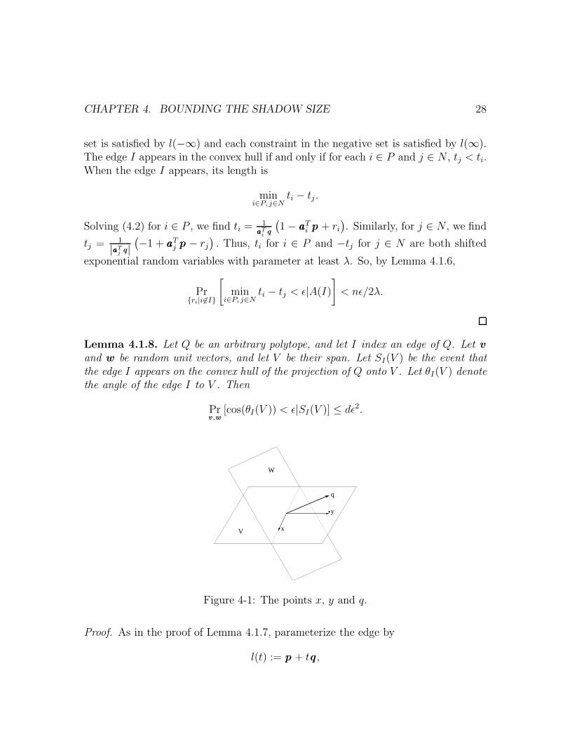
Lemma 4.1.8. Let Q be an arbitrary polytope, and let I index an edge of Q. Let v
and w be random unit vectors, and let V be their span. Let SI(V ) be the event thatthe edge I appears on the convex hull of the projection of Q onto V . Let θI(V ) denotethe angle of the edge I to V . Then
Prv ,w
[cos(θI(V )) < ε|SI(V )] ≤ dε2.
xV
q
y
W
Figure 4-1: The points x, y and q.
Proof. As in the proof of Lemma 4.1.7, parameterize the edge by
l(t) := p + tq ,

CHAPTER 4. BOUNDING THE SHADOW SIZE 29
where q is a unit vector. Observe that SI(V ) holds if and only if V non-triviallyintersects the cone
∑i∈I αiaaai|αi ≥ 0
, which we denote C. To evaluate the proba-
bility, we will perform a change of variables that will both enable us to easily evaluatethe angle between q and V and to determine whether SI(V ) holds. Some of the newvariables that we introduce are shown in Figure 4-1.
First, let W be the span of aaai|i ∈ I, and note that W is also the subspaceorthogonal to q . The angle of q to V is determined by the angle of q to the unitvector through the projection of q onto V , which we will call y . Fix any vector c ∈ C,and let x be the unique unit vector in V that is orthogonal to y and has positiveinner product with c. Note that x is also orthogonal to q , and so x ∈ V ∩ W . Alsonote that SI(V ) holds if and only if x ∈ C.
Instead of expressing V as the span of v and w , we will express it as the span ofx and y , which are much more useful vectors. In particular, we need to express v
and w in terms of x and y , which we do by introducing two more variables, α andβ, so that
v = x cos α + y sin α, and
w = x cos β + y sin β.
Note that number of degrees of freedom has not changed: v and w each had d − 1degrees of freedom, while x only has d − 2 degrees of freedom since it is restrictedto be orthogonal to q , and given x , y only has d − 2 degrees of freedom since it isrestricted to be orthogonal to x .
We now make one more change of variables so that the angle between q and y
becomes a variable. To do this, we let θ = θI(V ) be the angle between y and q ,and note that once θ and x have been specified, y is constrained to lie on a d − 2dimensional sphere. We let z denote the particular point on that sphere.
Deshpande and Spielman [16, Full version] prove that the Jacobian of this changeof variables from v and w to α, β, x , θ, z is
c(cos θ)(sin θ)d−3 sin(α − β)d−2,
where c is a constant depending only on the dimension.
CHAPTER 4. BOUNDING THE SHADOW SIZE 30
We now compute
PrV
[cos(θI(V )) < ε|SI(V )]
=
∫v ,w∈Sn−1:V ∩C 6=∅ and θI(V )≤ε
1 dv dw∫v ,w∈Sn−1:Span(v ,w)∩C 6=∅ 1 dv dw
=
∫θ>cos−1(ε),x∈C,z ,α,β
c(cos θ)(sin θ)d−3 sind−2(α−β) dx dz dα dβ dθ∫x∈C,θ,z ,α,β
c(cos θ)(sin θ)d−3 sind−2(α−β) dx dz dα dβ dθ
=
∫ π/2
θ=cos−1(ε)(cos θ)(sin θ)d−3 dθ
∫ π/2
θ=0(cos θ)(sin θ)d−3 dθ
=(sin θ)d−2
∣∣π/2
cos−1(ε)
(sin θ)d−2∣∣π/2
0
≤ 1 − (sin(cos−1(ε))d−2
≤ 1 − (1 − ε2)(d−2)/2 ≤ d − 2
2ε2.
Lemma 4.1.9. For all I ∈(
[n]d−1
),
EV,r1,...,rn[`(I)|SI(V )] ≥ λ
6√
dn.
Proof. For each edge I, `(I) = δ(I) cos(θI(V )). Lemma 4.1.7 now implies that,
Pr
[δ(I) ≥ λ
n
∣∣∣ A(I)
]≥ 1/2.
By Lemma 4.1.8,
PrV
[cos(θI(V )) ≥ 1/
√2d∣∣∣ SI(V )
]≥ 1/2.
Given that edge I appears on the shadow, it follows that `(I) > (1/√
2d)(
λn
)with
probability at least 1/4. Thus, its expected length when it appears is at least λ6√
dn.
4.2 The Shadow Size in the General Case
In this section, we present an extension of Theorem 4.1.2 that we will require in theanalysis of our simplex algorithm. We extend the theorem in two ways. First of

CHAPTER 4. BOUNDING THE SHADOW SIZE 31
all, we examine what happens when P is not k-round position. In this case, we justshow that the shadow of the convex hull of the vertices of bounded norm probablyhas few edges. As such, if we take a polynomial number of steps around the shadow,we should either come back to where we started or find a vertex far from the origin.Secondly, we consider the shadow onto random planes that come close to a particularvector, rather than just onto uniformly random planes.
Definition 4.2.1. For a unit vector u and a ρ > 0, we define the ρ-perturbation ofu to be the random unit vector v chosen by
1. choosing a θ ∈ [0, π] according to the restriction of the exponential distributionof expectation ρ to the range [0, π], and
2. setting v to be a uniformly chosen unit vector of angle θ to u .
Theorem 4.2.2. Let aaa1, . . . ,aaan be vectors of norm at most 1. Let r1, . . . , rn beindependent exponentially distributed random variables with expectation λ. Let Q bethe polytope given by
Q =x |∀i, aaaT
i x ≤ 1 + ri
.
Let u be an arbitrary unit vector, ρ < 1/√
d, and let v be a random ρ perturbation ofu . Let w be a uniformly chosen random unit vector. Then, for all t > 1,
Er1,...,rn,v ,w
[ShadowSizespan(v ,w)(Q ∩ B(0 , t))
]≤ 42πt(1 + λ log n)
√dn
λρ.
Proof. The proof of Theorem 4.2.2 is almost identical to that of Theorem 4.1.2, exceptthat we substitute Lemma 4.2.3 for Lemma 4.1.7, and we substitute Lemma 4.2.4 forLemma 4.1.8.
Lemma 4.2.3. For I ⊆(
[n]d−1
)and t > 0,
Pr[δ(I) < ε
∣∣A(I) and I ∩ B(0 , t) 6= ∅]≤ nε
2λ.
Proof. The proof is identical to the proof of Lemma 4.1.7, except that in the proof ofLemma 4.1.6 we must condition upon the events that
r+ ≥ −√
t − ‖p‖ and r− ≤√
t − ‖p‖.
These conditions have no impact on any part of the proof.
CHAPTER 4. BOUNDING THE SHADOW SIZE 32
Lemma 4.2.4. Let Q be an arbitrary polytope, and let I index an edge of Q. Let u
be any unit vector, let ρ < 1/√
d, and let v be a random ρ perturbation of u . Let w
be a uniformly chosen random unit vector, and let V = span(u , v). Then
Prv ,w
[cos(θI(V )) < ε|SI(V )] ≤ 3.5ε2/ρ2.
Proof. We perform the same change of variables as in Lemma 4.1.8.To bound the probability that cos θ < ε, we will allow the variables x , z , α and
β to be fixed arbitrarily, and just consider what happens as we vary θ. To facilitatewriting the resulting probability, let µ denote the density function on v . If we fix x ,z , α and β, then we can write v as a function of θ. Moreover, as we vary θ by φ, v
moves through an angle of at most φ. So, for all φ < ρ and θ,
µ(v(θ)) < µ(v(θ + φ))/e. (4.3)
With this fact in mind, we compute the probability to be
∫v ,w∈Sn−1:V ∩C 6=∅ and θI (V )≤ε
µ(v) dv dw∫v ,w∈Sn−1:V ∩C 6=∅ µ(v) dv dw
≤ maxx ,z ,α,β
∫ π/2
θ=cos−1(ε)(cos θ)(sin θ)d−3µ(v(θ)) dθ
∫ π/2
θ=0(cos θ)(sin θ)d−3µ(v(θ)) dθ
≤ maxx ,z ,α,β
∫ π/2
θ=cos−1(ε)(cos θ)(sin θ)d−3µ(θ) dθ
∫ π/2
θ=π/2−ρ(cos θ)(sin θ)d−3µ(θ) dθ
≤e∫ π/2
θ=cos−1(ε)(cos θ)(sin θ)d−3 dθ
∫ π/2
θ=π/2−ρ(cos θ)(sin θ)d−3 dθ
, by (4.3)
= e(sin θ)d−2
∣∣π/2
cos−1(ε)
(sin θ)d−2∣∣π/2
π/2−ρ
= e1 − (sin(cos−1(ε))d−2
1 − (sin(ρ)d−2
≤ e1 − (1 − ε2)(d−2)/2
1 − (1 − ρ2/2)d−2
≤ e(d − 2)ε2
(d − 2)4(1 − 1/√
e)ρ2, as ρ < 1/
√d,
≤ 3.5(ε/ρ)2.

CHAPTER 4. BOUNDING THE SHADOW SIZE 33
Chapter 5
Reduction of Linear Programming
to Certifying Boundedness
5.1 Reduction to a Feasibility Problem
We now recall an old trick [45, p. 125] for reducing the problem of solving a linearprogram in form (1.1) to a different form that will be more useful for our purposes.We recall that the dual of such a linear program is given by
minimize b · y (5.1)
subject to ATy = c, y ≥ 0,
and that when the programs are both feasible and bounded, they have the samesolution. Thus, any feasible solution to the system of constraints
Ax ≤ b, x ∈ Rd, (5.2)
ATy = c, y ≥ 0 ,
c · x = b · y
provides a solution to both the linear program and its dual. Since solving the abovesystem is trivial if b is the zero vector, we assume from here on in that b 6= 0 .
By introducing a new vector of variables δ ∈ Rd, we can replace the matrixinequality Ax ≤ b by an equality constraint and a nonnegativity constraint:
Ax + δ = b
δ ≥ 0 .
Now the variables δi and yi are constrained to be nonnegative, whereas each xi may be
34
CHAPTER 5. REDUCTION TO CERTIFYING BOUNDEDNESS 35
positive or negative. We would like to convert our system so that all of our variablesare constrained to be nonnegative. To do this, we replace each variable xi by a pairof variables, x+
i and x−i , each of which is constrained to be nonnegative. We then
replace every occurrence of the variable xi with the difference x+i − x−
i . It is notdifficult to see that, at any finite optimum, one of the two variables will be zero andthe other will equal the magnitude of the value that xi would have assumed at theoptimum of the original system.
Collecting all of our variables into one vector z 1 now gives us a feasibility problemof the form
AT1 z 1 = b1 (5.3)
z 1 ≥ 0 , z 1 6= 0
where A1 is a matrix constructed from A, b, and c, and the vector b1 is not the zerovector. If aaa
(1)1 , . . . ,aaa
(n)1 are the rows of A1, expressed as column vectors, we can write
this as
∑i≥1 z1,iaaa
(i)1 = b1 (5.4)
z 1 ≥ 0 , z 1 6= 0 .
Lemma 5.1.1. Solving the system in (5.4) can be reduced in polynomial time tosolving a system of the form
AT2 z 2 = 0 (5.5)
z 2 ≥ 0 , z 2 6= 0 .
Proof. Suppose that the bit-length required to express the system in (5.4) is L. Itis a standard fact in the analysis of linear programs that if (5.4) has a solution thenthere is a value κ = κ(L) that is singly-exponential in L so that (5.4) has a solutionwith ||z 2||1 < κ [50]. Using this value of κ, add a new coordinate z2,0 and form thesystem
−z2,0b1 +∑
i≥1 z2,i
(aaa
(i)1 − 1
κb1
)= 0 (5.6)
z 2 ≥ 0 , z 2 6= 0 .
We claim that the system in (5.6) is feasible if and only if the system in (5.4) is.

CHAPTER 5. REDUCTION TO CERTIFYING BOUNDEDNESS 36
To see this, first suppose that z 1 is a solution to the system in (5.4), and let
z2,i =
z1,i for i ≥ 1
1 − 1κ||z 1||1 for i = 0.
Clearly z 2 ≥ 0 and z 2 6= 0 , so we just have to check the equality constraint:
−z2,0b1 +∑
i≥1
z2,i
(aaa
(i)1 − 1
κb1
)= −
(1 − 1
κ||z 1||1
)b1 +
∑
i≥1
z1,i
(aaa
(i)1 − 1
κb1
)
= −(
1 − 1
κ||z 1||1
)b1 + b1 −
1
κ||z 1||1b1
= 0,
as desired.Conversely, suppose that z 2 is a solution to the system in (5.5). By definition
z 2 6= 0, so it is well-defined to set
z1,i = z2,i
(z2,0 +
1
κ
∑
j≥1
z2,j
)−1
for all i ≥ 1. Clearly z 1 ≥ 0 and z 1 6= 0 , so we again need only check the equalityconstraint:
∑
i≥1
z1,iaaa(i)1 =
(z2,0 +
1
κ
∑
j≥1
z2,j
)−1∑
i≥1
z2,iaaa(i)1
=
(z2,0 +
1
κ
∑
j≥0
z2,j
)−1(z2,0 +
1
κ
∑
k≥1
z2,k
)b1
= b1,
where the second equality follows from the equality constraint in (5.6). This completesthe proof of Lemma 5.1.1.

CHAPTER 5. REDUCTION TO CERTIFYING BOUNDEDNESS 37
5.2 Degeneracy and the Reduction to Certifying
Boundedness
LetR = w |A2w ≤ 1, (5.7)
and let aaa(0)2 , . . . ,aaa
(n)2 be the rows of A2. A feasible solution z to the system in (5.5)
is a nontrivial positive combination of the rows of A2 that equals the zero vector.Scaling the coefficients will give us a convex combination of the aaa
(i)2 that equals the
zero vector. Since the polar polytope R∗ is the convex hull of the aaa(i)2 , the system
in (5.5) is thus feasible if and only if the origin is contained in R∗.We recall from Section 2.4 that R is bounded if and only if R∗ contains the origin
in its interior. By Remark 2.4.3, a feasible solution to the system in (5.5) is thusquite close to a certificate of boundedness for R; they differ only in the degeneratecase when the origin appears on the boundary of R∗. In this section, we shall use aprocedure similar to the ε-perturbation technique of Charnes [11] and Megiddo andChandrasekaran [40] to reduce solving (5.5) to solving it in the nonndegenerate case,where a solution to (5.5) is equivalent to a certificate of boundedness for R.
Let A2 be an m × n matrix. By restricting to a subspace if necessary, we canassume that the rows of A2 span Rn so that R∗ is a full-dimensional polytope, andour problem is to determine whether the origin lies in the polytope. We shall nowperturb our problem slightly by pushing to origin very slightly toward the average ofthe aaa
(i)2 . More precisely, we shall seek a feasible solution to the system
AT2 (q − ε (
∑i qi/m)1) = 0 (5.8)
q ≥ 0 , q 6= 0 ,
where ε = 1/2poly(m)·L with a sufficiently large polynomial in the exponent. We canwrite this in the same form as the system in (5.5) by letting A3 be the matrix whoseith row is given by
aaa(i)3 = aaa
(i)2 − ε
m
∑
i
aaa(i)2 (5.9)
and considering the system
AT3 q = 0
q ≥ 0 , q 6= 0 .
We claim that this yields a polynomial-time reduction to the nondegenerate case.This follows from the following four properties of the system in (5.8):

CHAPTER 5. REDUCTION TO CERTIFYING BOUNDEDNESS 38
Property 1: Given the system in (5.5), we can construct the system in (5.8) inpolynomial time.
Property 2: If (5.5) is feasible then (5.8) has a solution whose coordinates are allstrictly positive.
Property 3: If (5.5) is infeasible then (5.8) is infeasible.
Property 4: Given a solution to (5.8), one can recover a solution to (5.5) in poly-nomial time.
Proof of Property 1. This follows immediately from the description of the systemin (5.8) and the fact that the bit-length of ε is polynomial in L.
Proof of Property 2. Let q be a feasible point for (5.5), so that
AT2 q = 0 .
Let
q = q +ε∑
i qi
m(1 − ε)1.
We note that q is a feasible solution to (5.8):
AT2
(q − ε
(∑
i
qi/m
)1
)= AT
2
((q +
ε∑
i qi
m(1 − ε)1
)− ε
m
(∑
i
qi +εm∑
i qi
m(1 − ε)
)1
)
= AT2 q + AT
2
((ε∑
i q
m(1 − ε)− ε
m
(1 +
ε
1 − ε
)∑
i
qi
)1
)
= 0 +
(ε
m(1 − ε)− ε
m
(1 − ε) + ε
1 − ε
)(∑
i
qi
)AT
2 1
= 0 + 0
(∑
i
qi
)AT
2 1 (5.10)
= 0 ,
as desired. Since all of the coefficients of q are strictly positive, this establishesProperty 2.
Proof of Property 3. Let aaa(i)3 be as in equation (5.9). The system in (5.5) is feasible
if and only if the origin is contained in the convex hull R∗ of the aaa(i)2 , whereas the

CHAPTER 5. REDUCTION TO CERTIFYING BOUNDEDNESS 39
system in (5.8) is feasible if and only if the origin is contained in the convex hull of
the aaa(i)3 .
Suppose that (5.5) is infeasible; we show that this implies that (5.8) is infeasibleas well. To this end, let p ∈ R∗ be the point on R∗ that is closest to the origin. Thepoint p lies on the boundary of R∗, so there exists some collection of n of the aaa
(i)2
that spans a nondegenerate simplex ∆ that contains p. Without loss of generality,let this collection consist of aaa
(1)2 , . . . ,aaa
(n)2 . Let
∆ = conv(∆,0 ).
The n-dimensional volume of ∆ equals 1/n times the (n − 1)-dimensional volume of∆ times the orthogonal distance from the hyperplane spanned by ∆ to the origin.We thus have
||p||2 ≥n · voln(∆)
voln−1(∆).
If M1 is the n×n matrix whose ith row equals aaa(i)T2 , and M2 is the (n− 1)×n matrix
whose ith row equals aaa(i)2 − aaa
(n)2 , we can expand this as
||p||2 ≥ n · voln(∆)
voln−1(∆)
=n · (1/n!)
√det (MT
1 M1)
(1/(n − 1)!)√
det (MT2 M2)
(5.11)
=
√det (MT
1 M1)
det (MT2 M2)
.
All of entries in M1 and M2 have bit-lengths that are bounded above by L, so thenumerator and denominator of the fraction under the square root can both be writtenwith poly(m) · L bits, and thus so can the entire fraction. Since we have assumedthat ||p||2 6= 0, this implies a 1/2poly(m)·L lower bound on ||p||2.
We thus have a lower bound ` on the distance between the convex hull of the aaa(i)2
and the origin. If we displace each aaa(i)2 by less than `, no convex combination of the
aaa(i)2 can move by more than `, so the perturbed polytope will not contain the origin.
The distance between aaa(i)2 and aaa
(i)3 is at most
ε
m
∣∣∣∣∣
∣∣∣∣∣
(∑
i
aaa(i)2
)∣∣∣∣∣
∣∣∣∣∣2
,
CHAPTER 5. REDUCTION TO CERTIFYING BOUNDEDNESS 40
so, as long as
ε <`m∣∣∣
∣∣∣(∑
i aaa(i)2
)∣∣∣∣∣∣2
= Ω
(1
2poly(m)·L
),
the convex hull of the aaa(i)3 will not contain the origin. This implies the infeasibility
of (5.8), as desired.
Proof of Property 4. Given any solution to (5.8), standard techniques allow one torecover, in polynomial time, a solution at which exactly n of the qi are nonzeroand for which the corresponding aaa
(i)3 are linearly independent [45]. Scaling so that
the coefficients add to 1, this shows that the origin is contained inside the simplexspanned by n of the aaa
(i)3 . The proof of Property 3 shows that the simplex spanned by
the corresponding aaa(i)2 will also contain the origin, i.e., that the origin can be written
as a convex combination of the corresponding aaa(i)2 . We can find the coefficients of this
convex combination in polynomial time by solving a linear system, and this is ourdesired solution.
It thus suffices to be able to find a certificate of boundedness for the polytopedescribed in (5.7). This is equivalent to proving that
A2w ≤ b2 (5.12)
is bounded for any b2 > 0 , since the choice of the vector b2 does not affect whetherthe polytope is bounded. (We require b2 > 0 in order to guarantee that the resultingsystem is feasible.) By solving this system with a randomly chosen right-hand sidevector we can solve system (1.1) while avoiding the combinatorial complications ofthe feasible set of (1.1).
In our algorithm, we will certify boundedness of (1.1) by finding the verticesminimizing and maximizing some objective function. Provided that the system isnon-degenerate, which it is with high probability under our choice of right-hand sides,this can be converted into a solution to (5.5).
Chapter 6
Our Algorithm
Our bound from Theorem 4.1.2 suggests a natural algorithm for certifying the bound-edness of a linear program of the form given in (5.12): set each bi to be 1+ri, where ri
is an exponential random variable, pick a random objective function c and a randomtwo-dimensional subspace containing it, and then use the shadow-vertex method withthe given subspace to maximize and minimize c.
In order to make this approach into a polynomial-time algorithm, there are twodifficulties that we must surmount:
1. To use the shadow-vertex method, we need to start with some vertex thatappears on the boundary of the shadow. If we just pick an arbitrary shadowplane, there is no obvious way to find such a vertex.
2. Theorem 4.1.2 bounds the expected shadow size of the vertices of bounded normin polytopes with perturbed right-hand sides, whereas the polytope that we aregiven may have vertices of exponentially large norm. If we naively choose ourperturbations, objective function, and shadow plane as if we were in a coordinatesystem in which all of our vertices had bounded norm, the distribution of verticesthat appear on the shadow may be very different, and we have no guaranteesabout the expected shadow size.
We address the first difficulty by constructing an artificial vertex at which to startour simplex algorithm. To address the second difficulty, we start out by choosing ourrandom variables from the naive distributions. If this doesn’t work, we iteratively useinformation about how it failed to improve the probability distributions from whichwe sample and try again.
41
CHAPTER 6. OUR ALGORITHM 42
6.1 Constructing a Starting Vertex
In order to use the shadow-vertex method on a polytope P , we need a shadow plane S
and a vertex v that appears on the boundary of the shadow. One way to obtain sucha pair is to pick any vertex v , randomly choose (from some probability distribution)an objective function c optimized by v , let u be a uniformly random unit vector, andset S = span(c,u).
However, to apply the bound on the shadow size given by Theorem 4.2.2, we needto choose c to be a ρ-perturbation of some vector. For such a c to be likely to beoptimized by v , we need v to optimize a reasonably large ball of objective functions.To guarantee that we can find such a v , we create one. That is, we add constraintsto our polytope to explicitly construct an artificial vertex with the desired properties.(This is similar to the “Phase I” approaches that have appeared in some other simplexalgorithms.)
Suppose for now that the polytope x |Ax ≤ 1 is k-round. Construct a modifiedpolytope P ′ by adding d new constraints,
wT
i x ≤ 1, i = 1, . . . , d, where
w i = −(∑
j
ej
)+√
de i/3k2,
and w i = w i/(2 ||w i||). Let x 0 be the vertex at which w 1, . . . ,w d are all tight.Furthermore, let c be a ρ-perturbation of the vector 1/
√d, with ρ = 1/6dk2, and let
x 1 be the vertex at which c is maximized. We can prove:
Lemma 6.1.1. The following three properties hold with high probability. Further-more, they remain true with probability 1 − (d + 2)e−n if we perturb all of the right-hand sides of the constraints in P ′ by an exponential random variable of expectationλ = 1/n.
1. The vertex x 0 appears on P ′,
2. −c is maximized at x 0, and
3. None of the constraints w 1, . . . ,w d is tight at x 1.
Proof. This follows from Lemma 7.0.1 and bounds on tails of exponential randomvariables.
Setk := 16d + 1 and s := 4 · 107 d9/2n.
Let S = span(c,u), where u is a uniform random unit vector. If P is k-round, thenby Lemma 6.1.1 and Theorem 4.1.2 we can run the shadow vertex method on P ′
CHAPTER 6. OUR ALGORITHM 43
with shadow plane S and starting at vertex x 0, and we will find the vertex x 1 thatmaximizes c within s steps, with probability at least 1/2. Since none of the w i aretight at x 1, x 1 will also be the vertex of the original polytope P that maximizes c.
This gives us the vertex x 1 of P that maximizes c. We can now run the shadowvertex method again on P using the same shadow plane. This time, we start at x 1
and find the vertex that maximizes −c. We are again guaranteed to have an expectedpolynomial-sized shadow, so this will again succeed with high probability. This willgive us a pair of vertices that optimize c and −c, from which we can compute ourdesired certificate of boundedness. It just remains to deal with polytopes that arenot k-round position.
6.2 Polytopes that are not k-Round
In this section, we shall present and analyze our general algorithm that deals withpolytopes that may not be k-round. The pseudocode for this algorithm appears atthe end of the section, on page 46.
We first observe that for every polytope there exists an affine change of coordinates(i.e., a translation composed with a change of basis) that makes it d-round [5]. Anaffine change of coordinates does not change the combinatorial structure of a polytope,so this means that there exists some probability distribution on b and S for whichthe shadow has polynomial expected size. We would like to sample b and S fromthese probability distributions and then pull the result back along the change ofcoordinates. Unfortunately, we don’t know an affine transformation that makes ourpolytope k-round, so we are unable to sample from these distributions.
Instead, we shall start out as we would in the k-round case, adding in artificialconstraints w 1, . . . ,w d, and choosing an objective function and shadow plane as inSection 6.1. By Theorem 4.2.2, running the shadow-vertex method for s steps willyield one of two results with probability at least 1/2:
1. It will find the optimal vertex x 1, or
2. It will find a vertex y of norm at least 2k.
In the first case, we can proceed just as in the k-round case and run the shadow-vertexmethod a second time to optimize −c, for which we will have the same two cases.
In the second case, we have not found the optimal vertex, but we have with highprobability learned a point of large norm inside our polytope. We can use this pointto change the probability distributions from which we draw our random variables andthen start over. This changes our randomized pivot rule on the graph of potentialvertices of our polytope, hopefully putting more probability mass on short paths from
CHAPTER 6. OUR ALGORITHM 44
the starting vertex to the optimum. We shall show that, with high probability, weneed only repeat this process a polynomial number of times before we find a right-hand side and shadow plane for which the shadow-vertex method finds the optimum.
Our analysis rest upon the following geometric lemma, proved in Chapter 7:
Lemma 6.2.1. Let B ⊆ Rd be the unit ball, let P be a point at distance S from the
origin, and let C = conv(B, P ) be their convex hull. If S ≥ 16d + 1, then C containsan ellipse of volume at least twice that of B, having d−1 semi-axes1 of length 1−1/dand one semi-axis of length at least 8 centered at the point of distance 7 from theorigin in the direction of P .
We remark that the number of times that we have to change probability distri-butions depends on the bit-length of the inputs, and that this is the only part ofour algorithm in which this is a factor. Otherwise, the execution of our algorithm istotally independent of the bit-length of the inputs.
Theorem 6.2.2. If each entry of the vectors aaai is specified using L bits, thenCheckBoundedness() either produces a certificate that its input is bounded or thatit is unbounded within O(n3L) iterations, with high probability.
Proof. It will be helpful to think of the input to CheckBoundedness() as beingthe polytope
x |aaaT
i x ≤ 1 ∀i
instead of just the vectors aaa1, . . . ,aaan. We can then talkabout running this algorithm on an arbitrary polytope
x |αT
i x ≤ τi ∀i
by rewritingthis polytope as
x | (αi/τi)
T x ≤ 1 ∀i.
With this notation, it is easy to check that running an iteration of the Repeat
loop on a polytope P with Q = Q0 and r = r 0 is equivalent to running the samecode on the polytope Q0(P + r 0) with Q = Id and r = 0. The update step atthe end of the algorithm can therefore be thought of as applying an affine change ofcoordinates to the input and then restarting the algorithm.
If Q = Idn and r = 0, the argument from Section 6.1 proves that the first iterationof the Repeat loop will either prove boundedness, prove unboundedness, or find apoint with norm at least k with probability at least 1/2. In either of the first twocases, the algorithm will have succeeded, so it suffices to consider the third.
If a point y is in the polytope P ′ = x |Ax ≤ b, the point y/2 will be in thepolytope P = x |Ax ≤ 1 with probability at least 1 − ne−n. This guarantees thatP contains a point of norm at least k. Since P contains the unit ball, Lemma 6.2.1implies that P contains an ellipse of volume at least twice that of the unit ball. The
1If an ellipsoid E is given as the set E =x |xT Q−1x ≤ 1
, where Q is a symmetric, positive
definite matrix, then the semi-axes of E have lengths equal to the the eigenvalues of Q. For example,
the semi-axes of the sphere are all of length 1.

CHAPTER 6. OUR ALGORITHM 45
update step of our algorithm identifies such an ellipse and scales and translates sothat it becomes the unit ball, and it then restarts with this new polytope as its input.This new polytope has at most half the volume of the original polytope.
All the vertices of the original polyhedron are contained in a ball of radius 2O(n2L),where L is the maximum bit-length of any number in the input, and so their convexhull has volume at most 2O(n3L) times that of the unit ball [26]. Each iteration of thealgorithm that finds a point of norm at least k decreases the volume of P by a factorof at least 2. All of the polytopes that we construct contain the unit ball, so this canoccur at most O(n3L) times. This guarantees that the Repeat loop finds an answerafter a O(n3L) iterations with high probability, as desired.
While the algorithm requires samples from the exponential distribution and uni-form random points on the unit sphere, it is not difficult to show that it suffices touse standard discretizations of these distributions of bit-length polynomial in n andd.

CHAPTER 6. OUR ALGORITHM 46
Algorithm 6.2.1: CheckBoundedness(aaa1, . . . ,aaan)
Require each aaai has norm at most 1.Set k = 16d + 1, λ = 1/n, ρ = 1/6dk2
s = 4 · 107 d9/2n, and w i as described in text;Initialize Q := Idn, r := 0;Repeat until you return an answer
Construct constraints for starting corner:aaan+i := QTw i/(1 − w i · (Qr)) for i = 1, . . . , d;
bi := (1 + βi)(1 + aaaTi r) for i = 1, . . . n + d, (1)
βi exponential random vars with expectation λ;Set starting corner x 0 := point where aaaT
i x 0 = bi
for i = n + 1, . . . , n + d;If x 0 violates aaaT
i x 0 ≤ bi for any i, go back to (1)and generate new random variables;
c := QT γ, with γ a ρ-perturbation of 1/√
d;Shadow plane S := span(c,QTu),
with u a uniformly random unit vector;Run ShadowVertex((aaa1, . . . ,aaan+d), b, c,S , x 0, s) :
If returns unbounded then
return (unbounded);If returns (fail, y 0) then
set y := y0 and go to (3);If returns (opt, v 0) then
set v := v 0 and continue to (2);Run ShadowVertex((aaa1, . . . ,aaan), b, c,S , v , s) : (2)
If returns unbounded then
return (unbounded);If returns (fail, y 0) then
set y := y 0 and go to (3);If returns (opt, v 0) then
set v ′ := v 0 and return (v , v ′);Update Q and r : (3)
If ||Q(y + r)|| ≤ 2k then
don’t change Q or r
else
Set M := the matrix that scales downQ(y + r) by factor of 8 and scalesvectors in orthogonal complement upby factor of 1 − 1/d;
Q := MQ ;r := r + 7Q(y + r)/||Q(y + r)||;

CHAPTER 6. OUR ALGORITHM 47
6.3 Towards a Strongly Polynomial-Time Algorithm
for Linear Programming?
While it is usually best to avoid the risky business of predicting yet-unproven results,it is worth briefly noting that we believe these results to be encouraging progresstowards finding a strongly polynomial-time algorithm for linear programming.
First of all, these results provide significant geometric insights into the structureof linear programming and polytope theory, and they provide a new approach to con-structing algorithms for linear programming. Our algorithm proceeds almost entirelyin strongly polynomial time, and it runs in strongly polynomial time for a large classof linear programs. The only part of the algorithm that is not strongly polynomial isthe outer loop in which we alter the various probability distributions. It seems quiteplausible that this dependence can be eliminated by a slightly more clever variant ofour algorithm.
Furthermore, our methods suggest a wide variety of similar approaches. Whilethe shadow-vertex method was the easiest simplex method to analyze, it may wellbe the worst one to use when searching for a strongly polynomial-time algorithm.The dependence of the running-time of the algorithm on the bit-length arises fromthe linear program being given initially in a “bad” coordinate system. The shadow-vertex method is perhaps, among reasonable pivot rules, the one that depends themost adversarially upon the ambient coordinate system. If one could obtain a similaranalysis of the behavior on linear programs with perturbed right-hand sides of a lesscoordinate-dependent pivot rule, such as RANDOM-EDGE (see [23], for example), itis quite possible that the dependence on the bit-length would disappear.
Chapter 7
Geometric Lemmas for Algorithm’s
Correctness
Lemma 7.0.1. Let P be a k-round polytope, let c and q be unit vectors, and let
v = argmaxx∈P
c · x
be the vertex of P at which c ·x is maximized. If c · q ≤ −(2k2−1)/2k2, then v · q ≤ 0.
Proof. We first note that
||q + c||2 = ||q||2 + ||c||2 + 2(c · q) ≤ 2 − 2k2 − 1
k2=
1
k2,
so ||q + c|| ≤ 1/k. The fact that P is contained in B(0, k) implies that ||v|| ≤ k, andthe fact that P contains the unit ball implies that
v · c = maxx∈P
c · x ≥ 1.
We therefore have
q · v = −c · v + (q + c) · v ≤ −1 + ||q + c||||v|| ≤ 0,
as desired.
We now prove some geometric facts that will be necessary for the analysis of ouralgorithm. We first prove a two-dimensional geometric lemma. We then use this toprove a higher-dimensional analogue, which is the version that we shall actually useto analyze our algorithm.
48
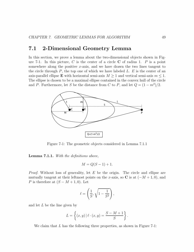
CHAPTER 7. GEOMETRIC LEMMAS FOR ALGORITHM 49
7.1 2-Dimensional Geometry Lemma
In this section, we prove a lemma about the two-dimensional objects shown in Fig-ure 7-1. In this picture, C is the center of a circle C of radius 1. P is a pointsomewhere along the positive x-axis, and we have drawn the two lines tangent tothe circle through P , the top one of which we have labeled L. E is the center of anaxis-parallel ellipse E with horizontal semi-axis M ≥ 1 and vertical semi-axis m ≤ 1.The ellipse is chosen to be a maximal ellipse contained in the convex hull of the circleand P . Furthermore, let S be the distance from C to P , and let Q = (1 − m2)/2.
C E
P
1 mS
M
Q=(1-m )/22
L
Figure 7-1: The geometric objects considered in Lemma 7.1.1
Lemma 7.1.1. With the definitions above,
M = Q(S − 1) + 1.
Proof. Without loss of generality, let E be the origin. The circle and ellipse aremutually tangent at their leftmost points on the x-axis, so C is at (−M + 1, 0), andP is therefore at (S − M + 1, 0). Let
` =
(1
S,
√1 − 1
S2
),
and let L be the line given by
L =
(x, y) | ` · (x, y) =
S − M + 1
S
.
We claim that L has the following three properties, as shown in Figure 7-1:
CHAPTER 7. GEOMETRIC LEMMAS FOR ALGORITHM 50
1. L passes through P .
2. L is tangent to C.
3. If we take the major semi-axis M of the ellipse E to be Q(S − 1) + 1, then L istangent to E.
Establishing these properties would immediately imply Lemma 7.1.1, so it suffices tocheck them one by one.
1. This follows by direct computation—we simply note that the point P = (S −M + 1, 0) satisfies the equation for L.
2. It suffices to show that the distance from the point C to the line L is exactly 1.Since L is the unit normal to L, it suffices to check that
` · C =
(S − M + 1
S
)− 1 =
−M + 1
S,
which again follows by direct computation.
3. Let
L = (Lx,Ly) =S
S − M + 1`
=
(1
S − M + 1,
√S2 − 1
S − M + 1
),
so that L = (x, y) | L · (x, y) = 1. When expressed in this form, L will betangent to E if and only if L2
xM2 +L2
ym2 = 1. This can be verified by plugging
in M = Q(S − 1) + 1 and Q = (1 − m2)/2, and then expanding the left-handside of the equation.
7.2 High-Dimensional Geometry Lemma
Lemma 7.2.1. Let B ⊆ Rd be the unit ball, let P be a point at distance S from theorigin, and let C = conv(B, P ) be their convex hull. For any m ≤ 1, C contains anellipsoid with (d−1) semi-axes of length m and one semi-axis of length (1 − m2) (S−1)/2 + 1.

CHAPTER 7. GEOMETRIC LEMMAS FOR ALGORITHM 51
Proof. Without loss of generality, take P = (S, 0, . . . , 0). Consider an axis-parallelellipsoid E with the axes described in the above theorem, with its distinct axis parallelto e1, and translated so that it is tangent to B at (−1, 0, . . . , 0).
We assert that E is contained in C. It suffices to check the containment when weintersect with an arbitrary 2-dimensional subspace containing 0 and P . In this case,we have exactly the setup of Lemma 7.1.1, and our result follows immediately.
of Lemma 6.2.1. If we set m = 1−1/d, then Lemma 7.2.1 guarantees that the lengthof the longer semi-axis of the ellipse will be at least
(1 −
(1 − 1
d
)2)
16d
2≥ 8.
So, the ratio of the volume of the unit ball to the ellipse is at least
V/vol(B) ≥(
1 − 1
d
)d−1
8
≥ 8
4= 2.
Part II
Spectral Partitioning, Eigenvalue
Bounds, and Circle Packings for
Graphs of Bounded Genus
52
Chapter 8
Background in Graph Theory and
Spectral Partitioning
In this chapter we provide the basic definitions and results from graph theory andspectral partitioning that we shall require in the sequel.
8.1 Graph Theory Definitions
Throughout the remainder of this part of the thesis, let G = (V, E) be a finite,connected, undirected graph with n vertices, m edges, and no loops. In this section,we shall define two objects associated to G: its Laplacian, and its genus.
Let the adjacency matrix A(G) be the n × n matrix whose (i, j)th entry equals 1if (i, j) ∈ E, and equals 0 otherwise. Let D(G) be the n × n diagonal matrix whoseith diagonal entry equals the degree of the ith vertex of G.
Definition 8.1.1. The Laplacian L(G) is the n × n matrix given by
L(G) = D(G) − A(G).
Since L(G) is symmetric, it is guaranteed to have an orthonormal basis of realeigenvectors and exclusively real eigenvalues. Let λ1 ≤ λ2 ≤ · · · ≤ λn be the eigenval-ues of L(G), and let v1, . . . , vn be a corresponding orthonormal basis of eigenvectors.For any G, the all-ones vector will be an eigenvector of eigenvalue 0. It is not dif-ficult to see that all of the other eigenvalues will always be nonnegative, so thatv1 = (1, . . . , 1)T , and λ1 = 0.
There has been a great deal of work relating the eigenvalues of L(G) to the struc-ture of G. In the present paper, we shall concern ourselves exclusively with λ2, alsoknown as the algebraic connectivity or Fiedler value of G. We call the vector v2 the
53
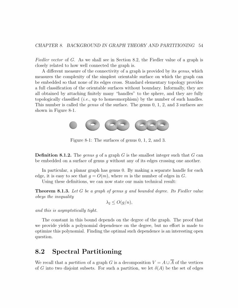
CHAPTER 8. BACKGROUND IN GRAPH THEORY AND PARTITIONING 54
Fiedler vector of G. As we shall see in Section 8.2, the Fiedler value of a graph isclosely related to how well connected the graph is.
A different measure of the connectivity of a graph is provided by its genus, whichmeasures the complexity of the simplest orientable surface on which the graph canbe embedded so that none of its edges cross. Standard elementary topology providesa full classification of the orientable surfaces without boundary. Informally, they areall obtained by attaching finitely many “handles” to the sphere, and they are fullytopologically classified (i.e., up to homeomorphism) by the number of such handles.This number is called the genus of the surface. The genus 0, 1, 2, and 3 surfaces areshown in Figure 8-1.
Figure 8-1: The surfaces of genus 0, 1, 2, and 3.
Definition 8.1.2. The genus g of a graph G is the smallest integer such that G canbe embedded on a surface of genus g without any of its edges crossing one another.
In particular, a planar graph has genus 0. By making a separate handle for eachedge, it is easy to see that g = O(m), where m is the number of edges in G.
Using these definitions, we can now state our main technical result:
Theorem 8.1.3. Let G be a graph of genus g and bounded degree. Its Fiedler valueobeys the inequality
λ2 ≤ O(g/n),
and this is asymptotically tight.
The constant in this bound depends on the degree of the graph. The proof thatwe provide yields a polynomial dependence on the degree, but no effort is made tooptimize this polynomial. Finding the optimal such dependence is an interesting openquestion.
8.2 Spectral Partitioning
We recall that a partition of a graph G is a decomposition V = A ∪A of the verticesof G into two disjoint subsets. For such a partition, we let δ(A) be the set of edges
CHAPTER 8. BACKGROUND IN GRAPH THEORY AND PARTITIONING 55
(i, j) such that i ∈ A and j ∈ A, and we call |δ(A)| the cut size of our partition. Theratio of our partition is defined to be
φ(A) =|δ(A)|
min(|A|, |A|).
If our partition splits the graph into two sets that differ in size by at most one, wecall it a bisection.
Spectral methods aim to use the Fiedler vector to find a partition of the graphwith a good ratio. A theorem that begins to address why these work was proven byMihail and restated in a more applicable form by Spielman and Teng:
Theorem 8.2.1 ([41, 47]). Let G have maximum degree ∆. For any vector x thatis orthogonal to the all-ones vector, there is a value s so that the partition of G intoi : xi ≤ s and i : xi > s has ratio at most
√2∆
xT L(G)x
xT x.
If x is an eigenvector of L(G), the fraction xT L(G)xxT x
is equal to its eigenvalue. So,if we find the eigenvector with eigenvalue λ2, we will thus quickly be able to find apartition of ratio
√2∆λ2. By Theorem 8.1.3, finding the second eigenvector of the
Laplacian thus allows us to find a partition of ratio O(√
g/n) for a graph of boundeddegree. There is no guarantee that this partition has a similar number of vertices ineach of the two sets. However, a theorem of Lipton and Tarjan [39] implies that asimple method based on repeated application of this algorithm can be used to give abisector of size O(
√gn).
For every g, Gilbert, Hutchinson, and Tarjan exhibited a class of bounded degreegraphs that have no bisectors smaller than O(
√gn) [25]. This implies that our al-
gorithm gives the best results possible, in general. Furthermore, it establishes theasymptotic tightness of our eigenvalue bound, as a smaller bound would show thatevery genus g graph has a partition of size o(
√gn).
Putting all of this together yields our main algorithmic result:
Theorem 8.2.2. Let G be a genus g graph of bounded maximum degree. There is apolynomial time algorithm that produces cuts of ratio O(
√g/n) and vertex bisectors
of size O(√
gn) in G, and both of these values are optimal.
All that remains of the proof of Theorem 8.2.2 is the eigenvalue bound set forthin Theorem 8.1.3, which is the goal of the remainder of this paper.
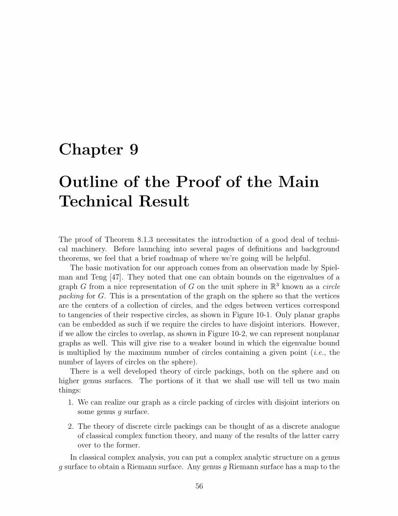
Chapter 9
Outline of the Proof of the Main
Technical Result
The proof of Theorem 8.1.3 necessitates the introduction of a good deal of techni-cal machinery. Before launching into several pages of definitions and backgroundtheorems, we feel that a brief roadmap of where we’re going will be helpful.
The basic motivation for our approach comes from an observation made by Spiel-man and Teng [47]. They noted that one can obtain bounds on the eigenvalues of agraph G from a nice representation of G on the unit sphere in R3 known as a circlepacking for G. This is a presentation of the graph on the sphere so that the verticesare the centers of a collection of circles, and the edges between vertices correspondto tangencies of their respective circles, as shown in Figure 10-1. Only planar graphscan be embedded as such if we require the circles to have disjoint interiors. However,if we allow the circles to overlap, as shown in Figure 10-2, we can represent nonplanargraphs as well. This will give rise to a weaker bound in which the eigenvalue boundis multiplied by the maximum number of circles containing a given point (i.e., thenumber of layers of circles on the sphere).
There is a well developed theory of circle packings, both on the sphere and onhigher genus surfaces. The portions of it that we shall use will tell us two mainthings:
1. We can realize our graph as a circle packing of circles with disjoint interiors onsome genus g surface.
2. The theory of discrete circle packings can be thought of as a discrete analogueof classical complex function theory, and many of the results of the latter carryover to the former.
In classical complex analysis, you can put a complex analytic structure on a genusg surface to obtain a Riemann surface. Any genus g Riemann surface has a map to the
56
CHAPTER 9. OUTLINE OF PROOF OF MAIN TECHNICAL RESULT 57
sphere that is almost everywhere k-to-one for k = O(g), with only O(g) bad pointsat which this fails. With this as motivation, we shall try to use the representation ofG as a circle packing on a genus g surface to obtain a representation of it as a circlepacking on the sphere with O(g) layers.
Unfortunately, the discrete theory is more rigid than the continuous one, and thiswill turn out to be impossible. Instead, we shall actually pass to the continuous theoryto prove our result. To do this, we shall provide a subdivision lemma that shows thatit suffices to prove Theorem 8.1.3 for graphs that have circle packings with very smallcircles. We shall then show that the smooth map that we have from the Riemannsurface to the sphere will take almost all of the circles of our circle packing to curveson the sphere that are almost circles. We will then show that this representation ofour graph as an approximate circle packing is enough to provide our desired bounds.
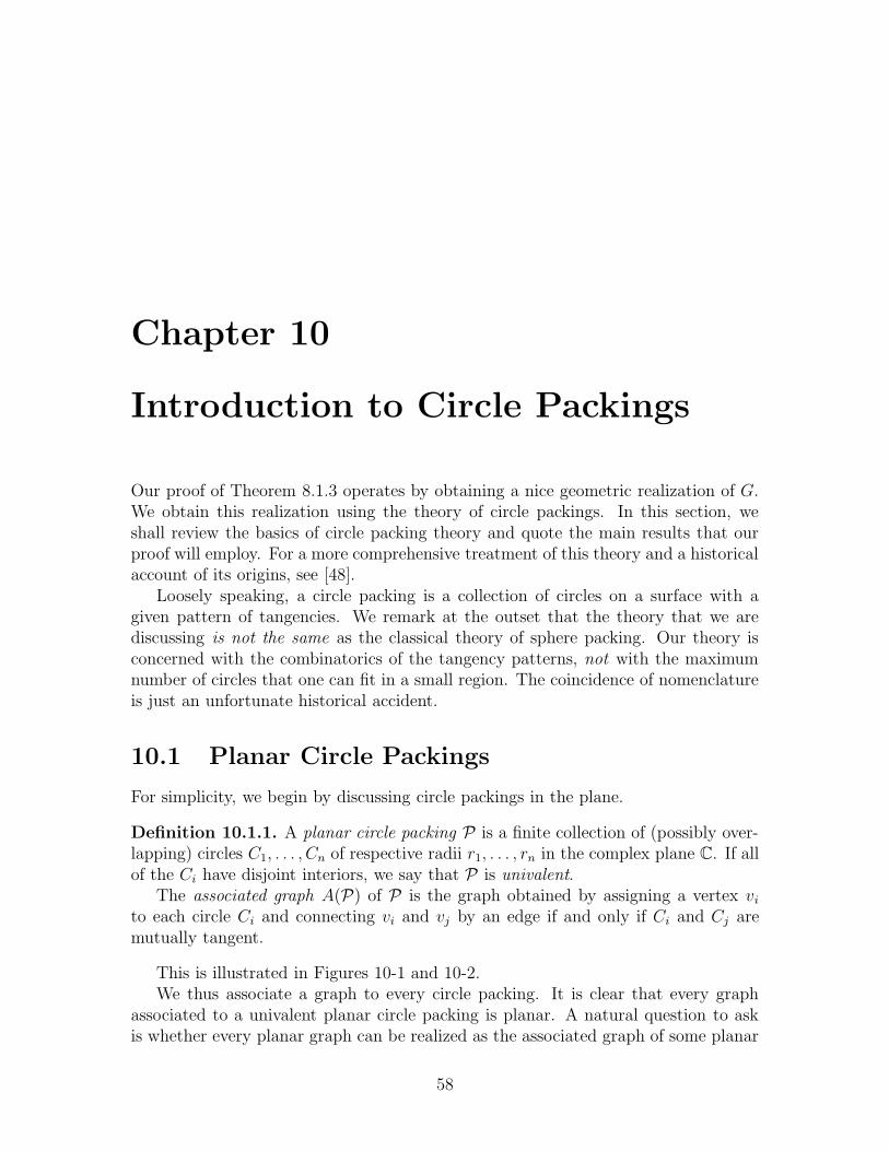
Chapter 10
Introduction to Circle Packings
Our proof of Theorem 8.1.3 operates by obtaining a nice geometric realization of G.We obtain this realization using the theory of circle packings. In this section, weshall review the basics of circle packing theory and quote the main results that ourproof will employ. For a more comprehensive treatment of this theory and a historicalaccount of its origins, see [48].
Loosely speaking, a circle packing is a collection of circles on a surface with agiven pattern of tangencies. We remark at the outset that the theory that we arediscussing is not the same as the classical theory of sphere packing. Our theory isconcerned with the combinatorics of the tangency patterns, not with the maximumnumber of circles that one can fit in a small region. The coincidence of nomenclatureis just an unfortunate historical accident.
10.1 Planar Circle Packings
For simplicity, we begin by discussing circle packings in the plane.
Definition 10.1.1. A planar circle packing P is a finite collection of (possibly over-lapping) circles C1, . . . , Cn of respective radii r1, . . . , rn in the complex plane C. If allof the Ci have disjoint interiors, we say that P is univalent.
The associated graph A(P) of P is the graph obtained by assigning a vertex vi
to each circle Ci and connecting vi and vj by an edge if and only if Ci and Cj aremutually tangent.
This is illustrated in Figures 10-1 and 10-2.We thus associate a graph to every circle packing. It is clear that every graph
associated to a univalent planar circle packing is planar. A natural question to askis whether every planar graph can be realized as the associated graph of some planar
58
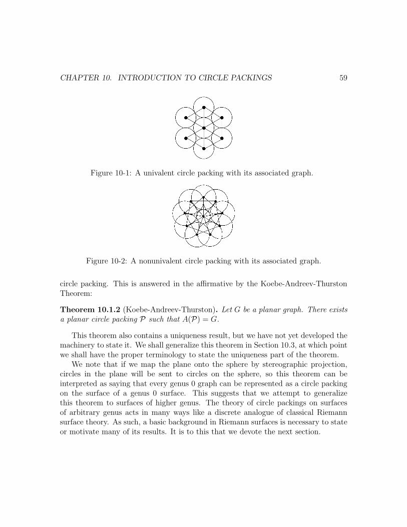
CHAPTER 10. INTRODUCTION TO CIRCLE PACKINGS 59
Figure 10-1: A univalent circle packing with its associated graph.
Figure 10-2: A nonunivalent circle packing with its associated graph.
circle packing. This is answered in the affirmative by the Koebe-Andreev-ThurstonTheorem:
Theorem 10.1.2 (Koebe-Andreev-Thurston). Let G be a planar graph. There existsa planar circle packing P such that A(P) = G.
This theorem also contains a uniqueness result, but we have not yet developed themachinery to state it. We shall generalize this theorem in Section 10.3, at which pointwe shall have the proper terminology to state the uniqueness part of the theorem.
We note that if we map the plane onto the sphere by stereographic projection,circles in the plane will be sent to circles on the sphere, so this theorem can beinterpreted as saying that every genus 0 graph can be represented as a circle packingon the surface of a genus 0 surface. This suggests that we attempt to generalizethis theorem to surfaces of higher genus. The theory of circle packings on surfacesof arbitrary genus acts in many ways like a discrete analogue of classical Riemannsurface theory. As such, a basic background in Riemann surfaces is necessary to stateor motivate many of its results. It is to this that we devote the next section.
CHAPTER 10. INTRODUCTION TO CIRCLE PACKINGS 60
10.2 A Very Brief Introduction to Riemann Sur-
face Theory
In this section, we provide an informal introduction to Riemann surface theory. Ourgoal is to provide geometric intuition, not mathematical rigor. We assume somefamiliarity with the basic concept of a manifold, as well as with the basic definitionsof complex analysis. For a more complete exposition of the theory, see [21].
We recall that an n-dimensional manifold is a structure that looks locally likeR
n. More formally, we write our manifold M as a topological union of open sets Si,each endowed with a homeomorphism ϕi : Si → Bn, where Bn is the ball |x| < 1 |x ∈ Rn. Furthermore, we require a compatibility among these maps to avoid cuspsand such. To this end, we mandate that the compositions ϕj ϕ−1
i : ϕi(Si ∩ Sj) →ϕj(Si ∩Sj) be diffeomorphisms. The orientable 2-dimensional manifolds are preciselythe genus g surfaces described above.
An n-dimensional complex manifold is the natural complex analytic generalizationof this. We write our manifold M as a union of open sets Si and endow each suchset with a homeomorphism ϕi : Si → BCn , where BCn is the complex unit ball|x| < 1 | x ∈ Cn. Now, instead of requiring the compositions of these functions toobey a smooth compatibility condition, we require them to obey an analytic one: wedemand that the compositions ϕi ϕ−1
j be biholomorphic maps.As such, an n-dimensional complex manifold M is a 2n-dimensional real manifold
with additional complex analytic structure. This structure allows us to transfer overmany of the definitions from standard complex analysis. The basic idea is that wedefine these notions as before on the Si, and the compatibility condition allows themto make sense as global definitions. In particular, if M = (SM
i , φMi ) and N = (SN
j , φnj )
are complex manifolds of the same dimension, we say that a function f : M → N isholomorphic if its restriction to a map fij : SM
i → SNj is holomorphic for all i and j.
Since the compositions ϕMi (ϕM
j )−1 and ϕNi (ϕN
j )−1 are holomorphic, this notionmakes sense where the regions overlap.
Definition 10.2.1. A Riemann surface is a one-dimensional complex manifold.
In this paper, we shall take all of our Riemann surfaces to be compact. Since thereis a natural way to orient the complex plane, we note that the complex structure canbe used to define an orientation on the manifold. As such, all complex manifolds,and, in particular, all Riemann surfaces, are orientable. Compact Riemann surfacesare thus, topologically, two-dimensional orientable real manifolds. Every compactRiemann surface is therefore topologically one of the genus g surfaces discussed above.The complex structure imposed by the ϕi, however, varies much more widely, andthere are many different such structures that have the same underlying topologicalspace.

CHAPTER 10. INTRODUCTION TO CIRCLE PACKINGS 61
Nothing in the definition of a Riemann surface supplies a metric on the surface.Indeed, there is no requirement that the different φi agree in any way about thedistance between two points in their intersection. One can assign many differentmetrics to the surface. However, it turns out that there is way to single out a uniquemetric on the surface, called the metric of constant curvature. This allows us tosupply an intrinsic notion of distance on any Riemann surface. In particular, thisallows us to define a circle on our Riemann surface to be a simple closed curve that iscontractible on the surface and all of whose points lie at a fixed distance from somecenter.
One particulary important Riemann surface that we shall consider is the Riemannsphere, which we denote C. It is topologically a sphere. It should be thought of asbeing obtained by taking the complex plane and adjoining a single point called ∞.One way of visualizing its relation to C is to consider the stereographic projectionaway from the North Pole of a sphere, onto a plane. The North Pole corresponds to∞, and the rest of the sphere corresponds to C.
We recall from single variable complex analysis that the requirement that a mapbe analytic is quite a stringent one, and that it imposes a significant amount oflocal structure on the map. Let f : C → C be nonconstant and analytic in aneighborhood of the origin, and assume without loss of generality that f(0) = 0.There is some neighborhood of the origin in which f can be expressed as a powerseries f(z) = a1z + a2z
2 + a3z3 + . . . . If a1 6= 0, f(z) is analytically invertible in
some neigbhorhood of the origin, so it is locally an isomorphism. In particular, it isconformal—it preserves the angles between intersecting curves, and the image of aninfinitesimal circle is another infinitesimal circle.
If a1 = 0 and an is the first nonzero coefficient in its power series, f has a branchpoint of order n at the origin. In this case, f operates, up to a scale factor and lowerorder terms, like the function f(z) = zn. This function is n-to-1 on a small neigh-borhood of the origin, excluding the origin itself. It sends only 0 to 0, however. Thepreimages of the points in this small neighborhood thus trace out n different “sheets”that all intersect at 0. This confluence of sheets is the only sort of singularity thatcan appear in an analytic map. We note that the angles between curves intersectingat the branch point are not preserved, but they are instead divided by n.
This local behavior is identical for Riemann surfaces. From this, we can deducethat if f : M → N is an analytic map of Riemann surfaces, it has some well-defineddegree k. For all but finitely many points p in N , #f−1(p) = k. The preimage ofeach of these points looks like a collection of k sheets, and f has nonzero derivativeat all of them. There exist some points q ∈ M at which f ′(q) = 0. At each such pointthere is a branch point, so the sheets intersect, and f(q) has fewer than k preimages.
However, the global structure of Riemann surfaces provides further constraints on
CHAPTER 10. INTRODUCTION TO CIRCLE PACKINGS 62
maps between them, and there are, generally speaking, very few functions f : M → Nof a given degree. For example, topological arguments, using the local form of analyticmaps described above, show that there are no degree 1 maps from the torus to thesphere, and no degree 2 maps from the genus 2 surface to the sphere.
There is a deep theory of maps of Riemann surfaces that describes rather preciselywhen a map of a given degree exists between two Riemann surfaces, and, if it exists,where and how such a map must branch. Of this theory we shall only require onemain result, which is a direct corollary of the celebrated Riemann-Roch theorem:
Theorem 10.2.2. Let M be a Riemann surface of genus g. There exists an analyticmap f : M → C of degree O(g) and with O(g) branch points.
10.3 Circle Packings on Surfaces of Arbitrary Genus
We now have the machinery in place to deal with general circle packings. Throughoutthis section, let G be a graph of genus g, and suppose that it is embedded on a genusg surface S so that none of its edges cross. The graph G divides S into faces. Wesay that G is a fully triangulated graph if all of these faces are triangles, in whichcase we say that it gives a triangulation of S. If G is not fully triangulated, one canclearly add edges to it to make it so. It will follow immediately from equation (11.2)in Chapter 11 that this will only increase λ2(G), so we shall assume for conveniencethat G gives a triangulation of S. We are now ready to define our primary objects ofstudy:
Definition 10.3.1. Let S be a compact Riemann surface endowed with its metricof constant curvature. A circle packing P on S is a finite collection of (possiblyoverlapping) circles C1, . . . , Cn of respective radii r1, . . . , rn on the surface of S. If allof the Ci have disjoint interiors, we say that P is univalent.
The associated graph A(P) of P is the graph obtained by assigning a vertex vi
to each circle Ci and connecting vi and vj by an edge if and only if Ci and Cj aremutually tangent. Alternatively, we say that P is a circle packing for A(P) on S.
The main result on circle packings that we shall use is the Circle Packing Theo-rem, which is the natural extension of the Koebe-Andreev-Thurston Theorem to thismore general setting. It was originally proven in a restricted form by Beardon andStephenson [3] and then proven in full generality by He and Schramm [29].
Theorem 10.3.2 (Circle Packing Theorem). Let G be a triangulation of a surfaceof genus g. There exists a Riemann surface S of genus g and a univalent circlepacking P such that P is a circle packing for G on S. This packing is unique up toautomorphisms of S.

CHAPTER 10. INTRODUCTION TO CIRCLE PACKINGS 63
If G is embedded in a surface of genus g but is not fully triangulated, the Riemannsurface and circle packing guaranteed by the theorem still exist, but they need notbe unique.
The complex structure on the Riemann surface allows us to define the angle atwhich two edges of a face meet. If the points u, v, and w are the vertices of a face, wedenote the angle between the edges uv and vw at v by 〈uvw〉. We can thus define theangle sum at a vertex to be
∑〈uvw〉, where the sum is taken over all faces containingv. If P is a univalent sphere packing, the angle sum at any vertex of A(P) is clearly2π.
In a nonunivalent circle packing, it is possible for the circles at a point to wraparound the point more than once. In the case of a nonunivalent circle packing, theedges of its associated graph may intersect, but we can still define an associatedtriangulation of the surface—there just may be more than one triangle covering agiven point. We can therefore compute the angle sum at a point. In this case, it neednot be 2π. However, the circles must wrap around the vertex an integral number oftimes, so it must be some multiple 2πk. (See Figure 10-2.) We then say that thevertex is a discrete branch point of order k.
These discrete branch points behave very much like the continuous branch pointspresent on Riemann surfaces. In fact, there is an extensive theory that shows that alarge portion of the theory of Riemann surfaces has an analogue in the discrete realmof circle packing. One can define maps of circle packings, just as one can define mapsof Riemann surfaces. They consist of a correspondence of the circles on one surface tothose on another in a way that commutes with tangency. While analytic maps sendinfinitesimal circles to infinitesimal circles, maps of circle packings send finite circlesto finite circles. The analogue of branched covering maps in Riemannian geometrytakes univalent circle packings and places them as nonunivalent circle packings onother surfaces. Unfortunately, these maps are somewhat rarer than their continuousanalogues.
In particular, if we have a circle packing on a genus g surface S, there is no knownanalogue of the Riemann-Roch theorem, and thus no analogue of Theorem 10.2.2.We are therefore not guaranteed that there is a nonunivalent circle packing on thesphere carrying the same associated graph. Intuitively, this comes from the fact thatthe analytic maps from S to C are required to be branched over a very restrictedlocus of points. The discrete maps, however, can only be branched over the centers ofcircles. If there does not exist an admissible set of branch points among the centersof the circles, we will have difficulty constructing a discrete analytic map. This willlie at the root of many of the technical difficulties that we shall face in the remainderof this paper.
Chapter 11
An Eigenvalue Bound
In this section, we prove Theorem 8.1.3. The proof will assume a technical lemmawhose proof we shall postpone until Chapter 12.
We begin by recalling the expression of the Fiedler value of G as a so-calledRayleigh quotient :
λ2 = minx⊥(1,...,1)T
xT L(G)x
xT x. (11.1)
A straightforward calculation shows that for x = (x1, . . . , xn)T ∈ Rn,
xT L(G)x =∑
(i,j)∈E
(xi − xj)2,
so that equation (11.1) becomes
λ2 = minx⊥(1,...,1)T
∑(i,j)∈E(xi − xj)
2
xT x. (11.2)
As noted by Spielman and Teng [47], it follows easily from equation (11.2) that wecan replace the scalar values xi with vectors vi ∈ Rk, so that
λ2 = min
∑(i,j)∈E ‖vi − vj‖2
∑ni=1 ‖vi‖2
, (11.3)
where the minimum is taken over all sets of n-vectors such that∑
vi = (0, . . . , 0)T
and such that at least one of the vi is nonzero.The general goal is thus to find a set of vi that gives a small value for this quotient.
The vi that we use will almost be the centers of a nonunivalent circle packing on theunit sphere S2 ⊆ R3. The efficacy of this follows from the following theorem, which
64
CHAPTER 11. AN EIGENVALUE BOUND 65
follows easily from the work of Spielman and Teng [47].
Theorem 11.0.3. Let P be a circle packing on the sphere S2 = x ∈ R3 | ‖x‖2 = 1so that the graph A(P) has no vertex of degree greater than ∆. Suppose further thatthe packing is of degree k, so that no point on the sphere is contained in the interiorof more than k circles, and that the centroid of the centers of the circles is the origin.Then the Fiedler value
λ2(A(P)) ≤ O(∆k/n).
Proof. This follows from equation (11.3). Let the circles be C1, . . . , Cn, and let thecorresponding radii be r1, . . . , rn. Let vi ∈ R3 be the x, y, and z coordinates of thecenter of the ith circle. The sum
∑vi = 0 by assumption, so λ2 is less than or equal
to the fraction in equation (11.3). Since all of the vi are on the unit sphere, we have∑ ‖vi‖2 = n, so it just remains to bound the numerator. If there is an edge (i, j),the two circles Ci and Cj must be mutually tangent, so that ‖vi − vj‖2 ≤ (ri + rj)
2 ≤2(r2
i + r2j ). It thus follows that
∑
(i,j)∈E
‖vi − vj‖2 ≤∑
(i,j)∈E
2(r2i + r2
j ) ≤ 2∆
n∑
i=1
r2i .
However, the total area of all of the circles is less than or equal to k times the area ofthe sphere, since the circle packing is of degree k. We thus have that
∑ni=1 r2
i ≤ O(k),from which the desired result follows.
This suggests that we use the Circle Packing Theorem (Theorem 10.3.2) to embedour graph on a genus g surface and then try to use some analogue of Theorem 10.2.2to obtain a branched circle packing on the sphere of degree O(g). Unfortunately, aspreviously noted, such a circle packing need not exist, due to the restrictiveness ofthe discrete theory. As such, we shall instead show that a certain subdivision processon our graph does not significantly decrease nλ2. We shall then show that performingthis subdivision enough times causes our discrete circle packing to approximate a con-tinuous structure on the Riemann surface, at which point we can use the continuoustheory in addition to the discrete one.
The refinement procedure that we shall use is called “hexagonal refinement.” Itoperates on a triangulation of a surface by replacing each triangle with four smallertriangles, as shown in Figure 11-1. This process produces another triangulation ofthe same surface, so we can iterate it arbitrarily many times.
Lemma 11.0.4 (Subdivison Lemma). Let G be a graph with n vertices, m edges, andmaximum degree ∆ that triangulates some surface without boundary, and let G′ be
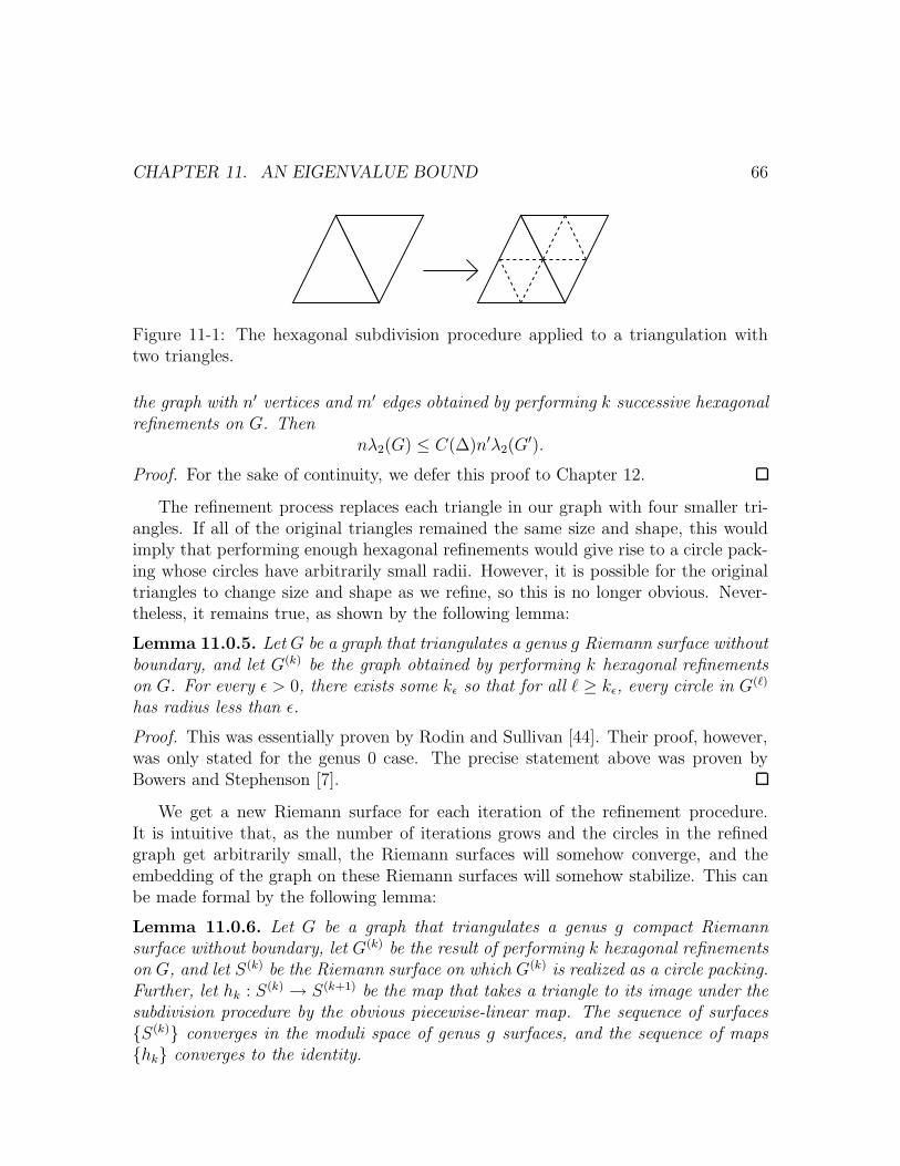
CHAPTER 11. AN EIGENVALUE BOUND 66
Figure 11-1: The hexagonal subdivision procedure applied to a triangulation withtwo triangles.
the graph with n′ vertices and m′ edges obtained by performing k successive hexagonalrefinements on G. Then
nλ2(G) ≤ C(∆)n′λ2(G′).
Proof. For the sake of continuity, we defer this proof to Chapter 12.
The refinement process replaces each triangle in our graph with four smaller tri-angles. If all of the original triangles remained the same size and shape, this wouldimply that performing enough hexagonal refinements would give rise to a circle pack-ing whose circles have arbitrarily small radii. However, it is possible for the originaltriangles to change size and shape as we refine, so this is no longer obvious. Never-theless, it remains true, as shown by the following lemma:
Lemma 11.0.5. Let G be a graph that triangulates a genus g Riemann surface withoutboundary, and let G(k) be the graph obtained by performing k hexagonal refinementson G. For every ε > 0, there exists some kε so that for all ` ≥ kε, every circle in G(`)
has radius less than ε.
Proof. This was essentially proven by Rodin and Sullivan [44]. Their proof, however,was only stated for the genus 0 case. The precise statement above was proven byBowers and Stephenson [7].
We get a new Riemann surface for each iteration of the refinement procedure.It is intuitive that, as the number of iterations grows and the circles in the refinedgraph get arbitrarily small, the Riemann surfaces will somehow converge, and theembedding of the graph on these Riemann surfaces will somehow stabilize. This canbe made formal by the following lemma:
Lemma 11.0.6. Let G be a graph that triangulates a genus g compact Riemannsurface without boundary, let G(k) be the result of performing k hexagonal refinementson G, and let S(k) be the Riemann surface on which G(k) is realized as a circle packing.Further, let hk : S(k) → S(k+1) be the map that takes a triangle to its image under thesubdivision procedure by the obvious piecewise-linear map. The sequence of surfacesS(k) converges in the moduli space of genus g surfaces, and the sequence of mapshk converges to the identity.
CHAPTER 11. AN EIGENVALUE BOUND 67
Proof. This is proven by Bowers and Stephenson [7].
We shall also require one last definition:
Definition 11.0.7. Let f : X → Y be a map between two locally Euclidean metricspaces. The quantity
Hf(x, r) =max|x−y|=r |f(x) − f(y)|min|x−y|=r |f(x) − f(y)| − 1.
is called the radius r distortion of f at x.
We are now finally ready to prove Theorem 8.1.3.Proof of Theorem 8.1.3. Using the Circle Packing Theorem (Theorem 10.3.2),
realize the graph G = G(0) as a circle packing on some Riemann surface S of genus g.Let G(k) be the result of performing k hexagonal refinements on G, and let S (k) be theRiemann surface on which it can be realized as a circle packing. By Theorem 10.2.2,there exists an analytic map f (k) from S(k) to the Riemann sphere of degree O(g) andwith O(g) branch points. Embed the Riemann sphere as the unit sphere in R3 usingthe conformal map given by inverse stereographic projection. By the work of Spielmanand Teng (Theorem 9 of [47]), post-composing with a Mobius transformation allowsus to assume, without loss of generality, that the centroid of the images of the verticesof each G(k) under f (k) is the origin. By Lemma 11.0.6, the S(k) converge to somesurface S(∞), and the f (k) can be chosen so as to converge to some continuous limitmap f (∞).
By Lemma 11.0.4, it suffices to the prove the theorem for an arbitrarily finehexagonal refinement of the original graph. Away from its branch points, a map ofRiemann surfaces is conformal, meaning it sends infinitesimal circles to infinitesimalcircles. In particular, given a map f : S → C, the compactness of S guarantees thatfor every ε, κ > 0, there exists a δ > 0 so that the radius δ ′ distortion Hf(x, δ′) is lessthan ε for every x that is at least distance κ from any branch point and any δ ′ ≤ δ.In fact, by the convergence results of the last paragraph, there exist some N and δsuch that this holds for every f (k) with k > N . Fix ε and κ, and let δ and N bechosen so that this is true. By possibly increasing N if necessary, we can assume byLemma 11.0.5 that all of the circles on S(k) have radius at most δ for all k > N .
Let k be at least N . We shall break S(k) into two parts, S(k) = S(k)1 ∪ S
(k)2 , as
follows. Construct a ball of radius κ around each branch point of f (k), and let S(k)2
be the union of these balls. Let S(k)1 be the complement S(k) − S
(k)2 .
We can now use equation (11.3) to bound λ2, just as in the proof of Theorem 11.0.3.Let G(k) have nk vertices. The denominator of equation (11.3) is equal to nk, so it
CHAPTER 11. AN EIGENVALUE BOUND 68
suffices to bound the numerator. We shall consider separately the circles containedentirely in S
(k)1 and those that intersect S
(k)2 .
We begin with the circles contained in S(k)1 . Every circle of the packing gets
mapped by f to some connected region on C, and there are at most O(g) such regions
covering any point of the sphere. Let C be a circle in S(k)1 , let D be the diameter
function, which takes a region to the length of the longest geodesic it contains, andlet A be the area function. Since the radius δ distortion of f inside of S
(k)1 is at most
ε, and the radius of C is at most δ, the ratio D2(f(C))/A(f(C)) is at most O(1 + ε).Using the same argument as in the proof of Theorem 11.0.3, the vertex at the centerof a circle C cannot contribute more than O(dD2(f(C))) to the sum, and the total
area of the regions from S(k)1 cannot exceed O(g), so the total contribution to the
numerator of the vertices in S(k)1 cannot be more than O(dg(1 + ε)).
If this were the only term in the numerator, we could complete the proof bysetting ε to be a constant. It thus remains to show that the contribution from thecircles intersecting S
(k)2 can be made small. To do this, we need only show that the
contribution θ(k)(x) to the numerator per unit area at a point x from these circles
remains bounded as we subdivide, since we can make the area of S(k)2 arbitrarily small
by sending κ to zero, and thus the area of the circles intersecting S(k)2 will go to zero
as k goes to infinity and the circles get arbitrarily small.Let xi, i = 1, . . . , 3, be the coordinate functions on R3, and let f (k)∗xi be their
pullbacks along f (k) to S(k). (That is, if y is a point on S(k), f (k)∗xi(y) = xi(f(k)(y)).)
In addition, let C(k)1 and C
(k)2 be a pair of adjacent circles in S
(k)2 with respective radii
r(k)1 and r
(k)2 and respective centers c
(k)1 and c
(k)2 . The contribution of the corresponding
edge in G(k) to the numerator of equation (11.3) will be
∥∥∥∥(f (k)∗xi(c
(k)1 ))3
i=1−(f (k)∗xi(c
(k)2 ))3
i=1
∥∥∥∥2
(11.4)
=
3∑
i=1
(f (k)∗xi(c
(k)1 ) − f (k)∗xi(c
(k)2 ))2
.
The distance between c(k)1 and c
(k)2 equals r
(k)1 + r
(k)2 . As k goes to infinity, the
radii r(k)1 and r
(k)2 both go to zero, by Lemma 11.0.5. By the smoothness of the f (k),
their convergence to f (∞), and the compactness of their domains, we can approximateeach term on the right-hand side of equation (11.4) arbitrarily well by its first order
CHAPTER 11. AN EIGENVALUE BOUND 69
approximation, so that
(f (k)∗xi(c
(k)1 ) − f (k)∗xi(c
(k)2 ))2
(11.5)
≤ (1 + o(1))(r(k)1 + r
(k)2 )2‖∇f (k)∗xi(c
(k)1 )‖2
as k goes to infinity and the distance between c(k)1 and c
(k)2 shrinks to zero.
The right-hand side of equation (11.5) is bounded above by
(2 + o(1))[(r(k)1 )2 + (r
(k)2 )2]‖∇f (k)∗xi(c
(k)1 )‖2 (11.6)
= O(1)[(r(k)1 )2‖∇f (k)∗xi(c
(k)1 )‖2 + (r
(k)2 )2‖∇f (k)∗xi(c
(k)2 )‖2].
The degree of our graph is bounded, so every vertex appears in at most a constantnumber of edges. If we sum the right-hand side of equation (11.6) over all of theedges in our graph, the total contribution of terms involving a fixed circle of radius rcentered at c is thus bounded above by
O(1)r2‖∇f (k)∗xi(c)‖2,
so the contribution per unit area is bounded above by
O(1)‖∇f (k)∗xi(c)‖2.
This clearly remains bounded as k goes to infinity and f (k) approaches f (∞). It thusfollows that the contribution to the numerator of equation (11.3) of the vertices in
S(k)2 tends to zero as k goes to infinity and κ is made arbitrarily small. By setting ε
to be a constant and sending κ to zero, Theorem 8.1.3 follows.
Chapter 12
The Proof of the Subdivision
Lemma
In this section, we shall prove Lemma 11.0.4. In proving this bound, it will beconvenient to consider a weighted form of the Laplacian:
Definition 12.0.8. The weighted Laplacian LW (G) of a graph G is the matrix
LW (G) = W−1/2L(G)W−1/2,
where L(G) is the Laplacian of G, and W is a diagonal matrix whose ith diagonalentry wi is strictly positive for all i.
We shall denote the eigenvalues of LW (G) by λW1 (G) ≤ · · · ≤ λW
n (G) and thecorresponding eigenvectors by vW
1 (G) . . . vWn (G). A straightforward calculation shows
that the weighted Laplacian has λW1 = 0 and vW
1 = W 1/21. Our main quantity
of interest will be λW2 (G), which we can compute using a weighted analogue of the
Rayleigh quotient:
λW2 = min
x⊥W1
∑(i,j)∈E(xi − xj)
2
∑i x
2i wi
. (12.1)
The second eigenvector vW2 (G) equals W 1/2x, where x is the vector that achieves the
minimum in equation (12.1).
If all of the weights are Θ(1), standard linear algebra shows that λ2(G) and λW2 (G)
differ by at most a constant factor, so proving a bound on one implies a bound onthe other. (See Chung’s book [12] for detailed proofs of the above facts and for otherfoundational information about the weighted Laplacian.)
Before we can proceed to the body of the proof of Lemma 11.0.4, we shall requiretwo fairly general technical lemmas about independent random variables.
70

CHAPTER 12. THE PROOF OF THE SUBDIVISION LEMMA 71
Lemma 12.0.9. Let a1, . . . , an be independent real-valued random variables, possiblydrawn from different probability distributions. Let w1, . . . , wn ∈ R+ be strictly positiveconstants. If the expectation E[
∑i wiai] = 0, then
E[(∑
j
wjaj
)2]≤ E
[∑
j
w2ja
2j
].
Proof. This follows by expanding out the left-hand side:
E[(∑
j
wjaj
)2]= E
[∑
i
w2i a
2i
]+ E
[∑
i
wiai
(∑
j 6=i
wjaj
)]
= E[∑
i
w2i a
2i
]+∑
i
−(E[wiai]
)2
≤ E[∑
j
w2ja
2j
],
where the second equality follows from the independence of the variables and the factthat the sum of their expectations is zero.
We shall now use this lemma to establish our second lemma, which is the one thatwill actually appear in our main proof:
Lemma 12.0.10. Let a1, . . . , an be independent real-valued random variables, possiblydrawn from different probability distributions, and let w1, . . . , wn ∈ R+ be strictlypositive constants such that E[
∑i wiai] = 0. Let a = (a1, . . . , an), and let wmax =
maxi wi. Further let
b =
(1∑i wi
∑
i
wiai
)1, and let c = a − b.
Then
E[∑
i
wic2i
]≥(
1 − wmax∑i wi
)E[∑
i
wia2i
].
CHAPTER 12. THE PROOF OF THE SUBDIVISION LEMMA 72
Proof. This follows by direct calculation:
E[∑
i
wic2i
]= E
[∑
i
wi
(ai −
1∑j wj
(∑
j
wjaj
))2]
= E[∑
i
wia2i
]+
1(∑
i wi
)2E[∑
i
wi
(∑
j
wjaj
)2]− 2∑i wi
E[∑
i
wiai
(∑
j
wjaj
)]
= E[∑
i
wia2i
]+
1∑i wi
E[(∑
j
wjaj
)2] − 2∑i wi
E[(∑
j
wjaj
)2]
= E[∑
i
wia2i
]− 1∑
i wiE[(∑
j
wjaj
)2]
≥ E[∑
i
wia2i
]− 1∑
i wiE[∑
j
w2ja
2j
]
= E[∑
i
(1 − wi∑
j wj
)wia
2i
]
≥(
1 − wmax∑i wi
)E[∑
i
wia2i
],
where second-to-last inequality follows from Lemma 12.0.9.
We are now prepared to prove Lemma 11.0.4.Proof of Lemma 11.0.4. Let G = (VG, EG) be the original graph, and let G′ =
(VG′, EG′) be the graph that results from performing k successive hexagonal refine-ments on G. The embeddings into surfaces endow both G and G′ with triangulations;let TG and TG′ be the respective sets of triangles in these triangulations. There is anatural inclusion ι : VG → VG′, since the subdivision procedure only adds vertices tothe original set. There is also a map η : TG′ → TG that takes a triangle from thesubdivided graph to the one in the original graph from which it arose. For a vertex vin either graph, let N(v) be the set of triangles containing it. For a vertex w ∈ VG, letP (w) = η−1(N(w)) be the set of triangles in T (G′) taken by η to elements of N(w).(See Figure 12-1.)
Our proof will proceed by producing a randomized construction of a subgraphH of G′. Given a vector that assigns a value to every vertex of G′, we can obtainsuch a vector on H by restriction. We shall also show how to use such a vector onH to construct such a vector on G. The vectors on the different graphs will giverise to Rayleigh quotients on the graphs (some of which will be weighted), wherethe Rayleigh quotients for G and H will depend on the random choices made in theconstruction of H. By relating the terms in the different Rayleigh quotients, we shall

CHAPTER 12. THE PROOF OF THE SUBDIVISION LEMMA 73
Figure 12-1: A subdivided graph, with P (w) and N(w) shaded for a vertex w.
then provide a probabilistic proof that there exists an H that gives rise to a smallRayleigh quotient on G, which will suffice to prove our desired bound.
H will be produced by randomly choosing a representative in VG′ for each vertexin VG and representing every edge in EG by a randomly chosen path in G′ betweenthe representatives of its endpoints.
We first construct the map πV : VG → VG′ that chooses the representatives of thevertices. For each v ∈ VG we choose πV (v) uniformly at random from the verticescontained in P (v) that are at least as close to ι(v) as to ι(w) for any other w ∈ VG.Vertices in P (v) that are equally close to ι(v) and ι(w) should be arbitrarily assignedto either v or w, but not both.
We now construct πE, which maps edges in EG to paths in G′. Let e = (v1, v2)be an edge in G, and let w1 and w2 equal πV (v1) and πV (v2) respectively. The twoneighborhoods in G, N(v1) and N(v2), share exactly two triangles, t1 and t2. Let xbe a vertex randomly chosen from the vertices in η−1(t1 ∪ t2). We shall construct apath from each wi (i = 1, 2) to x, so that their composition gives a path from w1 tow2. We shall use the same construction for each, so, without loss of generality, weshall just construct the path from w1 to x.
Both w1 and x are in P (v1), and we give a general procedure for constructing apath between any two such vertices. The images under the inclusion ι of the trianglesin N(v1) encircle ι(v1). Suppose w1 is contained in T1, and x is contained in T2.Traversing the triangles in a clockwise order from T1 to T2 gives one list of triangles,
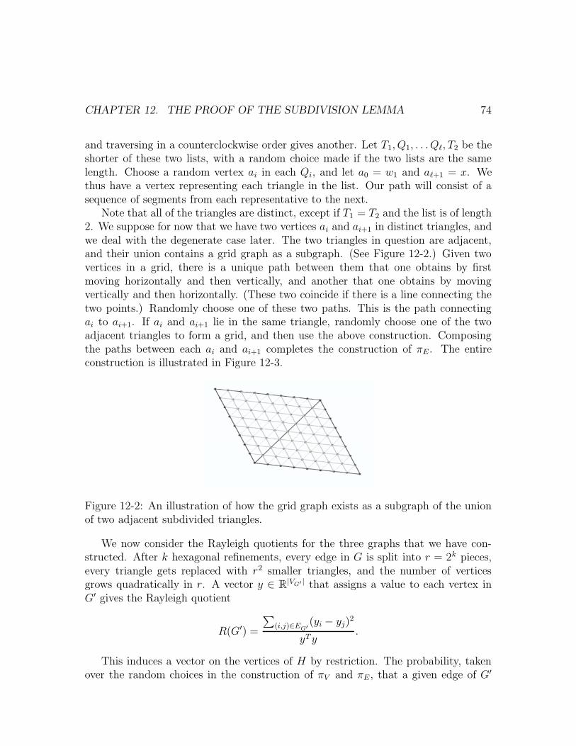
CHAPTER 12. THE PROOF OF THE SUBDIVISION LEMMA 74
and traversing in a counterclockwise order gives another. Let T1, Q1, . . . Q`, T2 be theshorter of these two lists, with a random choice made if the two lists are the samelength. Choose a random vertex ai in each Qi, and let a0 = w1 and a`+1 = x. Wethus have a vertex representing each triangle in the list. Our path will consist of asequence of segments from each representative to the next.
Note that all of the triangles are distinct, except if T1 = T2 and the list is of length2. We suppose for now that we have two vertices ai and ai+1 in distinct triangles, andwe deal with the degenerate case later. The two triangles in question are adjacent,and their union contains a grid graph as a subgraph. (See Figure 12-2.) Given twovertices in a grid, there is a unique path between them that one obtains by firstmoving horizontally and then vertically, and another that one obtains by movingvertically and then horizontally. (These two coincide if there is a line connecting thetwo points.) Randomly choose one of these two paths. This is the path connectingai to ai+1. If ai and ai+1 lie in the same triangle, randomly choose one of the twoadjacent triangles to form a grid, and then use the above construction. Composingthe paths between each ai and ai+1 completes the construction of πE. The entireconstruction is illustrated in Figure 12-3.
Figure 12-2: An illustration of how the grid graph exists as a subgraph of the unionof two adjacent subdivided triangles.
We now consider the Rayleigh quotients for the three graphs that we have con-structed. After k hexagonal refinements, every edge in G is split into r = 2k pieces,every triangle gets replaced with r2 smaller triangles, and the number of verticesgrows quadratically in r. A vector y ∈ R|VG′ | that assigns a value to each vertex inG′ gives the Rayleigh quotient
R(G′) =
∑(i,j)∈EG′
(yi − yj)2
yTy.
This induces a vector on the vertices of H by restriction. The probability, takenover the random choices in the construction of πV and πE, that a given edge of G′

CHAPTER 12. THE PROOF OF THE SUBDIVISION LEMMA 75
Figure 12-3: The entire construction illustrated for a given edge of the original graph.
CHAPTER 12. THE PROOF OF THE SUBDIVISION LEMMA 76
appears on the path representing a given edge e of G is zero if it is not in P (α)with α equal to one of the endpoints of e, and at most O(1/r) otherwise. Since themaximum degree of a vertex in G is assumed constant, the expected number of timesthat a given edge of G′ occurs in H is O(1/r). Every vertex in G′ is selected as arepresentative of a vertex in G with probability Θ(1/r2). It thus follows that
E
∑
(i,j)∈EH
(yi − yj)2
≤ O(1/r)
∑
(i,j)∈EG′
(yi − yj)2, (12.2)
and
E
[∑
i∈VG
wiy2πV (i)
]= Θ(1/r2)
∑
i∈VG′
y2i , (12.3)
where the expectations are taken over the random choices in the construction of(πV , πE), and the wi are any weights that are bounded above and below by positiveconstants.
Let y be the vector in R|VG| whose ith coordinate is yπV (i). Each coordinate yi ofy is chosen independently from a distinct set Si of the coordinates of y, and everycoordinate is contained in one of these sets. Let si = |Si|, let smin = mini si, andtake W to be the diagonal matrix whose ith diagonal entry wi equals si/smin. Theprobability that a given vertex in Si is selected equals 1/si, so we have that
E
[ ∑
j∈VG
wjyj
]=∑
k∈VG′
yk = 0.
(The necessity to weight the terms on the left-hand side of this expression by the wi
is what will necessitate the use of the weighted Laplacian in our proof.) The size ofeach Si is approximately proportional to the degree of the ith vertex of G, so the wi
are all bounded above by a constant, and they are all at least one by definition. Theeigenvalue λW
2 (G) of the weighted Laplacian is thus within a constant factor of thestandard Fiedler value λ2(G).
Let z be the vector
z = y −(∑
i wiyi∑i wi
)1,
so that z differs from y by a multiple of the all-ones vector and is orthogonal to W1.
CHAPTER 12. THE PROOF OF THE SUBDIVISION LEMMA 77
By applying Lemma 12.0.10 to equation (12.3), we obtain
E
[∑
i∈VG
wiz2i
]≥(
1 − wmax∑i wi
)E
[∑
i∈VG
wiy2i
]= Θ(1/r2)
∑
i∈VG′
y2i . (12.4)
Multiplying the inequalities in (12.2) and (12.4) by the appropriate factors and com-bining them yields
O(r)
∑
(i,j)∈EG′
(yi − yj)2
·E
[∑
i∈VG
wiz2i
]≥
∑
i∈VG′
y2i
·E
∑
(i,j)∈EH
(yi − yj)2
(12.5)
This implies that there exists some choice of (πV , πE) for which the left-hand sideof (12.5) is greater than or equal to the right-hand side, in which case we would have
∑(i,j)∈EH
(yi − yj)2
∑i∈VG
wiz2i
≤ O(r)
∑(i,j)∈EG′
(yi − yj)2
∑i∈VG′
y2i
= O(r)R(G′). (12.6)
Now suppose that we assign to each vertex v ∈ VG the value assumed by y atπV (v). Using the fact that maximum degree of a vertex is bounded, so that there areO(1) triangles surrounding any vertex in G, we see that every path representing anedge is of length O(r). We note that if i1, . . . , is is a sequence of vertices,
(yis − yi1)2 ≤ s
s−1∑
a=1
(yia+1 − yia)2.
As such, we have
∑
(i,j)∈EG
(yπV (i) − yπV (j))2 ≤ O(r)
∑
(i,j)∈EH
(yi − yj)2. (12.7)
Since z is obtained from y by subtracting a multiple of the all-ones vector,
zi − zj = yπV (i) − yπV (j)
for any i and j. Plugging this into equation (12.7) gives
∑
(i,j)∈EG
(zi − zj)2 ≤ O(r)
∑
(i,j)∈EH
(yi − yj)2,
CHAPTER 12. THE PROOF OF THE SUBDIVISION LEMMA 78
and applying this to the inequality in (12.6) yields
∑(i,j)∈EG
(zi − zj)2
∑i∈VG
wiz2i
≤ O(r2)R(G′).
We have thus constructed an assignment of values to the vertices of G that is or-thogonal to the vector W1 and produces a weighted Rayleigh quotient of O(r2)R(G′).If we choose the yi to be the values that give the Fiedler value of G′, we thus obtain,by equation (12.1) and the fact that the wi are Θ(1),
λ2(G) = Θ(1)λW2 (G) ≤ O(r2)λ2(G
′).
Since the number of vertices in G′ grows as r2 times the number of vertices in G, thiscompletes the proof of Lemma 11.0.4.

Bibliography
[1] Noga Alon, Paul Seymour, and Robin Thomas. A separator theorem for non-planar graphs. Journal of the American Mathematical Society, 3(4):801–808,October 1990.
[2] C. J. Alpert and A. B. Kahng. Recent directions in netlist partitioning: a survey.Integration: the VLSI Journal, 19:1–81, 1995.
[3] Alan F. Beardon and Kenneth Stephenson. The uniformization theorem for circlepackings. Indiana University Mathematics Journal, 39:1383–1425, 1990.
[4] Dimitris Bertsimas and Santosh Vempala. Solving convex programs by randomwalks. J. ACM, 51(4):540–556, 2004.
[5] T. Bonnesen and W. Fenchel. Theory of Convex Bodies. B C S Associates, 1988.
[6] Karl Heinz Borgwardt. The Simplex Method: a probabilistic analysis. Number 1in Algorithms and Combinatorics. Springer-Verlag, 1980.
[7] Philip Bowers and Kenneth Stephenson. Uniformizing dessinsand Belyi maps via circle packing. To appear. Available athttp://web.math.fsu.edu/~bowers/Papers/ recentPapers.html, 2003.
[8] P.K. Chan, M. Schlag, and J. Zien. Spectral k-way ratio cut partitioning andclustering. In Symposium on Integrated Systems, 1993.
[9] T.F. Chan and D. C. Resasco. A framework for the analysis and construction ofdomain decomposition preconditioners. Technical report, UCLA, 1987.
[10] T.F. Chan and B. Smith. Domain decomposition and multigrid algorithms forelliptic problems on unstructured meshes. Contemporary Mathematics, pages1–14, 1993.
[11] A. Charnes. Optimality and degeneracy in linear programming. Econometrica,20:160–170, 1952.
79
BIBLIOGRAPHY 80
[12] Fan R.K. Chung. Spectral Graph Theory. American Mathematical Society, 1997.
[13] Vasek Chvatal. Linear Programming. W.H. Freeman, 1983.
[14] G. B. Dantzig. Maximization of linear function of variables subject to linearinequalities. In T. C. Koopmans, editor, Activity Analysis of Production andAllocation, pages 339–347. 1951.
[15] G. B. Dantzig. Linear Programming and Extensions. Princeton University Press,1963.
[16] Amit Deshpande and Daniel A. Spielman. Improved smoothed analysis of theshadow vertex simplex method. preliminary version appeared in FOCS ’05, 2005.
[17] H. Djidjev and J. Reif. An efficient algorithm for the genus problem with explicitconstruction of forbidden subgraphs. In Proceedings of the 23rd Annual ACMSymposium on the Theory of Computing, pages 337–348, 1991.
[18] H.N. Djidjev. A linear algorithm for partitioning graphs. Comptes rendus del’Academie Bulgare des Sciences, 35:1053–1056, 1982.
[19] John Dunagan and Santosh Vempala. A simple polynomial-time rescaling algo-rithm for solving linear programs. In Proceedings of the thirty-sixth annual ACMSymposium on Theory of Computing (STOC-04), pages 315–320, New York, June13–15 2004. ACM Press.
[20] I.S. Filotti, G.L. Miller, and J.H. Reif. On determining the genus of a graphin O(vO(g)) steps. In Proceedings of the 11th Annual ACM Symposium on theTheory of Computing, pages 27–37, 1979.
[21] Otto Forster. Lectures on Riemann Surfaces. Springer-Verlag, 1981.
[22] K. Fukuda and T. Terlaky. Criss-cross methods: A fresh view on pivot algo-rithms. Mathematical Programming, 79:369–395, 1997.
[23] Bernd Gartner, Martin Henk, and Gunter Ziegler. Randomized simplex algo-rithms on Klee-Minty cubes. Combinatorica, 18:349–372, 1998.
[24] S. Gass and Th. Saaty. The computational algorithm for the parametric objectivefunction. Naval Research Logistics Quarterly, 2:39–45, 1955.
[25] J.R. Gilbert, J. Hutchinson, and R. Tarjan. A separation theorem for graphs ofbounded genus. Journal of Algorithms, 5:391–407, 1984.
BIBLIOGRAPHY 81
[26] Martin Grotschel, Laszlo Lovasz, and Alexander Schrijver. Geometric Algorithmsand Combinatorial Optimization. Springer-Verlag, 1991.
[27] S. Guattery and G.L. Miller. On the performance of the spectral graph parti-tioning methods. In Proceedings of the Second Annual ACM-SIAM Symposiumon Discrete Algorithms, pages 233–242, 1995.
[28] L. Hagen and A. B. Kahng. New spectral methods for ratio cut partitioningand clustering. IEEE Transactions on computer-aided design, 11(9):1074–1085,September 1992.
[29] Zheng-Xu He and Oded Schramm. Fixed points, Koebe uniformization and circlepackings. Annals of Mathematics, 137:369–406, 1993.
[30] G. Kalai. A subexponential randomized simplex algorithm. In Proc. 24th Ann.ACM Symp. on Theory of Computing, pages 475–482, Victoria, B.C., Canada,May 1992.
[31] Gil Kalai and Daniel J. Kleitman. A quasi-polynomial bound for the diameterof graphs of polyhedra. Bulletin Amer. Math. Soc., 26:315–316, 1992.
[32] N. Karmarkar. A new polynomial time algorithm for linear programming. Com-binatorica, 4:373–395, 1984.
[33] Jonathan A. Kelner. Spectral partitioning, eigenvalue bounds, and circle pack-ings for graphs of bounded genus. In Symposium on the Theory of Computation(STOC), 2004.
[34] Jonathan A. Kelner. Spectral partitioning, eigenvalue bounds, and circle pack-ings for graphs of bounded genus. Master’s thesis, Massachusetts Institute ofTechnology, 2005.
[35] Jonathan A. Kelner. Spectral partitioning, eigenvalue bounds, and circle pack-ings for graphs of bounded genus. SIAM Journal on Computing, Special Issuefor STOC 2004, 35(4), 2006.
[36] Jonathan A. Kelner and Evdokia Nikolova. On the hardness and smoothedcomplexity of quasi-concave minimization. To appear.
[37] Jonathan A. Kelner and Daniel A. Spielman. A randomized polynomial-timesimplex algorithm for linear programming. In Symposium on the Theory of Com-putation (STOC), 2006.

BIBLIOGRAPHY 82
[38] L. G. Khachiyan. A polynomial algorithm in linear programming. DokladyAkademia Nauk SSSR, pages 1093–1096, 1979.
[39] R. J. Lipton and R. E. Tarjan. A separator theorem for planar graphs. SIAMJournal of Applied Mathematics, 36:177–189, April 1979.
[40] N. Megiddo and R. Chandrasekaran. On the epsilon-perturbation method foravoiding degeneracy. Operations Research Letters, 8:305–308, 1989.
[41] G. Mihail. Conductance and convergence of markov chains—a combinatorialtreatment of expanders. In Proceedings of the 29th Annual IEEE Conference onFoundations of Computer Scienc, pages 526–531, 1989.
[42] Bojan Mohar. A linear time algorithm for embedding graphs in an arbitrarysurface. SIAM Journal of Discrete Mathematics, 12:6–26, 1999.
[43] Evdokia Nikolova, Jonathan A. Kelner, Matthew Brand, and Michael Mitzen-macher. Stochastic shortest paths via quasi-convex maximization. In Proceedingsof the European Symposium on Algorithms, 2006.
[44] Burt Rodin and Dennis Sullivan. The convergence of circle packings to theRiemann mapping. J. Differential Geometry, 26:349–360, 1987.
[45] A. Schrijver. Theory of Linear and Integer Programming. John Wiley & Sons,1986.
[46] H.D. Simon. Partitioning of unstructured problems for parallel processing. Com-puter Systems in Engineering, 2(2/3):135–148, 1991.
[47] Daniel A. Spielman and Shang-Hua Teng. Spectral partitioning works: Planargraphs and finite element meshes. In Proceedings of the 37th Annual IEEEConference on Foundations of Computer Science, 1996.
[48] Ken Stephenson. Circle packing and discrete analytic function theory. Availableonline at http://www.math.utk.edu/~kens.
[49] C. Thomassen. The graph genus problem is NP-complete. Journal of Algorithms,10(4):568–576, December 1989.
[50] Robert J. Vanderbei. Linear Programming: Foundations and Extensions.Springer, 2nd edition, 2001.
[51] R. D. Williams. Performance of dynamic load balancing algorithms for unstruc-tured mesh calculations. Technical report, California Institute of Technology,1990.
Related Documents