New Directions in Traffic Measurement and Accounting: Focusing on the Elephants, Ignoring the Mice CRISTIAN ESTAN and GEORGE VARGHESE University of California, San Diego Accurate network traffic measurement is required for accounting, bandwidth provisioning and detecting DoS attacks. These applications see the traffic as a collection of flows they need to measure. As link speeds and the number of flows increase, keeping a counter for each flow is too expensive (using SRAM) or slow (using DRAM). The current state-of-the-art methods (Cisco’s sampled NetFlow), which count periodically sampled packets are slow, inaccurate and resource- intensive. Previous work showed that at different granularities a small number of “heavy hitters” accounts for a large share of traffic. Our paper introduces a paradigm shift by concentrating the measurement process on large flows only—those above some threshold such as 0.1% of the link capacity. We propose two novel and scalable algorithms for identifying the large flows: sample and hold and multistage filters, which take a constant number of memory references per packet and use a small amount of memory. If M is the available memory, we show analytically that the errors of our new algorithms are proportional to 1/ M ; by contrast, the error of an algorithm based on classical sampling is proportional to 1/ √ M , thus providing much less accuracy for the same amount of memory. We also describe optimizations such as early removal and conservative update that further improve the accuracy of our algorithms, as measured on real traffic traces, by an order of magnitude. Our schemes allow a new form of accounting called threshold accounting in which only flows above a threshold are charged by usage while the rest are charged a fixed fee. Threshold accounting generalizes usage-based and duration based pricing. Categories and Subject Descriptors: C.2.3 [Computer-Communication Networks]: Network Operations—Network monitoring General Terms: Algorithms, Measurement Additional Key Words and Phrases: Network traffic measurement, usage based accounting, scala- bility, on-line algorithms, identifying large flows This work was made possible by a grant from NIST for the Sensilla Project, and by NSF Grant ANI 0074004. Authors’ address: Computer Science and Engineering Department, University of California, San Diego, 9500 Gillman Drive, La Jolla, CA 92093-0114; email: {cestan,varghese}@cs.ucsd.edu. Permission to make digital or hard copies of part or all of this work for personal or classroom use is granted without fee provided that copies are not made or distributed for profit or direct commercial advantage and that copies show this notice on the first page or initial screen of a display along with the full citation. Copyrights for components of this work owned by others than ACM must be honored. Abstracting with credit is permitted. To copy otherwise, to republish, to post on servers, to redistribute to lists, or to use any component of this work in other works requires prior specific permission and/or a fee. Permissions may be requested from Publications Dept., ACM, Inc., 1515 Broadway, New York, NY 10036 USA, fax: +1 (212) 869-0481, or [email protected]. C 2003 ACM 0734-2071/03/0800-0270 $5.00 ACM Transactions on Computer Systems, Vol. 21, No. 3, August 2003, Pages 270–313.

Welcome message from author
This document is posted to help you gain knowledge. Please leave a comment to let me know what you think about it! Share it to your friends and learn new things together.
Transcript
New Directions in Traffic Measurement andAccounting: Focusing on the Elephants,Ignoring the Mice
CRISTIAN ESTAN and GEORGE VARGHESEUniversity of California, San Diego
Accurate network traffic measurement is required for accounting, bandwidth provisioning anddetecting DoS attacks. These applications see the traffic as a collection of flows they need tomeasure. As link speeds and the number of flows increase, keeping a counter for each flow istoo expensive (using SRAM) or slow (using DRAM). The current state-of-the-art methods (Cisco’ssampled NetFlow), which count periodically sampled packets are slow, inaccurate and resource-intensive. Previous work showed that at different granularities a small number of “heavy hitters”accounts for a large share of traffic. Our paper introduces a paradigm shift by concentrating themeasurement process on large flows only—those above some threshold such as 0.1% of the linkcapacity.
We propose two novel and scalable algorithms for identifying the large flows: sample and holdand multistage filters, which take a constant number of memory references per packet and use asmall amount of memory. If M is the available memory, we show analytically that the errors of ournew algorithms are proportional to 1/M ; by contrast, the error of an algorithm based on classicalsampling is proportional to 1/
√M , thus providing much less accuracy for the same amount of
memory. We also describe optimizations such as early removal and conservative update that furtherimprove the accuracy of our algorithms, as measured on real traffic traces, by an order of magnitude.Our schemes allow a new form of accounting called threshold accounting in which only flows abovea threshold are charged by usage while the rest are charged a fixed fee. Threshold accountinggeneralizes usage-based and duration based pricing.
Categories and Subject Descriptors: C.2.3 [Computer-Communication Networks]: NetworkOperations—Network monitoring
General Terms: Algorithms, Measurement
Additional Key Words and Phrases: Network traffic measurement, usage based accounting, scala-bility, on-line algorithms, identifying large flows
This work was made possible by a grant from NIST for the Sensilla Project, and by NSF Grant ANI0074004.Authors’ address: Computer Science and Engineering Department, University of California, SanDiego, 9500 Gillman Drive, La Jolla, CA 92093-0114; email: {cestan,varghese}@cs.ucsd.edu.Permission to make digital or hard copies of part or all of this work for personal or classroom use isgranted without fee provided that copies are not made or distributed for profit or direct commercialadvantage and that copies show this notice on the first page or initial screen of a display alongwith the full citation. Copyrights for components of this work owned by others than ACM must behonored. Abstracting with credit is permitted. To copy otherwise, to republish, to post on servers,to redistribute to lists, or to use any component of this work in other works requires prior specificpermission and/or a fee. Permissions may be requested from Publications Dept., ACM, Inc., 1515Broadway, New York, NY 10036 USA, fax: +1 (212) 869-0481, or [email protected]© 2003 ACM 0734-2071/03/0800-0270 $5.00
ACM Transactions on Computer Systems, Vol. 21, No. 3, August 2003, Pages 270–313.
New Directions in Traffic Measurement and Accounting • 271
1. INTRODUCTION
If we’re keeping per-flow state, we have a scaling problem, and we’llbe tracking millions of ants to track a few elephants.—Van Jacobson,End-to-end Research meeting, June 2000.
Measuring and monitoring network traffic is required to manage today’scomplex Internet backbones [Feldmann et al. 2000; Duffield and Grossglauser2000]. Such measurement information is essential for short-term monitoring(e.g., detecting hot spots and denial-of-service attacks [Mahajan et al. 2001]),longer term traffic engineering (e.g., rerouting traffic [Shaikh et al. 1999] andupgrading selected links [Feldmann et al. 2000]), and accounting (e.g., to sup-port usage based pricing [Duffield et al. 2001]).
The standard approach advocated by the Real-Time Flow Measurement(RTFM) [Brownlee et al. 1999] Working Group of the IETF is to instrumentrouters to add flow meters at either all or selected input links. Today’s routers of-fer tools such as NetFlow [http://www.cisco.com/warp/public/732/Tech/netflow]that give flow level information about traffic.
The main problem with the flow measurement approach is its lack of scal-ability. Measurements on MCI traces as early as 1997 [Thomson et al. 1997]showed over 250,000 concurrent flows. More recent measurements in Fang andPeterson [1999] using a variety of traces show the number of flows betweenend host pairs in a one hour period to be as high as 1.7 million (Fix-West) and0.8 million (MCI). Even with aggregation, the number of flows in 1 hour in theFix-West used by Fang and Peterson [1999] was as large as 0.5 million.
It can be feasible for flow measurement devices to keep up with the in-creases in the number of flows (with or without aggregation) only if they usethe cheapest memories: DRAMs. Updating per-packet counters in DRAM isalready impossible with today’s line speeds; further, the gap between DRAMspeeds (improving 7–9% per year) and link speeds (improving 100% per year) isonly increasing. Cisco NetFlow, which keeps its flow counters in DRAM, solvesthis problem by sampling—only sampled packets result in updates. But Sam-pled NetFlow has problems of its own (as we show later) since sampling affectsmeasurement accuracy.
Despite the large number of flows, a common observation found in manymeasurement studies (e.g., Feldmann et al. [2000]; Fang and Peterson [1999])is that a small percentage of flows accounts for a large percentage of the traffic.Fang and Peterson [1999] show that 9% of the flows between AS pairs accountfor 90% of the byte traffic between all AS pairs.
For many applications, knowledge of these large flows is probably suffi-cient. Fang and Peterson [1999] and Pan et al. [2001] suggest achieving scalabledifferentiated services by providing selective treatment to only a small numberof large flows. Feldmann et al. [2000] underline the importance of knowledge of“heavy hitters” for decisions about network upgrades and peering. Duffield et al.[2001] propose a usage sensitive billing scheme that relies on exact knowledgeof the traffic of large flows but only samples of the traffic of small flows.
We conclude that it is infeasible to accurately measure all flows on high speedlinks, but many applications can benefit from accurately measuring only the
ACM Transactions on Computer Systems, Vol. 21, No. 3, August 2003.
272 • C. Estan and G. Varghese
few large flows. One can easily keep counters for a few large flows using a smallamount of fast memory (SRAM). However, how does the device know whichflows to track? If one keeps state for all flows to identify the few large flows, ourpurpose is defeated.
Thus a reasonable goal is to devise an algorithm that identifies large flowsusing memory that is only a small constant larger than is needed to describe thelarge flows in the first place. This is the central question addressed by this paper.We present two algorithms that provably identify large flows using such a smallamount of state. Further, our algorithms use only a few memory references perpacket, making them suitable for use in high speed routers. Our algorithmsproduce more accurate estimates than Sampled NetFlow, but they do processingand access memory for each packet. Therefore the small amount of memory theyuse has to be fast memory operating at line speeds.
1.1 Problem Definition
A flow is generically defined by an optional pattern (which defines which packetswe will focus on) and an identifier (values for a set of specified header fields). Wecan also generalize by allowing the identifier to be a function of the header fieldvalues (e.g., using prefixes instead of addresses based on a mapping using routetables). Flow definitions vary with applications: for example for a traffic matrixone could use a wildcard pattern and identifiers defined by distinct source anddestination network numbers. On the other hand, for identifying TCP denialof service attacks one could use a pattern that focuses on TCP packets and usethe destination IP address as a flow identifier. Note that we do not require thealgorithms to simultaneously support all these ways of aggregating packets intoflows. The algorithms know a priori which flow definition to use and they donot need to ensure that a posteriori analyses based on different flow definitionsare possible (as they are based on NetFlow data).
Large flows are defined as those that send more than a given threshold(say 0.1% of the link capacity) during a given measurement interval (1 second,1 minute or even 1 hour). The technical report version of this paper [Estan andVarghese 2002] gives alternative definitions and algorithms based on defininglarge flows via leaky bucket descriptors.
An ideal algorithm reports, at the end of the measurement interval, the flowIDs and sizes of all flows that exceeded the threshold. A less ideal algorithmcan fail in three ways: it can omit some large flows, it can wrongly add somesmall flows to the report, and it can give an inaccurate estimate of the traffic ofsome large flows. We call the large flows that evade detection false negatives,and the small flows that are wrongly included false positives.
The minimum amount of memory required by an ideal algorithm is theinverse of the threshold; for example, there can be at most 1000 flows thatuse more than 0.1% of the link. We will measure the performance of analgorithm by four metrics: first, its memory compared to that of an ideal al-gorithm; second, the algorithm’s probability of false negatives; third, the algo-rithm’s probability of false positives; and fourth, the expected error in trafficestimates.
ACM Transactions on Computer Systems, Vol. 21, No. 3, August 2003.
New Directions in Traffic Measurement and Accounting • 273
1.2 Motivation
Our algorithms for identifying large flows can potentially be used to solve manyproblems. Since different applications define flows by different header fields,we need a separate instance of our algorithms for each of them. Applicationswe envisage include:
—Scalable Threshold Accounting: The two poles of pricing for network traf-fic are usage based (e.g., a price per byte for each flow) or duration based(e.g., a fixed price based on duration). While usage-based pricing [Mackie-Masson and Varian 1995; Shenker et al. 1996] has been shown to improveoverall utility, in its most complete form it is not scalable because we can-not track all flows at high speeds. We suggest, instead, a scheme where wemeasure all aggregates that are above z% of the link; such traffic is sub-ject to usage based pricing, while the remaining traffic is subject to durationbased pricing. By varying z from 0 to 100, we can move from usage basedpricing to duration based pricing. More importantly, for reasonably smallvalues of z (say 1%) threshold accounting may offer a compromise that isscalable and yet offers almost the same utility as usage based pricing. Alt-man and Chu [2001] offer experimental evidence based on the INDEX ex-periment that such threshold pricing could be attractive to both users andISPs.1
—Real-time Traffic Monitoring: Many ISPs monitor backbones for hot-spots in order to identify large traffic aggregates that can be rerouted (usingMPLS tunnels or routes through optical switches) to reduce congestion. Also,ISPs may consider sudden increases in the traffic sent to certain destinations(the victims) to indicate an ongoing attack. Mahajan et al. [2001] propose amechanism that reacts as soon as attacks are detected, but does not give amechanism to detect ongoing attacks. For both traffic monitoring and attackdetection, it may suffice to focus on large flows.
—Scalable Queue Management: At a smaller time scale, scheduling mecha-nisms seeking to approximate max-min fairness need to detect and penalizeflows sending above their fair rate. Keeping per flow state only for these flows[Feng et al. 2001; Pan et al. 2001] can improve fairness with small memory.We do not address this application further, except to note that our techniquesmay be useful for such problems. For example, Pan et al. [2001] use classicalsampling techniques to estimate the sending rates of large flows. Given thatour algorithms have better accuracy than classical sampling, it may be possi-ble to provide increased fairness for the same amount of memory by applyingour algorithms.
The rest of the paper is organized as follows. We describe related work inSection 2, describe our main ideas in Section 3, and provide a theoretical anal-ysis in Section 4. We theoretically compare our algorithms with NetFlow inSection 5. After showing how to dimension our algorithms in Section 6, we
1Besides Altman and Chu [2001], a brief reference to a similar idea can be found in Shenker et al.[1996]. However, neither paper proposes a fast mechanism to implement the idea.
ACM Transactions on Computer Systems, Vol. 21, No. 3, August 2003.
274 • C. Estan and G. Varghese
describe experimental evaluation on traces in Section 7. We end with imple-mentation issues in Section 8 and conclusions in Section 9.
2. RELATED WORK
The primary tool used for flow level measurement by IP backbone operators isCisco NetFlow. NetFlow keeps per flow counters in a large, slow DRAM. BasicNetFlow has two problems: i) Processing Overhead: updating the DRAMslows down the forwarding rate; ii) Collection Overhead: the amount of datagenerated by NetFlow can overwhelm the collection server or its network con-nection. For example Feldmann et al. [2000] report loss rates of up to 90% usingbasic NetFlow.
The processing overhead can be alleviated using sampling: per-flow coun-ters are incremented only for sampled packets.2 Classical random samplingintroduces considerable inaccuracy in the estimate; this is not a problem formeasurements over long periods (errors average out) and if applications do notneed exact data. However, we will show that sampling does not work well forapplications that require true lower bounds on customer traffic (e.g., it may beinfeasible to charge customers based on estimates that are larger than actualusage) and for applications that require accurate data at small time scales (e.g.,billing systems that charge higher during congested periods).
The data collection overhead can be alleviated by having the router aggregateflows (e.g., by source and destination AS numbers) as directed by a manager.However, Fang and Peterson [1999] show that even the number of aggregatedflows is very large. For example, collecting packet headers for Code Red traf-fic on a class A network [Moore 2001] produced 0.5 Gbytes per hour of com-pressed NetFlow data and aggregation reduced this data only by a factor of 4.Techniques described in Duffield et al. [2001] can be used to reduce the collec-tion overhead at the cost of further errors. However, it can considerably simplifyrouter processing to only keep track of heavy-hitters (as in our paper) if that iswhat the application needs.
Many papers address the problem of mapping the traffic of large IP net-works. Feldmann et al. [2000] deal with correlating measurements taken atvarious points to find spatial traffic distributions; the techniques in our papercan be used to complement their methods. Duffield and Grossglauser [2000]describe a mechanism for identifying packet trajectories in the backbone, thatis not focused towards estimating the traffic between various networks. Shaikhet al. [1999] propose that edge routers identify large long lived flows and routethem along less loaded paths to achieve stable load balancing. Our algorithmsmight allow the detection of these candidates for rerouting in higher speedrouters too.
Bloom filters [Bloom 1970] and stochastic fair blue [Feng et al. 2001] use sim-ilar but different techniques to our parallel multistage filters to compute verydifferent metrics (set membership and drop probability). In Tong and Reddy[1999] and Smitha et al. [2001] the authors look at various mechanisms for
2NetFlow preforms 1 in N periodic sampling, but to simplify the analysis we assume in this paperthat it performs ordinary sampling processing each packet with probability 1/N independently.
ACM Transactions on Computer Systems, Vol. 21, No. 3, August 2003.
New Directions in Traffic Measurement and Accounting • 275
identifying the high rate flows to ensure quality of service. Their algorithmsrely on caching flow identifiers and while some of their techniques are similarto our sampling technique and to what we call preserving entries, their algo-rithms as a whole are quite different from ours. Gibbons and Matias [1998]consider synopsis data structures that use small amounts of memory to ap-proximately summarize large databases, but their algorithms have also beenused for profiling program execution [Burrows et al. 2000]. Their counting sam-ples use the same core idea as our sample and hold algorithm. However, sincethe constraints and requirements in their setting (data warehouses updatedconstantly) are different from ours, the two final algorithms also differ. For ex-ample we need to take into account packet lengths, we operate over a sequenceof measurement intervals, and our algorithms need to ensure low worst perpacket processing times as opposed to amortized processing in the data ware-house context. Fang et al. [1998] look at efficient ways of answering icebergqueries, or counting the number of appearances of popular items in a database.Their multi-stage algorithm is similar to multistage filters that we propose.However, they use sampling as a front end before the filter and use multiplepasses. Thus their final algorithms and analyses are very different from ours.For instance, their analysis is limited to Zipf distributions while our’s holds forall traffic distributions. Cohen and Matias [2003] independently discovered inthe context of spectral Bloom filters the optimization to multistage filters wecall conservative upsate. Karp et al. [2003] give an algorithm that is guaran-teed to identify all elements that repeat frequently in a single pass. They usea second pass over the data to count exactly the number of occurrences of thefrequent elements because the first pass does not guarantee accurate results.Building on our work, Narayanasamy et al. [2003] use multistage filters withconservative update to determine execution profiles in hardware and obtainpromising results.
3. OUR SOLUTION
Because our algorithms use an amount of memory that is a constant factorlarger than the (relatively small) number of large flows, our algorithms can beimplemented using on-chip or off-chip SRAM to store flow state. We assumethat at each packet arrival we can afford to look up a flow ID in the SRAM,update the counter(s) in the entry or allocate a new entry if there is no entryassociated with the current packet.
The biggest problem is to identify the large flows. Two approaches suggestthemselves. First, when a packet arrives with a flow ID not in the flow memory,we could make place for the new flow by evicting the flow with the smallestmeasured traffic (i.e., smallest counter). While this works well on traces, itis possible to provide counter examples where a large flow is not measuredbecause it keeps being expelled from the flow memory before its counter becomeslarge enough. This can happen even when using an LRU replacement policy asin Smitha et al. [2001].
A second approach is to use classical random sampling. Random sampling(similar to sampled NetFlow except using a smaller amount of SRAM) provably
ACM Transactions on Computer Systems, Vol. 21, No. 3, August 2003.
276 • C. Estan and G. Varghese
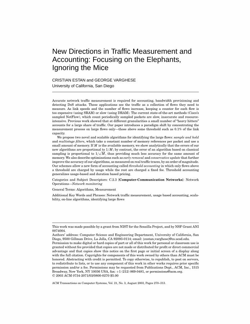
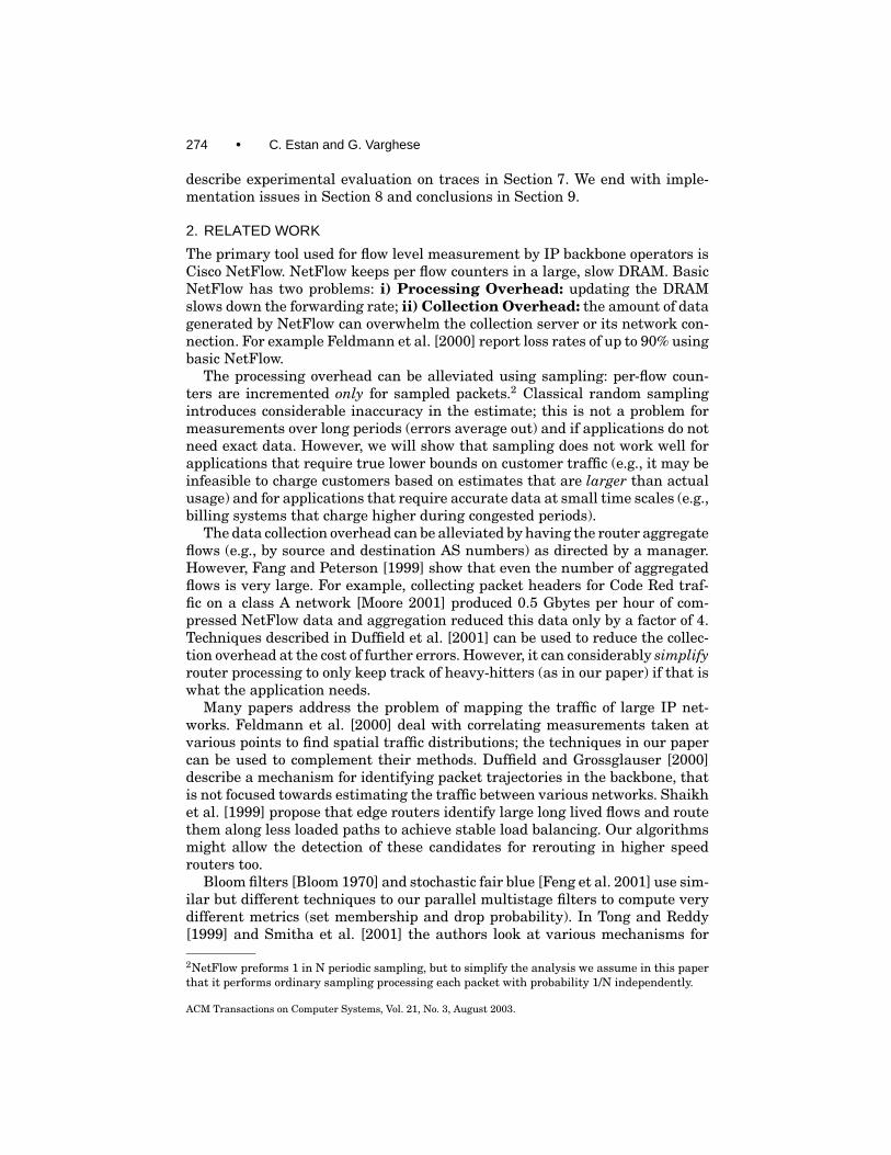
Fig. 1. The leftmost packet with flow label F1 arrives first at the router. After an entry is createdfor a flow (solid line) the counter is updated for all its packets (dotted lines).
identifies large flows. However, as the well known result from Table I (seepage 288) shows, random sampling introduces a very high relative error inthe measurement estimate, proportional to 1/
√M , where M is the amount of
SRAM used by the device. Thus one needs very high amounts of memory toreduce the inaccuracy to acceptable levels.
The two most important contributions of this paper are two new algorithmsfor identifying large flows: Sample and Hold (Section 3.1) and Multistage Filters(Section 3.2). Their performance is very similar, the main advantage of sampleand hold being implementation simplicity, and the main advantage of multi-stage filters being higher accuracy. In contrast to random sampling, the relativeerrors of our two new algorithms scale with 1/M , where M is the amount ofSRAM. This allows our algorithms to provide much more accurate estimatesthan random sampling using the same amount of memory. However, unlikesampled NetFlow, our algorithms access the memory for each packet, so theymust use memories fast enough to keep up with line speeds. In Section 3.3 wepresent improvements that further increase the accuracy of these algorithms ontraces (Section 7). We start by describing the main ideas behind these schemes.
3.1 Sample and Hold
Base Idea: The simplest way to identify large flows is through sampling butwith the following twist. As with ordinary sampling, we sample each packetwith a probability. If a packet is sampled and the flow it belongs to has noentry in the flow memory, a new entry is created. However, after an entry iscreated for a flow, unlike in sampled NetFlow, we update the entry for everysubsequent packet belonging to the flow as shown in Figure 1. The countingsamples of Gibbons and Matias [1998] use the same core idea.
Thus once a flow is sampled, a corresponding counter is held in a hash tablein flow memory till the end of the measurement interval. While this clearlyrequires processing (looking up the flow entry and updating a counter) for ev-ery packet (unlike Sampled NetFlow), we will show that the reduced memoryrequirements allow the flow memory to be in SRAM instead of DRAM. This inturn allows the per-packet processing to scale with line speeds.
ACM Transactions on Computer Systems, Vol. 21, No. 3, August 2003.
New Directions in Traffic Measurement and Accounting • 277
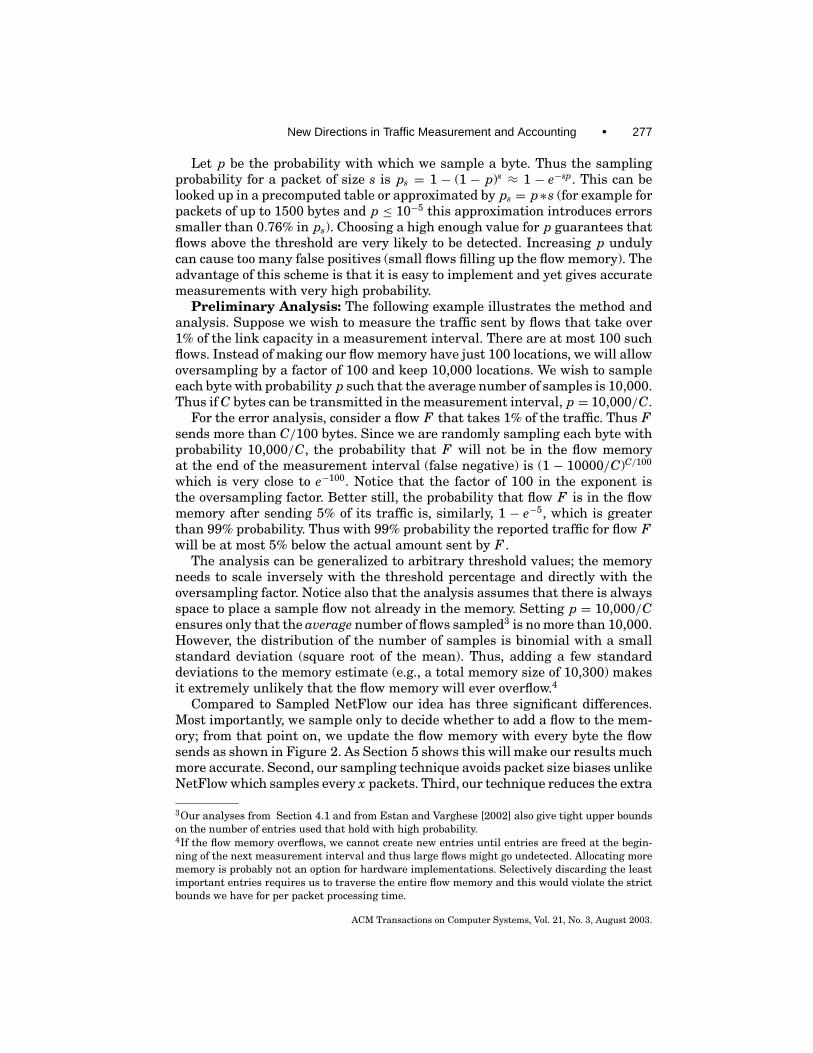
Let p be the probability with which we sample a byte. Thus the samplingprobability for a packet of size s is ps = 1 − (1 − p)s ≈ 1 − e−sp. This can belooked up in a precomputed table or approximated by ps = p∗s (for example forpackets of up to 1500 bytes and p ≤ 10−5 this approximation introduces errorssmaller than 0.76% in ps). Choosing a high enough value for p guarantees thatflows above the threshold are very likely to be detected. Increasing p undulycan cause too many false positives (small flows filling up the flow memory). Theadvantage of this scheme is that it is easy to implement and yet gives accuratemeasurements with very high probability.
Preliminary Analysis: The following example illustrates the method andanalysis. Suppose we wish to measure the traffic sent by flows that take over1% of the link capacity in a measurement interval. There are at most 100 suchflows. Instead of making our flow memory have just 100 locations, we will allowoversampling by a factor of 100 and keep 10,000 locations. We wish to sampleeach byte with probability p such that the average number of samples is 10,000.Thus if C bytes can be transmitted in the measurement interval, p = 10,000/C.
For the error analysis, consider a flow F that takes 1% of the traffic. Thus Fsends more than C/100 bytes. Since we are randomly sampling each byte withprobability 10,000/C, the probability that F will not be in the flow memoryat the end of the measurement interval (false negative) is (1 − 10000/C)C/100
which is very close to e−100. Notice that the factor of 100 in the exponent isthe oversampling factor. Better still, the probability that flow F is in the flowmemory after sending 5% of its traffic is, similarly, 1 − e−5, which is greaterthan 99% probability. Thus with 99% probability the reported traffic for flow Fwill be at most 5% below the actual amount sent by F .
The analysis can be generalized to arbitrary threshold values; the memoryneeds to scale inversely with the threshold percentage and directly with theoversampling factor. Notice also that the analysis assumes that there is alwaysspace to place a sample flow not already in the memory. Setting p = 10,000/Censures only that the average number of flows sampled3 is no more than 10,000.However, the distribution of the number of samples is binomial with a smallstandard deviation (square root of the mean). Thus, adding a few standarddeviations to the memory estimate (e.g., a total memory size of 10,300) makesit extremely unlikely that the flow memory will ever overflow.4
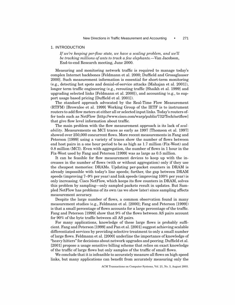
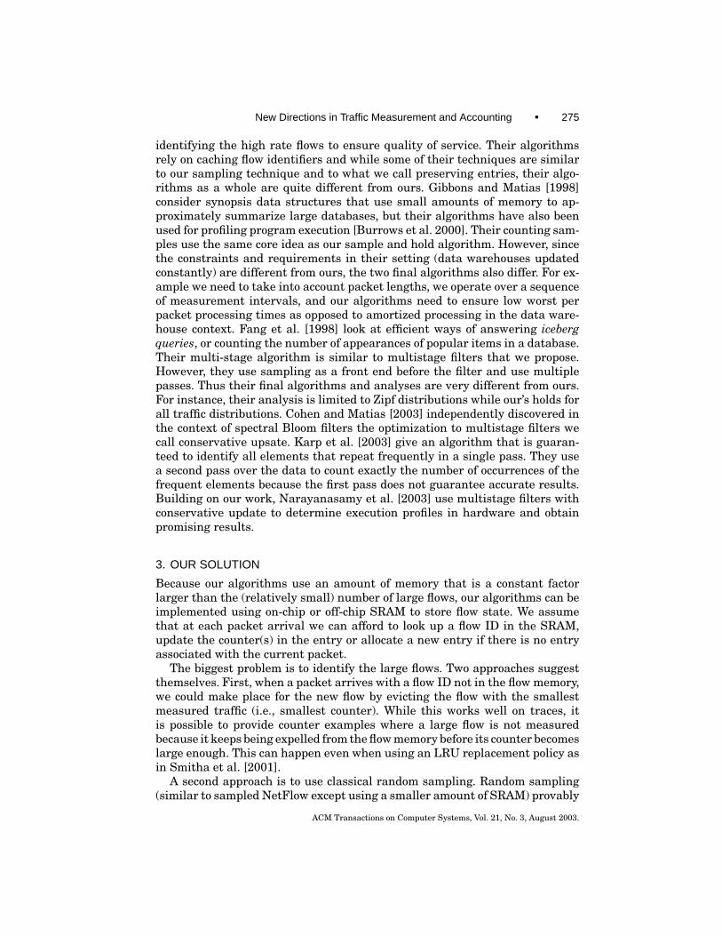
Compared to Sampled NetFlow our idea has three significant differences.Most importantly, we sample only to decide whether to add a flow to the mem-ory; from that point on, we update the flow memory with every byte the flowsends as shown in Figure 2. As Section 5 shows this will make our results muchmore accurate. Second, our sampling technique avoids packet size biases unlikeNetFlow which samples every x packets. Third, our technique reduces the extra
3Our analyses from Section 4.1 and from Estan and Varghese [2002] also give tight upper boundson the number of entries used that hold with high probability.4If the flow memory overflows, we cannot create new entries until entries are freed at the begin-ning of the next measurement interval and thus large flows might go undetected. Allocating morememory is probably not an option for hardware implementations. Selectively discarding the leastimportant entries requires us to traverse the entire flow memory and this would violate the strictbounds we have for per packet processing time.
ACM Transactions on Computer Systems, Vol. 21, No. 3, August 2003.
278 • C. Estan and G. Varghese
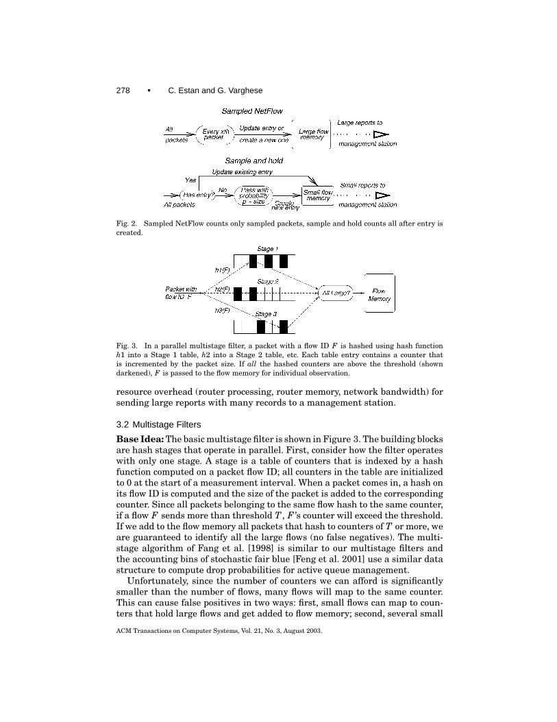
Fig. 2. Sampled NetFlow counts only sampled packets, sample and hold counts all after entry iscreated.
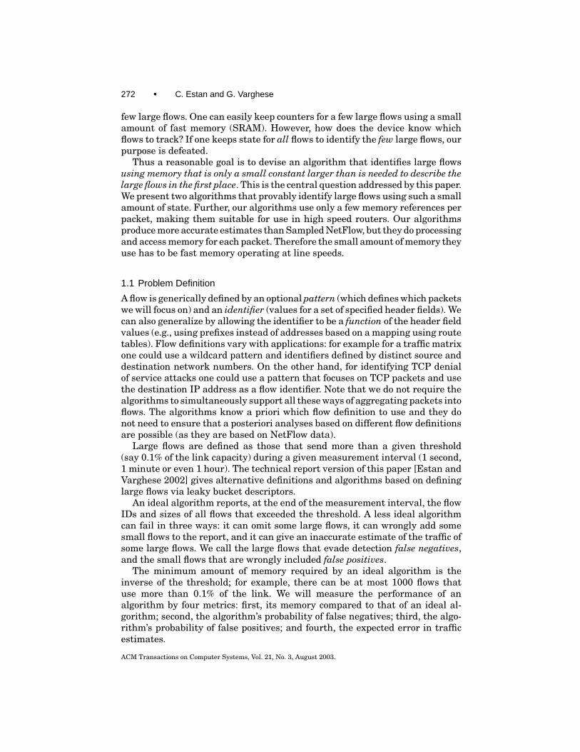
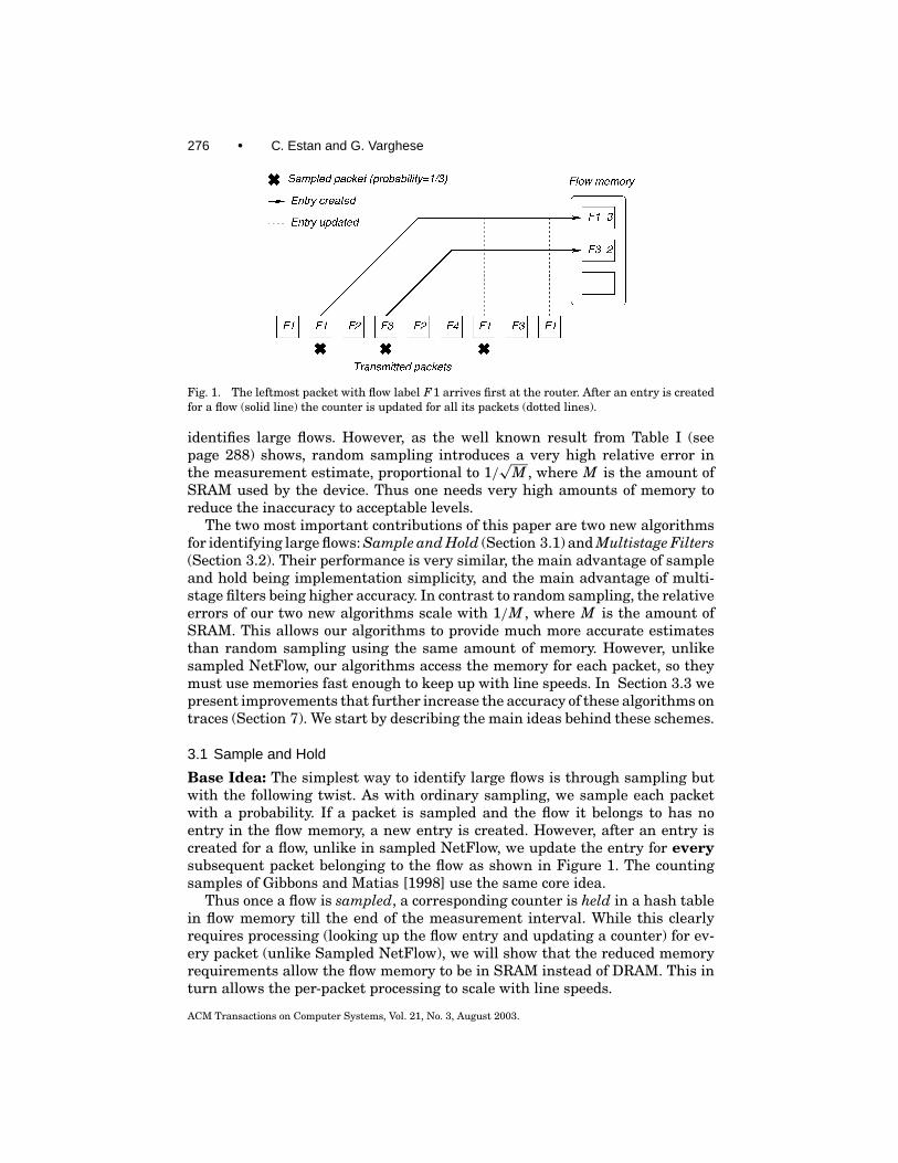
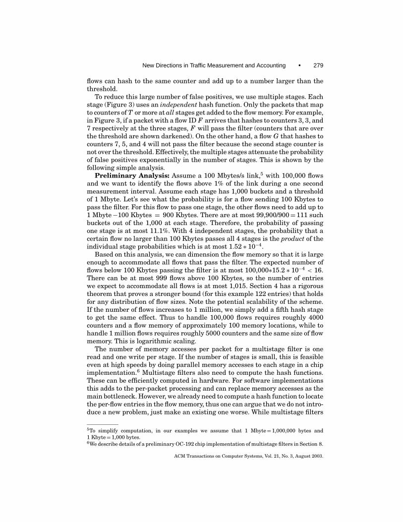
Fig. 3. In a parallel multistage filter, a packet with a flow ID F is hashed using hash functionh1 into a Stage 1 table, h2 into a Stage 2 table, etc. Each table entry contains a counter thatis incremented by the packet size. If all the hashed counters are above the threshold (showndarkened), F is passed to the flow memory for individual observation.
resource overhead (router processing, router memory, network bandwidth) forsending large reports with many records to a management station.
3.2 Multistage Filters
Base Idea: The basic multistage filter is shown in Figure 3. The building blocksare hash stages that operate in parallel. First, consider how the filter operateswith only one stage. A stage is a table of counters that is indexed by a hashfunction computed on a packet flow ID; all counters in the table are initializedto 0 at the start of a measurement interval. When a packet comes in, a hash onits flow ID is computed and the size of the packet is added to the correspondingcounter. Since all packets belonging to the same flow hash to the same counter,if a flow F sends more than threshold T , F ’s counter will exceed the threshold.If we add to the flow memory all packets that hash to counters of T or more, weare guaranteed to identify all the large flows (no false negatives). The multi-stage algorithm of Fang et al. [1998] is similar to our multistage filters andthe accounting bins of stochastic fair blue [Feng et al. 2001] use a similar datastructure to compute drop probabilities for active queue management.
Unfortunately, since the number of counters we can afford is significantlysmaller than the number of flows, many flows will map to the same counter.This can cause false positives in two ways: first, small flows can map to coun-ters that hold large flows and get added to flow memory; second, several small
ACM Transactions on Computer Systems, Vol. 21, No. 3, August 2003.
New Directions in Traffic Measurement and Accounting • 279
flows can hash to the same counter and add up to a number larger than thethreshold.
To reduce this large number of false positives, we use multiple stages. Eachstage (Figure 3) uses an independent hash function. Only the packets that mapto counters of T or more at all stages get added to the flow memory. For example,in Figure 3, if a packet with a flow ID F arrives that hashes to counters 3, 3, and7 respectively at the three stages, F will pass the filter (counters that are overthe threshold are shown darkened). On the other hand, a flow G that hashes tocounters 7, 5, and 4 will not pass the filter because the second stage counter isnot over the threshold. Effectively, the multiple stages attenuate the probabilityof false positives exponentially in the number of stages. This is shown by thefollowing simple analysis.
Preliminary Analysis: Assume a 100 Mbytes/s link,5 with 100,000 flowsand we want to identify the flows above 1% of the link during a one secondmeasurement interval. Assume each stage has 1,000 buckets and a thresholdof 1 Mbyte. Let’s see what the probability is for a flow sending 100 Kbytes topass the filter. For this flow to pass one stage, the other flows need to add up to1 Mbyte−100 Kbytes = 900 Kbytes. There are at most 99,900/900= 111 suchbuckets out of the 1,000 at each stage. Therefore, the probability of passingone stage is at most 11.1%. With 4 independent stages, the probability that acertain flow no larger than 100 Kbytes passes all 4 stages is the product of theindividual stage probabilities which is at most 1.52 ∗ 10−4.
Based on this analysis, we can dimension the flow memory so that it is largeenough to accommodate all flows that pass the filter. The expected number offlows below 100 Kbytes passing the filter is at most 100,000∗15.2 ∗ 10−4 < 16.There can be at most 999 flows above 100 Kbytes, so the number of entrieswe expect to accommodate all flows is at most 1,015. Section 4 has a rigoroustheorem that proves a stronger bound (for this example 122 entries) that holdsfor any distribution of flow sizes. Note the potential scalability of the scheme.If the number of flows increases to 1 million, we simply add a fifth hash stageto get the same effect. Thus to handle 100,000 flows requires roughly 4000counters and a flow memory of approximately 100 memory locations, while tohandle 1 million flows requires roughly 5000 counters and the same size of flowmemory. This is logarithmic scaling.
The number of memory accesses per packet for a multistage filter is oneread and one write per stage. If the number of stages is small, this is feasibleeven at high speeds by doing parallel memory accesses to each stage in a chipimplementation.6 Multistage filters also need to compute the hash functions.These can be efficiently computed in hardware. For software implementationsthis adds to the per-packet processing and can replace memory accesses as themain bottleneck. However, we already need to compute a hash function to locatethe per-flow entries in the flow memory, thus one can argue that we do not intro-duce a new problem, just make an existing one worse. While multistage filters
5To simplify computation, in our examples we assume that 1 Mbyte= 1,000,000 bytes and1 Kbyte= 1,000 bytes.6We describe details of a preliminary OC-192 chip implementation of multistage filters in Section 8.
ACM Transactions on Computer Systems, Vol. 21, No. 3, August 2003.
280 • C. Estan and G. Varghese
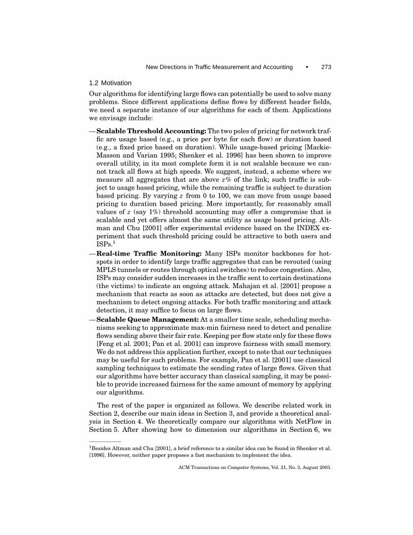
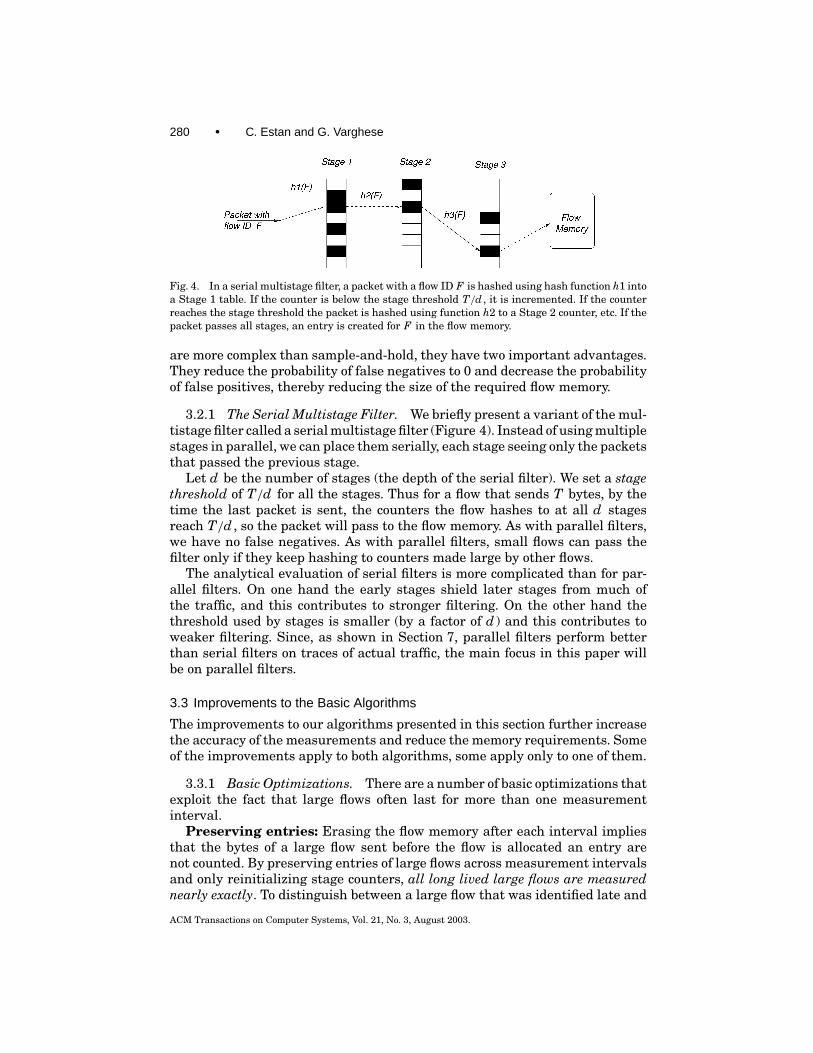
Fig. 4. In a serial multistage filter, a packet with a flow ID F is hashed using hash function h1 intoa Stage 1 table. If the counter is below the stage threshold T/d , it is incremented. If the counterreaches the stage threshold the packet is hashed using function h2 to a Stage 2 counter, etc. If thepacket passes all stages, an entry is created for F in the flow memory.
are more complex than sample-and-hold, they have two important advantages.They reduce the probability of false negatives to 0 and decrease the probabilityof false positives, thereby reducing the size of the required flow memory.
3.2.1 The Serial Multistage Filter. We briefly present a variant of the mul-tistage filter called a serial multistage filter (Figure 4). Instead of using multiplestages in parallel, we can place them serially, each stage seeing only the packetsthat passed the previous stage.
Let d be the number of stages (the depth of the serial filter). We set a stagethreshold of T/d for all the stages. Thus for a flow that sends T bytes, by thetime the last packet is sent, the counters the flow hashes to at all d stagesreach T/d , so the packet will pass to the flow memory. As with parallel filters,we have no false negatives. As with parallel filters, small flows can pass thefilter only if they keep hashing to counters made large by other flows.
The analytical evaluation of serial filters is more complicated than for par-allel filters. On one hand the early stages shield later stages from much ofthe traffic, and this contributes to stronger filtering. On the other hand thethreshold used by stages is smaller (by a factor of d ) and this contributes toweaker filtering. Since, as shown in Section 7, parallel filters perform betterthan serial filters on traces of actual traffic, the main focus in this paper willbe on parallel filters.
3.3 Improvements to the Basic Algorithms
The improvements to our algorithms presented in this section further increasethe accuracy of the measurements and reduce the memory requirements. Someof the improvements apply to both algorithms, some apply only to one of them.
3.3.1 Basic Optimizations. There are a number of basic optimizations thatexploit the fact that large flows often last for more than one measurementinterval.
Preserving entries: Erasing the flow memory after each interval impliesthat the bytes of a large flow sent before the flow is allocated an entry arenot counted. By preserving entries of large flows across measurement intervalsand only reinitializing stage counters, all long lived large flows are measurednearly exactly. To distinguish between a large flow that was identified late and
ACM Transactions on Computer Systems, Vol. 21, No. 3, August 2003.
New Directions in Traffic Measurement and Accounting • 281
a small flow that was identified by error, a conservative solution is to preservethe entries of not only the flows for which we count at least T bytes in thecurrent interval, but also all the flows that were added in the current interval(since they may be large flows that entered late).
Early removal: Sample and hold has a larger rate of false positives thanmultistage filters. If we keep for one more interval all the flows that obtaineda new entry, many small flows will keep their entries for two intervals. We canimprove the situation by selectively removing some of the flow entries createdin the current interval. The new rule for preserving entries is as follows. Wedefine an early removal threshold R that is less then the threshold T . At theend of the measurement interval, we keep all entries whose counter is at leastT and all entries that have been added during the current interval and whosecounter is at least R.
Shielding: Consider large, long lived flows that go through the filter eachmeasurement interval. Each measurement interval, the counters they hashto exceed the threshold. With shielding, traffic belonging to flows that havean entry in flow memory no longer passes through the filter (the counters inthe filter are not incremented for packets with an entry), thereby reducingfalse positives. If we shield the filter from a large flow, many of the counters ithashes to will not reach the threshold after the first interval. This reduces theprobability that a random small flow will pass the filter by hashing to countersthat are large because of other flows.
3.3.2 Conservative Update of Counters. We now describe an important op-timization for multistage filters that improves performance by an order of mag-nitude. Conservative update reduces the number of false positives of multistagefilters by three subtle changes to the rules for updating counters. In essence,we endeavour to increment counters as little as possible (thereby reducing falsepositives by preventing small flows from passing the filter) while still avoidingfalse negatives (i.e., we need to ensure that all flows that reach the thresholdstill pass the filter.)
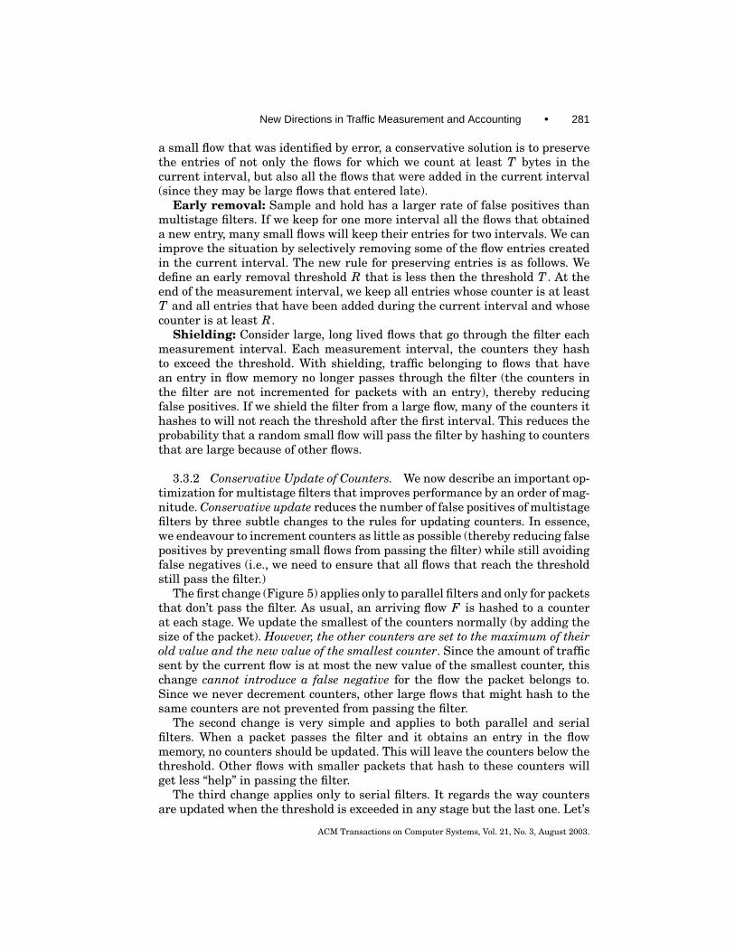
The first change (Figure 5) applies only to parallel filters and only for packetsthat don’t pass the filter. As usual, an arriving flow F is hashed to a counterat each stage. We update the smallest of the counters normally (by adding thesize of the packet). However, the other counters are set to the maximum of theirold value and the new value of the smallest counter. Since the amount of trafficsent by the current flow is at most the new value of the smallest counter, thischange cannot introduce a false negative for the flow the packet belongs to.Since we never decrement counters, other large flows that might hash to thesame counters are not prevented from passing the filter.
The second change is very simple and applies to both parallel and serialfilters. When a packet passes the filter and it obtains an entry in the flowmemory, no counters should be updated. This will leave the counters below thethreshold. Other flows with smaller packets that hash to these counters willget less “help” in passing the filter.
The third change applies only to serial filters. It regards the way countersare updated when the threshold is exceeded in any stage but the last one. Let’s
ACM Transactions on Computer Systems, Vol. 21, No. 3, August 2003.
282 • C. Estan and G. Varghese
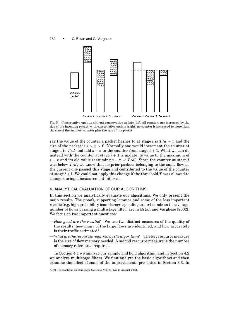
Fig. 5. Conservative update: without conservative update (left) all counters are increased by thesize of the incoming packet, with conservative update (right) no counter is increased to more thanthe size of the smallest counter plus the size of the packet.
say the value of the counter a packet hashes to at stage i is T/d − x and thesize of the packet is s > x > 0. Normally one would increment the counter atstage i to T/d and add s − x to the counter from stage i + 1. What we can doinstead with the counter at stage i + 1 is update its value to the maximum ofs − x and its old value (assuming s − x < T/d ). Since the counter at stage iwas below T/d , we know that no prior packets belonging to the same flow asthe current one passed this stage and contributed to the value of the counterat stage i+ 1. We could not apply this change if the threshold T was allowed tochange during a measurement interval.
4. ANALYTICAL EVALUATION OF OUR ALGORITHMS
In this section we analytically evaluate our algorithms. We only present themain results. The proofs, supporting lemmas and some of the less importantresults (e.g. high probability bounds corresponding to our bounds on the averagenumber of flows passing a multistage filter) are in Estan and Varghese [2002].We focus on two important questions:
—How good are the results? We use two distinct measures of the quality ofthe results: how many of the large flows are identified, and how accuratelyis their traffic estimated?
—What are the resources required by the algorithm? The key resource measureis the size of flow memory needed. A second resource measure is the numberof memory references required.
In Section 4.1 we analyze our sample and hold algorithm, and in Section 4.2we analyze multistage filters. We first analyze the basic algorithms and thenexamine the effect of some of the improvements presented in Section 3.3. In
ACM Transactions on Computer Systems, Vol. 21, No. 3, August 2003.
New Directions in Traffic Measurement and Accounting • 283
the next section (Section 5) we use the results of this section to analyticallycompare our algorithms with sampled NetFlow.
Example. We will use the following running example to give numeric in-stances. Assume a 100 Mbyte/s link with 100, 000 flows. We want to measureall flows whose traffic is more than 1% (1 Mbyte) of link capacity in a one secondmeasurement interval.
4.1 Sample and Hold
We first define some notation used in this section.
— p the probability for sampling a byte;—s the size of a flow (in bytes);—T the threshold for large flows;—C the capacity of the link—the number of bytes that can be sent during the
entire measurement interval;— O the oversampling factor defined by p = O · 1/T ;—c the number of bytes actually counted for a flow.
4.1.1 The Quality of Results for Sample and Hold. The first measure ofthe quality of the results is the probability that a flow at the threshold is notidentified. As presented in Section 3.1 the probability that a flow of size T is notidentified is (1− p)T ≈ e−O . An oversampling factor of 20 results in a probabilityof missing flows at the threshold of 2 ∗ 10−9.
Example. For our example, p must be 1 in 50,000 bytes for an oversamplingof 20. With an average packet size of 500 bytes this is roughly 1 in 100 packets.
The second measure of the quality of the results is the difference betweenthe size of a flow s and our estimate. The number of bytes that go by before thefirst one gets sampled has a geometric probability distribution7: it is x with aprobability8 (1− p)x p.
Therefore E[s − c] = 1/p and SD[s − c] = √1− p/p. The best estimate
for s is c + 1/p and its standard deviation is√
1− p/p. If we choose to use cas an estimate for s then the error will be larger, but we never overestimatethe size of the flow.9 In this case, the deviation from the actual value of s is√
E[(s− c)2] =√2− p/p. Based on this value we can also compute the relativeerror of a flow of size T which is T
√2− p/p =√2− p/O.
Example. For our example, with an oversampling factor O of 20, the relativeerror (computed as the standard deviation of the estimate divided by the actualvalue) for a flow at the threshold is 7%.
7We ignore for simplicity that the bytes before the first sampled byte that are in the same packetwith it are also counted. Therefore the actual algorithm will be more accurate than this model.8Since we focus on large flows, we ignore for simplicity the correction factor that should be appliedto account for the case when the flow goes undetected (i.e. x is actually bound by the size of theflow s, but we ignore this).9Gibbons and Matias [1998] have a more elaborate analysis and use a different correction factor.
ACM Transactions on Computer Systems, Vol. 21, No. 3, August 2003.
284 • C. Estan and G. Varghese
4.1.2 The Memory Requirements for Sample and Hold. The size of the flowmemory is determined by the number of flows identified. The actual number ofsampled packets is an upper bound on the number of entries needed in the flowmemory because new entries are created only for sampled packets. Assumingthat the link is constantly busy, by the linearity of expectation, the expectednumber of sampled bytes is p · C = O · C/T .
Example. Using an oversampling of 20 requires 2,000 entries on average.
The number of sampled bytes can exceed this value. Since the number of sam-pled bytes has a binomial distribution, we can use the normal curve to boundwith high probability the number of bytes sampled during the measurementinterval. Therefore with probability 99% the actual number will be at most2.33 standard deviations above the expected value; similarly, with probability99.9% it will be at most 3.08 standard deviations above the expected value. Thestandard deviation of the number of sampled bytes is
√Cp(1− p).
Example. For an oversampling of 20 and an overflow probability of 0.1% weneed at most 2,147 entries.
This result can be further tightened if we make assumptions about thedistribution of flow sizes and thus account for very large flows having manyof their packets sampled. Let’s assume that the flows have a Zipf (Pareto) dis-tribution with parameter 1 defined as Prs > x = constant ∗ x−1. If we have nflows that use the whole bandwidth C, the total traffic of the largest j flowsis at least C ln( j+1)
ln(2n+1) [Estan and Varghese 2002]. For any value of j between0 and n we obtain an upper bound on the number of entries expected to beused in the flow memory by assuming that the largest j flows always have anentry by having at least one of their packets sampled and each packet sampledfrom the rest of the traffic creates an entry: j +Cp(1− ln( j + 1)/ln(2n+ 1). Bydifferentiating we obtain the value of j that provides the tightest bound: j =Cp/ln(2n+ 1)− 1.
Example. Using an oversampling of 20 requires at most 1,328 entries onaverage.
4.1.3 The Effect of Preserving Entries. We preserve entries across mea-surement intervals to improve accuracy. The probability of missing a large flowdecreases because we cannot miss it if we keep its entry from the prior interval.Accuracy increases because we know the exact size of the flows whose entrieswe keep. To quantify these improvements we need to know the ratio of longlived flows among the large ones.
The cost of this improvement in accuracy is an increase in the size of theflow memory. We need enough memory to hold the samples from both mea-surement intervals.10 Therefore the expected number of entries is bounded by2O · C/T .
10We actually also keep the older entries that are above the threshold. Since we are performinga worst case analysis we assume that there is no flow above the threshold, because if there were,many of its packets would be sampled, decreasing the number of entries required.
ACM Transactions on Computer Systems, Vol. 21, No. 3, August 2003.
New Directions in Traffic Measurement and Accounting • 285
To bound with high probability the number of entries we use the normalcurve and the standard deviation of the number of sampled packets during the2 intervals, which is
√2Cp(1− p).
Example. For an oversampling of 20 and acceptable probability of overflowequal to 0.1%, the flow memory has to have at most 4,207 entries to preserveentries.
4.1.4 The Effect of Early Removal. The effect of early removal on the pro-portion of false negatives depends on whether or not the entries removed earlyare reported. Since we believe it is more realistic that implementations will notreport these entries, we will use this assumption in our analysis. Let R < Tbe the early removal threshold. A flow at the threshold is not reported unlessone of its first T − R bytes is sampled. Therefore the probability of missingthe flow is approximately e−O(T−R)/T . If we use an early removal threshold ofR = 0.2 ∗ T , the probability of missing a large flow is increased from 2 ∗ 10−9
to 1.1 ∗ 10−7 with an oversampling of 20.Early removal reduces the size of the memory required by limiting the num-
ber of entries that are preserved from the previous measurement interval. Sincethere can be at most C/R flows sending R bytes, the number of entries thatwe keep is at most C/R, which can be smaller than OC/T , the bound on theexpected number of sampled packets. The expected number of entries we needis C/R +OC/T .
To bound with high probability the number of entries we use the normalcurve. If R ≥ T/O the standard deviation is given only by the randomness ofthe packets sampled in one interval and is
√Cp(1− p).
Example. An oversampling of 20 and R = 0.2T with overflow probability0.1% requires 2,647 memory entries.
4.2 Multistage Filters
In this section, we analyze parallel multistage filters. We first define some newnotation:
—b the number of buckets in a stage;—d the depth of the filter (the number of stages);—n the number of active flows;—k the stage strength is the ratio of the threshold and the average size of a
counter. k = T bC , where C denotes the channel capacity as before. Intuitively,
this is the factor we inflate by each stage memory beyond the minimum ofC/T .
Example. To illustrate our results numerically, we will assume that wesolve the measurement example described in Section 4 with a 4 stage filter,with 1000 buckets at each stage. The stage strength k is 10 because each stagememory has 10 times more buckets than the maximum number of flows (i.e.,100) that can cross the specified threshold of 1%.
ACM Transactions on Computer Systems, Vol. 21, No. 3, August 2003.
286 • C. Estan and G. Varghese
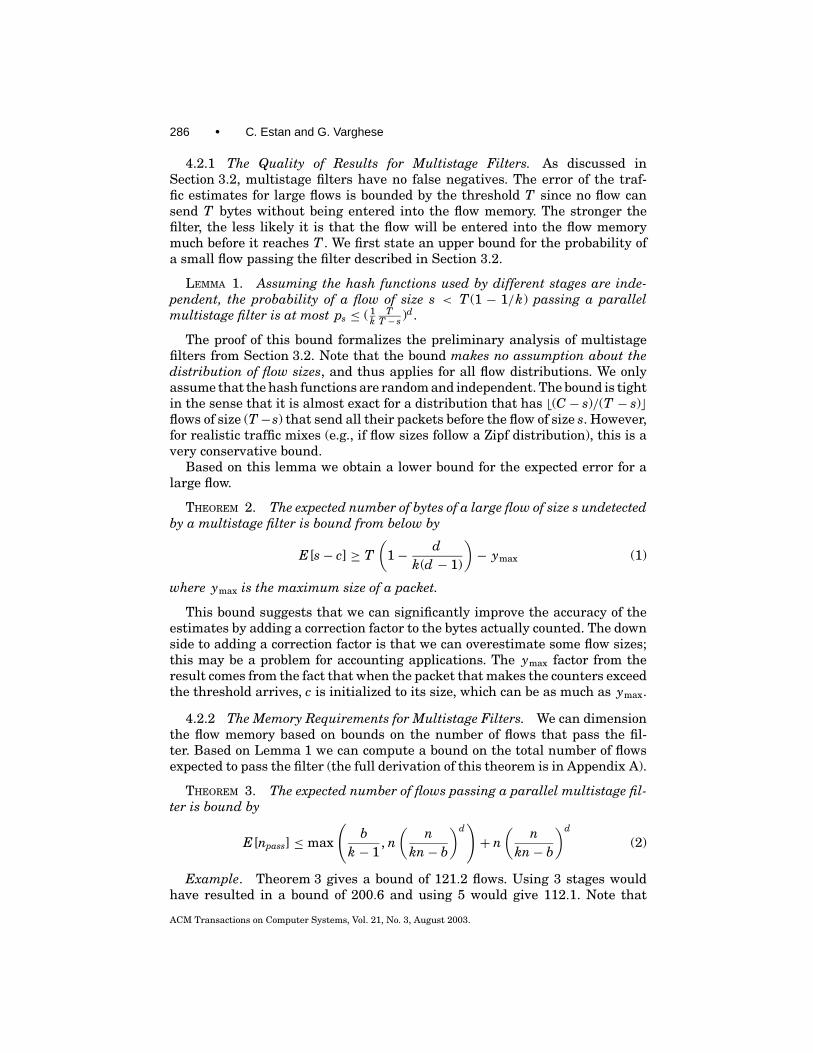
4.2.1 The Quality of Results for Multistage Filters. As discussed inSection 3.2, multistage filters have no false negatives. The error of the traf-fic estimates for large flows is bounded by the threshold T since no flow cansend T bytes without being entered into the flow memory. The stronger thefilter, the less likely it is that the flow will be entered into the flow memorymuch before it reaches T . We first state an upper bound for the probability ofa small flow passing the filter described in Section 3.2.
LEMMA 1. Assuming the hash functions used by different stages are inde-pendent, the probability of a flow of size s < T (1 − 1/k) passing a parallelmultistage filter is at most ps ≤ ( 1
kT
T − s )d .
The proof of this bound formalizes the preliminary analysis of multistagefilters from Section 3.2. Note that the bound makes no assumption about thedistribution of flow sizes, and thus applies for all flow distributions. We onlyassume that the hash functions are random and independent. The bound is tightin the sense that it is almost exact for a distribution that has b(C − s)/(T − s)cflows of size (T−s) that send all their packets before the flow of size s. However,for realistic traffic mixes (e.g., if flow sizes follow a Zipf distribution), this is avery conservative bound.
Based on this lemma we obtain a lower bound for the expected error for alarge flow.
THEOREM 2. The expected number of bytes of a large flow of size s undetectedby a multistage filter is bound from below by
E[s− c] ≥ T(
1− dk(d − 1)
)− ymax (1)
where ymax is the maximum size of a packet.
This bound suggests that we can significantly improve the accuracy of theestimates by adding a correction factor to the bytes actually counted. The downside to adding a correction factor is that we can overestimate some flow sizes;this may be a problem for accounting applications. The ymax factor from theresult comes from the fact that when the packet that makes the counters exceedthe threshold arrives, c is initialized to its size, which can be as much as ymax.
4.2.2 The Memory Requirements for Multistage Filters. We can dimensionthe flow memory based on bounds on the number of flows that pass the fil-ter. Based on Lemma 1 we can compute a bound on the total number of flowsexpected to pass the filter (the full derivation of this theorem is in Appendix A).
THEOREM 3. The expected number of flows passing a parallel multistage fil-ter is bound by
E[npass] ≤ max
(b
k − 1, n(
nkn− b
)d)+ n
(n
kn− b
)d
(2)
Example. Theorem 3 gives a bound of 121.2 flows. Using 3 stages wouldhave resulted in a bound of 200.6 and using 5 would give 112.1. Note that
ACM Transactions on Computer Systems, Vol. 21, No. 3, August 2003.
New Directions in Traffic Measurement and Accounting • 287
when the first term dominates the max, there is not much gain in adding morestages.
We can also bound the number of flows passing the filter with highprobability.
Example. The probability that more than 185 flows pass the filter is at most0.1%. Thus by increasing the flow memory from the expected size of 122 to 185we can make overflow of the flow memory extremely improbable.
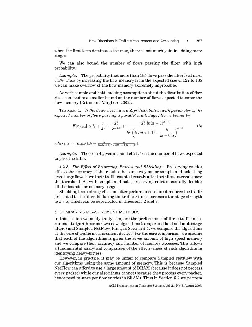
As with sample and hold, making assumptions about the distribution of flowsizes can lead to a smaller bound on the number of flows expected to enter theflow memory [Estan and Varghese 2002].
THEOREM 4. If the flows sizes have a Zipf distribution with parameter 1, theexpected number of flows passing a parallel multistage filter is bound by
E[npass] ≤ i0 + nkd +
dbkd+1 +
db ln(n+ 1)d−2
k2
(k ln(n+ 1)− b
i0 − 0.5
)d−1 (3)
where i0 = dmax(1.5+ bkln(n+ 1) ,
bln(2n+ 1)(k− 1) )e.
Example. Theorem 4 gives a bound of 21.7 on the number of flows expectedto pass the filter.
4.2.3 The Effect of Preserving Entries and Shielding. Preserving entriesaffects the accuracy of the results the same way as for sample and hold: longlived large flows have their traffic counted exactly after their first interval abovethe threshold. As with sample and hold, preserving entries basically doublesall the bounds for memory usage.
Shielding has a strong effect on filter performance, since it reduces the trafficpresented to the filter. Reducing the traffic α times increases the stage strengthto k ∗ α, which can be substituted in Theorems 2 and 3.
5. COMPARING MEASUREMENT METHODS
In this section we analytically compare the performance of three traffic mea-surement algorithms: our two new algorithms (sample and hold and multistagefilters) and Sampled NetFlow. First, in Section 5.1, we compare the algorithmsat the core of traffic measurement devices. For the core comparison, we assumethat each of the algorithms is given the same amount of high speed memoryand we compare their accuracy and number of memory accesses. This allowsa fundamental analytical comparison of the effectiveness of each algorithm inidentifying heavy-hitters.
However, in practice, it may be unfair to compare Sampled NetFlow withour algorithms using the same amount of memory. This is because SampledNetFlow can afford to use a large amount of DRAM (because it does not processevery packet) while our algorithms cannot (because they process every packet,hence need to store per flow entries in SRAM). Thus in Section 5.2 we perform
ACM Transactions on Computer Systems, Vol. 21, No. 3, August 2003.
288 • C. Estan and G. Varghese
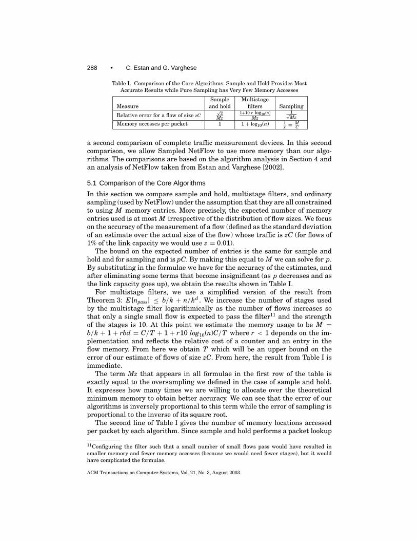
Table I. Comparison of the Core Algorithms: Sample and Hold Provides MostAccurate Results while Pure Sampling has Very Few Memory Accesses
Sample MultistageMeasure and hold filters Sampling
Relative error for a flow of size zC√
2Mz
1+10 r log10(n)Mz
1√Mz
Memory accesses per packet 1 1+ log10(n) 1x = M
C
a second comparison of complete traffic measurement devices. In this secondcomparison, we allow Sampled NetFlow to use more memory than our algo-rithms. The comparisons are based on the algorithm analysis in Section 4 andan analysis of NetFlow taken from Estan and Varghese [2002].
5.1 Comparison of the Core Algorithms
In this section we compare sample and hold, multistage filters, and ordinarysampling (used by NetFlow) under the assumption that they are all constrainedto using M memory entries. More precisely, the expected number of memoryentries used is at most M irrespective of the distribution of flow sizes. We focuson the accuracy of the measurement of a flow (defined as the standard deviationof an estimate over the actual size of the flow) whose traffic is zC (for flows of1% of the link capacity we would use z = 0.01).
The bound on the expected number of entries is the same for sample andhold and for sampling and is pC. By making this equal to M we can solve for p.By substituting in the formulae we have for the accuracy of the estimates, andafter eliminating some terms that become insignificant (as p decreases and asthe link capacity goes up), we obtain the results shown in Table I.
For multistage filters, we use a simplified version of the result fromTheorem 3: E[npass] ≤ b/k + n/kd . We increase the number of stages usedby the multistage filter logarithmically as the number of flows increases sothat only a single small flow is expected to pass the filter11 and the strengthof the stages is 10. At this point we estimate the memory usage to be M =b/k + 1 + rbd = C/T + 1 + r10 log10(n)C/T where r < 1 depends on the im-plementation and reflects the relative cost of a counter and an entry in theflow memory. From here we obtain T which will be an upper bound on theerror of our estimate of flows of size zC. From here, the result from Table I isimmediate.
The term Mz that appears in all formulae in the first row of the table isexactly equal to the oversampling we defined in the case of sample and hold.It expresses how many times we are willing to allocate over the theoreticalminimum memory to obtain better accuracy. We can see that the error of ouralgorithms is inversely proportional to this term while the error of sampling isproportional to the inverse of its square root.
The second line of Table I gives the number of memory locations accessedper packet by each algorithm. Since sample and hold performs a packet lookup
11Configuring the filter such that a small number of small flows pass would have resulted insmaller memory and fewer memory accesses (because we would need fewer stages), but it wouldhave complicated the formulae.
ACM Transactions on Computer Systems, Vol. 21, No. 3, August 2003.
New Directions in Traffic Measurement and Accounting • 289
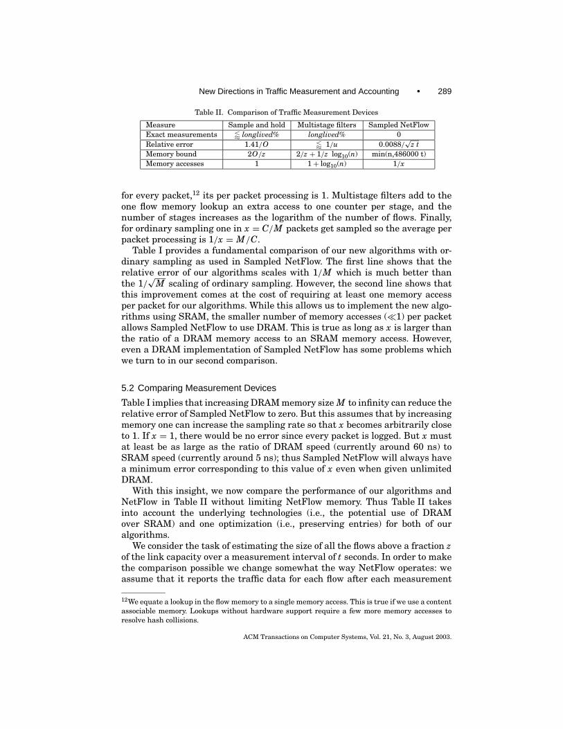
Table II. Comparison of Traffic Measurement Devices
Measure Sample and hold Multistage filters Sampled NetFlowExact measurements / longlived% longlived% 0Relative error 1.41/O / 1/u 0.0088/
√z t
Memory bound 2O/z 2/z + 1/z log10(n) min(n,486000 t)Memory accesses 1 1+ log10(n) 1/x
for every packet,12 its per packet processing is 1. Multistage filters add to theone flow memory lookup an extra access to one counter per stage, and thenumber of stages increases as the logarithm of the number of flows. Finally,for ordinary sampling one in x = C/M packets get sampled so the average perpacket processing is 1/x = M/C.
Table I provides a fundamental comparison of our new algorithms with or-dinary sampling as used in Sampled NetFlow. The first line shows that therelative error of our algorithms scales with 1/M which is much better thanthe 1/
√M scaling of ordinary sampling. However, the second line shows that
this improvement comes at the cost of requiring at least one memory accessper packet for our algorithms. While this allows us to implement the new algo-rithms using SRAM, the smaller number of memory accesses (¿1) per packetallows Sampled NetFlow to use DRAM. This is true as long as x is larger thanthe ratio of a DRAM memory access to an SRAM memory access. However,even a DRAM implementation of Sampled NetFlow has some problems whichwe turn to in our second comparison.
5.2 Comparing Measurement Devices
Table I implies that increasing DRAM memory size M to infinity can reduce therelative error of Sampled NetFlow to zero. But this assumes that by increasingmemory one can increase the sampling rate so that x becomes arbitrarily closeto 1. If x = 1, there would be no error since every packet is logged. But x mustat least be as large as the ratio of DRAM speed (currently around 60 ns) toSRAM speed (currently around 5 ns); thus Sampled NetFlow will always havea minimum error corresponding to this value of x even when given unlimitedDRAM.
With this insight, we now compare the performance of our algorithms andNetFlow in Table II without limiting NetFlow memory. Thus Table II takesinto account the underlying technologies (i.e., the potential use of DRAMover SRAM) and one optimization (i.e., preserving entries) for both of ouralgorithms.
We consider the task of estimating the size of all the flows above a fraction zof the link capacity over a measurement interval of t seconds. In order to makethe comparison possible we change somewhat the way NetFlow operates: weassume that it reports the traffic data for each flow after each measurement
12We equate a lookup in the flow memory to a single memory access. This is true if we use a contentassociable memory. Lookups without hardware support require a few more memory accesses toresolve hash collisions.
ACM Transactions on Computer Systems, Vol. 21, No. 3, August 2003.
290 • C. Estan and G. Varghese
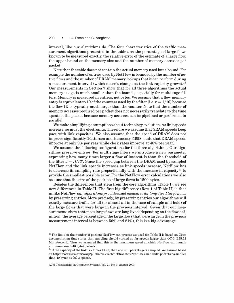
interval, like our algorithms do. The four characteristics of the traffic mea-surement algorithms presented in the table are: the percentage of large flowsknown to be measured exactly, the relative error of the estimate of a large flow,the upper bound on the memory size and the number of memory accesses perpacket.
Note that the table does not contain the actual memory used but a bound. Forexample the number of entries used by NetFlow is bounded by the number of ac-tive flows and the number of DRAM memory lookups that it can perform duringa measurement interval (which doesn’t change as the link capacity grows).13
Our measurements in Section 7 show that for all three algorithms the actualmemory usage is much smaller than the bounds, especially for multistage fil-ters. Memory is measured in entries, not bytes. We assume that a flow memoryentry is equivalent to 10 of the counters used by the filter (i.e. r = 1/10) becausethe flow ID is typically much larger than the counter. Note that the number ofmemory accesses required per packet does not necessarily translate to the timespent on the packet because memory accesses can be pipelined or performed inparallel.
We make simplifying assumptions about technology evolution. As link speedsincrease, so must the electronics. Therefore we assume that SRAM speeds keeppace with link capacities. We also assume that the speed of DRAM does notimprove significantly (Patterson and Hennessy [1998] state that DRAM speedsimprove at only 9% per year while clock rates improve at 40% per year).
We assume the following configurations for the three algorithms. Our algo-rithms preserve entries. For multistage filters we introduce a new parameterexpressing how many times larger a flow of interest is than the threshold ofthe filter u = zC/T . Since the speed gap between the DRAM used by sampledNetFlow and the link speeds increases as link speeds increase, NetFlow hasto decrease its sampling rate proportionally with the increase in capacity14 toprovide the smallest possible error. For the NetFlow error calculations we alsoassume that the size of the packets of large flows is 1500 bytes.
Besides the differences that stem from the core algorithms (Table I), we seenew differences in Table II. The first big difference (Row 1 of Table II) is thatunlike NetFlow, our algorithms provide exact measures for long-lived large flowsby preserving entries. More precisely, by preserving entries our algorithms willexactly measure traffic for all (or almost all in the case of sample and hold) ofthe large flows that were large in the previous interval. Given that our mea-surements show that most large flows are long lived (depending on the flow def-inition, the average percentage of the large flows that were large in the previousmeasurement interval is between 56% and 81%), this is a big advantage.
13The limit on the number of packets NetFlow can process we used for Table II is based on Ciscodocumentation that states that sampling should turned on for speeds larger than OC-3 (155.52Mbits/second). Thus we assumed that this is the maximum speed at which NetFlow can handleminimum sized (40 byte) packets.14If the capacity of the link is x times OC-3, then one in x packets gets sampled. We assume basedon http://www.cisco.com/warp/public/732/Tech/netflow that NetFlow can handle packets no smallerthan 40 bytes at OC-3 speeds.
ACM Transactions on Computer Systems, Vol. 21, No. 3, August 2003.
New Directions in Traffic Measurement and Accounting • 291
Of course, one could get the same advantage by using an SRAM flow memorythat preserves large flows across measurement intervals in Sampled NetFlow.However, that would require the router to root through its DRAM flow memorybefore the end of the interval to find the large flows, a large processing load.One can also argue that if one can afford an SRAM flow memory, it is quite easyto do sample and hold.
The second big difference (Row 2 of Table II) is that we can make our algo-rithms arbitrarily accurate at the cost of increases in the amount of memoryused15 while sampled NetFlow can do so only by increasing the measurementinterval t.
The third row of Table II compares the memory used by the algorithms.The extra factor of 2 for sample and hold and multistage filters arises frompreserving entries. Note that the number of entries used by Sampled NetFlowis bounded by both the number n of active flows and the number of memoryaccesses that can be made in t seconds. Finally, the fourth row of Table II isidentical to the second row of Table I.
Table II demonstrates that our algorithms have two advantages over Net-Flow: i) they provide exact values for long-lived large flows (row 1) and ii) theyprovide much better accuracy even for small measurement intervals (row 2). Be-sides these, our algorithms have three more advantages not shown in Table II.These are iii) provable lower bounds on traffic, iv) reduced resource consump-tion for collection, and v) faster detection of new large flows. We now examineadvantages iii) through v) in more detail.
iii) Provable Lower Bounds: A possible disadvantage of Sampled Net-Flow is that the NetFlow estimate is not an actual lower bound on the flowsize. Thus a customer may be charged for more than the customer sends. Whileone can make the probability of overcharging arbitrarily low (using large mea-surement intervals or other methods from Duffield et al. [2001]), there maybe philosophical objections to overcharging. Our algorithms do not have thisproblem.
iv) Reduced Resource Consumption: Clearly, while Sampled NetFlowcan increase DRAM to improve accuracy, the router has more entries at the endof the measurement interval. These records have to be processed, potentiallyaggregated, and transmitted over the network to the management station. If therouter extracts the heavy hitters from the log, then router processing is large;if not, the bandwidth consumed and processing at the management station arelarge. By using fewer entries, our algorithms avoid these resource (e.g., memory,transmission bandwidth, and router CPU cycles) bottlenecks, but as detailedin Table II sample and hold and multistage filters incur more upfront work byprocessing each packet.
6. DIMENSIONING TRAFFIC MEASUREMENT DEVICES
We describe how to dimension our algorithms. For applications that face adver-sarial behavior (e.g., detecting DoS attacks), one should use the conservative
15Of course, technology and cost impose limitations on the amount of available SRAM but thecurrent limits for on and off-chip SRAM are high enough for our algorithms.
ACM Transactions on Computer Systems, Vol. 21, No. 3, August 2003.
292 • C. Estan and G. Varghese
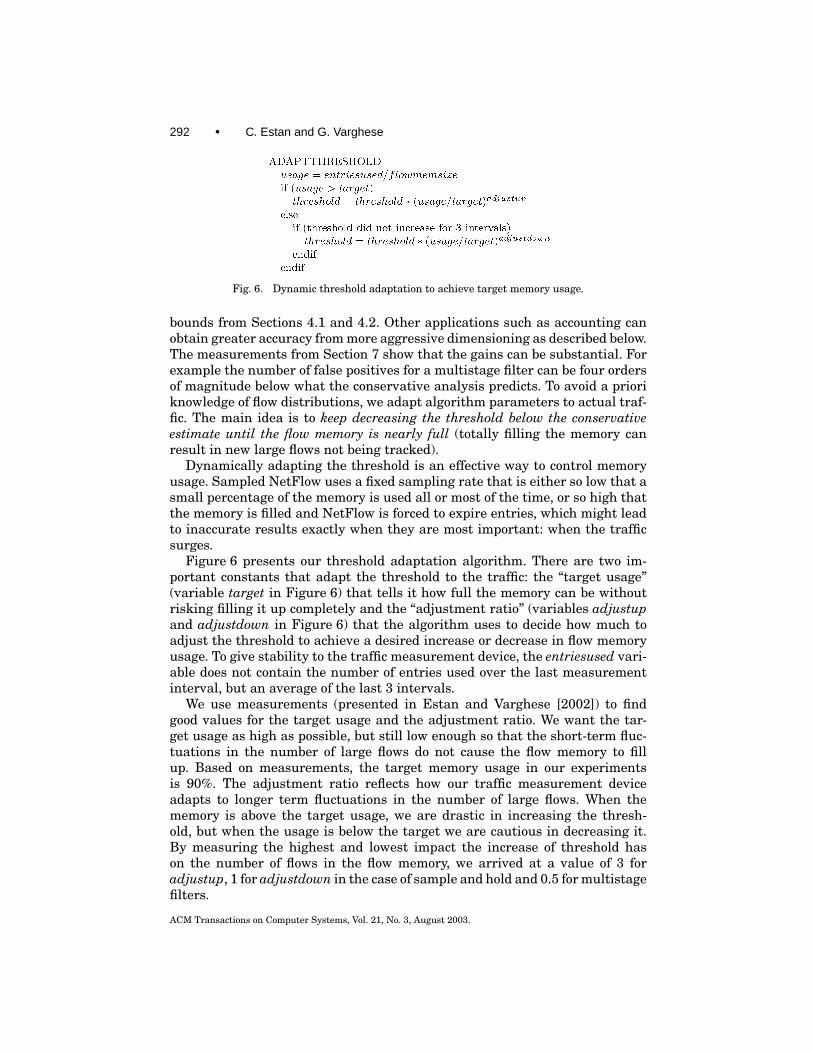
Fig. 6. Dynamic threshold adaptation to achieve target memory usage.
bounds from Sections 4.1 and 4.2. Other applications such as accounting canobtain greater accuracy from more aggressive dimensioning as described below.The measurements from Section 7 show that the gains can be substantial. Forexample the number of false positives for a multistage filter can be four ordersof magnitude below what the conservative analysis predicts. To avoid a prioriknowledge of flow distributions, we adapt algorithm parameters to actual traf-fic. The main idea is to keep decreasing the threshold below the conservativeestimate until the flow memory is nearly full (totally filling the memory canresult in new large flows not being tracked).
Dynamically adapting the threshold is an effective way to control memoryusage. Sampled NetFlow uses a fixed sampling rate that is either so low that asmall percentage of the memory is used all or most of the time, or so high thatthe memory is filled and NetFlow is forced to expire entries, which might leadto inaccurate results exactly when they are most important: when the trafficsurges.
Figure 6 presents our threshold adaptation algorithm. There are two im-portant constants that adapt the threshold to the traffic: the “target usage”(variable target in Figure 6) that tells it how full the memory can be withoutrisking filling it up completely and the “adjustment ratio” (variables adjustupand adjustdown in Figure 6) that the algorithm uses to decide how much toadjust the threshold to achieve a desired increase or decrease in flow memoryusage. To give stability to the traffic measurement device, the entriesused vari-able does not contain the number of entries used over the last measurementinterval, but an average of the last 3 intervals.
We use measurements (presented in Estan and Varghese [2002]) to findgood values for the target usage and the adjustment ratio. We want the tar-get usage as high as possible, but still low enough so that the short-term fluc-tuations in the number of large flows do not cause the flow memory to fillup. Based on measurements, the target memory usage in our experimentsis 90%. The adjustment ratio reflects how our traffic measurement deviceadapts to longer term fluctuations in the number of large flows. When thememory is above the target usage, we are drastic in increasing the thresh-old, but when the usage is below the target we are cautious in decreasing it.By measuring the highest and lowest impact the increase of threshold hason the number of flows in the flow memory, we arrived at a value of 3 foradjustup, 1 for adjustdown in the case of sample and hold and 0.5 for multistagefilters.
ACM Transactions on Computer Systems, Vol. 21, No. 3, August 2003.
New Directions in Traffic Measurement and Accounting • 293
6.1 Dimensioning the Multistage Filter
Even if we have the correct constants for the threshold adaptation algorithm,there are other configuration parameters for the multistage filter we need toset. Our aim in this section is not to derive the exact optimal values for theconfiguration parameters of the multistage filters. Due to the dynamic thresholdadaptation, the device will work even if we use suboptimal values. Neverthelesswe want to avoid using configuration parameters that would lead the dynamicadaptation to stabilize at a value of the threshold that is significantly higherthan the one for the optimal configuration.
We assume that design constraints limit the total amount of memory we canuse for the stage counters and the flow memory, but we have no restrictionson how to divide it between the filter and the flow memory. Since the numberof per packet memory accesses might be limited, we assume that we mighthave a limit on the number of stages. We want to see how we should dividethe available memory between the filter and the flow memory and how manystages to use. We base our configuration parameters on some knowledge of thetraffic mix (the number of active flows and the percentage of large flows thatare long lived).
We first introduce a simplified model of how the multistage filter works. Mea-surements confirm this model is closer to the actual behavior of the filters thanthe conservative analysis. Because of shielding the old large flows do not affectthe filter. We assume that because of conservative update only the countersto which the new large flows hash reach the threshold. Let l be the numberof large flows and 1l be the number of new large flows. We approximate theprobability of a small flow passing one stage by 1l/b and of passing the wholefilter by (1l/b)d . This gives us the number of false positives in each intervalfp = n(1l/b)d . The number of memory locations used at the end of a measure-ment interval consists of the large flows and the false positives of the previousinterval and the new large flows and the new false positives m = l +1l +2∗ fp.To be able to establish a tradeoff between using the available memory for thefilter or the flow memory, we need to know the relative cost of a counter anda flow entry. Let r denote the ratio between the size of a counter and the sizeof an entry. The amount of memory used by the filter is going to be equivalentto b ∗ d ∗ r entries. To determine the optimal number of counters per stagegiven a certain number of large flows, new large flows, and stages, we take thederivative of the total memory with respect to b. Equation 4 gives the optimalvalue for b and Equation 5 gives the total amount of memory required with thischoice of b.
b = 1l d+1
√2n
r1l(4)
mtotal = l +1l + (d + 1) r1l d+1
√2n
r1l(5)
We make a further simplifying assumption that the ratio between 1l and l(related to the flow arrival rate) doesn’t depend on the threshold. Measurements
ACM Transactions on Computer Systems, Vol. 21, No. 3, August 2003.
294 • C. Estan and G. Varghese
confirm that this is a good approximation for wide ranges of the threshold. Forthe MAG trace, when we define the flows at the granularity of TCP connections1l/l is around 44%, when defining flows based on destination IP 37% and whendefining them as AS pairs 19%. Let M be the number of entries the availablememory can hold. We solve Equation 5 with respect to l for all possible valuesof d from 2 to the limit on the number of memory accesses we can afford perpacket. We choose the depth of the filter that gives the largest l and compute bbased on that value.
7. MEASUREMENTS
In Section 4 and Section 5 we used theoretical analysis to understand the ef-fectiveness of our algorithms. In this section, we turn to experimental analysisto show that our algorithms behave much better on real traces than the (rea-sonably good) bounds provided by the earlier theoretical analysis and comparethem with Sampled NetFlow.
We start by describing the traces we use and some of the configuration de-tails common to all our experiments. In Section 7.1.1 we compare the measuredperformance of the sample and hold algorithm with the predictions of the an-alytical evaluation, and also evaluate how much the various improvementsto the basic algorithm help. In Section 7.1.2 we evaluate the multistage filterand the improvements that apply to it. We conclude with Section 7.2 where wecompare complete traffic measurement devices using our two algorithms withCisco’s Sampled NetFlow.
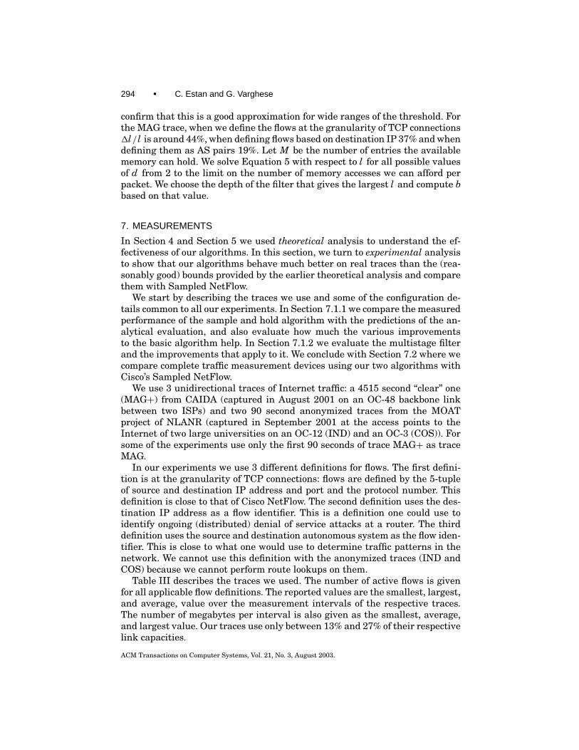
We use 3 unidirectional traces of Internet traffic: a 4515 second “clear” one(MAG+) from CAIDA (captured in August 2001 on an OC-48 backbone linkbetween two ISPs) and two 90 second anonymized traces from the MOATproject of NLANR (captured in September 2001 at the access points to theInternet of two large universities on an OC-12 (IND) and an OC-3 (COS)). Forsome of the experiments use only the first 90 seconds of trace MAG+ as traceMAG.
In our experiments we use 3 different definitions for flows. The first defini-tion is at the granularity of TCP connections: flows are defined by the 5-tupleof source and destination IP address and port and the protocol number. Thisdefinition is close to that of Cisco NetFlow. The second definition uses the des-tination IP address as a flow identifier. This is a definition one could use toidentify ongoing (distributed) denial of service attacks at a router. The thirddefinition uses the source and destination autonomous system as the flow iden-tifier. This is close to what one would use to determine traffic patterns in thenetwork. We cannot use this definition with the anonymized traces (IND andCOS) because we cannot perform route lookups on them.
Table III describes the traces we used. The number of active flows is givenfor all applicable flow definitions. The reported values are the smallest, largest,and average, value over the measurement intervals of the respective traces.The number of megabytes per interval is also given as the smallest, average,and largest value. Our traces use only between 13% and 27% of their respectivelink capacities.
ACM Transactions on Computer Systems, Vol. 21, No. 3, August 2003.
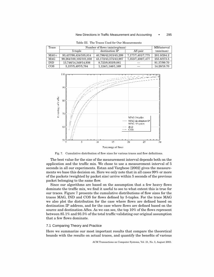
New Directions in Traffic Measurement and Accounting • 295
Table III. The Traces Used for Our Measurements
Trace Number of flows (min/avg/max) MB/interval5-tuple destination IP AS pair (min/max)
MAG+ 93,437/98,424/105,814 40,796/42,915/45,299 7,177/7,401/7,775 201.0/284.2MAG 99,264/100,105/101,038 43,172/43,575/43,987 7,353/7,408/7,477 255.8/273.5IND 13,746/14,349/14,936 8,723/8,933/9,081 — 91.37/99.70COS 5,157/5,497/5,784 1,124/1,146/1,169 — 14.28/18.70
Fig. 7. Cumulative distribution of flow sizes for various traces and flow definitions.
The best value for the size of the measurement interval depends both on theapplication and the traffic mix. We chose to use a measurement interval of 5seconds in all our experiments. Estan and Varghese [2002] gives the measure-ments we base this decision on. Here we only note that in all cases 99% or moreof the packets (weighted by packet size) arrive within 5 seconds of the previouspacket belonging to the same flow.
Since our algorithms are based on the assumption that a few heavy flowsdominate the traffic mix, we find it useful to see to what extent this is true forour traces. Figure 7 presents the cumulative distributions of flow sizes for thetraces MAG, IND and COS for flows defined by 5-tuples. For the trace MAGwe also plot the distribution for the case where flows are defined based ondestination IP address, and for the case where flows are defined based on thesource and destination ASes. As we can see, the top 10% of the flows representbetween 85.1% and 93.5% of the total traffic validating our original assumptionthat a few flows dominate.
7.1 Comparing Theory and Practice
Here we summarize our most important results that compare the theoreticalbounds with the results on actual traces, and quantify the benefits of various
ACM Transactions on Computer Systems, Vol. 21, No. 3, August 2003.
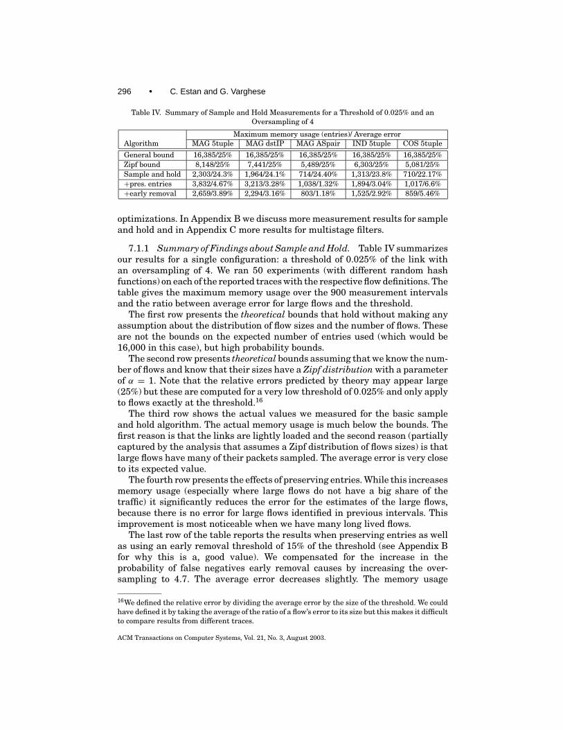
296 • C. Estan and G. Varghese
Table IV. Summary of Sample and Hold Measurements for a Threshold of 0.025% and anOversampling of 4
Maximum memory usage (entries)/ Average errorAlgorithm MAG 5tuple MAG dstIP MAG ASpair IND 5tuple COS 5tuple
General bound 16,385/25% 16,385/25% 16,385/25% 16,385/25% 16,385/25%Zipf bound 8,148/25% 7,441/25% 5,489/25% 6,303/25% 5,081/25%Sample and hold 2,303/24.3% 1,964/24.1% 714/24.40% 1,313/23.8% 710/22.17%+pres. entries 3,832/4.67% 3,213/3.28% 1,038/1.32% 1,894/3.04% 1,017/6.6%+early removal 2,659/3.89% 2,294/3.16% 803/1.18% 1,525/2.92% 859/5.46%
optimizations. In Appendix B we discuss more measurement results for sampleand hold and in Appendix C more results for multistage filters.
7.1.1 Summary of Findings about Sample and Hold. Table IV summarizesour results for a single configuration: a threshold of 0.025% of the link withan oversampling of 4. We ran 50 experiments (with different random hashfunctions) on each of the reported traces with the respective flow definitions. Thetable gives the maximum memory usage over the 900 measurement intervalsand the ratio between average error for large flows and the threshold.
The first row presents the theoretical bounds that hold without making anyassumption about the distribution of flow sizes and the number of flows. Theseare not the bounds on the expected number of entries used (which would be16,000 in this case), but high probability bounds.
The second row presents theoretical bounds assuming that we know the num-ber of flows and know that their sizes have a Zipf distribution with a parameterof α = 1. Note that the relative errors predicted by theory may appear large(25%) but these are computed for a very low threshold of 0.025% and only applyto flows exactly at the threshold.16
The third row shows the actual values we measured for the basic sampleand hold algorithm. The actual memory usage is much below the bounds. Thefirst reason is that the links are lightly loaded and the second reason (partiallycaptured by the analysis that assumes a Zipf distribution of flows sizes) is thatlarge flows have many of their packets sampled. The average error is very closeto its expected value.
The fourth row presents the effects of preserving entries. While this increasesmemory usage (especially where large flows do not have a big share of thetraffic) it significantly reduces the error for the estimates of the large flows,because there is no error for large flows identified in previous intervals. Thisimprovement is most noticeable when we have many long lived flows.
The last row of the table reports the results when preserving entries as wellas using an early removal threshold of 15% of the threshold (see Appendix Bfor why this is a, good value). We compensated for the increase in theprobability of false negatives early removal causes by increasing the over-sampling to 4.7. The average error decreases slightly. The memory usage
16We defined the relative error by dividing the average error by the size of the threshold. We couldhave defined it by taking the average of the ratio of a flow’s error to its size but this makes it difficultto compare results from different traces.
ACM Transactions on Computer Systems, Vol. 21, No. 3, August 2003.
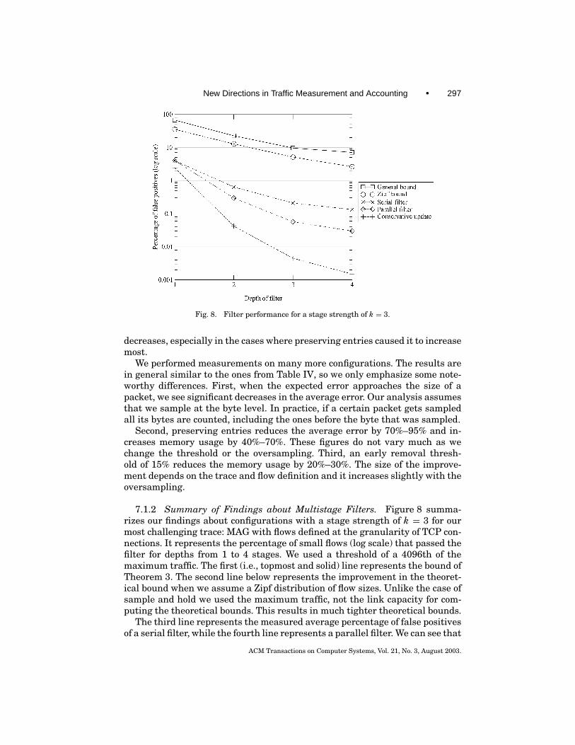
New Directions in Traffic Measurement and Accounting • 297
Fig. 8. Filter performance for a stage strength of k = 3.
decreases, especially in the cases where preserving entries caused it to increasemost.
We performed measurements on many more configurations. The results arein general similar to the ones from Table IV, so we only emphasize some note-worthy differences. First, when the expected error approaches the size of apacket, we see significant decreases in the average error. Our analysis assumesthat we sample at the byte level. In practice, if a certain packet gets sampledall its bytes are counted, including the ones before the byte that was sampled.
Second, preserving entries reduces the average error by 70%–95% and in-creases memory usage by 40%–70%. These figures do not vary much as wechange the threshold or the oversampling. Third, an early removal thresh-old of 15% reduces the memory usage by 20%–30%. The size of the improve-ment depends on the trace and flow definition and it increases slightly with theoversampling.
7.1.2 Summary of Findings about Multistage Filters. Figure 8 summa-rizes our findings about configurations with a stage strength of k = 3 for ourmost challenging trace: MAG with flows defined at the granularity of TCP con-nections. It represents the percentage of small flows (log scale) that passed thefilter for depths from 1 to 4 stages. We used a threshold of a 4096th of themaximum traffic. The first (i.e., topmost and solid) line represents the bound ofTheorem 3. The second line below represents the improvement in the theoret-ical bound when we assume a Zipf distribution of flow sizes. Unlike the case ofsample and hold we used the maximum traffic, not the link capacity for com-puting the theoretical bounds. This results in much tighter theoretical bounds.
The third line represents the measured average percentage of false positivesof a serial filter, while the fourth line represents a parallel filter. We can see that
ACM Transactions on Computer Systems, Vol. 21, No. 3, August 2003.

298 • C. Estan and G. Varghese
both are at least 10 times better than the stronger of the theoretical bounds.As the number of stages goes up, the parallel filter gets better than the serialfilter by up to a factor of 4. The last line represents a parallel filter with con-servative update, which gets progressively better than the parallel filter by upto a factor of 20 as the number of stages increases. We can see that all lines areroughly straight; this indicates that the percentage of false positives decreasesexponentially with the number of stages.
Measurements on other traces show similar results. The difference betweenthe bounds and measured performance is even larger for the traces where thelargest flows are responsible for a large share of the traffic. With conservativeupdate and without preserving entries the average error is very close to thethreshold. Preserving entries reduces the average error in the estimates by70% to 85% because the estimates for long lived flows are exact in all but thefirst measurement interval. The improvements in the results due to preservingentries depend on the traffic mix. Preserving entries increases the number offlow memory entries used by up to 30%. By effectively increasing stage strengthk, shielding considerably strengthens weak filters. This can lead to reducingthe number of entries by as much as 70%.
7.2 Evaluation of Complete Traffic Measurement Devices
We now present our final comparison between sample and hold, multistagefilters, and sampled NetFlow. We perform the evaluation on our long OC-48trace, MAG+. We assume that our devices can use 1 Mbit of memory (4096entries17), which is well within the possibilities of today’s chips. Sampled Net-Flow is given unlimited memory and uses a sampling of 1 in 16 packets. Werun each algorithm 16 times on the trace with different sampling or hashfunctions.
Both our algorithms use the adaptive threshold approach. To avoid the effectof initial misconfiguration, we ignore the first 10 intervals to give the devicestime to reach a relatively stable value for the threshold. We impose a limit of 4stages for the multistage filters. Based on heuristics presented in Section 6.1,we use 3114 counters18 for each stage and 2539 entries of flow memory whenusing a flow definition at the granularity of TCP connections, 2646 counters and2773 entries when using the destination IP as flow identifier and 1502 countersand 3345 entries when using the source and destination AS. Multistage filtersuse shielding and conservative update. Sample and hold uses an oversamplingof 4 and an early removal threshold of 15%.
Our purpose is to see how accurately the algorithms measure the largestflows, but there is no implicit definition of what large flows are. We look sep-arately at how well the devices perform for three reference groups: very largeflows (above one thousandth of the link capacity), large flows (between onethousandth and a tenth of a thousandth) and medium flows (between a tenthof a thousandth and a hundredth of a thousandth—15,552 bytes).
17Cisco NetFlow uses 64 bytes per entry in cheap DRAM. We conservatively assume that the sizeof a flow memory entry will be 32 bytes (even though 16 or 24 are also plausible).18We conservatively assume that we use 4 bytes for a counter even though 3 bytes would be enough.
ACM Transactions on Computer Systems, Vol. 21, No. 3, August 2003.
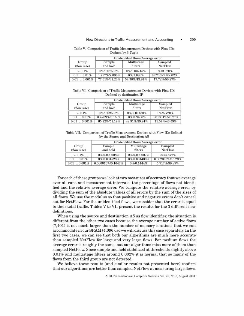
New Directions in Traffic Measurement and Accounting • 299
Table V. Comparison of Traffic Measurement Devices with Flow IDsDefined by 5-Tuple
Unidentified flows/Average errorGroup Sample Multistage Sampled
(flow size) and hold filters NetFlow
> 0.1% 0%/0.07508% 0%/0.03745% 0%/9.020%0.1 . . .0.01% 1.797%/7.086% 0%/1.090% 0.02132%/22.02%
0.01 . . .0.001% 77.01%/61.20% 54.70%/43.87% 17.72%/50.27%
Table VI. Comparison of Traffic Measurement Devices with Flow IDsDefined by destination IP
Unidentified flows/Average errorGroup Sample Multistage Sampled
(flow size) and hold filters NetFlow
> 0.1% 0%/0.02508% 0%/0.01430% 0%/5.720%0.1 . . .0.01% 0.4289%/3.153% 0%/0.9488% 0.01381%/20.77%
0.01 . . .0.001% 65.72%/51.19% 49.91%/39.91% 11.54%/46.59%
Table VII. Comparison of Traffic Measurement Devices with Flow IDs Definedby the Source and Destination AS
Unidentified flows/Average errorGroup Sample Multistage Sampled
(flow size) and hold filters NetFlow
> 0.1% 0%/0.000008% 0%/0.000007% 0%/4.877%0.1 . . .0.01% 0%/0.001528% 0%/0.001403% 0.002005%/15.28%
0.01 . . .0.001% 0.000016%/0.1647% 0%/0.1444% 5.717%/39.87%
For each of these groups we look at two measures of accuracy that we averageover all runs and measurement intervals: the percentage of flows not identi-fied and the relative average error. We compute the relative average error bydividing the sum of the absolute values of all errors by the sum of the sizes ofall flows. We use the modulus so that positive and negative errors don’t cancelout for NetFlow. For the unidentified flows, we consider that the error is equalto their total traffic. Tables V to VII present the results for the 3 different flowdefinitions.
When using the source and destination AS as flow identifier, the situation isdifferent from the other two cases because the average number of active flows(7,401) is not much larger than the number of memory locations that we canaccommodate in our SRAM (4,096), so we will discuss this case separately. In thefirst two cases, we can see that both our algorithms are much more accuratethan sampled NetFlow for large and very large flows. For medium flows theaverage error is roughly the same, but our algorithms miss more of them thansampled NetFlow. Since sample and hold stabilized at thresholds slightly above0.01% and multistage filters around 0.002% it is normal that so many of theflows from the third group are not detected.
We believe these results (and similar results not presented here) confirmthat our algorithms are better than sampled NetFlow at measuring large flows.
ACM Transactions on Computer Systems, Vol. 21, No. 3, August 2003.
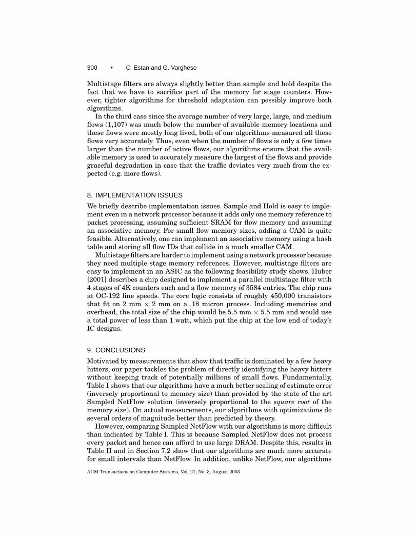
300 • C. Estan and G. Varghese
Multistage filters are always slightly better than sample and hold despite thefact that we have to sacrifice part of the memory for stage counters. How-ever, tighter algorithms for threshold adaptation can possibly improve bothalgorithms.
In the third case since the average number of very large, large, and mediumflows (1,107) was much below the number of available memory locations andthese flows were mostly long lived, both of our algorithms measured all theseflows very accurately. Thus, even when the number of flows is only a few timeslarger than the number of active flows, our algorithms ensure that the avail-able memory is used to accurately measure the largest of the flows and providegraceful degradation in case that the traffic deviates very much from the ex-pected (e.g. more flows).
8. IMPLEMENTATION ISSUES
We briefly describe implementation issues. Sample and Hold is easy to imple-ment even in a network processor because it adds only one memory reference topacket processing, assuming sufficient SRAM for flow memory and assumingan associative memory. For small flow memory sizes, adding a CAM is quitefeasible. Alternatively, one can implement an associative memory using a hashtable and storing all flow IDs that collide in a much smaller CAM.
Multistage filters are harder to implement using a network processor becausethey need multiple stage memory references. However, multistage filters areeasy to implement in an ASIC as the following feasibility study shows. Huber[2001] describes a chip designed to implement a parallel multistage filter with4 stages of 4K counters each and a flow memory of 3584 entries. The chip runsat OC-192 line speeds. The core logic consists of roughly 450,000 transistorsthat fit on 2 mm × 2 mm on a .18 micron process. Including memories andoverhead, the total size of the chip would be 5.5 mm × 5.5 mm and would usea total power of less than 1 watt, which put the chip at the low end of today’sIC designs.
9. CONCLUSIONS
Motivated by measurements that show that traffic is dominated by a few heavyhitters, our paper tackles the problem of directly identifying the heavy hitterswithout keeping track of potentially millions of small flows. Fundamentally,Table I shows that our algorithms have a much better scaling of estimate error(inversely proportional to memory size) than provided by the state of the artSampled NetFlow solution (inversely proportional to the square root of thememory size). On actual measurements, our algorithms with optimizations doseveral orders of magnitude better than predicted by theory.
However, comparing Sampled NetFlow with our algorithms is more difficultthan indicated by Table I. This is because Sampled NetFlow does not processevery packet and hence can afford to use large DRAM. Despite this, results inTable II and in Section 7.2 show that our algorithms are much more accuratefor small intervals than NetFlow. In addition, unlike NetFlow, our algorithms
ACM Transactions on Computer Systems, Vol. 21, No. 3, August 2003.
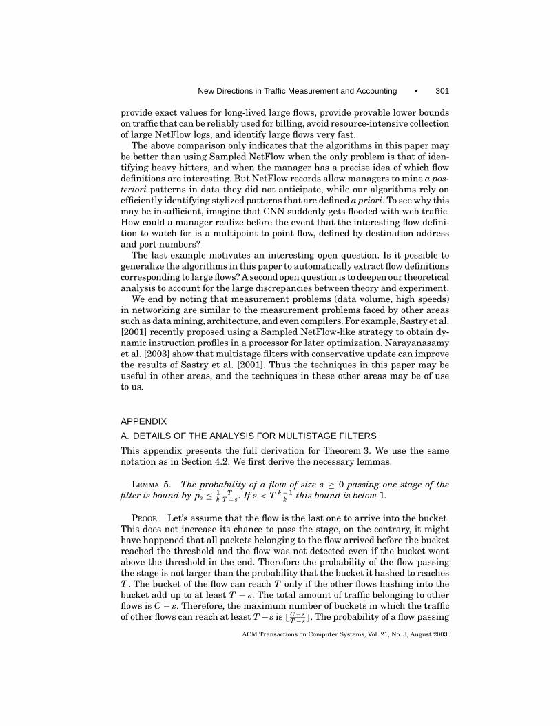
New Directions in Traffic Measurement and Accounting • 301
provide exact values for long-lived large flows, provide provable lower boundson traffic that can be reliably used for billing, avoid resource-intensive collectionof large NetFlow logs, and identify large flows very fast.
The above comparison only indicates that the algorithms in this paper maybe better than using Sampled NetFlow when the only problem is that of iden-tifying heavy hitters, and when the manager has a precise idea of which flowdefinitions are interesting. But NetFlow records allow managers to mine a pos-teriori patterns in data they did not anticipate, while our algorithms rely onefficiently identifying stylized patterns that are defined a priori. To see why thismay be insufficient, imagine that CNN suddenly gets flooded with web traffic.How could a manager realize before the event that the interesting flow defini-tion to watch for is a multipoint-to-point flow, defined by destination addressand port numbers?
The last example motivates an interesting open question. Is it possible togeneralize the algorithms in this paper to automatically extract flow definitionscorresponding to large flows? A second open question is to deepen our theoreticalanalysis to account for the large discrepancies between theory and experiment.
We end by noting that measurement problems (data volume, high speeds)in networking are similar to the measurement problems faced by other areassuch as data mining, architecture, and even compilers. For example, Sastry et al.[2001] recently proposed using a Sampled NetFlow-like strategy to obtain dy-namic instruction profiles in a processor for later optimization. Narayanasamyet al. [2003] show that multistage filters with conservative update can improvethe results of Sastry et al. [2001]. Thus the techniques in this paper may beuseful in other areas, and the techniques in these other areas may be of useto us.
APPENDIX
A. DETAILS OF THE ANALYSIS FOR MULTISTAGE FILTERS
This appendix presents the full derivation for Theorem 3. We use the samenotation as in Section 4.2. We first derive the necessary lemmas.
LEMMA 5. The probability of a flow of size s ≥ 0 passing one stage of thefilter is bound by ps ≤ 1
kT
T − s . If s < T k− 1k this bound is below 1.
PROOF. Let’s assume that the flow is the last one to arrive into the bucket.This does not increase its chance to pass the stage, on the contrary, it mighthave happened that all packets belonging to the flow arrived before the bucketreached the threshold and the flow was not detected even if the bucket wentabove the threshold in the end. Therefore the probability of the flow passingthe stage is not larger than the probability that the bucket it hashed to reachesT . The bucket of the flow can reach T only if the other flows hashing into thebucket add up to at least T − s. The total amount of traffic belonging to otherflows is C − s. Therefore, the maximum number of buckets in which the trafficof other flows can reach at least T−s is bC− s
T − sc. The probability of a flow passing
ACM Transactions on Computer Systems, Vol. 21, No. 3, August 2003.
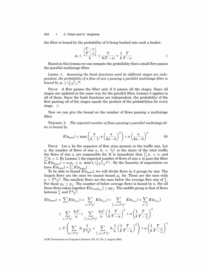
302 • C. Estan and G. Varghese
the filter is bound by the probability of it being hashed into such a bucket.
ps ≤
⌊C − sT − s
⌋b
≤ Cb(T − s)
= 1k
TT − s
Based on this lemma we can compute the probability that a small flow passesthe parallel multistage filter.
LEMMA 1. Assuming the hash functions used by different stages are inde-pendent, the probability of a flow of size s passing a parallel multistage filter isbound by ps ≤ ( 1
kT
T − s )d .
PROOF. A flow passes the filter only if it passes all the stages. Since allstages are updated in the same way for the parallel filter, Lemma 5 applies toall of them. Since the hash functions are independent, the probability of theflow passing all of the stages equals the product of the probabilities for everystage.
Now we can give the bound on the number of flows passing a multistagefilter.
THEOREM 3. The expected number of flows passing a parallel multistage fil-ter is bound by
E[npass] ≤ max
(b
k − 1, n(
nkn− b
)d)+ n
(n
kn− b
)d
(6)
PROOF. Let si be the sequence of flow sizes present in the traffic mix. Letni the number of flows of size si. hi = ni si
C is the share of the total trafficthe flows of size si are responsible for. It is immediate that
∑ni = n, and∑
hi = 1. By Lemma 1 the expected number of flows of size si to pass the filteris E[nipass] = ni psi ≤ ni min(1, ( 1
kT
T − si)d ) . By the linearity of expectation we
have E[npass] =∑
E[nipass ] .To be able to bound E[npass], we will divide flows in 3 groups by size. The
largest flows are the ones we cannot bound psi for. These are the ones withsi > T k− 1
k . The smallest flows are the ones below the average flow size of Cn .
For these psi ≤ pCn. The number of below average flows is bound by n. For all
these flows taken together E[nsmallpass ] ≤ np Cn. The middle group is that of flows
between Cn and T k− 1
k .
E[npass] =∑
E[nipass ] =∑
si>T k−1k
E[nipass ]+∑
Cn≤si≤T k−1
k
E[nipass ]+∑si<
Cn
E[nipass ]
≤∑
si>T k−1k
hiCsi+
∑Cn≤si≤T k−1
k
hiCsi
(1k
TT − si
)d
+ n
(1k
TT − C
n
)d
≤ C
∑si>T k−1
k
hi1
T k−1k
+∑
Cn≤si≤T k−1
k
hi1si
(1k
TT − si
)d+ n
(1k
TT − C
n
)d
ACM Transactions on Computer Systems, Vol. 21, No. 3, August 2003.
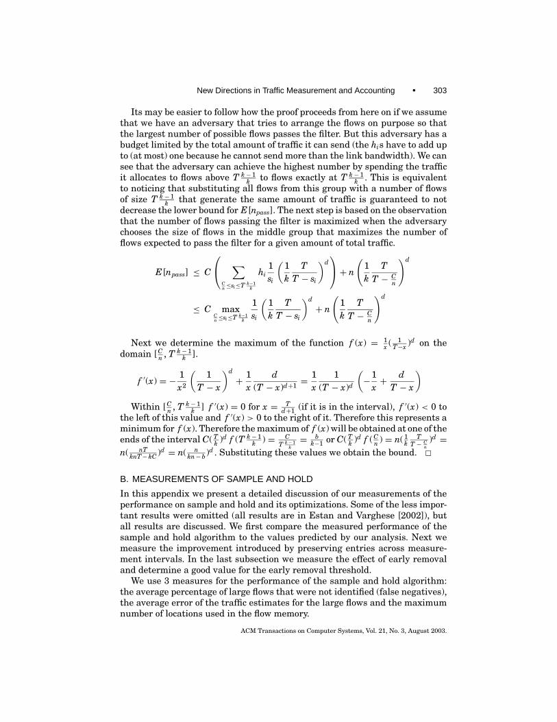
New Directions in Traffic Measurement and Accounting • 303
Its may be easier to follow how the proof proceeds from here on if we assumethat we have an adversary that tries to arrange the flows on purpose so thatthe largest number of possible flows passes the filter. But this adversary has abudget limited by the total amount of traffic it can send (the his have to add upto (at most) one because he cannot send more than the link bandwidth). We cansee that the adversary can achieve the highest number by spending the trafficit allocates to flows above T k− 1
k to flows exactly at T k− 1k . This is equivalent
to noticing that substituting all flows from this group with a number of flowsof size T k− 1
k that generate the same amount of traffic is guaranteed to notdecrease the lower bound for E[npass]. The next step is based on the observationthat the number of flows passing the filter is maximized when the adversarychooses the size of flows in the middle group that maximizes the number offlows expected to pass the filter for a given amount of total traffic.
E[npass] ≤ C
∑Cn≤si≤T k−1
k
hi1si
(1k
TT − si
)d+ n
(1k
TT − C
n
)d
≤ C maxCn≤si≤T k−1
k
1si
(1k
TT − si
)d
+ n
(1k
TT − C
n
)d
Next we determine the maximum of the function f (x) = 1x ( 1
T−x )d on thedomain [C
n , T k− 1k ].
f ′(x) = − 1x2
(1
T − x
)d
+ 1x
d(T − x)d+1 =
1x
1(T − x)d
(−1
x+ d
T − x
)Within [ C
n , T k− 1k ] f ′(x) = 0 for x = T
d+1 (if it is in the interval), f ′(x) < 0 tothe left of this value and f ′(x) > 0 to the right of it. Therefore this represents aminimum for f (x). Therefore the maximum of f (x) will be obtained at one of theends of the interval C( T
k )d f (T k− 1k ) = C
T k− 1k= b
k−1 or C( Tk )d f (C
n ) = n( 1k
TT − C
n)d =
n( nTknT− kC )d = n( n
kn− b)d . Substituting these values we obtain the bound.
B. MEASUREMENTS OF SAMPLE AND HOLD
In this appendix we present a detailed discussion of our measurements of theperformance on sample and hold and its optimizations. Some of the less impor-tant results were omitted (all results are in Estan and Varghese [2002]), butall results are discussed. We first compare the measured performance of thesample and hold algorithm to the values predicted by our analysis. Next wemeasure the improvement introduced by preserving entries across measure-ment intervals. In the last subsection we measure the effect of early removaland determine a good value for the early removal threshold.
We use 3 measures for the performance of the sample and hold algorithm:the average percentage of large flows that were not identified (false negatives),the average error of the traffic estimates for the large flows and the maximumnumber of locations used in the flow memory.
ACM Transactions on Computer Systems, Vol. 21, No. 3, August 2003.
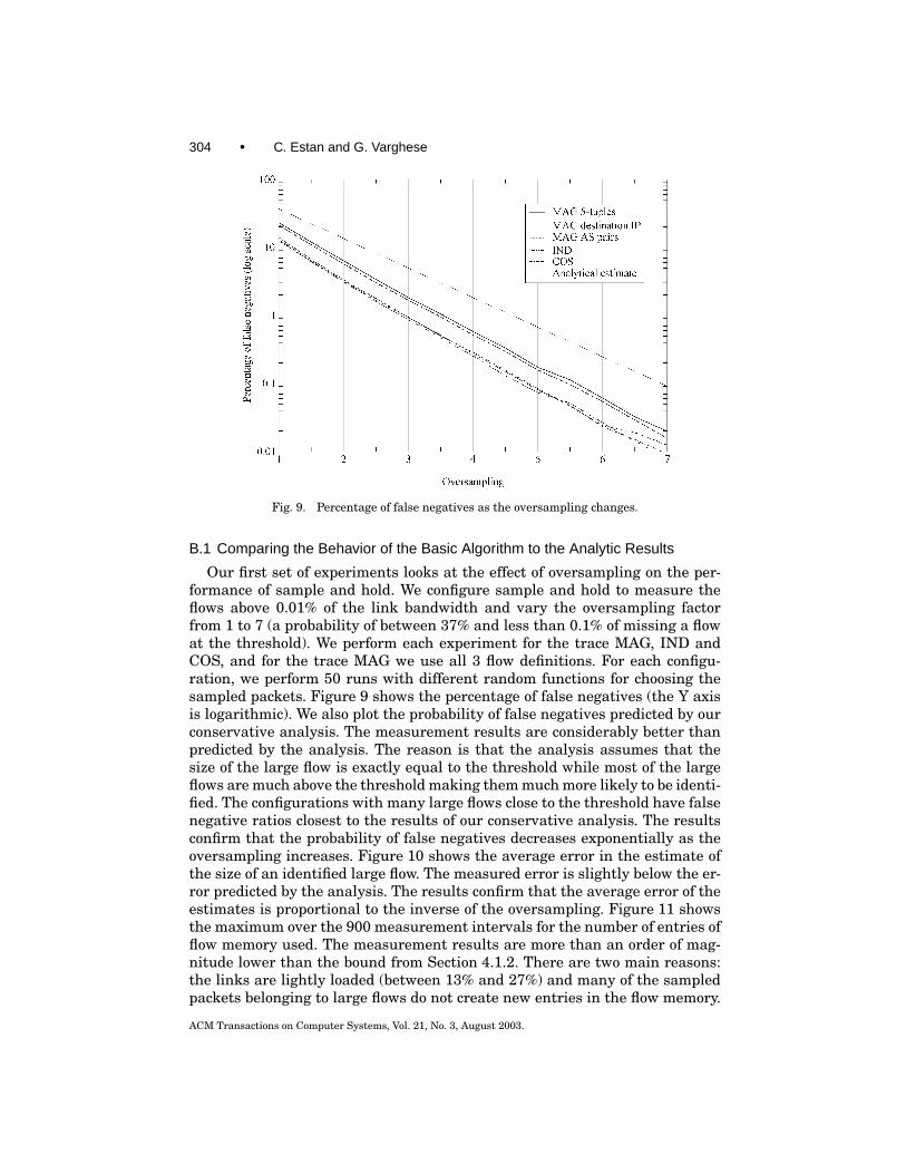
304 • C. Estan and G. Varghese
Fig. 9. Percentage of false negatives as the oversampling changes.
B.1 Comparing the Behavior of the Basic Algorithm to the Analytic Results
Our first set of experiments looks at the effect of oversampling on the per-formance of sample and hold. We configure sample and hold to measure theflows above 0.01% of the link bandwidth and vary the oversampling factorfrom 1 to 7 (a probability of between 37% and less than 0.1% of missing a flowat the threshold). We perform each experiment for the trace MAG, IND andCOS, and for the trace MAG we use all 3 flow definitions. For each configu-ration, we perform 50 runs with different random functions for choosing thesampled packets. Figure 9 shows the percentage of false negatives (the Y axisis logarithmic). We also plot the probability of false negatives predicted by ourconservative analysis. The measurement results are considerably better thanpredicted by the analysis. The reason is that the analysis assumes that thesize of the large flow is exactly equal to the threshold while most of the largeflows are much above the threshold making them much more likely to be identi-fied. The configurations with many large flows close to the threshold have falsenegative ratios closest to the results of our conservative analysis. The resultsconfirm that the probability of false negatives decreases exponentially as theoversampling increases. Figure 10 shows the average error in the estimate ofthe size of an identified large flow. The measured error is slightly below the er-ror predicted by the analysis. The results confirm that the average error of theestimates is proportional to the inverse of the oversampling. Figure 11 showsthe maximum over the 900 measurement intervals for the number of entries offlow memory used. The measurement results are more than an order of mag-nitude lower than the bound from Section 4.1.2. There are two main reasons:the links are lightly loaded (between 13% and 27%) and many of the sampledpackets belonging to large flows do not create new entries in the flow memory.
ACM Transactions on Computer Systems, Vol. 21, No. 3, August 2003.
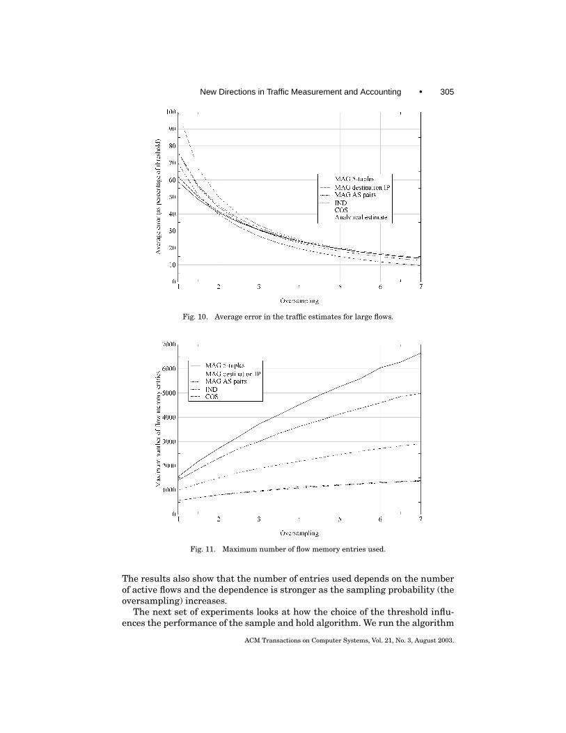
New Directions in Traffic Measurement and Accounting • 305
Fig. 10. Average error in the traffic estimates for large flows.
Fig. 11. Maximum number of flow memory entries used.
The results also show that the number of entries used depends on the numberof active flows and the dependence is stronger as the sampling probability (theoversampling) increases.
The next set of experiments looks at how the choice of the threshold influ-ences the performance of the sample and hold algorithm. We run the algorithm
ACM Transactions on Computer Systems, Vol. 21, No. 3, August 2003.
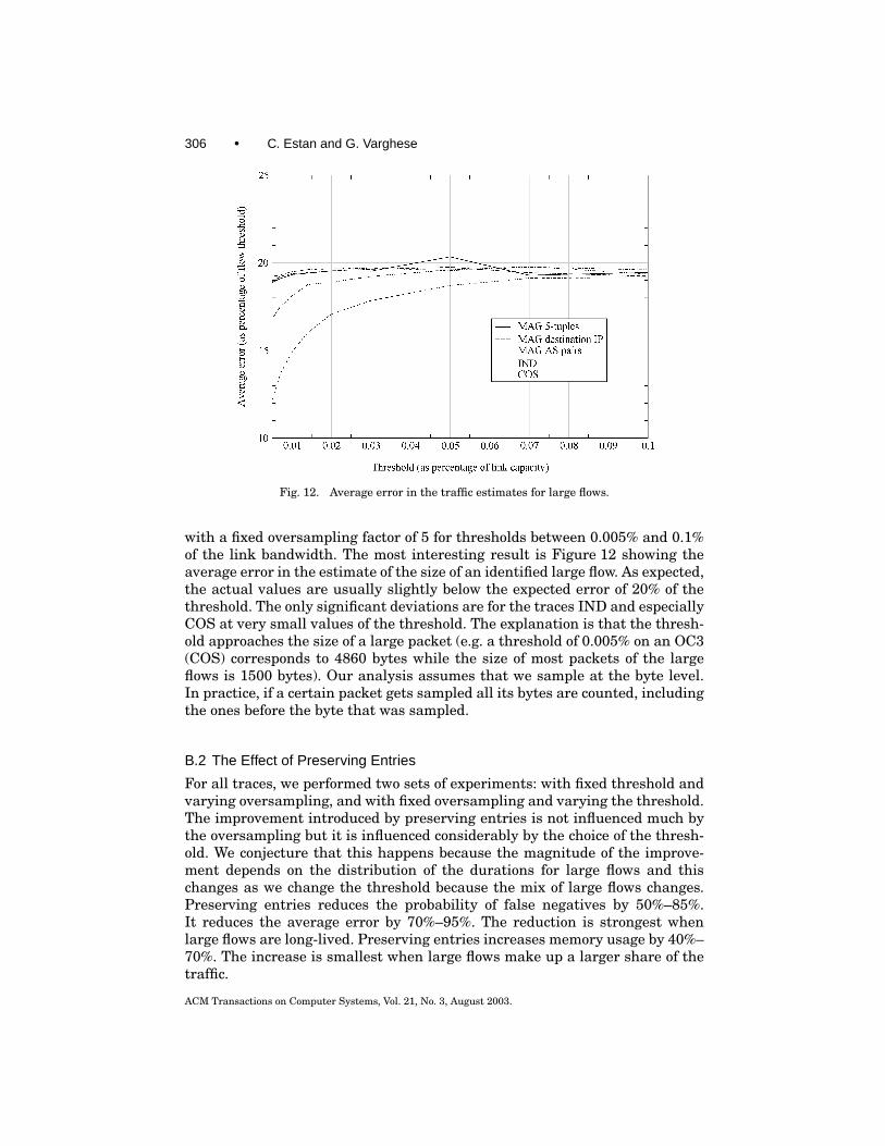
306 • C. Estan and G. Varghese
Fig. 12. Average error in the traffic estimates for large flows.
with a fixed oversampling factor of 5 for thresholds between 0.005% and 0.1%of the link bandwidth. The most interesting result is Figure 12 showing theaverage error in the estimate of the size of an identified large flow. As expected,the actual values are usually slightly below the expected error of 20% of thethreshold. The only significant deviations are for the traces IND and especiallyCOS at very small values of the threshold. The explanation is that the thresh-old approaches the size of a large packet (e.g. a threshold of 0.005% on an OC3(COS) corresponds to 4860 bytes while the size of most packets of the largeflows is 1500 bytes). Our analysis assumes that we sample at the byte level.In practice, if a certain packet gets sampled all its bytes are counted, includingthe ones before the byte that was sampled.
B.2 The Effect of Preserving Entries
For all traces, we performed two sets of experiments: with fixed threshold andvarying oversampling, and with fixed oversampling and varying the threshold.The improvement introduced by preserving entries is not influenced much bythe oversampling but it is influenced considerably by the choice of the thresh-old. We conjecture that this happens because the magnitude of the improve-ment depends on the distribution of the durations for large flows and thischanges as we change the threshold because the mix of large flows changes.Preserving entries reduces the probability of false negatives by 50%–85%.It reduces the average error by 70%–95%. The reduction is strongest whenlarge flows are long-lived. Preserving entries increases memory usage by 40%–70%. The increase is smallest when large flows make up a larger share of thetraffic.
ACM Transactions on Computer Systems, Vol. 21, No. 3, August 2003.
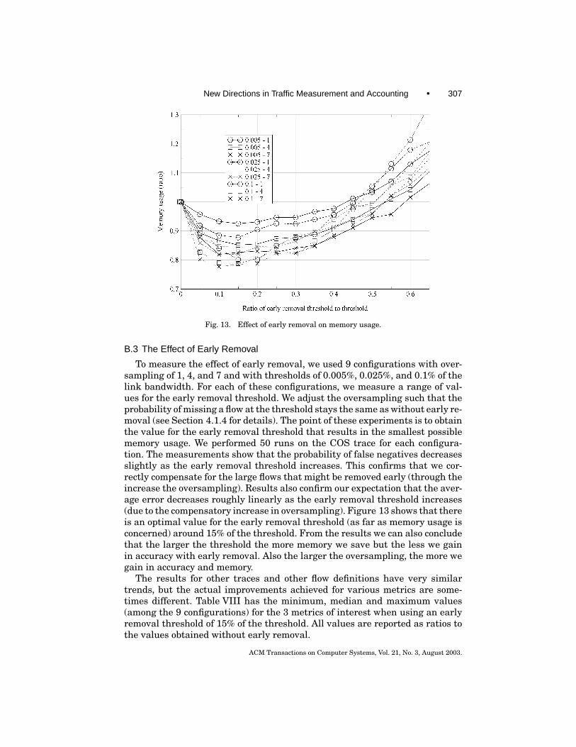
New Directions in Traffic Measurement and Accounting • 307
Fig. 13. Effect of early removal on memory usage.
B.3 The Effect of Early Removal
To measure the effect of early removal, we used 9 configurations with over-sampling of 1, 4, and 7 and with thresholds of 0.005%, 0.025%, and 0.1% of thelink bandwidth. For each of these configurations, we measure a range of val-ues for the early removal threshold. We adjust the oversampling such that theprobability of missing a flow at the threshold stays the same as without early re-moval (see Section 4.1.4 for details). The point of these experiments is to obtainthe value for the early removal threshold that results in the smallest possiblememory usage. We performed 50 runs on the COS trace for each configura-tion. The measurements show that the probability of false negatives decreasesslightly as the early removal threshold increases. This confirms that we cor-rectly compensate for the large flows that might be removed early (through theincrease the oversampling). Results also confirm our expectation that the aver-age error decreases roughly linearly as the early removal threshold increases(due to the compensatory increase in oversampling). Figure 13 shows that thereis an optimal value for the early removal threshold (as far as memory usage isconcerned) around 15% of the threshold. From the results we can also concludethat the larger the threshold the more memory we save but the less we gainin accuracy with early removal. Also the larger the oversampling, the more wegain in accuracy and memory.
The results for other traces and other flow definitions have very similartrends, but the actual improvements achieved for various metrics are some-times different. Table VIII has the minimum, median and maximum values(among the 9 configurations) for the 3 metrics of interest when using an earlyremoval threshold of 15% of the threshold. All values are reported as ratios tothe values obtained without early removal.
ACM Transactions on Computer Systems, Vol. 21, No. 3, August 2003.
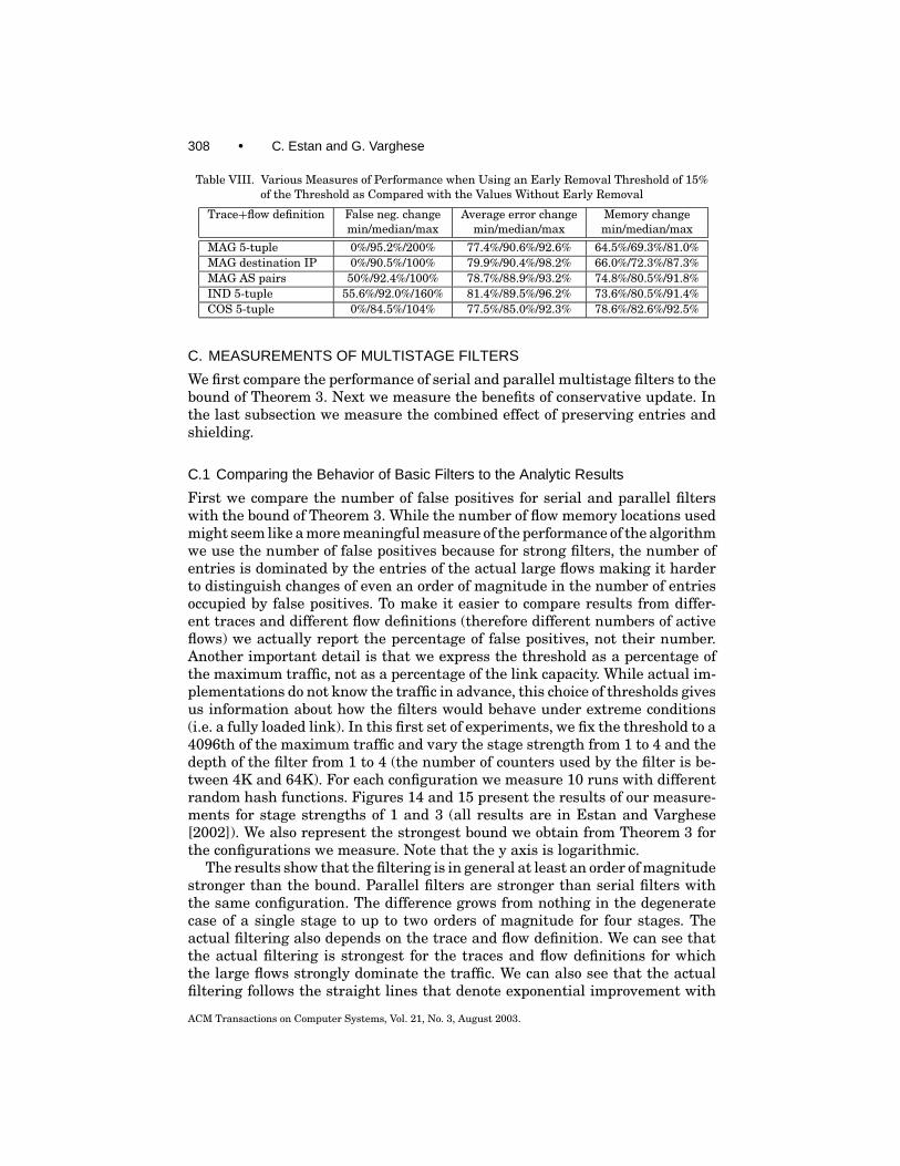
308 • C. Estan and G. Varghese
Table VIII. Various Measures of Performance when Using an Early Removal Threshold of 15%of the Threshold as Compared with the Values Without Early Removal
Trace+flow definition False neg. change Average error change Memory changemin/median/max min/median/max min/median/max
MAG 5-tuple 0%/95.2%/200% 77.4%/90.6%/92.6% 64.5%/69.3%/81.0%MAG destination IP 0%/90.5%/100% 79.9%/90.4%/98.2% 66.0%/72.3%/87.3%MAG AS pairs 50%/92.4%/100% 78.7%/88.9%/93.2% 74.8%/80.5%/91.8%IND 5-tuple 55.6%/92.0%/160% 81.4%/89.5%/96.2% 73.6%/80.5%/91.4%COS 5-tuple 0%/84.5%/104% 77.5%/85.0%/92.3% 78.6%/82.6%/92.5%
C. MEASUREMENTS OF MULTISTAGE FILTERS
We first compare the performance of serial and parallel multistage filters to thebound of Theorem 3. Next we measure the benefits of conservative update. Inthe last subsection we measure the combined effect of preserving entries andshielding.
C.1 Comparing the Behavior of Basic Filters to the Analytic Results
First we compare the number of false positives for serial and parallel filterswith the bound of Theorem 3. While the number of flow memory locations usedmight seem like a more meaningful measure of the performance of the algorithmwe use the number of false positives because for strong filters, the number ofentries is dominated by the entries of the actual large flows making it harderto distinguish changes of even an order of magnitude in the number of entriesoccupied by false positives. To make it easier to compare results from differ-ent traces and different flow definitions (therefore different numbers of activeflows) we actually report the percentage of false positives, not their number.Another important detail is that we express the threshold as a percentage ofthe maximum traffic, not as a percentage of the link capacity. While actual im-plementations do not know the traffic in advance, this choice of thresholds givesus information about how the filters would behave under extreme conditions(i.e. a fully loaded link). In this first set of experiments, we fix the threshold to a4096th of the maximum traffic and vary the stage strength from 1 to 4 and thedepth of the filter from 1 to 4 (the number of counters used by the filter is be-tween 4K and 64K). For each configuration we measure 10 runs with differentrandom hash functions. Figures 14 and 15 present the results of our measure-ments for stage strengths of 1 and 3 (all results are in Estan and Varghese[2002]). We also represent the strongest bound we obtain from Theorem 3 forthe configurations we measure. Note that the y axis is logarithmic.
The results show that the filtering is in general at least an order of magnitudestronger than the bound. Parallel filters are stronger than serial filters withthe same configuration. The difference grows from nothing in the degeneratecase of a single stage to up to two orders of magnitude for four stages. Theactual filtering also depends on the trace and flow definition. We can see thatthe actual filtering is strongest for the traces and flow definitions for whichthe large flows strongly dominate the traffic. We can also see that the actualfiltering follows the straight lines that denote exponential improvement with
ACM Transactions on Computer Systems, Vol. 21, No. 3, August 2003.
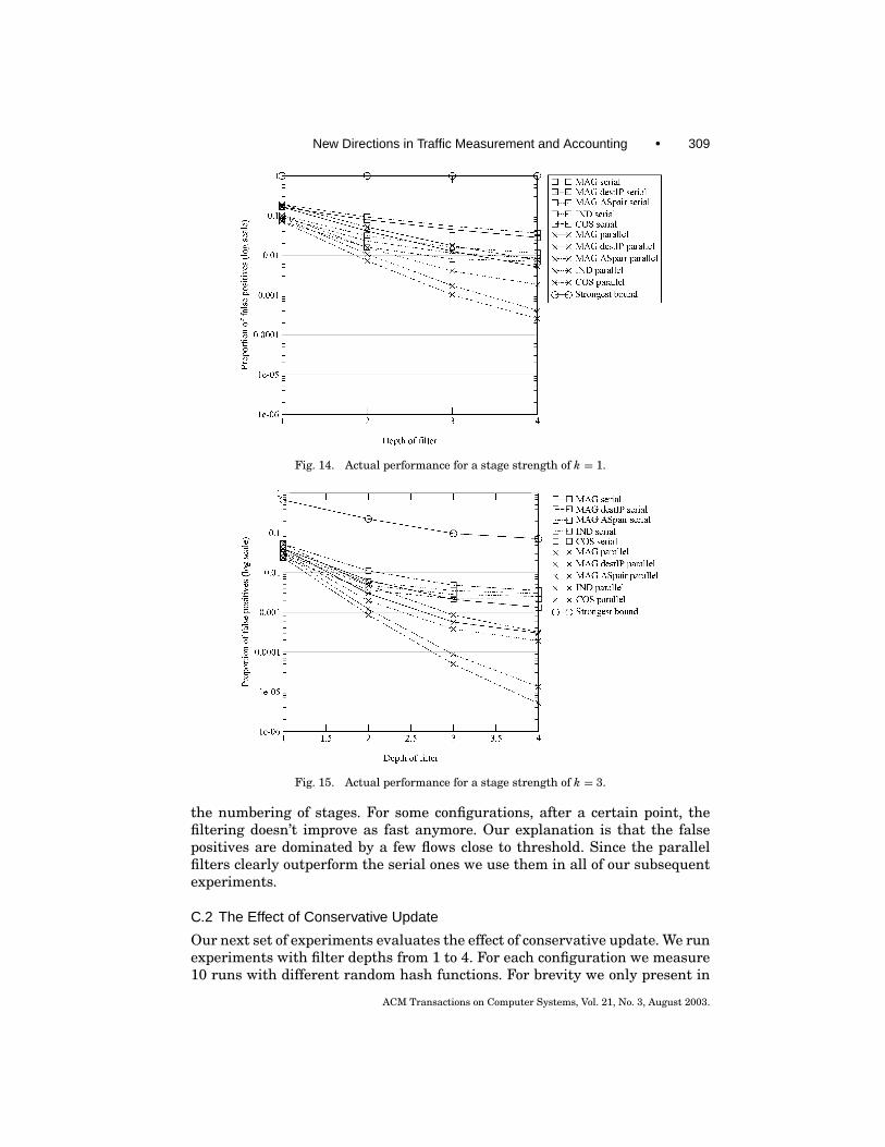
New Directions in Traffic Measurement and Accounting • 309
Fig. 14. Actual performance for a stage strength of k = 1.
Fig. 15. Actual performance for a stage strength of k = 3.
the numbering of stages. For some configurations, after a certain point, thefiltering doesn’t improve as fast anymore. Our explanation is that the falsepositives are dominated by a few flows close to threshold. Since the parallelfilters clearly outperform the serial ones we use them in all of our subsequentexperiments.
C.2 The Effect of Conservative Update
Our next set of experiments evaluates the effect of conservative update. We runexperiments with filter depths from 1 to 4. For each configuration we measure10 runs with different random hash functions. For brevity we only present in
ACM Transactions on Computer Systems, Vol. 21, No. 3, August 2003.
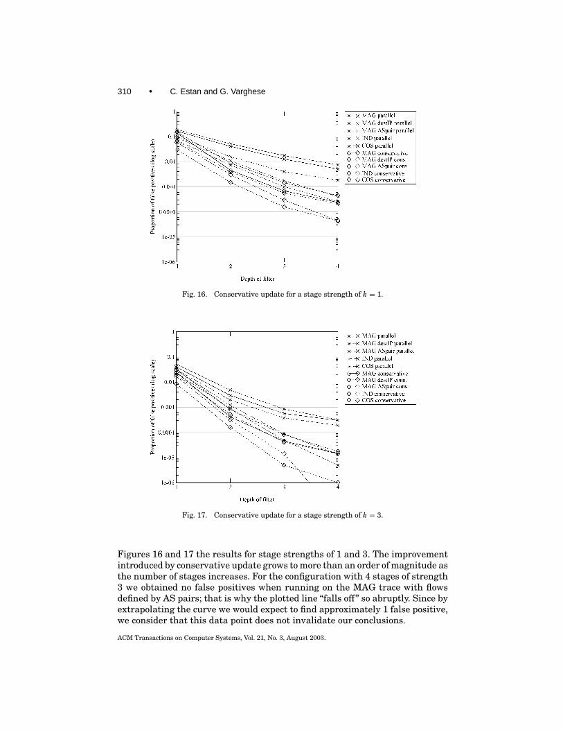
310 • C. Estan and G. Varghese
Fig. 16. Conservative update for a stage strength of k = 1.
Fig. 17. Conservative update for a stage strength of k = 3.
Figures 16 and 17 the results for stage strengths of 1 and 3. The improvementintroduced by conservative update grows to more than an order of magnitude asthe number of stages increases. For the configuration with 4 stages of strength3 we obtained no false positives when running on the MAG trace with flowsdefined by AS pairs; that is why the plotted line “falls off” so abruptly. Since byextrapolating the curve we would expect to find approximately 1 false positive,we consider that this data point does not invalidate our conclusions.
ACM Transactions on Computer Systems, Vol. 21, No. 3, August 2003.
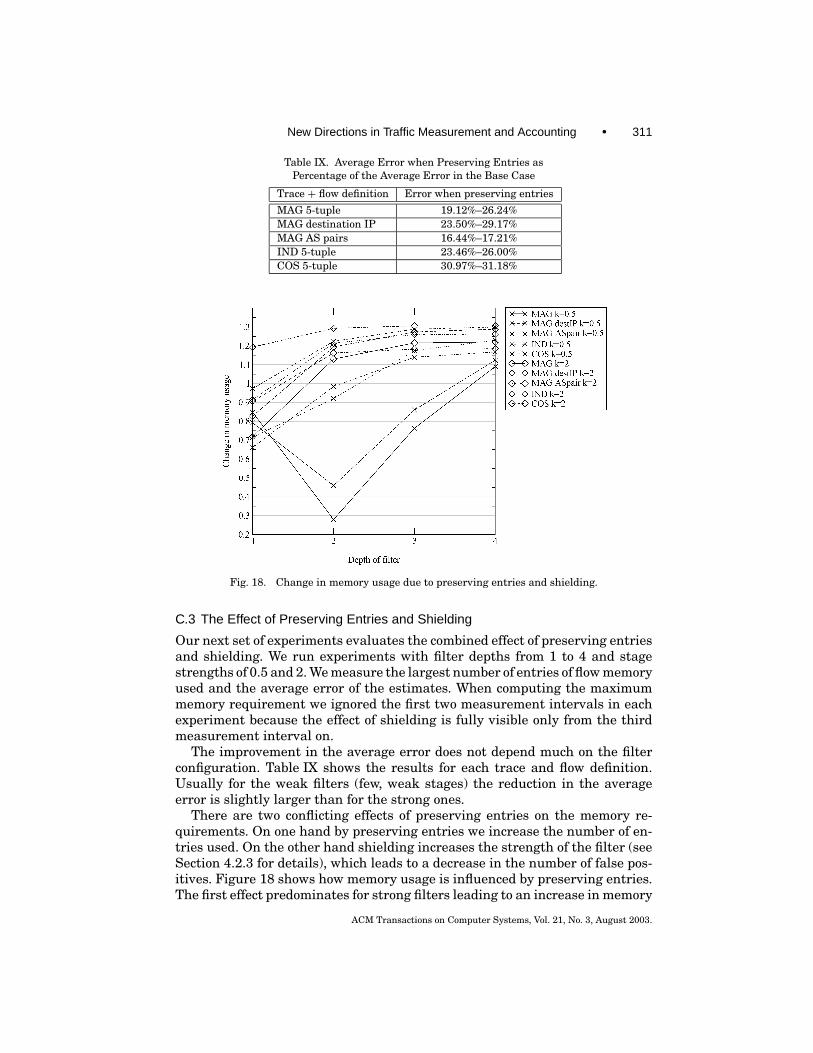
New Directions in Traffic Measurement and Accounting • 311
Table IX. Average Error when Preserving Entries asPercentage of the Average Error in the Base Case
Trace + flow definition Error when preserving entries
MAG 5-tuple 19.12%–26.24%MAG destination IP 23.50%–29.17%MAG AS pairs 16.44%–17.21%IND 5-tuple 23.46%–26.00%COS 5-tuple 30.97%–31.18%
Fig. 18. Change in memory usage due to preserving entries and shielding.
C.3 The Effect of Preserving Entries and Shielding
Our next set of experiments evaluates the combined effect of preserving entriesand shielding. We run experiments with filter depths from 1 to 4 and stagestrengths of 0.5 and 2. We measure the largest number of entries of flow memoryused and the average error of the estimates. When computing the maximummemory requirement we ignored the first two measurement intervals in eachexperiment because the effect of shielding is fully visible only from the thirdmeasurement interval on.
The improvement in the average error does not depend much on the filterconfiguration. Table IX shows the results for each trace and flow definition.Usually for the weak filters (few, weak stages) the reduction in the averageerror is slightly larger than for the strong ones.
There are two conflicting effects of preserving entries on the memory re-quirements. On one hand by preserving entries we increase the number of en-tries used. On the other hand shielding increases the strength of the filter (seeSection 4.2.3 for details), which leads to a decrease in the number of false pos-itives. Figure 18 shows how memory usage is influenced by preserving entries.The first effect predominates for strong filters leading to an increase in memory
ACM Transactions on Computer Systems, Vol. 21, No. 3, August 2003.
312 • C. Estan and G. Varghese
usage by up to 30%. The second one predominates for weak filters leading to adecrease by as much as 70%.
ACKNOWLEDGMENTS
We thank K. Claffy, D. Moore, F. Baboescu and the anonymous reviewers forvaluable comments.
REFERENCES
ALTMAN, J. AND CHU, K. 2001. A proposal for a flexible service plan that is attractive to users andinternet service providers. In IEEE Proceedings of the INFOCOM.
BLOOM, B. 1970. Space/time trade-offs in hash coding with allowable errors. Comm. ACM. 13,422–426.
BROWNLEE, N., MILLS, C., AND RUTH, G. 1999. Traffic flow measurement: Architecture. RFC 2722.BURROWS, M., ERLINGSON, U., LEUNG, S.-T., VANDEVOORDE, M., WALDSPURGER, C. A., AND WEIHL, K. W. W.
2000. Efficient and flexible value sampling. In ASPLOS.COHEN, S. AND MATIAS, Y. 2003. Spectral bloom filters. In SIGMOD/PODS.DUFFIELD, N., LUND, C., AND THORUP, M. 2001. Charging from sampled network usage. In SIG-
COMM Internet Measurement Workshop.DUFFIELD, N. G. AND GROSSGLAUSER, M. 2000. Trajectory sampling for direct traffic observation.
In Proceedings of the ACM SIGCOMM. 271–282.ESTAN, C. AND VARGHESE, G. 2002. New directions in traffic measurement and accounting. Tech.
Rep. 0699, UCSD CSE Department. Feb.FANG, M., SHIVAKUMAR, N., GARCIA-MOLINA, H., MOTWANI, R., AND ULLMAN, J. D. 1998. Computing
iceberg queries efficiently. In International Conference on Very Large Data Bases. 307–317.FANG, W. AND PETERSON, L. 1999. Inter-as traffic patterns and their implications. In Proceedings
of IEEE GLOBECOM.FELDMANN, A., GREENBERG, A., LUND, C., REINGOLD, N., REXFORD, J., AND TRUE, F. 2000. Deriving traf-
fic demands for operational ip networks: Methodology and experience. In Proceedings of the ACMSIGCOMM. 257–270.
FENG, W.-C., KANDLUR, D. D., SAHA, D., AND SHIN, K. G. 2001. Stochastic fair blue: A queue man-agement algorithm for enforcing fairness. In IEEE Proceedings of the INFOCOM.
GIBBONS, P. B. AND MATIAS, Y. 1998. New sampling-based summary statistics for improving ap-proximate query answers. In Proceedings of the ACM SIGMOD. 331–342.
HUBER, J. 2001. Design of an oc-192 flow monitoring chip. Class Project.KARP, R. M., PAPADIMITRIOU, C. H., AND SHENKER, S. 2003. A simple algorithm for finding frequent
elements in streams and bags. ACM Trans. Data. Syst.MACKIE-MASSON, J. AND VARIAN, H. 1995. Public Access to the Internet. MIT Press, Chapter Pricing
the Internet.MAHAJAN, R., BELLOVIN, S. M., FLOYD, S., IOANNIDIS, J., PAXSON, V., AND SHENKER, S. 2001. Controlling
high bandwidth aggregates in the network. http://www.aciri.org/pushback/.MOORE, D. 2001. Caida analysis of code-red. http://www.caida.org/analysis/security/code-red/.NARAYANASAMY, S., SHERWOOD, T., SAIR, S., CALDER, B., AND VARGHESE, G. 2003. Catching accurate
profiles in hardware. In HPCA.PAN, R., BRESLAU, L., PRABHAKAR, B., AND SHENKER, S. 2001. Approximate fairness through differ-
ential dropping. Tech. Rep., ACIRI.PATTERSON, D. A. AND HENNESSY, J. L. 1998. Computer Organization and Design, second ed. Morgan
Kaufmann, 619.SASTRY, S., BODIK, R., AND SMITH, J. E. 2001. Rapid profiling via stratified sampling. In 28th.
International Symposium on Computer Architecture. 278–289.SHAIKH, A., REXFORD, J., AND SHIN, K. G. 1999. Load-sensitive routing of long-lived ip flows. In
Proceedings of the ACM SIGCOMM.SHENKER, S., CLARK, D., ESTRIN, D., AND HERZOG, S. 1996. Pricing in computer networks: Reshaping
the research agenda. In ACM Comput. Comm. Rev. 26, 19–43.
ACM Transactions on Computer Systems, Vol. 21, No. 3, August 2003.
New Directions in Traffic Measurement and Accounting • 313
SMITHA, KIM, I., AND REDDY, A. L. N. 2001. Identifying long term high rate flows at a router. InProceedings of High Performance Computing.
THOMSON, K., MILLER, G. J., AND WILDER, R. 1997. Wide-area traffic patterns and characteristics.In IEEE Network.
TONG, D. AND REDDY, A. L. N. 1999. Qos enhancement with partial state. In International Work-shop on QOS.
Received July 2002; revised March 2003, April 2003; accepted April 2003
ACM Transactions on Computer Systems, Vol. 21, No. 3, August 2003.
Related Documents


