New Benders' Decomposition Approaches for W-CDMA ...

New Benders’ Decomposition Approaches

for W-CDMA Telecommunication Network

Design

by

Joe Naoum-Sawaya

A thesis

presented to the University of Waterloo

in fulfillment of the

thesis requirement for the degree of

Master of Applied Science

in

Management Sciences

Waterloo, Ontario, Canada, 2007

c©Joe Naoum-Sawaya, 2007

I hereby declare that I am the sole author of this thesis. This is a true copy of the thesis,

including any required final revisions, as accepted by my examiners.

I understand that my thesis may be made electronically available to the public.

Joe Naoum-Sawaya

ii

Abstract

Network planning is an essential phase in successfully operating state-of-the-art telecom-

munication systems. It helps carriers increase revenues by deploying the right technologies

in a cost effective manner. More importantly, through the network planning phase, carriers

determine the capital needed to build the network as well as the competitive pricing for

the offered services. Through this phase, radio tower locations are selected from a pool of

candidate locations so as to maximize the net revenue acquired from servicing a number of

subscribers. In the Universal Mobile Telecommunication System (UMTS) which is based

on the Wideband Code Division Multiple Access scheme (W-CDMA), the coverage area

of each tower, called a cell, is not only affected by the signal’s attenuation but is also af-

fected by the assignment of the users to the towers. As the number of users in the system

increases, interference levels increase and cell sizes decrease. This complicates the network

planning problem since the capacity and coverage problems cannot be solved separately.

To identify the optimal base station locations, traffic intensity and potential locations

are determined in advance, then locations of base stations are chosen so as to satisfy min-

imum geographical coverage and minimum quality of service levels imposed by licensing

agencies. This is implemented through two types of power control mechanisms. The power

based power control mechanism, which is often discussed in literature, controls the power of

the transmitted signal so that the power at the receiver exceeds a given threshold. On the

other hand, the signal-to-interference ratio (SIR) based power control mechanism controls

the power of the transmitted signal so that the ratio of the power of the received signal

over the power of the interfering signals exceeds a given threshold. Solving the SIR based

UMTS/W-CDMA network planning problem helps network providers in designing efficient

and cost effective network infrastructure. In contrast to the power based UMTS/W-CDMA

network planning problem, the solution of the SIR based model results in higher profits.

In SIR based models, the power of the transmitted signals is decreased which lowers the

interference and therefore increases the capacity of the overall network. Even though the

iii

SIR based power control mechanism is more efficient than the power based power control

mechanism, it has a more complex implementation which has gained less attention in the

network planning literature.

In this thesis, a non-linear mixed integer problem that models the SIR based power

control system is presented. The non-linear constraints are reformulated using linear ex-

pressions and the problem is exactly solved using a Benders decomposition approach. To

overcome the computational difficulties faced by Benders decomposition, two novel exten-

sions are presented. The first extension uses the analytic center cutting plane method for

the Benders master problem, in an attempt to reduce the number of times the integer

Benders master problem is solved. Additionally, we describe a heuristic that uses the an-

alytic center properties to find feasible solutions for mixed integer problems. The second

extension introduces a combinatorial Benders decomposition algorithm. This algorithm

may be used for solving mixed integer problems with binary variables. In contrast to the

classical Benders decomposition algorithm where the master problem is a mixed integer

problem and the subproblem is a linear problem, this algorithm decomposes the problem

into a mixed integer master problem and a mixed integer subproblem. The subproblem

is then decomposed using classical Benders decomposition, leading to a nested Benders

algorithm. Valid cuts are generated at the classical Benders subproblem and are added

to the combinatorial Benders master problem to enhance the performance of the algorithm.

It was found that valid cuts generated using the analytic center cutting plane method

reduce the number of times the integer Benders master problem is solved and therefore

reduce the computational time. It was also found that the combinatorial Benders reduces

the complexity of the integer master problem by reducing the number of integer variables

in it. The valid cuts generated within the nested Benders algorithm proved to be beneficial

in reducing the number of times the combinatorial Benders master problem is solved and

in reducing the computational time that the overall algorithm takes. Over 110 instances

iv

of the UMTS/W-CDMA network planning problem ranging from 20 demand points and

10 base stations to 140 demand points and 30 base stations are solved to optimality.

v

Acknowledgements

I am most grateful to my supervisor Prof. Samir Elhedhli. He introduced me to the field of

mathematical optimization when I first joined him as an undergraduate research assistant

in July 2004. His constant guidance and sharing of experience led to the success of this re-

search. I also thank him for the generous financial support through a research assistantship.

I wish to thank Prof. Khaled Soudki for giving me the possibility to visit the University

of Waterloo in July 2004. I also thank the Department of Management Sciences for the

financial assistance through the University of Waterloo International Student Award and

the University of Waterloo Merit Scholarship. I would also like to thank the faculty, staff

and students of the Department of Management Sciences for creating an enjoyable research

environment.

I would like to thank the readers of this thesis, Prof. Miguel Anjos and Prof. Moren

Levesque for their valuable comments. I also thank my friend Sami Khawam for the in-

structive discussions about the UMTS telecommunication systems.

My stay in Waterloo wouldn’t have been fruitful and enjoyable without the love, care,

and support of Bissan Ghaddar. I deeply appreciate her humor, encouragement in addition

to her technical support.

Most importantly of all, I would like to thank my father Fouad, my mother Liliane,

and my brother Hadi for the constant care, support and encouragement they provided. It

is to them that I dedicate this thesis.

vi

Contents

1 Introduction 1

1.1 Literature Review . . . . . . . . . . . . . . . . . . . . . . . . . . . . . . . . 4

1.2 Contributions of this thesis . . . . . . . . . . . . . . . . . . . . . . . . . . . 5

1.3 Structure of this thesis . . . . . . . . . . . . . . . . . . . . . . . . . . . . . 7

2 Problem Formulation and Solution Methodology 8

2.1 Problem Formulation . . . . . . . . . . . . . . . . . . . . . . . . . . . . . . 8

2.2 Linearizing Constraints (2.2) . . . . . . . . . . . . . . . . . . . . . . . . . . 12

2.3 Benders Decomposition . . . . . . . . . . . . . . . . . . . . . . . . . . . . . 13

2.4 Solving the UMTS/W-CDMA network planning problem . . . . . . . . . . 15

3 Accelerating Benders Decomposition using Central Cuts 20

3.1 Literature Review . . . . . . . . . . . . . . . . . . . . . . . . . . . . . . . . 20

3.2 ACCPM . . . . . . . . . . . . . . . . . . . . . . . . . . . . . . . . . . . . . 22

3.2.1 Integer Analytic Centers . . . . . . . . . . . . . . . . . . . . . . . . 24

3.3 A Two-Phase ACCPM Algorithm . . . . . . . . . . . . . . . . . . . . . . . 25

3.4 Solving the UMTS/W-CDMA network planning problem . . . . . . . . . . 27

3.4.1 Heuristics for finding the IP analytic center . . . . . . . . . . . . . 31

3.5 Computational Results . . . . . . . . . . . . . . . . . . . . . . . . . . . . . 36

vii

4 Nested and Combinatorial Benders Decomposition Algorithms 48

4.1 Combinatorial Benders Decomposition Algorithm . . . . . . . . . . . . . . 49

4.1.1 Ensuring a bounded [MP] formulation . . . . . . . . . . . . . . . . 51

4.1.2 Avoiding Total Enumeration . . . . . . . . . . . . . . . . . . . . . . 52

4.2 Nested Benders Decomposition . . . . . . . . . . . . . . . . . . . . . . . . 53

4.3 Valid Inequalities . . . . . . . . . . . . . . . . . . . . . . . . . . . . . . . . 61

4.4 Computational Results . . . . . . . . . . . . . . . . . . . . . . . . . . . . . 68

5 Conclusion 73

viii

List of Tables

3.1 Data for the test cases . . . . . . . . . . . . . . . . . . . . . . . . . . . . . 37

3.2 Computational Results - Classical Benders Decomposition . . . . . . . . . 38

3.3 Computational Results - Two-phase ACCPM Algorithm . . . . . . . . . . 38

3.4 Computational Results - Two-phase Algo. - Weight on Constraints set to 1 40

3.5 Computational Results - Two-phase Algorithm - Kelley Based . . . . . . . 41

3.6 Computational Results - Two-phase ACCPM Algo. - Rounding Heuristic 1 42





4.1 Example of the search algorithm for finding valid inequalities . . . . . . . . 67

4.2 Computational Results - Nested Benders Decomposition . . . . . . . . . . 70



ix

List of Figures

2.1 A UMTS Network. . . . . . . . . . . . . . . . . . . . . . . . . . . . . . . . 9

3.1 Analytic center cutting plane method. . . . . . . . . . . . . . . . . . . . . 23

3.2 Central Rounding Heuristic . . . . . . . . . . . . . . . . . . . . . . . . . . 33

3.3 Number of times the IP master problem is solved. . . . . . . . . . . . . . . 45

3.4 Total CPU time consumed by each algorithm . . . . . . . . . . . . . . . . 46

4.1 Nested Benders Decomposition. . . . . . . . . . . . . . . . . . . . . . . . . 57

4.2 Nested Benders Decomposition Flowchart. . . . . . . . . . . . . . . . . . . 60

x

Chapter 1

Introduction

Universal Mobile Telecommunication Systems (UMTS) are the third generation of wire-

less cellular network standards. A major contribution of UMTS networks is the use of

Wideband Code Division Multiple Access (W-CDMA) radio transmission technology, that

represents a major evolution in offering a wide range of applications that require high data

rates. For instance, mobiles can theoretically be allocated connections up to 2Mbps data

rates. The shift towards the use of UMTS networks is motivated by its ability to offer end

user applications at low costs. By the last quarter of 2006, UMTS subscriptions reached

100 million worldwide with a growth of 3 million new subscribers each month. Japan, the

first country to deploy UMTS networks in 2001, offers the service for 30 million subscribers.

Most European countries started to adopt UMTS technology in 2002. By the end of 2006,

the number of UMTS subscribers in Europe reached 40 million. While currently UMTS

is implemented in 130 networks in more than 50 countries, most cellular operators are

expected to implement UMTS systems as part of their networks by 2007 (UMTS Forum

White Paper, 2006).

A critical aspect of UMTS deployment is Radio Network Planning, which seeks to de-

termine the location of transmitters for a certain area with specific traffic demand and

1

propagation gains so as to minimize the cost of network deployment and operation. Simi-

lar problems have been discussed for the first and second generations of cellular networks.

Typically, the service area is broken to several radio cells each served by a single transmit-

ter known as a base station. Each base station communicates to mobiles by transmitting

a radio signal, thus causing interference to other base stations.

In first generation cellular networks, mobiles differentiate between their own transmit-

ters and interfering transmitters by assigning different frequencies for each cell. This is

known as frequency division multiple access (FDMA). Frequencies may be reused by differ-

ent cells since signal power depletes with distance, thus similar frequencies may be assigned

to different cells separated by a large enough distance. Models and algorithms for FDMA

networks are discussed in Koster (1999). An extensive survey for frequency assignment in

FDMA networks is provided in Murphey et al. (1999).

In second generation cellular networks each frequency channel is shared among differ-

ent users by dividing it into time slots. This is known as time division multiple access

(TDMA). These networks are modeled and solved as coverage problems in Hao et al.

(1997), Molina et al. (1999) and Mathar and Niessen (2000). Global System for Mo-

bile Communication (GSM) combines TDMA and FDMA to divide a 25 MHZ band-

width among 124 carrier frequencies each divided into eight time slots. As discussed in

Naghshineh and Katzela (1996) and Berruto et al. (1998), the combination of TDMA and

FDMA separates the network planning problem into two phases. The first phase identifies

the locations of base stations taking into account signal propagation and system capacities,

while the second phase distributes the frequencies to the base stations, as done in FDMA

networks. Alternatively, instead of dividing a channel to frequencies as in FDMA or to time

slots as in TDMA, code division multiple access (CDMA) encodes the data transmitted on

each channel by a specific code thus allowing the receiver to differentiate between data sig-

nals and interfering signals. W-CDMA upgrades CDMA to include multiple features such

2

as frequency and time division duplex modes (FDD and TDD), as well as adaptive power

control based on signal to interference ratios (SIR). UMTS is built on second generation

infrastructures and mainly GSM infrastructure to include W-CDMA features.

Even though UMTS and GSM are built on similar infrastructures, network planning

techniques adopted in GSM are not appropriate to UMTS network planning. The liter-

ature discussing GSM network planning proposes two solution models. The first one is

a coverage problem where base stations are identified, with the objective of maximizing

signal levels in selected areas. Propagation models such as the Hata Model (Hata, 1980)

are often used to identify the constraints. The second is a frequency assignment problem

where for each base station, a frequency is selected from a pool of frequencies with the

objective of minimizing interference levels. Techniques adopted by GSM network plan-

ning are not appropriate for UMTS network planning due to a number of fundamental

differences between the two standards. In UMTS, base stations’ coverage areas, i.e. cell

sizes, are not static but rather dependent on the amount of served traffic. For instance a

phenomenon, known as “Cell Breathing Effect” occurs as traffic load changes in a cell. Cell

size decreases as traffic load increases whereas it increases as traffic load decreases. This

dynamic behavior of cell areas does not allow the use of coverage problems similar to those

used in GSM. Another fundamental difference between GSM and UMTS is that bandwidth

in UMTS is shared among all base stations (frequency reuse factor equal to one), thus no

frequency assignment problem exists for such networks. UMTS network planning should

not be based on coverage but also on interference levels. Interference is dependent on the

power emitted by each mobile station and controlled by power control mechanisms. Signal

to Interference Ratio (SIR) is used as an interference level indicator. In contrast to GSM

where different frequencies are used to eliminate interference, UMTS utilizes spread spec-

trum where each signal is spread using a pseudo random spreading code. Using spreading

codes, the power of the interference is reduced by a spreading factor (SF). Spreading codes

are mutually orthogonal hence decoding at receivers allows the distinction between the

3

interfering signals.

1.1 Literature Review

Several papers discuss network planning for third generation networks. Tutschku (1998)

models network planning as a supply chain where demand point are modeled as customers

with stochastic independent demands. The problem is then reduced to finding the mini-

mum number of base stations that can cover all demand points taking into account that

each demand point is covered by at least a single base station. This approach may not

accurately model UMTS systems since demands are not independent (i.e. SIR for each

connection is dependent on the number of other connections.). In Lee and Kang (2000),

a similar modeling scheme is adopted and the resulting problem is solved by a tabu search

algorithm. A different objective is provided in Sherali et al. (1996) where base stations are

located so as to minimize power loss (i.e minimize distance) between the base stations and

the demand points.

Recent literature models SIR constraints explicitly. In particular in Galota et al. (2001),

SIR is considered however intercell interference is neglected and only intracell interference

is modeled. Amaldi et al. (2002) model intracell interference as a fraction of intercell

interference and prove that the SIR constraint will then constitute a maximum cell capacity.

Additionally, Amaldi et al. (2002) and Amaldi et al. (2003) distinguish between two UMTS

network planning models. These models differ in the power control (PC) mechanism which

is used to adjust the power of the transmitted signals. Two PC mechanisms are discussed:

In the power based PC mechanism, signals are transmitted with a high enough power

so that the power of the received signal exceeds a given threshold value. In the SIR

based PC mechanism, signals are transmitted with a high enough power so that the SIR

of the received signal exceeds a given threshold value. Power control minimizes power

consumption and reduces interference by keeping the power of the transmitted signals

4

high enough to guarantee signal quality requirements, and low enough so as to minimize

interference with other signals. Due its complexity, the SIR based PC mechanism has

gained less attention within the scope of network planning literature. In contrast, the

power based PC mechanism provides less complex models, however resulting network plans

are allocated more resources than required by networks operating under SIR based PC.

Amaldi et al. (2003) show that the SIR based PC model provides more efficient plans

compared to the power based PC model. Furthermore, the computed SIR levels are closer

to the actual values of real systems. A tabu search algorithm is used in Amaldi et al. (2003)

to find feasible solutions for the two models. An evaluation of the discussed power control

mechanisms may be found in Yates (1995). Recent work of Kalvenes et al. (2006) builds

on the work of Amaldi et al. (2003) and solves the power based PC model in Cplex using

a priority branching algorithm. Even though this paper provides solutions with a gap of

less than 10% from the optimal solution, no discussion is provided for the SIR based power

control mechanism. Olinick and Rosenberger (2002) extend the work of Kalvenes et al.

(2002) and solve a stochastic model for the power based power control problem. Based

on the stochastic model, Olinick and Rosenberger (2002) state that the SIR based power

control is non-linear and “an exact solution procedure appears to be beyond the capabilities

of the current state-of-the art of mathematical programming techniques”.

1.2 Contributions of this thesis

In this thesis, a profit maximization model for the SIR based power control system is pre-

sented and solved. In contrast to the power based UMTS/W-CDMA network planning

problem which is often discussed in literature, solving the SIR based model results in more

efficient network plans. In SIR based models, the power of the transmitted signals is de-

creased which lowers the interference and therefore increases the capacity of the overall

network.

5

The presented SIR based model contains non-linear constraints. These constraints are

reformulated using linear expressions and the model is exactly solved using a Benders De-

composition approach. To enhance Benders decomposition, two approaches that aim at

accelerating the algorithm are presented and evaluated. The first extension uses the ana-

lytic center cutting plane method (ACCPM) to generate valid cuts that aim at reducing

the number of times the integer Benders master problem is solved. This is done using a

two-phase ACCPM algorithm. In the first phase, the linear (LP) relaxation of the problem

is solved using the analytic center cutting plane algorithm in a Benders decomposition

framework. This generates a set of valid cuts that are added to the original problem which

is solved in phase II using the classical Benders approach. The valid cuts reduce the num-

ber of times the integer Benders master problem is solved, and therefore reduce the total

computational time. Within the scope of the two-phase ACCPM algorithm, a heuristic

that uses the analytic center properties to find feasible solutions of general mixed integer

problems is discussed. This work is first to use ACCPM in this fashion and can be applied

to general mixed integer problems.

As a second approach, a nested Benders decomposition algorithm is introduced where a

classical Benders algorithm is used within a combinatorial Benders algorithm. Combinato-

rial Benders decomposition is used to solve mixed integer problems with binary variables.

In contrast to the classical Benders decomposition algorithm where the problem is de-

composed into a mixed integer master problem and a linear subproblem, this algorithm

decomposes the problem into a mixed integer master problem and a mixed integer sub-

problem. This aims at reducing the complexity of the master problem by reducing the

number of integer variables in it. This approach reduces the computational burden of

solving hard integer Benders master problems. In addition, we propose a set of valid cuts

that are generated at the classical Benders subproblem and are valid to the combinatorial

Benders master problem.

6

This thesis contributes to the solvability of the profit maximization SIR based UMTS/W-

CDMA network planning problem as well as of general mixed integer programs. Two novel

algorithmic ideas are used. First, an ACCPM-based Benders decomposition is proposed.

Second, a nested combinatorial/classical Benders decomposition is explored, enhanced us-

ing valid cuts, and tested. The UMTS/W-CDMA network planning problem is solved

using the proposed algorithms. Problems of up to 140 demand points and 30 potential

base station locations are solved to optimality within 10 minutes using the nested Ben-

ders algorithm. The ACCPM-based Benders algorithm was found to reduce the number

of integer master problems solved. The proposed solution methodologies were efficient in

solving the UMTS/W-CDMA network planning problem. Furthermore, the nested Ben-

ders decomposition and the two-phase ACCPM algorithms are general and can be applied

to solve scheduling, location optimization and assignment problems.

1.3 Structure of this thesis

Following this introductory chapter, Chapter 2 presents the model formulation of the

UMTS/W-CDMA network planning problem and describes the classical Benders decom-

position algorithm. In Chapter 3, the analytic center cutting plane method (ACCPM) and

its extension to Benders decomposition are discussed. Chapter 4 introduces the Combina-

torial Benders decomposition and its extension to Nested Benders decomposition. Finally,

Chapter 5 concludes this work.

7

Chapter 2

Problem Formulation and Solution

Methodology

2.1 Problem Formulation

Given a set of I demand points (DP) DP1, . . . , DPI where at each DPi, Ui stochastic and

independent number of simultaneous connections are anticipated; and a set of J potential

base station (BS) locations BS1, . . . , BSJ , the UMTS/W-CDMA network planning prob-

lem seeks to determine the location of the base stations and the assignment of the demand

points to base stations so as to maximize the profit acquired from servicing a number of

users. A fixed profit ri is generated from each serviced user at location DPi, i = 1, . . . , I.

Each base station location is associated with a cost cj that includes the cost of building and

operating a base station at location BSj, j = 1, . . . , J . A fixed cost λ is associated with

power transmission. The power of the signal transmitted between DPi and BSj attenuates

due to many factors such as distance, obstacles, and antenna setup. These factors are

captured by a propagation gain factor which is dependent on BS location relative to each

DP. For each link between DPi and BSj, a power gain factor gij is defined. The UMTS

network setup is shown in Figure 2.1.

8

Figure 2.1: A UMTS Network.

9

We define the following decision variables:

yj =

1 if BSj location is selected

0 otherwise

xij =

1 if DPi is linked to BSj

0 otherwise

zi =

1 if DPi is linked to at least one base station

0 otherwise

pi: the power transmitted by each mobile station at DPi

The presented model considers a SIR based PC mechanism. Parameter SIRmin specifies

the target SIR level required for each signal. Therefore, given a connection between DPi

and BSj, SIRij ≥ SIRmin should be satisfied. The SIR is given by the following equation:

SIR = SFPreceived

αIin + Iout + η,

where Preceived is the power of the received signal which is a factor of the transmitted

power. Power loss is incurred due to environment and may be estimated using propagation

models such as the Hata Model (Hata, 1980), and the 2 ray Model (Parsons, 1996). Iin is

the power of interfering signals transmitted by the same BS (Intracell Interference), and

Iout is the power of interfering signals transmitted by other BSs (Intercell Interference). η

is the receiver thermal noise and 0 ≤ α ≤ 1 is the orthogonality loss factor. We assume

that the number of spreading codes is higher than the number of available connections

therefore we may consider α = 1. We can safely take this assumption in the uplink

direction (i.e. connection from DP to BS) since there would exist a very large number of

10

orthogonal spreading codes. The power of the interference is reduced by a spreading factor

(SF ). Additional details are presented in Kim and Jeong (2000). Suppose a connection

is established between a mobile station at location DPi and a tower at location BSj, a

mobile station at DPi transmits signals at a given power pi. Due to signal attenuation, it is

received by BSj at a power Preceived = gijpi. At the same location DPi, Ui−1 other mobile

stations are interfering at a power pi each and received at BSj with a power (Ui − 1)gijpi.

At each demand point location DPk 6=i, Uk mobile stations are transmitting at a power pk

each, and received at a power Ukgkjpk. The total interference is∑

k 6=i Ukgkjpk. Therefore,

the SIR constraint can be formulated as:

SFpigij

(Ui − 1)pigij +∑

k 6=i Ukgkjpk + η≥ SIRminxij ∀i ∈ I, ∀j ∈ J.

This constraint is redundant when xij = 0, otherwise when xij = 1 the SIR constraint is

enforced. The UMTS/W-CDMA network planning problem is now formulated as follows:

[OP ] :maxI∑

i=1

riUizi −J∑

j=1

cjyj − λI∑

i=1

Uipi

s.t. xij − yj ≤ 0 ∀i ∈ I, ∀j ∈ J, (2.1)

SFpigij


k 6=i Ukgkjpk + η≥ SIRminxij ∀i ∈ I, ∀j ∈ J, (2.2)

zi −J∑j

xij ≤ 0 ∀i ∈ I, (2.3)

I∑i

Uizi ≥ π

I∑i

Ui, (2.4)

0 ≤ pi ≤ pmax ∀i ∈ I, (2.5)

zi, yj, xij ∈ {0, 1}.

Note that constraints (2.2) are non-linear. The objective maximizes the profit generated

by the network. In contrast to the model provided in Kalvenes et al. (2006), we include

the power cost in the objective function. Even though this complicates the model, it

11

ensures that the optimal network plan guarantees the use of the lowest possible power

levels. Constraint (2.1) ensures that DPi cannot be linked to BSj unless BSj is selected.

Constraint (2.2) ensures that a link between DPi and BSj is not valid unless it satisfies

the minimum SIR condition SIRij > SIRmin. Constraints (2.3) and (2.4) ensure that at

least π percent of the DP locations are covered. Parameter π is often imposed by agencies

that regulate radio communication in concerned areas. Constraint (2.5) ensures that the

power at which each DP is transmitting does not exceed a maximum of pmax.

2.2 Linearizing Constraints (2.2)

Constraints (2.2) are conditional non-linear constraints of the form

if xij = 1 then SFpigij


k 6=i Ukgkjpk + η≥ SIRmin.

This constraint may be linearized through a big-M coefficient Mij as follows.

SFpigij − [(Ui − 1)pigij +∑k 6=i

Ukgkjpk + η]SIRmin ≥ (xij − 1)Mij. (2.6)

The use of big-M is often not desirable. As discussed later, Benders decomposition elimi-

nates the big-M coefficient from constraints (2.2) in the subproblem, however the resulting

Benders cuts still depend on the big-M values. Choosing a sufficiently large big-M constant

in a mixed integer problem affects the LP relaxation. In fact the strongest LP relaxation

will result from choosing the smallest possible big-M value. In equation (2.6), a good value

for the big-M may be selected as follows:

If SFpigij > (Ui − 1)pigijSIRmin i.e. SF > (Ui − 1)SIRmin,

SFpigij − [(Ui − 1)pigij +∑

k 6=i Ukgkjpk + η]SIRmin attains its minimum at pi = 0 and

pk = pmax ∀k 6= i. Thus, a good value for Mij would be (∑

k 6=i Ukgkjpmax + η)SIRmin.

If SFpigij < (Ui − 1)pigijSIRmin i.e. SF < (Ui − 1)SIRmin,

12

SFpigij − [(Ui − 1)pigij +∑

k 6=i Ukgkjpk + η]SIRmin attains its minimum at pi = pmax ∀i.Thus, a good value for Mij is −SFpmaxgij +[(Ui−1)pmaxgij +

∑k 6=i Ukgkjpmax +η]SIRmin.

In the following section, we provide an exposition of Benders decomposition. Details on

applying Benders decomposition to solve the UMTS/W-CDMA network planning problem

are then provided.

2.3 Benders Decomposition

A number of optimization problems take the following general structure:

min cT x + dT y

s.t. A1y ≤ b1, (2.7)

A2x + My ≥ b2, (2.8)

y ≥ 0 and integer, (2.9)

x ≥ 0, (2.10)

which can be exploited through Benders decomposition (Benders, 1962; Geoffrion, 1972).

By projecting problem (2.7)-(2.10) on the space defined by the y variables only, the resulting

problem is:

min dT y + min{cT x|A2x ≥ b2 −My, x ≥ 0}

s.t. A1y ≤ b1, (2.11)

y ≥ 0 and integer.

The inner minimization problem is rewritten as the dual maximization problem as follows:

max (b2 −My)λ

s.t. AT2 λ ≤ c,

λ ≥ 0.

13

Let HP and HR be the sets of extreme points and extreme rays of the set {λ|AT2 λ ≤ c, λ ≥

0}. The problem formulated in (2.11) is equivalent to

min dT y + θ

s.t. A1y ≤ b1, (2.12)

(b2 −My)λ ≤ θ λ ∈ HP , (2.13)

(b2 −My)µ ≤ 0 µ ∈ HR, (2.14)

y ≥ 0 and integer. (2.15)

Starting with an initial empty set of extreme rays and extreme points, the cutting plane

algorithm solves the relaxed IP master problem

min dT y

s.t. A1y ≤ b1,

y ≥ 0 and integer.

With fixed y values (obtained from the relaxed master problem), optimality cuts are gen-

erated from the extreme points of the subproblem. This can be done by solving the primal

subproblem

min cT x

s.t. A2x ≥ b2 −My,

x ≥ 0,

or equivalently, its dual

max (b2 −My)λ

s.t. AT2 λ ≤ c, (2.16)

λ ≥ 0.

14

If the primal subproblem is infeasible or equivalently the dual subproblem is unbounded,

then a feasibility cut is generated from the dual extreme ray of unboundedness. This can

be found by solving the auxiliary subproblem (see Bazaraa and Jarvis, 1977)

max 0

s.t. (b2 −My)λ = 1, (2.17)

AT2 λ ≤ 0, (2.18)

λ ≥ 0.

Generated cuts are appended to the master problem and the algorithm reiterates until an

optimal solution is found.

2.4 Solving the UMTS/W-CDMA network planning

problem using Benders Decomposition

The formulation of the UMTS base station location optimization problem presented in

(2.1) - (2.5) falls within the generic structure of problem (2.7)-(2.10). As described earlier,

this structure can be exploited using Benders decomposition. In particular, the fact that

the problem presented in (2.1) - (2.5) in the x, y, and z variables alone is relatively easy to

solve, motivates the use of Benders decomposition.

For fixed xij, yj, and zi, problem [OP] reduces to the primal subproblem:

[PSP]: ZPSP = minI∑i

Uipi

s.t. pi ≤ pmax ∀i, (2.19)


Ukgkjpk + η]SIRmin ≥ (xij − 1)Mij ∀i,∀j, (2.20)

pi ≥ 0 ∀i, (2.21)

15

whose dual is:

[DSP]: ZDSP = max pmax

I∑i

αi +I∑i

J∑j

[(xij − 1)Mij + ηSIRmin]βij

s.t. αi +J∑j

βij(SFgij − (Ui − 1)gijSIRmin)− SIRmin

∑k 6=i

∑j

Ukgkjβkj ≤ Ui ∀i,

αi ≤ 0, βij ≥ 0 ∀i,∀j,

which is equivalent to:

ZDSP = maxh∈HP

{pmax

I∑i

αhi +

I∑i

J∑j

[(xij − 1)Mij + ηSIRmin]βhij}

where [αhi , β

hij], h ∈ HP , are the extreme points of the set:

U =

{(α, β) : αi +

∑j βij(SFgij − (Ui − 1)gijSIRmin)− SIRmin

∑k 6=i

∑j Ukgkjβkj ≤ Ui ∀i

αi ≤ 0, βij ≥ 0 ∀i,∀j

}.

If the set U is bounded, we generate an optimality cut of the form

θ −I∑i

J∑j

Mijβhijxij ≥ pmax

I∑i

αhi +

I∑i

J∑j

(ηSIRmin −Mij)βhij, h ∈ HP (2.22)

where αhi and βh

ij are the extreme points of [DSP].

If U is unbounded, we generate a feasibility cut of the form

−I∑i

J∑j


I∑i

αhi +

I∑i

J∑j

(ηSIRmin −Mij)βhij, h ∈ HR (2.23)

where αhi and βh

ij are the extreme rays of [DSP].

The values of αhi and βh

ij of the extreme ray are generated by solving the auxiliary sub-

16

problem

[ASP]: max 0

s.t. pmax

I∑i

αi +I∑i

J∑j

[(xij − 1)Mij + ηSIRmin]βij = 1,

αi +J∑j


∑k 6=i

∑j

Ukgkjβkj ≤ 0 ∀i,

αi ≤ 0, βij ≥ 0 ∀i, ∀j.

Note that since xij is fixed in the subproblem, constraint (2.20) may be linearized as follows:

pi(SFgij − (Ui − 1)gijSIRminxij)− SIRminxij

∑k 6=i

Ukgkjpk ≥ ηSIRminxij ∀i,∀j (2.24)

Replacing equation (2.20) by equation (2.24), the primal subproblem can be rewritten as:

[PSP]: minI∑i

Uipi

s.t. pi ≤ pmax ∀i,

pi(SFgij − (Ui − 1)gijSIRminxij)− SIRminxij

∑k 6=i

Ukgkjpk ≥ ηSIRminxij ∀i,∀j,

pi ≥ 0 ∀i,

whose dual is:

[DSP]: max pmax

I∑i

αi +I∑i

J∑j

ηSIRminxijβij

s.t. αi +J∑j

βij(SFgij − (Ui − 1)gijSIRminxij)− SIRmin

∑k 6=i

∑j

Ukgkjxijβkj ≤ Ui ∀i,

(2.25)

αi ≤ 0, βij ≥ 0 ∀i,∀j, (2.26)

17

and the auxiliary subproblem is:

[ASP]: max 0

s.t. pmax

I∑i

αi +I∑i

J∑j

ηSIRminxijβij = 1,

αi +J∑j


∑k 6=i

∑j

Ukgkjβkj ≤ 0 ∀i,

αi ≤ 0, βij ≥ 0 ∀i, ∀j.

Note that the new [PSP], [DSP] and [ASP] formulations do not depend on the big-M. This

eliminates any computational complexities resulting from the use of large big-M values at

the level of the subproblem.

The Benders master problem is:

[MP] := maxI∑i

riUizi −J∑j

cjyj − λθ

s.t. θ −I∑i

J∑j


I∑i

αhi +

I∑i

J∑j

(ηSIRmin −Mij)βhij ∀h ∈ HP (2.27)

−I∑i

J∑j


I∑i

αhi +

I∑i

J∑j

(ηSIRmin −Mij)βhij ∀h ∈ HR (2.28)

xij − yj ≤ 0 ∀i,∀j (2.29)

zi −J∑j

xij ≤ 0 ∀i (2.30)

I∑i

Uizi ≥ πI∑i

Ui (2.31)

zi, yj, xij ∈ {0, 1} (2.32)

[MP] is a relaxation of [OP]. Therefore, solving [MP] yields an upper bound (UB) on

the optimal solution of [OP]. Furthermore, starting with {xij, yj, zi} and solving [DSP] for

18

{pi}, forms a feasible solution to [OP]. Since [OP] is a maximization problem, the objective

function evaluated at the point {xij, yj, zi, pi} gives a lower bound (LB). The upper and

lower bounds act as a stopping criteria for the cutting plane algorithm. A sketch of the

Benders algorithm applied to [OP] follows:

1. Start with UB = ∞ ; LB =−∞. h is the iterations count, h = 1;

While LB 6= UB

2. Solve [MP] and get solution {xij, yj, zi}, and an upper bound UBh.

3. Set UB = UBh

4. Solve [DSP]

4.1 If [DSP] is unbounded

4.1.1 add feasibility cut (2.23)

4.2 If [DSP] is bounded, get solution {pi}

4.2.1 add optimality cut (2.22)

4.2.2 Get LBh from the objective function of [OP] evaluated at {xij, yj, zi, pi}

4.2.3 Update lower bound LB = max(LB,LBh)

End while

The classical Benders decomposition algorithm suffers from computational drawbacks due

to solving an integer master problem at every iteration. Furthermore, the integer master

problem gets harder since at each iteration new cuts are added. In the following chapter, a

new method to accelerate Benders decomposition is introduced. This method is formed of

two phases. In the first phase the LP relaxation of the problem is solved using the analytic

center cutting plane method. This generates valid inequalities to be used in the second

phase where the MIP problem is solved. These valid inequalities are expected to reduce

the number of iterations therefore reducing the overall computational time.

19

Chapter 3

Accelerating Benders Decomposition

using Central Cuts

3.1 Literature Review

The Benders decomposition algorithm suffers from a major computational bottleneck

since the master problem, which is solved repeatedly, is an integer problem. Even when

the master problem is a linear problem, the algorithm suffers from slow convergence.

Nemhauser and Widhelm (1971) show that finding the geometric center of the linear mas-

ter problem may be beneficial. However since finding the geometric center is a hard problem

in itself, Marsten (1975) suggests adding box constraints to the master problem so that

the solution of the master problem is restricted within a box centered near the previous

solution. Geoffrion and Graves (1974) discuss the effect of the problem formulation on

improving the computational efficiency due to the tighter linear relaxation (LP) within the

branch and bound algorithm. Mevert (1977) illustrates the effect of adding an initial set of

valid cuts to the master problem to tighten the feasible region of the master problem. In

the same context, McDaniel and Devine (1977) propose the use of cuts generated from LP

relaxation of the master problem. Magnanti and Wong (1981) exploit the structure of the

20

subproblem in which multiple optimal solutions exist. In such a case, Magnanti and Wong

(1981) use the optimal solution that generates the deepest cut. This cut is identified as a

pareto-optimal cut. Cote and Laughton (1984) suggest that instead of solving the master

problem to optimality, heuristics may be used to find an integer feasible solution in order

to generate feasibility cuts. More recently, Rei et al. (2006) describe a local branching ap-

proach to be used within Benders decomposition to improve the lower and upper bounds

at each iteration.

In this chapter, we propose a new approach that generates Benders’ cuts from the an-

alytic center of the master problem. Compared to Kelley’s cutting plane method (Kelley,

1960) where the solution suggested by the master problem is its optimal solution, the ana-

lytic center cutting plane method proposes a central interior point of the feasible region of

the master problem. This approach is known as the analytic center cutting plane method

(ACCPM) (Goffin et al. (1992)). Accelerating Benders Decomposition via central cuts in-

tersects with the various methods that were discussed in literature. Within the scope of the

work of Nemhauser and Widhelm (1971), the analytic center often lies near the geometric

center however is less computationally expensive to find. Since the master problem is an

integer problem, the analytic center is generated from the LP relaxation of the master

problem and valid cuts are generated similar to Mevert (1977) and McDaniel and Devine

(1977). Additionally, heuristics may be used to find feasible integer points using the ana-

lytic center. These integer points generate valid cuts similar to Cote and Laughton (1984).

The following section describes the analytic center cutting plane method.

21

3.2 ACCPM

Consider an optimization problem of the following general form:

[FMP ] : max bT y

s.t. y ∈ Y = {y : AT y ≤ c}.

A cutting plane method starts with an initial relaxation

[RMP ] : max bT y

s.t. y ∈ Y ,

and chooses a feasible point yi ∈ Y . A separation oracle either correctly asserts that yi ∈ Y

and generates an optimality cut of the form aTi y ≤ ci or generates a feasibility cut that

eliminates y from the set Y , hence forming a tighter relaxation of the master problem.

If yi is a feasible point of Y then θl = bT y is a lower bound on the optimal value of [FMP].

Furthermore by relaxation, any dual feasible point of [RMP] gives an upper bound θu to

[FMP]. To see this, we consider the relaxed master problem {max bT y : AT y ≤ c} and its

corresponding dual {min cT x : Ax = b, x ≥ 0}. Let x be a dual feasible point, x∗ be the

optimal dual solution and y∗ be the optimal primal solution, then

θu = cT x ≥ cT x∗ = bT y∗. (3.1)

The upper and lower bounds are used as a stopping criteria for the cutting plane algorithm

which is shown in Figure 3.1.

The analytic center is the point that maximizes the distance from the boundaries of the

localization set or equivalently the logarithm of the product of the distances. The weighted

analytic center adds a weight on a particular constraint to push the analytic center away

from that constraint. In fact, Goffin and Vial (1993) showed that repeating a constraint is

22

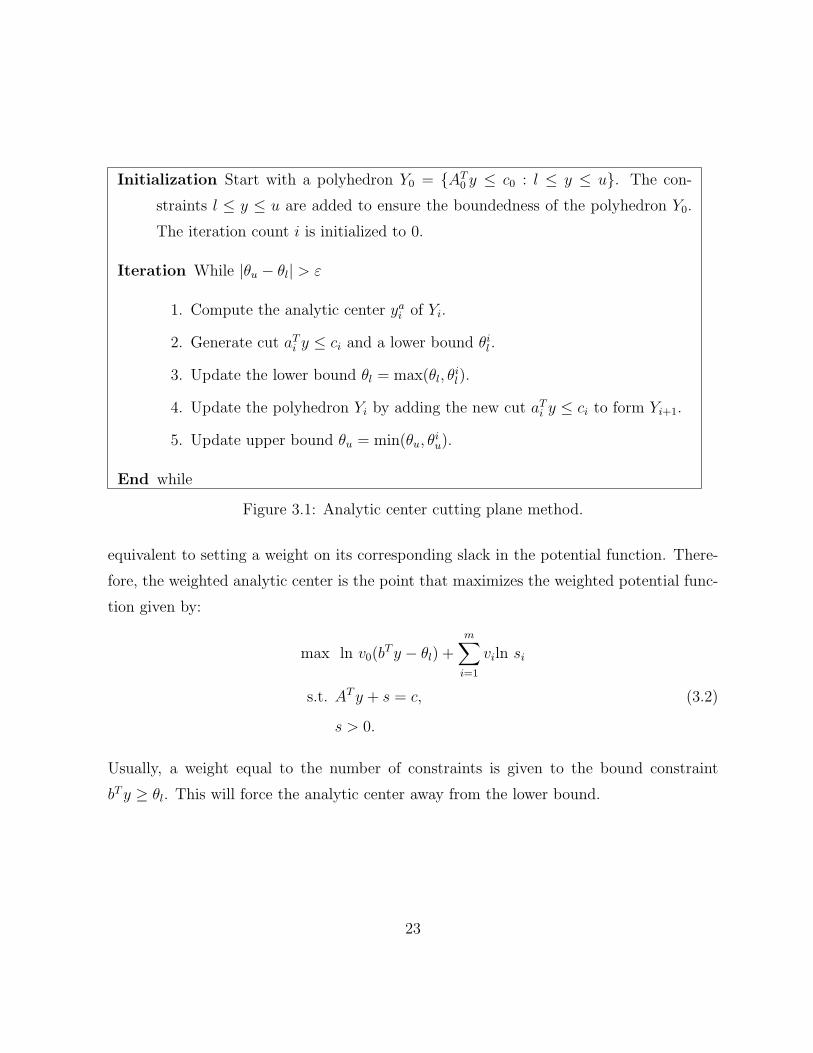
Initialization Start with a polyhedron Y0 = {AT0 y ≤ c0 : l ≤ y ≤ u}. The con-

straints l ≤ y ≤ u are added to ensure the boundedness of the polyhedron Y0.

The iteration count i is initialized to 0.

Iteration While |θu − θl| > ε

1. Compute the analytic center yai of Yi.

2. Generate cut aTi y ≤ ci and a lower bound θi

l .

3. Update the lower bound θl = max(θl, θil).

4. Update the polyhedron Yi by adding the new cut aTi y ≤ ci to form Yi+1.

5. Update upper bound θu = min(θu, θiu).

End while

Figure 3.1: Analytic center cutting plane method.

equivalent to setting a weight on its corresponding slack in the potential function. There-

fore, the weighted analytic center is the point that maximizes the weighted potential func-

tion given by:

max ln v0(bT y − θl) +

m∑i=1

viln si

s.t. AT y + s = c, (3.2)

s > 0.

Usually, a weight equal to the number of constraints is given to the bound constraint

bT y ≥ θl. This will force the analytic center away from the lower bound.

23

The first order optimality conditions for problem (3.2) are:

Sx = ν (3.3)

Ax = 0, x > 0 (3.4)

AT y + s = c, s > 0 (3.5)

where x = [x0, x]T , c = [−θl, c]T , s = [s0, s]

T , s0 = bT y − θl, A = [−b, A] and ν =

[m, 1, 1, . . . , 1]T . If a primal feasible solution x > 0 is available, then a primal Newton

method is used. If a dual feasible solution s > 0 is available, then a dual Newton method

is used. If both a primal and a dual feasible points are available, then a primal-dual New-

ton method is used. Details of these methods are provided in Ye (1997) and Elhedhli and

Goffin (2004).

3.2.1 Integer Analytic Centers

The analytic center presented in Section 3.2 assumes a continuous problem while the fea-

sible region of the Benders master problem is defined over discrete points only. In this

setting, the integer analytic center is defined as the closest discrete point to the continuous

analytic center. Consider a relaxed Benders master problem of the following form:

max {bT y : AT y ≤ c, y integer}.

To find the integer analytic center of the set Y = {AT y ≤ c, y integer}, we first start by

finding the continuous analytic center yac of the LP relaxation YLP = {AT y ≤ c}. To find

the closest integer point to yac, a minimum distance problem of the following form is solved

min ||y − yac||

s.t. Ay ≤ c, (3.6)

y integer.

Note that if the L1-norm is used to compute the distance ||y − yac|| then problem (3.6) is

a linear integer problem. This method was used in Atlason et al. (2004) in a simulation

24

based ACCPM. Results showed that solving problem (3.6) is computationally expensive

and it is advisable to use a heuristic to approximate the integer analytic center from the

continuous one. This is detailed in Section 3.4.1.

In the following section we present a cutting plane algorithm formed of two phases.

In the first phase, ACCPM is used to solve the LP relaxed problem. At each iteration, a

heuristic is used to approximate the integer analytic center which is used to generate cuts

that are valid to the original integer problem. In the second phase, Kelley’s cutting plane

method is used to solve the integer problem, warm started with the valid cuts generated

in phase I.

3.3 A Two-Phase ACCPM Algorithm

This section describes the two-phase ACCPM algorithm for solving mixed integer problems

taking the form (2.7)-(2.10). In the first phase of the algorithm, Benders decomposition is

used to solve the LP relaxation:

min cT x + dT y

s.t. A1y ≤ b1,

A2x + My ≥ b2,

y ≥ 0,

x ≥ 0.

The solution of the LP relaxed master problem, which may not necessarily be integer,

is used to solve the subproblem and generate a new constraint. Since the IP region is

contained in the LP region, then all the cuts that are valid to the LP problem are valid

to the IP problem. In addition to the cuts that are generated from non-integer points,

heuristics may be used to find integer points that are feasible to the IP master problem.

These integer points are used to solve the subproblem and generate new constraints that

25

are valid to the IP problem. Therefore by solving the LP relaxed problem, it is expected

that a good number of cuts that are valid to the IP problem would be generated. These

cuts are appended to the IP problem which is solved in phase II. Then by using Benders

decomposition to solve the IP problem, the appended valid cuts are expected to reduce the

number of iterations in which an integer master problem is solved.

ACCPM is used to solve the LP problem of phase I. The analytic center of the master

problem is used to generate cuts from the subproblem. Let yacLP be the continuous analytic

center of the polyhedron Y1 = {A1y ≤ b1}. The integer analytic center yacIP is defined as

the closest integer point to yacLP . The integer analytic center can be either found by solving

the minimum distance problem (3.6) or can be estimated using heuristics as detailed in

section 3.4.1. The IP analytic center is used to generate cuts from the subproblem. These

cuts are only valid to the IP master problem. We refer to LP central cuts as the feasibility

and optimality cuts generated from the LP analytic center whereas the IP central cuts are

the feasibility and optimality cuts generated from the IP analytic center. The two-phase

ACCPM algorithm is described below:

Phase-I:

Initialization Initialize θl and θu to the initial lower and upper bounds, and choose a

stopping parameter ε.

Iteration while |θu − θl| > ε

1. Compute the LP analytic center of the LP relaxed master problem

2. Use the LP analytic center to solve the subproblem and generate LP cuts

3. Append the LP cuts to the LP relaxed master problem and to the IP master

problem

4. Use the LP analytic center to compute the IP analytic center

26

5. Use the IP analytic center to solve the subproblem and generate IP cuts

6. Append the IP cuts to the IP master problem

7. Update upper and lower bounds

End while

Phase-II:

Initialization Initialize θl and θu to the initial lower and upper bounds, and choose a

stopping parameter ε. Append all the central cuts generated from Phase-I to the IP

master problem

Iteration while |θu − θl| > ε

1. Solve the IP master problem

2. Use the solution of the master problem to solve the subproblem and generate a

cut

3. Append the generated cut to the master problem

4. Update upper and lower bounds

End while

In the following section, the UMTS/W-CDMA network problem is solved using the two-

phase ACCPM. Furthermore, we discuss how the upper and lower bounds are obtained in

each phase.

3.4 Solving the UMTS/W-CDMA network planning

problem via the two-phase ACCPM

As detailed in section 2.3, the UMTS/W-CDMA network planning problem can be solved

iteratively through Benders decomposition where the master problem (2.27)-(2.32) and the

27

dual subproblem (2.25)-(2.26) are solved iteratively. As detailed in section 3.3, Phase I of

the algorithm solves the LP relaxation of the problem:

[OP-LP] : maxI∑i

riUizi −J∑j

cjyj − λI∑i

Uipi

s.t. xij − yj ≤ 0 ∀i,∀j,


Ukgkjpk + η]SIRmin ≥ (xij − 1)Mij ∀i,∀j,

zi −J∑j

xij ≤ 0 ∀i,

I∑i

Uizi ≥ πI∑i

Ui,

0 ≤ pi ≤ pmax ∀i,

0 ≤ zi ≤ 1, 0 ≤ yj ≤ 1, 0 ≤ xij ≤ 1 ∀i,∀j,

where the LP master problem is:

[MP-LP] : maxI∑i

riUizi −J∑j

cjyj − λθ

s.t. θ −I∑i

J∑j


I∑i

αhi +

I∑i

J∑j

(ηSIRmin −Mij)βhij ∀h ∈ HP , (3.7)

−I∑i

J∑j


I∑i

αhi +

I∑i

J∑j

(ηSIRmin −Mij)βhij ∀h ∈ HR, (3.8)

xij − yj ≤ 0 ∀i,∀j, (3.9)

zi −J∑j

xij ≤ 0 ∀i, (3.10)

I∑i

Uizi ≥ πI∑i

Ui, (3.11)

0 ≤ zi ≤ 1, 0 ≤ yj ≤ 1, 0 ≤ xij ≤ 1. (3.12)

28

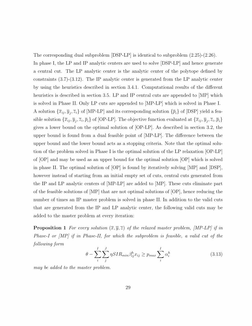
The corresponding dual subproblem [DSP-LP] is identical to subproblem (2.25)-(2.26).

In phase I, the LP and IP analytic centers are used to solve [DSP-LP] and hence generate

a central cut. The LP analytic center is the analytic center of the polytope defined by

constraints (3.7)-(3.12). The IP analytic center is generated from the LP analytic center

by using the heuristics described in section 3.4.1. Computational results of the different

heuristics is described in section 3.5. LP and IP central cuts are appended to [MP] which

is solved in Phase II. Only LP cuts are appended to [MP-LP] which is solved in Phase I.

A solution {xij, yj, zi} of [MP-LP] and its corresponding solution {pi} of [DSP] yield a fea-

sible solution {xij, yj, zi, pi} of [OP-LP]. The objective function evaluated at {xij, yj, zi, pi}gives a lower bound on the optimal solution of [OP-LP]. As described in section 3.2, the

upper bound is found from a dual feasible point of [MP-LP]. The difference between the

upper bound and the lower bound acts as a stopping criteria. Note that the optimal solu-

tion of the problem solved in Phase I is the optimal solution of the LP relaxation [OP-LP]

of [OP] and may be used as an upper bound for the optimal solution [OP] which is solved

in phase II. The optimal solution of [OP] is found by iteratively solving [MP] and [DSP],

however instead of starting from an initial empty set of cuts, central cuts generated from

the IP and LP analytic centers of [MP-LP] are added to [MP]. These cuts eliminate part

of the feasible solutions of [MP] that are not optimal solutions of [OP], hence reducing the

number of times an IP master problem is solved in phase II. In addition to the valid cuts

that are generated from the IP and LP analytic center, the following valid cuts may be

added to the master problem at every iteration:

Proposition 1 For every solution (x, y, z) of the relaxed master problem, [MP-LP] if in

Phase-I or [MP] if in Phase-II, for which the subproblem is feasible, a valid cut of the

following form

θ −I∑i

J∑j

ηSIRminβhijxij ≥ pmax

I∑i

αhi (3.13)

may be added to the master problem.

29

Proof: Consider an optimal solution (x∗, y∗, z∗, θ∗) of the full master problem, and suppose

that constraint (3.13) is violated, i.e.

θ∗ < pmax

I∑i

αhi +

I∑i

J∑j

ηSIRminβhijx

∗ij.

The optimal objective function value of the subproblem for fixed (x∗, y∗, z∗) is

θ = pmax

I∑i

αhi +

I∑i

J∑j

ηSIRminβhijx

∗ij.

Given an optimal solution (x∗, y∗, z∗) of the relaxed master problem and an optimal objec-

tive function value θ of the subproblem, then (x∗, y∗, z∗, θ) is a feasible solution of the full

master problem and has an objective function value Z [FMP ] =∑I

i riUiz∗i −

∑Jj cjy

∗j − λθ.

Since the full master problem is a maximization problem, this value is then a lower bound

on its optimal objective function value. The objective function evaluated at (x∗, y∗, z∗, θ∗)

is equal to

Z∗[FMP ] =

I∑i

riUiz∗i −

J∑j

cjy∗j − λθ∗.

Since

θ∗ < pmax

I∑i

αhi +

I∑i

J∑j

ηSIRminβhijx

∗ij = θ.

then

Z∗[FMP ] < Z [FMP ]

and (x∗, y∗, z∗, θ∗) is not an optimal solution. Furthermore, in order to have an optimal

solution (x∗, y∗, z∗, θ∗), we should have

Z∗[FMP ] ≥ Z [FMP ]

and therefore

θ∗ ≥ pmax

I∑i

αhi +

I∑i

J∑j

ηSIRminβhijx

∗ij.

�

30

Proposition 2 For every solution (x, y, z) of the relaxed master problem, [MP-LP] if in

Phase-I or [MP] if in Phase-II, for which the subproblem is infeasible, a valid cut of the

following form

−I∑i

J∑j

ηSIRminβhijxij ≥ pmax

I∑i

αhi (3.14)

may be added to the master problem.

Proof: Consider a solution (x, y, z) of the relaxed master problem for which the subprob-

lem is infeasible, then the feasibility cut

−I∑i

J∑j


I∑i

αhi +

I∑i

J∑j

(ηSIRmin −Mij)βhij

is added to the master problem, where (αh, βh) are the components of the extreme ray gen-

erated by solving the alternative subproblem. Consider an optimal solution (x∗, y∗, z∗, θ∗)

of the full master problem that violates constraint (3.14), that is,

pmax

I∑i

αhi +

I∑i

J∑j

ηSIRminβhijx

∗ij > 0. (3.15)

Furthermore, since (αhi , β

hij) are the components of the extreme ray, then they satisfy

αhi +

J∑j

βhij(SFgij − (Ui − 1)gijSIRmin)− SIRmin

∑k 6=i

∑j

Ukgkjβhkj ≤ 0. (3.16)

Having inequalities (3.15) and (3.16), implies that the auxiliary subproblem [ASP] with x =

x∗ has a feasible solution (αhi , β

hij) and hence [DSP] is unbounded. Therefore, (x∗, y∗, z∗, θ∗)

is not a feasible solution of the full master problem. �

3.4.1 Heuristics for finding the IP analytic center

As described in section 3.2.1, solving problem (3.6) is computationally expensive and there-

fore heuristics are used to find feasible solutions. In this section we describe five heuristics

31

that can be used to find integer solutions. Heuristic 1 is a generic heuristic that can be used

to find feasible solutions of any MIP problem while the other four heuristics are specific to

the UMTS/W-CDMA network planning problem.

Heuristic 1 - Central Rounding

Many heuristics address the problem of finding a feasible solution of the generic MIP

problem

min bT y

s.t. AT y ≤ c, (3.17)

yj integer ∀j ∈ G, (3.18)

yj ≥ 0 ∀j ∈ C. (3.19)

The feasibility pump, was recently introduced by Fischetti et al. (2005). This heuristic

iteratively solves the LP relaxation of the MIP problem to generate a point y∗ which is

rounded to the nearest integer point y. The first point satisfies the LP constraints while

the other satisfies the integrality constraints. Hopefully, the two points will converge to the

same point within a finite number of iterations. Tests revealed that this algorithm suffers

from stalling where the same points are generated repeatedly. Random perturbation that

randomly shifts the values of y up and down is effective in solving the stalling issue. The

feasibility pump was proved to be successful for finding feasible solutions for 0-1 MIP

problems, however it fails to solve problems with general integer variables. A rather more

complicated extension of the feasibility pump is introduced in Bertacco et al. (2007). This

extension improves the original feasibility pump so as to solve MIP problems with general

integer variables. In addition to its complicated implementation, this method does not

present any guarantees in terms of the quality of the feasible solution. This is mainly due

to the fact that the objective function of the MIP is not used to find y∗ and y.

32

yfp

yac

Figure 3.2: Rounding to the nearest integer. yac: Analytic Center, yfp: Feasibility Pump solution,

→: Nearest integer point.

Central rounding is a new heuristic that takes advantage of analytic centers to generate

feasible solutions of MIP problems. Compared to the feasibility pump, the efficiency of this

algorithm stems from the fact that the analytic center lies near the center of the feasible

region (Figure 3.2), so rounding to the nearest integer will most likely result in a feasible

integer point. Considering problem (3.17)-(3.19), central rounding proceeds as follows:

The continuous analytic center yac of the localization set

F =

bT y ≤ zu

AT y ≤ c

y ≥ 0

is calculated. An integer point yI is found by rounding yac to the nearest integer point. If

yI is a feasible point, then the algorithm stops. On the other hand, if yI is not feasible then

the weight of the violated constraint is increased and the analytic center is recomputed. As

detailed in section 3.2, the new weight will force the analytic center away from the violated

33

constraint and a new integer point is found by rounding to the nearest integer. This process

is repeated until a feasible integer point is found. Unfortunately, the process of pushing the

integer points towards feasibility is very slow and the weights might significantly increase

so as to create computational problems. Having a weight on a constraint is identical

to replicating the constraint. Therefore instead of incrementing the weight of the violated

constraint, this constraint is replicated and appended to the set of constraints. Additionally

in order to accelerate the process of finding a feasible integer solution, the right hand side

of the added constraint is modified as follows:

Let yac be the continuous analytic center with yI being the corresponding nearest integer

point. Suppose that yI is infeasible to constraint A1y ≤ c1. Knowing that replicating

constraint A1y ≤ c1 will push the new analytic center y away from it such that A1y ≤A1y

ac ≤ c1 the right hand side of the replicated constraint is modified such that A1y ≤A1y

ac. Note that yac is still a primal feasible point and therefore a new analytic center

for the updated polyhedron can be computed efficiently. Note that in contrast to the

feasibility pump, this algorithm does not suffer from stalling since at each iteration either

a feasible integer solution is found or a cut that eliminates the current LP solution is added.

Furthermore, the quality of the solution is insured by the bound zu in the definition of the

localization set F . If the resulting feasible integer solution yI does not satisfy the required

quality, then the bound is set to zu = bT yI and the heuristic is rerun. This ensures a better

quality solution in the next run. In the very first run zu is set to +∞.

In the two-phase ACCPM algorithm, central rounding is used to find a feasible integer

solution of problem (3.6).

Heuristic 2

Similar to the central rounding heuristic, an integer point is found by rounding the LP

analytic center to the nearest integer point. Moreover, whether the resulting integer point

is feasible or not, a valid cut is generated from the subproblem. To show this, we consider

the following

34

Lemma 1 Every cut generated from the subproblem (2.16) is a valid cut.

Proof: Consider a solution y not necessarily feasible to the full master problem (2.12)-

(2.15). Using y, let λ be the optimal solution of the subproblem (2.16) and a cut

(b2 −My)λ ≤ θ (3.20)

is generated. Consider an optimal solution (y∗, θ∗) of the full master problem that violates

constraint (3.20), i.e.

(b2 −My∗)λ = θ > θ∗.

Note that (y∗, θ) is a feasible solution of the full master problem. The objective function

of the full master problem evaluated at (y∗, θ) is equal to

Z [FMP ] = dT y∗ + θ.

The objective function of the full master problem evaluated at (y∗, θ∗) is equal to

Z∗[FMP ] = dT y∗ + θ∗.

Since

θ > θ∗,

then

Z [FMP ] > Z∗[FMP ]

and (y∗, θ∗) is not an optimal solution. �

Heuristic 3

In this heuristic, the values of xij are rounded to the nearest integer. Therefore, if xij < 0.5

then set xij = 0 otherwise set xij = 1. Furthermore, if∑

i xij ≥ 1 then set yj = 1 otherwise

set yj = 0. Additionally, if∑

j xij ≥ 1 then set zi = 1 otherwise set zi = 0.

35

Heuristic 4

Initialize yj = 0, ∀j and zi = 0, ∀i. For each demand point i, find a base station j such

that xij = maxj

xij and then set xij = 1, xik = 0, ∀k 6= j, yj = 1 and finally zi = 1.

Heuristic 5

Initialize yj = 0, ∀j and zi = 0, ∀i. Additionally, let LPmax = max xij, LPmin = min xij. If

xij ≥ (LPmax−LPmin)/2 then set xij = 1, zi = 1, and yj = 1, otherwise set xij = 0. Note,

that the resulting solution might violate constraint (2.31). In this case, find a demand

point i such that zi = 0, find a base station j such that xij = maxj

xij then set xij = 1,

zi = 1 and yj = 1. This process is repeated until constraint (2.31) is satisfied.

3.5 Computational Results

The classical Benders decomposition and the two-phase ACCPM were implemented in C

and run on a Sunblade 2500 workstation with two 1.6 GHz processors and 2 Gb of RAM.

The master problems and the subproblems were solved using cplex 10.1. Computational

testing was done on a set of instances proposed by Amaldi et al. (2002). Potential base

station and user locations were randomly selected from these instances. Propagation gains

gij are calculated using Hata (1980) propagation model. The gain in dB is calculated as

follows:

Aij = 69.55 + 26.16 log(f)− 13.82 log(Hj)

− [(1.1 log(f)− 0.7)Hi − (1.56 log(f)− 0.8)]

+ [4.99− 6.55 log(Hj)] log(dij)

where f is the center frequency measured in Mhz, Hi is the height of the transmitter at

location i and Hj is the height of the base station at location j. Hi and Hj are measured

36

Data Value Description

SIRmin 0.01 Minimum SIR

f 2000 Operating frequency

Hj 10 m Height of base station antenna

Hi 1 m Height of mobile device antenna

SF 128 Spreading Factor

η 6.3e-14 Receiver thermal noise

pmax 0.15 Maximum power

r 145 Revenue from each serviced user

c 42 Base station cost

λ 0.42 Power cost

Table 3.1: Data for the test cases

in meters. Aij is converted to propagation gain as follows

gij = 10−0.1Aij .

Parameters used for the test problems are shown in Table 3.1. We evaluate the effect

of generating feasible cuts from the analytic center of the master problem through the

two-phase ACCPM algorithm. The performance of the two-phase ACCPM algorithm is

compared to the classical Benders decomposition algorithm. Results for 14 test cases

solved using the classical Benders decomposition are shown in Table 3.2. For each test

case, we ran 10 randomly generated problems and took the average. The first column

of the table indicates the test case number. The second and third columns indicate the

number of demand points (#DP) and the number of candidate base station locations

(#BS) respectively. Column (4) indicates the number of iterations (Iter) and consequently

the number of times the integer Benders master problem is solved. Finally, column (5)

indicates the total CPU time in seconds spent on solving each test case.

37

Test Case #DP #BS IterIP CPU (s)

(1) (2) (3) (4) (5)

1 8 2 28.1 1.7

2 9 2 39.2 2.9

3 10 2 43.4 5.0

4 5 3 33.1 2.4

5 6 3 55.9 7.1

6 7 3 95.5 25.4

7 8 3 131 59.1

8 9 3 203.4 206.6

9 10 3 225.7 637.3

10 5 4 65 12.5

11 6 4 126.2 49.5

12 7 4 221 212.8

13 8 4 433.6 2031.5

14 9 4 780 17722.3

Table 3.2: Computational Results - Classical Benders Decomposition

Phase-I Phase-II

Test Case #DP #BS IterLP CPU (s) IterIP CPU (s) CPU (s)

(1) (2) (3) (4) (5) (6) (7) (8)

1 8 2 14.2 1.6 20.9 1.2 2.8

2 9 2 15.4 2 30.9 2.3 4.3

3 10 2 16.4 2.6 32 3.7 6.3

4 5 3 15.9 1.2 23.8 1.8 3

5 6 3 17.9 1.9 43.9 5.6 7.5

6 7 3 22.4 4.0 73.5 19.5 23.5

7 8 3 24.2 4.9 111.7 50.6 55.5

8 9 3 25.9 7 183.4 186.3 193.3

9 10 3 30.1 11.1 201.6 569.3 580.4

10 5 4 21.6 2.6 48.7 9.4 12.0

11 6 4 25.3 5.3 106.9 42.1 47.4

12 7 4 27.4 7.3 195.1 187.9 195.2

13 8 4 32.1 13.6 399.3 1871.1 1884.7

14 9 4 35.7 18 686.6 15598.3 15616.3

Table 3.3: Computational Results - Two-phase ACCPM Algorithm

38

The same 14 test cases are solved using the two-phase ACCPM algorithm and the re-

sults are shown in Table 3.3. Column (4) of the table indicates the number of iterations

(IterLP) required to solve the LP relaxed problem (also indicates the number of valid cuts

that are generated and added to the problem solved in Phase II). Column (5) indicates

the CPU time required to solve the LP relaxed problem in Phase I. Column (6) indicates

the number of iterations (IterIP) required to solve the problem in Phase II (also indicates

the number of times the integer Master problem is solved). Column (7) indicates the CPU

time required to solve the problem in Phase II. Finally Column (8) shows the total CPU

time required by the two-phase ACCPM algorithm; that is the time spent on Phase I in

addition to the time spent on Phase II.

We observe that the two-phase ACCPM algorithm becomes more efficient as the com-

plexity of the problem increases. We notice that adding valid cuts from Phase-I always

reduces the number of iterations and consequently the computational time of solving the

integer problem in Phase-II. However, we notice that for relatively very small instances

(test cases 1 through 5), even though the computational time required to solve the integer

problem is decreased, the classical Benders decomposition achieves a better overall com-

putational time. This is due to the overhead computational time required to generate the

valid cuts using ACCPM in Phase-I, and indicates that a more efficient implementation

of ACCPM will certainly enhance the two-phase ACCPM algorithm. For larger instances

(test cases 6 through 14), we observe that the two-phase ACCPM algorithm takes less

computational time than the classical Benders decomposition. Moreover, for test case 6,

the computational time is reduced by 10%. On the other extreme, the computational time

for test case 14 is reduced by 12%.

In an attempt to generate more cuts from Phase-I, we evaluate the performance of the

two-phase ACCPM algorithm with the weight of the bound constraint set to 1. Recall

from Section 3.2 that the weight of the bound constraint is set to be equal to the number

39

Phase-I Phase-II


(1) (2) (3) (4) (5) (6) (7) (8)

1 8 2 25.9 2.5 13.4 0.74 3.2

2 9 2 28.7 3.6 22.8 1.7 5.3

3 10 2 30.5 4.8 26 3 7.8

4 5 3 26.0 1.9 18.9 1.4 3.3

5 6 3 27.8 2.9 39 5 7.9

6 7 3 32.6 4.6 73.3 19.5 24.1

7 8 3 35.0 6.8 104.4 47.1 53.9

8 9 3 39.6 9.9 172 175.1 185.0

9 10 3 40.6 13.3 192.7 544.5 557.8

10 5 4 31.9 3.7 43.6 8.4 12.1

11 6 4 38.1 6.8 102.1 40 46.8

12 7 4 41.4 10.2 188.8 181.7 191.9

13 8 4 45.6 15.3 394.3 1848.3 1863.6

14 9 4 51.3 23.5 629.2 14296.2 14319.7

Table 3.4: Computational Results - Two-phase ACCPM Algo. - Weight of bound constraint

set to 1

of constraints. This reduces the number of iterations required by ACCPM to solve the LP

problem. Since at each ACCPM iteration a valid cut is generated, reducing the number

of iterations reduces the number of generated cuts. The 14 test cases are solved using

the two-phase algorithm with the weight on the objective function set to 1. The results

are shown in Table 3.5. We observe that the number of iterations of ACCPM in Phase-I

and therefore the number of generated cuts is increased by approximately 50%. This is

reflected in an increase in the computational time spent on solving Phase-I. However, this

increase is compensated by a reduction in computational time spent on solving Phase-II.

We observe that the additional cuts improve the computational performance of the two-

phase algorithm.

To evaluate the effect of the central cuts, we compare the two-phase algorithm where

valid cuts are generated from the analytic center of the master problem to a two-phase

algorithm where valid cuts are generated from the extreme point (optimal solution) of

the master problem (i.e., we compare the algorithm when in the first phase the master

problem is solved using the analytic center cutting plane method and when it is solved using

Kelley’s cutting plane method). Results for the 14 test cases solved using the two-phase

40

Phase-I Phase-II


(1) (2) (3) (4) (5) (6) (7) (8)

1 8 2 9.3 0.0 22.6 1.3 1.3

2 9 2 11.0 0.1 31.8 2.4 2.5

3 10 2 11.3 0.1 35.8 4.2 4.3

4 5 3 12.0 0.0 24.3 1.8 1.8

5 6 3 15.2 0.1 45.5 5.8 5.9

6 7 3 18.3 0.1 76.0 20.2 20.3

7 8 3 19.0 0.1 115.6 52.2 52.3

8 9 3 23.3 0.2 184.4 187.4 187.6

9 10 3 25.0 0.2 207.3 585.4 585.6

10 5 4 19.3 0.1 51.3 9.86 9.9

11 6 4 25.0 0.1 109.9 43.2 43.3

12 7 4 26.6 0.2 200.0 192.6 192.8

13 8 4 31.4 0.3 408.8 1915.4 1915.7

14 9 4 36.0 0.4 706.7 16056.7 16057.1

Table 3.5: Computational Results - Two-phase Algorithm - Kelley Based

Kelley’s cutting plane algorithm are shown in Table 3.5. We observe that the two-phase

Kelley’s based algorithm achieves better performance compared to the classical Benders

algorithm. Compared to the ACCPM based algorithm, we observe that Kelley’s cutting

plane algorithm performs less iterations in Phase-I. This is also reflected in a significantly

less computational time spent on solving Phase-I. This justifies our previous conclusion

that a more efficient implementation of ACCPM will improve the overall performance of

the two-phase algorithm. In Phase-II, ACCPM based algorithm consumes less iterations

and consequently less time. Overall, Kelley’s based algorithm achieves better performance

for the relatively small instances (test cases 1 through 5) however for larger instances where

the classical Benders decomposition suffers, we observe that the ACCPM based algorithm

achieves better computational time compared to the Kelley’s based algorithm.

Finally, we evaluate the effect of the rounding heuristics on the two-phase ACCPM

algorithm. Since setting the weight on the bound constraint to 1 was shown to be beneficial,

we use this same weight for the remaining tests. Results for the 14 test cases solved using

the two-phase ACCPM with rounding Heuristic 1 are shown in Table 3.5. Eventhough

Heuristic 1 (Central Rounding) consumes a significant time to find feasible integer solutions,

41

Phase-I Phase-II

Test Case #DP #BS IterLP CPU (s) CPUH IterIP CPU (s) CPU (s)

(1) (2) (3) (4) (5) (6) (7) (8) (9)

1 8 2 25.9 2.5 6.0 9.5 0.5 9.0

2 9 2 28.7 3.6 11.7 17.7 1.3 16.6

3 10 2 30.5 4.8 1.9 15.1 1.9 8.5

4 5 3 26.0 1.9 5.9 13.3 1.0 8.8

5 6 3 27.8 2.9 10.1 29.5 3.8 16.8

6 7 3 32.6 4.6 16.9 51.9 13.8 35.3

7 8 3 35.0 6.8 28.7 77.5 41.3 76.7

8 9 3 39.6 9.9 44.3 138.3 158.5 212.7

9 10 3 40.6 13.3 68.5 154.5 436.3 518.2

10 5 4 31.9 3.7 18.6 35.1 6.8 29.1

11 6 4 38.1 6.8 35.8 77.5 30.4 72.9

12 7 4 41.4 10.2 61.1 173.6 167.2 238.4

13 8 4 45.6 15.3 101.0 371.3 1739.6 1855.9

14 9 4 51.3 23.5 108.5 602.1 13680.3 13812.3

Table 3.6: Computational Results - Two-phase ACCPM Algo. - Rounding Heuristic 1

generating cuts from integer solutions reduce the number of iterations in Phase-II of the

algorithm. The computational overhead of finding feasible integer solutions makes the use

of Heuristic-1 only beneficial in large instances where the computational time of Heuristic-1

is less significant and a better performance of the two-phase ACCPM algorithm is achieved.

Heuristic-1 is computationally expensive since it is a generic heuristic that can be applied

to any mixed integer problem. The remaining 4 heuristics are specific heuristics that

apply to the UMTS/W-CDMA network planning problem. Results for the 14 test cases

solved using the two-phase ACCPM algorithm with Heuristic-2, Heuristic-3, Heuristic-4

and Heuristic-5 are shown in Tables 3.7, 3.8, 3.9 and 3.10 respectively. The computational

time of these heuristics is negligible so it is not explicitly shown in the tables. Results show

that all these heuristics improve the computational performance of the two-phase ACCPM

algorithm. Additionally, Heuristic-2 and Heuristic-3 achieve identical results since the cuts

generated from the subproblem depend only on the xij variables, and these two heuristics

behave similarly in terms of the xij variables. Heuristic-4 and Heuristic-5 achieve better

results than Heuristic-2 and Heuristic-3. Finally, by comparing the computational results

of Phase-II, we notice that Heuristic-1 achieves the best results compared to the other 4

heuristics. However due to the computational burden of Heuristic-1, only large instances

42

achieve a better overall performance. A summary of the results is presented in Figures 3.3

and 3.4.

Phase-I Phase-II


(1) (2) (3) (4) (5) (6) (7) (8)

1 8 2 25.9 2.5 9.7 0.5 3.0

2 9 2 28.7 3.6 18.5 1.4 5.0

3 10 2 30.5 4.8 15.5 1.9 6.7

4 5 3 26.0 1.9 15.2 1.1 3.0

5 6 3 27.8 2.9 31.1 4.1 7.0

6 7 3 32.6 4.6 64.2 17.4 22.0

7 8 3 35.0 6.8 90.7 41.7 48.5

8 9 3 39.6 9.9 153.9 160.2 170.1

9 10 3 40.6 13.3 170.3 482.1 495.4

10 5 4 31.9 3.7 41.4 7.9 11.6

11 6 4 38.1 6.8 96.5 37.6 44.4

12 7 4 41.4 10.2 185.0 177.8 188.0

13 8 4 45.6 15.3 390.5 1827.6 1842.9

14 9 4 51.3 23.5 629.3 14291.9 14315.4


Phase-I Phase-II


(1) (2) (3) (4) (5) (6) (7) (8)

1 8 2 25.9 2.5 9.7 0.5 3.0

2 9 2 28.7 3.6 18.5 1.4 5.0

3 10 2 30.5 4.8 15.5 1.9 6.7

4 5 3 26.0 1.9 15.2 1.1 3.0

5 6 3 27.8 2.9 31.1 4.1 7.0

6 7 3 32.6 4.6 64.2 17.4 22.0

7 8 3 35.0 6.8 90.7 41.7 48.5

8 9 3 39.6 9.9 153.9 160.2 170.1

9 10 3 40.6 13.3 170.3 482.1 495.4

10 5 4 31.9 3.7 41.4 7.9 11.6

11 6 4 38.1 6.8 96.5 37.6 44.4

12 7 4 41.4 10.2 185.0 177.8 188.0

13 8 4 45.6 15.3 390.5 1827.6 1842.9

14 9 4 51.3 23.5 629.3 14291.9 14315.4


43

Phase-I Phase-II


(1) (2) (3) (4) (5) (6) (7) (8)

1 8 2 25.9 2.5 9.3 0.5 3.0

2 9 2 28.7 3.6 15.3 1.2 4.8

3 10 2 30.5 4.8 15.3 1.8 6.6

4 5 3 26.0 1.9 15.1 1.1 3.0

5 6 3 27.8 2.9 30.7 4.0 6.9

6 7 3 32.6 4.6 63.1 17.1 21.7

7 8 3 35.0 6.8 87.1 41.1 47.9

8 9 3 39.6 9.9 149.1 152.1 162.0

9 10 3 40.6 13.3 161.3 456.1 469.4

10 5 4 31.9 3.7 41.1 7.8 11.5

11 6 4 38.1 6.8 96.2 37.6 44.4

12 7 4 41.4 10.2 184.7 177.4 187.6

13 8 4 45.6 15.3 382.5 1791.1 1806.4

14 9 4 51.3 23.5 617.5 14031.9 14055.4


Phase-I Phase-II


(1) (2) (3) (4) (5) (6) (7) (8)

1 8 2 25.9 2.5 9.5 0.5 3.0

2 9 2 28.7 3.6 17.3 1.3 4.9

3 10 2 30.5 4.8 15.8 1.9 6.7

4 5 3 26.0 1.9 15.5 1.2 3.1

5 6 3 27.8 2.9 31.5 4.1 7.0

6 7 3 32.6 4.6 63.9 17.3 21.9

7 8 3 35.0 6.8 87.1 40.2 47.0

8 9 3 39.6 9.9 150.7 154.7 164.6

9 10 3 40.6 13.3 161.3 456.9 470.2

10 5 4 31.9 3.7 42.3 8.2 11.9

11 6 4 38.1 6.8 97.9 38.2 45.0

12 7 4 41.4 10.2 184.1 176.9 187.1

13 8 4 45.6 15.3 384.7 1801.1 1816.4

14 9 4 51.3 23.5 620.2 14091.2 14114.7


44

0

150

300

450

600

750

900

0 1 2 3 4 5 6 7 8 9 10 11 12 13 14

Test Case

Num

ber o

f IP

Iter

atio

ns

Classical Bender Decomp. 2-Phase ACCPM 2-Phase ACCPM - Weights set to 12-Phase - Kelly Based 2-Phase ACCPM - Rounding Heuristic 1 2-Phase ACCPM - Rounding Heuristic 22-Phase ACCPM - Rounding Heuristic 3 2-Phase ACCPM - Rounding Heuristic 4 2-Phase ACCPM - Rounding Heuristic 5

Figure 3.3: Number of times the IP master problem is solved.

45

Classical Bender Decomp. 2-Phase ACCPM 2-Phase ACCPM - Weights set to 12-Phase - Kelly Based 2-Phase ACCPM - Rounding Heuristic 1 2-Phase ACCPM - Rounding Heuristic 22-Phase ACCPM - Rounding Heuristic 3 2-Phase ACCPM - Rounding Heuristic 4 2-Phase ACCPM - Rounding Heuristic 5

14000

16000

18000

0

200

400

600

800

1000

1200

1400

1600

1800

2000

0 1 2 3 4 5 6 7 8 9 10 11 12 13 14Test Case

Tim

e (s

ec.)

Figure 3.4: Total CPU time consumed by each algorithm.

46

In this chapter, the analytic center cutting plane method was used to generate valid

cuts. The computational results show that these valid cuts reduce the number of iterations

required to solve the MIP problem. In the following chapter we introduce a new decomposi-

tion approach that aims at reducing the complexity of the master problem by reducing the

number of integer variables in it. Therefore rather than having a master problem defined

over the full set of integer variables, the new decomposition approach formulates a master

problem defined over a subset of the integer variables while the remaining integer variables

are defined in the subproblem. This reduces the complexity of the master problem and

aims at eliminating the bottleneck of solving a hard MIP problem at every iteration.

47

Chapter 4

Nested and Combinatorial Benders

Decomposition Algorithms

Several techniques have been adopted to accelerate Benders decomposition. A new method

that utilizes the analytic center cutting plane method to generate cuts was introduced in

Chapter 3. Most research emphasizes accelerating Benders decomposition by reducing the

number of iterations, therefore reducing the number of times the master problem is solved

(see Chapter 3 for details). This chapter introduces a novel decomposition algorithm for

solving binary integer problems. Rather than reducing the number of iterations, the new

decomposition algorithm, Combinatorial Benders Decomposition, reduces the complexity

of the integer master problem by reducing the number of integer variables in it. The

resulting problem is formed by an integer master problem and an integer subproblem. The

subproblem is then decomposed using the classical Benders decomposition leading to a

nested Benders Decomposition. In the following section we present a general description of

the combinatorial Benders decomposition. Then a detailed description of nested Benders

decomposition applied to the UMTS/W-CDMA network planning problem follows.

48

4.1 Combinatorial Benders Decomposition Algorithm

Combinatorial Benders decomposition is applicable to MIP problems with the following

structure:

[P]: min cT x + dT y

s.t. Ax + My ≥ b,

xi ∈ {0, 1},

yj ∈ {0, 1} ∀j ∈ B,

yj integer ∀j ∈ G,

yj ≥ 0 ∀j ∈ C,

where x is a vector of binary variables and y is a vector of continuous, general-integer and

binary variables. The case where d = 0 is considered in Codato and Fischetti (2006). In

this work, we consider a general case where d 6= 0. In contrast to classical Benders decom-

position where the subproblems are linear programs, combinatorial Benders decomposition

leaves some of the integer variables for the subproblem, leading to a MIP subproblem. For

fixed x variables, [P ] may be rewritten as:

[MP]: min cT x + θ(x)

s.t. xi ∈ {0, 1},

where

[SP]: θ(x) = min dT y

s.t. My ≥ b− Ax,

yj ∈ {0, 1} ∀j ∈ B,

yj integer ∀j ∈ G,

yj ≥ 0 ∀j ∈ C.

49

For each xh optimal to [MP], there exists a single value θh = dT yh optimal to [SP]. Fur-

thermore, (xh, yh) is a feasible solution to [P]. Thus, the optimal solution of [P] is the best

objective function value of [MP] evaluated at all possible (xh, yh). If xh is infeasible for

[SP], then xh is infeasible for [P], thus at least one variable of xh should be changed in

order to make [SP] feasible. This is formulated as a feasibility cut of the form∑i:xh

i =0

xi +∑

i:xhi =1

(1− xi) ≥ 1

and appended to [MP ]. Otherwise, if there exists an optimal solution θh = dT yh of [SP]

when x is fixed to xh, a binary Benders cut of the form

Mh∑

i:xhi =0

xi + Mh∑

i:xhi =1

(1− xi) + θ ≥ θh (4.1)

is generated and appended to [MP ]. Mh is a large enough number that would make

constraint (4.1) only active for the corresponding xh. Hence, the master problem is:

[MP]: min cT x + θ

s.t. Mh∑

i:xhi =0

xhi + Mh

∑i:xh

i =1

(1− xhi ) + θ ≥ θh ∀h ∈ HP , (4.2)

∑i:xh

i =0

x~i +

∑i:xh

i =1

(1− x~i ) ≥ 1 ∀~ ∈ HR, (4.3)

xi ∈ {0, 1}, θ is free

where HP and HR are the sets of feasible and infeasible solutions to [SP]. If HP and HR

enclose all solutions that are feasible and infeasible to P , then [MP] is equivalent to [P].

Otherwise, [MP(HP , HR)] is a relaxation of [P] and the objective function value of [MP] is

a lower bound to the objective function value of [P]. Note that we assumed [MP] is always

feasible. If solving [MP] to optimality is infeasible then [P] is also infeasible. Similar to

the classical Benders decomposition algorithm, the upper and lower bounds are used as a

50

stopping criteria for the cutting plane algorithm. A description follows:

1. Start with UB = ∞ ; LB =−∞. h is the iterations count, h=1.

While LB 6= UB

2. Solve [MP] and get solution x, and a lower bound LBh.

3. Set LB = LBh.

4. Solve [SP]

4.1 If [SP] is infeasible

4.1.1 add feasibility cut of type (4.3)

4.2 If [SP] is feasible

4.2.1 Solve [SP] and get solution y, get UBh = cT x + bT yj

4.2.2 add optimality cut of type (4.2)

4.2.3 Update upper bound UB = min(UB,UBh)

End while

Since x ∈ {0, 1}, there exists a finite number of constraints of the form (4.2) and (4.3) that

may be appended to [MP]. Furthermore, none of the infeasible x variables may be generated

more than once from [MP] since each infeasible x is eliminated by adding a constraint of

type (4.3). If x is a feasible solution, then if x is generated twice, the algorithm terminates

with an optimal solution x (UB=LB). As none of the x’s are generated more than once,

the combinatorial Benders decomposition will converge in a finite number of iterations.

4.1.1 Ensuring a bounded [MP] formulation

The master problem [MP] defined by (4.2)-(4.3) is bounded only if all possible combinations

of the x variables are defined by the sets HP and HR. Since θ is a free variable, if there

exists a feasible solution xk where k /∈ {HP ∪ HR} then [MP] is unbounded. Therefore,

to ensure that [MP] is bounded at every iteration, the [MP] formulation should include

51

a lower bound on θ(x). Since by construction [SP] is always bounded or otherwise [P]

is unbounded, there always exists a lower bound LB([SP ]) = minx

[SP (x)], where x is a

feasible solution of [MP]. Therefore a constraint of the form

θ ≥ LB([SP ]) (4.4)

is added to the formulation of [MP] to ensure a bounded master problem. Alternatively if

LB([SP ]) is not known or cannot be easily found, a constraint of the form

θ ≥ min(θh)− ε ∀ h ∈ H (4.5)

may be added to [MP] to ensure boundedness, where ε is a positive number. In fact,

at each iteration the optimal solution of [MP] is either (xk, θk) with k = h ∈ HP , thus

θk = θh otherwise k /∈ H and θk is less than all θh generated so far. Note that in the case

where (4.5) is used instead of (4.4), if in an optimal solution constraint (4.5) is binding,

then the objective function cT xk + θk is no longer a lower bound on the optimal objective

function value of [P]. Alternatively, if (4.5) is not binding, therefore (4.5) has no effect on

the [MP] formulations presented in (4.2)-(4.3) hence cT xk + θk is a lower bound on the

optimal objective function value of [P]. We note that for the very first iteration, we may

add any lower bound on the value of θ. This will not affect the solution of [MP] since

none of the equations (4.2)-(4.3) is added and therefore would not affect the choice the x

variables. Afterwards, the lower bound on θ is updated as described.

4.1.2 Avoiding Total Enumeration

In the case where d 6= 0 and if constraint (4.5) is used instead of (4.4), the algorithm will

enumerate all possible combinations of the x variables before converging to an optimal

solution. In fact, if there exists a combination xk not visited (i.e. k /∈ {HP ∪HR}), then

there exists an optimal solution (xk, θk) of [MP] where none of the constraints of type (4.2)

is binding. To avoid a total enumeration case, it is advisable to exploit the structure of

[SP] thus using a heuristic to generate multiple cuts of type (4.2)-(4.3) at each iteration.

52

This may be implemented in the sense that if a solution xk is generated and if xp is known

to be worse than xk then xP cannot be part of an optimal solution. Hence, a constraint of

the form (4.3) may be generated to eliminate xp. In Section 4.3, a heuristic is implemented

to generate multiple cuts when solving the UMTS/W-CDMA network planning problem.

In the case where a similar heuristic cannot be implemented, it is advisable to apply the

discussed decomposition approach when the number of x variables is relatively small.

In the following section the combinatorial Benders decomposition is used along with the

classical Benders decomposition to form a nested Benders decomposition algorithm. This

algorithm is then used to solve the UMTS/W-CDMA network planning problem.

4.2 Nested Benders Decomposition

For large instances of the problem formulated in Section 2.4, large number of cuts may be

appended to the master problem before reaching an optimal solution. This increases the

computational time required to solve the mixed integer master problem. Motivated by the

fact that the number of base stations (yj variables) is relatively smaller than the number

of demand points (xij variables), fixing yj variables will significantly reduce the compu-

tational requirements of finding the xij variables. The same motivation was exploited

by Kalvenes et al. (2006) through priority branching over the base station locations in a

branch and bound algorithm. However for large instances, the branch and bound tree will

unreasonably grow to huge size. Fixing some binary variables through a Benders decom-

position is explored next.

For fixed yj and zi values, the original problem (2.1)-(2.5) is decomposed via a Combina-

torial Benders Decomposition into a master problem [CB-MP] and a subproblem [CB-SP].

53

For fixed yj and zi, the original problem [OP] is rewritten as follows:

[CB-SP]: θ1 = max−I∑i

Uipi

s.t. xij ≤ yj ∀i,∀j

SFpigij


k 6=i Ukgkjpk + η− SIRminxij ≥ 0 ∀i,∀j

J∑j

xij ≥ zi ∀i

0 ≤ pi ≤max ∀i

xij ∈ {0, 1} ∀i,∀j

The master problem is:

[CB-MP]: maxI∑i

riUizi −J∑j

cjyj − λθ

s.t.I∑

i:zi=0

zi +J∑

j:yj=0

yj +I∑

i:zi=1

(1− zi) +J∑

j:yj=1

(1− yj) ≥ 1 ∀(zi, yj)

MI∑

i:zi=0

zi + MJ∑

j:yj=0

yj + MI∑

i:zi=1

(1− zi) + MJ∑

j:yj=1

(1− yj) + θ ≥ θh1 ∀(zi, yj, θ

h1 )

I∑i

Uizi ≥ πI∑i

Ui

zi, yj ∈ {0, 1}

If [CB-SP] has an optimal solution (xij, pi), then (xij, yj, zi, pi) is a feasible solution of [OP].

If [SP] is infeasible, at least one value of the fixed variables yj and zi should be changed to

break the infeasibility. Therefore if [CB-SP] is infeasible, a feasibility cut of the following

form is generated and appended to [CB-MP].

I∑i:zi=0

zi +J∑

j:yj=0

yj +I∑

i:zi=1

(1− zi) +J∑

j:yj=1

(1− yj) ≥ 1 (4.6)

54

If (xhij, p

hi ) is an optimal solution of [CB-SP], an optimality cut of the following form is

generated and appended to [CB-MP], where θh1 = −

∑Ii Uip

hi

MI∑

i:zi=0

zi + M

J∑j:yj=0

yj + M

I∑i:zi=1

(1− zi) + M

J∑j:yj=1

(1− yj) + θ ≥ θh1 (4.7)

M is a large enough number that makes the added cut redundant if any of the correspond-

ing (yj, zi) switch value.

Since [CB-SP] follows the same structure of problems described in section 2.3, and fol-

lowing the details presented in Section 2.4, [CB-SP], itself, may be solved via classical

Benders Decomposition. For fixed xij values, [CB-SP] is decomposed into LP primal sub-

problem [CL-PSP] as follows:

[CL-PSP]: minI∑i

Uipi

s.t. pi ≤ pmax ∀i

SFpigij


k 6=i Ukgkjpk + η≥ SIRminxij ∀i,∀j

pi ≥ 0.

Its dual problem is:

[CL-DSP]: θ2 = max pmax

I∑i

αi + ηSIRmin

I∑i

J∑j

xijβij

s.t. αi +J∑j

βij(SFgij − (Ui − 1)gijSIRminxij)− SIRmin

∑k 6=i

∑j

Ukgkjxijβkj ≤ Ui ∀i

αi ≤ 0, βij ≥ 0 ∀i,∀j

55

The master problem is then rewritten as

[CL-MP] : θ1 = min θ2

s.t. θ2 −I∑i

J∑j


I∑i

αhi +

I∑i

J∑j

(ηSIRmin −Mij)βhij ∀h (4.8)

−I∑i

J∑j


I∑i

αhi +

I∑i

J∑j

(ηSIRmin −Mij)βhij ∀h (4.9)

xij ≤ yj ∀i,∀j(4.10)

J∑j

xij ≥ zi ∀i

(4.11)

xij ∈ {0, 1}

Further details about the [CB-SP] decomposition were presented in Section 2.3. As shown

in Figure 4.1, the original problem [OP] is now solved via a Nested Benders decomposition.

Since [CB-MP] is a relaxation of the original maximization problem [OP] then solving the

[CB-MP] yields an upper bound (UB) for the optimal solution. On the other hand, if

[CB-SP] (i.e. [CL-MP]-[CL-DSP]) is feasible, then solving [CL-MP]-[CL-DSP] iteratively

to an optimal solution {xij, pi} along with the solution {yj, zi} of [CB-MP] yield a feasible

solution to the original problem. The objective function of the original problem evaluated

at the point {xij, yj, zi, pi} gives a lower bound (LB). The upper and lower bounds are

used as a stopping criterion. The algorithm is detailed below.

56

[CB-MP]: maxI∑i

riUizi −J∑j

cjyj − λθ

s.t.I∑

i:zi=0

zi +J∑

j:yj=0

yj +I∑

i:zi=1

(1− zi) +J∑

j:yj=1

(1− yj) ≥ 1 ∀(zi, yj)

MI∑

i:zi=0

zi + M

J∑j:yj=0

yj + M

I∑i:zi=1

(1− zi) + M

J∑j:yj=1

(1− yj) + θ ≥ θh1 ∀(zi, yj, θ

h1 )

I∑i

Uizi ≥ πI∑i

Ui

zi, yj ∈ {0, 1}[CB-SP:] � Fix (yi, zj)∀i,∀j � θh

1

[CL-MP]: θ1 = min θ2

s.t. θ2 −I∑i

J∑j


I∑i

αhi +

I∑i

J∑j

(ηSIRmin −Mij)βhij ∀h

−I∑i

J∑j


I∑i

αhi +

I∑i

J∑j

(ηSIRmin −Mij)βhij ∀h

xij ≤ yj ∀i,∀jJ∑j

xij ≥ zi ∀i

� Fix xij∀i,∀j � αh, βh

[CL-DSP]: max pmax

I∑i

αi + ηSIRmin

I∑i

J∑j

xijβij

s.t. αi +J∑j

βij(SFgij − (Ui − 1)gijSIRminxij)− SIRminUi

∑k 6=i

∑j

gijxkjβkj ≤ Ui ∀i

αi ≤ 0, βij ≥ 0 ∀i,∀j

Figure 4.1: Nested Benders Decomposition.

57

Start with UB1 = ∞ ; LB1 = −∞

While LB1 6= UB1

Solve [CB-MP] and get solution {yj, zi}, and an upper bound UB1.

While LB2 6= UB2

Solve [CL-MP] and get solution {xij} and a lower bound LB2.

IF [CL-MP] is feasible

Solve [CL-DSP]

If [CL-DSP] is unbounded

add feasibility cut to [CL-MP]

If [CL-DSP] is bounded

add optimality cut to [CL-MP]

Update upper bound UB = min(UB2, UBh2 )

Else

[CB-SP] is infeasible

Break While

End IF

End while

IF [CB-SP] is feasible

Add optimality cut to [CB-MP]

Update LB1 using current feasible solution {xij, yj, zi, pi}

Else

Add feasibility cut to [CB-MP]

End IF

End while

58

The algorithm is summarized in Figure 4.1. A flowchart is presented in Figure 4.2. In an

attempt to improve the performance of the nested Benders decomposition, the following

section describes various valid inequalities that can be added to the problem.

59

Initialize UB1=∞LB1=-∞

Solve [CB-MP] and get solution {yj,zi}.

Update UB1

If [CB-MP] is infeasiblethen [OP] is infeasible

Initialize UB2=∞LB2=-∞

Solve [CL-MP] and get solution {xij}.

Update LB2

If [CL-[MP] is feasible

No

[CB-SP] is infeasibleadd feasibility cut to

[CB-MP]

Yes

Solve [CL-DSP]

If [CL-DSP] is

bounded

Add feasibility cut to [CL-MP]

Yes

Get solution {pi} and

update UB2

If UB2= LB2

Add optimality cut to [CL-MP]

Yes

NoIf UB1 = LB1

Current solution {xij,yj,zi,pi} is

feasible to [OP].Update LB1

Current solution {xij,pi} is optimal

to [CB-SP]

Current solution {xij,yj,zi,pi} is

optimal to [OP]

Add optimality cut to [CB-MP]

No

Solve [CB-SP]

No

No

Figure 4.2: Nested Benders Decomposition Flowchart.

60

4.3 Valid Inequalities

Often, several iterations of the nested Benders algorithm are required before reaching an

optimal solution. To reduce the number of iterations, valid inequalities may be added to

the master problem. Additionally these inequalities will strengthen the LP bound thus

accelerating the computational time required to solve the problem.

Proposition 3 There is always an optimal solution with every demand point being as-

signed to exactly one base station.

Proof: Consider an optimal solution for the problem in (2.1)-(2.5) where a demand point

l is assigned to more than one base station indexed by set J ⊆ J such that x∗lj = 1 for

j ∈ J .

Constraint (2.2) can be written as:

pi(SFgij − (Ui − 1)gijSIRminxij) ≥ SIRminxij(∑k 6=i

Ukgkjpk + η) ∀i,∀j

Note that if xij = 0, this constraint is redundant. Otherwise if xij = 1, SIRminxij(∑

k 6=i Ukgkjpk+

η) > 0 therefore (SFgij − (Ui − 1)gijSIRminxij) > 0 and constraint (2.2) may be written

as

pi ≥SIRminxij(

∑k 6=i Ukgkjpk + η)

SFgij − (Ui − 1)gijSIRminxij

∀i,∀j

This equation represents the power pi required at DP i in order to meet the minimum

SIR.

At optimality, the power transmitted by demand point l is:

p∗l = maxj∈J

{SIRminx

∗lj(

∑k 6=l Ukgkjp

∗k + η)

SFglj − (Ul − 1)gljSIRminx∗lj

}The objective function of [OP] evaluated at the optimal solution (x∗, y∗, z∗, p∗) is:

Z∗[OP ] =

I∑i

riUiz∗i −

J∑j

cjy∗j − λ(

I∑i6=l

Uip∗i + Ulp

∗l )

61

Consider a feasible solution (x, y, z, p) of [OP] where demand point l is assigned to

a single base station v ∈ J such that xlv = 1 and xlj = 0 for j ∈ J\{v}. And let

y = y∗, z = z∗, pi = p∗i , i 6= l and

pl =SIRminxlv(

∑k 6=l Ukgkvpk + η)

SFglv − (Ul − 1)glvSIRminxlv

≤ maxj∈J

{SIRminx

∗lj(

∑k 6=l Ukgkjp

∗k + η)


}= p∗l .

By construction, 0 ≤ p ≤ p∗ ≤ pmax, and constraints (2.1)-(2.4) are satisfied. Therefore,

(x, y, z, p) is a feasible solution. The objective function evaluated at (x, y, z, p) is:

Z [OP ] =I∑i

riUizi −J∑j

cjyj − λ(I∑

i6=l

Uipi + Ulpl)

Since pl ≤ p∗l then Z [OP ] ≥ Z∗[OP ] therefore (x, y, z, p) is also an optimal solution. �

The following valid inequality may be added to the problem in (2.1)-(2.5).∑j

xij ≤ 1

Proposition 4 If in an optimal solution y∗m = y∗n = 1, glm < gln and gkm > gkn ∀k 6= l,

then x∗lm = 0

Proof: Consider an optimal solution (x∗, y∗, z∗, p∗) of [OP] where y∗m = y∗n = 1. By

proposition 3, there exists an optimal solution where demand point l is assigned to exactly

one base station. Suppose demand point l is assigned to base station m such that x∗lm = 1,

x∗ln = 0 and x∗lj = 0 ∀j 6= n, m, then

p∗l = maxj

{SIRminx

∗lj(

∑k 6=l Ukgkjp

∗k + η)


}=

SIRminx∗lm(

∑k 6=l Ukgkmp∗k + η)

SFglm − (Ul − 1)glmSIRminx∗lm.

Consider the alternative solution where demand point l is assigned to base station n such

that xlm = 0, xln = 1 and xlj = 0 ∀j 6= n, m then

pl = maxj

{SIRminxlj(

∑k 6=l Ukgkjp

∗k + η)

SFglj − (Ul − 1)gljSIRminxlj

}=

SIRminxln(∑

k 6=l Ukgknp∗k + η)

SFgln − (Ul − 1)glnSIRminxln

.

62

Since gkm > gkn and glm < gln then it follows that

pl < p∗l .

Note that since pl < p∗l therefore constraints (2.1)-(2.5) are satisfied, the solution (x, y, z, p)

with xln = 1 is a feasible solution and

Z [OP ] < Z∗[OP ]

Therefore a feasible solution with xlm = 1 can not be optimal. �

To reduce the complexity of the problem, Amaldi et al. (2002), Amaldi et al. (2003) and

Kalvenes et al. (2006) assume a power based power control and show that a DP is always

connected to the BS with the highest gain. Proposition 4 shows that this assumption is not

valid in UMTS/W-CDMA systems where power control is managed by SIR levels rather

than power levels.

Proposition 5 Given a feasibility cut (equation (4.9)): (that is generated at [CL-DSP] to

be added to [CL-MP])

−I∑i

J∑j


I∑i

αhi +

I∑i

J∑j

(ηSIRmin −Mij)βhij

corresponding to variables y∗j1 = y∗j2 = ... = y∗js= 1, z∗i1 = z∗i2 = ... = z∗is = 1 and

x∗i1j1= x∗i2j2

= ... = x∗isjs= 1 for which βh

ij > 0. If the following conditions are satisfied:

(C) :

gi1j < gi1j1and gij > gij1 , ∀i 6= i1...

gisj < gisjsand gij > gijs , ∀i 6= is,

then, the cut ∑i∈{i1,i2,...,is}

zi −∑

j /∈{j1,j2,...,js}

yj ≤ |s| − 1 (4.12)

is valid to [CB-MP].

63

Proof: Given (y∗, z∗) values and condition (C), Proposition 2 implies that x∗i1j1=

x∗i2j2= ... = x∗isjs

= 1 in any optimal solution. First, note that this partial solution is

infeasible to [CL-MP], and in particular to the feasibility cut:

−I∑i

J∑j


I∑i

αhi +

I∑i

J∑j

(ηSIRmin −Mij)βhij.

The latter inequality can be written as:

s∑p=1

(Mipjpβ

hipjp

)xipjp ≤ r (4.13)

where r =∑s

p=1(Mipjp − ηSIRmin)βhipjp

− pmax

∑Ii αh

i , and is non-negative. Therefore,

equation (4.13) implies that at least one of the{x∗i1j1

, x∗i2j2, ..., x∗isjs

}has to be 0. So, at

least one demand point among {i1, i2, ..., is} should not be serviced, or at least one base

station other than {j1, j2, ..., js} should be selected (i.e. one or more of the demand points

{i1, i2, ..., is} is connected to a base station other than {j1, j2, ..., js}). This is captured by

the cut∑

i∈{i1,i2,...,is}zi −

∑j /∈{j1,j2,...,js}

yj ≤ |s| − 1. �

Note that the valid cut (4.12) may be extended to lead to multiple cuts of the same

form. The idea is that if any subset of{x∗i1j1

, x∗i2j2, ..., x∗isjs

}violates (4.13), then by the

previous Proposition, a cut of the form (4.12) is valid to [CB-MP]. This is detailed in the

next proposition:

Proposition 6 If a cut ∑i∈{i1,i2,...,is}

zi −∑

j /∈{j1,j2,...,js}

yj ≤ |s| − 1

is valid to [CB-MP] and a subset of {x∗i1j1, x∗i2j2

, ..., x∗isjs} indexed by Ψc ⊆ {(i1, j1), (i2, j2), ..., (is, js)},

denoted by {x∗i1j1, x∗i2j2

, ..., x∗iqjq} violates

∑qp=1

(Mipjpβ

hipjp

)xipjp ≤ r, then∑

i∈{i1,i2,...,iq}

zi −∑

j /∈{j1,j2,...,jq}

yj ≤ |q| − 1 (4.14)

is valid to [CB-MP]. �

64

Note that finding all the cuts that satisfy Proposition 4 involves enumerating all possible

subsets Ψc, and selecting the ones that violate equation (4.13). To avoid total enumeration,

we describe a heuristic that only enumerates the subsets that violate equation (4.13). The

feasibility cut ∑(i,j)

(Mijβ

hij

)xij ≤ r (4.15)

that is generated from [CL-DSP] has the form of a knapsack constraint. Finding all possible

xij combinations that violate the latter equation is a well known NP-Hard problem. The

algorithm that avoids trying all possible xij combinations proceeds as follows:

1. The coefficients of xij are sorted in a decreasing order.

2. Set m to be the number of xij.

3. Let k be the number of xij that take the value of 1. Start with k = 1.

4. If k = m go to step 11.

5. Set the k left most xij variables to 1. If the resulting combination does not violate

the constraint, increment k and go to step 4.

6. Set n = k and select the 1 that is at position n.

7. If the value to the right of the selected 1 is 0, shift the selected 1 to the right, otherwise

go to step 10.

8. If the resulting combination does not violate the constraint, shift selected 1 to the

left and go to step 10.

9. Place all the 1s that are to the right of the selected 1 at the positions that are directly

to its right. Go to step 7.

10. Starting from position n− 1 and moving to the left, find the nearest 1. Decrement n

and go to step 7. If none can be found, increment k and go to step 4.

65

11. End.

To illustrate the above algorithm, we consider the following example where a feasibility

cut

5x1 + 23x2 + 16x3 + 22x4 ≤ 28

is generated from [CL-DSP]. The detailed steps of the algorithm are shown in Table 4.1.

Note that the algorithm enumerated ten combinations while the total enumeration has 16

combinations.

66

Step k n Description

1 23 22 16 5 - - Sort Coefficients

5 1 0 0 0 1 1 Left most is set to 1. Constraint not violated

5 1 1 0 0 2 2 Left most are set to 1. Constraint is violated

6 1 1 0 0 2 2 1 at position 2 is selected

7 1 0 1 0 2 2 Shift selected 1 to the right

8 1 0 1 0 2 2 Constraint is violated


8 1 0 0 1 2 2 Constraint is not violated

8 1 0 1 0 2 2 Shift selected 1 to the left




7 0 1 1 0 2 1 Go to step 10

5 1 1 1 0 3 3 Left most are set to 1. Constraint is violated










10 0 1 1 1 4 1 No 1 is found at position n− 1

4 1 1 1 1 4 1 k = m. Algorithm terminates

Table 4.1: Example of the search algorithm with m = 4

67

4.4 Computational Results

In this section, we evaluate the nested Benders decomposition algorithm in solving the

UMTS/W-CDMA network planning problem. Potential base station and user locations

were randomly selected from instances proposed by Amaldi et al. (2002). The parameters

used for the test problems are shown in Table 3.1. For each test case, we ran 10 different

problems and took the average. Tables 4.2, 4.3 and 4.4 show results for 111 test cases. The

first column of the table indicates the test case number. The second column displays the

uniform distribution from which the demand is drawn. The third and fourth columns indi-

cate the number of demand point locations (DP) and the candidate base station locations

(BS) respectively. Columns (5) and (6) indicate the number of times (Iter.) [CB-MP] is

solved and the total CPU time spent solving [CB-MP]. Columns (7) and (8) indicate the

number of times (Iter.) [CL-MP] is solved and the total CPU time spent solving [CL-MP].

Columns (9) and (10) indicate the number of times (Iter.) [CL-DSP] is solved and the

total CPU time spent solving [CL-DSP]. Columns (11) and (12) indicate the number of

optimality cuts (equation (4.7)) and the number of feasibility cuts (equation (4.6)) added

to [CB-MP]. Columns (13) and (14) indicate the number of optimality cuts (equation (4.8))

and the number of feasibility cuts (equation (4.9)) added to [CL-MP]. Columns (15) and

(16) indicate the number of valid cuts (equation (4.14)) added to [CB-MP] as well as the

total CPU time taken by the heuristic to generate these cuts. Finally, column (17) indi-

cates the total CPU time in seconds spent on solving each test case. All test cases are

solved to optimality (0% gap).

First, we increase the number of demand points. Then, we increase the number of

candidate base station locations. Finally, we increase the users’ density on each demand

point. We notice that the complexity of the problem increases with an increase in the

number of users at each demand location. Moreover, for a low user density U [1, 8], no valid

cuts are generated using the heuristic described in Section 4.3. For a higher user density

68

U [1, 32], valid cuts are generated. We observe that the heuristic consumes at most 2% of

the total CPU time of each instance. Additionally, we evaluate the effect of adding valid

cuts. For instances where valid cuts are generated (instances: 55, 66, 77, 88, 95, 96, 97, 98,

99, 106, 107, 108 and 109), the heuristic that generates the valid cuts is deactivated and

the performance of the algorithm is evaluated. We observe that the addition of valid cuts

significantly reduces the number of iterations and therefore the solution time. Moreover,

test case 98 consumes 38% less computational time when valid cuts are added. Test case

106 consumes 7% less computational time when valid cuts are added. Furthermore, test

case 99 could not be solved within a time limit of 96 hours whereas it was solved in 14572

seconds when valid cuts were added. Overall, a better performance is always achieved when

valid cuts are added. Finally for small instances, we observe that increasing the number of

demand points increases the time consumed on solving the subproblem. However, this does

not affect the time consumed on solving the master problem. The reason is that for small

instances all solutions suggested by the master problem are feasible to the subproblem.

For large instances, some solutions suggested by the master problem are infeasible for the

subproblem. This would require extra iterations to eliminate the infeasible solutions.

69

[CB

-MP]

[CL-M

P]

[CL-D

SP]

Valid

Cuts

Test

Case

dm

#D

P#

BS

Iter

CPU

(s)

Iter

CPU

(s)

Iter

CPU

(s)

Opt.

Cut

(4.7

)Feas.

Cut

(4.6

)O

pt.

Cut

(4.8

)Feas.

Cut

(4.9

)Val.

Cut

(4.1

4)

CPU

(s)

CPU

(s)

(1)

(2)

(3)

(4)

(5)

(6)

(7)

(8)

(9)

(10)

(11)

(12)

(13)

(14)

(15)

(16)

(17)

1U

[1,8

]20

10

11.0

00.0

721.0

00.1

521.0

00.1

511.0

00.0

021.0

00.0

00.0

00.0

00.7

9

2U

[1,8

]30

10

11.0

00.0

721.0

00.2

321.0

00.2

211.0

00.0

021.0

00.0

00.0

00.0

01.2

6

3U

[1,8

]40

10

11.0

00.0

721.0

00.3

521.0

00.3

211.0

00.0

021.0

00.0

00.0

00.0

02.0

0

4U

[1,8

]50

10

11.0

00.0

721.0

00.5

321.0

00.4

811.0

00.0

021.0

00.0

00.0

00.0

02.8

2

5U

[1,8

]60

10

11.0

00.0

721.0

00.6

921.0

00.6

811.0

00.0

021.0

00.0

00.0

00.0

03.8

4

6U

[1,8

]70

10

11.0

00.0

821.0

00.8

721.0

00.9

311.0

00.0

021.0

00.0

00.0

00.0

05.0

9

7U

[1,8

]80

10

11.0

00.0

921.0

01.0

921.0

01.2

511.0

00.0

021.0

00.0

00.0

00.0

06.6

2

8U

[1,8

]90

10

11.0

00.0

921.0

01.3

221.0

01.5

411.0

00.0

021.0

00.0

00.0

00.0

08.1

2

9U

[1,8

]100

10

11.0

00.0

921.0

01.6

121.0

01.9

311.0

00.0

021.0

00.0

00.0

00.0

09.9

7

10

U[1

,8]

120

10

11.0

00.1

021.0

02.2

121.0

02.9

011.0

00.0

021.0

00.0

00.0

00.0

014.3

8

11

U[1

,8]

140

10

11.0

00.1

021.0

02.8

821.0

04.2

511.0

00.0

021.0

00.0

00.0

00.0

020.0

0

12

U[1

,8]

20

15

16.0

00.1

331.0

00.3

331.0

00.2

216.0

00.0

031.0

00.0

00.0

00.0

01.5

8

13

U[1

,8]

30

15

16.0

00.1

331.0

00.6

231.0

00.3

516.0

00.0

031.0

00.0

00.0

00.0

02.7

7

14

U[1

,8]

40

15

16.0

00.1

431.0

00.9

831.0

00.5

316.0

00.0

031.0

00.0

00.0

00.0

04.3

2

15

U[1

,8]

50

15

16.0

00.1

431.0

01.3

831.0

00.7

916.0

00.0

031.0

00.0

00.0

00.0

06.2

6

16

U[1

,8]

60

15

16.0

00.1

531.0

01.9

031.0

01.0

816.0

00.0

031.0

00.0

00.0

00.0

08.6

1

17

U[1

,8]

70

15

16.0

00.1

531.0

02.4

631.0

01.5

116.0

00.0

031.0

00.0

00.0

00.0

011.5

0

18

U[1

,8]

80

15

16.0

00.1

631.0

03.0

831.0

01.9

216.0

00.0

031.0

00.0

00.0

00.0

014.6

1

19

U[1

,8]

90

15

16.0

00.1

631.0

03.8

131.0

02.4

316.0

00.0

031.0

00.0

00.0

00.0

018.3

1

20

U[1

,8]

100

15

16.0

00.1

731.0

04.6

331.0

03.0

216.0

00.0

031.0

00.0

00.0

00.0

022.4

1

21

U[1

,8]

120

15

16.0

00.1

931.0

06.3

831.0

04.5

716.0

00.0

031.0

00.0

00.0

00.0

031.9

8

22

U[1

,8]

140

15

16.0

00.2

031.0

08.4

731.0

06.5

716.0

00.0

031.0

00.0

00.0

00.0

043.9

4

23

U[1

,8]

20

25

26.0

00.3

151.0

01.1

951.0

00.4

326.0

00.0

051.0

00.0

00.0

00.0

04.6

0

24

U[1

,8]

30

25

26.0

00.3

351.0

02.2

551.0

00.6

926.0

00.0

051.0

00.0

00.0

00.0

08.3

7

25

U[1

,8]

40

25

26.0

00.3

251.0

03.6

251.0

01.0

626.0

00.0

051.0

00.0

00.0

00.0

013.4

2

26

U[1

,8]

50

25

26.0

00.3

551.0

05.3

251.0

01.5

226.0

00.0

051.0

00.0

00.0

00.0

019.8

7

27

U[1

,8]

60

25

26.0

00.3

551.0

07.3

351.0

02.0

926.0

00.0

051.0

00.0

00.0

00.0

027.5

7

28

U[1

,8]

70

25

26.0

00.3

751.0

09.7

451.0

02.8

526.0

00.0

051.0

00.0

00.0

00.0

036.9

7

29

U[1

,8]

80

25

26.0

00.3

951.0

012.3

451.0

03.6

526.0

00.0

051.0

00.0

00.0

00.0

047.2

5

30

U[1

,8]

90

25

26.0

00.3

951.0

015.2

751.0

04.6

626.0

00.0

051.0

00.0

00.0

00.0

059.1

0

31

U[1

,8]

100

25

26.0

00.4

051.0

018.5

051.0

05.6

826.0

00.0

051.0

00.0

00.0

00.0

072.1

1

32

U[1

,8]

120

25

26.0

00.4

351.0

026.1

851.0

08.3

326.0

00.0

051.0

00.0

00.0

00.0

0102.6

5

33

U[1

,8]

140

25

26.0

00.4

651.0

034.9

051.0

011.8

926.0

00.0

051.0

00.0

00.0

00.0

0139.7

0

34

U[1

,8]

20

30

31.0

00.4

561.0

01.8

861.0

00.5

531.0

00.0

061.0

00.0

00.0

00.0

06.9

2

35

U[1

,8]

30

30

31.0

00.4

561.0

03.6

161.0

00.9

031.0

00.0

061.0

00.0

00.0

00.0

012.9

5

36

U[1

,8]

40

30

31.0

00.4

661.0

05.8

961.0

01.3

831.0

00.0

061.0

00.0

00.0

00.0

020.8

4

37

U[1

,8]

50

30

31.0

00.4

961.0

08.7

361.0

01.9

431.0

00.0

061.0

00.0

00.0

00.0

031.0

6

38

U[1

,8]

60

30

31.0

00.5

161.0

012.1

661.0

02.6

631.0

00.0

061.0

00.0

00.0

00.0

043.0

9

39

U[1

,8]

70

30

31.0

00.5

261.0

015.9

861.0

03.6

531.0

00.0

061.0

00.0

00.0

00.0

057.8

3

40

U[1

,8]

80

30

31.0

00.5

561.0

020.4

561.0

04.6

631.0

00.0

061.0

00.0

00.0

00.0

073.8

5

41

U[1

,8]

90

30

31.0

00.5

661.0

025.5

261.0

05.9

131.0

00.0

061.0

00.0

00.0

00.0

092.7

5

42

U[1

,8]

100

30

31.0

00.5

861.0

031.0

661.0

07.2

731.0

00.0

061.0

00.0

00.0

00.0

0113.1

1

43

U[1

,8]

120

30

31.0

00.6

061.0

043.8

361.0

010.5

231.0

00.0

061.0

00.0

00.0

00.0

0161.5

1

44

U[1

,8]

140

30

31.0

00.6

561.0

058.6

661.0

014.9

031.0

00.0

061.0

00.0

00.0

00.0

0219.3

4

45

U[1

,16]

20

10

11.0

00.0

721.0

00.1

321.0

00.1

211.0

00.0

021.0

00.0

00.0

00.0

00.7

5

Tab

le4.

2:C

omputa

tion

alR

esult

s-N

este

dB

ender

sD

ecom

pos

itio

n

70

[CB

-MP]

[CL-M

P]

[CL-D

SP]

Valid

Cuts

Test

Case

dm

#D

P#

BS

Iter

CPU

(s)

Iter

CPU

(s)

Iter

CPU

(s)

Opt.

Cut

(4.7

)Feas.

Cut

(4.6

)O

pt.

Cut

(4.8

)Feas.

Cut

(4.9

)Val.

Cut

(4.1

4)

CPU

(s)

CPU

(s)

(1)

(2)

(3)

(4)

(5)

(6)

(7)

(8)

(9)

(10)

(11)

(12)

(13)

(14)

(15)

(16)

(17)

46

U[1

,16]

30

10

11.0

00.0

721.0

00.2

421.0

00.2

111.0

00.0

021.0

00.0

00.0

00.0

01.2

7

47

U[1

,16]

40

10

11.0

00.0

721.0

00.3

521.0

00.3

211.0

00.0

021.0

00.0

00.0

00.0

01.9

3

48

U[1

,16]

50

10

11.0

00.0

721.0

00.5

021.0

00.4

711.0

00.0

021.0

00.0

00.0

00.0

02.7

9

49

U[1

,16]

60

10

11.0

00.0

721.0

00.6

821.0

00.6

611.0

00.0

021.0

00.0

00.0

00.0

03.8

2

50

U[1

,16]

70

10

11.0

00.0

821.0

00.8

521.0

00.9

211.0

00.0

021.0

00.0

00.0

00.0

05.1

1

51

U[1

,16]

80

10

11.0

00.0

821.0

01.0

821.0

01.1

711.0

00.0

021.0

00.0

00.0

00.0

06.5

4

52

U[1

,16]

90

10

11.0

00.0

921.0

01.3

221.0

01.5

211.0

00.0

021.0

00.0

00.0

00.0

08.1

0

53

U[1

,16]

100

10

11.0

00.0

921.0

01.5

921.0

01.9

011.0

00.0

021.0

00.0

00.0

00.0

09.9

4

54

U[1

,16]

120

10

11.0

00.1

021.0

02.1

821.0

02.8

311.0

00.0

021.0

00.0

00.0

00.0

014.3

0

55

U[1

,16]

140

10

31.8

012.1

462.6

011.3

545.3

08.9

614.5

017.3

028.0

017.3

017.3

00.5

071.2

3

55∗

U[1

,16]

140

10

71.5

033.0

2103.9

019.3

546.9

09.4

414.5

057.0

028.0

018.9

00.0

00.0

0113.7

6

56

U[1

,16]

20

15

16.0

00.1

131.0

00.3

331.0

00.2

116.0

00.0

031.0

00.0

00.0

00.0

01.5

7

57

U[1

,16]

30

15

16.0

00.1

231.0

00.6

231.0

00.3

416.0

00.0

031.0

00.0

00.0

00.0

02.7

4

58

U[1

,16]

40

15

16.0

00.1

431.0

00.9

931.0

00.5

516.0

00.0

031.0

00.0

00.0

00.0

04.3

3

59

U[1

,16]

50

15

16.0

00.1

531.0

01.3

931.0

00.7

616.0

00.0

031.0

00.0

00.0

00.0

06.3

1

60

U[1

,16]

60

15

16.0

00.1

531.0

01.8

931.0

01.0

716.0

00.0

031.0

00.0

00.0

00.0

08.6

1

61

U[1

,16]

70

15

16.0

00.1

431.0

02.4

731.0

01.4

716.0

00.0

031.0

00.0

00.0

00.0

011.5

5

62

U[1

,16]

80

15

16.0

00.1

631.0

03.1

131.0

01.9

116.0

00.0

031.0

00.0

00.0

00.0

014.7

0

63

U[1

,16]

90

15

16.0

00.1

731.0

03.8

331.0

02.4

116.0

00.0

031.0

00.0

00.0

00.0

018.4

0

64

U[1

,16]

100

15

16.0

00.1

731.0

04.6

431.0

03.0

216.0

00.0

031.0

00.0

00.0

00.0

022.5

0

65

U[1

,16]

120

15

16.0

00.2

031.0

06.4

331.0

04.5

216.0

00.0

031.0

00.0

00.0

00.0

032.1

0

66

U[1

,16]

140

15

28.5

02.9

056.0

017.0

743.1

09.0

115.6

012.9

030.2

012.9

012.9

00.4

080.0

9

66∗

U[1

,16]

140

15

41.5

03.5

870.6

022.2

344.7

09.3

615.6

025.9

030.2

014.5

00.0

00.0

096.4

6

67

U[1

,16]

20

25

26.0

00.3

251.0

01.2

051.0

00.4

326.0

00.0

051.0

00.0

00.0

00.0

04.6

2

68

U[1

,16]

30

25

26.0

00.3

251.0

02.2

751.0

00.7

026.0

00.0

051.0

00.0

00.0

00.0

08.3

7

69

U[1

,16]

40

25

26.0

00.3

351.0

03.6

551.0

01.0

726.0

00.0

051.0

00.0

00.0

00.0

013.5

3

70

U[1

,16]

50

25

26.0

00.3

551.0

05.3

151.0

01.5

126.0

00.0

051.0

00.0

00.0

00.0

019.9

1

71

U[1

,16]

60

25

26.0

00.3

751.0

07.3

751.0

02.0

726.0

00.0

051.0

00.0

00.0

00.0

027.6

9

72

U[1

,16]

70

25

26.0

00.3

851.0

09.7

051.0

02.8

326.0

00.0

051.0

00.0

00.0

00.0

036.9

4

73

U[1

,16]

80

25

26.0

00.3

851.0

012.3

551.0

03.6

526.0

00.0

051.0

00.0

00.0

00.0

047.3

0

74

U[1

,16]

90

25

26.0

00.4

051.0

015.2

551.0

04.5

926.0

00.0

051.0

00.0

00.0

00.0

058.9

3

75

U[1

,16]

100

25

26.0

00.4

351.0

018.6

051.0

05.6

526.0

00.0

051.0

00.0

00.0

00.0

072.1

3

76

U[1

,16]

120

25

26.0

00.4

251.0

026.0

851.0

08.2

126.0

00.0

051.0

00.0

00.0

00.0

0102.4

0

77

U[1

,16]

140

25

46.5

012.9

292.0

073.6

771.2

016.8

625.7

020.8

050.4

020.8

020.8

00.7

0277.2

8

77∗

U[1

,16]

140

25

68.5

013.1

6114.8

094.4

672.0

017.0

125.7

042.8

050.4

021.6

00.0

00.0

0338.1

0

78

U[1

,16]

20

30

31.0

00.4

561.0

01.9

061.0

00.5

631.0

00.0

061.0

00.0

00.0

00.0

06.9

3

79

U[1

,16]

30

30

31.0

00.4

661.0

03.6

461.0

00.9

131.0

00.0

061.0

00.0

00.0

00.0

012.9

2

80

U[1

,16]

40

30

31.0

00.4

761.0

05.9

061.0

01.3

731.0

00.0

061.0

00.0

00.0

00.0

020.9

0

81

U[1

,16]

50

30

31.0

00.4

961.0

08.7

461.0

01.9

431.0

00.0

061.0

00.0

00.0

00.0

031.0

9

82

U[1

,16]

60

30

31.0

00.5

261.0

012.1

161.0

02.6

731.0

00.0

061.0

00.0

00.0

00.0

043.1

5

83

U[1

,16]

70

30

31.0

00.5

261.0

016.0

361.0

03.6

631.0

00.0

061.0

00.0

00.0

00.0

057.9

6

84

U[1

,16]

80

30

31.0

00.5

561.0

020.4

961.0

04.6

831.0

00.0

061.0

00.0

00.0

00.0

074.0

0

85

U[1

,16]

90

30

31.0

00.5

561.0

025.6

661.0

05.8

631.0

00.0

061.0

00.0

00.0

00.0

093.3

1

86

U[1

,16]

100

30

31.0

00.5

861.0

030.9

961.0

07.2

231.0

00.0

061.0

00.0

00.0

00.0

0113.3

5∗:

Valid

cuts

are

not

added

Tab

le4.

3:C

omputa

tion

alR

esult

s-N

este

dB

ender

sD

ecom

pos

itio

n

71

[CB

-MP]

[CL-M

P]

[CL-D

SP]

Valid

Cuts

Test

Case

dm

#D

P#

BS

Iter

CPU

(s)

Iter

CPU

(s)

Iter

CPU

(s)

Opt.

Cut

(4.7

)Feas.

Cut

(4.6

)O

pt.

Cut

(4.8

)Feas.

Cut

(4.9

)Val.

Cut

(4.1

4)

CPU

(s)

CPU

(s)

(1)

(2)

(3)

(4)

(5)

(6)

(7)

(8)

(9)

(10)

(11)

(12)

(13)

(14)

(15)

(16)

(17)

87

U[1

,16]

120

30

31.0

00.6

361.0

043.8

661.0

010.3

831.0

00.0

061.0

00.0

00.0

00.0

0161.7

6

88

U[1

,16]

140

25

46.5

012.2

792.0

066.5

971.2

016.0

425.7

020.8

050.4

020.8

020.8

00.6

9247.6

3

88∗

U[1

,16]

140

30

43.0

01.6

981.7

087.5

967.0

016.6

928.3

014.7

055.6

011.4

00.0

00.0

0315.6

7

89

U[1

,32]

20

10

11.0

00.0

721.0

00.1

321.0

00.1

211.0

00.0

021.0

00.0

00.0

00.0

00.7

4

90

U[1

,32]

30

10

11.0

00.0

721.0

00.2

421.0

00.2

111.0

00.0

021.0

00.0

00.0

00.0

01.2

6

91

U[1

,32]

40

10

11.0

00.0

721.0

00.3

621.0

00.3

111.0

00.0

021.0

00.0

00.0

00.0

01.9

4

92

U[1

,32]

50

10

11.0

00.0

821.0

00.5

021.0

00.4

711.0

00.0

021.0

00.0

00.0

00.0

02.7

9

93

U[1

,32]

60

10

11.0

00.0

721.0

00.6

821.0

00.6

411.0

00.0

021.0

00.0

00.0

00.0

03.8

2

94

U[1

,32]

70

10

11.0

00.0

821.0

00.8

821.0

00.8

811.0

00.0

021.0

00.0

00.0

00.0

05.0

8

95

U[1

,32]

80

10

77.9

09.9

7155.2

010.9

2109.0

05.9

731.7

046.2

062.8

046.2

046.2

00.6

956.8

6

95∗

U[1

,32]

80

10

113.0

011.6

6190.7

014.0

1109.4

06.0

731.7

081.3

062.8

046.6

00.0

00.0

067.8

7

96

U[1

,32]

90

10

143.8

025.7

3287.1

024.6

9185.8

012.8

442.5

0101.3

084.5

0101.3

0101.3

01.6

2128.6

9

96∗

U[1

,32]

90

10

243.0

035.7

9388.2

033.9

3187.7

013.0

142.5

0200.5

084.5

0103.2

00.0

00.0

0165.4

6

97

U[1

,32]

100

10

145.7

028.2

7291.1

028.6

4181.8

015.1

036.4

0109.3

072.4

0109.4

0109.4

01.8

1150.3

5

97∗

U[1

,32]

100

10

274.0

057.6

8419.3

043.2

2181.7

015.4

736.4

0237.6

072.4

0109.3

00.0

00.0

0222.9

5

98

U[1

,32]

120

10

141.7

031.4

1282.9

035.7

2156.2

017.7

615.0

0126.7

029.0

0127.2

0127.2

02.2

1188.5

8

98∗

U[1

,32]

120

10

314.0

074.4

6455.9

059.9

7156.9

018.3

915.0

0299.0

029.0

0127.9

00.0

00.0

0305.9

3

99

U[1

,32]

140

10

874.4

012595.3

51749.9

0586.2

2933.7

0149.9

758.2

0816.2

0116.4

0817.3

0817.3

017.8

714572.6

4

99∗

U[1

,32]

140

10

--

--

--

--

--

--

-

100

U[1

,32]

20

15

16.0

00.1

431.0

00.3

431.0

00.2

316.0

00.0

031.0

00.0

00.0

00.0

01.6

6

101

U[1

,32]

30

15

16.0

00.1

331.0

00.6

231.0

00.3

516.0

00.0

031.0

00.0

00.0

00.0

02.7

8

102

U[1

,32]

40

15

16.0

00.1

331.0

00.9

831.0

00.5

416.0

00.0

031.0

00.0

00.0

00.0

04.3

7

103

U[1

,32]

50

15

16.0

00.1

431.0

01.4

131.0

00.7

716.0

00.0

031.0

00.0

00.0

00.0

06.2

9

104

U[1

,32]

60

15

16.0

00.1

431.0

01.8

731.0

01.0

516.0

00.0

031.0

00.0

00.0

00.0

08.6

1

105

U[1

,32]

70

15

16.0

00.1

631.0

02.4

631.0

01.4

016.0

00.0

031.0

00.0

00.0

00.0

011.4

3

106

U[1

,32]

80

15

139.3

045.6

7279.4

038.9

0209.4

012.6

069.3

070.0

0139.4

070.0

070.0

01.0

9184.9

0

106∗

U[1

,32]

80

15

191.5

042.3

4331.2

045.1

2209.0

012.5

169.3

0122.2

0139.4

069.6

00.0

00.0

0198.1

8

107

U[1

,32]

90

15

256.2

0122.3

9513.7

088.3

8356.6

027.0

399.1

0157.1

0199.2

0157.4

0157.4

02.6

9433.3

2

107∗

U[1

,32]

90

15

401.5

0130.7

9660.1

0110.3

1357.7

026.9

499.1

0302.4

0199.2

0158.5

00.0

00.0

0500.0

0

108

U[1

,32]

100

15

255.6

0137.5

6512.5

0101.2

9340.5

031.2

183.6

0172.0

0167.9

0172.6

0172.6

02.9

9503.8

4

108∗

U[1

,32]

100

15

448.0

0205.3

4706.0

0134.9

6341.6

031.4

683.6

0364.4

0167.9

0173.7

00.0

00.0

0665.1

7

109

U[1

,32]

120

15

249.0

0162.0

2499.0

0126.8

2285.2

036.0

435.2

0213.8

070.1

0215.1

0215.1

04.0

1633.5

1

109∗

U[1

,32]

120

15

508.0

0262.6

9760.8

0187.4

5288.0

036.2

835.2

0472.8

070.1

0217.9

00.0

00.0

0906.9

8

110

U[1

,8]

140

20

1.0

00.0

11.0

00.4

70.0

00.0

01.0

00.0

00.0

00.0

00.0

00.0

01.7

4

111

U[1

,16]

140

20

11.7

00.5

011.7

05.4

50.0

00.0

01.0

010.7

00.0

00.0

00.0

00.0

020.3

9∗:

Valid

cuts

are

not

added

-:N

ot

solv

ed

wit

hin

the

tim

elim

it96

hours

Tab

le4.

4:C

omputa

tion

alR

esult

s-N

este

dB

ender

sD

ecom

pos

itio

n

72

Chapter 5

Conclusion

The thesis presents and solves an analytic model of the UMTS/W-CDMA network plan-

ning problem. It helps network operators achieve business objectives by determining the

capital required to build a cost effective infrastructure, optimizing network assets, and

improving performance. The solved analytic model is a profit maximization model for

the UMTS/W-CDMA network planning problem with SIR based power control. The pro-

posed non-linear mixed integer program is first linearized and then solved using Benders

decomposition. Two novel algorithmic ideas were developed. The first is a two-phase

ACCPM-based Benders decomposition, that uses ACCPM for the master problem. Five

heuristics are described to find feasible integer solutions at which cuts are generated. More

importantly, the first heuristic is generalizable to find feasible integer solutions for mixed

integer problems. The computational results showed that generating cuts from integer

points improves the efficiency of the two-phase ACCPM algorithm. It was shown that the

two-phase ACCPM algorithm achieves better computational performance compared to the

classical Benders decomposition.

Second, we propose and test a nested Benders decomposition algorithm. More than 110

instances of the UMTS/W-CDMA network planning problem with sizes up to 140 demand

73

point locations and 30 candidate base station locations are solved.

Future work on the UMTS/W-CDMA network planning problem will incorporate de-

mand uncertainties into the model. A simulation-optimization approach to solve the result-

ing model appears to be promising. Additional features related to spreading factors, pilot

signal powers and soft handover are worth including into future models. Special problems

encountered in network planning such as finding the maximum user capacity of a given

network plan and upgrading an existing network plan will also be considered. Furthermore,

future work will investigate the use of the two-phase ACCPM, the combinatorial Benders

decomposition and the nested Benders decomposition algorithms to solve other problems.

74

Bibliography

E. Amaldi, A. Capone, F. Malucelli, and F. Signori, “UMTS radio planning: Optimizing

base station configuration”, IEEE Transactions on Vehicular Technology, 2 768-772,

2002.

E. Amaldi, A. Capone, and F. Malucelli, “Planning UMTS base station location: Opti-

mization models with power control and algorithms”, IEEE Transactions on Wireless

Communications, 2(5) 939-952, 2003.

J. Atlason , M. Epelman and S.G. Henderson, “Call center staffing with simulation and

cutting plane methods”, Annals of Operations Research, 127 333-358, 2004.

M. S. Bazaraa, and J. J. Jarvis, “Linear Programming and Network Flows”, John Wiley

and Sons, 1977.

J. Benders, ”Partitioning procedures for solving mixed-variables programming problems”,

Numerische Mathematik, 4 238-252, 1962.

E. Berruto, M. Gudmundson, R. Menolascino, W. Mohr, and M. Pizarroso, “Research

activities on UMTS radio interface, network architectures, and planning”, IEEE Com-

munications Magazine, 2(36) 82-95, 1998.

G. Codato, and M. Fischetti, “Combinatorial Benders’ Cuts for Mixed-Integer Linear Pro-

gramming”, Operations Research, 4(54) 756-766, 2006.

75

G. Cote, and M.A. Laughton, “Large-Scale Mixed Integer Programming: Benders-type

Heuristics”, European Journal of Operational Research, 16 327-333, 1984.

A. Eisenblatter, A. Fugenschuh, T. Koch, A. Koster, A. Martin, T. Pfender, O. Wegel, and

R. Wessaly, Modelling feasible network configurations for UMTS. Telecommunications

network design and managment (eds. G. Anandalingam and S. Raghavan), 1-22. Kluwer

Publishers, 2003.

S. Elhedhli and J.-L. Goffin, “The integration of an interior point cutting plane method

with branch and price algorithm”, Mathematical Programming, 100(2) 267-294, 2004.

M. Fischetti, F. Glover, and A. Lodi, “The Feasibility Pump“, Mathematical Programming,

104 91-104, 2005.

L. Bertacco, M. Fischetti, A. Lodi, A Feasibility Pump Heuristic for General Mixed-Integer

Problems, Discrete Optimization, 4 63-76, 2007.

M. Galota, C. Glasser, S. Reith, and H. Vollmer, “A polynomial-time approximation

scheme for base station positioning in UMTS networks”, Proceeding of the 5th Inter-

national Workshop Discrete Algorithms and Methods for Mobile Computing and Com-

munications, 52-59, 2001.

A. M. Geoffrion, “Generalized Benders decomposition”, Journal of Optimization Theory

and Applications, 10 237-260, 1972.

A. M. Geoffrion, and G. Graves, “Multicommodity Distribution System Design by Benders

Decomposition”, Management Science, 20 822-844, 1974.

J.-L. Goffin, A. Haurie, and J.-P. Vial, “Decomposition and Nondifferentiable Optimization

with the Projective Algorithm”, Management Science 38 284-302, 1992.

J.-L. Goffin, and J.-P. Vial, “On the computation of weighted analytic centers and dual

ellipsoids with the projective algorithm”, Mathematical Programming, 60 81-92, 1993.

76

M. Hata, “Empirical formula for propagation loss in land mobile radio service”, IEEE

Transactions on Vehicular Technology, 29 317-325, 1980.

Q. Hao, B.-H. Soong, E. Gunawan, J.-T. Ong, C.-B. Soh, and Z. Li, “A low-cost cellular

mobile communication system: A hierarchical optimization network resource planning

approach”, IEEE Journal on Selected Areas in Communications, 15 1315-1326, 1997.

J. Kalvenes, J. Kennington, and E. Olinick, “Base Station Location and SErvice Assign-

ments in W-CDMA Networks”, INFORMS Journal on Computing, 18(3) 366-376, 2006.

J. Kalvenes, J. Kennington, and E. Olinick, “Base station location and service assignments

in networks”, Technical Report 02-EMIS-03, Southern Methodist University, Dallas, TX,

2002.

J.E. Kelley, “The Cutting Plane Method for Solving Convex Programs”, Journal of the

SIAM, 8 703-712, 1960.

D. Kim and D. G. Jeong, ”Capacity unbalance between uplink and downlink in spectrally

overlaid narrow-band and wide-band CDMA mobile systems”, IEEE Trans. on Vehicular

Technology, 49 1086-1093, 2000.

A. M. C. A. Koster, “Frequency Assignment - Models and Algorithms”, Ph.D. thesis,

Universiteit Maastricht, Maastricht, The Neterlands, 1999.

C.Y. Lee and H.G. Kang, “Cell planning with capacity expansion in mobile communi-

cations: A tabu search approach”, IEEE Transactions on Vehicular Technology, 49(5)

1678-1690, 2000.

T.L. Magnanti and R.T. Wong, “Accelerating Benders decomposition algorithmic enhance-

ment and model selection criteria”, Operations Research, 29 464-484, 1981.

R.E. Marsten, “The Use of the BOXSTEP Method in Discrete Optimization”, Mathemat-

ical Program Study, 3 127-144, 1975.

77

R. Mathar and T. Niessen, “Optimum positioning of base stations for cellular radio net-

works”, Wireless Networks, 421-428, 2000.

D. McDaniel and M. Devine, “A modified Benders partitioning algorithm for mixed integer

programming”, Management Science 24 312-319, 1977.

P. Mervet, “Fixed Cgarge Network Flow Problems: Applications and Methods of Solution”,

Large Scale and Hirarchical Systems Workshop, Brussels, 1977.

A. Molina, G.E. Athanasiadou, and A.R. Nix, “The authomatic location of base stations

for optimized cellular coverage: A new combinatorial approach”, Proceedings of IEEE

VTC 99, 606-610, 1999.

R. A. Murphey, P. M. Pardalos and M. G. C. Resende, “Frequency assignment problems”,

D.-Z. Du and P. M. Pardalos (eds.), Handbook of Combinatorial Optimization, vol. A.

Kluwer Academeic Publishers, 1999.

M. Naghshineh and I. Katzela, “Channel assignment schemes for cellular mobile telecom-

munication systems: A comprehensive survey”, IEEE Personal Communications, 3 10-

31, 1996.

G.L. Nemhauser and W.B. Widhelm, “A Modified Linear Program for Columnar Methods

in Mathematical Programming”, Operations Research, 19 1051-1060, 1971.

E. Olinick and J. Rosenberger, “Optimizing Revenue in CDMA Networks Under Demand

Uncertainty”, Technical Report 03-EMIS-03, Southern Methodist University, Dallas,

TX, 2002.

D. Parsons, “The mobile radio propagation channel”, Wiley and Sons, West Sussex, 1996.

W. Rei, J.-F. Cordeau, M. Gendreau and P.Soriano, “Accelerating Benders Decomposition

by Local Branching”, Technical Report, Centre for Research on Transportation - CRT-

2006-02, Montreal, 2006.

78

H. D. Sherali, M. Pendyala, and T. Rappaport, “Optimal location of transmitters for

micro-cellular radio communication system design”, IEEE Journal on Selected Areas in

Communication, 14 662-673, 1996.

K. Tutschku, “Demand-based radio network planning of cellular mobile communication

systems”, Proceedings of the IEEE INFOCOM’98, 3 1054-1061, 1998.

UMTS Forum, “3G/UMTS Evolution: towards a new generation of broadband mobile

services”, www.umts-forum.org, 2006.

R. D. Yates, “A framework for uplink power control in cellular radio systems”, IEEE

Journal on Selected Areas in Communications, 13 1341-1347, 1995.

Ye, Y. Interior Point Algorithms: Theory and Analysis. John Wiley & sons.

79

New Benders' Decomposition Approaches for W-CDMA ...

Documents