New aspects of the continuous phase transition in the scalar noise model (SNM) of collective motion

arX

iv:n

lin/0

6110

31v1

[nl

in.A

O]

15

Nov

200

6

New aspects of the continuous phase

transition in the scalar noise model (SNM) of

collective motion

Mate Nagy1, Istvan Daruka2 and Tamas Vicsek1,2

1 Biological Physics Research Group of HAS, Pazmany P. stny. 1A, H-1117

Budapest, Hungary

2 Department of Biological Physics, Eotvos University, Pazmany P. stny. 1A,

H-1117 Budapest, Hungary.

Abstract

In this paper we present our detailed investigations on the nature of the phasetransition in the scalar noise model (SNM) of collective motion. Our results confirmthe original findings of Ref. [6] that the disorder-order transition in the SNM isa continuous, second order phase transition for small particle velocities (v ≤ 0.1).However, for large velocities (v ≥ 0.3) we find a strong anisotropy in the particlediffusion in contrast with the isotropic diffusion for small velocities. The interplaybetween the anisotropic diffusion and the periodic boundary conditions leads to anartificial symmetry breaking of the solutions (directionally quantized density waves)and a consequent first order transition like behavior. Thus, it is not possible to drawany conclusion about the physical behavior in the large particle velocity regime ofthe SNM.

PACS: 64.60.Cn; 05.70.Ln; 82.20.-w; 89.75.Da

Key words: collective motion, self-propelled particles, phase transitions,nonequilibrium systems

1 Introduction

In the recent years there has been a high interest in the study and modeling ofcollective behavior of living systems. Among the diverse and startling featuresof the collective behavior (e.g., synchronization [1]), collective motion observedin bird flocks [2], fish schools [3], insect swarms [4], and bacteria aggregates [5]

Preprint submitted to Elsevier Science 8 February 2008

is one of the most profound manifestations. The powerful tools (scale invari-ance and renormalization) of statistical physics enable us to effectively modeland investigate the nature of motion in nonequilibrium many-particle systems.In particular, due to their strong analogy with living systems, self-propelledparticle models [6,7,8,9,10,11,12] play a crucial role in understanding the keyfeatures of such biological systems. One such important aspect of these mod-els, observed also in bird flocks, is the onset of collective motion without aleader. Furthermore, self-propelled particle models exhibit a behavior analo-gous to the phase transitions in equilibrium systems. It means that there is akinetic phase transition from the disordered (high noise or temperature) stateto an ordered (low noise or temperature) state where all the particles movemore or less in the same direction [6]. In this paper we present our results onthe new aspects of the collective motion occurring in the scalar noise model(SNM) of self-propelled particles.

The model of Vicsek et al. [6] was developed to study the collective motion ofself-propelled particles. The original model assumes a constant absolute parti-cle velocity v and includes a velocity direction averaging interaction within aradius R. Also, there is some random noise introduced in the velocity updateto mimic realistic situations (e.g. bird flight or bacteria motion). In particu-lar, the model was implemented on a square cell of linear size L with periodicboundary conditions. The density of a system with N particles is defined asρ = N/L2. The range of interaction was set to unity (R = 1) and the timestep between two updates was chosen to be ∆t = 1. As initial condition, theparticles were randomly distributed in the cell, the particles had the sameabsolute velocity v with randomly distributed directions θ.

The velocities {vi } of the particles were determined simultaneously at eachtime step and the position of the ith particle was updated according to

xi(t + ∆t) = xi(t) + vi(t)∆t. (1)

The velocity vi of the ith particle was characterized by its constant absolutevalue v and its directional angle θ. The angle was updated as follows:

θ(t + ∆t) =< θ(t) >R +∆θ, (2)

where < θ(t) >R denotes the average direction of the velocities of particles (in-cluding particle it i) within the radius of interaction R. Furthermore, ∆θ is arandom number chosen with a uniform probability from the interval η[−π, π],where η is the strength of the scalar noise . This latter term, ∆θ represents ascalar type of noise in the system and therefore we refer to the above modelas the scalar noise model (SNM) of collective motion. This is important topoint out here that this original model was developed to describe the con-

2

tinuous motion of bacteria and/or birds. To obtain a good approximation ofthis aim by the numerical implementation, we need to have many time stepsperformed before a significant change occurs in the neighborhood of the parti-cles. This requirement can be expressed by the quantitative condition v∆t ≪1. This corresponds to the small velocity regime of the model and we expectproper physical and biological features to be revealed in this limit. In order tocharacterize the collective behavior of the particles, the order parameter

ϕ =1

Nv|

N∑

i=1

vi| (3)

was introduced. Clearly, this parameter corresponds to the normalized averagevelocity of the N particles comprising the system. If the particles move moreor less randomly, the order parameter is approximately zero, and if all theparticles move in one direction, the order parameter becomes unity.

2 Kinetic Phase Transition

The physical behavior of the SNM in the small velocity regime was investigatedfrom many aspects [6,7,11,13]. It has been established that there is an orderingof particles as the noise is decreased below a (particle density and velocitydependent) critical value. The original investigations of Ref. [6,7] show thatthis order-disorder transition is a second order phase transition. Furthermore,the order parameter ϕ was found to satisfy the following scaling relations

ϕ ∼ [ηc(ρ) − η]β and ϕ ∼ [ρ − ρc(η)]δ, (4)

where β = 0.45 ± 0.07 and δ = 0.35 ± 0.06 are critical exponents and ηc(ρ)and ρc(η) are the critical noise and density (for L → ∞), respectively.

Gregoire and Chate [12] argued that the second order nature of this phasetransition was due to some strong finite size effects and they claimed that thephase transition was of first order in the SNM and the ordered phase is beinga density wave.

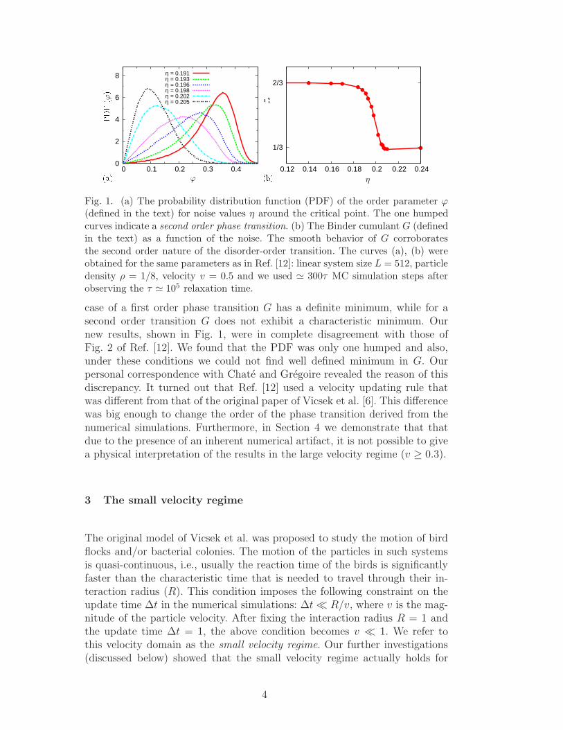
We re-investigated their simulations using the same parameters (system size L= 512, and particle velocity v = 0.5) and boundary conditions (periodic) theyimplemented. In particular, we were interested in obtaining the probabilitydistribution function (PDF) of the order parameter ϕ and also the pertainingBinder cumulant G. The Binder cumulant [14] defined as G = 1− < ϕ4 >/3 < ϕ2 >2 measures the fluctuations of the order parameter and is a goodmeasure to distinguish between first and second order phase transitions. In

3

2/3

1/3

0.12 0.14 0.16 0.18 0.2 0.22 0.24 0

2

4

6

8

0 0.1 0.2 0.3 0.4

η = 0.191η = 0.193η = 0.196η = 0.198η = 0.202η = 0.205

ϕ(a)PDF(ϕ) G

(b) η

Fig. 1. (a) The probability distribution function (PDF) of the order parameter ϕ(defined in the text) for noise values η around the critical point. The one humpedcurves indicate a second order phase transition. (b) The Binder cumulant G (definedin the text) as a function of the noise. The smooth behavior of G corroboratesthe second order nature of the disorder-order transition. The curves (a), (b) wereobtained for the same parameters as in Ref. [12]: linear system size L = 512, particledensity ρ = 1/8, velocity v = 0.5 and we used ≃ 300τ MC simulation steps afterobserving the τ ≃ 105 relaxation time.

case of a first order phase transition G has a definite minimum, while for asecond order transition G does not exhibit a characteristic minimum. Ournew results, shown in Fig. 1, were in complete disagreement with those ofFig. 2 of Ref. [12]. We found that the PDF was only one humped and also,under these conditions we could not find well defined minimum in G. Ourpersonal correspondence with Chate and Gregoire revealed the reason of thisdiscrepancy. It turned out that Ref. [12] used a velocity updating rule thatwas different from that of the original paper of Vicsek et al. [6]. This differencewas big enough to change the order of the phase transition derived from thenumerical simulations. Furthermore, in Section 4 we demonstrate that thatdue to the presence of an inherent numerical artifact, it is not possible to givea physical interpretation of the results in the large velocity regime (v ≥ 0.3).

3 The small velocity regime

The original model of Vicsek et al. was proposed to study the motion of birdflocks and/or bacterial colonies. The motion of the particles in such systemsis quasi-continuous, i.e., usually the reaction time of the birds is significantlyfaster than the characteristic time that is needed to travel through their in-teraction radius (R). This condition imposes the following constraint on theupdate time ∆t in the numerical simulations: ∆t ≪ R/v, where v is the mag-nitude of the particle velocity. After fixing the interaction radius R = 1 andthe update time ∆t = 1, the above condition becomes v ≪ 1. We refer tothis velocity domain as the small velocity regime. Our further investigations(discussed below) showed that the small velocity regime actually holds for

4

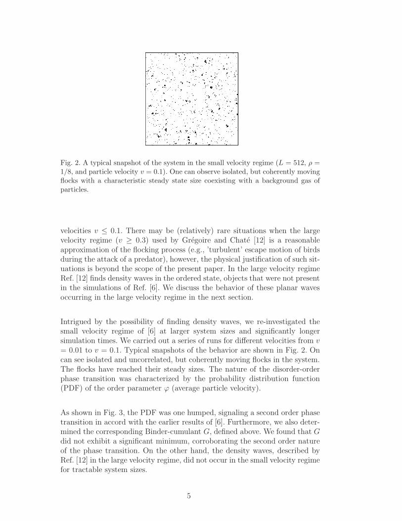
Fig. 2. A typical snapshot of the system in the small velocity regime (L = 512, ρ =1/8, and particle velocity v = 0.1). One can observe isolated, but coherently movingflocks with a characteristic steady state size coexisting with a background gas ofparticles.

velocities v ≤ 0.1. There may be (relatively) rare situations when the largevelocity regime (v ≥ 0.3) used by Gregoire and Chate [12] is a reasonableapproximation of the flocking process (e.g., ’turbulent’ escape motion of birdsduring the attack of a predator), however, the physical justification of such sit-uations is beyond the scope of the present paper. In the large velocity regimeRef. [12] finds density waves in the ordered state, objects that were not presentin the simulations of Ref. [6]. We discuss the behavior of these planar wavesoccurring in the large velocity regime in the next section.

Intrigued by the possibility of finding density waves, we re-investigated thesmall velocity regime of [6] at larger system sizes and significantly longersimulation times. We carried out a series of runs for different velocities from v= 0.01 to v = 0.1. Typical snapshots of the behavior are shown in Fig. 2. Oncan see isolated and uncorrelated, but coherently moving flocks in the system.The flocks have reached their steady sizes. The nature of the disorder-orderphase transition was characterized by the probability distribution function(PDF) of the order parameter ϕ (average particle velocity).

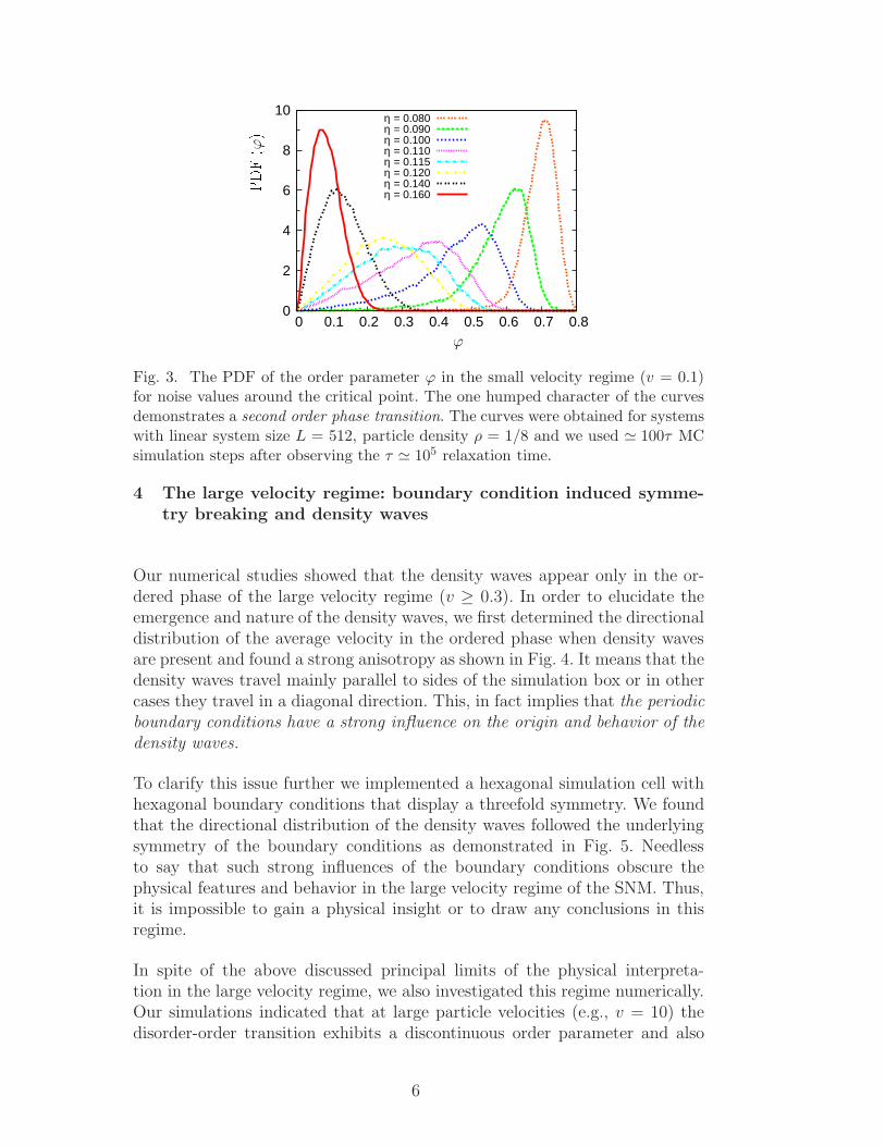
As shown in Fig. 3, the PDF was one humped, signaling a second order phasetransition in accord with the earlier results of [6]. Furthermore, we also deter-mined the corresponding Binder-cumulant G, defined above. We found that Gdid not exhibit a significant minimum, corroborating the second order natureof the phase transition. On the other hand, the density waves, described byRef. [12] in the large velocity regime, did not occur in the small velocity regimefor tractable system sizes.

5

0

2

4

6

8

10

0 0.1 0.2 0.3 0.4 0.5 0.6 0.7 0.8

η = 0.080η = 0.090η = 0.100η = 0.110η = 0.115η = 0.120η = 0.140η = 0.160

PDF(ϕ

)

ϕ

Fig. 3. The PDF of the order parameter ϕ in the small velocity regime (v = 0.1)for noise values around the critical point. The one humped character of the curvesdemonstrates a second order phase transition. The curves were obtained for systemswith linear system size L = 512, particle density ρ = 1/8 and we used ≃ 100τ MCsimulation steps after observing the τ ≃ 105 relaxation time.

4 The large velocity regime: boundary condition induced symme-try breaking and density waves

Our numerical studies showed that the density waves appear only in the or-dered phase of the large velocity regime (v ≥ 0.3). In order to elucidate theemergence and nature of the density waves, we first determined the directionaldistribution of the average velocity in the ordered phase when density wavesare present and found a strong anisotropy as shown in Fig. 4. It means that thedensity waves travel mainly parallel to sides of the simulation box or in othercases they travel in a diagonal direction. This, in fact implies that the periodic

boundary conditions have a strong influence on the origin and behavior of the

density waves.

To clarify this issue further we implemented a hexagonal simulation cell withhexagonal boundary conditions that display a threefold symmetry. We foundthat the directional distribution of the density waves followed the underlyingsymmetry of the boundary conditions as demonstrated in Fig. 5. Needlessto say that such strong influences of the boundary conditions obscure thephysical features and behavior in the large velocity regime of the SNM. Thus,it is impossible to gain a physical insight or to draw any conclusions in thisregime.

In spite of the above discussed principal limits of the physical interpreta-tion in the large velocity regime, we also investigated this regime numerically.Our simulations indicated that at large particle velocities (e.g., v = 10) thedisorder-order transition exhibits a discontinuous order parameter and also

6

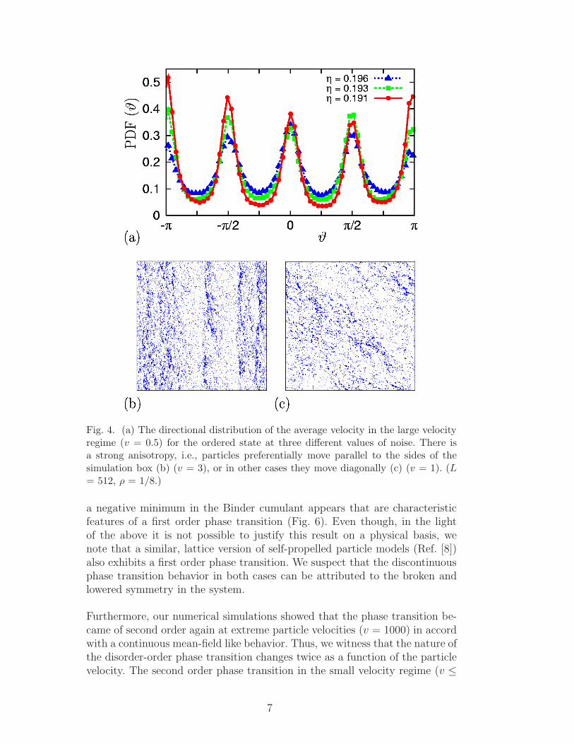
Fig. 4. (a) The directional distribution of the average velocity in the large velocityregime (v = 0.5) for the ordered state at three different values of noise. There isa strong anisotropy, i.e., particles preferentially move parallel to the sides of thesimulation box (b) (v = 3), or in other cases they move diagonally (c) (v = 1). (L= 512, ρ = 1/8.)

a negative minimum in the Binder cumulant appears that are characteristicfeatures of a first order phase transition (Fig. 6). Even though, in the lightof the above it is not possible to justify this result on a physical basis, wenote that a similar, lattice version of self-propelled particle models (Ref. [8])also exhibits a first order phase transition. We suspect that the discontinuousphase transition behavior in both cases can be attributed to the broken andlowered symmetry in the system.

Furthermore, our numerical simulations showed that the phase transition be-came of second order again at extreme particle velocities (v = 1000) in accordwith a continuous mean-field like behavior. Thus, we witness that the nature ofthe disorder-order phase transition changes twice as a function of the particlevelocity. The second order phase transition in the small velocity regime (v ≤

7

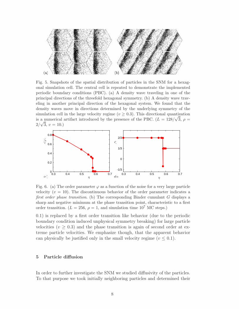
Fig. 5. Snapshots of the spatial distribution of particles in the SNM for a hexag-onal simulation cell. The central cell is repeated to demonstrate the implementedperiodic boundary conditions (PBC). (a) A density wave traveling in one of theprincipal directions of the threefold hexagonal symmetry. (b) A density wave trav-eling in another principal direction of the hexagonal system. We found that thedensity waves move in directions determined by the underlying symmetry of thesimulation cell in the large velocity regime (v ≥ 0.3). This directional quantizationis a numerical artifact introduced by the presence of the PBC. (L = 128/

√3, ρ =

2/√

3, v = 10.)

0

0.2

0.4

0.6

0.8

0.3 0.4 0.5 0.6 0.7

2/3

1/3

0

-1/3

0.3 0.4 0.5 0.6 0.7

<ϕ>

(a) (b)

G

ηη

Fig. 6. (a) The order parameter ϕ as a function of the noise for a very large particlevelocity (v = 10). The discontinuous behavior of the order parameter indicates afirst order phase transition. (b) The corresponding Binder cumulant G displays asharp and negative minimum at the phase transition point, characteristic to a firstorder transition. (L = 256, ρ = 1, and simulation time 107 MC steps.)

0.1) is replaced by a first order transition like behavior (due to the periodicboundary condition induced unphysical symmetry breaking) for large particlevelocities (v ≥ 0.3) and the phase transition is again of second order at ex-treme particle velocities. We emphasize though, that the apparent behaviorcan physically be justified only in the small velocity regime (v ≤ 0.1).

5 Particle diffusion

In order to further investigate the SNM we studied diffusivity of the particles.To that purpose we took initially neighboring particles and determined their

8

0

200

400

600

800

1000

0 2000 4000 6000 8000

0

200

400

600

800

1000

0 100 200 300

< r2(t) >

< r2⊥(t) >

< r2‖(t) >

<r

2 ij(t

)>

t t

< r2(t) >

< r2⊥(t) >

< r2‖(t) >

<r

2 ij(t

)>

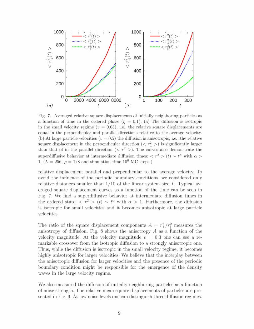
(a) (b)Fig. 7. Averaged relative square displacements of initially neighboring particles asa function of time in the ordered phase (η = 0.1). (a) The diffusion is isotropicin the small velocity regime (v = 0.05), i.e., the relative square displacements areequal in the perpendicular and parallel directions relative to the average velocity.(b) At large particle velocities (v = 0.5) the diffusion is anisotropic, i.e., the relativesquare displacement in the perpendicular direction (< r2

⊥ >) is significantly largerthan that of in the parallel direction (< r2

‖ >). The curves also demonstrate the

superdiffusive behavior at intermediate diffusion times: < r2 > (t) ∼ tα with α >1. (L = 256, ρ = 1/8 and simulation time 106 MC steps.)

relative displacement parallel and perpendicular to the average velocity. Toavoid the influence of the periodic boundary conditions, we considered onlyrelative distances smaller than 1/10 of the linear system size L. Typical av-eraged square displacement curves as a function of the time can be seen inFig. 7. We find a superdiffusive behavior at intermediate diffusion times inthe ordered state: < r2 > (t) ∼ tα with α > 1. Furthermore, the diffusionis isotropic for small velocities and it becomes anisotropic at large particlevelocities.

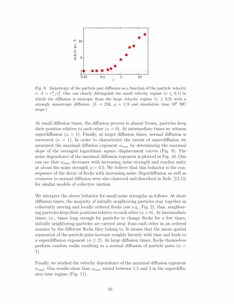
The ratio of the square displacement components A = r2

⊥/r2

‖ measures theanisotropy of diffusion. Fig. 8 shows the anisotropy A as a function of thevelocity magnitude. At the velocity magnitude v = 0.3 one can see a re-markable crossover from the isotropic diffusion to a strongly anisotropic one.Thus, while the diffusion is isotropic in the small velocity regime, it becomeshighly anisotropic for larger velocities. We believe that the interplay betweenthe anisotropic diffusion for larger velocities and the presence of the periodicboundary condition might be responsible for the emergence of the densitywaves in the large velocity regime.

We also measured the diffusion of initially neighboring particles as a functionof noise strength. The relative mean square displacements of particles are pre-sented in Fig. 9. At low noise levels one can distinguish three diffusion regimes.

9

10

5

1 0 0.01 0.1 1 10

v

Anisotropy,A

Fig. 8. Anisotropy of the particle pair diffusion as a function of the particle velocityv: A = r2

⊥/r2

‖. One can clearly distinguish the small velocity regime (v ≤ 0.1) in

which the diffusion is isotropic from the large velocity regime (v ≥ 0.3) with astrongly anisotropic diffusion. (L = 256, ρ = 1/8 and simulation time 106 MCsteps.)

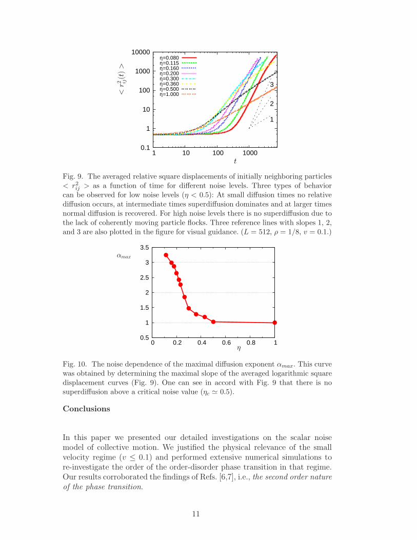
At small diffusion times, the diffusion process is almost frozen, particles keeptheir position relative to each other (α = 0). At intermediate times we witnesssuperdiffusion (α > 1). Finally, at larger diffusion times, normal diffusion isrecovered (α = 1). In order to characterize the extent of superdiffusion wemeasured the maximal diffusion exponent αmax by determining the maximalslope of the averaged logarithmic square displacement curves (Fig. 9). Thenoise dependence of the maximal diffusion exponent is plotted in Fig. 10. Onecan see that αmax decreases with increasing noise strength and reaches unityat about the noise strength η = 0.5. We believe that this behavior is the con-sequence of the decay of flocks with increasing noise. Superdiffusion as well ascrossover to normal diffusion were also observed and described in Refs. [12,15]for similar models of collective motion.

We interpret the above behavior for small noise strengths as follows. At shortdiffusion times, the majority of initially neighboring particles stay together incoherently moving and locally ordered flocks (see e.g., Fig. 2), thus, neighbor-ing particles keep their positions relative to each other (α = 0). At intermediatetimes, i.e., times long enough for particles to change flocks for a few times,initially neighboring particles are carried away from each other in an orderedmanner by the different flocks they belong to. It means that the mean spatialseparation of the particle pairs increase roughly linearly with time and leads toa superdiffusion exponent (α ≥ 2). At large diffusion times, flocks themselvesperform random walks resulting in a normal diffusion of particle pairs (α =1).

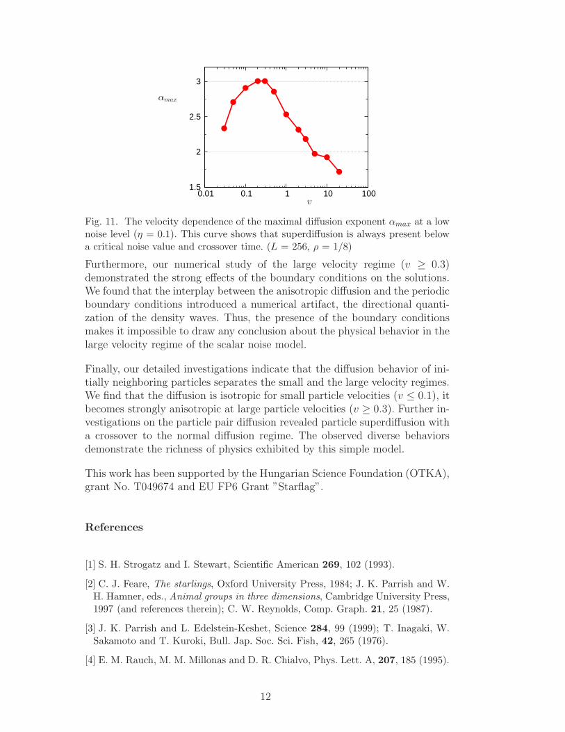
Finally, we studied the velocity dependence of the maximal diffusion exponentαmax. Our results show that αmax varied between 1.5 and 3 in the superdiffu-sion time regime (Fig. 11).

10

0.1

1

10

100

1000

10000

1 10 100 1000

1

2

3

η=0.080η=0.115η=0.160η=0.200η=0.300η=0.360η=0.500η=1.000<

r2 ij(t

)>

t

Fig. 9. The averaged relative square displacements of initially neighboring particles< r2

ij > as a function of time for different noise levels. Three types of behaviorcan be observed for low noise levels (η < 0.5): At small diffusion times no relativediffusion occurs, at intermediate times superdiffusion dominates and at larger timesnormal diffusion is recovered. For high noise levels there is no superdiffusion due tothe lack of coherently moving particle flocks. Three reference lines with slopes 1, 2,and 3 are also plotted in the figure for visual guidance. (L = 512, ρ = 1/8, v = 0.1.)

0.5

1

1.5

2

2.5

3

3.5

0 0.2 0.4 0.6 0.8 1η

αmax

Fig. 10. The noise dependence of the maximal diffusion exponent αmax. This curvewas obtained by determining the maximal slope of the averaged logarithmic squaredisplacement curves (Fig. 9). One can see in accord with Fig. 9 that there is nosuperdiffusion above a critical noise value (ηc ≃ 0.5).

Conclusions

In this paper we presented our detailed investigations on the scalar noisemodel of collective motion. We justified the physical relevance of the smallvelocity regime (v ≤ 0.1) and performed extensive numerical simulations tore-investigate the order of the order-disorder phase transition in that regime.Our results corroborated the findings of Refs. [6,7], i.e., the second order nature

of the phase transition.

11

1.5

2

2.5

3

0.01 0.1 1 10 100v

αmax

Fig. 11. The velocity dependence of the maximal diffusion exponent αmax at a lownoise level (η = 0.1). This curve shows that superdiffusion is always present belowa critical noise value and crossover time. (L = 256, ρ = 1/8)

Furthermore, our numerical study of the large velocity regime (v ≥ 0.3)demonstrated the strong effects of the boundary conditions on the solutions.We found that the interplay between the anisotropic diffusion and the periodicboundary conditions introduced a numerical artifact, the directional quanti-zation of the density waves. Thus, the presence of the boundary conditionsmakes it impossible to draw any conclusion about the physical behavior in thelarge velocity regime of the scalar noise model.

Finally, our detailed investigations indicate that the diffusion behavior of ini-tially neighboring particles separates the small and the large velocity regimes.We find that the diffusion is isotropic for small particle velocities (v ≤ 0.1), itbecomes strongly anisotropic at large particle velocities (v ≥ 0.3). Further in-vestigations on the particle pair diffusion revealed particle superdiffusion witha crossover to the normal diffusion regime. The observed diverse behaviorsdemonstrate the richness of physics exhibited by this simple model.

This work has been supported by the Hungarian Science Foundation (OTKA),grant No. T049674 and EU FP6 Grant ”Starflag”.

References

[1] S. H. Strogatz and I. Stewart, Scientific American 269, 102 (1993).

[2] C. J. Feare, The starlings, Oxford University Press, 1984; J. K. Parrish and W.H. Hamner, eds., Animal groups in three dimensions, Cambridge University Press,1997 (and references therein); C. W. Reynolds, Comp. Graph. 21, 25 (1987).

[3] J. K. Parrish and L. Edelstein-Keshet, Science 284, 99 (1999); T. Inagaki, W.Sakamoto and T. Kuroki, Bull. Jap. Soc. Sci. Fish, 42, 265 (1976).

[4] E. M. Rauch, M. M. Millonas and D. R. Chialvo, Phys. Lett. A, 207, 185 (1995).

12

[5] E. Ben-Jacob, I. Cohen, O. Shochet, A. Czirok and T. Vicsek, Phys. Rev. Lett.75, 2899 (1995); J. A. Shapiro, BioEssays 17, 597 (1995); J. A. Shapiro and M.Dworkin, eds., Bacteria as multicellular organisms, Oxford University Press, 1997.

[6] T. Vicsek, A. Czirok, E. Ben-Jacob, I. Cohen and O. Shochet Phys. Rev. Lett.75, 1226 (1995).

[7] A. Czirok, H. E. Stanley and T. Vicsek, J. Phys A 30, 1375 (1997).

[8] Z. Csahok and T. Vicsek, Phys. Rev. E 52, 5297 (1995).

[9] J. Toner and Y. Tu, Phys. Rev. Lett. 75, 4326 (1995).

[10] J. Toner, Y. Tu and M. Ulm, Phys. Rev. Lett. 80, 4819 (1998).

[11] J. Toner and Y. Tu, Phys. Rev. E 58, 4828 (1998).

[12] G. Gregoire and H. Chate, Phys. Rev. Lett. 92, 025702 (2004).

[13] C. Huepe and M. Aldana, Phys. Rev. Lett. 92, 168701 (2004).

[14] K. Binder and D. W. Herrmann, Monte Carlo Simulation in Statistical Physics,Springer (1997).

[15] G. Gregoire, H. Chate and Y. Tu, Phys. Rev. E 64, 011902 (2001); G. Gregoire,H. Chate and Y. Tu, Physica D 181, 157 (2003).

13