New Approaches for De–novo Motif Discovery Using ...

Page 1

New Approaches for De–novo Motif DiscoveryUsing Phylogenetic Footprinting:

From Data Acquisition to Motif Visualization

Dissertation

zur Erlangung des akademischen Grades

Doktor der Naturwissenschaften (Dr.rer.nat.)

der Naturwissenschaftliche Fakultät IIIAgrar- und Ernährungswissenschaften, Geowissenschaften und Informatik

der Martin-Luther-Universität Halle-Wittenberg

vorgelegt von

Arthur Martin NettlingGeb. am 10.06.1982 in Meerane

Gutachter:1. Prof. Dr. Ivo Grosse2. Prof. Dr. Peter Stadler

Tag der Verteidigung: 20. April 2017

Page 2

Page 3

Page 4

ii

Page 5

Acknowledgements

First of all, I thank my beloved wife, Jasmin Nettling, and my whole family for the greatsupport and the patience during the last years. Thank you very much for watching thekids when there was a deadline. Thank you for serving coffee, food, and beer, when I hadno time to join lunch or the family party. And thank you for letting me sleep the daywhen I worked all night again. I am very grateful to my supervisor, adviser, and friendIvo Grosse, who guided me through my Ph.D. studies. I value very much our honest andpassionate discussions at every day or night.

I am also very grateful for the interesting and goal-oriented discussions with HendrikTreutler. Thank you very much for reading almost everything I have written, for yourvaluable and honest comments, and your motivating words when evolution behaved againunexpected and unwished.

Further, I thank Andreas Both, Karin Breunig, Jesus Cerquides, Ralf Eggeling, Jan Grau,Jens Keilwagen, Konstantin Kruse, Stefan Posch, Yvonne Pöschel, Marcel Quint, PeterStadler, and Martin Staege for the valuable discussions, for keeping me on track, and forgiving me advice in nearly every Ph.D. related problem. Jan and Jens, you do a reallygreat job with Jstacs (http://www.jstacs.de). Thank you very much for your kind andfast support every time.

And last but not least, I thank Jörg Weber for helping to develop and implement theweb-server http://difflogo.com and Charles Bishop for proofreading this thesis.

iii

Page 6

iv

Page 7

Peer-reviewed publications

This thesis is a cumulative thesis based on the following publications.

• P Alexiou, T Vergoulis, M Gleditzsch, G Prekas, T Dalamagas, M Megraw, I Grosse, TSellis, AG Hatzigeorgiou. 2009. miRGen 2.0: a database of microRNA genomic informationand regulation.Nucl. Acids Res. 38 (suppl 1): D137-D141 . doi:10.1093/nar/gkp888

• M Nettling, N Thieme, A Both, I Grosse. 2014. DRUMS: Disk Repository with UpdateManagement and Select option for high throughput sequencing data.BMC bioinformatics, 15:1. doi:10.1186/1471-2105-15-38

• M Nettling, H Treutler, J Cerquides, I Grosse. 2016. Detecting and correcting the binding-affinity bias in ChIP-Seq data using inter-species information.BMC Genomics 17:1. doi:10.1186/s12864-016-2682-6

• M Nettling, H Treutler, J Cerquides, I Grosse. 2017. Unrealistic phylogenetic trees mayimprove phylogenetic footprinting.Bioinformatics doi: 10.1093/bioinformatics/btx033

• M Nettling, H Treutler, J Cerquides, I Grosse. 2017. Combining phylogenetic footprintingwith motif models incorporating intra-motif dependencies.BMC Bioinformatics, 18:141 doi: 10.1186/s12859-017-1495-1

• M Nettling*, H Treutler*, J Grau, J Keilwagen, S Posch, I Grosse. 2015. DiffLogo: acomparative visualization of sequence motifs.BMC bioinformatics, 16:1 doi:10.1186/s12859-015-0767-x

I hereby declare that the copyright of the content of the articles Alexiou et al., 2009 andNettling et al., 2017b is by Oxford University Press. These papers are available at:

• http://nar.oxfordjournals.org/content/38/suppl_1/D137

• https://academic.oup.com/bioinformatics/article/2959846

I hereby declare that the copyright of the content of the articles Nettling, Thieme, et al.,2014, Nettling, Treutler, Grau, et al., 2015, Nettling et al., 2016, and Nettling et al., 2017ais by the authors. These papers are available at:

• http://bmcbioinformatics.biomedcentral.com/articles/10.1186/1471-2105-15-38

• http://bmcbioinformatics.biomedcentral.com/articles/10.1186/s12859-015-0767-x

• http://bmcgenomics.biomedcentral.com/articles/10.1186/s12864-016-2682-6

• https://bmcbioinformatics.biomedcentral.com/articles/10.1186/s12859-017-1495-1

v

Page 8

vi

Page 9

Contents

1 Summary 11.1 English version . . . . . . . . . . . . . . . . . . . . . . . . . . . . . . . . . . 11.2 German version . . . . . . . . . . . . . . . . . . . . . . . . . . . . . . . . . . 4

2 Introduction 72.1 Biological background . . . . . . . . . . . . . . . . . . . . . . . . . . . . . . 8

2.1.1 Gene expression and gene regulation . . . . . . . . . . . . . . . . . . 82.1.2 Transcriptional initiation . . . . . . . . . . . . . . . . . . . . . . . . 92.1.3 Gene regulation by miRNAs . . . . . . . . . . . . . . . . . . . . . . . 10

2.2 Computer science background . . . . . . . . . . . . . . . . . . . . . . . . . . 112.2.1 The Java programming language and the Java library Jstacs . . . . 112.2.2 The R programming language and Bioconductor . . . . . . . . . . . 122.2.3 Databases . . . . . . . . . . . . . . . . . . . . . . . . . . . . . . . . . 13

2.3 Bioinformatics background . . . . . . . . . . . . . . . . . . . . . . . . . . . . 142.3.1 Integration of biological data . . . . . . . . . . . . . . . . . . . . . . 142.3.2 ChIP-seq data analysis . . . . . . . . . . . . . . . . . . . . . . . . . . 152.3.3 De–novo motif discovery based on phylogenetic footprinting . . . . . 162.3.4 visualization of sequence motifs . . . . . . . . . . . . . . . . . . . . . 18

2.4 Research objectives . . . . . . . . . . . . . . . . . . . . . . . . . . . . . . . . 18

3 Context of publications 213.1 Data acquisition and data preparation . . . . . . . . . . . . . . . . . . . . . 22

3.1.1 miRGen 2.0: a database of microRNA genomic information and reg-ulation . . . . . . . . . . . . . . . . . . . . . . . . . . . . . . . . . . . 23

3.1.2 DRUMS: Disk Repository with Update Management and Select op-tion for high throughput sequencing data . . . . . . . . . . . . . . . 25

3.2 Predicting transcription factor binding sites using phylogenetic footprinting . 273.2.1 Detecting and correcting the binding-affinity bias in ChIP-Seq data

using inter-species information . . . . . . . . . . . . . . . . . . . . . 283.2.2 Unrealistic phylogenetic trees may improve phylogenetic footprinting 303.2.3 Combining phylogenetic footprinting with motif models incorporat-

ing intra-motif dependencies . . . . . . . . . . . . . . . . . . . . . . . 333.3 Visualization of sequence motifs . . . . . . . . . . . . . . . . . . . . . . . . . 35

3.3.1 DiffLogo: A comparative visualization of sequence motifs . . . . . . 35

vii

Page 10

CONTENTS

3.3.2 WebDiffLogo: A web-server for the construction and visualization ofmultiple motif alignments . . . . . . . . . . . . . . . . . . . . . . . . 37

3.4 Conclusions and outlook . . . . . . . . . . . . . . . . . . . . . . . . . . . . . 40

4 Data acquisition and data preparation 554.1 miRGen 2.0: a database of microRNA genomic information and regulation . 554.2 DRUMS: Disk Repository with Update Management and Select option . . . 61

5 Predicting transcription factor binding sites using Phylogenetic Foot-printing 715.1 Detecting and correcting the binding-affinity bias in ChIP-Seq data using

inter-species information . . . . . . . . . . . . . . . . . . . . . . . . . . . . . 715.2 Unrealistic phylogenetic trees may improve phylogenetic footprinting . . . . 825.3 Combining phylogenetic footprinting with motif models incorporating intra-

motif dependencies . . . . . . . . . . . . . . . . . . . . . . . . . . . . . . . . 93

6 Visualisation of motifs 1036.1 DiffLogo: A comparative visualisation of sequence motifs . . . . . . . . . . . 103

7 Appendix 1137.1 Detecting and correcting the binding-affinity bias in ChIP-Seq data using

inter-species information . . . . . . . . . . . . . . . . . . . . . . . . . . . . . 1137.1.1 Modeling the binding-affinity bias . . . . . . . . . . . . . . . . . . . . 113

7.2 Unrealistic phylogenetic trees may improve phylogenetic footprinting . . . . 1167.2.1 Accuracy of predicted motifs . . . . . . . . . . . . . . . . . . . . . . 1167.2.2 Synthetic tests . . . . . . . . . . . . . . . . . . . . . . . . . . . . . . 118

7.3 Combining phylogenetic footprinting with motif models incorporating intra-motif dependencies . . . . . . . . . . . . . . . . . . . . . . . . . . . . . . . . 1277.3.1 Species–specific motifs are highly similar for most TF . . . . . . . . 1277.3.2 Taking into account phylogeny improves classification performance

in almost all cases. . . . . . . . . . . . . . . . . . . . . . . . . . . . . 1337.4 DiffLogo: A comparative visualisation of sequence motifs . . . . . . . . . . . 137

7.4.1 Alternative combinations of stack heights and symbol weights . . . . 137

viii

Page 11

1 Summary

1.1 English version

The versatility of organisms and their adaptability to environmental changes are essentialfor their viability and are achieved by expressing proteins on demand. The expression ofproteins is orchestrated by the process of gene regulation, which belong to the most complexand comprehensive processes in nature. Hence, the understanding of gene regulation is aprerequisite in modern biology, medicine, and, biodiversity research. A crucial sub-processin gene regulation is the transcriptional initiation, i.e., the interaction of transcriptionfactors (TFs) with their transcription factor binding sites (TFBSs). Hence, predictingTFBSs and their binding motifs in biological sequences is essential for the understandingof gene regulation.

Identifying TFBSs and binding motifs using wet-lab experiments is expensive and time-consuming, and thus neither economical nor feasible. Consequently, bioinformatics ap-proaches have been developed for, first, data acquisition and data preparation, second,for the prediction of putative TFBSs on genomic scale, and third, for the visualization ofmodels for TFBSs.

A typical task in bioinformatics covering these three fields is the prediction of TFBSs inChIP-sequencing (ChIP-seq) data. This task starts with obtaining sequence data directlyfrom a ChIP-seq experiment or some database. After transforming the data into an ap-propriate format, de-novo motif discovery is performed and putative TFBSs are predicted.Finally, the results are visualized and compared to related work. This thesis covers sixpeer reviewed articles and one work-in-progress article, which fit into the mentioned threefields as follows.

First, demanded by business and academic needs, the number of data-intensive processesin bioinformatics, like next generation sequencing, is continuously increasing and so is theamount of produced data. The post-processing of these data increases this amount evenfurther. By combining various data sources and different types of data, like sequence datawith gene expression data, the data to manage becomes more and more complex. Hence,new databases are needed for an appropriate handling of complex data and new conceptsare needed for an efficient handling of increasingly large data volumes.

My colleagues and I developed miRGen, a relational MySQL database that stores mi-croRNA (miRNA) transcripts with target genes, contained single nucleotide polymor-

1

Page 12

1. SUMMARY

phisms (SNPs), TFBSs in near distance, and prominent literature sources. Over thelast years, miRGen has already become an important resource for researchers that areinterested in miRNA regulation and miRNA function.

We also developed the open-source Java libarary DRUMS which is designed to store bil-lions of position specific DNA related records. DRUMS is capable of performing fastand resource sparing requests and runs on a single standard computer. When comparingDRUMS to the standard database MySQL regarding insert performance and lookup per-formance on two data sets, it outperforms MySQL by a factor of two up to a factor of15456.

Second, predicting TFBSs in sequence data is essential for the understanding of gene reg-ulation and dozens of bioinformatics approaches have been developed for the predictionof TFBSs. These approaches use diverse statistical characteristics to distinguish TFBSsfrom their flanking Deoxyribonucleic acid (DNA) and can be subdivided in phylogeneticand non-phylogenetic approaches. Phylogenetic approaches take into account phylogeneticdependencies in aligned sequences of more than one species whereas non-phylogenetic ap-proaches based on sequences of only one species typically take into account intra-motifdependencies. The articles comprising this thesis are related to de-novo motif discoveryusing phylogenetic approaches as follows.

We extended a traditional phylogenetic footprinting model (PFM) by the capability totake into account the binding affinity bias (BA bias) in ChIP-seq data. The BA bias isa result of the over-representation of high-scoring binding sites in ChIP-seq data, causingthe inference of potentially distorted motifs. My colleagues and I found that correctingthe binding-affinity bias typically leads to softened motifs and significantly improves motifprediction.

We further studied the influence of phylogenetic trees on the performance of phylogeneticfootprinting and motif prediction. We surprisingly found that unrealistic phylogenetic treesoften lead to more accurate predictions of TFBSs than realistic phylogenetic trees.

Based on these results, we developed an approach for de-novo motif discovery that extendsphylogenetic footprinting by the capability of taking into account intra-motif dependenciesof higher order. My colleagues and I found intra-motif dependencies of order 1 and 2 inmotifs of all investigated species and we found that modelling intra-motif dependencieswithin phylogenetic footprinting significantly improves classification performance.

Third, visualizing the results of motif discovery is fundamental for researchers to interpret,present, and share their findings and sequence logos are the de facto standard in biologyand bioinformatics to accomplish this task. The number of data sets and motif extractionalgorithms is continuously growing and therefor the number of published motifs. Hence,it is often not sufficient to just show motifs but it becomes more and more important

2

Page 13

1.1 English version

to perceive differences between motifs. Comparing multiple sequence motifs by visualinspection of the corresponding sequence logos can be tricky and especially differences ofmultiple motifs of the same TF are often hard to perceive.

To address this problem my colleagues and I developed DiffLogo, an R-package that isspecifically designed for visualizing differences between similar sequence motifs. DiffLogovisualizes differences between multiple motifs in a tabular plot of all pairwise comparisons.The resulting matrix guides the viewer to the most prominent pairwise differences be-tween motifs. DiffLogo is already used in several articles of this thesis to depict differencesbetween motifs of the same TF from phylogenetically related species and to depict differ-ences between motifs of the same TF but captured by different de-novo motif discoveryapproaches.

We know that not all researchers have access to hardware with R and DiffLogo installed andnot all researchers have the time or the technical background to use R and DiffLogo withouthigh effort. Hence, we integrated DiffLogo into the web-server WebDiffLogo accessible viahttp://difflogo.com. This web-server allows the user to upload motifs in several commonformats. Further, WebDiffLogo allows the user to upload motifs of different length andorientation. Hence, WebDiffLogo is much easier to use and thus applicable to a muchlarger community.

Taken together, the findings of this thesis may advance our understanding of transcriptionalgene regulation and its evolution. Specifically, our work in the field of data acquisition anddata preparation may improve knowledge transfer among researchers and data handling.Our findings in the field of de–novo motif discovery based on phylogenetic footprintingmay lead to an improved prediction of TFBSs. Our work in the field of comparative motifvisualisation may help researchers regarding decision making, knowledge sharing, and thepresentation of results.

3

Page 14

1. SUMMARY

1.2 German version

Die Vielseitigkeit existierender Lebewesen und die Anpassungsfähigkeit an ihre Umwelt isteine Grundlage für das Leben selbst und ist nur möglich durch die bedarfsbedingte Expres-sion von Proteinen. Die Expression von Proteinen wird durch den Prozess der Genregula-tion gesteuert, wobei die Genregulation selbst zu den komplexesten und umfangreichstenProzessen in der Natur zählt. Folglich ist das Verständnis des Genregulationsprozessessowohl für biologische und medizinische Forschung, als auch für Forschung im Bereichder Biodiversität unabdingbar. Ein entscheidender Teilprozess der Genregulation ist dietranskriptionelle Initiation, mit anderen Worten, die Interaktion von Transkriptionsfak-toren (TFen) mit den korrespondierenden Transkriptionsfaktorbindestellen (TFBSen). DieVorhersage von TFBSen und die Inferenz ihrer Bindemotive ist somit eine unabdingbareGrundlage um den gesamten Prozess der Genregulation zu verstehen.

Die Identifikation von TFBSen und ihren Bindemotiven mittels klassischer Laborexperi-mente ist jedoch teuer und zeitaufwändig und damit weder ökonomisch noch praktikabel.Folglich wurden bioinformatische Methoden und Ansätze entwickelt, um Daten effizientzu beschaffen und vor zu verarbeiten, um mögliche TFBSen genomweit vorherzusagen undum Modelle für TFBSen zu visualisieren.

Eine typische bioinformatische Aufgabe, welche diese drei Bereiche umfasst, ist die Vorher-sage von TFBSen in ChIP-seq Daten. Diese Aufgabe beginnt mit der Akquisition vonSequenzdaten entweder direkt aus einem ChIP-seq Experiment oder aus entsprechen-den Datenbanken. Nachdem die Daten aufbereitet und in ein passendes Format trans-formiert wurden, kann die eigentliche Motivvorhersage beginnen. Abschließend werden dieErgebnisse typischerweise visualisiert und mit denen ähnlicher Arbeiten verglichen. Dievorliegende Dissertation umfasst sechs begutachtete Publikationen und ein Manuskript,welches noch in Arbeit ist, die sich folgendermaßen in die genannten drei Bereiche einglie-dern.

Erstens, aufgrund industriellen und akademischen Bedarfs steigt die Zahl der dateninten-siven Prozesse in der Bioinformatik an. Ein Beispiel dafür ist Next Generation Sequencing.In gleichem Maße wächst der Umfang produzierter Daten. Die Nachverarbeitung dieserDaten steigert die Datenmenge nochmals. Des Weiteren wird durch die Kombination ver-schiedener Datenquellen und Datentypen, wie Sequenzdaten und Expressionsdaten, dieKomplexität der zu verwaltenden Daten stetig erhöht. Damit steigt der Bedarf an neuenDatenbanken, die in der Lage sind, komplexere Daten zu verwalten. Außerdem werdenneue Konzepte benötigt um die immer größer werdenden Datenmengen effizient verwaltenzu können.

4

Page 15

1.2 German version

In diesem Kontext haben meine Kollegen und ich miRGen entwickelt, eine relationaleMySQL Datenbank zur Speicherung von microRNA (miRNA) Transkripten, angereichertmit deren Zielgenen, mit enthaltenen Einzelnukleotid-Polymorphismen (SNPs), mit TFBS-en in direkter Umgebung und mit prominenten Literaturquellen. miRGen ist bereits zueiner wichtigen Ressource für Forscher geworden, die an der Regulation und der Funktionvon miRNAs interessiert sind.

Des Weiteren haben wir die open-source Java Bibliothek DRUMS zur Speicherung von Mil-liarden von Datensätzen entwickelt, welche sich positionsspezifisch auf Sequenzen beziehen,wie es bei z. B. SNPs der Fall ist. DRUMS ist in der Lage Anfragen schnell undressourcenschonend zu beantworten und läuft auf Standard-Desktop-Hardware. Bei demVergleich von DRUMS mit der Standarddatenbanklösung MySQL bezüglich Einfügege-schwindigkeit und Anfragegeschwindigkeit istDRUMS 2 bis 15456mal schneller alsMySQL.

Zweitens, die Vorhersage von TFBSen in Sequenzdaten ist unabdingbar für das Verständ-nis des Genregulationsprozesses. Dutzende bioinformatische Ansätze existieren, um dieszu bewerkstelligen. Diese Ansätze nutzen verschiedene statistische Eigenschaften, umTFBSen von flankierender DNA zu unterscheiden. Phylogenetische Ansätze verwendenphylogenetische Abhängigkeiten in alignierten Sequenzen mehrerer Spezies, wohingegennicht-phylogenetische Ansätze basierend auf Sequenzen von nur einer Spezies normaler-weise Nukleotidabhängigkeiten innerhalb des Motivs berücksichtigen können. Die Arbeitendieser Dissertation sind fokussiert auf die Motiverkennung unter Verwendung phylogene-tischer Ansätze.

In diesem Kontext haben wir als Erstes ein traditionelles Phylogenetic Footprinting Modellum die Fähigkeit erweitert den Bindeaffinitätsbias (BA bias) von TFen in ChIP-seq Datenzu berücksichtigen. Der BA bias resultiert aus der Überrepräsentation von hochqualitativenBindestellen in ChIP-seq Daten und verursacht die Vorhersage von potentiell verzerrtenMotiven. Wir konnten zeigen, dass das Korrigieren des BA bias in der Regel zu weicherenMotiven führt und die Motivvorhersage signifikant verbessert.

Des Weiteren haben meine Kollegen und ich den Einfluss phylogenetischer Bäume auf dieLeistung von Phylogenetic Footprinting und Motivvorhersage untersucht. Überraschender-weise haben wir entdeckt, dass unrealistische phylogenetische Bäume oftmals zu genauerenVorhersagen von TFBSen führen als realistische phylogenetische Bäume.

Aufbauend auf dieser Erkenntnis haben wir einen Ansatz zur Motiverkennung entwickelt,welcher Phylogenetic Footprinting um die Fähigkeit erweitert Nukleotidabhängigkeitenhöherer Ordnung innerhalb eines Motivs zu modellieren. Wir haben Nukleotidabhängig-keiten erster und zweiter Ordnung in Motiven aller untersuchten Spezies gefunden undwir konnten zeigen, dass das Modellieren von Nukleotidabhängigkeiten im Rahmen vonPhylogenetic Footprinting die Vorhersagegüte signifikant verbessert.

5

Page 16

1. SUMMARY

Drittens, die Visualisierung der Modelle, die während der Motiverkennung generiert werdenist für Wissenschaftler fundamental um zum einen ihre Ergebnisse selbst interpretieren zukönnen und zum anderen um Erkenntnisse zu präsentieren und zu teilen. In vielen Be-reichen der Biologie und Bioinformatik werden dafür Sequenzlogos verwendet. Durch diestetig steigende Zahl an verfügbaren Datensätzen und Algorithmen zur Motiverkennungwächst die Zahl der veröffentlichten Sequenzmotive. Damit ist es oft nicht mehr aus-reichend Sequenzmotive lediglich zu präsentieren bzw. zu visualisieren, sondern es wirdimmer wichtiger auch Unterschiede zwischen Sequenzmotiven hervorzuheben. Der Ver-gleich mehrere Sequenzmotive mittels Sequenzlogos kann sich als äußerst schwierig erweisenund im Besonderen ist es auf diese Weise kaum möglich Unterschiede zwischen Motivendes gleichen TFs aus z. B. unterschieldichen Zelllinien zu erkennen.

Meine Kollegen und ich haben dieses Problem mit der Entwicklung von DiffLogo adressiert,ein speziell für die Visualisierung von Motivunteschieden entwickeltes R-Paket. DiffLogo vi-sualisiert Unterschiede mehrerer Motive in einer tabellarischen Darstellung aller paarweisenVergleiche. Die resultierende Visualisierung hebt prominente, paarweise Unterschiede farb-lich hervor und fokussiert somit den Betrachter auf das Wesentliche. DiffLogo wird bereitsin mehreren Publikationen dieser Dissertation verwendet.

Da nicht alle Wissenschaftler Zugang zu entsprechender Hardware mit installiertem R undDiffLogo haben und außerdem viele Wissenschaftler nicht genügend Zeit oder technischeErfahrung haben um R und DiffLogo ohne Probleme zu verwenden, haben wir DiffLogo ineinen WebServer integriert. Dieser ist über http://difflogo.com erreichbar. Der Nutzerkann Sequenzmotive in verschiedenen Formaten hochladen. Außerdem dürfen die Motiveunterschiedlich lang sein und eine unterschiedliche Orientierung haben. DiffLogo versuchtin diesen Fällen die Sequenzmotive zu alignieren. http://difflogo.com ist wesentlich ein-facher zu verwenden als DiffLogo und damit für eine größere Nutzerschaft zugänglich.

Abschließend kann ich sagen, dass die Erkenntnisse dieser Arbeit unser Verständnis dertranskriptionellen Genregulation und deren Evolution voranbringen können. Im Detail:Unsere Arbeit und unsere Erkenntnisse im Bereich der Datenakquisition und Datenvorbe-reitung können den Wissenstransfer zwischen Wissenschaftlern und das allgemeine Daten-management verbessern. Unsere Erkenntnisse im Bereich der Motivvorhersage mittelsPhylogenetic Footprinting können zu einer verbesserten Vorhersage von TFBS führen.Unsere Arbeit im Bereich der vergleichenden Darstellung von Sequenzmotiven kann Wis-senschaftlern bei der Entscheidungsfindung, beim Wissenstranfer, bei der Dokumentationund Präsentation ihrer Ergebnisse helfen.

6

Page 17

2 IntroductionFrom 1857 to 1864, Gregor Mendel studied the inheritance patterns in pea plants andsuggested the idea of the existence of discrete inheritable units. At the same time Darwinpublished his famous work “On the Origin of Species,” proposing continual evolution ofspecies (Darwin, 1859). It took over 50 years (1909) until Wilhelm Johannsen coined theword gene to name those inheritable units proposed by Mendel, and it took another 44years before James Watson and Francis Crick published their model for DNA, which is nowknown as the double-helix model of DNA structure (Watson et al., 1953). Three years later,Francis Crick stated the central dogma of molecular biology for the first time. Thisdogma describes the relationship between DNA, Ribonucleic acid (RNA), and proteins andwas finally published in 1970 (F. Crick et al., 1970). Ever since then, molecular biology hasundergone a rapid and extensive development and after 150 years, terms like gene, DNA,RNA, proteins, evolution, and mutation have found its way into our daily language.

This development was accompanied by the digital revolution, starting with the inventionof the transistor in 1947, the fundamental building block of any modern digital device.In the 70s, home computers were introduced and the transformation of analog to digitaldata began. In 1969 the first message was sent over the ARPANET, the predecessor of theInternet, which became publicly accessible in 1991 as the World Wide Web. Nowadays,50% of the world population has access to the Internet1 and everybody is passively andactively generating data that can be used to improve our daily lives. For example, GPSdata of many individuals can be used to predict traffic anomalies (Pang et al., 2013), dataof fitness trackers can be used to prevent cardiovascular diseases (Neubeck et al., 2015), anddifferences in human genomes can be used to understand the genetic contribution to variousdiseases (E. P. Consortium et al., 2012; 1. G. P. Consortium et al., 2012; Sudmant et al.,2015). It is expected that in 2020 the digital universe will comprise over 5, 200 gigabytesper living person, summing up to 40 trillion gigabytes of data (Gantz et al., 2012; Dragland,2013). The continuously growing quantity of information and its availability at any time,in any place, already permeates both our work and our daily lives.

The digital revolution also enabled new data sources and new technologies in the field ofmolecular biology, e.g., sequence data and sequencing technologies. Starting in 1990, ittook 13 years to sequence the first human genome, whereas in 2015, this task could beaccomplished in 26 hours (Miller et al., 2015). The extensive and continuously growingamount of data enabled the emergence of new sciences like bioinformatics, unleashing

1http://www.internetworldstats.com/stats.htm

7

Page 18

2. INTRODUCTION

new potentials regarding the study of fundamental biological processes like the complexprocess of gene regulation. Nowadays, molecular biology is a field of research that serves abroad audience with a scientific background as well as non-scientific backgrounds. In thissense, with this thesis, I want to contribute to a deeper understanding of the process ofgene regulation and its evolution. Specifically, my colleagues and I try to contribute todata acquisition and data preparation by developing new databases for knowledge sharingand for efficient data handling. We also attempt to develop new approaches based onphylogenetic footprinting for the de–novo motif discovery in ChIP-seq data. Finally, we tryto develop a new approach for the comparative visualization of sequence motifs. The nextfour sections introduce the reader to molecular biology, computer science, bioinformatics,and the research objectives of this thesis.

2.1 Biological background

This section gives a general introduction into gene expression and gene regulation. Theintroduction also includes a description of the transcriptional initiation and the post–transcriptional gene regulation by miRNAs.

2.1.1 Gene expression and gene regulation

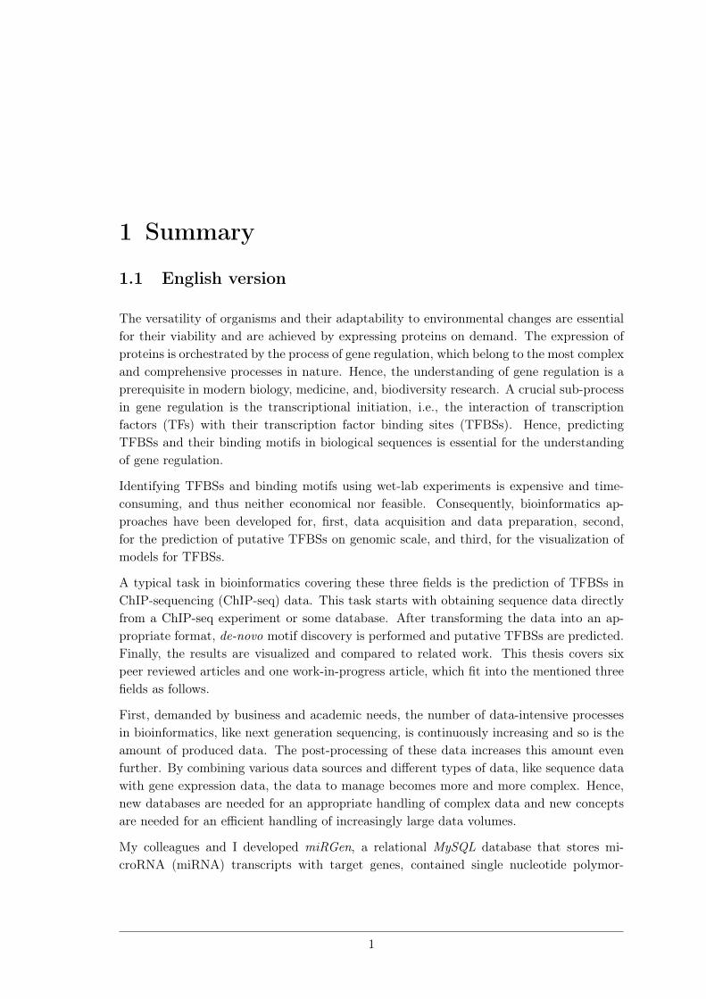
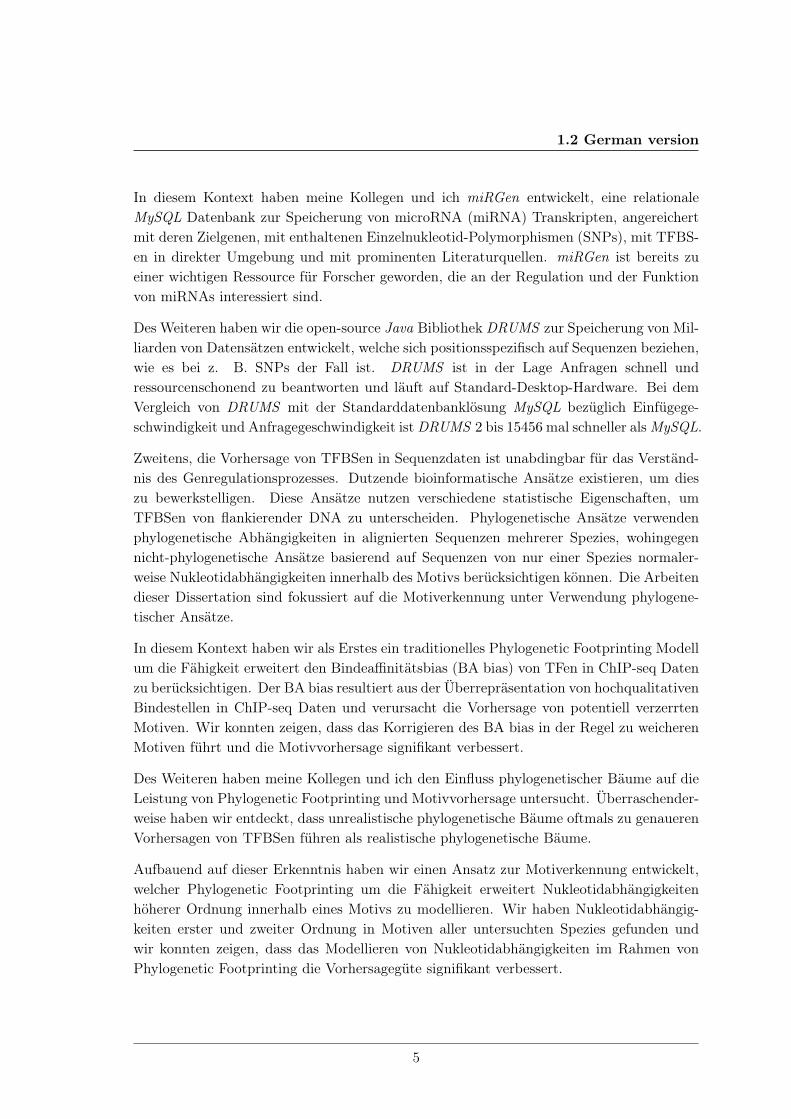
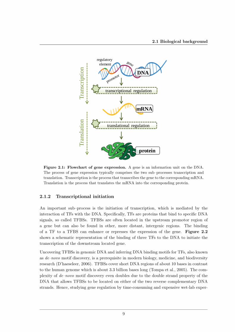
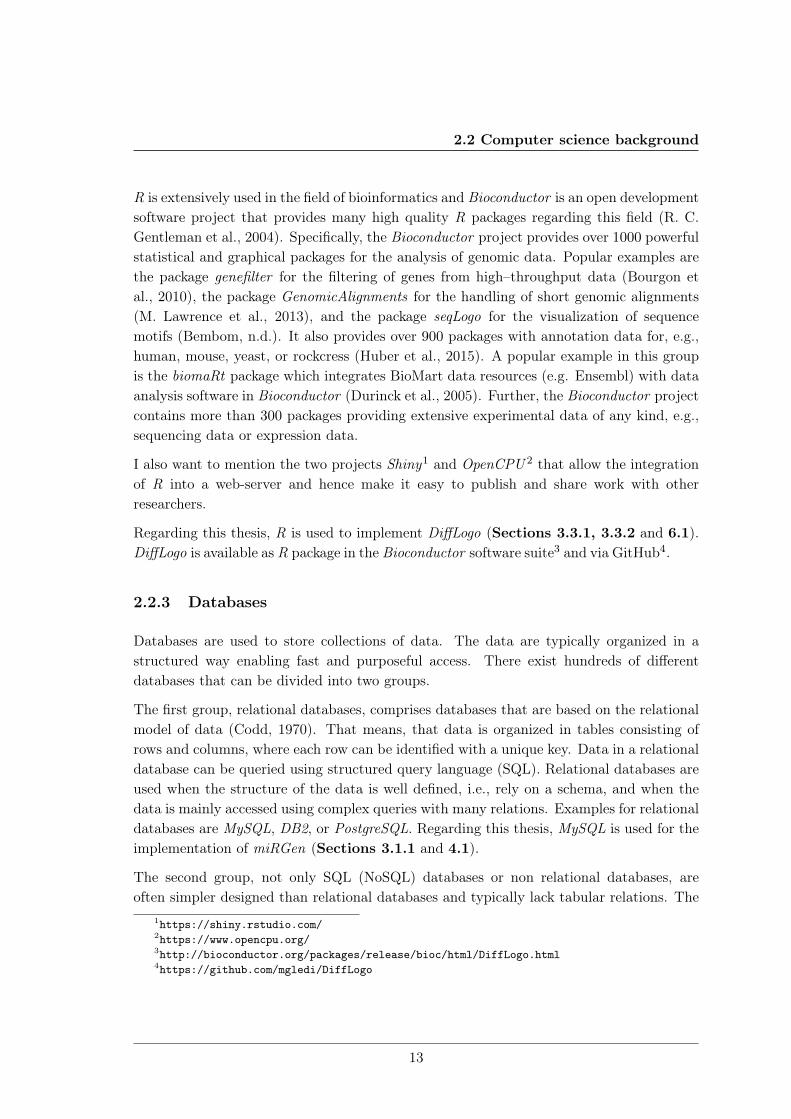
DNA is the intra–cellular substance that carries the definition of an organism’s potentials.It is composed of the nucleotides of the four organic bases adenine (A), cytosine (C ), gua-nine (G), and thymine (T ). The sequence of these bases encodes the genetic information.Genes are information units on the DNA and gene expression is the process used by allknown life that translates genes into proteins or functional RNA. In all organisms, geneexpression comprises at least two processes, transcription and translation (Figure 2.1).Transcription is the process that transcribes a DNA sequence to the corresponding mes-senger RNA (mRNA) sequence. Translation is the process that translates the mRNA intothe corresponding polypeptide, which may then fold to a protein.

Gene regulation is the process that regulates gene expression and is the basis for cellulardifferentiation, morphogenesis, versatility, and adaptability of any organism. Whenever aprotein is needed, due to e.g., environmental stimuli, a complex signaling cascade is initi-ated to first, make the corresponding DNA region accessible for the transcription machineryand second, to ensure the correct processing of the genetic information. This fundamentalprocess is established by diverse sub–processes such as epigenetics (Reik, 2007; Slotkinet al., 2007; Dolinoy et al., 2007), regulation by miRNAs (He et al., 2004; K. Chen etal., 2007), siRNA interference (Fougerolles et al., 2007; Tam et al., 2008), and alternativesplicing (Sultan et al., 2008; Luco et al., 2010).

8

Page 19

2.1 Biological background

regulatory

element

DNA

mRNA

protein

transcriptional regulation

Tra

nsc

rip

tio

n

Tra

nsl

atio

n

translational regulation

Figure 2.1: Flowchart of gene expression. A gene is an information unit on the DNA.The process of gene expression typically comprises the two sub–processes transcription andtranslation. Transcription is the process that transcribes the gene to the corresponding mRNA.Translation is the process that translates the mRNA into the corresponding protein.

2.1.2 Transcriptional initiation

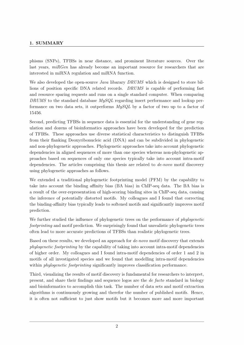
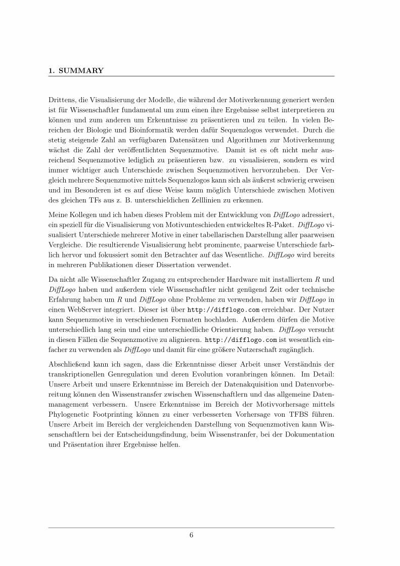
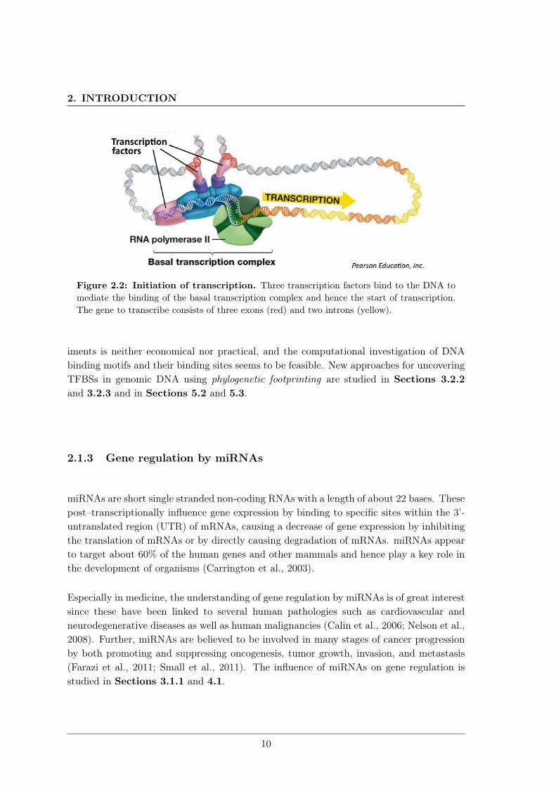
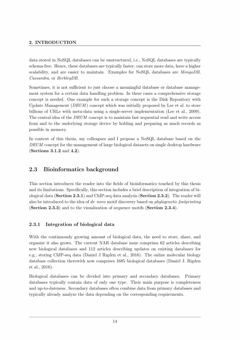
An important sub–process is the initiation of transcription, which is mediated by theinteraction of TFs with the DNA. Specifically, TFs are proteins that bind to specific DNAsignals, so called TFBSs. TFBSs are often located in the upstream promotor region ofa gene but can also be found in other, more distant, intergenic regions. The bindingof a TF to a TFBS can enhance or represses the expression of the gene. Figure 2.2shows a schematic representation of the binding of three TFs to the DNA to initiate thetranscription of the downstream located gene.

Uncovering TFBSs in genomic DNA and inferring DNA binding motifs for TFs, also knownas de–novo motif discovery, is a prerequisite in modern biology, medicine, and biodiversityresearch (D’haeseleer, 2006). TFBSs cover short DNA regions of about 10 bases in contrastto the human genome which is about 3.3 billion bases long (Tompa et al., 2005). The com-plexity of de–novo motif discovery even doubles due to the double strand property of theDNA that allows TFBSs to be located on either of the two reverse complementary DNAstrands. Hence, studying gene regulation by time-consuming and expensive wet-lab exper-

9

Page 20

2. INTRODUCTION

Figure 2.2: Initiation of transcription. Three transcription factors bind to the DNA tomediate the binding of the basal transcription complex and hence the start of transcription.The gene to transcribe consists of three exons (red) and two introns (yellow).

iments is neither economical nor practical, and the computational investigation of DNAbinding motifs and their binding sites seems to be feasible. New approaches for uncoveringTFBSs in genomic DNA using phylogenetic footprinting are studied in Sections 3.2.2and 3.2.3 and in Sections 5.2 and 5.3.

2.1.3 Gene regulation by miRNAs

miRNAs are short single stranded non-coding RNAs with a length of about 22 bases. Thesepost–transcriptionally influence gene expression by binding to specific sites within the 3’-untranslated region (UTR) of mRNAs, causing a decrease of gene expression by inhibitingthe translation of mRNAs or by directly causing degradation of mRNAs. miRNAs appearto target about 60% of the human genes and other mammals and hence play a key role inthe development of organisms (Carrington et al., 2003).

Especially in medicine, the understanding of gene regulation by miRNAs is of great interestsince these have been linked to several human pathologies such as cardiovascular andneurodegenerative diseases as well as human malignancies (Calin et al., 2006; Nelson et al.,2008). Further, miRNAs are believed to be involved in many stages of cancer progressionby both promoting and suppressing oncogenesis, tumor growth, invasion, and metastasis(Farazi et al., 2011; Small et al., 2011). The influence of miRNAs on gene regulation isstudied in Sections 3.1.1 and 4.1.

10

Page 21

2.2 Computer science background

2.2 Computer science background

This section gives a general introduction to the programming techniques and concepts usedin this thesis. Specifically, the first subsection will introduce the reader into Java and theopen source Java library Jstacs. The second subsection gives a short overview about R.In the third subsection, the reader finds a brief overview to relational and non relationaldatabases.

2.2.1 The Java programming language and the Java library Jstacs

Java is one of the most popular programming languages in use (O’Grady, 2015). It isconcurrent, class-based, and object-oriented (Gosling et al., 2014). Java code needs tobe compiled into standard byte code before it can be executed on all platforms that sup-port Java. Regarding this thesis, we use Java to implement DRUMS (Sections 3.1.2and 4.2) and new approaches for de–novo motif discovery based on phylogenetic footprint-ing (Sections 3.2.1-3.2.3 and 5.1-5.3).

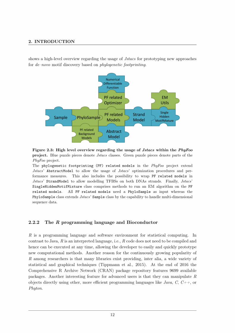
Jstacs is an open source Java library for the statistical analysis of biological sequences de-veloped by the groups Pattern Recognition and Bioinformatics at the Institute of ComputerScience of Martin Luther University Halle-Wittenberg and the Bioinformatics group of theJulius Kuehn Institute (Grau, Keilwagen, et al., 2012). Jstacs provides convenient andefficient classes for the representation of sequence data, many statistical models suitablefor the prediction of TFBSs in sequence data, ready to use numerical optimization proce-dures, and several performance measures. The design of Jstacs is a strictly object-orientedframework with a deep class hierarchy and there is a rich documentation. Hence, Jstacs iseasy-to-use, extensible, and customizable to a great extend.

In this thesis, my colleagues and I use Jstacs to implement prototypes of new approachesfor de–novo motif discovery based on phylogenetic footprinting (Sections 3.2.1-3.2.3 andSections 5.1-5.3). Specifically, we extend the class Sample from Jstacs by the capa-bility to handle multi-dimensional sequence data (e.g. alignments). We the resultingclass PhyloSample also provides convenient methods for the processing of phylogeneticdata. Further, we implement several Models related to phylogenetic footprinting extendingJstacs’ AbstractModel class. This allows us to use optimization procedures and perfor-mance measures available in Jstacs and thus facilitates development and decreases theprobability of implementation bugs. Finally, we extend Jstacs’ numerical optimizationprocedures by the capability to optimize parameters from phylogenetic trees and PFMs.We make our implementations available in the PhyFoo project on GitHub1. Figure 2.3

1https://github.com/mgledi/PhyFoo

11

Page 22

2. INTRODUCTION

shows a high-level overview regarding the usage of Jstacs for prototyping new approachesfor de–novo motif discovery based on phylogenetic footprinting.

Strand Model

PhyloSample PF related

Models Sample

AbstractModel

Numerical Differentiable

Function

PF related Optimizer

Single Hidden

MotifMixture

PF related Background

Models

EM Utils

Figure 2.3: High level overview regarding the usage of Jstacs within the PhyFooproject. Blue puzzle pieces denote Jstacs classes. Green puzzle pieces denote parts of thePhyFoo project.The phylogenetic footprinting (PF) related models in the PhyFoo project extendJstacs’ AbstractModel to allow the usage of Jstacs’ optimization procedures and per-formance measures. This also includes the possibility to wrap PF related models inJstacs’ StrandModel to allow modelling TFBSs on both DNAs strands. Finally, Jstacs’SingleHiddenMotifMixture class comprises methods to run an EM algorithm on the PFrelated models. All PF related models need a PhyloSample as input whereas thePhyloSample class extends Jstacs’ Sample class by the capability to handle multi-dimensionalsequence data.

2.2.2 The R programming language and Bioconductor

R is a programming language and software environment for statistical computing. Incontrast to Java, R is an interpreted language, i.e., R code does not need to be compiled andhence can be executed at any time, allowing the developer to easily and quickly prototypenew computational methods. Another reason for the continuously growing popularity ofR among researchers is that many libraries exist providing, inter alia, a wide variety ofstatistical and graphical techniques (Tippmann et al., 2015). At the end of 2016 theComprehensive R Archive Network (CRAN) package repository features 9699 availablepackages. Another interesting feature for advanced users is that they can manipulate Robjects directly using other, more efficient programming languages like Java, C, C++, orPhyton.

12

Page 23

2.2 Computer science background

R is extensively used in the field of bioinformatics and Bioconductor is an open developmentsoftware project that provides many high quality R packages regarding this field (R. C.Gentleman et al., 2004). Specifically, the Bioconductor project provides over 1000 powerfulstatistical and graphical packages for the analysis of genomic data. Popular examples arethe package genefilter for the filtering of genes from high–throughput data (Bourgon etal., 2010), the package GenomicAlignments for the handling of short genomic alignments(M. Lawrence et al., 2013), and the package seqLogo for the visualization of sequencemotifs (Bembom, n.d.). It also provides over 900 packages with annotation data for, e.g.,human, mouse, yeast, or rockcress (Huber et al., 2015). A popular example in this groupis the biomaRt package which integrates BioMart data resources (e.g. Ensembl) with dataanalysis software in Bioconductor (Durinck et al., 2005). Further, the Bioconductor projectcontains more than 300 packages providing extensive experimental data of any kind, e.g.,sequencing data or expression data.

I also want to mention the two projects Shiny1 and OpenCPU 2 that allow the integrationof R into a web-server and hence make it easy to publish and share work with otherresearchers.

Regarding this thesis, R is used to implement DiffLogo (Sections 3.3.1, 3.3.2 and 6.1).DiffLogo is available as R package in the Bioconductor software suite3 and via GitHub4.

2.2.3 Databases

Databases are used to store collections of data. The data are typically organized in astructured way enabling fast and purposeful access. There exist hundreds of differentdatabases that can be divided into two groups.

The first group, relational databases, comprises databases that are based on the relationalmodel of data (Codd, 1970). That means, that data is organized in tables consisting ofrows and columns, where each row can be identified with a unique key. Data in a relationaldatabase can be queried using structured query language (SQL). Relational databases areused when the structure of the data is well defined, i.e., rely on a schema, and when thedata is mainly accessed using complex queries with many relations. Examples for relationaldatabases are MySQL, DB2, or PostgreSQL. Regarding this thesis, MySQL is used for theimplementation of miRGen (Sections 3.1.1 and 4.1).

The second group, not only SQL (NoSQL) databases or non relational databases, areoften simpler designed than relational databases and typically lack tabular relations. The

1https://shiny.rstudio.com/2https://www.opencpu.org/3http://bioconductor.org/packages/release/bioc/html/DiffLogo.html4https://github.com/mgledi/DiffLogo

13

Page 24

2. INTRODUCTION

data stored in NoSQL databases can be unstructured, i.e., NoSQL databases are typicallyschema-free. Hence, these databases are typically faster, can store more data, have a higherscalability, and are easier to maintain. Examples for NoSQL databases are MongoDB,Cassandra, or BerkleyDB.

Sometimes, it is not sufficient to just choose a meaningful database or database manage-ment system for a certain data handling problem. In these cases a comprehensive storageconcept is needed. One example for such a storage concept is the Disk Repository withUpdate Management (DRUM ) concept which was initially proposed by Lee et al. to storebillions of URLs with meta-data using a single-server implementation (Lee et al., 2009).The central idea of the DRUM concept is to maintain fast sequential read and write accessfrom and to the underlying storage device by holding and preparing as much records aspossible in memory.

In context of this thesis, my colleagues and I propose a NoSQL database based on theDRUM concept for the management of large biological datasets on single desktop hardware(Sections 3.1.2 and 4.2).

2.3 Bioinformatics background

This section introduces the reader into the fields of bioinformatics touched by this thesisand its limitations. Specifically, this section includes a brief description of integration of bi-ological data (Section 2.3.1) and ChIP-seq data analysis (Section 2.3.2). The reader willalso be introduced to the idea of de–novo motif discovery based on phylogenetic footprinting(Section 2.3.3) and to the visualization of sequence motifs (Section 2.3.4).

2.3.1 Integration of biological data

With the continuously growing amount of biological data, the need to store, share, andorganize it also grows. The current NAR database issue comprises 62 articles describingnew biological databases and 112 articles describing updates on existing databases fore.g., storing ChIP-seq data (Daniel J Rigden et al., 2016). The online molecular biologydatabase collection therewith now comprises 1685 biological databases (Daniel J. Rigdenet al., 2016).

Biological databases can be divided into primary and secondary databases. Primarydatabases typically contain data of only one type. Their main purpose is completenessand up-to-dateness. Secondary databases often combine data from primary databases andtypically already analyze the data depending on the corresponding requirements.

14

Page 25

2.3 Bioinformatics background

My colleagues and I identified two limitations regarding biological databases. First, thereexists no database that provides comprehensive information about miRNA transcripts to-gether with their regulation by transcription factors, expression profiles, SNPs, and miRNAtargets. We address this problem in Sections 3.1.1 and 4.1. Second, there exists nodatabase that is capable of storing billions of position-specific DNA-related records, per-forming fast and resource saving requests, and running on a standard personal computer.We propose a database which fulfills these requirements and we present our idea in Sec-tions 3.1.2 and 4.2.

2.3.2 ChIP-seq data analysis

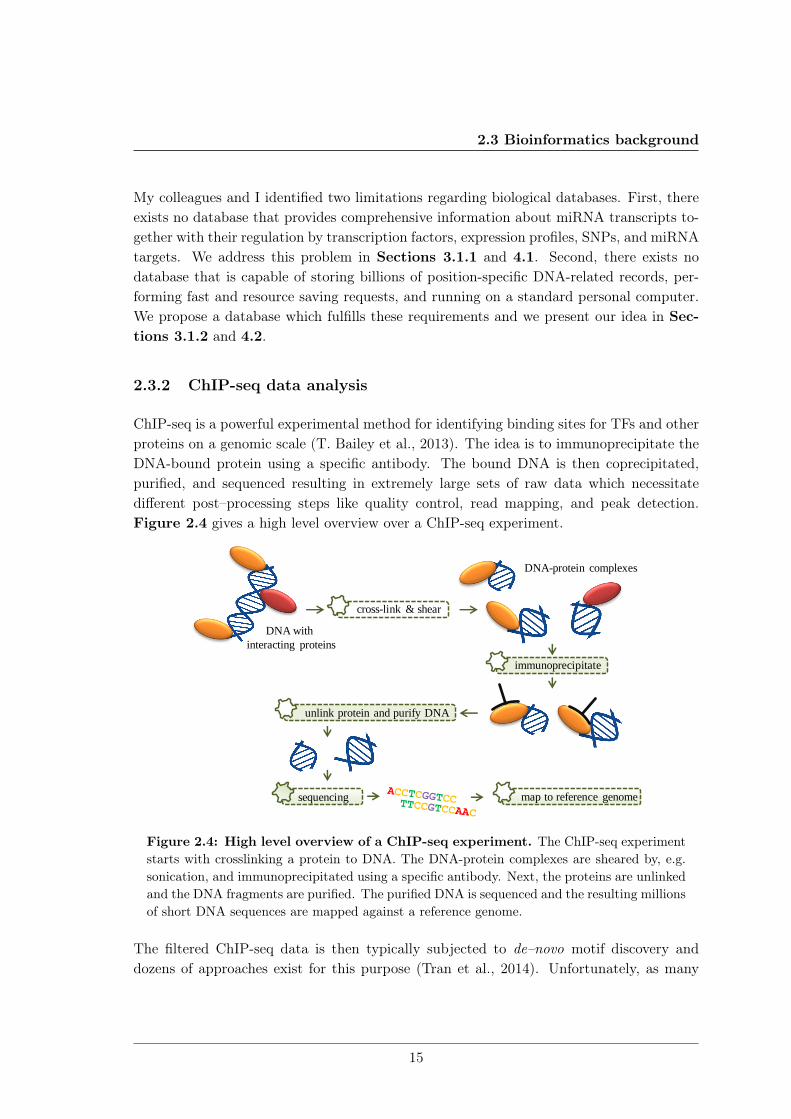
ChIP-seq is a powerful experimental method for identifying binding sites for TFs and otherproteins on a genomic scale (T. Bailey et al., 2013). The idea is to immunoprecipitate theDNA-bound protein using a specific antibody. The bound DNA is then coprecipitated,purified, and sequenced resulting in extremely large sets of raw data which necessitatedifferent post–processing steps like quality control, read mapping, and peak detection.Figure 2.4 gives a high level overview over a ChIP-seq experiment.

cross-link & shear

immunoprecipitate

unlink protein and purify DNA

sequencing

DNA with

interacting proteins

DNA-protein complexes

map to reference genome

Figure 2.4: High level overview of a ChIP-seq experiment. The ChIP-seq experimentstarts with crosslinking a protein to DNA. The DNA-protein complexes are sheared by, e.g.sonication, and immunoprecipitated using a specific antibody. Next, the proteins are unlinkedand the DNA fragments are purified. The purified DNA is sequenced and the resulting millionsof short DNA sequences are mapped against a reference genome.

The filtered ChIP-seq data is then typically subjected to de–novo motif discovery anddozens of approaches exist for this purpose (Tran et al., 2014). Unfortunately, as many

15

Page 26

2. INTRODUCTION

other techniques, motifs predicted by these computational approaches are distorted by thepresence of various biases, such as the ubiquitous binding-affinity bias (Håndstad et al.,2011; Ross et al., 2013; Timothy L. Bailey, Krajewski, et al., 2013). My colleagues and Ipropose an approach to estimate and diminish the BA bias in ChIP-seq data. We presentour idea in Sections 3.2.1 and 5.1.

2.3.3 De–novo motif discovery based on phylogenetic footprinting

The last decade has witnessed a spectacular development of sequencing technologies un-leashing new potentials in identifying TFBSs (D. S. Johnson et al., 2007; I. V. Kulakovskiyet al., 2010; Furey, 2012). Countless approaches exist for predicting TFBSs of known TFsand for de–novo motif discovery of TFBSs in sequence data. There are many meaningfulways to group these approaches. Tran et al. (Tran et al., 2014) grouped several mo-tif finding web tools by the way the sequence motif is modelled. The resulting groupsare Profiles, consensus sequences (Consensuses), Projections, Graph representations, Clus-tering of k-mers, and Tree-based data structures. Another way to distinguish differentapproaches could be by learning principle like generative learning principles and discrim-inative learning principles. A list with 36 different tools for motif discovery is availablein the supplement of the work of Zambelli et al. (2012). In this thesis, we divide ap-proaches for de–novo motif discovery into phylogenetic approaches and non-phylogeneticor single-species approaches.

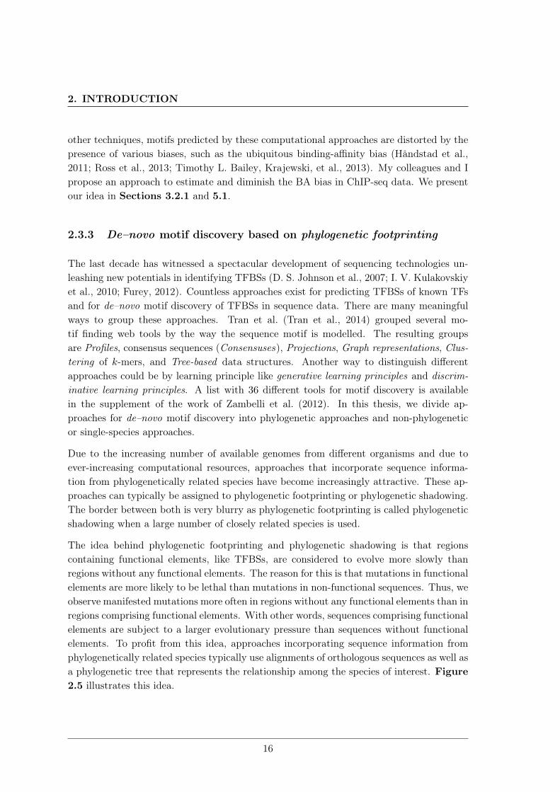
Due to the increasing number of available genomes from different organisms and due toever-increasing computational resources, approaches that incorporate sequence informa-tion from phylogenetically related species have become increasingly attractive. These ap-proaches can typically be assigned to phylogenetic footprinting or phylogenetic shadowing.The border between both is very blurry as phylogenetic footprinting is called phylogeneticshadowing when a large number of closely related species is used.

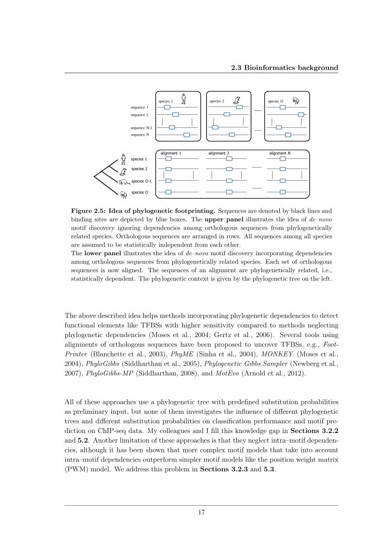
The idea behind phylogenetic footprinting and phylogenetic shadowing is that regionscontaining functional elements, like TFBSs, are considered to evolve more slowly thanregions without any functional elements. The reason for this is that mutations in functionalelements are more likely to be lethal than mutations in non-functional sequences. Thus, weobserve manifested mutations more often in regions without any functional elements than inregions comprising functional elements. With other words, sequences comprising functionalelements are subject to a larger evolutionary pressure than sequences without functionalelements. To profit from this idea, approaches incorporating sequence information fromphylogenetically related species typically use alignments of orthologous sequences as well asa phylogenetic tree that represents the relationship among the species of interest. Figure2.5 illustrates this idea.

16

Page 27

2.3 Bioinformatics background

sequence 1

species 1

sequence 2

sequence N-1

sequence N

species 2 species O

alignment 1 alignment N alignment 2

species 1

species 2

species O

species O-1

Figure 2.5: Idea of phylogenetic footprinting. Sequences are denoted by black lines andbinding sites are depicted by blue boxes. The upper panel illustrates the idea of de–novomotif discovery ignoring dependencies among orthologous sequences from phylogeneticallyrelated species. Orthologous sequences are arranged in rows. All sequences among all speciesare assumed to be statistically independent from each other.The lower panel illustrates the idea of de–novo motif discovery incorporating dependenciesamong orthologous sequences from phylogenetically related species. Each set of orthologoussequences is now aligned. The sequences of an alignment are phylogenetically related, i.e.,statistically dependent. The phylogenetic context is given by the phylogenetic tree on the left.

The above described idea helps methods incorporating phylogenetic dependencies to detectfunctional elements like TFBSs with higher sensitivity compared to methods neglectingphylogenetic dependencies (Moses et al., 2004; Gertz et al., 2006). Several tools usingalignments of orthologous sequences have been proposed to uncover TFBSs, e.g., Foot-Printer (Blanchette et al., 2003), PhyME (Sinha et al., 2004), MONKEY (Moses et al.,2004), PhyloGibbs (Siddharthan et al., 2005), Phylogenetic Gibbs Sampler (Newberg et al.,2007), PhyloGibbs-MP (Siddharthan, 2008), and MotEvo (Arnold et al., 2012).

All of these approaches use a phylogenetic tree with predefined substitution probabilitiesas preliminary input, but none of them investigates the influence of different phylogenetictrees and different substitution probabilities on classification performance and motif pre-diction on ChIP-seq data. My colleagues and I fill this knowledge gap in Sections 3.2.2and 5.2. Another limitation of these approaches is that they neglect intra–motif dependen-cies, although it has been shown that more complex motif models that take into accountintra–motif dependencies outperform simpler motif models like the position weight matrix(PWM) model. We address this problem in Sections 3.2.3 and 5.3.

17

Page 28

2. INTRODUCTION

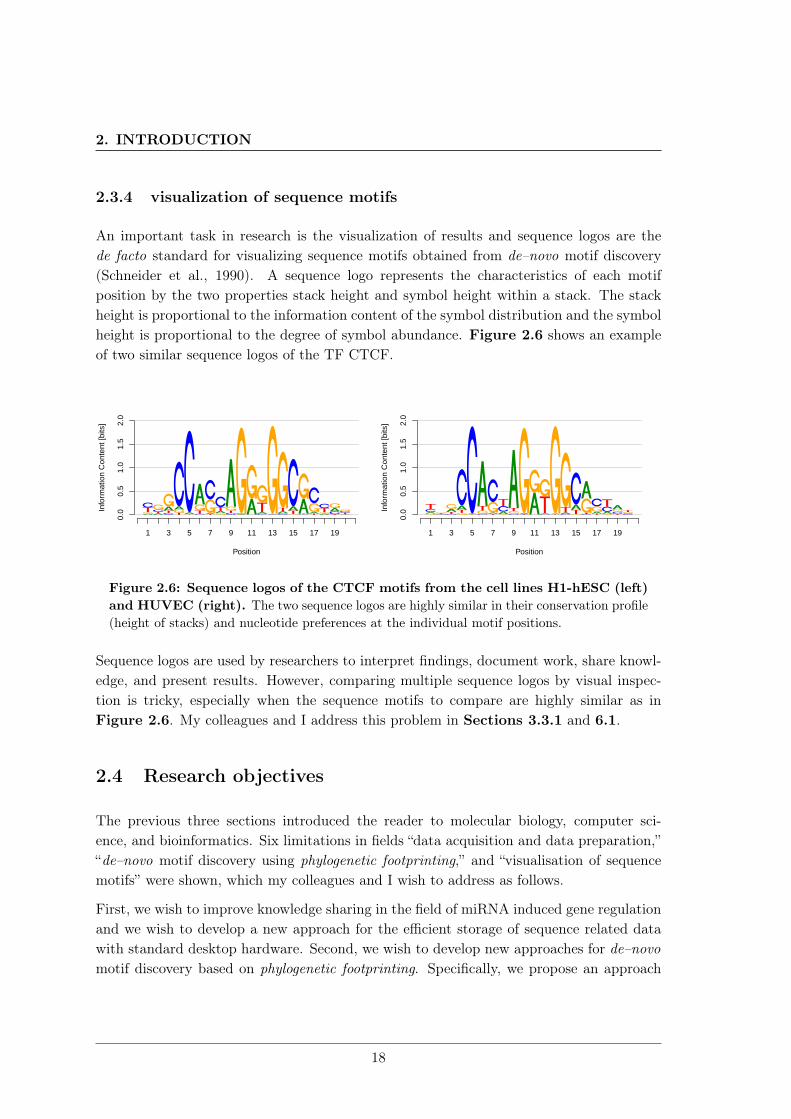
2.3.4 visualization of sequence motifs

An important task in research is the visualization of results and sequence logos are thede facto standard for visualizing sequence motifs obtained from de–novo motif discovery(Schneider et al., 1990). A sequence logo represents the characteristics of each motifposition by the two properties stack height and symbol height within a stack. The stackheight is proportional to the information content of the symbol distribution and the symbolheight is proportional to the degree of symbol abundance. Figure 2.6 shows an exampleof two similar sequence logos of the TF CTCF.

0.0

0.5

1.0

1.5

2.0

Position

Info

rmat

ion

Con

tent

[bits

]

1 3 5 7 9 11 13 15 17 19

0.0

0.5

1.0

1.5

2.0

Position

Info

rmat

ion

Con

tent

[bits

]

1 3 5 7 9 11 13 15 17 19

Figure 2.6: Sequence logos of the CTCF motifs from the cell lines H1-hESC (left)and HUVEC (right). The two sequence logos are highly similar in their conservation profile(height of stacks) and nucleotide preferences at the individual motif positions.

Sequence logos are used by researchers to interpret findings, document work, share knowl-edge, and present results. However, comparing multiple sequence logos by visual inspec-tion is tricky, especially when the sequence motifs to compare are highly similar as inFigure 2.6. My colleagues and I address this problem in Sections 3.3.1 and 6.1.

2.4 Research objectives

The previous three sections introduced the reader to molecular biology, computer sci-ence, and bioinformatics. Six limitations in fields “data acquisition and data preparation,”“de–novo motif discovery using phylogenetic footprinting,” and “visualisation of sequencemotifs” were shown, which my colleagues and I wish to address as follows.

First, we wish to improve knowledge sharing in the field of miRNA induced gene regulationand we wish to develop a new approach for the efficient storage of sequence related datawith standard desktop hardware. Second, we wish to develop new approaches for de–novomotif discovery based on phylogenetic footprinting. Specifically, we propose an approach

18

Page 29

2.4 Research objectives

based on phylogenetic footprinting to detect and correct the ubiquitous BA bias in ChIP-seqdata. Further, we systematically study the influence of phylogenetic trees with differentsubstitution probabilities on the classification performance of phylogenetic footprintingusing synthetic and real data. Finally, we extend phylogenetic footprinting by the capabilityof taking into account intra-motif dependencies. Third, we wish to improve the comparativevisualization of sequence motifs.

An important task in bioinformatics is the prediction of TFBSs in sequence data. Thistask typically starts with data acquisition and data preparation, e.g., sequence data areobtained from a ChIP-seq experiment. After transforming the data into an appropriateformat, de–novo motif discovery is performed and putative TFBSs are predicted. Finally,the results are visualized and compared to related work. With this thesis, I wish tocontribute to each of these three steps.

19

Page 30

2. INTRODUCTION

20

Page 31

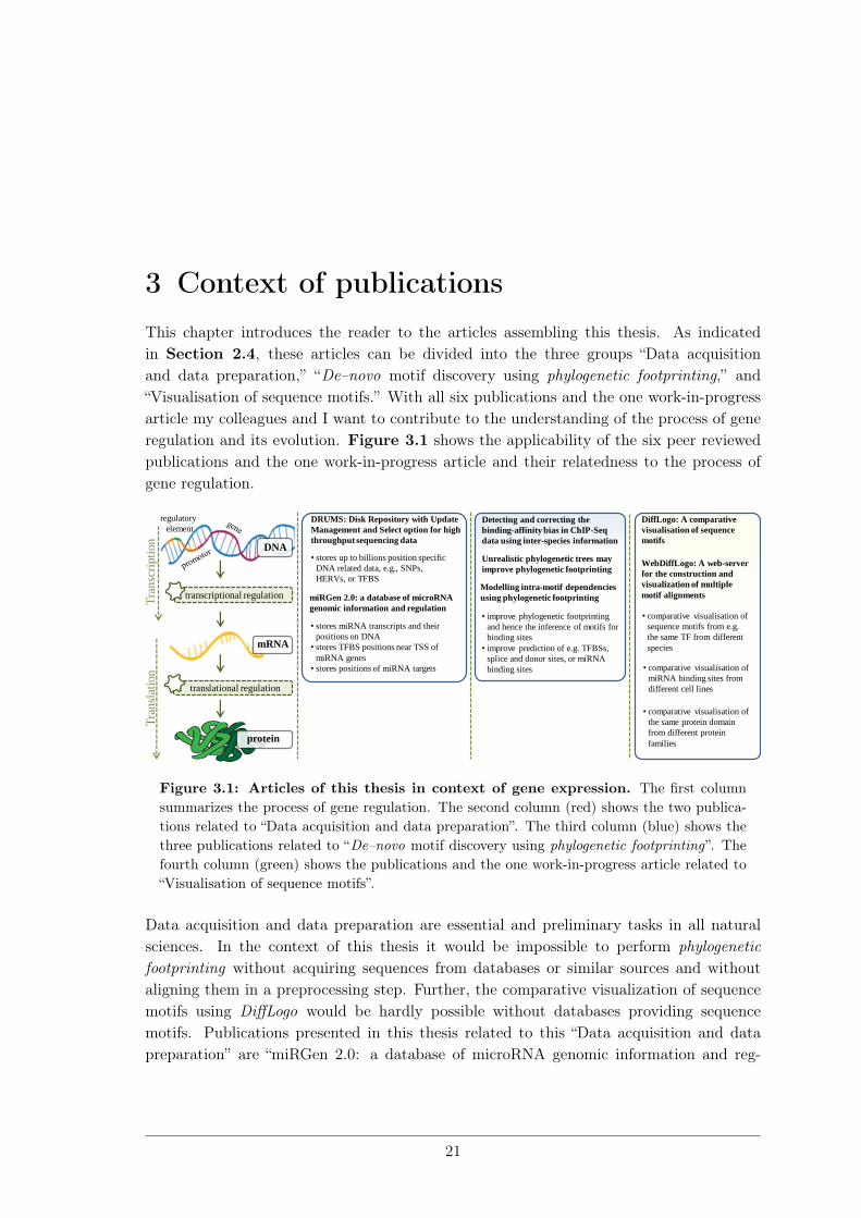
3 Context of publicationsThis chapter introduces the reader to the articles assembling this thesis. As indicatedin Section 2.4, these articles can be divided into the three groups “Data acquisitionand data preparation,” “De–novo motif discovery using phylogenetic footprinting,” and“Visualisation of sequence motifs.” With all six publications and the one work-in-progressarticle my colleagues and I want to contribute to the understanding of the process of generegulation and its evolution. Figure 3.1 shows the applicability of the six peer reviewedpublications and the one work-in-progress article and their relatedness to the process ofgene regulation.

Detecting and correcting the

binding-affinity bias in ChIP-Seq

data using inter-species information

Unrealistic phylogenetic trees may

improve phylogenetic footprinting

Modelling intra-motif dependencies

using phylogenetic footprinting

DiffLogo: A comparative

visualisation of sequence

motifs

regulatory

element

DNA

mRNA

protein

transcriptional regulation

Tra

nsc

ripti

on

T

ran

slat

ion

translational regulation

DRUMS: Disk Repository with Update

Management and Select option for high

throughput sequencing data

miRGen 2.0: a database of microRNA

genomic information and regulation • comparative visualisation of

sequence motifs from e.g.

the same TF from different

species

• comparative visualisation of

miRNA binding sites from

different cell lines

• comparative visualisation of

the same protein domain

from different protein

families

• improve phylogenetic footprinting

and hence the inference of motifs for

binding sites

• improve prediction of e.g. TFBSs,

splice and donor sites, or miRNA

binding sites

• stores miRNA transcripts and their

positions on DNA

• stores TFBS positions near TSS of

miRNA genes

• stores positions of miRNA targets

• stores up to billions position specific

DNA related data, e.g., SNPs,

HERVs, or TFBS

WebDiffLogo: A web-server

for the construction and

visualization of multiple

motif alignments

Figure 3.1: Articles of this thesis in context of gene expression. The first columnsummarizes the process of gene regulation. The second column (red) shows the two publica-tions related to “Data acquisition and data preparation”. The third column (blue) shows thethree publications related to “De–novo motif discovery using phylogenetic footprinting”. Thefourth column (green) shows the publications and the one work-in-progress article related to“Visualisation of sequence motifs”.

Data acquisition and data preparation are essential and preliminary tasks in all naturalsciences. In the context of this thesis it would be impossible to perform phylogeneticfootprinting without acquiring sequences from databases or similar sources and withoutaligning them in a preprocessing step. Further, the comparative visualization of sequencemotifs using DiffLogo would be hardly possible without databases providing sequencemotifs. Publications presented in this thesis related to this “Data acquisition and datapreparation” are “miRGen 2.0: a database of microRNA genomic information and reg-

21

Page 32

3. CONTEXT OF PUBLICATIONS

ulation” and “DRUMS: Disk Repository with Update Management and Select option forhigh throughput sequencing data”. Regarding the process of gene regulation, miRGen sup-ports researchers that are interested in miRNA regulation and miRNA function providingmiRNA transcripts with target genes, SNPs, TFBSs in near distance, and prominent lit-erature sources. Whereas DRUMS is applicable when dealing with hundred millions upto billions of DNA related information, like SNPs, TF binding site probabilities or humanendogenous retrovirus (HERV) occurrences in the human genome.

De–novo motif discovery is an essential task in bioinformatics and a preliminary for under-standing the process of gene regulation. Phylogenetic footprinting comprises approaches forde–novo motif discovery that take into account sequences of at least two phylogeneticallyrelated species. Publications presented in this thesis related to “De–novo motif discoveryusing phylogenetic footprinting” are “Detecting and correcting the binding-affinity bias inChIP-seq data using inter-species information”, “Unrealistic phylogenetic trees may improvephylogenetic footprinting”, and “Combining phylogenetic footprinting with motif modelsincorporating intra-motif dependencies”. All three proposed approaches may lead to animproved prediction of TFBSs and thus advance our understanding of transcriptional generegulation and its evolution.

The visualization of results is an essential task in all sciences and it is needed to interpretfindings, document work, share knowledge, and present results. Work related to “Visu-alisation of sequence motifs” in this thesis are the publication “DiffLogo: a comparativevisualization of sequence motifs” and the work-in-progress article “WebDiffLogo: A web-server for the construction and visualization of multiple motif alignments”.

The following subsections will introduce the reader into the publications and the one work-in-progress article comprising this work (Figure 3.1) and provide for each work a summaryon the addressed objectives, the used methods, and the results. The full articles arepresented in Chapters 4, 5, and 6.

3.1 Data acquisition and data preparation

The next two subsections provide a short summary of our publications “miRGen 2.0: adatabase of microRNA genomic information and regulation” and “DRUMS: Disk Reposi-tory with Update Management and Select option for high throughput sequencing data”.

22

Page 33

3.1 Data acquisition and data preparation

3.1.1 miRGen 2.0: a database of microRNA genomic information andregulation

The main objective of this work is to provide miRNA transcripts with related informationto researchers of diverse disciplines who are interested in the regulation and function ofmiRNAs. Therefore, we collect miRNA transcripts from prominent literature sources andenrich these transcripts with information about TFBSs near the transcription start sites(TSS), miRNA expression profiles, and SNPs in miRNA hairpins.

Methods

In this work, we collect 812 human miRNA coding transcripts and 386 mouse miRNAcoding transcripts from four literature sources. We identify for each miRNA primary tran-script putative TFBSs in the region 5 kb upstream and 1 kb downstream of the TSS usingMatchTM (Kel et al., 2003) and all vertebrate PWMs from Transfac 6.0 (Matys et al.,2003) minimizing the number of falsely predicted TFBSs. We provide for each predictedTFBS the matrix similarity score and the core similarity score calculated by MatchTM.We also identify miRNA expression profiles using the mammalian miRNA expression at-las (Ozsolak et al., 2008). We integrate data about SNPs located within the genomicpositions corresponding to miRNA hairpins and TFBSs from the UCSC table browser(Karolchik et al., 2009). All data of the miRGen repository are stored using the relationaldatabase management system MySQL. Figure 3.2 shows the relational schema of thedatabase.

Results, discussion, and conclusions

Over 800 miRNA transcripts with TFBSs near their TSS, miRNA expression profiles, andSNPs in the miRNA hairpins are stored in the miRGen repository and are accessible via auser-friendly interface that allows searches for miRNAs and/or TFs of interest. The inte-gration of the different information sources enables in-depth studies of miRNAs functionsand contributes to the understanding of post-transcriptional gene regulation. Currently,miRGen is cited by more than 100 articles, specifically in the field of cancer research (Juanet al., n.d.; H.-D. Huang, 2012; Mar-Aguilar et al., 2016) and hence contributes to cancerdiagnostics and therapeutics.

The TFBS annotations in miRGen from 2009 could be improved by using more sophisti-cated algorithms and motif models (instead of the PWM motif model) for the predictionof TFBSs. In addition, http://www.factorbook.org/ (J. Wang et al., 2012) meanwhileprovides extensive information for 167 TFs and their PWM representations for many exper-

23

Page 34

3. CONTEXT OF PUBLICATIONS

pathways through the application DIANA-mirPath (15).Figure 3 shows an overview of the interface and highlightslinks to external databases—UCSC genome browser (13),iHop (16), dbSNP (14), mirBase (11).

DISCUSSION

This version of miRGen is the first attempt to builda widely accessible and user-friendly database thatconnects TFs and miRNAs through putative and experi-mentally supported functional relationships. Theconnections identified in the database will further ourunderstanding of the TF-mediated regulation of miRNAgenes, and pave the way for the mapping of the interplaybetween TFs and miRNAs as regulatory molecules.The identification of SNPs on miRNA locations andtheir corresponding TFBSs, as well as the expressionprofiles of miRNAs can improve our insight into the

involvement of miRNAs in developmental processesand disease.

Deregulation of TF-mediated gene expression has beenshown to extensively affect protein coding genes, and leadto disease (17,18). MiRNA expression levels have alsobeen shown to change significantly in different diseasestates (19,20). The availability of both these resourcesin the same database will allow researchers to identifyregulatory elements, such as TFs that may affect theexpression of miRNAs. For this reason, we believemiRGen 2.0 will be an important resource for researchersof diverse disciplines interested in miRNA regulation andfunction.

AVAILABILITY

The miRGen database will be continuously maintainedand freely available at http://www.microrna.gr/mirgen/.

Figure 2. The miRGen database schema. TFs (top right) bind through TF binding sites to miRNA genes. miRNA genes (top) contain miRNAhairpins that signify the genomic location of the mature miRNA-miRNA* duplex. miRNA hairpins are processed into mature miRNAs. Usually,one miRNA hairpin produces two mature miRNAs, but a mature miRNA can be produced by more than one hairpin in different genomic locations.Both TFBSs and miRNA hairpins are genomic features that can contain SNPs. Mature miRNAs are associated with their expression levels indifferent tissues and cell types.

D140 Nucleic Acids Research, 2010, Vol. 38, Database issue

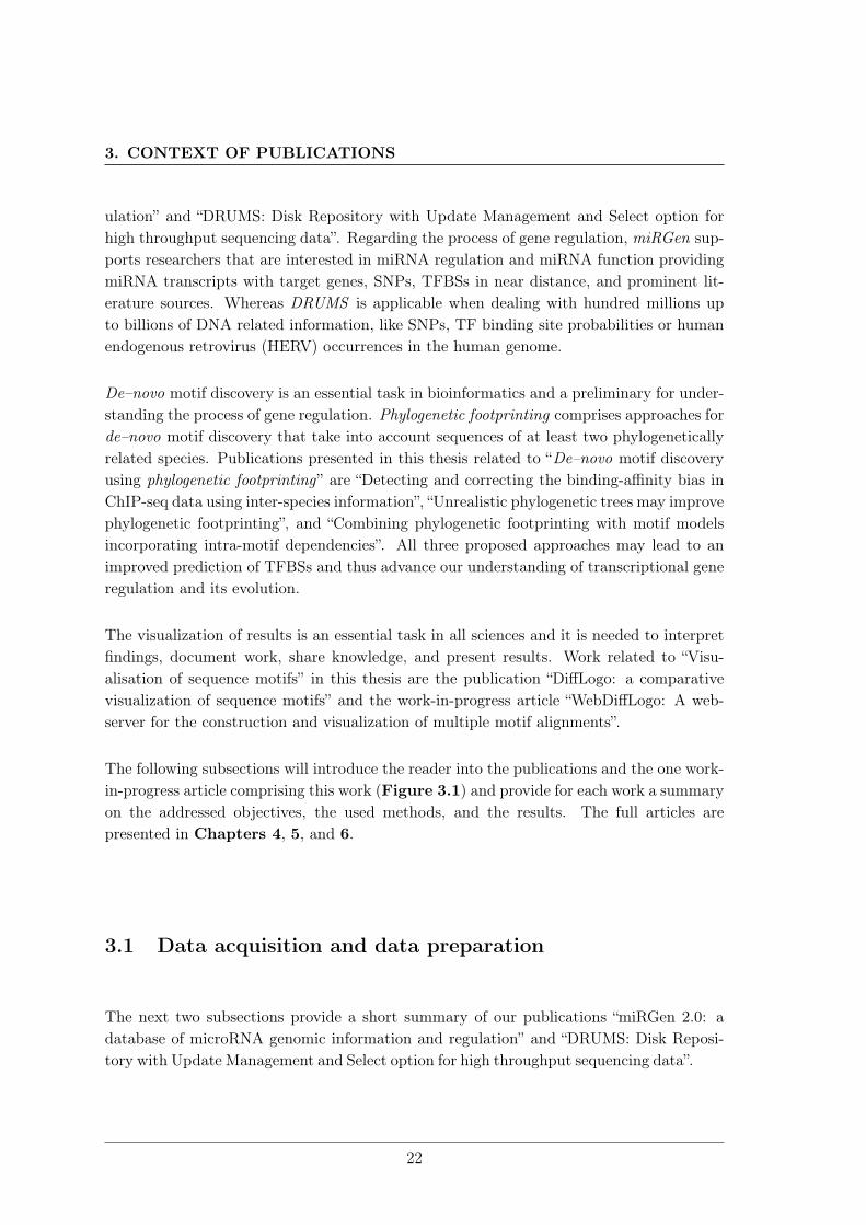
Figure 3.2: The miRGen database schema. TFs (top left) activate miRNA genes(top center) by binding to TFBSs (middle left). miRNA genes (top center) contain miRNAhairpins (middle right) that signify the genomic location of the mature miRNA-miRNA*duplex. miRNA hairpins are processed into mature miRNAs. Typically, one miRNA hairpinproduces two mature miRNAs, but a mature miRNA can be produced by more than onehairpin from different miRNA genes. Both TFBSs and miRNA hairpins are genomic featuresthat can contain SNPs. Mature miRNAs are associated with expression levels in varioustissues and cell types.

24

Page 35

3.1 Data acquisition and data preparation

iments from the ENCODE project (E. P. Consortium et al., 2004). Since many researchersuse data from the ENCODE project for their research it would be of advantage if miRGenwould use PWMs predicted on the very same data.

This work refers to version 2.0 of miRGen. The current version of miRGen is 3.0. miRGenis freely available at http://www.microrna.gr/mirgen/.

3.1.2 DRUMS: Disk Repository with Update Management and Selectoption for high throughput sequencing data

An important task of bioinformatics in the scope of computational biology projects is theefficient and well-organized data management. In fact often neglected, this issue becomesessential when dealing with many data sets that consist of millions or even billions ofrecords. In addition, researchers from biology and biochemistry prefer to keep and analyzethese data sets on a standard desktop machine for reasons of data privacy, limited computerskills, and convenience. Noble, 2009 describes how to organize data in computationalbiology projects and Wilson et al., 2014 describes best practices for scientific computing.In this work we tackle the problem of handling large data sets on a single standard desktopmachine.

One kind of data extensively used in bioinformatics is position specific data related toDNA sequences. Examples are SNPs (Single Nucleotide Polymorphism 2012), transcriptionfactor binding affinities, and probabilities (M. Bulyk, 2003; Nguyen et al., 2009), RNAseqdata (Z. Wang et al., 2009; Malone et al., 2011), and mapping data from BLAST (M.Johnson et al., 2008). These data are essential for the understanding of biological andbiochemical processes. We generalize this kind of data by the term position-specific DNArelated data (psDrd).

Due to the rapid development of sequencing technologies and the ever-increasing number oftools and algorithms for analysing, manipulating, and combining psDrd, the data volumeis growing exponentially. Thus, requesting data becomes challenging and expensive and isoften tackled using specialised and/or distributed hardware. The objective of this work isthe development of a data repository that is capable of storing billions of records of psDrd,performing fast and resource saving requests, and running on a single standard desktophardware.

Methods

psDrd records have the following three characteristics that are important for finding ordeveloping a suitable data repository. First, a psDrd record is representable by a key-value

25

Page 36

3. CONTEXT OF PUBLICATIONS

pair, consisting of a unique key that defines a position on a sequence and a value thatis associated to this sequence position. Second, all psDrd records of the same kind arestorable using the same amount of memory. Third, researchers who work with psDrd areusually interested in all records near a certain sequence locus and the exact position of thislocus is typically unknown.

By literature research we found the DRUM concept which was designed to store billionsof URLs with meta data when crawling the world wide web (Lee et al., 2009). DRUMis already capable of storing large collections of key-value pairs by supporting fast bulkinserts without generating duplicate entries. Unfortunately, DRUM was not designed torequest data in an efficient manner. We extended the DRUM concept by the capability ofrequesting a single record by key or a set of records in an interval between two keys. Wedeveloped the open-source Java library DRUMS meeting our requirements.

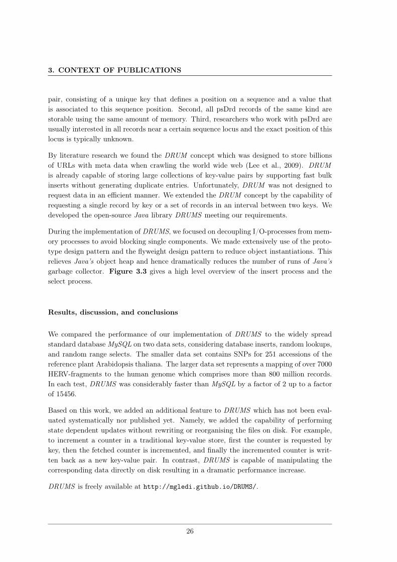
During the implementation of DRUMS, we focused on decoupling I/O-processes from mem-ory processes to avoid blocking single components. We made extensively use of the proto-type design pattern and the flyweight design pattern to reduce object instantiations. Thisrelieves Java’s object heap and hence dramatically reduces the number of runs of Java’sgarbage collector. Figure 3.3 gives a high level overview of the insert process and theselect process.

Results, discussion, and conclusions

We compared the performance of our implementation of DRUMS to the widely spreadstandard database MySQL on two data sets, considering database inserts, random lookups,and random range selects. The smaller data set contains SNPs for 251 accessions of thereference plant Arabidopsis thaliana. The larger data set represents a mapping of over 7000HERV-fragments to the human genome which comprises more than 800 million records.In each test, DRUMS was considerably faster than MySQL by a factor of 2 up to a factorof 15456.

Based on this work, we added an additional feature to DRUMS which has not been eval-uated systematically nor published yet. Namely, we added the capability of performingstate dependent updates without rewriting or reorganising the files on disk. For example,to increment a counter in a traditional key-value store, first the counter is requested bykey, then the fetched counter is incremented, and finally the incremented counter is writ-ten back as a new key-value pair. In contrast, DRUMS is capable of manipulating thecorresponding data directly on disk resulting in a dramatic performance increase.

DRUMS is freely available at http://mgledi.github.io/DRUMS/.

26

Page 37

3.2 Predicting transcription factor binding sites using phylogeneticfootprinting

incomimg data<key, value> tuples

RAM disk

<key, value> buffer 1

<key, value> buffer 2

<key, value> buffer k

...

bucket 1

bucket 2

bucket k

...

Syn

chro

nizi

ng P

roce

ss

requesting records between key1 and key2

RAM disk

bucket 1

bucket 2

bucket k

Mapping and Indices

determine bucket with key1 and its position in this bucket

Read Buffersequentially read from determined position until key2 is reached and filter affected records into buffer

...

Figure 3.3: High level overview of the insert (left) and the select process (right)in DRUMS.Insert process (left): Key-value pairs are sent to DRUMS. The incoming records are dis-tributed between k buffers (memory buckets), based on their key. If a bucket Bi exceeds apredefined size or overall memory limitations are reached, a synchronisation process is instan-tiated.Select process (right): A request is sent to DRUMS, typically providing a lower and anupper key. The following four steps are performed to get the requested records. 1) The bucketof interest is determined. 2) The correct chunk of the first requested record is identified, usinga sparse index. 3) The position of the requested key-value pair is determined. 4) A sequentialread is performed until the requested range is completely processed.

3.2 Predicting transcription factor binding sites using phylo-genetic footprinting

The next three subsections provide a short summary of our publications “Detecting andcorrecting the binding-affinity bias in ChIP-seq data using inter-species information”, “Un-realistic phylogenetic trees may improve phylogenetic footprinting”, and “Combining phy-logenetic footprinting with motif models incorporating intra-motif dependencies”.

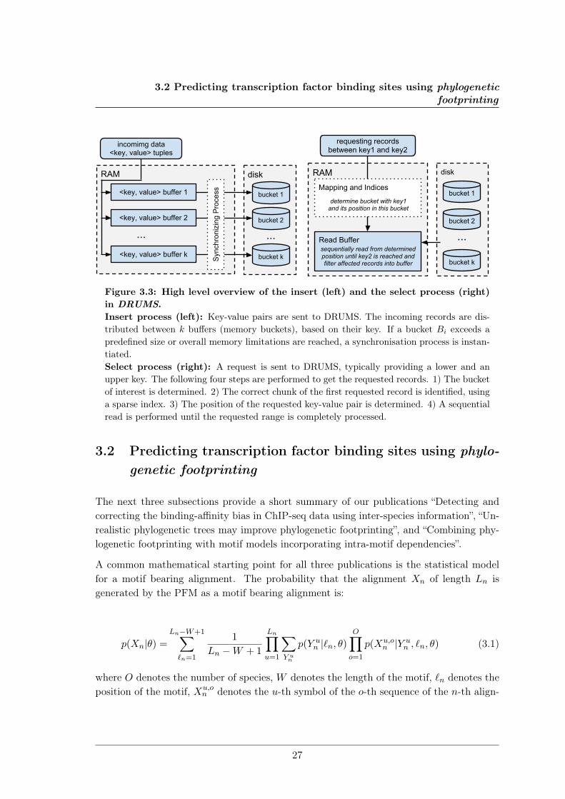
A common mathematical starting point for all three publications is the statistical modelfor a motif bearing alignment. The probability that the alignment Xn of length Ln isgenerated by the PFM as a motif bearing alignment is:

p(Xn|θ) =Ln−W+1∑`n=1

1

Ln −W + 1

Ln∏u=1

∑Y un

p(Y un |`n, θ)

O∏o=1

p(Xu,on |Y u

n , `n, θ) (3.1)

where O denotes the number of species, W denotes the length of the motif, `n denotes theposition of the motif, Xu,o

n denotes the u-th symbol of the o-th sequence of the n-th align-

27

Page 38

3. CONTEXT OF PUBLICATIONS

ment, and Y un denotes the u-th symbol in the ancestral sequence. θ denotes the set of model

parameters, namely the topology of the phylogenetic tree, the substitution probabilities,and the evolutionary model with its stationary probabilities for the flanking regions as wellas for the binding site regions. I refer this formula in the following subsections.

3.2.1 Detecting and correcting the binding-affinity bias in ChIP-Seqdata using inter-species information

The computational investigation of genomic regions containing TFBSs is a prerequisite forelucidating the process of gene regulation. ChIP-seq has become the major technology touncover genomic regions containing TFBSs and countless approaches exist for predictingmotifs from these genomic regions. It is known that ChIP-seq data and similar experimentaldata is contaminated with false positive genomic regions and there is evidence that there isan enrichment with high-affinity binding sites. Both factors potentially distort the resultsof de novo motif prediction which would affect all downstream analyses (Ross et al., 2013;Park et al., 2013; Teytelman et al., 2013; Elliott et al., 2015).

The contamination with false positive genomic regions leads to the contamination bias (Tim-othy L. Bailey, Krajewski, et al., 2013) and thus to the prediction of artificially softenedmotifs, whereas the enrichment of sequences with high-affinity binding sites leads to thebinding-affinity bias (Håndstad et al., 2011) and thus to the prediction of artificially sharp-ened motifs. Most existing approaches for de novo motif prediction are capable of detectingand correcting the contamination bias and it has been shown that this increases the qual-ity of motif prediction considerably (Timothy L. Bailey and Elkan, 1995; Wilbanks et al.,2010; Gomes et al., 2014).

The main objective of this work is to detect and correct the binding affinity bias andto improve phylogenetic footprinting by extending a traditional PFM that already takesinto account the contamination bias by the capability to also take into account the BAbias.

Methods

To our knowledge, it is impossible to detect the BA bias based on sequence data fromonly one species, but detecting the BA bias appears to be possible using sequences fromphylogenetically related species. The key idea is that mutations decrease the effect ofBA bias in phylogenetically related species. Hence, the direct effect of the BA bias inthe reference species is stronger than the indirect effect of the BA bias in phylogeneticallyrelated species. Under this assumption the information content of the predicted motif in thereference species should be higher than the information content of the predicted motifs in

28

Page 39

3.2 Predicting transcription factor binding sites using phylogeneticfootprinting

phylogenetically related species. More specifically, the information content of the predictedmotifs in the phylogenetically related species should decrease with the phylogenetic distancefrom the reference species. The detailed idea and a toy example can be found in the section"Using sequence information of phylogenetically related species to detect the binding-affinity bias" of the corresponding article (Nettling et al., 2016).

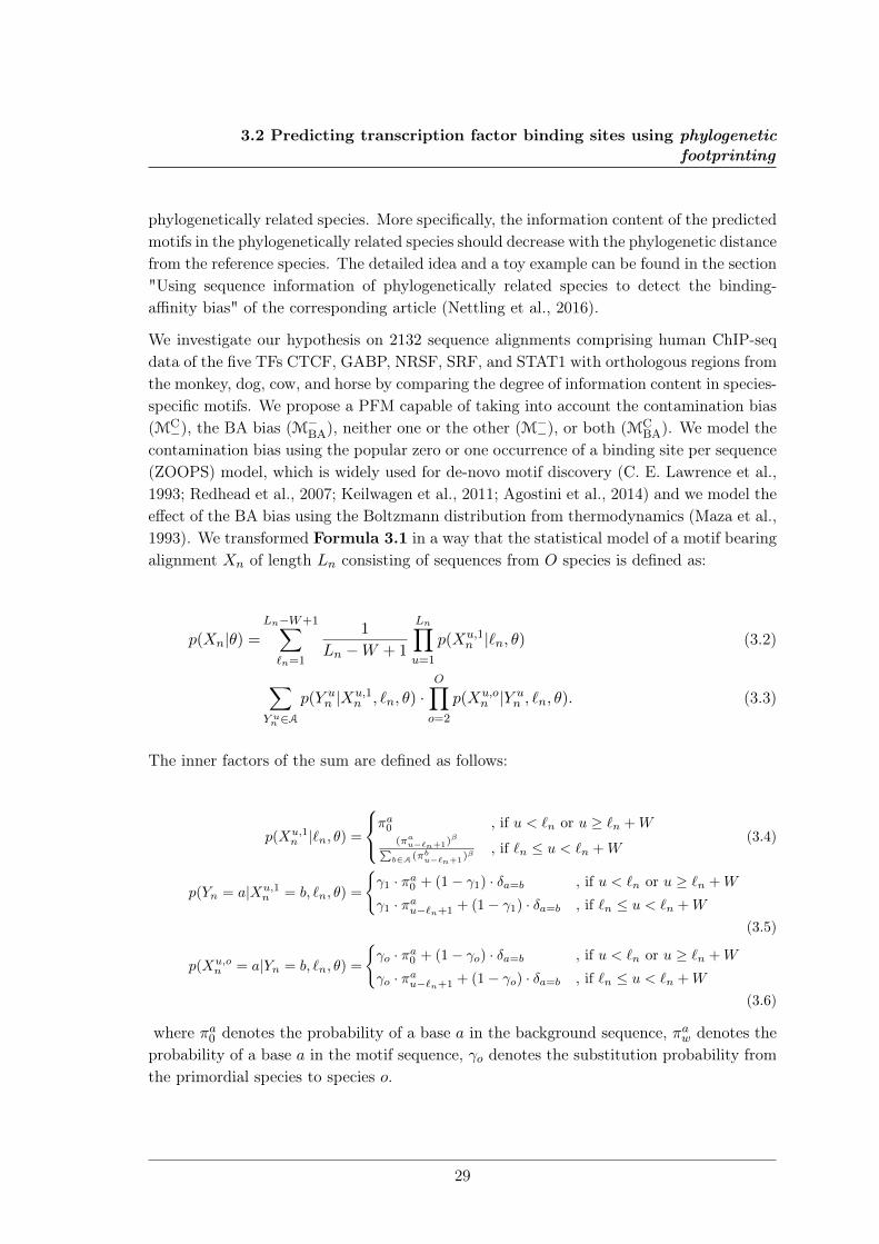
We investigate our hypothesis on 2132 sequence alignments comprising human ChIP-seqdata of the five TFs CTCF, GABP, NRSF, SRF, and STAT1 with orthologous regions fromthe monkey, dog, cow, and horse by comparing the degree of information content in species-specific motifs. We propose a PFM capable of taking into account the contamination bias(MC−), the BA bias (M−BA), neither one or the other (M−−), or both (MC

BA). We model thecontamination bias using the popular zero or one occurrence of a binding site per sequence(ZOOPS) model, which is widely used for de-novo motif discovery (C. E. Lawrence et al.,1993; Redhead et al., 2007; Keilwagen et al., 2011; Agostini et al., 2014) and we model theeffect of the BA bias using the Boltzmann distribution from thermodynamics (Maza et al.,1993). We transformed Formula 3.1 in a way that the statistical model of a motif bearingalignment Xn of length Ln consisting of sequences from O species is defined as:

p(Xn|θ) =Ln−W+1∑`n=1

1

Ln −W + 1

Ln∏u=1

p(Xu,1n |`n, θ) (3.2)

∑Y un ∈A

p(Y un |Xu,1

n , `n, θ) ·O∏o=2

p(Xu,on |Y u

n , `n, θ). (3.3)

The inner factors of the sum are defined as follows:

p(Xu,1n |`n, θ) =

πa0 , if u < `n or u ≥ `n +W(πau−`n+1)

β∑b∈A(πbu−`n+1)

β , if `n ≤ u < `n +W(3.4)

p(Yn = a|Xu,1n = b, `n, θ) =

{γ1 · πa0 + (1− γ1) · δa=b , if u < `n or u ≥ `n +W

γ1 · πau−`n+1 + (1− γ1) · δa=b , if `n ≤ u < `n +W

(3.5)

p(Xu,on = a|Yn = b, `n, θ) =

{γo · πa0 + (1− γo) · δa=b , if u < `n or u ≥ `n +W

γo · πau−`n+1 + (1− γo) · δa=b , if `n ≤ u < `n +W

(3.6)

where πa0 denotes the probability of a base a in the background sequence, πaw denotes theprobability of a base a in the motif sequence, γo denotes the substitution probability fromthe primordial species to species o.

29

Page 40

3. CONTEXT OF PUBLICATIONS

β denotes the inverse temperature from the Boltzmann distribution and quantifies thedegree of the BA bias in the reference species. We assume that a TF binds the bindingsite B with a probability proportional to p(B|π)β−1. As B occurs in vivo with probabilityp(B|π), it occurs in the set of immunoprecipitated sequences with a probability propor-tional to p(B|π) · p(B|π)β−1 = p(B|π)β . A value for β greater than one indicates that theChIP-seq data set is affected by the binding-affinity bias, i.e., high-affinity binding sitesare over-represented.

In Supplementary Section 1 of the corresponding article and in Section 7.1.1 of thisthesis, the reader can find a detailed definition of the probabilistic model that is capableof taking into account both the contamination bias and the BA bias. In the correspondingarticle, we describe the PFM that is capable of taking into account the BA bias from theperspective of the data generating process.

We measure the classification performance of the four models M−−, M−BA, M

C−, and MC

BA

using 100 fold stratified repeated random sub-sampling validation. We calculate the in-formation contents of the motifs predicted by the models taking into account the BAbias and the models neglecting the BA bias. We use DiffLogo to investigate differencesin sequence motifs predicted by M−BA and MC

BA and the traditional motifs predicted byM−− and MC

−.

Results, discussion, and conclusions

We found in case of all five TFs that the information contents of the human motifs aresignificantly higher than the information contents of the motifs from the monkey, dog,cow, and horse. We also found that the correction of the BA bias is possible using theproposed PFM leading to a more accurate inference of sequence motifs and to a moreprecise prediction of TFBSs. Interestingly, we found that the enrichment of ChIP-seqdata with high-affinity binding sites causes a distortion of DNA binding motifs that iseven stronger than the distortion caused by the contamination bias. The comparison ofnovel and traditional motifs showed small but noteworthy differences, suggesting that therefinement of traditional motifs from literature and databases might lead to the inferenceof novel binding sites, cis-regulatory modules, and gene-regulatory networks and may thusadvance our attempt of understanding transcriptional gene regulation as a whole.

3.2.2 Unrealistic phylogenetic trees may improve phylogenetic footprint-ing

Two prerequisites for most phylogenetic footprinting algorithms are multiple sequence align-ments (MSAs) of the DNA regions to analyse and phylogenetic trees, including substitution

30

Page 41

3.2 Predicting transcription factor binding sites using phylogeneticfootprinting

probabilities attached to the branches. These phylogenetic trees are used to quantify theevolution of functional elements and their flanking DNA in the input MSAs. Hence, thechoice of the phylogenetic trees and the substitution probabilities has a strong influenceon the performance of phylogenetic footprinting and hence on the prediction of TFBSs (Kcet al., 2011). Typically, the phylogenetic trees used by nature to evolve the DNA regions ofinterest have been lost and are unknown. Estimating appropriate phylogenetic trees withappropriate substitution probabilities is hardly possible (Blanchette et al., 2003), so thatthe needed information is often simply taken from literature or guessed.

There are many articles that state that phylogenetic footprinting improves motif predictionbut none of them investigates the influence of different phylogenetic trees on classificationperformance and motif prediction on non-synthetic data (Moses et al., 2004; Gertz et al.,2006; Clark et al., 2007; Hardison et al., 2012). Thus, the main objective of this workis to study systematically the influence of the phylogenetic trees on the performance ofphylogenetic footprinting.

Methods

To systematically investigate the influence of phylogenetic trees on the performance of phy-logenetic footprinting we made the following simplification. The PFM uses a star topologyinstead of a more complex phylogenetic tree with all branches having the same length, i.e.,the substitution probability γ is the same for all species. With this simplification it is nowpossible to investigate the performance of a PFM as function of the substitution proba-bility γ, where small γ encode closely phylogenetic relations and large γ encode looselyphylogenetic relations. The statistical model of a motif bearing alignment looks differentto Formula 3.1 but is the same. We extracted the parameter γ from the set of parameterset θ. The probability that the alignment Xn of length Ln consisting of sequences from O

observed species can be calculated as follows:

p(Xn|γ, θ) =Ln−W+1∑`n=1

1

Ln −W + 1

Ln∏u=1

∑Y un

p(Y un |`n, γ, θ)

O∏o=1

p(Xu,on |Y u

n , `n, γ, θ) (3.7)

The inner factors are defined as follows:

p(Y un |`n, γ, θ) =

{πa0 if u < `n or u ≥ `n +W

πau−`n+1 if `n ≤ u < `n +W(3.8)

p(Xu,kn |Y un , `n, γ, θ) =

{γ × πa0 + (1− γ)δa=b if u < `n or u ≥ `n +W

γ × πau−`n+1 + (1− γ)δa=b if `n ≤ u < `n +W(3.9)

31

Page 42

3. CONTEXT OF PUBLICATIONS

where πa0 denotes the probability of a base a in the background sequence, πaw denotes theprobability of a base a in the motif sequence, γk denotes the substitution probability fromthe primordial species to species k. The complete statistical model and all parameters areexplained in Methods 1 of the corresponding article.

We investigate the classification performance and the likelihood of the PFM for γ =

{0.05, 0.1, . . . , 1.0} on human ChIP-seq data of the five TFs CTCF, GABP, NRSF, SRF,and STAT1 enriched with orthologous regions from the monkey, dog, cow, and horse aswell as on synthetic data generated using a PFM with γ = 0.2. We further compare theclassification performance of the three PFMs using a tree from literature (Arnold et al.,2012) (Mtree

lit ), a star topology with the maximum likelihood estimated γ (MstarML ), and a

star topology with γ = 1 (Mstarγ=1.0).

Results, discussion, and conclusions

When studying the likelihood, we found that on synthetic data the best likelihood isachieved when using the same phylogenetic tree for learning as for data generation. Wealso observed that on organic data the best likelihood is achieved when using realisticphylogenetic trees indicating that we are capable of identifying reasonable substitutionprobabilities for synthetic and for real data using the maximum-likelihood principle.

When investigating the classification performance, we found that on synthetic data the bestclassification performance is achieved when using the same phylogenetic tree for learningas for data generation. In contrast, we found that on organic data unrealistic phylogenetictrees often lead to more accurate predictions of transcription factor binding sites than re-alistic phylogenetic trees. We also observed that Mstar

γ=1.0 significantly outperforms MstarML

and Mtreelit . With other words, choosing unrealistic model assumptions with phylogenetic

footprinting – namely using a star topology with unrealistic large substitution probabili-ties – may yield higher classification performances than using realistic phylogenetic treeswith more realistic substitution probabilities.

Although we have no concrete explanation for this observation, we speculate that evolution-ary effects like heterogeneous and heterotachious substitution probabilities among differentDNA positions are violating model assumptions like the assumption of time reversibility.Further, these effects might already have lead to the construction of incorrect or at leastpartially erroneous MSAs. PFMs using a star topology with substitution probabilities ofγ = 1 seem to be more robust toward these effects than PFMs using realistic phyloge-netic trees with realistic substitution probabilities. Hence, we need to give the strange butpractical recommendation to use PFMs based on these unrealistic model assumptions untilthere are more appropriate PFMs that take into account heterogeneity and heterotachy aswell as putative misalignments in the input MSAs.

32

Page 43

3.2 Predicting transcription factor binding sites using phylogeneticfootprinting

3.2.3 Combining phylogenetic footprinting with motif models incorpo-rating intra-motif dependencies

As stated repeatedly in this work, de-novo motif discovery is a challenging task in bioin-formatics and many different approaches exist for solving this task. These approaches canbe divided in two groups.

The first group comprises approaches using sequences of only one species, which we referto as one-species approaches. Within this group, a variety of statistical models are used forthe binding of TFs to their TFBSs, ranging from the simple PWM model, neglecting intra-motif dependencies, to more complex models, taking into-account intra-motif dependencies(Grau, Posch, et al., 2013; I. Kulakovskiy et al., 2013; Ma et al., 2014; Alipanahi et al.,2015; Siebert et al., 2016).

The second group comprises approaches using sequences of at least two phylogenetic relatedspecies, which is known as phylogenetic footprinting. Within this group, statistical modelsare used that are capable of modeling the binding of TFs to their TFBSs and their evolutionsimultaneously (Blanchette et al., 2003; Sinha et al., 2004; Moses et al., 2004; Siddharthanet al., 2005; Neph et al., 2006; Newberg et al., 2007; Siddharthan, 2008; Arnold et al.,2012).

It has been shown that more complex motif models taking into account intra-motif depen-dencies outperform simpler motif models like the PWM model and that models that takeinto account phylogenetic dependencies also outperform the PWM model (M. L. Bulyket al., 2002; Salama et al., 2010; Eggeling et al., 2015). One-species approaches neglectphylogenetic information, whereas phylogenetic footprinting, which incorporates this infor-mation, neglects intra-motif dependencies.

The main objective of this work is to improve phylogenetic footprinting by taking into ac-count base dependencies, i.e., developing an approach for de-novo motif discovery that takesinto account both phylogenetic dependencies and base dependencies simultaneously.

Methods

We extend a PFMmodel based on the Felsenstein evolutionary model (Felsenstein, 1981) bythe capability of taking into account base dependencies resulting in a model that is capableof taking into account base dependencies and phylogenetic dependencies simultaneously.We use Formula 3.1 as starting point and split up the product

∏Lnu=1 that takes into

account the whole alignment into three products, namely the region left of the motif, the

33

Page 44

3. CONTEXT OF PUBLICATIONS

motif region, and the region right of the motif. The statistical model of a motif bearingalignment Xn of length Ln consisting of sequences from O species is defined as:

p(Xn, θ) =

Ln−W+1∑`n=1

1

Ln −W + 1

O∏o=1

p(Xi(`n),on |`n, θ) · p(Xm(`n),o

n |`n, θ) · p(Xe(`n),on |`n, θ) (3.10)

The inner factors are defined as follows:

p(Xi(`n),on |`n, θ) =

∏u∈{1,...,`n−1}

πa,ζ0 (left flanking region) (3.11)

p(Xm(`n),on |`n, θ) =

∏u∈{`n,...,`n+W−1}

πa,ζu−`n+1 (motif region) (3.12)

p(Xe(`n),on |`n, θ) =

∏u∈{`n+W,...,Ln}

πa,ζ0 (right flanking region) (3.13)

where the probability of a base a in the background sequence provided that its predecessorsare in joint state ζ is given by the parameter πa,ζ0 and the probability of a base a in themotif sequence provided that its predecessors are in joint state ζ is given by the parameterπa,ζw . The complete statistical model and all parameters are explained in Methods 2 ofthe corresponding article.

We study the proposed PFMs on datasets based on ChIP-seq data of 35 TFs. First, wemeasure the degree of intra-motif dependencies captured by the proposed PFMs by com-puting the position–wise mutual information (mutual information). We call the resultingvector of mutual information values mutual information profile. For each of the 35 TFs,we compute the mutual information profiles of orders 1 and 2 from the motifs obtained bythe PFMs of order 2. Moreover, we study for each TF the similarity of the species–specificmotifs using DiffLogoand the similarity of the species–specific mutual information profilesusing statistical tests.

Second, we study the classification performance of the PFMs of orders 0, 1, and 2 using25–fold stratified repeated random sub-sampling validation. We calculate and show foreach TF the relative increase of the PFMs of orders 1 and 2 relative to the PFM oforder 0 Moreover, we compare the classification performance of phylogenetic footprintingand one-species approaches when neglecting and taking into account base dependencies oforder 2.

34

Page 45

3.3 Visualization of sequence motifs

Results, discussion, and conclusions

First, we found for the studied TFs statistically significant intra-motif dependencies be-tween neighboring bases at all positions and we found even stronger intra-motif depen-dencies between dimers and their neighboring bases at all positions. We excluded thepossibility that the captured intra-motif dependencies are an artifact resulting from a mix-ture of different species–specific motifs.

Second, we found that modeling base dependencies of order 1 improves phylogenetic foot-printing for 31 TFs and we found that modeling base dependencies of order 2 improvesphylogenetic footprinting for all 35 TFs and always outperforms modeling base dependen-cies of order 1. By comparing the classification performances of the four cases of one-speciesapproaches and phylogenetic footprinting when neglecting and taking into account base de-pendencies, we found that taking into account both phylogenetic dependencies and basedependencies outperforms the other three approaches in 31 of the 35 TFs.

These findings suggest that combining phylogenetic footprinting with motif models incor-porating intra-motif dependencies may lead to an improved prediction of TFBSs and thusadvance our understanding of transcriptional gene regulation and its evolution.

3.3 Visualization of sequence motifs

The next two subsections provide a short summary of the publication “DiffLogo: a com-parative visualization of sequence motifs” and the work-in-progress article “WebDiffLogo:A web-server for the construction and visualization of multiple motif alignments”.

3.3.1 DiffLogo: A comparative visualization of sequence motifs

An important task in bioinformatics is the visualization of results from the analysis ofbiological data. In the field of de-novo motif discovery and TFBSs prediction, sequencemotifs are used to represent functional regions of biological sequences, e.g., TFBSs, splicesites in pre-mRNAs, miRNA binding sites, or phosphorylation sites of proteins. Sequencelogos are the de facto standard for the visualization of these sequence motifs and areessential for researchers to interpret findings, document work, share knowledge, and presentresults (Schneider et al., 1990).

Due to the increasing number of datasets and due to the increasing number of approachesfor de-novo motif discovery, the research focus has shifted from inferring only “the” sequencemotif towards comparative analyses to study the reasons for, e.g., the differential bindingof TFBS under different conditions. Sequence logos are not suited for the discovery of the,

35

Page 46

3. CONTEXT OF PUBLICATIONS

sometimes subtle, differences between, e.g., cell type - specific sequence motifs resultingfrom the differential binding of the TF of interest.

Initial approaches for comparative visualization of sequence motifs can be found in iceLogo(Colaert et al., 2009; Maddelein et al., 2015), MotifStack (Jianhong Ou, 2014), STAMP(Mahony et al., 2007), and Two Sample Logo (Vacic et al., 2006). None of them allows aconfigurable and comparative visualization of multiple sequence motifs. Table 1 in “Diff-Logo: a comparative visualization of sequence motifs” shows an comparative overview ofthe main features of each tool. The objective of this work is to develop an easy to use andconfigurable tool for the comparative visualization of multiple sequence motifs.

Methods

Inspired by the intuitive sequence logo approach, we propose the difference logo to presentdifferences between two sequence motifs. A difference logo depicts position-wise differencesbetween two motifs of length L by L symbol stacks. The height of a stack is proportional tothe degree of symbol distribution dissimilarity and the height of a symbol is proportionalto the degree of differential symbol abundance. In case of N > 2 motifs, we take intoaccount all N × (N − 1) pair-wise motif comparisons and arrange the resulting differencelogos in a N × N grid with one row and one column for each motif. Similar motifs areplaced in nearby rows and columns.

Since the software environment R already has a large community among researchers fromnatural sciences, we implement this idea using R and make it publicly available in theR package DiffLogo. By default, DiffLogo uses the Jensen-Shannon divergence to calcu-late symbol distribution differences depicted by the height of the symbol stack at posi-tion `:

H` =1

2

∑a∈A

p`,a log2p`,am`,a

+1

2

∑a∈A

q`,a log2q`,am`,a

,

where m`,a =p`,a+q`,a

2 .

The height of a symbol in stack ` is by default determined by the probability differencenormalized by the sum of absolute probability differences at position `:

H`,a = H` ·

p`,a−q`,a∑

a′∈A |p`,a′−q`,a′ |if p` 6= q`

0 otherwise.

36

Page 47

3.3 Visualization of sequence motifs

DiffLogo orders sequence motifs using hierarchical clustering and optimal leaf ordering toensure that similar motifs are close to each other in the N × N grid of difference logos.The viewer is able to overlook the overall motif differences by the background color of eachdifference logo and a leaf-ordered cluster tree on top of the grid.

Results, discussion, and conclusions

We developed the R package DiffLogo for the visualization of differences between varioustypes of sequence motifs. We demonstrated the utility of DiffLogo using binding motifs ofthe human insulator CTCF from different cell types and successfully reproduced findingsfrom literature. In addition, we applied DiffLogo to E-box motifs of three basic helix-loop-helix transcription factors and to the F-Box binding domain from three different speciesgroups revealing noteworthy motif differences.

Using DiffLogo, it is easily possible to compare motifs from different sources. Hence,DiffLogo facilitates decision making, knowledge sharing, and the presentation of results.The DiffLogo package comprises example data, example code, and further documentationand is freely available at Bioconductor1. In 2016, DiffLogo was downloaded more than 100

times per month and more than 1000 times in total.

3.3.2 WebDiffLogo: A web-server for the construction and visualizationof multiple motif alignments

In the previous work (Nettling, Treutler, Grau, et al., 2015), we presented DiffLogo, anR package developed for the comparative visualization of sequence motifs. We think thatDiffLogo is already easy to use, but we know that not all researches have access to hardwarewith R and DiffLogo installed and that not all researches have enough technical backgroundor the time to use R and DiffLogo without high effort. Another hindering preliminary isthat all input sequence motifs must have the same length and the same orientation in caseof TFBSs to get meaningful difference logos. We experienced that this is often hard toaccomplish, especially for users that do not have any background in bioinformatics.

The objective of this work is to make DiffLogo usable to researchers that are less expe-rienced with the R programming language and to researchers without any background inbioinformatics. First, we extend DiffLogo by the capability to align sequence motifs. Sec-ond, we integrate DiffLogo into the intuitive to use web-server WebDiffLogo accessible viahttp://difflogo.com.

1http://bioconductor.org/packages/release/bioc/html/DiffLogo.html

37

Page 48

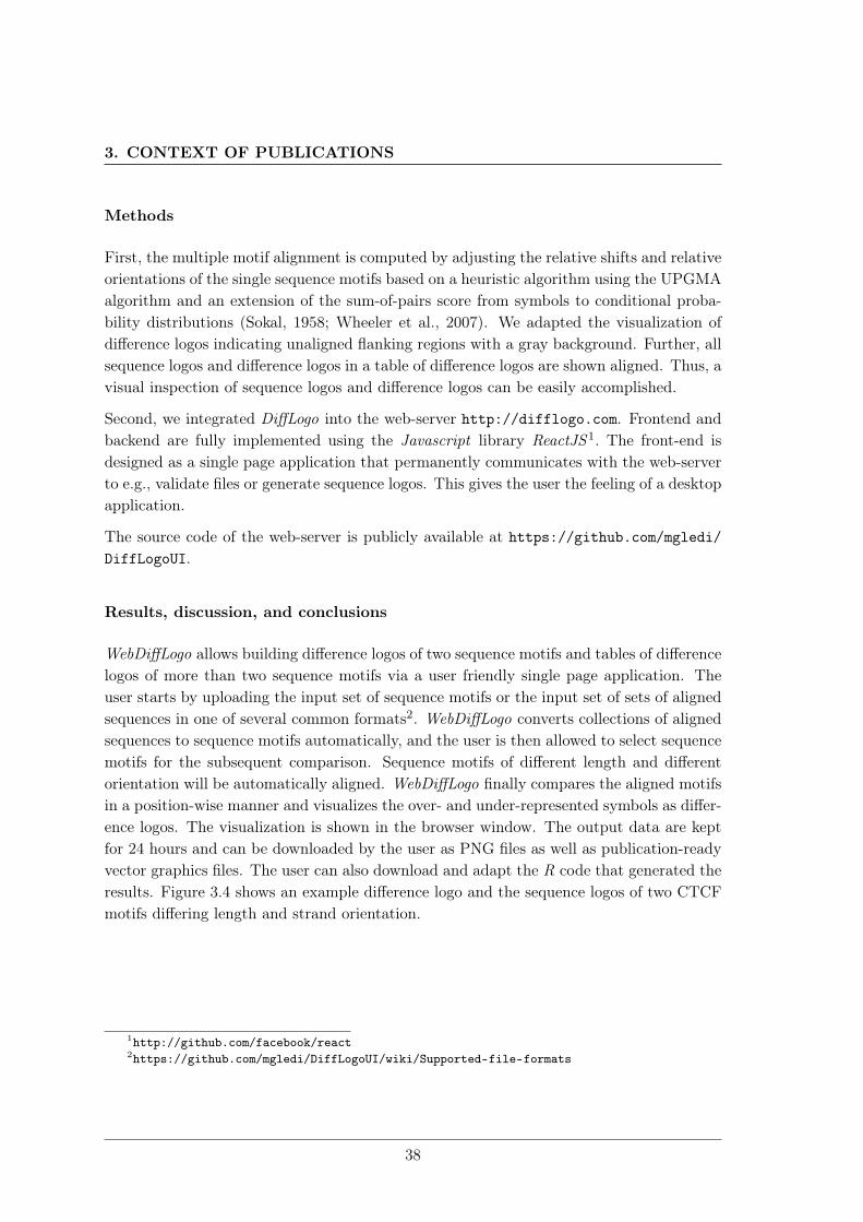
3. CONTEXT OF PUBLICATIONS

Methods

First, the multiple motif alignment is computed by adjusting the relative shifts and relativeorientations of the single sequence motifs based on a heuristic algorithm using the UPGMAalgorithm and an extension of the sum-of-pairs score from symbols to conditional proba-bility distributions (Sokal, 1958; Wheeler et al., 2007). We adapted the visualization ofdifference logos indicating unaligned flanking regions with a gray background. Further, allsequence logos and difference logos in a table of difference logos are shown aligned. Thus, avisual inspection of sequence logos and difference logos can be easily accomplished.

Second, we integrated DiffLogo into the web-server http://difflogo.com. Frontend andbackend are fully implemented using the Javascript library ReactJS 1. The front-end isdesigned as a single page application that permanently communicates with the web-serverto e.g., validate files or generate sequence logos. This gives the user the feeling of a desktopapplication.

The source code of the web-server is publicly available at https://github.com/mgledi/DiffLogoUI.

Results, discussion, and conclusions

WebDiffLogo allows building difference logos of two sequence motifs and tables of differencelogos of more than two sequence motifs via a user friendly single page application. Theuser starts by uploading the input set of sequence motifs or the input set of sets of alignedsequences in one of several common formats2. WebDiffLogo converts collections of alignedsequences to sequence motifs automatically, and the user is then allowed to select sequencemotifs for the subsequent comparison. Sequence motifs of different length and differentorientation will be automatically aligned. WebDiffLogo finally compares the aligned motifsin a position-wise manner and visualizes the over- and under-represented symbols as differ-ence logos. The visualization is shown in the browser window. The output data are keptfor 24 hours and can be downloaded by the user as PNG files as well as publication-readyvector graphics files. The user can also download and adapt the R code that generated theresults. Figure 3.4 shows an example difference logo and the sequence logos of two CTCFmotifs differing length and strand orientation.

1http://github.com/facebook/react2https://github.com/mgledi/DiffLogoUI/wiki/Supported-file-formats

38

Page 49

3.3 Visualization of sequence motifs

Figure 3.4: Difference logo (bottom) and sequence logos of CTCF motifs from celllines H1-hESC (top left) and HUVEC (top right). The H1-hESC motif is two basesshorter than the HUVEC motif. The two motifs also differ in their strand orientation. Theresulting difference logo depicts the small differences of the aligned motifs. Unaligned regionsare indicated with gray background.

39

Page 50

3. CONTEXT OF PUBLICATIONS

3.4 Conclusions and outlook

In this thesis, my colleagues and I have addressed six limitations in three related fields.

First, we proposed miRGen and DRUMS, two approaches to improve “data acquisition anddata preparation.” Specifically, by providing access to over 800miRNA transcripts enrichedwith information about TFBSs near their TSS, with miRNA expression profiles, and withSNPs, miRGen improves the insights into the involvement of miRNAs in gene regulationand thus contributes to cancer diagnostics and therapeutics. Further, DRUMS is a key-value store optimized to handle psDrd running on standard desktop hardware. DRUMSis considerably faster than MySQL by a factor of 2 up to a factor of 15456 regarding thiskind of data.

In comparison to many other NoSQL databases, neither is DRUMS horizontally scalablenor does it support redundancy. It would be an interesting follow-up project to investigateif the DRUMS concept could be extended by those capabilities.

Second, we proposed three approaches to improve “de–novo motif discovery using phyloge-netic footprinting.” Specifically, we found that it is possible to detect and correct the BAbias using inter–species information and that taking into account this bias leads to a moreprecise prediction of TFBSs using phylogenetic footprinting on ChIP-seq data. Further, wefound that phylogenetic footprinting using a star topology with unrealistic high substitu-tion probabilities seem to be more robust toward violation of model assumptions caused byevolutionary effects like heterogeneous and heterotachious substitution probabilities. Fi-nally, we found that combining phylogenetic footprinting with motif models incorporatingintra–motif dependencies lead to an improved prediction of TFBSs. Each of these findingsadvance our attempt of understanding transcriptional gene regulation as a whole.

Regarding “De–novo motif discovery using phylogenetic footprinting,” I propose the follow-ing future works. It would be interesting to investigate more complex evolutionary modelslike the HKY model or the GTR model with the phylogenetic footprinting approachesproposed in this thesis . Further, it seems promising to combine the phylogenetic foot-printing approaches proposed in this thesis to one approach that is capable of detectingand correcting the BA bias and to model intra-motif dependencies. Finally, a combinationof phylogenetic footprinting with more complex motif models like parsimonious Markovmodels or Bayesian Markov models could improve de–novo motif discovery based on phy-logenetic footprinting (Eggeling et al., 2015; Siebert et al., 2016).

Third, we proposed DiffLogo to improve “visualisation of sequence motifs.” DiffLogo is anR package publicly available via Bioconductor1 or GitHub2, developed for the comparative

1http://bioconductor.org/packages/release/bioc/html/DiffLogo.html2http://github.com/mgledi/DiffLogo

40

Page 51

3.4 Conclusions and outlook

visualization of sequence motifs. DiffLogo was downloaded more than 100 times per monthand more than 1000 times in total in 2016. To make DiffLogo applicable to a broader user-ship, we integrated the R package into the easy-to-use web-server WebDiffLogo1. DiffLogoand WebDiffLogo facilitate decision making, knowledge sharing, and the presentation ofresults.

An interesting extension of DiffLogo could be the higher order comparative visualizationof sequence motifs, i.e., the comparative visualization of intra–motif dependencies. Aninteresting follow-up of WebDiffLogo could be a web-server that allows the investigation ofsequence motifs with several existing tools like IceLogo, motifStack, or Two Sample Logo(Colaert et al., 2009; Jianhong Ou, 2014; Vacic et al., 2006). Additionally, the investigationof sequence motifs could be dramatically improved by allowing user interactions with theresults, e.g., investigating only a few motif positions of interest.

1http://difflogo.com

41

Page 52

3. CONTEXT OF PUBLICATIONS

42

Page 53

GlossaryAUC area under receiver operating character-

istics curve.

BA bias binding affinity bias.

bp base pair.

ChIP-seq ChIP-sequencing.

DNA Deoxyribonucleic acid.

DRUM Disk Repository with Update Man-agement.

DRUMS Disk Repository with Update Man-agement and Select option.

EM Expectation Maximization.

F81 evolutionary model Felsenstein 81.

HERV human endogenous retrovirus.

hMM(k) homogeneous Markov model oforder k.

iMM(k) inhomogeneous Markov model oforder k.

KLD Kullback—Leibler divergence.

miRNA microRNA.

mRNA messenger RNA.

MSA multiple sequence alignment.

mutual information mutual information.

NoSQL not only SQL.

PFM phylogenetic footprinting model.

PR precision recall.

psDrd position-specific DNA related data.

PWM position weight matrix.

RISC RNA-Induced Silencing Complex.

RNA Ribonucleic acid.

ROC receiver operating characteristics.

SNP single nucleotide polymorphism.

SQL structured query language.

TF transcription factor.

TFBS transcription factor binding site.

TSS transcription start site.

UTR untranslated region.

ZOOPS zero or one occurrence of a bindingsite per sequence.

43

Page 54

Glossary

44

Page 55

ReferencesAgostini, Federico, Davide Cirillo, Riccardo D Ponti, and Gian G Tartaglia (2014). SeAMotE:

a method for high-throughput motif discovery in nucleic acid sequences. BMC genomics,15 (1), p. 925.

Alexiou, Panagiotis, Thanasis Vergoulis, Martin Gleditzsch, George Prekas, Theodore Dala-magas, Molly Megraw, Ivo Grosse, Timos Sellis, and Artemis G Hatzigeorgiou (2009).miRGen 2.0: a database of microRNA genomic information and regulation. Nucleicacids research, gkp888.

Alipanahi, Babak, Andrew Delong, Matthew T. Weirauch, and Brendan J. Frey (2015).Predicting the sequence specificities of DNA- and RNA-binding proteins by deep learn-ing. Nature Biotechnology, 33 (8), pp. 831–838.

Arnold, Phil, Ionas Erb, Mikhail Pachkov, Nacho Molina, and Erik van Nimwegen (2012).MotEvo: integrated Bayesian probabilistic methods for inferring regulatory sites andmotifs on multiple alignments of DNA sequences. Bioinformatics, 28 (4), pp. 487–494.

Bailey, Timothy L. and Charles Elkan (1995). “The value of prior knowledge in discoveringmotifs with MEME.” In: ISMB. International Conference on Intelligent Systems forMolecular Biology. Vol. 3, pp. 21–29.

Bailey, Timothy L., Pawel Krajewski, Istvan Ladunga, Celine Lefebvre, Qunhua Li, TaoLiu, Pedro Madrigal, Cenny Taslim, and Jie Zhang (2013). Practical guidelines for thecomprehensive analysis of ChIP-seq data. PLoS computational biology, 9 (11).

Bailey, Timothy, Pawel Krajewski, Istvan Ladunga, Celine Lefebvre, Qunhua Li, Tao Liu,Pedro Madrigal, Cenny Taslim, and Jie Zhang (2013). Practical guidelines for the com-prehensive analysis of ChIP-seq data. PLoS Comput Biol, 9 (11), e1003326.

Bembom, Oliver. seqLogo: Sequence logos for DNA sequence alignments. R package version1.28.0. Division of Biostatistics, University of California, Berkeley.

Blanchette, Mathieu and Martin Tompa (2003). FootPrinter: a program designed for phy-logenetic footprinting. Nucleic acids research, 31 (13), pp. 3840–3842.

Bourgon, Richard, Robert Gentleman, and Wolfgang Huber (2010). Independent filteringincreases detection power for high-throughput experiments. Proceedings of the NationalAcademy of Sciences, 107 (21), pp. 9546–9551.

Bulyk, Martha (2003). Computational prediction of transcription-factor binding site loca-tions. Genome Biology, 5 (1), pp. 201+.

Bulyk, Martha L, Philip LF Johnson, and George M Church (2002). Nucleotides of tran-scription factor binding sites exert interdependent effects on the binding affinities oftranscription factors. Nucleic acids research, 30 (5), pp. 1255–1261.

45

Page 56

REFERENCES

Calin, George A and Carlo M Croce (2006). MicroRNA signatures in human cancers.Nature Reviews Cancer, 6 (11), pp. 857–866.

Carrington, James C and Victor Ambros (2003). Role of microRNAs in plant and animaldevelopment. Science, 301 (5631), pp. 336–338.

Chen, Kevin and Nikolaus Rajewsky (2007). The evolution of gene regulation by transcrip-tion factors and microRNAs. Nature Reviews Genetics, 8 (2), pp. 93–103.

Clark, Andrew G, Michael B Eisen, Douglas R Smith, Casey M Bergman, Brian Oliver,Therese A Markow, Thomas C Kaufman, Manolis Kellis, William Gelbart, Venky NIyer, et al. (2007). Evolution of genes and genomes on the Drosophila phylogeny. Nature,450 (7167), pp. 203–218.

Codd, Edgar F (1970). A relational model of data for large shared data banks. Communi-cations of the ACM, 13 (6), pp. 377–387.

Colaert, Niklaas, Kenny Helsens, Lennart Martens, Joel Vandekerckhove, and Kris Gevaert(2009). Improved visualization of protein consensus sequences by iceLogo. Nature meth-ods, 6 (11), pp. 786–787.

Consortium, 1000 Genomes Project et al. (2012). An integrated map of genetic variationfrom 1,092 human genomes. Nature, 491 (7422), pp. 56–65.

Consortium, ENCODE Project et al. (2004). The ENCODE (ENCyclopedia of DNA ele-ments) project. Science, 306 (5696), pp. 636–640.

— (2012). An integrated encyclopedia of DNA elements in the human genome. Nature,489 (7414), pp. 57–74.

Crick, Francis et al. (1970). Central dogma of molecular biology. Nature, 227 (5258),pp. 561–563.

Darwin, Charles (1859). On the origin of species.D’haeseleer, Patrik (2006). How does DNA sequence motif discovery work? Nature biotech-

nology, 24 (8), pp. 959–961.Dolinoy, Dana C, Jennifer R Weidman, and Randy L Jirtle (2007). Epigenetic gene regula-

tion: linking early developmental environment to adult disease. Reproductive Toxicology,23 (3), pp. 297–307.

Dragland, Åse (2013). Big Data, for better or worse: 90% of world’s data generated over lasttwo years. url: https://www.sciencedaily.com/releases/2013/05/130522085217.htm (visited on 12/10/2016).

Durinck, Steffen, Yves Moreau, Arek Kasprzyk, Sean Davis, Bart De Moor, Alvis Brazma,and Wolfgang Huber (2005). BioMart and Bioconductor: a powerful link between bi-ological databases and microarray data analysis. Bioinformatics, 21 (16), pp. 3439–3440.

Eggeling, Ralf, Teemu Roos, Petri Myllymäki, and Ivo Grosse (2015). Inferring intra-motifdependencies of DNA binding sites from ChIP-seq data. BMC bioinformatics, 16 (1),p. 375.

46

Page 57

REFERENCES

Elliott, Julian H., Jeremy Grimshaw, Russ Altman, Lisa Bero, Steven N. Goodman, DavidHenry, Malcolm Macleod, David Tovey, Peter Tugwell, Howard White, and Ida Sim(2015). Informatics: Make sense of health data. Nature, 527, pp. 31–32.

Farazi, Thalia A, Jessica I Spitzer, Pavel Morozov, and Thomas Tuschl (2011). miRNAsin human cancer. The Journal of pathology, 223 (2), pp. 102–115.

Felsenstein, Jospeh (1981). Evolutionary trees from DNA sequences: a maximum likelihoodapproach. Journal of Molecular Evolution, 17 (6), pp. 368–376.

Fougerolles, Antonin de, Hans-Peter Vornlocher, John Maraganore, and Judy Lieberman(2007). Interfering with disease: a progress report on siRNA-based therapeutics. Naturereviews Drug discovery, 6 (6), pp. 443–453.

Fredslund, Jakob (2006). PHY·FI: fast and easy online creation and manipulation of phy-logeny color figures. BMC bioinformatics, 7 (1), p. 1.

Furey, Terrence S. (2012). ChIP-seq and beyond: new and improved methodologies todetect and characterize protein-DNA interactions. Nature Reviews Genetics, 13 (12),pp. 840–852.

Gantz, John and David Reinsel (2012). The digital universe in 2020: Big data, bigger digitalshadows, and biggest growth in the far east. IDC iView: IDC Analyze the future, 2007,pp. 1–16.

Gentleman, Robert C, Vincent J Carey, Douglas M Bates, Ben Bolstad, Marcel Dettling,Sandrine Dudoit, Byron Ellis, Laurent Gautier, Yongchao Ge, Jeff Gentry, et al. (2004).Bioconductor: open software development for computational biology and bioinformat-ics. Genome biology, 5 (10), R80.

Gertz, Jason, Justin C. Fay, and Barak A. Cohen (2006). Phylogeny based discovery ofregulatory elements. BMC Bioinformatics, 7, p. 266.

Gomes, Antonio LC, Thomas Abeel, Matthew Peterson, Elham Azizi, Anna Lyubetskaya,Luís Carvalho, and James Galagan (2014). Decoding ChIP-seq with a double-bindingsignal refines binding peaks to single-nucleotides and predicts cooperative interaction.Genome research, 24 (10), pp. 1686–1697.

Gosling, James, Bill Joy, Guy L Steele, Gilad Bracha, and Alex Buckley (2014). The JavaLanguage Specification. Pearson Education.

Grau, Jan, Jens Keilwagen, André Gohr, Berit Haldemann, Stefan Posch, and Ivo Grosse(2012). Jstacs: A Java framework for statistical analysis and classification of biologicalsequences. Journal of Machine Learning Research, 13 (Jun), pp. 1967–1971.

Grau, Jan, Stefan Posch, Ivo Grosse, and Jens Keilwagen (2013). A general approachfor discriminative de novo motif discovery from high-throughput data. Nucleic acidsresearch, gkt831.

Håndstad, Tony, Morten B. Rye, Finn Drabløs, and Pål Sætrom (2011). A ChIP-SeqBenchmark Shows That Sequence Conservation Mainly Improves Detection of StrongTranscription Factor Binding Sites. PLoS ONE, 6 (4), e18430+.

47

Page 58

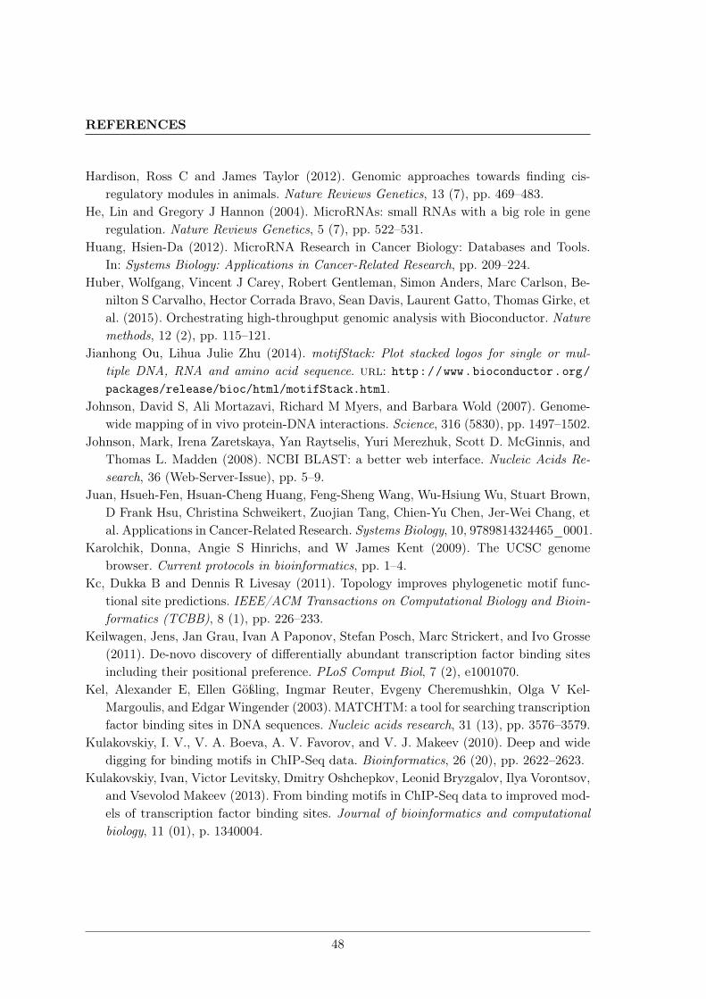
REFERENCES

Hardison, Ross C and James Taylor (2012). Genomic approaches towards finding cis-regulatory modules in animals. Nature Reviews Genetics, 13 (7), pp. 469–483.

He, Lin and Gregory J Hannon (2004). MicroRNAs: small RNAs with a big role in generegulation. Nature Reviews Genetics, 5 (7), pp. 522–531.

Huang, Hsien-Da (2012). MicroRNA Research in Cancer Biology: Databases and Tools.In: Systems Biology: Applications in Cancer-Related Research, pp. 209–224.

Huber, Wolfgang, Vincent J Carey, Robert Gentleman, Simon Anders, Marc Carlson, Be-nilton S Carvalho, Hector Corrada Bravo, Sean Davis, Laurent Gatto, Thomas Girke, etal. (2015). Orchestrating high-throughput genomic analysis with Bioconductor. Naturemethods, 12 (2), pp. 115–121.

Jianhong Ou, Lihua Julie Zhu (2014). motifStack: Plot stacked logos for single or mul-tiple DNA, RNA and amino acid sequence. url: http://www.bioconductor.org/packages/release/bioc/html/motifStack.html.

Johnson, David S, Ali Mortazavi, Richard M Myers, and Barbara Wold (2007). Genome-wide mapping of in vivo protein-DNA interactions. Science, 316 (5830), pp. 1497–1502.

Johnson, Mark, Irena Zaretskaya, Yan Raytselis, Yuri Merezhuk, Scott D. McGinnis, andThomas L. Madden (2008). NCBI BLAST: a better web interface. Nucleic Acids Re-search, 36 (Web-Server-Issue), pp. 5–9.

Juan, Hsueh-Fen, Hsuan-Cheng Huang, Feng-Sheng Wang, Wu-Hsiung Wu, Stuart Brown,D Frank Hsu, Christina Schweikert, Zuojian Tang, Chien-Yu Chen, Jer-Wei Chang, etal. Applications in Cancer-Related Research. Systems Biology, 10, 9789814324465_0001.

Karolchik, Donna, Angie S Hinrichs, and W James Kent (2009). The UCSC genomebrowser. Current protocols in bioinformatics, pp. 1–4.

Kc, Dukka B and Dennis R Livesay (2011). Topology improves phylogenetic motif func-tional site predictions. IEEE/ACM Transactions on Computational Biology and Bioin-formatics (TCBB), 8 (1), pp. 226–233.

Keilwagen, Jens, Jan Grau, Ivan A Paponov, Stefan Posch, Marc Strickert, and Ivo Grosse(2011). De-novo discovery of differentially abundant transcription factor binding sitesincluding their positional preference. PLoS Comput Biol, 7 (2), e1001070.

Kel, Alexander E, Ellen Gößling, Ingmar Reuter, Evgeny Cheremushkin, Olga V Kel-Margoulis, and Edgar Wingender (2003). MATCHTM: a tool for searching transcriptionfactor binding sites in DNA sequences. Nucleic acids research, 31 (13), pp. 3576–3579.

Kulakovskiy, I. V., V. A. Boeva, A. V. Favorov, and V. J. Makeev (2010). Deep and widedigging for binding motifs in ChIP-Seq data. Bioinformatics, 26 (20), pp. 2622–2623.

Kulakovskiy, Ivan, Victor Levitsky, Dmitry Oshchepkov, Leonid Bryzgalov, Ilya Vorontsov,and Vsevolod Makeev (2013). From binding motifs in ChIP-Seq data to improved mod-els of transcription factor binding sites. Journal of bioinformatics and computationalbiology, 11 (01), p. 1340004.

48

Page 59

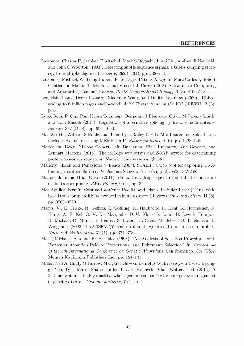
REFERENCES

Lawrence, Charles E, Stephen F Altschul, Mark S Boguski, Jun S Liu, Andrew F Neuwald,and John C Wootton (1993). Detecting subtle sequence signals: a Gibbs sampling strat-egy for multiple alignment. science, 262 (5131), pp. 208–214.

Lawrence, Michael, Wolfgang Huber, Hervé Pagès, Patrick Aboyoun, Marc Carlson, RobertGentleman, Martin T. Morgan, and Vincent J. Carey (2013). Software for Computingand Annotating Genomic Ranges. PLOS Computational Biology, 9 (8), e1003118+.

Lee, Hsin-Tsang, Derek Leonard, Xiaoming Wang, and Dmitri Loguinov (2009). IRLbot:scaling to 6 billion pages and beyond. ACM Transactions on the Web (TWEB), 3 (3),p. 8.

Luco, Reini F, Qun Pan, Kaoru Tominaga, Benjamin J Blencowe, Olivia M Pereira-Smith,and Tom Misteli (2010). Regulation of alternative splicing by histone modifications.Science, 327 (5968), pp. 996–1000.

Ma, Wenxiu, William S Noble, and Timothy L Bailey (2014). Motif-based analysis of largenucleotide data sets using MEME-ChIP. Nature protocols, 9 (6), pp. 1428–1450.

Maddelein, Davy, Niklaas Colaert, Iain Buchanan, Niels Hulstaert, Kris Gevaert, andLennart Martens (2015). The iceLogo web server and SOAP service for determiningprotein consensus sequences. Nucleic acids research, gkv385.

Mahony, Shaun and Panayiotis V Benos (2007). STAMP: a web tool for exploring DNA-binding motif similarities. Nucleic acids research, 35 (suppl 2), W253–W258.

Malone, John and Brian Oliver (2011). Microarrays, deep sequencing and the true measureof the transcriptome. BMC Biology, 9 (1), pp. 34+.

Mar-Aguilar, Fermín, Cristina Rodríguez-Padilla, and Diana Reséndez-Pérez (2016). Web-based tools for microRNAs involved in human cancer (Review).Oncology Letters, 11 (6),pp. 3563–3570.

Matys, V., E. Fricke, R. Geffers, E. Gößling, M. Haubrock, R. Hehl, K. Hornischer, D.Karas, A. E. Kel, O. V. Kel-Margoulis, D.-U. Kloos, S. Land, B. Lewicki-Potapov,H. Michael, R. Münch, I. Reuter, S. Rotert, H. Saxel, M. Scheer, S. Thiele, and E.Wingender (2003). TRANSFAC R©: transcriptional regulation, from patterns to profiles.Nucleic Acids Research, 31 (1), pp. 374–378.

Maza, Michael de la and Bruce Tidor (1993). “An Analysis of Selection Procedures withParticular Attention Paid to Proportional and Boltzmann Selection”. In: Proceedingsof the 5th International Conference on Genetic Algorithms. San Francisco, CA, USA:Morgan Kaufmann Publishers Inc., pp. 124–131.

Miller, Neil A, Emily G Farrow, Margaret Gibson, Laurel K Willig, Greyson Twist, Byung-gil Yoo, Tyler Marrs, Shane Corder, Lisa Krivohlavek, Adam Walter, et al. (2015). A26-hour system of highly sensitive whole genome sequencing for emergency managementof genetic diseases. Genome medicine, 7 (1), p. 1.

49

Page 60

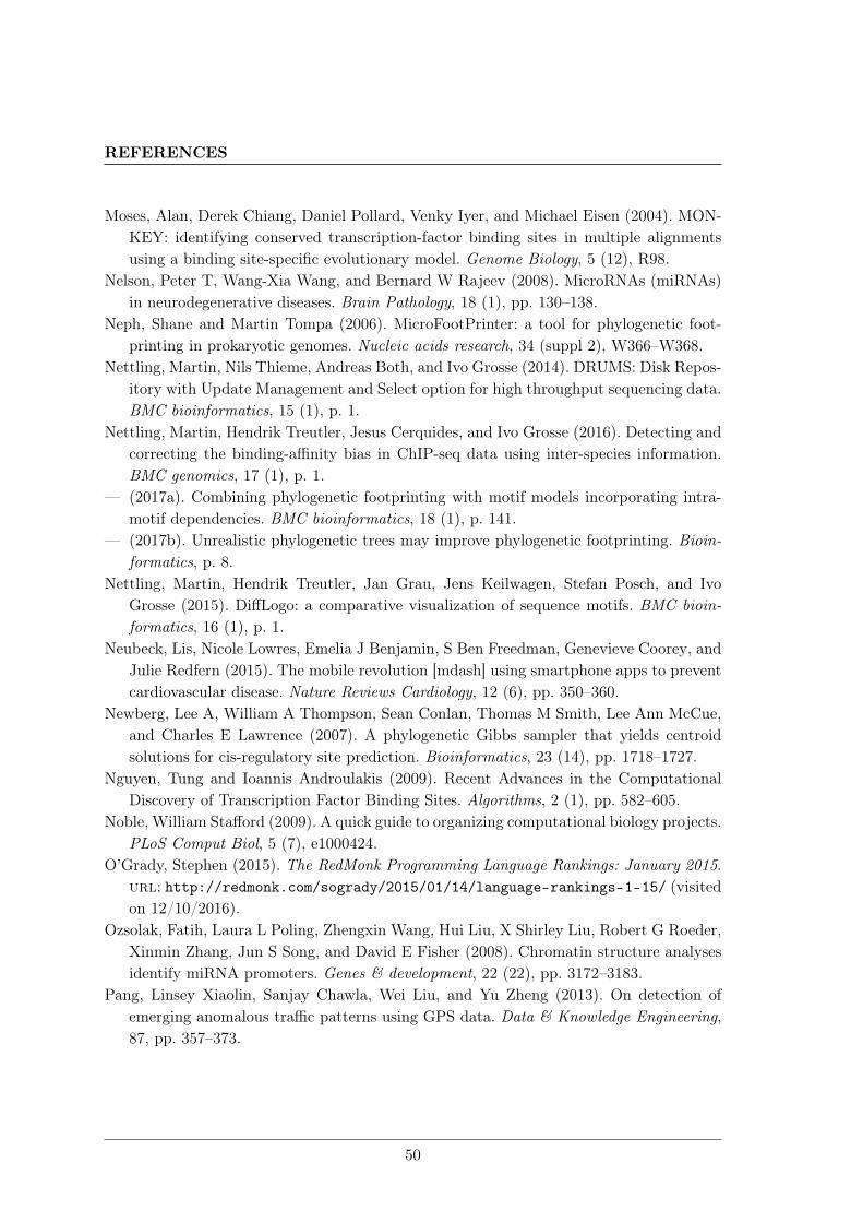
REFERENCES

Moses, Alan, Derek Chiang, Daniel Pollard, Venky Iyer, and Michael Eisen (2004). MON-KEY: identifying conserved transcription-factor binding sites in multiple alignmentsusing a binding site-specific evolutionary model. Genome Biology, 5 (12), R98.

Nelson, Peter T, Wang-Xia Wang, and Bernard W Rajeev (2008). MicroRNAs (miRNAs)in neurodegenerative diseases. Brain Pathology, 18 (1), pp. 130–138.

Neph, Shane and Martin Tompa (2006). MicroFootPrinter: a tool for phylogenetic foot-printing in prokaryotic genomes. Nucleic acids research, 34 (suppl 2), W366–W368.

Nettling, Martin, Nils Thieme, Andreas Both, and Ivo Grosse (2014). DRUMS: Disk Repos-itory with Update Management and Select option for high throughput sequencing data.BMC bioinformatics, 15 (1), p. 1.

Nettling, Martin, Hendrik Treutler, Jesus Cerquides, and Ivo Grosse (2016). Detecting andcorrecting the binding-affinity bias in ChIP-seq data using inter-species information.BMC genomics, 17 (1), p. 1.

— (2017a). Combining phylogenetic footprinting with motif models incorporating intra-motif dependencies. BMC bioinformatics, 18 (1), p. 141.

— (2017b). Unrealistic phylogenetic trees may improve phylogenetic footprinting. Bioin-formatics, p. 8.

Nettling, Martin, Hendrik Treutler, Jan Grau, Jens Keilwagen, Stefan Posch, and IvoGrosse (2015). DiffLogo: a comparative visualization of sequence motifs. BMC bioin-formatics, 16 (1), p. 1.

Neubeck, Lis, Nicole Lowres, Emelia J Benjamin, S Ben Freedman, Genevieve Coorey, andJulie Redfern (2015). The mobile revolution [mdash] using smartphone apps to preventcardiovascular disease. Nature Reviews Cardiology, 12 (6), pp. 350–360.

Newberg, Lee A, William A Thompson, Sean Conlan, Thomas M Smith, Lee Ann McCue,and Charles E Lawrence (2007). A phylogenetic Gibbs sampler that yields centroidsolutions for cis-regulatory site prediction. Bioinformatics, 23 (14), pp. 1718–1727.

Nguyen, Tung and Ioannis Androulakis (2009). Recent Advances in the ComputationalDiscovery of Transcription Factor Binding Sites. Algorithms, 2 (1), pp. 582–605.

Noble, William Stafford (2009). A quick guide to organizing computational biology projects.PLoS Comput Biol, 5 (7), e1000424.

O’Grady, Stephen (2015). The RedMonk Programming Language Rankings: January 2015.url: http://redmonk.com/sogrady/2015/01/14/language-rankings-1-15/ (visitedon 12/10/2016).

Ozsolak, Fatih, Laura L Poling, Zhengxin Wang, Hui Liu, X Shirley Liu, Robert G Roeder,Xinmin Zhang, Jun S Song, and David E Fisher (2008). Chromatin structure analysesidentify miRNA promoters. Genes & development, 22 (22), pp. 3172–3183.

Pang, Linsey Xiaolin, Sanjay Chawla, Wei Liu, and Yu Zheng (2013). On detection ofemerging anomalous traffic patterns using GPS data. Data & Knowledge Engineering,87, pp. 357–373.

50

Page 61

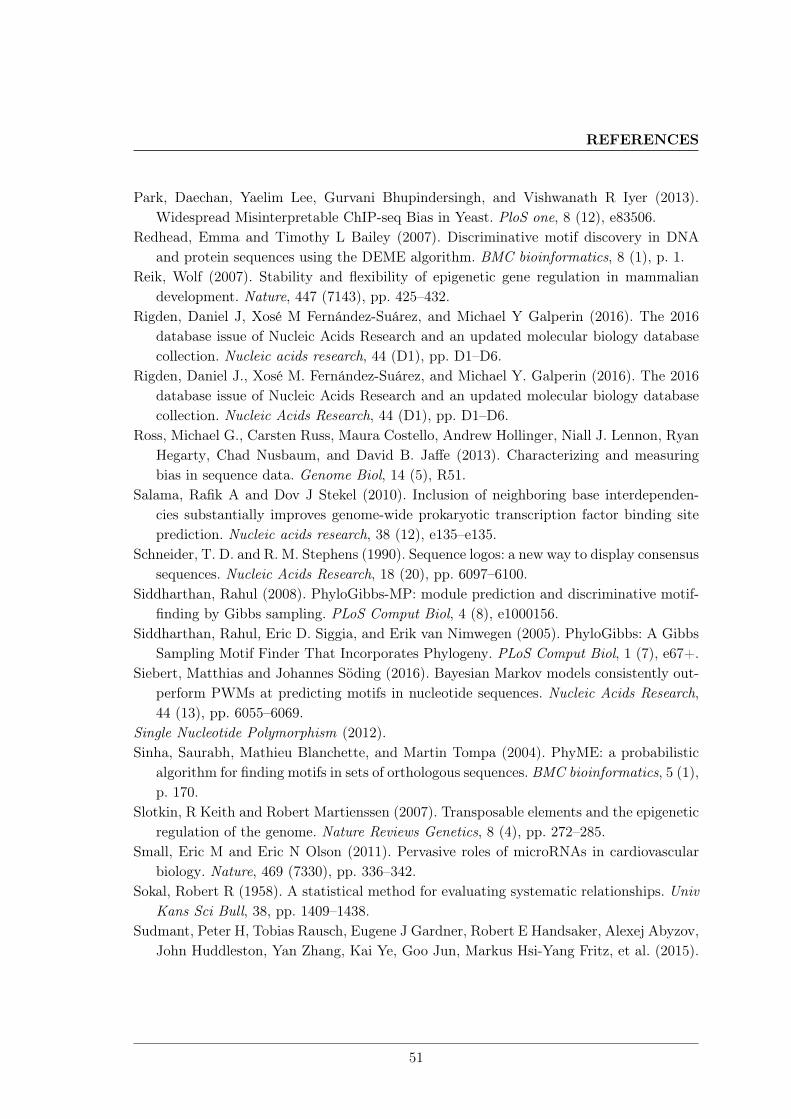
REFERENCES

Park, Daechan, Yaelim Lee, Gurvani Bhupindersingh, and Vishwanath R Iyer (2013).Widespread Misinterpretable ChIP-seq Bias in Yeast. PloS one, 8 (12), e83506.

Redhead, Emma and Timothy L Bailey (2007). Discriminative motif discovery in DNAand protein sequences using the DEME algorithm. BMC bioinformatics, 8 (1), p. 1.

Reik, Wolf (2007). Stability and flexibility of epigenetic gene regulation in mammaliandevelopment. Nature, 447 (7143), pp. 425–432.

Rigden, Daniel J, Xosé M Fernández-Suárez, and Michael Y Galperin (2016). The 2016database issue of Nucleic Acids Research and an updated molecular biology databasecollection. Nucleic acids research, 44 (D1), pp. D1–D6.

Rigden, Daniel J., Xosé M. Fernández-Suárez, and Michael Y. Galperin (2016). The 2016database issue of Nucleic Acids Research and an updated molecular biology databasecollection. Nucleic Acids Research, 44 (D1), pp. D1–D6.

Ross, Michael G., Carsten Russ, Maura Costello, Andrew Hollinger, Niall J. Lennon, RyanHegarty, Chad Nusbaum, and David B. Jaffe (2013). Characterizing and measuringbias in sequence data. Genome Biol, 14 (5), R51.

Salama, Rafik A and Dov J Stekel (2010). Inclusion of neighboring base interdependen-cies substantially improves genome-wide prokaryotic transcription factor binding siteprediction. Nucleic acids research, 38 (12), e135–e135.

Schneider, T. D. and R. M. Stephens (1990). Sequence logos: a new way to display consensussequences. Nucleic Acids Research, 18 (20), pp. 6097–6100.

Siddharthan, Rahul (2008). PhyloGibbs-MP: module prediction and discriminative motif-finding by Gibbs sampling. PLoS Comput Biol, 4 (8), e1000156.

Siddharthan, Rahul, Eric D. Siggia, and Erik van Nimwegen (2005). PhyloGibbs: A GibbsSampling Motif Finder That Incorporates Phylogeny. PLoS Comput Biol, 1 (7), e67+.

Siebert, Matthias and Johannes Söding (2016). Bayesian Markov models consistently out-perform PWMs at predicting motifs in nucleotide sequences. Nucleic Acids Research,44 (13), pp. 6055–6069.

Single Nucleotide Polymorphism (2012).Sinha, Saurabh, Mathieu Blanchette, and Martin Tompa (2004). PhyME: a probabilistic

algorithm for finding motifs in sets of orthologous sequences. BMC bioinformatics, 5 (1),p. 170.

Slotkin, R Keith and Robert Martienssen (2007). Transposable elements and the epigeneticregulation of the genome. Nature Reviews Genetics, 8 (4), pp. 272–285.

Small, Eric M and Eric N Olson (2011). Pervasive roles of microRNAs in cardiovascularbiology. Nature, 469 (7330), pp. 336–342.

Sokal, Robert R (1958). A statistical method for evaluating systematic relationships. UnivKans Sci Bull, 38, pp. 1409–1438.

Sudmant, Peter H, Tobias Rausch, Eugene J Gardner, Robert E Handsaker, Alexej Abyzov,John Huddleston, Yan Zhang, Kai Ye, Goo Jun, Markus Hsi-Yang Fritz, et al. (2015).

51

Page 62

REFERENCES

An integrated map of structural variation in 2,504 human genomes. Nature, 526 (7571),pp. 75–81.

Sultan, Marc, Marcel H Schulz, Hugues Richard, Alon Magen, Andreas Klingenhoff, MatthiasScherf, Martin Seifert, Tatjana Borodina, Aleksey Soldatov, Dmitri Parkhomchuk, etal. (2008). A global view of gene activity and alternative splicing by deep sequencingof the human transcriptome. Science, 321 (5891), pp. 956–960.

Tam, Oliver H, Alexei A Aravin, Paula Stein, Angelique Girard, Elizabeth P Murchison, Si-hem Cheloufi, Emily Hodges, Martin Anger, Ravi Sachidanandam, Richard M Schultz,et al. (2008). Pseudogene-derived small interfering RNAs regulate gene expression inmouse oocytes. Nature, 453 (7194), pp. 534–538.

Teytelman, Leonid, Deborah M. Thurtle, Jasper Rine, and Alexander van Oudenaarden(2013). Highly expressed loci are vulnerable to misleading ChIP localization of mul-tiple unrelated proteins. Proceedings of the National Academy of Sciences, 110 (46),pp. 18602–18607.

Tippmann, Sylvia et al. (2015). Programming tools: Adventures with R. Nature, 517 (7532),pp. 109–110.

Tompa, Martin, Nan Li, Timothy L Bailey, George M Church, Bart De Moor, EleazarEskin, Alexander V Favorov, Martin C Frith, Yutao Fu, W James Kent, et al. (2005).Assessing computational tools for the discovery of transcription factor binding sites.Nature biotechnology, 23 (1), pp. 137–144.

Tran, Ngoc Tam L and Chun-Hsi Huang (2014). A survey of motif finding Web tools fordetecting binding site motifs in ChIP-Seq data. Biol Direct, 9 (1), p. 4.

Vacic, Vladimir, Lilia M Iakoucheva, and Predrag Radivojac (2006). Two Sample Logo:a graphical representation of the differences between two sets of sequence alignments.Bioinformatics, 22 (12), pp. 1536–1537.

Wang, Jie, Jiali Zhuang, Sowmya Iyer, XinYing Lin, Troy W Whitfield, Melissa C Greven,Brian G Pierce, Xianjun Dong, Anshul Kundaje, Yong Cheng, et al. (2012). Sequencefeatures and chromatin structure around the genomic regions bound by 119 humantranscription factors. Genome research, 22 (9), pp. 1798–1812.

Wang, Zhong, Mark Gerstein, and Michael Snyder (2009). RNA-Seq: a revolutionary toolfor transcriptomics. Nature reviews. Genetics, 10 (1), pp. 57–63.

Watson, James D, Francis HC Crick, et al. (1953). Molecular structure of nucleic acids.Nature, 171 (4356), pp. 737–738.

Wheeler, Travis J and John D Kececioglu (2007). Multiple alignment by aligning align-ments. Bioinformatics, 23 (13), pp. i559–i568.

Wilbanks, Elizabeth G and Marc T Facciotti (2010). Evaluation of algorithm performancein ChIP-seq peak detection. PloS one, 5 (7), e11471.

52

Page 63

REFERENCES

Wilson, Greg, DA Aruliah, C Titus Brown, Neil P Chue Hong, Matt Davis, Richard TGuy, Steven HD Haddock, Katy Huff, Ian M Mitchell, Mark D Plumbley, et al. (2014).Best practices for scientific computing. PLoS biology, 12 (1), e1001745.

Zambelli, Federico, Graziano Pesole, and Giulio Pavesi (2012). Motif discovery and tran-scription factor binding sites before and after the next-generation sequencing era. Brief-ings in bioinformatics, bbs016.

53

Page 64

REFERENCES

54

Page 65

4 Data acquisition and data preparation

4.1 miRGen 2.0: a database of microRNA genomic informa-tion and regulation

P Alexiou, T Vergoulis, M Gleditzsch, G Prekas, T Dalamagas, M Megraw, I Grosse,T Sellis, AG Hatzigeorgiou. 2009. miRGen 2.0: a database of microRNA genomic informa-tion and regulation. Nucl. Acids Res. 38 (suppl 1): D137-D141. doi:10.1093/nar/gkp888

55

Page 66

miRGen 2.0: a database of microRNA genomicinformation and regulationPanagiotis Alexiou1,2,*, Thanasis Vergoulis3,4, Martin Gleditzsch5, George Prekas4,

Theodore Dalamagas3, Molly Megraw6, Ivo Grosse5, Timos Sellis3,4 and

Artemis G. Hatzigeorgiou1,7,*

1Institute of Molecular Oncology, Biomedical Sciences Research Center ‘Alexander Fleming’, Vari, 2School ofBiology, Aristotle University of Thessaloniki, Thessaloniki, 3Institute for the Management of Information Systems,‘‘Athena’’ Research Center, 4Knowledge and Database Systems Lab, Department of Computer Science, Schoolof Electrical and Computer Engineering, National Technical University of Athens, Athens, Greece, 5Instituteof Computer Science, Martin Luther University Halle-Wittenberg, Halle, Germany, 6Institute for Genome Sciencesand Policy, Duke University, Durham, NC and 7Computer and Information Sciences, University of Pennsylvania,Philadelphia, PA, USA

Received September 15, 2009; Accepted October 4, 2009

ABSTRACT

MicroRNAs are small, non-protein coding RNAmolecules known to regulate the expression ofgenes by binding to the 30UTR region of mRNAs.MicroRNAs are produced from longer transcriptswhich can code for more than one maturemiRNAs. miRGen 2.0 is a database that aims toprovide comprehensive information about theposition of human and mouse microRNA codingtranscripts and their regulation by transcriptionfactors, including a unique compilation of bothpredicted and experimentally supported data.Expression profiles of microRNAs in severaltissues and cell lines, single nucleotide poly-morphism locations, microRNA target predictionon protein coding genes and mapping of miRNAtargets of co-regulated miRNAs on biologicalpathways are also integrated into the databaseand user interface. The miRGen database will becontinuously maintained and freely available athttp://www.microrna.gr/mirgen/.

INTRODUCTION

MicroRNAs (miRNAs) are single-stranded non-codingRNA molecules of �21 nucleotides in length, thatfunction as regulators of gene expression by binding tomessenger RNA (mRNA) molecules and destabilizing

them or inhibiting their translation. They are found tobe implicated in a wide range of physiological molecularprocesses, and their deregulation leads to diversediseases (1–3).MiRNAs are located in intergenic regions or in the

introns of protein coding genes. They are transcribed byRNA Polymerase II as independent transcripts or as partof the transcript of a host gene. Only a small group ofmiRNAs located inside ALU repetitive elements istranscribed by RNA Polymerase III. A miRNA transcriptcan host more than one miRNA and can be severalthousand nucleotides long including introns.A promoter region is located around the transcription

start site (TSS) of a transcript and is regulated by proteinsthat bind to this region. Evidence thus far suggests thatbinding sites for transcription factors (TFs) are similarlydistributed within the promoters of both protein codinggenes and miRNA transcripts (4). MiRNA primarytranscripts (pri-miRNA) are processed in the nucleus toform pre-miRNAs, �70-nucleotide stem–loop structuresalso called miRNA hairpins. These are later processedinto mature miRNAs in the cytoplasm via interactionwith the endonuclease Dicer, which also initiates theformation of the RNA-induced silencing complex(RISC). Since primary transcripts are short lived andpresent only inside the nucleus, it is hard to identifythem with standard molecular techniques.After the Dicer enzyme cleaves the pre-miRNA

stem–loop, two complementary short RNA moleculesare formed, but only one of them—the guiding strand—is predominantly integrated into the RISC complex.

*To whom correspondence should be addressed. Tel: +30 210 9656310 (int. 248); Email: [email protected] may also be addressed to Artemis G. Hatzigeorgiou. Tel: +30 210 9656310 (int. 190); Fax: +30 210 9653934; Email:[email protected]

Published online 22 October 2009 Nucleic Acids Research, 2010, Vol. 38, Database issue D137–D141doi:10.1093/nar/gkp888

� The Author(s) 2009. Published by Oxford University Press.This is an Open Access article distributed under the terms of the Creative Commons Attribution Non-Commercial License (http://creativecommons.org/licenses/by-nc/2.5/uk/) which permits unrestricted non-commercial use, distribution, and reproduction in any medium, provided the original work is properly cited.

4. DATA ACQUISITION AND DATA PREPARATION

56

Page 67

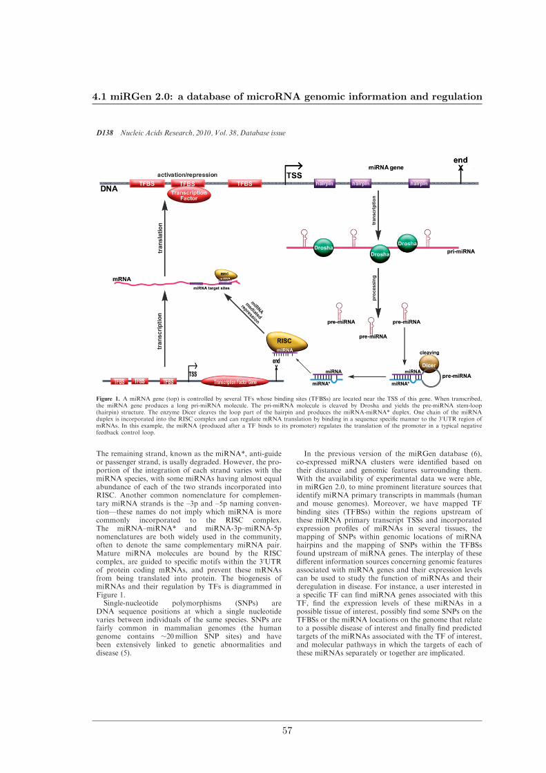
The remaining strand, known as the miRNA*, anti-guideor passenger strand, is usally degraded. However, the pro-portion of the integration of each strand varies with themiRNA species, with some miRNAs having almost equalabundance of each of the two strands incorporated intoRISC. Another common nomenclature for complemen-tary miRNA strands is the –3p and –5p naming conven-tion—these names do not imply which miRNA is morecommonly incorporated to the RISC complex.The miRNA–miRNA* and miRNA-3p–miRNA-5pnomenclatures are both widely used in the community,often to denote the same complementary miRNA pair.Mature miRNA molecules are bound by the RISCcomplex, are guided to specific motifs within the 30UTRof protein coding mRNAs, and prevent these mRNAsfrom being translated into protein. The biogenesis ofmiRNAs and their regulation by TFs is diagrammed inFigure 1.Single-nucleotide polymorphisms (SNPs) are

DNA sequence positions at which a single nucleotidevaries between individuals of the same species. SNPs arefairly common in mammalian genomes (the humangenome contains �20million SNP sites) and havebeen extensively linked to genetic abnormalities anddisease (5).

In the previous version of the miRGen database (6),co-expressed miRNA clusters were identified based ontheir distance and genomic features surrounding them.With the availability of experimental data we were able,in miRGen 2.0, to mine prominent literature sources thatidentify miRNA primary transcripts in mammals (humanand mouse genomes). Moreover, we have mapped TFbinding sites (TFBSs) within the regions upstream ofthese miRNA primary transcript TSSs and incorporatedexpression profiles of miRNAs in several tissues, themapping of SNPs within genomic locations of miRNAhairpins and the mapping of SNPs within the TFBSsfound upstream of miRNA genes. The interplay of thesedifferent information sources concerning genomic featuresassociated with miRNA genes and their expression levelscan be used to study the function of miRNAs and theirderegulation in disease. For instance, a user interested ina specific TF can find miRNA genes associated with thisTF, find the expression levels of these miRNAs in apossible tissue of interest, possibly find some SNPs on theTFBSs or the miRNA locations on the genome that relateto a possible disease of interest and finally find predictedtargets of the miRNAs associated with the TF of interest,and molecular pathways in which the targets of each ofthese miRNAs separately or together are implicated.

Figure 1. A miRNA gene (top) is controlled by several TFs whose binding sites (TFBSs) are located near the TSS of this gene. When transcribed,the miRNA gene produces a long pri-miRNA molecule. The pri-miRNA molecule is cleaved by Drosha and yields the pre-miRNA stem-loop(hairpin) structure. The enzyme Dicer cleaves the loop part of the hairpin and produces the miRNA-miRNA* duplex. One chain of the miRNAduplex is incorporated into the RISC complex and can regulate mRNA translation by binding in a sequence specific manner to the 30UTR region ofmRNAs. In this example, the miRNA (produced after a TF binds to its promoter) regulates the translation of the promoter in a typical negativefeedback control loop.

D138 Nucleic Acids Research, 2010, Vol. 38, Database issue

4.1 miRGen 2.0: a database of microRNA genomic information and regulation

57

Page 68

DATA GENERATION

miRNA coding transcripts

MiRNA transcripts in human and mouse were identifiedfrom four literature sources:

(i) Corcoran et al. (7) used PolII immunoprecipitationdata and ChIP–chip on lung epithelial cells toidentify miRNA transcripts and their promoterregions.

(ii) Landgraf et al. (8) sequenced 250 small RNAlibraries corresponding to 26 different organsystems and cell types of human and mouse, with�1000 miRNA clones per library and identifiedmiRNA coding genes. In this study the wholetranscripts of miRNA coding genes were identified,as well as protein coding genes that containmiRNAs.

(iii) Oszolak et al. (9) predicted the location of the prox-imal promoters of human miRNAs by combiningnucleosome mapping with promoter chromatinsignatures in MALME, HeLa and UACC62 cells.Although the TSS of miRNA genes was identifiedin this study, the end of the transcript was notprovided. We have provided end of the lastmiRNA that is a member of a gene as an approx-imation of the transcript end.

(iv) Marson et al. (10) used ChIP-seq data to identifypromoters of miRNA genes in embryonic stem cells.They identified promoters and co-regulatedmiRNAs, but the exact position of the TSS wasnot identified. For this reason we have used thestart of the first miRNA of each cluster as theputative TSS. Additionally, coordinates providedby Marson et al. had to be lifted over using‘UCSC lift over tool’ to the current genome build(hg18, mm9). In cases where putative rather thanexperimentally verified positions are used, theyare denoted in the graphical interface as ‘computa-tional TSS’.

In total, 812 human miRNA coding transcripts and 386mouse miRNA coding transcripts were identified. Ofthem, 423 were shown in the corresponding papers to beassociated with protein coding genes (intragenic miRNAtranscripts). More than one of the above publicationshave usually identified transcripts corresponding to amiRNA. When this is the case, transcripts from allmethods are returned to the user.

Since these studies were published, additionalmiRNAs have been identified. When novel miRNAsare located within the coordinates of clusters givenby any of these publications, this miRNA is addedto the cluster. For names that changed or were givendifferently than the current standard, manual curationwith reference to mirBase (11) was used to identify andreplace these names according to the current standard.For all the above reasons it is possible that the numberof genes used in miRGen (Table 1) does not correspondperfectly to the number stated in the correspondingpublications.

TFBS identification

In order to determine putative TFBSs near the TSS ofmiRNA primary transcripts, we used the freely availabletool MatchTM (12). MatchTM uses the public library ofposition weight matrices from Transfac 6.0—cite:TRANSFAC: an integrated system for gene expressionregulation. We matched all vertebrate TF matrices tothe regions spanning from 5kb upstream of each TSS to1 kb downstream of the TSS. As criterion for determiningthe cut-off values we chose the minimization of falsepositives in order to produce a strict set of predictionswithout too many falsely predicted TFBSs. Two scoresare calculated for each putative TFBS. The matrix simi-larity score describes the quality of a match between awhole matrix and an arbitrary part of the input sequences.Analogously, the core similarity score denotes the qualityof the match between the core sequence of a matrix(i.e. the five most conserved positions within a matrix)and a part of the input sequence.

miRNA expression profiles

miRNA expression profiles were identified from the mam-malian miRNA expression atlas (8). Information for theexpression profiles of 548 human and 451 mouse miRNAsover 172 human and 68 mouse small RNA libraries werederived from cell lines and tissues.

SNPs

SNPs located within the genomic positions of miRNAhairpins and corresponding TFBSs were downloadedfrom the UCSC table browser (13). For human,Polymorphism data from dbSnp database (14) orgenotyping arrays SNP130 were used with 18 833 531identified SNPs. For mouse, SNP128 was used with14 893 502 identified SNPs.

Implementations

The miRGen repository has been implemented usingrelational database technology. All data are stored ina MySQL relational database management system.Figure 2 illustrates part of the entity-relationship modelof our application. All results are available through a user-friendly interface that allows searches for miRNAs and forTFs of interest. For mature miRNAs, it is possible to viewtargets predicted by the program microT-ANN and formiRNAs found in the same transcript, the user can seea functional annotation of their targets on molecular

Table 1. Number of miRNA coding genes and mature miRNAs

identified in each of the experimental studies used to populate the

miRGen database

References HumanGenes

HumanmiRNA

MouseGenes

MousemiRNA

Corcoran et al. (7) 73 148 – –Landgraf et al. (8) 201 347 191 590Ozsolak et al. (9) 191 268 – –Marson et al. (10) 346 507 195 422

Nucleic Acids Research, 2010, Vol. 38, Database issue D139

4. DATA ACQUISITION AND DATA PREPARATION

58

Page 69

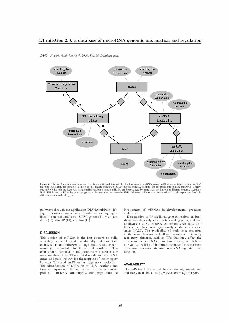
pathways through the application DIANA-mirPath (15).Figure 3 shows an overview of the interface and highlightslinks to external databases—UCSC genome browser (13),iHop (16), dbSNP (14), mirBase (11).

DISCUSSION

This version of miRGen is the first attempt to builda widely accessible and user-friendly database thatconnects TFs and miRNAs through putative and experi-mentally supported functional relationships. Theconnections identified in the database will further ourunderstanding of the TF-mediated regulation of miRNAgenes, and pave the way for the mapping of the interplaybetween TFs and miRNAs as regulatory molecules.The identification of SNPs on miRNA locations andtheir corresponding TFBSs, as well as the expressionprofiles of miRNAs can improve our insight into the

involvement of miRNAs in developmental processesand disease.

Deregulation of TF-mediated gene expression has beenshown to extensively affect protein coding genes, and leadto disease (17,18). MiRNA expression levels have alsobeen shown to change significantly in different diseasestates (19,20). The availability of both these resourcesin the same database will allow researchers to identifyregulatory elements, such as TFs that may affect theexpression of miRNAs. For this reason, we believemiRGen 2.0 will be an important resource for researchersof diverse disciplines interested in miRNA regulation andfunction.

AVAILABILITY

The miRGen database will be continuously maintainedand freely available at http://www.microrna.gr/mirgen/.

Figure 2. The miRGen database schema. TFs (top right) bind through TF binding sites to miRNA genes. miRNA genes (top) contain miRNAhairpins that signify the genomic location of the mature miRNA-miRNA* duplex. miRNA hairpins are processed into mature miRNAs. Usually,one miRNA hairpin produces two mature miRNAs, but a mature miRNA can be produced by more than one hairpin in different genomic locations.Both TFBSs and miRNA hairpins are genomic features that can contain SNPs. Mature miRNAs are associated with their expression levels indifferent tissues and cell types.

D140 Nucleic Acids Research, 2010, Vol. 38, Database issue

4.1 miRGen 2.0: a database of microRNA genomic information and regulation

59

Page 70

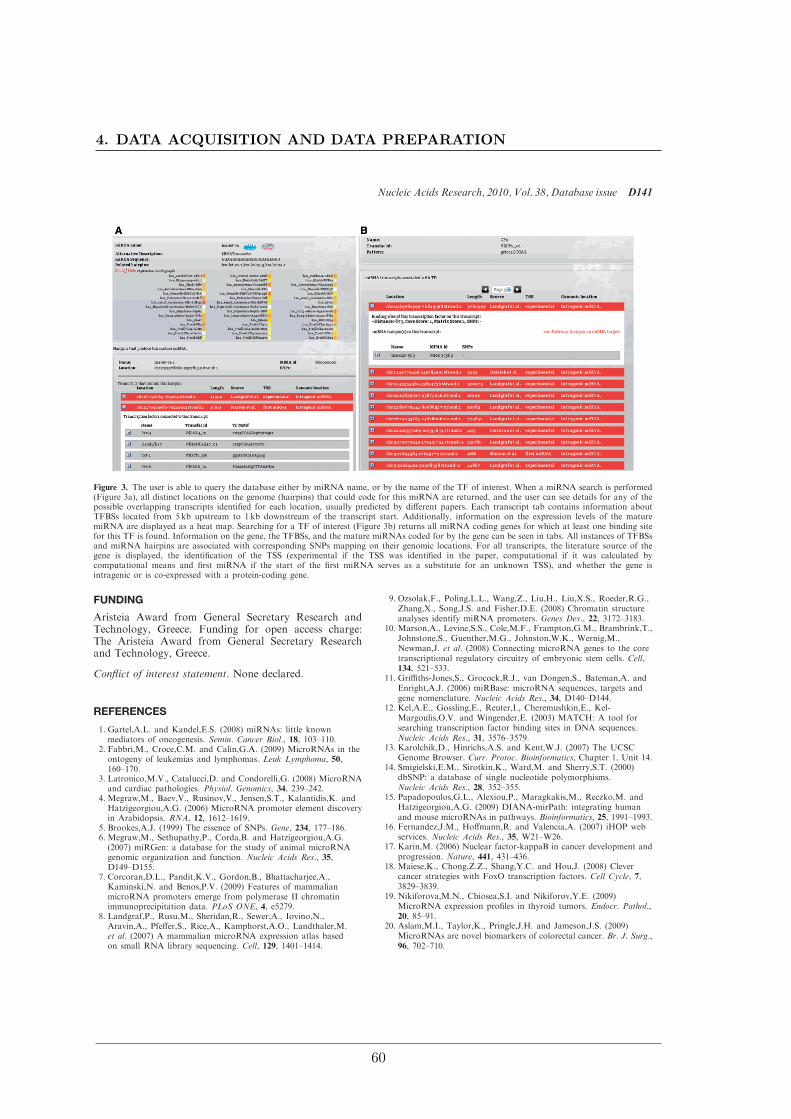
FUNDING

Aristeia Award from General Secretary Research andTechnology, Greece. Funding for open access charge:The Aristeia Award from General Secretary Researchand Technology, Greece.

Conflict of interest statement. None declared.

REFERENCES

1. Gartel,A.L. and Kandel,E.S. (2008) miRNAs: little knownmediators of oncogenesis. Semin. Cancer Biol., 18, 103–110.

2. Fabbri,M., Croce,C.M. and Calin,G.A. (2009) MicroRNAs in theontogeny of leukemias and lymphomas. Leuk Lymphoma, 50,160–170.

3. Latronico,M.V., Catalucci,D. and Condorelli,G. (2008) MicroRNAand cardiac pathologies. Physiol. Genomics, 34, 239–242.

4. Megraw,M., Baev,V., Rusinov,V., Jensen,S.T., Kalantidis,K. andHatzigeorgiou,A.G. (2006) MicroRNA promoter element discoveryin Arabidopsis. RNA, 12, 1612–1619.

5. Brookes,A.J. (1999) The essence of SNPs. Gene, 234, 177–186.6. Megraw,M., Sethupathy,P., Corda,B. and Hatzigeorgiou,A.G.

(2007) miRGen: a database for the study of animal microRNAgenomic organization and function. Nucleic Acids Res., 35,D149–D155.

7. Corcoran,D.L., Pandit,K.V., Gordon,B., Bhattacharjee,A.,Kaminski,N. and Benos,P.V. (2009) Features of mammalianmicroRNA promoters emerge from polymerase II chromatinimmunoprecipitation data. PLoS ONE, 4, e5279.

8. Landgraf,P., Rusu,M., Sheridan,R., Sewer,A., Iovino,N.,Aravin,A., Pfeffer,S., Rice,A., Kamphorst,A.O., Landthaler,M.et al. (2007) A mammalian microRNA expression atlas basedon small RNA library sequencing. Cell, 129, 1401–1414.

9. Ozsolak,F., Poling,L.L., Wang,Z., Liu,H., Liu,X.S., Roeder,R.G.,Zhang,X., Song,J.S. and Fisher,D.E. (2008) Chromatin structureanalyses identify miRNA promoters. Genes Dev., 22, 3172–3183.

10. Marson,A., Levine,S.S., Cole,M.F., Frampton,G.M., Brambrink,T.,Johnstone,S., Guenther,M.G., Johnston,W.K., Wernig,M.,Newman,J. et al. (2008) Connecting microRNA genes to the coretranscriptional regulatory circuitry of embryonic stem cells. Cell,134, 521–533.

11. Griffiths-Jones,S., Grocock,R.J., van Dongen,S., Bateman,A. andEnright,A.J. (2006) miRBase: microRNA sequences, targets andgene nomenclature. Nucleic Acids Res., 34, D140–D144.

12. Kel,A.E., Gossling,E., Reuter,I., Cheremushkin,E., Kel-Margoulis,O.V. and Wingender,E. (2003) MATCH: A tool forsearching transcription factor binding sites in DNA sequences.Nucleic Acids Res., 31, 3576–3579.

13. Karolchik,D., Hinrichs,A.S. and Kent,W.J. (2007) The UCSCGenome Browser. Curr. Protoc. Bioinformatics, Chapter 1, Unit 14.

14. Smigielski,E.M., Sirotkin,K., Ward,M. and Sherry,S.T. (2000)dbSNP: a database of single nucleotide polymorphisms.Nucleic Acids Res., 28, 352–355.

15. Papadopoulos,G.L., Alexiou,P., Maragkakis,M., Reczko,M. andHatzigeorgiou,A.G. (2009) DIANA-mirPath: integrating humanand mouse microRNAs in pathways. Bioinformatics, 25, 1991–1993.

16. Fernandez,J.M., Hoffmann,R. and Valencia,A. (2007) iHOP webservices. Nucleic Acids Res., 35, W21–W26.

17. Karin,M. (2006) Nuclear factor-kappaB in cancer development andprogression. Nature, 441, 431–436.

18. Maiese,K., Chong,Z.Z., Shang,Y.C. and Hou,J. (2008) Clevercancer strategies with FoxO transcription factors. Cell Cycle, 7,3829–3839.

19. Nikiforova,M.N., Chiosea,S.I. and Nikiforov,Y.E. (2009)MicroRNA expression profiles in thyroid tumors. Endocr. Pathol.,20, 85–91.

20. Aslam,M.I., Taylor,K., Pringle,J.H. and Jameson,J.S. (2009)MicroRNAs are novel biomarkers of colorectal cancer. Br. J. Surg.,96, 702–710.

Figure 3. The user is able to query the database either by miRNA name, or by the name of the TF of interest. When a miRNA search is performed(Figure 3a), all distinct locations on the genome (hairpins) that could code for this miRNA are returned, and the user can see details for any of thepossible overlapping transcripts identified for each location, usually predicted by different papers. Each transcript tab contains information aboutTFBSs located from 5kb upstream to 1 kb downstream of the transcript start. Additionally, information on the expression levels of the maturemiRNA are displayed as a heat map. Searching for a TF of interest (Figure 3b) returns all miRNA coding genes for which at least one binding sitefor this TF is found. Information on the gene, the TFBSs, and the mature miRNAs coded for by the gene can be seen in tabs. All instances of TFBSsand miRNA hairpins are associated with corresponding SNPs mapping on their genomic locations. For all transcripts, the literature source of thegene is displayed, the identification of the TSS (experimental if the TSS was identified in the paper, computational if it was calculated bycomputational means and first miRNA if the start of the first miRNA serves as a substitute for an unknown TSS), and whether the gene isintragenic or is co-expressed with a protein-coding gene.

Nucleic Acids Research, 2010, Vol. 38, Database issue D141

4. DATA ACQUISITION AND DATA PREPARATION

60

Page 71

4.2 DRUMS: Disk Repository with Update Management and Select option

4.2 DRUMS: Disk Repository with Update Management andSelect option for high throughput sequencing data

M Nettling, N Thieme, A Both, I Grosse. 2014. DRUMS: Disk Repository with UpdateManagement and Select option for high throughput sequencing data. BMC bioinformatics,15:1. doi:10.1186/1471-2105-15-38

61

Page 72

Nettling et al. BMC Bioinformatics 2014, 15:38http://www.biomedcentral.com/1471-2105/15/38

SOFTWARE Open Access

DRUMS: Disk Repository with UpdateManagement and Select option for highthroughput sequencing dataMartin Nettling1,2 , Nils Thieme2, Andreas Both2* and Ivo Grosse1,3

Abstract

Background: New technologies for analyzing biological samples, like next generation sequencing, are producing agrowing amount of data together with quality scores. Moreover, software tools (e.g., for mapping sequence reads),calculating transcription factor binding probabilities, estimating epigenetic modification enriched regions ordetermining single nucleotide polymorphism increase this amount of position-specific DNA-related data even further.Hence, requesting data becomes challenging and expensive and is often implemented using specialised hardware. Inaddition, picking specific data as fast as possible becomes increasingly important in many fields of science. Thegeneral problem of handling big data sets was addressed by developing specialized databases like HBase, HyperTableor Cassandra. However, these database solutions require also specialized or distributed hardware leading to expensiveinvestments. To the best of our knowledge, there is no database capable of (i) storing billions of position-specificDNA-related records, (ii) performing fast and resource saving requests, and (iii) running on a single standard computerhardware.

Results: Here, we present DRUMS (Disk Repository with Update Management and Select option), satisfying demands(i)-(iii). It tackles the weaknesses of traditional databases while handling position-specific DNA-related data in anefficient manner. DRUMS is capable of storing up to billions of records. Moreover, it focuses on optimizing relatingsingle lookups as range request, which are needed permanently for computations in bioinformatics. To validate thepower of DRUMS, we compare it to the widely used MySQL database. The test setting considers two biological datasets. We use standard desktop hardware as test environment.

Conclusions: DRUMS outperforms MySQL in writing and reading records by a factor of two up to a factor of 10000.Furthermore, it can work with significantly larger data sets. Our work focuses on mid-sized data sets up to severalbillion records without requiring cluster technology. Storing position-specific data is a general problem and theconcept we present here is a generalized approach. Hence, it can be easily applied to other fields of bioinformatics.

Keywords: Database, HERV, SNP, DNA related data, High throughput data

BackgroundWith the beginning of the information age in the 90s ofthe last century, a large set of processes are establishedto manipulate and analyze data. In particular in the fieldof bioinformatics, many different workflows produce agrowing amount of data. One example are sequencingtechnologies, which are capable of sequencing an entire

*Correspondence: [email protected]&D, Unister GmbH, Leipzig, GermanyFull list of author information is available at the end of the article

human genome in less than a day. Moreover, extensivesoftware suites for analyzing biological data sets exist, e.g.http://galaxy.psu.edu/ [1-3]. In addition, it is possible thatan analyzing process producesmore output data than pro-vided input. For example, the input size of the HERV dataset used in this work is about 4 GB. The output of themapping with BLAST is about 50 GB large. Hence, rapidprocesses for storing and querying data are needed as ithas impact on the general performance of the analyticprocesses.

© 2014 Nettling et al.; licensee BioMed Central Ltd. This is an Open Access article distributed under the terms of the CreativeCommons Attribution License (http://creativecommons.org/licenses/by/2.0), which permits unrestricted use, distribution, andreproduction in any medium, provided the original work is properly cited.

4. DATA ACQUISITION AND DATA PREPARATION

62

Page 73

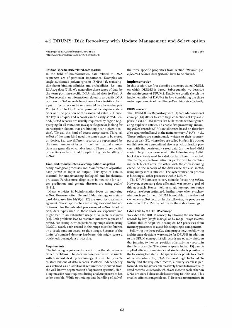
Nettling et al. BMC Bioinformatics 2014, 15:38 Page 2 of 9http://www.biomedcentral.com/1471-2105/15/38

Position-specific DNA related data (psDrd)In the field of bioinformatics, data related to DNAsequences are of particular importance. Examples aresingle nucleotide polymorphisms (SNPs) [4], transcrip-tion factor binding affinities and probabilities [5,6], andRNAseq data [7,8]. We generalize these types of data bythe term position-specific DNA-related data (psDrd). ApsDrd record is an information related to a specific DNAposition. psDrd records have three characteristics. First,a psDrd record R can be represented by a key-value pairR = (K ,V ). The key K is composed of the sequence iden-tifier and the position of the associated value V. Hence,the key is unique, and records can be easily sorted. Sec-ond, psDrd records are usually requested by region (e.g.,querying for all mutations in a specific gene or looking fortranscription factors that are binding near a given posi-tion). We call this kind of access range select. Third, allpsDrd of the same kind need the same space to be storedon device, i.e., two different records are represented bythe same number of bytes. In contrast, textual annota-tions are generally of variable length. These three specificproperties can be utilized for optimizing data handling ofpsDrd.

Time- and resource-intensive computations on psDrdMany biological processes and bioinformatics algorithmhave psDrd as input or output. This type of data isessential for understanding biological and biochemicalprocesses. Furthermore, diagnostics in medicine for can-cer prediction and genetic diseases are using psDrd[9-11].Many activities in bioinformatics focus on analyzing

psDrd. However, often file and folder strategy or a stan-dard databases like MySQL [12] are used for data man-agement. These approaches are straightforward but notoptimized for the intended processing of psDrd. In addi-tion, data types used in these tools are expensive andmight lead to an exhaustive usage of valuable resources[13]. Both problems lead to resource-intensive requests ofpsDrd. For example, when performing range selects usingMySQL, nearly each record in the range must be fetchedby a costly random access to the storage. Because of thelimits of standard desktop hardware, this might cause abottleneck during data processing.

RequirementsThe following requirements result from the above men-tioned problems: The data management must be usablewith standard desktop technology. It must be possibleto store billions of data records. Platform independencywas defined as an additional requirement (derived fromthe well-known segmentation of operation systems). Han-dling massive read requests during analytic processes hasto be possible. While optimizing data handling of psDrd,

the three specific properties from section “Position-spe-cific DNA related data (psDrd)” have to be obeyed.

ImplementationIn this section, we first describe a concept called DRUM,on which DRUMS is based. Subsequently, we describethe architecture of DRUMS. Finally, we briefly sketch theimplementation of DRUMS in Java considering the threemain requirements of handling psDrd data sets efficiently.

DRUM conceptThe DRUM (Disk Repository with Update Management)concept [14] allows to store large collections of key-valuepairs (KVs). DRUM allows fast bulk inserts without gener-ating duplicate entries. To enable fast processing, incom-ing psDrd records (K ,V ) are allocated based on their keyK to separate buffers B in the main memory:M(K) → Bi.Those buffers are continuously written to their counter-parts on disk (D), where they are called buckets. If a bucketon disk reaches a predefined size, a synchronisation pro-cess with the persistently saved data (on the hard disk)starts. The process is executed in the following way: A diskbucket is entirely read to a disk cache. There it is sorted.Thereafter, a synchronisation is performed by combin-ing each bucket after the other with the correspondingcache. As the records of the disk cache are also sorted,using mergesort is efficient. The synchronisation processis blocking all other processes within DRUM.The DRUM concept is very suitable for storing psDrd.

However, requesting data efficiently was never a goal ofthis approach. Hence, neither single lookups nor rangeselects have been optimized. Furthermore, when synchro-nisation is performed, DRUM is not able to receive andcache new psDrd records. In the following, we propose anextension of DRUM that addresses these shortcomings.

Extensions by the DRUMS conceptWe extend the DRUMconcept by allowing the selection ofrecords by key (single lookup) or by range (range selects).Within this concept we decoupled I/O-processes frommemory processes to avoid blocking single components.Following the three psDrd data properties, the following

architecture decisions were made for DRUMS in additionto the DRUM concept: 1) All records are equally sized, sothat jumping to the start position of an arbitrary record inthe file is possible. Therefore, a sparse index [15] can beapplied efficiently, making rapid single selects possible bythe following two steps: The sparse index points to a blockof records, where the psDrd of interest might be found. Tofinally find the requested record, a binary search is per-formed. The binary searchmassively benefits from equallysized records. 2) Records, which are close to each other onDNA are stored close on disk according to their keys. Thisenables efficient range selects. 3) Records are organized in

4.2 DRUMS: Disk Repository with Update Management and Select option

63

Page 74

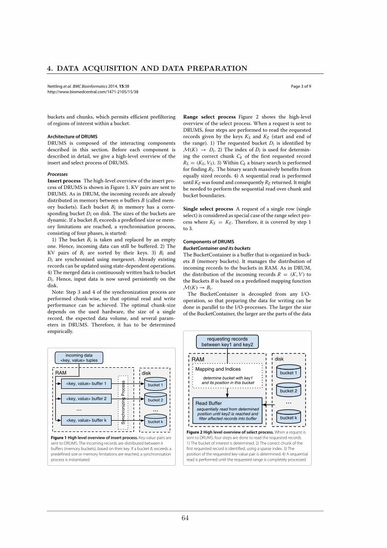
Nettling et al. BMC Bioinformatics 2014, 15:38 Page 3 of 9http://www.biomedcentral.com/1471-2105/15/38

buckets and chunks, which permits efficient prefilteringof regions of interest within a bucket.

Architecture of DRUMSDRUMS is composed of the interacting componentsdescribed in this section. Before each component isdescribed in detail, we give a high-level overview of theinsert and select process of DRUMS.

ProcessesInsert process The high-level overview of the insert pro-cess of DRUMS is shown in Figure 1. KV pairs are sent toDRUMS. As in DRUM, the incoming records are alreadydistributed in memory between n buffers B (called mem-ory buckets). Each bucket Bi in memory has a corre-sponding bucket Di on disk. The sizes of the buckets aredynamic. If a bucket Bi exceeds a predefined size or mem-ory limitations are reached, a synchronisation process,consisting of four phases, is started:1) The bucket Bi is taken and replaced by an empty

one. Hence, incoming data can still be buffered. 2) TheKV pairs of Bi are sorted by their keys. 3) Bi andDi are synchronised using mergesort. Already existingrecords can be updated using state-dependent operations.4) Themerged data is continuously written back to bucketDi. Hence, input data is now saved persistently on thedisk.Note: Step 3 and 4 of the synchronization process are

performed chunk-wise, so that optimal read and writeperformance can be achieved. The optimal chunk-sizedepends on the used hardware, the size of a singlerecord, the expected data volume, and several param-eters in DRUMS. Therefore, it has to be determinedempirically.

incoming data<key, value> tuples

RAM disk

<key, value> buffer 1

<key, value> buffer 2

<key, value> buffer k

...

bucket 1

bucket 2

bucket k

...

Syn

chro

nizi

ng P

roce

ss

Figure 1 High level overview of insert process. Key-value pairs aresent to DRUMS. The incoming records are distributed between kbuffers (memory buckets), based on their key. If a bucket Bi exceeds apredefined size or memory limitations are reached, a synchronisationprocess is instantiated.

Range select process Figure 2 shows the high-leveloverview of the select process. When a request is sent toDRUMS, four steps are performed to read the requestedrecords given by the keys KS and KE (start and end ofthe range). 1) The requested bucket Di is identified byM(K) → Di. 2) The index of Di is used for determin-ing the correct chunk Ck of the first requested recordRS = (KS,VS). 3) Within Ck a binary search is performedfor finding RS. The binary search massively benefits fromequally sized records. 4) A sequential read is performeduntilKE was found and consequently RE returned. It mightbe needed to perform the sequential read over chunk andbucket boundaries.

Single select process A request of a single row (singleselect) is considered as special case of the range select pro-cess where KS = KE . Therefore, it is covered by step 1to 3.

Components of DRUMSBucketContainer and its bucketsThe BucketContainer is a buffer that is organized in buck-ets B (memory buckets). It manages the distribution ofincoming records to the buckets in RAM. As in DRUM,the distribution of the incoming records R = (K ,V ) tothe Buckets B is based on a predefined mapping functionM(K) → Bi.The BucketContainer is decoupled from any I/O-

operation, so that preparing the data for writing can bedone in parallel to the I/O-processes. The larger the sizeof the BucketContainer, the larger are the parts of the data

requesting records between key1 and key2

RAM disk

bucket 1

bucket 2

bucket k

Mapping and Indices

determine bucket with key1 and its position in this bucket

Read Buffersequentially read from determined position until key2 is reached and filter affected records into buffer

...

Figure 2 High level overview of select process.When a request issent to DRUMS, four steps are done to read the requested records.1) The bucket of interest is determined. 2) The correct chunk of thefirst requested record is identified, using a sparse index. 3) Theposition of the requested key-value pair is determined. 4) A sequentialread is performed until the requested range is completely processed.

4. DATA ACQUISITION AND DATA PREPARATION

64

Page 75

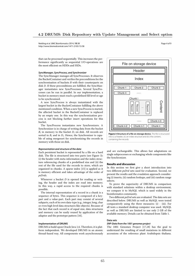
Nettling et al. BMC Bioinformatics 2014, 15:38 Page 4 of 9http://www.biomedcentral.com/1471-2105/15/38

that can be processed sequentially. This increases the per-formance significantly as sequential I/O-operations arethe most efficient on HDDs and SSDs.

SyncManager, SyncProcess, and SynchronizerThe SyncManager manages all SyncProcesses. It observesthe BucketContainer and verifies the preconditions for thesynchronisation of buckets B with their counterparts ondisk D. If these preconditions are fulfilled, the SyncMan-ager instantiates new SyncProcesses. Several SyncPro-cesses can be run in parallel. In our implementation, abucket in memory must reach a predefined fill level or ageto be synchronized.A new SyncProcess is always instantiated with the

largest bucket in the BucketContainer fulfilling the abovementioned condition. When a new SyncProcess is started,the affected bucket in the BucketContainer is replacedby an empty one. In this way the synchronization pro-cess is not blocking further insert operations for thisbucket.The SyncProcess instantiates new Synchronizers. A

Synchronizer is in charge of writing data from the bucketBi in memory to the bucket Di on disk. All records aresorted in Bi and in Di. Hence, the Synchronizer is capa-ble of using mergesort for synchronizing the records inmemory with those on disk.

Representationand structure of the dataEach persistent bucket is represented by a file on a harddisk. The file is structured into two parts (see Figure 3):(i) the header with meta information and the index struc-ture referencing chunks of a predefined size and (ii) therest of the file used for the records to store, which areorganized in chunks. A sparse index [15] is applied as itis memory efficient and takes advantage of the order ofpsDrds.Whenever a bucket D is opened for reading or writ-

ing, the header and the index are read into memory.In this way, a rapid access to the required chunks ispossible.The internal representation of a record in a chunk is a

sequence of bytes. This sequence is composed of a key-part and a value-part. Each part may consist of severalsubparts, each of its own data-type (e.g., integer, long, charor even high level data structures like objects). Because ofthe fact that each record is of equal size, data structuresand memory can be easily reused by application of theadaptor and the prototype pattern [16].

Implementation of DRUMSDRUMS is build upon Oracle Java 1.6. Therefore, it is plat-form independent. We developed DRUMS in an atomicthread-based way. All components work asynchronously

File on storage device

Header

Index

Content

Chunk 1 Chunk 2 Chunk 3

Chunk 4 .....

Chunk n-2 Chunk n-1 Chunk n

Chunk n-3.....

Record

Record

Record

...

Chunk i

Figure 3 Structure of a file on storage device. The file is structuredinto (i.) a header, (ii.) an index structure and (iii.) the content,containing the records.

and are exchangeable. This allows fast adaptations onsingle subprocesses or exchanging whole components likethe Synchronizer.

Results and discussionIn this section we first give a short introduction intotwo different psDrd sets used for evaluation. Second, wepresent the results and the evaulation approach consider-ing (i) inserts, (ii) random lookups, and (iii) random rangeselects.To prove the superiority of DRUMS in comparison

with standard solutions within a desktop environment,we compare it to MySQL which is used widely in thebioinformatics community.Two different psDrd sets are evaluated. The data sets are

described below. DRUMS as well as MySQL were testedcomparatively using the three measures: (i) - (iii). Forall tests a standard desktop computer was used. MySQLas well as DRUMS are limited to use only 2 GB of theavailable memory. Details can be obtained from Table 1.

Data setsSNP-Data from the 1001 genomes projectThe 1001 Genomes Project [17,18] has the goal tounderstand the resulting of small mutations in differentaccessions of the reference plant Arabidopsis thaliana.

4.2 DRUMS: Disk Repository with Update Management and Select option

65

Page 76

Nettling et al. BMC Bioinformatics 2014, 15:38 Page 5 of 9http://www.biomedcentral.com/1471-2105/15/38

Table 1 Test system

Processor Intel Xeon E31225(4 native cores, no hyperthreading)

Memory 8 GB

Operation system Debian 6.0 (Squeeze)

Hard drive Western digital WD10EALX-759, 32 MB cache

The desktop system which was used for the tests. MySQL as well as DRUMS arelimited to use only 2 GB of the available memory.

Each accession mainly consists of five attributes: acces-sion identifier, sequence identifier, position on sequence,source base, and target base. We downloaded filteredquality data of the strains sequenced by the GregorMendel Institute and the Salk institute on 2012-01-15,containing 251 data sets, with 137, 369, 902SNPs. From allfiles, we extracted the data of the following five columns:accession name, chromosome, position on chromosomereference nucleotide, and mutated nucleotide. For the def-initions of the used data types and their configuration(e.g., index properties) used in MySQL and DRUMS seeTable 2.All data are public available at http://1001genomes.org/

datacenter/.

HERV dataHuman endogenous retroviruses (HERVs) have integratedthemselves in the human genome millions of years ago.Because of the high number of existing HERV fragments,they are thought to have a regulatory role. To investigate apossible influence of HERVs, it is needed to locate HERVfragments. Therefore, over 7000 known HERV fragmentswere blasted against the human genome to find newputative HERV-like regions. In the work of KonstantinKruse [19] all regions with an E-value less than 1e − 20were accepted as putative HERV-like region. This lead to802, 710, 938 single records, stored in 20 files with tab-separated data field, with a total size of 50 GB. From thesefiles we used the following seven columns: query id, sub-ject id, query start, query end, subject start, subject end,and E-value. For the definitions of the used data types andtheir configuration (e.g., index properties) used inMySQLand DRUMS see Table 3.

Table 2 Data types used for SNP data

Column MySQL properties DRUMS properties

Accession name TINY INT, primary key 1 byte, key part 1

Chromosome SMALL INT, primary key 2 byte, key part 2

Position on chromosome INT, primary key 4 byte, key part 3

Reference nucleotide VARCHAR 1 byte, value part 1

Mutated nucleotide VARCHAR 1 byte, value part 2

Used data types in MySQL and DRUMS for SNP data. All columns being part ofthe primary key are indexed.

Insert performanceDRUMS must be able to store hundreds of millions ofrecords. Because of this, it is needed to evaluate the insertperformance.To estimate the insert performance, we measure the

time for inserting 106 records. We obtain 140 time mea-surements points in case of SNP-Data and 800 for HERVdata. Figures 4a and 4b show the insert performance ofDRUMS (blue) and MySQL (green). Despite using bulk-requests for inserting the data, it was impossible to insertall 800 million HERV records into the MySQL instance.MySQL inserts about 200 million records in the firstweek, but Figure 4b shows that the insert performance hasdropped to 300 records per second after one week. Theinsert performance of DRUMS also decreases, but it wasable to insert the whole data set within 4.53 hours. At theend of the test, DRUMS was still able to perform morethan 20000 inserts per second.Figure 4a and 4b show that DRUMS has a better insert

performance than MySQL on both test datasets. Theinsert performance of MySQL and of DRUMS decreaseswith the number of records already inserted. Regard-ing MySQL one possible explanation is the continuousreorganistation and rewriting of the index.The insert performance of DRUMS decreases slowly

in comparison to MySQL. The reason for this is thedecreasing ratio of read- to write-accesses with eachround of synchronisation. With other words, DRUMSmust read more and more records per new record towrite with the growing amount of data already storedon disk. However, DRUMS still inserts more than 20000records per second at the end of the insert test forHERV data, corresponding to approximately 400 kB persecond.

Performance on random lookupsFrom the view of bioinformatics, single lookups makeno sense in both experiments. However, the performanceof single-lookups is a significant indicator for the over-all performance and the suitability of the implementa-tion of a tool for handling data sets. Moreover, the testmay show how close the measured performance to thetheoretical hardware limits of the used standard desk-top hardware is. Considering the test environment, itis assumed that a random access would take approxi-mately 20 ms. Hence, if no other disk accesses are done,it would be theoretically possible to read 50 records persecond.Figures 5a and 5b show the performance of MySQL

and DRUMS, when performing random lookups. Again,DRUMS performs better than MySQL in case of han-dling our two data sets. Figure 5a implies that DRUMS isable to do 160 times more random lookups than theoret-ically possible, when accessing SNP data. In comparison,

4. DATA ACQUISITION AND DATA PREPARATION

66

Page 77

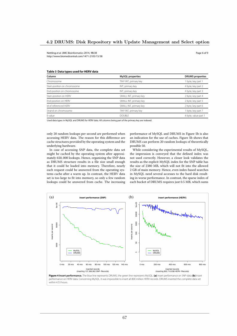
Nettling et al. BMC Bioinformatics 2014, 15:38 Page 6 of 9http://www.biomedcentral.com/1471-2105/15/38

Table 3 Data types used for HERV data

Column MySQL properties DRUMS properties

Chromosome TINY INT, primary key 1 byte, key part 1

Start-position on chromosome INT, primary key 4 byte, key part 2

End-position on chromosome INT, primary key 4 byte, key part 3

Start-position on HERV SMALL INT, primary key 2 byte, key part 4

End-position on HERV SMALL INT, primary key 2 byte, key part 5

Id of referenced HERV SMALL INT, primary key 2 byte, key part 6

Strand on chromosome TINY INT, primary key 1 byte, key part 7

E-value DOUBLE 4 byte, value part 1

Used data types in MySQL and DRUMS for HERV data. All columns being part of the primary key are indexed.

only 20 random lookups per second are performed whenaccessing HERV data. The reason for this difference arecache structures provided by the operating system and theunderlying hardware.In case of accessing SNP data, the complete data set

might be cached by the operating system after approxi-mately 650, 000 lookups. Hence, organizing the SNP dataas DRUMS structure results in a file size small enoughthat it could be loaded into memory. Therefore, nearlyeach request could be answered from the operating sys-tems cache after a warm up. In contrast, the HERV dataset is too large to fit into memory, so only a few randomlookups could be answered from cache. The increasing

performance of MySQL and DRUMS in Figure 5b is alsoan indication for the use of caches. Figure 5b shows thatDRUMS can perform 20 random lookups of theoreticallypossible 50.While considering the experimental results of MySQL,

the impression is conveyed that the defined index wasnot used correctly. However, a closer look validates theresults as the explicit MySQL index for the SNP table hasthe size of 2380 MB, which will not fit into the allowed2 GB of main memory. Hence, even index-based searchesin MySQL need several accesses to the hard disk result-ing in worse performance. In contrast, the sparse index ofeach bucket of DRUMS requires just 0.5 MB, which sums

insert performance (SNP)

(inserting 137.369.902 SNP−Records)inserted records

inse

rts

per

seco

nd

0 mio 20 mio 40 mio 60 mio 80 mio 100 mio 120 mio 140 mio

5000

5000

05e

+05

MySQLDRUMS

(a) insert performance (HERV)

(inserting 802.710.938 HERV−Records)inserted records

inse

rts

per

seco

nd

0 mio 200 mio 400 mio 600 mio 800 mio

550

500

5000

5000

05e

+05

MySQLDRUMS

(b)

Figure 4 Insert performance. The blue line represents DRUMS, the green line represents MySQL. (a) Insert performance on SNP-data (b) Insertperformance on HERV data. Concerning MySQL, it was impossible to insert all 800 million HERV records. DRUMS inserted the complete data setwithin 4.53 hours.

4.2 DRUMS: Disk Repository with Update Management and Select option

67

Page 78

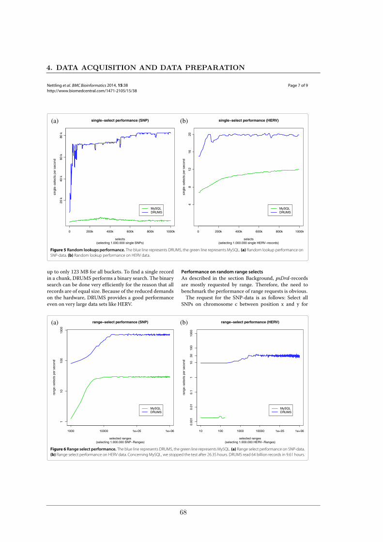
Nettling et al. BMC Bioinformatics 2014, 15:38 Page 7 of 9http://www.biomedcentral.com/1471-2105/15/38

single−select performance (SNP)

(selecting 1.000.000 single SNPs)selects

sing

le−

sele

cts

per

seco

nd

0 200k 400k 600k 800k 1000k

20 k

40 k

60 k

80 k

MySQLDRUMS

(a) single−select performance (HERV)

(selecting 1.000.000 single HERV−records)selects

sing

le−

sele

cts

per

seco

nd

0 200k 400k 600k 800k 1000k

48

1216

20

MySQLDRUMS

(b)

Figure 5 Random lookups performance. The blue line represents DRUMS, the green line represents MySQL. (a) Random lookup performance onSNP-data. (b) Random lookup performance on HERV data.

up to only 123 MB for all buckets. To find a single recordin a chunk, DRUMS performs a binary search. The binarysearch can be done very efficiently for the reason that allrecords are of equal size. Because of the reduced demandson the hardware, DRUMS provides a good performanceeven on very large data sets like HERV.

Performance on random range selectsAs described in the section Background, psDrd-recordsare mostly requested by range. Therefore, the need tobenchmark the performance of range requests is obvious.The request for the SNP-data is as follows: Select all

SNPs on chromosome c between position x and y for

range−select performance (SNP)

(selecting 1.000.000 SNP−Ranges)selected ranges

rang

e−se

lect

s pe

r se

cond

1000 10000 1e+05 1e+06

110

100

1000

MySQLDRUMS

(a) range−select performance (HERV)

(selecting 1.000.000 HERV−Ranges)selected ranges

rang

e−se

lect

s pe

r se

cond

10 100 1000 10000 1e+05 1e+06

0.00

10.

010.

11

1030

100

1000

MySQLDRUMS

(b)

Figure 6 Range select performance. The blue line represents DRUMS, the green line represents MySQL. (a) Range select performance on SNP-data.(b) Range select performance on HERV data. Concerning MySQL, we stopped the test after 26.35 hours. DRUMS read 64 billion records in 9.61 hours.

4. DATA ACQUISITION AND DATA PREPARATION

68

Page 79

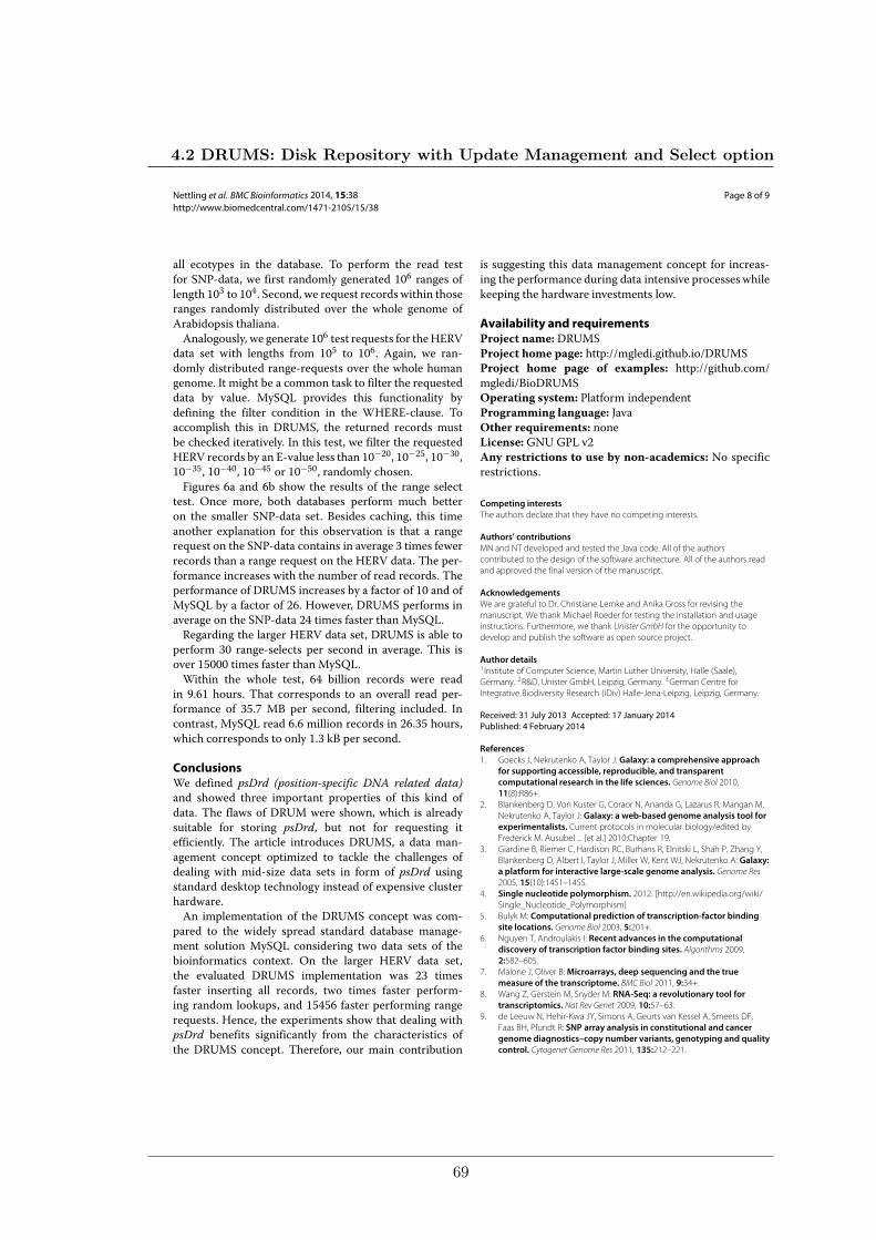
Nettling et al. BMC Bioinformatics 2014, 15:38 Page 8 of 9http://www.biomedcentral.com/1471-2105/15/38

all ecotypes in the database. To perform the read testfor SNP-data, we first randomly generated 106 ranges oflength 103 to 104. Second, we request records within thoseranges randomly distributed over the whole genome ofArabidopsis thaliana.Analogously, we generate 106 test requests for theHERV

data set with lengths from 105 to 106. Again, we ran-domly distributed range-requests over the whole humangenome. It might be a common task to filter the requesteddata by value. MySQL provides this functionality bydefining the filter condition in the WHERE-clause. Toaccomplish this in DRUMS, the returned records mustbe checked iteratively. In this test, we filter the requestedHERV records by an E-value less than 10−20, 10−25, 10−30,10−35, 10−40, 10−45 or 10−50, randomly chosen.Figures 6a and 6b show the results of the range select

test. Once more, both databases perform much betteron the smaller SNP-data set. Besides caching, this timeanother explanation for this observation is that a rangerequest on the SNP-data contains in average 3 times fewerrecords than a range request on the HERV data. The per-formance increases with the number of read records. Theperformance of DRUMS increases by a factor of 10 and ofMySQL by a factor of 26. However, DRUMS performs inaverage on the SNP-data 24 times faster than MySQL.Regarding the larger HERV data set, DRUMS is able to

perform 30 range-selects per second in average. This isover 15000 times faster than MySQL.Within the whole test, 64 billion records were read

in 9.61 hours. That corresponds to an overall read per-formance of 35.7 MB per second, filtering included. Incontrast, MySQL read 6.6 million records in 26.35 hours,which corresponds to only 1.3 kB per second.

ConclusionsWe defined psDrd (position-specific DNA related data)and showed three important properties of this kind ofdata. The flaws of DRUM were shown, which is alreadysuitable for storing psDrd, but not for requesting itefficiently. The article introduces DRUMS, a data man-agement concept optimized to tackle the challenges ofdealing with mid-size data sets in form of psDrd usingstandard desktop technology instead of expensive clusterhardware.An implementation of the DRUMS concept was com-

pared to the widely spread standard database manage-ment solution MySQL considering two data sets of thebioinformatics context. On the larger HERV data set,the evaluated DRUMS implementation was 23 timesfaster inserting all records, two times faster perform-ing random lookups, and 15456 faster performing rangerequests. Hence, the experiments show that dealing withpsDrd benefits significantly from the characteristics ofthe DRUMS concept. Therefore, our main contribution

is suggesting this data management concept for increas-ing the performance during data intensive processes whilekeeping the hardware investments low.

Availability and requirementsProject name: DRUMSProject home page: http://mgledi.github.io/DRUMSProject home page of examples: http://github.com/mgledi/BioDRUMSOperating system: Platform independentProgramming language: JavaOther requirements: noneLicense: GNU GPL v2Any restrictions to use by non-academics: No specificrestrictions.

Competing interestsThe authors declare that they have no competing interests.

Authors’ contributionsMN and NT developed and tested the Java code. All of the authorscontributed to the design of the software architecture. All of the authors readand approved the final version of the manuscript.

AcknowledgementsWe are grateful to Dr. Christiane Lemke and Anika Gross for revising themanuscript. We thank Michael Roeder for testing the installation and usageinstructions. Furthermore, we thank Unister GmbH for the opportunity todevelop and publish the software as open source project.

Author details1Institute of Computer Science, Martin Luther University, Halle (Saale),Germany. 2R&D, Unister GmbH, Leipzig, Germany. 3German Centre forIntegrative Biodiversity Research (iDiv) Halle-Jena-Leipzig, Leipzig, Germany.

Received: 31 July 2013 Accepted: 17 January 2014Published: 4 February 2014

References1. Goecks J, Nekrutenko A, Taylor J: Galaxy: a comprehensive approach

for supporting accessible, reproducible, and transparentcomputational research in the life sciences. Genome Biol 2010,11(8):R86+.

2. Blankenberg D, Von Kuster G, Coraor N, Ananda G, Lazarus R, Mangan M,Nekrutenko A, Taylor J: Galaxy: a web-based genome analysis tool forexperimentalists. Current protocols in molecular biology/edited byFrederick M. Ausubel ... [et al.] 2010:Chapter 19.

3. Giardine B, Riemer C, Hardison RC, Burhans R, Elnitski L, Shah P, Zhang Y,Blankenberg D, Albert I, Taylor J, Miller W, Kent WJ, Nekrutenko A: Galaxy:a platform for interactive large-scale genome analysis. Genome Res2005, 15(10):1451–1455.

4. Single nucleotide polymorphism. 2012. [http://en.wikipedia.org/wiki/Single_Nucleotide_Polymorphism]

5. Bulyk M: Computational prediction of transcription-factor bindingsite locations. Genome Biol 2003, 5:201+.

6. Nguyen T, Androulakis I: Recent advances in the computationaldiscovery of transcription factor binding sites. Algorithms 2009,2:582–605.

7. Malone J, Oliver B:Microarrays, deep sequencing and the truemeasure of the transcriptome. BMC Biol 2011, 9:34+.

8. Wang Z, Gerstein M, Snyder M: RNA-Seq: a revolutionary tool fortranscriptomics. Nat Rev Genet 2009, 10:57–63.

9. de Leeuw N, Hehir-Kwa JY, Simons A, Geurts van Kessel A, Smeets DF,Faas BH, Pfundt R: SNP array analysis in constitutional and cancergenome diagnostics–copy number variants, genotyping and qualitycontrol. Cytogenet Genome Res 2011, 135:212–221.

4.2 DRUMS: Disk Repository with Update Management and Select option

69

Page 80

Nettling et al. BMC Bioinformatics 2014, 15:38 Page 9 of 9http://www.biomedcentral.com/1471-2105/15/38

10. Kihara D, Yang YDD, Hawkins T: Bioinformatics resources for cancerresearch with an emphasis on gene function and structureprediction tools. Cancer Inform 2006, 2:25–35.

11. Roukos DH: Next-Generation Sequencing &Molecular Diagnostics. London:Future Medicine Ltd; 2013.

12. MySQL classic edition. 2012. [http://www.mysql.com/products/classic/]13. Common wrong data types. 2012. [http://code.openark.org/blog/

mysql/common-data-types-errors-compilation]14. Lee HT, Leonard D, Wang X, Loguinov D: IRLbot: scaling to 6 billion

pages and beyond. In Proceedings of the 17th international conference onWorld Wide Web, WWW ’08.New York, NY, USA: ACM; 2008:427–436.

15. Database index - sparse index. 2012. [http://en.wikipedia.org/wiki/Database_index#Sparse_index]

16. Gamma E, Helm R, Johnson R, Vlissides J: Design patterns: elements ofreusable object-oriented software. Boston, MA, USA: Addison-WesleyLongman Publishing Co., Inc.; 1995.

17. Schneeberger K, Ossowski S, Ott F, Klein JD, Wang X, Lanz C, Smith LM,Cao J, Fitz J, Warthmann N, Henz SR, Huson DH, Weigel D:Reference-guided assembly of four diverse Arabidopsis thalianagenomes. Proc Nat Acad Sci USA 2011, 108(25):10249–10254.

18. Cao J, Schneeberger K, Ossowski S, Günther T, Bender S, Fitz J, Koenig D,Lanz C, Stegle O, Lippert C, Wang X, Ott F, Müller J, Alonso-Blanco C,Borgwardt K, Schmid KJ, Weigel D:Whole-genome sequencing ofmultiple Arabidopsis thaliana populations. Nat Genet 2011,43(10):956–963.

19. Kruse K: Analysis of gene expression in correlation to endogenousretroviruses.Martin Luther University, Halle (Saale) Germany 2011.[Bachelor Thesis]

doi:10.1186/1471-2105-15-38Cite this article as: Nettling et al.: DRUMS: Disk Repository with UpdateManagement and Select option for high throughput sequencing data. BMCBioinformatics 2014 15:38.

Submit your next manuscript to BioMed Centraland take full advantage of:

• Convenient online submission

• Thorough peer review

• No space constraints or color figure charges

• Immediate publication on acceptance

• Inclusion in PubMed, CAS, Scopus and Google Scholar

• Research which is freely available for redistribution

Submit your manuscript at www.biomedcentral.com/submit

4. DATA ACQUISITION AND DATA PREPARATION

70

Page 81

5 Predicting transcription factor binding sitesusing Phylogenetic Footprinting

5.1 Detecting and correcting the binding-affinity bias in ChIP-Seq data using inter-species information

M Nettling, H Treutler, J Cerquides, I Grosse. 2016. Detecting and correcting thebinding-affinity bias in ChIP-Seq data using inter-species information. BMC Genomics17:1. doi:10.1186/s12864-016-2682-6

71

Page 82

Nettling et al. BMC Genomics (2016) 17:347 DOI 10.1186/s12864-016-2682-6

METHODOLOGY ARTICLE Open Access

Detecting and correcting thebinding-affinity bias in ChIP-seq data usinginter-species informationMartin Nettling1*, Hendrik Treutler2, Jesus Cerquides3 and Ivo Grosse1,4

Abstract

Background: Transcriptional gene regulation is a fundamental process in nature, and the experimental andcomputational investigation of DNA binding motifs and their binding sites is a prerequisite for elucidating this process.ChIP-seq has become the major technology to uncover genomic regions containing those binding sites, but motifspredicted by traditional computational approaches using these data are distorted by a ubiquitous binding-affinitybias. Here, we present an approach for detecting and correcting this bias using inter-species information.

Results: We find that the binding-affinity bias caused by the ChIP-seq experiment in the reference species is strongerthan the indirect binding-affinity bias in orthologous regions from phylogenetically related species. We use thisdifference to develop a phylogenetic footprinting model that is capable of detecting and correcting thebinding-affinity bias. We find that this model improves motif prediction and that the corrected motifs are typicallysofter than those predicted by traditional approaches.

Conclusions: These findings indicate that motifs published in databases and in the literature are artificiallysharpened compared to the native motifs. These findings also indicate that our current understanding oftranscriptional gene regulation might be blurred, but that it is possible to advance this understanding by taking intoaccount inter-species information available today and even more in the future.

Keywords: Binding-affinity bias, ChIP-seq, Phylogenetic footprinting, Evolution, Transcription factor binding sites,Gene regulation

BackgroundPredicting transcription factor binding sites and theirmotifs is essential for understanding transcriptional generegulation and thus of importance in almost all areasof modern biology, medicine, and biodiversity research[1, 2]. Countless approaches exist for predicting motifsfrom these genomic regions [3–6], but predicting motifsfrom ChIP-seq data and similar experimental data is ham-pered by the contamination with false positive genomicregions as well as the enrichment of high-affinity bindingsites [7–9].

*Correspondence: [email protected] of Computer Science, Martin Luther University, Halle (Saale),GermanyFull list of author information is available at the end of the article

The contamination with false positive genomic regionsis caused by at least three reasons. First, the transcrip-tion factor or other DNA binding protein pulled down byimmunoprecipitation may not bind directly to the bindingsite [10]. Second, ChIP-seq target regions may not con-tain a binding site due to experimental settings such assequencing depth or DNA fragment length [11, 12]. Third,false positive regions may be predicted in the subse-quent ChIP-seq data analysis due to never perfect analysispipelines and too low signal cutoff thresholds [8]. Thesethree effects may lead to the selection of false positiveChIP-seq regions that do not contain at least one bindingsite.The enrichment of high-affinity binding sites is caused

by at least two reasons. First, most antibodies have a pref-erence of binding high-affinity binding sites with a higherprobability than low-affinity binding sites, causing the set

© 2016 Nettling et al. Open Access This article is distributed under the terms of the Creative Commons Attribution 4.0International License (http://creativecommons.org/licenses/by/4.0/), which permits unrestricted use, distribution, andreproduction in any medium, provided you give appropriate credit to the original author(s) and the source, provide a link to theCreative Commons license, and indicate if changes were made. The Creative Commons Public Domain Dedication waiver(http://creativecommons.org/publicdomain/zero/1.0/) applies to the data made available in this article, unless otherwise stated.

5. PREDICTING TRANSCRIPTION FACTOR BINDING SITES USINGPHYLOGENETIC FOOTPRINTING

72

Page 83

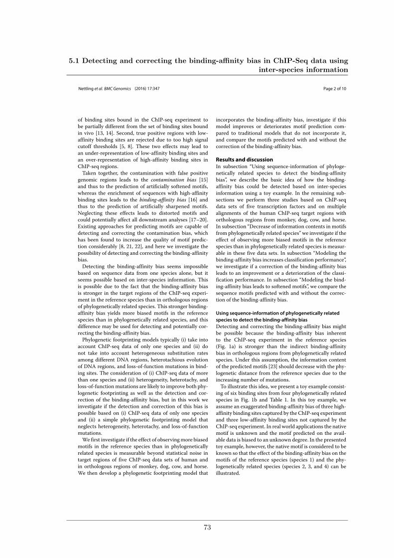
Nettling et al. BMC Genomics (2016) 17:347 Page 2 of 10

of binding sites bound in the ChIP-seq experiment tobe partially different from the set of binding sites boundin vivo [13, 14]. Second, true positive regions with low-affinity binding sites are rejected due to too high signalcutoff thresholds [5, 8]. These two effects may lead toan under-representation of low-affinity binding sites andan over-representation of high-affinity binding sites inChIP-seq regions.Taken together, the contamination with false positive

genomic regions leads to the contamination bias [15]and thus to the prediction of artificially softened motifs,whereas the enrichment of sequences with high-affinitybinding sites leads to the binding-affinity bias [16] andthus to the prediction of artificially sharpened motifs.Neglecting these effects leads to distorted motifs andcould potentially affect all downstream analyses [17–20].Existing approaches for predicting motifs are capable ofdetecting and correcting the contamination bias, whichhas been found to increase the quality of motif predic-tion considerably [8, 21, 22], and here we investigate thepossibility of detecting and correcting the binding-affinitybias.Detecting the binding-affinity bias seems impossible

based on sequence data from one species alone, but itseems possible based on inter-species information. Thisis possible due to the fact that the binding-affinity biasis stronger in the target regions of the ChIP-seq experi-ment in the reference species than in orthologous regionsof phylogenetically related species. This stronger binding-affinity bias yields more biased motifs in the referencespecies than in phylogenetically related species, and thisdifference may be used for detecting and potentially cor-recting the binding-affinity bias.Phylogenetic footprinting models typically (i) take into

account ChIP-seq data of only one species and (ii) donot take into account heterogeneous substitution ratesamong different DNA regions, heterotachious evolutionof DNA regions, and loss-of-function mutations in bind-ing sites. The consideration of (i) ChIP-seq data of morethan one species and (ii) heterogeneity, heterotachy, andloss-of-functionmutations are likely to improve both phy-logenetic footprinting as well as the detection and cor-rection of the binding-affinity bias, but in this work weinvestigate if the detection and correction of this bias ispossible based on (i) ChIP-seq data of only one speciesand (ii) a simple phylogenetic footprinting model thatneglects heterogeneity, heterotachy, and loss-of-functionmutations.We first investigate if the effect of observingmore biased

motifs in the reference species than in phylogeneticallyrelated species is measurable beyond statistical noise intarget regions of five ChIP-seq data sets of human andin orthologous regions of monkey, dog, cow, and horse.We then develop a phylogenetic footprinting model that

incorporates the binding-affinity bias, investigate if thismodel improves or deteriorates motif prediction com-pared to traditional models that do not incorporate it,and compare the motifs predicted with and without thecorrection of the binding-affinity bias.

Results and discussionIn subsection “Using sequence-information of phyloge-netically related species to detect the binding-affinitybias”, we describe the basic idea of how the binding-affinity bias could be detected based on inter-speciesinformation using a toy example. In the remaining sub-sections we perform three studies based on ChIP-seqdata sets of five transcription factors and on multiplealignments of the human ChIP-seq target regions withorthologous regions from monkey, dog, cow, and horse.In subsection “Decrease of information contents in motifsfrom phylogenetically related species” we investigate if theeffect of observing more biased motifs in the referencespecies than in phylogenetically related species is measur-able in these five data sets. In subsection “Modeling thebinding-affinity bias increases classification performance”,we investigate if a correction of the binding-affinity biasleads to an improvement or a deterioration of the classi-fication performance. In subsection “Modeling the bind-ing-affinity bias leads to softened motifs”, we compare thesequence motifs predicted with and without the correc-tion of the binding-affinity bias.

Using sequence-information of phylogenetically relatedspecies to detect the binding-affinity biasDetecting and correcting the binding-affinity bias mightbe possible because the binding-affinity bias inherentto the ChIP-seq experiment in the reference species(Fig. 1a) is stronger than the indirect binding-affinitybias in orthologous regions from phylogenetically relatedspecies. Under this assumption, the information contentof the predicted motifs [23] should decrease with the phy-logenetic distance from the reference species due to theincreasing number of mutations.To illustrate this idea, we present a toy example consist-

ing of six binding sites from four phylogenetically relatedspecies in Fig. 1b and Table 1. In this toy example, weassume an exaggerated binding-affinity bias of three high-affinity binding sites captured by the ChIP-seq experimentand three low-affinity binding sites not captured by theChIP-seq experiment. In real world applications the nativemotif is unknown and the motif predicted on the avail-able data is biased to an unknown degree. In the presentedtoy example, however, the native motif is considered to beknown so that the effect of the binding-affinity bias on themotifs of the reference species (species 1) and the phy-logenetically related species (species 2, 3, and 4) can beillustrated.

5.1 Detecting and correcting the binding-affinity bias in ChIP-Seq data usinginter-species information

73

Page 84

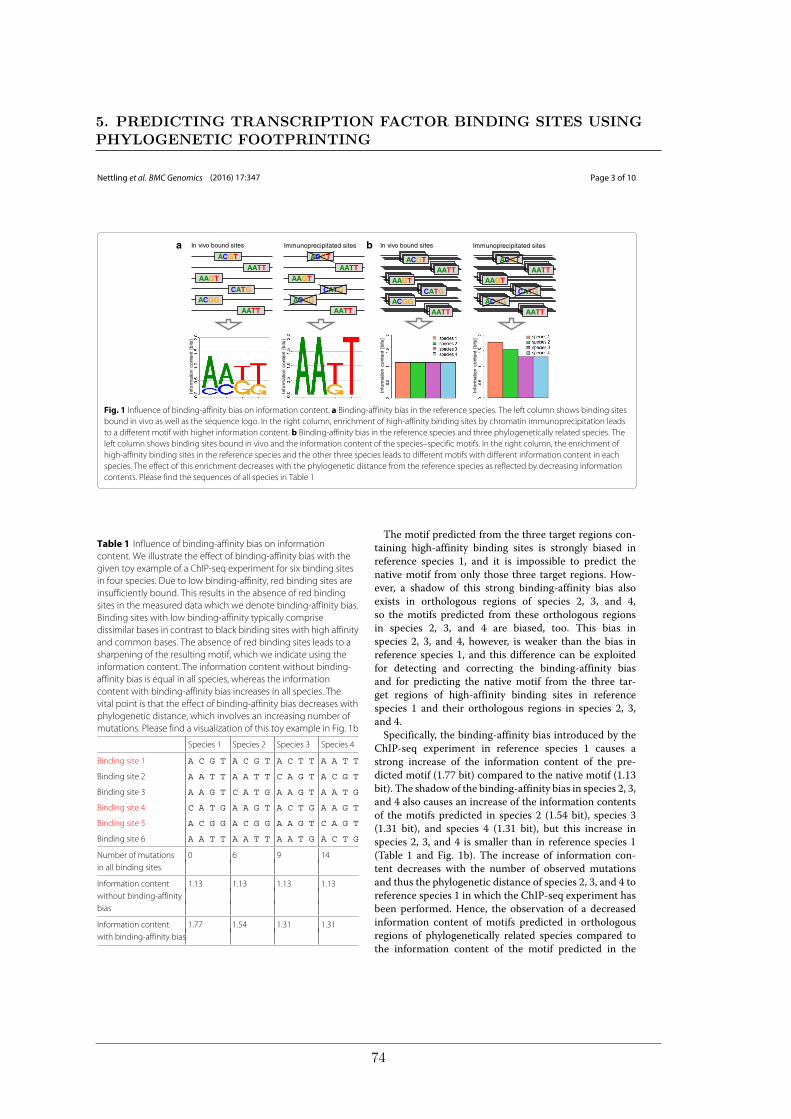
Nettling et al. BMC Genomics (2016) 17:347 Page 3 of 10

ACGT

AATT

AAGT

CATGACGG

AATT

ACGT

AATT

AAGT

CATGACGG

AATT

In vivo bound sites Immunoprecipitated sites

Info

rmat

ion

cont

ent

[bits

]

Info

rmat

ion

cont

ent

[ bits

]

ACGTAATT

AAGT

CATGACGG

AATT

AATTAATTAATT

AATTAATTAATT

ACGGACGGACGG

CATGCATGCATG

AAGTAAGTAAGT

ACGTACGTACGT ACGTAATT

AAGT

CATGACGG

AATT

AATTAATTAATT

AATTAATTAATT

ACGGACGGACGG

CATGCATGCATG

AAGTAAGTAAGT

ACGTACGTACGT

Info

rmat

ion

cont

ent

[bits

]

Info

rmat

ion

cont

ent

[bits

]

In vivo bound sites Immunoprecipitated sitesba

Fig. 1 Influence of binding-affinity bias on information content. a Binding-affinity bias in the reference species. The left column shows binding sitesbound in vivo as well as the sequence logo. In the right column, enrichment of high-affinity binding sites by chromatin immunoprecipitation leadsto a different motif with higher information content. b Binding-affinity bias in the reference species and three phylogenetically related species. Theleft column shows binding sites bound in vivo and the information content of the species–specific motifs. In the right column, the enrichment ofhigh-affinity binding sites in the reference species and the other three species leads to different motifs with different information content in eachspecies. The effect of this enrichment decreases with the phylogenetic distance from the reference species as reflected by decreasing informationcontents. Please find the sequences of all species in Table 1

Table 1 Influence of binding-affinity bias on informationcontent. We illustrate the effect of binding-affinity bias with thegiven toy example of a ChIP-seq experiment for six binding sitesin four species. Due to low binding-affinity, red binding sites areinsufficiently bound. This results in the absence of red bindingsites in the measured data which we denote binding-affinity bias.Binding sites with low binding-affinity typically comprisedissimilar bases in contrast to black binding sites with high affinityand common bases. The absence of red binding sites leads to asharpening of the resulting motif, which we indicate using theinformation content. The information content without binding-affinity bias is equal in all species, whereas the informationcontent with binding-affinity bias increases in all species. Thevital point is that the effect of binding-affinity bias decreases withphylogenetic distance, which involves an increasing number ofmutations. Please find a visualization of this toy example in Fig. 1b

Species 1 Species 2 Species 3 Species 4

Binding site 1 A C G T A C G T A C T T A A T T

Binding site 2 A A T T A A T T C A G T A C G T

Binding site 3 A A G T C A T G A A G T A A T G

Binding site 4 C A T G A A G T A C T G A A G T

Binding site 5 A C G G A C G G A A G T C A G T

Binding site 6 A A T T A A T T A A T G A C T G

Number of mutations 0 6 9 14in all binding sites

Information content 1.13 1.13 1.13 1.13without binding-affinitybias

Information content 1.77 1.54 1.31 1.31with binding-affinity bias

The motif predicted from the three target regions con-taining high-affinity binding sites is strongly biased inreference species 1, and it is impossible to predict thenative motif from only those three target regions. How-ever, a shadow of this strong binding-affinity bias alsoexists in orthologous regions of species 2, 3, and 4,so the motifs predicted from these orthologous regionsin species 2, 3, and 4 are biased, too. This bias inspecies 2, 3, and 4, however, is weaker than the bias inreference species 1, and this difference can be exploitedfor detecting and correcting the binding-affinity biasand for predicting the native motif from the three tar-get regions of high-affinity binding sites in referencespecies 1 and their orthologous regions in species 2, 3,and 4.Specifically, the binding-affinity bias introduced by the

ChIP-seq experiment in reference species 1 causes astrong increase of the information content of the pre-dicted motif (1.77 bit) compared to the native motif (1.13bit). The shadow of the binding-affinity bias in species 2, 3,and 4 also causes an increase of the information contentsof the motifs predicted in species 2 (1.54 bit), species 3(1.31 bit), and species 4 (1.31 bit), but this increase inspecies 2, 3, and 4 is smaller than in reference species 1(Table 1 and Fig. 1b). The increase of information con-tent decreases with the number of observed mutationsand thus the phylogenetic distance of species 2, 3, and 4 toreference species 1 in which the ChIP-seq experiment hasbeen performed. Hence, the observation of a decreasedinformation content of motifs predicted in orthologousregions of phylogenetically related species compared tothe information content of the motif predicted in the

5. PREDICTING TRANSCRIPTION FACTOR BINDING SITES USINGPHYLOGENETIC FOOTPRINTING

74

Page 85

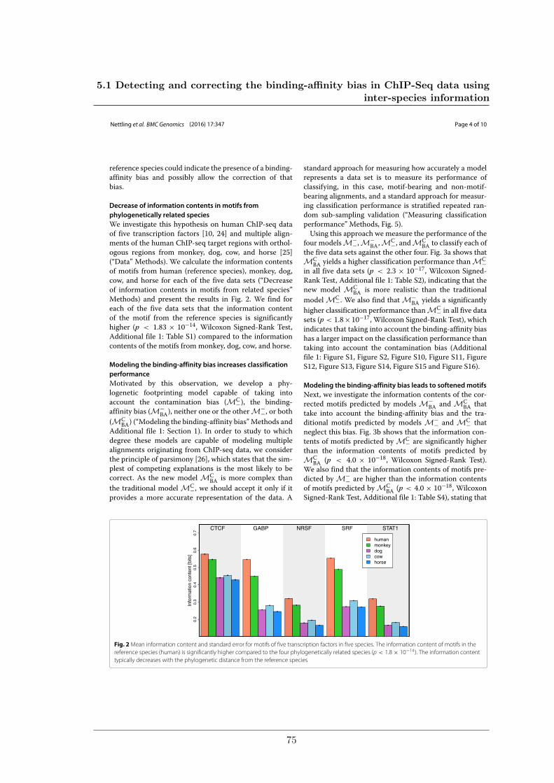
Nettling et al. BMC Genomics (2016) 17:347 Page 4 of 10

reference species could indicate the presence of a binding-affinity bias and possibly allow the correction of thatbias.

Decrease of information contents in motifs fromphylogenetically related speciesWe investigate this hypothesis on human ChIP-seq dataof five transcription factors [10, 24] and multiple align-ments of the human ChIP-seq target regions with orthol-ogous regions from monkey, dog, cow, and horse [25](“Data” Methods). We calculate the information contentsof motifs from human (reference species), monkey, dog,cow, and horse for each of the five data sets (“Decreaseof information contents in motifs from related species”Methods) and present the results in Fig. 2. We find foreach of the five data sets that the information contentof the motif from the reference species is significantlyhigher (p < 1.83 × 10−14, Wilcoxon Signed-Rank Test,Additional file 1: Table S1) compared to the informationcontents of the motifs from monkey, dog, cow, and horse.

Modeling the binding-affinity bias increases classificationperformanceMotivated by this observation, we develop a phy-logenetic footprinting model capable of taking intoaccount the contamination bias (MC−), the binding-affinity bias (M−

BA), neither one or the otherM−−, or both

(MCBA) (“Modeling the binding-affinity bias”Methods and

Additional file 1: Section 1). In order to study to whichdegree these models are capable of modeling multiplealignments originating from ChIP-seq data, we considerthe principle of parsimony [26], which states that the sim-plest of competing explanations is the most likely to becorrect. As the new model MC

BA is more complex thanthe traditional model MC−, we should accept it only if itprovides a more accurate representation of the data. A

standard approach for measuring how accurately a modelrepresents a data set is to measure its performance ofclassifying, in this case, motif-bearing and non-motif-bearing alignments, and a standard approach for measur-ing classification performance is stratified repeated ran-dom sub-sampling validation (“Measuring classificationperformance” Methods, Fig. 5).Using this approach we measure the performance of the

four modelsM−−,M−BA,MC−, andMC

BA to classify each ofthe five data sets against the other four. Fig. 3a shows thatMC

BA yields a higher classification performance thanMC−in all five data sets (p < 2.3 × 10−17, Wilcoxon Signed-Rank Test, Additional file 1: Table S2), indicating that thenew model MC

BA is more realistic than the traditionalmodel MC−. We also find that M−

BA yields a significantlyhigher classification performance thanMC− in all five datasets (p < 1.8×10−17, Wilcoxon Signed-Rank Test), whichindicates that taking into account the binding-affinity biashas a larger impact on the classification performance thantaking into account the contamination bias (Additionalfile 1: Figure S1, Figure S2, Figure S10, Figure S11, FigureS12, Figure S13, Figure S14, Figure S15 and Figure S16).

Modeling the binding-affinity bias leads to softenedmotifsNext, we investigate the information contents of the cor-rected motifs predicted by models M−

BA and MCBA that

take into account the binding-affinity bias and the tra-ditional motifs predicted by models M−− and MC− thatneglect this bias. Fig. 3b shows that the information con-tents of motifs predicted by MC− are significantly higherthan the information contents of motifs predicted byMC

BA (p < 4.0 × 10−18, Wilcoxon Signed-Rank Test).We also find that the information contents of motifs pre-dicted by M−− are higher than the information contentsof motifs predicted by MC

BA (p < 4.0 × 10−18, WilcoxonSigned-Rank Test, Additional file 1: Table S4), stating that

CTCF GABP NRSF SRF STAT1

Info

rmat

ion

cont

ent [

bits

]0.

20.

30.

40.

50.

60.

7

humanmonkeydogcowhorse

Fig. 2Mean information content and standard error for motifs of five transcription factors in five species. The information content of motifs in thereference species (human) is significantly higher compared to the four phylogenetically related species (p < 1.8 × 10−14). The information contenttypically decreases with the phylogenetic distance from the reference species

5.1 Detecting and correcting the binding-affinity bias in ChIP-Seq data usinginter-species information

75

Page 86

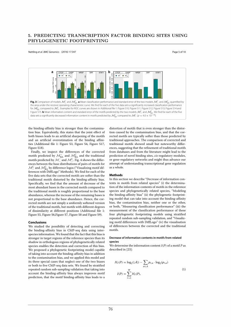
Nettling et al. BMC Genomics (2016) 17:347 Page 5 of 10

CTCF GABP NRSF SRF STAT1

Are

a un

der

RO

C c

urve

0.84

0.85

0.86

0.79

0.85

0.86

0.87

0.6

0.62

0.64

0.66

0.68

0.79

0.8

M –C M BA

C

CTCF GABP NRSF SRF STAT1

Info

rmat

ion

cont

ent [

bits

]0.

250.

350.

450.

550.

650.

75

M –C M BA

C

ba

Fig. 3 Comparison of modelsMC− andMCBA. aMean classification performance and standard error of the two modelsMC− andMC

BA quantified bythe area under the receiver operating characteristic curve. We find for each of the five data sets a significantly increased classification performanceforMC

BA compared toMC− . Examples for ROC curves are shown in Additional file 1: Figure S10, Figure S11, Figure S12, Figure S13, Figure S14 andFigure S15. bMean information content and standard error of the motifs predicted by the two modelsMC− andMC

BA. We find for each of the fivedata sets a significantly decreased information content in motifs predicted byMC

BA compared toMC− (p < 4.0 × 10−18)

the binding-affinity bias is stronger than the contamina-tion bias. Equivalently, this states that the joint effect ofboth biases leads to an artificial sharpening of the motifsand an artificial overestimation of the binding affini-ties (Additional file 1: Figure S3, Figure S4, Figure S17,Figure S18).Finally, we inspect the differences of the corrected

motifs predicted by M−BA and MC

BA and the traditionalmotifs predicted byM−− andMC−. Fig. 4 shows the differ-ences between the base distributions of pairs of motifs forMC− andMC

BA by difference logos (“Visualizing motif dif-ferences with DiffLogo” Methods). We find for each of thefive data sets that the corrected motifs are softer than thetraditional motifs distorted by the binding-affinity bias.Specifically, we find that the amount of decrease of themost abundant bases in the corrected motifs compared tothe traditional motifs is roughly proportional to the baseabundance, whereas the increase of the remaining bases isnot proportional to the base abundance. Hence, the cor-rected motifs are not simply a uniformly softened versionof the traditional motifs, but motifs with different degreesof dissimilarity at different positions (Additional file 1:Figure S5, Figure S6,Figure S7, Figure S8 and Figure S9).

ConclusionsWe studied the possibility of detecting and correctingthe binding-affinity bias in ChIP-seq data using inter-species information.We found that the fact that this bias isstronger in target regions of the reference species than itsshadow in orthologous regions of phylogenetically relatedspecies enables the detection and correction of this bias.We proposed a phylogenetic footprinting model capableof taking into account the binding-affinity bias in additionto the contamination bias, and we applied this model andits three special cases that neglect one of the two biasesor both to five ChIP-seq data sets. We found by stratifiedrepeated random sub-sampling validation that taking intoaccount the binding-affinity bias always improves motifprediction, that the motif binding-affinity bias leads to a

distortion of motifs that is even stronger than the distor-tion caused by the contamination bias, and that the cor-rected motifs are typically softer than those predicted bytraditional approaches. The comparison of corrected andtraditional motifs showed small but noteworthy differ-ences, suggesting that the refinement of traditional motifsfrom databases and from the literature might lead to theprediction of novel binding sites, cis-regulatory modules,or gene-regulatory networks and might thus advance ourattempt of understanding transcriptional gene regulationas a whole.

MethodsIn this section we describe “Decrease of information con-tents in motifs from related species” (i) the determina-tion of the information contents of motifs in the referencespecies and phylogenetically related species, “Modelingthe binding-affinity bias” (ii) the phylogenetic footprint-ing model that can take into account the binding-affinitybias, the contamination bias, neither one or the other,or both, “Measuring classification performance” (iii) themeasurement of the classification performance of thesefour phylogenetic footprinting models using stratifiedrepeated random sub-sampling validation, and “Visualiz-ing motif differences with DiffLogo” (iv) the visualisationof differences between the corrected and the traditionalmotifs.

Decrease of information contents in motifs from relatedspeciesWe determine the information content I(P) of a motif P asdescribed in [23]:

H�(P) = log2(|A|) −∑

a∈Ap�,a · log2(p�,a)

I(P) =W∑

�=1H�(P),

(1)

5. PREDICTING TRANSCRIPTION FACTOR BINDING SITES USINGPHYLOGENETIC FOOTPRINTING

76

Page 87

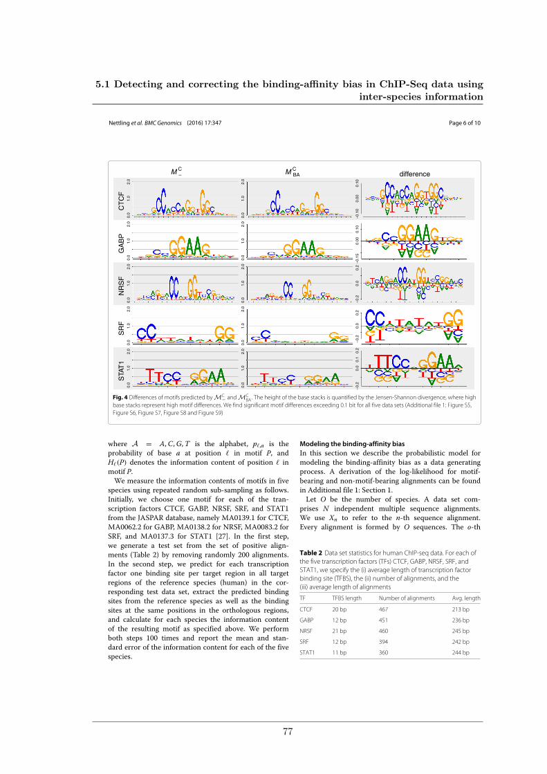
Nettling et al. BMC Genomics (2016) 17:347 Page 6 of 100.

01.

02.

0

0.0

1.0

2.0

−0.

100.

000.

10

0.0

1.0

2.0

0.0

1.0

2.0

−0.

150.

000.

10

0.0

1.0

2.0

0.0

1.0

2.0

−0.

20.

00.

2

0.0

1.0

2.0

0.0

1.0

2.0

−0.

20.

00.

2

0.0

1.0

2.0

0.0

1.0

2.0

−0.

20.

00.

10.

2

STA

T1

SR

FN

RS

FG

AB

PC

TC

F

M –C M BA

Cdifference

Fig. 4 Differences of motifs predicted byMC− andMCBA. The height of the base stacks is quantified by the Jensen-Shannon divergence, where high

base stacks represent high motif differences. We find significant motif differences exceeding 0.1 bit for all five data sets (Additional file 1: Figure S5,Figure S6, Figure S7, Figure S8 and Figure S9)

where A = A,C,G,T is the alphabet, p�,a is theprobability of base a at position � in motif P, andH�(P) denotes the information content of position � inmotif P.We measure the information contents of motifs in five

species using repeated random sub-sampling as follows.Initially, we choose one motif for each of the tran-scription factors CTCF, GABP, NRSF, SRF, and STAT1from the JASPAR database, namely MA0139.1 for CTCF,MA0062.2 for GABP, MA0138.2 for NRSF, MA0083.2 forSRF, and MA0137.3 for STAT1 [27]. In the first step,we generate a test set from the set of positive align-ments (Table 2) by removing randomly 200 alignments.In the second step, we predict for each transcriptionfactor one binding site per target region in all targetregions of the reference species (human) in the cor-responding test data set, extract the predicted bindingsites from the reference species as well as the bindingsites at the same positions in the orthologous regions,and calculate for each species the information contentof the resulting motif as specified above. We performboth steps 100 times and report the mean and stan-dard error of the information content for each of the fivespecies.

Modeling the binding-affinity biasIn this section we describe the probabilistic model formodeling the binding-affinity bias as a data generatingprocess. A derivation of the log-likelihood for motif-bearing and non-motif-bearing alignments can be foundin Additional file 1: Section 1.Let O be the number of species. A data set com-

prises N independent multiple sequence alignments.We use Xn to refer to the n-th sequence alignment.Every alignment is formed by O sequences. The o-th

Table 2 Data set statistics for human ChIP-seq data. For each ofthe five transcription factors (TFs) CTCF, GABP, NRSF, SRF, andSTAT1, we specify the (i) average length of transcription factorbinding site (TFBS), the (ii) number of alignments, and the(iii) average length of alignments

TF TFBS length Number of alignments Avg. length

CTCF 20 bp 467 213 bp

GABP 12 bp 451 236 bp

NRSF 21 bp 460 245 bp

SRF 12 bp 394 242 bp

STAT1 11 bp 360 244 bp

5.1 Detecting and correcting the binding-affinity bias in ChIP-Seq data usinginter-species information

77

Page 88

Nettling et al. BMC Genomics (2016) 17:347 Page 7 of 10

sequence is denoted by X .,on . By convention, the refer-

ence species (that in which the selection process hastaken place) is species 1. Each sequence of alignmentXn is composed of Ln nucleotides. We denote by Xu,o

nthe u-th nucleotide of the o-th sequence of the n-th alignment. All nucleotides are presented by the setA = {A,C,G,T}.We assume the existence of a common ancestor of all

of O species. The sequence of the common ancestor ofthe n-th alignment is a hidden variable Yn, with Yu

n rep-resenting its u-th nucleotide. The substitution probabilitythat nucleotide Yu

n is substituted by the nucleotide Xu,on is

denoted by the variable γo.An alignment Xn may contain a binding site or not. This

is denoted by the variable Mn. The length of the bindingsite is denoted by the variable W and the position of thebinding site in alignment Xn is denoted by the variable �n.The n-th alignment Xn is sampled as follows. The first

decision to be made is whether or not the alignment con-tains a binding site. This is denoted by variableMn whichfollows a Bernoulli distribution with parameter 1 − α.Thus, whenever variable Mn is equal to 1 (M1

n), the align-ment contains a binding site and when Mn is equal to 0(M0

n), it does not.Thus, parameter α is the probability that alignment Xn

contains no binding site. If α equals 0, the sampled data isuncontaminated, because all alignments contain a copy ofthe binding site. The larger the value of α, the higher thepercentage of non motif-bearing alignments in the sam-pled data. A value of α equal to 1 models a data set whereno binding sites are present.Next we introduce the data generating process for non-

motif-bearing alignments and later we explain that formotif-bearing alignments.

1. Sample the primordial sequence as follows: For eachposition u of the sequence sample nucleotide Yu

nfrom the background equilibrium distribution π0independent of the previous nucleotides.

2. For each of the descent species o ∈ {1, . . . ,O},sample its sequence given the primordial sequence asfollows: To sample nucleotide u of the descentspecies o, we apply to nucleotide u of the primordialsequence the F81 [28] mutation model with thebackground equilibrium distribution π0 and thesubstitution probability γo.

The generating process for motif-bearing sequences isslightly more complex, since it has to deal both withthe generation of the binding site and with the selectionprocess. First, we describe how to sample an alignmentwithout taking into account the selection process. Sec-ond, we show how to modify this procedure so that theselection process is considered.

Sample a motif-bearing alignment Xn as follows:

1. Sample the start position of the binding site �n fromthe uniform distribution.

2. Sample the primordial sequence. For each position uof the sequence outside the binding site, we samplenucleotide Yu

n from the background equilibriumdistribution π0. For each position u of the bindingsite, we sample nucleotide Yu

n from the equilibriumdistribution πu−�n+1.

3. For each of the descent species o ∈ {1, . . . ,O},sample its sequence X .,o

n as follows: For each positionu of the descent species o outside the binding site,apply to nucleotide Xu,o

n of the primordial sequencethe F81 mutation model taking as equilibriumdistribution π0. For each position u of the descentspecies o inside the binding site, apply to nucleotideXu,on of the primordial sequence the F81 mutation

model taking as equilibrium distribution πu−�n+1.

Finally, to model the selection process, we introducethe variable β . β is used to quantify the degree of thebinding-affinity bias in the reference species. We assumethat a transcription factor binds binding site B with aprobability proportional to p(B|π)β−1. As B occurs in vivowith probability p(B|π), it occurs in the set of immuno-precipitated sequences with a probability proportional top(B|π) · p(B|π)β−1 = p(B|π)β .We can interpret the meaning of β as follows: If β is

greater than one, low-affinity binding sites are more fre-quently rejected with respect to p(B) and high-affinitybinding sites are less frequently rejected with respect top(B). This leads to an under-representation of low-affinitybinding sites and an over-representation of high-affinitybinding sites in the ChIP-seq data set, thus modeling adata set that is affected by the binding-affinity bias. Ifβ is equal to one, low-affinity binding sites are rejectedas frequently as high-affinity binding sites, leading toa representative set of binding sites in the ChIP-seqdata set, which is not affected by the binding-affinitybias.Based on that selection model, sample a motif-bearing

alignment that has passed the selection process as follows:

1. Sample a motif-bearing alignment disregarding theselection process following the procedure specifiedabove.

2. Decide whether the alignment is accepted or rejectedbased on the probability of acceptance of the bindingsite found at the reference species. If the alignment isrejected, go to step 1.

Thus, we denote (i) the model with α = 0 and β = 1by M−−, (ii) the model with with α > 0 and β = 1 by

5. PREDICTING TRANSCRIPTION FACTOR BINDING SITES USINGPHYLOGENETIC FOOTPRINTING

78

Page 89

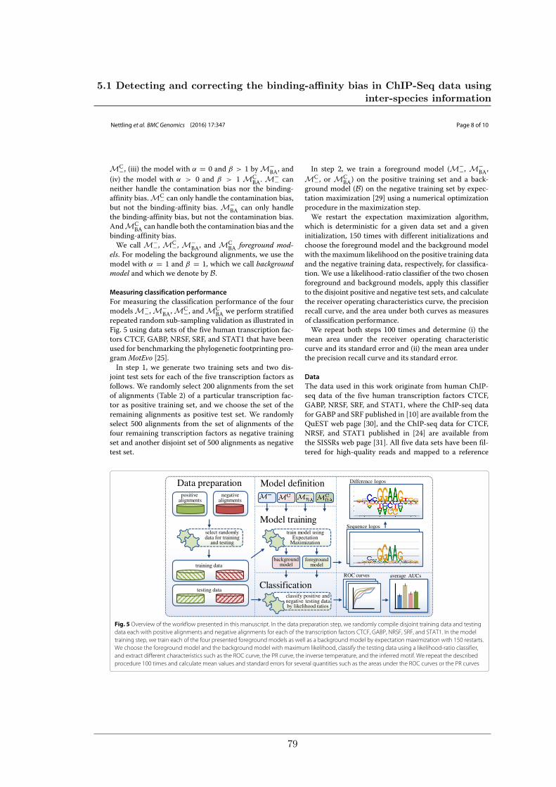
Nettling et al. BMC Genomics (2016) 17:347 Page 8 of 10

MC−, (iii) the model with α = 0 and β > 1 by M−BA, and

(iv) the model with α > 0 and β > 1 MCBA. M

−− canneither handle the contamination bias nor the binding-affinity bias.MC− can only handle the contamination bias,but not the binding-affinity bias. M−

BA can only handlethe binding-affinity bias, but not the contamination bias.AndMC

BA can handle both the contamination bias and thebinding-affinity bias.We call M−−, MC−, M−

BA, and MCBA foreground mod-

els. For modeling the background alignments, we use themodel with α = 1 and β = 1, which we call backgroundmodel and which we denote by B.

Measuring classification performanceFor measuring the classification performance of the fourmodels M−−, M−

BA, MC−, and MCBA we perform stratified

repeated random sub-sampling validation as illustrated inFig. 5 using data sets of the five human transcription fac-tors CTCF, GABP, NRSF, SRF, and STAT1 that have beenused for benchmarking the phylogenetic footprinting pro-gramMotEvo [25].In step 1, we generate two training sets and two dis-

joint test sets for each of the five transcription factors asfollows. We randomly select 200 alignments from the setof alignments (Table 2) of a particular transcription fac-tor as positive training set, and we choose the set of theremaining alignments as positive test set. We randomlyselect 500 alignments from the set of alignments of thefour remaining transcription factors as negative trainingset and another disjoint set of 500 alignments as negativetest set.

In step 2, we train a foreground model (M−−, M−BA,

MC−, or MCBA) on the positive training set and a back-

ground model (B) on the negative training set by expec-tation maximization [29] using a numerical optimizationprocedure in the maximization step.We restart the expectation maximization algorithm,

which is deterministic for a given data set and a giveninitialization, 150 times with different initializations andchoose the foreground model and the background modelwith themaximum likelihood on the positive training dataand the negative training data, respectively, for classifica-tion. We use a likelihood-ratio classifier of the two chosenforeground and background models, apply this classifierto the disjoint positive and negative test sets, and calculatethe receiver operating characteristics curve, the precisionrecall curve, and the area under both curves as measuresof classification performance.We repeat both steps 100 times and determine (i) the

mean area under the receiver operating characteristiccurve and its standard error and (ii) the mean area underthe precision recall curve and its standard error.

DataThe data used in this work originate from human ChIP-seq data of the five human transcription factors CTCF,GABP, NRSF, SRF, and STAT1, where the ChIP-seq datafor GABP and SRF published in [10] are available from theQuEST web page [30], and the ChIP-seq data for CTCF,NRSF, and STAT1 published in [24] are available fromthe SISSRs web page [31]. All five data sets have been fil-tered for high-quality reads and mapped to a reference

testing data

Data preparation

Model training

Model definitionpositive

alignments

training data

Classification

negativealignments

foregroundmodel

select randomlydata for training

and testing

backgroundmodel

train model usingExpectation

Maximization

classify positive andnegative testing databy likelihood ratios

Sequence logos

Difference logos

ROC curves average AUCs

Fig. 5 Overview of the workflow presented in this manuscript. In the data preparation step, we randomly compile disjoint training data and testingdata each with positive alignments and negative alignments for each of the transcription factors CTCF, GABP, NRSF, SRF, and STAT1. In the modeltraining step, we train each of the four presented foreground models as well as a background model by expectation maximization with 150 restarts.We choose the foreground model and the background model with maximum likelihood, classify the testing data using a likelihood-ratio classifier,and extract different characteristics such as the ROC curve, the PR curve, the inverse temperature, and the inferred motif. We repeat the describedprocedure 100 times and calculate mean values and standard errors for several quantities such as the areas under the ROC curves or the PR curves

5.1 Detecting and correcting the binding-affinity bias in ChIP-Seq data usinginter-species information

79

Page 90

Nettling et al. BMC Genomics (2016) 17:347 Page 9 of 10

genome [10, 24], and peak calling has been performed byMACS [32]. Peaks have been extended or cropped to 400bp, binding regions that potentially comprise more thanone of the five transcription factors have been removed,and the 900 binding regions with the highest MACSscore have been retained [25]. Orthologous regions frommouse, dog, cow, monkey, horse, and opossum have beenextracted from the UCSC database [33], multiple align-ments of these orthologous regions have been obtainedusing T-Coffee [34], and these multiple alignments arekindly provided by [25].To prepare ungapped alignments from these gapped

data sets of the five transcription factors CTCF, GABP,NRSF, SRF, and STAT1, we perform the following threesteps. (i) Remove the species that cause the highest num-ber of gaps in all alignments. Accordingly, we removemouse and opossum and keep orthologous regions fromhuman, monkey, cow, dog, and horse. (ii) Remove allcolumns in each of the alignments that contain at leastone gap to obtain ungapped alignments. (iii) Remove allungapped alignments that are shorter than 21 bp, whichis the length of the longest motif (NRSF) in the performedstudies. Table 2 shows details about the resulting data. Alldata are available as Additional file 2.

Visualizing motif differences with DiffLogoWe used the R package DiffLogo [35] to depict the differ-ences between the predicted motifs of the models M−−,M−

BA, MC−, and MCBA. DiffLogo is an open source soft-

ware that is capable of depicting the differences betweenmultiple motifs [35]. This is realized by visualizing all pair-wise differences in anN×N–grid with an empty diagonal.Each entry in the grid is called difference logo. The degreeof difference of two motifs is calculated by the sum of allstack heights in the corresponding difference logo and isindicated by the background color from red (most dissimi-lar among all motif pairs) to green (most similar among allmotif pairs). The individual sequence logos of the motifsare shown above the table.A single difference logo depicts the position-specific dif-

ferences between the base distributions of two sequencemotifs. Differences are visualized using a stack of basesfor each motif position. The height of each base stackis calculated by the Jensen-Shannon divergence, whichis proportional to the degree of base distribution dis-similarity. The Jensen-Shannon divergence is zero if bothbase distributions are identical, increases with increas-ing difference of the two base distributions, and reaches amaximum of 2 bit if the two base distributions are maxi-mally different, i.e., if two bases occur only in one of thetwo motifs each with a probability of 1/2 and the othertwo bases occur only in the other motif each with a prob-ability of 1/2. The height of each base within a stack isgiven by the difference of abundance. Thus, the height of

a base is proportional to the degree of differential symbolabundance. Bases with a positive height indicate a gain ofabundance and bases with a negative height indicate a lossof abundance. The stack height in the positive directionmust be equal to the stack height in the negative direction,because the sum of base abundance gain must be equal tothe sum of base abundance loss.

Additional files

Additional file 1: Supplementary Methods, Results, Figures, andExamples. This file is structured in four sections.In section 1,Modeling the binding-affinity bias, we describe how todetermine the likelihood of non-motif-bearing and motif-bearingalignments modeling the contamination bias and the binding-affinity bias.In section 2, Example interpretation of difference logos, we give an exemplaryinterpretation of some difference logos.Section 3, Supplementary Figures, contains supplementary Figures S1-S18.Section 4, Supplementary Tables, contains supplementary Tables S1-S10.(PDF 3492 kb)

Additional file 2: Sequence data. This archive contains data files ofgap-free alignments of the ChIP-seq positive regions for each of thetranscription factors CTCF, GABP, NRSF, SRF, and STAT1 in FASTA format.(ZIP 645 kb)

Competing interestsThe authors declare that they have no competing interests.

Authors’ contributionsMN and IG developed the key idea. MN and JC developed the computationalmethods. MN and HT performed the studies. All authors wrote, read, andapproved the final manuscript.

AcknowledgementsWe thank Lothar Altschmied, Helmut Bäumlein, Sven-Erik Behrens, KarinBreunig, Jan Grau, Katrin Hoffmann, Robert Paxton, Patrice Peterson, andMarcel Quint for valuable discussions and DFG (grant no. GR3526/1), Gencat(2014 SGR 118), and Collectiveware (TIN2015-66863-C2-1-R) for financialsupport.

Author details1Institute of Computer Science, Martin Luther University, Halle (Saale),Germany. 2Leibniz Institute of Plant Biochemistry, Halle (Saale), Germany.3IIIA-CSIC, Campus UAB, Barcelona, Spain. 4German Centre for IntegrativeBiodiversity Research (iDiv) Halle-Jena-Leipzig, Leipzig, Germany.

Received: 15 December 2015 Accepted: 28 April 2016

References1. Nowrousian M. Next-generation sequencing techniques for eukaryotic

microorganisms: sequencing-based solutions to biological problems.Eukaryot Cell. 2010;9(9):1300–10.

2. Villar D, Flicek P, Odom DT. Evolution of transcription factor binding inmetazoans - mechanisms and functional implications. Nat Rev Genet.2014;15(4):221–33.

3. Park PJ. Chip–seq: advantages and challenges of a maturing technology.Nat Rev Genet. 2009;10(10):669–80.

4. Furey TS. Chip–seq and beyond: new and improved methodologies todetect and characterize protein–dna interactions. Nat Rev Genet.2012;13(12):840–52.

5. Landt SG, Marinov GK, Kundaje A, Kheradpour P, Pauli F, Batzoglou S,Bernstein BE, Bickel P, Brown JB, Cayting P, et al. Chip-seq guidelines andpractices of the encode and modencode consortia. Genome Res.2012;22(9):1813–31.

5. PREDICTING TRANSCRIPTION FACTOR BINDING SITES USINGPHYLOGENETIC FOOTPRINTING

80

Page 91

Nettling et al. BMC Genomics (2016) 17:347 Page 10 of 10

6. Alipanahi B, Delong A, Weirauch MT, Frey BJ. Predicting the sequencespecificities of DNA- and RNA-binding proteins by deep learning. NatBiotechnol. 2015;33(8):831–8. doi:10.1038/nbt.3300.

7. Hawkins J, Grant C, Noble WS, Bailey TL. Assessing phylogenetic motifmodels for predicting transcription factor binding sites. Bioinformatics.2009;25(12):339–47.

8. Gomes AL, Abeel T, Peterson M, Azizi E, Lyubetskaya A, Carvalho L,Galagan J. Decoding chip-seq with a double-binding signal refinesbinding peaks to single-nucleotides and predicts cooperative interaction.Genome Res. 2014;24(10):1686–97.

9. Jain D, Baldi S, Zabel A, Straub T, Becker PB. Active promoters give riseto false positive ‘Phantom Peaks’ in ChIP-seq experiments. Nucleic AcidsRes. 2015;43(14):6959–68. doi:10.1093/nar/gkv637.

10. Valouev A, Johnson A, David S and. Sundquist, Medina C, Anton E,Batzoglou S, Myers RM, Sidow A. Genome-wide analysis of transcriptionfactor binding sites based on ChIP-Seq data. Nat Methods. 2008;5(9):829–34.

11. Rye MB, Sætrom P, Drabløs F. A manually curated chip-seq benchmarkdemonstrates room for improvement in current peak-finder programs.Nucleic Acids Res. 2011;39(4):e25. doi:10.1093/nar/gkq1187.

12. Jung YL, Luquette LJ, Ho JWK, Ferrari F, Tolstorukov M, Minoda A,Issner R, Epstein CB, Karpen GH, Kuroda MI, Park PJ. Impact ofsequencing depth in ChIP-seq experiments. Nucleic Acids Res. 2014;42(9):178–4. doi:10.1093/nar/gku178.

13. Zhang Y, Liu T, Meyer CA, Eeckhoute J, Johnson DS, Bernstein BE,Nusbaum C, Myers RM, Brown M, Li W, et al. Model-based analysis ofchip-seq (macs). Genome Biol. 2008;9(9):137.

14. Nix DA, Courdy SJ, Boucher KM. Empirical methods for controlling falsepositives and estimating confidence in chip-seq peaks. BMCBioinformatics. 2008;9(1):523.

15. Bailey TL, Krajewski P, Ladunga I, Lefebvre C, Li Q, Liu T, Madrigal P,Taslim C, Zhang J. Practical guidelines for the comprehensive analysis ofChIP-seq data. PLoS Comput Biol. 2013;9(11):e1003326.

16. Håndstad T, Rye MB, Drabløs F, Sætrom P. A ChIP-Seq Benchmark ShowsThat Sequence Conservation Mainly Improves Detection of StrongTranscription Factor Binding Sites. PLoS ONE. 2011;6(4):18430.doi:10.1371/journal.pone.0018430.

17. Ross MG, Russ C, Costello M, Hollinger A, Lennon NJ, Hegarty R,Nusbaum C, Jaffe DB. Characterizing and measuring bias in sequencedata. Genome Biol. 2013;14(5):51.

18. Park D, Lee Y, Bhupindersingh G, Iyer VR. Widespread MisinterpretableChIP-seq Bias in Yeast. PloS One. 2013;8(12):83506.

19. Teytelman L, Thurtle DM, Rine J, van Oudenaarden A. Highly expressedloci are vulnerable to misleading ChIP localization of multiple unrelatedproteins. Proc Nat Acad Sci. 2013;110(46):18602–7.

20. Elliott JH, Grimshaw J, Altman R, Bero L, Goodman SN, Henry D,Macleod M, Tovey D, Tugwell P, White H, Sim I. Informatics: Make senseof health data. Nature. 2015;527:31–2.

21. Bailey TL, Elkan C. The value of prior knowledge in discovering motifswith MEME. Ismb. 1995;3:21–9.

22. Wilbanks EG, Facciotti MT. Evaluation of algorithm performance inchip-seq peak detection. PloS one. 2010;5(7):11471.

23. Schneider TD, Stormo GD, Gold L, Ehrenfeucht A. Information contentof binding sites on nucleotide sequences. J Mol Biol. 1986;188(3):415–31.

24. Jothi R, Cuddapah S, Barski A, Cui K, Zhao K. Genome-wideidentification of in vivo protein-DNA binding sites from ChIP-Seq data.Nucl Acids Res. 2008;36(16):5221–31. doi:10.1093/nar/gkn488. http://nar.oxfordjournals.org/cgi/reprint/36/16/5221.pdf.

25. Arnold P, Erb I, Pachkov M, Molina N, van Nimwegen E. MotEvo:integrated Bayesian probabilistic methods for inferring regulatory sitesand motifs on multiple alignments of DNA sequences. Bioinformatics.2012;28(4):487–94. doi:10.1093/bioinformatics/btr695.

26. Sober E. The principle of parsimony. Brit J Philos Sci. 1981;32(2):145–56.27. Mathelier A, Zhao X, Zhang AW, Parcy F, Worsley-Hunt R, Arenillas DJ,

Buchman S, Chen C-YY, Chou A, Ienasescu H, Lim J, Shyr C, Tan G,Zhou M, Lenhard B, Sandelin A, Wasserman WW. JASPAR 2014: anextensively expanded and updated open-access database oftranscription factor binding profiles. Nucleic Acids Res. 2014;42(Databaseissue):142–7. doi:10.1093/nar/gkt997.

28. Felsenstein J. Evolutionary trees from DNA sequences: a maximumlikelihood approach. J Mol Evol. 1981;17(6):368–76.

29. Lawrence CE, Reilly AA. An expectation maximization (em) algorithm forthe identification and characterization of common sites in unalignedbiopolymer sequences. Proteins: Struct Funct Bioinformatics. 1990;7(1):41–51.

30. Quantitative Enrichment of Sequence Tags: QuEST. http://mendel.stanford.edu/sidowlab/downloads/quest/. Accessed 29 Mar 2016.

31. ChIP-Seq Data Analysis: Identification of Protein–DNA Binding Sites withSISSRs Peak-Finder. http://dir.nhlbi.nih.gov/papers/lmi/epigenomes/sissrs/. Accessed 29 Mar 2016.

32. Zhang Y, Liu T, Meyer CA, Eeckhoute J, Johnson DS, Bernstein BE,Nusbaum C, Myers RM, Brown M, Li W, Liu XS. Model-based analysis ofChIP-seq (MACS). Genome Biol. 2008;9(9):137.doi:10.1186/gb-2008-9-9-r137.

33. Karolchik D, Kuhn RM, Baertsch R, Barber GP, Clawson H, Diekhans M,Giardine B, Harte RA, Hinrichs AS, Hsu F, Kober KM, Miller W, PedersenJS, Pohl A, Raney BJ, Rhead B, Rosenbloom KR, Smith KE, Stanke M,Thakkapallayil A, Trumbower H, Wang T, Zweig AS, Haussler D, Kent WJ.The UCSC genome browser database: 2008 update. Nucleic Acids Res.2008;36(suppl 1):773–9. doi:10.1093/nar/gkm966.

34. Notredame C, Higgins DG, Heringa J. T-Coffee: A novel method for fastand accurate multiple sequence alignment. J Mol Biol. 2000;302(1):205–17. doi:10.1006/jmbi.2000.4042.

35. Nettling M, Treutler H, Grau J, Keilwagen J, Posch S, Grosse I. DiffLogo: acomparative visualization of sequence motifs. BMC Bioinf. 2015;16(1):1.

• We accept pre-submission inquiries

• Our selector tool helps you to find the most relevant journal

• We provide round the clock customer support

• Convenient online submission

• Thorough peer review

• Inclusion in PubMed and all major indexing services

• Maximum visibility for your research

Submit your manuscript atwww.biomedcentral.com/submit

Submit your next manuscript to BioMed Central and we will help you at every step:

5.1 Detecting and correcting the binding-affinity bias in ChIP-Seq data usinginter-species information

81

Page 92

5. PREDICTING TRANSCRIPTION FACTOR BINDING SITES USINGPHYLOGENETIC FOOTPRINTING

5.2 Unrealistic phylogenetic trees may improve phylogeneticfootprinting

M Nettling, H Treutler, J Cerquides, I Grosse. 2017. Unrealistic phylogenetic trees mayimprove phylogenetic footprinting. Bioinformaticsdoi:10.1093/bioinformatics/btx033

82

Page 93

Nettling et al. BMC Bioinformatics (2017) 18:141 DOI 10.1186/s12859-017-1495-1

RESEARCH ARTICLE Open Access

Combining phylogenetic footprintingwith motif models incorporating intra-motifdependenciesMartin Nettling1*, Hendrik Treutler2, Jesus Cerquides3 and Ivo Grosse1,4

Abstract

Background: Transcriptional gene regulation is a fundamental process in nature, and the experimental andcomputational investigation of DNA binding motifs and their binding sites is a prerequisite for elucidating thisprocess. Approaches for de-novo motif discovery can be subdivided in phylogenetic footprinting that takes intoaccount phylogenetic dependencies in aligned sequences of more than one species and non-phylogeneticapproaches based on sequences from only one species that typically take into account intra-motif dependencies. Ithas been shown that modeling (i) phylogenetic dependencies as well as (ii) intra-motif dependencies separatelyimproves de-novo motif discovery, but there is no approach capable of modeling both (i) and (ii) simultaneously.

Results: Here, we present an approach for de-novo motif discovery that combines phylogenetic footprinting withmotif models capable of taking into account intra-motif dependencies. We study the degree of intra-motifdependencies inferred by this approach from ChIP-seq data of 35 transcription factors. We find that significantintra-motif dependencies of orders 1 and 2 are present in all 35 datasets and that intra-motif dependencies of order 2are typically stronger than those of order 1. We also find that the presented approach improves the classificationperformance of phylogenetic footprinting in all 35 datasets and that incorporating intra-motif dependencies of order2 yields a higher classification performance than incorporating such dependencies of only order 1.

Conclusion: Combining phylogenetic footprinting with motif models incorporating intra-motif dependencies leadsto an improved performance in the classification of transcription factor binding sites. This may advance ourunderstanding of transcriptional gene regulation and its evolution.

Keywords: ChIP-Seq, Phylogenetic footprinting, Evolution, Transcription factor binding sites, Gene regulation

BackgroundGene regulation is an essential process in every livingorganism that controls the activity of gene expressionand enables the concerted up- and down-regulation ofgene products. Gene regulation involves a wide range ofsub-processes such as transcriptional regulation includ-ing DNA methylation [1], histon modifications [2], andpromotor escaping [3] as well as post-transcriptional reg-ulation including modulated mRNA decay [4], siRNAinterference [5, 6], and alternative splicing [7, 8]. Oneimportant process in gene regulation is the interaction

*Correspondence: [email protected] of Computer Science, Martin Luther University Halle-Wittenberg,Halle, GermanyFull list of author information is available at the end of the article

of transcription factors (TFs) with their correspondingtranscription factor binding sites (TFBSs) [9, 10]. Thealgorithmic discovery of TFBSs and the simultaneousinference of their motifs is known as de-novo motif dis-covery and a challenging task in bioinformatics. Manydifferent approaches exist for de-novo motif discovery,which can be divided in two groups.The first group comprises approaches based on

sequences of only one species, which we refer to as one-species approaches in this work, using statistical mod-els for the binding of TFs to their TFBSs. One of themost popular motif models is the simple position weightmatrix (PWM) model, which does not take into accountany dependency between different positions of the sameTFBS, but there are also more complex motif models that

© The Author(s). 2017 Open Access This article is distributed under the terms of the Creative Commons Attribution 4.0International License (http://creativecommons.org/licenses/by/4.0/), which permits unrestricted use, distribution, andreproduction in any medium, provided you give appropriate credit to the original author(s) and the source, provide a link to theCreative Commons license, and indicate if changes were made. The Creative Commons Public Domain Dedication waiver(http://creativecommons.org/publicdomain/zero/1.0/) applies to the data made available in this article, unless otherwise stated.

5.2 Unrealistic phylogenetic trees may improve phylogenetic footprinting

83

Page 94

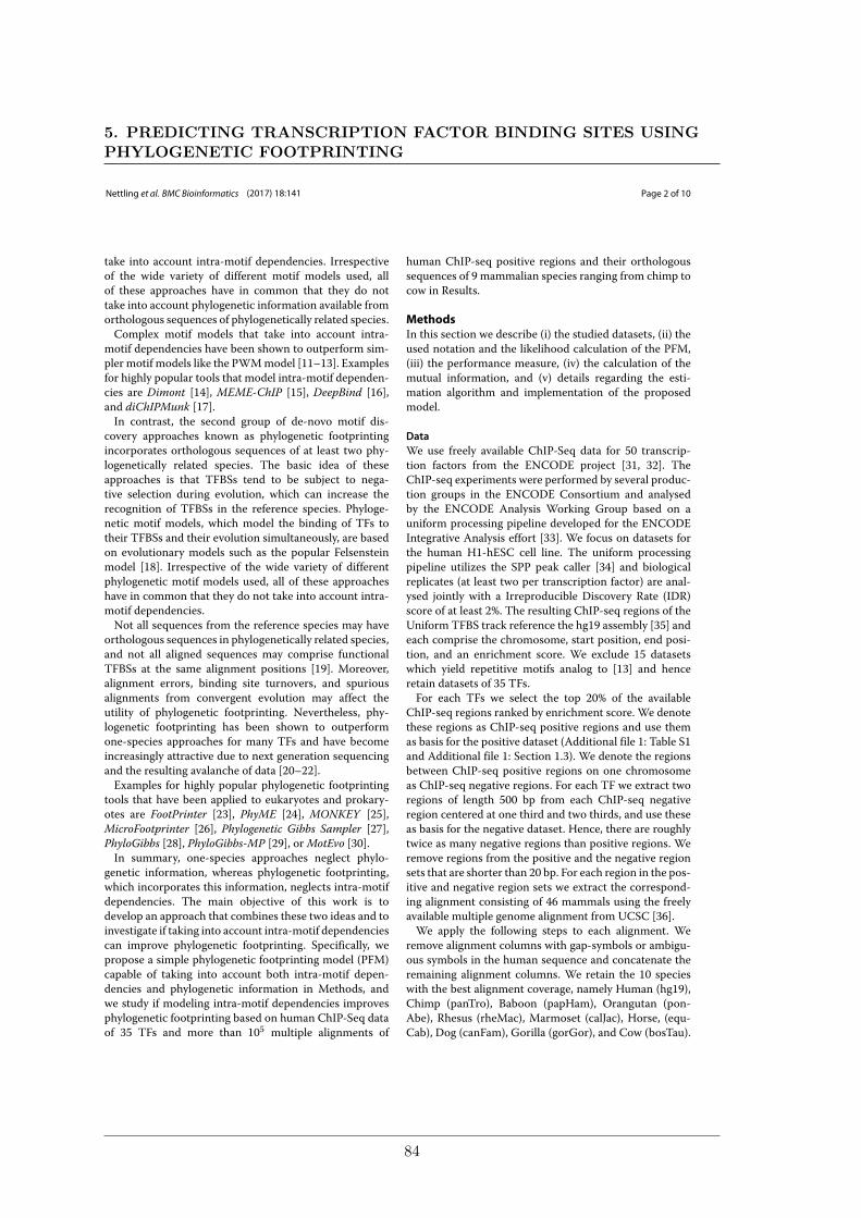
Nettling et al. BMC Bioinformatics (2017) 18:141 Page 2 of 10

take into account intra-motif dependencies. Irrespectiveof the wide variety of different motif models used, allof these approaches have in common that they do nottake into account phylogenetic information available fromorthologous sequences of phylogenetically related species.Complex motif models that take into account intra-

motif dependencies have been shown to outperform sim-pler motif models like the PWMmodel [11–13]. Examplesfor highly popular tools that model intra-motif dependen-cies are Dimont [14], MEME-ChIP [15], DeepBind [16],and diChIPMunk [17].In contrast, the second group of de-novo motif dis-

covery approaches known as phylogenetic footprintingincorporates orthologous sequences of at least two phy-logenetically related species. The basic idea of theseapproaches is that TFBSs tend to be subject to nega-tive selection during evolution, which can increase therecognition of TFBSs in the reference species. Phyloge-netic motif models, which model the binding of TFs totheir TFBSs and their evolution simultaneously, are basedon evolutionary models such as the popular Felsensteinmodel [18]. Irrespective of the wide variety of differentphylogenetic motif models used, all of these approacheshave in common that they do not take into account intra-motif dependencies.Not all sequences from the reference species may have

orthologous sequences in phylogenetically related species,and not all aligned sequences may comprise functionalTFBSs at the same alignment positions [19]. Moreover,alignment errors, binding site turnovers, and spuriousalignments from convergent evolution may affect theutility of phylogenetic footprinting. Nevertheless, phy-logenetic footprinting has been shown to outperformone-species approaches for many TFs and have becomeincreasingly attractive due to next generation sequencingand the resulting avalanche of data [20–22].Examples for highly popular phylogenetic footprinting

tools that have been applied to eukaryotes and prokary-otes are FootPrinter [23], PhyME [24], MONKEY [25],MicroFootprinter [26], Phylogenetic Gibbs Sampler [27],PhyloGibbs [28], PhyloGibbs-MP [29], orMotEvo [30].In summary, one-species approaches neglect phylo-

genetic information, whereas phylogenetic footprinting,which incorporates this information, neglects intra-motifdependencies. The main objective of this work is todevelop an approach that combines these two ideas and toinvestigate if taking into account intra-motif dependenciescan improve phylogenetic footprinting. Specifically, wepropose a simple phylogenetic footprinting model (PFM)capable of taking into account both intra-motif depen-dencies and phylogenetic information in Methods, andwe study if modeling intra-motif dependencies improvesphylogenetic footprinting based on human ChIP-Seq dataof 35 TFs and more than 105 multiple alignments of

human ChIP-seq positive regions and their orthologoussequences of 9 mammalian species ranging from chimp tocow in Results.

MethodsIn this section we describe (i) the studied datasets, (ii) theused notation and the likelihood calculation of the PFM,(iii) the performance measure, (iv) the calculation of themutual information, and (v) details regarding the esti-mation algorithm and implementation of the proposedmodel.

DataWe use freely available ChIP-Seq data for 50 transcrip-tion factors from the ENCODE project [31, 32]. TheChIP-seq experiments were performed by several produc-tion groups in the ENCODE Consortium and analysedby the ENCODE Analysis Working Group based on auniform processing pipeline developed for the ENCODEIntegrative Analysis effort [33]. We focus on datasets forthe human H1-hESC cell line. The uniform processingpipeline utilizes the SPP peak caller [34] and biologicalreplicates (at least two per transcription factor) are anal-ysed jointly with a Irreproducible Discovery Rate (IDR)score of at least 2%. The resulting ChIP-seq regions of theUniform TFBS track reference the hg19 assembly [35] andeach comprise the chromosome, start position, end posi-tion, and an enrichment score. We exclude 15 datasetswhich yield repetitive motifs analog to [13] and henceretain datasets of 35 TFs.For each TFs we select the top 20% of the available

ChIP-seq regions ranked by enrichment score. We denotethese regions as ChIP-seq positive regions and use themas basis for the positive dataset (Additional file 1: Table S1and Additional file 1: Section 1.3). We denote the regionsbetween ChIP-seq positive regions on one chromosomeas ChIP-seq negative regions. For each TF we extract tworegions of length 500 bp from each ChIP-seq negativeregion centered at one third and two thirds, and use theseas basis for the negative dataset. Hence, there are roughlytwice as many negative regions than positive regions. Weremove regions from the positive and the negative regionsets that are shorter than 20 bp. For each region in the pos-itive and negative region sets we extract the correspond-ing alignment consisting of 46 mammals using the freelyavailable multiple genome alignment from UCSC [36].We apply the following steps to each alignment. We

remove alignment columns with gap-symbols or ambigu-ous symbols in the human sequence and concatenate theremaining alignment columns. We retain the 10 specieswith the best alignment coverage, namely Human (hg19),Chimp (panTro), Baboon (papHam), Orangutan (pon-Abe), Rhesus (rheMac), Marmoset (calJac), Horse, (equ-Cab), Dog (canFam), Gorilla (gorGor), and Cow (bosTau).

5. PREDICTING TRANSCRIPTION FACTOR BINDING SITES USINGPHYLOGENETIC FOOTPRINTING

84

Page 95

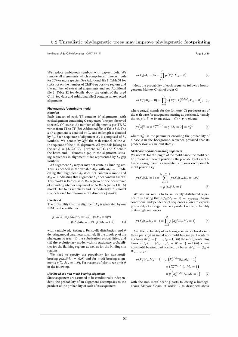
Nettling et al. BMC Bioinformatics (2017) 18:141 Page 3 of 10

We replace ambiguous symbols with gap-symbols. Weremove all alignments which comprise no base symbolsfor 20% or more species. See Additional file 1: Table S1 forstatistics on the number of ChIP-Seq positive regions andthe number of extracted alignments and see Additionalfile 1: Table S2 for details about the origin of the usedChIP-Seq data and Additional file 2 contains all extractedalignments.

Phylogenetic footprinting modelNotationEach dataset of each TF contains N alignments, witheach alignment containingO sequences (one per observedspecies). Of course the number of alignments per TF, N,varies from TF to TF (See Additional file 1: Table S1). Then-th alignment is denoted by Xn and its length is denotedby Ln. Each sequence of alignment Xn is composed of Lnsymbols. We denote by Xu,o

n the u-th symbol of the o-th sequence of the n-th alignment. All symbols belong tothe set A = {A,C,G,T ,−} where A,C,G, and T denotethe bases and − denotes a gap in the alignment. Miss-ing sequences in alignment n are represented by Ln gapsymbols.An alignment Xn may or may not contain a binding site.

This is encoded in the variable Mn, with Mn = 0 indi-cating that alignment Xn does not contain a motif andMn = 1 indicating that alignmentXn does contain a motif.This model is known as ZOOPS (zero or one occurrenceof a binding site per sequence) or NOOPS (noisy OOPS)model. Due to its simplicity and its modularity this modelis widely used for de-novo motif discovery [37–40].

LikelihoodThe probability that the alignment Xn is generated by ourPFM can be written as

p (Xn|θ) = p (Xn|Mn = 0, θ) · p (Mn = 0|θ)

+ p (Xn|Mn = 1, θ) · p (Mn = 1|θ) (1)

with variable Mn taking a Bernoulli distribution and θ

denoting model parameters, namely (i) the topology of thephylogenetic tree, (ii) the substitution probabilities, and(iii) the evolutionary model with its stationary probabili-ties for the flanking regions as well as for the binding siteregions.We need to specify the probability for non-motif-

bearing p(Xn|Mn = 0, θ) and for motif-bearing align-ments p(Xn|Mn = 1, θ). For reasons of clarity we omit θ

in the following.

Likelihood of a non-motif-bearing alignmentSince sequences are assumed to be conditionally indepen-dent, the probability of an alignment decomposes as theproduct of the probability of each of its sequences:

p (Xn|Mn = 0) =O∏

o=1p

(X .,on |Mn = 0

)(2)

Now, the probability of each sequence follows a homo-geneous Markov Chain of order C:

p(X .,on |Mn = 0

) =Ln∏

u=1p

(Xu,on |Xp(u,1),o

n ,Mn = 0), (3)

where p(u, k) stands for the (at most C) predecessors ofthe u-th base for a sequence starting at position k, namelythe set p(u, k) = {v|max(k,u − C) ≤ v < u}, and

p(Xu,on = a|Xp(u,1),o

n = ζ ,Mn = 0)

= πa,ζ0 (4)

where πa,ζ0 is the parameter encoding the probability of

a base a in the background sequence provided that itspredecessors are in joint state ζ .

Likelihood of amotif-bearing alignmentWe noteW for the length of the motif. Since the motif canbe present in different positions, the probability of amotif-bearing assignment is a weighted sum over each possiblemotif position �n:

p (Xn|Mn = 1) =Ln−W+1∑

�n=1p (Xn|�n,Mn = 1, θ , )

× p (�n|Mn = 1) (5)

We assume motifs to be uniformly distributed a pri-ori, thus having that p(�n|Mn = 1) = 1

Ln−W+1 . Again,conditional independence of sequences allows to expressprobability of an alignment as a product of the probabilityof its single sequences

p (Xn|�n,Mn = 1) =O∏

o=1p

(X .,on , �n,Mn = 1

)(6)

And the probability of each single sequence breaks intothree parts: (i) an initial non-motif bearing part contain-ing bases i(�n) = {1, . . . , �n − 1}, (ii) the motif, containingbases m(�n) = {�n, . . . , �n + W − 1} and (iii) a finalnon-motif bearing part formed by bases e(�n) = {�n +W , . . . , Ln} :

p(X .,on |�n,Mn = 1

) = p(Xi(�n),on |�n,Mn = 1

)

×(Xm(�n),on |�n,Mn = 1

)

× p(Xe(�n),on |�n,Mn = 1

)(7)

with the non-motif bearing parts following a homoge-neous Markov Chain of order C as described above

5.2 Unrealistic phylogenetic trees may improve phylogenetic footprinting

85

Page 96

Nettling et al. BMC Bioinformatics (2017) 18:141 Page 4 of 10

and the motif-bearing part following a non-homogeneousMarkov Chain defined as

p(Xm(�n),on |�n,Mn = 1

)

=∏

u∈m(�n)

p(Xu,on |Xp(u,�n),o

n , �n,Mn = 1), (8)

with

p(Xu,on = a|Xp(u,�n),o

n = ζ , �n,Mn = 0)

= πa,ζu−�n+1

(9)

where πa,ζw is a parameter that encodes the probability

of a base a, at position w of the motif provided that itspredecessors are in joint state ζ .

Management of gapsA sequence may have gaps introduced by the alignmentalgorithm. We compute the probability of a gap by sum-ming over all possible nucleotides at that position inthat sequence. For example to assess p

(Xu,on = −|Xp(u,1),o

n

= ζ ,Mn = 0), we use

∑a∈{A,C,G,T} p

(Xu,on = a|Xp(u,1),o

n

= ζ ,Mn = 0).

The used model estimation procedure and the freelyavailable implementation are specified in Methods 5, andrun times are exemplified in Additional file 1: Section 1.6.

Measuring classification performanceWe evaluate all PFMs by a stratified repeated random sub-sampling validation by estimating all PFMs from a trainingset and measuring classification performance on a test setas follows.In step 1, we generate two training sets and two dis-

joint test sets for each of the 35 transcription factorsas follows. We randomly select 70% but maximal 1000alignments from the set of alignments of a particular tran-scription factor as positive training set, and we choose theset of the remaining alignments but maximal 1000 as pos-itive test set. We randomly select 70% but maximal 1000alignments from the corresponding set of negative align-ments of this transcription factor, and we choose the setof the remaining alignments but maximal 1000 as negativetest set.In step 2, we train a foreground model on the posi-

tive training set and a background model on the negativetraining set by expectation maximization [41] using anumerical optimization procedure in the maximizationstep. In all cases, we attempt to find a motif of lengthW = 20 bp. It is known that the motifs of many TFs have alength smaller thanW bp, but adding some possibly unin-formative positions in case of short motifs is less harmfulthan not being able to take into account all motif positions

in case of long motifs. We restart the expectation max-imization algorithm, which is deterministic for a givendataset and a given initialization, 100 times with differ-ent initializations and choose the foreground model andthe background model with the maximum likelihood onthe positive training data and the negative training data,respectively, for classification. We use a likelihood-ratioclassifier of the two chosen foreground and backgroundmodels, apply this classifier to the disjoint positive andnegative test sets, and calculate the area under the receiveroperating characteristics curve and the area underthe precision recall curve as measures of classificationperformance.We repeat both steps 25 times and determine (i) the

mean area under the receiver operating characteristiccurve and its standard error and (ii) the mean area underthe precision recall curve and its standard error.

Relative increase of classification performanceWe compute the relative increase or decrease of the clas-sification performance of the PFM(1) and the PFM(2)relative to the PFM(0), where PFM(C) denotes a PFMstaking into account base dependencies of order C. Wecompute RPFM(C) as the ratio of the improvement of thePFM(C) relative to the PFM(0) divided by the maximumpossible improvement to the PFM(0) as given by

RPFM(C) = AUCPFM(C) − AUCPFM(0)1 − AUCPFM(0)

.

Negative values of RPFM(C) denote a decrease of classifi-cation performance and positive values of RPFM(C) denotean increase of classification performance up to a maxi-mum of RPFM(C) = 1 which denotes perfect classification(provided that the AUC of PFM(0) is smaller than 1).

Mutual informationThe mutual information (MI) is a standard measure forquantifying statistical dependencies. We compute the MIbetween a base at positionw in a motif and itsC precedingbases for w > C as follows

IC(w) = I(Xw,XC

w

)=

∑

a∈AC

∑

b∈Ap

(XCw = a,Xw = b

)

× log2p

(XCw = a,Xw = b

)

p(XCw = a

)p(Xw = b)

where Xw denotes the base at position w and XCw =

(Xw−C , . . . ,Xw−1) denotes the context of Xw. IC(w)

denotes the amount of information in theC-mer ending atposition w− 1 about its adjacent base at position w. IC(w)

is undefined for w ≤ C.We denote the vector of MIs values IC(w) for w ∈ {C +

1, . . . ,W } by IC = (IC(C+1), . . . , IC(W )), whereW is thelength of the motif, and we call this vector MI profile.

5. PREDICTING TRANSCRIPTION FACTOR BINDING SITES USINGPHYLOGENETIC FOOTPRINTING

86

Page 97

Nettling et al. BMC Bioinformatics (2017) 18:141 Page 5 of 10

ImplementationWe implement the proposed PFM based on the freelyavailable Java Framework Jstacs [42]. Among others,Jstacs provides ready-to-use sequence models for reuse,numerical and non-numerical optimization proceduresfor model estimation, serialization of models, and meth-ods for the statistical evaluation of results. In contrast toexisting tools which are typically focused on application,using Jstacs we are able to compare different PFMs in adetailed way by extracting mandatory information aboutthe inferred models and the predicted binding sites.Algorithm 1 shows the pseudocode for inferring a PFM

from a set of alignments. The implementation of theproposed phylogenetic footprinting model is available athttps://github.com/mgledi/PhyFoo/.

Algorithm 1 Motif discovery algorithm for the proposedPFM. Upon random initialization of the model parame-ters we iteratively estimate sequence weights and modelparameters with multiple algorithm restarts, where Rdenotes the number of restarts of the whole algorithm,and S denotes the number of iterations. The result is theset of model parameters with maximum likelihood1: Data: Set of alignments {X1, . . . ,XN }2: for r = 1 . . . R do3: Initialize θ1 randomly4: for s = 1 . . . S do5: E-step:Estimate p(Xm(�n),o

n |�n,Mn = 1, θ s) foreach position �n in each alignment Xn giventhe model parameters θ s (see Eq. 8)

6: M-step: Maximize p(Xn|θ s+1) regardingθ s+1 given all alignments and the probabilitiesp(Xm(�n),o

n |�n,Mn = 1, θ s) (see Eq. 1)7: end for8: Keep θS+1 denoted θr9: end for

10: Result: θ ∈ {θ1, . . . θR} with maximum likelihood

Results and discussionWe propose a model for phylogenetic footprinting that iscapable of taking into account intra-motif dependencies asspecified in Methods 2. Specifically, we model intra-motifdependencies in TFBSs as well as dependencies amongadjacent bases in flanking sequences by Markov modelsof orders 0, 1, and 2, and we denote the proposed PFM byPFM(0), PFM(1), and PFM(2).In the first subsection we study if the proposed PFMs

can capture intra-motif dependencies of orders 1 and 2in ChIP-Seq data of 35 TFs. In the second subsection westudy if modeling base dependencies can improve phy-logenetic footprinting. Both studies are based on humansequences extracted from ENCODE ChIP-seq data [33]

and corresponding orthologous sequences of 9 mam-malian species, yielding 35 data sets comprising 135196multiple sequence alignments with an average length of124 bases (Methods 1).

Intra-motif dependencies can be captured by phylogeneticfootprintingIn this subsection we study to which degree intra-motifdependencies can be captured using the PFMs of orders 1and 2.We measure the degree of intra-motif dependencies of

order 1 between two neighboring bases or of order 2between a dimer and its neighboring base by the MI asdescribed in Methods 4. The MI quantifies the amountof information in a base or a dimer about the neighbor-ing base in units of bits and ranges from 0 bits in caseof statistical independence to 2 bits in case of determin-istic dependency of the considered base on the precedingbase or the preceding dimer.We compute theMI for everyposition of a binding site and call the resulting vector ofMI values MI profile.For each of the 35 TFs, we compute the two MI profiles

of orders 1 and 2 from themotifs obtained by phylogeneticfootprinting using the PFM(2). We present the resulting35 × 2 MI profiles as Additional file 3 and the 2 × 2 MIprofiles of the two TFs CJUN and Nrf as examples inFig. 1a.First, we study the MI profiles of order 1 for these

two TFs. For both TFs we find statistically significantintra-motif dependencies between neighboring bases atall positions. ForCJUN, intra-motif dependencies of order1 are particularly strong at motif positions 2 to 4, yield-ing a maximum MI of 0.52 bits at motif position 4. ForNrf, intra-motif dependencies of order 1 are particularlystrong at motif positions 8 to 11 and 14 to 15, yielding amaximumMI of 0.23 bits at motif position 11.Next, we study the MI profiles of order 2. Again, we find

statistically significant intra-motif dependencies betweendimers and their neighboring bases at all positions forboth CJUN and Nrf. For CJUN, intra-motif dependenciesof order 2 are particularly strong at motif positions 2 to 4,yielding a maximum MI of 0.70 bits at motif position 3.For Nrf, intra-motif dependencies of order 2 are particu-larly strong at motif positions 8 to 11 and 13 to 15, yieldinga maximumMI of 0.28 bit at motif position 11.Moreover, we find that intra-motif dependencies of

order 2 are significantly stronger than the correspondingintra-motif dependencies of order 1 at several positionsfor both CJUN and Nrf. Comparing the MI profiles oforders 1 and 2, we find that the MI profile of order 2 isup to twofold higher than the MI profile of order 1 forCJUN and up to sevenfold higher for Nrf, stating that inboth TFs there are significant intra-motif dependencies of

5.2 Unrealistic phylogenetic trees may improve phylogenetic footprinting

87

Page 98

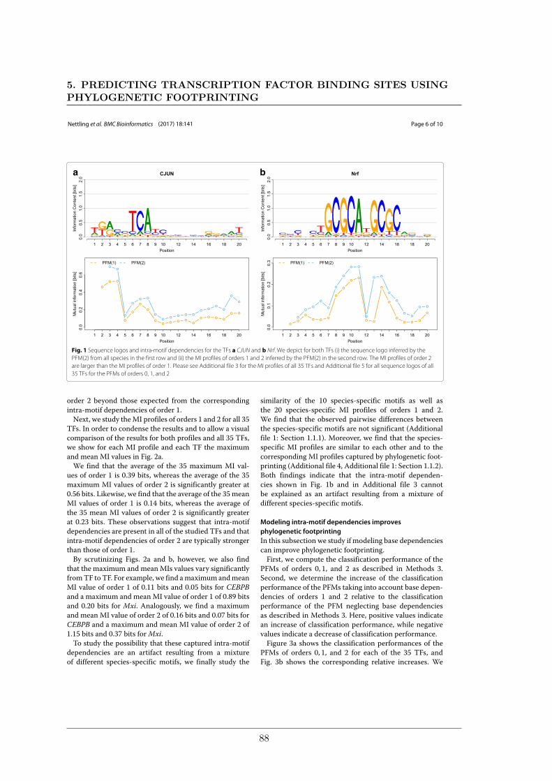
Nettling et al. BMC Bioinformatics (2017) 18:141 Page 6 of 10

a b

Fig. 1 Sequence logos and intra-motif dependencies for the TFs a CJUN and b Nrf. We depict for both TFs (i) the sequence logo inferred by thePFM(2) from all species in the first row and (ii) the MI profiles of orders 1 and 2 inferred by the PFM(2) in the second row. The MI profiles of order 2are larger than the MI profiles of order 1. Please see Additional file 3 for the MI profiles of all 35 TFs and Additional file 5 for all sequence logos of all35 TFs for the PFMs of orders 0, 1, and 2

order 2 beyond those expected from the correspondingintra-motif dependencies of order 1.Next, we study theMI profiles of orders 1 and 2 for all 35

TFs. In order to condense the results and to allow a visualcomparison of the results for both profiles and all 35 TFs,we show for each MI profile and each TF the maximumand mean MI values in Fig. 2a.We find that the average of the 35 maximum MI val-

ues of order 1 is 0.39 bits, whereas the average of the 35maximum MI values of order 2 is significantly greater at0.56 bits. Likewise, we find that the average of the 35meanMI values of order 1 is 0.14 bits, whereas the average ofthe 35 mean MI values of order 2 is significantly greaterat 0.23 bits. These observations suggest that intra-motifdependencies are present in all of the studied TFs and thatintra-motif dependencies of order 2 are typically strongerthan those of order 1.By scrutinizing Figs. 2a and b, however, we also find

that the maximum and meanMIs values vary significantlyfromTF to TF. For example, we find amaximum andmeanMI value of order 1 of 0.11 bits and 0.05 bits for CEBPBand a maximum and meanMI value of order 1 of 0.89 bitsand 0.20 bits for Mxi. Analogously, we find a maximumand mean MI value of order 2 of 0.16 bits and 0.07 bits forCEBPB and a maximum and mean MI value of order 2 of1.15 bits and 0.37 bits forMxi.To study the possibility that these captured intra-motif

dependencies are an artifact resulting from a mixtureof different species-specific motifs, we finally study the

similarity of the 10 species-specific motifs as well asthe 20 species-specific MI profiles of orders 1 and 2.We find that the observed pairwise differences betweenthe species-specific motifs are not significant (Additionalfile 1: Section 1.1.1). Moreover, we find that the species-specific MI profiles are similar to each other and to thecorresponding MI profiles captured by phylogenetic foot-printing (Additional file 4, Additional file 1: Section 1.1.2).Both findings indicate that the intra-motif dependen-cies shown in Fig. 1b and in Additional file 3 cannotbe explained as an artifact resulting from a mixture ofdifferent species-specific motifs.

Modeling intra-motif dependencies improvesphylogenetic footprintingIn this subsection we study if modeling base dependenciescan improve phylogenetic footprinting.First, we compute the classification performance of the

PFMs of orders 0, 1, and 2 as described in Methods 3.Second, we determine the increase of the classificationperformance of the PFMs taking into account base depen-dencies of orders 1 and 2 relative to the classificationperformance of the PFM neglecting base dependenciesas described in Methods 3. Here, positive values indicatean increase of classification performance, while negativevalues indicate a decrease of classification performance.Figure 3a shows the classification performances of the

PFMs of orders 0, 1, and 2 for each of the 35 TFs, andFig. 3b shows the corresponding relative increases. We

5. PREDICTING TRANSCRIPTION FACTOR BINDING SITES USINGPHYLOGENETIC FOOTPRINTING

88

Page 99

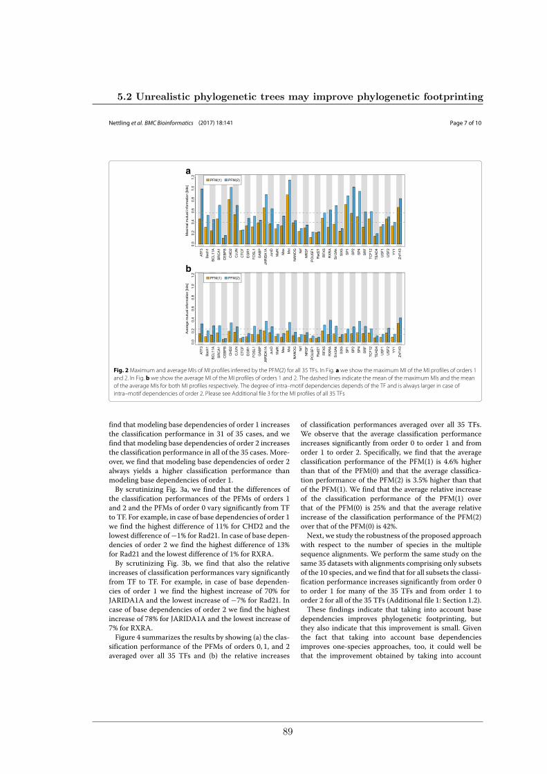
Nettling et al. BMC Bioinformatics (2017) 18:141 Page 7 of 10

a

b

Fig. 2Maximum and average MIs of MI profiles inferred by the PFM(2) for all 35 TFs. In Fig. a we show the maximumMI of the MI profiles of orders 1and 2. In Fig. b we show the average MI of the MI profiles of orders 1 and 2. The dashed lines indicate the mean of the maximumMIs and the meanof the average MIs for both MI profiles respectively. The degree of intra–motif dependencies depends of the TF and is always larger in case ofintra–motif dependencies of order 2. Please see Additional file 3 for the MI profiles of all 35 TFs

find that modeling base dependencies of order 1 increasesthe classification performance in 31 of 35 cases, and wefind that modeling base dependencies of order 2 increasesthe classification performance in all of the 35 cases. More-over, we find that modeling base dependencies of order 2always yields a higher classification performance thanmodeling base dependencies of order 1.By scrutinizing Fig. 3a, we find that the differences of

the classification performances of the PFMs of orders 1and 2 and the PFMs of order 0 vary significantly from TFto TF. For example, in case of base dependencies of order 1we find the highest difference of 11% for CHD2 and thelowest difference of−1% for Rad21. In case of base depen-dencies of order 2 we find the highest difference of 13%for Rad21 and the lowest difference of 1% for RXRA.By scrutinizing Fig. 3b, we find that also the relative

increases of classification performances vary significantlyfrom TF to TF. For example, in case of base dependen-cies of order 1 we find the highest increase of 70% forJARIDA1A and the lowest increase of −7% for Rad21. Incase of base dependencies of order 2 we find the highestincrease of 78% for JARIDA1A and the lowest increase of7% for RXRA.Figure 4 summarizes the results by showing (a) the clas-

sification performance of the PFMs of orders 0, 1, and 2averaged over all 35 TFs and (b) the relative increases

of classification performances averaged over all 35 TFs.We observe that the average classification performanceincreases significantly from order 0 to order 1 and fromorder 1 to order 2. Specifically, we find that the averageclassification performance of the PFM(1) is 4.6% higherthan that of the PFM(0) and that the average classifica-tion performance of the PFM(2) is 3.5% higher than thatof the PFM(1). We find that the average relative increaseof the classification performance of the PFM(1) overthat of the PFM(0) is 25% and that the average relativeincrease of the classification performance of the PFM(2)over that of the PFM(0) is 42%.Next, we study the robustness of the proposed approach

with respect to the number of species in the multiplesequence alignments. We perform the same study on thesame 35 datasets with alignments comprising only subsetsof the 10 species, and we find that for all subsets the classi-fication performance increases significantly from order 0to order 1 for many of the 35 TFs and from order 1 toorder 2 for all of the 35 TFs (Additional file 1: Section 1.2).These findings indicate that taking into account base

dependencies improves phylogenetic footprinting, butthey also indicate that this improvement is small. Giventhe fact that taking into account base dependenciesimproves one-species approaches, too, it could well bethat the improvement obtained by taking into account

5.2 Unrealistic phylogenetic trees may improve phylogenetic footprinting

89

Page 100

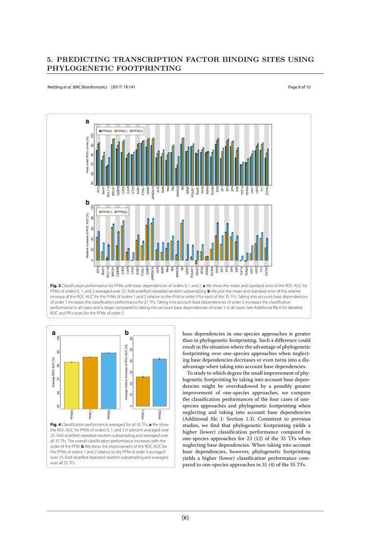
Nettling et al. BMC Bioinformatics (2017) 18:141 Page 8 of 10

a

b

Fig. 3 Classification performance for PFMs with base dependencies of orders 0, 1 and 2. aWe show the mean and standard error of the ROC AUC forPFMs of orders 0, 1, and 2 averaged over 25–fold stratified repeated random subsampling. bWe plot the mean and standard error of the relativeincrease of the ROC AUC for the PFMs of orders 1 and 2 relative to the PFM or order 0 for each of the 35 TFs. Taking into account base dependenciesof order 1 increases the classification performance for 31 TFs. Taking into account base dependencies of order 2 increases the classificationperformance in all cases and is larger compared to taking into account base dependencies of order 1 in all cases. See Additional file 6 for detailedROC and PR curves for the PFMs of order 2

a b

Fig. 4 Classification performance averaged for all 35 TFs. aWe showthe ROC AUC for PFMs of orders 0, 1, and 2 in percent averaged over25–fold stratified repeated random subsampling and averaged overall 35 TFs. The overall classification performance increases with theorder of the PFM. bWe show the improvement of the ROC AUC forthe PFMs of orders 1 and 2 relative to the PFM of order 0 averagedover 25–fold stratified repeated random subsampling and averagedover all 35 TFs

base dependencies in one-species approaches is greaterthan in phylogenetic footprinting. Such a difference couldresult in the situation where the advantage of phylogeneticfootprinting over one-species approaches when neglect-ing base dependencies decreases or even turns into a dis-advantage when taking into account base dependencies.To study to which degree the small improvement of phy-

logenetic footprinting by taking into account base depen-dencies might be overshadowed by a possibly greaterimprovement of one-species approaches, we comparethe classification performances of the four cases of one-species approaches and phylogenetic footprinting whenneglecting and taking into account base dependencies(Additional file 1: Section 1.3). Consistent to previousstudies, we find that phylogenetic footprinting yields ahigher (lower) classification performance compared toone-species approaches for 23 (12) of the 35 TFs whenneglecting base dependencies. When taking into accountbase dependencies, however, phylogenetic footprintingyields a higher (lower) classification performance com-pared to one-species approaches in 31 (4) of the 35 TFs.

5. PREDICTING TRANSCRIPTION FACTOR BINDING SITES USINGPHYLOGENETIC FOOTPRINTING

90

Page 101

Nettling et al. BMC Bioinformatics (2017) 18:141 Page 9 of 10

This finding indicates that the small improvement ofphylogenetic footprinting by taking into account basedependencies is greater than the corresponding improve-ment of one-species approaches. It also indicates that thepreviously observed advantage of phylogenetic footprint-ing over one-species approaches when neglecting basedependencies (23 to 12) does not decrease or turn intoa disadvantage, but becomes even more pronounced (31to 4), when taking into account base dependencies. Thisincreased advantage of phylogenetic footprinting overone-species approaches achieved by taking into accountbase dependencies is surprising as it indicates the pres-ence of some synergy of modeling both phylogenetic andbase dependencies.We finally study for each of the 35 TFs which of

the four models yields the highest classification perfor-mance, and we find that one-species approaches neglect-ing base dependencies yields the highest classificationperformance for one TF (CEBPB), one-species approachestaking into account base dependencies yields the high-est classification performance for three TFs (BCL11A,MafK, and RXRA), phylogenetic footprinting neglectingbase dependencies never yields the highest classificationperformance, and phylogenetic footprinting taking intoaccount base dependencies yields the highest classifica-tion performance for 31 TFs. This finding indicates thatphylogenetic footprinting can be improved by taking intoaccount base dependencies, that one-species approachesusing base dependencies can be improved by taking intoaccount phylogenetic dependencies, and that there is asurprising synergy of simultaneously modeling both phy-logenetic and base dependencies.

ConclusionsIn this work, we introduced a phylogenetic footprintingmodel capable of taking into account base dependen-cies and evaluated this phylogenetic footprinting modelon ChIP-seq data of 35 TFs. We found significant intra-motif dependencies of orders 1 and 2 in all 35 datasetsand that the inferred intra-motif dependencies of order2 are stronger than those of order 1 for all 35 TFs. Wealso found that these intra-motif dependencies cannotbe explained as an artifact resulting from a mixture ofdifferent species-specific motifs. We further found thatthe classification performance of the introduced phyloge-netic footprinting model is higher than that of phyloge-netic footprinting models neglecting base dependenciesfor all of the 35 TFs and higher than that of one-speciesapproaches for 31 of the 35 TFs. These findings sug-gest that combining phylogenetic footprinting with motifmodels incorporating intra-motif dependencies may leadto an improved prediction of TFBSs and thus advance ourunderstanding of transcriptional gene regulation and itsevolution.

Additional files

Additional file 1: Supplementary Material. This file is structured in threesections, presenting four additional studies, details about theimplementation and some statistics regarding the datasets of all 35 TFs.In Section 1, Supplementary Results, we first study differences amongspecies–specific motifs of 35 TFs. We then study the robustness of theproposed PFM to different species compositions on data of 35 TFs. Third,we examine the impact of base dependencies and phylogeneticdependencies on classification performance. In the fourth subsection, wecompare the proposed PFM(2) with a state of the art tool by Eggeling et al.2015 [13] on data of 35 TFs. In the fifth subsection, we show statistics of thedistances between ChIP-seq positive regions and the alignment coverageof ten species. Finally, we specify the run–time of our freely availableimplementation of the proposed PFM.In Section 2, Supplementary Methods, we specify details about theestimation of species–specific motifs and we define a statistical test for thesignificance of differences among species–specific motifs.In Section 3, Supplementary Tables, we show statistics of the datasets of 35TFs, summarize results regarding the significance of species–specific motifsand the impact of base dependencies and phylogenetic dependencies, andshow the alignment coverage of ten species for 35 TFs. (PDF 1034.24 kb)

Additional file 2: Sequence data. This archive contains data files ofalignments of the ChIP-seq positive regions and negative control regionsfor each of the 35 TFs in FASTA format. (ZIP 83763.2 kb)

Additional file 3: Sequence logos, MI profiles of order 1, MI profiles oforder 2, and species-specific MI profiles of orders 1 and 2. The file containsfor each of the 35 TFs the sequence logo inferred using the PFM(2) alignedwith MI profiles of order 1, the MI profiles of order 2, and species-specific MIprofiles of orders 1 and 2 for each of the 10 species. (PDF 2129.92 kb)

Additional file 4: Tables of difference logos. The file contains for each ofthe 35 TFs a 10 × 10 table of difference logos for a pair-wise visualcomparison of species-specific motifs. (ZIP 26112 kb)

Additional file 5: Sequence logos of predicted binding sites. The filecontains sequence logos and their reverse complements of predictedbinding sites inferred using the PFM(0), the PFM(1), and the PFM(2) foreach of the 35 TFs. (PDF 11776 kb)

Additional file 6: ROC curves. The pdf file comprises for each TF one plotthat shows the 25 ROC curves and one plot that shows the 25 PR curvesfrom the 25–fold stratified repeated random sub-sampling validationprocedure described in Methods 3. (PDF 2611.2 kb)

AbbreviationsMI: mutual information; PFM: phylogenetic footprinting model; PWM: positionweight matrix; TF: transcription factor; TFBS: transcription factor binding site

Authors’ contributionsMN and IG developed the key idea. MN and JC developed the computationalmethods. MN and HT performed the studies. All authors wrote, read, andapproved the final manuscript.

AcknowledgementsWe thank Ralf Eggeling, Jan Grau, Patrice Peterson, and Marcel Quint forvaluable discussions. We thank the HudsonAlpha Institute for Biotechnology,the Stanford University, the Broad Institute of MIT and Harvard, and theUniversity of Southern California for performing the ChIP-seq experiments andthe ENCODE Analysis Working Group for providing the datasets.

FundingThis work was financially supported by DFG (grant no. GR3526/1), Gencat(2014 SGR 118), and Collectiveware (TIN2015-66863-C2-1-R).

Availability of data andmaterialsThe datasets used in this work are included within the article and its additionalfiles. The implementation of the proposed phylogenetic footprinting model isavailable at https://github.com/mgledi/PhyFoo/.

5.2 Unrealistic phylogenetic trees may improve phylogenetic footprinting

91

Page 102

Nettling et al. BMC Bioinformatics (2017) 18:141 Page 10 of 10

Competing interestsThe authors declare that they have no competing interests.

Consent for publicationNot applicable.

Ethics approval and consent to participateNot applicable.

Author details1Institute of Computer Science, Martin Luther University Halle-Wittenberg,Halle, Germany. 2Leibniz Institute of Plant Biochemistry, Halle, Germany.3Institut d’Investigació en Intel·ligència Artificial, IIIA-CSIC, Campus UAB,Cerdanyola, Spain. 4German Centre for Integrative Biodiversity Research (iDiv)Halle-Jena-Leipzig, Leipzig, Germany.

Received: 29 June 2016 Accepted: 24 January 2017

References1. Smith ZD, Meissner A. DNA methylation: roles in mammalian

development. Nat Rev Genet. 2013;14(3):204–20. doi:10.1038/nrg3354.2. Tessarz P, Kouzarides T. Histone core modifications regulating

nucleosome structure and dynamics. Nat Rev Mol Cell Biol. 2014;15(11):703–8. doi:10.1038/nrm3890.

3. Sainsbury S, Bernecky C, Cramer P. Structural basis of transcriptioninitiation by RNA polymerase II. Nat Rev Mol Cell Biol. 2015;16(3):129–43.doi:10.1038/nrm3952.

4. Schoenberg DR, Maquat LE. Regulation of cytoplasmic mRNA decay.Nat Rev Genet. 2012;13(4):246–59. doi:10.1038/nrg3160.

5. de Fougerolles A, Vornlocher HP, Maraganore J, Lieberman J. Interferingwith disease: a progress report on sirna-based therapeutics. Nat Rev DrugDiscov. 2007;6(6):443–53.

6. Tam OH, Aravin AA, Stein P, Girard A, Murchison EP, Cheloufi S, HodgesE, Anger M, Sachidanandam R, Schultz RM, et al. Pseudogene-derivedsmall interfering rnas regulate gene expression in mouse oocytes. Nature.2008;453(7194):534–8.

7. Sultan M, Schulz MH, Richard H, Magen A, Klingenhoff A, Scherf M,Seifert M, Borodina T, Soldatov A, Parkhomchuk D, et al. A global view ofgene activity and alternative splicing by deep sequencing of the humantranscriptome. Science. 2008;321(5891):956–60.

8. Luco RF, Pan Q, Tominaga K, Blencowe BJ, Pereira-Smith OM, Misteli T.Regulation of alternative splicing by histone modifications. Science.2010;327(5968):996–1000.

9. Hobert O. Gene regulation by transcription factors and micrornas.Science. 2008;319(5871):1785–6.

10. Voss TC, Hager GL. Dynamic regulation of transcriptional states bychromatin and transcription factors. Nat Rev Genet. 2014;15(2):69–81.

11. Bulyk ML, Johnson PL, Church GM. Nucleotides of transcription factorbinding sites exert interdependent effects on the binding affinities oftranscription factors. Nucleic Acids Res. 2002;30(5):1255–61.

12. Salama RA, Stekel DJ. Inclusion of neighboring base interdependenciessubstantially improves genome-wide prokaryotic transcription factorbinding site prediction. Nucleic Acids Res. 2010;38(12):135–5.

13. Eggeling R, Roos T, Myllymäki P, Grosse I. Inferring intra-motifdependencies of dna binding sites from chip-seq data. BMC Bioinforma.2015;16(1):375.

14. Grau J, Posch S, Grosse I, Keilwagen J. A general approach fordiscriminative de novo motif discovery from high-throughput data.Nucleic Acids Res. 2013;41(21):e197. doi:10.1093/nar/gkt831.

15. Ma W, Noble WS, Bailey TL. Motif-based analysis of large nucleotide datasets using meme-chip. Nat Protoc. 2014;9(6):1428–50.

16. Alipanahi B, Delong A, Weirauch MT, Frey BJ. Predicting the sequencespecificities of DNA- and RNA-binding proteins by deep learning.Nat Biotechnol. 2015;33(8):831–8. doi:10.1038/nbt.3300.

17. Kulakovskiy I, Levitsky V, Oshchepkov D, Bryzgalov L, Vorontsov I,Makeev V. From binding motifs in chip-seq data to improved models oftranscription factor binding sites. J Bioinforma Comput Biol. 2013;11(01):1340004.

18. Felsenstein J. Evolutionary trees from DNA sequences: a maximumlikelihood approach. J Mol Evol. 1981;17(6):368–76.

19. Schmidt D, Wilson MD, Ballester B, Schwalie PC, Brown GD, Marshall A,Kutter C, Watt S, Martinez-Jimenez CP, Mackay S, Talianidis I, Flicek P,Odom DT. Five-vertebrate ChIP-seq reveals the evolutionary dynamics oftranscription factor binding. Sci (New York, NY). 2010;328(5981):1036–40.doi:10.1126/science.1186176.

20. Hardison RC, Taylor J. Genomic approaches towards findingcis-regulatory modules in animals. Nat Rev Genet. 2012;13(7):469–83.

21. Katara P, Grover A, Sharma V. Phylogenetic footprinting: a boost formicrobial regulatory genomics. Protoplasma. 2012;249(4):901–7.

22. Martinez-Morales JR. Toward understanding the evolution of vertebrategene regulatory networks: comparative genomics and epigenomicapproaches. Brief Funct Genom. 2015. doi:10.1093/bfgp/elv032.

23. Blanchette M, Tompa M. Footprinter: a program designed forphylogenetic footprinting. Nucleic Acids Res. 2003;31(13):3840–2.

24. Sinha S, Blanchette M, Tompa M. Phyme: a probabilistic algorithm forfinding motifs in sets of orthologous sequences. BMC Bioinforma.2004;5(1):170.

25. Moses A, Chiang D, Pollard D, Iyer V, Eisen M. Monkey: identifyingconserved transcription-factor binding sites in multiple alignments usinga binding site-specific evolutionary model. Genome Biol. 2004;5(12):98.doi:10.1186/gb-2004-5-12-r98.

26. Neph S, Tompa M. Microfootprinter: a tool for phylogenetic footprintingin prokaryotic genomes. Nucleic Acids Res. 2006;34(suppl 2):366–8.

27. Newberg LA, Thompson WA, Conlan S, Smith TM, McCue LA,Lawrence CE. A phylogenetic gibbs sampler that yields centroid solutionsfor cis-regulatory site prediction. Bioinformatics. 2007;23(14):1718–27.

28. Siddharthan R, Siggia ED, Van Nimwegen E. Phylogibbs: a gibbs samplingmotif finder that incorporates phylogeny. PLoS Comput Biol. 2005;1(7):67.

29. Siddharthan R. Phylogibbs-mp: module prediction and discriminativemotif-finding by gibbs sampling. PLoS Comput Biol. 2008;4(8):1000156.

30. Arnold P, Erb I, Pachkov M, Molina N, van Nimwegen E. Motevo:integrated bayesian probabilistic methods for inferring regulatory sitesand motifs on multiple alignments of dna sequences. Bioinformatics.2012;28(4):487–94. doi:10.1093/bioinformatics/btr695.

31. ENCODE Project Consortium. An integrated encyclopedia of DNAelements in the human genome. Nature. 2012;489(7414):57–74.doi:10.1038/nature11247.

32. UCSC. Genome Bioinformatics. 2016. http://hgdownload.cse.ucsc.edu/downloads.html. Accessed 29 Apr 2016.

33. Landt SG, Marinov GK, Kundaje A, Kheradpour P, Pauli F, Batzoglou S,Bernstein BE, Bickel P, Brown JB, Cayting P, et al. Chip-seq guidelines andpractices of the encode and modencode consortia. Genome Res.2012;22(9):1813–31.

34. Kharchenko PV, Tolstorukov MY, Park PJ. Design and analysis of ChIP-seqexperiments for DNA-binding proteins. Nat Biotech. 2008;26(12):1351–9.doi:10.1038/nbt.1508.

35. ENCODE. Uniform TFBS composite track. http://hgdownload.cse.ucsc.edu/goldenpath/hg19/encodeDCC/wgEncodeAwgTfbsUniform/.Accessed 29 Apr 2016.

36. Multiple alignments of the hg19/GRCh37 human genome assembly.http://hgdownload.cse.ucsc.edu/goldenPath/hg19/multiz46way/.Accessed 29 Apr 2016.

37. Lawrence CE, Altschul SF, Boguski MS, Liu JS, Neuwald AF, Wootton JC.Detecting subtle sequence signals: a gibbs sampling strategy for multiplealignment. Science. 1993;262(5131):208–14.

38. Redhead E, Bailey TL. Discriminative motif discovery in dna and proteinsequences using the deme algorithm. BMC Bioinforma. 2007;8(1):1.

39. Keilwagen J, Grau J, Paponov IA, Posch S, Strickert M, Grosse I. De-novodiscovery of differentially abundant transcription factor binding sitesincluding their positional preference. PLoS Comput Biol. 2011;7(2):1001070.

40. Agostini F, Cirillo D, Ponti RD, Tartaglia GG. Seamote: a method forhigh-throughput motif discovery in nucleic acid sequences. BMCGenomics. 2014;15(1):925.

41. Lawrence CE, Reilly AA. An expectation maximization (em) algorithm forthe identification and characterization of common sites in unalignedbiopolymer sequences. Proteins Struct Funct Bioinforma. 1990;7(1):41–51.

42. Grau J, Keilwagen J, Gohr A, Haldemann B, Posch S, Grosse I. Jstacs: ajava framework for statistical analysis and classification of biologicalsequences. J Mach Learn Res. 2012;13(1):1967–71.

5. PREDICTING TRANSCRIPTION FACTOR BINDING SITES USINGPHYLOGENETIC FOOTPRINTING

92

Page 103

5.3 Combining phylogenetic footprinting with motif models incorporatingintra-motif dependencies

5.3 Combining phylogenetic footprinting with motif modelsincorporating intra-motif dependencies

M Nettling, H Treutler, J Cerquides, I Grosse. 2017. Combining phylogenetic foot-printing with motif models incorporating intra-motif dependencies. BMC Bioinformatics,18:141 doi: 0.1186/s12859-017-1495-1

93

Page 104

Phlogenetics

Unrealistic phylogenetic trees may improve

phylogenetic footprinting

Martin Nettling1,*, Hendrik Treutler2, Jesus Cerquides3 and

Ivo Grosse1,4

1Institute of Computer Science, Martin Luther University Halle-Wittenberg, Halle, Germany, 2Department of Stress

and Developmental Biology, Leibniz Institute of Plant Biochemistry, Halle, Germany, 3Institut d’Investigaci�o en Intel

ligencia Artificial, IIIA-CSIC, Campus UAB, Cerdanyola, Spain and 4German Centre for Integrative Biodiversity

Research (iDiv) Halle-Jena-Leipzig, Leipzig, Germany

*To whom correspondence should be addressed.

Associate Editor: Janet Kelso

Received on March 2, 2016; revised on December 2, 2016; editorial decision on January 18, 2017; accepted on January 19, 2017

Abstract

Motivation: The computational investigation of DNA binding motifs from binding sites is one of the

classic tasks in bioinformatics and a prerequisite for understanding gene regulation as a whole. Due

to the development of sequencing technologies and the increasing number of available genomes,

approaches based on phylogenetic footprinting become increasingly attractive. Phylogenetic foot-

printing requires phylogenetic trees with attached substitution probabilities for quantifying the evolu-

tion of binding sites, but these trees and substitution probabilities are typically not known and cannot

be estimated easily.

Results: Here, we investigate the influence of phylogenetic trees with different substitution proba-

bilities on the classification performance of phylogenetic footprinting using synthetic and real data.

For synthetic data we find that the classification performance is highest when the substitution prob-

ability used for phylogenetic footprinting is similar to that used for data generation. For real data,

however, we typically find that the classification performance of phylogenetic footprinting surpris-

ingly increases with increasing substitution probabilities and is often highest for unrealistically

high substitution probabilities close to one. This finding suggests that choosing realistic model as-

sumptions might not always yield optimal predictions in general and that choosing unrealistically

high substitution probabilities close to one might actually improve the classification performance

of phylogenetic footprinting.

Availability and Implementation: The proposed PF is implemented in JAVA and can be down-

loaded from https://github.com/mgledi/PhyFoo

Contact: [email protected]

Supplementary information: Supplementary data are available at Bioinformatics online.

1 Introduction

Gene regulation is a highly complex process in nature based on sev-

eral sub-processes such as transcriptional regulation including DNA

methylation (Smith and Meissner, 2013), histone modifications

(Tessarz and Kouzarides, 2014) and promotor escaping (Sainsbury

et al., 2015) as well as post-transcriptional regulation including

modulated mRNA decay (Schoenberg and Maquat, 2012), siRNA

interference (de Fougerolles et al., 2007; Tam et al., 2008) and al-

ternative splicing (Luco et al., 2010; Sultan et al., 2008). One im-

portant step in this complex process is the regulation of

transcriptional initiation by the interaction of transcription factors

(TFs) with their binding sites (Hobert, 2008; Voss and Hager,

2014). Hence, identifying transcription factor binding sites (TFBSs)

and inferring their binding motifs is a prerequisite in modern

VC The Author 2017. Published by Oxford University Press. 1

This is an Open Access article distributed under the terms of the Creative Commons Attribution Non-Commercial License (http://creativecommons.org/licenses/by-nc/4.0/),

which permits non-commercial re-use, distribution, and reproduction in any medium, provided the original work is properly cited. For commercial re-use, please contact

[email protected]

Bioinformatics, 2017, 1–8

doi: 10.1093/bioinformatics/btx033

Advance Access Publication Date: 27 January 2017

Original Paper

5. PREDICTING TRANSCRIPTION FACTOR BINDING SITES USINGPHYLOGENETIC FOOTPRINTING

94

Page 105

biology, medicine and biodiversity research (Nowrousian, 2010;

Villar et al., 2014).

The last decade has witnessed a spectacular development of

sequencing technologies unleashing new potentials in identifying

TFBSs (Kulakovskiy et al., 2010; Furey, 2012; Lasken and McLean,

2014; van Dijk et al., 2016). Due to the increasing number of avail-

able genomes of different species and due to increasing computa-

tional resources, approaches for de-novo motif discovery based on

phylogenetic footprinting have become increasingly attractive.

Examples of highly popular tools for phylogenetic footprinting are

FootPrinter (Blanchette and Tompa, 2003), PhyME (Sinha et al.,

2004), MONKEY (Moses et al., 2004a), PhyloGibbs (Siddharthan

et al., 2005), Phylogenetic Gibbs Sampler (Newberg et al., 2007),

PhyloGibbs-MP (Siddharthan, 2008) and MotEvo (Arnold et al.,

2012). Supplementary Table S1 provides a comparison of these tools

regarding the used evolutionary model, sequence model and learning

principle.

One prerequisite for most phylogenetic footprinting approaches

are multiple sequence alignments (MSAs) of upstream regions of

orthologous genes of multiple not too closely related species

(Anisimova et al., 2013). These MSAs capture phylogenetic infor-

mation, and the key idea of using these MSAs as starting point for

phylogenetic footprinting results from the observations that (i) func-

tional TFBSs are phylogenetically conserved and (ii) phylogenetic-

ally conserved TFBSs are aligned in MSAs. Examples of highly

popular tools for aligning non-coding genomic regions are T-Coffee

(Notredame et al., 2000), WebPRANK (Loytynoja and Goldman,

2010) and MAFFT (Katoh and Standley, 2013).

Phylogenetic footprinting improves the de-novo motif discovery

by incorporating phylogenetic dependencies within the MSA in con-

trast to approaches based on sequences from only one species.

Substitution models of DNA sequence evolution such as the F81

model (Felsenstein, 1981) have been adapted to model the evolution

of TFBSs in a position-specific manner, and it has been shown that

these adapted models, which we call phylogenetic footprinting mod-

els (PFMs) for brevity, can detect TFBSs more accurately than mod-

els that neglect phylogenetic dependencies (Clark et al., 2007; Gertz

et al., 2006; Hardison and Taylor, 2012; Hawkins et al., 2009;

Moses et al., 2004a; Nettling et al., 2017).

One fundamental prerequisite for phylogenetic footprinting is a

phylogenetic tree including substitution probabilities attached to

each of its branches, and choosing an appropriate phylogenetic tree

and appropriate substitution probabilities is pivotal for the classifi-

cation performance of phylogenetic footprinting (Kc and Livesay,

2011). However, estimating substitution probabilities within TFBSs

is substantially harder than estimating them e.g. in protein-coding

regions for at least two reasons:

First, the positions of TFBSs are unknown when performing

phylogenetic footprinting, whereas the positions of protein-coding

regions are known when estimating substitution probabilities there.

Second, protein-coding regions are much longer than TFBSs, so one

can use a much larger number of bases for estimating substitution

probabilities for protein-coding regions than for TFBSs.

Estimating substitution probabilities within TFBSs is challeng-

ing, but several valuable studies have been performed in this direc-

tion (Doniger and Fay, 2007; Pollard et al., 2010; Schaefke et al.,

2015; Tu�grul et al., 2015). For example, studies on synthetic data

have indicated that small substitution probabilities in the motif and

moderate substitution probabilities in the flanking sequences can be

preferable for motif recognition (Sinha et al., 2004), and studies on

different yeast species have confirmed these findings and shown that

the likelihood of the Jukes-Cantor model (Jukes and Cantor, 1969)

increases relative to a thymine background (‘polyT’) for small sub-

stitution probabilities in the motif and moderate substitution proba-

bilities in the flanking sequences (Moses et al., 2004b).

These and similar findings, however, have not lead to a robust

approach of estimating substitution probabilities within TFBSs prior

to or as part of phylogenetic footprinting, so the substitution proba-

bilities are often simply taken from the literature or guessed, and

their influence on the classification performance of phylogenetic

footprinting has not yet been studied systematically.

Here, we study this influence based on a synthetic dataset and

five real datasets of the TFs CTCF, GABP, NRSF, SRF and STAT1.

Specifically, we describe the PFM, the datasets, the tested phylogen-

etic trees, the performance measure, and implementation details in

section Methods, and we study the classification performance of

phylogenetic footprinting as a function of the substitution rate for

synthetic and real datasets, compare the results to those of phylogen-

etic footprinting based on expert trees from the literature, and dis-

cuss the findings in the context of several factors that affect the

evolution of TFBSs in sections 3 and 4.

2 Materials and methods

In this section we describe (i) the used notation and the likelihood

calculation of the PFM, (ii) the investigated datasets, (iii) the per-

formance measure, (iv) the systematic investigation of phylogenetic

trees and (v) the implementation of the PFMs.

2.1 Phylogenetic footprinting model2.1.1 Notation

Our data contains N alignments, with each alignment containing O

sequences (one per observed species) of length Ln.

Our phylogenetic model incorporates the existence of H add-

itional hidden species, that is, species for which we cannot observe

their sequences. Both hidden and observed species conform a tree.

Thus, for each species k but the root, pa(k) denotes the ancestor of

species k in the tree. The root species is noted r.

Our probabilistic model contains a random variable Su;kn for each

nucleotide 1 � u � Ln of each species 1 � k � OþH of each

alignment 1 � n � N. These random variables take values in the

set of bases A ¼ fA;C;G;Tg. We note paðSu;kn Þ the uth nucleotide in

the nth alignment of species pa(k) (the ancestor of k). By definition,

the root has no ancestor and hence paðSu;rn Þ ¼1. We also refer to

nucleotide Su;kn as Au;k

n when species k is observed, and as Yu;kn when

species k is hidden. Furthermore we note by Yu;:n (respectively Su;:

n )

the set containing each random variable Yu;kn (respectively Su;k

n ), with

Oþ 1 � k � OþH and Yn the set containing every random vari-

able in Yu;:n with 1 � u � Ln:

An alignment An may or may not contain a TFBS. This is

encoded in variable Mn, with M0n indicating that alignment An does

not contain a motif and M1n indicating that alignment An does con-

tain a motif.

2.1.2 Likelihood

The probability that the alignment An is generated by the PFM can

be written as

pðAnjhÞ ¼ pðAnjM0n; hÞ � pðM0

njhÞ þ pðAnjM1n; hÞ � pðM1

njhÞ

with variable Mn taking a Bernoulli distribution and h denoting

model parameters, namely the topology of the phylogenetic tree, the

substitution probabilities and the evolutionary model with its

2 M.Nettling et al.

5.3 Combining phylogenetic footprinting with motif models incorporatingintra-motif dependencies

95

Page 106

stationary probabilities for the flanking regions as well as the TFBS

regions.

We need to specify the probability for non-motif-bearing pðAnjM0

n; hÞ and for motif-bearing alignments pðAnjM1n; hÞ. For reasons of

clarity we omit h in the following.

2.1.3 Likelihood of a non-motif-bearing alignment

The probability that alignment An is generated by the PFM as a non-

motif bearing alignment is

pðAnjM0nÞ ¼

XYn

pðAnjYn;M0nÞ: (1)

We assume that each single nucleotide alignment is independent

of any other nucleotide alignment given h and M0n. Furthermore, we

assume that in each nucleotide alignment, the species satisfy the con-

ditional independencies encoded by the phylogenetic tree. Thus,

pðAnjM0nÞ ¼

QLn

u¼1

PYu;:

npðSu;:

n jM0nÞ (2)

¼QLn

u¼1

PYu;:

n

QOþHk¼1 pðSu;k

n jpaðSu;kn Þ;M0

nÞ (3)

where

pðSu;kn ¼ ajpaðSu;k

n Þ ¼ b;M0nÞ ¼

pa0 if k ¼ r

ck � pa0 þ ð1� ckÞda¼b if k 6¼ r

(

according to the F81 model, where the base distribution of each pos-

ition of the background sequence is denoted by p0, the probability

of a nucleotide a in the background sequence is denoted by pa0, and

the substitution probability from the ancestor species to species k is

denoted by ck. For more realistic phylogenetic models ck might also

depend on specific nucleotide transitions.

2.1.4 Likelihood of a motif-bearing alignment

The probability that alignment An is generated by the PFM as a

motif bearing alignment is

pðAnjM1nÞ ¼

XLn�Wþ1

‘n¼1

XYn

pðAn;Yn; ‘njM1nÞ: (4)

where W is the length of the TFBS and ‘n is the position of the TFBS

in alignment An. Since single nucleotide alignments are assumed in-

dependent and considering the conditional independencies in the

phylogenetic tree we have

pðAnjM1nÞ ¼

XLn�Wþ1

‘n¼1

pð‘njM1nÞYLn

u¼1

XYu;:

n

pðSu;:n j‘n;M

1nÞ (5)

with pðSu;:n j‘n;M1

nÞ ¼QOþH

k¼1 pðSu;kn jpaðSu;k

n Þ; ‘n;M1nÞ and

pðSu;kn jpaðSu;k

n Þ;‘n;M1nÞ

¼

pa0 if k¼ r and u< ‘n or u� ‘nþW

pau�‘nþ1 if k¼ r and ‘n � u< ‘nþW

ck�pa0þð1�ckÞda¼b if k 6¼ r and u< ‘n or u� ‘nþW

ck�pau�‘nþ1þð1�ckÞda¼b if k 6¼ r and ‘n � u< ‘nþW

8>>>>>><>>>>>>:

As for the non-motif-bearing alignment, the base distribution of

each position of the background sequence is denoted by p0 and the

probability of a nucleotide a in the background sequence is denoted by

pa0. The base distributions of a motif sequence of length W are denoted

by pw with w 2 ½1; . . . ;W� and the probability of a nucleotide a at

position w in a motif sequence is denoted by paw. The substitution

probability from the ancestor species to species k is denoted by ck.

Finally we assume motifs to be uniformly distributed, thus hav-

ing that pð‘njM1nÞ ¼ 1

Ln�Wþ1, which completes the specification of

the likelihood function.

2.2 Data2.2.1 Real data

The data used in this work originate from human ChIP-Seq data of

the five TFs CTCF, GABP, NRSF, SRF and STAT1 Jothi et al. (2008);

Valouev et al. (2008) and gapped alignments of the ChIP-Seq target

regions from human with orthologous regions from monkey, cow,

dog and horse. The original data provided by Arnold et al. (2012)

consist of 900 gapped alignments for each of the five TFs. Each

gapped alignment consists of sequences from six species. Since gapped

alignments have a higher risk of showing mathematical side effects,

we process them to derive ungapped alignments following three steps:

(i) We remove the species that causes the highest number of gaps in all

alignments. Accordingly, we remove sequences from opossum and

keep orthologous regions from human, monkey, cow, dog and horse.

(ii) In each alignment, we remove all alignment columns that contain

at least one gap. (iii) We remove all alignments that are shorter than

21bp, which is the length of the longest TFBS motif (NRSF) in the

presented studies. Supplementary Table S2 shows details about the re-

sulting datasets. All datasets are available as Supplementary Material.

2.2.2 Synthetic data

The synthetic dataset used in this work is generated using the PFM

specified in section 2.1 with a star topology.

A negative set of 1000 non-motif-bearing alignments each of

length L ¼ 300 is generated. Each non-motif bearing alignment is

generated in two steps as follows. (i) Sample the primordial se-

quence. For each position u 2 ½1;L� of the sequence, sample a nu-

cleotide from the uniform distribution p0. (ii) For each of the

descent species o 2 f1; . . . ;5g, sample a mutated sequence given the

primordial sequence position-wise. For each position u 2 ½1;L�,apply the F81 Felsenstein (1981) mutation model with the equilib-

rium distribution p0 and substitution probability c ¼ 0:2 to the nu-

cleotide of the primordial sequence at position u.

A positive set of 750 motif-bearing alignments each of length

L ¼ 300 is generated. Each motif-bearing alignment is generated as

follows:

(i) Sample the primordial sequence given a TFBS length of W ¼ 15.

(a) Sample the start position ‘ 2 ½1;L�W þ 1� of the TFBS

from the uniform distribution.

(b) For each position u 2 ½1; ‘� 1� and u 2 ½‘þW;L� of the

flanking sequence, we sample the nucleotide at position u

from the uniform distribution p0. For each position

u 2 ½‘; ‘þW � 1� of the TFBS, we sample the nucleotide

at position u from the distribution pu�‘nþ1. The distribu-

tion pw with w 2 f1; . . . ; 15g is uniformly drawn from the

simplex.

(ii) For each of the descent species o 2 f1; . . . ; 5g, sample a mutated

sequence given the primordial sequence position-wise.

(a) For each position u 2 ½1; ‘� 1� and u 2 ½‘þW;L� of the

flanking sequence, apply the F81 mutation model with the

equilibrium distribution p0 and substitution probability

c ¼ 0:2 to the nucleotide of the primordial sequence at

position u.

(b) For each position u 2 ½‘; ‘þW � 1� of the TFBS, apply the

F81 mutation model with the equilibrium distribution

pu�‘nþ1 and substitution probability c ¼ 0:2 to the nucleo-

tide of the primordial sequence at position u.

Unrealistic phylogenetic trees 3

5. PREDICTING TRANSCRIPTION FACTOR BINDING SITES USINGPHYLOGENETIC FOOTPRINTING

96

Page 107

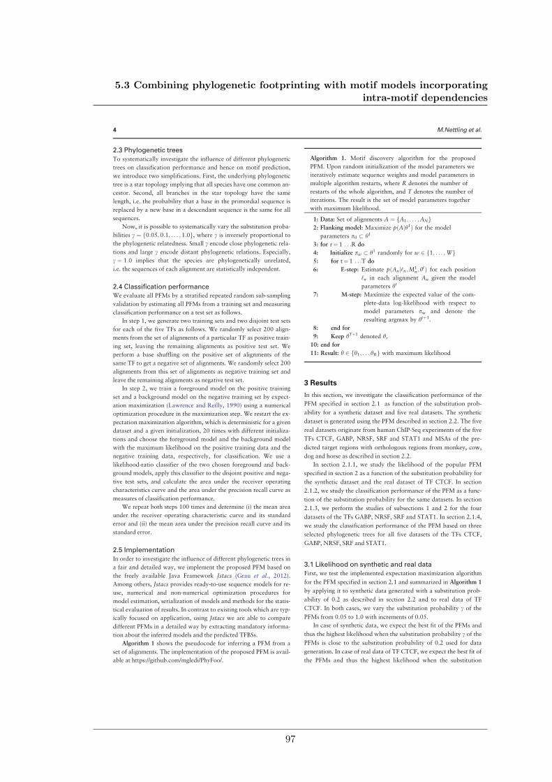
2.3 Phylogenetic treesTo systematically investigate the influence of different phylogenetic

trees on classification performance and hence on motif prediction,

we introduce two simplifications. First, the underlying phylogenetic

tree is a star topology implying that all species have one common an-

cestor. Second, all branches in the star topology have the same

length, i.e. the probability that a base in the primordial sequence is

replaced by a new base in a descendant sequence is the same for all

sequences.

Now, it is possible to systematically vary the substitution proba-

bilities c ¼ f0:05; 0:1; . . . ;1:0g, where c is inversely proportional to

the phylogenetic relatedness. Small c encode close phylogenetic rela-

tions and large c encode distant phylogenetic relations. Especially,

c ¼ 1:0 implies that the species are phylogenetically unrelated,

i.e. the sequences of each alignment are statistically independent.

2.4 Classification performanceWe evaluate all PFMs by a stratified repeated random sub-sampling

validation by estimating all PFMs from a training set and measuring

classification performance on a test set as follows.

In step 1, we generate two training sets and two disjoint test sets

for each of the five TFs as follows. We randomly select 200 align-

ments from the set of alignments of a particular TF as positive train-

ing set, leaving the remaining alignments as positive test set. We

perform a base shuffling on the positive set of alignments of the

same TF to get a negative set of alignments. We randomly select 200

alignments from this set of alignments as negative training set and

leave the remaining alignments as negative test set.

In step 2, we train a foreground model on the positive training

set and a background model on the negative training set by expect-

ation maximization (Lawrence and Reilly, 1990) using a numerical

optimization procedure in the maximization step. We restart the ex-

pectation maximization algorithm, which is deterministic for a given

dataset and a given initialization, 20 times with different initializa-

tions and choose the foreground model and the background model

with the maximum likelihood on the positive training data and the

negative training data, respectively, for classification. We use a

likelihood-ratio classifier of the two chosen foreground and back-

ground models, apply this classifier to the disjoint positive and nega-

tive test sets, and calculate the area under the receiver operating

characteristics curve and the area under the precision recall curve as

measures of classification performance.

We repeat both steps 100 times and determine (i) the mean area

under the receiver operating characteristic curve and its standard

error and (ii) the mean area under the precision recall curve and its

standard error.

2.5 ImplementationIn order to investigate the influence of different phylogenetic trees in

a fair and detailed way, we implement the proposed PFM based on

the freely available Java Framework Jstacs (Grau et al., 2012).

Among others, Jstacs provides ready-to-use sequence models for re-

use, numerical and non-numerical optimization procedures for

model estimation, serialization of models and methods for the statis-

tical evaluation of results. In contrast to existing tools which are typ-

ically focused on application, using Jstacs we are able to compare

different PFMs in a detailed way by extracting mandatory informa-

tion about the inferred models and the predicted TFBSs.

Algorithm 1 shows the pseudocode for inferring a PFM from a

set of alignments. The implementation of the proposed PFM is avail-

able at https://github.com/mgledi/PhyFoo/.

3 Results

In this section, we investigate the classification performance of the

PFM specified in section 2.1 as function of the substitution prob-

ability for a synthetic dataset and five real datasets. The synthetic

dataset is generated using the PFM described in section 2.2. The five

real datasets originate from human ChIP-Seq experiments of the five

TFs CTCF, GABP, NRSF, SRF and STAT1 and MSAs of the pre-

dicted target regions with orthologous regions from monkey, cow,

dog and horse as described in section 2.2.

In section 2.1.1, we study the likelihood of the popular PFM

specified in section 2 as a function of the substitution probability for

the synthetic dataset and the real dataset of TF CTCF. In section

2.1.2, we study the classification performance of the PFM as a func-

tion of the substitution probability for the same datasets. In section

2.1.3, we perform the studies of subsections 1 and 2 for the four

datasets of the TFs GABP, NRSF, SRF and STAT1. In section 2.1.4,

we study the classification performance of the PFM based on three

selected phylogenetic trees for all five datasets of the TFs CTCF,

GABP, NRSF, SRF and STAT1.

3.1 Likelihood on synthetic and real dataFirst, we test the implemented expectation maximization algorithm

for the PFM specified in section 2.1 and summarized in Algorithm 1

by applying it to synthetic data generated with a substitution prob-

ability of 0.2 as described in section 2.2 and to real data of TF

CTCF. In both cases, we vary the substitution probability c of the

PFMs from 0.05 to 1.0 with increments of 0.05.

In case of synthetic data, we expect the best fit of the PFMs and

thus the highest likelihood when the substitution probability c of the

PFMs is close to the substitution probability of 0.2 used for data

generation. In case of real data of TF CTCF, we expect the best fit of

the PFMs and thus the highest likelihood when the substitution

Algorithm 1. Motif discovery algorithm for the proposed

PFM. Upon random initialization of the model parameters we

iteratively estimate sequence weights and model parameters in

multiple algorithm restarts, where R denotes the number of

restarts of the whole algorithm, and T denotes the number of

iterations. The result is the set of model parameters together

with maximum likelihood.

1: Data: Set of alignments A ¼ fA1; . . . ;ANg2: Flanking model: Maximize pðAjh1Þ for the model

parameters p0 � h1

3: for r¼1 . . .R do

4: Initialize pw � h1 randomly for w 2 f1; . . . ;Wg5: for t¼1 . . .T do

6: E-step: Estimate pðAnj‘n;M1n; h

tÞ for each position

‘n in each alignment An given the model

parameters ht

7: M-step: Maximize the expected value of the com-

plete-data log-likelihood with respect to

model parameters pw and denote the

resulting argmax by htþ1.

8: end for

9: Keep hTþ1 denoted hr

10: end for

11: Result: h 2 fh1; . . . hRg with maximum likelihood

4 M.Nettling et al.

5.3 Combining phylogenetic footprinting with motif models incorporatingintra-motif dependencies

97

Page 108

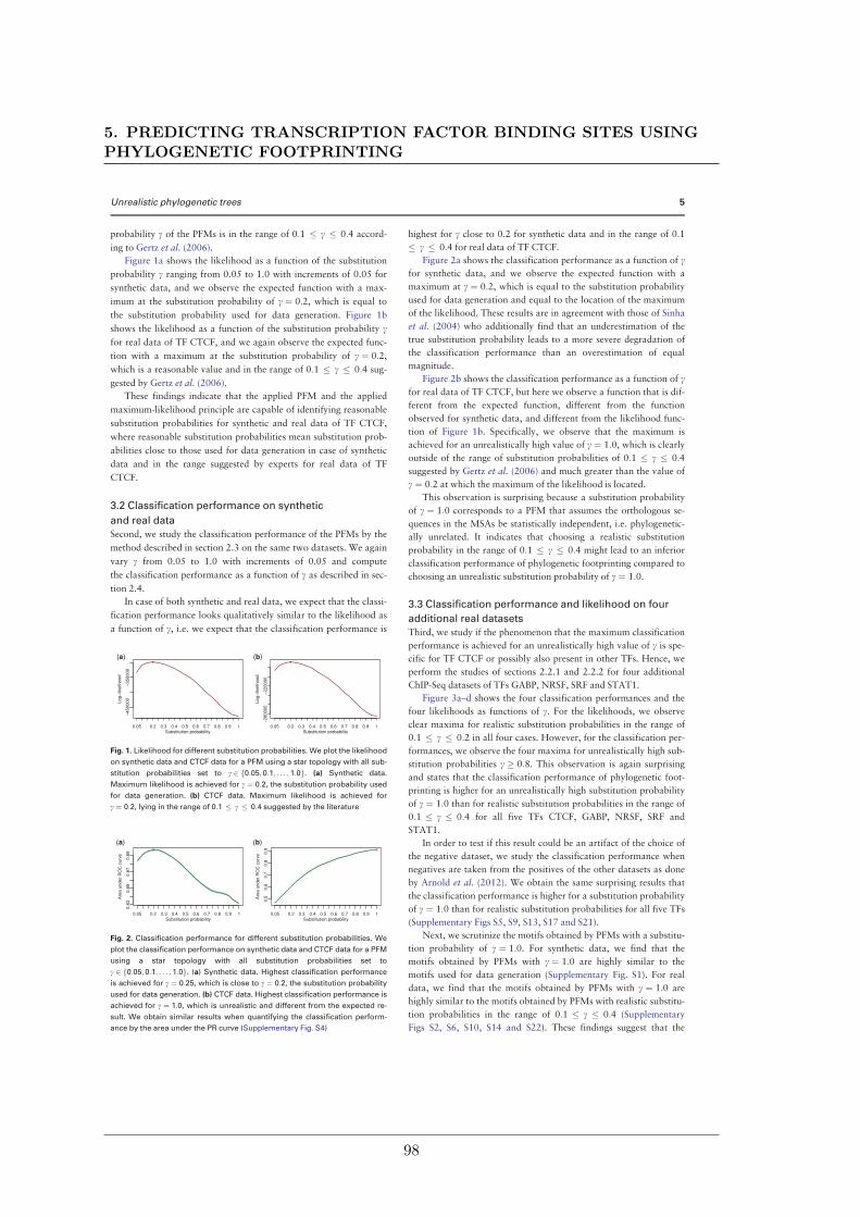
probability c of the PFMs is in the range of 0:1 � c � 0:4 accord-

ing to Gertz et al. (2006).

Figure 1a shows the likelihood as a function of the substitution

probability c ranging from 0.05 to 1.0 with increments of 0.05 for

synthetic data, and we observe the expected function with a max-

imum at the substitution probability of c ¼ 0:2, which is equal to

the substitution probability used for data generation. Figure 1b

shows the likelihood as a function of the substitution probability c

for real data of TF CTCF, and we again observe the expected func-

tion with a maximum at the substitution probability of c ¼ 0:2,

which is a reasonable value and in the range of 0:1 � c � 0:4 sug-

gested by Gertz et al. (2006).

These findings indicate that the applied PFM and the applied

maximum-likelihood principle are capable of identifying reasonable

substitution probabilities for synthetic and real data of TF CTCF,

where reasonable substitution probabilities mean substitution prob-

abilities close to those used for data generation in case of synthetic

data and in the range suggested by experts for real data of TF

CTCF.

3.2 Classification performance on synthetic

and real dataSecond, we study the classification performance of the PFMs by the

method described in section 2.3 on the same two datasets. We again

vary c from 0.05 to 1.0 with increments of 0.05 and compute

the classification performance as a function of c as described in sec-

tion 2.4.

In case of both synthetic and real data, we expect that the classi-

fication performance looks qualitatively similar to the likelihood as

a function of c, i.e. we expect that the classification performance is

highest for c close to 0.2 for synthetic data and in the range of 0:1

� c � 0:4 for real data of TF CTCF.

Figure 2a shows the classification performance as a function of c

for synthetic data, and we observe the expected function with a

maximum at c ¼ 0:2, which is equal to the substitution probability

used for data generation and equal to the location of the maximum

of the likelihood. These results are in agreement with those of Sinha

et al. (2004) who additionally find that an underestimation of the

true substitution probability leads to a more severe degradation of

the classification performance than an overestimation of equal

magnitude.

Figure 2b shows the classification performance as a function of c

for real data of TF CTCF, but here we observe a function that is dif-

ferent from the expected function, different from the function

observed for synthetic data, and different from the likelihood func-

tion of Figure 1b. Specifically, we observe that the maximum is

achieved for an unrealistically high value of c ¼ 1:0, which is clearly

outside of the range of substitution probabilities of 0:1 � c � 0:4

suggested by Gertz et al. (2006) and much greater than the value of

c ¼ 0:2 at which the maximum of the likelihood is located.

This observation is surprising because a substitution probability

of c ¼ 1:0 corresponds to a PFM that assumes the orthologous se-

quences in the MSAs be statistically independent, i.e. phylogenetic-

ally unrelated. It indicates that choosing a realistic substitution

probability in the range of 0:1 � c � 0:4 might lead to an inferior

classification performance of phylogenetic footprinting compared to

choosing an unrealistic substitution probability of c ¼ 1:0.

3.3 Classification performance and likelihood on four

additional real datasetsThird, we study if the phenomenon that the maximum classification

performance is achieved for an unrealistically high value of c is spe-

cific for TF CTCF or possibly also present in other TFs. Hence, we

perform the studies of sections 2.2.1 and 2.2.2 for four additional

ChIP-Seq datasets of TFs GABP, NRSF, SRF and STAT1.

Figure 3a–d shows the four classification performances and the

four likelihoods as functions of c. For the likelihoods, we observe

clear maxima for realistic substitution probabilities in the range of

0:1 � c � 0:2 in all four cases. However, for the classification per-

formances, we observe the four maxima for unrealistically high sub-

stitution probabilities c � 0:8. This observation is again surprising

and states that the classification performance of phylogenetic foot-

printing is higher for an unrealistically high substitution probability

of c ¼ 1:0 than for realistic substitution probabilities in the range of

0:1 � c � 0:4 for all five TFs CTCF, GABP, NRSF, SRF and

STAT1.

In order to test if this result could be an artifact of the choice of

the negative dataset, we study the classification performance when

negatives are taken from the positives of the other datasets as done

by Arnold et al. (2012). We obtain the same surprising results that

the classification performance is higher for a substitution probability

of c ¼ 1:0 than for realistic substitution probabilities for all five TFs

(Supplementary Figs S5, S9, S13, S17 and S21).

Next, we scrutinize the motifs obtained by PFMs with a substitu-

tion probability of c ¼ 1:0. For synthetic data, we find that the

motifs obtained by PFMs with c ¼ 1:0 are highly similar to the

motifs used for data generation (Supplementary Fig. S1). For real

data, we find that the motifs obtained by PFMs with c ¼ 1:0 are

highly similar to the motifs obtained by PFMs with realistic substitu-

tion probabilities in the range of 0:1 � c � 0:4 (Supplementary

Figs S2, S6, S10, S14 and S22). These findings suggest that the

(a) (b)

Fig. 1. Likelihood for different substitution probabilities. We plot the likelihood

on synthetic data and CTCF data for a PFM using a star topology with all sub-

stitution probabilities set to c 2 f0:05; 0:1; . . . ; 1:0g. (a) Synthetic data.

Maximum likelihood is achieved for c ¼ 0:2, the substitution probability used

for data generation. (b) CTCF data. Maximum likelihood is achieved for

c ¼ 0:2, lying in the range of 0:1 � c � 0:4 suggested by the literature

(a) (b)

Fig. 2. Classification performance for different substitution probabilities. We

plot the classification performance on synthetic data and CTCF data for a PFM

using a star topology with all substitution probabilities set to

c 2 f0:05; 0:1; . . . ; 1:0g. (a) Synthetic data. Highest classification performance

is achieved for c ¼ 0:25, which is close to c ¼ 0:2, the substitution probability

used for data generation. (b) CTCF data. Highest classification performance is

achieved for c ¼ 1:0, which is unrealistic and different from the expected re-

sult. We obtain similar results when quantifying the classification perform-

ance by the area under the PR curve (Supplementary Fig. S4)

Unrealistic phylogenetic trees 5

5. PREDICTING TRANSCRIPTION FACTOR BINDING SITES USINGPHYLOGENETIC FOOTPRINTING

98

Page 109

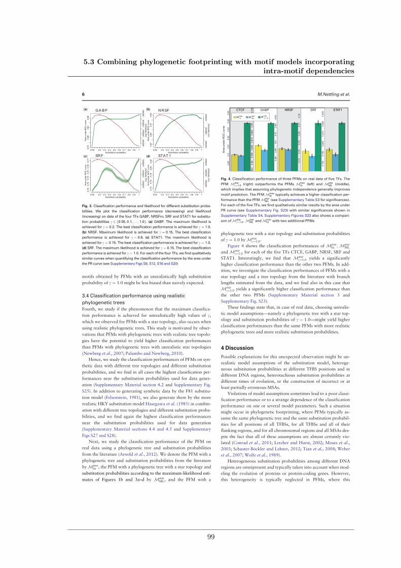
motifs obtained by PFMs with an unrealistically high substitution

probability of c ¼ 1:0 might be less biased than naively expected.

3.4 Classification performance using realistic

phylogenetic treesFourth, we study if the phenomenon that the maximum classifica-

tion performance is achieved for unrealistically high values of c,

which we observed for PFMs with a star topology, also occurs when

using realistic phylogenetic trees. This study is motivated by obser-

vations that PFMs with phylogenetic trees with realistic tree topolo-

gies have the potential to yield higher classification performances

than PFMs with phylogenetic trees with unrealistic star topologies

(Newberg et al., 2007; Palumbo and Newberg, 2010).

Hence, we study the classification performances of PFMs on syn-

thetic data with different tree topologies and different substitution

probabilities, and we find in all cases the highest classification per-

formances near the substitution probabilities used for data gener-

ation (Supplementary Material section 4.2 and Supplementary Fig.

S25). In addition to generating synthetic data by the F81 substitu-

tion model (Felsenstein, 1981), we also generate them by the more

realistic HKY substitution model Hasegawa et al. (1985) in combin-

ation with different tree topologies and different substitution proba-

bilities, and we find again the highest classification performances

near the substitution probabilities used for data generation

(Supplementary Material sections 4.4 and 4.5 and Supplementary

Figs S27 and S28).

Next, we study the classification performance of the PFM on

real data using a phylogenetic tree and substitution probabilities

from the literature (Arnold et al., 2012). We denote the PFM with a

phylogenetic tree and substitution probabilities from the literature

byMtreelit , the PFM with a phylogenetic tree with a star topology and

substitution probabilities according to the maximum-likelihood esti-

mates of Figures 1b and 3a–d by MstarML, and the PFM with a

phylogenetic tree with a star topology and substitution probabilities

of c ¼ 1:0 byMstarc¼1:0.

Figure 4 shows the classification performances of Mtreelit ;Mstar

ML

andMstarc¼1:0 for each of the five TFs CTCF, GABP, NRSF, SRF and

STAT1. Interestingly, we find that Mstarc¼1:0 yields a significantly

higher classification performance than the other two PFMs. In add-

ition, we investigate the classification performances of PFMs with a

star topology and a tree topology from the literature with branch

lengths estimated from the data, and we find also in this case that

Mstarc¼1:0 yields a significantly higher classification performance than

the other two PFMs (Supplementary Material section 3 and

Supplementary Fig. S23).

These findings state that, in case of real data, choosing unrealis-

tic model assumptions—namely a phylogenetic tree with a star top-

ology and substitution probabilities of c ¼ 1:0—might yield higher

classification performances than the same PFMs with more realistic

phylogenetic trees and more realistic substitution probabilities.

4 Discussion

Possible explanations for this unexpected observation might be un-

realistic model assumptions of the substitution model, heteroge-

neous substitution probabilities at different TFBS positions and in

different DNA regions, heterotachious substitution probabilities at

different times of evolution, or the construction of incorrect or at

least partially erroneous MSAs.

Violations of model assumptions sometimes lead to a poor classi-

fication performance or to a strange dependence of the classification

performance on one or several model parameters. Such a situation

might occur in phylogenetic footprinting, where PFMs typically as-

sume the same phylogenetic tree and the same substitution probabil-

ities for all positions of all TFBSs, for all TFBSs and all of their

flanking regions, and for all chromosomal regions and all MSAs des-

pite the fact that all of these assumptions are almost certainly vio-

lated (Conrad et al., 2011; Lercher and Hurst, 2002; Moses et al.,

2003; Schuster-Bockler and Lehner, 2012; Tian et al., 2008; Weber

et al., 2007; Wolfe et al., 1989).

Heterogeneous substitution probabilities among different DNA

regions are omnipresent and typically taken into account when mod-

eling the evolution of proteins or protein-coding genes. However,

this heterogeneity is typically neglected in PFMs, where this

Fig. 4. Classification performance of three PFMs on real data of five TFs. The

PFM Mstarc¼1:0 (right) outperforms the PFMs Mtree

lit (left) and MstarML (middle),

which implies that assuming phylogenetic independence generally improves

motif prediction. The PFMMtreelit typically achieves a higher classification per-

formance than the PFMMstarML (see Supplementary Table S3 for significances).

For each of the five TFs, we find qualitatively similar results by the area under

PR curve (see Supplementary Fig. S23) with similar significances shown in

Supplementary Table S4. Supplementary Figures S23 also shows a compari-

son ofMstarc¼1:0;Mstar

ML andMtreelit with two additional PFMs

(a) (b)

(c) (d)

Fig. 3. Classification performance and likelihood for different substitution proba-

bilities. We plot the classification performance (decreasing) and likelihood

(increasing) on data of the four TFs GABP, NRSFm, SRF and STAT1 for substitu-

tion probabilities c 2 f0:05; 0:1; . . . ; 1:0g. (a) GABP. The maximum likelihood is

achieved for c ¼ 0:2. The best classification performance is achieved for c ¼ 1:0.

(b) NRSF. Maximum likelihood is achieved for c ¼ 0:15. The best classification

performance is achieved for c ¼ 0:8. (c) STAT1. The maximum likelihood is

achieved for c ¼ 0:15. The best classification performance is achieved for c ¼ 1:0.

(d) SRF. The maximum likelihood is achieved for c ¼ 0:15. The best classification

performance is achieved for c ¼ 1:0. For each of the four TFs, we find qualitatively

similar curves when quantifying the classification performance by the area under

the PR curve (see Supplementary Figs S8, S12, S16 and S20)

6 M.Nettling et al.

5.3 Combining phylogenetic footprinting with motif models incorporatingintra-motif dependencies

99

Page 110

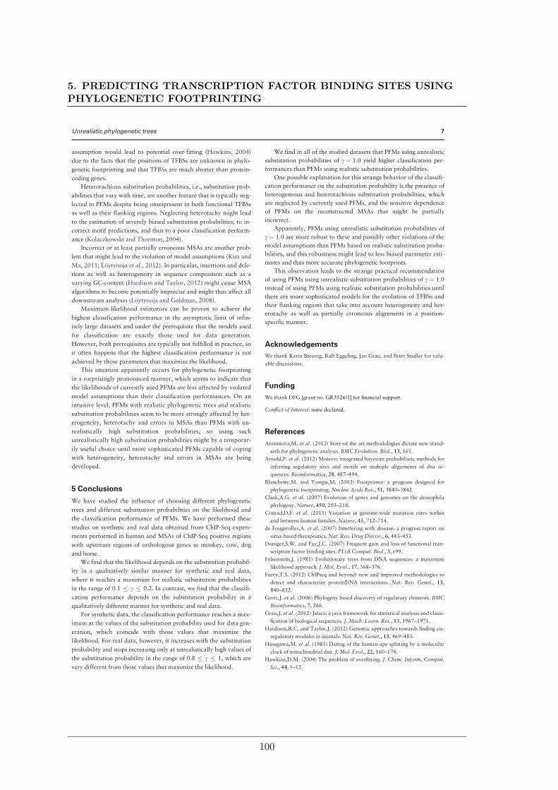
assumption would lead to potential over-fitting (Hawkins, 2004)

due to the facts that the positions of TFBSs are unknown in phylo-

genetic footprinting and that TFBSs are much shorter than protein-

coding genes.

Heterotachious substitution probabilities, i.e., substitution prob-

abilities that vary with time, are another feature that is typically neg-

lected in PFMs despite being omnipresent in both functional TFBSs

as well as their flanking regions. Neglecting heterotachy might lead

to the estimation of severely biased substitution probabilities, to in-

correct motif predictions, and thus to a poor classification perform-

ance (Kolaczkowski and Thornton, 2004).

Incorrect or at least partially erroneous MSAs are another prob-

lem that might lead to the violation of model assumptions (Kim and

Ma, 2011; Loytynoja et al., 2012). In particular, insertions and dele-

tions as well as heterogeneity in sequence composition such as a

varying GC-content (Hardison and Taylor, 2012) might cause MSA

algorithms to become potentially imprecise and might thus affect all

downstream analyses (Loytynoja and Goldman, 2008).

Maximum-likelihood estimators can be proven to achieve the

highest classification performance in the asymptotic limit of infin-

itely large datasets and under the prerequisite that the models used

for classification are exactly those used for data generation.

However, both prerequisites are typically not fulfilled in practice, so

it often happens that the highest classification performance is not

achieved by those parameters that maximize the likelihood.

This situation apparently occurs for phylogenetic footprinting

in a surprisingly pronounced manner, which seems to indicate that

the likelihoods of currently used PFMs are less affected by violated

model assumptions than their classification performances. On an

intuitive level, PFMs with realistic phylogenetic trees and realistic

substitution probabilities seem to be more strongly affected by het-

erogeneity, heterotachy and errors in MSAs than PFMs with un-

realistically high substitution probabilities, so using such

unrealistically high substitution probabilities might by a temporar-

ily useful choice until more sophisticated PFMs capable of coping

with heterogeneity, heterotachy and errors in MSAs are being

developed.

5 Conclusions

We have studied the influence of choosing different phylogenetic

trees and different substitution probabilities on the likelihood and

the classification performance of PFMs. We have performed these

studies on synthetic and real data obtained from ChIP-Seq experi-

ments performed in human and MSAs of ChIP-Seq positive regions

with upstream regions of orthologous genes in monkey, cow, dog

and horse.

We find that the likelihood depends on the substitution probabil-

ity in a qualitatively similar manner for synthetic and real data,

where it reaches a maximum for realistic substitution probabilities

in the range of 0:1 � c � 0:2. In contrast, we find that the classifi-

cation performance depends on the substitution probability in a

qualitatively different manner for synthetic and real data.

For synthetic data, the classification performance reaches a max-

imum at the values of the substitution probability used for data gen-

eration, which coincide with those values that maximize the

likelihood. For real data, however, it increases with the substitution

probability and stops increasing only at unrealistically high values of

the substitution probability in the range of 0:8 � c � 1, which are

very different from those values that maximize the likelihood.

We find in all of the studied datasets that PFMs using unrealistic

substitution probabilities of c ¼ 1:0 yield higher classification per-

formances than PFMs using realistic substitution probabilities.

One possible explanation for this strange behavior of the classifi-

cation performance on the substitution probability is the presence of

heterogeneous and heterotachious substitution probabilities, which

are neglected by currently used PFMs, and the sensitive dependence

of PFMs on the reconstructed MSAs that might be partially

incorrect.

Apparently, PFMs using unrealistic substitution probabilities of

c ¼ 1:0 are more robust to these and possibly other violations of the

model assumptions than PFMs based on realistic substitution proba-

bilities, and this robustness might lead to less biased parameter esti-

mates and thus more accurate phylogenetic footprints.

This observation leads to the strange practical recommendation

of using PFMs using unrealistic substitution probabilities of c ¼ 1:0

instead of using PFMs using realistic substitution probabilities until

there are more sophisticated models for the evolution of TFBSs and

their flanking regions that take into account heterogeneity and het-

erotachy as well as partially erroneous alignments in a position-

specific manner.

Acknowledgements

We thank Karin Breunig, Ralf Eggeling, Jan Grau, and Peter Stadler for valu-

able discussions.

Funding

We thank DFG [grant no. GR3526/1] for financial support.

Conflict of Interest: none declared.

References

Anisimova,M. et al. (2013) State-of the art methodologies dictate new stand-

ards for phylogenetic analysis. BMC Evolution. Biol., 13, 161.

Arnold,P. et al. (2012) Motevo: integrated bayesian probabilistic methods for

inferring regulatory sites and motifs on multiple alignments of dna se-

quences. Bioinformatics, 28, 487–494.

Blanchette,M. and Tompa,M. (2003) Footprinter: a program designed for

phylogenetic footprinting. Nucleic Acids Res., 31, 3840–3842.

Clark,A.G. et al. (2007) Evolution of genes and genomes on the drosophila

phylogeny. Nature, 450, 203–218.

Conrad,D.F. et al. (2011) Variation in genome-wide mutation rates within

and between human families. Nature, 43, 712–714.

de Fougerolles,A. et al. (2007) Interfering with disease: a progress report on

sirna-based therapeutics. Nat. Rev. Drug Discov., 6, 443–453.

Doniger,S.W. and Fay,J.C. (2007) Frequent gain and loss of functional tran-

scription factor binding sites. PLoS Comput. Biol., 3, e99.

Felsenstein,J. (1981) Evolutionary trees from DNA sequences: a maximum

likelihood approach. J. Mol. Evol., 17, 368–376.

Furey,T.S. (2012) ChIPseq and beyond: new and improved methodologies to

detect and characterize proteinDNA interactions. Nat. Rev. Genet., 13,

840–852.

Gertz,J. et al. (2006) Phylogeny based discovery of regulatory elements. BMC

Bioinformatics, 7, 266.

Grau,J. et al. (2012) Jstacs: a java framework for statistical analysis and classi-

fication of biological sequences. J. Mach. Learn. Res., 13, 1967–1971.

Hardison,R.C. and Taylor,J. (2012) Genomic approaches towards finding cis-

regulatory modules in animals. Nat. Rev. Genet., 13, 469–483.

Hasegawa,M. et al. (1985) Dating of the human-ape splitting by a molecular

clock of mitochondrial dna. J. Mol. Evol., 22, 160–174.

Hawkins,D.M. (2004) The problem of overfitting. J. Chem. Inform. Comput.

Sci., 44, 1–12.

Unrealistic phylogenetic trees 7

5. PREDICTING TRANSCRIPTION FACTOR BINDING SITES USINGPHYLOGENETIC FOOTPRINTING

100

Page 111

Hawkins,J. et al. (2009) Assessing phylogenetic motif models for predicting

transcription factor binding sites. Bioinformatics, 25, i339–i347.

Hobert,O. (2008) Gene regulation by transcription factors and micrornas.

Science, 319, 1785–1786.

Jothi,R. et al. (2008) Genome-wide identification of in vivo protein-dna bind-

ing sites from chip-seq data. Nucl. Acids Res., 36, 5221–5231.

Jukes,T.H. and Cantor,C.R. (1969) Evolution of protein molecules. Mammal.

Protein Metab., 3, 132.

Katoh,K. and Standley,D.M. (2013) Mafft multiple sequence alignment soft-

ware version 7: improvements in performance and usability. Mol. Biol.

Evol., 30, 772–780.

Kc,D.B. and Livesay,D.R. (2011) Topology improves phylogenetic motif func-

tional site predictions. IEEE/ACM Transactions on Computational Biology

and Bioinformatics (TCBB), vol. 8, 226–233.

Kim,J. and Ma,J. (2011) Psar: measuring multiple sequence alignment reliabil-

ity by probabilistic sampling. Nucleic Acids Res., 39, 6359–6368.

Kolaczkowski,B. and Thornton,J.W. (2004) Performance of maximum parsi-

mony and likelihood phylogenetics when evolution is heterogeneous.

Nature, 431, 980–984.

Kulakovskiy,I.V. et al. (2010) Deep and wide digging for binding motifs in

chip-seq data. Bioinformatics, 26, 2622–2623.

Lasken,R.S. and McLean,J.S. (2014) Recent advances in genomic DNA

sequencing of microbial species from single cells. Nat. Rev. Genet., 15,

577–584.

Lawrence,C.E. and Reilly,A.A. (1990) An expectation maximization (em) al-

gorithm for the identification and characterization of common sites in un-

aligned biopolymer sequences. Proteins, 7, 41–51.

Lercher,M.J. and Hurst,L.D. (2002) Human snp variability and mutation rate

are higher in regions of high recombination. Trends Genet., 18, 337–340.

Loytynoja,A. and Goldman,N. (2008) Phylogeny-aware gap placement pre-

vents errors in sequence alignment and evolutionary analysis. Science, 320,

1632–1635.

Loytynoja,A. and Goldman,N. (2010) webprank: a phylogeny-aware multiple

sequence aligner with interactive alignment browser. BMC Bioinformatics,

11, 579.

Loytynoja,A. et al. (2012) Accurate extension of multiple sequence alignments

using a phylogeny-aware graph algorithm. Bioinformatics, 28, 1684–1691.

Luco,R.F. et al. (2010) Regulation of alternative splicing by histone modifica-

tions. Science, 327, 996–1000.

Moses,A.M. et al. (2004a) Monkey: identifying conserved transcription-factor

binding sites in multiple alignments using a binding site-specific evolution-

ary model. Genome Biol., 5, R98.

Moses,A.M. et al. (2003) Position specific variation in the rate of evolution in

transcription factor binding sites. BMC Evol. Biol., 3, 19.

Moses,A.M. et al. (2004) Phylogenetic motif detection by expectation-

maximization on evolutionary mixtures. Pacific Symposium on

Biocomputing. Hawaii, United States, pp. 324–335.

Nettling,M. et al. (2017) Combining phylogenetic footprinting with motif mod-

els incorporating intra-motif dependencies. BMC Bioinformatics (In press).

Newberg,L.A. et al. (2007) A phylogenetic gibbs sampler that yields centroid

solutions for cis-regulatory site prediction. Bioinformatics, 23, 1718–1727.

Notredame,C. et al. (2000) T-coffee: A novel method for fast and accurate

multiple sequence alignment. J. Mol. Biol., 302, 205–217.

Nowrousian,M. (2010) Next-generation sequencing techniques for eukaryotic

microorganisms: sequencing-based solutions to biological problems.

Eukaryot. Cell, 9, 1300–1310.

Palumbo,M.J. and Newberg,L.A. (2010) Phyloscan: locating transcription-

regulating binding sites in mixed aligned and unaligned sequence data.

Nucleic Acids Res., 38, W268–W274.

Pollard,K.S. et al. (2010) Detection of nonneutral substitution rates on mam-

malian phylogenies. Genome Res., 20, 110–121.

Sainsbury,S. et al. (2015) Structural basis of transcription initiation by RNA

polymerase II. Nat. Rev. Mol. Cell Biol., 16, 129–143.

Schaefke,B. et al. (2015) Gains and losses of transcription factor binding sites

in saccharomyces cerevisiae and saccharomyces paradoxus. Genome Biol.

Evol., 7, 2245–2257.

Schoenberg,D.R. and Maquat,L.E. (2012) Regulation of cytoplasmic mRNA

decay. Nat. Rev.. Genet., 13, 246–259.

Schuster-Bockler,B. and Lehner,B. (2012) Chromatin organization is a major

influence on regional mutation rates in human cancer cells. Nature, 488,

504–507.

Siddharthan,R. (2008) Phylogibbs-mp: module prediction and discriminative

motif-finding by gibbs sampling. PLoS Comput. Biol., 4, e1000156.

Siddharthan,R. et al. (2005) PhyloGibbs: a gibbs sampling motif finder that in-

corporates phylogeny. PLoS Comput. Biol., 1, e67.

Sinha,S. et al. (2004) PhyME: a probabilistic algorithm for finding motifs in

sets of orthologous sequences. BMC Bioinformatics, 5, 170.

Smith,Z.D. and Meissner,A. (2013) DNA methylation: roles in mammalian

development. Nat. Rev. Genet., 14, 204–220.

Sultan,M. et al. (2008) A global view of gene activity and alternative splicing

by deep sequencing of the human transcriptome. Science, 321, 956–960.

Tam,O.H. et al. (2008) Pseudogene-derived small interfering rnas regulate

gene expression in mouse oocytes. Nature, 453, 534–538.

Tessarz,P. and Kouzarides,T. (2014) Histone core modifications regulating nu-

cleosome structure and dynamics. Nat. Rev. Mol. Cell Biol., 15, 703–708.

Tian,D. et al. (2008) Single-nucleotide mutation rate increases close to inser-

tions/deletions in eukaryotes. Nature, 455, 105–108.

Tu�grul,M. et al. (2015) Dynamics of transcription factor binding site evolu-

tion. PLoS Genet., 11, e1005639.

Valouev,A. et al. (2008) Genome-wide analysis of transcription factor binding

sites based on chip-seq data. Nat. Methods, 5, 829–834.

van Dijk,E.L. et al. (2016) Ten years of next-generation sequencing technol-

ogy. Trends Genet., 30, 418–426.

Villar,D. et al. (2014) Evolution of transcription factor binding in metazoans -

mechanisms and functional implications. Nat. Rev. Genet., 15, 221–233.

Voss,T.C. and Hager,G.L. (2014) Dynamic regulation of transcriptional states

by chromatin and transcription factors. Nat. Rev. Genet., 15, 69–81.

Weber,M. et al. (2007) Distribution, silencing potential and evolutionary im-

pact of promoter dna methylation in the human genome. Nat. Genet., 39,

457–466.

Wolfe,K.H. et al. (1989) Mutation rates differ among regions of the mamma-

lian genome. Nature, 283–285. pages

8 M.Nettling et al.

5.3 Combining phylogenetic footprinting with motif models incorporatingintra-motif dependencies

101

Page 112

5. PREDICTING TRANSCRIPTION FACTOR BINDING SITES USINGPHYLOGENETIC FOOTPRINTING

102

Page 113

6 Visualisation of motifs

6.1 DiffLogo: A comparative visualisation of sequence motifs

M Nettling*, H Treutler*, J Grau, J Keilwagen, S Posch, I Grosse. 2015. DiffLogo: acomparative visualization of sequence motifs. BMC bioinformatics, 16:1 doi:10.1186/s12859-015-0767-x

103

Page 114

Nettling et al. BMC Bioinformatics (2015) 16:387 DOI 10.1186/s12859-015-0767-x

SOFTWARE Open Access

DiffLogo: a comparative visualization ofsequence motifsMartin Nettling1*†, Hendrik Treutler2†, Jan Grau1, Jens Keilwagen3, Stefan Posch1 and Ivo Grosse1,4

Abstract

Background: For three decades, sequence logos are the de facto standard for the visualization of sequence motifs inbiology and bioinformatics. Reasons for this success story are their simplicity and clarity. The number of inferred andpublished motifs grows with the number of data sets and motif extraction algorithms. Hence, it becomes more andmore important to perceive differences between motifs. However, motif differences are hard to detect from individualsequence logos in case of multiple motifs for one transcription factor, highly similar binding motifs of differenttranscription factors, or multiple motifs for one protein domain.

Results: Here, we present DiffLogo, a freely available, extensible, and user-friendly R package for visualizing motifdifferences. DiffLogo is capable of showing differences between DNA motifs as well as protein motifs in a pair-wisemanner resulting in publication-ready figures. In case of more than two motifs, DiffLogo is capable of visualizingpair-wise differences in a tabular form. Here, the motifs are ordered by similarity, and the difference logos are coloredfor clarity. We demonstrate the benefit of DiffLogo on CTCF motifs from different human cell lines, on E-box motifs ofthree basic helix-loop-helix transcription factors as examples for comparison of DNA motifs, and on F-box domainsfrom three different families as example for comparison of protein motifs.

Conclusions: DiffLogo provides an intuitive visualization of motif differences. It enables the illustration andinvestigation of differences between highly similar motifs such as binding patterns of transcription factors for differentcell types, treatments, and algorithmic approaches.

Keywords: Sequence analysis, Sequence logo, Sequence motif, Position weight matrix, Binding sites

BackgroundBiological polymer sequences encode information by theorder of their monomers, i.e., bases or amino acids. Oftenspecific parts of the polymer sequence are of particularinterest, as they encode, for instance, the binding of tran-scription factors to specific binding sites [1, 2], the bindingto micro-RNA-targets in mRNAs, splice donor sites andsplice acceptor sites in pre-mRNAs [3, 4], the presenceof phosphorylation sites in proteins, or the folding ofspecific protein domains [5]. The set of subsequences ofone specific biological process are often represented as asequence motif.A sequence motif is a model, that represents the pref-

erence for the monomers based on a set of aligned

*Correspondence: [email protected]†Equal contributors1Institute of Computer Science, Martin Luther University Halle-Wittenberg,Halle (Saale), GermanyFull list of author information is available at the end of the article

biopolymer sequences. Sequence motifs are the result ofpipelines comprising wet-lab experiments and motif pre-diction algorithms, and are frequently used as the basis ofin silico predictions [6]. Thus, sequence motif are criticalfor research of a wide range of problems in biology andbioinformatics.Considering a particular transcription factor, there are

many pipelines that combine wet-lab experiments such asHT-SELEX [7, 8], ChIP-Seq [9] or DNase-Seq footprinting[10] with motif prediction algorithms such as MEME[2, 11], ChIPMunk [12], POSMO [13], or Dimont [14].Wet-lab experiments differ in their experimental setup,e.g., ecotypes, cell types, developmental stage, timepoints, or treatment, and motif prediction algorithmsdiffer in their mathematical theory and implementationdetails.Visualizing the results of motif discovery is nowa-

days accomplished by sequence logos [15], the de facto

© 2015 Nettling et al. Open Access This article is distributed under the terms of the Creative Commons Attribution 4.0International License (http://creativecommons.org/licenses/by/4.0/), which permits unrestricted use, distribution, andreproduction in any medium, provided you give appropriate credit to the original author(s) and the source, provide a link to theCreative Commons license, and indicate if changes were made. The Creative Commons Public Domain Dedication waiver(http://creativecommons.org/publicdomain/zero/1.0/) applies to the data made available in this article, unless otherwise stated.

6. VISUALISATION OF MOTIFS

104

Page 115

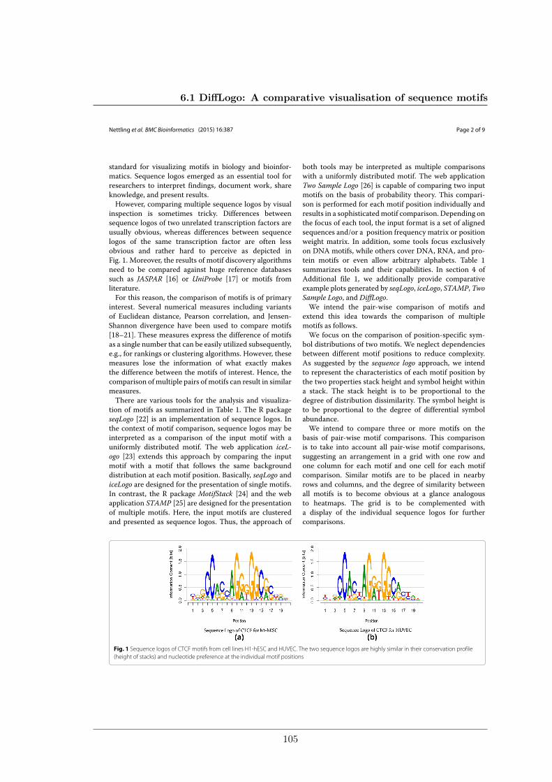
Nettling et al. BMC Bioinformatics (2015) 16:387 Page 2 of 9

standard for visualizing motifs in biology and bioinfor-matics. Sequence logos emerged as an essential tool forresearchers to interpret findings, document work, shareknowledge, and present results.However, comparing multiple sequence logos by visual

inspection is sometimes tricky. Differences betweensequence logos of two unrelated transcription factors areusually obvious, whereas differences between sequencelogos of the same transcription factor are often lessobvious and rather hard to perceive as depicted inFig. 1. Moreover, the results of motif discovery algorithmsneed to be compared against huge reference databasessuch as JASPAR [16] or UniProbe [17] or motifs fromliterature.For this reason, the comparison of motifs is of primary

interest. Several numerical measures including variantsof Euclidean distance, Pearson correlation, and Jensen-Shannon divergence have been used to compare motifs[18–21]. These measures express the difference of motifsas a single number that can be easily utilized subsequently,e.g., for rankings or clustering algorithms. However, thesemeasures lose the information of what exactly makesthe difference between the motifs of interest. Hence, thecomparison ofmultiple pairs of motifs can result in similarmeasures.There are various tools for the analysis and visualiza-

tion of motifs as summarized in Table 1. The R packageseqLogo [22] is an implementation of sequence logos. Inthe context of motif comparison, sequence logos may beinterpreted as a comparison of the input motif with auniformly distributed motif. The web application iceL-ogo [23] extends this approach by comparing the inputmotif with a motif that follows the same backgrounddistribution at each motif position. Basically, seqLogo andiceLogo are designed for the presentation of single motifs.In contrast, the R package MotifStack [24] and the webapplication STAMP [25] are designed for the presentationof multiple motifs. Here, the input motifs are clusteredand presented as sequence logos. Thus, the approach of

both tools may be interpreted as multiple comparisonswith a uniformly distributed motif. The web applicationTwo Sample Logo [26] is capable of comparing two inputmotifs on the basis of probability theory. This compari-son is performed for each motif position individually andresults in a sophisticatedmotif comparison. Depending onthe focus of each tool, the input format is a set of alignedsequences and/or a position frequency matrix or positionweight matrix. In addition, some tools focus exclusivelyon DNA motifs, while others cover DNA, RNA, and pro-tein motifs or even allow arbitrary alphabets. Table 1summarizes tools and their capabilities. In section 4 ofAdditional file 1, we additionally provide comparativeexample plots generated by seqLogo, iceLogo, STAMP, TwoSample Logo, and DiffLogo.We intend the pair-wise comparison of motifs and

extend this idea towards the comparison of multiplemotifs as follows.We focus on the comparison of position-specific sym-

bol distributions of two motifs. We neglect dependenciesbetween different motif positions to reduce complexity.As suggested by the sequence logo approach, we intendto represent the characteristics of each motif position bythe two properties stack height and symbol height withina stack. The stack height is to be proportional to thedegree of distribution dissimilarity. The symbol height isto be proportional to the degree of differential symbolabundance.We intend to compare three or more motifs on the

basis of pair-wise motif comparisons. This comparisonis to take into account all pair-wise motif comparisons,suggesting an arrangement in a grid with one row andone column for each motif and one cell for each motifcomparison. Similar motifs are to be placed in nearbyrows and columns, and the degree of similarity betweenall motifs is to become obvious at a glance analogousto heatmaps. The grid is to be complemented witha display of the individual sequence logos for furthercomparisons.

Fig. 1 Sequence logos of CTCF motifs from cell lines H1-hESC and HUVEC. The two sequence logos are highly similar in their conservation profile(height of stacks) and nucleotide preference at the individual motif positions

6.1 DiffLogo: A comparative visualisation of sequence motifs

105

Page 116

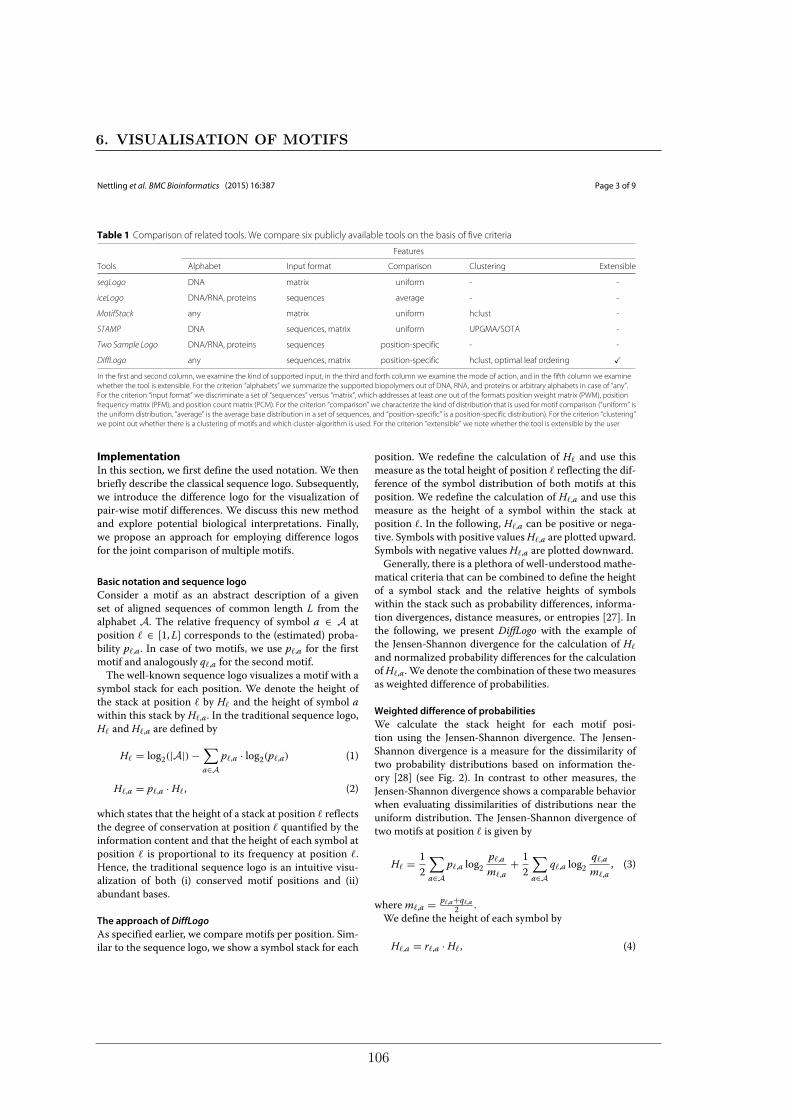
Nettling et al. BMC Bioinformatics (2015) 16:387 Page 3 of 9

Table 1 Comparison of related tools. We compare six publicly available tools on the basis of five criteria

Features

Tools Alphabet Input format Comparison Clustering Extensible

seqLogo DNA matrix uniform - -

iceLogo DNA/RNA, proteins sequences average - -

MotifStack any matrix uniform hclust -

STAMP DNA sequences, matrix uniform UPGMA/SOTA -

Two Sample Logo DNA/RNA, proteins sequences position-specific - -

DiffLogo any sequences, matrix position-specific hclust, optimal leaf ordering �In the first and second column, we examine the kind of supported input, in the third and forth column we examine the mode of action, and in the fifth column we examinewhether the tool is extensible. For the criterion “alphabets” we summarize the supported biopolymers out of DNA, RNA, and proteins or arbitrary alphabets in case of “any”.For the criterion “input format” we discriminate a set of “sequences” versus “matrix”, which addresses at least one out of the formats position weight matrix (PWM), positionfrequency matrix (PFM), and position count matrix (PCM). For the criterion “comparison” we characterize the kind of distribution that is used for motif comparison (“uniform” isthe uniform distribution, “average” is the average base distribution in a set of sequences, and “position-specific” is a position-specific distribution). For the criterion “clustering”we point out whether there is a clustering of motifs and which cluster-algorithm is used. For the criterion “extensible” we note whether the tool is extensible by the user

ImplementationIn this section, we first define the used notation. We thenbriefly describe the classical sequence logo. Subsequently,we introduce the difference logo for the visualization ofpair-wise motif differences. We discuss this new methodand explore potential biological interpretations. Finally,we propose an approach for employing difference logosfor the joint comparison of multiple motifs.

Basic notation and sequence logoConsider a motif as an abstract description of a givenset of aligned sequences of common length L from thealphabet A. The relative frequency of symbol a ∈ A atposition � ∈ [1, L] corresponds to the (estimated) proba-bility p�,a. In case of two motifs, we use p�,a for the firstmotif and analogously q�,a for the second motif.The well-known sequence logo visualizes a motif with a

symbol stack for each position. We denote the height ofthe stack at position � by H� and the height of symbol awithin this stack by H�,a. In the traditional sequence logo,H� and H�,a are defined by

H� = log2(|A|) −∑a∈A

p�,a · log2(p�,a) (1)

H�,a = p�,a · H�, (2)

which states that the height of a stack at position � reflectsthe degree of conservation at position � quantified by theinformation content and that the height of each symbol atposition � is proportional to its frequency at position �.Hence, the traditional sequence logo is an intuitive visu-alization of both (i) conserved motif positions and (ii)abundant bases.

The approach of DiffLogoAs specified earlier, we compare motifs per position. Sim-ilar to the sequence logo, we show a symbol stack for each

position. We redefine the calculation of H� and use thismeasure as the total height of position � reflecting the dif-ference of the symbol distribution of both motifs at thisposition. We redefine the calculation of H�,a and use thismeasure as the height of a symbol within the stack atposition �. In the following, H�,a can be positive or nega-tive. Symbols with positive valuesH�,a are plotted upward.Symbols with negative values H�,a are plotted downward.Generally, there is a plethora of well-understood mathe-

matical criteria that can be combined to define the heightof a symbol stack and the relative heights of symbolswithin the stack such as probability differences, informa-tion divergences, distance measures, or entropies [27]. Inthe following, we present DiffLogo with the example ofthe Jensen-Shannon divergence for the calculation of H�

and normalized probability differences for the calculationofH�,a. We denote the combination of these twomeasuresas weighted difference of probabilities.

Weighted difference of probabilitiesWe calculate the stack height for each motif posi-tion using the Jensen-Shannon divergence. The Jensen-Shannon divergence is a measure for the dissimilarity oftwo probability distributions based on information the-ory [28] (see Fig. 2). In contrast to other measures, theJensen-Shannon divergence shows a comparable behaviorwhen evaluating dissimilarities of distributions near theuniform distribution. The Jensen-Shannon divergence oftwo motifs at position � is given by

H� = 12

∑a∈A

p�,a log2p�,am�,a

+ 12

∑a∈A

q�,a log2q�,am�,a

, (3)

wherem�,a = p�,a+q�,a2 .

We define the height of each symbol by

H�,a = r�,a · H�, (4)

6. VISUALISATION OF MOTIFS

106

Page 117

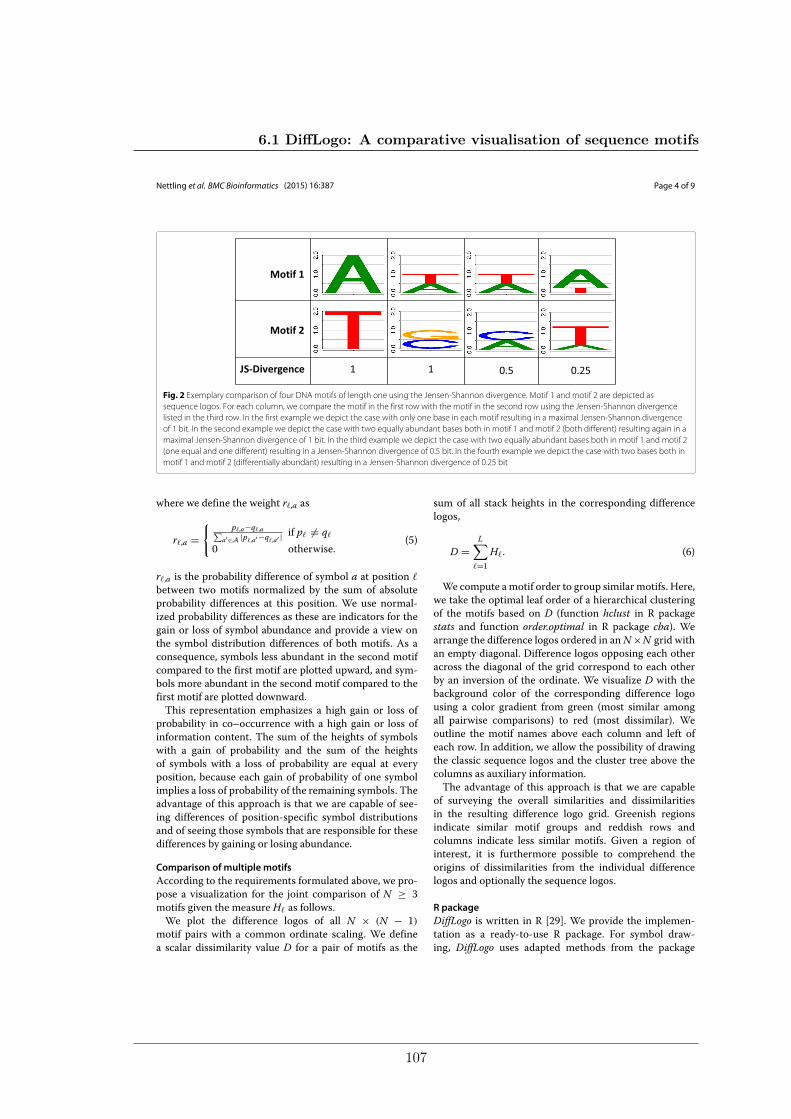
Nettling et al. BMC Bioinformatics (2015) 16:387 Page 4 of 9

Fig. 2 Exemplary comparison of four DNA motifs of length one using the Jensen-Shannon divergence. Motif 1 and motif 2 are depicted assequence logos. For each column, we compare the motif in the first row with the motif in the second row using the Jensen-Shannon divergencelisted in the third row. In the first example we depict the case with only one base in each motif resulting in a maximal Jensen-Shannon divergenceof 1 bit. In the second example we depict the case with two equally abundant bases both in motif 1 and motif 2 (both different) resulting again in amaximal Jensen-Shannon divergence of 1 bit. In the third example we depict the case with two equally abundant bases both in motif 1 and motif 2(one equal and one different) resulting in a Jensen-Shannon divergence of 0.5 bit. In the fourth example we depict the case with two bases both inmotif 1 and motif 2 (differentially abundant) resulting in a Jensen-Shannon divergence of 0.25 bit

where we define the weight r�,a as

r�,a ={ p�,a−q�,a∑

a′∈A |p�,a′−q�,a′ | if p� �= q�

0 otherwise.(5)

r�,a is the probability difference of symbol a at position �

between two motifs normalized by the sum of absoluteprobability differences at this position. We use normal-ized probability differences as these are indicators for thegain or loss of symbol abundance and provide a view onthe symbol distribution differences of both motifs. As aconsequence, symbols less abundant in the second motifcompared to the first motif are plotted upward, and sym-bols more abundant in the second motif compared to thefirst motif are plotted downward.This representation emphasizes a high gain or loss of

probability in co–occurrence with a high gain or loss ofinformation content. The sum of the heights of symbolswith a gain of probability and the sum of the heightsof symbols with a loss of probability are equal at everyposition, because each gain of probability of one symbolimplies a loss of probability of the remaining symbols. Theadvantage of this approach is that we are capable of see-ing differences of position-specific symbol distributionsand of seeing those symbols that are responsible for thesedifferences by gaining or losing abundance.

Comparison of multiple motifsAccording to the requirements formulated above, we pro-pose a visualization for the joint comparison of N ≥ 3motifs given the measure H� as follows.We plot the difference logos of all N × (N − 1)

motif pairs with a common ordinate scaling. We definea scalar dissimilarity value D for a pair of motifs as the

sum of all stack heights in the corresponding differencelogos,

D =L∑

�=1H�. (6)

We compute amotif order to group similar motifs. Here,we take the optimal leaf order of a hierarchical clusteringof the motifs based on D (function hclust in R packagestats and function order.optimal in R package cba). Wearrange the difference logos ordered in anN×N grid withan empty diagonal. Difference logos opposing each otheracross the diagonal of the grid correspond to each otherby an inversion of the ordinate. We visualize D with thebackground color of the corresponding difference logousing a color gradient from green (most similar amongall pairwise comparisons) to red (most dissimilar). Weoutline the motif names above each column and left ofeach row. In addition, we allow the possibility of drawingthe classic sequence logos and the cluster tree above thecolumns as auxiliary information.The advantage of this approach is that we are capable

of surveying the overall similarities and dissimilaritiesin the resulting difference logo grid. Greenish regionsindicate similar motif groups and reddish rows andcolumns indicate less similar motifs. Given a region ofinterest, it is furthermore possible to comprehend theorigins of dissimilarities from the individual differencelogos and optionally the sequence logos.

R packageDiffLogo is written in R [29]. We provide the implemen-tation as a ready-to-use R package. For symbol draw-ing, DiffLogo uses adapted methods from the package

6.1 DiffLogo: A comparative visualisation of sequence motifs

107

Page 118

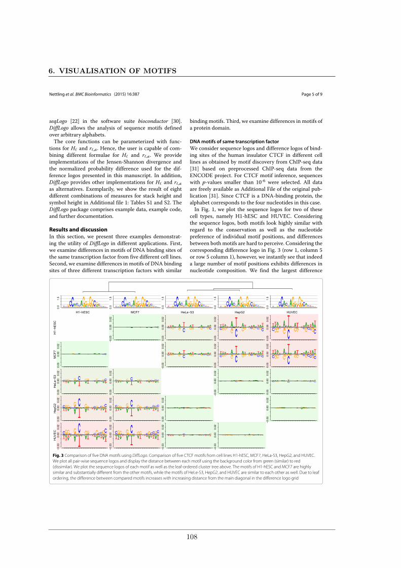
Nettling et al. BMC Bioinformatics (2015) 16:387 Page 5 of 9

seqLogo [22] in the software suite bioconductor [30].DiffLogo allows the analysis of sequence motifs definedover arbitrary alphabets.The core functions can be parameterized with func-

tions for H� and r�,a. Hence, the user is capable of com-bining different formulae for H� and r�,a. We provideimplementations of the Jensen-Shannon divergence andthe normalized probability difference used for the dif-ference logos presented in this manuscript. In addition,DiffLogo provides other implementations for H� and r�,aas alternatives. Exemplarily, we show the result of eightdifferent combinations of measures for stack height andsymbol height in Additional file 1: Tables S1 and S2. TheDiffLogo package comprises example data, example code,and further documentation.

Results and discussionIn this section, we present three examples demonstrat-ing the utility of DiffLogo in different applications. First,we examine differences in motifs of DNA binding sites ofthe same transcription factor from five different cell lines.Second, we examine differences in motifs of DNA bindingsites of three different transcription factors with similar

binding motifs. Third, we examine differences in motifs ofa protein domain.

DNAmotifs of same transcription factorWe consider sequence logos and difference logos of bind-ing sites of the human insulator CTCF in different celllines as obtained by motif discovery from ChIP-seq data[31] based on preprocessed ChIP-seq data from theENCODE project. For CTCF motif inference, sequenceswith p-values smaller than 10-6 were selected. All dataare freely available as Additional File of the original pub-lication [31]. Since CTCF is a DNA-binding protein, thealphabet corresponds to the four nucleotides in this case.In Fig. 1, we plot the sequence logos for two of these

cell types, namely H1-hESC and HUVEC. Consideringthe sequence logos, both motifs look highly similar withregard to the conservation as well as the nucleotidepreference of individual motif positions, and differencesbetween both motifs are hard to perceive. Considering thecorresponding difference logo in Fig. 3 (row 1, column 5or row 5 column 1), however, we instantly see that indeeda large number of motif positions exhibits differences innucleotide composition. We find the largest difference

Fig. 3 Comparison of five DNA motifs using DiffLogo. Comparison of five CTCF motifs from cell lines H1-hESC, MCF7, HeLa-S3, HepG2, and HUVEC.We plot all pair-wise sequence logos and display the distance between each motif using the background color from green (similar) to red(dissimilar). We plot the sequence logos of each motif as well as the leaf-ordered cluster tree above. The motifs of H1-hESC and MCF7 are highlysimilar and substantially different from the other motifs, while the motifs of HeLe-S3, HepG2, and HUVEC are similar to each other as well. Due to leafordering, the difference between compared motifs increases with increasing distance from the main diagonal in the difference logo grid

6. VISUALISATION OF MOTIFS

108

Page 119

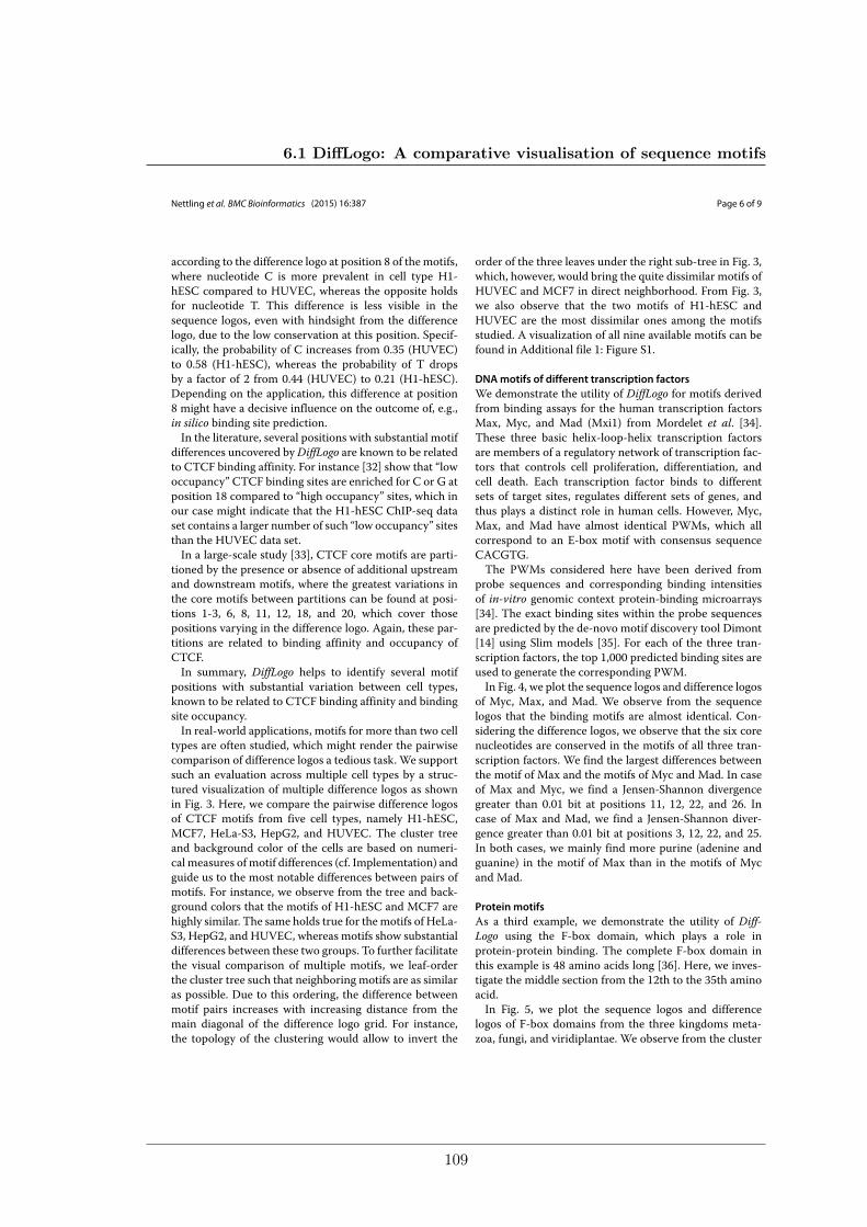
Nettling et al. BMC Bioinformatics (2015) 16:387 Page 6 of 9

according to the difference logo at position 8 of the motifs,where nucleotide C is more prevalent in cell type H1-hESC compared to HUVEC, whereas the opposite holdsfor nucleotide T. This difference is less visible in thesequence logos, even with hindsight from the differencelogo, due to the low conservation at this position. Specif-ically, the probability of C increases from 0.35 (HUVEC)to 0.58 (H1-hESC), whereas the probability of T dropsby a factor of 2 from 0.44 (HUVEC) to 0.21 (H1-hESC).Depending on the application, this difference at position8 might have a decisive influence on the outcome of, e.g.,in silico binding site prediction.In the literature, several positions with substantial motif

differences uncovered byDiffLogo are known to be relatedto CTCF binding affinity. For instance [32] show that “lowoccupancy” CTCF binding sites are enriched for C or G atposition 18 compared to “high occupancy” sites, which inour case might indicate that the H1-hESC ChIP-seq dataset contains a larger number of such “low occupancy” sitesthan the HUVEC data set.In a large-scale study [33], CTCF core motifs are parti-

tioned by the presence or absence of additional upstreamand downstream motifs, where the greatest variations inthe core motifs between partitions can be found at posi-tions 1-3, 6, 8, 11, 12, 18, and 20, which cover thosepositions varying in the difference logo. Again, these par-titions are related to binding affinity and occupancy ofCTCF.In summary, DiffLogo helps to identify several motif

positions with substantial variation between cell types,known to be related to CTCF binding affinity and bindingsite occupancy.In real-world applications, motifs for more than two cell

types are often studied, which might render the pairwisecomparison of difference logos a tedious task. We supportsuch an evaluation across multiple cell types by a struc-tured visualization of multiple difference logos as shownin Fig. 3. Here, we compare the pairwise difference logosof CTCF motifs from five cell types, namely H1-hESC,MCF7, HeLa-S3, HepG2, and HUVEC. The cluster treeand background color of the cells are based on numeri-cal measures of motif differences (cf. Implementation) andguide us to the most notable differences between pairs ofmotifs. For instance, we observe from the tree and back-ground colors that the motifs of H1-hESC and MCF7 arehighly similar. The same holds true for themotifs of HeLa-S3, HepG2, and HUVEC, whereas motifs show substantialdifferences between these two groups. To further facilitatethe visual comparison of multiple motifs, we leaf-orderthe cluster tree such that neighboring motifs are as similaras possible. Due to this ordering, the difference betweenmotif pairs increases with increasing distance from themain diagonal of the difference logo grid. For instance,the topology of the clustering would allow to invert the

order of the three leaves under the right sub-tree in Fig. 3,which, however, would bring the quite dissimilar motifs ofHUVEC and MCF7 in direct neighborhood. From Fig. 3,we also observe that the two motifs of H1-hESC andHUVEC are the most dissimilar ones among the motifsstudied. A visualization of all nine available motifs can befound in Additional file 1: Figure S1.

DNAmotifs of different transcription factorsWe demonstrate the utility of DiffLogo for motifs derivedfrom binding assays for the human transcription factorsMax, Myc, and Mad (Mxi1) from Mordelet et al. [34].These three basic helix-loop-helix transcription factorsare members of a regulatory network of transcription fac-tors that controls cell proliferation, differentiation, andcell death. Each transcription factor binds to differentsets of target sites, regulates different sets of genes, andthus plays a distinct role in human cells. However, Myc,Max, and Mad have almost identical PWMs, which allcorrespond to an E-box motif with consensus sequenceCACGTG.The PWMs considered here have been derived from

probe sequences and corresponding binding intensitiesof in-vitro genomic context protein-binding microarrays[34]. The exact binding sites within the probe sequencesare predicted by the de-novo motif discovery tool Dimont[14] using Slim models [35]. For each of the three tran-scription factors, the top 1,000 predicted binding sites areused to generate the corresponding PWM.In Fig. 4, we plot the sequence logos and difference logos

of Myc, Max, and Mad. We observe from the sequencelogos that the binding motifs are almost identical. Con-sidering the difference logos, we observe that the six corenucleotides are conserved in the motifs of all three tran-scription factors. We find the largest differences betweenthe motif of Max and the motifs of Myc and Mad. In caseof Max and Myc, we find a Jensen-Shannon divergencegreater than 0.01 bit at positions 11, 12, 22, and 26. Incase of Max and Mad, we find a Jensen-Shannon diver-gence greater than 0.01 bit at positions 3, 12, 22, and 25.In both cases, we mainly find more purine (adenine andguanine) in the motif of Max than in the motifs of Mycand Mad.

Protein motifsAs a third example, we demonstrate the utility of Diff-Logo using the F-box domain, which plays a role inprotein-protein binding. The complete F-box domain inthis example is 48 amino acids long [36]. Here, we inves-tigate the middle section from the 12th to the 35th aminoacid.In Fig. 5, we plot the sequence logos and difference

logos of F-box domains from the three kingdoms meta-zoa, fungi, and viridiplantae. We observe from the cluster

6.1 DiffLogo: A comparative visualisation of sequence motifs

109

Page 120

Nettling et al. BMC Bioinformatics (2015) 16:387 Page 7 of 9

Fig. 4 Comparison of E-Box motifs of Max, Myc, and Mad using DiffLogo. We plot all pair-wise difference logos and display the distance betweeneach motif using the background color from green (similar) to red (dissimilar). We plot the sequence logos of each motif as well as the leaf-orderedcluster tree above. The motifs of the transcription factors Myc and Mad are more similar to each other than to the motif Max. The six core nucleotideswith consensus sequence CACGTG are conserved in the motifs of all three transcription factors and, hence, are not visible in the difference logos

tree and the background colors that the motifs of meta-zoa and fungi are highly similar, whereas motifs of thisgroup show substantial differences to viridiplantae. Thelargest difference can be seen between motifs of metazoaand viridiplantae.When comparing metazoa and fungi with viridiplantae,

DiffLogo identifies positions 6, 17, and 22 with high val-ues of the Jensen-Shannon divergence. The differences atpositions 6 and 22 could be expected from the differencesof the sequence logos, whereas the differences at position17 are not immediately obvious from them. At position 6the abundance of arginine (R) in viridiplantae is 0.54 andthus more than 10 times higher than in fungi and 12 timeshigher than inmetazoa. At position 22 tryptophane (W) ishighly abundant in viridiplantae and 4 and 3.4 times moreabundant than in metazoa and fungi. At position 17 themost noticeable differences in viridiplantae to fungi andmetazoa can be seen for amino acid cysteine (C), valine(V), alanine (A), and serine (S). The overall abundanceincreases from 0.13 in metazoa and 0.12 in fungi to 0.64 inviridiplantae. In contrast, the abundance of arginine (R),glutamine (Q), and lysine (K) is only 0.044 in viridiplantaeand 0.44 in metazoa and fungi. A visualization of the

full F-Box domain from four kingdoms can be found inAdditional file 1: Figure S2.

ConclusionWe present DiffLogo, an easy-to-use tool for a fastand efficient comparison of motifs. DiffLogo may beapplied by users with only basic knowledge in R andis highly configurable and extensible for advancedusers. We introduce weighted differences of probabili-ties to emphasize large differences in position-specificsymbol distributions. We present visual comparisonsof multiple motifs stemming from motifs of onetranscription factor in different cell types, differenttranscription factors with similar binding motifs,and species-specific protein domains. Figures gener-ated by DiffLogo enable the identification of overallmotif groups and of sources of dissimilarity. UsingDiffLogo, it is easily possible to compare motifs fromdifferent sources, so DiffLogo facilitates decision making,knowledge sharing, and the presentation of results. Wemake DiffLogo freely available in an extensible, ready-to-use R package including examples and documentation.DiffLogo is part of Bioconductor.

6. VISUALISATION OF MOTIFS

110

Page 121

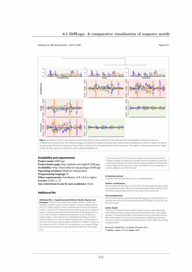
Nettling et al. BMC Bioinformatics (2015) 16:387 Page 8 of 9

Fig. 5 Comparison of three F-box domain motifs using DiffLogo. We compare the F-box domains from the kingdoms metazoa, fungi, andviridiplantae and plot all pair-wise difference logos and display the distance between each motif using the background color from green (similar) tored (dissimilar). We plot the sequence logos of each motif as well as the leaf-ordered cluster tree above. The motifs of metazoa and fungi are highlysimilar. All other pairwise comparisons show substantial differences

Availability and requirementsProject name: DiffLogoProject home page: http://github.com/mgledi/DiffLogoAvailability: http://bioconductor.org/packages/DiffLogoOperating system(s): Platform independentProgramming language: ROther requirements: Installation of R 1.8.0 or higherLicense: LGPL (≥ 2)Any restrictions to use by non-academics: None

Additional file

Additional file 1: Supplementary Methods, Results, Figures, andExamples. This file is structured in four sections. Section 1, Additionalexamples, contains Figures S1 and S2. Figure S1 shows a DiffLogo grid fornine CTCF motifs. Figure S2 shows a DiffLogo grid for four F-box domainmotifs. In section 2, CTCF with and without clustering, we show in detail theimpact of clustering and optimal leaf ordering for a DiffLogo grid of nineCTCF motifs. In section 3, Alternative combinations of stack heights andsymbol weights, we first describe the mathematical background of fourimplementations of H� and two implementations of r�,a . Afterwards, weshow the result of the eight possible combinations in Tables S1 and S2 ontwo sequence motifs. In section 4, Tool comparison, we compare DiffLogowith the five tools seqLogo, iceLogo,MotifStack, STAMP, and Two SampleLogo.

From the set of nine CTCF motifs we selected the pair of motifs with thehighest similarity according to the Jensen-Shannon divergence (GM12878and K562) and the pair of motifs with the lowest similarity according to theJensen-Shannon divergence (H1-hESC and HUVEC) for the comparison ofthe five different tools. (PDF 8775 kb)

Competing interestsThe authors declare that they have no competing interests.

Authors’ contributionsMN conceived the idea. MN, HT, JK, JG, SP, and IG developed the idea and thecomputational methods. MN and HT implemented and tested DiffLogo. All ofthe authors read and approved the final version of the manuscript.

AcknowledgementsWe thank Karin Breunig, Jesus Cerquides, Ralf Eggeling, and Martin Porsch forvaluable discussions and contributing data and DFG (grant no. GR3526/1) forfinancial support.

Author details1Institute of Computer Science, Martin Luther University Halle-Wittenberg,Halle (Saale), Germany. 2Leibniz Institute of Plant Biochemistry, Halle (Saale),Germany. 3Institute for Biosafety in Plant Biotechnology, Julius Kühn-Institut(JKI), Federal Research Centre for Cultivated Plants, Quedlinburg, Germany.4German Centre for Integrative Biodiversity Research (iDiv) Halle-Jena-Leipzig,Leipzig, Germany.

Received: 10 April 2015 Accepted: 8 October 2015

6.1 DiffLogo: A comparative visualisation of sequence motifs

111

Page 122

Nettling et al. BMC Bioinformatics (2015) 16:387 Page 9 of 9

References1. Staden R. Computer methods to locate signals in nucleic acid sequences.

Nucleic Acids Res. 1984;12:505–19.2. Bailey TL, Elkan C. Fitting a mixture model by expectation maximization

to discover motifs in biopolymers. In: Proceedings of the SecondInternational Conference on Intelligent Systems for Molecular Biology.San Diego: Department of Computer Science and Engineering, Universityof California; 1994.

3. Burge C, Karlin S. Prediction of complete gene structures in humangenomic DNA. J Mol Biol. 1997;268(1):78–94.

4. Yeo G, Burge CB. Maximum Entropy Modeling of Short Sequence Motifswith Applications to RNA Splicing Signals. J Comput Biol. 2004;11(2–3):377–94.

5. Sigrist CJ, Cerutti L, de Castro E, Langendijk-Genevaux PS, Bulliard V,Bairoch A, et al. PROSITE, a protein domain database for functionalcharacterization and annotation. Nucleic Acids Res. 2010;38(Databaseissue):161–6. doi:10.1093/nar/gkp885.

6. Elnitski L, Jin VX, Farnham PJ, Jones SJM. Locating mammaliantranscription factor binding sites: A survey of computational andexperimental techniques. Genome Res. 2006;16:4140006.

7. Zhao Y, Granas D, Stormo GD. Inferring binding energies from selectedbinding sites. PLoS Comput Biol. 2009;5(12):1000590.

8. Jolma A, Kivioja T, Toivonen J, Cheng L, Wei G, Enge M, et al.Multiplexed massively parallel selex for characterization of humantranscription factor binding specificities. Genome Res. 2010;20(6):861–73.

9. Johnson DS, Mortazavi A, Myers RM, Wold B. Genome-wide mapping ofin vivo protein-DNA interactions. Science. 2007;316(5830):1497–502.

10. Galas DJ, Schmitz A. DNAse footprinting: a simple method for thedetection of protein-DNA binding specificity. Nucleic Acids Res. 1978;5(9):3157–170. doi:10.1093/nar/5.9.3157.

11. Bailey TL, Williams N, Misleh C, Li WW. Meme: discovering and analyzingdna and protein sequence motifs. Nucleic Acids Res.2006;34(Web-Server-Issue):369–73.

12. Kulakovskiy IV, Boeva VA, Favorov AV, Makeev VJ. Deep and wide diggingfor binding motifs in chip-seq data. Bioinforma. 2010;26(20):2622–23.

13. Ma X, Kulkarni A, Zhang Z, Xuan Z, Serfling R, Zhang MQ. A highlyefficient and effective motif discovery method for chip-seq/chip-chipdata using positional information. Nucleic Acids Res. 2012;40(7):50.

14. Grau J, Posch S, Grosse I, Keilwagen J. A general approach fordiscriminative de novo motif discovery from high-throughput data.Nucleic Acids Res. 2013;41(21):197.

15. Schneider TD, Stephens RM. Sequence logos: a new way to displayconsensus sequences. Nucleic Acids Res. 1990;18(20):6097–100.

16. Sandelin A, Alkema W, Engström P, Wasserman WW, Lenhard B. Jaspar:an open-access database for eukaryotic transcription factor bindingprofiles. Nucleic Acids Res. 2004;32(Database issue):91–4.

17. Newburger DE, Bulyk ML. Uniprobe: an online database of proteinbinding microarray data on protein–dna interactions. Nucleic Acids Res.2009;37(suppl 1):77–82.

18. Hughes JD, Estep PW, Tavazoie S, Church GM. Computationalidentification of cis-regulatory elements associated with groups offunctionally related genes in saccharomyces cerevisiae1. J Mol Biol.2000;296(5):1205–14. doi:10.1006/jmbi.2000.3519.

19. Aerts S, Van Loo P, Thijs G, Moreau Y, De Moor B. Computationaldetection of cis -regulatory modules. Bioinformatics. 2003;19(suppl 2):5–14. doi:10.1093/bioinformatics/btg1052.

20. Harbison CT, Gordon DB, Lee TI, Rinaldi NJ, Macisaac KD, Danford TW,et al. Transcriptional regulatory code of a eukaryotic genome. Nature.2004;431(7004):99–104. doi:10.1038/nature02800.

21. Linhart C, Halperin Y, Shamir R. Transcription factor and microrna motifdiscovery: The amadeus platform and a compendium of metazoan targetsets. Genome Research. 2008;18(7):1180–9. doi:10.1101/gr.076117.108.

22. Bembom O. SeqLogo: Sequence logos for DNA sequence alignments.2015. http://www.bioconductor.org/packages/release/bioc/html/seqLogo.html, accessed 2015.03.05.

23. Colaert N, Helsens K, Martens L, Vandekerckhove J, Gevaert K. Improvedvisualization of protein consensus sequences by iceLogo. Nat Meth.2009;6(11):786–7. doi:10.1038/nmeth1109-786.

24. Jianhong Ou LJZ. MotifStack: Plot Stacked Logos for Single or MultipleDNA, RNA and Amino Acid sequence. http://www.bioconductor.org/packages/release/bioc/html/motifStack.html. Accessed on 13 Feb 2015.

25. Mahony S, Benos PV. STAMP: a web tool for exploring DNA-binding motifsimilarities. Nucleic Acids Res. 2007;35(Web Server issue):272–58.doi:10.1093/nar/gkm272.

26. Vacic V, Iakoucheva LM, Radivojac P. Two sample logo: a graphicalrepresentation of the differences between two sets of sequencealignments. Bioinforma. 2006;22(12):1536–7.doi:10.1093/bioinformatics/btl151.

27. Ali SM, Silvey SD. A general class of coefficients of divergence of onedistribution from another. J R Stat Soc Series B (Methodological).1966;28(1):131–42.

28. Lin J. Divergence measures based on the Shannon entropy. Inf Theory,IEEE Trans on. 1991;37(1):145–51. doi:10.1109/18.61115.

29. R Core Team. R: A Language and Environment for Statistical Computing.Vienna, Austria: R Foundation for Statistical Computing; 2013. http://www.R-project.org/.

30. Gentleman RC, Carey VJ, Bates DM, Bolstad B, Dettling M, Dudoit S,et al. Bioconductor: open software development for computationalbiology and bioinformatics. Genome biology. 2004;5(10):80–16.doi:10.1186/gb-2004-5-10-r80.

31. Eggeling R, Gohr A, Keilwagen J, Mohr M, Posch S, Smith AD, et al. Onthe value of intra-motif dependencies of human insulator protein ctcf.PLoS ONE. 2014;9(1):85629. doi:10.1371/journal.pone.0085629.

32. Plasschaert RN, Vigneau S, Tempera I, Gupta R, Maksimoska J, Everett L,et al. CTCF binding site sequence differences are associated with uniqueregulatory and functional trends during embryonic stem celldifferentiation. Nucleic acids research. 2014;42(2):774–89.doi:10.1093/nar/gkt910.

33. Nakahashi H, Kwon K-RKR, Resch W, Vian L, Dose M, Stavreva D, et al. Agenome-wide map of CTCF multivalency redefines the CTCF code. Cellreports. 2013;3(5):1678–89. doi:10.1016/j.celrep.2013.04.024.

34. Mordelet F, Horton J, Hartemink AJ, Engelhardt BE, Gordân R. Stabilityselection for regression-based models of transcription factor-DNAbinding specificity. Bioinforma. 2013;29(13):117–25.doi:10.1093/bioinformatics/btt221.

35. Keilwagen J, Grau J. Varying levels of complexity in transcription factorbinding motifs. Nucleic Acids Res. 2015;43(18):e119.

36. Finn RD, Bateman A, Clements J, Coggill P, Eberhardt RY, Eddy SR, et al.Pfam: the protein families database. Nucleic Acids Res. 2014;42(D1):222–30. doi:10.1093/nar/gkt1223.

Submit your next manuscript to BioMed Centraland take full advantage of:

• Convenient online submission

• Thorough peer review

• No space constraints or color figure charges

• Immediate publication on acceptance

• Inclusion in PubMed, CAS, Scopus and Google Scholar

• Research which is freely available for redistribution

Submit your manuscript at www.biomedcentral.com/submit

6. VISUALISATION OF MOTIFS

112

Page 123

7 AppendixThe following sections contain important additional studies important for the understand-ing of this thesis. More supplementary studies, figures, and tables can be found in theadditional files of the corresponding articles.

7.1 Detecting and correcting the binding-affinity bias in ChIP-Seq data using inter-species information

The supplementary material of “Detecting and correcting the binding-affinity bias in ChIP-seq data using inter-species information” consists of two additional files. Additional File 1consists of 3 sections. In Section 1, Modeling the binding-affinity bias, we describe how todetermine the likelihood of non-motif-bearing and motif-bearing alignments modeling thecontamination bias and the binding-affinity bias. In Section 2, Example interpretation ofdifference logos, we give an exemplary interpretation of some difference logos. Section 3,Supplementary Figures, contains Supplementary Figures S1-S18. Additional File 2contains the sequence data used in the studies of this work. Here, I provide a copy ofSection 1 of Additional File 1. This section is the mathematical counter part to thesection “Modeling the binding-affinity bias” in “Methods” in the main manuscript, wheremodeling the binding-affinity bias is explained from the data generating perspective.

7.1.1 Modeling the binding-affinity bias

In this section we describe the probabilistic model for modeling the binding-affinity bias.We define the model in mathematical terms by providing the likelihood function. We usethe notation from the manuscript.

Following the data-generating process described in the manuscript, the probability thatthe model generates an alignment Xn can be written as

p(Xn|θ) = p(Xn|Mn = 0, θ) · p(Mn = 0, θ) + p(Xn|Mn = 1, θ) · p(Mn = 1, θ)

= p(Xn|Mn = 0, θ) · α+ p(Xn|Mn = 1, θ) · (1− α)

To complete the model, we need to specify the probability for non-motif-bearing alignmentsp(Xn|Mn = 0, θ) and that for motif-bearing alignments p(Xn|Mn = 1, θ).

113

Page 124

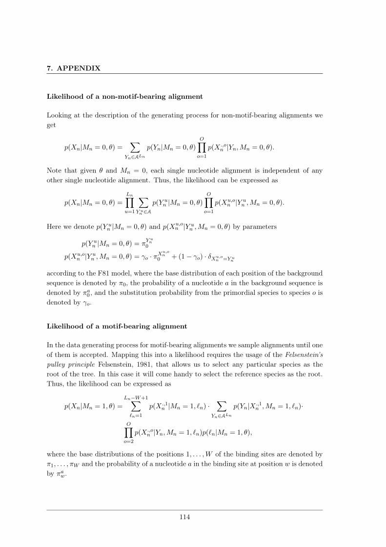
7. APPENDIX

Likelihood of a non-motif-bearing alignment

Looking at the description of the generating process for non-motif-bearing alignments weget

p(Xn|Mn = 0, θ) =∑

Yn∈ALnp(Yn|Mn = 0, θ)

O∏o=1

p(X .,on |Yn,Mn = 0, θ).

Note that given θ and Mn = 0, each single nucleotide alignment is independent of anyother single nucleotide alignment. Thus, the likelihood can be expressed as

p(Xn|Mn = 0, θ) =

Ln∏u=1

∑Y un ∈A

p(Y un |Mn = 0, θ)

O∏o=1

p(Xu,on |Y u

n ,Mn = 0, θ).

Here we denote p(Y un |Mn = 0, θ) and p(Xu,o

n |Y un ,Mn = 0, θ) by parameters

p(Y un |Mn = 0, θ) = π

Y un0

p(Xu,on |Y u

n ,Mn = 0, θ) = γo · πXu,on

0 + (1− γo) · δXu,on =Y un

according to the F81 model, where the base distribution of each position of the backgroundsequence is denoted by π0, the probability of a nucleotide a in the background sequence isdenoted by πa0 , and the substitution probability from the primordial species to species o isdenoted by γo.

Likelihood of a motif-bearing alignment

In the data generating process for motif-bearing alignments we sample alignments until oneof them is accepted. Mapping this into a likelihood requires the usage of the Felsenstein’spulley principle Felsenstein, 1981, that allows us to select any particular species as theroot of the tree. In this case it will come handy to select the reference species as the root.Thus, the likelihood can be expressed as

p(Xn|Mn = 1, θ) =

Ln−W+1∑`n=1

p(X .,1n |Mn = 1, `n) ·

∑Yn∈ALn

p(Yn|X .,1n ,Mn = 1, `n)·

O∏o=2

p(X .,on |Yn,Mn = 1, `n)p(`n|Mn = 1, θ),

where the base distributions of the positions 1, . . . ,W of the binding sites are denoted byπ1, . . . , πW and the probability of a nucleotide a in the binding site at position w is denotedby πaw.

114

Page 125

7.1 Detecting and correcting the binding-affinity bias in ChIP-Seq data usinginter-species information

Given π, `n ∈ {1, . . . , Ln − W + 1}, and Mn = 1, each single nucleotide alignment isindependent of any other single nucleotide alignment, and we obtain

p(Xn|Mn = 1, θ) =

Ln−W+1∑`n=1

Ln∏u=1

p(Xu,1n |Mn = 1, `n) ·

∑Y un ∈A

p(Yn|Xu,1n ,Mn = 1, `n)·

O∏o=2

p(Xu,on |Yn,Mn = 1, `n)p(`n|Mn = 1, θ).

We need to determine the probability of a particular nucleotide in a specific position ofthe reference species after selection, that is p(Xu,1

n |Mn = 1, `n). On one hand, notice thatselection does not affect the probability distribution of those nucleotides outside the bindingsite. Thus, for u < `n or u ≥ `n +W we have that p(Xu,1

n = a|Mn = 1, `n) = πa0 . On theother hand, for nucleotides in the binding site, the distribution after filtering is p(Xu,1

n =

a|Mn = 1, `n) ∝ (πau−`n+1)β. Thus, p(Xu,1

n = a|Mn = 1, `n) =(πau−`n+1)

β∑b∈A(πbu−`n+1)

β .

The probabilities for the nucleotides in the ancestral sequence and in the non-referencespecies are given by the F81 model. In particular, for the ancestral sequence

p(Yn = a|Xu,1n = b,Mn = 1, `n) =

{γ1 · πa0 + (1− γ1) · δa=b , if u < `n or u ≥ `n +W

γ1 · πau−`n+1 + (1− γ1) · δa=b , if `n ≤ u < `n +W

and for the non reference species

p(Xu,on = a|Yn = b,Mn = 1, `n) =

{γo · πa0 + (1− γo) · δa=b , if u < `n or u ≥ `n +W

γo · πau−`n+1 + (1− γo) · δa=b , if `n ≤ u < `n +W

Finally, since we assume binding sites to be uniformly distributed, we have that p(`n|Mn =

1, θ) = 1Ln−W+1 . This completes the specification of the likelihood function.

115

Page 126

7. APPENDIX

7.2 Unrealistic phylogenetic trees may improve phylogeneticfootprinting

The supplementary material of “Unrealistic phylogenetic trees may improve phylogeneticfootprinting” consists of one additional file that contains Supplementary Methods, Results,Figures, and Examples. This file comprises five sections. In Section 1, Accuracy of pre-dicted motifs, we scrutinize the motifs obtained by PFMs with a substitution probabilityof γ = 1.0. Section 2, Likelihood, classification performance, and difference logos for5 transcription factors, contains supplementary Figures to the studies on the five TFs pre-sented in the main manuscript. In Section 3, Comparison of classification performances ofPFMs basing on five different phylogenetic trees, we extend the study presented in the mainmanuscript and compare the calssification performance on the five PFMs Mtree

lit , MstarML ,

Mstarγ=1.0, Mtree

γ , and Mstarγ . In Section 4, Synthetic tests, we provide exemplary studies

on synthetic data. Section 5, Supplementary Tables, comprises tables regarding relatedphylogenetic footprinting approaches, dataset statistics, and P-values for the in the mainmanuscript presented results. Here, I provide a copy of Section 1 and Section 3.

7.2.1 Accuracy of predicted motifs

In the main manuscript, we show that on real data PFMs basing on unrealistic substitutionprobabilities (unrealistic PFMs) outperform PFMs basing on realistic substitution prob-abilities (realistic PFMs) in contrast to synthetic data where realistic PFMs outperformunrealistic PFMs. Here, we investigate the degree of similarity between the motifs inferredwith realistic PFMs and unrealistic PFMs in two studies. First, on synthetic data, wecompare the accuracy of inferred motifs for different combinations of substitution proba-bilities used for data generation and for motif inference. Second, on real data, we comparethe motif similarity of the motif inferred using an unrealistic PFM to the motifs inferredusing more realistic PFMs.

7.2.1.1 Test on synthetic data

We study on synthetic data to which amount different substitution probabilities for datageneration and different substitution probabilities for the inference of a PFM affect theaccuracy of de–novo motif prediction. We generate synthetic datasets basing on differentsubstitution probabilities and we infer on each synthetic dataset a set of PWMs usingPFMs basing different substitution probabilities as follows.

First, we generate for each substitution probability α = {0.1, 0.2, . . . , 1.0} a dataset con-sisting of N = 1000 motif alignments of lengthW = 10 each with O = 5 species. The set of

116

Page 127

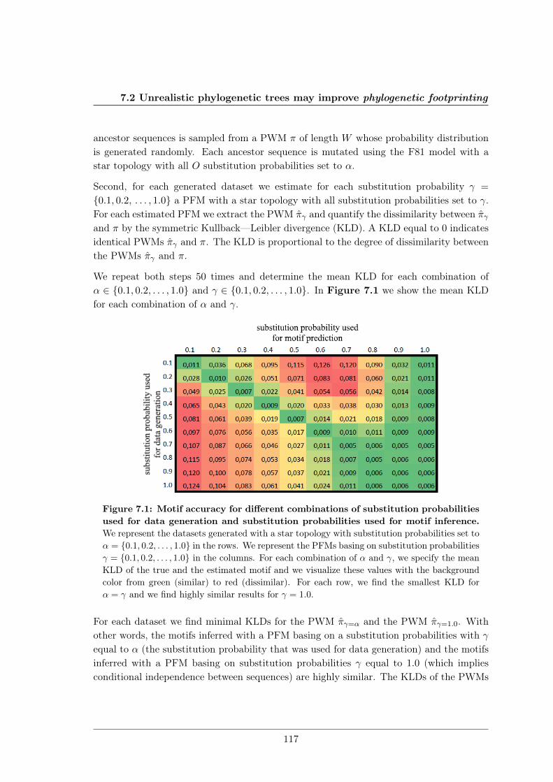
7.2 Unrealistic phylogenetic trees may improve phylogenetic footprinting

ancestor sequences is sampled from a PWM π of length W whose probability distributionis generated randomly. Each ancestor sequence is mutated using the F81 model with astar topology with all O substitution probabilities set to α.

Second, for each generated dataset we estimate for each substitution probability γ =

{0.1, 0.2, . . . , 1.0} a PFM with a star topology with all substitution probabilities set to γ.For each estimated PFM we extract the PWM πγ and quantify the dissimilarity between πγand π by the symmetric Kullback—Leibler divergence (KLD). A KLD equal to 0 indicatesidentical PWMs πγ and π. The KLD is proportional to the degree of dissimilarity betweenthe PWMs πγ and π.

We repeat both steps 50 times and determine the mean KLD for each combination ofα ∈ {0.1, 0.2, . . . , 1.0} and γ ∈ {0.1, 0.2, . . . , 1.0}. In Figure 7.1 we show the mean KLDfor each combination of α and γ.

Figure 7.1: Motif accuracy for different combinations of substitution probabilitiesused for data generation and substitution probabilities used for motif inference.We represent the datasets generated with a star topology with substitution probabilities set toα = {0.1, 0.2, . . . , 1.0} in the rows. We represent the PFMs basing on substitution probabilitiesγ = {0.1, 0.2, . . . , 1.0} in the columns. For each combination of α and γ, we specify the meanKLD of the true and the estimated motif and we visualize these values with the backgroundcolor from green (similar) to red (dissimilar). For each row, we find the smallest KLD forα = γ and we find highly similar results for γ = 1.0.

For each dataset we find minimal KLDs for the PWM πγ=α and the PWM πγ=1.0. Withother words, the motifs inferred with a PFM basing on a substitution probabilities with γequal to α (the substitution probability that was used for data generation) and the motifsinferred with a PFM basing on substitution probabilities γ equal to 1.0 (which impliesconditional independence between sequences) are highly similar. The KLDs of the PWMs

117

Page 128

7. APPENDIX

πγ with γ 6= α and γ 6= 1.0 are greater than or equal to the KLDs for the PWMs πγ=α andπγ=1.0 in every case.

7.2.1.2 Test on real data

In the previous study on synthetic data we have shown that the PWM inferred using themost realistic PFM (πγ=α) and the PWM inferred using the most unrealistic PFM (πγ=1.0)are most similar. We study whether this relationship is also true in case of real data. Incase of real data we do not know the true α, i.e., the substitution probability between theancestor species and the observed species–specific sequences. Hence, we compare the PWMπ1.0 with the PWMs πγ for γ ∈ {0.05, 0.1, . . . , 1.0}. Again, we quantify the dissimilaritybetween π1.0 and πγ by the symmetric KLD.

For each of the five TFs described in Methods 1 and each decomposition of the 100–foldstratified repeated random sub–sampling validation procedures described in Methods 4,we calculate the KLDs of the PWM π1.0 and the PWMs πγ for γ ∈ {0.05, 0.1, . . . , 1.0}inferred on the positive training dataset. We compute mean and standard error of theresulting 100 KLDs for each pair of the the PWM π1.0 and the PWMs πγ . We show meanand standard error of the KLDs as function of γ in Figure 7.2 for each of the five TFs.Based on the previous study and the results presented by Gertz et. al 2006 (Gertz et al.,2006), we expect a local minimum of the KLDs for 0.1 < γ ≤ 0.4.

We find for each TF a local minimum of the KLD between the PWM π1.0 and the PWMπγ for realistic substitution probabilities 0.1 < γ ≤ 0.4 (γ = 0.35 for CTCF, γ = 0.3 forGABP, γ = 0.25 for NRSF, γ = 0.4 for SRF, γ = 0.35 for STAT1). For γ smaller thanthese minimums the KLD increases monotonically and for γ greater than these minimumsthe KLD first increases, reaches a local maximum for 0.6 ≤ γ ≤ 0.7, and again decreasesfor γ greater this local maximum (with a KLD equal to zero for γ = 1.0 per definition). Inaccordance to the results on synthetic data, we show that the motifs inferred using a PFMbasing on unrealistic substitution probabilities are similar to the motifs inferred using aPFM basing on realistic substitution probabilities. Since the true substitution probabilitiesare not known in case of real data, the estimation of motifs using an unrealistic PFM is apotential more robust way to avoid errors from falsely estimated substitution probabilities,i.e., unrealistic PFMs seem to be more robust against model violations in the dataset.

7.2.2 Synthetic tests

In the main manuscript, we show that PFMs with unrealistic substitution probabilitiesoutperform realistic PFMs on real data in contrast to synthetic data. Here, we investigate

118

Page 129

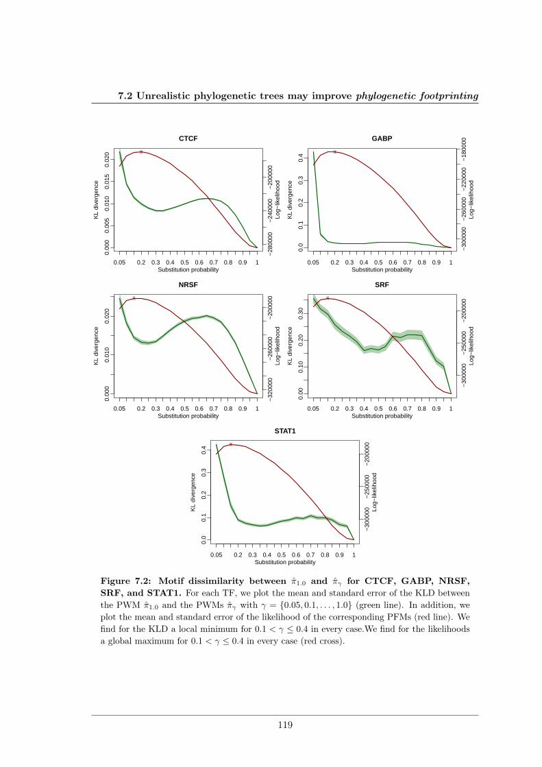
7.2 Unrealistic phylogenetic trees may improve phylogenetic footprinting0.

000

0.00

50.

010

0.01

50.

020

Substitution probability

KL

dive

rgen

ce

0.05 0.2 0.3 0.4 0.5 0.6 0.7 0.8 0.9 1

CTCF

−28

0000

−24

0000

−20

0000

Log−

likel

ihoo

d

x

0.0

0.1

0.2

0.3

0.4

Substitution probability

KL

dive

rgen

ce

0.05 0.2 0.3 0.4 0.5 0.6 0.7 0.8 0.9 1

GABP

−30

0000

−26

0000

−22

0000

−18

0000

Log−

likel

ihoo

d

x

0.00

00.

010

0.02

0

Substitution probability

KL

dive

rgen

ce

0.05 0.2 0.3 0.4 0.5 0.6 0.7 0.8 0.9 1

NRSF

−32

0000

−26

0000

−20

0000

Log−

likel

ihoo

d

x0.

000.

100.

200.

30

Substitution probability

KL

dive

rgen

ce

0.05 0.2 0.3 0.4 0.5 0.6 0.7 0.8 0.9 1

SRF

−30

0000

−25

0000

−20

0000

Log−

likel

ihoo

d

x

0.0

0.1

0.2

0.3

0.4

Substitution probability

KL

dive

rgen

ce

0.05 0.2 0.3 0.4 0.5 0.6 0.7 0.8 0.9 1

STAT1

−30

0000

−25

0000

−20

0000

Log−

likel

ihoo

d

x

Figure 7.2: Motif dissimilarity between π1.0 and πγ for CTCF, GABP, NRSF,SRF, and STAT1. For each TF, we plot the mean and standard error of the KLD betweenthe PWM π1.0 and the PWMs πγ with γ = {0.05, 0.1, . . . , 1.0} (green line). In addition, weplot the mean and standard error of the likelihood of the corresponding PFMs (red line). Wefind for the KLD a local minimum for 0.1 < γ ≤ 0.4 in every case.We find for the likelihoodsa global maximum for 0.1 < γ ≤ 0.4 in every case (red cross).

119

Page 130

7. APPENDIX

the influence of various data properties on classification performance in order to reproducethis observation on synthetic data.

We generate synthetic datasets as described in Methods 2 and modify this procedurein different ways as follows. We vary the ratio of the size of positive and negative testdata in section 7.2.2.1, we use different trees for data generation instead of a star insection 7.2.2.2, we model heterogeneity during data generation in section 7.2.2.3, weuse the more realistic HKY evolutionary model instead of the F81 model for data generationin section 7.2.2.4, and we use different trees in combination with the more realistic HKYevolutionary model for data generation in section 7.2.2.5. All datasets are available athttps://github.com/mgledi/PhyFoo/tree/master/data/synthetic_data/.

We apply the PFMs described in Methods 1 on each of the generated datasets withvarying substitution probability γ of the PFMs from 0.05 to 1.0 with increments of 0.05as described in Methods 3. We study the classification performance of the PFMs by themethod described in Methods 4.

7.2.2.1 Unbalanced positive and negative test data

120

Page 131

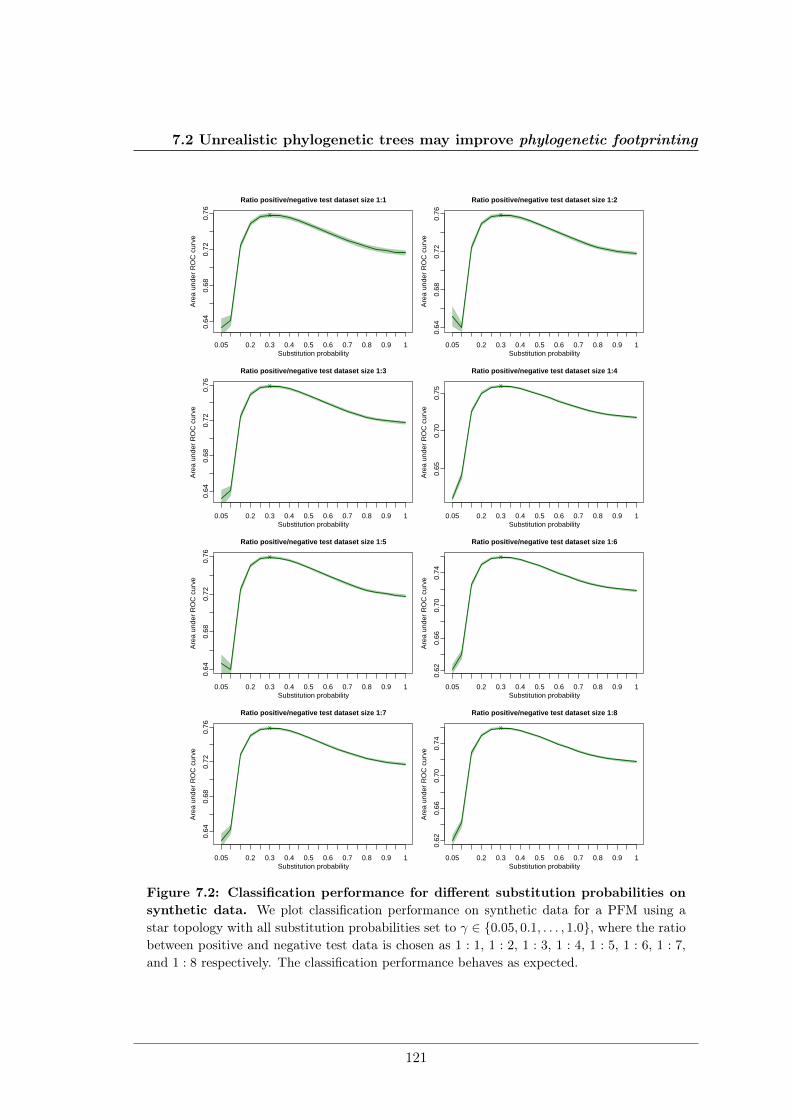
7.2 Unrealistic phylogenetic trees may improve phylogenetic footprinting

0.64

0.68

0.72

0.76

Substitution probability

Are

a un

der

RO

C c

urve

0.05 0.2 0.3 0.4 0.5 0.6 0.7 0.8 0.9 1

Ratio positive/negative test dataset size 1:1

x

0.64

0.68

0.72

0.76

Substitution probability

Are

a un

der

RO

C c

urve

0.05 0.2 0.3 0.4 0.5 0.6 0.7 0.8 0.9 1

Ratio positive/negative test dataset size 1:2

x

0.64

0.68

0.72

0.76

Substitution probability

Are

a un

der

RO

C c

urve

0.05 0.2 0.3 0.4 0.5 0.6 0.7 0.8 0.9 1

Ratio positive/negative test dataset size 1:3

x

0.65

0.70

0.75

Substitution probability

Are

a un

der

RO

C c

urve

0.05 0.2 0.3 0.4 0.5 0.6 0.7 0.8 0.9 1

Ratio positive/negative test dataset size 1:4

x

0.64

0.68

0.72

0.76

Substitution probability

Are

a un

der

RO

C c

urve

0.05 0.2 0.3 0.4 0.5 0.6 0.7 0.8 0.9 1

Ratio positive/negative test dataset size 1:5

x

0.62

0.66

0.70

0.74

Substitution probability

Are

a un

der

RO

C c

urve

0.05 0.2 0.3 0.4 0.5 0.6 0.7 0.8 0.9 1

Ratio positive/negative test dataset size 1:6

x

0.64

0.68

0.72

0.76

Substitution probability

Are

a un

der

RO

C c

urve

0.05 0.2 0.3 0.4 0.5 0.6 0.7 0.8 0.9 1

Ratio positive/negative test dataset size 1:7

x

0.62

0.66

0.70

0.74

Substitution probability

Are

a un

der

RO

C c

urve

0.05 0.2 0.3 0.4 0.5 0.6 0.7 0.8 0.9 1

Ratio positive/negative test dataset size 1:8

x

Figure 7.2: Classification performance for different substitution probabilities onsynthetic data. We plot classification performance on synthetic data for a PFM using astar topology with all substitution probabilities set to γ ∈ {0.05, 0.1, . . . , 1.0}, where the ratiobetween positive and negative test data is chosen as 1 : 1, 1 : 2, 1 : 3, 1 : 4, 1 : 5, 1 : 6, 1 : 7,and 1 : 8 respectively. The classification performance behaves as expected.

121

Page 132

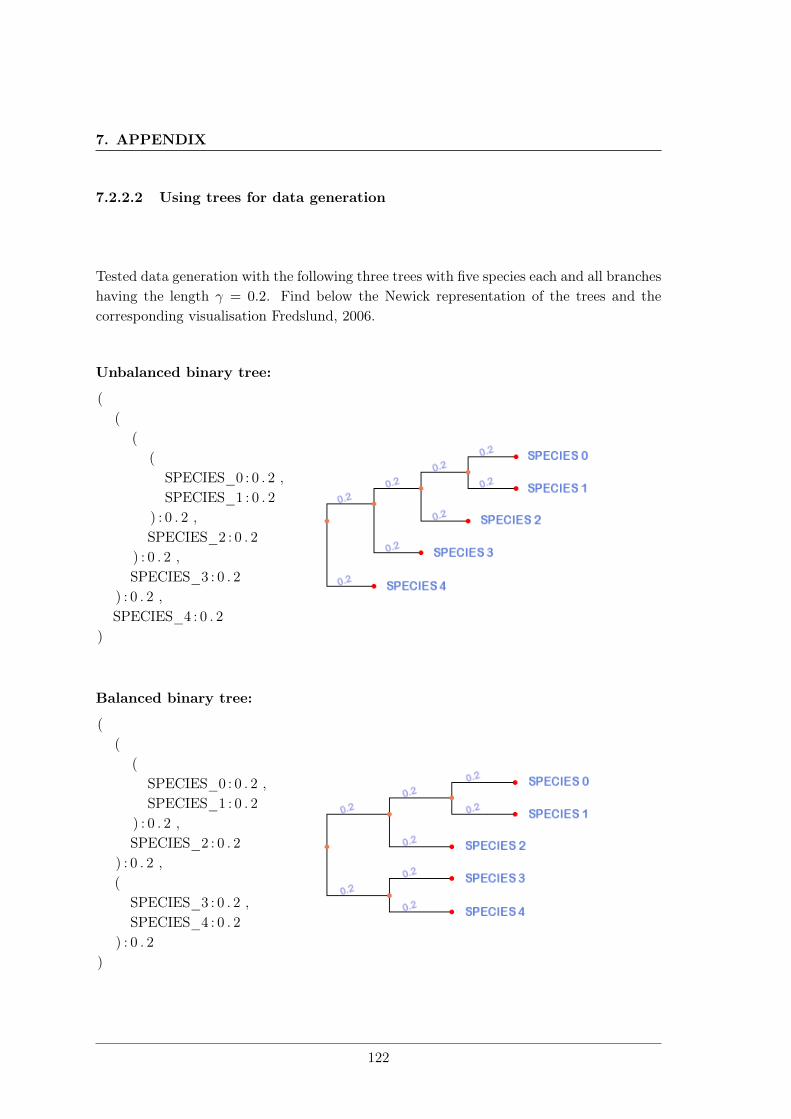
7. APPENDIX

7.2.2.2 Using trees for data generation

Tested data generation with the following three trees with five species each and all brancheshaving the length γ = 0.2. Find below the Newick representation of the trees and thecorresponding visualisation Fredslund, 2006.

Unbalanced binary tree:

((

((

SPECIES_0 : 0 . 2 ,SPECIES_1 : 0 . 2

) : 0 . 2 ,SPECIES_2 : 0 . 2

) : 0 . 2 ,SPECIES_3 : 0 . 2

) : 0 . 2 ,SPECIES_4 : 0 . 2

)

Balanced binary tree:

((

(SPECIES_0 : 0 . 2 ,SPECIES_1 : 0 . 2

) : 0 . 2 ,SPECIES_2 : 0 . 2

) : 0 . 2 ,(

SPECIES_3 : 0 . 2 ,SPECIES_4 : 0 . 2

) : 0 . 2)

122

Page 133

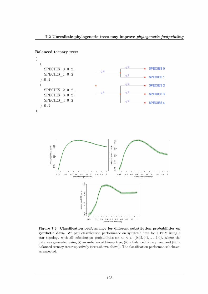
7.2 Unrealistic phylogenetic trees may improve phylogenetic footprinting

Balanced ternary tree:

((

SPECIES_0 : 0 . 2 ,SPECIES_1 : 0 . 2

) : 0 . 2 ,(

SPECIES_2 : 0 . 2 ,SPECIES_3 : 0 . 2 ,SPECIES_4 : 0 . 2

) : 0 . 2)

0.75

0.80

0.85

Substitution probability

Are

a un

der

RO

C c

urve

0.05 0.2 0.3 0.4 0.5 0.6 0.7 0.8 0.9 1

x

0.78

0.80

0.82

0.84

0.86

Substitution probability

Are

a un

der

RO

C c

urve

0.05 0.2 0.3 0.4 0.5 0.6 0.7 0.8 0.9 1

x

0.54

0.58

0.62

0.66

Substitution probability

Are

a un

der

RO

C c

urve

0.05 0.2 0.3 0.4 0.5 0.6 0.7 0.8 0.9 1

x

Figure 7.3: Classification performance for different substitution probabilities onsynthetic data. We plot classification performance on synthetic data for a PFM using astar topology with all substitution probabilities set to γ ∈ {0.05, 0.1, . . . , 1.0}, where thedata was generated using (i) an unbalanced binary tree, (ii) a balanced binary tree, and (iii) abalanced ternary tree respectively (trees shown above). The classification performance behavesas expected.

123

Page 134

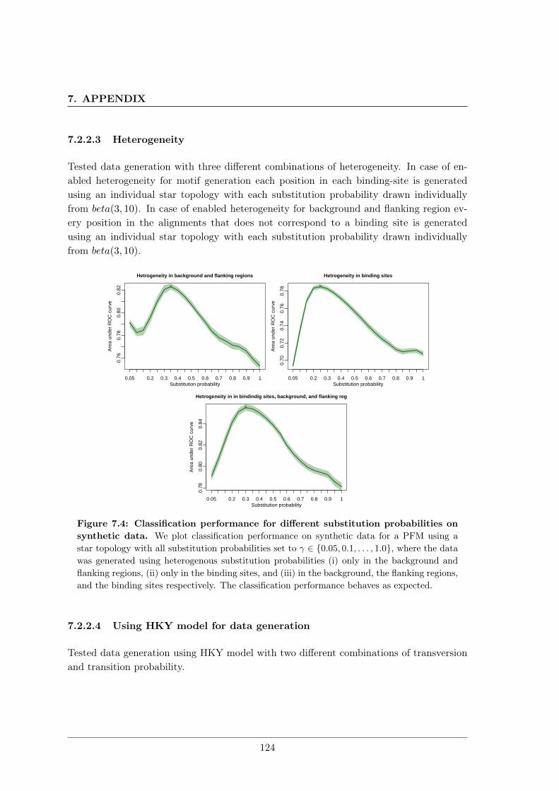
7. APPENDIX

7.2.2.3 Heterogeneity

Tested data generation with three different combinations of heterogeneity. In case of en-abled heterogeneity for motif generation each position in each binding-site is generatedusing an individual star topology with each substitution probability drawn individuallyfrom beta(3, 10). In case of enabled heterogeneity for background and flanking region ev-ery position in the alignments that does not correspond to a binding site is generatedusing an individual star topology with each substitution probability drawn individuallyfrom beta(3, 10).

0.76

0.78

0.80

0.82

Substitution probability

Are

a un

der

RO

C c

urve

0.05 0.2 0.3 0.4 0.5 0.6 0.7 0.8 0.9 1

Hetrogeneity in background and flanking regions

x0.

700.

720.

740.

760.

78

Substitution probability

Are

a un

der

RO

C c

urve

0.05 0.2 0.3 0.4 0.5 0.6 0.7 0.8 0.9 1

Hetrogeneity in binding sites

x

0.78

0.80

0.82

0.84

Substitution probability

Are

a un

der

RO

C c

urve

0.05 0.2 0.3 0.4 0.5 0.6 0.7 0.8 0.9 1

Hetrogeneity in in bindindig sites, background, and flanking regions

x

Figure 7.4: Classification performance for different substitution probabilities onsynthetic data. We plot classification performance on synthetic data for a PFM using astar topology with all substitution probabilities set to γ ∈ {0.05, 0.1, . . . , 1.0}, where the datawas generated using heterogenous substitution probabilities (i) only in the background andflanking regions, (ii) only in the binding sites, and (iii) in the background, the flanking regions,and the binding sites respectively. The classification performance behaves as expected.

7.2.2.4 Using HKY model for data generation

Tested data generation using HKY model with two different combinations of transversionand transition probability.

124

Page 135

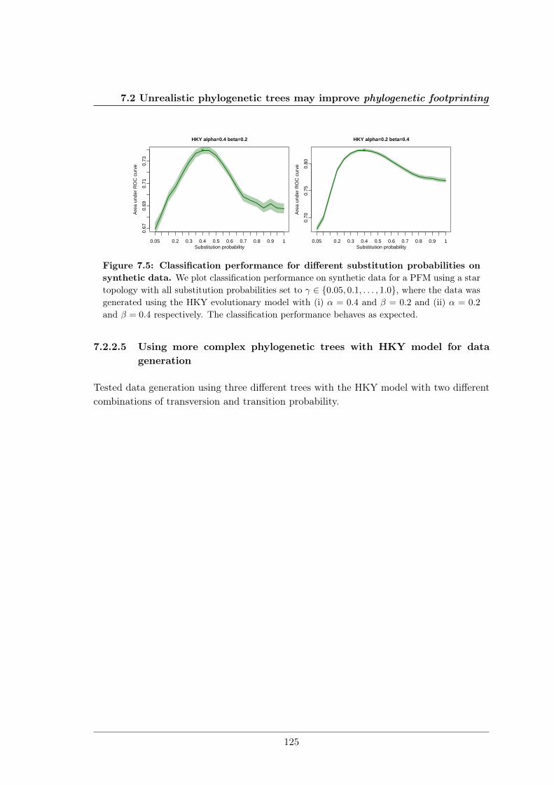
7.2 Unrealistic phylogenetic trees may improve phylogenetic footprinting

0.67

0.69

0.71

0.73

Substitution probability

Are

a un

der

RO

C c

urve

0.05 0.2 0.3 0.4 0.5 0.6 0.7 0.8 0.9 1

HKY alpha=0.4 beta=0.2

x

0.70

0.75

0.80

Substitution probability

Are

a un

der

RO

C c

urve

0.05 0.2 0.3 0.4 0.5 0.6 0.7 0.8 0.9 1

HKY alpha=0.2 beta=0.4

x

Figure 7.5: Classification performance for different substitution probabilities onsynthetic data. We plot classification performance on synthetic data for a PFM using a startopology with all substitution probabilities set to γ ∈ {0.05, 0.1, . . . , 1.0}, where the data wasgenerated using the HKY evolutionary model with (i) α = 0.4 and β = 0.2 and (ii) α = 0.2

and β = 0.4 respectively. The classification performance behaves as expected.

7.2.2.5 Using more complex phylogenetic trees with HKY model for datageneration

Tested data generation using three different trees with the HKY model with two differentcombinations of transversion and transition probability.

125

Page 136

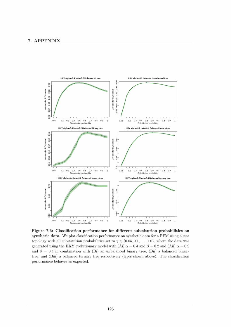
7. APPENDIX

0.80

0.82

0.84

0.86

0.88

0.90

Substitution probability

Are

a un

der

RO

C c

urve

0.05 0.2 0.3 0.4 0.5 0.6 0.7 0.8 0.9 1

HKY alpha=0.4 beta=0.2 Unbalanced tree

x

0.86

0.88

0.90

0.92

0.94

0.96

Substitution probability

Are

a un

der

RO

C c

urve

0.05 0.2 0.3 0.4 0.5 0.6 0.7 0.8 0.9 1

HKY alpha=0.2 beta=0.4 Unbalanced tree

x

0.56

0.58

0.60

0.62

0.64

0.66

Substitution probability

Are

a un

der

RO

C c

urve

0.05 0.2 0.3 0.4 0.5 0.6 0.7 0.8 0.9 1

HKY alpha=0.4 beta=0.2 Balanced binary tree

x

0.80

0.84

0.88

0.92

Substitution probability

Are

a un

der

RO

C c

urve

0.05 0.2 0.3 0.4 0.5 0.6 0.7 0.8 0.9 1

HKY alpha=0.2 beta=0.4 Balanced binary tree

x

0.58

0.62

0.66

0.70

Substitution probability

Are

a un

der

RO

C c

urve

0.05 0.2 0.3 0.4 0.5 0.6 0.7 0.8 0.9 1

HKY alpha=0.4 beta=0.2 Balanced ternery tree

x

0.80

0.84

0.88

Substitution probability

Are

a un

der

RO

C c

urve

0.05 0.2 0.3 0.4 0.5 0.6 0.7 0.8 0.9 1

HKY alpha=0.2 beta=0.4 Balanced ternery tree

x

Figure 7.6: Classification performance for different substitution probabilities onsynthetic data. We plot classification performance on synthetic data for a PFM using a startopology with all substitution probabilities set to γ ∈ {0.05, 0.1, . . . , 1.0}, where the data wasgenerated using the HKY evolutionary model with (Ai) α = 0.4 and β = 0.2 and (Aii) α = 0.2

and β = 0.4 in combination with (Bi) an unbalanced binary tree, (Bii) a balanced binarytree, and (Biii) a balanced ternary tree respectively (trees shown above). The classificationperformance behaves as expected.

126

Page 137

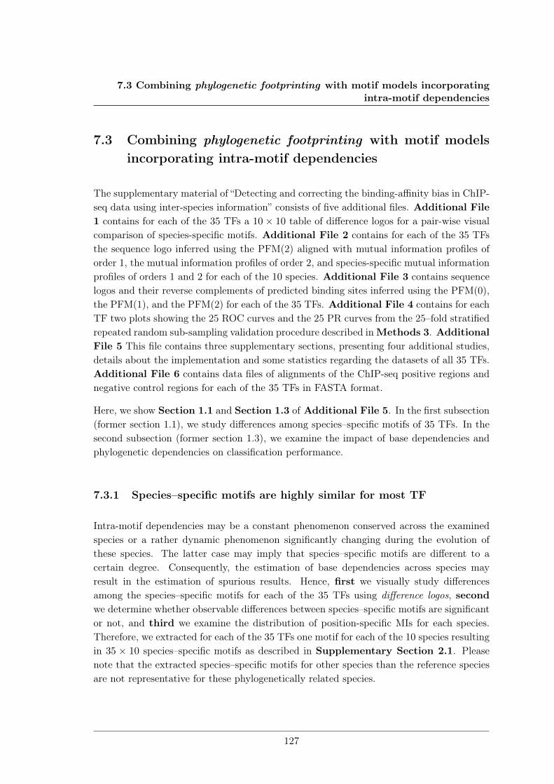
7.3 Combining phylogenetic footprinting with motif models incorporatingintra-motif dependencies

7.3 Combining phylogenetic footprinting with motif modelsincorporating intra-motif dependencies

The supplementary material of “Detecting and correcting the binding-affinity bias in ChIP-seq data using inter-species information” consists of five additional files. Additional File1 contains for each of the 35 TFs a 10× 10 table of difference logos for a pair-wise visualcomparison of species-specific motifs. Additional File 2 contains for each of the 35 TFsthe sequence logo inferred using the PFM(2) aligned with mutual information profiles oforder 1, the mutual information profiles of order 2, and species-specific mutual informationprofiles of orders 1 and 2 for each of the 10 species. Additional File 3 contains sequencelogos and their reverse complements of predicted binding sites inferred using the PFM(0),the PFM(1), and the PFM(2) for each of the 35 TFs. Additional File 4 contains for eachTF two plots showing the 25 ROC curves and the 25 PR curves from the 25–fold stratifiedrepeated random sub-sampling validation procedure described inMethods 3. AdditionalFile 5 This file contains three supplementary sections, presenting four additional studies,details about the implementation and some statistics regarding the datasets of all 35 TFs.Additional File 6 contains data files of alignments of the ChIP-seq positive regions andnegative control regions for each of the 35 TFs in FASTA format.

Here, we show Section 1.1 and Section 1.3 of Additional File 5. In the first subsection(former section 1.1), we study differences among species–specific motifs of 35 TFs. In thesecond subsection (former section 1.3), we examine the impact of base dependencies andphylogenetic dependencies on classification performance.

7.3.1 Species–specific motifs are highly similar for most TF

Intra-motif dependencies may be a constant phenomenon conserved across the examinedspecies or a rather dynamic phenomenon significantly changing during the evolution ofthese species. The latter case may imply that species–specific motifs are different to acertain degree. Consequently, the estimation of base dependencies across species mayresult in the estimation of spurious results. Hence, first we visually study differencesamong the species–specific motifs for each of the 35 TFs using difference logos, secondwe determine whether observable differences between species–specific motifs are significantor not, and third we examine the distribution of position-specific MIs for each species.Therefore, we extracted for each of the 35 TFs one motif for each of the 10 species resultingin 35 × 10 species–specific motifs as described in Supplementary Section 2.1. Pleasenote that the extracted species–specific motifs for other species than the reference speciesare not representative for these phylogenetically related species.

127

Page 138

7. APPENDIX

7.3.1.1 Primates show almost no differences in their sequence logos

We use the freely available R package DiffLogo for the visual inspection of motif differencesNettling, Treutler, Grau, et al., 2015. DiffLogo enables the illustration and investigation ofdifferences between highly similar motifs such as binding motifs of TFs from different ex-periments, different motif prediction algorithms, or different species. Hence, we use tablesof difference logos generated with DiffLogo for a pair-wise comparison of all species–specificmotifs. Each difference logo displays position-specific differences of base distributions bya stack of bases which height is proportional to the base distribution difference quantifiedby the Jensen-Shannon divergence. The Jensen-Shannon divergence is zero in case of twoidentical base distributions and 1 in case of two maximally different base distributions. Thetables of difference logos for all 35 TFs can be found in Additional File 1. All sequencelogos of PFM(0), PFM(1), and PFM(2) can be found in Additional File 3.

Exemplary, Supplementary Figure 7.7 shows the table of difference logos for the TFBach1. We find that the species–specific motifs segregate into two main groups, where onegroup comprises seven higher primates and the second group comprises three species fromthe Laurasiatheria superorder, i.e., dog, horse, and cow. We find differences between themotifs of both groups at various motif positions, where the motif differences of relativelyhigh degree are located at rather conserved motif positions as well as at more variablemotif positions. For instance, we find relatively high differences at motif position 8, whereguanine is more abundant in the primate motifs and the remaining bases are more abundantin the Laurasiatheria motifs. However, the maximum Jensen-Shannon divergence in alldifference logos for Bach1 is below 0.01 bits.

We examine the motif differences between species–specific motifs for all 35 TFs. We see for14 TFs that the set of ten species segregates into the two groups of seven higher primatesand three from the Laurasiatheria clade as before in case of Bach1 (CEBPB, CTCF, EGR1,MafK, Max, NRSF, POU5F1, Rad21, SRF, TCF12, TEAD4, USF1, USF2, YY1). We findfor the remaining 21 TFs that the motifs of the seven higher primates are more similarto each other compared to the motifs of dog, horse, and cow. With other words, in thesecases the pairwise difference logos of dog, horse, and cow do not form a second cluster. Thedifferences observed among species–specific motifs could partly result from missing bindingsites in some species. Supplementary Table S6 shows for each species and for each TFthe proportion of sequences which are available for the computation of species–specificmotifs.

128

Page 139

7.3 Combining phylogenetic footprinting with motif models incorporatingintra-motif dependencies

Figure 7.7: Comparison of species-specific motifs for the TF Bach1. We depicta table of difference logos with one row and one column for each species-specific motif toemphasize the differences between species-specific motifs. Each difference logos depicts themotif differences position-wise with a stack of bases, which height is calculated by the Jensen-Shannon divergence of the position-specific base distributions. The overall similarity betweenspecies-specific motifs is calculated by the sum of Jensen-Shannon divergences of all motifpositions and depicted by the background color of the difference logos from green (similar) tored (dissimilar). The table of difference logos indicates, that the ten species-specific Bach1motifs primarily segregate into two clusters, where one cluster comprises seven primates andthe other cluster comprises three non-primates (cow, dog, and horse).

7.3.1.2 Species–specific motifs are typically highly similar

We study the statistical significance of differences between species–specific motifs as follows.We examine for each of the 35 TFs the similarity of species–specific motifs using a statisticaltest for each two species ((10 ∗ 9)/2 = 45 species pairs). We calculate for each TF andfor each two species the p-value for the null hypothesis that two species–specific motifsarise from the same distribution as described in Supplementary Section 2.2 resultingin 35 ∗ 45 = 1575 pairwise comparisons. We count for each two species how often we rejectthe null hypothesis for a confidence level of α = 0.05. These counts range from 0 to 35,

129

Page 140

7. APPENDIX

where 0 means that the species-specific motifs of two species show no significant differencesfor each transcription factor and 35 means that the species-specific motifs of two speciesshow significant differences for each transcription factor. The binary nature of the resultsof statistical tests can lead to the issue that comparisons between three species are nottransitive, i.e., if there are no significant differences between the species–specific motifsof species A and B and there are no significant differences between the species–specificmotifs of species B and C it can happen that there are significant differences between thespecies–specific motifs of species A and C.

Supplementary Table S3 shows the results for each pair of species. We find that theseven primate-specific motifs are highly similar to each other and that the three species-specific motifs of cow, dog, and horse show greater differences compared to those of theseven primates. Using a significance level of 95%, we expect 5% of all 1575 pairwisedifferences to be significant by chance. We find for only 47 of 1575 pairwise comparisonsthat two species–specific motifs show significant differences. However, we find only 47 (3%)of the pairwise differences to be significant, stating that the observed differences are notgreater than expected by chance.

Specifically, we find that these 47 cases apply only to 6 of the 35 TFs, namely Bach1,CEBPB, MafK, Max, SP1, and USF1 and typically only apply to comparisons betweena primate species and one of the species dog, cow, and horse. We find no significantdifferences between the seven primates reflecting the close phylogenetic relationship andaccordingly the high sequence similarity. Amongst the three species dog, cow, and horsewe find for 1 of the 105 pairwise comparisons significant differences.

These results imply that the motifs estimated across species as presented in the previoussection are typically not a mixture of species–specific motifs.

7.3.1.3 Intra–motif dependencies are highly similar for all species

We examine for each of the 35 TFs the distribution of species–specific MIs using mutualinformation profiles IS1 and IS2 as described in Methods 4 for each species S ∈ {hg19,panTro, papHam, ponAbe, rheMac, calJac, equCab, canFam, gorGor, bosTau}. Fig-ure 7.8 shows two examples of species–specific mutual information profiles IS1 and IS2 forthe two TFs CJUN and Nrf. All species–specific mutual information profiles are availablein Additional File 2.

First, we study the species–specific mutual information profiles IS1 . We find for each ofthe 35 TFs that the species–specific mutual information profiles IS1 are highly similar forall species. We also find that the MIs in the mutual information profiles I1 are sometimesstronger, sometimes weaker, and often averaged compared to the species–specific MIs IS1

130

Page 141

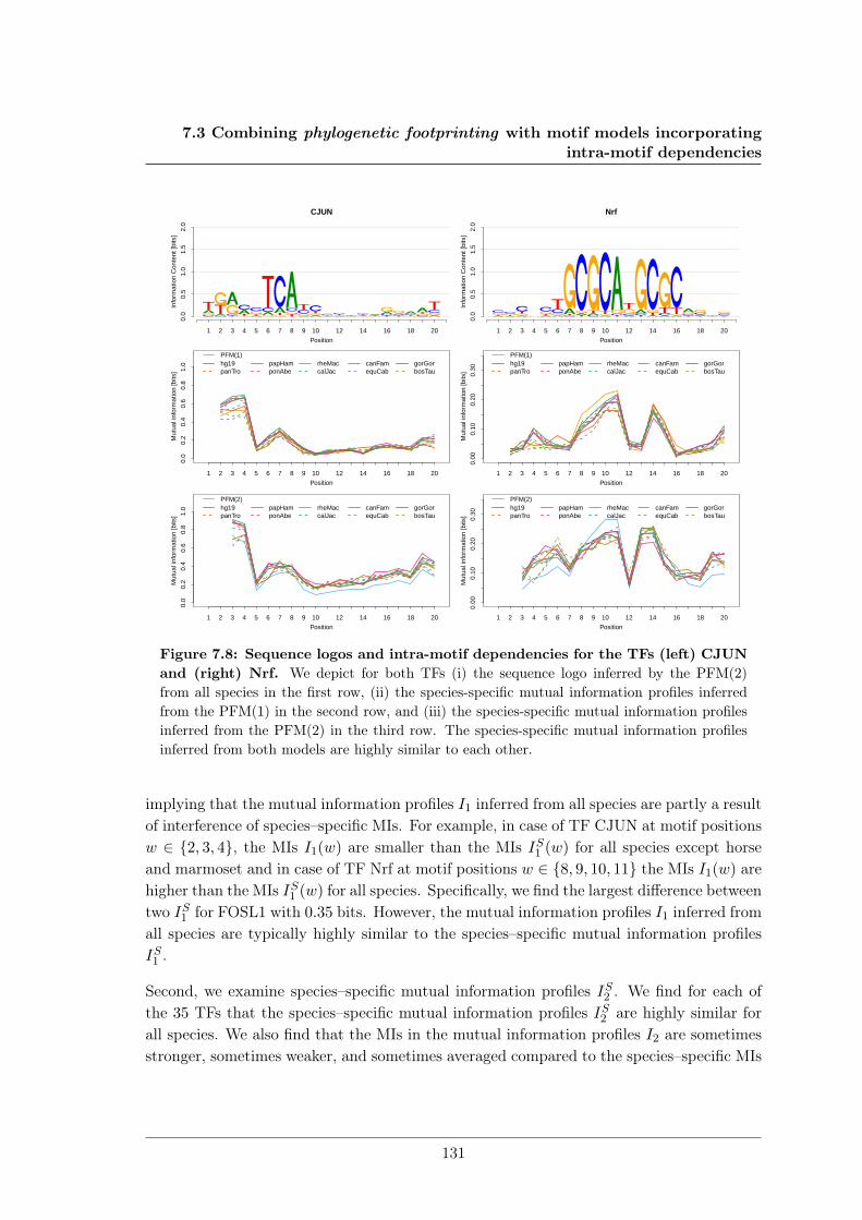
7.3 Combining phylogenetic footprinting with motif models incorporatingintra-motif dependencies

0.0

0.5

1.0

1.5

2.0

Position

Info

rmat

ion

Con

tent

[bits

]

1 2 3 4 5 6 7 8 9 10 12 14 16 18 20

CJUN

●

0.0

0.2

0.4

0.6

Position

Mut

ual i

nfor

mat

ion

[bits

]

1 2 3 4 5 6 7 8 9 10 12 14 16 18 20

●

● ●

●

●

●

●

●

●● ● ●

●

● ● ●●

● ●

●●

●

●

● ●

●

●●

● ● ●

●●

●

●

●

●

PFM(1) PFM(2)

●

0.0

0.2

0.4

0.6

0.8

1.0

Position

Mut

ual i

nfor

mat

ion

[bits

]

1 2 3 4 5 6 7 8 9 10 12 14 16 18 20

hg19panTro

papHamponAbe

rheMaccalJac

canFamequCab

gorGorbosTau

PFM(1)

0.0

0.2

0.4

0.6

0.8

1.0

Position

Mut

ual i

nfor

mat

ion

[bits

]

1 2 3 4 5 6 7 8 9 10 12 14 16 18 20

hg19panTro

papHamponAbe

rheMaccalJac

canFamequCab

gorGorbosTau

PFM(2)

0.0

0.5

1.0

1.5

2.0

Position

Info

rmat

ion

Con

tent

[bits

]

1 2 3 4 5 6 7 8 9 10 12 14 16 18 20

CJUN

●

0.0

0.2

0.4

0.6

Position

Mut

ual i

nfor

mat

ion

[bits

]

1 2 3 4 5 6 7 8 9 10 12 14 16 18 20

●

● ●

●

●

●

●

●

●● ● ●

●

● ● ●●

● ●

●●

●

●

● ●

●

●●

● ● ●

●●

●

●

●

●

PFM(1) PFM(2)

●

0.0

0.2

0.4

0.6

0.8

1.0

Position

Mut

ual i

nfor

mat

ion

[bits

]

1 2 3 4 5 6 7 8 9 10 12 14 16 18 20

hg19panTro

papHamponAbe

rheMaccalJac

canFamequCab

gorGorbosTau

PFM(1)

0.0

0.2

0.4

0.6

0.8

1.0

Position

Mut

ual i

nfor

mat

ion

[bits

]

1 2 3 4 5 6 7 8 9 10 12 14 16 18 20

hg19panTro

papHamponAbe

rheMaccalJac

canFamequCab

gorGorbosTau

PFM(2)

0.0

0.5

1.0

1.5

2.0

Position

Info

rmat

ion

Con

tent

[bits

]

1 2 3 4 5 6 7 8 9 10 12 14 16 18 20

Nrf

0.00

0.10

0.20

0.30

Position

Mut

ual i

nfor

mat

ion

[bits

]

1 2 3 4 5 6 7 8 9 10 12 14 16 18 20

●●

●

● ●●

●

●

●●

● ●

●

●

●

● ●●

●

●

●●

●

●

●

●

● ●

●

● ●

●

●

●●

● ●

PFM(1) PFM(2)

0.00

0.10

0.20

0.30

Position

Mut

ual i

nfor

mat

ion

[bits

]

1 2 3 4 5 6 7 8 9 10 12 14 16 18 20

hg19panTro

papHamponAbe

rheMaccalJac

canFamequCab

gorGorbosTau

PFM(1)

0.00

0.10

0.20

0.30

Position

Mut

ual i

nfor

mat

ion

[bits

]

1 2 3 4 5 6 7 8 9 10 12 14 16 18 20

hg19panTro

papHamponAbe

rheMaccalJac

canFamequCab

gorGorbosTau

PFM(2)

0.0

0.5

1.0

1.5

2.0

Position

Info

rmat

ion

Con

tent

[bits

]

1 2 3 4 5 6 7 8 9 10 12 14 16 18 20

Nrf

0.00

0.10

0.20

0.30

Position

Mut

ual i

nfor

mat

ion

[bits

]

1 2 3 4 5 6 7 8 9 10 12 14 16 18 20

●●

●

● ●●

●

●

●●

● ●

●

●

●

● ●●

●

●

●●

●

●

●

●

● ●

●

● ●

●

●

●●

● ●

PFM(1) PFM(2)

0.00

0.10

0.20

0.30

Position

Mut

ual i

nfor

mat

ion

[bits

]

1 2 3 4 5 6 7 8 9 10 12 14 16 18 20

hg19panTro

papHamponAbe

rheMaccalJac

canFamequCab

gorGorbosTau

PFM(1)

0.00

0.10

0.20

0.30

Position

Mut

ual i

nfor

mat

ion

[bits

]

1 2 3 4 5 6 7 8 9 10 12 14 16 18 20

hg19panTro

papHamponAbe

rheMaccalJac

canFamequCab

gorGorbosTau

PFM(2)

Figure 7.8: Sequence logos and intra-motif dependencies for the TFs (left) CJUNand (right) Nrf. We depict for both TFs (i) the sequence logo inferred by the PFM(2)from all species in the first row, (ii) the species-specific mutual information profiles inferredfrom the PFM(1) in the second row, and (iii) the species-specific mutual information profilesinferred from the PFM(2) in the third row. The species-specific mutual information profilesinferred from both models are highly similar to each other.

implying that the mutual information profiles I1 inferred from all species are partly a resultof interference of species–specific MIs. For example, in case of TF CJUN at motif positionsw ∈ {2, 3, 4}, the MIs I1(w) are smaller than the MIs IS1 (w) for all species except horseand marmoset and in case of TF Nrf at motif positions w ∈ {8, 9, 10, 11} the MIs I1(w) arehigher than the MIs IS1 (w) for all species. Specifically, we find the largest difference betweentwo IS1 for FOSL1 with 0.35 bits. However, the mutual information profiles I1 inferred fromall species are typically highly similar to the species–specific mutual information profilesIS1 .

Second, we examine species–specific mutual information profiles IS2 . We find for each ofthe 35 TFs that the species–specific mutual information profiles IS2 are highly similar forall species. We also find that the MIs in the mutual information profiles I2 are sometimesstronger, sometimes weaker, and sometimes averaged compared to the species–specific MIs

131

Page 142

7. APPENDIX

IS2 implying that the mutual information profiles I2 inferred from all species are partly aresult of interference of species–specific MIs. For example, in case of CJUN the mutualinformation profile I2(w) is typically smaller than the mutual information profile IS2 (w) forall species at all motif positions w and in case of Nrf at motif positions w ∈ {8−11} the MIsI2(w) are higher than the MIs IS2 (w). Specifically, we find the largest difference betweentwo IS2 for FOSL1 with 0.48 bits. However, the mutual information profiles I2 inferred fromall species are typically highly similar to the species–specific mutual information profilesIS2 as in case of I1 and IS1 .

132

Page 143

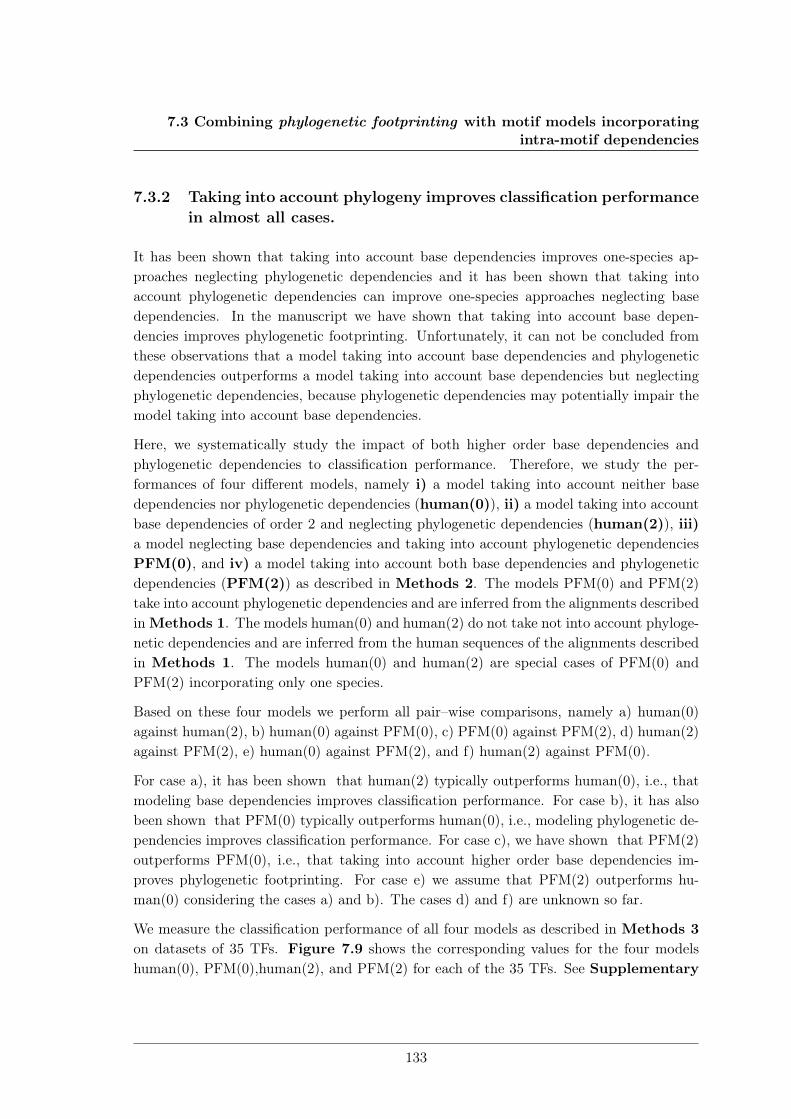
7.3 Combining phylogenetic footprinting with motif models incorporatingintra-motif dependencies

7.3.2 Taking into account phylogeny improves classification performancein almost all cases.

It has been shown that taking into account base dependencies improves one-species ap-proaches neglecting phylogenetic dependencies and it has been shown that taking intoaccount phylogenetic dependencies can improve one-species approaches neglecting basedependencies. In the manuscript we have shown that taking into account base depen-dencies improves phylogenetic footprinting. Unfortunately, it can not be concluded fromthese observations that a model taking into account base dependencies and phylogeneticdependencies outperforms a model taking into account base dependencies but neglectingphylogenetic dependencies, because phylogenetic dependencies may potentially impair themodel taking into account base dependencies.

Here, we systematically study the impact of both higher order base dependencies andphylogenetic dependencies to classification performance. Therefore, we study the per-formances of four different models, namely i) a model taking into account neither basedependencies nor phylogenetic dependencies (human(0)), ii) a model taking into accountbase dependencies of order 2 and neglecting phylogenetic dependencies (human(2)), iii)a model neglecting base dependencies and taking into account phylogenetic dependenciesPFM(0), and iv) a model taking into account both base dependencies and phylogeneticdependencies (PFM(2)) as described in Methods 2. The models PFM(0) and PFM(2)take into account phylogenetic dependencies and are inferred from the alignments describedinMethods 1. The models human(0) and human(2) do not take not into account phyloge-netic dependencies and are inferred from the human sequences of the alignments describedin Methods 1. The models human(0) and human(2) are special cases of PFM(0) andPFM(2) incorporating only one species.

Based on these four models we perform all pair–wise comparisons, namely a) human(0)against human(2), b) human(0) against PFM(0), c) PFM(0) against PFM(2), d) human(2)against PFM(2), e) human(0) against PFM(2), and f) human(2) against PFM(0).

For case a), it has been shown that human(2) typically outperforms human(0), i.e., thatmodeling base dependencies improves classification performance. For case b), it has alsobeen shown that PFM(0) typically outperforms human(0), i.e., modeling phylogenetic de-pendencies improves classification performance. For case c), we have shown that PFM(2)outperforms PFM(0), i.e., that taking into account higher order base dependencies im-proves phylogenetic footprinting. For case e) we assume that PFM(2) outperforms hu-man(0) considering the cases a) and b). The cases d) and f) are unknown so far.

We measure the classification performance of all four models as described in Methods 3on datasets of 35 TFs. Figure 7.9 shows the corresponding values for the four modelshuman(0), PFM(0),human(2), and PFM(2) for each of the 35 TFs. See Supplementary

133

Page 144

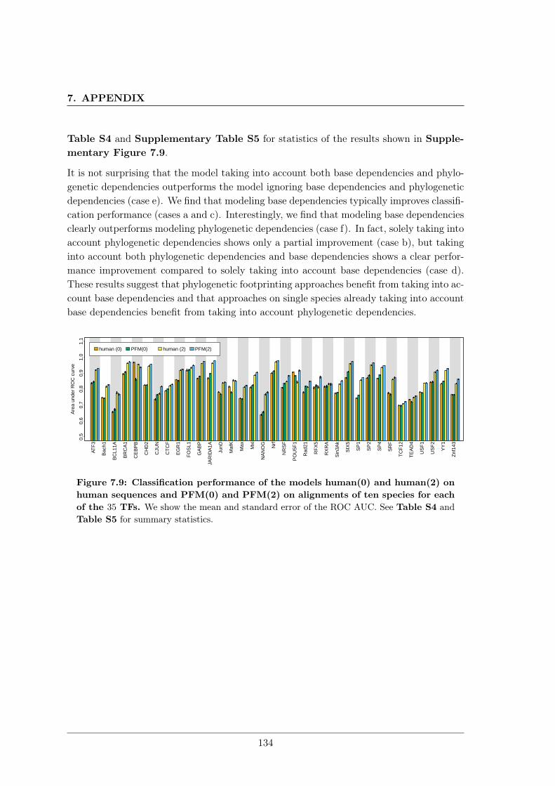
7. APPENDIX

Table S4 and Supplementary Table S5 for statistics of the results shown in Supple-mentary Figure 7.9.

It is not surprising that the model taking into account both base dependencies and phylo-genetic dependencies outperforms the model ignoring base dependencies and phylogeneticdependencies (case e). We find that modeling base dependencies typically improves classifi-cation performance (cases a and c). Interestingly, we find that modeling base dependenciesclearly outperforms modeling phylogenetic dependencies (case f). In fact, solely taking intoaccount phylogenetic dependencies shows only a partial improvement (case b), but takinginto account both phylogenetic dependencies and base dependencies shows a clear perfor-mance improvement compared to solely taking into account base dependencies (case d).These results suggest that phylogenetic footprinting approaches benefit from taking into ac-count base dependencies and that approaches on single species already taking into accountbase dependencies benefit from taking into account phylogenetic dependencies.

ATF

3

Bac

h1

BC

L11A

BR

CA

1

CE

BP

B

CH

D2

CJU

N

CT

CF

EG

R1

FO

SL1

GA

BP

JAR

IDA

1A

JunD

Maf

K

Max Mxi

NA

NO

G Nrf

NR

SF

PO

U5F

1

Rad

21

RF

X5

RX

RA

Sin

3Ak

SIX

5

SP

1

SP

2

SP

4

SR

F

TC

F12

TE

AD

4

US

F1

US

F2

YY

1

Znf

143

0.5

0.6

0.7

0.8

0.9

1.0

1.1

Are

a un

der

RO

C c

urve

human (0) PFM(0) human (2) PFM(2)

Figure 7.9: Classification performance of the models human(0) and human(2) onhuman sequences and PFM(0) and PFM(2) on alignments of ten species for eachof the 35 TFs. We show the mean and standard error of the ROC AUC. See Table S4 andTable S5 for summary statistics.

134

Page 145

7.3 Combining phylogenetic footprinting with motif models incorporatingintra-motif dependencies

ATF

3

Bac

h1

BC

L11A

BR

CA

1

CE

BP

B

CH

D2

CJU

N

CT

CF

EG

R1

FO

SL1

GA

BP

JAR

IDA

1A

JunD

Maf

K

Max Mxi

NA

NO

G Nrf

NR

SF

PO

U5F

1

Rad

21

RF

X5

RX

RA

Sin

3Ak

SIX

5

SP

1

SP

2

SP

4

SR

F

TC

F12

TE

AD

4

US

F1

US

F2

YY

1

Znf

143

−60

−40

−20

020

4060

Rel

ativ

e in

crea

se o

f RO

C A

UC

[%] PFM(0) rel. to human(0)

ATF

3

Bac

h1

BC

L11A

BR

CA

1

CE

BP

B

CH

D2

CJU

N

CT

CF

EG

R1

FO

SL1

GA

BP

JAR

IDA

1A

JunD

Maf

K

Max Mxi

NA

NO

G Nrf

NR

SF

PO

U5F

1

Rad

21

RF

X5

RX

RA

Sin

3Ak

SIX

5

SP

1

SP

2

SP

4

SR

F

TC

F12

TE

AD

4

US

F1

US

F2

YY

1

Znf

143

−40

−20

020

4060

Rel

ativ

e in

crea

se o

f RO

C A

UC

[%] PFM(2) rel. to human(2)

Figure 7.10: Classification performance of the two models PFM(0) and PFM(2)incorporating phylogenetic dependencies for each of the 35 TFs. We show the meanand standard error of the relative increase of ROC AUC of (top) PFM(0) relative to theclassification performance of human(0) and (bottom) PFM(2) relative to the classificationperformance of human(2). Typically both models show a higher classification performance.

135

Page 146

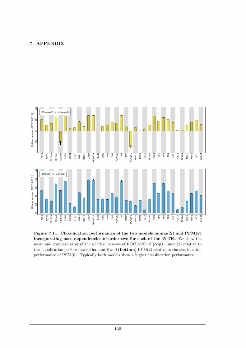
7. APPENDIXAT

F3

Bac

h1

BC

L11A

BR

CA

1

CE

BP

B

CH

D2

CJU

N

CT

CF

EG

R1

FO

SL1

GA

BP

JAR

IDA

1A

JunD

Maf

K

Max Mxi

NA

NO

G Nrf

NR

SF

PO

U5F

1

Rad

21

RF

X5

RX

RA

Sin

3Ak

SIX

5

SP

1

SP

2

SP

4

SR

F

TC

F12

TE

AD

4

US

F1

US

F2

YY

1

Znf

143

−50

050

100

Rel

ativ

e in

crea

se o

f RO

C A

UC

[%] human(2) rel. to human(0)

ATF

3

Bac

h1

BC

L11A

BR

CA

1

CE

BP

B

CH

D2

CJU

N

CT

CF

EG

R1

FO

SL1

GA

BP

JAR

IDA

1A

JunD

Maf

K

Max Mxi

NA

NO

G Nrf

NR

SF

PO

U5F

1

Rad

21

RF

X5

RX

RA

Sin

3Ak

SIX

5

SP

1

SP

2

SP

4

SR

F

TC

F12

TE

AD

4

US

F1

US

F2

YY

1

Znf

143

020

4060

8010

0

Rel

ativ

e in

crea

se o

f RO

C A

UC

[%] PFM(2) rel. to PFM(0)

Figure 7.11: Classification performance of the two models human(2) and PFM(2)incorporating base dependencies of order two for each of the 35 TFs. We show themean and standard error of the relative increase of ROC AUC of (top) human(2) relative tothe classification performance of human(0) and (bottom) PFM(2) relative to the classificationperformance of PFM(0). Typically both models show a higher classification performance.

136

Page 147

7.4 DiffLogo: A comparative visualisation of sequence motifs

7.4 DiffLogo: A comparative visualisation of sequence mo-tifs

The supplementary material of “DiffLogo: a comparative visualization of sequence motifs”consists of one additional file that contains Supplementary Methods, Results, Figures, andExamples. This file comprises four sections. Section 1, Additional examples, containsFigures S1 and S2. In Section 2, CTCF with and without clustering, we show in detailthe impact of clustering and optimal leaf ordering for a DiffLogo grid of nine CTCF motifs.In Section 3, Alternative combinations of stack heights and symbol weights, we describethe mathematical background of four implementations of H` and two implementationsof r`,a and show an exemplary comparison of the eight combinations. In Section 4,Tool comparison, we compare DiffLogo with the five tools seqLogo, iceLogo, MotifStack,STAMP, and Two Sample Logo. Here, I provide a copy of Section 3.

7.4.1 Alternative combinations of stack heights and symbol weights

We consider two motifs represented by two PWMs p and q. The height of symbol a in thesymbol stack at position ` of the difference logo is denoted H`,a and given by

H`,a = r`,a ·H`,

where H` represents the height of the symbol stack at position ` and the weight r`,arepresents the proportion of symbol a ∈ A in the symbol stack at position `, where A isthe alphabet. We calculate H`,a for different measures H` and r`,a to emphasize differentfacets of distribution differences. We propose various alternatives to calculate the measuresH` and r`,a as follows (illustrated in supplementary Table S1.

In the following sections, the information content of a PWM p at position ` is denoted Hp`

and given by

Hp` = log2(|A|)−

∑a∈A

p`,a · log2(p`,a),

where p`,a is the probability of symbol a at position ` in PWM p. Hq` is defined analo-

gously.

7.4.1.1 Different calculations of stack heights H`

Jensen–Shannon divergence

137

Page 148

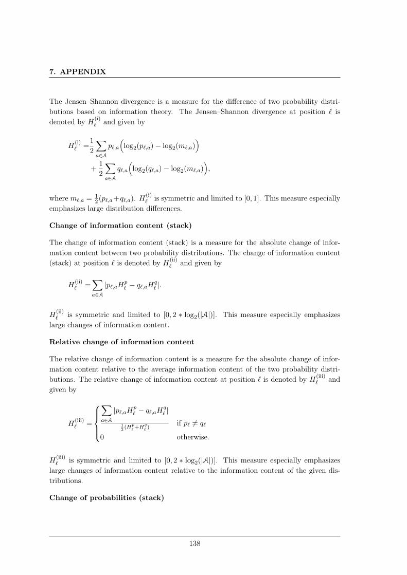
7. APPENDIX

The Jensen–Shannon divergence is a measure for the difference of two probability distri-butions based on information theory. The Jensen–Shannon divergence at position ` isdenoted by H(i)

` and given by

H(i)` =

1

2

∑a∈A

p`,a

(log2(p`,a)− log2(m`,a)

)+

1

2

∑a∈A

q`,a

(log2(q`,a)− log2(m`,a)

),

where m`,a =12(p`,a+q`,a). H

(i)` is symmetric and limited to [0, 1]. This measure especially

emphasizes large distribution differences.

Change of information content (stack)

The change of information content (stack) is a measure for the absolute change of infor-mation content between two probability distributions. The change of information content(stack) at position ` is denoted by H(ii)

` and given by

H(ii)` =

∑a∈A|p`,aHp

` − q`,aHq` |.

H(ii)` is symmetric and limited to [0, 2 ∗ log2(|A|)]. This measure especially emphasizes

large changes of information content.

Relative change of information content

The relative change of information content is a measure for the absolute change of infor-mation content relative to the average information content of the two probability distri-butions. The relative change of information content at position ` is denoted by H(iii)

` andgiven by

H(iii)` =

∑a∈A|p`,aHp

` − q`,aHq` |

12(Hp

`+Hq` )

if p` 6= q`

0 otherwise.

H(iii)` is symmetric and limited to [0, 2 ∗ log2(|A|)]. This measure especially emphasizes

large changes of information content relative to the information content of the given dis-tributions.

Change of probabilities (stack)

138

Page 149

7.4 DiffLogo: A comparative visualisation of sequence motifs

The change of probabilities (stack) is a measure for the absolute change of probabilitiesbetween two probability distributions. The change of probabilities (stack) at position ` isdenoted by H(iv)

` and given by

H(iv)` =

∑a∈A|p`,a − q`,a|

H(iv)` is symmetric and limited to [0, 2]. This measure especially emphasizes large changes

of probabilities.

7.4.1.2 Different calculations of symbol weights r`,a

Change of probability (symbol)

The change of probability (symbol) is a measure for the change of symbol-specific prob-ability relative to the sum of absolute symbol-specific probability differences of the givenprobability distributions. The change of probability (symbol) of symbol a at position ` isdenoted by r(i)`,a and given by

r(i)`,a =

p`,a−q`,a∑

a′∈A |p`,a′−q`,a′ |if p` 6= q`

0 otherwise.

r(i)`,a is antisymmetric and limited to [−1

2 ,12 ]. This measure especially emphasizes a large

change of symbol–probability. For each position of the difference logo, the height of thesymbol stack with negative measures r(i)`,a is equal to the height of the symbol stack with

positive measures r(i)`,a, because each gain of symbol–probability implies a loss of probabilityfor the remaining symbols and vice versa.

Change of information content (symbol)

The change of information content (symbol) is a measure for the symbol-specific changeof information content relative to the sum of absolute symbol-specific differences of infor-mation content of the given probability distributions. The change of information content(symbol) of symbol a at position ` is denoted by r(ii)`,a and given by

r(ii)`,a =

p`,aH

p`−q`,aH

q`∑

a∈A |p`,aHp`−q`,aH

q` |

if p` 6= q`

0 otherwise.

r(ii)`,a is antisymmetric and limited to [−1, 1]. This measure especially emphasizes a largechange of symbol-specific information content.

139

Page 150

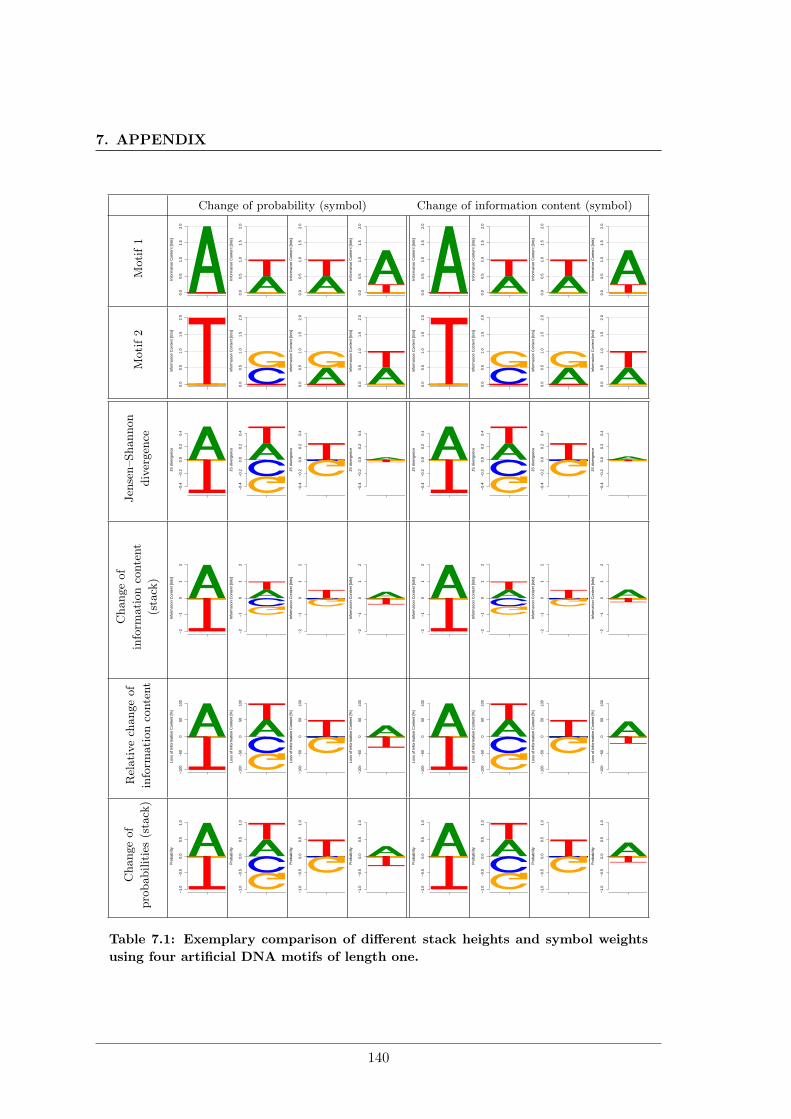
7. APPENDIX

Change of probability (symbol) Change of information content (symbol)

Motif1

0.0

0.5

1.0

1.5

2.0

Position

Info

rmat

ion

Con

tent

[bits

]

1

0.0

0.5

1.0

1.5

2.0

Position

Info

rmat

ion

Con

tent

[bits

]

10.

00.

51.

01.

52.

0

Position

Info

rmat

ion

Con

tent

[bits

]

1

0.0

0.5

1.0

1.5

2.0

Position

Info

rmat

ion

Con

tent

[bits

]

1

0.0

0.5

1.0

1.5

2.0

Position

Info

rmat

ion

Con

tent

[bits

]

1

0.0

0.5

1.0

1.5

2.0

Position

Info

rmat

ion

Con

tent

[bits

]

1

0.0

0.5

1.0

1.5

2.0

Position

Info

rmat

ion

Con

tent

[bits

]

1

0.0

0.5

1.0

1.5

2.0

Position

Info

rmat

ion

Con

tent

[bits

]

1

Motif2

0.0

0.5

1.0

1.5

2.0

Position

Info

rmat

ion

Con

tent

[bits

]

1

0.0

0.5

1.0

1.5

2.0

Position

Info

rmat

ion

Con

tent

[bits

]

1

0.0

0.5

1.0

1.5

2.0

Position

Info

rmat

ion

Con

tent

[bits

]

1

0.0

0.5

1.0

1.5

2.0

Position

Info

rmat

ion

Con

tent

[bits

]

1

0.0

0.5

1.0

1.5

2.0

Position

Info

rmat

ion

Con

tent

[bits

]

1

0.0

0.5

1.0

1.5

2.0

Position

Info

rmat

ion

Con

tent

[bits

]

1

0.0

0.5

1.0

1.5

2.0

Position

Info

rmat

ion

Con

tent

[bits

]

1

0.0

0.5

1.0

1.5

2.0

Position

Info

rmat

ion

Con

tent

[bits

]

1

Jensen

–Sha

nnon

divergen

ce

−0.

4−

0.2

0.0

0.2

0.4

Position

JS d

iver

genc

e

1

−0.

4−

0.2

0.0

0.2

0.4

Position

JS d

iver

genc

e

1

−0.

4−

0.2

0.0

0.2

0.4

Position

JS d

iver

genc

e

1

−0.

4−

0.2

0.0

0.2

0.4

Position

JS d

iver

genc

e

1

−0.

4−

0.2

0.0

0.2

0.4

Position

JS d

iver

genc

e

1

−0.

4−

0.2

0.0

0.2

0.4

Position

JS d

iver

genc

e

1

−0.

4−

0.2

0.0

0.2

0.4

Position

JS d

iver

genc

e

1

−0.

4−

0.2

0.0

0.2

0.4

Position

JS d

iver

genc

e

1

Cha

ngeof

inform

ationcontent

(stack)

−2

−1

01

2

Position

Info

rmat

ion

Con

tent

[bits

]

1

−2

−1

01

2

Position

Info

rmat

ion

Con

tent

[bits

]

1

−2

−1

01

2

Position

Info

rmat

ion

Con

tent

[bits

]

1

−2

−1

01

2

Position

Info

rmat

ion

Con

tent

[bits

]

1

−2

−1

01

2

Position

Info

rmat

ion

Con

tent

[bits

]

1

−2

−1

01

2

Position

Info

rmat

ion

Con

tent

[bits

]

1

−2

−1

01

2

Position

Info

rmat

ion

Con

tent

[bits

]

1

−2

−1

01

2

Position

Info

rmat

ion

Con

tent

[bits

]

1

Relativechan

geof

inform

ationcontent

−10

0−

500

5010

0

Position

Loss

of I

nfor

mat

ion

Con

tent

[%]

1

−10

0−

500

5010

0

Position

Loss

of I

nfor

mat

ion

Con

tent

[%]

1

−10

0−

500

5010

0

Position

Loss

of I

nfor

mat

ion

Con

tent

[%]

1

−10

0−

500

5010

0

Position

Loss

of I

nfor

mat

ion

Con

tent

[%]

1

−10

0−

500

5010

0

Position

Loss

of I

nfor

mat

ion

Con

tent

[%]

1

−10

0−

500

5010

0

Position

Loss

of I

nfor

mat

ion

Con

tent

[%]

1

−10

0−

500

5010

0

Position

Loss

of I

nfor

mat

ion

Con

tent

[%]

1

−10

0−

500

5010

0

Position

Loss

of I

nfor

mat

ion

Con

tent

[%]

1

Cha

ngeof

prob

abilities

(stack)

−1.

0−

0.5

0.0

0.5

1.0

Position

Pro

babi

lity

1

−1.

0−

0.5

0.0

0.5

1.0

Position

Pro

babi

lity

1

−1.

0−

0.5

0.0

0.5

1.0

Position

Pro

babi

lity

1

−1.

0−

0.5

0.0

0.5

1.0

Position

Pro

babi

lity

1

−1.

0−

0.5

0.0

0.5

1.0

Position

Pro

babi

lity

1

−1.

0−

0.5

0.0

0.5

1.0

Position

Pro

babi

lity

1

−1.

0−

0.5

0.0

0.5

1.0

Position

Pro

babi

lity

1

−1.

0−

0.5

0.0

0.5

1.0

Position

Pro

babi

lity

1

Table 7.1: Exemplary comparison of different stack heights and symbol weightsusing four artificial DNA motifs of length one.

140

Page 151

Eidesstattliche Erklärung / Declaration under Oath

Ich erkläre an Eides statt, dass ich die Arbeit sebstständig und ohne fremde Hilfe verfasst,keine anderen als die von mir angegegebenen Quellen und Hilfsmittel benutzt und dieden benutzten Werken wörtlich oder inhaltlich entnommenen Stellen als solche kenntlichgemacht habe.

I declare under penalty of perjury that this thesis is my own work entirely and has beenwritten without any help from other people. I used only the sources mentioned and includedall the citations correctly both in word or content.

Burgliebenau, 15.05.2017 Martin Nettling

Page 152

Page 153

Martin Nettling

Phone: +49 173 360 12 83 | [email protected]

Page 1

Personal

information

Address

Die Mühlbreite 21

06258 Burgliebenau

Date of birth, birth name

10.06.1982, Gleditzsch

Nationality

German

Family status

married, two kids

Education

07/2008 Diploma Bioinformatics

Martin-Luther-University, Halle/Wittenberg

06/2001 Abitur

European school in Waldenburg

Professional

experience

01/2016 – today

Senior Software Engineer Research and Development

Datameer GmbH, Halle

» Development of distributed algorithms

» Development of Elasticsearch plugins

08/2012 – 10/2015

Teamlead Research and Development

Unister GmbH, Leipzig

» Analysis and interpretation of large data sets

» Development of distributed algorithms

» Leading a team of up to six team members

10/2010 – 07/2012

Junior Developer Machine-Learning

Unister GmbH, Leipzig

» Implementation of algorithms for text analysis

» Performance optimization of existing implementations

11/2003 – 06/2007

Developer of the CMS of the MLU Halle/Wittenberg

» Conception and backend development

Page 154

Martin Nettling

Phone: +49 173 360 12 83 | [email protected]

Page 2

Publications

Articles

M Nettling, H Treutler, J Cerquides, I Grosse. 2016. Unrealistic

phylogenetic trees may improve phylogenetic footprinting.

Bioinformatics, accepted

M Nettling, H Treutler, J Cerquides, I Grosse. 2016. Combining

phylogenetic footprinting with motif models incorporating intra-motif

dependencies.

BMC bioinformatics, accepted

M Nettling, H Treutler, J Cerquides, I Grosse. 2016. Detecting and

correcting the binding-affinity bias in ChIP-Seq data using inter-species

information. BMC genomics 17:1.

M Nettling*, H Treutler*, J Grau, J Keilwagen, S Posch, I Grosse.

2015. DiffLogo: a comparative visualization of sequence motifs. BMC

Bioinformatics, 16:1

M Nettling, N Thieme, A Both, I Grosse. 2014. DRUMS: Disk

Repository with Update Management and Select option for high

throughput sequencing data. BMC bioinformatics, 15:1.

P Alexiou, T Vergoulis, M Gleditzsch, G Prekas, T Dalamagas, M

Megraw, I Grosse, T Sellis, AG Hatzigeorgiou. 2009. miRGen 2.0: a

database of microRNA genomic information and regulation. Nucl. Acids

Res. 38 (suppl 1): D137-D141

Conference papers

L Avdiyenko, M Nettling, C Lemke, M Wauer, ACN Ngomo, A Both.

(2015) Motive-based search: Computing regions from large knowledge

bases using geospatial coordinates. International Joint Conference on

Knowledge Engineering and Knowledge Management (IC3K), (Vol. 1,

pp. 469-474). SCITEPRESS.

M Wauer, A Both, S Schwinger, M Nettling, O Erling. (2015)

Integrating custom index extensions into virtuoso RDF store for e-

commerce applications. Proceedings of the 11th International

Conference on Semantic Systems (pp. 65-72). ACM.

F Rosner, A Hinneburg, M Röder, M Nettling, A Both. (2013)

Evaluating topic coherence measures. arXiv preprint arXiv:1403.6397.

F Rosner, A Hinneburg, M Gleditzsch, M Priebe, A Both. (2012) Fast

sampling word correlations of high dimensional text data. Proceedings

of the 2012 ACM SIGMOD International Conference on Management of

Data (pp. 866-866). ACM.

Page 155

Martin Nettling

Phone: +49 173 360 12 83 | [email protected]

Page 3

Open source

software

» DRUMS: Disk repository with update management

and select option

https://github.com/mgledi/DRUMS

» BioDRUMS: Example integration of

DRUMS for biological data

https://github.com/mgledi/BioDRUMS

» DiffLogo: Comparative visualization of sequence motifs in R

https://github.com/mgledi/DiffLogo

» DiffLogoUI: A webserver for DiffLogo

https://github.com/mgledi/DiffLogoUI

Burgliebenau, 01.12.2016 Martin Nettling