Nevada Division of Environmental Protection Bureau of … for Hydrogeologic Groundwater Flow Modeling at Mine Sites Prepared by Connor P. Newman 22 March 2018 1. Introduction Mining

901 S. Stewart Street, Suite 4001 • Carson City, Nevada 89701 • p: 775.687.4670 • f: 775.687.5856 • ndep.nv.gov Printed on recycled paper

Nevada Division of Environmental Protection

Bureau of Mining Regulation and Reclamation

Guidance for Hydrogeologic Groundwater Flow Modeling at Mine Sites

Prepared by

Connor P. Newman

22 March 2018

1. Introduction

Mining operations in the State of Nevada commonly interact with local and regional groundwater, due to

groundwater pumping for dewatering, groundwater rebound, pit-lake formation, infiltration of excess

water, and various other processes. The complexity of these interactions often necessitates the use of

groundwater flow models to predict future conditions quantitatively, and the Nevada Division of

Environmental Protection, Bureau of Mining Regulation and Reclamation (the Division) may require

groundwater models during permitting actions. This guidance document summarizes the background and

general requirements for groundwater flow modeling studies submitted to the Division. This guidance is

not intended to include all possible requirements, and may need periodic updates as scientific

understanding and groundwater modeling methods evolve. The guidance document provides a reference

for Division employees, mining operators and consultants, and other users/reviewers of groundwater flow

models, and is intended to decrease the number of technical comments associated with groundwater

models, thereby increasing permitting efficiency and decreasing permitting time.

In its most basic definition, a model is a simplification of a physical system. A groundwater flow model

specifically is a simplification of the groundwater system of interest, and is meant to be used for a specific

purpose (BLM, 2008; Reilly and Harbaugh, 2004). When required by the Division, groundwater flow

models are intended to be used to assess possible future impacts to the waters of the State, as regulated in

the Nevada Administrative Code (NAC) 445A.424 and 445A.429.

Not every mining operation is required to conduct groundwater modeling, because not all mining

operations have the potential to impact waters of the State. Examples of mining operations not typically

required to perform groundwater modeling include small-scale placer operations and mines not interacting

with groundwater (i.e., no degradation, pumping, infiltration, pit lakes, etc.), or where more simple data

analyses suffice. However, other regulatory agencies including the Nevada Division of Water Resources

(NDWR), the United States Forest Service (USFS), and the United States Bureau of Land Management

(BLM) may have other permitting requirements. Mine operators are encouraged to contact all applicable

agencies for their regulatory requirements. All groundwater models for regulated mining operations

should be submitted to the Division for review.

Nevada Division of Environmental Protection Bureau of Mining Regulation and Reclamation


Revision 00 22 March 2018

Page 2 of 28

P:\BMRR\PublicDocs\Guidance Docs and Forms Reg and Closure\Modeling\Final\201803_CPN_Hydro_Guidance_revision00.docx

Site-specific Division requirements for groundwater flow modeling, if any, for mining operations already

holding a water pollution control permit (WPCP) are commonly described in the WPCP. Whether required

specifically by the WPCP or otherwise by the Division, all groundwater flow models submitted to the

Division must adhere to general requirements set forth herein. This guidance is not intended to be overly

prescriptive, however, as to the exact content, layout, and design of groundwater flow modeling and model

reports. Not every process discussed in this document will be applicable at every site, and additional

processes may warrant investigation at specific sites. This guidance is not meant to stifle innovation with

respect to the methods and analyses utilized in groundwater modeling. Instead the guidance is designed

to provide a reference and to describe documentation that is required for submitted groundwater models.

The goal of groundwater modeling submitted to the Division is to provide a tool that can be used to inform

policy and permitting decisions made by the Division. The results of these models may play a significant

role in assessing future impacts of proposed mine sites. Because of the weight carried by these

groundwater models and their inherent uncertainty, preparers of groundwater models have a duty to

evaluate and communicate the objectives and uncertainties of the model, as well as possible alternative

actions to reduce environmental impacts, in associated correspondence and reports (Bredehoeft, 2005;

Reilly and Harbaugh, 2004; Oreskes et al., 1994). Additionally, reviewers of groundwater models have

the duty to provide fair and reasonable reviews based on best scientific practices. Alternatives included in

model reports could include mitigation measures or other such actions. Analysis of alternatives in this

sense is different from requirements for alternatives analysis considered in National Environmental Policy

Act (NEPA) documents. In this case, alternative actions can be identified and evaluated during the

operation of the project and be instituted when required, instead of relying on a previous NEPA analysis

completed during initial permitting.

Useful summaries of the numerous complexities involved in groundwater flow modeling and model

reporting are provided in Anderson et al. (2015), Barnett et al. (2012), BLM (2008), Bredehoeft (2003;

2005), Reilly and Harbaugh (2004), groundwater modeling guidance papers distributed by the National

Groundwater Association (NGWA; http://www.ngwa.org/pubs/Pages/white-papers.aspx), and various

ASTM International documents. Modelers should be keenly aware of common modeling errors, such as

those summarized at the conclusion of each chapter of Anderson et al. (2015). These listings of common

errors should prove especially useful, as the Division has encountered many of these errors in submitted

groundwater model reports.

2. Groundwater Modeling Methods

There are various types of groundwater flow models, and each type has associated input data, assumed

parameters, and model outputs. One major distinction amongst types of groundwater models is analytical

models versus numerical models. In general, analytical solutions are simpler to solve, are continuous in

time and space, and require less input data. In contrast, numerical models are more complex and solve the

governing equations of groundwater flow for discrete points in space and in time (Anderson et al., 2015).

The majority of groundwater flow models provided to the Division are numerical models. Numerical

models may not always be the appropriate modeling method, however; in some cases, more simple

methods may provide more useful results (Kelson et al., 2002; Shevenell, 2000). Aryafar et al. (2007)

http://www.ngwa.org/pubs/Pages/white-papers.aspx




Page 3 of 28


provides a review of analytical methods in reference to calculating groundwater inflow to pit lakes and

Hunt et al. (2003) discuss various methodologies for simulating lake-groundwater interactions. In addition

to true analytical methods, the analytic element method is effective in many instances and should be

considered for mining applications. See Hunt (2006) and Strack (2003) for additional information on

analytic element methods. Groundwater modelers should consider carefully the most appropriate

modeling method, and describe the reasoning for the applied method in model reports (Reilly and

Harbaugh, 2004). An important consideration in choosing the modeling method is what questions the

groundwater model must answer (e.g., impact to stream baseflow, the water balance of a pit lake, potential

for pit-lake discharge to the downgradient aquifer, etc.). In many cases there are numerous questions asked

of a groundwater model. The questions asked, and the required resolution of the answers, should be

primary considerations when choosing the modeling method (Kelson et al., 2002). The reasoning behind

these choices and what questions the model is attempting to answer must be outlined in the modeling

report.

Much of the guidance summarized in this document is applicable to both analytical and numerical models,

but, owing to their greater complexity, numerical models are emphasized. Numerical modeling may be

further subdivided into finite-element and finite-difference methods. The differences between these

methods are beyond the scope of this document, but comparisons between both methods indicate that

similar results are obtained regardless of the numerical method (Anderson et al., 2015). The Division

accepts either numerical method.

Numerous proprietary (e.g., owned by a particular company and not open for public use and review) and

open-source groundwater modeling codes exist for both finite-difference and finite-element methods. In

the experience of the Division, the most widely used groundwater modeling code is MODFLOW

(Harbaugh, 2005), or variations of this code including MODFLOW-USG (Panday et al., 2015) and

MODFLOW SURFACT (HGL, 2002). MODFLOW and its variations are finite-difference codes

originally developed by the United States Geological Survey (USGS). MODFLOW is ideal for a variety

of reasons including: it is open-source and freely available with instruction manuals, it has been subject

to considerable internal review, and it has been utilized in numerous peer-reviewed scientific research

articles. Aside from MODFLOW, the Division has experience with other codes, both proprietary and

open-source. Until now, no official guidance has been offered by the Division on the use of proprietary

versus open-source codes.

It is the belief of the Division that proprietary codes are not appropriate for use in predictive models

impacting regulatory decisions and public or environmental health, for a variety of reasons (Nordstrom,

2012). This is not to say that some proprietary codes do not sufficiently solve groundwater flow problems

(e.g., Trefry and Muffels, 2007); however, the lack of transparency is an issue. If the modeler wishes to

use a proprietary code, or an open-source code having undocumented performance, an assessment must

be made as to the reliability of the code. Although Oreskes et al. (1994) question the term “verification”

for numerical codes, the Division believes reproducibility must be assessed and confirmed. There are

various documents relating to the testing and assurance of reliability of modeling codes (ASTM D6025-

96; van der Heijde, 1996; van der Heijde and Kanzer, 1997). Reporting of code testing should be consistent

with these documents. Once a specific code has been tested, and the testing has been approved by the

Division, the code need not be tested again by future users, unless the code has subsequently been




Page 4 of 28


modified. The Division will maintain a listing of tested codes on its website at: https://ndep.nv.gov/.

Additionally, an operational copy and instruction manual of any proprietary code must be supplied to the

Division for use in model review. The requirement for modeling to use publically available codes is

consistent with actions taken by other states; for example, see requirements for groundwater models

submitted to the California Department of Water Resources (CDWR, 2016).

Owing to the relative simplicity and variability of programming languages used in analytical models,

analytical modeling codes must be specified, but need not be verified. Any analytical modeling code used

in groundwater flow modeling must be submitted concurrent with the groundwater flow model report it

has been applied in.

3. Conceptual Models

Prior to any analytical or numerical modeling, the region to be simulated must be simplified in order to

characterize the hydrogeologic framework and define pertinent processes that must be quantitatively

incorporated into the subsequent modeling procedures. This simplification process is referred to as

conceptual model creation. The conceptual model is primarily a qualitative representation of the system

of interest and includes information on physiographic, geologic, climatologic, hydrologic, and

geochemical characteristics (Anderson et al., 2015). Conceptual models could include some quantitative

information or analysis, which help to understand the system. Although conceptual models may quickly

mature, the process should be iterative and upon additional data collection conceptual and numerical

models may need to be changed (ASTM D5979-96; Bredehoeft, 2005). Conceptual models are one of the

most important parts of the groundwater model, although they are sometimes overlooked. The iterative

processes of conceptual and numerical modeling should be used to guide additional data collection, which

will lead to a more advanced understanding of the groundwater system. Additionally, comparison of

multiple conceptual models with observations is an excellent way to test assumptions about processes

occurring at the site of interest (Bredehoeft, 2003; 2005).

It is critical that the conceptual model for the hydrogeologic system of interest be a reasonable

approximation of the system. Conceptual models should adhere to the principle of parsimony (also known

as Occam’s Razor); that is, the conceptual model should be the simplest possible description of the system

while including all relevant processes and containing enough complexity to represent important system

behavior. This concept requires that all relevant features or processes reasonably expected to occur in the

model domain are included in the conceptual model. It is also imperative for all processes included in the

conceptual model to be included in the numerical model, and vice versa. Finally, the conceptual model

must be built upon and supported by abundant and representative site-specific characterization data.

Where minor data gaps exist, which is common for groundwater modeling, appropriate substitutions may

be made. The model report must address these data gaps and provide supporting reasoning for any

substitutions. The Division may require additional data collection to fill data gaps in a specified timeframe.

Important aspects of the conceptual model include: geologic and hydrogeologic framework, sources of

groundwater recharge and discharge, groundwater flow directions, hydrogeologic discontinuities,

boundary conditions, climatologic characteristics, groundwater budget components, structural geologic

https://ndep.nv.gov/




Page 5 of 28


framework, and geochemical characteristics. The conceptual model for the site of interest should be

compared to any applicable published conceptual models and water budgets (e.g., Heilweil and Brooks,

2011), and any differences addressed. An in-depth discussion of the aspects and importance of conceptual

model formation is provided in Anderson et al. (2015), ASTM D5979-96, and Bredehoeft (2003; 2005).

Additionally, Maurer et al. (2004) and Heilweil and Brooks (2011) provide useful references for the

creation of conceptual models that are specific to Nevada.

4. Data Collection and Model Integration

In the experience of the Division, it is common for modeling exercises to reach advanced stages without

adequate characterization data, which are required per NAC 445A.395 for surface water and groundwater

quality, and NAC 445A.396 for overburden, waste rock, and ore, although not all of these attributes are

applicable to groundwater modeling. In the case of groundwater modeling, adequate characterization data

would include information on the hydrologic characteristics of the simulated area.

Hydrologic or related data gaps commonly appearing in submissions to the Division include hydraulic

parameters, subsurface lithologic relationships, climatic conditions, and information on geochemical

attributes. When modeling proceeds with these critical data gaps unaccounted for, the resulting model

predictions may not be applicable to the project and may require revision. This issue is a common cause

of delays in permitting decisions. The source of many attributes of importance for groundwater flow

models is aquifer testing (e.g., slug tests, pumping tests, etc.). Although these tests are not the subject of

the modeling report, they are very important in the review of the model as hydraulic parameters are

commonly one of the most uncertain aspects of a groundwater model. All values used for hydraulic

parameters, and an explanation of how they were derived, must be reported. If specific aquifer testing was

done for the modeling, supporting documentation must be included as appendices or as references to

previously submitted reports.

One of the main aspects of data collection that should be considered during construction of the conceptual

and numerical models is spatial variability. It is common for variables such as hydraulic parameters and

concentrations of geochemical constituents to vary across a site, and from one lithologic unit to another.

Additionally, temporal variability should be considered where appropriate (e.g., for climatic or

geochemical variations). There are a variety of methods useful for statistical analysis of these types of

variability (ITRC, 2013). The groundwater model report and supporting documentation must include

appropriate characterization data, and must demonstrate that these characterization data are inclusive of

the variability observed on the site or reasonably expected to occur in the subsurface or through time. For

example, the hydraulic properties of a hydrogeologic unit could not reasonably be assumed to be

adequately represented by values obtained in localized testing of one borehole. In this example, the

representativeness of the hydraulic parameters would need to be tested in a number of other boreholes on

the site, which would either demonstrate the lack of variability, or set bounds for the model parameter.

The determination of adequacy of characterization data will be made by the Division based on best

scientific and engineering judgement. The amount of characterization data required is not consistent across

all sites, and more complex sites or sites having a greater potential to degrade waters of the State will




Page 6 of 28


require additional characterization. Finally, it is important for all data integrated in groundwater models

to use consistent measurement systems (e.g., datums, units, etc.). All groundwater models must be

completed using data in the North American Vertical Datum of 1988 (NAVD88). Horizontal spatial

coordinates must be in Universal Transverse Mercator (UTM), Zone 11N, with units of meters.

5. Boundary Conditions, Hydraulic Properties, and Model Discretization

Although each component of the model has importance for the subsequent groundwater modeling,

assigning the type and location of boundaries to the model domain requires special attention. In the

experience of the Division it is common for modelers to assign model domains that are too restrictive (i.e.,

with respect to size), such that the stresses induced in the model during the simulation propagate to the

model boundary. These transient changes in the hydraulic conditions along the boundary likely affect the

simulated conditions throughout the interior of the model, calling model predictions into question.

Common examples observed by the Division are cones of depression due to dewatering or pit-lake

evaporation that intersect the model boundaries. Models with this or similar traits will not be accepted by

the Division, unless appropriate evidence is provided that the boundary effects do not impact simulations.

Modelers are directed to Anderson et al. (2015) for important considerations on appropriate physical or

hydrologic features for setting model boundaries.

Around the perimeter (and the upper and lower extents) of a groundwater flow model, the hydrologic

conditions set by the modeler are known as the boundary conditions. These boundary conditions are one

of the key driving factors in the simulation of groundwater dynamics in response to stresses imposed by

mining. There are generally three mathematical classes of boundary conditions: specified head boundaries

(Dirichlet conditions), specified flow boundaries (Neumann conditions), and head-dependent boundaries

(Cauchy conditions). The implementation of these different boundaries in numerical models is beyond the

scope of this document, but modelers are strongly encouraged to consult Anderson et al. (2015), ASTM

D5447-04, BLM (2008), and Reilly and Harbaugh (2004) during the assignment of boundary conditions.

Additionally, the USGS has produced numerous studies summarizing regional models and assessments

within Nevada that contain useful estimates of boundary conditions and other applicable quantities

(Belcher and Sweetkind, 2010; Berger, 2000; Brooks et al., 2014; Handman and Kilroy, 1997; Heilweil

and Brooks, 2011; Maurer et al., 1996; 2004; Plume, 2009). Modelers must be cognizant of the potential

for boundary conditions to overly constrain model results. In this case the simulations may produce

reasonable comparisons to observations under previous stresses, but may not be well suited to evaluating

future stresses on the system, which may be of greater magnitude.

The influence of climate (precipitation, evaporation, etc.) over the surface of the model domain constitutes

another important boundary condition. Climate is one of the main controlling factors in groundwater flow,

primarily through recharge, derived from precipitation, and discharge through evaporation and

evapotranspiration (ET). There are a variety of methods for the implementation of these boundaries.

Useful references for the representation of climatic boundaries in groundwater models for Nevada include

Heilweil and Brooks (2011) and Brooks et al. (2014). In specific reference to recharge estimates, many

groundwater modeling studies utilize the Maxey-Eakin method (Maxey and Eakin, 1949) to estimate

basin-wide recharge. While this method has been utilized previously in groundwater budgets for Nevada




Page 7 of 28


(Avon and Durbin, 1994; Stone et al., 2001), it is important that all datasets utilized be internally consistent

and applicable to the method (Berger et al., 2008). Although the Maxey-Eakin method is generally of use

for recharge estimation, modelers should be aware that a variety of other methods could provide useful

estimates (Sanford, 2002; Scanlon et al., 2002).

The most important consideration for the Division in reference to climate is that the climatic input values

used in the groundwater model are representative of the site. A common error in groundwater models

reviewed by the Division is the assignment of critical parameters (e.g., ET rate, ET extinction depth,

precipitation rate) based on empirical datasets from localities drastically different from the project site in

question. These differences could include aspect, elevation, latitude, and other variables, which have been

demonstrated to control the values of climatic attributes in Nevada (Jeton et al., 2006; Shevenell, 1999).

Therefore, groundwater models must utilize site-specific data for climatic inputs near to the mine site, and

appropriate regional datasets for the remainder of the modeled region. If site-specific data are not

available, they should be collected, unless the Division approves the use of a reasonable proxy, and a

thorough discussion of the possible effects of that substitution is included. Examples of tools that may be

appropriate for substituting for site-specific climatic information are the Climate Engine (Huntington et

al., 2017) online application and the formulations provided by Shevenell (1999).

Because pit lakes are commonly the focus of groundwater models submitted to the Division, open-water

evaporation rates from predicted pit lakes should be carefully assessed. The most common method for

obtaining open-water evaporation rates converts pan evaporation using a scalar, generally assigned a value

of approximately 0.7 (Eichinger et al., 2003). Although this does account for the tendency for pan-

evaporation rates to over-estimate evaporation (Eichinger et al., 2003), the scalars are commonly not based

on any empirical evidence specific to the site. In fact, detailed modeling and evaporation measurements

indicate that scalars to relate pan evaporation to pit-lake evaporation change seasonally (McJannet et al.,

2017). The American Society of Civil Engineers (ASCE) has formulated a standard method for calculating

reference evapotranspiration (ET; ASCE, 2005), which is utilized in the calculations of Climate Engine

(Huntington et al., 2017). Reference evapotranspiration is likely not applicable to pit-lake surfaces,

however, as the method was designed to calculate evapotranspiration from a vegetated surface (ASCE,

2005). Therefore pit-lake evaporation calculations may require more advanced methods (e.g., Finch and

Calver, 2008; McJannet et al., 2017), or be based on some site-specific information.

In addition to regional climatic effects, the water budget of a groundwater system is also controlled by

transient and localized recharge and discharge processes. Examples of localized recharge processes

include focused recharge at stream channels (for losing streams), return flow from irrigation, and focused

recharge due to rapid infiltration basins (RIBs). Localized discharge processes could include ET from

phreatophytes, pumping wells (for mine dewatering and other groundwater pumping), and discharge to

streams (for gaining streams). Each of these processes may vary spatially and through time in the

groundwater model domain.

Of the quantities assigned to the hydrogeologic units during model creation, the hydraulic properties are

some of the most uncertain and most important in governing final predictions. Hydraulic properties

assigned to hydrogeologic units include hydraulic conductivity (K), transmissivity (T), specific yield (Sy),

specific storage (Ss), and porosity. Of these parameters, models are commonly most sensitive to K values




Page 8 of 28


(or the closely related T); this dependence is further complicated by the variation of K values over several

orders of magnitude (Maurer et al., 2004). Storativity values (e.g., Sy, Ss) may be important in transient

model simulations, however the range in storativity parameters is commonly small compared to that of K

values; see Anderson et al. (2015) Table 5.1 for example. Porosity, specifically the effective porosity, can

be an important parameter in solute-transport simulations; see the discussion in Section 7 below. These

hydraulic parameters may be determined by a number of methods including aquifer tests and borehole

geophysical methods (ASTM 5979-96; Fetter, 2001; Freeze and Cherry, 1979; Keys, 1990). Groundwater

models must assess the uncertainty in the assignment of hydraulic property values using either sensitivity

analyses or other methods, as discussed below.

Another consideration related to the representation of the hydrogeologic framework in numerical models

is the discretization of both the model domain (i.e., the cell or element size) and the time period simulated

in the model. Each important hydrogeologic unit identified by the conceptual model must be incorporated

into the discretized model domain. Information on the surface exposure and subsurface relationships

among hydrogeologic units is generally derived from geologic maps, borehole logs, geophysical surveys,

and other methods (ASTM 5979-96). Once the distribution of hydrogeologic units is determined, those

hydrogeologic units must be adequately discretized in the model domain. The size of model units (either

cells or elements in finite-difference and finite-element codes, respectively) must be fine enough to capture

continuity relationships observed in the field, such as observed fault structures or other continuous

hydrogeologic units. When model units are too coarse, hydrogeologic continuity may be unrealistically

disrupted. Spatial discretization and representing system continuity are especially important when

simulating lake-groundwater interactions, as described by Hunt et al. (2003). Likewise, the temporal

discretization must be fine enough such that stresses simulated in the model are realistically incorporated.

See Reilly and Harbaugh (2004) for examples of discretization concerns. Various methods can be used to

quantify the suitability of the model discretization to the problem at hand. The grid Peclet number and

Courant number are examples that are applied to solute transport simulations (Barnett et al., 2012), and in

the case of solute transport simulations these quantities must always be reported, as well as any applicable

convergence criteria.

6. Model Calibration

Once the hydrogeologic framework for the model domain and simulated time are discretized, hydraulic

parameters and boundary conditions are assigned, and simulated stresses are incorporated into the

groundwater model, the code is then executed and simulated hydraulic conditions (e.g., hydraulic head,

fluxes, etc.) are output. Before using the simulated conditions for any decision making, the degree to which

these simulated hydraulic conditions agree with observations must be assessed. Following the assessment,

boundary conditions and/or hydraulic parameters are commonly changed to achieve a greater degree of

agreement between model predictions and observations. Any changes must be realistic, however, and

cannot be made simply to improve model performance. These combined processes of assessment and

refinement are generally referred to as model calibration.

Model calibration is an iterative process, and may require re-conceptualization of the groundwater flow

system in the area of interest (Reilly and Harbaugh, 2004). This process of iteration between conceptual




Page 9 of 28


model and calibration may result in a more realistic, reliable, and useful groundwater flow model

(Bredehoeft, 2005).

The overall purpose of the calibration process is not only to attain a greater degree of agreement with

observations, but also to facilitate an understanding of the sensitivity of the results to different input

parameters (ASTM D5981-96), and an understanding of the spatial variability of uncertainty throughout

the model domain (Reilly and Harbaugh, 2004). There are a variety of methods that may be used to

calibrate groundwater flow models, including both manual methods (e.g., trial-and-error) and inverse

methods (e.g., PEST; Doherty and Hunt, 2010, and UCODE; Poeter et al., 2014). Calibration targets (the

points in the model domain assessed for agreement) may include: hydraulic heads, hydraulic fluxes, or if

transport of solutes is included, solute concentrations (ASTM D5981-96; BLM, 2008). Although hydraulic

heads are the most common calibration target, a minimum of one hydraulic flux calibration target should

be included in groundwater flow models submitted to the Division to provide a check on water balances

(if a reasonable calibration target for fluxes exists in the model domain).

One of the difficulties in model calibration is determining what is a “good enough” fit. This problem is

generally addressed by assessing the adequacy of the solution for the intended use of the predictions

(Reilly and Harbaugh, 2004). For example, a residual of 10 feet in one calibration target of a regional

groundwater flow model may not significantly influence decisions made based on the model, unless that

calibration target lies near a feature of interest in which 10 feet is an unacceptable uncertainty.

The degree-of-fit of groundwater flow models may be assessed both quantitatively and qualitatively.

Quantitative tests for degree-of-fit include: scatter plots with associated coefficient of determination (r2)

values, and calculations of the mean error, mean absolute error, root-mean-squared error, and the

normalized root-mean-squared error (Anderson et al., 2015; ASTM D5490-93). Each of these quantitative

measures has different benefits. A commonly used, if somewhat arbitrary, criterion to suggest a “good”

calibration is a normalized root-mean-squared error of less than 10% for regional-scale groundwater

models. In some cases, a greater or lesser root-mean-squared error may be more applicable. In many

situations, it is informative to subdivide the model domain and assess calibration within different areas of

the model. In this case, a normalized root-mean-squared error of 10% in a particular subdomain may be

unacceptable. This would be the case if a higher degree of accuracy is required in the region of interest,

such as in the situation of wells near dewatered pits, where the simulated heads and inflows have

substantial impact on possible management options. The most common qualitative degree-of-fit tests are

a comparison of the predicted and observed potentiometric surface, and comparison of predicted and

observed hydrographs of calibration points.

The Division has noted a tendency to under-report the results of calibration in groundwater flow model

reports, which is a major flaw in many reports because calibration information is one factor that can help

address predictive uncertainty, and is a necessary piece of information in reviewing groundwater models.

In particular, the spatial variation of calibration residuals is a critical piece of information, and must be

reported and discussed along with all other appropriate calibration statistics. See the section on model

reporting for additional information and requirements.




Page 10 of 28


In addition to model calibration, it is also useful to test the capability of the model in predicting observed

stresses in the model. This process is commonly known as history matching or verification. As discussed

in Oreskes et al. (1994), the term verification should be avoided because groundwater flow models are

non-unique. Regardless of terminology, once an adequate calibration has been achieved a period of

observed stresses on the system should be simulated, and the time period included in the history match

should differ from that used in the calibration (BLM, 2008).

All models to be used for predictive purposes, which represent the majority of models submitted to the

Division, must be calibrated and subjected to history matching, with results presented in modeling reports.

The modeler is referred to Anderson et al. (2015), ASTM D5981-96, ASTM D5490-93, and Reilly and

Harbaugh (2004) for additional information on model calibration, and BLM (2008) and Bredehoeft (2003)

for information on history matching.

7. Specialized Modeling Applications

Some groundwater modeling codes have additional predictive capabilities that may be useful when applied

to mining projects. The two most common specialized applications submitted to the Division are particle

tracking and solute transport, which are described further below. This is not an exhaustive list of

specialized modeling applications, however, and many other applications could be applied in a useful

manner to mine sites.

7.1 Particle Tracking

Particle tracking is a tool that uses the results of a groundwater model simulation to calculate travel times

and flow paths in the groundwater system. Various groundwater modeling codes include particle tracking

abilities. One of the most commonly used particle-tracking codes is the MODPATH (Pollock, 2012) post-

processing tool designed to be used with MODFLOW.

Results of particle-tracking calculations may be useful in interpretation of general groundwater flow

model results. Some of the most common uses for particle-tracking results are to estimate groundwater

age, to identify both recharge areas and discharge areas of the groundwater system, and to identify

contributing areas to individual hydrologic features such as wells or streams. Additionally, particle-

tracking calculations may be computed either forward or reverse in time.

There are a variety of factors affecting the predictive ability of particle-tracking codes including spatial

discretization, temporal discretization, the treatment of sinks, and dimensionality of the simulated system

(i.e., two-dimensional or three-dimensional). One common error observed by the Division is the crossing

of particle tracks in two-dimensional models. This indicates an error in either the particle-tracking

calculations or groundwater flow model, because discrete groundwater flow paths may converge but never

cross. The modeler is referred to Pollock (2012) for a more thorough discussion of particle-tracking

limitations and common errors.




Page 11 of 28


7.2 Solute Transport

Within the groundwater system, the transport of solutes (dissolved chemical species) is controlled by a

variety of different processes, including: advection (physical movement due to hydraulic gradient),

dispersion (spread of flow paths due to tortuosity of aquifer material), diffusion (physical movement due

to chemical gradient), and retardation or attenuation (decrease in physical movement due to adsorption or

other geochemical processes). In general, advection, dispersion, and diffusion tend to increase the

movement of solutes, while retardation decreases the movement of solutes (Appelo and Postma, 2005).

Solute transport simulations often require significantly more data to constrain initial conditions and

boundary conditions, including: initial solute distribution, information on solute sources and sinks through

time, the predicted groundwater flow field, and the effective porosity of the aquifer material (BLM, 2008).

For a thorough review of solute-transport modeling, refer to Konikow (2011).

Similarly to particle-tracking applications, different groundwater modeling codes have different

capabilities to simulate solute transport. Although many groundwater modeling codes have the ability to

simulate the basic processes controlling solute transport, many do not consider more complex geochemical

processes in their analyses. Therefore, in many cases a geochemical transport simulation using a

geochemical code, such as PHREEQC (Parkhurst and Appelo, 2013) or PHAST (Parkhurst et al., 2010),

may be required by the Division to fully evaluate the evolution of solute concentrations in the groundwater

system. The modeler is referred to the Division’s Guidance for Geochemical Modeling of Mining

Activities for additional background information and requirements.

8. Sensitivity Analyses and Assessment of Uncertainty

Sensitivity analysis is the process of altering input parameters (e.g., boundary conditions, hydraulic

properties, etc.) in order to assess the influence of each input parameter value on the simulated conditions

calculated by the groundwater flow model. The relative effect each parameter change has on the

simulations helps to inform both a fundamental understanding of the groundwater system (Reilly and

Harbaugh, 2004), and how relative uncertainties could impact predictions. Sensitivity analyses are critical

in groundwater flow models submitted to the Division because the numeric value of many input

parameters for groundwater modeling are relatively uncertain. Sensitivity analyses help to evaluate the

range of alternative predictions that result from differing input parameters. In conducting sensitivity

analyses it is important that the ranges of values used in input parameters are reasonable, as using

unreasonable parameter values is of little practical use. Sensitivity analyses commonly use +50% of the

measured or estimated input parameter value as a starting point if the parameter has relatively little

variability (e.g., porosity). Sensitivity analyses for parameters that vary over orders of magnitudes (e.g.,

K and T) should use much greater variability in input values. It is also important to distinguish between

the concepts of calibration sensitivity analysis, which minimizes residuals only during calibration, and

sensitivity analysis, which examines the effects in both model calibration and prediction (ASTM D5981-

96). These distinctions may be important when assessing model performance and uncertainty (Kelson et

al., 2002).




Page 12 of 28


There are a number of parameters that should be considered in all groundwater models for inclusion in

sensitivity analyses. These parameters include K, porosity, recharge, specified-head or specified-flow

boundary conditions, evaporation from pit lakes, and highwall runoff into pit lakes. Each of these

parameters is difficult to measure in the field, and therefore has a high degree of uncertainty. While a

sensitivity analysis using each parameter enumerated above may not be necessary for each groundwater

model, at a minimum sensitivity analyses of K (or T) be incorporated. In simulations of the fate and

transport of aqueous constituents, porosity (specifically effective porosity) should be included in

sensitivity analyses. Other parameters incorporated into sensitivity analysis will vary based on conditions

at the mine site. The Division may also require additional sensitivity analyses during model review.

Sensitivity analysis results may be used both qualitatively and quantitatively. The qualitative use of

sensitivity analyses generally includes an examination of the predicted groundwater flow field,

hydrographs at calibration or observation points, or other graphical outputs. Quantitative examination of

sensitivity analysis results could include a comparison of calibration measures in the base-case and

sensitivity predictions, or calculation of the parameter sensitivity, which is the change in output head or

flow divided by the change in the input parameter (Reilly and Harbaugh, 2004).

As a result of sensitivity analysis the modeler typically identifies parameters that are either sensitive

(having a significant effect on model predictions) or insensitive (having negligible effect on model

predictions). Ongoing hydrogeologic characterization work should then focus on sensitive parameters so

that future modeling efforts will rely on more refined parameter values.

The results of both sensitivity analyses and calibration may be used to estimate the uncertainty in model

predictions of future conditions, if applicable for a specific model. Groundwater models intrinsically

contain uncertainty, because they are built on a simplified conceptual model of the actual system and

because our history of observations is nearly always less than the period of the prediction. It is important

for model reports to address this uncertainty. One method of assessing uncertainty is to include a

performance assessment of short-term model predictions from the previous model iteration, and compare

how those previous predictions matched, or failed to match, observed conditions (Bredehoeft, 2003;

2005). Through the process of the performance assessment, the conceptual model may need to be altered

and data needs can be evaluated. This iterative process should increase the overall usefulness of predictive

groundwater models through time. Because the performance assessment can lead to new insights into the

groundwater system, this step could also be performed at the beginning of the model update process.

Additionally, results of the performance assessment should be used to give an overall sense of model

uncertainty.

It should be noted that the concepts described above do not include a truly quantitative measure of

uncertainty for predictive simulations, which would require stochastic methods. An example of a

quantitative uncertainty analysis would be a prediction of the 95% upper confidence interval for predicted

hydraulic heads. These types of uncertainty analysis are useful for groundwater models but are not

typically required for submittals to the Division.




Page 13 of 28


9. Predictive Simulations

In the majority of cases, groundwater models submitted to the Division are used for predicting the future

hydraulic conditions (e.g., hydraulic heads, groundwater fluxes, etc.) in an area of interest, in this case the

mine site and appropriate surroundings.

One of the most important aspects to consider when predicting groundwater conditions in reference to

possible environmental impacts is conservatism. Environmental conservatism generally states that when

there is uncertainty regarding the values of input parameters and associated predictions, appropriate values

should be selected to emphasize the higher range of possible impacts to natural resources. By building

conservatism into predictive models it is likely that the actual impacts to the natural system will be less

than predicted. However, a balance must be achieved between realism and conservatism. If a model (either

conceptual or numerical) is so conservative that the predictions are physically unreasonable, the model is

of little use in decision making. Additionally, an input value that may be conservative for one aspect of

the model may be non-conservative in another aspect. For example, a groundwater model predicting a

large pit lake may be conservative from a sense of the ultimate effect of pit-lake evaporation on the

groundwater flow system, but the same model would not be conservative, however, in terms of the water-

quality of the pit lake. In this example the large pit lake would likely result in more dilute concentrations

of aqueous constituents, and therefore may underestimate the ultimate effect the pit lake will have on the

surrounding environment. This example does not contain the complicating effects of potential pit-lake

flow through, residence time, or important geochemical processes, but nonetheless shows how

conservativism could be approached.

A common consideration when predicting future groundwater conditions is the length of time for which

predictions should be carried out. The Division has encountered numerous prediction intervals based on

differing criteria including: until predicted pit lakes have reached 90% of their ultimate predicted volume,

until predicted pit lakes have reached 90% of their ultimate predicted depth, until annual groundwater

fluxes vary by less than 10% of their long-term predicted average, and others. The time interval of

predictions varies on a project-by-project basis, and as such, the Division makes no strict rules for this

aspect of groundwater modeling. The rationale for the period of predictions, however, should be logically

determined and described in the model report.

As a part of ongoing monitoring activities, it is essential to compare the short-term predictions of the

previous model with field conditions since that model’s preparation. These comparisons could include

hydraulic heads and fluxes, dewatering rates, and geochemical considerations. By assessing the

performance of the predictive model versus observations during the intervening time period additional

information will be learned about the groundwater flow system, which will help to refine the conceptual

and numerical models for future updates (BLM, 2008; Bredehoeft, 2003). Therefore, it is essential that all

models include both short-term and long-term predictions. The short-term period of assessment generally

corresponds to the WPCP renewal timeframe of five years, as updated groundwater flow models are

commonly included in continuing investigations requirements in the WPCP. However, alternative

groundwater modeling frequency may be required by the Division based on site-specific concerns.




Page 14 of 28


10. Model Reporting

The final step in groundwater flow modeling is the reporting of predictions to the relevant stakeholders –

in this case the mining operator, the Division, and the public. It is essential for model reporting to be

transparent, accurate, and include all necessary components. Numerous details and considerations with

respect to model reporting are outlined in Anderson et al. (2015), ASTM D5718-95, Barnett et al. (2012),

BLM (2008), and Reilly and Harbaugh (2004).

The requirements for model reporting to the Division are broadly similar to those for reporting to the BLM

(BLM, 2008). Also, Barnett et al. (2012) includes a checklist of aspects of the groundwater flow model

that should generally be included in the model report. The specific requirements and considerations for

model reporting to the Division are described in Attachment A. This list is not meant to be overly

prescriptive; each item included in Attachment A need not appear with the exact title in modeling reports,

or in the same order. Additionally some reports may include sections not listed in Attachment A. However,

outright omission of any items applicable to the specific project included in Attachment A will result in

the groundwater model report being deemed incomplete. The template the Division will use to review

groundwater models is also supplied in Attachment A. This template will serve as a review record for each

groundwater model submitted to the Division.

11. Conclusion

In summary, groundwater flow models are commonly required to be submitted to the Division to assess

the potential for groundwater degradation, as described in NAC 445A.424. The predictions of these

models help to inform an understanding of the likely hydraulic conditions on mine sites, both in the present

and in the future.

Predictions are often used in conjunction with other types of predictive models, including pit-lake models

or models of contaminant fate and transport. For specifics related to the prediction of geochemical

quantities the reader is referred to the Division’s Guidance for Geochemical Modeling of Mining

Activities.

Any questions regarding this document should be addressed to Connor Newman at (775) 687-9390 or

[email protected].

12. References

Anderson, M.P., Woessner, W.W., and Hunt, R.J., 2015, Applied groundwater modeling: Simulation of

flow and advective transport, Academic Press, pp. 564.

Appelo, C.A.J. and Postma, D., 2005, Geochemistry, groundwater and pollution, A.A. Balkema

Publishers, the Netherlands, pp. 649.

ASCE, 2005, The ASCE Standardized Reference Evapotranspiration Equation, ASCE-EWRI Task

Committee Report, January, pp. 70.

mailto:[email protected]




Page 15 of 28


ASTM Standard D5490-93, 1993 (2002), “Standard guide for comparing ground-water flow model

simulations to site-specific information”, ASTM International, West Conshohocken, PA, 2002,

www.astm.org.

ASTM Standard D5718-95, 1995 (2006), “Standard guide for documenting a groundwater flow model

application”, ASTM International, West Conshohocken, PA, 2006, DOI: 10.1520/D5718-95R06,

www.astm.org.

ASTM Standard D5979-96, 1996 (2008), “Standard guide for the conceptualization and characterization

of groundwater systems”, ASTM International, West Conshohocken, PA, 2008, DOI:

10.1520/D5979-96R08, www.astm.org.

ASTM Standard D5981-96, 1996 (2008), “Standard guide for calibrating a groundwater flow model

application”, ASTM International, West Conshohocken, PA, 2008, DOI: 10.1520/D5981-96R08,

www.astm.org.

ASTM Standard D6025-96, 1996 (2008), “Standard guide for developing and evaluating groundwater

modeling codes”, ASTM International, West Conshohocken, PA, 2008, DOI: 10.1520/D6025-

96R08, www.astm.org.

ASTM Standard D5447-04, 2004 (2010), “Standard guide for application of a groundwater flow model to

a site-specific problem”, ASTM International, West Conshohocken, PA, 2010, DOI:

10.1520/D5447-04R10, www.astm.org.

Aryafar, A., Ardejani, F.D., Singh, R., and Shokri, B.J., 2007, Prediction of groundwater inflow and

height of the seepage face in a deep open pit mine using numerical finite element model and

analytical solutions, in: Cidu, R. and Frau, F., eds., Water in Mining Environments, Proceedings

of the International Mine Water Association, Cagliari, Italy.

Avon, L. and Durbin, T.J., 1994, Evaluation of the Maxey-Eakin method for estimating recharge to

ground-water basins in Nevada, Water Resources Bulletin, vol. 30, no. 1, paper no. 93082, pp.

99-111.

BLM, 2008, Groundwater modeling guidance for mining activities, United States Bureau of Land

Management, Reno, NV., Instructional Memorandum NV-2008-035, pp. 15.

Barnett, B., Townley, L.R., Post, V., Evans, R.E., Hunt, R.J., Peeters, L., Richardson, S., Werner, A.D.,

Knapton, A., and Boronkay, A., 2012, Australian groundwater modelling guidelines, Waterlines

report series no. 82: National Water Commission, Canberra, pp. 203.

Belcher, W.R. and Sweetkind, D.S., eds., 2010, Death Valley regional groundwater flow system, Nevada

and California—Hydrogeologic framework and transient groundwater flow model: U.S.

Geological Survey Professional Paper 1711, pp. 398.

Berger, D.L., 2000, Water budget estimates for 14 hydrographic areas in the Middle Humboldt River

basin, north-central Nevada, Water-Resources Investigations Report 00-4168, pp. 64.

Berger, D.L., Halford, K.J., Belcher, W.R., and Lico, M.S., 2008, Technical review of water-resources

investigations of the Tule Desert, Lincoln County, southern Nevada: U.S. Geological Survey

Open-File Report 2008-1354, pp. 19.

Bredehoeft, J., 2003, From models to performance assessment: The conceptualization problem,

Groundwater, vol. 41, no. 5, pp. 571-577, DOI: 10.1111/j.1745-6584.2003.tb02395.x.

Bredehoeft, J., 2005, The conceptualization problem – surprise, Hydrogeology Journal, vol. 13, no. 1, pp.

37-46, DOI: 10.1007/s10040-004-0430-5.

Brooks, L.E., Masbruch, M.D., Sweetkind, D.S., and Buto, S.G., 2014, Steady-state numerical

groundwater flow model of the Great Basin carbonate and alluvial aquifer system: U.S. Geological

http://www.astm.org/









Page 16 of 28


Survey Scientific Investigations Report 2014-5213, pp. 124, 2 pl.

http://dx.doi.org/10.3133/sir20145213.

CDWR, 2016, Best management practices for the sustainable management of groundwater: Modeling,

California Department of Water Resources, Sustainable Groundwater Management Program,

December, pp. 43,

http://www.water.ca.gov/groundwater/sgm/pdfs/BMP_Modeling_Final_2016-12-23.pdf.

Doherty, J.E. and Hunt, R.J., 2010, Approaches to highly parameterized inversion—A guide to using

PEST for groundwater-model calibration: U.S. Geological Survey Scientific Investigations Report

2010–5169, pp. 59.

Eichinger, W.E., Nichols, J., Prueger, J.H., Hipps, L.E., Neale, C.M.U., Cooper, D.I., and Bawazir, A.S.,

2003, Lake Evaporation Estimation in Arid Climates, IIHR Report No. 430, pp. 29.

Fetter, C.W., 2001, Applied Hydrogeology, Pearson, pp. 598.

Finch, J. and Calver, A., 2008, Methods for the Quantification of Evaporation from Lakes, Report

Prepared for the Commission on Hydrology, World Meteorological Organization, October, pp.

47.

Freeze, R.A. and Cherry, J.A., 1979, Groundwater, Prentice-Hall, pp. 604.

Harbaugh, A.W., 2005, MODFLOW-2005, the U.S. Geological Survey modular ground-water model—

The Ground-Water Flow Process: U.S. Geological Survey Techniques and Methods 6–A16,

variously paginated.

Handman, E.H. and K.C. Kilroy, 1997. Ground-Water Resources of Northern Big Smoky Valley, Lander

and Nye Counties, Central Nevada. U.S. Geological Survey, Water-Resources Investigations

Report 96-4311, pp. 97.

Heilweil, V.M., and Brooks, L.E., eds., 2011, Conceptual model of the Great Basin carbonate and alluvial

aquifer system: U.S. Geological Survey Scientific Investigations Report 2010-5193, pp. 191.

HGL, 2002, Modflow Surfact software (Version 2.2) documentation, Herndon, Virginia. June.

Hunt, R.J., Haitjema, H.M., Krohelski, J.T., and Feinstein, D.T., 2003, Simulating ground water-lake

interactions: Approaches and insights, Groundwater, vol. 41, no. 2, pp. 227-237, DOI:

10.1111/j.1745-6584.2003.tb02586.x.

Hunt, R.J, 2006, Ground water modeling applications using the analytic element method, Groundwater,

vol. 44, no. 1, pp. 5–15, DOI: 10.1111/j.1745-6584.2005.00143.x

Huntington, J., Hegewisch, K., Daudert, B., Morton, C., Abatzoglou, J., McEvoy, D., and Erickson, T.,

2017, Climate Engine: Cloud Computing of Climate and Remote Sensing Data for Advanced

Natural Resource Monitoring and Process Understanding, Bulletin of the American

Meteorological Society, http://journals.ametsoc.org/doi/abs/10.1175/BAMS-D-15-00324.1.

ITRC, 2013, Groundwater Statistics and Monitoring Compliance, Statistical Tools for the Project Life

Cycle, GSMC-1, Washington, D.C.: Interstate Technology & Regulatory Council, Groundwater

Statistics and Monitoring Compliance Team, pp. 383, http://www.itrcweb.org/gsmc-1/.

Jeton, A.E., Watkins, S.A., Lopes, T.J., and Huntington, J., 2006, Evaluation of precipitation estimates

from PRISM for the 1961-90 and 1971-2000 data sets, Nevada: U.S. Geological Survey Scientific

Investigations Report 2005–5291, pp.35.

Kelson, V.A., Hunt, R.J., and Haitjema, H.K., 2002, Improving a regional model using reduced

complexity and parameter estimation, Groundwater, vol. 40, no. 2., pp. 132-143.

Keys, W.S., 1990, Borehole geophysics applied to ground-water investigations, pp. 165, in: Techniques

of water-resources investigations of the United States Geological Survey.

http://dx.doi.org/10.3133/sir20145213

http://www.water.ca.gov/groundwater/sgm/pdfs/BMP_Modeling_Final_2016-12-23.pdf

http://journals.ametsoc.org/doi/abs/10.1175/BAMS-D-15-00324.1




Page 17 of 28


Konikow, L.F., 2011, The secret to successful solute-transport modeling, Groundwater, vol. 49, no. 2, pp.

144-159, DOI: j.1745-6584.2010.00764.x.

Maxey, G.B. and Eakin, T.E., 1949, Ground water in White River Valley, White Pine, Nye, and Lincoln

Counties, Nevada: Nevada State Engineer, Water Resources Bulletin 8, pp. 53.

Maurer, D.K., Plume, R.W., Thomas, J.M., and Johnson, A.K., 1996, Water resources and effects of

changes in ground-water use along the Carlin Trend, north-central Nevada: U.S. Geological

Survey Water-Resources Investigations Report 96-4134, pp. 140, 3 pl.

Maurer, D.K., Lopes, T.J., Medina, R.L., and Smith, J.L., 2004, Hydrogeology and hydrologic landscape

regions of Nevada: U.S. Geological Survey Scientific Investigations Report 2004–5131, pp.35 , 4

plates, with supplemental GIS data.

McJannet, D., Hawdon, A, Van Niel, T., Boadle, D., Baker, B., Trefry, M., and Rea, I., 2017,

Measurements of evaporation from a mine void lake and testing of modelling approaches,

Journal of Hydrology, vol. 55, pp. 631-647, DOI: 10.1016/j.jhydrol.2017.10.064.

Nordstrom, D.K., 2012, Models, validation, and applied geochemistry: Issues in science, communication,

and philosophy, Applied Geochemistry, v. 27, no. 10, pp. 1899-1919, DOI:

10.1016/j.apgeochem.2012.07.007.

Oreskes, N., Shrader-Frechette, K. and Belitz, K., 1994, Verification, validation, and confirmation of

numerical models in the Earth sciences, Science, v. 263, pp. 641-646.

Panday, Sorab, Langevin, C.D., Niswonger, R.G., Ibaraki, Motomu, and Hughes, J.D., 2015,

MODFLOW-USG version 1.3.00: An unstructured grid version of MODFLOW for simulating

groundwater flow and tightly coupled processes using a control volume finite-difference

formulation: U.S. Geological Survey Software Release, 01 December 2015, http://dx.doi.org/10.5066/F7R20ZFJ.

Parkhurst, D.L., Kipp, K.L., and Charlton, S.R., 2010, PHAST Version 2—A program for simulating

groundwater flow, solute transport, and multicomponent geochemical reactions: U.S. Geological

Survey Techniques and Methods 6–A35, pp. 235.

Parkhurst, D.L., and Appelo, C.A.J., 2013, Description of input and examples for PHREEQC version 3—

A computer program for speciation, batch-reaction, one-dimensional transport, and inverse

geochemical calculations: U.S. Geological Survey Techniques and Methods, book 6, chap. A43,

pp. 497.

Plume, R.W., 2009, Hydrogeologic framework and occurrence and movement of ground water in the

upper Humboldt River basin, northeastern Nevada: U.S. Geological Survey Scientific

Investigations Report 2009–5014, pp. 22.

Poeter, E. P., Hill, M.C, Lu, D., Tiedeman, C.R., and Mehl, S., 2014, UCODE_2014, with new

capabilities to define parameters unique to predictions, calculate weights using simulated values,

estimate parameters with SVD, evaluate uncertainty with MCMC, and more: Integrated

Groundwater Modeling Center Report Number GWMI 2014-02, pp. 189.

Pollock, D.W., 2012, User Guide for MODPATH Version 6—A Particle-Tracking Model for

MODFLOW: U.S. Geological Survey Techniques and Methods 6–A41, pp. 58.

Reilly, T.E. and Harbaugh, A.W., 2004, Guidelines for evaluating ground-water flow models: U.S.

Geological Survey Scientific Investigations Report 2004-5038, pp. 30.

Sanford, W., 2002, Recharge and groundwater models: An overview, Hydrogeology Journal, vol. 10,

pp. 110-120, DOI: 10.1007/s10040-001-0173-5.

http://dx.doi.org/10.5066/F7R20ZFJ




Page 18 of 28


Scanlon, B.R., Healy, R.W., and Cook, P.G., 2002, Choosing appropriate techniques for quantifying

groundwater recharge, Hydrogeology Journal, vol. 10, pp. 18-39, DOI: 10.1007/s10040-

0010176-2.

Shevenell, L.A., 1999, Regional potential evapotranspiration in arid climates based on temperature,

topography, and calculated solar radiation, Hydrological Processes, v. 13, pp. 577-596.

Shevenell, L.A., 2000, Analytical method for predicting filling rates of mining pit lakes: Example from

the Getchell Mine, Nevada, Mining Engineering, vol. 52, no. 3, pp. 31-38.

Strack, O.D.L. 2003. Theory and applications of the analytic element method, Review of Geophysics,

vol. 41, no. 2, pp. 1005, DOI:10.1029/ 2002RG000111.

Stone, D.B, Moomaw, C.L., and Davis A., 2001, Estimating recharge distribution by incorporating

runoff from mountainous areas in an alluvial basin in the Great Basin Region of the

Southwestern United States, Groundwater, vol. 39, no. 6, pp. 807-818.

Trefry, M.,G. and Muffels, C., 2007, FEFLOW: A finite-element ground water flow and transport

modeling tool, Groundwater, vol. 45, no. 5, pp. 525-528, DOI: 10.1111/j.1745-

6584.2007.00358.x.

van der Heijde, P.K.M., 1996, Systematic evaluation and testing of groundwater modeling codes,

Proceedings of the ModelCARE96 Conference, Golden, Colorado, pp. 383-393.

van der Heijde, P.K.M. and Kanzer, D.A., 1997, Ground-water model testing: Systematic evaluation and

testing of code functionality and performance: U.S. Environmental Protection Agency Report CR-

818719, pp. 316.




Page 19 of 28


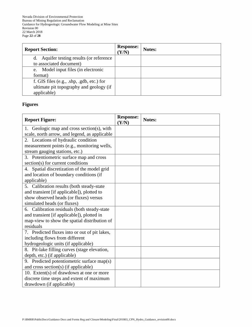
Attachment A: NDEP-BMRR Groundwater Model Review Checklist

This is a list of aspects of hydrogeologic significance that should be reviewed for each groundwater

modeling report. For additional information on any specific aspect mentioned here the reader is referred

to the following documents:

Anderson, M.P., Woessner, W.W., and Hunt, R.J., 2015, Applied groundwater modeling: Simulation of

flow and advective transport, Academic Press, pp. 564.

Barnett, B., Townley, L.R., Post, V., Evans, R.E., Hunt, R.J., Peeters, L., Richardson, S., Werner, A.D.,

Knapton, A., and Boronkay, A., 2012, Australian groundwater modelling guidelines, Waterlines

report series no. 82: National Water Commission, Canberra, pp. 203.

Reilly, T.E. and Harbaugh, A.W., 2004, Guidelines for Evaluating Groundwater Flow Models. United

States Geological Survey Scientific Investigations Report 2004-5038. pp. 29.

Part 1 – Report Information

Project Name:

Permit #:

Model Type: Analytical --- Analytic element --- Numerical (circle one)

Code:

Part 2 – Contents of Report

Text Sections

Report Section: Response:

(Y/N) Notes:

1. Title, project name, permit number,

preparer, and date

2. Executive summary

3. Site background

4. Study objectives and application/need

for groundwater modeling

a. Application of modeling methods

(i.e., analytical versus numerical)

b. Numerical code(s) used, and

reasoning for application (if applicable)




Page 20 of 28



(Y/N) Notes:

i. If the code(s) were modified in

any way for the application at hand,

appropriate material corresponding

to the modification must be

submitted, see specifically Anderson

et al. (2015), Chapter 11.

c. Performance assessment of

previous model iteration (if applicable)

5. Description of groundwater flow system

of interest

a. Geologic framework

b. Hydrologic framework

(groundwater and surface water)

c. Climatologic characteristics

d. Current and past hydraulic

conditions, and geochemical conditions

(if applicable)

6. Description of the conceptual model

and model domain

7. Description of the numerical model (if

applicable)

a. How the conceptual model was

translated to the numerical model,

including spatial and temporal

discretization

8. Description of boundary conditions

9. Description of water budget(s), and

comparison to previously published

estimates (if applicable)

10. Description and evaluation of aquifer

properties and fluxes

a. Sources for aquifer properties and

fluxes included in the model

b. Reasonable ranges for aquifer

properties and fluxes

11. Description of any applied hydraulic

stresses

12. Summary of steady-state calibration

a. Calibration measures




Page 21 of 28



(Y/N) Notes:

b. Interpretation of spatial variability

of calibration residuals and impact on

predictive modeling (if applicable)

13. Summary of transient calibration (if

applicable), to include calibration measures,

as well as other applicable simulations (e.g.,

particle tracking, etc.)

a. Calibration measures

b. Interpretation of spatial and

temporal variability of calibration

residuals and impact on predictive

modeling (if applicable)

14. Summary of history matching (if

applicable )

15. Summary of predictions (if applicable)

16. Summary of sensitivity analyses

a. Quantitative comparisons of results

of the base-case model with sensitivity

analyses, and discussion of how likely

the sensitivity analysis scenario results

are and how these likely scenarios

affect long-term management/outcomes

17. Conclusions of the study

18. Appendices

a. Geographic location and associated

information for all hydraulic condition

measurement points (monitoring wells,

stream gauges, etc.), reported in

accessible numerical format (e.g., CSV,

Excel, etc.) with appropriate metadata

(datum, coordinate system, etc.), or in

geographic information system (GIS)

file formats (e.g., .shp, .gdb, etc.)

b. Geochemical analysis results (if

applicable), reported in accessible

numerical format (e.g., CSV, Excel,

etc.)

c. Calibration hydrographs (both

steady-state and transient [if

applicable])




Page 22 of 28



(Y/N) Notes:

d. Aquifer testing results (or reference

to associated document)

e. Model input files (in electronic

format)

f. GIS files (e.g., .shp, .gdb, etc.) for

ultimate pit topography and geology (if

applicable)

Figures

Report Figure: Response:

(Y/N) Notes:

1. Geologic map and cross section(s), with

scale, north arrow, and legend, as applicable

2. Locations of hydraulic condition

measurement points (e.g., monitoring wells,

stream gauging stations, etc.)

3. Potentiometric surface map and cross

section(s) for current conditions

4. Spatial discretization of the model grid

and location of boundary conditions (if

applicable)

5. Calibration results (both steady-state

and transient [if applicable]), plotted to

show observed heads (or fluxes) versus

simulated heads (or fluxes)

6. Calibration residuals (both steady-state

and transient [if applicable]), plotted in

map-view to show the spatial distribution of

residuals

7. Predicted fluxes into or out of pit lakes,

including flows from different

hydrogeologic units (if applicable)

8. Pit-lake filling curves (stage elevation,

depth, etc.) (if applicable)

9. Predicted potentiometric surface map(s)

and cross section(s) (if applicable)

10. Extent(s) of drawdown at one or more

discrete time steps and extent of maximum

drawdown (if applicable)




Page 23 of 28


Tables

Report Table: Response:

(Y/N) Notes:

1. Climatologic characteristics (e.g., annual

or monthly precipitation and

evaporation)

2. Hydraulic properties of hydrogeologic

units and associated data sources

(aquifer testing, other reports, etc.)

3. Calibration results (both steady-state and

transient [if applicable]), to include all

relevant calibration statistics

4. Groundwater budgets for the model

domain (for any applicable period of the

model simulation), with comparison to

published/targeted quantities (if

applicable)

5. Pit-lake budget(s) including quantities of

inflow and outflow to different

hydrogeologic units (if applicable)

6. Parameter values used in sensitivity

analyses

Part 3 – Model Review

General Considerations

Consideration: Response:

Y / N Notes:

Are the objectives of the study and the level

of confidence clearly stated?

Does the numerical or analytical model

selected for use simulate the important

physical processes needed to adequately

represent the system?

Are the uncertainties associated with the

model clearly stated?

Are all required sections of the report

present (including figures and tables)?




Page 24 of 28


Modeling Approaches


Y / N Notes:

Is the overall approach (calibrated model,

hypothetical system model, sensitivity

analysis, superposition, and particle

tracking) used in addressing the objectives

clearly stated and appropriate?

If the analysis is not three dimensional, is

the representation of the system using one

or two dimensions appropriate to meet the

objectives of the study and justified in the

report?

If the model is steady state, is adequate

information provided to justify that the

system is reasonably close to a steady-state

condition?

Conceptual Model


Y / N Notes:

Is the conceptual model of the system under

investigation reasonable?

Are all physical processes and features

within the model domain incorporated into

the conceptual model?

Is the conceptual model supported by

representative data?

Are there alternate conceptual models that

could be reasonably applied?




Page 25 of 28


Model Discretization and Hydrogeologic Framework


Y / N Notes:

Are all processes included in the conceptual

model also included in the numerical

model?

Does the horizontal discretization represent

the important features of the hydrogeologic

framework to meet the objectives of the

study?

Are the physical boundaries represented

appropriately in space by the discretized

representation?

Is the horizontal discretization appropriate

to represent the degree of complexity in the

aquifer properties and head distribution

(flow system)?

Does the vertical discretization adequately

represent the vertical connectivity and

properties of the hydrogeologic framework

to meet the objectives of the study?

If the groundwater system is unconfined in

some areas, then is the treatment of changes

in saturated thickness and the potential for

cells to go dry explained and appropriate? If

cells have gone dry, does the resultant

solution seem appropriate?

Is the temporal discretization fine enough to

represent the degree of complexity in

stresses and head distribution over time?




Page 26 of 28


Boundary Conditions


Y / N Notes:

Are the mathematical representations of the

boundary conditions reasonable for the

objectives of the study?

Are all the external boundaries of the model

associated with a definable physical

feature?

If no –

a) Is justification provided for the

use of artificial boundaries?

b) Is the justification sufficient?

c) Are the effects of the artificial

boundaries tested in the

calibration of the model and

documented in the report?

d) Does the documentation of

their use and their testing make

a convincing argument for their

reasonableness?

If yes –

a) Is the mathematical

representation of the physical

feature appropriate?

b) Are there conditions under

which the representation of the

boundary used in the model

would become invalid?

c) Are these conditions

discussed?

Do the boundary conditions of the model

overly constrain the model results so that

the calibration is insensitive and the

predictions are not realistic?




Page 27 of 28


Transient Solutions


Y / N Notes:

Does the transient model simulation start

from a steady-state condition?

If yes –

a) Were the initial conditions

generated from a steady-state

simulation of the period of

equilibrium?

b) If the initial conditions were

not generated from a steady-

state simulation of the period

of equilibrium, is there a

compelling reason why they

were not generated, or are the

initial conditions invalid?

If no –

a) Was it possible to select a

period of equilibrium to start

the simulation and make the

determination of initial

conditions more

straightforward? If it is possi-

ble, then the model should

have simulated the transient

period from the period of

equilibrium.

b) If it was not possible to select a

period of equilibrium to start

the simulation, then what was

the justification for selecting

the starting time and the initial

conditions for the simulation?

c) How was it shown that the

initial conditions used did not

bias the result of the

simulation?




Page 28 of 28


Adequacy of Calibration


Y / N Notes:

Does the simulated head and flow

distribution mimic the important aspects of

the flow system, such as magnitude and

direction of the flow vectors?

Does some quantitative measure of head

and flow differences between the simulated

and observed values seem reasonable for the

objectives of the investigation?

Does the distribution of areas where

simulated heads are too high and areas

where simulated heads are too low seem

randomly distributed? If they are not

randomly distributed, then is there a

hydrogeologic justification to change the

model and make the residuals more random

aerially?

Has a short-term performance assessment

been completed (e.g., a history match), and

if so are the results acceptable?

Uncertainty and Sensitivity Analysis


Y / N Notes:

Has the sensitivity analysis included

reasonable parameters and parameter values

to encompass possible conditions on the

site?

Are the sources of uncertainty discussed?

Has some quantitative or qualitative

assessment of uncertainty been made?

Have suggestions to reduce uncertainty in

future models (e.g., data gathering,

additional testing, etc.) been included?

Nevada Division of Environmental Protection Bureau of … for Hydrogeologic Groundwater Flow Modeling at Mine Sites Prepared by Connor P. Newman 22 March 2018 1. Introduction Mining

Documents