NEUTRINO OSCILLATIONS IN PARTICLE PHYSICS AND ASTROPHYSICS Memoria de Tesis Doctoral realizada por Iv´ an Jes´ us Mart´ ınez Soler presentada ante el Departamento de F´ ısica Te´ orica de la Universidad Aut´ onoma de Madrid para optar al t´ ıtulo de Doctor en F´ ısica Te´ orica. Tesis dirigida por el Prf. D. Michele Maltoni Cient´ ıfico titular del Instituto de F´ ısica Te´ orica UAM-CSIC Departamento de F´ ısicaTe´orica Universidad Aut´ onoma de Madrid Instituto de F´ ısica Te´ orica UAM-CSIC Mayo de 2018

Welcome message from author
This document is posted to help you gain knowledge. Please leave a comment to let me know what you think about it! Share it to your friends and learn new things together.
Transcript
NEUTRINO OSCILLATIONS INPARTICLE PHYSICS AND
ASTROPHYSICS
Memoria de Tesis Doctoral realizada por
Ivan Jesus Martınez Soler
presentada ante el Departamento de Fısica Teoricade la Universidad Autonoma de Madrid
para optar al tıtulo de Doctor en Fısica Teorica.
Tesis dirigida por el Prf. D. Michele MaltoniCientıfico titular del Instituto de Fısica Teorica UAM-CSIC
Departamento de Fısica Teorica
Universidad Autonoma de Madrid
Instituto de Fısica Teorica UAM-CSIC
Mayo de 2018
Agradecimientos
Para mı, una tesis doctoral no consiste solamente en los resultados que a contin-uacion se presentan, sino que es un largo e intenso proceso de aprendizaje, en el queun joven estudiante es guiado por su maestro, a traves de la consecucion de unaspequenas metas, en el descubrimiento de un vasto universo de conocimiento. Comoya he dicho, este camino no se recorre solo, y para mi fortuna he tenido al mejorguıa que podıa tener, el Prof. Michele Maltoni. Sin sus ensenanzas, consejos, ayudae infinita paciencia, recorrer el largo trayecto que me ha traido hasta aquı hubierasido imposible. Por ello, nada mas me gustarıa en este momento, que agradecerletodos estos anos de maxima felicidad en los que ha llegado a ser mas que un profesorpara mı.
A lo largo de este tiempo he tenido la gran oportunidad de aprender trabajandojunto a fısicos increıbles, quienes, ademas de hacer posible todo lo que aquı serecoge, me han ayudado a comprender mejor el mundo de la fısica. Solo puedo estarenormemente agradecido a Concha Gonzalez-Garcıa y Pilar Coloma por su acogida,dedicacion y esfuerzo conmigo, remarco esto ultimo, y porque me han ensenado queincluso a una distancia de miles de kilometros y varias horas de diferencia, uno puedesentirse como en casa.
Querrıa tambien agradecer a todos aquellos con quienes he tenido la oportunidadde colaborar en diferentes proyectos. A Jacobo Lopez-Pavon, Pedro A.N. Machado,Ivan Esteban, Hiroshi Nunokawa, Hisakazu Minakata y Ninqiang Song. Una granparte de este trabajo tambien es gracias a ellos.
A mis padres, hermanos y abuela, por su constante apoyo y motivacion. Quieneshan hecho lo imposible para que yo pudiera sonar con este momento. A mis padrinosy a Juan Jesus, por confiar en mı y alentarme en todo este tiempo.
A mis amigos cientıficos. Por los eternos momentos vividos en cenas, en in-terminables viajes a Murcia o en infinitas partidas a juegos de mesa. Por las in-terminables charlas, algunas incluso sobre fısica, que me han supuesto una fuenteinagotable de sabidurıa. Me gustarıa en especial mencionar a Pedro Fernandez-Ramirez, Nieves Lopez, Pablo Cano, Loles, Alejandro Ruiperez, Oscar Lasso, Mar-garita, Jose Angel Romero, Eduardo Ibanez, Manuel Trashorras, Pablo Bueno y AnaCueto. Y a mis amigos de toda la vida, por todas las “constructivas” discusionesmantenidas.
Y sobre todo a Veronica. Porque a lo largo de una tesis no todos los momentosson buenos ni sencillos, pero ella siempre ha estado a mi lado, sea cual sea la distanciaque nos separe, compartiendo todas mis alegrıas y haciendo mucho mas llevaderoslos malos momentos. Porque siempre me ha apoyado en todas las decisiones, pormuy difıciles que sean de entender. Porque sin ella no me habrıa atrevido a darmuchos de los pasos que he dado, ni a comenzar esta aventura. Porque siempre meha aconsejado seguir y nunca rendirme. En definitiva, por todo.
3

Abstract
Neutrinos are described in the Standard Model (SM) by three left-handed fermionfields, one for each fermion generation. In the SM, the masses of the fermions arisesas a Yukawa interaction between the right-handed and the left-handed fermion fields,and the Higgs doublet. Because of the lack of a right-handed field for neutrinos,these fermions are massless within the SM. Experiments measuring the flavor com-position of neutrinos have stablished the oscillation of the flavor along its path. Thisoscillation can be explained in the scenario of a mixing between neutrino flavor andneutrino mass states. This thesis is devoted to the study of the neutrino flavor oscil-lations within different mixing models. In particular, it is focused into the physicsreach by the new generation of neutrino telescopes, like IceCube and DeepCore.
The low energy part of the atmospheric neutrino flux measured by DeepCorelead a sizable flavor oscillation in the muon disappearance channel (νµ → νµ). Bycombining the latest experimental data collected by this detector (up to 2016) withthe results of other oscillation experiments, we have performed a global fits withinthe three-neutrino mixing framework. In this work has been also discussed thecomplementarity role played by atmospheric/accelerator and the reactor data onthe determination of the atmospheric mass parameter.
IceCube can be also considered as a tool to look for New Physics signals. Theminimal extension of the SM to explain the neutrino masses consist of a heavyright-handed neutrino field. The mass of this new fermion is not predicted by anymodel, it can take any value over a wide range of orders of magnitude. For massesaround GeV, we have studied in a different work the detection of the new fermion bylooking for “Double-Cascades” events topologies. We have considered two differentscenarios where the signal can be created by a heavy neutrino, the mixing of theheavy state with a light neutrino through a NC, and the production of the heavystate via a transition magnetic moment. The results indicate that IceCube improvethe current bounds in the scenarios considered for heavy states with masses around1 GeV.
Another New Physics scenario considered is the so-called Quantum Decoherence,which introduces a damping effect on the flavor oscillation. In a recent work, wehave developed a new formalism to study this effect through non-adiabatic matter.By a fit of the atmospheric events measured by IceCube and DeepCore, it is shownthat these experiments improve over the current bound from other experiments.
The primary goal of IceCube is the detection of astrophysical neutrinos, whathappened in 2013. This energetic events opens the possibility to study New Physicson them. In another, work we have considered the impact of Non-Standard Inter-actions on the flavor of this events, finding large deviations from the three-neutrinomixing prediction.
Neutrino physics is moving into the precission era, but still a lot of fundamentaland exciting problems remain without answer. This converts to this reach area in avery promising field for the near future.
5
Resumen
Los neutrinos estan descritos en el Modelo Estandar (MS) por tres camposfermionicos zurdos, uno por cada generacion de fermiones. En el MS, el terminode masa para cada fermion cargado viene dado por una interaccion de Yukawa entrelos campos zurdos y diestros de dicho fermion, con el campo de Higgs. Debido a queen el SM no hay campo diestro para los neutrinos, estas partıculas no poseen masa.Los experimentos que han medido el sabor de los neutrinos han establecido que elsabor de estas partıculas oscila a lo largo de su trayectoria. Esta oscilacion puedeser explicada por acoplo entre estados de sabor y estados de masa. Esta tesis secentra en el estudio de las oscilaciones de neutrinos para diferentes modelos teoricosque describen este acoplo. En particular, se ha enfocado al estudio de la fısica quepuede ser medida en la nueva generacion de telescopios de neutrinos, como IceCubey DeepCore.
La parte de baja energıa del espectro de neutrinos atmospfericos medido porDeepCore permite observar las oscilaciones de neutrinos en el canal (νµ → νµ). Com-binando los ultimos resultados experimentales recogidos por este experimento (hasta2016), junto con los resultados del resto de experimentos de oscilaciones de neutri-nos, hemos realizado un ajuste global de los parametros de oscilacion en el modelode mezcla de tres neutrinos. En este trabajo tambien ha sido discutida la comple-mentariedad entre las medidas de experimentos atmosfericos/aceleradores con lasmedidas en reactores en la determinacion del parametro de masas atmosferico.
IceCube tambien puede ser usado en la busqueda de senales de nueva fısica. Lamınima extension del MS necesaria para explicar la masa de los neutrinos consisteen anadir campos diestros para los neutrinos. La masa de estos nuevos fermionesno esta fijada por ningun modelo. Hemos estudiado la deteccion de estos nuevosfermiones con masas entorno al GeV buscando eventos con la topologıa “Double-Cascade”. Para ello, hemos considerado dos escenarios diferentes donde esta senalpuede ser creada por la nueva partıcula, un acoplo entre los campos diestros y losneutrinos descritos en el MS, y un momento magnetico de transicion.
Otro escenario de nueva fısica considerado, en este caso en neutrinos atmosfericos,es el denominado como Decoherencia Quantica, el cual introduce una amortiguacionen la oscilacion de sabor. A traves de un ajuste de los eventos atmosfericos medidospor IceCube y DeepCore, se ha observado una mejora en la precision con que losefectos de este modelo de nueva fısica pueden ser medidos.
El objetivo principal de IceCube es la deteccion de neutrinos astrofısicos, que tuvolugar en 2013. La observacion de estos eventos energeticos ha abierto la posibilidadde buscar en ellos procesos de nueva fısica. Por ello, en otro trabajo hemos estudiadoel impacto que puede tener la existencia de nuevas interacciones en el sabor de estoseventos. Los resultados muestran grandes desviaciones con respecto a lo predichopor el modelo de tres neutrinos.
La fısica de neutrinos se esta encaminando hacia una era de precision, perotodavıa existen problemas excitantes y fundamentales sin resolver. Esto convierte aeste area de investigacion en un campo muy prometedor para el futuro.
7

Contents
Abstract 5
Resumen 7
1 Introduction 111.1 Historical introduction . . . . . . . . . . . . . . . . . . . . . . . . . . 111.2 Neutrinos in the SM . . . . . . . . . . . . . . . . . . . . . . . . . . . 12
1.2.1 Electroweak interaction . . . . . . . . . . . . . . . . . . . . . . 131.2.2 Higgs mechanism . . . . . . . . . . . . . . . . . . . . . . . . . 14
1.3 Neutrino masses . . . . . . . . . . . . . . . . . . . . . . . . . . . . . . 161.3.1 The see-saw mechanism . . . . . . . . . . . . . . . . . . . . . 171.3.2 Leptonic Mixing . . . . . . . . . . . . . . . . . . . . . . . . . . 17
1.4 Neutrino flavor oscillations . . . . . . . . . . . . . . . . . . . . . . . . 181.4.1 Vacuum neutrino oscillations . . . . . . . . . . . . . . . . . . . 191.4.2 CPT, CP and T transformations . . . . . . . . . . . . . . . . 211.4.3 2ν approximation . . . . . . . . . . . . . . . . . . . . . . . . . 211.4.4 Mass splitting dominance . . . . . . . . . . . . . . . . . . . . 22
1.5 Neutrino oscillation in matter . . . . . . . . . . . . . . . . . . . . . . 231.5.1 Neutrino coherent interaction . . . . . . . . . . . . . . . . . . 241.5.2 Flavor oscillation in constant matter . . . . . . . . . . . . . . 261.5.3 2ν approximation . . . . . . . . . . . . . . . . . . . . . . . . . 271.5.4 Adiabatic approximation . . . . . . . . . . . . . . . . . . . . . 28
1.6 Atmospheric neutrinos . . . . . . . . . . . . . . . . . . . . . . . . . . 291.6.1 Atmospheric neutrino flux calculations . . . . . . . . . . . . . 301.6.2 Flavor oscillation in the Earth . . . . . . . . . . . . . . . . . . 311.6.3 IceCube DeepCore experiment . . . . . . . . . . . . . . . . . . 34
2 Fit to three neutrino mixing 39
3 Double-Cascades Events from New Physics in IceCube 71
4 NSI and astrophysical neutrinos 77
5 Decoherence in neutrino propagation through matter 87
6 Conclusions 121
Conclusiones 125
Bibliography 129
9

Chapter1
Introduction
1.1 Historical introduction
The first evidence of neutrino oscillation was observed in the Kamiokande ex-periment, a detector that which built to discover the proton decay, predicted bythe Electroweak Theory. Kamiokande was a water Cherenkov detector located ata depth of 1 km in Kamioka (Japan), which started to take data in 1983 [1]. Thecharged particles created in the proton decay propagate at relativistic speeds onwater, and emit Cherenkov radiation that is detected by the photomultiplier sur-rounding the water tank. The dominant background was the atmospheric neutrinointeractions that were produced by charged leptons.
The interaction of cosmic rays with the atmospheric nuclei produces π and K,that decay mainly in µ and νµ. A second particle generation is created after µdecay into νµ, e and νe. So, νµ and νe are mainly produced in the atmosphere in aflavor ratio 2:1 (νµ : νe). In 1988, Kamiokande showed a deficit in the number of νµcompared with the simulation results, that could not be explained by the systematicsdetector effects or by the uncertainties in the atmospheric flux prediction [2]. Dueto the low precision in the flux calculation, the results were presented in terms of theflavor ratio νµ over νe. This flavor ratio is theoretically predicted to be around 2, andup-down symmetric for higher energies (multi-GeV). For lower energies (sub-GeV),the magnetic field of the Earth modifies the cosmic ray flux. The results showedthe 59 ± 7% of the expected number for νµ [2]. The deficit was also confirmed byanother water Cherenkov experiment, IMB [3].
In 1996, a new detector was built with a fiducial volume twenty times larger thanKamiokande volume, what made possible enlarge the statistics by the same factor.The number of photomultipliers used in the new experiment was larger comparedwith Kamiokande, what allowed the measurement of the neutrino interaction withhigher precision. The new experiment was called Super-Kamiokande. In 1998,after two years of data taking, the experiment announced evidence for atmosphericneutrino oscillations with a significance of 6σ [1, 4, 5], Fig 1.1. The results showeda deficit in the up-going νµ flux that depended on the zenith angle. For the down-going neutrinos, the prediction agrees with the data. For the νe events was observedno deviation from the prediction. A combined analysis of the Kamiokande andSuper-Kamiokande measurement showed that neutrino oscillation could consistentlyexplain both results. The results were confirmed by MACRO [6] and Soundan-2 [7],two experiments which also observed a zenith-angle dependence deficit in νµ.
11

1.2 Neutrinos in the SM
1.2 Neutrinos in the SM
The Standard Model (SM) describe the interactions between three generationsof fermions, versus gauge bosons and one scalar, the Higgs boson, according to thegauge group
SU(3)C × SU(2)L × U(1)Y (1.1)
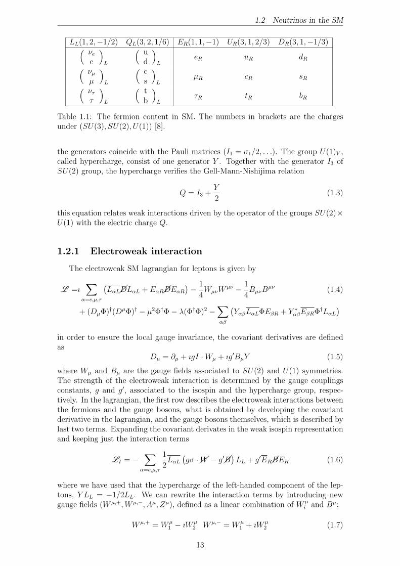
Each generation consists of five fermions (Table 1.1), with a different represen-tation under the symmetry group each of them [8]. The fermions have the samecharges under the symmetry group in the three generations, but they present dif-ferent masses. The SM gauge group together with the fermion content present anaccidental global symmetry
U(1)B × U(1)Le × U(1)Lµ × U(1)Lτ (1.2)
that preserve the baryon number (B) and the three lepton numbers (Le, Lµ, Lτ ),and as a result, the total lepton number L = Le + Lµ + Lτ . That global symmetryis a consequence of the SM gauge symmetry and the representation of the physicalstates.
The subgroup SU(2) × U(1), called electroweak symmetry group, unifies theelectromagnetism and the weak theory and is the only group that acts non-triviallyover the neutrino field. These fermions are not affected by strong or electromagneticinteractions, so they are singlets of SU(3)c×U(1)Q. The group SU(2), called isospin,acts over the left-handed chiral component of the fermions field, whereas the right-handed components are singlets. It has three generators Ia(a = 1, 2, 3) that verifiesthe commutation relations [Ia, Ib] = ıεabcIc. In a two dimensional representation,
Figure 1.1: Zenith angle distribution events presented by Super-Kamiokande collab-oration at the Neutrino ’98 [1, 4, 5]
12
1.2 Neutrinos in the SM
LL(1, 2,−1/2) QL(3, 2, 1/6) ER(1, 1,−1) UR(3, 1, 2/3) DR(3, 1,−1/3)( νee
)L
( ud
)L
eR uR dR( νµ
µ
)L
( cs
)L
µR cR sR( ντ
τ
)L
( tb
)L
τR tR bR
Table 1.1: The fermion content in SM. The numbers in brackets are the chargesunder (SU(3), SU(2), U(1)) [8].
the generators coincide with the Pauli matrices (I1 = σ1/2, . . .). The group U(1)Y ,called hypercharge, consist of one generator Y . Together with the generator I3 ofSU(2) group, the hypercharge verifies the Gell-Mann-Nishijima relation
Q = I3 +Y
2(1.3)
this equation relates weak interactions driven by the operator of the groups SU(2)×U(1) with the electric charge Q.
1.2.1 Electroweak interaction
The electroweak SM lagrangian for leptons is given by
L =ı∑
α=e,µ,τ
(LαL��DLαL + EαR��DEαR
)− 1
4WµνW
µν − 1
4BµνB
µν (1.4)
+ (DµΦ)†(DµΦ)† − µ2Φ†Φ− λ(Φ†Φ)2 −∑
αβ
(YαβLαLΦEβR + Y ∗αβEβRΦ†LαL
)
in order to ensure the local gauge invariance, the covariant derivatives are definedas
Dµ = ∂µ + ıgI ·Wµ + ıg′BµY (1.5)
where Wµ and Bµ are the gauge fields associated to SU(2) and U(1) symmetries.The strength of the electroweak interaction is determined by the gauge couplingsconstants, g and g′, associated to the isospin and the hypercharge group, respec-tively. In the lagrangian, the first row describes the electroweak interactions betweenthe fermions and the gauge bosons, what is obtained by developing the covariantderivative in the lagrangian, and the gauge bosons themselves, which is described bylast two terms. Expanding the covariant derivates in the weak isospin representationand keeping just the interaction terms
LI = −∑
α=e,µ,τ
1
2LαL
(gσ ·��W − g′��B
)LL + g′ER��BER (1.6)
where we have used that the hypercharge of the left-handed component of the lep-tons, Y LL = −1/2LL. We can rewrite the interaction terms by introducing newgauge fields (W µ,+,W µ,−, Aµ, Zµ), defined as a linear combination of W µ
i and Bµ:
W µ,+ = W µ1 − ıW µ
2 W µ,− = W µ1 + ıW µ
2 (1.7)
13
1.2 Neutrinos in the SM
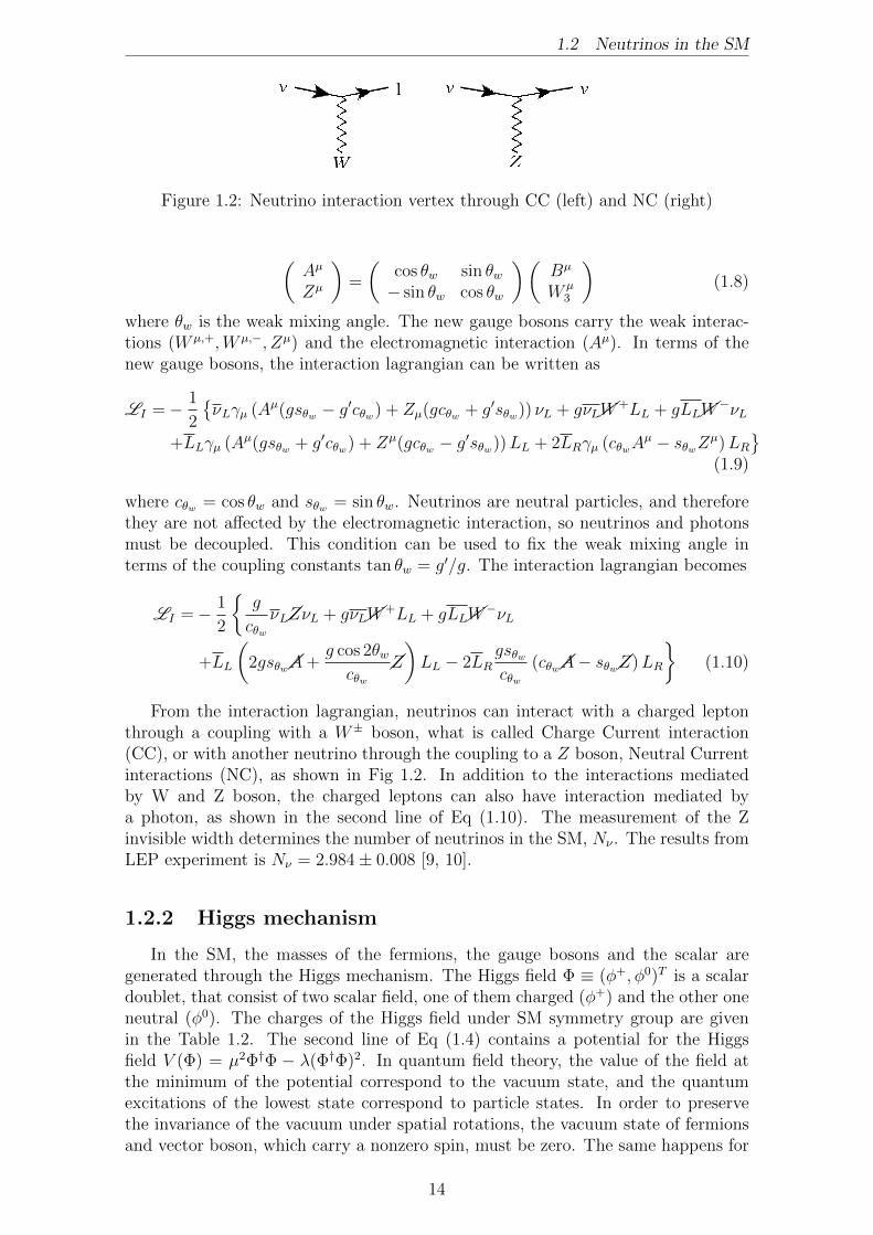
Figure 1.2: Neutrino interaction vertex through CC (left) and NC (right)
(Aµ
Zµ
)=
(cos θw sin θw− sin θw cos θw
)(Bµ
W µ3
)(1.8)
where θw is the weak mixing angle. The new gauge bosons carry the weak interac-tions (W µ,+,W µ,−, Zµ) and the electromagnetic interaction (Aµ). In terms of thenew gauge bosons, the interaction lagrangian can be written as
LI =− 1
2
{νLγµ (Aµ(gsθw − g′cθw) + Zµ(gcθw + g′sθw)) νL + gνL��W
+LL + gLL��W−νL
+LLγµ (Aµ(gsθw + g′cθw) + Zµ(gcθw − g′sθw))LL + 2LRγµ (cθwAµ − sθwZµ)LR
}
(1.9)
where cθw = cos θw and sθw = sin θw. Neutrinos are neutral particles, and thereforethey are not affected by the electromagnetic interaction, so neutrinos and photonsmust be decoupled. This condition can be used to fix the weak mixing angle interms of the coupling constants tan θw = g′/g. The interaction lagrangian becomes
LI =− 1
2
{g
cθwνL��ZνL + gνL��W
+LL + gLL��W−νL
+LL
(2gsθw��A+
g cos 2θwcθw
��Z
)LL − 2LR
gsθwcθw
(cθw��A− sθw��Z)LR
}(1.10)
From the interaction lagrangian, neutrinos can interact with a charged leptonthrough a coupling with a W± boson, what is called Charge Current interaction(CC), or with another neutrino through the coupling to a Z boson, Neutral Currentinteractions (NC), as shown in Fig 1.2. In addition to the interactions mediatedby W and Z boson, the charged leptons can also have interaction mediated bya photon, as shown in the second line of Eq (1.10). The measurement of the Zinvisible width determines the number of neutrinos in the SM, Nν . The results fromLEP experiment is Nν = 2.984± 0.008 [9, 10].
1.2.2 Higgs mechanism
In the SM, the masses of the fermions, the gauge bosons and the scalar aregenerated through the Higgs mechanism. The Higgs field Φ ≡ (φ+, φ0)T is a scalardoublet, that consist of two scalar field, one of them charged (φ+) and the other oneneutral (φ0). The charges of the Higgs field under SM symmetry group are givenin the Table 1.2. The second line of Eq (1.4) contains a potential for the Higgsfield V (Φ) = µ2Φ†Φ − λ(Φ†Φ)2. In quantum field theory, the value of the field atthe minimum of the potential correspond to the vacuum state, and the quantumexcitations of the lowest state correspond to particle states. In order to preservethe invariance of the vacuum under spatial rotations, the vacuum state of fermionsand vector boson, which carry a nonzero spin, must be zero. The same happens for
14
1.2 Neutrinos in the SM
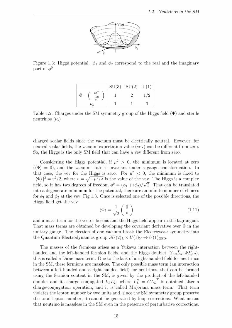
Figure 1.3: Higgs potential. φ1 and φ2 correspond to the real and the imaginarypart of φ0
SU(3) SU(2) U(1)
Φ =( φ+
φ0
)1 2 1/2
νs 1 1 0
Table 1.2: Charges under the SM symmetry group of the Higgs field (Φ) and sterileneutrinos (νs)
charged scalar fields since the vacuum must be electrically neutral. However, forneutral scalar fields, the vacuum expectation value (vev) can be different from zero.So, the Higgs is the only SM field that can have a vev different from zero.
Considering the Higgs potential, if µ2 > 0, the minimum is located at zero(〈Φ〉 = 0), and the vacuum state is invariant under a gauge transformation. Inthat case, the vev for the Higgs is zero. For µ2 < 0, the minimum is fixed to| 〈Φ〉 |2 = v2/2, where v =
√−µ2/λ is the value of the vev. The Higgs is a complex
field, so it has two degrees of freedom φ0 = (φ1 + ıφ2)/√
2. That can be translatedinto a degenerate minimum for the potential, there are an infinite number of choicesfor φ1 and φ2 at the vev, Fig 1.3. Once is selected one of the possible directions, theHiggs field get the vev
〈Φ〉 =1√2
(0v
)(1.11)
and a mass term for the vector bosons and the Higgs field appear in the lagrangian.That mass terms are obtained by developing the covariant derivative over Φ in theunitary gauge. The election of one vacuum break the Electroweak symmetry intothe Quantum Electrodynamics group SU(2)L × U(1)Y → U(1)QED.
The masses of the fermions arises as a Yukawa interaction between the right-handed and the left-handed fermion fields, and the Higgs doublet (YαβLαLΦEβR),this is called a Dirac mass term. Due to the lack of a right-handed field for neutrinosin the SM, these fermions are massless. The only possible mass term (an interactionbetween a left-handed and a right-handed field) for neutrinos, that can be formedusing the fermion content in the SM, is given by the product of the left-handed
doublet and its charge conjugated LLLcL, where LCL = CLL
Tis obtained after a
charge-conjugation operation, and it is called Majorana mass term. That termviolates the lepton number by two units and, since the SM symmetry group preservethe total lepton number, it cannot be generated by loop corrections. What meansthat neutrino is massless in the SM even in the presence of perturbative corrections.
15
1.2 Neutrinos in the SM
1.3 Neutrino masses
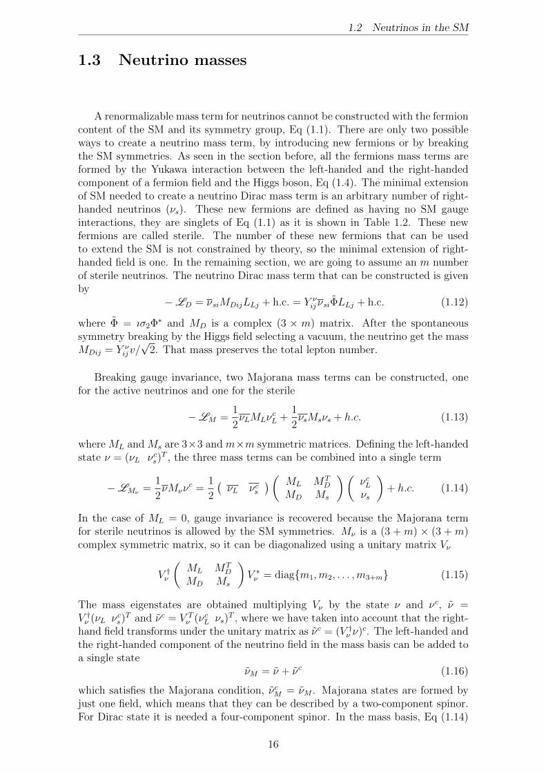
A renormalizable mass term for neutrinos cannot be constructed with the fermioncontent of the SM and its symmetry group, Eq (1.1). There are only two possibleways to create a neutrino mass term, by introducing new fermions or by breakingthe SM symmetries. As seen in the section before, all the fermions mass terms areformed by the Yukawa interaction between the left-handed and the right-handedcomponent of a fermion field and the Higgs boson, Eq (1.4). The minimal extensionof SM needed to create a neutrino Dirac mass term is an arbitrary number of right-handed neutrinos (νs). These new fermions are defined as having no SM gaugeinteractions, they are singlets of Eq (1.1) as it is shown in Table 1.2. These newfermions are called sterile. The number of these new fermions that can be usedto extend the SM is not constrained by theory, so the minimal extension of right-handed field is one. In the remaining section, we are going to assume an m numberof sterile neutrinos. The neutrino Dirac mass term that can be constructed is givenby
−LD = νsiMDijLLj + h.c. = Y νijνsiΦLLj + h.c. (1.12)
where Φ = ıσ2Φ∗ and MD is a complex (3 × m) matrix. After the spontaneoussymmetry breaking by the Higgs field selecting a vacuum, the neutrino get the massMDij = Y ν
ijv/√
2. That mass preserves the total lepton number.
Breaking gauge invariance, two Majorana mass terms can be constructed, onefor the active neutrinos and one for the sterile
−LM =1
2νLMLν
cL +
1
2νsMsνs + h.c. (1.13)
where ML and Ms are 3×3 and m×m symmetric matrices. Defining the left-handedstate ν = (νL νcs)
T , the three mass terms can be combined into a single term
−LMν =1
2νMνν
c =1
2
(νL νcs
)( ML MTD
MD Ms
)(νcLνs
)+ h.c. (1.14)
In the case of ML = 0, gauge invariance is recovered because the Majorana termfor sterile neutrinos is allowed by the SM symmetries. Mν is a (3 + m) × (3 + m)complex symmetric matrix, so it can be diagonalized using a unitary matrix Vν
V †ν
(ML MT
D
MD Ms
)V ∗ν = diag{m1,m2, . . . ,m3+m} (1.15)
The mass eigenstates are obtained multiplying Vν by the state ν and νc, ν =V †ν (νL νcs)
T and νc = V Tν (νcL νs)
T , where we have taken into account that the right-hand field transforms under the unitary matrix as νc = (V †ν ν)c. The left-handed andthe right-handed component of the neutrino field in the mass basis can be added toa single state
νM = ν + νc (1.16)
which satisfies the Majorana condition, νcM = νM . Majorana states are formed byjust one field, which means that they can be described by a two-component spinor.For Dirac state it is needed a four-component spinor. In the mass basis, Eq (1.14)
16

1.3. NEUTRINO MASSES
can be rewriten as
−LMν =1
2
3+m∑
k=1
mkνM,kνM,k =1
2
3+m∑
k=1
mk(νkνck + ν
c
kνk) (1.17)
where we have used νcνc = −νν. So, the most general mass term that can beconstructed for neutrinos can be written as a Majorana mass term. Unless V =I(3+m)×(3+m), which is equivalent to a diagonal mass matrix in the interaction basis,the flavor states, identified by the fields in the interaction lagrangian, and the massstates are not identical. That mismatch implies a flavor lepton mixing.
1.3.1 The see-saw mechanism
The scale of MD should be of the order of the electroweak symmetry breaking(MD ∼ 174 GeV). Since ML break gauge invariance in the neutrino mass matrix,we consider it zero (ML = 0). For the third mass matrix, we can expect Ms >> MD
since it is generated by physics beyond the SM. Considering the strong hierarchybetween the scales of the mass matrices, Mν can be diagonalized by blocks up tocorrections of the order of o(MD/Ms)
V †νMνVν =
(Mlight 0
0 Mheavy
)(1.18)
whereMlight ' −MT
DM−1s MD Mheavy 'Ms (1.19)
and
Vν '(
1− 12M †
D(M∗s )−1M−1
s MD M †D(M∗
s )−1
−(Ms)−1MD 1− 1
2(Ms)
−1MDM†D(M∗
s )−1
)(1.20)
The eigenvalues are in two different scales. The scale of heavier states is of the orderof Ms, whereas for the lightest states its mass is suppressed by MT
DM−1s . This is
called the see-saw mechanism, which can explain the small values of active neutrinomasses just in term of a very heavy sterile neutrino and avoiding very small Yukawacouplings.
1.3.2 Leptonic Mixing
In general, the representation of a field in the interaction basis can be differentfrom the representation in the mass basis. In the SM, neutrinos are massless. Sincethe flavor is defined in the interaction basis, and because the neutrino flavor coin-cides with the charged lepton flavor, the interaction basis for neutrinos and chargedleptons coincides. Without loss of generality, we can choose the basis where massand the interaction states for the charged leptons coincide. If the SM is extendedby a neutrino mass term, the mass basis for neutrinos and charged leptons do nothave to coincide, and this mismatch can lead to a flavor lepton mixing. In orderto see clearly where the mixing is coming from, in the following we are going toassume that the flavor and the mass basis for the charged leptons do not coincide.Let consider the mass term for the charged leptons and the neutrinos written in the
17

1.2 Neutrinos in the SM
interaction basis
−Llepton = LLMLER +1
2νMνν
c (1.21)
we can define two 3 × 3 unitary matrices VL and VR, which diagonalize the massmatrix for the charged leptons V †LMLVR = diag(me,mµ,mτ ). Using Vν to diagonalizeMν as in Eq (1.15), the mass terms for charged leptons and neutrinos can be writtenin the mass basis as
−Llepton = LLdiag(me,mµ,mτ )ER +1
2νdiag(m1, . . . ,m3+m)νc (1.22)
where LL = V †LLL and ER = VRER. Using VL and Vν , the CC interaction Eq (1.10)can be written in the mass basis
LCC = −g2
∑
α
LαLγµναLWµ,− + h.c. (1.23)
= −g2
∑
α
∑
ij
LiLγµVαi,LV′†αj,ν νjLW
µ,− + h.c.
where V ′†ν is a 3× (3 +m) complex matrix that relates the left-handed flavor states(νeL, νµL, ντL) with the mass states (ν1, . . . , ν3+m), and verifies
V ′†ν V′ν = I3×3 V ′νV
′†ν 6= I(3+m)×(3+m) (1.24)
U = VLV′†ν is the mixing matrix in the leptonic sector. The number of inde-
pendent parameters depends on the nature of neutrinos. For pure Majorana states,U can be parametrize with 3(m + 1) angles and 3(m + 1) complex phases. ForDirac neutrinos, U contains 3(m + 1) angles and (2m + 1) phases. There are twoparticular cases where U is a unitary matrix, for 3 Majorana neutrinos without anyadditional sterile neutrino, and for 3 Dirac neutrinos. For 3 Majorana neutrinos,U is parametrized by 3 angles and 3 complex phases, U is conventionally writtenas [10]
U =
1 0 00 c23 s23
0 −s23 c23
c13 0 s13e−ıδcp
0 1 0−s13e
−ıδcp 0 c13
c12 s12 0−s12 c12 0
0 0 1
1 0 0
0 eıδM1 0
0 0 eıδM2
(1.25)For 3 Dirac neutrinos, the phases δM1 and δM2 are absorbed in the neutrino states.
1.4 Neutrino flavor oscillations
Neutrino experiments have established the oscillation of the flavor on the neu-trino path. The experiments have also measured the wavelength showing a de-pendence on the distance traveled and the neutrino energy. Most of the signalsmeasured by experiments can be explained in the framework of the three neutrinomixing. In this model, there are three massive neutrinos that can be expressed asa quantum superposition of the flavor states in the SM (Table 1.1) weighted by thelepton mixing matrix
να =∑
i
Uαiνi (1.26)
18
1.4. NEUTRINO FLAVOR OSCILLATIONS
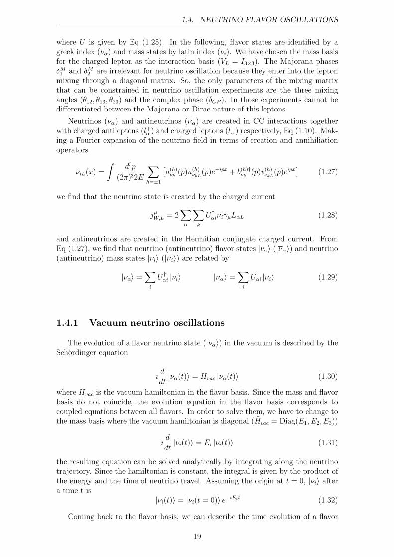
where U is given by Eq (1.25). In the following, flavor states are identified by agreek index (να) and mass states by latin index (νi). We have chosen the mass basisfor the charged lepton as the interaction basis (VL = I3×3). The Majorana phasesδM1 and δM2 are irrelevant for neutrino oscillation because they enter into the leptonmixing through a diagonal matrix. So, the only parameters of the mixing matrixthat can be constrained in neutrino oscillation experiments are the three mixingangles (θ12, θ13, θ23) and the complex phase (δCP ). In those experiments cannot bedifferentiated between the Majorana or Dirac nature of this leptons.
Neutrinos (να) and antineutrinos (να) are created in CC interactions togetherwith charged antileptons (l+α ) and charged leptons (l−α ) respectively, Eq (1.10). Mak-ing a Fourier expansion of the neutrino field in terms of creation and annihiliationoperators
νiL(x) =
∫d3p
(2π)32E
∑
h=±1
[a(h)νk
(p)u(h)νkL
(p)e−ıpx + b(h)†νk
(p)v(h)νkL
(p)eıpx]
(1.27)
we find that the neutrino state is created by the charged current
jµW,L = 2∑
α
∑
k
U †αiνiγµLαL (1.28)
and antineutrinos are created in the Hermitian conjugate charged current. FromEq (1.27), we find that neutrino (antineutrino) flavor states |να〉 (|να〉) and neutrino(antineutrino) mass states |νi〉 (|νi〉) are related by
|να〉 =∑
i
U †αi |νi〉 |να〉 =∑
i
Uαi |νi〉 (1.29)
1.4.1 Vacuum neutrino oscillations
The evolution of a flavor neutrino state (|να〉) in the vacuum is described by theSchordinger equation
ıd
dt|να(t)〉 = Hvac |να(t)〉 (1.30)
where Hvac is the vacuum hamiltonian in the flavor basis. Since the mass and flavorbasis do not coincide, the evolution equation in the flavor basis corresponds tocoupled equations between all flavors. In order to solve them, we have to change tothe mass basis where the vacuum hamiltonian is diagonal (Hvac = Diag(E1, E2, E3))
ıd
dt|νi(t)〉 = Ei |νi(t)〉 (1.31)
the resulting equation can be solved analytically by integrating along the neutrinotrajectory. Since the hamiltonian is constant, the integral is given by the product ofthe energy and the time of neutrino travel. Assuming the origin at t = 0, |νi〉 aftera time t is
|νi(t)〉 = |νi(t = 0)〉 e−ıEit (1.32)
Coming back to the flavor basis, we can describe the time evolution of a flavor
19
1.2 Neutrinos in the SM
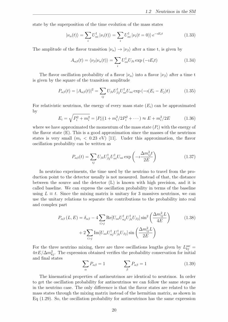
state by the superposition of the time evolution of the mass states
|να(t)〉 =∑
i
U †αi |νi(t)〉 =∑
i
U †αi |νi(t = 0)〉 e−ıEit (1.33)
The amplitude of the flavor transition |να〉 → |νβ〉 after a time t, is given by
Aαβ(t) = 〈νβ|να(t)〉 =∑
i
U †αiUβi exp (−ıEit) (1.34)
The flavor oscillation probability of a flavor |να〉 into a flavor |νβ〉 after a time tis given by the square of the transition amplitude
Pαβ(t) = |Aαβ(t)|2 =∑
ij
UβiU†βjU
†αiUαi exp (−ı(Ei − Ej)t) (1.35)
For relativistic neutrinos, the energy of every mass state (Ei) can be approximatedby
Ei =√P 2i +m2
i = |Pi|(1 +m2i /2P
2i + · · · ) ≈ E +m2
i /2E (1.36)
where we have approximated the momentum of the mass state (Pi) with the energy ofthe flavor state (E). This is a good approximation since the masses of the neutrinosstates is very small (mi < 0.23 eV) [11]. Under this approximation, the flavoroscillation probability can be written as
Pαβ(t) =∑
ij
UβiU†βjU
†αiUαi exp
(−ı∆m
2ijt
2E
)(1.37)
In neutrino experiments, the time used by the neutrino to travel from the pro-duction point to the detector usually is not measured. Instead of that, the distancebetween the source and the detector (L) is known with high precision, and it iscalled baseline. We can express the oscillation probability in terms of the baselineusing L ≡ t. Since the mixing matrix is unitary for 3 massives neutrinos, we canuse the unitary relations to separate the contributions to the probability into realand complex part
Pαβ (L,E) = δαβ − 4∑
i>j
Re[UαiU†αjU
†βiUβj] sin2
(∆m2
ijL
4E
)(1.38)
+ 2∑
i>j
Im[UαiU†αjU
†βiUβj] sin
(∆m2
ijL
2E
)
For the three neutrino mixing, there are three oscillations lengths given by Losckj =
4πE/∆m2kj. The expression obtained verifies the probability conservation for initial
and final states ∑
α
Pαβ = 1∑
β
Pαβ = 1 (1.39)
The kinematical properties of antineutrinos are identical to neutrinos. In orderto get the oscillation probability for antineutrinos we can follow the same steps asin the neutrino case. The only difference is that the flavor states are related to themass states through the mixing matrix instead of the hermitian matrix, as shown inEq (1.29). So, the oscillation probability for antineutrinos has the same expression
20
1.4. NEUTRINO FLAVOR OSCILLATIONS
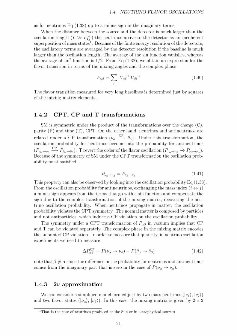
as for neutrinos Eq (1.38) up to a minus sign in the imaginary terms.
When the distance between the source and the detector is much larger than theoscillation length (L � Losc
kj ) the neutrinos arrive to the detector as an incoherentsuperposition of mass states1. Because of the finite energy resolution of the detectors,the oscillatory terms are averaged by the detector resolution if the baseline is muchlarger than the oscillation length. The average of the sin function vanishes, whereasthe average of sin2 function is 1/2. From Eq (1.38), we obtain an expression for theflavor transition in terms of the mixing angles and the complex phase
Pαβ =∑
i
|Uαi|2|Uβi|2 (1.40)
The flavor transition measured for very long baselines is determined just by squaresof the mixing matrix elements.
1.4.2 CPT, CP and T transformations
SM is symmetric under the product of the transformations over the charge (C),parity (P) and time (T), CPT. On the other hand, neutrinos and antineutrinos are
related under a CP transformation (ναCP−→ να). Under this transformation, the
oscillation probability for neutrinos become into the probability for antineutrinos
(Pνα→νβCP−→ Pνα→νβ). T revert the order of the flavor oscillation (Pνα→νβ
T−→ Pνβ→να).Because of the symmetry of SM under the CPT transformation the oscillation prob-ability must satisfied
Pνα→νβ = Pνβ→να (1.41)
This property can also be observed by looking into the oscillation probability Eq (1.38).From the oscillation probability for antineutrinos, exchanging the mass index (i↔ j)a minus sign appears from the terms that go with a sin function and compensate thesign due to the complex transformation of the mixing matrix, recovering the neu-trino oscillation probability. When neutrinos propagate in matter, the oscillationprobability violates the CPT symmetry. The normal matter is composed by particlesand not antiparticles, which induce a CP violation on the oscillation probability.
The symmetry under a CPT transformation of Pαβ in vacuum implies that CPand T can be violated separately. The complex phase in the mixing matrix encodesthe amount of CP violation. In order to measure that quantity, in neutrino oscillationexperiments we need to measure
∆PCPαβ = P (να → νβ)− P (να → νβ) (1.42)
note that β 6= α since the difference in the probability for neutrinos and antineutrinoscomes from the imaginary part that is zero in the case of P (να → να).
1.4.3 2ν approximation
We can consider a simplified model formed just by two mass neutrinos (|ν1〉, |ν2〉)and two flavor states (|να〉, |νβ〉). In this case, the mixing matrix is given by 2× 2
1That is the case of neutrinos produced at the Sun or in astrophysical sources
21
1.2 Neutrinos in the SM
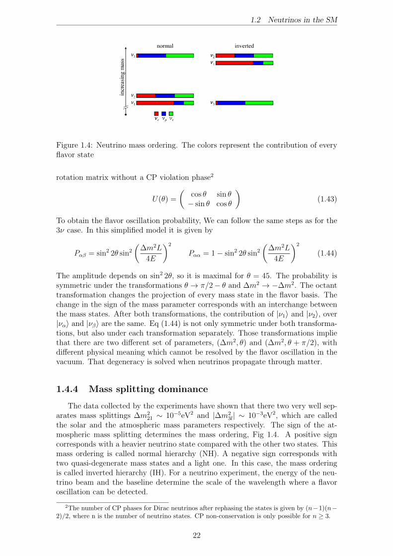
Figure 1.4: Neutrino mass ordering. The colors represent the contribution of everyflavor state
rotation matrix without a CP violation phase2
U(θ) =
(cos θ sin θ− sin θ cos θ
)(1.43)
To obtain the flavor oscillation probability, We can follow the same steps as for the3ν case. In this simplified model it is given by
Pαβ = sin2 2θ sin2
(∆m2L
4E
)2
Pαα = 1− sin2 2θ sin2
(∆m2L
4E
)2
(1.44)
The amplitude depends on sin2 2θ, so it is maximal for θ = 45. The probability issymmetric under the transformations θ → π/2− θ and ∆m2 → −∆m2. The octanttransformation changes the projection of every mass state in the flavor basis. Thechange in the sign of the mass parameter corresponds with an interchange betweenthe mass states. After both transformations, the contribution of |ν1〉 and |ν2〉, over|να〉 and |νβ〉 are the same. Eq (1.44) is not only symmetric under both transforma-tions, but also under each transformation separately. Those transformations impliethat there are two different set of parameters, (∆m2, θ) and (∆m2, θ + π/2), withdifferent physical meaning which cannot be resolved by the flavor oscillation in thevacuum. That degeneracy is solved when neutrinos propagate through matter.
1.4.4 Mass splitting dominance
The data collected by the experiments have shown that there two very well sep-arates mass splittings ∆m2
21 ∼ 10−5eV2 and |∆m23l| ∼ 10−3eV2, which are called
the solar and the atmospheric mass parameters respectively. The sign of the at-mospheric mass splitting determines the mass ordering, Fig 1.4. A positive signcorresponds with a heavier neutrino state compared with the other two states. Thismass ordering is called normal hierarchy (NH). A negative sign corresponds withtwo quasi-degenerate mass states and a light one. In this case, the mass orderingis called inverted hierarchy (IH). For a neutrino experiment, the energy of the neu-trino beam and the baseline determine the scale of the wavelength where a flavoroscillation can be detected.
2The number of CP phases for Dirac neutrinos after rephasing the states is given by (n−1)(n−2)/2, where n is the number of neutrino states. CP non-conservation is only possible for n ≥ 3.
22

1.5. NEUTRINO OSCILLATION IN MATTER
Neutrino oscillation experiments usually are devoted to the measurement of somespecific neutrino flavors oscillation over a narrow L/E ratio. Therefore, they aremainly sensitives to one the oscillation wavelengths. In the case of experiments whichare sensitives to the atmospheric mass parameter, the following approximation canbe used on the oscillation probability ∆m2
31 ≈ ∆m232 ≡ ∆m2 and ∆m2
21 ≈ 0. In thatregime, the contribution of the imaginary vanishes in Eq (1.38) and the oscillationprobability can be written as
Pαβ = δαβ − 4(δαβ|Uα3|2 − |Uα3|2|Uβ3|2) sin2
(∆m2L
4E
)(1.45)
= δαβ − sin2 2θeffαβ sin2
(∆m2L
4E
)(1.46)
where
α 6= β sin2 2θeffαβ = 4|Uα3|2|Uβ3|2
α = β sin2 2θeffαα = 4|Uα3|2(1− |Uα3|2)
Those expressions can be used to describe the flavor oscillation in experiments withatmospheric neutrinos, reactor and long-base lines experiments.
There are other experiments that are mainly sensitives to the solar mass splitting.In that case, the approximation that the imaginary terms vanish cannot be used. Inorder to obtain a simplified expression, we use the finite detector energy resolution,which average the terms that depend on the atmospheric mass splitting. In thiscase, for the disappearance channel, the initial and the final states are the same(α = β), the probability can be written as
Pαα = 1− 4|Uα2|2|Uα1|2 sin2
(∆m2
21L
4E
)− 2
(|Uα3|2|Uα1|2 + |Uα2|2|Uα2|2
)(1.47)
This expression are relevant for reactor experiments like KamLAND, where theneutrino energy is of the order of ∼ MeV and the baseline is L ∼ 100 km
1.5 Neutrino oscillation in matter
The matter that form most of the enviorments where neutrino propagation takesplace is made of electrons, protons, and neutrons, some examples are the Earth orthe Sun. That enviroments are neutral, what implies a coincidence in the numberdensity of protons and electrons. Neutrinos can interact with the quarks and leptonspresent in the matter through CC and NC, as shown in Eq (1.10), and this can affectneutrino properties. Depending on the energy mediator, the neutrino interactionscan be divided into coherent or incoherent. A coherent interaction takes place whenthe energy mediator goes to zero, and the matter as well as the neutrino kinematicalproperties are unchanged after the interaction. In an incoherent interaction, theinitial and final states are different.
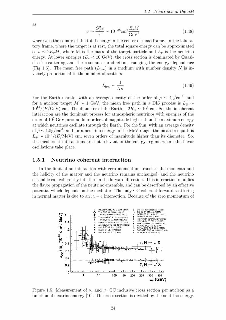
As neutrino energy increases, the total inclusive cross section in a incoherentinteraction shows a linear dependence on energy, Fig 1.5 [10]. This is the expectedresponse for a Deep Inelastic Scattering (Eν > 10 GeV), where neutrinos can scatteroff an individual quark inside a nucleon. The total cross section can be approximated
23
1.2 Neutrinos in the SM
as
σ ∼ G2F s
π∼ 10−38cm2EνM
GeV2 (1.48)
where s is the square of the total energy in the center of mass frame. In the labora-tory frame, where the target is at rest, the total square energy can be approximatedas s ∼ 2EνM , where M is the mass of the target particle and Eν is the neutrinoenergy. At lower energies (Eν < 10 GeV), the cross section is dominated by Quasi-elastic scattering and the resonance production, changing the energy dependence(Fig 1.5). The mean free path (Lfree) in a medium with number density N is in-versely proportional to the number of scatters
Lfree ∼1
Nσ(1.49)
For the Earth mantle, with an average density of the order of ρ ∼ 4g/cm3, andfor a nucleon target M ∼ 1 GeV, the mean free path in a DIS process is L⊕ ∼1014/(E/GeV) cm. The diameter of the Earth is 2R⊕ ∼ 109 cm. So, the incoherentinteraction are the dominant process for atmospheric neutrinos with energies of theorder of 105 GeV, around four orders of magnitude higher than the maximum energyat which neutrinos oscillate through the Earth. For the Sun, with an average densityof ρ ∼ 1.5g/cm3, and for a neutrino energy in the MeV range, the mean free path isL� ∼ 1018/(E/MeV) cm, seven orders of magnitude higher than its diameter. So,the incoherent interactions are not relevant in the energy regime where the flavoroscillations take place.
1.5.1 Neutrino coherent interaction
In the limit of an interaction with zero momentum transfer, the momenta andthe helicity of the matter and the neutrino remains unchanged, and the neutrinoensemble can coherently interfere in the forward direction. This interaction modifiesthe flavor propagation of the neutrino ensemble, and can be described by an effectivepotential which depends on the mediator. The only CC coherent forward scatteringin normal matter is due to an νe − e interaction. Because of the zero momentum of
Figure 1.5: Measurement of νµ and νµ CC inclusive cross section per nucleon as afunction of neutrino energy [10]. The cross section is divided by the neutrino energy.
24
1.5. NEUTRINO OSCILLATION IN MATTER
gfV gfA
e −12
+ 2 sin2 θw - 12
p 12− 2 sin2 θw
12
n −12
- 12
Table 1.3: Vector (gfV ) and axial (gfA) couplings for electrons (e), protons (p) andneutrons (n).
the mediator, the process is described by an effective hamiltonian given by
HCCeff =
GF√2νeγ
µ(1− γ5)νeeγµ(1− γ5)e (1.50)
where we have used the Fierz transformation [12] to reorder the field operators.Assuming the electron background is thermally distributed and unpolarized, we cantake the average of the hamiltonian over the electron states. The remaining effectivehamiltonian can be written as
HCCeff =
√2GFneνeLγ
0νeL (1.51)
where ne is the electron number density in the medium. This term can be interpretedas a potential energy VCC =
√2GFne for νeL due to the electrons in matter.
We can follow the same steps to derive an effective potential for the NC inter-actions. Since NC are equal for the three neutrino flavors, the effective potential isflavor independent, and it is composed of the contribution of the three interactionsνα − (e, p, n). The effective hamiltonian is given by
HNCeff =
GF√2
∑
α
(ναγµ(1− γ5)να)
∑
f=e,p,n
fγµ(gfv − γ5gfA)f (1.52)
where gfv and gfA are the vector and axial coupling constant for the fermion f (Ta-ble 1.3). After the average over the background states, the effective potential due toNC interactions is V f
NC =√
2GFnfgfV . In an electrically neutral enviroment (ne =
np) only neutrons contributes to the potential, VNC =∑
f VfNC = −
√2GFnn/2.
As a summary, neutrino evolution is modified by an effective potential oncethey propagate through matter. In an electrically neutral environment, the effectivepotential is given by
Vα =√
2GF
(neδα,e −
nn2
)(1.53)
For antineutrinos, the potential needs to be replaced by −Vα. Considering againthe Earth with a matter density of ρ ∼ 4g/cm3, the CC potential is of the order ofVCC ∼ 10−14 eV. We can compare that value with the kinetic energy term which theresponsible of the oscillation in vacuum. For a neutrino with energy Eν = 10GeVand mass ∆m2
ν ∼ 10−3eV2, the kinetic term ∆m2/2Eν ∼ 10−14 eV, similar to thematter potential.
25
1.2 Neutrinos in the SM
1.5.2 Flavor oscillation in constant matter
The evolution equation for relativistic neutrinos that propagates in matter ismodified by the matter potential term
ıd
dt
|νe〉|νµ〉|ντ 〉
=
1
2E
U
m21 0 0
0 m22 0
0 0 m23
U † +
A 0 00 0 00 0 0
|νe〉|νµ〉|ντ 〉
(1.54)
where A = 2√
2GFneE depends on the electron density and the neutrino energy.For the matter potential, we have not included the contribution from NC because itis a diagonal term, which affect in the same way to all flavors. Once the evolutionequation is solved, the NC potential contribute to the flavor evolution with a phase,similar for all flavors, that desappear when the oscillation probability is obtained.For the vacuum term, we have approximated the energy of every mass state withthe energy of the flavor states, Eq (1.36). We have also removed the contribution ofthe neutrino energy, which is equal for all mass states. The unitary matrix whichmultiplies the mass matrix is given by Eq (1.25).
As in vacuum, the mixing matrix in matter can be parameterized in terms ofthree angles and a complex phase (θ12, θ13, θ23, δ). Without loss of generality, we canrephase the states |ντ 〉 → |ντ 〉 eıδ and |ν3〉 → |ν3〉 eıδ what is equivalent to defineU = R(θ23, δCP )R(θ13)R(θ12)P , where P is a diagonal matrix that contains theMajoranna phases
U =
1 0 00 c23 s23e
−ıδcp
0 −s23e−ıδcp c23
c13 0 s13
0 1 0−s13 0 c13
c12 s12 0−s12 c12 0
0 0 1
1 0 0
0 eıδM1 0
0 0 eıδM2
(1.55)
The evolution can be solved in a intermediate basis related with the flavor basisby |ν ′i〉 =
∑α U
†αi(23, δCP ) |να〉. Once the equation is solved, the flavor evolution is
recovered multiplying by U(23, δCP ). For this reason, θ23 and δCP are not modifiedby matter evolution, and their value is the same as in vacuum.
To solve the neutrino evolution we have to specify the profile density whereneutrino propagates. For an arbitrary density profile, the only exact solution isnumerical, but there are some matter scenarios where an analytical solution can beobtained, like the constant density matter. In this case, we can define the neutrinohamiltonian (H) as
H = U
m21 0 0
0 m22 0
0 0 m23
U † +
A 0 00 0 00 0 0
(1.56)
and U as the mixing matrix that relates the flavor states with the hamiltonianeigenstates
U †HU =
λ1 0 00 λ2 00 0 λ3
(1.57)
26

1.5. NEUTRINO OSCILLATION IN MATTER
Following the same steps as in section 1.4.1, we can obtain the oscillation probability
Pαβ (L,E) = δαβ − 4∑
i>j
Re[UαiU†αjU
†βiUβj] sin2
((λi − λj)L
4E
)(1.58)
+ 2∑
i>j
Im[UαiU†αjU
†βiUβj] sin
((λi − λj)L
2E
)
The oscillation probability for a constant density profile coincides with the expressionin vacuum replacing U → U and Ei → λi.
1.5.3 2ν approximation
In a simplify scenario which consist of two flavor states |να〉 and |νβ〉, the oscil-lation is described by the mass difference between two massive states |ν1〉 and |ν2〉,and the mixing matrix Um is given by the rotation matrix
Um =
(cos θm sin θm− sin θm cos θm
)(1.59)
The evolution equation is given by
ıd
dx
(|να〉|νβ〉
)=
1
2E
[U
(m2
1 00 m2
2
)U † +
(Aα 00 Aβ
)](|να〉|νβ〉
)(1.60)
where U is the 2 × 2 rotation matrix given by Eq (1.43), and Aα = 2EVα. Thematter potential for |νµ〉 and |ντ 〉 is due to the NC interactions for both states, soin the evolution equation we can take its value as zero 3, and the evolution for thosestates is described by the vacuum equation. For any two flavor states, we can useUm to diagonalize the hamiltonian, the eigenvalues are
λ1(x) =1
2
[m2
1 +m22 + Aα + Aβ −
√(∆m2 sin 2θ)2 + (∆m2 cos 2θ − (Aα − Aβ))2
](1.61)
λ2(x) =1
2
[m2
1 +m22 + Aα + Aβ +
√(∆m2 sin 2θ)2 + (∆m2 cos 2θ − (Aα − Aβ))2
](1.62)
and the mixing angle in matter is given by
tan 2θm =∆m2 sin 2θ
∆m2 cos 2θ − 2E (Vα − Vβ)(1.63)
θm depends on the potential, so the relation between the mass and the flavor stateschange along the neutrino trajectory as the electron density change. If a massstate in vacuum, let say |ν1〉, has a large projection over a flavor state, for example|να〉, which means θ ' 0 or θ ' π/2, inside matter that verifies 2E(Vα − Vβ) �∆m2 cos 2θ, the projection change and |να〉 is dominated by |ν2〉. For some values ofthe matter potential and the neutrino energy, the denominator of tan 2θm vanishes
3The matter potential is non-zero for any of the three neutrinos defined in the SM because ofthe electroweak interactions. For the states |νµ〉 and |ντ 〉 the potential comes from the NC, so ithas the same value for both states, and it does not play a role in the oscillation probability. Ifwe consider the mixing with sterile neutrinos, since this new fermions are singlets of SM, theirmatter potential is zero, and we have to include the contribution of the NC to the potential of theleft-handed states.
27
1.2 Neutrinos in the SM
(2E(Vα−Vβ) = ∆m2 cos 2θ), and the mixing angle becomes θm = 45. At this point,there is maximal mixing, and the contribution of every mass state to every flavorstates is the same. The enhancement of the flavor mixing in matter is called MSWeffect [13, 14]. The resonance happens for θ < π/4 if Aα−Aβ and ∆m2 has the samesign or θ > π/4 in the other case. Therefore, for a given sign of ∆m2 and octant ofvacuum mixing angle, the resonance only happens for neutrinos or antineutrinos.
Neutrino wavelength also can change along its path. The energy difference (λ2−λ1), which correspond to the oscillation wavelength in matter, depends on the matterdensity and takes its smallest value (∆m2 sin 2θ) at the resonant point.
1.5.4 Adiabatic approximation
As in the 3ν mixing, solving the evolution for a constant matter potential andcomputing the oscillation probability we recover similar expressions as Eq (1.44) bychanging θ → θm and ∆m2 → (λ2 − λ1). In matter, the symmetry over the mixingangle octant in the 2ν approximation is broken, for a given sign of Aα − Aβ and∆m2, θm is larger or smaller than in vacuum depending on the octant of θ. For anon-constant profile density, the evolution equation can be written in the mass basisas
ıd
dx
(|ν1〉|ν2〉
)=
[1
2E
(λ1(x) 0
0 λ2(x)
)− ıU d
dxU †](|ν1〉|ν2〉
)(1.64)
Developing the last term in the previous equation, we find that it correspond toan antisymmetric matrix proportional to θ ≡ dθ/dx. This term implies a mixingbetween the mass states in the evolution. If θ/|λ2 − λ1| is very small, the evolutionof the mass states is independent of each other and is given by the exponential ofthe integral of λi along the neutrino path. That is called adiabatic regime and takeplace in slowly varying matter potential compared with the oscillation wavelenght,like the Sun. Under that approximation, the oscillation probability becomes
Pαβ(L) =
∣∣∣∣∣∑
i
Uβi(0)Uαi(L) exp
{− ı
2E
∫ L
0
dxλi(x)
}∣∣∣∣∣
2
(1.65)
We can study the adiabatic neutrino evolution and the oscillation probability inthe particular example of neutrinos created in the inner part of the Sun, where thematter potential can be expected to be much higher than its value at the resonace.
The two main mechanisms that create neutrinos in the Sun are the pp chainand CNO cycle, where the overall result of both process is the conversion of 4protons into a 4He nucleus, two positrons, two electron neutrinos and energy (4p→4
He + 2e+ + 2νe + γ). So, we can study the evolution of the system νe − νβ, whereνβ is a linear combination of νµ and ντ .
At the inner part of the Sun, if the matter potential verifies Ae � ∆m2 cos 2θ,the mixing angle is θm ' π/2 and the system is mainly composed by |ν2〉. Since theevolution is adiabatic, the system remains in the same mass state along the wholepath. As the neutrino moves to smaller density regions, θm become smaller and themixing increase, being the maximal mixing point at the resonance point θm = π/4.As the neutrino arrive to the outer part of the Sun, the density decrease but now thesame happen to the mixing. When neutrino exit from the Sun, the |νβ〉 componentis fixed by the vacuum mixing angle, θ.
We can compute the disappearance probability (Pee) from Eq (1.65). Notice thatUei(0) correspond to the mixing matrix at the production point and, Uei(L) outside
28
1.6. ATMOSPHERIC NEUTRINOS
the sun
Pee =1
2
[1 + cos 2θm cos 2θ + sin 2θm sin 2θ cos
(−ı2E
∫ L
0
dx(λ2(x)− λ1(x))
)]
(1.66)we have pulled out the phase associated to λ1. θm and θ are the mixing angles atthe production point and outside the Sun, respectively. Due to the large radius ofthe Sun and the small energy of the neutrinos created, the oscillatory term is goingto be averaged. Using θm ' π/2 the probability becomes
Pee = sin2 θ (1.67)
After crossing the Sun, the probability to obtain a νe can be very small, and it is justdetermined by the vacuum mixing angle. Since the final probability is independentof the energy and the distance traveled, the νe disappearance can be explained byflavor transition rather than a flavor oscillation.
1.6 Atmospheric neutrinos
As it was mentioned at the begining, atmospheric neutrinos are created in thecollision of cosmic rays with the atmospheric nuclei. Coming from outside the solarsystem, their energy range extends from 100 MeV, below which energy the flux ofextraterrestrial particles arriving to the Earth is dominated by the solar wind, upto 1020 eV, above which the flux is suppressed because of the interaction with thecosmic microwave background (cmb). The cosmic rays are mainly protons, electronsand a small fraction of heavy nuclei [15]. After the interactaion with the atmosphere,a second generation of particles is produced, and among the hadrons produced thereare many pions and kaons. The spectrum of this secondary flux peaks in the GeVrange, and can be approximated by a power-law to higher energies. At energies lowerthan 100 GeV, the atmospheric neutrino flux is dominated by the π decay, Eq (1.68),whose principal mode corresponds with the decay into a µ and a νµ with a branchingratio (Br) of Br = 99.99% [10]. To higher energies, the K decay contributiondominates. Apart from the K decay into µ and νµ Eq (1.68) that correspond to aBr = 63.56% [10], there are additional contributions from other semileptonic decayslike K± → π0 + µ± + νµ(νµ) (K± → π0 + e± + νe(νe)) with a Br = 3.35%(5.07%).There is a secondary neutrino flux generated by the µ decay Eq (1.68) that contributein the same amount to νµ and νe fluxes. So, the atmospheric neutrino flux is formedby νµ and νe in a flavor ratio (νµ + νµ)/(νe + νe) ' 2. At high energies, this flux issuppressed because µ hit the Earth before its decay.
π± → µ± + νµ(νµ) Br = 99, 99% (1.68)
K± → µ± + νµ(νµ) Br = 63.56%
µ± → e± + νe(νe) + νµ(νµ) Br = 100%
The first observation of atmospheric neutrinos was carried out in 1960’s by theKolar Gold Field experiment in India [16] and the underground experiments in SouthAfrica [17]. Both experiments measured the horizontal flux because they could notdistinguish between the up and down directions. In the following decades, new
29
1.2 Neutrinos in the SM
experiments were able to measure the atmospheric neutrino flux with high precision,showing a dependence of the flux that arrives at the detector not only with the rateat which they are produced but also with the distance traveled along the Earth.
1.6.1 Atmospheric neutrino flux calculations
A detailed knowledge of the neutrino flux is crucial to determine their oscillationproperties. The most recent calculations of the atmospheric neutrino flux are basedin 3D-MonteCarlo (MC) simulations, where the motion of all the cosmic rays thatpenetrate the Earth magnetic field is followed, as well as the subsequent generationsof particles, created after their interaction. All the neutrinos generated during thepropagation, whose direction cross a specific location in the Earth, are registered.
The MC simulation makes a convolution between the primary cosmic ray spec-trum (φp), the yield (Y ) of neutrinos per primary particle and the geomagneticcutoff (R) [15]
φνi = φp ⊗Rp ⊗ Yp→νi +∑
A
φA ⊗RA ⊗ YA→νi (1.69)
where A corresponds to the heavy nuclei present in the arriving cosmic ray flux. φνishows an energy dependence that follows a power law φνi ∼ Eγ
ν (Fig 1.6), with anspectral index close to γ ≈ −3 in the energy range 1 GeV to 1 TeV. For higher (lower)energies the flux becomes steeper (less marked). About the zenith response, theflux shape depends on the energy and the Earth location where it is computed [18](Fig 1.6). Those effects are due to:
- Geomagnetic effects over the cosmic ray fluxes. Earth magnetic field modifiesthe trajectory of the charged cosmic rays once they arrive to the Earth. Theeffect depends on the impact point over the Earth. Low rigidity particles canonly penetrate to the Earth in the parallel direction to the magnetic field. Forhigh rigidity, cosmic rays can enter to Earth from any direction.
- A zenith dependence of the yield. Inclined showers develops in air longerdistances before hitting the ground, and therefore they have more time todecay. The atmosphere density increase as the altitude decrease. For theinclined shower, a longer part of the track is developed in high altitudes, whichincrease the probability that the particles of the showers end in a decay. Thoseeffects are more relevant for high energy neutrinos. For low energies, neutrinosare produced in the decays of low energy mesons and muons, for those whothere is no enhancement in the horizontal directions. As a results, the ratiobetween the flux from horizontal to vertical directions increase with neutrinoenergy.
- Enhancement of the flux at horizontal directions due to the spherical geometryof the atmosphere. For low energy neutrinos, there is no correlation betweenneutrino direction and its parent particle, the neutrino emission is isotropic.For an observer which is not at the center of the emission sphere, the centerof the Earth, there is an enhancement in the horizontal direction. The effectis stronger as the observer moves away from the center. For high energies, theisotropy emission disappear and the neutrino direction can be approximatedby its parent direction, and the enhancement disappears.
30

1.6. ATMOSPHERIC NEUTRINOS
-1 -0.5 0 0.5 1cosθ
z
0.1
1
dφν/d
E (
cm-2
s-1Sr
-1G
eV-1
)Eν = 0.3 GeVEν = 10 GeV
0.1 1 10 100 1000Eν (GeV)
10-5
10-4
10-3
10-2
10-1
(dφ ν/d
E)
x E
2 (cm
-2s-1
Sr-1
GeV
) Figure 1.6: Atmospheric muon neutrino flux (φνµ) as a function of zenit angle (left)and neutrino energy (right). The dash line in the left pannel has been increase by 3orders of magnitude. The flux has been obtain from the tables published in [19]
All those effects are presented in the left panel of Fig 1.6, that shows the muonatmospheric neutrino flux for two different energies Eν = 0.3 GeV (continuous line)and Eν = 10 GeV (dashed line) as a function of the zenith angle. Due to thestronger energy dependence od the flux, the dash line has been increased by 3orders of magnitude. For the continuous line, the flux is higher for the horizontaldirection because of the atmospheric geometry, and it has different values for the upand down directions due to the geomagnetic effects. For the dashed line, the fluxis perfectly symmetric around an axis pointing in the horizontal direction, and theflux is higher for cos θz = 0 because of the zenith dependence of the yield. The fluxhas been obtained from the tables published in [19]
1.6.2 Flavor oscillation in the Earth
The most accurate description of the Earth density profile is given by PreliminaryReference Earth Model [20] (PREM), Fig 1.7. Based in seismological studies, PREMdivides the Earth into eleven concentric spherical layers. In each of them, the densityis given in terms of the distance to the center of the Earth by a polynomial function.In that model, the neutron/electron ratio is also fixed to Yn = 1.012 in the mantleand Yn = 1.137 in the Core. Because the Earth matter is electrically neutral, usingthe density ρ and Yn can be obtained the electron density Ne = ρ/(1 + Yn). Apartfrom the density, PREM also provides values for elastic properties, attenuation andpressure.
Neutrino propagation through the Earth can only be described in the non-adiabatic regime. The Earth profile density present two very well separate den-sity regions, the mantle (|x| > 0.54) and the core (|x| < 0.54), where the densityabruptly change by a factor of two, breaking any possible adiabatic description forthe trajectories that cross the core, Fig 1.7. x is the ratio between the distanceof the layer to the center of the Earth (R) and the Earth radius R⊕ = 6371 km.Although there are analytic approximations that provide an accurate description ofthe flavor oscillation in non-adiabatic evolutions [21], we are going to proceed by a
31

1.2 Neutrinos in the SM
numerical integration in order to describe the flavor evolution.
-1 -0.8 -0.6 -0.4 -0.2 0 0.2 0.4 0.6 0.8 1x
0
2
4
6
8
10
12
14
ρ(g/
cm3 )
Figure 1.7: Earth density given by PREM [20] as a function of the fractional distanceto the Earth center x = R/R⊕, where R is the distance of the layer to the center ofthe Earth and R⊕ = 6371 km.
In order to have an overall view of the matter resonances when neutrinos travelthrough the Earth, we are going to study the electron disappearance channel, (1−Pee = Pµe + Pτe), Fig 1.8. Notice that the Earth profile density is symmetric aboutthe midpoint in the neutrino path, so the oscillation probability is invariant underthe time ordering operation Pαβ = Pβα. The flavor oscillation along the Earthdepends on neutrino energy (Eν) and the direction of the neutrino trajectory, thatis given by the cosine of the zenith angle (cos θz), defined as cos θz = −1 for up-goingneutrinos, and cos θz = 1 for down going neutrinos. To present the probability weare going to use the oscillogram, a two dimensional contour plot where every colorline corresponds with a value for 1 − Pee. In this figure, the best fit values ofthe global fit [22] were used as input for the oscillation parameters. Since we areinterested only in the evolution through the Earth, the zenith angle is in the intervalcos θz ∈ [−1, 0], for positives values the neutrino only crosses the atmosphere. Forsimplicity, we have assumed that neutrinos are produced at an altitude of 15 km4.For the energy, we have considered the range Eν ∈ [0.05, 100] GeV. At the top ofthe energy range, the flavor oscillation is limited by the atmospheric mass splitting(∼ 10−3eV2), which produce the first oscillation maximum at Eν ≈ 20 GeV. At thebottom of the energy range, neutrinos never stop oscillating. We can consider as aminimum value, the energy at which the solar mass splitting (∼ 10−5eV2) producea complete oscillation for horizontal neutrinos (cos θz = 0) inside the atmosphere isEν ≈ 0.05 GeV.
4Most of the neutrinos are produced at an altitude of 20-10 km [15]. In order to properly treatwith the neutrino production at different altitudes, we have to average the oscillation probabilityalong the atmosphere weighted by an altitude distribution function normalized to one. Due to thesmall size of the atmosphere compared with the Earth, we have fixed its size to an intermediatevalue of 15 km.
32

1.6. ATMOSPHERIC NEUTRINOS
Figure 1.8: 1−Pee for atmospheric neutrinos (left) and antineutrinos (right) crossingthe Earth.
The neutrino evolution inside the Earth is obtained by solving Eq (1.54) forPREM, Fig 1.7. 1− Pee shows two separate regions that correspond to trajectoriesthat cross the Earth core (cosθz < −0.83), or trajectories developed just in the man-tle. In a 3ν mixing, there are two oscillations wavelengths that compete at differentenergy scales. For the 1-3 mixing, the MSW resonance is driven by the atmosphericmass parameter (∆m2
31 = 2.494×10⁻³eV2 NH or ∆m232 = −2.465×10⁻³eV2 IH) [22].
A constant density approximation can be used to describe the evolution of trajec-tories that only cross the mantle [23, 24]. In this case, the resonance condition canbe written as
2VCCERν = |∆m2
3l| cos 2θ13 (1.70)
where VCC is the averaged CC potential along the neutrino path. This expressiondetermines the values of the energy where oscillation amplitude is maximal as afunction of the trajectory ER
ν (θz). In addition, to get a maximum in the oscilla-tion probability (1 − Pee ' 1), it is needed that the oscillation phase should beproportional to π/2. From Eq (1.58) we get
(λ3 − λ1)L
4E= (2k + 1)
π
2k ∈ N (1.71)
For an average density of the mantle about ρ ∼ (4− 5)g/cm3, both conditions meetat ER
ν ∼ 6 GeV and cos θz ∼ −0.8. There is only one point where both conditionsmeet because of the oscillation length at the resonance, given by
LOSCR =
LOSC
sin 2θ13
(1.72)
where LOSC is the oscillation vacuum length, which is of the order of the Earthradius. Due to the small value of θ13 ∼ 8.5 [22], LOSC
R is much longer than Earthsize.
For the 1-2 mixing, the resonant amplitude depends on the solar mass param-eter, ∆m2
21 = 7.4 × 10⁻⁵eV2 [22]. Using the approximation of constant density
33
1.2 Neutrinos in the SM
matter for the mantle, the resonant energy is about ERν ∼ 0.1 GeV. Around that
value, there are three directions where there is a total flavor conversion, cos θz ={−0.75,−0.49,−0.15}. For the solar mass parameter, the vacuum oscillation lengthis about half of the Earth radius, so at the resonance LOSC
R ∼ R⊕/4. The neu-trino baseline through the Earth can be approximated as L ' 2R⊕| cos θz|. Wecan compute the phase (φ = ∆m2
21 sin 2θ21L/4E) for the three directions where themaximum transition is obtained, finding
φ(cos θz = −0.75) ≈ 5π/2
φ(cos θz = −0.49) ≈ 3π/2
φ(cos θz = −0.15) ≈ π/2
The three directions corresponding to the first three odd multiples of π/2. Thereis another maximum transition point around cos θz ' −0.92 and Eν ' 0.2 GeV.That direction crosses the Earth core, so the evolution cannot be described by theconstant matter approximation. In spite of that, the resonant energy for the coreshould be smaller than in mantle since the matter potential is higher in the core.For that reason, a maximum transition point at the core with Eν > 0.1 GeV cannotbe explained as coincident between the resonant amplitude and phase conditions.Instead, this total flavor conversion can be explained by a parametric enhancementof the oscillations [24].
In Fig 1.8 we have used a normal mass ordering, since the best fit points towardsthat mass distribution, although with small preference over invert hierarchy [22].Since the mass splittings and the matter potential for antineutrinos have oppositesigns, it is not possible to get a resonant amplitude for them. We can repeat thesimulation for IH, and we will get the opposite situation, the maximum flavor con-version will take place for antineutrinos. For IH, we can repeat the same discussionas before, but in this case for antineutrinos.
1.6.3 IceCube DeepCore experiment
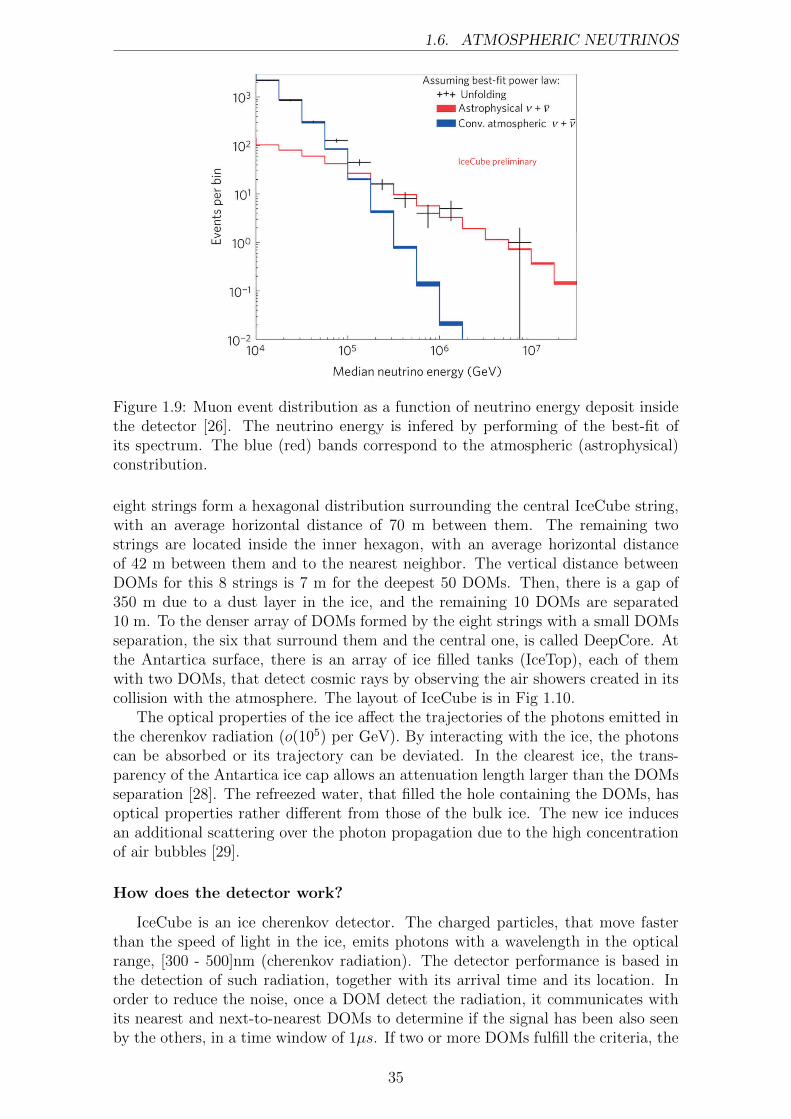
IceCube is neutrino cherenkov telescope located at the South Pole, whose primaryscientific objective is the discovery of astrophysical neutrinos, which was realized in2013 [25]. The astrophysical flux measured is in the energy range of ∼ 30 TeVto PeV, Fig. 1.9. For lower energies, the neutrino flux arriving at the detector isdominated by atmospheric neutrinos. At sufficient low energies, the atmosphericflux can be measured for an L/E ratio relevant for the flavor oscillations, openingthe possibility to study this phenomenon for high energy atmospheric neutrinos.Before this experiment, SK was the only statistically significant detector able tomeasure oscillations through the Earth.
The small neutrino cross section and the expected low flux for astrophysicalneutrinos require a detector with a large target mass. IceCube consists of 5160photomultipliers, called DOMs (Digital Optical Module) distributed over a volumeof almost a cubic kilometer below the Antartica surface, which is equivalent to a massof∼ 1000 MTon. The DOMs are arranged in 86 strings distributed along a hexagonalpattern [27]. Each string contains 60 DOMs and, 78 of them are instrumented froma depth of ∼ 1450 km to ∼ 2450 km, with a vertical spacing of 17 m between DOM,and a horizontal distance of 125 m to the nearest string. The remaining eight stringsare also formed by 60 photomultipliers with 35% higher efficiency. Six of the last
34
1.6. ATMOSPHERIC NEUTRINOS
Figure 1.9: Muon event distribution as a function of neutrino energy deposit insidethe detector [26]. The neutrino energy is infered by performing of the best-fit ofits spectrum. The blue (red) bands correspond to the atmospheric (astrophysical)constribution.
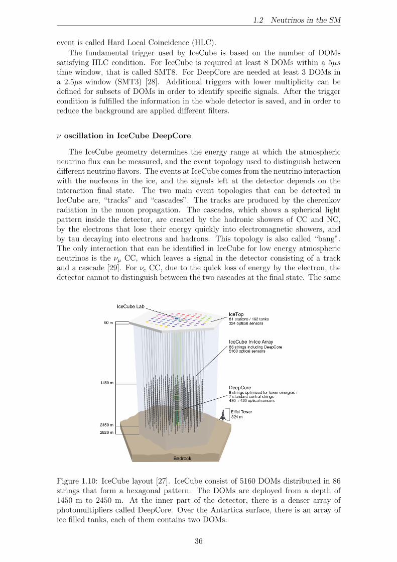
eight strings form a hexagonal distribution surrounding the central IceCube string,with an average horizontal distance of 70 m between them. The remaining twostrings are located inside the inner hexagon, with an average horizontal distanceof 42 m between them and to the nearest neighbor. The vertical distance betweenDOMs for this 8 strings is 7 m for the deepest 50 DOMs. Then, there is a gap of350 m due to a dust layer in the ice, and the remaining 10 DOMs are separated10 m. To the denser array of DOMs formed by the eight strings with a small DOMsseparation, the six that surround them and the central one, is called DeepCore. Atthe Antartica surface, there is an array of ice filled tanks (IceTop), each of themwith two DOMs, that detect cosmic rays by observing the air showers created in itscollision with the atmosphere. The layout of IceCube is in Fig 1.10.
The optical properties of the ice affect the trajectories of the photons emitted inthe cherenkov radiation (o(105) per GeV). By interacting with the ice, the photonscan be absorbed or its trajectory can be deviated. In the clearest ice, the trans-parency of the Antartica ice cap allows an attenuation length larger than the DOMsseparation [28]. The refreezed water, that filled the hole containing the DOMs, hasoptical properties rather different from those of the bulk ice. The new ice inducesan additional scattering over the photon propagation due to the high concentrationof air bubbles [29].
How does the detector work?
IceCube is an ice cherenkov detector. The charged particles, that move fasterthan the speed of light in the ice, emits photons with a wavelength in the opticalrange, [300 - 500]nm (cherenkov radiation). The detector performance is based inthe detection of such radiation, together with its arrival time and its location. Inorder to reduce the noise, once a DOM detect the radiation, it communicates withits nearest and next-to-nearest DOMs to determine if the signal has been also seenby the others, in a time window of 1µs. If two or more DOMs fulfill the criteria, the
35
1.2 Neutrinos in the SM
event is called Hard Local Coincidence (HLC).
The fundamental trigger used by IceCube is based on the number of DOMssatisfying HLC condition. For IceCube is required at least 8 DOMs within a 5µstime window, that is called SMT8. For DeepCore are needed at least 3 DOMs ina 2.5µs window (SMT3) [28]. Additional triggers with lower multiplicity can bedefined for subsets of DOMs in order to identify specific signals. After the triggercondition is fulfilled the information in the whole detector is saved, and in order toreduce the background are applied different filters.
ν oscillation in IceCube DeepCore
The IceCube geometry determines the energy range at which the atmosphericneutrino flux can be measured, and the event topology used to distinguish betweendifferent neutrino flavors. The events at IceCube comes from the neutrino interactionwith the nucleons in the ice, and the signals left at the detector depends on theinteraction final state. The two main event topologies that can be detected inIceCube are, “tracks” and “cascades”. The tracks are produced by the cherenkovradiation in the muon propagation. The cascades, which shows a spherical lightpattern inside the detector, are created by the hadronic showers of CC and NC,by the electrons that lose their energy quickly into electromagnetic showers, andby tau decaying into electrons and hadrons. This topology is also called “bang”.The only interaction that can be identified in IceCube for low energy atmosphericneutrinos is the νµ CC, which leaves a signal in the detector consisting of a trackand a cascade [29]. For νe CC, due to the quick loss of energy by the electron, thedetector cannot to distinguish between the two cascades at the final state. The same
Figure 1.10: IceCube layout [27]. IceCube consist of 5160 DOMs distributed in 86strings that form a hexagonal pattern. The DOMs are deployed from a depth of1450 m to 2450 m. At the inner part of the detector, there is a denser array ofphotomultipliers called DeepCore. Over the Antartica surface, there is an array ofice filled tanks, each of them contains two DOMs.
36
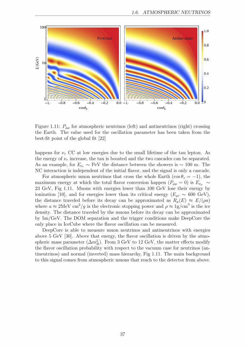
1.6. ATMOSPHERIC NEUTRINOS
Figure 1.11: Pµµ for atmospheric neutrinos (left) and antineutrinos (right) crossingthe Earth. The value used for the oscillation parameter has been taken from thebest-fit point of the global fit [22]
happens for ντ CC at low energies due to the small lifetime of the tau lepton. Asthe energy of ντ increase, the tau is boosted and the two cascades can be separated.As an example, for Eντ ∼ PeV the distance between the showers is ∼ 100 m. TheNC interaction is independent of the initial flavor, and the signal is only a cascade.
For atmospheric muon neutrinos that cross the whole Earth (cos θz = −1), themaximum energy at which the total flavor conversion happen (Pµµ = 0) is Eνµ ∼23 GeV, Fig 1.11. Muons with energies lower than 100 GeV lose their energy byionization [10], and for energies lower than its critical energy (Eµc ∼ 600 GeV),the distance traveled before its decay can be approximated as Rµ(E) ≈ E/(ρa)where a ≈ 2MeV cm2/g is the electronic stopping power and ρ ≈ 1g/cm3 is the icedensity. The distance traveled by the muons before its decay can be approximatedby 5m/GeV. The DOM separation and the trigger conditions make DeepCore theonly place in IceCube where the flavor oscillation can be measured.
DeepCore is able to measure muon neutrinos and antineutrinos with energiesabove 5 GeV [30]. Above that energy, the flavor oscillation is driven by the atmo-spheric mass parameter (∆m2
3l). From 3 GeV to 12 GeV, the matter effects modifythe flavor oscillation probability with respect to the vacuum case for neutrinos (an-tineutrinos) and normal (inverted) mass hierarchy, Fig 1.11. The main backgroundto this signal comes from atmospheric muons that reach to the detector from above.
37

1.2 Neutrinos in the SM
38
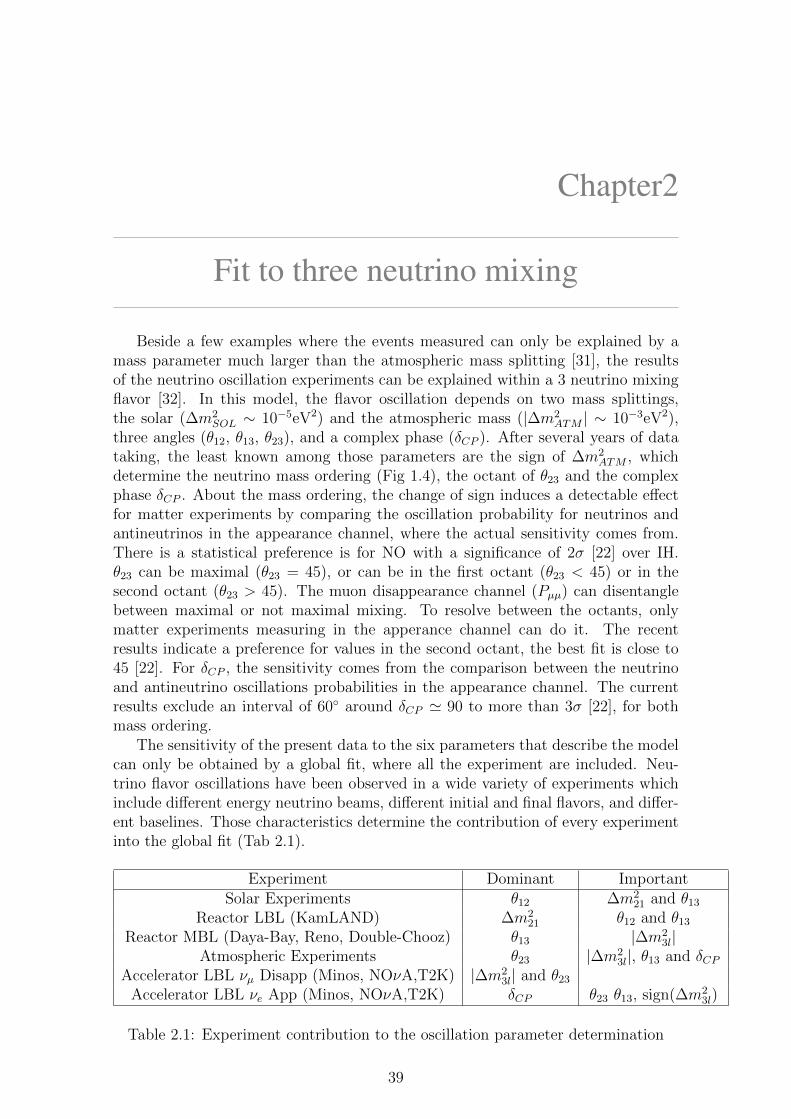
Chapter2
Fit to three neutrino mixing
Beside a few examples where the events measured can only be explained by amass parameter much larger than the atmospheric mass splitting [31], the resultsof the neutrino oscillation experiments can be explained within a 3 neutrino mixingflavor [32]. In this model, the flavor oscillation depends on two mass splittings,the solar (∆m2
SOL ∼ 10−5eV2) and the atmospheric mass (|∆m2ATM | ∼ 10−3eV2),
three angles (θ12, θ13, θ23), and a complex phase (δCP ). After several years of datataking, the least known among those parameters are the sign of ∆m2
ATM , whichdetermine the neutrino mass ordering (Fig 1.4), the octant of θ23 and the complexphase δCP . About the mass ordering, the change of sign induces a detectable effectfor matter experiments by comparing the oscillation probability for neutrinos andantineutrinos in the appearance channel, where the actual sensitivity comes from.There is a statistical preference is for NO with a significance of 2σ [22] over IH.θ23 can be maximal (θ23 = 45), or can be in the first octant (θ23 < 45) or in thesecond octant (θ23 > 45). The muon disappearance channel (Pµµ) can disentanglebetween maximal or not maximal mixing. To resolve between the octants, onlymatter experiments measuring in the apperance channel can do it. The recentresults indicate a preference for values in the second octant, the best fit is close to45 [22]. For δCP , the sensitivity comes from the comparison between the neutrinoand antineutrino oscillations probabilities in the appearance channel. The currentresults exclude an interval of 60◦ around δCP ' 90 to more than 3σ [22], for bothmass ordering.
The sensitivity of the present data to the six parameters that describe the modelcan only be obtained by a global fit, where all the experiment are included. Neu-trino flavor oscillations have been observed in a wide variety of experiments whichinclude different energy neutrino beams, different initial and final flavors, and differ-ent baselines. Those characteristics determine the contribution of every experimentinto the global fit (Tab 2.1).
Experiment Dominant ImportantSolar Experiments θ12 ∆m2
21 and θ13
Reactor LBL (KamLAND) ∆m221 θ12 and θ13
Reactor MBL (Daya-Bay, Reno, Double-Chooz) θ13 |∆m23l|
Atmospheric Experiments θ23 |∆m23l|, θ13 and δCP
Accelerator LBL νµ Disapp (Minos, NOνA,T2K) |∆m23l| and θ23
Accelerator LBL νe App (Minos, NOνA,T2K) δCP θ23 θ13, sign(∆m23l)
Table 2.1: Experiment contribution to the oscillation parameter determination
39
JHEP01(2017)087
Published for SISSA by Springer
Received: November 16, 2016
Revised: January 3, 2017
Accepted: January 14, 2017
Published: January 20, 2017
Updated fit to three neutrino mixing: exploring the
accelerator-reactor complementarity
Ivan Esteban,a M.C. Gonzalez-Garcia,a,b,c Michele Maltoni,d Ivan Martinez-Solerd
and Thomas Schwetze
aDepartament de Fisıca Quantica i Astrofısica and Institut de Ciencies del Cosmos,
Universitat de Barcelona, Diagonal 647, E-08028 Barcelona, SpainbInstitucio Catalana de Recerca i Estudis Avancats (ICREA),
Pg. Lluis Companys 23, 08010 Barcelona, SpaincC.N. Yang Institute for Theoretical Physics, State University of New York at Stony Brook,
Stony Brook, NY 11794-3840, U.S.A.dInstituto de Fısica Teorica UAM/CSIC, Universidad Autonoma de Madrid,
Calle de Nicolas Cabrera 13–15, Cantoblanco, E-28049 Madrid, SpaineInstitut fur Kernphysik, Karlsruher Institut fur Technologie (KIT),
D-76021 Karlsruhe, Germany
E-mail: [email protected],
[email protected], [email protected],
[email protected], [email protected]
Abstract: We perform a combined fit to global neutrino oscillation data available as of
fall 2016 in the scenario of three-neutrino oscillations and present updated allowed ranges
of the six oscillation parameters. We discuss the differences arising between the consistent
combination of the data samples from accelerator and reactor experiments compared to
partial combinations. We quantify the confidence in the determination of the less precisely
known parameters θ23, δCP, and the neutrino mass ordering by performing a Monte Carlo
study of the long baseline accelerator and reactor data. We find that the sensitivity to the
mass ordering and the θ23 octant is below 1σ. Maximal θ23 mixing is allowed at slightly
more than 90% CL. The best fit for the CP violating phase is around 270◦, CP conservation
is allowed at slightly above 1σ, and values of δCP ' 90◦ are disfavored at around 99% CL
for normal ordering and higher CL for inverted ordering.
Keywords: Neutrino Physics, Solar and Atmospheric Neutrinos
ArXiv ePrint: 1611.01514
Open Access, c© The Authors.
Article funded by SCOAP3.doi:10.1007/JHEP01(2017)087

JHEP01(2017)087
Contents
1 Introduction 1
2 Global analysis: determination of oscillation parameters 2
2.1 Data samples analyzed 2
2.2 Results: oscillation parameters 3
2.3 Results: leptonic mixing matrix and CP violation 6
3 Issues in present analysis 8
3.1 Status of ∆m221 in solar experiments versus KamLAND 8
3.2 ∆m23` determination in LBL accelerator experiments versus reactors 9
3.2.1 Impact on the determination of θ23, mass ordering, and δCP 11
3.3 Analysis of Super-Kamiokande atmospheric data 15
4 Monte Carlo evaluation of confidence levels for θ23, δCP and ordering 17
4.1 δCP and the mass ordering 19
4.2 θ23 and the mass ordering 22
5 Conclusions 24
A List of data used in the analysis 25
1 Introduction
Experiments measuring the flavor composition of solar neutrinos, atmospheric neutrinos,
neutrinos produced in nuclear reactors and in accelerators have established that lepton fla-
vor is not conserved in neutrino propagation, but it oscillates with a wavelength depending
on distance and energy, because neutrinos are massive and the mass states are admixtures
of the flavor states [1, 2], see ref. [3] for an overview.
With the exception of a set of unconfirmed “hints” of possible eV scale mass states
(see ref. [4] for a recent review), all the oscillation signatures can be explained with the
three flavor neutrinos (νe, νµ, ντ ), which can be expressed as quantum superpositions of
three massive states νi (i = 1, 2, 3) with masses mi. This implies the presence of a leptonic
mixing matrix in the weak charged current interactions [5, 6] which can be parametrized as:
U =
1 0 0
0 c23 s23
0 −s23 c23
· c13 0 s13e
−iδCP
0 1 0
−s13eiδCP 0 c13
· c12 s12 0
−s12 c12 0
0 0 1
· P (1.1)
where cij ≡ cos θij and sij ≡ sin θij . The angles θij can be taken without loss of generality
to lie in the first quadrant, θij ∈ [0, π/2], and the phase δCP ∈ [0, 2π]. Here P is a diagonal
– 1 –
JHEP01(2017)087
matrix which is the identity if neutrinos are Dirac fermions and it contains two additional
phases if they are Majorana fermions, and plays no role in neutrino oscillations [7, 8]. In
this convention there are two non-equivalent orderings for the neutrino masses which can be
chosen to be: normal ordering (NO) with m1 < m2 < m3, and inverted ordering (IO) with
m3 < m1 < m2. Furthermore the data shows a relatively large hierarchy between the mass
splittings, ∆m221 � |∆m2
31| ' |∆m232| with ∆m2
ij ≡ m2i −m2
j . In this work we follow the
convention introduced in ref. [9] and present our results in terms of the variable ∆m23`, with
` = 1 for NO and ` = 2 for IO. Hence, ∆m23` = ∆m2
31 > 0 for NO and ∆m23` = ∆m2
32 < 0
for IO, i.e., it corresponds to the mass splitting with the largest absolute value.
In this article, we present an up-to-date (as of fall 2016) global analysis of neutrino
data in the framework of three-neutrino oscillations. Alternative recent global fits have
been presented in refs. [10, 11]. With current data from the accelerator long-baseline
experiments MINOS, T2K, NOνA and modern reactor experiments like Daya-Bay, RENO,
and Double-Chooz, their complementarity anticipated more than a decade ago [12–14] has
become a reality, and the combined analysis starts to show some sensitivity to subtle effects
like the θ23 octant or the δCP phase (though still at low statistical significance).
The outline of the paper is as follows: in section 2.1 we describe the data samples
included in our analysis (see also appendix A for a schematic list). The presently allowed
ranges of the six oscillation parameters are given in section 2.2 assuming that ∆χ2 follows
a χ2-distribution, while section 2.3 contains the corresponding measures of CP violation in
terms of the leptonic Jarlskog invariant and the leptonic unitarity triangle. Deviations from
the Gaussian approximation of the confidence intervals for θ23 and δCP and the confidence
level for the mass ordering determination are quantified in section 4. Several issues ap-
pearing in the present analysis are discussed in section 3, in particular about the consistent
combination of results from long baseline accelerator experiments with reactors results,
now that both provide comparable precision in the determination of the relevant mass-
squared difference. We also give the updated status on the ongoing tension in the ∆m221
determination from solar experiments versus KamLAND, and comment on the stand-by in
the analysis of the Super-Kamiokande atmospheric data. Section 5 contains the summary
of our results.
2 Global analysis: determination of oscillation parameters
2.1 Data samples analyzed
In the analysis of solar neutrino data we consider the total rates from the radiochemical
experiments Chlorine [15], Gallex/GNO [16] and SAGE [17], the results for the four phases
of Super-Kamiokande [18–22], the data of the three phases of SNO included in the form
of the parametrization presented in [23], and the results of both Phase-I and Phase-II of
Borexino [24–26].
Results from long baseline (LBL) accelerator experiments include the final energy
distribution of events from MINOS [27, 28] in νµ and νµ disappearance and νe and νeappearance channels, as well as the latest energy spectrum for T2K in the same four chan-
nels [29, 30] and for NOνA on the νµ disappearance and νe appearance neutrino modes [31].
– 2 –
JHEP01(2017)087
Data samples on νe disappearance from reactor include the full results of the long
baseline reactor data in KamLAND [32], as well as the results from medium baseline reactor
experiments from CHOOZ [33] and Palo Verde [34]. Concerning running experiments we
include the latest spectral data from Double-Chooz [35] and Daya-Bay [36], while for RENO
we use the total rates obtained with their largest data sample corresponding to 800 days
of data-taking [37].
In the analysis of the reactor data, the unoscillated reactor flux is determined as de-
scribed in [38] by including in the fit the results from short baseline reactor data (RSBL)
from ILL [39], Gosgen [40], Krasnoyarsk [41, 42], ROVNO88 [43], ROVNO4 [44], Bugey3 [45],
Bugey4 [46], and SRP [47].
For the analysis of atmospheric neutrinos we include the results from IceCube/DeepCore
3-year data [48].
The above data sets constitute the samples included in our NuFIT 3.0 analysis. For
Super-Kamiokande atmospheric neutrino data from phases SK1–4 we will comment on our
strategy in section 3.3. A full list of experiments including the counting of data points in
each sample can be found in appendix A.
2.2 Results: oscillation parameters
The results of our standard analysis are presented in figures 1 and 2 where we show projec-
tions of the allowed six-dimensional parameter space.1 In all cases when including reactor
experiments we leave the normalization of reactor fluxes free and include data from short-
baseline (less than 100 m) reactor experiments. In our previous analysis [9, 50] we studied
the impact of this choice versus that of fixing the reactor fluxes to the prediction of the
latest calculations [51–53]. As expected, the overall description is better when the flux
normalization fflux is fitted against the data. We find χ2(fflux fix)−χ2(fflux fit) ' 6 which
is just another way to quantify the well-known short baseline reactor anomaly to be ∼ 2.5σ.
However, the difference in the resulting parameter determination (in particular for θ13) be-
tween these two reactor flux normalization choices has become marginal, since data from
the reactor experiments with near detectors such as Daya-Bay, RENO and Double-Chooz
(for which the near-far comparison allows for flux-normalization independent analysis) is
now dominant. Consequently, in what follows we show only the ∆χ2 projections for our
standard choice with fitted reactor flux normalization.
The best fit values and the derived ranges for the six parameters at the 1σ (3σ) level
are given in table 1. For each parameter x the ranges are obtained after marginalizing with
respect to the other parameters2 and under the assumption that ∆χ2marg(x) follows a χ2
distribution. Hence the 1σ (3σ) ranges are given by the condition ∆χ2marg(x) = 1 (9). It
is known that because of its periodic nature and the presence of parameter degeneracies
the statistical distribution of the marginalized ∆χ2 for δCP and θ23 (and consequently the
1∆χ2 tables from the global analysis corresponding to all 1-dimensional and 2-dimensional projections
are available for download at the NuFIT website [49].2In this paper we use the term “marginalization” over a given parameter as synonym for minimizing the
χ2 function with respect to that parameter.
– 3 –
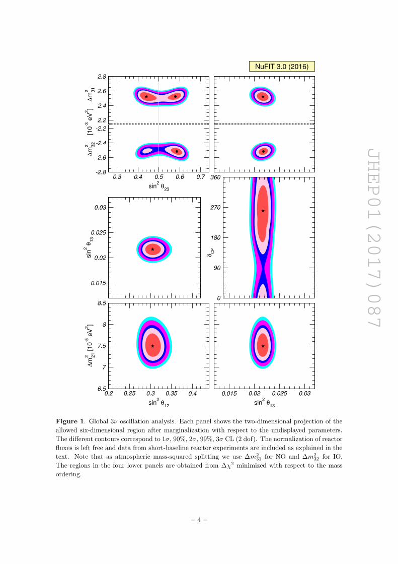
JHEP01(2017)087
★
0.2 0.25 0.3 0.35 0.4
sin2
θ12
6.5
7
7.5
8
8.5
∆m
2 21 [
10
-5 e
V2]
★
0.015 0.02 0.025 0.03
sin2
θ13
★
0.015
0.02
0.025
0.03
sin
2θ
13
★
0
90
180
270
360
δC
P
0.3 0.4 0.5 0.6 0.7
sin2
θ23
-2.8
-2.6
-2.4
-2.2
★
2.2
2.4
2.6
2.8
∆m
2 32
[1
0-3
eV
2]
∆
m2 3
1★
NuFIT 3.0 (2016)
Figure 1. Global 3ν oscillation analysis. Each panel shows the two-dimensional projection of the
allowed six-dimensional region after marginalization with respect to the undisplayed parameters.
The different contours correspond to 1σ, 90%, 2σ, 99%, 3σ CL (2 dof). The normalization of reactor
fluxes is left free and data from short-baseline reactor experiments are included as explained in the
text. Note that as atmospheric mass-squared splitting we use ∆m231 for NO and ∆m2
32 for IO.
The regions in the four lower panels are obtained from ∆χ2 minimized with respect to the mass
ordering.
– 4 –
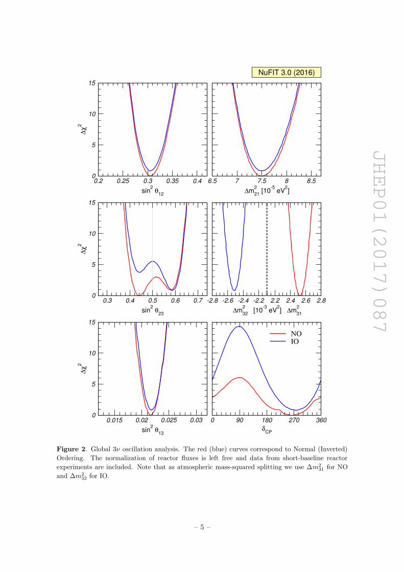
JHEP01(2017)087
0.2 0.25 0.3 0.35 0.4
sin2
θ12
0
5
10
15∆
χ2
6.5 7 7.5 8 8.5
∆m2
21 [10
-5 eV
2]
0.3 0.4 0.5 0.6 0.7
sin2
θ23
0
5
10
15
∆χ
2
-2.8 -2.6 -2.4 -2.2
∆m2
32 [10
-3 eV
2] ∆m
2
31
2.2 2.4 2.6 2.8
0.015 0.02 0.025 0.03
sin2
θ13
0
5
10
15
∆χ
2
0 90 180 270 360
δCP
NO
IO
NuFIT 3.0 (2016)
Figure 2. Global 3ν oscillation analysis. The red (blue) curves correspond to Normal (Inverted)
Ordering. The normalization of reactor fluxes is left free and data from short-baseline reactor
experiments are included. Note that as atmospheric mass-squared splitting we use ∆m231 for NO
and ∆m232 for IO.
– 5 –
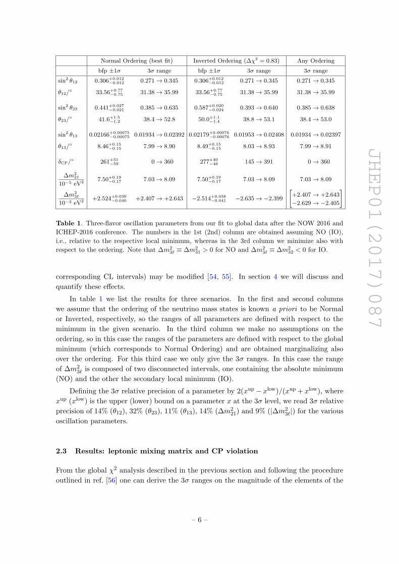
JHEP01(2017)087
Normal Ordering (best fit) Inverted Ordering (∆χ2 = 0.83) Any Ordering
bfp ±1σ 3σ range bfp ±1σ 3σ range 3σ range
sin2 θ12 0.306+0.012−0.012 0.271→ 0.345 0.306+0.012
−0.012 0.271→ 0.345 0.271→ 0.345
θ12/◦ 33.56+0.77
−0.75 31.38→ 35.99 33.56+0.77−0.75 31.38→ 35.99 31.38→ 35.99
sin2 θ23 0.441+0.027−0.021 0.385→ 0.635 0.587+0.020
−0.024 0.393→ 0.640 0.385→ 0.638
θ23/◦ 41.6+1.5
−1.2 38.4→ 52.8 50.0+1.1−1.4 38.8→ 53.1 38.4→ 53.0
sin2 θ13 0.02166+0.00075−0.00075 0.01934→ 0.02392 0.02179+0.00076
−0.00076 0.01953→ 0.02408 0.01934→ 0.02397
θ13/◦ 8.46+0.15
−0.15 7.99→ 8.90 8.49+0.15−0.15 8.03→ 8.93 7.99→ 8.91
δCP/◦ 261+51
−59 0→ 360 277+40−46 145→ 391 0→ 360
∆m221
10−5 eV2 7.50+0.19−0.17 7.03→ 8.09 7.50+0.19
−0.17 7.03→ 8.09 7.03→ 8.09
∆m23`
10−3 eV2 +2.524+0.039−0.040 +2.407→ +2.643 −2.514+0.038
−0.041 −2.635→ −2.399
[+2.407→ +2.643
−2.629→ −2.405
]
Table 1. Three-flavor oscillation parameters from our fit to global data after the NOW 2016 and
ICHEP-2016 conference. The numbers in the 1st (2nd) column are obtained assuming NO (IO),
i.e., relative to the respective local minimum, whereas in the 3rd column we minimize also with
respect to the ordering. Note that ∆m23` ≡ ∆m2
31 > 0 for NO and ∆m23` ≡ ∆m2
32 < 0 for IO.
corresponding CL intervals) may be modified [54, 55]. In section 4 we will discuss and
quantify these effects.
In table 1 we list the results for three scenarios. In the first and second columns
we assume that the ordering of the neutrino mass states is known a priori to be Normal
or Inverted, respectively, so the ranges of all parameters are defined with respect to the
minimum in the given scenario. In the third column we make no assumptions on the
ordering, so in this case the ranges of the parameters are defined with respect to the global
minimum (which corresponds to Normal Ordering) and are obtained marginalizing also
over the ordering. For this third case we only give the 3σ ranges. In this case the range
of ∆m23` is composed of two disconnected intervals, one containing the absolute minimum
(NO) and the other the secondary local minimum (IO).
Defining the 3σ relative precision of a parameter by 2(xup − xlow)/(xup + xlow), where
xup (xlow) is the upper (lower) bound on a parameter x at the 3σ level, we read 3σ relative
precision of 14% (θ12), 32% (θ23), 11% (θ13), 14% (∆m221) and 9% (|∆m2
3`|) for the various
oscillation parameters.
2.3 Results: leptonic mixing matrix and CP violation
From the global χ2 analysis described in the previous section and following the procedure
outlined in ref. [56] one can derive the 3σ ranges on the magnitude of the elements of the
– 6 –

JHEP01(2017)087
0.025 0.03 0.035 0.04
JCP
max = c
12 s
12 c
23 s
23 c
2
13 s
13
0
5
10
15∆
χ2
-0.04 -0.02 0 0.02 0.04
JCP
= JCP
max sinδ
CP
NO
IO
NuFIT 3.0 (2016)
Figure 3. Dependence of the global ∆χ2 function on the Jarlskog invariant. The red (blue) curves
are for NO (IO).
leptonic mixing matrix:
|U | =
0.800→ 0.844 0.515→ 0.581 0.139→ 0.155
0.229→ 0.516 0.438→ 0.699 0.614→ 0.790
0.249→ 0.528 0.462→ 0.715 0.595→ 0.776
. (2.1)
Note that there are strong correlations between the elements due to the unitary constraint.
The present status of the determination of leptonic CP violation is illustrated in fig-
ure 3. In the left panel we show the dependence of ∆χ2 of the global analysis on the Jarlskog
invariant which gives a convention-independent measure of CP violation [57], defined as
usual by:
Im[UαiU
∗αjU
∗βiUβj
]≡ Jmax
CP sin δ = cos θ12 sin θ12 cos θ23 sin θ23 cos2 θ13 sin θ13 sin δ (2.2)
where we have used the parametrization in eq. (1.1). Thus the determination of the mixing
angles yields at present a maximum allowed CP violation
JmaxCP = 0.0329± 0.0007 (+0.0021
−0.0024) (2.3)
at 1σ (3σ) for both orderings. The preference of the present data for non-zero δCP implies
a best fit value JbestCP = −0.033, which is favored over CP conservation with ∆χ2 = 1.7.
These numbers can be compared with the size of the Jarlskog invariant in the quark sector,
which is determined to be JquarksCP = (3.04+0.21
−0.20)× 10−5 [58].
In figure 4 we recast the allowed regions for the leptonic mixing matrix in terms of
one leptonic unitarity triangle. Since in the analysis U is unitary by construction, any
given pair of rows or columns can be used to define a triangle in the complex plane.
In the figure we show the triangle corresponding to the unitarity conditions on the first
and third columns which is the equivalent to the one usually shown for the quark sector.
– 7 –
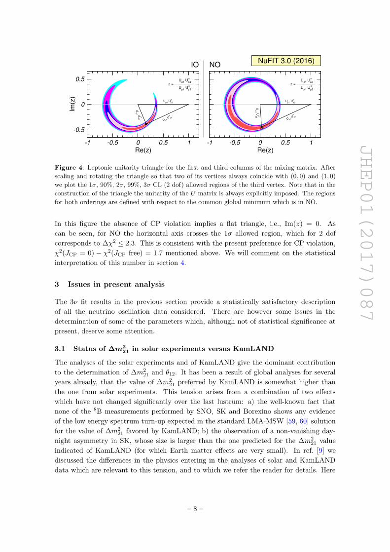
JHEP01(2017)087
-1 -0.5 0 0.5 1
Re(z)
-0.5
0
0.5
Im(z
)
z = −
Ue1
U∗e3
Uµ1
U∗µ3
Ue1 U
∗e3
Uµ1
U∗µ3
U τ1 U
∗τ3
★
-1 -0.5 0 0.5 1
Re(z)
z = −
Ue1
U∗e3
Uµ1
U∗µ3
Uµ1
U∗µ3
U τ1 U
∗τ3
Ue1 U
∗e3
NuFIT 3.0 (2016)NOIO
Figure 4. Leptonic unitarity triangle for the first and third columns of the mixing matrix. After
scaling and rotating the triangle so that two of its vertices always coincide with (0, 0) and (1, 0)
we plot the 1σ, 90%, 2σ, 99%, 3σ CL (2 dof) allowed regions of the third vertex. Note that in the
construction of the triangle the unitarity of the U matrix is always explicitly imposed. The regions
for both orderings are defined with respect to the common global minimum which is in NO.
In this figure the absence of CP violation implies a flat triangle, i.e., Im(z) = 0. As
can be seen, for NO the horizontal axis crosses the 1σ allowed region, which for 2 dof
corresponds to ∆χ2 ≤ 2.3. This is consistent with the present preference for CP violation,
χ2(JCP = 0) − χ2(JCP free) = 1.7 mentioned above. We will comment on the statistical
interpretation of this number in section 4.
3 Issues in present analysis
The 3ν fit results in the previous section provide a statistically satisfactory description
of all the neutrino oscillation data considered. There are however some issues in the
determination of some of the parameters which, although not of statistical significance at
present, deserve some attention.
3.1 Status of ∆m221 in solar experiments versus KamLAND
The analyses of the solar experiments and of KamLAND give the dominant contribution
to the determination of ∆m221 and θ12. It has been a result of global analyses for several
years already, that the value of ∆m221 preferred by KamLAND is somewhat higher than
the one from solar experiments. This tension arises from a combination of two effects
which have not changed significantly over the last lustrum: a) the well-known fact that
none of the 8B measurements performed by SNO, SK and Borexino shows any evidence
of the low energy spectrum turn-up expected in the standard LMA-MSW [59, 60] solution
for the value of ∆m221 favored by KamLAND; b) the observation of a non-vanishing day-
night asymmetry in SK, whose size is larger than the one predicted for the ∆m221 value
indicated of KamLAND (for which Earth matter effects are very small). In ref. [9] we
discussed the differences in the physics entering in the analyses of solar and KamLAND
data which are relevant to this tension, and to which we refer the reader for details. Here
– 8 –

JHEP01(2017)087
★
★
0.2 0.25 0.3 0.35 0.4
sin2θ
12
0
2
4
6
8
10
12
14∆
m2 2
1 [10
−5 e
V2]
θ13
= 8.5°
2 4 6 8 10
∆m2
21 [10
−5 eV
2]
0
2
4
6
8
10
12
∆χ
2
GS98
AGSS09KamLAND
NuFIT 3.0 (2016)
Figure 5. Left: allowed parameter regions (at 1σ, 90%, 2σ, 99% and 3σ CL for 2 dof) from the
combined analysis of solar data for GS98 model (full regions with best fit marked by black star) and
AGSS09 model (dashed void contours with best fit marked by a white dot), and for the analysis of
KamLAND data (solid green contours with best fit marked by a green star) for fixed θ13 = 8.5◦.
Right: ∆χ2 dependence on ∆m221 for the same three analyses after marginalizing over θ12.
for sake of completeness we show in figure 5 the quantification of this tension in our present
global analysis. As seen in the figure, the best fit value of ∆m221 of KamLAND lays at the
boundary of the 2σ allowed range of the solar neutrino analysis.
Also for illustration of the independence of these results with respect to the solar
modeling, the solar neutrino regions are shown for two latest versions of the Standard
Solar Model, namely the GS98 and the AGSS09 models [61] obtained with two different
determinations of the solar abundances [62].
3.2 ∆m23` determination in LBL accelerator experiments versus reactors
Figure 6 illustrates the contribution to the present determination of ∆m23` from the different
data sets. In the left panels we focus on the determination from long baseline experiments,
which is mainly from νµ disappearance data. We plot the 1σ and 2σ allowed regions (2 dof)
in the dominant parameters ∆m23` and θ23. As seen in the figure, although the agreement
between the different experiments is reasonable, some “tension” starts to appear in the
determination of both parameters among the LBL accelerator experiments. In particular
we see that the recent results from NOνA, unlike those from T2K, favor a non-maximal
value of θ23. It is important to notice that in the context of 3ν mixing the relevant oscillation
probabilities for the LBL accelerator experiments also depend on θ13 (and on the θ12 and
∆m221 parameters which are independently well constrained by solar and KamLAND data).
To construct the regions plotted in the left panels of figure 6, we adopt the procedure
– 9 –
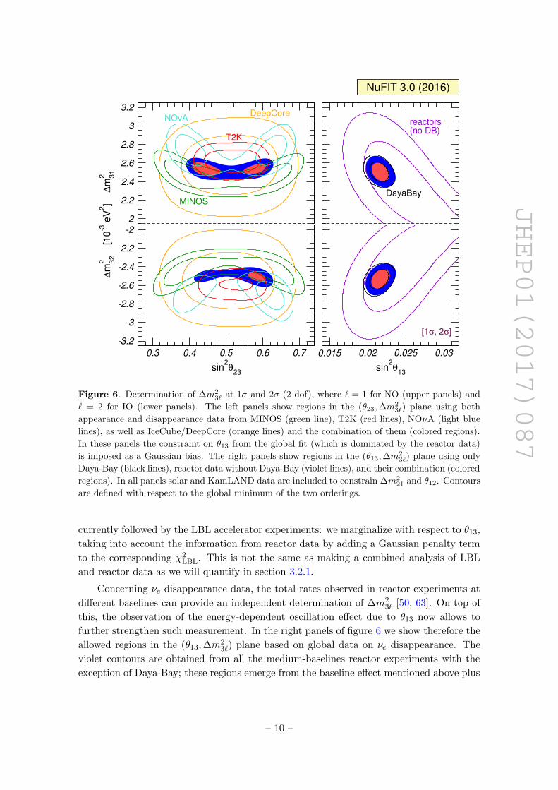
JHEP01(2017)087
2
2.2
2.4
2.6
2.8
3
3.2∆
m2 3
2 [1
0-3
eV
2] ∆
m2 3
1NOvA
T2K
MINOS
DeepCore
0.3 0.4 0.5 0.6 0.7
sin2θ
23
-3.2
-3
-2.8
-2.6
-2.4
-2.2
-2
reactors(no DB)
DayaBay
0.015 0.02 0.025 0.03
sin2θ
13
[1σ, 2σ]
NuFIT 3.0 (2016)
Figure 6. Determination of ∆m23` at 1σ and 2σ (2 dof), where ` = 1 for NO (upper panels) and
` = 2 for IO (lower panels). The left panels show regions in the (θ23,∆m23`) plane using both
appearance and disappearance data from MINOS (green line), T2K (red lines), NOνA (light blue
lines), as well as IceCube/DeepCore (orange lines) and the combination of them (colored regions).
In these panels the constraint on θ13 from the global fit (which is dominated by the reactor data)
is imposed as a Gaussian bias. The right panels show regions in the (θ13,∆m23`) plane using only
Daya-Bay (black lines), reactor data without Daya-Bay (violet lines), and their combination (colored
regions). In all panels solar and KamLAND data are included to constrain ∆m221 and θ12. Contours
are defined with respect to the global minimum of the two orderings.
currently followed by the LBL accelerator experiments: we marginalize with respect to θ13,
taking into account the information from reactor data by adding a Gaussian penalty term
to the corresponding χ2LBL. This is not the same as making a combined analysis of LBL
and reactor data as we will quantify in section 3.2.1.
Concerning νe disappearance data, the total rates observed in reactor experiments at
different baselines can provide an independent determination of ∆m23` [50, 63]. On top of
this, the observation of the energy-dependent oscillation effect due to θ13 now allows to
further strengthen such measurement. In the right panels of figure 6 we show therefore the
allowed regions in the (θ13,∆m23`) plane based on global data on νe disappearance. The
violet contours are obtained from all the medium-baselines reactor experiments with the
exception of Daya-Bay; these regions emerge from the baseline effect mentioned above plus
– 10 –
JHEP01(2017)087
spectral information from Double-Chooz.3 The black contours are based on the energy
spectrum in Daya-Bay, whereas the colored regions show the combination.
By comparing the left and right panels of figure 6 we observe that the combined νµ and
νe disappearance experiments provide a consistent determination of |∆m23`| with similar
precision. However when comparing the region for each LBL experiment with that of the
reactor experiments we find some dispersion in the best fit values and allowed ranges. This
is more clearly illustrated in the upper panels of figure 7, where we plot the one dimensional
projection of the regions in figure 6 as a function of ∆m23` after marginalization over θ23 for
each of the LBL experiments and for their combination, together with that from reactor
data after marginalization over θ13. The projections are shown for NO(right) and IO(left).
Let us stress that the curves corresponding to LBL experiments in the upper panels of
figure 7 (as well as those in the upper panels of figures 8 and 9) have been obtained by a
partial combination of the information on the shown parameter (∆m23` or θ23 or δCP) from
LBL with that of θ13 from reactors, because in these plots only the θ13 constraint from
reactors is imposed while the dependence on ∆m23` is neglected. This corresponds to the
1-dim projections of the function:
∆χ2LBL+θREA
13(θ23, δCP,∆m
23`)
= minθ13
[χ2
LBL(θ13, θ23, δCP,∆m23`) + min
∆m23`
χ2REA(θ13,∆m
23`)]− χ2
min . (3.1)
However, since reactor data also depends on ∆m23` the full combination of reactor and
LBL results implies that one must add consistently the χ2 functions of the LBL experiment
with that of reactors evaluated the same value of ∆m23`, this is
∆χ2LBL+REA(θ23, δCP,∆m
23`)
= minθ13
[χ2
LBL(θ13, θ23, δCP,∆m23`) + χ2
REA(θ13,∆m23`)]− χ2
min . (3.2)
We discuss next the effect of combining consistently the information from LBL and reactor
experiments in the present determination of θ23, δCP and the ordering.
3.2.1 Impact on the determination of θ23, mass ordering, and δCP
We plot in the lower panels of figures 7–9 the one dimensional projections of ∆χ2LBL+REA for
each of the parameters θ23, δCP, ∆m23` (marginalized with respect to the two undisplayed
parameters) for the consistent LBL+REA combinations with both the information on θ13
and ∆m23` from reactors included, eq. (3.2). As mentioned before, the curves in the upper
panels for these figures show the corresponding 1-dimensional projections for the partial
combination, in which only the θ13 constraint from reactors is used, eq. (3.1). For each
experiment the curves in these figures are defined with respect to the global minimum of
the two orderings, so the relative height of the minimum in one ordering vs the other gives
a measure of the ordering favored by each of the experiments.
3Recently, RENO has presented a spectral analysis based on an exposure of 500 days [64]. Here we prefer
to include from RENO only the total rate measurement, based on the larger exposure of 800 days [37].
– 11 –
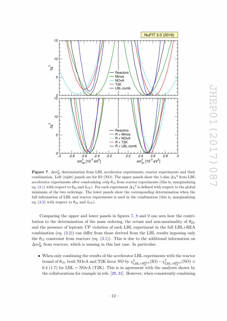
JHEP01(2017)087
0
5
10
15
∆χ
2
ReactorsMinosNOvAT2KLBL-comb
-3 -2.8 -2.6 -2.4 -2.2
∆m2
32 [10
-3 eV
2]
0
5
10
15
∆χ
2
2.2 2.4 2.6 2.8 3
∆m2
31 [10
-3 eV
2]
ReactorsR + MinosR + NOvAR + T2KR + LBL-comb
NuFIT 3.0 (2016)
Figure 7. ∆m23` determination from LBL accelerator experiments, reactor experiments and their
combination. Left (right) panels are for IO (NO). The upper panels show the 1-dim ∆χ2 from LBL
accelerator experiments after constraining only θ13 from reactor experiments (this is, marginalizing
eq. (3.1) with respect to θ23 and δCP). For each experiment ∆χ2 is defined with respect to the global
minimum of the two orderings. The lower panels show the corresponding determination when the
full information of LBL and reactor experiments is used in the combination (this is, marginalizing
eq. (3.2) with respect to θ23 and δCP).
Comparing the upper and lower panels in figures 7, 8 and 9 one sees how the contri-
bution to the determination of the mass ordering, the octant and non-maximality of θ23,
and the presence of leptonic CP violation of each LBL experiment in the full LBL+REA
combination (eq. (3.2)) can differ from those derived from the LBL results imposing only
the θ13 constraint from reactors (eq. (3.1)). This is due to the additional information on
∆m23` from reactors, which is missing in this last case. In particular:
• When only combining the results of the accelerator LBL experiments with the reactor
bound of θ13, both NOνA and T2K favor NO by χ2LBL+θREA
13(IO)−χ2
LBL+θREA13
(NO) '0.4 (1.7) for LBL = NOνA (T2K). This is in agreement with the analyses shown by
the collaborations for example in refs. [29, 31]. However, when consistently combining
– 12 –
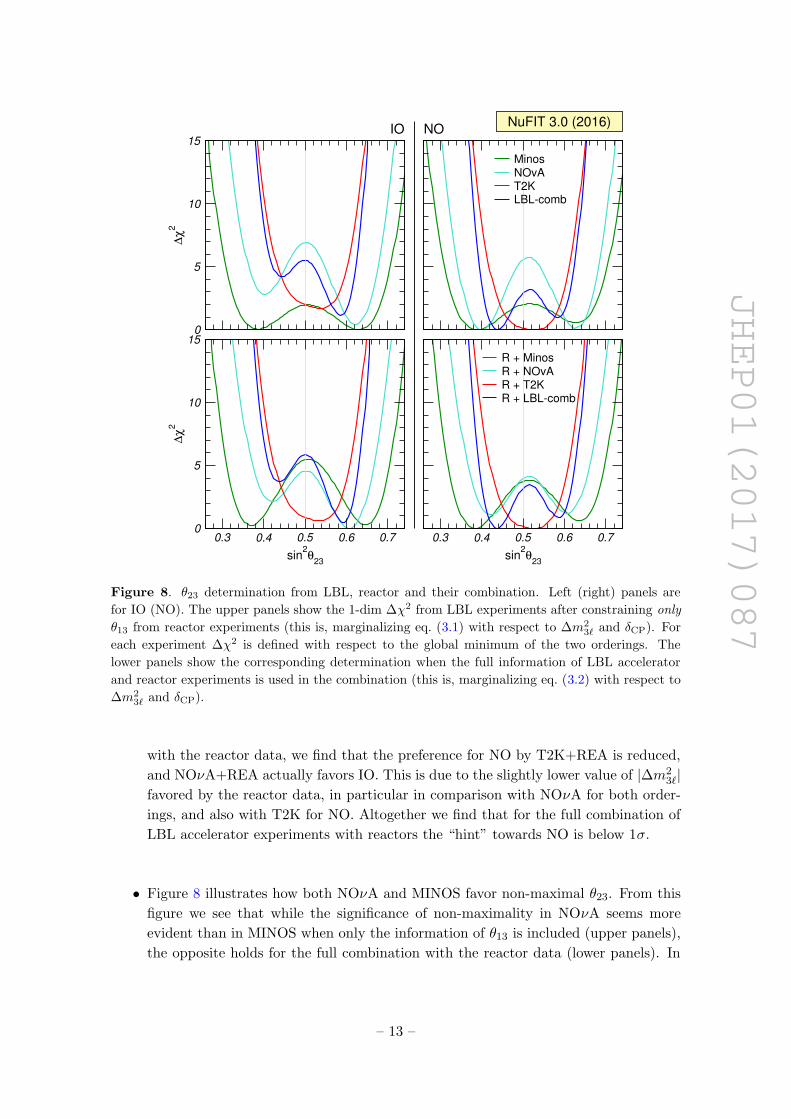
JHEP01(2017)087
0
5
10
15
∆χ
2MinosNOvAT2KLBL-comb
0.3 0.4 0.5 0.6 0.7
sin2θ
23
0
5
10
15
∆χ
2
0.3 0.4 0.5 0.6 0.7
sin2θ
23
R + MinosR + NOvAR + T2KR + LBL-comb
NuFIT 3.0 (2016)IO NO
Figure 8. θ23 determination from LBL, reactor and their combination. Left (right) panels are
for IO (NO). The upper panels show the 1-dim ∆χ2 from LBL experiments after constraining only
θ13 from reactor experiments (this is, marginalizing eq. (3.1) with respect to ∆m23` and δCP). For
each experiment ∆χ2 is defined with respect to the global minimum of the two orderings. The
lower panels show the corresponding determination when the full information of LBL accelerator
and reactor experiments is used in the combination (this is, marginalizing eq. (3.2) with respect to
∆m23` and δCP).
with the reactor data, we find that the preference for NO by T2K+REA is reduced,
and NOνA+REA actually favors IO. This is due to the slightly lower value of |∆m23`|
favored by the reactor data, in particular in comparison with NOνA for both order-
ings, and also with T2K for NO. Altogether we find that for the full combination of
LBL accelerator experiments with reactors the “hint” towards NO is below 1σ.
• Figure 8 illustrates how both NOνA and MINOS favor non-maximal θ23. From this
figure we see that while the significance of non-maximality in NOνA seems more
evident than in MINOS when only the information of θ13 is included (upper panels),
the opposite holds for the full combination with the reactor data (lower panels). In
– 13 –
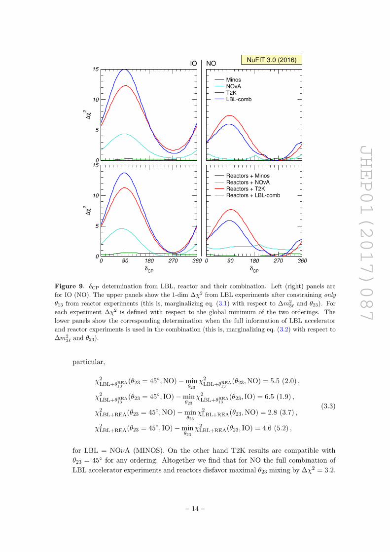
JHEP01(2017)087
0
5
10
15
∆χ
2MinosNOvAT2KLBL-comb
0 90 180 270 360
δCP
0
5
10
15
∆χ
2
0 90 180 270 360
δCP
Reactors + MinosReactors + NOvAReactors + T2KReactors + LBL-comb
NuFIT 3.0 (2016)IO NO
Figure 9. δCP determination from LBL, reactor and their combination. Left (right) panels are
for IO (NO). The upper panels show the 1-dim ∆χ2 from LBL experiments after constraining only
θ13 from reactor experiments (this is, marginalizing eq. (3.1) with respect to ∆m23` and θ23). For
each experiment ∆χ2 is defined with respect to the global minimum of the two orderings. The
lower panels show the corresponding determination when the full information of LBL accelerator
and reactor experiments is used in the combination (this is, marginalizing eq. (3.2) with respect to
∆m23` and θ23).
particular,
χ2LBL+θREA
13(θ23 = 45◦,NO)−min
θ23χ2
LBL+θREA13
(θ23,NO) = 5.5 (2.0) ,
χ2LBL+θREA
13(θ23 = 45◦, IO)−min
θ23χ2
LBL+θREA13
(θ23, IO) = 6.5 (1.9) ,
χ2LBL+REA(θ23 = 45◦,NO)−min
θ23χ2
LBL+REA(θ23,NO) = 2.8 (3.7) ,
χ2LBL+REA(θ23 = 45◦, IO)−min
θ23χ2
LBL+REA(θ23, IO) = 4.6 (5.2) ,
(3.3)
for LBL = NOνA (MINOS). On the other hand T2K results are compatible with
θ23 = 45◦ for any ordering. Altogether we find that for NO the full combination of
LBL accelerator experiments and reactors disfavor maximal θ23 mixing by ∆χ2 = 3.2.
– 14 –

JHEP01(2017)087
• Regarding the octant of θ23, for IO all LBL accelerator experiments are better de-
scribed with θ23 > 45◦, adding up to a ∼ 1.8σ preference for that octant. Conversely,
for NO θ23 < 45◦ is favored at ∼ 1σ.
• From figure 9 we see that the “hint” for a CP phase around 270◦ is mostly driven
by T2K data, with some extra contribution from NOνA in the case of IO. Within
the present precision the favored ranges of δCP in each ordering by the combination
of LBL accelerator experiments are pretty independent on the inclusion of the ∆m23`
information from reactors.
3.3 Analysis of Super-Kamiokande atmospheric data
In all the results discussed so far we have not included information from Super-Kamiokande
atmospheric data. The reason is that our oscillation analysis cannot reproduce that of the
collaboration presented in their talks in the last two years (see for example ref. [66] for
their latest unpublished results).
Already since SK2 the Super-Kamiokande collaboration has been presenting its ex-
perimental results in terms of a growing number of data samples. The rates for some of
those samples cannot be predicted (and therefore included in a statistical analysis) with-
out a detailed simulation of the detector, which can only be made by the experimental
collaboration itself. Our analysis of Super-Kamiokande data has been always based on the
“classical” set of samples for which our simulations were reliable enough: sub-GeV and
multi-GeV e-like and µ-like fully contained events, as well as partially contained, stopping
and through-going muon data, each divided into 10 angular bins for a total of 70 energy and
zenith angle bins (details on our simulation of the data samples and the statistical analysis
are given in the appendix of ref. [3]). Despite the limitations, until recently our results
represented the most up-to-date analysis of the atmospheric neutrino data which could
be performed outside the collaboration, and we were able to reproduce with reasonable
precision the oscillation results of the full analysis presented by SK – both for what con-
cerns the determination of the dominant parameters ∆m23` and θ23, as well as their rather
marginal sensitivity to the subdominant νe appearance effects driven by θ13 (and conse-
quently to δCP and the ordering). Thus we confidently included our own implementation
of the Super-Kamiokande χ2 in our global fit.
However, in the last two years Super-Kamiokande has developed a new analysis method
in which a set of neural network based selections are introduced, some of them with the aim
of constructing νe+νe enriched samples which are then further classified into νe-like and νe-
like subsamples, thus increasing the sensitivity to subleading parameters such as the mass
ordering and δCP [65, 67]. The selection criteria are constructed to exploit the expected
differences in the number of charged pions and transverse momentum in the interaction
of νe versus νe. With this new analysis method Super-Kamiokande has been reporting in
talks an increasing sensitivity to the ordering and to δCP: for example, the preliminary
results of the analysis of SK1–4 (including 2520 days of SK4) [66] in combination with the
reactor constraint of θ13 show a preference for NO with a ∆χ2(IO) = 4.3 and variation of
χ2(δCP) with the CP phase at the level of ∼ 1.7σ.
– 15 –
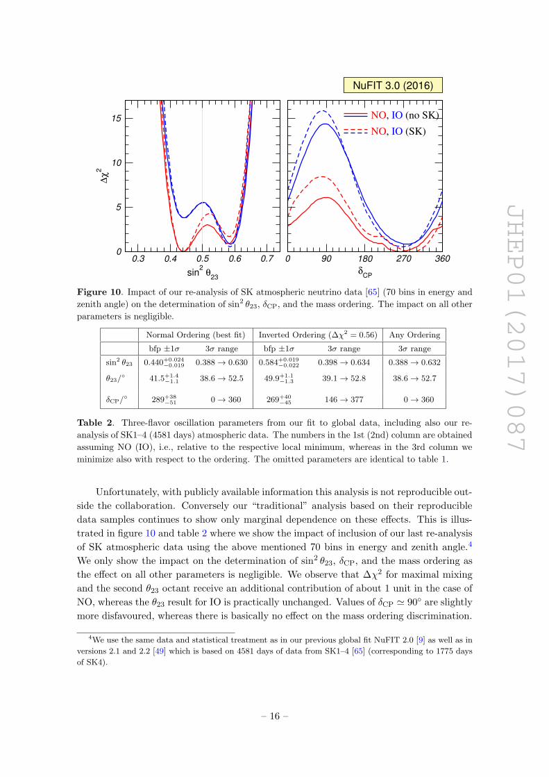
JHEP01(2017)087
0.3 0.4 0.5 0.6 0.7
sin2
θ23
0
5
10
15
∆χ
2
0 90 180 270 360
δCP
NO, IO (no SK)
NO, IO (SK)
NuFIT 3.0 (2016)
Figure 10. Impact of our re-analysis of SK atmospheric neutrino data [65] (70 bins in energy and
zenith angle) on the determination of sin2 θ23, δCP, and the mass ordering. The impact on all other
parameters is negligible.
Normal Ordering (best fit) Inverted Ordering (∆χ2 = 0.56) Any Ordering
bfp ±1σ 3σ range bfp ±1σ 3σ range 3σ range
sin2 θ23 0.440+0.024−0.019 0.388→ 0.630 0.584+0.019
−0.022 0.398→ 0.634 0.388→ 0.632
θ23/◦ 41.5+1.4
−1.1 38.6→ 52.5 49.9+1.1−1.3 39.1→ 52.8 38.6→ 52.7
δCP/◦ 289+38
−51 0→ 360 269+40−45 146→ 377 0→ 360
Table 2. Three-flavor oscillation parameters from our fit to global data, including also our re-
analysis of SK1–4 (4581 days) atmospheric data. The numbers in the 1st (2nd) column are obtained
assuming NO (IO), i.e., relative to the respective local minimum, whereas in the 3rd column we
minimize also with respect to the ordering. The omitted parameters are identical to table 1.
Unfortunately, with publicly available information this analysis is not reproducible out-
side the collaboration. Conversely our “traditional” analysis based on their reproducible
data samples continues to show only marginal dependence on these effects. This is illus-
trated in figure 10 and table 2 where we show the impact of inclusion of our last re-analysis
of SK atmospheric data using the above mentioned 70 bins in energy and zenith angle.4
We only show the impact on the determination of sin2 θ23, δCP, and the mass ordering as
the effect on all other parameters is negligible. We observe that ∆χ2 for maximal mixing
and the second θ23 octant receive an additional contribution of about 1 unit in the case of
NO, whereas the θ23 result for IO is practically unchanged. Values of δCP ' 90◦ are slightly
more disfavoured, whereas there is basically no effect on the mass ordering discrimination.
4We use the same data and statistical treatment as in our previous global fit NuFIT 2.0 [9] as well as in
versions 2.1 and 2.2 [49] which is based on 4581 days of data from SK1–4 [65] (corresponding to 1775 days
of SK4).
– 16 –

JHEP01(2017)087
In summary, with the information at hand we are not able to reproduce the elements
driving the main dependence on the subdominant effects of the official (though preliminary
and unpublished) Super-Kamiokande results, while the dominant parameters are currently
well determined by LBL experiments. For these reasons we have decided not to include our
re-analysis of Super-Kamiokande data in our preferred global fit presented in the previous
section. Needless to say that when enough quantitative information becomes available to
allow a reliable simulation of the subdominant νe-driven effects, we will proceed to include
it in our global analysis.
4 Monte Carlo evaluation of confidence levels for θ23, δCP and ordering
At present the three least known neutrino oscillation parameters are the Dirac CP violating
phase δCP, the octant of θ23 and the mass ordering (which in what follows we will denote
by “O”). In order to study the information from data on these parameters one can use two
∆χ2 test statistics [55, 68]:
∆χ2 (δCP,O) = minx1
χ2 (δCP,O, x1)− χ2min , (4.1)
∆χ2 (θ23,O) = minx2
χ2 (θ23,O, x2)− χ2min , (4.2)
where the minimization in the first equation is performed with respect to all oscillation
parameters except δCP and the ordering (x1 = {θ12, θ13, θ23,∆m221, |∆m2
3`|}), while in the
second equation the minimization is over all oscillation parameters except θ23 and the
ordering (x2 = {θ12, θ13, δCP,∆m221, |∆m2
3`|}). Here χ2min indicates the χ2 minimum with
respect to all oscillation parameters including the mass ordering.
We have plotted the values of these test statistics in the lower right and central left
panels in figure 2. We can use them not only for the determination of δCP and θ23,
respectively, but also of the mass ordering. For instance, using eq. (4.1) we can determine
a confidence interval for δCP at a given CL for both orderings. However, below a certain
CL no interval will appear for the less favored ordering. In this sense we can exclude that
ordering at the CL at which the corresponding interval for δCP disappears. Note that a
similar prescription to test the mass ordering can be built for any other parameter as well,
e.g., for θ23 using eq. (4.2).5
In section 2 we have presented confidence intervals assuming that the test statistics
follow a χ2-distribution with 1 dof, relying on Wilks theorem to hold [70] (this is what we
call the Gaussian limit). However, the test statistics in eqs. (4.1) and (4.2) are expected
not to follow Wilks’ theorem because of several reasons [68]:
• Sensitivity of current data to δCP is still limited, as can be seen in figure 2: all values
of δCP have ∆χ2 < 14, and for NO not even ∆χ2 = 6 is attained.
• Regarding θ23, its precision is dominated by νµ disappearance experiments. Since
the relevant survival probability depends dominantly on sin2 2θ23, there is both a
5Let us mention that this method to determine the mass ordering is different from the one based on the
test statistics T discussed in ref. [69].
– 17 –
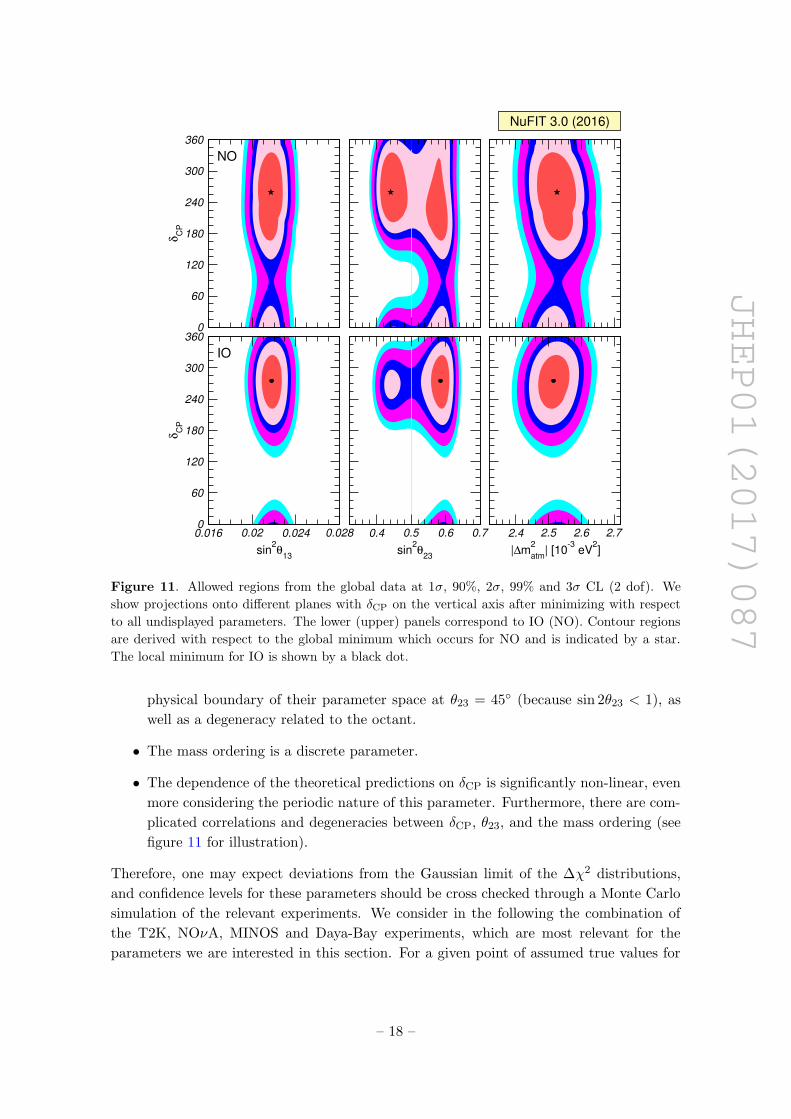
JHEP01(2017)087
★
0
60
120
180
240
300
360
δC
P
NO
★ ★
0.016 0.02 0.024 0.028
sin2θ
13
0
60
120
180
240
300
360
δC
P
IO
0.4 0.5 0.6 0.7
sin2θ
23
2.4 2.5 2.6 2.7
|∆m2
atm| [10
-3 eV
2]
NuFIT 3.0 (2016)
Figure 11. Allowed regions from the global data at 1σ, 90%, 2σ, 99% and 3σ CL (2 dof). We
show projections onto different planes with δCP on the vertical axis after minimizing with respect
to all undisplayed parameters. The lower (upper) panels correspond to IO (NO). Contour regions
are derived with respect to the global minimum which occurs for NO and is indicated by a star.
The local minimum for IO is shown by a black dot.
physical boundary of their parameter space at θ23 = 45◦ (because sin 2θ23 < 1), as
well as a degeneracy related to the octant.
• The mass ordering is a discrete parameter.
• The dependence of the theoretical predictions on δCP is significantly non-linear, even
more considering the periodic nature of this parameter. Furthermore, there are com-
plicated correlations and degeneracies between δCP, θ23, and the mass ordering (see
figure 11 for illustration).
Therefore, one may expect deviations from the Gaussian limit of the ∆χ2 distributions,
and confidence levels for these parameters should be cross checked through a Monte Carlo
simulation of the relevant experiments. We consider in the following the combination of
the T2K, NOνA, MINOS and Daya-Bay experiments, which are most relevant for the
parameters we are interested in this section. For a given point of assumed true values for
– 18 –
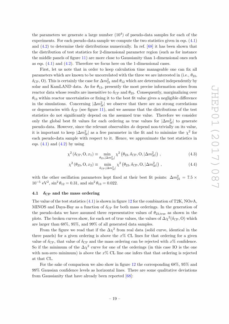
JHEP01(2017)087
the parameters we generate a large number (104) of pseudo-data samples for each of the
experiments. For each pseudo-data sample we compute the two statistics given in eqs. (4.1)
and (4.2) to determine their distributions numerically. In ref. [68] it has been shown that
the distribution of test statistics for 2-dimensional parameter region (such as for instance
the middle panels of figure 11) are more close to Gaussianity than 1-dimensional ones such
as eqs. (4.1) and (4.2). Therefore we focus here on the 1-dimensional cases.
First, let us note that in order to keep calculation time manageable one can fix all
parameters which are known to be uncorrelated with the three we are interested in (i.e., θ23,
δCP, O). This is certainly the case for ∆m221 and θ12 which are determined independently by
solar and KamLAND data. As for θ13, presently the most precise information arises from
reactor data whose results are insensitive to δCP and θ23. Consequently, marginalizing over
θ13 within reactor uncertainties or fixing it to the best fit value gives a negligible difference
in the simulations. Concerning |∆m23`| we observe that there are no strong correlations
or degeneracies with δCP (see figure 11), and we assume that the distributions of the test
statistics do not significantly depend on the assumed true value. Therefore we consider
only the global best fit values for each ordering as true values for |∆m23`| to generate
pseudo-data. However, since the relevant observables do depend non-trivially on its value,
it is important to keep |∆m23`| as a free parameter in the fit and to minimize the χ2 for
each pseudo-data sample with respect to it. Hence, we approximate the test statistics in
eqs. (4.1) and (4.2) by using
χ2 (δCP,O, x1) ≡ minθ23,|∆m2
3`|χ2(θ23, δCP,O, |∆m2
3`|), (4.3)
χ2 (θ23,O, x2) ≡ minδCP,|∆m2
3`|χ2(θ23, δCP,O, |∆m2
3`|), (4.4)
with the other oscillation parameters kept fixed at their best fit points: ∆m221 = 7.5 ×
10−5 eV2, sin2 θ12 = 0.31, and sin2 θ13 = 0.022.
4.1 δCP and the mass ordering
The value of the test statistics (4.1) is shown in figure 12 for the combination of T2K, NOνA,
MINOS and Daya-Bay as a function of δCP for both mass orderings. In the generation of
the pseudo-data we have assumed three representative values of θ23,true as shown in the
plots. The broken curves show, for each set of true values, the values of ∆χ2(δCP,O) which
are larger than 68%, 95%, and 99% of all generated data samples.
From the figure we read that if the ∆χ2 from real data (solid curve, identical in the
three panels) for a given ordering is above the x% CL lines for that ordering for a given
value of δCP, that value of δCP and the mass ordering can be rejected with x% confidence.
So if the minimum of the ∆χ2 curve for one of the orderings (in this case IO is the one
with non-zero minimum) is above the x% CL line one infers that that ordering is rejected
at that CL.
For the sake of comparison we also show in figure 12 the corresponding 68%, 95% and
99% Gaussian confidence levels as horizontal lines. There are some qualitative deviations
from Gaussianity that have already been reported [68]:
– 19 –

JHEP01(2017)087
0 90 180 270
δCP
0
2
4
6
8
10
12
14
∆χ
2
sin2θ
23 = 0.44
0 90 180 270
δCP
sin2θ
23 = 0.53
0 90 180 270 360
δCP
sin2θ
23 = 0.60
NOIO
NuFIT 3.0 (2016)
Figure 12. 68%, 95% and 99% confidence levels (broken curves) for the test statistics (4.1) along
with its value (solid curves) for the combination of T2K, NOνA, MINOS and reactor data. The value
of sin2 θ23 given in each panel corresponds to the assumed true value chosen to generate the pseudo-
experiments and for all panels we take ∆m23`,true = −2.53× 10⁻³ eV2 for IO and +2.54× 10⁻³ eV2
for NO. The solid horizontal lines represent the 68%, 95% and 99% CL predictions from Wilks’
theorem.
• For θ23 < 45◦, δCP = 90◦, and IO as well as for θ23 > 45◦, δCP = 270◦ and NO,
the confidence levels decrease. This effect arises because at those points in parameter
space the νµ → νe oscillation probability has a minimum or a maximum, respectively.
Therefore, statistical fluctuations leading to less (or more) events than predicted
cannot be accommodated by adjusting the parameters. ∆χ2 is small more often
and the confidence levels decrease. This is an effect always present at boundaries in
parameter space, usually referred to as an effective decrease in the number of degrees
of freedom in the model.
• Conversely for δCP ∼ 90◦ for θ23 > 45◦, and δCP ∼ 270◦ for θ23 < 45◦, the confidence
levels increase. This is associated with the prominent presence of the octant degen-
eracy. Degeneracies imply that statistical fluctuations can drive you away from the
true value, ∆χ2 increases, and the confidence levels increase. This is usually referred
to as an effective increase in the number of degrees of freedom in the model due to
degeneracies.
• Overall we find that with present data confidence levels are clearly closer to Gaus-
sianity than found in refs. [9, 68], where similar simulations have been performed
with less data available. For those data sets confidence levels were consistently below
their Gaussian limit. This was mainly a consequence of the limited statistics and the
cyclic nature of δCP which lead to an effective decrease in the number of degrees of
– 20 –
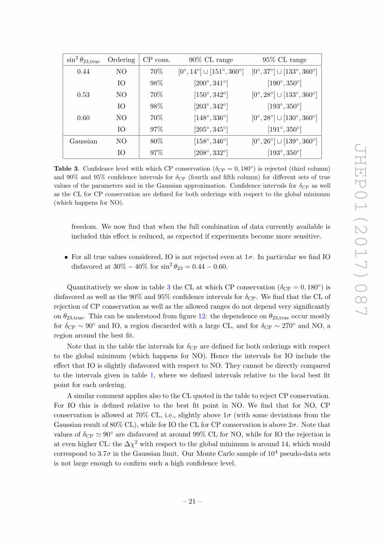
JHEP01(2017)087
sin2 θ23,true Ordering CP cons. 90% CL range 95% CL range
0.44 NO 70% [0◦, 14◦] ∪ [151◦, 360◦] [0◦, 37◦] ∪ [133◦, 360◦]
IO 98% [200◦, 341◦] [190◦, 350◦]
0.53 NO 70% [150◦, 342◦] [0◦, 28◦] ∪ [133◦, 360◦]
IO 98% [203◦, 342◦] [193◦, 350◦]
0.60 NO 70% [148◦, 336◦] [0◦, 28◦] ∪ [130◦, 360◦]
IO 97% [205◦, 345◦] [191◦, 350◦]
Gaussian NO 80% [158◦, 346◦] [0◦, 26◦] ∪ [139◦, 360◦]
IO 97% [208◦, 332◦] [193◦, 350◦]
Table 3. Confidence level with which CP conservation (δCP = 0, 180◦) is rejected (third column)
and 90% and 95% confidence intervals for δCP (fourth and fifth column) for different sets of true
values of the parameters and in the Gaussian approximation. Confidence intervals for δCP as well
as the CL for CP conservation are defined for both orderings with respect to the global minimum
(which happens for NO).
freedom. We now find that when the full combination of data currently available is
included this effect is reduced, as expected if experiments become more sensitive.
• For all true values considered, IO is not rejected even at 1σ. In particular we find IO
disfavored at 30%− 40% for sin2 θ23 = 0.44− 0.60.
Quantitatively we show in table 3 the CL at which CP conservation (δCP = 0, 180◦) is
disfavored as well as the 90% and 95% confidence intervals for δCP. We find that the CL of
rejection of CP conservation as well as the allowed ranges do not depend very significantly
on θ23,true. This can be understood from figure 12: the dependence on θ23,true occur mostly
for δCP ∼ 90◦ and IO, a region discarded with a large CL, and for δCP ∼ 270◦ and NO, a
region around the best fit.
Note that in the table the intervals for δCP are defined for both orderings with respect
to the global minimum (which happens for NO). Hence the intervals for IO include the
effect that IO is slightly disfavored with respect to NO. They cannot be directly compared
to the intervals given in table 1, where we defined intervals relative to the local best fit
point for each ordering.
A similar comment applies also to the CL quoted in the table to reject CP conservation.
For IO this is defined relative to the best fit point in NO. We find that for NO, CP
conservation is allowed at 70% CL, i.e., slightly above 1σ (with some deviations from the
Gaussian result of 80% CL), while for IO the CL for CP conservation is above 2σ. Note that
values of δCP ' 90◦ are disfavored at around 99% CL for NO, while for IO the rejection is
at even higher CL: the ∆χ2 with respect to the global minimum is around 14, which would
correspond to 3.7σ in the Gaussian limit. Our Monte Carlo sample of 104 pseudo-data sets
is not large enough to confirm such a high confidence level.
– 21 –
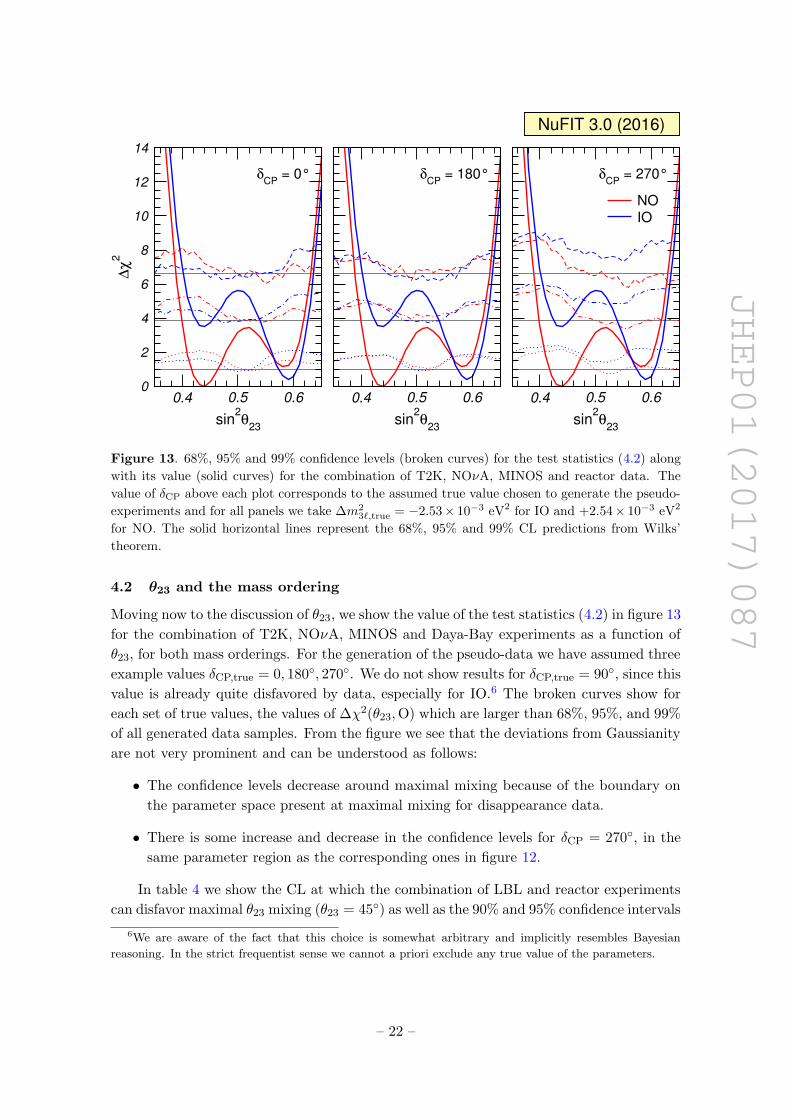
JHEP01(2017)087
0.4 0.5 0.6
sin2θ
23
0
2
4
6
8
10
12
14
∆χ
2
δCP
= 0°
0.4 0.5 0.6
sin2θ
23
δCP
= 180°
0.4 0.5 0.6
sin2θ
23
δCP
= 270°
NOIO
NuFIT 3.0 (2016)
Figure 13. 68%, 95% and 99% confidence levels (broken curves) for the test statistics (4.2) along
with its value (solid curves) for the combination of T2K, NOνA, MINOS and reactor data. The
value of δCP above each plot corresponds to the assumed true value chosen to generate the pseudo-
experiments and for all panels we take ∆m23`,true = −2.53× 10⁻³ eV2 for IO and +2.54× 10⁻³ eV2
for NO. The solid horizontal lines represent the 68%, 95% and 99% CL predictions from Wilks’
theorem.
4.2 θ23 and the mass ordering
Moving now to the discussion of θ23, we show the value of the test statistics (4.2) in figure 13
for the combination of T2K, NOνA, MINOS and Daya-Bay experiments as a function of
θ23, for both mass orderings. For the generation of the pseudo-data we have assumed three
example values δCP,true = 0, 180◦, 270◦. We do not show results for δCP,true = 90◦, since this
value is already quite disfavored by data, especially for IO.6 The broken curves show for
each set of true values, the values of ∆χ2(θ23,O) which are larger than 68%, 95%, and 99%
of all generated data samples. From the figure we see that the deviations from Gaussianity
are not very prominent and can be understood as follows:
• The confidence levels decrease around maximal mixing because of the boundary on
the parameter space present at maximal mixing for disappearance data.
• There is some increase and decrease in the confidence levels for δCP = 270◦, in the
same parameter region as the corresponding ones in figure 12.
In table 4 we show the CL at which the combination of LBL and reactor experiments
can disfavor maximal θ23 mixing (θ23 = 45◦) as well as the 90% and 95% confidence intervals
6We are aware of the fact that this choice is somewhat arbitrary and implicitly resembles Bayesian
reasoning. In the strict frequentist sense we cannot a priori exclude any true value of the parameters.
– 22 –
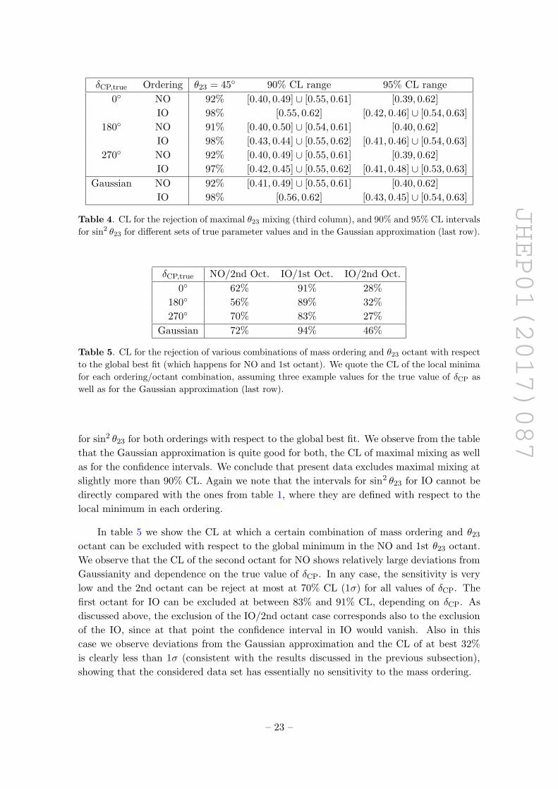
JHEP01(2017)087
δCP,true Ordering θ23 = 45◦ 90% CL range 95% CL range
0◦ NO 92% [0.40, 0.49] ∪ [0.55, 0.61] [0.39, 0.62]
IO 98% [0.55, 0.62] [0.42, 0.46] ∪ [0.54, 0.63]
180◦ NO 91% [0.40, 0.50] ∪ [0.54, 0.61] [0.40, 0.62]
IO 98% [0.43, 0.44] ∪ [0.55, 0.62] [0.41, 0.46] ∪ [0.54, 0.63]
270◦ NO 92% [0.40, 0.49] ∪ [0.55, 0.61] [0.39, 0.62]
IO 97% [0.42, 0.45] ∪ [0.55, 0.62] [0.41, 0.48] ∪ [0.53, 0.63]
Gaussian NO 92% [0.41, 0.49] ∪ [0.55, 0.61] [0.40, 0.62]
IO 98% [0.56, 0.62] [0.43, 0.45] ∪ [0.54, 0.63]
Table 4. CL for the rejection of maximal θ23 mixing (third column), and 90% and 95% CL intervals
for sin2 θ23 for different sets of true parameter values and in the Gaussian approximation (last row).
δCP,true NO/2nd Oct. IO/1st Oct. IO/2nd Oct.
0◦ 62% 91% 28%
180◦ 56% 89% 32%
270◦ 70% 83% 27%
Gaussian 72% 94% 46%
Table 5. CL for the rejection of various combinations of mass ordering and θ23 octant with respect
to the global best fit (which happens for NO and 1st octant). We quote the CL of the local minima
for each ordering/octant combination, assuming three example values for the true value of δCP as
well as for the Gaussian approximation (last row).
for sin2 θ23 for both orderings with respect to the global best fit. We observe from the table
that the Gaussian approximation is quite good for both, the CL of maximal mixing as well
as for the confidence intervals. We conclude that present data excludes maximal mixing at
slightly more than 90% CL. Again we note that the intervals for sin2 θ23 for IO cannot be
directly compared with the ones from table 1, where they are defined with respect to the
local minimum in each ordering.
In table 5 we show the CL at which a certain combination of mass ordering and θ23
octant can be excluded with respect to the global minimum in the NO and 1st θ23 octant.
We observe that the CL of the second octant for NO shows relatively large deviations from
Gaussianity and dependence on the true value of δCP. In any case, the sensitivity is very
low and the 2nd octant can be reject at most at 70% CL (1σ) for all values of δCP. The
first octant for IO can be excluded at between 83% and 91% CL, depending on δCP. As
discussed above, the exclusion of the IO/2nd octant case corresponds also to the exclusion
of the IO, since at that point the confidence interval in IO would vanish. Also in this
case we observe deviations from the Gaussian approximation and the CL of at best 32%
is clearly less than 1σ (consistent with the results discussed in the previous subsection),
showing that the considered data set has essentially no sensitivity to the mass ordering.
– 23 –
JHEP01(2017)087
5 Conclusions
We have presented the results of the updated (as of fall 2016) analysis of relevant neutrino
data in the framework of mixing among three massive neutrinos. Quantitatively the present
determination of the two mass differences, three mixing angles and the relevant CP violating
phase obtained under the assumption that their log-likelihood follows a χ2 distribution is
listed in table 1, and the corresponding leptonic mixing matrix is given in eq. (2.1). We
have found that the maximum allowed CP violation in the leptonic sector parametrized by
the Jarlskog determinant is JmaxCP = 0.0329± 0.0007 (+0.0021
−0.0024)) at 1σ (3σ).
We have studied in detail how the sensitivity to the least-determined parameters θ23,
δCP and the mass ordering depends on the proper combination of the different data samples
(section 3.2). Furthermore we have quantified deviations from the Gaussian approximation
in the evaluation of the confidence intervals for θ23 and δCP by performing a Monte Carlo
study of the long baseline accelerator and reactor results (section 4). We can summarize
the main conclusions in these sections as follows:
• At present the precision on the determination of |∆m23`| from νµ disappearance in
LBL accelerator experiments NOνA, T2K and MINOS is comparable to that from
νe disappearance in reactor experiments, in particular with the spectral information
from Daya-Bay. When comparing the region for each LBL experiment with that of
the reactor experiments we find some dispersion in the best fit values and allowed
ranges.
• The interpretation of the data from accelerator LBL experiments in the framework
of 3ν mixing requires using information from the reactor experiments, in particu-
lar about the mixing angle θ13. But since, as mentioned above, reactor data also
constrain |∆m23`|, the resulting CL of presently low confidence effects (in particular
the non-maximality of θ23 and the mass ordering) is affected by the inclusion of this
information in the combination.
• We find that the mass ordering favored by NOνA changes from NO to IO when the
information on ∆m23` from reactor experiments is correctly included in the LBL+REA
combination, and the ∆χ2 of NO in T2K is reduced from around 2 to 0.5 (see figure 7).
Our MC study of the combination of LBL and reactor data shows that for all cases
generated, NO is favored but with a CL of less than 1σ.
• About the non-maximality of θ23, we find that when the information on ∆m23` from
reactor experiments is correctly included in the LBL+REA combination, it is not
NOνA but actually MINOS which contributes most to the preference for non-maximal
θ23 (see figure 8). Quantitatively our MC study of the combination of LBL and reactor
data shows that for all the cases generated the CL for rejection of maximal θ23 is
about 92% for NO. As seen in figure 13 and table 4, the CL of maximal mixing as well
as confidence intervals for sin2 θ23 derived with MC simulations are not very different
from the corresponding Gaussian approximation.
– 24 –

JHEP01(2017)087
• The same study shows that for NO (IO) the favored octant is θ23 < 45◦ (θ23 > 45◦).
The CL for rejection of the disfavored octant depends on the true value of δCP
assumed in the MC study and it is generically lower than the one obtained in the
Gaussian limit (see table 5). For example, for NO the second octant is disfavored at a
confidence level between 0.9σ and 1.3σ depending on the assumed true value of δCP.
• The present sensitivity to δCP is driven by T2K with a minor contribution from NOνA
for IO (see figure 9). The dependence of the combined CL of the “hint” towards
leptonic CP violation and in particular for δCP ' 270◦ on the true value of θ23 is
shown in figure 12, from which we read that for all cases generated CP conservation
is disfavored only at 70% (1.05σ) for NO. Values of δCP ' 90◦ are disfavored at
around 99% CL for NO, while for IO the rejection is at higher CL (∆χ2 ' 14 with
respect to the global minimum).
Finally we comment that the increased statistics in SK4 and Borexino has had no major
impact in the long-standing tension between the best fit values of ∆m221 as determined
from the analysis of KamLAND and solar data, which remains an unresolved ∼ 2σ effect.
Future updates of this analysis will be provided at the NuFIT website quoted in
ref. [49].
Acknowledgments
This work is supported by USA-NSF grant PHY-1620628, by EU Networks FP10 ITN ELU-
SIVES (H2020-MSCA-ITN-2015-674896) and INVISIBLES-PLUS (H2020-MSCA-RISE-
2015-690575), by MINECO grants FPA2013-46570, FPA2012-31880 and MINECO/FEDER-
UE grant FPA2015-65929-P, by Maria de Maetzu program grant MDM-2014-0367 of IC-
CUB, and the “Severo Ochoa” program grant SEV-2012-0249 of IFT. I.E. acknowledges
support from the FPU program fellowship FPU15/03697.
A List of data used in the analysis
Solar experiments.
• Chlorine total rate [15], 1 data point.
• Gallex & GNO total rates [16], 2 data points.
• SAGE total rate [17], 1 data point.
• SK1 full energy and zenith spectrum [18], 44 data points.
• SK2 full energy and day/night spectrum [19], 33 data points.
• SK3 full energy and day/night spectrum [20], 42 data points.
• SK4 2055-day day-night asymmetry [21] and 2365-day energy spectrum [22], 24 data
points.
• SNO combined analysis [23], 7 data points.
– 25 –
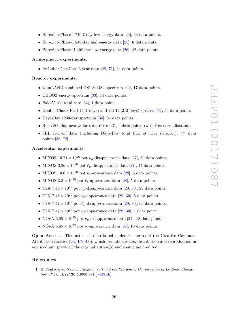
JHEP01(2017)087
• Borexino Phase-I 740.7-day low-energy data [24], 33 data points.
• Borexino Phase-I 246-day high-energy data [25], 6 data points.
• Borexino Phase-II 408-day low-energy data [26], 42 data points.
Atmospheric experiments.
• IceCube/DeepCore 3-year data [48, 71], 64 data points.
Reactor experiments.
• KamLAND combined DS1 & DS2 spectrum [32], 17 data points.
• CHOOZ energy spectrum [33], 14 data points.
• Palo-Verde total rate [34], 1 data point.
• Double-Chooz FD-I (461 days) and FD-II (212 days) spectra [35], 54 data points.
• Daya-Bay 1230-day spectrum [36], 34 data points.
• Reno 800-day near & far total rates [37], 2 data points (with free normalization).
• SBL reactor data (including Daya-Bay total flux at near detector), 77 data
points [38, 72].
Accelerator experiments.
• MINOS 10.71× 10²⁰ pot νµ-disappearance data [27], 39 data points.
• MINOS 3.36× 10²⁰ pot νµ-disappearance data [27], 14 data points.
• MINOS 10.6× 10²⁰ pot νe-appearance data [28], 5 data points.
• MINOS 3.3× 10²⁰ pot νe-appearance data [28], 5 data points.
• T2K 7.48× 10²⁰ pot νµ-disappearance data [29, 30], 28 data points.
• T2K 7.48× 10²⁰ pot νe-appearance data [29, 30], 5 data points.
• T2K 7.47× 10²⁰ pot νµ-disappearance data [29, 30], 63 data points.
• T2K 7.47× 10²⁰ pot νe-appearance data [29, 30], 1 data point.
• NOνA 6.05× 10²⁰ pot νµ-disappearance data [31], 18 data points.
• NOνA 6.05× 10²⁰ pot νe-appearance data [31], 10 data points.
Open Access. This article is distributed under the terms of the Creative Commons
Attribution License (CC-BY 4.0), which permits any use, distribution and reproduction in
any medium, provided the original author(s) and source are credited.
References
[1] B. Pontecorvo, Neutrino Experiments and the Problem of Conservation of Leptonic Charge,
Sov. Phys. JETP 26 (1968) 984 [INSPIRE].
– 26 –
JHEP01(2017)087
[2] V.N. Gribov and B. Pontecorvo, Neutrino astronomy and lepton charge, Phys. Lett. 28B
(1969) 493 [INSPIRE].
[3] M.C. Gonzalez-Garcia and M. Maltoni, Phenomenology with Massive Neutrinos, Phys. Rept.
460 (2008) 1 [arXiv:0704.1800] [INSPIRE].
[4] C. Giunti, Light Sterile Neutrinos: Status and Perspectives, Nucl. Phys. B 908 (2016) 336
[arXiv:1512.04758] [INSPIRE].
[5] Z. Maki, M. Nakagawa and S. Sakata, Remarks on the unified model of elementary particles,
Prog. Theor. Phys. 28 (1962) 870 [INSPIRE].
[6] M. Kobayashi and T. Maskawa, CP Violation in the Renormalizable Theory of Weak
Interaction, Prog. Theor. Phys. 49 (1973) 652 [INSPIRE].
[7] S.M. Bilenky, J. Hosek and S.T. Petcov, On Oscillations of Neutrinos with Dirac and
Majorana Masses, Phys. Lett. B 94 (1980) 495 [INSPIRE].
[8] P. Langacker, S.T. Petcov, G. Steigman and S. Toshev, On the Mikheev-Smirnov-Wolfenstein
(MSW) Mechanism of Amplification of Neutrino Oscillations in Matter, Nucl. Phys. B 282
(1987) 589 [INSPIRE].
[9] M.C. Gonzalez-Garcia, M. Maltoni and T. Schwetz, Updated fit to three neutrino mixing:
status of leptonic CP-violation, JHEP 11 (2014) 052 [arXiv:1409.5439] [INSPIRE].
[10] F. Capozzi, E. Lisi, A. Marrone, D. Montanino and A. Palazzo, Neutrino masses and
mixings: Status of known and unknown 3ν parameters, Nucl. Phys. B 908 (2016) 218
[arXiv:1601.07777] [INSPIRE].
[11] D.V. Forero, M. Tortola and J.W.F. Valle, Neutrino oscillations refitted, Phys. Rev. D 90
(2014) 093006 [arXiv:1405.7540] [INSPIRE].
[12] H. Minakata, H. Sugiyama, O. Yasuda, K. Inoue and F. Suekane, Reactor measurement of
theta(13) and its complementarity to long baseline experiments, Phys. Rev. D 68 (2003)
033017 [Erratum ibid. D 70 (2004) 059901] [hep-ph/0211111] [INSPIRE].
[13] P. Huber, M. Lindner, T. Schwetz and W. Winter, Reactor neutrino experiments compared to
superbeams, Nucl. Phys. B 665 (2003) 487 [hep-ph/0303232] [INSPIRE].
[14] P. Huber, M. Lindner, M. Rolinec, T. Schwetz and W. Winter, Prospects of accelerator and
reactor neutrino oscillation experiments for the coming ten years, Phys. Rev. D 70 (2004)
073014 [hep-ph/0403068] [INSPIRE].
[15] B.T. Cleveland et al., Measurement of the solar electron neutrino flux with the Homestake
chlorine detector, Astrophys. J. 496 (1998) 505 [INSPIRE].
[16] F. Kaether, W. Hampel, G. Heusser, J. Kiko and T. Kirsten, Reanalysis of the GALLEX
solar neutrino flux and source experiments, Phys. Lett. B 685 (2010) 47 [arXiv:1001.2731]
[INSPIRE].
[17] SAGE collaboration, J.N. Abdurashitov et al., Measurement of the solar neutrino capture
rate with gallium metal. III: Results for the 2002–2007 data-taking period, Phys. Rev. C 80
(2009) 015807 [arXiv:0901.2200] [INSPIRE].
[18] Super-Kamiokande collaboration, J. Hosaka et al., Solar neutrino measurements in
Super-Kamiokande-I, Phys. Rev. D 73 (2006) 112001 [hep-ex/0508053] [INSPIRE].
[19] Super-Kamiokande collaboration, J.P. Cravens et al., Solar neutrino measurements in
Super-Kamiokande-II, Phys. Rev. D 78 (2008) 032002 [arXiv:0803.4312] [INSPIRE].
– 27 –
JHEP01(2017)087
[20] Super-Kamiokande collaboration, K. Abe et al., Solar neutrino results in
Super-Kamiokande-III, Phys. Rev. D 83 (2011) 052010 [arXiv:1010.0118] [INSPIRE].
[21] Y. Nakano, 8B solar neutrino spectrum measurement using Super-Kamiokande IV, Ph.D.
thesis, Tokyo University, Tokyo, Japan (2016).
[22] Y. Nakano, Solar neutrino results from Super-Kamiokande, talk given at the 38th
International Conference on High Energy Physics, Chicago, U.S.A., 3–10 August 2016.
[23] SNO collaboration, B. Aharmim et al., Combined Analysis of all Three Phases of Solar
Neutrino Data from the Sudbury Neutrino Observatory, Phys. Rev. C 88 (2013) 025501
[arXiv:1109.0763] [INSPIRE].
[24] Borexino collaboration, G. Bellini et al., Precision measurement of the 7Be solar neutrino
interaction rate in Borexino, Phys. Rev. Lett. 107 (2011) 141302 [arXiv:1104.1816]
[INSPIRE].
[25] Borexino collaboration, G. Bellini et al., Measurement of the solar 8B neutrino rate with a
liquid scintillator target and 3 MeV energy threshold in the Borexino detector, Phys. Rev. D
82 (2010) 033006 [arXiv:0808.2868] [INSPIRE].
[26] Borexino collaboration, G. Bellini et al., Neutrinos from the primary proton-proton fusion
process in the Sun, Nature 512 (2014) 383 [INSPIRE].
[27] MINOS collaboration, P. Adamson et al., Measurement of Neutrino and Antineutrino
Oscillations Using Beam and Atmospheric Data in MINOS, Phys. Rev. Lett. 110 (2013)
251801 [arXiv:1304.6335] [INSPIRE].
[28] MINOS collaboration, P. Adamson et al., Electron neutrino and antineutrino appearance in
the full MINOS data sample, Phys. Rev. Lett. 110 (2013) 171801 [arXiv:1301.4581]
[INSPIRE].
[29] K. Iwamoto, Recent Results from T2K and Future Prospects, talk given at the 38th
International Conference on High Energy Physics, Chicago, U.S.A., 3–10 August 2016.
[30] A. Cervera, Latest Results from Neutrino Oscillation Experiments, talk given at the
SUSY 2016 Conference, Melbourne, Australia, 3–8 July 2016.
[31] P. Vahle, New results from NOvA, talk given at the XXVII International Conference on
Neutrino Physics and Astrophysics, London, U.K., 4–9 July 2016.
[32] KamLAND collaboration, A. Gando et al., Constraints on θ13 from A Three-Flavor
Oscillation Analysis of Reactor Antineutrinos at KamLAND, Phys. Rev. D 83 (2011) 052002
[arXiv:1009.4771] [INSPIRE].
[33] CHOOZ collaboration, M. Apollonio et al., Limits on neutrino oscillations from the
CHOOZ experiment, Phys. Lett. B 466 (1999) 415 [hep-ex/9907037] [INSPIRE].
[34] Palo Verde collaboration, A. Piepke, Final results from the Palo Verde neutrino oscillation
experiment, Prog. Part. Nucl. Phys. 48 (2002) 113 [INSPIRE].
[35] M. Ishitsuka, New results of Double Chooz, talk given at the Rencontres de Moriond EW
2016, La Thuile, Italy, 12–19 March 2016.
[36] Z. Yu, Recent Results from the Daya Bay Experiment, talk given at the XXVII International
Conference on Neutrino Physics and Astrophysics, London, U.K., 4–9 July 2016.
[37] S.-H. Seo, New Results from RENO, talk given at the XXVI International Conference on
Neutrino Physics and Astrophysics, Boston, U.S.A., 2–7 June 2014.
– 28 –

JHEP01(2017)087
[38] J. Kopp, P.A.N. Machado, M. Maltoni and T. Schwetz, Sterile Neutrino Oscillations: The
Global Picture, JHEP 05 (2013) 050 [arXiv:1303.3011] [INSPIRE].
[39] H. Kwon, F. Boehm, A.A. Hahn, H.E. Henrikson, J.L. Vuilleumier, J.F. Cavaignac et al.,
Search for Neutrino Oscillations at a Fission Reactor, Phys. Rev. D 24 (1981) 1097
[INSPIRE].
[40] CALTECH-SIN-TUM collaboration, G. Zacek et al., Neutrino Oscillation Experiments at
the Gosgen Nuclear Power Reactor, Phys. Rev. D 34 (1986) 2621 [INSPIRE].
[41] G.S. Vidyakin, V.N. Vyrodov, I.I. Gurevich, Yu. V. Kozlov, V.P. Martemyanov, S.V.
Sukhotin et al., Detection of Anti-neutrinos in the Flux From Two Reactors, Sov. Phys.
JETP 66 (1987) 243 [INSPIRE].
[42] G.S. Vidyakin et al., Limitations on the characteristics of neutrino oscillations, JETP Lett.
59 (1994) 390 [INSPIRE].
[43] A.I. Afonin, S.N. Ketov, V.I. Kopeikin, L.A. Mikaelyan, M.D. Skorokhvatov and S.V.
Tolokonnikov, A Study of the Reaction νe + P → e+ +N on a Nuclear Reactor, Sov. Phys.
JETP 67 (1988) 213 [INSPIRE].
[44] A.A. Kuvshinnikov, L.A. Mikaelyan, S.V. Nikolaev, M.D. Skorokhvatov and A.V. Etenko,
Measuring the νe + p→ n+ e+ cross-section and beta decay axial constant in a new
experiment at Rovno NPP reactor. (In Russian), JETP Lett. 54 (1991) 253 [INSPIRE].
[45] Y. Declais et al., Search for neutrino oscillations at 15-meters, 40-meters and 95-meters
from a nuclear power reactor at Bugey, Nucl. Phys. B 434 (1995) 503 [INSPIRE].
[46] Y. Declais et al., Study of reactor anti-neutrino interaction with proton at Bugey nuclear
power plant, Phys. Lett. B 338 (1994) 383 [INSPIRE].
[47] Z.D. Greenwood et al., Results of a two position reactor neutrino oscillation experiment,
Phys. Rev. D 53 (1996) 6054 [INSPIRE].
[48] IceCube collaboration, M.G. Aartsen et al., Determining neutrino oscillation parameters
from atmospheric muon neutrino disappearance with three years of IceCube DeepCore data,
Phys. Rev. D 91 (2015) 072004 [arXiv:1410.7227] [INSPIRE].
[49] NuFIT webpage, http://www.nu-fit.org.
[50] M.C. Gonzalez-Garcia, M. Maltoni, J. Salvado and T. Schwetz, Global fit to three neutrino
mixing: critical look at present precision, JHEP 12 (2012) 123 [arXiv:1209.3023] [INSPIRE].
[51] T.A. Mueller et al., Improved Predictions of Reactor Antineutrino Spectra, Phys. Rev. C 83
(2011) 054615 [arXiv:1101.2663] [INSPIRE].
[52] P. Huber, On the determination of anti-neutrino spectra from nuclear reactors, Phys. Rev. C
84 (2011) 024617 [Erratum ibid. C 85 (2012) 029901] [arXiv:1106.0687] [INSPIRE].
[53] G. Mention et al., The Reactor Antineutrino Anomaly, Phys. Rev. D 83 (2011) 073006
[arXiv:1101.2755] [INSPIRE].
[54] T. Schwetz, What is the probability that theta(13) and CP-violation will be discovered in
future neutrino oscillation experiments?, Phys. Lett. B 648 (2007) 54 [hep-ph/0612223]
[INSPIRE].
[55] M. Blennow, P. Coloma and E. Fernandez-Martinez, Reassessing the sensitivity to leptonic
CP-violation, JHEP 03 (2015) 005 [arXiv:1407.3274] [INSPIRE].
– 29 –
JHEP01(2017)087
[56] M.C. Gonzalez-Garcia and C. Pena-Garay, Three neutrino mixing after the first results from
K2K and KamLAND, Phys. Rev. D 68 (2003) 093003 [hep-ph/0306001] [INSPIRE].
[57] C. Jarlskog, Commutator of the Quark Mass Matrices in the Standard Electroweak Model
and a Measure of Maximal CP-violation, Phys. Rev. Lett. 55 (1985) 1039 [INSPIRE].
[58] Particle Data Group collaboration, C. Patrignani et al., Review of Particle Physics,
Chin. Phys. C 40 (2016) 100001 [INSPIRE].
[59] L. Wolfenstein, Neutrino Oscillations in Matter, Phys. Rev. D 17 (1978) 2369 [INSPIRE].
[60] S.P. Mikheev and A. Yu. Smirnov, Resonance Amplification of Oscillations in Matter and
Spectroscopy of Solar Neutrinos, Sov. J. Nucl. Phys. 42 (1985) 913 [INSPIRE].
[61] J. Bergstrom, M.C. Gonzalez-Garcia, M. Maltoni, C. Pena-Garay, A.M. Serenelli and
N. Song, Updated determination of the solar neutrino fluxes from solar neutrino data, JHEP
03 (2016) 132 [arXiv:1601.00972] [INSPIRE].
[62] N. Vinyoles et al., A new Generation of Standard Solar Models, arXiv:1611.09867
[INSPIRE].
[63] T.J.C. Bezerra, H. Furuta and F. Suekane, Measurement of Effective ∆m231 using Baseline
Differences of Daya Bay, RENO and Double CHOOZ Reactor Neutrino Experiments,
arXiv:1206.6017 [INSPIRE].
[64] H. Seo et al., Spectral Measurement of the Electron Antineutrino Oscillation Amplitude and
Frequency using 500 Live Days of RENO Data, arXiv:1610.04326 [INSPIRE].
[65] Super-Kamiokande collaboration, R. Wendell, Atmospheric Results from
Super-Kamiokande, AIP Conf. Proc. 1666 (2015) 100001 [arXiv:1412.5234] [INSPIRE].
[66] J. Kameda, Recent results from Super-Kamokande on atmospheric neutrinos and next
project: Hyper-Kamioande, talk given at the XII Rencontres de Vietnam: NuFact 2016, Qui
Nhon, Vietnam, 21–27 August 2016.
[67] K. P. Lee, Study of the neutrino mass hierarchy with the atmospheric neutrino data observed
in SuperKamiokande, Ph.D. thesis, The University of Tokyo, Tokyo, Japan (2012).
[68] J. Elevant and T. Schwetz, On the determination of the leptonic CP phase, JHEP 09 (2015)
016 [arXiv:1506.07685] [INSPIRE].
[69] M. Blennow, P. Coloma, P. Huber and T. Schwetz, Quantifying the sensitivity of oscillation
experiments to the neutrino mass ordering, JHEP 03 (2014) 028 [arXiv:1311.1822]
[INSPIRE].
[70] S.S. Wilks, The Large-Sample Distribution of the Likelihood Ratio for Testing Composite
Hypotheses, Annals Math. Statist. 9 (1938) 60.
[71] IceCube collaboration, J.P. Yanez et al., IceCube Oscillations: 3 years muon neutrino
disappearance data, http://icecube.wisc.edu/science/data/nu osc.
[72] C. Zhang, Recent Results From Daya Bay, talk given at the XXVI International Conference
on Neutrino Physics and Astrophysics, Boston, U.S.A., 2–7 June 2014.
– 30 –
Chapter3
Double-Cascades Events from NewPhysics in IceCube
SM can be considered as low energy effective model, so it can be extended byintroducing higher-dimension operators in terms of the SM fields
Leff = LSM +Ld=5
Λ+
Ld=6
Λ2+ · · · (3.1)
where Λ is the cutoff scale of the effective field theory. The lowest dimensionaloperator that generates Majorana neutrino masses after the Higgs mechanism is thedimensional five operator, called Weinberg operator. Which is the only possibled = 5 operator [33]
Ld=5
Λ=
1
2cd=5αβ
(LcLαΦ∗
)(Φ†LLβ
)(3.2)
where LL is the lepton doublet (Table 1.1), Φ = ıσ2Φ∗, σ2 is the Pauli matrix andΦ = (φ+, φ0)T is the standard Higgs doublet. cd=5
αβ ∼ 1/Λ is a model independentcoefficient of inverse mass dimension, which is suppressed by the scale Λ. Afterthe electroweak symmetry breaking, the neutrino gets a mass of the order mν ∼〈Φ〉2 /Λ. For o(1) couplings, the scale is of the order of the Grand Unified TheoryΛ ≥ 1013 GeV.
There are only three ways to generate the Weinberg operator at tree level, theyare called the see-saw models [34, 35], (Sec. 1.3.1). In the Type-I see-saw, themediator is a singlet fermion. In the Type-II see-saw, a triplet scalar is added intothe SM. In the Type-III see-saw, a triplet fermion works as a mediator. For eachof the three see-saw models, we can obtain a d = 5 operator by integrating out theheavy degrees of freedom.
In the next work, we have considered the Type-I see-saw with a mediator atthe scale of 1 GeV. In order to generate neutrino masses (< eV) [16] it is neededan additional suppression mechanism for the neutrino masses. The most studiedare [34]:
- The generation of the neutrino mass by loop corrections [36].
- The additional suppression of the neutrino mass due to a small lepton numberviolation [37, 38].
- The generation of the neutrino masses by higher dimensional operators [39],where the d = 5 operators is suppressed.
71

Double-Cascade Events from New Physics in Icecube
Pilar Coloma,1,* Pedro A. N. Machado,1,† Ivan Martinez-Soler,2,‡ and Ian M. Shoemaker3,§1Theory Department, Fermi National Accelerator Laboratory, Post Office Box 500, Batavia, Illinois 60510, USA
2Instituto de Fisica Teorica UAM-CSIC, Calle Nicolas Cabrera 13-15, Universidad Autonoma de Madrid,Cantoblanco, E-28049 Madrid, Spain
3Department of Physics, University of South Dakota, Vermillion, South Dakota 57069, USA(Received 18 August 2017; published 16 November 2017)
A variety of new physics models allows for neutrinos to up-scatter into heavier states. If the incidentneutrino is energetic enough, the heavy neutrino may travel some distance before decaying. In this work,we consider the atmospheric neutrino flux as a source of such events. At IceCube, this would lead to a“double-bang” (DB) event topology, similar to what is predicted to occur for tau neutrinos at ultrahighenergies. The DB event topology has an extremely low background rate from coincident atmosphericcascades, making this a distinctive signature of new physics. Our results indicate that IceCube should alreadybe able to derive new competitive constraints onmodels with GeV-scale sterile neutrinos using existing data.
DOI: 10.1103/PhysRevLett.119.201804
Introduction.—Although neutrino physics has rapidlymoved into the precision era, a number of fundamentalquestions remain unanswered. Perhaps the most importantamong these is the mechanism responsible for neutrinomasses. In the most naïve extension of the standard model(SM), neutrino masses and mixing can be successfullygenerated by adding at least two right-handed neutrinos(NR), with small Yukawa couplings Yν to the left-handedlepton doublets LL and the Higgs boson ϕ. In thisframework, Dirac neutrino masses are generated afterelectroweak (EW) symmetry breaking, as for the rest ofthe SM fermions. As singlets of the SM the right-handedneutrinos may also have a Majorana mass term, since it isallowed by gauge symmetry. In this case, the neutrino massLagrangian reads
Lνmass ⊃ YνLLϕNR þ 1
2MRNc
RNR þ H:c:;
where ϕ≡ iσ2ϕ�,NcR ≡ CNT
R is the charge conjugate ofNRand we have omitted flavor and mass indices. This is thewell-known type I seesaw Lagrangian [1–3]. Traditionally,the type I seesaw assumed a very high Majorana mass scaleMR. ForMR ≫ v the light neutrino masses are proportionalto mν ∝ Y†
νM−1R Yνv2, where v is the Higgs vacuum expect-
ation value, while the right-handed neutrino masses wouldbe approximately mN ≃MR þOðmνÞ. In this frameworkthe SM neutrino masses are naturally suppressed by thenew physics scale and can be much smaller than thecharged fermion masses without the need for tinyYukawa couplings. However, such heavy neutrinos aretoo heavy to be produced in colliders, and the inclusion ofvery massive Majorana neutrinos would considerablyworsen the hierarchy problem for the Higgs mass [4].Models with lower values of mN can lead to a
more interesting phenomenology, testable at low-energy
experiments, and possibly even solve some of the otherproblems of the SM. For example, keV neutrinos offer avery good dark matter candidate [5], while Majorananeutrinos with masses mN ∼Oð1–100Þ GeV can success-fully generate the matter-antimatter asymmetry of theUniverse [6–9]. While right-handed neutrinos with massesabove the EW scale are subject to very tight bounds fromEWobservables and charged lepton flavor violating experi-ments [10,11], these constraints fade away for lowermasses. Indeed, for right-handed neutrinos in the (keV–GeV) range, the strongest constraints come from precisionmeasurements of meson decays [12,13], muon decays, andother EW transitions; see, e.g., Ref. [14] for a review.In this Letter we point out that IceCube and DeepCore
can be used to test models with GeV neutrinos directly. Tothis end, we consider events with a “double-bang” (DB)topology. A schematic illustration of the event topology canbe seen in Fig. 1. In the first interaction, an atmosphericneutrino would up-scatter off a nucleus into a heavier state.This generally leaves a visible shower (or cascade) in the
FIG. 1. Schematic illustration of a DB event in IceCube. Anincoming active neutrino ν up-scatters into a heavy neutrino N,which then propagates and decays into SM particles. The smallcircles represent the DOMs while the large circles indicate thepositions where energy was deposited.
PRL 119, 201804 (2017) P HY S I CA L R EV I EW LE T T ER Sweek ending
17 NOVEMBER 2017
0031-9007=17=119(20)=201804(5) 201804-1 © 2017 American Physical Society
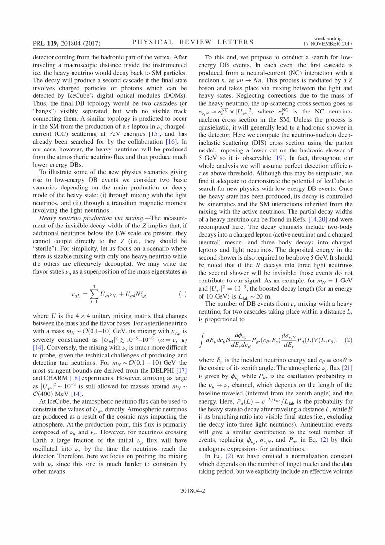
detector coming from the hadronic part of the vertex. Aftertraveling a macroscopic distance inside the instrumentedice, the heavy neutrino would decay back to SM particles.The decay will produce a second cascade if the final stateinvolves charged particles or photons which can bedetected by IceCube’s digital optical modules (DOMs).Thus, the final DB topology would be two cascades (or“bangs”) visibly separated, but with no visible trackconnecting them. A similar topology is predicted to occurin the SM from the production of a τ lepton in ντ charged-current (CC) scattering at PeV energies [15], and hasalready been searched for by the collaboration [16]. Inour case, however, the heavy neutrinos will be producedfrom the atmospheric neutrino flux and thus produce muchlower energy DBs.To illustrate some of the new physics scenarios giving
rise to low-energy DB events we consider two basicscenarios depending on the main production or decaymode of the heavy state: (i) through mixing with the lightneutrinos, and (ii) through a transition magnetic momentinvolving the light neutrinos.Heavy neutrino production via mixing.—The measure-
ment of the invisible decay width of the Z implies that, ifadditional neutrinos below the EW scale are present, theycannot couple directly to the Z (i.e., they should be“sterile”). For simplicity, let us focus on a scenario wherethere is sizable mixing with only one heavy neutrino whilethe others are effectively decoupled. We may write theflavor states να as a superposition of the mass eigenstates as
ναL ¼X3i¼1
UαiνiL þ Uα4Nc4R; ð1Þ
where U is the 4 × 4 unitary mixing matrix that changesbetween the mass and the flavor bases. For a sterile neutrinowith a mass mN ∼Oð0.1–10Þ GeV, its mixing with νe;μ isseverely constrained as jUα4j2 ≲ 10−5–10−8 (α ¼ e, μ)[14]. Conversely, the mixing with ντ is much more difficultto probe, given the technical challenges of producing anddetecting tau neutrinos. For mN ∼Oð0.1 − 10Þ GeV themost stringent bounds are derived from the DELPHI [17]and CHARM [18] experiments. However, a mixing as largeas jUτ4j2 ∼ 10−2 is still allowed for masses around mN ∼Oð400Þ MeV [14].At IceCube, the atmospheric neutrino flux can be used to
constrain the values of Uα4 directly. Atmospheric neutrinosare produced as a result of the cosmic rays impacting theatmosphere. At the production point, this flux is primarilycomposed of νμ and νe. However, for neutrinos crossingEarth a large fraction of the initial νμ flux will haveoscillated into ντ by the time the neutrinos reach thedetector. Therefore, here we focus on probing the mixingwith ντ since this one is much harder to constrain byother means.
To this end, we propose to conduct a search for low-energy DB events. In each event the first cascade isproduced from a neutral-current (NC) interaction with anucleon n, as νn → Nn. This process is mediated by a Zboson and takes place via mixing between the light andheavy states. Neglecting corrections due to the mass ofthe heavy neutrino, the up-scattering cross section goes asσντN ≃ σNCν × jUτ4j2, where σNCν is the NC neutrino-nucleon cross section in the SM. Unless the process isquasielastic, it will generally lead to a hadronic shower inthe detector. Here we compute the neutrino-nucleon deep-inelastic scattering (DIS) cross section using the partonmodel, imposing a lower cut on the hadronic shower of5 GeV so it is observable [19]. In fact, throughout ourwhole analysis we will assume perfect detection efficien-cies above threshold. Although this may be simplistic, wefind it adequate to demonstrate the potential of IceCube tosearch for new physics with low energy DB events. Oncethe heavy state has been produced, its decay is controlledby kinematics and the SM interactions inherited from themixing with the active neutrinos. The partial decay widthsof a heavy neutrino can be found in Refs. [14,20] and wererecomputed here. The decay channels include two-bodydecays into a charged lepton (active neutrino) and a charged(neutral) meson, and three body decays into chargedleptons and light neutrinos. The deposited energy in thesecond shower is also required to be above 5 GeV. It shouldbe noted that if the N decays into three light neutrinosthe second shower will be invisible: those events do notcontribute to our signal. As an example, for mN ¼ 1 GeVand jUτ4j2 ¼ 10−3, the boosted decay length (for an energyof 10 GeV) is Llab ∼ 20 m.The number of DB events from ντ mixing with a heavy
neutrino, for two cascades taking place within a distance L,is proportional to
ZdEνdcθB
dϕνμ
dEνdcθPμτðcθ;EνÞ
dσντNdEν
PdðLÞVðL;cθÞ; ð2Þ
where Eν is the incident neutrino energy and cθ ≡ cos θ isthe cosine of its zenith angle. The atmospheric νμ flux [21]is given by ϕνμ while Pμτ is the oscillation probability inthe νμ → ντ channel, which depends on the length of thebaseline traveled (inferred from the zenith angle) and theenergy. Here, PdðLÞ ¼ e−L=Llab=Llab is the probability forthe heavy state to decay after traveling a distance L, while Bis its branching ratio into visible final states (i.e., excludingthe decay into three light neutrinos). Antineutrino eventswill give a similar contribution to the total number ofevents, replacing ϕνμ , σντN , and Pμτ in Eq. (2) by theiranalogous expressions for antineutrinos.In Eq. (2) we have omitted a normalization constant
which depends on the number of target nuclei and the datataking period, but we explicitly include an effective volume
PRL 119, 201804 (2017) P HY S I CA L R EV I EW LE T T ER Sweek ending
17 NOVEMBER 2017
201804-2

VðL; cθÞ. In this work, this was computed usingMonte Carlo integration. First, for triggering purposeswe require that at least three (four) DOMs detect the firstshower simultaneously, if it takes place inside (outside)DeepCore [22]. Once the trigger goes off, all the informa-tion in the detector is recorded, and we thus assume that thesecond shower is always observed as long as it is closeenough to a DOM. Eventually, the energy of a cascadedetermines the distance from which it can be detected by aDOM: the longer the distance, the more energetic thecascade should be so the light can reach the DOM withoutbeing absorbed by the ice first. Here we assume that acascade is seen by a DOM if it takes place within a distanceof 36 m, since this is roughly the maximum distancebetween an event and a DOM inside DeepCore [22]. This isconservative, since showers with energies much above5 GeV will typically reach a DOM from longer distances.Finally, a minimum separation is required between the twoshowers so they can be resolved. This ultimately dependson the time resolution of the DOMs. Following Ref. [16],IceCube can distinguish pulses separated by T ∼ 66 ns.Thus, we require a minimum distance between the twoshowers of T=c ¼ 20 m.The dominant source of background for DB events is
given by two coincident cascades taking place within thesame time window Δt. The rate can be estimated as [23]Nbkg ≃ C2
DBðΔt=TÞ2, where C2DB ¼ NcascðNcasc − 1Þ=2
comes from the number of possible combination of pairs,and Ncasc is the number of cascade events within a timeperiod T. The number of cascades in the DeepCore volume,with a deposited energy between 5.6 and 100 GeV, isNcasc ≃ 2 × 10⁴ yr−1 [24]. These include CC events withelectrons, taus, or low-energy muons in the final state(which do not leave long identificable tracks), as well asNC events. A particle traveling at the speed of lighttraverses 1 km in ∼10−5 s. Thus, for a conservative timeinterval Δt ¼ 10−3 s, we get Nbkg < 10−11 yr−1.In view of the negligible background rate, we proceed to
determine the region in parameter space where at least onesignal event would be expected in six years of data takingat IceCube. This is shown in Fig. 2 as a function of themass and mixing of the heavy neutrino. The solid lineshows the results using the full IceCube volume, while forthe dashed line only DeepCore was considered. Our resultsindicate that IceCube could improve over present boundsbetween 1 and 2 orders of magnitude, and probe values ofthe mixing as small as jUτ4j2 ∼ 5 × 10⁻⁵. According tothese results, IceCube could test the proposed solutionto the flavor anomalies in the B sector proposed inRef. [25].Heavy neutrino production via a transition magnetic
moment.—Alternatively, the light neutrinos may interactwith the heavy state N through a higher-dimensionaloperator. As an example, we consider a neutrino transitionmagnetic moment (NTMM) μtr:
Lν ⊃ −μtrναLσρσN4RFρσ; ð3Þ
where Fρσ is the electromagnetic field strength tensor andσρσ ¼ ði=2Þ½γρ; γσ�. For simplicity, in this scenario weassume negligible mixing with the light neutrinos, so boththe production and decay of the heavy neutrino are con-trolled by the magnetic moment operator. In the rest frameof N, its decay width reads ΓðN → νγÞ ¼ μ2trM3=ð16πÞ.For mN ¼ 100 MeV, μtr ¼ 10−8μB (where μB is the Bohrmagneton), and a typical energy of 10 GeV this gives adecay length in the lab frame Llab ∼ 14 m.Neutrinos with a NTMM could scatter off both electrons
and nuclei in the IceCube detector. However, for the rangeof energies and masses considered in this work, the largesteffect comes from scattering on nuclei. In the DIS regime,the cross section for the scattering νn → Nn via theoperator in Eq. (3) reads [26]
d2σνn→Nn
dxdy≃ 16παμ2tr
�1 − yy
�Xi
e2i fiðxÞ; ð4Þ
where α is the fine structure constant, fiðxÞ is the partondistribution function for the parton i, x is the partonmomentum fraction, and e2i is its electric charge. Here,y≡ 1 − EN=Eν ¼ Er=Eν, where EN is the energy of theoutgoing heavy neutrino and Er is the deposited energy. InEq. (4) we have ignored the impact of the heavy neutrinomass in the cross section, which will be negligible in theregion of interest. However, energy and momentum con-servation requires
FIG. 2. Expected potential of IceCube to constrain the mixingbetween ντ and a heavy neutrino. In the region enclosed by thesolid green contour, more than one DB event is expected duringsix years of data taking at IceCube. The dashed contour shows themost conservative result, where only the DeepCore volume isconsidered. The shaded regions are disfavored by CHARM [18]and DELPHI [17] at 90% and 95% C.L., respectively; seeRef. [14].
PRL 119, 201804 (2017) P HY S I CA L R EV I EW LE T T ER Sweek ending
17 NOVEMBER 2017
201804-3
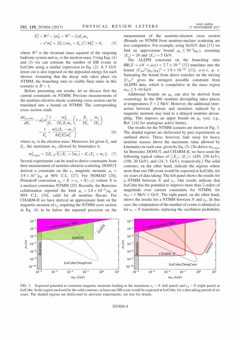
E2r −W2 − ½m2
N −W2 − 2xEνmn
− x2m2n þ 2Erðxmn þ EνÞ�2=4E2
ν > 0; ð5Þ
where W2 is the invariant mass squared of the outgoinghadronic system andmn is the nucleon mass. Using Eqs. (4)and (5) we can estimate the number of DB events inIceCube using a similar expression to Eq. (2). A 5 GeVlower cut is also imposed on the deposited energy for eachshower. Assuming that the decay only takes place viaNTMM, the branching ratio to visible final states in thisscenario is B ¼ 1.Before presenting our results, let us discuss first the
current constraints on NTMM. Previous measurements ofthe neutrino-electron elastic scattering cross section can betranslated into a bound on NTMM. The correspondingcross section reads
dσνe→Ne
dEr¼ μ2trα
�1
Er−
m2N
2EνErme
�1 −
Er
2Eνþ me
2Eν
�
−1
Eνþm4
NðEr −meÞ8E2
νE2rm2
e
�; ð6Þ
where me is the electron mass. Moreover, for given Eν andEr, the maximum mN allowed by kinematics is
m2N;max ¼ 2½Eν
ffiffiffiffiffiffiffiffiffiffiffiffiffiffiffiffiffiffiffiffiffiffiffiffiffiffiffiffiErðEr þ 2meÞ
p− ErðEν þmeÞ�: ð7Þ
Several experiments can be used to derive constraints fromtheir measurement of neutrino-electron scattering. DONUTderived a constraint on the ντ magnetic moment, μτ <3.9 × 10⁻⁷μB at 90% C.L. [27]. For NOMAD [28],Primakoff conversion νμ þ X → νs þ XðþγÞ (where X isa nucleus) constrains NTMM [29]. Recently, the Borexinocollaboration reported the limit μν < 2.8 × 10⁻¹¹μB at90% C.L. [30], valid for all neutrino flavors. ForCHARM-II we have derived an approximate limit on themagnetic moment of νμ requiring the NTMM cross sectionin Eq. (6) to be below the reported precision on the
measurement of the neutrino-electron cross section(Bounds on NTMM from neutrino-nucleus scattering areless competitive. For example, using NuTeV data [31] wefind an approximate bound μtr ≲ 10−4μB.), assuminghEνi ∼ 24 and hEri ∼ 5 GeV.The ALEPH constraint on the branching ratio
BRðZ → νN → ννγÞ < 2.7 × 10⁻⁵ [32] translates into thebound jUα4j2ðμtr=μBÞ2 < 1.9 × 10⁻¹⁶ [33], α≡ e, μ, τ.Saturating the bound from direct searches on the mixingjUτ4j2 gives the strongest possible constraint fromALEPH data, which is competitive in the mass regionmN ≳ 5–10 GeV.Additional bounds on μtr can also be derived from
cosmology. In the SM, neutrino decoupling takes placesat temperatures T ∼ 2 MeV. However, the additional inter-action between photons and neutrinos induced by amagnetic moment may lead to a delayed neutrino decou-pling. This imposes an upper bound on μtr (see, e.g.,Ref. [34] for analogous active limits).Our results for the NTMM scenario are shown in Fig. 3.
The shaded regions are disfavored by past experiments asoutlined above. These, however, fade away for heavyneutrino masses above the maximum value allowed bykinematics in each case, given by Eq. (5). [To derivemN;max
for Borexino, DONUT, and CHARM-II, we have used thefollowing typical values of ðhEνi; hEriÞ: (420, 230 keV),(100, 20 GeV), and (24, 5 GeV), respectively.] The solidcontours, on the other hand, indicate the regions wheremore than one DB event would be expected at IceCube, forsix years of data taking. The left panel shows the results fora NTMM between N and ντ. Our results indicate thatIceCube has the potential to improve more than 2 orders ofmagnitude over current constraints for NTMM, formN ∼ 1 MeV–1 GeV. The right panel, on the other hand,shows the results for a NTMM between N and νμ. In thiscase, the computation of the number of events is identical asfor ντ − N transitions, replacing the oscillation probability
FIG. 3. Expected potential to constrain magnetic moments leading to the transitions ντ − N (left panel) and νμ − N (right panel) atIceCube. In the region enclosed by the solid contours, at least one DB event would be expected at IceCube, for a data taking period of sixyears. The shaded regions are disfavored by previous experiments; see text for details.
PRL 119, 201804 (2017) P HY S I CA L R EV I EW LE T T ER Sweek ending
17 NOVEMBER 2017
201804-4
Pμτ by Pμμ in Eq. (2). Even though current constraints arestronger for νμ, we also find that IceCube could signifi-cantly improve over present bounds.Conclusions.—In this Letter, we have studied the poten-
tial of the IceCube detector to look for new physics usinglow-energy DB events. The collaboration has alreadyperformed searches for events with this topology at ultra-high energies, which are expected in the SM from the CCinteractions of PeV tau neutrinos. In this work we haveshown how very simple new physics scenarios with GeV-scale right-handed neutrinos would lead to a similar top-ology, with two low-energy cascades that could be spatiallyresolved in the detector. We find that IceCube may be ableto improve by orders of magnitude the current constraintson the two scenarios considered here. A DB search mayalso be sensitive to nonminimal dark matter models, such asthe one proposed in Ref. [35].
We warmly thank Tyce de Young for useful discussionson the IceCube detector performance. We are very gratefulas well for insightful discussions with Kaladi Babu,Enrique Fernandez-Martinez, Jacobo Lopez-Pavon,Kohta Murase, and Josef Pradler. This work receivedpartial support from the European Union through theElusives (H2020-MSCA-ITN-2015-674896) andInvisiblesPlus (H2020-MSCA-RISE-2015-690575) grants.I. M.-S. is very grateful to the University of South Dakotafor its support. I. M-S. acknowledges support through theSpanish Grants No. FPA2015-65929-P (MINECO/FEDER, UE) and the Spanish Research Agency(Agencia Estatal de Investigación) through the GrantsIFT “Centro de Excelencia Severo Ochoa” SEV-2012-0249 and SEV-2016-0597, and would like to thank theFermilab theory department for their kind hospitalityduring his visits, where this work was started. Thismanuscript has been authored by Fermi ResearchAlliance, LLC under Contract No. DE-AC02-07CH11359 with the U.S. Department of Energy, Officeof Science, Office of High Energy Physics. The publisher,by accepting the article for publication, acknowledges thatthe United States Government retains a non-exclusive,paid-up, irrevocable, world-wide license to publish orreproduce the published form of this manuscript, or allowothers to do so, for United States Government purposes.
*[email protected]†[email protected]‡[email protected]§[email protected]
[1] P. Minkowski, Phys. Lett. 67B, 421 (1977).[2] M. Gell-Mann, P. Ramond, and R. Slansky, Conference
Proceedings C790927, 315 (1979).[3] R. N. Mohapatra and G. Senjanovic, Phys. Rev. Lett. 44,
912 (1980).[4] F. Vissani, Phys. Rev. D 57, 7027 (1998).
[5] A. Kusenko, Phys. Rep. 481, 1 (2009).[6] T. Asaka, S. Blanchet, and M. Shaposhnikov, Phys. Lett. B
631, 151 (2005).[7] T. Asaka and M. Shaposhnikov, Phys. Lett. B 620, 17
(2005).[8] P. Hernández, M. Kekic, J. López-Pavón, J. Racker, and
J. Salvado, J. High Energy Phys. 08 (2016) 157.[9] P. Hernández, M. Kekic, J. López-Pavón, J. Racker, and
N. Rius, J. High Energy Phys. 10 (2015) 067.[10] S. Antusch and O. Fischer, J. High Energy Phys. 10 (2014)
094.[11] E. Fernandez-Martinez, J. Hernandez-Garcia, and J. Lopez-
Pavon, J. High Energy Phys. 08 (2016) 033.[12] R. E. Shrock, Phys. Lett. 96B, 159 (1980).[13] R. E. Shrock, Phys. Rev. D 24, 1232 (1981).[14] A. Atre, T. Han, S. Pascoli, and B. Zhang, J. High Energy
Phys. 05 (2009) 030.[15] J. G. Learned and S. Pakvasa, Astropart. Phys. 3, 267 (1995).[16] M. G. Aartsen et al. (IceCube Collaboration), Phys. Rev. D
93, 022001 (2016).[17] P. Abreu et al., Z. Phys. C 74, 57 (1997); 75, 580E (1997).[18] J. Orloff, A. N. Rozanov, and C. Santoni, Phys. Lett. B 550,
8 (2002).[19] M. G. Aartsen et al. (IceCube Collaboration), arXiv:
1707.07081.[20] D. Gorbunov and M. Shaposhnikov, J. High Energy Phys.
10 (2007) 015; 11 (2013) 101E.11 (2013) 101(E).[21] M. Honda, M. S. Athar, T. Kajita, K. Kasahara, and
S. Midorikawa, Phys. Rev. D 92, 023004 (2015).[22] M. G. Aartsen et al. (IceCube Collaboration), J. Instrum. 12,
P03012 (2017).[23] S.-F. Ge, M. Lindner, and W. Rodejohann, Phys. Lett. B
772, 164 (2017).[24] J. Hignight, Measurements of atmospheric NuMu disap-
pearance with IceCube-DeepCore (2017), talk given at theLake Louise Winter Institute 2017, https://indico.cern.ch/event/531113/contributions/2430431/.
[25] G. Cvetič, F. Halzen, C. S. Kim, and S. Oh, arXiv:1702.04335.
[26] See Supplemental Material at http://link.aps.org/supplemental/10.1103/PhysRevLett.119.201804 for detailson the computation of the cross section for the scatteringνn → Nn via a transition magnetic moment.
[27] R. Schwienhorst et al. (DONUT Collaboration), Phys. Lett.B 513, 23 (2001).
[28] J. Altegoer et al. (NOMAD Collaboration), Nucl. Instrum.Methods Phys. Res., Sect. A 404, 96 (1998).
[29] S. N. Gninenko and N. V. Krasnikov, Phys. Lett. B 450, 165(1999).
[30] M. Agostini et al. (Borexino Collaboration), arXiv:1707.09355.
[31] G. P. Zeller et al. (NuTeV Collaboration), Phys. Rev. Lett.88, 091802 (2002); 90, 239902E (2003).
[32] D. Decamp et al. (ALEPH Collaboration), Phys. Rep. 216,253 (1992).
[33] S. N. Gninenko, Phys. Rev. D 83, 015015 (2011).[34] N. Vassh, E. Grohs, A. B. Balantekin, and G. M. Fuller,
Phys. Rev. D 92, 125020 (2015).[35] D. Kim, J.-C. Park, and S. Shin, Phys. Rev. Lett. 119,
161801 (2017).
PRL 119, 201804 (2017) P HY S I CA L R EV I EW LE T T ER Sweek ending
17 NOVEMBER 2017
201804-5

Chapter4
Non-standard neutrino interactions in theEarth and the flavor of astrophysical
neutrinos
In the expansion of the SM lagrangian with higher dimensional operators (eq (3.1)),the operators with d = 5 correspond to a neutrino mass term, called Weinberg op-erator. For d = 6, there are some operators that lead the so-called Non-StandardInteractions (NSI) in the neutrino sector [40]
(ναγρPLνβ)
(fγρPf
)(4.1)
(ναγρPLlβ)
(f ′γρPf
)(4.2)
where f and f ′ correspond to charged fermion fields. PL = (1 − γ5)/2 is the left-handed projector, while P can be either PL or PR (right-handed projector). Theseoperators introduce a modification of the neutrino interaction with the chargedfermions, which affect to the neutrino production and detection by a new charged-current interaction Eq (4.2), and a new neutral-current interaction Eq (4.1). At zeromomentum transfer, the NSI-NC can modify the matter potential that describesthe neutrino evolution through the matter, and their effect can be enhanced whenneutrinos travel long distances through the matter. This is the case of atmosphericneutrinos experiments. As we are going to see in the following work, the new matterpotential can also have an observable effect on the flavor of astrophysical neutrinos.
The operators Eqs (4.2) (4.1) are not singlets of the SM symmetry group Eq (1.1).In order to promote them to a gauge invariant operator, for instance, we can replacethe fermion fields by the SU(2) doublets. In this case, the operators Eqs (4.2) (4.1)could be obtained from
(LαLγρLβL)(LγLγ
ρLδL) (4.3)
(LαLγρLβL)(QγLγ
ρQδL) (4.4)
In addition to the new interaction for neutrinos, the gauge invariant operators bringnew interactions between the charged fermions like µ → 3e that are tight con-strained [41, 10]. In the order to avoid these constraints it is needed cancellationsamong the different higher-dimensional operators [42, 43].
77
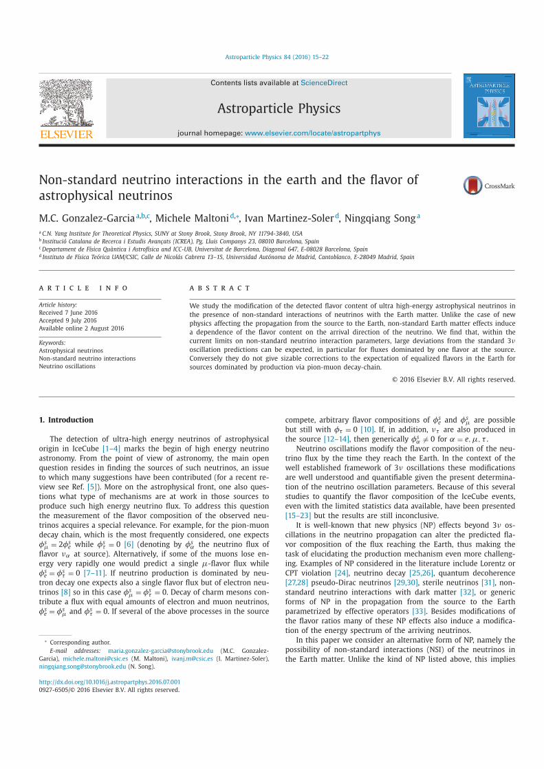
Astroparticle Physics 84 (2016) 15–22
Contents lists available at ScienceDirect
Astroparticle Physics
journal homepage: www.elsevier.com/locate/astropartphys
Non-standard neutrino interactions in the earth and the flavor of
astrophysical neutrinos
M.C. Gonzalez-Garcia
a , b , c , Michele Maltoni d , ∗, Ivan Martinez-Soler d , Ningqiang Song
a
a C.N. Yang Institute for Theoretical Physics, SUNY at Stony Brook, Stony Brook, NY 11794-3840, USA b Institució Catalana de Recerca i Estudis Avançats (ICREA), Pg. Lluis Companys 23, 08010 Barcelona, Spain c Departament de Física Quàntica i Astrofísica and ICC-UB, Universitat de Barcelona, Diagonal 647, E-08028 Barcelona, Spain d Instituto de Física Teórica UAM/CSIC, Calle de Nicolás Cabrera 13–15, Universidad Autónoma de Madrid, Cantoblanco, E-28049 Madrid, Spain
a r t i c l e i n f o
Article history:
Received 7 June 2016
Accepted 9 July 2016
Available online 2 August 2016
Keywords:
Astrophysical neutrinos
Non-standard neutrino interactions
Neutrino oscillations
a b s t r a c t
We study the modification of the detected flavor content of ultra high-energy astrophysical neutrinos in
the presence of non-standard interactions of neutrinos with the Earth matter. Unlike the case of new
physics affecting the propagation from the source to the Earth, non-standard Earth matter effects induce
a dependence of the flavor content on the arrival direction of the neutrino. We find that, within the
current limits on non-standard neutrino interaction parameters, large deviations from the standard 3 νoscillation predictions can be expected, in particular for fluxes dominated by one flavor at the source.
Conversely they do not give sizable corrections to the expectation of equalized flavors in the Earth for
sources dominated by production via pion-muon decay-chain.
© 2016 Elsevier B.V. All rights reserved.
1. Introduction
The detection of ultra-high energy neutrinos of astrophysical
origin in IceCube [1–4] marks the begin of high energy neutrino
astronomy. From the point of view of astronomy, the main open
question resides in finding the sources of such neutrinos, an issue
to which many suggestions have been contributed (for a recent re-
view see Ref. [5] ). More on the astrophysical front, one also ques-
tions what type of mechanisms are at work in those sources to
produce such high energy neutrino flux. To address this question
the measurement of the flavor composition of the observed neu-
trinos acquires a special relevance. For example, for the pion-muon
decay chain, which is the most frequently considered, one expects
φs μ = 2 φs
e while φs τ = 0 [6] (denoting by φs
α the neutrino flux of
flavor να at source). Alternatively, if some of the muons lose en-
ergy very rapidly one would predict a single μ-flavor flux while
φs e = φs
τ = 0 [7–11] . If neutrino production is dominated by neu-
tron decay one expects also a single flavor flux but of electron neu-
trinos [8] so in this case φs μ = φs
τ = 0 . Decay of charm mesons con-
tribute a flux with equal amounts of electron and muon neutrinos,
φs e = φs
μ and φs τ = 0 . If several of the above processes in the source
∗ Corresponding author.
E-mail addresses: [email protected] (M.C. Gonzalez-
Garcia), [email protected] (M. Maltoni), [email protected] (I. Martinez-Soler),
[email protected] (N. Song).
compete, arbitrary flavor compositions of φs e and φs
μ are possible
but still with φτ = 0 [10] . If, in addition, ντ are also produced in
the source [12–14] , then generically φs α � = 0 for α = e, μ, τ .
Neutrino oscillations modify the flavor composition of the neu-
trino flux by the time they reach the Earth. In the context of the
well established framework of 3 ν oscillations these modifications
are well understood and quantifiable given the present determina-
tion of the neutrino oscillation parameters. Because of this several
studies to quantify the flavor composition of the IceCube events,
even with the limited statistics data available, have been presented
[15–23] but the results are still inconclusive.
It is well-known that new physics (NP) effects beyond 3 ν os-
cillations in the neutrino propagation can alter the predicted fla-
vor composition of the flux reaching the Earth, thus making the
task of elucidating the production mechanism even more challeng-
ing. Examples of NP considered in the literature include Lorentz or
CPT violation [24] , neutrino decay [25,26] , quantum decoherence
[27,28] pseudo-Dirac neutrinos [29,30] , sterile neutrinos [31] , non-
standard neutrino interactions with dark matter [32] , or generic
forms of NP in the propagation from the source to the Earth
parametrized by effective operators [33] . Besides modifications of
the flavor ratios many of these NP effects also induce a modifica-
tion of the energy spectrum of the arriving neutrinos.
In this paper we consider an alternative form of NP, namely the
possibility of non-standard interactions (NSI) of the neutrinos in
the Earth matter. Unlike the kind of NP listed above, this implies
http://dx.doi.org/10.1016/j.astropartphys.2016.07.001
0927-6505/© 2016 Elsevier B.V. All rights reserved.
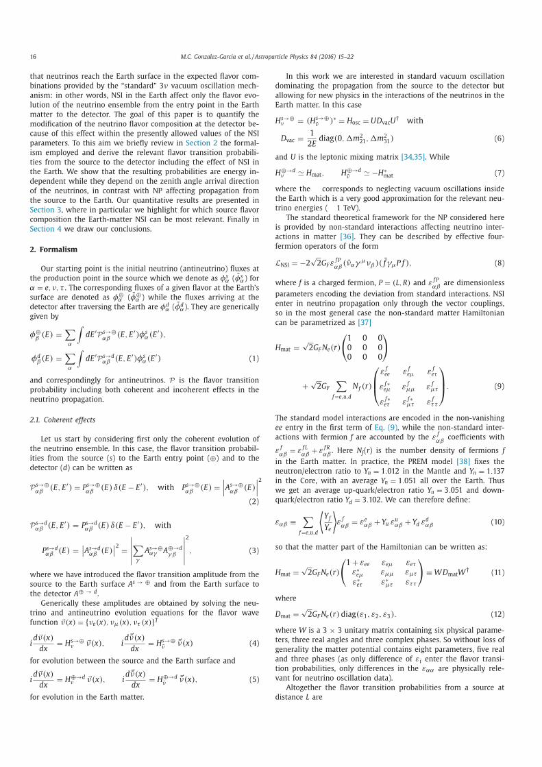
16 M.C. Gonzalez-Garcia et al. / Astroparticle Physics 84 (2016) 15–22
that neutrinos reach the Earth surface in the expected flavor com-
binations provided by the “standard” 3 ν vacuum oscillation mech-
anism: in other words, NSI in the Earth affect only the flavor evo-
lution of the neutrino ensemble from the entry point in the Earth
matter to the detector. The goal of this paper is to quantify the
modification of the neutrino flavor composition at the detector be-
cause of this effect within the presently allowed values of the NSI
parameters. To this aim we briefly review in Section 2 the formal-
ism employed and derive the relevant flavor transition probabili-
ties from the source to the detector including the effect of NSI in
the Earth. We show that the resulting probabilities are energy in-
dependent while they depend on the zenith angle arrival direction
of the neutrinos, in contrast with NP affecting propagation from
the source to the Earth. Our quantitative results are presented in
Section 3 , where in particular we highlight for which source flavor
composition the Earth-matter NSI can be most relevant. Finally in
Section 4 we draw our conclusions.
2. Formalism
Our starting point is the initial neutrino (antineutrino) fluxes at
the production point in the source which we denote as φs α ( φs
α) for
α = e, ν, τ . The corresponding fluxes of a given flavor at the Earth’s
surface are denoted as φ�α ( φ�
α ) while the fluxes arriving at the
detector after traversing the Earth are φd α ( φd
α). They are generically
given by
φ�
β(E) =
∑
α
∫ dE ′ P
s → �
αβ(E , E ′ ) φs
α(E ′ ) ,
φd β (E) =
∑
α
∫ dE ′ P
s → d αβ (E , E ′ ) φs
α(E ′ ) (1)
and correspondingly for antineutrinos. P is the flavor transition
probability including both coherent and incoherent effects in the
neutrino propagation.
2.1. Coherent effects
Let us start by considering first only the coherent evolution of
the neutrino ensemble. In this case, the flavor transition probabil-
ities from the source ( s ) to the Earth entry point ( �) and to the
detector ( d ) can be written as
P
s → �
αβ(E , E ′ ) = P s → �
αβ(E) δ(E − E ′ ) , with P s → �
αβ(E) =
∣∣∣A
s → �
αβ(E)
∣∣∣2
(2)
P
s → d αβ (E , E ′ ) = P s → d
αβ (E) δ(E − E ′ ) , with
P s → d αβ (E) =
∣∣A
s → d αβ (E)
∣∣2 =
∣∣∣∣∣∑
γ
A
s → �αγ A
�→ d γβ
∣∣∣∣∣2
, (3)
where we have introduced the flavor transition amplitude from the
source to the Earth surface A
s → � and from the Earth surface to
the detector A
� → d .
Generically these amplitudes are obtained by solving the neu-
trino and antineutrino evolution equations for the flavor wave
function
� ν(x ) = { νe (x ) , νμ(x ) , ντ (x ) } T
i d � ν(x )
dx = H
s → �ν �
ν(x ) , i d � ν(x )
dx = H
s → �
ν� ν(x ) (4)
for evolution between the source and the Earth surface and
i d � ν(x )
dx = H
�→ d ν �
ν(x ) , i d � ν(x )
dx = H
�→ d ν
� ν(x ) , (5)
for evolution in the Earth matter.
In this work we are interested in standard vacuum oscillation
dominating the propagation from the source to the detector but
allowing for new physics in the interactions of the neutrinos in the
Earth matter. In this case
H
s → �ν = (H
s → �
ν ) ∗ = H osc = U D vac U
† with
D vac =
1
2 E diag (0 , m
2 21 , m
2 31 ) (6)
and U is the leptonic mixing matrix [34,35] . While
H
�→ d ν � H mat , H
�→ d ν � −H
∗mat (7)
where the � corresponds to neglecting vacuum oscillations inside
the Earth which is a very good approximation for the relevant neu-
trino energies ( � 1 TeV).
The standard theoretical framework for the NP considered here
is provided by non-standard interactions affecting neutrino inter-
actions in matter [36] . They can be described by effective four-
fermion operators of the form
L NSI = −2
√
2 G F ε f P
αβ( ναγ μνβ )( f γμP f ) , (8)
where f is a charged fermion, P = (L, R ) and ε f P
αβare dimensionless
parameters encoding the deviation from standard interactions. NSI
enter in neutrino propagation only through the vector couplings,
so in the most general case the non-standard matter Hamiltonian
can be parametrized as [37]
H mat =
√
2 G F N e (r)
(
1 0 0
0 0 0
0 0 0
)
+
√
2 G F
∑
f= e,u,d
N f (r)
⎛
⎜ ⎝
ε f ee ε f eμ ε f eτ
ε f∗eμ ε f μμ ε f μτ
ε f∗eτ ε f∗μτ ε f ττ
⎞
⎟ ⎠
. (9)
The standard model interactions are encoded in the non-vanishing
ee entry in the first term of Eq. (9) , while the non-standard inter-
actions with fermion f are accounted by the ε f αβ
coefficients with
ε f αβ
= ε f L
αβ+ ε f R
αβ. Here N f ( r ) is the number density of fermions f
in the Earth matter. In practice, the PREM model [38] fixes the
neutron/electron ratio to Y n = 1 . 012 in the Mantle and Y n = 1 . 137
in the Core, with an average Y n = 1 . 051 all over the Earth. Thus
we get an average up-quark/electron ratio Y u = 3 . 051 and down-
quark/electron ratio Y d = 3 . 102 . We can therefore define:
ε αβ ≡∑
f= e,u,d
⟨Y f
Y e
⟩ε f αβ
= ε e αβ + Y u ε u αβ + Y d ε
d αβ (10)
so that the matter part of the Hamiltonian can be written as:
H mat =
√
2 G F N e (r)
(
1 + ε ee ε eμ ε eτε ∗eμ ε μμ ε μτ
ε ∗eτ ε ∗μτ ε ττ
)
≡ W D mat W
† (11)
where
D mat =
√
2 G F N e (r) diag (ε 1 , ε 2 , ε 3 ) . (12)
where W is a 3 × 3 unitary matrix containing six physical parame-
ters, three real angles and three complex phases. So without loss of
generality the matter potential contains eight parameters, five real
and three phases (as only difference of ε i enter the flavor transi-
tion probabilities, only differences in the ε αα are physically rele-
vant for neutrino oscillation data).
Altogether the flavor transition probabilities from a source at
distance L are
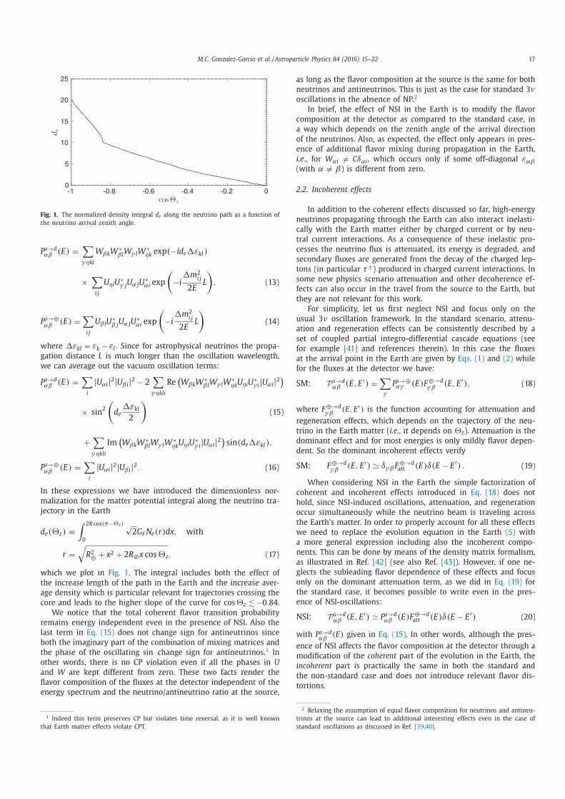
M.C. Gonzalez-Garcia et al. / Astroparticle Physics 84 (2016) 15–22 17
Fig. 1. The normalized density integral d e along the neutrino path as a function of
the neutrino arrival zenith angle.
P s → d αβ (E) =
∑
γ ηkl
W βk W
∗β l W γ l W
∗ηk exp (−id e ε kl )
×∑
i j
U ηi U
∗γ j U α j U
∗αi exp
(−i
m
2 i j
2 E L
), (13)
P s → �
αβ(E) =
∑
i j
U βi U
∗β j U α j U
∗αi exp
(−i
m
2 i j
2 E L
)(14)
where ε kl = ε k − ε l . Since for astrophysical neutrinos the propa-
gation distance L is much longer than the oscillation wavelength,
we can average out the vacuum oscillation terms:
P s → d αβ (E) =
∑
i
| U αi | 2 | U βi | 2 − 2
∑
γ ηkli
Re (W βk W
∗β l W γ l W
∗ηk U ηi U
∗γ i | U αi | 2
)
× sin
2
(d e
ε kl
2
)(15)
+
∑
γ ηkli
Im
(W βk W
∗β l W γ l W
∗ηk U ηi U
∗γ i | U αi | 2
)sin (d e ε kl ) ,
P s → �
αβ(E) =
∑
i
| U αi | 2 | U βi | 2 . (16)
In these expressions we have introduced the dimensionless nor-
malization for the matter potential integral along the neutrino tra-
jectory in the Earth
d e (�z ) ≡∫ 2 R cos (π−�z )
0
√
2 G F N e (r) dx, with
r =
√
R
2 �
+ x 2 + 2 R �x cos �z , (17)
which we plot in Fig. 1 . The integral includes both the effect of
the increase length of the path in the Earth and the increase aver-
age density which is particular relevant for trajectories crossing the
core and leads to the higher slope of the curve for cos �z � −0 . 84 .
We notice that the total coherent flavor transition probability
remains energy independent even in the presence of NSI. Also the
last term in Eq. (15) does not change sign for antineutrinos since
both the imaginary part of the combination of mixing matrices and
the phase of the oscillating sin change sign for antineutrinos. 1 In
other words, there is no CP violation even if all the phases in U
and W are kept different from zero. These two facts render the
flavor composition of the fluxes at the detector independent of the
energy spectrum and the neutrino/antineutrino ratio at the source,
1 Indeed this term preserves CP but violates time reversal, as it is well known
that Earth matter effects violate CPT.
as long as the flavor composition at the source is the same for both
neutrinos and antineutrinos. This is just as the case for standard 3 νoscillations in the absence of NP. 2
In brief, the effect of NSI in the Earth is to modify the flavor
composition at the detector as compared to the standard case, in
a way which depends on the zenith angle of the arrival direction
of the neutrinos. Also, as expected, the effect only appears in pres-
ence of additional flavor mixing during propagation in the Earth,
i.e. , for W αi � = C δαi , which occurs only if some off-diagonal ε αβ
(with α � = β) is different from zero.
2.2. Incoherent effects
In addition to the coherent effects discussed so far, high-energy
neutrinos propagating through the Earth can also interact inelasti-
cally with the Earth matter either by charged current or by neu-
tral current interactions. As a consequence of these inelastic pro-
cesses the neutrino flux is attenuated, its energy is degraded, and
secondary fluxes are generated from the decay of the charged lep-
tons (in particular τ±) produced in charged current interactions. In
some new physics scenario attenuation and other decoherence ef-
fects can also occur in the travel from the source to the Earth, but
they are not relevant for this work.
For simplicity, let us first neglect NSI and focus only on the
usual 3 ν oscillation framework. In the standard scenario, attenu-
ation and regeneration effects can be consistently described by a
set of coupled partial integro-differential cascade equations (see
for example [41] and references therein). In this case the fluxes
at the arrival point in the Earth are given by Eqs. (1) and (2) while
for the fluxes at the detector we have:
SM: P
s → d αβ (E , E ′ ) =
∑
γ
P s → �αγ (E ) F �→ d
γβ(E , E ′ ) , (18)
where F �→ d γ β
(E , E ′ ) is the function accounting for attenuation and
regeneration effects, which depends on the trajectory of the neu-
trino in the Earth matter ( i.e. , it depends on �z ). Attenuation is the
dominant effect and for most energies is only mildly flavor depen-
dent. So the dominant incoherent effects verify
SM: F �→ d γ β
(E , E ′ ) � δγβF �→ d att (E) δ(E − E ′ ) . (19)
When considering NSI in the Earth the simple factorization of
coherent and incoherent effects introduced in Eq. (18) does not
hold, since NSI-induced oscillations, attenuation, and regeneration
occur simultaneously while the neutrino beam is traveling across
the Earth’s matter. In order to properly account for all these effects
we need to replace the evolution equation in the Earth (5) with
a more general expression including also the incoherent compo-
nents. This can be done by means of the density matrix formalism,
as illustrated in Ref. [42] (see also Ref. [43] ). However, if one ne-
glects the subleading flavor dependence of these effects and focus
only on the dominant attenuation term, as we did in Eq. (19) for
the standard case, it becomes possible to write even in the pres-
ence of NSI-oscillations:
NSI: P
s → d αβ (E , E ′ ) � P s → d
αβ (E ) F �→ d att (E ) δ(E − E ′ ) (20)
with P s → d αβ
(E) given in Eq. (15) . In other words, although the pres-
ence of NSI affects the flavor composition at the detector through a
modification of the coherent part of the evolution in the Earth, the
incoherent part is practically the same in both the standard and
the non-standard case and does not introduce relevant flavor dis-
tortions.
2 Relaxing the assumption of equal flavor composition for neutrinos and antineu-
trinos at the source can lead to additional interesting effects even in the case of
standard oscillations as discussed in Ref. [39,40] .
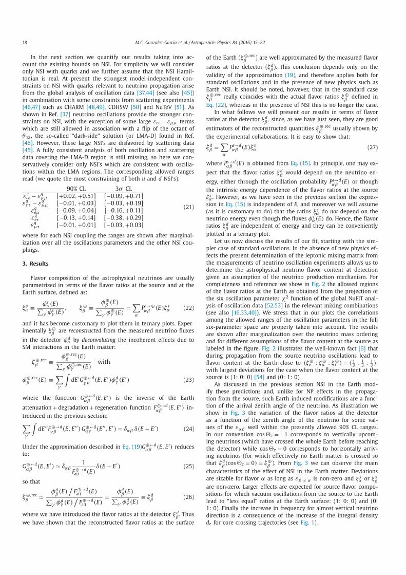
18 M.C. Gonzalez-Garcia et al. / Astroparticle Physics 84 (2016) 15–22
In the next section we quantify our results taking into ac-
count the existing bounds on NSI. For simplicity we will consider
only NSI with quarks and we further assume that the NSI Hamil-
tonian is real. At present the strongest model-independent con-
straints on NSI with quarks relevant to neutrino propagation arise
from the global analysis of oscillation data [37,44] (see also [45] )
in combination with some constraints from scattering experiments
[46,47] such as CHARM [4 8,4 9] , CDHSW [50] and NuTeV [51] . As
shown in Ref. [37] neutrino oscillations provide the stronger con-
straints on NSI, with the exception of some large ε ee − ε μμ terms
which are still allowed in association with a flip of the octant of
θ12 , the so-called “dark-side” solution (or LMA-D) found in Ref.
[45] . However, these large NSI’s are disfavored by scattering data
[45] . A fully consistent analysis of both oscillation and scattering
data covering the LMA-D region is still missing, so here we con-
servatively consider only NSI’s which are consistent with oscilla-
tions within the LMA regions. The corresponding allowed ranges
read (we quote the most constraining of both u and d NSI’s):
90% CL 3 σ CL
ε q ee − ε q μμ [+0 . 02 , +0 . 51] [ −0 . 09 , +0 . 71]
ε q ττ − ε q μμ [ −0 . 01 , +0 . 03] [ −0 . 03 , +0 . 19]
ε q eμ [ −0 . 09 , +0 . 04] [ −0 . 16 , +0 . 11]
ε q eτ [ −0 . 13 , +0 . 14] [ −0 . 38 , +0 . 29]
ε q μτ [ −0 . 01 , +0 . 01] [ −0 . 03 , +0 . 03]
(21)
where for each NSI coupling the ranges are shown after marginal-
ization over all the oscillations parameters and the other NSI cou-
plings.
3. Results
Flavor composition of the astrophysical neutrinos are usually
parametrized in terms of the flavor ratios at the source and at the
Earth surface, defined as:
ξ s α ≡ φs
α(E) ∑
γ φs γ (E)
, ξ�
β≡
φ�
β(E) ∑
γ φ�γ (E)
=
∑
α
P s → �
αβ(E) ξ s
α (22)
and it has become customary to plot them in ternary plots. Exper-
imentally ξ�
βare reconstructed from the measured neutrino fluxes
in the detector φd α by deconvoluting the incoherent effects due to
SM interactions in the Earth matter:
ξ�, rec β
≡φ�, rec
β(E) ∑
γ φ�, rec γ (E)
with
φ�, rec β
(E) ≡∑
γ
∫ dE ′ G
�← d γ β
(E , E ′ ) φd γ (E ′ ) (23)
where the function G
�← d αβ
(E , E ′ ) is the inverse of the Earth
attenuation + degradation + regeneration function F �→ d αβ
(E , E ′ ) in-
troduced in the previous section: ∑
γ
∫ dE ′′ F �→ d
γ β(E , E ′′ ) G
�← d αγ (E ′′ , E ′ ) = δαβ δ(E − E ′ ) (24)
Under the approximation described in Eq. (19) G
�← d αβ
(E , E ′ ) reduces
to:
G
�← d αβ
(E , E ′ ) � δαβ1
F �→ d att (E)
δ(E − E ′ ) (25)
so that
ξ�, rec β
�
φd β(E)
/F �→ d
att (E) ∑
γ φd γ (E)
/F �→ d
att (E) =
φd β(E) ∑
γ φd γ (E)
≡ ξ d β (26)
where we have introduced the flavor ratios at the detector ξ d β
. Thus
we have shown that the reconstructed flavor ratios at the surface
of the Earth ( ξ�, rec β
) are well approximated by the measured flavor
ratios at the detector ( ξ d β
). This conclusion depends only on the
validity of the approximation (19) , and therefore applies both for
standard oscillations and in the presence of new physics such as
Earth NSI. It should be noted, however, that in the standard case
ξ�, rec β
really coincides with the actual flavor ratios ξ�
βdefined in
Eq. (22) , whereas in the presence of NSI this is no longer the case.
In what follows we will present our results in terms of flavor
ratios at the detector ξ d β, since, as we have just seen, they are good
estimators of the reconstructed quantities ξ�, rec β
usually shown by
the experimental collaborations. It is easy to show that:
ξ d β =
∑
α
P s → d αβ (E) ξ s
α (27)
where P s → d αβ
(E) is obtained from Eq. (15) . In principle, one may ex-
pect that the flavor ratios ξ d β
would depend on the neutrino en-
ergy, either through the oscillation probability P s → d αβ
(E) or though
the intrinsic energy dependence of the flavor ratios at the source
ξ s α . However, as we have seen in the previous section the expres-
sion in Eq. (15) is independent of E , and moreover we will assume
(as it is customary to do) that the ratios ξ s α do not depend on the
neutrino energy even though the fluxes φs α(E) do. Hence, the flavor
ratios ξ d β
are independent of energy and they can be conveniently
plotted in a ternary plot.
Let us now discuss the results of our fit, starting with the sim-
pler case of standard oscillations. In the absence of new physics ef-
fects the present determination of the leptonic mixing matrix from
the measurements of neutrino oscillation experiments allows us to
determine the astrophysical neutrino flavor content at detection
given an assumption of the neutrino production mechanism. For
completeness and reference we show in Fig. 2 the allowed regions
of the flavor ratios at the Earth as obtained from the projection of
the six oscillation parameter χ2 function of the global NuFIT anal-
ysis of oscillation data [52,53] in the relevant mixing combinations
(see also [16,33,40] ). We stress that in our plots the correlations
among the allowed ranges of the oscillation parameters in the full
six-parameter space are properly taken into account. The results
are shown after marginalization over the neutrino mass ordering
and for different assumptions of the flavor content at the source as
labeled in the figure. Fig. 2 illustrates the well-known fact [6] that
during propagation from the source neutrino oscillations lead to
flavor content at the Earth close to (ξ�e : ξ�
μ : ξ�τ ) = ( 1 3 : 1
3 : 1 3 ) ,
with largest deviations for the case when the flavor content at the
source is (1: 0: 0) [54] and (0: 1: 0).
As discussed in the previous section NSI in the Earth mod-
ify these predictions and, unlike for NP effects in the propaga-
tion from the source, such Earth-induced modifications are a func-
tion of the arrival zenith angle of the neutrino. As illustration we
show in Fig. 3 the variation of the flavor ratios at the detector
as a function of the zenith angle of the neutrino for some val-
ues of the ε αβ well within the presently allowed 90% CL ranges.
In our convention cos �z = −1 corresponds to vertically upcom-
ing neutrinos (which have crossed the whole Earth before reaching
the detector) while cos �z = 0 corresponds to horizontally arriv-
ing neutrinos (for which effectively no Earth matter is crossed so
that ξ d β( cos �z = 0) = ξ�
β). From Fig. 3 we can observe the main
characteristics of the effect of NSI in the Earth matter. Deviations
are sizable for flavor α as long as ε β � = α is non-zero and ξ s α or ξ s
β
are non-zero. Larger effects are expected for source flavor compo-
sitions for which vacuum oscillations from the source to the Earth
lead to “less equal” ratios at the Earth surface: (1: 0: 0) and (0:
1: 0). Finally the increase in frequency for almost vertical neutrino
direction is a consequence of the increase of the integral density
d e for core crossing trajectories (see Fig. 1 ).
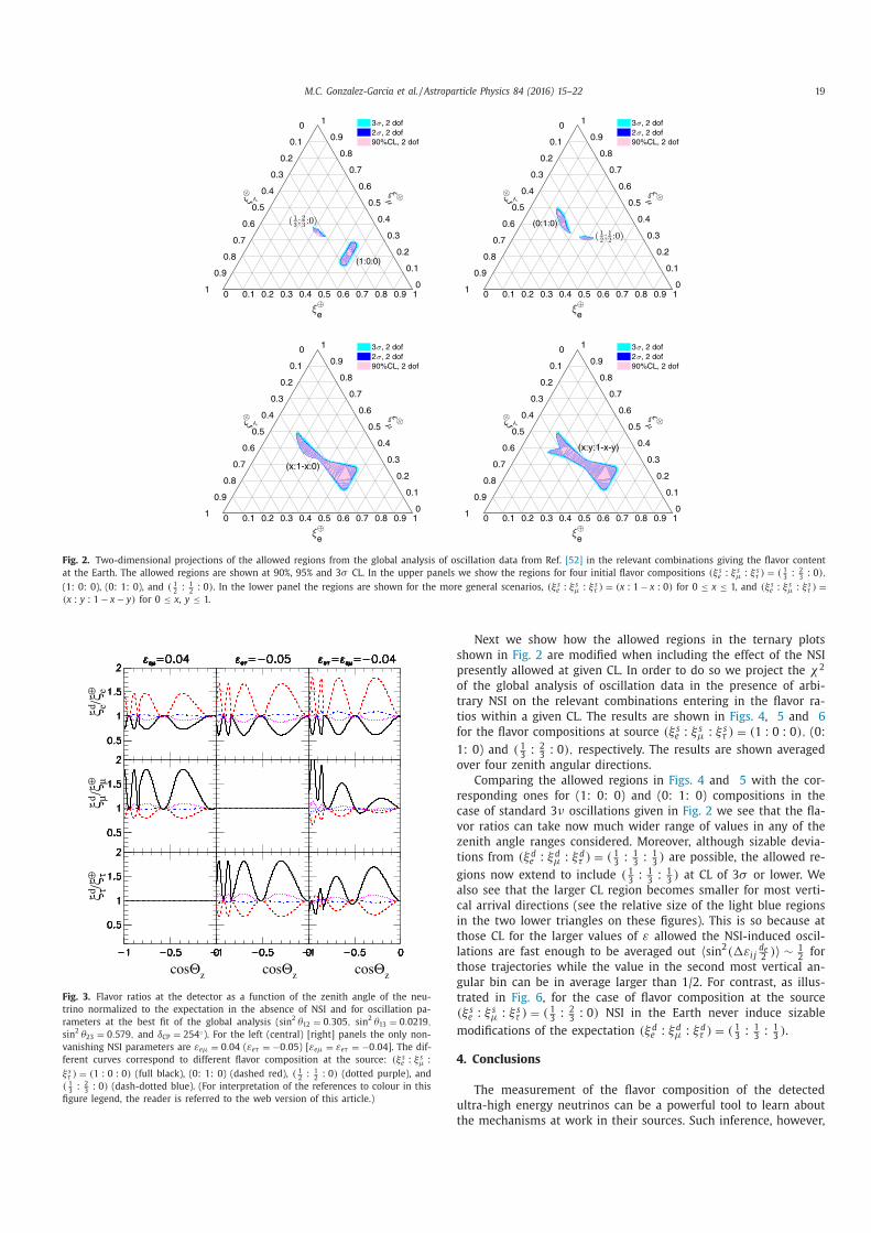
M.C. Gonzalez-Garcia et al. / Astroparticle Physics 84 (2016) 15–22 19
Fig. 2. Two-dimensional projections of the allowed regions from the global analysis of oscillation data from Ref. [52] in the relevant combinations giving the flavor content
at the Earth. The allowed regions are shown at 90%, 95% and 3 σ CL. In the upper panels we show the regions for four initial flavor compositions (ξ s e : ξ
s μ : ξ s
τ ) = ( 1 3
: 2 3
: 0) ,
(1: 0: 0), (0: 1: 0), and ( 1 2
: 1 2
: 0) . In the lower panel the regions are shown for the more general scenarios, (ξ s e : ξ
s μ : ξ s
τ ) = (x : 1 − x : 0) for 0 ≤ x ≤ 1, and (ξ s e : ξ
s μ : ξ s
τ ) =
(x : y : 1 − x − y ) for 0 ≤ x , y ≤ 1.
ξ ed/ξe⊕
ξ μd /ξ μ⊕
ξ τd /ξ τ⊕
cosΘz cosΘz cosΘz
Fig. 3. Flavor ratios at the detector as a function of the zenith angle of the neu-
trino normalized to the expectation in the absence of NSI and for oscillation pa-
rameters at the best fit of the global analysis ( sin 2 θ12 = 0 . 305 , sin
2 θ13 = 0 . 0219 ,
sin 2 θ23 = 0 . 579 , and δCP = 254 ◦). For the left (central) [right] panels the only non-
vanishing NSI parameters are ε eμ = 0 . 04 ( ε eτ = −0 . 05 ) [ ε eμ = ε eτ = −0 . 04 ]. The dif-
ferent curves correspond to different flavor composition at the source: (ξ s e : ξ
s μ :
ξ s τ ) = (1 : 0 : 0) (full black), (0: 1: 0) (dashed red), ( 1
2 : 1
2 : 0) (dotted purple), and
( 1 3
: 2 3
: 0) (dash-dotted blue). (For interpretation of the references to colour in this
figure legend, the reader is referred to the web version of this article.)
Next we show how the allowed regions in the ternary plots
shown in Fig. 2 are modified when including the effect of the NSI
presently allowed at given CL. In order to do so we project the χ2
of the global analysis of oscillation data in the presence of arbi-
trary NSI on the relevant combinations entering in the flavor ra-
tios within a given CL. The results are shown in Figs. 4 , 5 and 6
for the flavor compositions at source (ξ s e : ξ s
μ : ξ s τ ) = (1 : 0 : 0) , (0:
1: 0) and ( 1 3 : 2 3 : 0) , respectively. The results are shown averaged
over four zenith angular directions.
Comparing the allowed regions in Figs. 4 and 5 with the cor-
responding ones for (1: 0: 0) and (0: 1: 0) compositions in the
case of standard 3 ν oscillations given in Fig. 2 we see that the fla-
vor ratios can take now much wider range of values in any of the
zenith angle ranges considered. Moreover, although sizable devia-
tions from (ξ d e : ξ d
μ : ξ d τ ) = ( 1 3 : 1
3 : 1 3 ) are possible, the allowed re-
gions now extend to include ( 1 3 : 1 3 : 1
3 ) at CL of 3 σ or lower. We
also see that the larger CL region becomes smaller for most verti-
cal arrival directions (see the relative size of the light blue regions
in the two lower triangles on these figures). This is so because at
those CL for the larger values of ε allowed the NSI-induced oscil-
lations are fast enough to be averaged out 〈 sin
2 (ε i j d e 2 ) 〉 ∼ 1
2 for
those trajectories while the value in the second most vertical an-
gular bin can be in average larger than 1/2. For contrast, as illus-
trated in Fig. 6 , for the case of flavor composition at the source
(ξ s e : ξ s
μ : ξ s τ ) = ( 1 3 : 2
3 : 0) NSI in the Earth never induce sizable
modifications of the expectation (ξ d e : ξ d
μ : ξ d τ ) = ( 1 3 : 1
3 : 1 3 ) .
4. Conclusions
The measurement of the flavor composition of the detected
ultra-high energy neutrinos can be a powerful tool to learn about
the mechanisms at work in their sources. Such inference, however,

20 M.C. Gonzalez-Garcia et al. / Astroparticle Physics 84 (2016) 15–22
Fig. 4. Allowed regions for the flavor ratios in the presence of NSI in the Earth at 90, 95% and 3 σ CL for an initial flavor (ξ s e : ξ
s μ : ξ s
τ ) = (1 : 0 : 0) . The four triangles
correspond to averaging over neutrinos arriving with directions given in the range 0 ≥ cos �z > −0 . 25 (upper left), −0 . 25 ≥ cos �z > −0 . 5 (upper right) −0 . 5 ≥ cos �z >
−0 . 75 (lower left), and −0 . 75 ≥ cos �z ≥ −1 (lower right).
Fig. 5. Same as Fig. 4 for (ξ s e : ξ
s μ : ξ s
τ ) = (0 : 1 : 0) .
relies on the understanding of the particle physics processes rele-
vant to the neutrino propagation from the source to the detector.
The presence of NP effects beyond those of the well established
mass-induced 3 ν oscillations alter the flavor composition at the
detector and can therefore affect the conclusions on the dominant
production mechanism.
In this work we have focused on NP effects associated with NSI
of the neutrinos in the Earth matter. The relevant flavor transition
probabilities accounting from oscillations from the source to the
Earth plus NSI in the Earth are energy independent but depend on
the zenith angle of the arrival direction of the neutrinos, which is
a characteristic feature of this form of NP. Quantitatively, we have
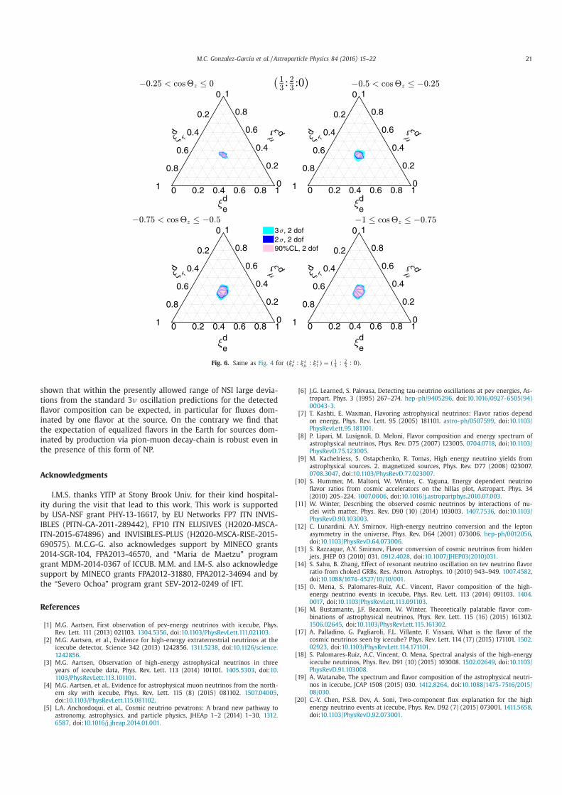
M.C. Gonzalez-Garcia et al. / Astroparticle Physics 84 (2016) 15–22 21
Fig. 6. Same as Fig. 4 for (ξ s e : ξ
s μ : ξ s
τ ) = ( 1 3
: 2 3
: 0) .
shown that within the presently allowed range of NSI large devia-
tions from the standard 3 ν oscillation predictions for the detected
flavor composition can be expected, in particular for fluxes dom-
inated by one flavor at the source. On the contrary we find that
the expectation of equalized flavors in the Earth for sources dom-
inated by production via pion-muon decay-chain is robust even in
the presence of this form of NP.
Acknowledgments
I.M.S. thanks YITP at Stony Brook Univ. for their kind hospital-
ity during the visit that lead to this work. This work is supported
by USA-NSF grant PHY-13-16617, by EU Networks FP7 ITN INVIS-
IBLES (PITN-GA-2011-289442), FP10 ITN ELUSIVES (H2020-MSCA-
ITN-2015-674896) and INVISIBLES-PLUS (H2020-MSCA-RISE-2015-
690575). M.C.G-G. also acknowledges support by MINECO grants
2014-SGR-104, FPA2013-46570, and “Maria de Maetzu” program
grant MDM-2014-0367 of ICCUB. M.M. and I.M-S. also acknowledge
support by MINECO grants FPA2012-31880, FPA2012-34694 and by
the “Severo Ochoa” program grant SEV-2012-0249 of IFT.
References
[1] M.G. Aartsen, First observation of pev-energy neutrinos with icecube, Phys. Rev. Lett. 111 (2013) 021103. 1304.5356 , doi: 10.1103/PhysRevLett.111.021103 .
[2] M.G. Aartsen, et al., Evidence for high-energy extraterrestrial neutrinos at the icecube detector, Science 342 (2013) 1242856. 1311.5238 , doi: 10.1126/science.
1242856 . [3] M.G. Aartsen, Observation of high-energy astrophysical neutrinos in three
years of icecube data, Phys. Rev. Lett. 113 (2014) 101101. 1405.5303 , doi: 10. 1103/PhysRevLett.113.101101 .
[4] M.G. Aartsen, et al., Evidence for astrophysical muon neutrinos from the north-
ern sky with icecube, Phys. Rev. Lett. 115 (8) (2015) 081102. 1507.04005 , doi: 10.1103/PhysRevLett.115.081102 .
[5] L.A. Anchordoqui, et al., Cosmic neutrino pevatrons: A brand new pathway to astronomy, astrophysics, and particle physics, JHEAp 1–2 (2014) 1–30. 1312.
6587 , doi: 10.1016/j.jheap.2014.01.001 .
[6] J.G. Learned, S. Pakvasa, Detecting tau-neutrino oscillations at pev energies, As-
tropart. Phys. 3 (1995) 267–274. hep-ph/9405296 , doi: 10.1016/0927-6505(94) 0 0 043-3 .
[7] T. Kashti, E. Waxman, Flavoring astrophysical neutrinos: Flavor ratios depend on energy, Phys. Rev. Lett. 95 (2005) 181101. astro-ph/0507599 , doi: 10.1103/
PhysRevLett.95.181101 .
[8] P. Lipari, M. Lusignoli, D. Meloni, Flavor composition and energy spectrum of astrophysical neutrinos, Phys. Rev. D75 (2007) 123005. 0704.0718 , doi: 10.1103/
PhysRevD.75.123005 . [9] M. Kachelriess, S. Ostapchenko, R. Tomas, High energy neutrino yields from
astrophysical sources. 2. magnetized sources, Phys. Rev. D77 (20 08) 0230 07. 0708.3047 , doi: 10.1103/PhysRevD.77.023007 .
[10] S. Hummer, M. Maltoni, W. Winter, C. Yaguna, Energy dependent neutrino
flavor ratios from cosmic accelerators on the hillas plot, Astropart. Phys. 34 (2010) 205–224. 10 07.0 0 06 , doi: 10.1016/j.astropartphys.2010.07.003 .
[11] W. Winter, Describing the observed cosmic neutrinos by interactions of nu- clei with matter, Phys. Rev. D90 (10) (2014) 103003. 1407.7536 , doi: 10.1103/
PhysRevD.90.103003 . [12] C. Lunardini, A.Y. Smirnov, High-energy neutrino conversion and the lepton
asymmetry in the universe, Phys. Rev. D64 (20 01) 0730 06. hep-ph/0 012056 ,
doi: 10.1103/PhysRevD.64.073006 . [13] S. Razzaque, A.Y. Smirnov, Flavor conversion of cosmic neutrinos from hidden
jets, JHEP 03 (2010) 031. 0912.4028 , doi: 10.1007/JHEP03(2010)031 . [14] S. Sahu, B. Zhang, Effect of resonant neutrino oscillation on tev neutrino flavor
ratio from choked GRBs, Res. Astron. Astrophys. 10 (2010) 943–949. 1007.4582 , doi: 10.1088/1674-4527/10/10/001 .
[15] O. Mena, S. Palomares-Ruiz, A.C. Vincent, Flavor composition of the high-
energy neutrino events in icecube, Phys. Rev. Lett. 113 (2014) 091103. 1404. 0017 , doi: 10.1103/PhysRevLett.113.091103 .
[16] M. Bustamante, J.F. Beacom, W. Winter, Theoretically palatable flavor com- binations of astrophysical neutrinos, Phys. Rev. Lett. 115 (16) (2015) 161302.
1506.02645 , doi: 10.1103/PhysRevLett.115.161302 . [17] A. Palladino, G. Pagliaroli, F.L. Villante, F. Vissani, What is the flavor of the
cosmic neutrinos seen by icecube? Phys. Rev. Lett. 114 (17) (2015) 171101. 1502.
02923 , doi: 10.1103/PhysRevLett.114.171101 . [18] S. Palomares-Ruiz, A.C. Vincent, O. Mena, Spectral analysis of the high-energy
icecube neutrinos, Phys. Rev. D91 (10) (2015) 103008. 1502.02649 , doi: 10.1103/ PhysRevD.91.103008 .
[19] A. Watanabe, The spectrum and flavor composition of the astrophysical neutri- nos in icecube, JCAP 1508 (2015) 030. 1412.8264 , doi: 10.1088/1475-7516/2015/
08/030 . [20] C.-Y. Chen, P.S.B. Dev, A. Soni, Two-component flux explanation for the high
energy neutrino events at icecube, Phys. Rev. D92 (7) (2015) 073001. 1411.5658 ,
doi: 10.1103/PhysRevD.92.073001 .
22 M.C. Gonzalez-Garcia et al. / Astroparticle Physics 84 (2016) 15–22
[21] N. Kawanaka, K. Ioka, Neutrino flavor ratios modified by cosmic ray sec- ondary acceleration, Phys. Rev. D92 (8) (2015) 085047. 1504.03417 , doi: 10.1103/
PhysRevD.92.085047 . [22] M.G. Aartsen, et al., A combined maximum-likelihood analysis of the high-
energy astrophysical neutrino flux measured with icecube, Astrophys. J. 809 (1) (2015) 98. 1507.03991 , doi: 10.1088/0 0 04-637X/809/1/98 .
[23] A.C. Vincent, S. Palomares-Ruiz, O. Mena, Analysis of the 4-year icecube HESE data, (2016). arXiv:1605.01556 .
[24] D. Hooper, D. Morgan, E. Winstanley, Lorentz and CPT invariance violation in
high-energy neutrinos, Phys. Rev. D72 (2005) 065009. hep-ph/0506091 , doi: 10. 1103/PhysRevD.72.065009 .
[25] J.F. Beacom, N.F. Bell, D. Hooper, S. Pakvasa, T.J. Weiler, Decay of high-energy astrophysical neutrinos, Phys. Rev. Lett. 90 (2003) 181301. hep-ph/0211305 ,
doi: 10.1103/PhysRevLett.90.181301 . [26] P. Baerwald, M. Bustamante, W. Winter, Neutrino decays over cosmological
distances and the implications for neutrino telescopes, JCAP 1210 (2012) 020.
1208.4600 , doi: 10.1088/1475-7516/2012/10/020 . [27] L.A. Anchordoqui, H. Goldberg, M.C. Gonzalez-Garcia, F. Halzen, D. Hooper,
S. Sarkar, T.J. Weiler, Probing planck scale physics with icecube, Phys. Rev. D72 (2005) 065019. hep-ph/0506168 , doi: 10.1103/PhysRevD.72.065019 .
[28] D. Hooper, D. Morgan, E. Winstanley, Probing quantum decoherence with high- energy neutrinos, Phys. Lett. B609 (2005) 206–211. hep-ph/0410094 , doi: 10.
1016/j.physletb.2005.01.034 .
[29] J.F. Beacom, N.F. Bell, D. Hooper, J.G. Learned, S. Pakvasa, T.J. Weiler, Pseu- dodirac neutrinos: A challenge for neutrino telescopes, Phys. Rev. Lett. 92
(2004) 011101. hep-ph/0307151 , doi: 10.1103/PhysRevLett.92.011101 . [30] A. Esmaili, Pseudo-dirac neutrino scenario: Cosmic neutrinos at neutrino tele-
scopes, Phys. Rev. D81 (2010) 013006. 0909.5410 , doi: 10.1103/PhysRevD.81. 013006 .
[31] H. Athar, M. Jezabek, O. Yasuda, Effects of neutrino mixing on high-energy cos-
mic neutrino flux, Phys. Rev. D62 (20 0 0) 1030 07. hep-ph/0 0 05104 , doi: 10.1103/ PhysRevD.62.103007 .
[32] P.F. de Salas, R.A. Lineros, M. Tórtola, Neutrino propagation in the galactic dark matter halo, (2016). arXiv:1601.05798 .
[33] C.A. Argüelles, T. Katori, J. Salvado, New physics in astrophysical neutrino fla- vor, Phys. Rev. Lett. 115 (2015) 161303. 1506.02043 , doi: 10.1103/PhysRevLett.
115.161303 .
[34] Z. Maki, M. Nakagawa, S. Sakata, Remarks on the unified model of elementary particles, Prog. Theor. Phys. 28 (1962) 870–880, doi: 10.1143/PTP.28.870 .
[35] M. Kobayashi, T. Maskawa, CP violation in the renormalizable theory of weak interaction, Prog. Theor. Phys. 49 (1973) 652–657, doi: 10.1143/PTP.49.652 .
[36] L. Wolfenstein, Neutrino oscillations in matter, Phys. Rev. D17 (1978) 2369–2374, doi: 10.1103/PhysRevD.17.2369 .
[37] M.C. Gonzalez-Garcia, M. Maltoni, Determination of matter potential from
global analysis of neutrino oscillation data, JHEP 09 (2013) 152. 1307.3092 , doi: 10.1007/JHEP09(2013)152 .
[38] A. Dziewonski, D. Anderson, Preliminary reference earth model, Phys. Earth Planet. Interiors 25 (1981) 297–356, doi: 10.1016/0031-9201(81)90046-7 .
[39] I.M. Shoemaker, K. Murase, Probing BSM neutrino physics with flavor and spectral distortions: Prospects for future high-energy neutrino telescopes,
Phys. Rev. D93 (8) (2016) 085004. 1512.07228 , doi: 10.1103/PhysRevD.93. 085004 .
[40] H. Nunokawa, B. Panes, R.Z. Funchal, How unequal fluxes of high energy as- trophysical neutrinos and antineutrinos can fake new physics, (2016). arXiv:
1604.08595. [41] J. Jones, I. Mocioiu, M.H. Reno, I. Sarcevic, Tracing very high-energy neu-
trinos from cosmological distances in ice, Phys. Rev. D69 (2004) 033004.
hep-ph/0308042 , doi: 10.1103/PhysRevD.69.033004 . [42] M.C. Gonzalez-Garcia, F. Halzen, M. Maltoni, Physics reach of high-energy
and high-statistics icecube atmospheric neutrino data, Phys. Rev. D71 (2005) 093010. hep-ph/0502223 , doi: 10.1103/PhysRevD.71.093010 .
[43] C.A .A . Delgado, J. Salvado, C.N. Weaver, A simple quantum integro-differential solver (SQuIDS), Comput. Phys. Commun. 196 (2015) 569–591. 1412.3832 ,
doi: 10.1016/j.cpc.2015.06.022 .
[44] M.C. Gonzalez-Garcia, M. Maltoni, J. Salvado, Testing matter effects in propa- gation of atmospheric and long-baseline neutrinos, JHEP 05 (2011) 075. 1103.
4365 , doi: 10.1007/JHEP05(2011)075 . [45] O. Miranda, M. Tórtola, J. Valle, Are solar neutrino oscillations robust? JHEP
0610 (2006) 008. hep-ph/0406280 , doi: 10.1088/1126-6708/2006/10/008 . [46] S. Davidson, C. Pena-Garay, N. Rius, A. Santamaria, Present and future bounds
on nonstandard neutrino interactions, JHEP 0303 (2003) 011. hep-ph/0302093 .
[47] C. Biggio, M. Blennow, E. Fernandez-Martinez, General bounds on non- standard neutrino interactions, JHEP 0908 (20 09) 090. 0907.0 097 , doi: 10.1088/
1126-6708/2009/08/090 . [48] J. Dorenbosch, et al., Experimental verification of the universality of electron-
neutrino and muon-neutrino coupling to the neutral weak current, Phys. Lett. B180 (1986) 303, doi: 10.1016/0370-2693(86)90315-1 .
[49] J. Allaby, et al., A precise determination of the electroweak mixing angle
from semileptonic neutrino scattering, Z. Phys. C36 (1987) 611, doi: 10.1007/ BF01630598 .
[50] A. Blondel, P. Bockmann, H. Burkhardt, F. Dydak, A. Grant, et al., Electroweak parameters from a high statistics neutrino nucleon scattering experiment,
Z.Phys. C45 (1990) 361–379, doi: 10.1007/BF01549665 . [51] G. Zeller, et al., A precise determination of electroweak parameters in neutrino
nucleon scattering, Phys. Rev. Lett. 88 (2002) 091802. hep-ex/0110059 , doi: 10.
1103/PhysRevLett.88.091802 . [52] M.C. Gonzalez-Garcia, M. Maltoni, T. Schwetz, Updated fit to three neutrino
mixing: status of leptonic CP violation, JHEP 11 (2014) 052. 1409.5439 , doi: 10. 1007/JHEP11(2014)052 .
[53] M. Gonzalez-Garcia, M. Maltoni, T. Schwetz, Nufit 2.0, 2014, http://www.nu-fit. org .
[54] A. Palladino, F. Vissani, The natural parameterization of cosmic neutrino
oscillations, Eur. Phys. J. C75 (2015) 433. 1504.05238 , doi: 10.1140/epjc/ s10052-015-3664-6 .

CHAPTER 4. NSI AND ASTROPHYSICAL NEUTRINOS
86
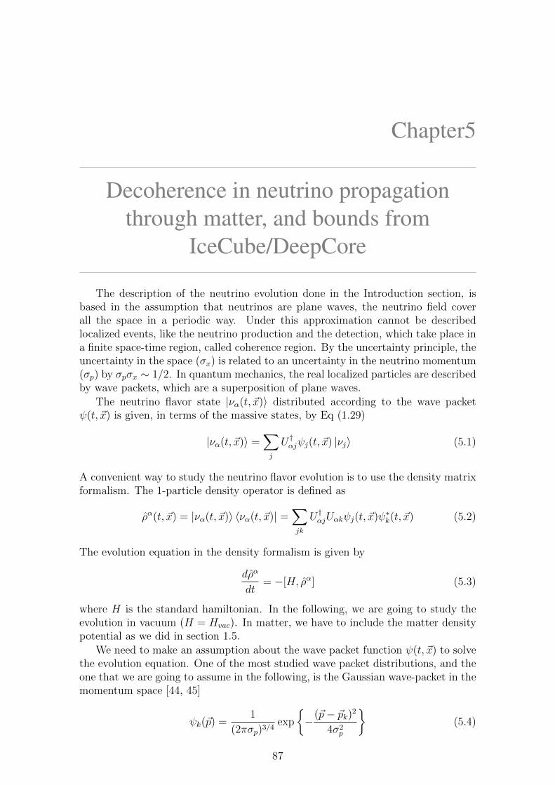
Chapter5
Decoherence in neutrino propagationthrough matter, and bounds from
IceCube/DeepCore
The description of the neutrino evolution done in the Introduction section, isbased in the assumption that neutrinos are plane waves, the neutrino field coverall the space in a periodic way. Under this approximation cannot be describedlocalized events, like the neutrino production and the detection, which take place ina finite space-time region, called coherence region. By the uncertainty principle, theuncertainty in the space (σx) is related to an uncertainty in the neutrino momentum(σp) by σpσx ∼ 1/2. In quantum mechanics, the real localized particles are describedby wave packets, which are a superposition of plane waves.
The neutrino flavor state |να(t, ~x)〉 distributed according to the wave packetψ(t, ~x) is given, in terms of the massive states, by Eq (1.29)
|να(t, ~x)〉 =∑
j
U †αjψj(t, ~x) |νj〉 (5.1)
A convenient way to study the neutrino flavor evolution is to use the density matrixformalism. The 1-particle density operator is defined as
ρα(t, ~x) = |να(t, ~x)〉 〈να(t, ~x)| =∑
jk
U †αjUαkψj(t, ~x)ψ∗k(t, ~x) (5.2)
The evolution equation in the density formalism is given by
dρα
dt= −[H, ρα] (5.3)
where H is the standard hamiltonian. In the following, we are going to study theevolution in vacuum (H = Hvac). In matter, we have to include the matter densitypotential as we did in section 1.5.
We need to make an assumption about the wave packet function ψ(t, ~x) to solvethe evolution equation. One of the most studied wave packet distributions, and theone that we are going to assume in the following, is the Gaussian wave-packet in themomentum space [44, 45]
ψk(~p) =1
(2πσp)3/4exp
{−(~p− ~pk)2
4σ2p
}(5.4)
87
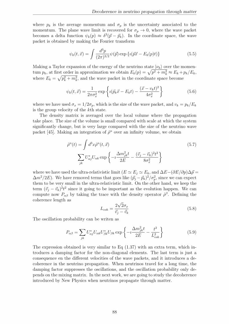
Decoherence in neutrino propagation through matter
where pk is the average momentum and σp is the uncertainty associated to themomentum. The plane wave limit is recovered for σp → 0, where the wave packetbecomes a delta function ψk(p) ≈ δ3(~p − ~pk). In the coordinate space, the wavepacket is obtained by making the Fourier transform
ψk(t, ~x) =
∫d3p
(2π)3/2ψ(~p) exp {ı(~p~x− Ek(p)t)} (5.5)
Making a Taylor expansion of the energy of the neutrino state |νk〉 over the momen-tum pk, at first order in approximation we obtain Ek(p) =
√p2 +m2
k ≈ Ek +pk/Ek,
where Ek =√p2k +m2
k, and the wave packet in the coordinate space become
ψk(t, ~x) =1
2πσ2x
exp
{ı(~pk~x− Ekt)−
(~x− vkt)2
4σ2x
}(5.6)
where we have used σx = 1/2σp, which is the size of the wave packet, and vk = pk/Ekis the group velocity of the kth state.
The density matrix is averaged over the local volume where the propagationtake place. The size of the volume is small compared with scale at which the systemsignificantly change, but is very large compared with the size of the neutrino wavepacket [45]. Making an integration of ρα over an infinity volume, we obtain
ρα(t) =
∫d3xρα(t, ~x) (5.7)
∑
jk
U∗αjUαk exp
{−ı
∆m2jkt
2E− (~vj − ~vk)2t2
8σ2x
}
where we have used the ultra-relativistic limit (E ' Ej ' Ek, and ∆E−(∂E/∂p)∆~p =∆m2/2E). We have removed terms that goes like (~pj−~pk)2/σ2
p, since we can expectthem to be very small in the ultra-relativistic limit. On the other hand, we keep theterm (~vj − ~vk)2t2 since it going to be important as the evolution happen. We cancompute now Pαβ by taking the trace with the density operator ρβ. Defining thecoherence length as
Lcoh =2√
2σx~vj − ~vk
(5.8)
The oscillation probability can be writen as
Pαβ =∑
jk
U∗αjUαkU∗βkUβk exp
{−ı
∆m2jkt
2E− t2
L2coh
}(5.9)
The expression obtained is very similar to Eq (1.37) with an extra term, which in-troduces a damping factor for the non-diagonal elements. The last term is just aconsequence en the different velocities of the wave packets, and it introduces a de-coherence in the neutrino propagation. When neutrinos travel for a long time, thedamping factor suppresses the oscillations, and the oscillation probability only de-pends on the mixing matrix. In the next work, we are going to study the decoherenceintroduced by New Physics when neutrinos propagate through matter.
88
Prepared for submission to JHEP
CERN-TH-2018-041
IFT-UAM/CSIC-18-022
FERMILAB-PUB-18-067-T
Decoherence in neutrino propagation through
matter, and bounds from IceCube/DeepCore
Pilar Coloma, Jacobo Lopez-Pavon, Ivan Martinez-Soler, Hiroshi Nunokawa
Theory Department, Fermi National Accelerator Laboratory, P.O. Box 500, Batavia, IL
60510, USA
Theoretical Physics Department, CERN, 1211 Geneva 23, Switzerland
Instituto de Fısica Teorica UAM-CSIC, Calle Nicolas Cabrera 13-15
Departamento de Fısica, Pontifıcia Universidade Catolica do Rio de Janeiro, C. P. 38097,
22451- 900, Rio de Janeiro, Brazil
E-mail: [email protected], [email protected],
[email protected], [email protected]
Abstract: We revisit neutrino oscillations in matter considering the open quantum
system framework which allows to introduce possible decoherence effects generated
by New Physics in a phenomenological manner. We assume that the decoherence
parameters γij may depend on the neutrino energy, as γij = γ0ij(E/GeV)n (n =
0,±1,±2). The case of non-uniform matter is studied in detail, both within the
adiabatic approximation and in the more general non-adiabatic case. In particular,
we develop a consistent formalism to study the non-adiabatic case dividing the matter
profile into an arbitrary number of layers of constant densities. This formalism is then
applied to explore the sensitivity of IceCube and DeepCore to this type of effects.
Our study is the first atmospheric neutrino analysis where a consistent treatment of
the matter effects in the three-neutrino case is performed in presence of decoherence.
We show that matter effects are indeed extremely relevant in this context. We find
that IceCube is able to considerably improve over current bounds in the solar sector
(γ21) and in the atmospheric sector (γ31 and γ32) for n = 0, 1, 2 and, in particular,
by several orders of magnitude (between 3 and 9) for the n = 1, 2 cases. For n = 0
we find γ32, γ31 < 4.0 · 10−24(1.3 · 10−24) GeV and γ21 < 1.3 · 10−24(4.1 · 10−24) GeV,
for normal (inverted) mass ordering.
arX
iv:1
803.
0443
8v1
[he
p-ph
] 1
2 M
ar 2
018
Contents
1 Introduction 1
2 Quantum decoherence: Density matrix formalism 3
2.1 Neutrino propagation in uniform matter 4
2.2 Neutrino propagation in non-uniform matter: adiabatic regime 7
2.3 Neutrino propagation in non-uniform matter: layers of constant density 8
3 Atmospheric oscillation probabilities with decoherence 9
4 IceCube/DeepCore simulation details and data set 13
4.1 IceCube simulation details 15
4.2 DeepCore simulation details 17
5 Results 19
6 Conclusions 23
A Computation of oscillation probabilities in three-layers 25
B Five-dimensional analysis 27
1 Introduction
The accurate measurement of the mixing angle θ13 by reactor neutrino experiments [1],
with a small uncertainty comparable to that for θ12, has initiated a precision era for
neutrino physics. In the standard three-family framework, the main remaining issues
are the possible observation of leptonic CP violation, the determination of the order-
ing of neutrino masses and probing the Dirac or Majorana nature of neutrinos. Some
hints currently exist in the latest data collected by NOvA and T2K which seem to
point to maximal CP violation in the neutrino sector, but the statistical significance
is still low [2, 3]. Likewise, a global fit to neutrino oscillation data seems to show a
mild preference for a normal mass ordering (see for instance [4, 5]), which needs to
be confirmed as more data become available.
At the same time, and in view of the precision of present and near future neutrino
facilities, it is of key importance to verify if neutrinos have unexpected properties
caused by New Physics (NP) beyond the standard three-family framework. In this
work we study one of the possible windows to NP, the so-called quantum decoherence
– 1 –
in neutrino oscillations, and update the existing bounds by analyzing IceCube and
DeepCore data on atmospheric neutrinos. In particular, we are interested in a kind of
decoherence effects in neutrino oscillations studied, for example, in [6–13] and, more
recently, in [14–19]. These decoherence effects differ from the standard decoherence
caused by the separation of wave packets (see e.g. [20]) and might arise, instead, from
quantum gravity effects [21–23]. Throughout this work, for brevity, we will refer to
such non-standard decoherence simply as decoherence.
The authors of Ref. [7] derived some of the strongest available constraints on
neutrino decoherence in neutrino oscillations up to date, using atmospheric neu-
trino data from the Super-Kamiokande (SK) experiment [24–27]. Moreover, they
considered the general case in which the decoherence parameters could depend on
the neutrino energy via a power law, γ = γ0(E/GeV)n, where n = 0,−1, 2. Nev-
ertheless, these limits were obtained within a simplified two-family framework and
without taking into account the matter effects in the neutrino propagation. More-
over, only a reduced subset of SK data (taken, in fact, almost 20 years ago now) was
analyzed [24–27].
In this work, we show that performing a three-flavour analysis which includes
the matter effects is essential in order to correctly interpret such constraints. In
particular, it is not obvious to which γij parameter the SK bounds derived in two
families [7] would actually apply. We will show that it strongly depends on the
neutrino mass ordering and on whether the sensitivity is dominated by the neutrino
or antineutrino channels: for neutrinos the decoherence effects at high energies are
mainly driven by γ21 (γ31) for normal (inverted) ordering, while in the antineutrino
channel they are essentially controlled by γ32 (γ21) for normal (inverted) ordering.
Concerning the solar sector, the authors of Ref. [15] obtained strong constraints on
γ21 from an analysis of KamLAND data, for n = 0,±1.1 Finally, the authors of
Ref. [29] derived several bounds on the atmospheric decoherence parameters γ32 and
γ31 from an analysis of MINOS data.
Non-standard decoherence has been invoked several times in the literature in
order to decrease the tension in the parameter space among different sets of neutrino
oscillation data. For example, in Refs. [13, 14] a solution to the LSND anomaly
based on quantum decoherence, compatible with global neutrino oscillation data,
was proposed. More recently, in [17] it was shown that the ∼ 2σ tension between
T2K and NOvA on the measurement of the atmospheric mixing angle θ23 could be
alleviated through the inclusion of decoherence effects in the atmospheric neutrino
sector, namely, γ23 = (2.3 ± 1.1) · 10−23 GeV. Such value of γ23 would be close
to the SK bound from Ref. [7], γ < 3.5 · 10−23 GeV (90% CL), but still allowed.
1It should be mentioned that, in [12], very strong bounds on dissipative effects were derived from
solar neutrino data, for n = 0,±1,±2 and in a two-family approximation. However, such limits
do not apply to the case in which only decoherence effects are included, as pointed out in [15, 28].
This will be further clarified in section 2.2.
– 2 –
This topic has recently brought the attention of a part of the community. In fact,
several analyses of decoherence effects on present and future long-baseline neutrino
oscillation experiments have been recently performed (albeit at the probability level
only), see e.g. Refs. [16, 18, 19]. We note however that, according to the latest
results reported by NOvA, the significance of the tension has been reduced to less
than 1σ [3]. In this work we will show that the reference value for γ23 considered
in [17] is indeed already excluded by IceCube data. Moreover, we find that IceCube
and DeepCore data are able to improve significantly over most of the constraints
in past literature, both for solar and atmospheric decoherence parameters, in some
cases by several orders of magnitude.
The paper is structured as follows. In section 2 we present the formalism and
discuss the effects of decoherence on the oscillation probabilities. We first review the
case of constant matter density profile, and then proceed to discuss the case of non-
uniform matter. In particular we show that, within the adiabatic approximation,
no significant bounds on the decoherence parameters can be extracted from solar
neutrino data. We then proceed to develop a formalism which permits a consistent
treatment of the decoherence effects on neutrino propagation in non-uniform matter
when the adiabaticity condition is not fulfilled, as is the case of atmospheric neutrino
experiments. In Section 3 we apply this formalism to the computation of the relevant
oscillation probabilities in the atmospheric neutrino case, discussing the main features
arising in presence of decoherence. Section 4 summarizes the main features of the
IceCube and DeepCore experiments, the data sets considered in our analysis, and the
details of our numerical simulations. Our results are then presented and discussed in
section 5. Finally, we summarize and draw our conclusions in section 6. Appendices A
and B discuss technical details regarding some of the approximations used in our
numerical calculations.
2 Quantum decoherence: Density matrix formalism
The evolution of the density matrix ρ in the neutrino system can be described as
dρ
dt= −i [H, ρ]−D [ρ] , (2.1)
where H is the Hamiltonian of the neutrino system and the second term D [ρ] param-
eterizes the decoherence effects. In vacuum, the diagonal elements of the Hamiltonian
are given by hi = m2i /(2E), where mi (i = 1, 2, 3) are the masses of the three neu-
trinos and E is the neutrino energy. Here ρ is defined in the flavour basis, with
matrix elements ραβ. Throughout this work, we will use Greek indices for flavor
(α, β = e, µ, τ), and Latin indices for mass eigenstates (i, j = 1, 2, 3).
A notable simplification of eq. (2.1) can be achieved via the following set of
assumptions. First, assuming complete positivity, the decoherence term D [ρ] can be
– 3 –
written in the so-called Lindblad form [30, 31]
D [ρ] =∑
m
[{ρ,DmD
†m
}− 2DmρD
†m
], (2.2)
where Dm is a general complex matrix. Second, avoiding unitarity violation, which
is equivalent to imposing the condition dTr[ρ]/dt = 0, requires Dm to be Hermitian.
Moreover, Dm = D†m implies that the entropy S = Tr[ρ ln ρ] increases with time.
Finally, a key assumption is the average energy conservation of the neutrino system,
which is satisfied when [H,Dm] = 0. In presence of matter effects, the Hamiltonian is
diagonalized by the unitary mixing matrix U . Therefore, after imposing the condition
[H,Dm] = 0, we get
H = U diag{h1, h2, h3
}U † ≡ UHdU
†,
Dm = U diag{d1m, d
2m, d
3m
}U † ≡ UDd
mU†. (2.3)
This condition implies that the averaged energy is conserved along the whole neutrino
propagation. Note that we consider the standard definition for the relation between
the mass and flavour eigenstates used in neutrino oscillations2. Moreover, throughout
this paper, in our notation the presence of a tilde denotes that a quantity is affected
by matter effects.
From a model-independent point of view, the djm are free parameters that could a
priori depend on the matter effects. The most common assumption in the literature
is to assume that the djm are independent of the matter density even in presence of
matter effects. In order to be consistent with most previous studies and to com-
pare the bounds obtained in our analysis with the constraints derived in previous
publications, we will also assume that this is the case. Notice that this assumption
does not imply that the matter effects are not relevant when neutrino propagation
is affected by decoherence: it just implies that the djm are assumed to be constant
during neutrino propagation in the Earth.
2.1 Neutrino propagation in uniform matter
Performing the following change of basis
ρ = U †ρU , (2.4)
eq. (2.1) can be rewritten as
dρ
dt= −i [Hd, ρ]−
∑
m
[{ρ, (Dd
m)2}− 2Dd
m ρ Ddm
]− U †dU
dtρ− ρdU
†
dtU . (2.5)
2For field operators, να =∑i Uαiνi. For one-particle states, |να〉 =
∑i U
∗αi|νi〉.
– 4 –

If the matter profile is constant along the neutrino path, the system of equations
becomes diagonal in ρijdρijdt
= −[γij − i∆hij
]ρij, (2.6)
where we have defined
γij ≡∑
m
(dim − djm
)2= γji > 0 ; ∆hij = hi − hj. (2.7)
Therefore, the solution of eq. (2.1) for constant matter is simply given by
ραβ(t) =[U ρ(t)U †
]αβ, (2.8)
with
ρij(t) = ρij(0) e−[γij−i∆hij]t, (2.9)
where ρij(0) is determined by the initial conditions of the system. For instance, if the
neutrino source flux is made only of the flavor να (α = e, µ, τ) the initial conditions
are given by
ρij(0) = U∗αiUαj . (2.10)
As a result, the oscillation probabilities in presence of decoherence (for a constant
matter profile) read
Pαβ ≡ P (να → νβ) = Tr[ρ(α)(t)ρ(β)(0)
]= Tr
[ρ(α)(t)|νβ〉〈νβ|
]= 〈νβ|ρ(α)(t)|νβ〉 =
=∑
i,j
UβiU∗βj ρij(t)
=∑
i,j
U∗αiUβiUαjU∗βje−[γij−i∆hij]t . (2.11)
Finally, after some manipulation the above equation can be rewritten in the more
familiar form
Pαβ = δαβ − 2∑
i<j
Re[U∗αiUβiUαjU
∗βj
] (1− e−γijL cos ∆ij
)
− 2∑
i<j
Im[U∗αiUβiUαjU
∗βj
]e−γijL sin ∆ij, (2.12)
where
∆ij ≡∆m2
ijL
2E, γij = γji ≡ γ0
ij
(E
GeV
)n, (2.13)
where ∆m2ij ≡ m2
i − m2j are the effective mass squared differences of neutrinos in
matter and we have used the approximation L ≈ t, L being the distance traveled by
the neutrino as it propagates. Note that the power law dependence on the neutrino
energy given by eq. (2.13) breaks Lorentz invariance except for the case with n = −1
– 5 –
which gives similar effects to the neutrino decay (see e.g. [32]). However, the effect
encoded in γij only suppresses the oscillatory terms in the oscillation probability
while a neutrino decay would also affect the non oscillatory terms. Therefore, in the
framework considered in this work the total sum of the probabilities adds up to 1,
while this is not the case for neutrino decay.
From eqs. (2.12) and (2.13), one would expect to have a sizable effect in neutrino
oscillations for γijL ∼ 1. This condition gives an estimate of the values of γij for
which an effect may be experimentally observable:
γ0ij ∼ 1.7 · 10−19
(L
km
)−1(E
GeV
)−nGeV. (2.14)
Nevertheless, we would like to remark that fulfilling this condition is not enough to
have sensitivity to decoherence effects, as we will discuss in the next subsection.
Even though in our simulations we will numerically compute the exact oscillation
probabilities, in order to understand qualitatively the impact of decoherence on the
oscillation pattern it is useful to derive approximate analytical expressions. In this
work, we will be focusing on the study of atmospheric neutrino oscillations, for which
the oscillation channel Pµµ is most relevant. Recently, in [33, 34] approximated
but very accurate analytical expressions for the standard oscillation probabilities in
presence of constant matter density were derived. For the νµ → νµ oscillation channel
including decoherence effects, using the same parametrization as in Ref. [34], we find:
Pµµ = 1− A21
[1− e−γ21L cos ∆21
]− A32
[1− e−γ32L cos ∆32
](2.15)
− A31
[1− e−γ31L cos ∆31
],
where
Aij ≡ Aij(θ23, θ12, θ13, δ) = 2|Uµi(θ23, θ12, θ13, δ)|2|Uµj(θ23, θ12, θ13, δ)|2, (2.16)
and the effective mass splittings and mixing angles in matter can be expressed as [34]:
cos 2θ13 =cos 2θ13 − a/∆m2
ee√(cos 2θ13 − a/∆m2
ee)2 + sin2 2θ13
,
cos 2θ12 =cos 2θ12 − a′/∆m2
21√(cos 2θ12 − a′/∆m2
21)2 + sin2 2θ12 cos2(θ13 − θ13),
∆m221 = ∆m2
21
√(cos 2θ12 − a′/∆m2
21)2 + sin2 2θ12 cos2(θ13 − θ13),
∆m231 = ∆m2
31 + (a− 3
2a′) +
1
2(∆m2
21 −∆m221),
∆m232 = ∆m2
31 −∆m221. (2.17)
Here, a ≡ 2√
2GFneE, where GF is the Fermi constant and ne is the electron density
along the neutrino path, ∆m2ee ≡ cos2 θ12∆m2
31 + sin2 θ12∆m232, and a′ = a cos2 θ13 +
– 6 –
∆m2ee sin2(θ13 − θ13). The corresponding probability for antineutrinos is obtained
simply replacing a→ −a and δ → −δ, where δ denotes the Dirac CP phase.
2.2 Neutrino propagation in non-uniform matter: adiabatic regime
Eq. (2.12) applies for constant density profiles (which is a very good approximation
in the case of long-baseline neutrino oscillation experiments such as T2K or NOvA),
but if the matter density is not constant the analysis becomes more complicated.
Nevertheless, when the adiabaticity condition dU/dt � 1 is fulfilled, as in the solar
neutrino case, the solution of the evolution equations given by eqs. (2.8) and (2.9) is
still a good approximation. In such a case, the oscillation probability is given by
Pαβ = 〈νβ|ρ(α)(t)|νβ〉 =∑
i,j
ρ(α)ij (0)e−[γij−i∆hij]t〈νβ|νeffi 〉〈νeffj |νβ〉, (2.18)
where νeffi denotes the effective mass eigenstates at time t. In the case of solar
neutrinos, the initial flux of νe is produced in the solar core and the initial conditions
are given by:
ρ(e)ij (0) = U0∗
ei U0ej, (2.19)
where U0 denotes the effective mixing matrix at the production point. On the other
hand, since the evolution is adiabatic, when the neutrinos come out from the Sun we
have |νeffi 〉 = |νi〉 and thus
Peβ ≈∑
i,j
U0∗ei UβiU
0ejU
∗βje−[γij−i∆hij]t
=∑
i
|U0ei|2|Uβi|2 (2.20)
+ 2∑
i<j
Re[U0∗ei UβiU
0ejU
∗βj
]e−γijt cos ∆ij − 2
∑
i<j
Im[U0∗ei UβiU
0ejU
∗βj
]e−γijt sin ∆ij.
Finally, for solar neutrinos observed at the Earth we obtain, after averaging over the
oscillating phase:
Peβ ≈∑
i
|U0ei|2|Uβi|2, (2.21)
which coincides with the standard three neutrino result. In other words, the de-
coherence effects encoded in γij can not be bounded by solar neutrino oscillation
experiments. This is due to the standard loss of coherence in the propagation from
the Sun to the Earth, which strongly suppresses the oscillating terms. Notice that
high energy astrophysical neutrinos at IceCube are not sensitive either to decoher-
ence due to the averaged oscillations of neutrinos which are produced in distant
astrophysical sources.
– 7 –
2.3 Neutrino propagation in non-uniform matter: layers of constant den-
sity
In the atmospheric neutrino case, the matter profile can not be considered constant
since the neutrinos propagate through the Earth crust, mantle and core, which have
different densities. The adiabaticity condition is not fulfilled either. In this case,
eq. (2.5) should be solved including the non-adiabatic terms, which give non-diagonal
contributions. Even though this can be done numerically, we will show that dividing
the matter profile into layers of constant density considerably simplifies the analysis
and reduces the computational complexity of the problem. In particular, this is cru-
cial in the case of atmospheric neutrino oscillation experiments, for which numerical
studies are already computationally demanding even in the standard three-family
scenario. Dividing the matter profile into layers of different constant densities has
proved to be a very good approximation in the standard three-family scenario and,
therefore, we expect the same level of accuracy in presence of decoherence. Since the
matter is constant in each layer, the evolution equations can be solved for each layer
M as in section 2.1:
ρMαβ(tM) =[UM ρM(tM)(UM)†
]αβ,
ρMij (tM) = ρMij (tM,0) e−[γij−i∆hMij ]∆tM , (2.22)
where ∆tM ≡ tM − tM,0, and tM,0 and tM denote the initial and final time for
the propagation along layer M , respectively. Now the problem of computing the
probability is just reduced to performing properly the matching among the evolution
on the different layers. Let us first consider the simplest case of two layers A and B.
The oscillation probability when the neutrino exits the second layer (at time tB) is
given by
Pαβ = 〈νβ|ρ(α)(tB)|νβ〉 =∑
i,j
UBβi U
B∗βj ρ
Bij(tB,0) e−[γij−i∆hBij]∆tB . (2.23)
The key point here is that the matching should be done between the solutions of
eq. (2.1) at the frontier between the two layers and in the flavor basis, as
ρAαβ(tA) = ρBαβ(tB,0). (2.24)
After imposing the matching condition, the elements of the density matrix in the
second layer at tB,0 can be written in the matter basis as:
ρBij(tB,0) =[(UB)†UAρA(tA)(UA)†UB
]ij
= UB∗δi U
Aδl ρ
Aln(tA,0)e−[γln−i∆hAln]∆tAUA∗
γn UBγj
= UB∗δi U
Aδl U
A∗αl U
Aαne−[γln−i∆hAln]∆tAUA∗
γn UBγj, (2.25)
– 8 –
where we have considered that the initial flux is made of να as initial condition for
the first layer, and tA,0 = 0. After substituting this result into eq. (2.23) we finally
obtain
Pαβ =∑
δ,γ,i,j,l,n
UBβiU
B∗δi U
BγjU
B∗βj e
−[γij−i∆hBij]∆tB
× UAδl U
A∗αl U
AαnU
A∗γn e
−[γln−i∆hAln]∆tA . (2.26)
It can be easily checked that, in the limit γij → 0, the standard oscillation probability
is recovered. In the three-layer case, following the same procedure we find
Pαβ =∑
δ,γ,θ,φ,i,j,l,n,m,k
UCβiU
C∗δi U
CγjU
C∗βj e
−[γij−i∆hCij]∆tC
× UBδl U
B∗θl U
BφnU
B∗γn e
−[γln−i∆hBln]∆tB
× UAθmU
A∗αmU
AαkU
A∗φk e
−[γmk−i∆hAmk]∆tA . (2.27)
The procedure can be easily generalized to an arbitrary number of layers. Indeed,
under the approximation L ≈ t, and defining
AMαβγδ ≡∑
i,j
UMαi U
M∗βi U
Mγj U
M∗δj e−[γij−i∆mM2
ij /2E]∆LM , (2.28)
the probabilities can be written in a more compact way as
Pαβ =∑
δ,γ ABβδγβAAδααγ for two layers,
Pαβ =∑
δ,γ,θ,φ ACβδγβABδθφγAAθααφ for three layers, and
Pαβ =∑
δ,γ,θ,φ,...,ξ,ω,ϕ,ρ ANβδγβAN−1δθφγ ... ABξϕρωAAϕααρ for N layers.
3 Atmospheric oscillation probabilities with decoherence
Atmospheric neutrino oscillations take place in a regime where matter effects are
significant and can even dominate the oscillations. The relevance of matter effect
increases with neutrino energy and is very different for neutrinos and antineutrinos,
as the sign of the matter potential changes between the two cases. Matter effects also
depend strongly on the neutrino mass ordering. In order to understand better the
numerical results shown in this paper, it is useful to derive approximate expressions
for the oscillations in the νµ → νµ and νµ → νµ channels in the presence of strong
matter effects.
From the results obtained in Refs. [33, 34], for neutrino energies E >∼ 15 GeV
matter effects drive the effective mixing angles in matter θ12 and θ13 to either 0 or
π/2, depending on the channel (neutrino/antineutrino) and the mass ordering. It is
– 9 –
easy to show that, in this regime, the oscillation probabilities in eq. (2.15) can be
approximated as:
PNOµµ ≈ 1− 1
2sin2 2θ23
(1− e−γ21L cos ∆21
)for neutrinos, (3.1)
PNOµµ ≈ 1− 1
2sin2 2θ23
(1− e−γ32L cos ∆32
)for antineutrinos, (3.2)
assuming a normal ordering (NO). For inverted ordering (IO) we get instead
P IOµµ ≈ 1− 1
2sin2 2θ23
(1− e−γ31L cos ∆31
)for neutrinos, (3.3)
P IOµµ ≈ 1− 1
2sin2 2θ23
(1− e−γ21L cos ∆21
)for antineutrinos. (3.4)
From eqs. (3.1)-(3.4) it is easy to see that the approximated oscillation probabilities
for an inverted mass ordering can be obtained from the corresponding ones for normal
mass ordering, just performing the following transformation:
γ21, ∆21 → γ31, ∆31, (3.5)
γ32, ∆32 → γ21, ∆21. (3.6)
Moreover, note that since the three decoherence parameters and the three mass split-
tings are related (see eqs. (2.7) and (2.13)), these two transformations automatically
imply that
γ31, ∆31 → γ32, ∆32. (3.7)
Eqs. (3.1)-(3.4) illustrate why a proper consideration of the matter effects in
the context of three families is of key importance in order to correctly interpret
the bounds extracted within a simplified two-flavour approximation (as done in e.g.
Ref. [7]). According to our analytical results, which will be confirmed numerically
below, the constraints obtained from SK in a two-family approximation cannot be
simply applied to γ31 or γ32, contrary to the naive expectation. In fact, the inter-
pretation of such limits depends strongly on the ordering of neutrino masses and
on whether the sensitivity is dominated by the neutrino or antineutrino channels:
for neutrinos the decoherence effects at high energies would be mainly driven by γ21
(γ31) for normal (inverted) ordering. Conversely, in the antineutrino channel deco-
herence effects are essentially controlled by γ32 (γ21) for normal (inverted) ordering.
Therefore, we conclude that in order to avoid any misinterpretation of the bounds
from atmospheric neutrinos, a three-family approach including matter effects should
be considered.
Figure 1 shows the numerically obtained νµ → νµ (top panels) and νµ → νµ(bottom panels) oscillation probabilities for NO (left panels) and IO (right panels),
with and without decoherence, as a function of the neutrino energy for a three-layer
model (details on the accuracy of our three-layer model and the specific parameters
– 10 –
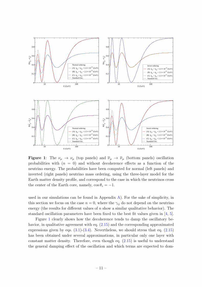
10 100E (GeV)
0
0.2
0.4
0.6
0.8
1
P(ν µ→
ν µ)
Normal ordering
(A) γ31
= γ32
= 2.3 × 10⁻²³
(GeV)
(B) γ21
= γ31
= 2.3 × 10⁻²³
(GeV)
(C) γ21
= γ32
= 2.3 × 10⁻²³
(GeV)
Standard Osc.
10 100E (GeV)
0
0.2
0.4
0.6
0.8
1
P(ν µ→
ν µ)
Normal ordering
(A) γ31
= γ32
= 2.3 × 10⁻²³
(GeV)
(B) γ21
= γ31
= 2.3 × 10⁻²³
(GeV)
(C) γ21
= γ32
= 2.3 × 10⁻²³
(GeV)
Standard Osc.
10 100E (GeV)
0
0.2
0.4
0.6
0.8
1
P(ν µ→
ν µ)
Invert ordering
(A) γ31
= γ32
= 2.3 × 10⁻²³
(GeV)
(B) γ21
= γ31
= 2.3 × 10⁻²³
(GeV)
(C) γ21
= γ32
= 2.3 × 10⁻²³
(GeV)
Standard Osc.
10 100E (GeV)
0
0.2
0.4
0.6
0.8
1
P(ν µ→
ν µ)
Invert ordering
(A) γ31
= γ32
= 2.3 × 10⁻²³
(GeV)
(B) γ21
= γ31
= 2.3 × 10⁻²³
(GeV)
(C) γ21
= γ32
= 2.3 × 10⁻²³
(GeV)
Standard Osc.
Figure 1: The νµ → νµ (top panels) and νµ → νµ (bottom panels) oscillation
probabilities with (n = 0) and without decoherence effects as a function of the
neutrino energy. The probabilities have been computed for normal (left panels) and
inverted (right panels) neutrino mass ordering, using the three-layer model for the
Earth matter density profile, and correspond to the case in which the neutrinos cross
the center of the Earth core, namely, cos θz = −1.
used in our simulations can be found in Appendix A). For the sake of simplicity, in
this section we focus on the case n = 0, where the γij do not depend on the neutrino
energy (the results for different values of n show a similar qualitative behavior). The
standard oscillation parameters have been fixed to the best fit values given in [4, 5].
Figure 1 clearly shows how the decoherence tends to damp the oscillatory be-
havior, in qualitative agreement with eq. (2.15) and the corresponding approximated
expressions given by eqs. (3.1)-(3.4). Nevertheless, we should stress that eq. (2.15)
has been obtained under several approximations, in particular only one layer with
constant matter density. Therefore, even though eq. (2.15) is useful to understand
the general damping effect of the oscillation and which terms are expected to dom-
– 11 –
inate the sensitivity, it may not explain all the features observed in the DeepCore
and IceCube analysis presented in section 5, which has been performed numerically
using the exact probability considering three layers (see appendix A for details).
Since the three γij are not completely independent from one another (see eq. (2.7)),
in view of equations (3.1)-(3.4) and in order to simplify the analysis, hereafter we
will distinguish three different representative cases, where the decoherence effects are
dominated by just one parameter:
(A) Atmospheric limit: γ21 = 0 (γ32 = γ31),
(B) Solar limit I: γ32 = 0 (γ21 = γ31),
(C) Solar limit II: γ31 = 0 (γ21 = γ32).
In appendix B, we will show that the bounds derived in these limits correspond
to the most conservative bounds that can be extracted in the general case. As a
reference value for the decoherence parameters in this section, we have considered
γ = 2.3 · 10−23 GeV, for each of the three limiting cases listed above.
The results in figure 1 show that, for neutrinos with a NO (top left panel),
the impact of decoherence is essentially controlled by γ21, in good agreement with
eq. (3.1): no significant effects are seen in the atmospheric limit (A), while a similar
impact is obtained in the solar limits I (B) and II (C). Conversely, for IO (top right
panel) the effects are dominated by γ31 instead: no effect is observed for the solar
limit II (C), while in scenarios (A) and (B) the effect is very similar. This can
be qualitatively understood from the approximate probability derived in eq. (3.3),
which only depend on the decoherence parameter γ31. On the other hand, in the
antineutrino case for NO (bottom left panel) no observable decoherence effects take
place in case (B), while cases (A) and (C) show a similar behavior, in agreement with
eq. (3.2). Conversely, for IO (bottom right panel) decoherence effects are essentially
controlled by γ21 as shown in eq. (3.4): therefore, no significant effects are observed
in case (A) while a similar impact is obtained for case (B) and (C).
Moreover, it should be pointed out that the transformations listed in Eqs. (3.5)-
(3.7) automatically imply the following equivalence for the results obtained in the
three limiting cases listed above:
(A)NO ←→ (C)IO,
(B)NO ←→ (A)IO, (3.8)
(C)NO ←→ (B)IO.
This is confirmed at the numerical level as it can be easily seen by comparing the
different lines shown in the left (NO) and right (IO) panels in figure 1 for the three
limiting cases.
– 12 –
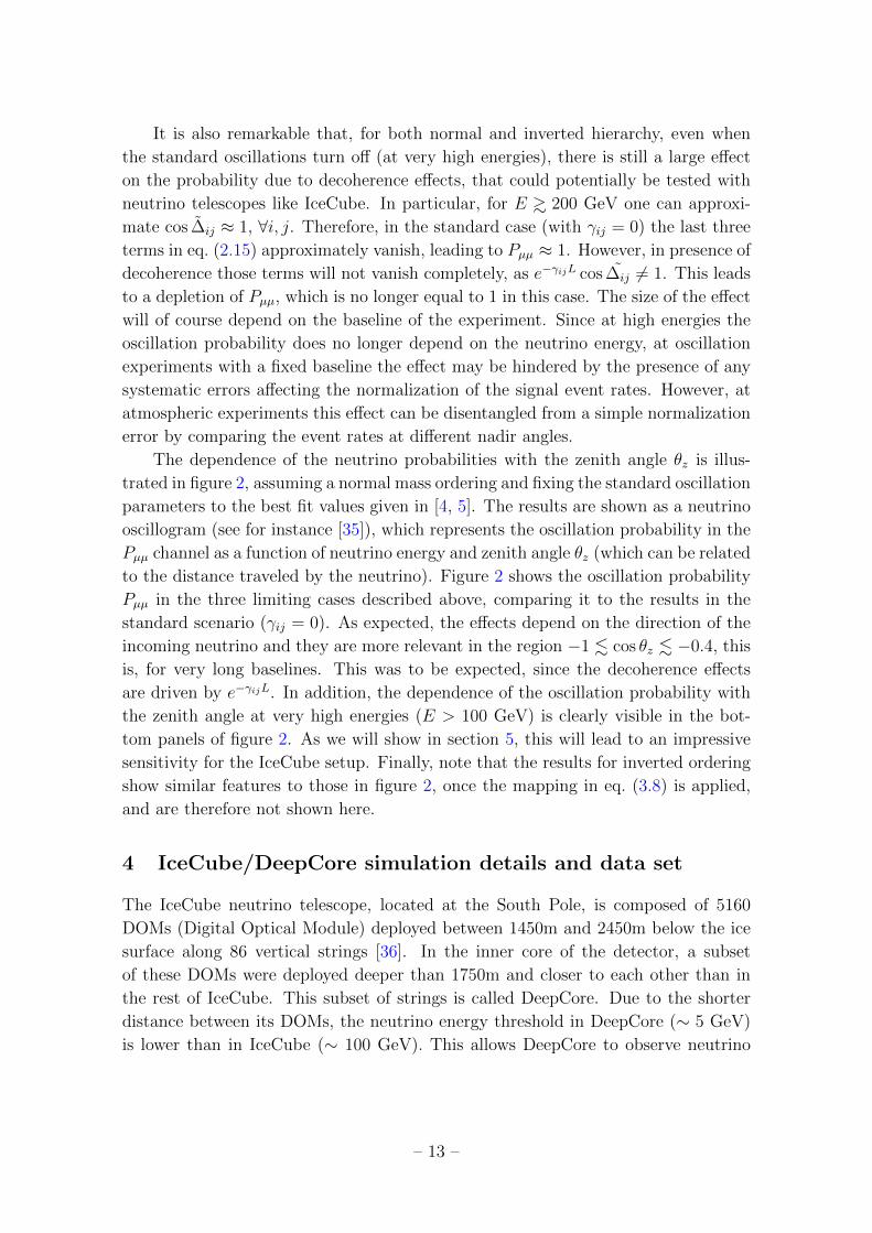
It is also remarkable that, for both normal and inverted hierarchy, even when
the standard oscillations turn off (at very high energies), there is still a large effect
on the probability due to decoherence effects, that could potentially be tested with
neutrino telescopes like IceCube. In particular, for E >∼ 200 GeV one can approxi-
mate cos ∆ij ≈ 1, ∀i, j. Therefore, in the standard case (with γij = 0) the last three
terms in eq. (2.15) approximately vanish, leading to Pµµ ≈ 1. However, in presence of
decoherence those terms will not vanish completely, as e−γijL cos ∆ij 6= 1. This leads
to a depletion of Pµµ, which is no longer equal to 1 in this case. The size of the effect
will of course depend on the baseline of the experiment. Since at high energies the
oscillation probability does no longer depend on the neutrino energy, at oscillation
experiments with a fixed baseline the effect may be hindered by the presence of any
systematic errors affecting the normalization of the signal event rates. However, at
atmospheric experiments this effect can be disentangled from a simple normalization
error by comparing the event rates at different nadir angles.
The dependence of the neutrino probabilities with the zenith angle θz is illus-
trated in figure 2, assuming a normal mass ordering and fixing the standard oscillation
parameters to the best fit values given in [4, 5]. The results are shown as a neutrino
oscillogram (see for instance [35]), which represents the oscillation probability in the
Pµµ channel as a function of neutrino energy and zenith angle θz (which can be related
to the distance traveled by the neutrino). Figure 2 shows the oscillation probability
Pµµ in the three limiting cases described above, comparing it to the results in the
standard scenario (γij = 0). As expected, the effects depend on the direction of the
incoming neutrino and they are more relevant in the region −1 . cos θz . −0.4, this
is, for very long baselines. This was to be expected, since the decoherence effects
are driven by e−γijL. In addition, the dependence of the oscillation probability with
the zenith angle at very high energies (E > 100 GeV) is clearly visible in the bot-
tom panels of figure 2. As we will show in section 5, this will lead to an impressive
sensitivity for the IceCube setup. Finally, note that the results for inverted ordering
show similar features to those in figure 2, once the mapping in eq. (3.8) is applied,
and are therefore not shown here.
4 IceCube/DeepCore simulation details and data set
The IceCube neutrino telescope, located at the South Pole, is composed of 5160
DOMs (Digital Optical Module) deployed between 1450m and 2450m below the ice
surface along 86 vertical strings [36]. In the inner core of the detector, a subset
of these DOMs were deployed deeper than 1750m and closer to each other than in
the rest of IceCube. This subset of strings is called DeepCore. Due to the shorter
distance between its DOMs, the neutrino energy threshold in DeepCore (∼ 5 GeV)
is lower than in IceCube (∼ 100 GeV). This allows DeepCore to observe neutrino
– 13 –
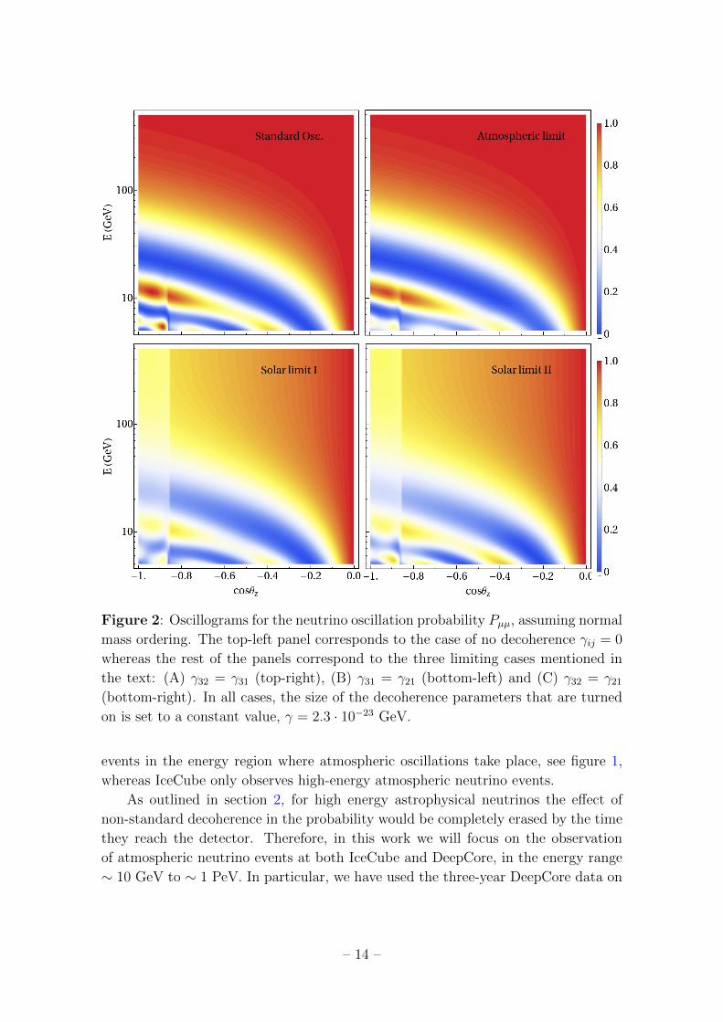
Figure 2: Oscillograms for the neutrino oscillation probability Pµµ, assuming normal
mass ordering. The top-left panel corresponds to the case of no decoherence γij = 0
whereas the rest of the panels correspond to the three limiting cases mentioned in
the text: (A) γ32 = γ31 (top-right), (B) γ31 = γ21 (bottom-left) and (C) γ32 = γ21
(bottom-right). In all cases, the size of the decoherence parameters that are turned
on is set to a constant value, γ = 2.3 · 10−23 GeV.
events in the energy region where atmospheric oscillations take place, see figure 1,
whereas IceCube only observes high-energy atmospheric neutrino events.
As outlined in section 2, for high energy astrophysical neutrinos the effect of
non-standard decoherence in the probability would be completely erased by the time
they reach the detector. Therefore, in this work we will focus on the observation
of atmospheric neutrino events at both IceCube and DeepCore, in the energy range
∼ 10 GeV to ∼ 1 PeV. In particular, we have used the three-year DeepCore data on
– 14 –
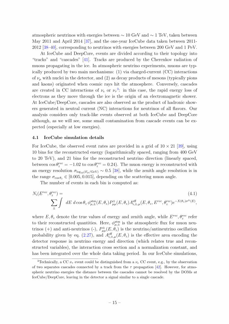
atmospheric neutrinos with energies between ∼ 10 GeV and ∼ 1 TeV, taken between
May 2011 and April 2014 [37], and the one-year IceCube data taken between 2011-
2012 [38–40], corresponding to neutrinos with energies between 200 GeV and 1 PeV.
At IceCube and DeepCore, events are divided according to their topology into
“tracks” and “cascades” [41]. Tracks are produced by the Cherenkov radiation of
muons propagating in the ice. In atmospheric neutrino experiments, muons are typ-
ically produced by two main mechanisms: (1) via charged-current (CC) interactions
of νµ with nuclei in the detector, and (2) as decay products of mesons (typically pions
and kaons) originated when cosmic rays hit the atmosphere. Conversely, cascades
are created in CC interactions of νe or ντ3: in this case, the rapid energy loss of
electrons as they move through the ice is the origin of an electromagnetic shower.
At IceCube/DeepCore, cascades are also observed as the product of hadronic show-
ers generated in neutral current (NC) interactions for neutrinos of all flavors. Our
analysis considers only track-like events observed at both IceCube and DeepCore
although, as we will see, some small contamination from cascade events can be ex-
pected (especially at low energies).
4.1 IceCube simulation details
For IceCube, the observed event rates are provided in a grid of 10 × 21 [39], using
10 bins for the reconstructed energy (logarithmically spaced, ranging from 400 GeV
to 20 TeV), and 21 bins for the reconstructed neutrino direction (linearly spaced,
between cos θrecz = −1.02 to cos θrecz = 0.24). The muon energy is reconstructed with
an energy resolution σlog10(Eµ/GeV) ∼ 0.5 [38], while the zenith angle resolution is in
the range σcos θz ∈ [0.005, 0.015], depending on the scattering muon angle.
The number of events in each bin is computed as:
Ni(Erec, θrecz ) = (4.1)
∑
±
∫dE d cos θz φ
atmµ,±(E, θz)P
±µµ(E, θz)A
effi,±,µ(E, θz, E
rec, θrecz )e−X(θz)σ±(E),
where E, θz denote the true values of energy and zenith angle, while Erec, θrecz refer
to their reconstructed quantities. Here, φatmµ,± is the atmospheric flux for muon neu-
trinos (+) and anti-neutrinos (-), P±µµ(E, θz) is the neutrino/antineutrino oscillation
probability given by eq. (2.27), and Aeffi,±,µ(E, θz) is the effective area encoding the
detector response in neutrino energy and direction (which relates true and recon-
structed variables), the interaction cross section and a normalization constant, and
has been integrated over the whole data taking period. In our IceCube simulations,
3Technically, a CC ντ event could be distinguished from a νe CC event, e.g., by the observation
of two separates cascades connected by a track from the τ propagation [42]. However, for atmo-
spheric neutrino energies the distance between the cascades cannot be resolved by the DOMs at
IceCube/DeepCore, leaving in the detector a signal similar to a single cascade.
– 15 –
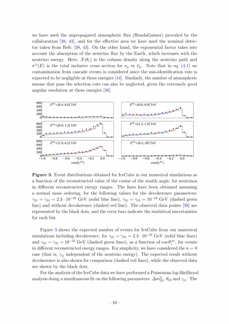
we have used the unpropagated atmospheric flux (HondaGaisser) provided by the
collaboration [38, 43], and for the effective area we have used the nominal detec-
tor taken from Refs. [38, 43]. On the other hand, the exponential factor takes into
account the absorption of the neutrino flux by the Earth, which increases with the
neutrino energy. Here, X(θz) is the column density along the neutrino path and
σ±(E) is the total inclusive cross section for νµ or νµ. Note that in eq. (4.1) no
contamination from cascade events is considered since the mis-identification rate is
expected to be negligible at these energies [44]. Similarly, the number of atmospheric
muons that pass the selection cuts can also be neglected, given the extremely good
angular resolution at these energies [38].
0
200
400
600
800E
rec=[0.4, 0.6] TeV Erec=[0.6, 0.9] TeV
0200400600800
Erec=[0.9, 1.3] TeV
Erec=[1.3, 1.9] TeV
-1.0 -0.8 -0.6 -0.4 -0.2 0.00
200
400
600
800
cos(θzrec)
Erec=[1.9, 6.2] TeV
-1.0 -0.8 -0.6 -0.4 -0.2 0.0
cos(θzrec)
Erec=[6.2, 20] TeV
Figure 3: Event distributions obtained for IceCube in our numerical simulations as
a function of the reconstructed value of the cosine of the zenith angle, for neutrinos
in different reconstructed energy ranges. The lines have been obtained assuming
a normal mass ordering, for the following values for the decoherence parameters:
γ21 = γ31 = 2.3 · 10−23 GeV (solid blue line), γ21 = γ31 = 10−22 GeV (dashed green
line) and without decoherence (dashed red line). The observed data points [39] are
represented by the black dots, and the error bars indicate the statistical uncertainties
for each bin.
Figure 3 shows the expected number of events for IceCube from our numerical
simulations including decoherence, for γ21 = γ31 = 2.3 · 10−23 GeV (solid blue lines)
and γ21 = γ31 = 10−22 GeV (dashed green lines), as a function of cos θrecz , for events
in different reconstructed energy ranges. For simplicity, we have considered the n = 0
case (that is, γij independent of the neutrino energy). The expected result without
decoherence is also shown for comparison (dashed red lines), while the observed data
are shown by the black dots.
For the analysis of the IceCube data we have performed a Poissonian log-likelihood
analysis doing a simultaneous fit on the following parameters: ∆m232, θ23 and γij. The
– 16 –
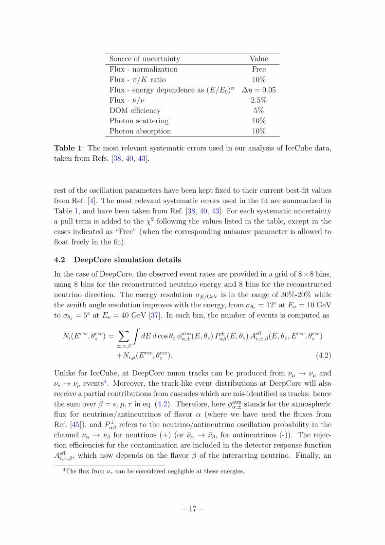
Source of uncertainty Value
Flux - normalization Free
Flux - π/K ratio 10%
Flux - energy dependence as (E/E0)η ∆η = 0.05
Flux - ν/ν 2.5%
DOM efficiency 5%
Photon scattering 10%
Photon absorption 10%
Table 1: The most relevant systematic errors used in our analysis of IceCube data,
taken from Refs. [38, 40, 43].
rest of the oscillation parameters have been kept fixed to their current best-fit values
from Ref. [4]. The most relevant systematic errors used in the fit are summarized in
Table 1, and have been taken from Ref. [38, 40, 43]. For each systematic uncertainty
a pull term is added to the χ2 following the values listed in the table, except in the
cases indicated as “Free” (when the corresponding nuisance parameter is allowed to
float freely in the fit).
4.2 DeepCore simulation details
In the case of DeepCore, the observed event rates are provided in a grid of 8×8 bins,
using 8 bins for the reconstructed neutrino energy and 8 bins for the reconstructed
neutrino direction. The energy resolution σE/GeV is in the range of 30%-20% while
the zenith angle resolution improves with the energy, from σθz = 12◦ at Eν = 10 GeV
to σθz = 5◦ at Eν = 40 GeV [37]. In each bin, the number of events is computed as
Ni(Erec, θrecz ) =
∑
±,α,β
∫dE d cos θz φ
atmα,±(E, θz)P
±αβ(E, θz)A
effi,±,β(E, θz, E
rec, θrecz )
+Ni,µ(Erec, θrecz ). (4.2)
Unlike for IceCube, at DeepCore muon tracks can be produced from νµ → νµ and
νe → νµ events4. Moreover, the track-like event distributions at DeepCore will also
receive a partial contributions from cascades which are mis-identified as tracks: hence
the sum over β = e, µ, τ in eq. (4.2). Therefore, here φatmα,± stands for the atmospheric
flux for neutrinos/antineutrinos of flavor α (where we have used the fluxes from
Ref. [45]), and P±αβ refers to the neutrino/antineutrino oscillation probability in the
channel να → νβ for neutrinos (+) (or να → νβ, for antineutrinos (-)). The rejec-
tion efficiencies for the contamination are included in the detector response function
Aeffi,±,β, which now depends on the flavor β of the interacting neutrino. Finally, an
4The flux from ντ can be considered negligible at these energies.
– 17 –

estimate of the atmospheric muons that overcome the selection criteria (taken from
Ref. [37, 43]) is also added for each bin in reconstructed variables, Ni,µ.
Figure 4 shows the expected number of events for DeepCore obtained from our
numerical simulations including decoherence, for γ21 = γ31 = 2.3 · 10−23 GeV (solid
blue lines) and γ21 = γ31 = 10−22 GeV (dashed green lines), as a function of cos θrecz ,
for events in different reconstructed energy ranges. For simplicity, we have considered
the n = 0 case (that is, γij independent of the neutrino energy). The expected
result without decoherence is also shown for comparison (dashed red lines), while
the observed data are shown by the black dots.
0
50
100
150
200E
rec=[6, 8] GeV Erec=[8, 10] GeV
0
50
100
150
200E
rec=[10, 14] GeV Erec=[14, 18] GeV
0
50
100
150
200E
rec=[24, 32] GeV Erec=[24, 32] GeV
-1.0 -0.8 -0.6 -0.4 -0.2 0.00
50
100
150
200
cos(θzrec)
Erec=[32, 42] GeV
-1.0 -0.8 -0.6 -0.4 -0.2 0.0
cos(θzrec)
Erec=[42, 56] GeV
Figure 4: Event distributions obtained for DeepCore in our numerical simulations as
a function of the reconstructed values of the cosine of the zenith angle, for neutrinos
in different reconstructed energy ranges. The lines have been obtained assuming
a normal mass ordering, for the following values for the decoherence parameters:
γ21 = γ31 = 2.3 · 10−23 GeV (solid blue line), γ21 = γ31 = 10−22 GeV (dashed green
line) and without decoherence (dashed red line). The observed data points [37] are
represented by the black dots, and the error bars indicate the statistical uncertainties
for each bin.
In this work a Gaussian maximum likelihood is used to analyze the DeepCore
data, performing a simultaneous fit on the following parameters: ∆m232, θ23 and γij.
The rest of the oscillation parameters have been kept fixed to their current best-fit
values from Ref. [4]. The systematics used in the fit are those associated with the
flux, the detector response and the atmospheric muons given in Ref. [37] and are
summarized in Table 2. For each systematic uncertainty a pull term is added to the
χ2 following the values listed in the table, except in the cases indicated as “Free”
(when the corresponding nuisance parameter is allowed to float freely in the fit). We
– 18 –
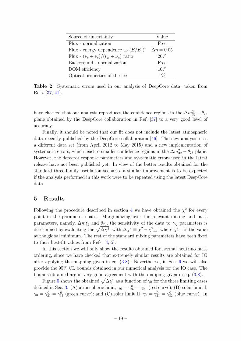
Source of uncertainty Value
Flux - normalization Free
Flux - energy dependence as (E/E0)η ∆η = 0.05
Flux - (νe + νe)/(νµ + νµ) ratio 20%
Background - normalization Free
DOM efficiency 10%
Optical properties of the ice 1%
Table 2: Systematic errors used in our analysis of DeepCore data, taken from
Refs. [37, 41].
have checked that our analysis reproduces the confidence regions in the ∆m232 − θ23
plane obtained by the DeepCore collaboration in Ref. [37] to a very good level of
accuracy.
Finally, it should be noted that our fit does not include the latest atmospheric
data recently published by the DeepCore collaboration [46]. The new analysis uses
a different data set (from April 2012 to May 2015) and a new implementation of
systematic errors, which lead to smaller confidence regions in the ∆m232 − θ23 plane.
However, the detector response parameters and systematic errors used in the latest
release have not been published yet. In view of the better results obtained for the
standard three-family oscillation scenario, a similar improvement is to be expected
if the analysis performed in this work were to be repeated using the latest DeepCore
data.
5 Results
Following the procedure described in section 4 we have obtained the χ2 for every
point in the parameter space. Marginalizing over the relevant mixing and mass
parameters, namely, ∆m232 and θ23, the sensitivity of the data to γij parameters is
determined by evaluating the√
∆χ2, with ∆χ2 ≡ χ2−χ2min, where χ2
min is the value
at the global minimum. The rest of the standard mixing parameters have been fixed
to their best-fit values from Refs. [4, 5].
In this section we will only show the results obtained for normal neutrino mass
ordering, since we have checked that extremely similar results are obtained for IO
after applying the mapping given in eq. (3.8). Nevertheless, in Sec. 6 we will also
provide the 95% CL bounds obtained in our numerical analysis for the IO case. The
bounds obtained are in very good agreement with the mapping given in eq. (3.8).
Figure 5 shows the obtained√
∆χ2 as a function of γ0 for the three limiting cases
defined in Sec. 3: (A) atmospheric limit, γ0 = γ032 = γ0
31 (red curve); (B) solar limit I,
γ0 = γ021 = γ0
31 (green curve); and (C) solar limit II, γ0 = γ021 = γ0
32 (blue curve). In
– 19 –
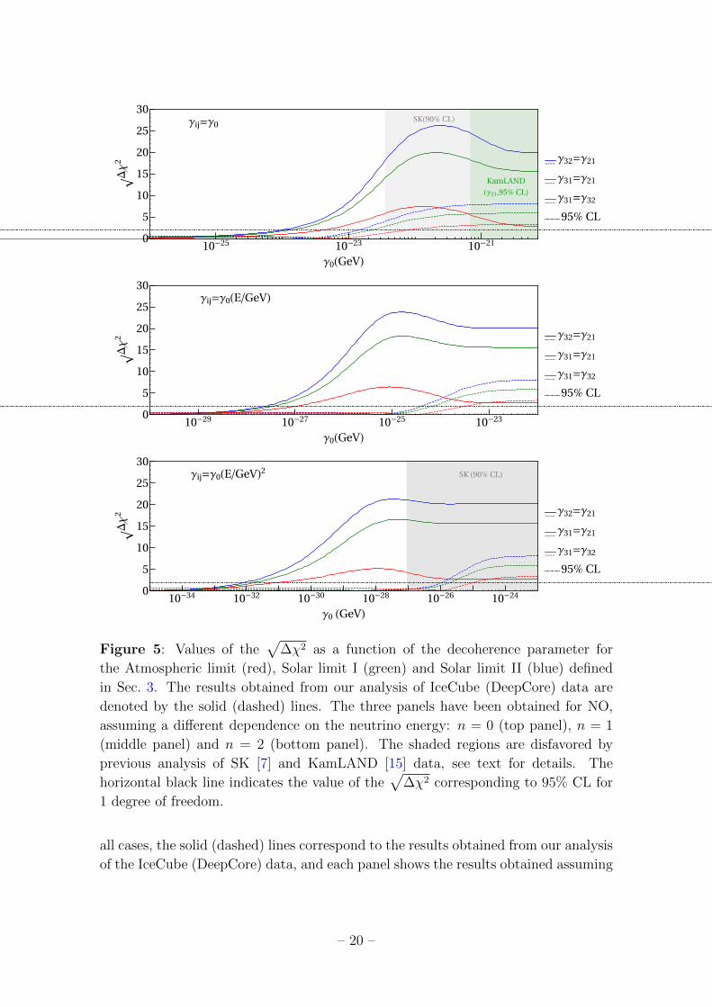
10-25 10-23 10-210
5
10
15
20
25
30
γ0(GeV)
√Δχ
2SK(90% CL)
KamLAND
(γ21,95% CL)
γij=γ0
-----
γ32=γ21
-----
γ31=γ21
-----
γ31=γ32
95% CL
10-29 10-27 10-25 10-230
5
10
15
20
25
30
γ0(GeV)
√Δχ
2
γij=γ0(E/GeV)
-----
γ32=γ21
-----
γ31=γ21
-----
γ31=γ32
95% CL
10-34 10-32 10-30 10-28 10-26 10-240
5
10
15
20
25
30
γ0 (GeV)
√Δχ
2
SK (90% CL)γij=γ0(E/GeV)2
-----
γ32=γ21
-----
γ31=γ21
-----
γ31=γ32
95% CL
Figure 5: Values of the√
∆χ2 as a function of the decoherence parameter for
the Atmospheric limit (red), Solar limit I (green) and Solar limit II (blue) defined
in Sec. 3. The results obtained from our analysis of IceCube (DeepCore) data are
denoted by the solid (dashed) lines. The three panels have been obtained for NO,
assuming a different dependence on the neutrino energy: n = 0 (top panel), n = 1
(middle panel) and n = 2 (bottom panel). The shaded regions are disfavored by
previous analysis of SK [7] and KamLAND [15] data, see text for details. The
horizontal black line indicates the value of the√
∆χ2 corresponding to 95% CL for
1 degree of freedom.
all cases, the solid (dashed) lines correspond to the results obtained from our analysis
of the IceCube (DeepCore) data, and each panel shows the results obtained assuming
– 20 –
a different energy dependence for the decoherence parameters, see eq. (2.13): n = 0
(top panel), n = 1 (middle panel) and n = 2 (bottom panel). The shaded regions are
disfavored by previous analysis of SK [7] (90% CL) and KamLAND [15] data (95%
CL). As explained in section 3, the KamLAND constraints derived in [15] apply to
γ012 (solar limits) while it is not clear to which γij the bounds from SK obtained in [7]
would apply, since this depends on the true neutrino mass ordering (which is yet
unknown).
Figure 5 shows that for both DeepCore and IceCube the best sensitivity is
achieved for the solar limits (B) and (C) while the weakest limit is obtained in
the atmospheric limit (A). In particular, the strongest bound is obtained for (C).
This is in agreement with the behaviour of the oscillation probability in presence of
strong matter effects, discussed in section 3. On one hand, as shown in section 3,
for NO the decoherence effects are mainly driven by γ21 in the neutrino channel and
γ32 in the antineutrino channel. On the other hand, the number of antineutrino
events is going to be suppressed with respect to the neutrino case, due to the smaller
cross section and flux. Hence, the best sensitivity is expected for case (C), where
γ0 = γ021 = γ0
32, since both neutrinos and antineutrinos are sensitive to decoherence
effects. Conversely, in case (B), where γ0 = γ021 = γ0
31, only neutrinos are sensitive to
decoherence effects, and therefore some sensitivity is lost with respect to the results
for case (C). Finally, in case (A), with γ0 = γ032 = γ0
31, the bounds come mainly
from the impact of decoherence on the antineutrino event rates and, since these are
much smaller than in the neutrino case, the obtained bounds are much weaker when
compared to the results obtained in case (B).
Figure 5 shows a flat asymptotic feature of the√
∆χ2 for large values of γ0, where
the sensitivity becomes independent of γ0. In fact, for IceCube there is a decrease
in sensitivity for values of γ above a certain range: for example, for n = 0 the best
sensitivity is achieved for γ0 ∼ O(10−22) GeV while it decreases for higher values.
This behaviour can be understood as follows. For the neutrino energies observed at
IceCube (above 100 GeV) the oscillation phases do not develope and the probabilities
do not depend on the energy (cos ∆ij ≈ 1 in eq. (2.15)). Therefore, at IceCube the
sensitivity to the decoherence effects comes from the observation of a non-standard
behaviour of the number of events with the zenith angle. Naively, eq. (2.14) gives
the values of L and γ that yield a large effect. Considering n = 0, for example,
where there is a one-to-one relation between the two, we get that for γ0 ∼ 10−22 GeV
the effect will be maximal for distances of the order L ∼ O(103) km. This is the
typical distance traveled by atmospheric neutrinos crossing the Earth and therefore
the sensitivity of IceCube is maximized in this range. Conversely, for larger (smaller)
values of γ0, only neutrinos coming from the most horizontal (vertical) directions are
affected, leading to a reduced impact on the χ2.
From the comparison between the different panels in figure 5 we can see that
the limits change considerably with the value of n, which parametrizes the energy
– 21 –

●
●
●
●
●
●
●
●
●
●
●
●
●
●
●
▲
▲
▲
▲
▲
▲
▲
▲
▲
▲
▲
▲
▲
▲
▲
-2 -1 0 1 2
10-32
10-29
10-26
10-23
10-20
10-17
n
γ0(G
eV)
γ=γ0(E/GeV)n
▲γ31=γ32
▲γ21=γ31
▲γ21=γ32
Figure 6: 95% CL bounds on the decoherence parameters γ0, for NO, as a (discrete)
function of the power-law index n for for the Atmospheric limit (red), Solar limit
I (green) and Solar limit II (blue). The solid circles (triangles) correspond to the
DeepCore (IceCube) analysis.
dependence of the decoherence parameters (see eq. (2.13)). In particular, we observe
in figure 5 that the sensitivity improves as n is increased and that, as the vaule of n is
increased, the results for IceCube improve much faster (compared to DeepCore) due
to the higher neutrino energies considered. The behaviour of the sensitivities with
the value of n is better appreciated in figure 6, where we show the bounds obtained
at 95% CL (for 1 degree of freedom) as a (discrete) function of the power-law index
n, for n = −2,−1, 0, 1 and 2. The DeepCore bounds are represented by solid circles
while the IceCube constraints are given by the solid triangles. The results seem to
follow the linear relation
ln(γ0/GeV) = constant− n ln(E0/GeV), (5.1)
where E0 ' 2.5 TeV (30 GeV) for IceCube (DeepCore). This can be understood
as follows. Decoherence effects enter the oscillation probabilities only through the
factor γL = γ0(E/GeV)nL, for any value of n. Naively, we expect that the sensitivity
limit is obtained for γL ∼ O(1) (although the precise value will eventually depend
on the neutrino mass ordering, on the particular γij which drives the sensitivity,
and on the data set considered). Taking the logarithm of γ0(E/GeV)nL = constant,
we reproduce eq. (5.1). At first approximation, the value of E0 in eq. (5.1) can be
estimated as the average energy of the IceCube and DeepCore event distributions,
– 22 –
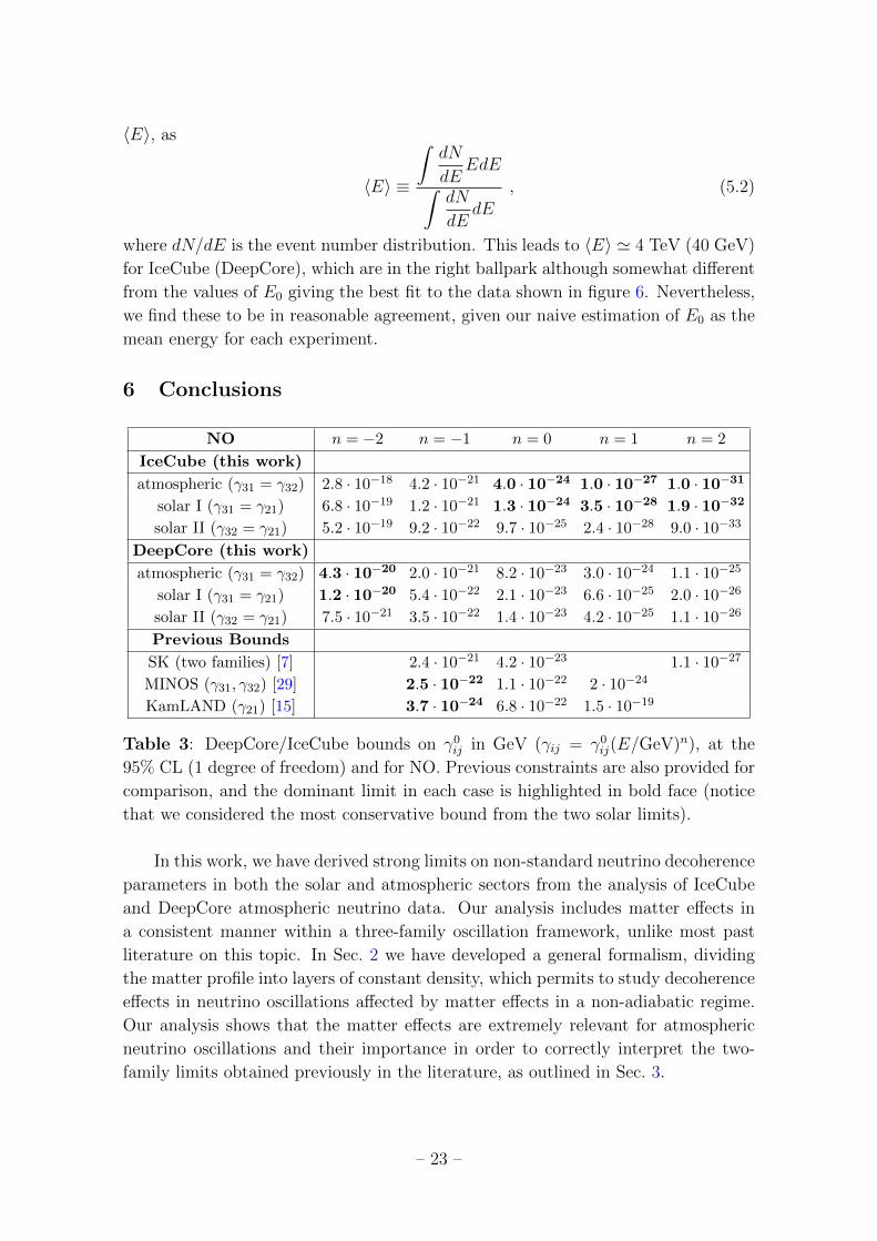
〈E〉, as
〈E〉 ≡
∫dN
dEEdE
∫dN
dEdE
, (5.2)
where dN/dE is the event number distribution. This leads to 〈E〉 ' 4 TeV (40 GeV)
for IceCube (DeepCore), which are in the right ballpark although somewhat different
from the values of E0 giving the best fit to the data shown in figure 6. Nevertheless,
we find these to be in reasonable agreement, given our naive estimation of E0 as the
mean energy for each experiment.
6 Conclusions
NO n = −2 n = −1 n = 0 n = 1 n = 2
IceCube (this work)
atmospheric (γ31 = γ32) 2.8 · 10−18 4.2 · 10−21 4.0 · 10−24 1.0 · 10−27 1.0 · 10−31solar I (γ31 = γ21) 6.8 · 10−19 1.2 · 10−21 1.3 · 10−24 3.5 · 10−28 1.9 · 10−32solar II (γ32 = γ21) 5.2 · 10−19 9.2 · 10−22 9.7 · 10−25 2.4 · 10−28 9.0 · 10−33
DeepCore (this work)
atmospheric (γ31 = γ32) 4.3 · 10−20 2.0 · 10−21 8.2 · 10−23 3.0 · 10−24 1.1 · 10−25
solar I (γ31 = γ21) 1.2 · 10−20 5.4 · 10−22 2.1 · 10−23 6.6 · 10−25 2.0 · 10−26
solar II (γ32 = γ21) 7.5 · 10−21 3.5 · 10−22 1.4 · 10−23 4.2 · 10−25 1.1 · 10−26
Previous Bounds
SK (two families) [7] 2.4 · 10−21 4.2 · 10−23 1.1 · 10−27
MINOS (γ31, γ32) [29] 2.5 · 10−22 1.1 · 10−22 2 · 10−24
KamLAND (γ21) [15] 3.7 · 10−24 6.8 · 10−22 1.5 · 10−19
Table 3: DeepCore/IceCube bounds on γ0ij in GeV (γij = γ0
ij(E/GeV)n), at the
95% CL (1 degree of freedom) and for NO. Previous constraints are also provided for
comparison, and the dominant limit in each case is highlighted in bold face (notice
that we considered the most conservative bound from the two solar limits).
In this work, we have derived strong limits on non-standard neutrino decoherence
parameters in both the solar and atmospheric sectors from the analysis of IceCube
and DeepCore atmospheric neutrino data. Our analysis includes matter effects in
a consistent manner within a three-family oscillation framework, unlike most past
literature on this topic. In Sec. 2 we have developed a general formalism, dividing
the matter profile into layers of constant density, which permits to study decoherence
effects in neutrino oscillations affected by matter effects in a non-adiabatic regime.
Our analysis shows that the matter effects are extremely relevant for atmospheric
neutrino oscillations and their importance in order to correctly interpret the two-
family limits obtained previously in the literature, as outlined in Sec. 3.
– 23 –

We have found that the sensitivity to decoherence effects depends strongly on the
neutrino mass ordering and on whether the sensitivity is dominated by the neutrino
or antineutrino event rates. For neutrinos, the decoherence effects at high energies are
mainly driven by γ21 (γ31) for normal (inverted) ordering, while in the antineutrino
case they are essentially controlled by γ32 (γ21) for normal (inverted) ordering. This
means that, considering a three-family framework including matter effects is essential
when decoherence effects in atmospheric neutrino oscillations are studied. Our results
are summarized in table 3 for normal ordering (NO) of neutrino masses, and in table 4
for inverted ordering (IO). The two tables summarize, together with the most relevant
bounds present in the literature, the 95% CL bounds extracted from our analysis
of DeepCore and IceCube atmospheric neutrino data, for the three limiting cases
considered in this work: (A) atmospheric limit (γ21 = 0), (B) solar limit I (γ32 = 0)
and (C) solar limit II (γ31 = 0). In Appendix B we show that the bounds derived in
these limits correspond to the most conservative results that can be extracted in the
general case.
In this work, we considered a general dependence of the decoherence parameters
with the energy, as γij = γ0ij (E/GeV)n with n = ±2, 0,±2. Our results improve over
previous bounds for most of the cases studied, with the exception of the n = −1
case. For n = −1, KamLAND gives the dominant bound on γ21 while MINOS gives
the strongest constraints on γ31 and γ32. Indeed, both KamLAND and MINOS are
also expected to give the strongest bound for n = −2, although to the best of our
knowledge no analysis has been performed for this case yet. Our results show that,
for n = 0 (which is the case most commonly considered in the literature), IceCube
improves the bound on γ31 and γ32 in (more than) one order of magnitude with
respect to the SK constraint, obtained in a simplified two-family approximation, and
by more than one order (almost two orders) of magnitude for NO (IO) with respect to
the KamLAND constraint on γ21. In particular, we find that the reference value for
γ23 considered in Ref. [17] to explain the small tension previously reported between
NOvA and SK data is indeed already excluded by IceCube data. Regarding the
cases with n = 1, 2, we find that the sensitivity of IceCube is particularly strong.
For instance, IceCube improves the bound from KamLAND on γ21 by almost 9 (8)
orders of magnitude for n = 1 and NO (IO), while for n = 2 the bound on γ31 and
γ32 is improved in 4 (5) orders of magnitude with respect to the SK limit for NO
(IO).
Acknowledgments
We thank C. Gonzalez-Garcıa, M. Maltoni and J. Salvado for useful discussions. JLP,
IMS and HN thank the hospitality of the Fermilab Theoretical Physics Department
where this work was initiated. HN also thanks the hospitality of the CERN Theoreti-
cal Physics Department where the final part of this work was done. HN was supported
– 24 –
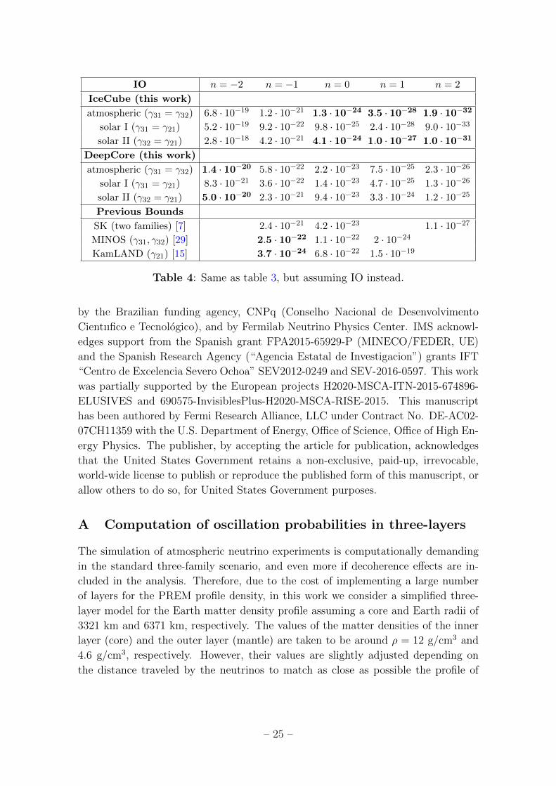
IO n = −2 n = −1 n = 0 n = 1 n = 2
IceCube (this work)
atmospheric (γ31 = γ32) 6.8 · 10−19 1.2 · 10−21 1.3 · 10−24 3.5 · 10−28 1.9 · 10−32solar I (γ31 = γ21) 5.2 · 10−19 9.2 · 10−22 9.8 · 10−25 2.4 · 10−28 9.0 · 10−33
solar II (γ32 = γ21) 2.8 · 10−18 4.2 · 10−21 4.1 · 10−24 1.0 · 10−27 1.0 · 10−31DeepCore (this work)
atmospheric (γ31 = γ32) 1.4 · 10−20 5.8 · 10−22 2.2 · 10−23 7.5 · 10−25 2.3 · 10−26
solar I (γ31 = γ21) 8.3 · 10−21 3.6 · 10−22 1.4 · 10−23 4.7 · 10−25 1.3 · 10−26
solar II (γ32 = γ21) 5.0 · 10−20 2.3 · 10−21 9.4 · 10−23 3.3 · 10−24 1.2 · 10−25
Previous Bounds
SK (two families) [7] 2.4 · 10−21 4.2 · 10−23 1.1 · 10−27
MINOS (γ31, γ32) [29] 2.5 · 10−22 1.1 · 10−22 2 · 10−24
KamLAND (γ21) [15] 3.7 · 10−24 6.8 · 10−22 1.5 · 10−19
Table 4: Same as table 3, but assuming IO instead.
by the Brazilian funding agency, CNPq (Conselho Nacional de Desenvolvimento
Cientııfico e Tecnologico), and by Fermilab Neutrino Physics Center. IMS acknowl-
edges support from the Spanish grant FPA2015-65929-P (MINECO/FEDER, UE)
and the Spanish Research Agency (“Agencia Estatal de Investigacion”) grants IFT
“Centro de Excelencia Severo Ochoa” SEV2012-0249 and SEV-2016-0597. This work
was partially supported by the European projects H2020-MSCA-ITN-2015-674896-
ELUSIVES and 690575-InvisiblesPlus-H2020-MSCA-RISE-2015. This manuscript
has been authored by Fermi Research Alliance, LLC under Contract No. DE-AC02-
07CH11359 with the U.S. Department of Energy, Office of Science, Office of High En-
ergy Physics. The publisher, by accepting the article for publication, acknowledges
that the United States Government retains a non-exclusive, paid-up, irrevocable,
world-wide license to publish or reproduce the published form of this manuscript, or
allow others to do so, for United States Government purposes.
A Computation of oscillation probabilities in three-layers
The simulation of atmospheric neutrino experiments is computationally demanding
in the standard three-family scenario, and even more if decoherence effects are in-
cluded in the analysis. Therefore, due to the cost of implementing a large number
of layers for the PREM profile density, in this work we consider a simplified three-
layer model for the Earth matter density profile assuming a core and Earth radii of
3321 km and 6371 km, respectively. The values of the matter densities of the inner
layer (core) and the outer layer (mantle) are taken to be around ρ = 12 g/cm3 and
4.6 g/cm3, respectively. However, their values are slightly adjusted depending on
the distance traveled by the neutrinos to match as close as possible the profile of
– 25 –
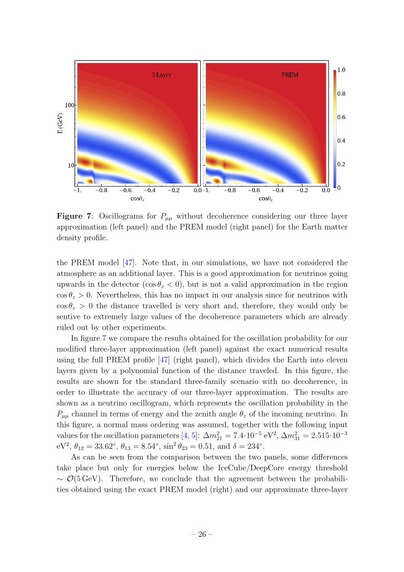
Figure 7: Oscillograms for Pµµ without decoherence considering our three layer
approximation (left panel) and the PREM model (right panel) for the Earth matter
density profile.
the PREM model [47]. Note that, in our simulations, we have not considered the
atmosphere as an additional layer. This is a good approximation for neutrinos going
upwards in the detector (cos θz < 0), but is not a valid approximation in the region
cos θz > 0. Nevertheless, this has no impact in our analysis since for neutrinos with
cos θz > 0 the distance travelled is very short and, therefore, they would only be
sentive to extremely large values of the decoherence parameters which are already
ruled out by other experiments.
In figure 7 we compare the results obtained for the oscillation probability for our
modified three-layer approximation (left panel) against the exact numerical results
using the full PREM profile [47] (right panel), which divides the Earth into eleven
layers given by a polynomial function of the distance traveled. In this figure, the
results are shown for the standard three-family scenario with no decoherence, in
order to illustrate the accuracy of our three-layer approximation. The results are
shown as a neutrino oscillogram, which represents the oscillation probability in the
Pµµ channel in terms of energy and the zenith angle θz of the incoming neutrino. In
this figure, a normal mass ordering was assumed, together with the following input
values for the oscillation parameters [4, 5]: ∆m221 = 7.4·10−5 eV2, ∆m2
31 = 2.515·10−3
eV2, θ12 = 33.62◦, θ13 = 8.54◦, sin2 θ23 = 0.51, and δ = 234◦.
As can be seen from the comparison between the two panels, some differences
take place but only for energies below the IceCube/DeepCore energy threshold
∼ O(5 GeV). Therefore, we conclude that the agreement between the probabili-
ties obtained using the exact PREM model (right) and our approximate three-layer
– 26 –
model (left) is sufficiently good for the purposes of this work. We have also checked
that, using our simplified three-layer model applied to the standard case without de-
coherence, we are able to reproduce up to a very good approximation the DeepCore
oscillation fit for the atmospheric parameters θ23 and ∆m232 [37].
B Five-dimensional analysis
The γij are not completely independent parameters as we have already pointed out
(see eq. (2.7)). In order to simplify the analysis, in this work we have studied three
different representative cases: (A) Atmospheric limit, γ21 = 0 (γ32 = γ31); (B) Solar
limit I, γ32 = 0 (γ21 = γ31); and (C) Solar limit II, γ31 = 0 (γ21 = γ32). Considering
these one-γij dominated cases is expected to be a very good approximation in view
of equations (3.1)-(3.4). In any case, in this Appendix we will show that the results
obtained in these simplified scenarios apply to the more general case in which the
three γij are different from zero.
Let us assume that just one Dm matrix contributes to the decoherence term of
the evolution equations given by eq. (2.2). In such a case, one of the γij parameters
is a function of the other two γij. Without loss of generality, we chose γ21 and γ31 as
the free parameters and γ32 is then given by
γ32 = (√γ21 ±
√γ31)2 . (B.1)
In order to understand how general are the results presented in sec. 5, we have
performed a five-dimensional analysis varying γ21, γ31, θ23 and ∆m232 in the fit, and
imposing the constraint given by the equation above. In figure 8 we show the√
∆χ2
obtained from the five-dimensional DeepCore analysis as a function of γ21 (dashed
green curve) and γ31 (dashed red curve), marginalizing over the rest of the free
parameters, for the n = 0 case (the same conclusions apply to the other cases studied
in this work). For the sake of comparison, the√
∆χ2 associated to the atmospheric
(solid red curve), solar I (solid green curve) and solar II (solid blue curve) limits
is also included in the same figure. NO was assumed but the results can be easily
extrapolated to the IO case using the mapping given in eq. (3.8).
Figure 8 shows that the five-dimensional√
∆χ2 distribution projected into γ31
coincides with the Atmospheric limit one, while when it is projected into γ21 resembles
the most conservative of the two solar limits. This is due to the marginalization over
the parameters which are not shown. For instance, in the case of γ21 the marginaliza-
tion selects, between the two solar limits, the most conservative result. We conclude
therefore that our analysis distinguishing the three limits (A), (B) and (C), provides
the most conservative bounds that can be applied to the general case in which the
three γij are different from zero.
– 27 –

10-25 10-24 10-23 10-22 10-210
2
4
6
8
10
γ0(GeV)
√Δχ
2SK(90% CL)
KamLAND
(γ21,95% CL)
γij=γ0
γ32=γ21
γ31=γ21
γ31=γ32
γ21
γ31
95% CL
Figure 8:√
∆χ2 obtained from the five-dimensional DeepCore analysis as a function
of γ21 (dashed green curve) and γ31 (dashed red curve), marginalizing over the rest
of the free parameters, for the n = 0 case and NO. The√
∆χ2 for the Atmospheric
(solid red curve), Solar I (solid green curve) and Solar II (solid blue curve) limits is
also shown.
References
[1] Daya Bay collaboration, F. P. An et al., New Measurement of Antineutrino
Oscillation with the Full Detector Configuration at Daya Bay, Phys. Rev. Lett. 115
(2015) 111802, [1505.03456].
[2] A. Izmaylov, ““T2K Neutrino Experiment. Recent Results and Plans.” Talk given at
the Flavour Physics Conference, Quy Nhon, Vietnam, August 13–19, 2017.”
http://v17flavour.in2p3.fr/ThursdayAfternoon/Izmaylov.pdf.
[3] Alexander Radovic, ““Results from NOvA”, Fermilab Joint
Experimental-Theoretical Physics Seminar, January 12, 2018..”
http://theory.fnal.gov/events/event/results-from-nova/.
[4] “NuFIT 3.2 (2018).” Results available at: http://www.nu-fit.org.
[5] I. Esteban, M. C. Gonzalez-Garcia, M. Maltoni, I. Martinez-Soler and T. Schwetz,
Updated fit to three neutrino mixing: exploring the accelerator-reactor
complementarity, JHEP 01 (2017) 087, [1611.01514].
[6] F. Benatti and R. Floreanini, Open system approach to neutrino oscillations, JHEP
02 (2000) 032, [hep-ph/0002221].
[7] E. Lisi, A. Marrone and D. Montanino, Probing possible decoherence effects in
atmospheric neutrino oscillations, Phys. Rev. Lett. 85 (2000) 1166–1169,
[hep-ph/0002053].
[8] A. M. Gago, E. M. Santos, W. J. C. Teves and R. Zukanovich Funchal, Quantum
dissipative effects and neutrinos: Current constraints and future perspectives, Phys.
Rev. D63 (2001) 073001, [hep-ph/0009222].
[9] A. M. Gago, E. M. Santos, W. J. C. Teves and R. Zukanovich Funchal, A Study on
– 28 –
quantum decoherence phenomena with three generations of neutrinos,
hep-ph/0208166.
[10] D. Morgan, E. Winstanley, J. Brunner and L. F. Thompson, Probing quantum
decoherence in atmospheric neutrino oscillations with a neutrino telescope,
Astropart. Phys. 25 (2006) 311–327, [astro-ph/0412618].
[11] D. Hooper, D. Morgan and E. Winstanley, Probing quantum decoherence with
high-energy neutrinos, Phys. Lett. B609 (2005) 206–211, [hep-ph/0410094].
[12] G. L. Fogli, E. Lisi, A. Marrone, D. Montanino and A. Palazzo, Probing
non-standard decoherence effects with solar and KamLAND neutrinos, Phys. Rev.
D76 (2007) 033006, [0704.2568].
[13] Y. Farzan, T. Schwetz and A. Y. Smirnov, Reconciling results of LSND, MiniBooNE
and other experiments with soft decoherence, JHEP 07 (2008) 067, [0805.2098].
[14] P. Bakhti, Y. Farzan and T. Schwetz, Revisiting the quantum decoherence scenario
as an explanation for the LSND anomaly, JHEP 05 (2015) 007, [1503.05374].
[15] G. Balieiro Gomes, M. M. Guzzo, P. C. de Holanda and R. L. N. Oliveira,
Parameter Limits for Neutrino Oscillation with Decoherence in KamLAND, Phys.
Rev. D95 (2017) 113005, [1603.04126].
[16] R. L. N. Oliveira, Dissipative Effect in Long Baseline Neutrino Experiments, Eur.
Phys. J. C76 (2016) 417, [1603.08065].
[17] J. A. B. Coelho, W. A. Mann and S. S. Bashar, Nonmaximal θ23 mixing at NOvA
from neutrino decoherence, Phys. Rev. Lett. 118 (2017) 221801, [1702.04738].
[18] J. a. A. B. Coelho and W. A. Mann, Decoherence, matter effect, and neutrino
hierarchy signature in long baseline experiments, Phys. Rev. D96 (2017) 093009,
[1708.05495].
[19] J. A. Carpio, E. Massoni and A. M. Gago, Revisiting quantum decoherence in the
matter neutrino oscillation framework, 1711.03680.
[20] C. Giunti and C. W. Kim, Coherence of neutrino oscillations in the wave packet
approach, Phys. Rev. D58 (1998) 017301, [hep-ph/9711363].
[21] S. W. Hawking, Breakdown of Predictability in Gravitational Collapse, Phys. Rev.
D14 (1976) 2460–2473.
[22] J. R. Ellis, J. S. Hagelin, D. V. Nanopoulos and M. Srednicki, Search for Violations
of Quantum Mechanics, Nucl. Phys. B241 (1984) 381. [,580(1983)].
[23] S. B. Giddings and A. Strominger, Loss of Incoherence and Determination of
Coupling Constants in Quantum Gravity, Nucl. Phys. B307 (1988) 854–866.
[24] Super-Kamiokande collaboration, Y. Fukuda et al., Evidence for oscillation of
atmospheric neutrinos, Phys. Rev. Lett. 81 (1998) 1562–1567, [hep-ex/9807003].
[25] Super-Kamiokande collaboration, Y. Fukuda et al., Measurement of a small
– 29 –

atmospheric muon-neutrino / electron-neutrino ratio, Phys. Lett. B433 (1998) 9–18,
[hep-ex/9803006].
[26] Super-Kamiokande collaboration, Y. Fukuda et al., Study of the atmospheric
neutrino flux in the multi-GeV energy range, Phys. Lett. B436 (1998) 33–41,
[hep-ex/9805006].
[27] Super-Kamiokande collaboration, Y. Fukuda et al., Measurement of the flux and
zenith angle distribution of upward through going muons by Super-Kamiokande,
Phys. Rev. Lett. 82 (1999) 2644–2648, [hep-ex/9812014].
[28] M. M. Guzzo, P. C. de Holanda and R. L. N. Oliveira, Quantum Dissipation in a
Neutrino System Propagating in Vacuum and in Matter, Nucl. Phys. B908 (2016)
408–422, [1408.0823].
[29] R. L. N. de Oliveira, M. M. Guzzo and P. C. de Holanda, Quantum Dissipation and
CP Violation in MINOS, Phys. Rev. D89 (2014) 053002, [1401.0033].
[30] G. Lindblad, On the Generators of Quantum Dynamical Semigroups, Commun.
Math. Phys. 48 (1976) 119.
[31] T. Banks, L. Susskind and M. E. Peskin, Difficulties for the Evolution of Pure States
Into Mixed States, Nucl. Phys. B244 (1984) 125–134.
[32] M. C. Gonzalez-Garcia and M. Maltoni, Status of Oscillation plus Decay of
Atmospheric and Long-Baseline Neutrinos, Phys. Lett. B663 (2008) 405–409,
[0802.3699].
[33] P. B. Denton, H. Minakata and S. J. Parke, Compact Perturbative Expressions For
Neutrino Oscillations in Matter, JHEP 06 (2016) 051, [1604.08167].
[34] P. B. Denton, H. Minakata and S. J. Parke, Addendum to ”Compact Perturbative
Expressions for Neutrino Oscillations in Matter”, 1801.06514.
[35] E. K. Akhmedov, M. Maltoni and A. Yu. Smirnov, 1-3 leptonic mixing and the
neutrino oscillograms of the Earth, JHEP 05 (2007) 077, [hep-ph/0612285].
[36] IceCube collaboration, M. G. Aartsen et al., The IceCube Neutrino Observatory:
Instrumentation and Online Systems, JINST 12 (2017) P03012, [1612.05093].
[37] IceCube collaboration, M. G. Aartsen et al., Determining neutrino oscillation
parameters from atmospheric muon neutrino disappearance with three years of
IceCube DeepCore data, Phys. Rev. D91 (2015) 072004, [1410.7227].
[38] IceCube collaboration, M. G. Aartsen et al., Searches for Sterile Neutrinos with the
IceCube Detector, Phys. Rev. Lett. 117 (2016) 071801, [1605.01990].
[39] B. J. P. Jones, Sterile neutrinos in cold climates. PhD thesis, Massachusetts Institute
of Technology, 2015. available from http://hdl.handle.net/1721.1/101327.
[40] C. A. Arguelles, New physics with atmospheric neutrinos, 2015. PhD Thesis,
available at
https://docushare.icecube.wisc.edu/dsweb/Get/Document-75669/tesis.pdf.
– 30 –
[41] J. P. Yanez Garza, Measurement of neutrino oscillations in atmospheric neutrinos
with the IceCube DeepCore detector, 2014. PhD thesis, available at:
http://edoc.hu-berlin.de/dissertationen/
yanez-garza-juan-pablo-2014-06-02/PDF/yanez-garza.pdf.
[42] IceCube collaboration, M. G. Aartsen et al., Search for Astrophysical Tau Neutrinos
in Three Years of IceCube Data, Phys. Rev. D93 (2016) 022001, [1509.06212].
[43] “IceCube collaboration webpage.” https://icecube.wisc.edu/science/data.
[44] C. Weaver, Evidence for astrophysical muon neutrinos from the northern sky, 2015.
PhD thesis, available at https://docushare.icecube.wisc.edu/dsweb/Get/
Document-73829/weaver_thesis_2015.pdf.
[45] M. Honda, M. Sajjad Athar, T. Kajita, K. Kasahara and S. Midorikawa,
Atmospheric neutrino flux calculation using the NRLMSISE-00 atmospheric model,
Phys. Rev. D92 (2015) 023004, [1502.03916].
[46] IceCube collaboration, M. G. Aartsen et al., Measurement of Atmospheric Neutrino
Oscillations at 6–56 GeV with IceCube DeepCore, Phys. Rev. Lett. 120 (2018)
071801, [1707.07081].
[47] A. M. Dziewonski and D. L. Anderson, Preliminary reference earth model, Phys.
Earth Planet. Interiors 25 (1981) 297–356.
– 31 –
Chapter6
Conclusions
The work developed in this thesis has been focused into the physics reach of thenew generation of neutrino telescopes. In particular, we have concentrated on thescientific program developed by IceCube and DeepCore related to the measurementof flavor oscillation and the discovery of New Physics signals. This thesis can beframed within a broad research project, which aims the determination of the neutrinooscillation parameters, as well as to look for new physics signals by studying thepresent and future neutrino experiments.
The most simple scenario which explains the neutrino flavor oscillation observedby most of the neutrino experiments, consist of an oscillation between the threeactive neutrinos included the SM. In this theoretical model, I have collaboratedin a global fit where all the neutrino oscillation data available up to 2016 havebeen combined. My contribution has consisted of studying the flavor oscillationmeasured by DeepCore in atmospheric neutrinos. DeepCore can identify muonneutrinos by looking for signals composed by a “track” and a “cascade”. The lowenergy threshold of this experiment Eν > 5 GeV, allows the observation of νµ in anenergy window where neutrino oscillations induce a sizeable effect. In the frameworkof three neutrino mixing, the flavor oscillation is determined by six parameters,DeepCore is mainly sensitive to ∆m2
3l and θ23. The fit shows that θ23 is close tomaximal mixing (sin2 θ23 ∼ 0.5), and ∆m2
3l is a bit above (∆m232 ∼ 2.7 × 10⁻³eV2)
the preferred values by long baseline experiments (∆m23l ∼ 2.5 × 10⁻³eV2). The
statistical significance of DeepCore over the global fit is very small, the precision overthese two parameters is mainly due to long baseline experiments like T2K or NOνA.In the global fit, where those results were included, was discussed the complementaryrole played by atmospheric/accelerator (mainly sensitive to νµ → νµ disappearancechannel) and the reactor data (mainly sensitive to νe → νe disappearance channel),on the determination of ∆m2
3l, showing how a consistent combination of both setscan modify the inferred value of the neutrino mass ordering.
IceCube can be used as a tool to look for New Physics. The simplest extensionof the SM that account for the neutrino masses is known as “SeeSaw Type I”, andpredicts the existence of a sterile neutrino. The mass of this new fermion is notpredicted by any model and can take any value over several orders of magnitude.Masses in the MeV to GeV range can be tested in DeepCore and IceCube by lookingfor “Double Cascades” signals. We have found two scenarios where that eventtopology can be created by sterile neutrinos:
- Heavy neutrino production via mixing with an active neutrino, and the Zboson. This process takes place via mixing of light and heavy (N) states. Forνe and νµ, the coupling with the sterile fermion has been widely tested by
121
Conclusions
accelerator experiments, but for ντ the constraints are much weaker since theproduction of this neutrino flavor is much more complicated. For IceCube, ντarrive at the detector by the oscillation of atmospheric νµ. In this scenario,the first cascade is created by the NC interaction of ντ with an ice nucleon (n)inside the detector ντn→ Nn. The second shower is given by the decay of Ninto charged particles. Making a numerical estimation of the number of eventsin six years of data, it is shown that IceCube can increase the bounds by oneor two orders of magnitude for masses of the heavy state around mN ∼ 1 GeV.
- Heavy neutrino production via a transition magnetic moment. In this sce-nario, both cascades are created by the interaction of the active neutrino withthe heavy state through the magnetic moment operator. We have studied thetransition between the two light states, νµ and ντ , and a heavy state. Thesensitivity of the experiment has been obtained by making an estimation ofthe number of events for six years of data taking. The results show that Ice-Cube can measure heavy states with masses from ∼MeV up to ∼ GeV. Aboutthe transition magnetic moment, the greatest sensitivity over the current con-strains is obtained for ντ .
Another scenario where we have looked for New Physics signals is the astro-physical neutrinos, which were recently discovered by IceCube. The energy of theevents measured is in the range of 30 TeV to PeV. These particles arrive at thedetector as an incoherent superposition of massive states, and the oscillation proba-bility depends only on the mixing matrix elements. In the presence of non-standardinteractions between neutrinos and ordinary matter, the matter potential can begeneralized to a 3 × 3 complex matrix, where all the elements are different fromzero. We have used the bounds over these new interactions to study the flavormodifications on the astrophysical neutrinos once they cross the Earth. The resultsshow an oscillation of the flavor with the distance travel by the neutrino throughthe Earth. This oscillation allows to distinguish the New Physics effects from theuncertainties on the production source, which are translate as different final states atthe detector. The size of the modifications depends on the initial flavor compositionof the neutrino flux. In the cases where a flux is initially dominated by a specificflavor, the final state shows a wide range of values in flavor spectrum.
In addition to the existence of new interactions, the evolution of neutrinosthrough the Earth can be modified in the presence of decoherence effects createdby New Physics. Those effects can be parametrized in terms of three real param-eters (γ21, γ31, γ32) associated to the three standard oscillations mass splittings. Inanother work, we have studied the effects of these parameters on the atmosphericneutrinos measured by IceCube and DeepCore. We have assumed a possible depen-dence of the with the neutrino energy, γij = γ0
ij(E/GeV)n with n = 0,±1,±2. Wehave derived strong limits over γij in both the solar and the atmospheric sectors bymaking a fit of the atmospheric events measured by IceCube and DeepCore. To doso, we have developed a general formalism to study the decoherence in non-adiabaticregimes dividing the matter profile into layers of constant density. The results showa dependence of the decoherence effects with the neutrino mass ordering. The limitsobtained on γ31 and γ32 shows that IceCube improve the current bounds by one or-der of magnitude for n = 0. For a higher energy dependence (n ≥ 1), the constraintsobtained for the three parameters are even stronger. For n = −2, DeepCore presentthe stronger constraints, but for n = −1 the bounds are still dominated by MINOSand KamLAND.
122

Conclusiones
El trabajo desarrollado en esta tesis se centra en el estudio de la fısica accesi-ble por la nueva generacion de telescopios de neutrinos. En particular, nos hemoscentrado en el programa cientıfico desarrollado por IceCube y DeepCore en fısicade neutrinos. Esta tesis puede ser enmarcada en un programa de investigacion masamplio, que tiene como objetivo determinar los paametros de oscilacion de los neu-trinos, ası como la busqueda de senales de nueva fısica en los experimentos actualesy futuros.
El escenario mas simple en el que las oscilaciones de neutrinos en sabor puedenser explicadas esta formado unicamente por los tres neutrinos contenidos en el Mod-elo Estandar (MS). Usando este modelo como marco teorico, he colaborado en unanalisis global que ha usado los datos disponibles en oscilaciones de neutrinos hasta2016. Mi contribucion, ha consistido en el estudio de las oscilaciones de neutrinosmedidas por DeepCore en neutrinos atmosfericos. DeepCore puede identificar neu-trinos muonicos a traves de senales compuestas por una “traza” y una “cascada”.La energıa mınima para este experimento es de Eν > 5 GeV, lo que le permite ladeteccion de neutrinos en un rango de energıas donde aun las oscilaciones puedenser observadas. En el modelo de tres neutrinos las oscilaciones vienen determi-nadas por seis parametros, de los cuales DeepCore es sensible a ∆m2
3l y θ23. Losresultados de este experimento indican que θ23 se ha de encontrar proximo a sumaximo valor (sin2 θ23 ∼ 0.5), y que el parametro de masas ha de tomar un valorun poco superior (inferior) al preferido en experimentos de long baseline, asumiendouna jerarquıa de las masas normar (invertida). La relevancia estadısica de los re-sultados de DeepCore sobre el analisis global es pequeno, la precision con que seconocen esos dos parametros se debe a T2K y NOνA. En el trabajo donde estosresultados fueron incluidos, se discutio la complementariedad entre experimentosatmosfericos/aceleradores (principalmente sensibles al canal νµ → νµ) y los exper-imentos de reactores (principalmente sensibles al canal νe → νe) en la medida de∆m2
3l. Los resultados mostraron que una combinacion consistente de ambos conjun-tos de datos puede afectar significativamente al resultado obtenido.
El experimento IceCube puede ser usado en la busqueda de nueva fısica. Lamınima extension del MS que permite explicar las masas de los neutrinos se conocecomo “SeeSaw Type I”, y predice la existencia de un nuevo fermion, denominadoneutrino esteril. La masa de este fermion no se encuentra predicha por ningunmodelo. Para masas comprendidas en el rango que va desde los MeV hasta GeV,en otro trabajo hemos encontrado que IceCube puede estudiar a este nuevo fermionbuscando las senales conocidas como “Double-Cascade”. Hemos encontrado dosescenarios donde estos eventos puede ser creados por neutrinos esteriles:
- Un acoplo entre neutrinos activos, neutrinos pesados (N) y el boson Z. Paraneutrinos νe y νµ, las cotas sobre el acoplo establecidas por experimentos con
123
Conclusiones
aceleradores son muy fuertes. Sin embargo, para ντ las cotas son mas debilesya que este tipo de neutrinos son mucho mas difıciles de estudiar. Los ντllegan a IceCube a traves de la oscilacion en sabor de los νµ producidos enla atmosfera. En este escenario, la primera cascada se produce a traves deuna corriente neutra (CN) creada en la interaccion de ντ con los nucleonesdel hielo. La segunda cascada se produce en el decaimiento de N. A travesde una integracion numerica hemos obtenido el numero de eventos que eldetector puede observar en seis anos. Los resultados muestran que IceCubepuede aumentar los lımites sobre el acoplo entre neutrinos activos y esterilesen varios ordenes de magnitud, para masas al rededor de mN ∼ 1 GeV.
- La produccion de neutrinos pesados a traves de un momento magnetico detransicion. En este escenario ambas cascades se crean a traves de la interaccionentre neutrinos activos y neutrinos pesados mediante un momento magneticode transicion. Hemos estudiado dos casos νµ y ντ . La sensitividad del ex-perimento ha sido obtenida estimando el numero de eventos medidos por eldetector en seis anos. Los resultados muestran que IceCube puede observarneutrinos esteriles con masas comprendidas entre ∼ MeV hasta ∼ GeV. Encuanto al momento magnetico, el mayor incremento de sensibilidad frente alos resultados actuales es obtenido para ντ .
Los neutrinos astrofısicos han sido recientemente descubiertos por IceCube. Laenergıa de estos eventos esta comprendida entre 30 TeV to PeV. La distancia recor-rida por estas partıculas hasta llegar a la Tierra las convierte en una superposicionincoherente de estados masivos, y por tanto, la probabilidad de oscilacion del estado|να〉 en el estado |νβ〉 viene dada unicamente por los elementos de la matriz de mez-cla. En presencia de nuevas interacciones entre los neutrinos y la materia ordinaria,el potencial que describe la evolucion de los neutrinos a traves de la Tierra puedeser generalizado a una matriz compleja 3× 3, donde todos los elementos son distin-tos de cero. En otro trabajo, hemos usado los lımites actuales sobre estas nuevasinteracciones para estudiar las modificaciones que pueden introducir en el sabor delos neutrinos astrofısicos, una vez estos cruzan la Tierra. Los resultados muestranuna oscilacion en sabor en funcion de la direccion de la distancia recorrida por elneutrino a traves de la Tierra. Este efecto ayuda a diferenciar a este modelo denueva fısica y la incertidumbre acerca de la fuente de produccion de estos neutrinos.Las desviaciones encontradas en el sabor dependen de la composicion en sabor delflujo inicial. En los casos en que el flujo esta dominado por un sabor especıfico,el estado final muestra un mayor espectro de posibilidades. La desviacion en sa-bor introducida por la nueva fısica hace mas difıcil la identificacion de la fuente deneutrinos.
Ademas de la existencia de nuevas interacciones, la evolucion de neutrinos at-mosfericos a traves de la Tierra se puede ver afectada, en presencia de nuevafısica, por efectos adicionales de decoherencia. Estos efectos pueden ser descritosen terminos de tres parametros (γ21, γ31, γ32), asociados a los tres parametros demasas de las oscilaciones estandar. En otro trabajo hemos estudiado este escenario,considerando ademas la posibilidad de que los parametros anteriores dependan de laenergıa del neutrino, γij = γ0
ij(E/GeV)n con n = 0,±1,±2. A traves de un ajuste alos eventos atmosfericos medidos por IceCube y DeepCore hemos obtenido nuevoslımites sobre γij. Para ello, hemos desarrollado un nuevo formalismo que permiteestudiar estos efectos en regımenes no adiabaticos. Los resultados muestran unadependencia con el orden de las masas de los neutrinos. Los lımites obtenidos para
124

Conclusiones
γ31 y γ32 y n = 0 en IceCube son un orden de magnitud mayores a los obtenidos porlos experimentos actuales. Para una dependencia mayor en energıa (n ≥ 1), el incre-mento obtenido frente a los lımites actuales, en este caso para los tres parametros,es incluso mayor. Para n = −2, los lımites mas fuertes son obtenidos por DeepCore,pero para n = −1 todavıa dominan los valores de MINOS y KamLAND.
125

Conclusiones
126
Bibliography
[1] T. Kajita, Nobel Lecture: Discovery of atmospheric neutrino oscillations, Rev.Mod. Phys. 88 (2016) 030501.
[2] Kamiokande-II collaboration, K. S. Hirata et al., Experimental Study of theAtmospheric Neutrino Flux, Phys. Lett. B205 (1988) 416. [,447(1988)].
[3] D. Casper et al., Measurement of atmospheric neutrino composition withIMB-3, Phys. Rev. Lett. 66 (1991) 2561–2564.
[4] Kamiokande, Super-Kamiokande collaboration, T. Kajita, Atmosphericneutrino results from Super-Kamiokande and Kamiokande: Evidence forneutrino(mu) oscillations, Nucl. Phys. Proc. Suppl. 77 (1999) 123–132,[hep-ex/9810001]. [,123(1998)].
[5] Super-Kamiokande collaboration, Y. Fukuda et al., Evidence for oscillationof atmospheric neutrinos, Phys. Rev. Lett. 81 (1998) 1562–1567,[hep-ex/9807003].
[6] MACRO collaboration, M. Ambrosio et al., Measurement of the atmosphericneutrino induced upgoing muon flux using MACRO, Phys. Lett. B434 (1998)451–457, [hep-ex/9807005].
[7] Soudan-2 collaboration, W. W. M. Allison et al., The Atmospheric neutrinoflavor ratio from a 3.9 fiducial kiloton year exposure of Soudan-2, Phys. Lett.B449 (1999) 137–144, [hep-ex/9901024].
[8] M. C. Gonzalez-Garcia and M. Maltoni, Phenomenology with MassiveNeutrinos, Phys. Rept. 460 (2008) 1–129, [0704.1800].
[9] SLD Electroweak Group, DELPHI, ALEPH, SLD, SLD HeavyFlavour Group, OPAL, LEP Electroweak Working Group, L3collaboration, S. Schael et al., Precision electroweak measurements on the Zresonance, Phys. Rept. 427 (2006) 257–454, [hep-ex/0509008].
[10] Particle Data Group collaboration, C. Patrignani et al., Review ofParticle Physics, Chin. Phys. C40 (2016) 100001.
[11] Planck collaboration, P. A. R. Ade et al., Planck 2015 results. XIII.Cosmological parameters, Astron. Astrophys. 594 (2016) A13, [1502.01589].
[12] C. Giunti and C. W. Kim, Fundamentals of Neutrino Physics andAstrophysics. 2007.
127

BIBLIOGRAPHY
[13] L. Wolfenstein, Neutrino Oscillations in Matter, Phys. Rev. D17 (1978)2369–2374. [,294(1977)].
[14] S. P. Mikheev and A. Yu. Smirnov, Resonance Amplification of Oscillations inMatter and Spectroscopy of Solar Neutrinos, Sov. J. Nucl. Phys. 42 (1985)913–917. [,305(1986)].
[15] T. K. Gaisser and M. Honda, Flux of atmospheric neutrinos, Ann. Rev. Nucl.Part. Sci. 52 (2002) 153–199, [hep-ph/0203272].
[16] C. V. Achar et al., Detection of muons produced by cosmic ray neutrinos deepunderground, Phys. Lett. 18 (1965) 196–199.
[17] F. Reines, M. F. Crouch, T. L. Jenkins, W. R. Kropp, H. S. Gurr, G. R.Smith et al., Evidence for high-energy cosmic ray neutrino interactions, Phys.Rev. Lett. 15 (1965) 429–433.
[18] P. Lipari, The Geometry of atmospheric neutrino production, Astropart. Phys.14 (2000) 153–170, [hep-ph/0002282].
[19] M. Honda, M. Sajjad Athar, T. Kajita, K. Kasahara and S. Midorikawa,Atmospheric neutrino flux calculation using the NRLMSISE-00 atmosphericmodel, Phys. Rev. D92 (2015) 023004, [1502.03916].
[20] A. M. Dziewonski and D. L. Anderson, Preliminary reference earth model,Phys. Earth Planet. Interiors 25 (1981) 297–356.
[21] E. K. Akhmedov, A. Dighe, P. Lipari and A. Y. Smirnov, Atmosphericneutrinos at Super-Kamiokande and parametric resonance in neutrinooscillations, Nucl. Phys. B542 (1999) 3–30, [hep-ph/9808270].
[22] “NuFIT 3.2 (2018).” Results available at: http://www.nu-fit.org.
[23] E. K. Akhmedov, M. Maltoni and A. Yu. Smirnov, 1-3 leptonic mixing and theneutrino oscillograms of the Earth, JHEP 05 (2007) 077, [hep-ph/0612285].
[24] E. K. Akhmedov, M. Maltoni and A. Yu. Smirnov, Neutrino oscillograms ofthe Earth: Effects of 1-2 mixing and CP-violation, JHEP 06 (2008) 072,[0804.1466].
[25] IceCube collaboration, M. G. Aartsen et al., Evidence for High-EnergyExtraterrestrial Neutrinos at the IceCube Detector, Science 342 (2013)1242856, [1311.5238].
[26] F. Halzen, High-energy neutrino astrophysics, Nature Phys. 13 (2016)232–238.
[27] IceCube collaboration, M. G. Aartsen et al., The IceCube NeutrinoObservatory: Instrumentation and Online Systems, JINST 12 (2017) P03012,[1612.05093].
[28] IceCube collaboration, R. Abbasi et al., The Design and Performance ofIceCube DeepCore, Astropart. Phys. 35 (2012) 615–624, [1109.6096].
128
BIBLIOGRAPHY
[29] J. P. Yanez Garza, Measurement of neutrino oscillations in atmosphericneutrinos with the IceCube DeepCore detector. PhD thesis, Humboldt U.,Berlin, 2014. PhD thesis, available at:http://edoc.hu-berlin.de/dissertationen/
yanez-garza-juan-pablo-2014-06-02/PDF/yanez-garza.pdf.
[30] IceCube collaboration, M. G. Aartsen et al., Measurement of AtmosphericNeutrino Oscillations at 656 GeV with IceCube DeepCore, Phys. Rev. Lett.120 (2018) 071801, [1707.07081].
[31] M. Dentler, A. Hernndez-Cabezudo, J. Kopp, P. Machado, M. Maltoni,I. Martinez-Soler et al., Updated global analysis of neutrino oscillations in thepresence of eV-scale sterile neutrinos, 1803.10661.
[32] M. C. Gonzalez-Garcia, M. Maltoni and T. Schwetz, Global Analyses ofNeutrino Oscillation Experiments, Nucl. Phys. B908 (2016) 199–217,[1512.06856].
[33] S. Weinberg, Baryon and Lepton Nonconserving Processes, Phys. Rev. Lett.43 (1979) 1566–1570.
[34] F. Bonnet, M. Hirsch, T. Ota and W. Winter, Systematic study of the d=5Weinberg operator at one-loop order, JHEP 07 (2012) 153, [1204.5862].
[35] A. Abada, C. Biggio, F. Bonnet, M. B. Gavela and T. Hambye, Low energyeffects of neutrino masses, JHEP 12 (2007) 061, [0707.4058].
[36] A. Zee, A Theory of Lepton Number Violation, Neutrino Majorana Mass, andOscillation, Phys. Lett. 93B (1980) 389. [Erratum: Phys. Lett.95B,461(1980)].
[37] V. De Romeri, E. Fernandez-Martinez, J. Gehrlein, P. A. N. Machado andV. Niro, Dark Matter and the elusive Z in a dynamical Inverse Seesawscenario, JHEP 10 (2017) 169, [1707.08606].
[38] M. C. Gonzalez-Garcia and J. W. F. Valle, Fast Decaying Neutrinos andObservable Flavor Violation in a New Class of Majoron Models, Phys. Lett.B216 (1989) 360–366.
[39] M.-C. Chen, A. de Gouvea and B. A. Dobrescu, Gauge Trimming of NeutrinoMasses, Phys. Rev. D75 (2007) 055009, [hep-ph/0612017].
[40] P. Coloma, P. B. Denton, M. C. Gonzalez-Garcia, M. Maltoni and T. Schwetz,Curtailing the Dark Side in Non-Standard Neutrino Interactions, JHEP 04(2017) 116, [1701.04828].
[41] M. B. Gavela, D. Hernandez, T. Ota and W. Winter, Large gauge invariantnon-standard neutrino interactions, Phys. Rev. D79 (2009) 013007,[0809.3451].
[42] C. Biggio, M. Blennow and E. Fernandez-Martinez, General bounds onnon-standard neutrino interactions, JHEP 08 (2009) 090, [0907.0097].
[43] S. Antusch, J. P. Baumann and E. Fernandez-Martinez, Non-StandardNeutrino Interactions with Matter from Physics Beyond the Standard Model,Nucl. Phys. B810 (2009) 369–388, [0807.1003].
129

BIBLIOGRAPHY
[44] C. Giunti, Coherence and wave packets in neutrino oscillations, Found. Phys.Lett. 17 (2004) 103–124, [hep-ph/0302026].
[45] E. Akhmedov, J. Kopp and M. Lindner, Collective neutrino oscillations andneutrino wave packets, JCAP 1709 (2017) 017, [1702.08338].
130
Related Documents