Neuromusculoskeletal modeling: estimation of muscle forces and joint moments and movements from measurements of neural command

Neuromusculoskeletal Modeling: Estimation of Muscle Forcesand Joint Moments and Movements From Measurements of NeuralCommand

Thomas S. Buchanan1, David G. Lloyd2, Kurt Manal1, and Thor F. Besier21 Center for Biomedical Engineering Research, Dept. of Mechanical Engineering, University of Delaware,Newark, DE 19716;

2 School of Human Movement and Exercise Science, University of Western Australia, Crawley, WA 6009,Australia.

AbstractThis paper provides an overview of forward dynamic neuromusculoskeletal modeling. The aim ofsuch models is to estimate or predict muscle forces, joint moments, and/or joint kinematics fromneural signals. This is a four-step process. In the first step, muscle activation dynamics govern thetransformation from the neural signal to a measure of muscle activation—a time varying parameterbetween 0 and 1. In the second step, muscle contraction dynamics characterize how muscleactivations are transformed into muscle forces. The third step requires a model of the musculoskeletalgeometry to transform muscle forces to joint moments. Finally, the equations of motion allow jointmoments to be transformed into joint movements. Each step involves complex nonlinearrelationships. The focus of this paper is on the details involved in the first two steps, since these arethe most challenging to the biomechanician. The global process is then explained throughapplications to the study of predicting isometric elbow moments and dynamic knee kinetics.

KeywordsHill model; EMG; tendon; musculotendon complex; pennation angle

The eight-syllable term neuromusculoskeletal in the title of this article simply means that wewill be modeling the movements produced by the muscular and skeletal systems as controlledby the nervous system. Neuromusculoskeletal modeling is important for studying functionalelectrical stimulation of paralyzed muscles, for designing prototypes of myoelectricallycontrolled limbs, and for general study of how the nervous system controls limb movementsin both unimpaired people and those with pathologies such as spasticity induced by stroke orcerebral palsy.

There are two fundamentally different approaches to studying the biomechanics of humanmovement: forward dynamics and inverse dynamics. Either approach can be used to determinejoint kinetics (e.g., estimate joint moments during movements) and it is important that thedifferences between them are understood.

NIH Public AccessAuthor ManuscriptJ Appl Biomech. Author manuscript; available in PMC 2006 January 31.

Published in final edited form as:J Appl Biomech. 2004 November ; 20(4): 367–395.

NIH

-PA Author Manuscript

NIH


NIH


EMG-Based Forward DynamicsFlowchart

In a forward dynamics approach to the study of human movement, the input is the neuralcommand (Figure 1). This specifies the magnitude of muscle activation. The neural commandcan be taken from electromyograms (EMGs), as will be done in this paper, or it can be estimatedby optimization or neural network models.

The magnitudes of the EMG signals will change as the neural command calls for increased ordecreased muscular effort. Nevertheless, it is difficult to compare the absolute magnitude ofan EMG signal from one muscle to that of another because the magnitudes of the signals canvary depending on many factors such as the gain of the amplifiers, the types of electrodes used,the placements of the electrodes relative to the muscles’ motor points, the amount of tissuebetween the electrodes and the muscles, etc. Thus, in order to use the EMG signals in aneuromusculoskeletal model, we must first transform them into a parameter we shall callmuscle activation, ai (where i represents each muscle in the model). This process is calledmuscle activation dynamics and the output, ai, will be mathematically represented as a timevarying value with a magnitude between 0 and 1.

Muscle contraction dynamics govern the transformation of muscle activation, ai, to muscleforce, Fi. Once the muscle begins to develop force, the tendon (in series with the muscle) beginsto carry load as well and transfers force from the muscle to the bone. This force is best calledthe musculotendon force. Depending on the kinetics of the joint, the relative length changes inthe tendon and the muscle may be very different. For example, this is certainly the case for a“static contraction.” (This commonly used term is an oxymoron, as something cannot contract,i.e., shorten, and be static at the same time.)

The joint moment is the sum of the musculotendon forces multiplied by their respectivemoment arms. The force in each musculotendonous unit contributes toward the total momentabout the joint. The musculoskeletal geometry determines the moment arms of the muscles.(Since muscle force is dependent on muscle length, i.e., the classic muscle “length-tensioncurve,” there is feedback between joint angle and musculotendon dynamics in the flowchart.)It is important to note that the moment arms of muscles are not constant values, but change asa function of joint angles. In addition, one needs to keep in mind the multiple degrees of freedomof each joint, as a muscle may have multiple actions at a joint, depending on its geometry. Forexample, the biceps brachii act as elbow flexors and as supinators of the forearm, the rectusfemoris acts as an extensor of the knee and as a flexor at the hip, etc. Finally, it is important tonote that the joint moment, Mj (where j corresponds to each joint), is determined from the sumof the contributions for each muscle. To the extent that not all muscles are included in theprocess, the joint moment will be underestimated. The output of this transformation is amoment for each joint (or, more precisely, each degree of freedom).

Using joint moments, multijoint dynamics can be used to compute the accelerations, velocities,and angles for each joint of interest. On the feedback side, the neural command is influencedby muscle length via muscle spindles, and tendon force via Golgi tendon organs. Many othersensory organs play a role in providing feedback, but these two are generally the mostinfluential.

Problems With the Forward Dynamics Approach.—EMG-driven models of varyingcomplexity have been used to estimate moments about the knee (Lloyd & Besier, 2003;Lloyd& Buchanan, 1996; 2001; Onley & Winter, 1985), the lower back (McGill & Norman,1986;Thelen et al., 1994), the wrist (Buchanan et al., 1993), and the elbow (Manal et al.,

Buchanan et al. Page 2

J Appl Biomech. Author manuscript; available in PMC 2006 January 31.

NIH


NIH


NIH


2002). Nevertheless, there are several difficulties associated with the use of the forwarddynamics approach.

First, it requires estimates of muscle activation. The high variability in EMG signals has madethis difficult, especially during dynamic conditions. Second, the transformation from muscleactivation to muscle force is difficult, as it is not completely understood. Most models of this(e.g., Zajac, 1989) are based on phenomenological models derived from A.V. Hill’s classicwork (Hill, 1938) or the more complex biophysical model of Huxley (Huxley, 1958;Huxley& Simmons, 1971), such as Zahalak’s models (Zahalak, 1986,2000).

One way around the problem of determining force from EMG is to use optimization methodsto predict muscle forces directly, thus bypassing these first two limitations. However, the choiceof a proper cost function is a matter of great debate. Scientists doing research in neural controlof human movement find it surprising that biomechanical engineers replace their entire line ofstudy—and indeed the entire central nervous system—with a simple, unverified equation.Nevertheless, some cost functions provide reasonable fits of the data when addressing specificquestions. Although optimization methods are more commonly used for inverse dynamicmodels, performance-based cost functions such as selecting muscles that will maximizejumping height or minimize metabolic energy have been used in forward dynamic models (e.g.,Anderson & Pandy, 2001;Pandy & Zajac, 1991).

Another difficulty with forward dynamics is that of determining muscle-tendon moment armsand lines of action. These are difficult to measure in cadavers and even harder to determinewith accuracy in a living person. Finally, estimations of joint moments are prone to errorbecause it is difficult to obtain accurate estimates of force from every muscle. To make mattersworse, when using forward dynamics, small errors in joint torques can lead to large errors injoint position.

Contrast With Inverse Dynamics MethodsInverse dynamics approaches the problem from the opposite end. Here we begin by measuringposition and the external forces acting on the body (Figure 2). In gait analysis for example, theposition of markers attached to the participants’ limbs can be recorded using a camera-basedvideo system and the external forces recorded using a force platform.

The tracking targets on adjacent limb segments are used to calculate relative position andorientation of the segments, and from these the joint angles are calculated. These data aredifferentiated to obtain velocities and accelerations. The accelerations and the informationabout other forces exerted on the body (e.g., the recordings from a force plate) can be input tothe equations of motion to compute the corresponding joint reaction forces and moments.

If the musculoskeletal geometry is included, muscle forces can then, in theory, be estimatedfrom the joint moments, and from these it may be possible to estimate ligament and jointcompressive forces. However, partitioning these forces is not a simple matter.

Problems With the Inverse Dynamics Approach.—As with forward dynamics, inversedynamics has important limitations. First, in order to estimate joint moments correctly, onemust know the inertia and mass of each body segment (this is embedded in the equations ofmotion). These parameters are difficult to measure and must be estimated. Typically these areestimated using values from cadavers and scaled using simplistic scaling rules, the accuraciesof which are rarely verified.

Second, the displacement data must be differentiated to determine segment angular and linearvelocities and accelerations. This operation is ill conditioned, which in practice means the



NIH


NIH


NIH


estimation of these variables is sensitive to measurement noise that is amplified in thedifferentiation process.

Third, the resultant joint reaction forces and moments are net values. This is important to keepin mind if inverse dynamics are used to predict muscle forces. For example, if a person activateshis hamstrings generating a 30-Nm flexion moment and at the same time activates thequadriceps generating a 25-Nm extension moment, the inverse dynamics method (if it isperfectly accurate) will yield a net knee flexion moment of 5 Nm. Since the actual contributionof the knee flexor muscles was six times greater, this approach is grossly inaccurate andinappropriate for estimating the role of the knee flexors during this task. This problem cannotbe overstated because co-contraction of muscles is very common; yet this approach is widelyuse to estimate muscular contributions.

Fourth, another limitation of the inverse dynamics approach occurs when one tries to estimatemuscle forces. Since there are multiple muscles spanning each joint, the transformation fromjoint moment to muscle forces yields many possible solutions and cannot be readily determined.Traditionally, muscle contributions to the joint moments have been estimated using some formof optimization model (e.g., Crowninshield & Brand, 1981;Kaufman et al., 1991;Seireg &Arvikar, 1973). Alternatively, muscles can be lumped together by groups (e.g., flexors andextensors) to form “muscle equivalents” (Bouisset, 1973). In these models the external flexionor extension moments are balanced with the lumped extensor and flexor muscle groups actingonly in extension or flexion (Morrison, 1970;Schipplein & Andriacchi, 1991). Either of thesemethods can be difficult to justify because they both make an a priori assumption about howthe muscles act: either together as fixed synergists or following a cost function. Bothassumptions have been shown not to hold up well during complex tasks (Buchanan & Shreeve,1996;Buchanan et al., 1986;Herzog & Leonard, 1991).

Finally, if one wishes to examine muscle activations, there is no current model available thatwill do this inverse transformation from muscle forces, if muscle forces could be estimated inthe first place. Thus, inverse dynamics is not a good method to use if one wishes to includeneural activation in the model. However, this is rarely the goal of an inverse dynamics analysis.It is, on the other hand, the goal of this paper, so the remainder of the paper will be devoted tothe different forms of the forward dynamics approach, with one exception wherein a hybridapproach will be considered that uses inverse dynamics to calibrate and verify the forwarddynamics solution.

In the remainder of this paper, we will discuss the steps required for the transformationsdepicted by the boxes in Figure 1: muscle activation dynamics, muscle contraction dynamics,musculoskeletal geometry, and the computation of joint moments and angles. We will thendiscuss how to adjust (or tune) the model for specific participants and present examples of itsuse for the elbow and knee joints.

Muscle Activation DynamicsThe transformation from EMG to muscle activation is not trivial. In this section we willexamine the many steps necessary to perform this transformation, but one should keep in mindthat most researchers use a subset of the approaches that will be described. The basic steps canbe seen in Figure 3. Although some type of mathematical transformation must be performed,it is often combined with the next stage in the process—muscle contraction dynamics.

EMG ProcessingThe purpose of EMG signal processing is to determine each muscle’s activation profile. A rawEMG signal is a voltage that is both positive and negative, whereas muscle activation is



NIH


NIH


NIH


expressed as a number between 0 and 1, which is smoothed or filtered to account for the wayEMG is related to force.

The first task is to process the raw EMG signal into a form that, after further manipulation, canbe used to estimate muscle activation. To accomplish this, the first step is to remove any DCoffsets or low frequency noise. With low quality amplifiers or movement of the electrodes, itis possible to see the value of the mean signal of the raw EMG change over time. This is notgood because it is an artifact, not part of the signal emanating from the muscle. It can becorrected by high-pass filtering the EMG signal to eliminate low-frequency noise (allowingthe high-frequency components to pass through, thus the term high-pass filter). This must bedone before rectifying and the cutoff frequency should be in the range of 5–30 Hz, dependingon the type of filter and electrodes used. This filter can be implemented in software and, if thisis the case, one should use a filter that has zero-phase delay properties (e.g., forward and reversepass 4th order Butterworth filter), so filtering does not shift the EMG signal in time. Once thisis done, it is safe to rectify the signal where the absolute values of each point are taken, resultingin a rectified EMG signal.

The simplest way to transform rectified EMG to muscle activation is to normalize the EMGsignal, which is done by dividing it by the peak rectified EMG value obtained during amaximum voluntary contraction (MVC), and then applying a low-pass filter to the resultantsignal. Normalizing can be tricky because true maximum EMG values can be difficult to obtain.Questions are often asked about obtaining an MVC: Should it be done differently for eachmuscle to ensure that a maximal value is reached, or should it just be recorded when maximaljoint torque is reached? Should it be recorded under dynamic conditions? Should each musclebe at the peak of its length-tension curve when maximal values are recorded? These are validquestions and are subject to some debate.

We suggest that maximal values be recorded for each muscle separately during muscle testingprocedures (e.g., Kendall et al., 1993). If this is done, it isn’t important whether the jointmoment is at a peak when the recordings are made because joint moment is a function of allof the muscles’ activities. Ensuring that a muscle is at the peak of its length-tension curve willhelp ensure that the muscle produces maximal force during the contraction, but this is notimportant when recording maximum EMG. The bottom line is that if the normalized EMGsignal ever goes over 1.0, it is clear that the maximum values were not properly obtained. Wellmotivated participants can reach true maximal values if care is taken (Woods & Bigland-Ritchie, 1983).

The rectified EMG signals should then be low-pass filtered because the muscle naturally actsas a filter and we want this to be characterized in the EMG-force transformation. That is,although the electrical signal that passes through the muscle has frequency components over100 Hz, the force that the muscle generates is of much lower frequencies (e.g., muscle forceprofiles are smoother than raw EMG profiles). This is typical of all mechanical motors. Inmuscles there are many mechanisms that cause this filtering; for example, calcium dynamics,finite amount of time for transmission of muscle action potentials along the muscle, and muscleand tendon viscoelasticity. Thus, in order for the EMG signal to be correlated with the muscleforce, it is important to filter out the high-frequency components. The cutoff frequency willvary with the sharpness of the filter used, but something in the range of 3 to 10 Hz is typical.

Activation DynamicsIs normalized, rectified, filtered EMG appropriate to use for values of muscle activation? Forsome muscles during static conditions it may be reasonable, but in general a more detailedmodel of muscle activation dynamics is warranted in order to characterize the time varyingfeatures of the EMG signal.



NIH


NIH


NIH


Differential Equation.—EMG is a measure of the electrical activity that is spreading acrossthe muscle, causing it to activate. This results in the production of muscle force. However, ittakes time for the force to be generated—it does not happen instantaneously. Thus there existsa time delay for the muscle activation, which can be expressed as a time constant, τact. Thisprocess is called “muscle activation dynamics” (Zajac, 1989), and it can be modeled by a first-order linear differential equation. We will refer to normalized, rectified, filtered EMG as e(t).Note that e(t) is different for each muscle, but for now we shall consider it for a single musclefor the sake of simplicity. The process of transforming EMG, e(t), to neural activation1 u(t),is called activation dynamics. Zajac modeled activation dynamics using the followingdifferential equation:

d u(t)dt + 1

τact⋅ (β + (1 − β)e(t)) ⋅ u(t) 1

τact⋅ e(t) (1)

where β is a constant such that 0 < β < 1. An examination of the term in the brackets2 showsthat when the muscle is fully activated, i.e., e(t) = 1, the time constant is τact. However, whenthe muscle is fully deactivated, i.e., e(t) = 0, the time constant is τact/β. This means that forisometric cases, i.e., when e(t) is a constant, we see that the force rises faster during excitationthan it falls during relaxation, which is a well documented property (Gottlieb & Agarwal,1971;Hill, 1949).

As can be seen, Equation 1 is a differential equation. That is, u(t) is function of the derivativeof u(t), i.e., d u(t)dt. This means that for discrete input signal, e(t), Equation 1 is best solvedusing numerical integration, such as a Runge-Kutta algorithm.

Although this first-order differential equation does a fine job of characterizing activationdynamics, we have found that for discretized data a second-order relationship works moreefficiently.

Discretized Recursive Filter.—When a muscle fiber is activated by a single actionpotential, the muscle generates a twitch response. This response can be well represented by acritically damped linear second-order differential system (Milner-Brown et al., 1973). Thistype of response has been the basis for the different equations to determine the neural activation,u(t), from the EMG input, e(t).

u(t) = M de 2(t)dt 2 + B de(t)

dt + Ke(t) (2)

where M, B, and K are the constants that define the dynamics of the second-order system.

Equation 2 is the continuous form of a second-order differential equation; however, whencontinuous data are collected in the laboratory, the data are sampled at discrete time intervals,resulting in a discrete EMG time series. Therefore it would be appropriate to create a discreteversion of the second-order differential equation to process the sampled EMG data. It can beeasily shown using backward differences (Rabiner & Gold, 1975) that Equation 2 can beapproximated by a discrete equation from which we can obtain u(t), where

1Zajac referred to this as muscle activation. We use the term neural activation because we consider muscle activation to be thetransformation from e(t) to u(t) to a(t) whereas Zajac called the step from e(t) to u(t) muscle activation. That is, we describe muscleactivation as requiring an additional step, and hence have introduced the term neural activation to describe the intermediate stage.2For this type of first-order differential equation, the term in brackets is equal to the inverse of the time constant of the equation. Thatis, the solution to the equation df(t)/dt + (l/τ) f(t) = 0 is f(t) = Ae−t/τ. The time constant of the equation, τ, determines the rate of exponentialdecay.



NIH


NIH


NIH


u(t) = α e(t − d) − β1 u(t − 1) − β2 u(t − 2) (3)

where d is the electromechanical delay and α, β1, and β2 are the coefficients that define thesecond-order dynamics. These parameters (d, α, β1, and β2) map the EMG values, e(t), to theneural activation values, u(t). Selection of the values for β1 and β2 is critical in forming a stableequation, for which the following must hold true:

β1 = γ1 + γ2 (4)

β2 = γ1 × γ2 (5)

| γ1 | < 1 (6)

| γ2 | < 1 (7)

It should also be realized that Equation 3 can be seen as a recursive filter where the currentvalue for u(t) depends on the last two values of u(t). That is, the neural activation depends notjust on the current level of neural activation but also on its recent history. This filter shouldhave unit gain so that neural activation does not exceed 1, and to ensure this, the followingcondition must be met:

α − β1 − β2 = 1 (8)

Thus, if γ1 and γ2 are known, β1 and β2 can be found from Equations 4 and 5 and α can befound from Equation 8. This way only three parameters need to be determined to describe thistransformation (d, γ1 and γ2).

A time (or electromechanical) delay, d, is included in this equation, which accounts for thedelay between the neural signal and the start of the resulting twitch force. Electromechanicaldelay has been reported to range from 10 msec to about 100 msec (Corcos et al., 1992) and hastwo components: (a) “a transport problem” depending on factors such as calcium transporttime across the muscle membrane, and muscle fiber conduction velocities, and (b) dynamicsof force production which depends on chemical dynamics of the muscle depolarization andmuscle contraction dynamics (Corcos et al., 1992).

The constraints shown in Equations 4–8 stem from the requirement that the recursive filter orsecond-order system be stable. An unstable filter will cause the output values of u(t) to oscillateat the natural frequency of the filter or even cause values of u(t) to go to infinity. The constraintsare determined from the z transform of the transfer function of the impulse response forEquation 3, which is given by

H (z) = u(z)e(z) = α

1 + β1z−1 + β2z−2 = α(1 + γ1z−1)(1 + γ2z−1)

(9)

The roots of the polynomial in the denominator are z = −γ1 and z = −γ2, and the absolute valueof these need to be less than 1 to create a stable filter (Rabiner & Gold, 1975).

Previous work on cats has demonstrated why many researchers have experienced difficultiespredicting muscle force from rectified and low-pass filtered EMG (Guimarães et al., 1995;Herzog et al., 1998). The main reasons were the inability (a) to attain the best time delaybetween EMG onset and force onset, and (b) to characterize the observation that the EMG



NIH


NIH


NIH


signal was shorter in duration than the resulting force. It can be shown that both of these issuesare easily accommodated by the discrete second-order system presented above.

Activation is Nonlinearly Related to EMGMany researchers assume that u(t) is a reasonable approximation of muscle activation, a(t).But is this the case? Again, this depends on the type of muscle being studied. This is becauseit has been shown that isometric EMG is not necessarily linearly related to muscle force (e.g.,Heckathorne & Childress, 1981;Woods & Bigland-Ritchie, 1983;Zuniga & Simons, 1969). Instudies on single motor units, one stimulation pulse will create a twitch response and multiplestimulation pulses will cause multiple twitch responses. If the time between stimulation pulsesdecreases (i.e., stimulation frequency increases), the twitches will start to merge into each other(i.e., fuse) and the average force produced by the motor unit will steadily increase. However,as stimulation frequency pulse is progressively increased, the twitches will get closer to tetanus,at which point no further force can be produced by the muscle even if stimulation frequencyincreases. This means there is a nonlinear relationship between stimulation frequency and forcefor single motor units. This nonlinearity can be offset by other factors such as the recruitmentof small motor units at low force levels and larger ones at higher levels (i.e., the size principle).

This nonlinearity is not characterized by the u(t) term. For example, Woods and Bigland-Ritchie showed that while some muscles have linear isometric EMG-force relationships, therelationship for other muscles is nonlinear, especially at lower forces (up to about 30%). Theymodeled the relationship as a power function,

EMG = a ⋅ FORCE b (10)

where the bars indicated variables normalized to maximum and a and b were coefficients whosevalues were determined experimentally. This relationship was used for the beginning of thecurve (the first 30–40%) and a linear function was used for the remainder. Although thismathematical form fit their data rather well, it has two disadvantages. First, it is not a smoothfunction at the junction between the two curves; that is, the slopes do not match. Formathematical models, functions that are continuous in the first derivative may have advantages.Second, it uses two parameters (a and b) where only one parameter is necessary.

These disadvantages can be corrected by expressing activation as a function of normalized,rectified, processed EMG, u(t), using a logarithmic function instead of a power function (Manal& Buchanan, 2003) for low values and a linear function for high values:

a(t) = d ln(cu(t) + 1) 0 ≤ u(t)~.3a(t) = mu(t) + b ~.3 ≤ u(t) < 1 (11)

where u(t) is the neural activation (from Equation 3) and a(t) is the muscle activation. Thecoefficients c, d, m, and b in Equation 12 can be solved for simultaneously and reduced to asingle parameter, A, as shown in Figure 4. The transition point (i.e., the ~30% value) is not aconstant for u(t), but varies as seen in the figure. The parameter A is used to characterize thecurvature and is related to the amount of nonlinearity found in the EMG-to-activationrelationship. It varies from 0.0 to approximately 0.12.

We have also used an alternative formulation (Lloyd & Besier, 2003;Lloyd & Buchanan,1996;Manal et al., 2002) that is simpler and yields adequate solutions:

a(t) = e AU (t) − 1e A − 1

(12)



NIH


NIH


NIH


where A is the nonlinear shape factor. Note that this A is different from the A just discussed.Here the nonlinear shape factor, A, is allowed to vary between −3 and 0, with A = −3 beinghighly exponential and A = 0 being a linear relationship.

Note that for both Equations 11 and 12 a single parameter, A, is used to represent thenonlinearity. The actual value for A is determined in the calibration or tuning process (seesection on Model Tuning and Validation).

Muscle Contraction DynamicsOnce muscle activations have been obtained, the next step is to determine muscle forces. Thisrequires a model of muscle contraction dynamics. Physiological models describing thisrelationship are problematic. For example, Huxley-type models that estimate the forces incross-bridges are very complex (Huxley, 1958;Huxley & Simmons, 1971;Zahalak, 1986,2000) and the muscle dynamics are governed by multiple differential equations, which needto be numerically integrated. This makes these models computationally time-consuming to usefor modeling forces in multiple muscles. For this reason, many researchers who do large-scale(i.e., with many muscles) neuromuscular modeling use Hill-type models. These models arephenomenological in nature, i.e., the external behavior of the system is characterized ratherthan the underlying physiology. Nevertheless, they are powerful tools that give reasonableresults for most applications. One significant advantage of Hill-type muscle models is that, inmost cases, the dynamics are governed by one differential equation per muscle, makingmodeling using a system of muscles computationally viable.

Hill-Type ModelsThe general arrangement for a muscle-tendon model has a muscle fiber in series with an elasticor viscoelastic tendon (Figure 5A). The muscle fiber also has a contractile component in parallelwith an elastic component (Figure 5B).

The Hill-type muscle model is used to estimate the force that can be generated by the contractileelement of the muscle fiber, with the general form of the function given by

F m(t) = f (ν) f (l)a(t)Fom (13)

where Fm(t) = time varying muscle fiber force, from now on represented as Fm in text; f(ν) =normalized velocity dependent fiber force; f(ℓ) = normalized length dependent fiber force; a(t) = time varying muscle activation; and Fo

m = maximum isometric muscle fiber force.

The determination of the activation time series has been described above. In the following wewill describe the muscle fiber’s force dependency on muscle length and velocity, andsubsequently describe how to calculate the force generated by the muscle-tendon unit.

Muscle Force Changes With Length.—To understand muscle contraction dynamics, wemust begin by describing the relationship between muscle force and length. Muscles can bethought of as having an active part which generates force when activated, like a motor, and apassive part that applies a resistive force when stretched beyond a resting length, like a rubberband.

The active part of muscle is due to the contractile elements. These yield a peak force when thesarcomeres are at an optimal length, i.e., when there is optimal overlap of the actin and myosinmyofilaments. When the muscle is at a length above that optimal length, it cannot generate asmuch force because there is less actin-myosin overlap which reduces the force-generatingpotential of the muscle. Likewise, if it is below that length, its maximal potential force will



NIH


NIH


NIH


drop off as well. Human muscles reach their peak force values when the sarcomeres are at alength of 2.8 μm (Walker & Schrott, 1974). When the sarcomeres within a muscle fiber are atthis length, we say that the fiber is at optimal fiber length, ℓo

m.

Mathematically, it is often more helpful to consider the force-length relationship indimensionless units, as shown in Figure 6. Muscles can be assumed to produce zero force whenshorter than 50% and longer than 150% of their optimal length, as shown here. Although thiscurve has been modeled as a second-order polynomial (Woittiez et al., 1984), it is actually abit more complex than that and is perhaps best modeled using the force-length relationshipdescribed by Gordon et al. (1966). We use a curve created by a cubic spline interpolation ofthe points defined on the Gordon et al. curve (Figure 6). This curve is normalized for force andlength where the normalized length-dependent muscle force, ℓ˜m, and normalized musclelength ℓ˜m, are given by

FAm = f A(ℓ)Foma(t) (14)

ℓm = ℓmℓom (15)

where FAm is the muscle force represented by the active part of the force-length curve. Note

that a(t) is accounted for since the level of muscle activation determines the maximum isometricforce produced by the muscle.

The muscle force-length is also coupled to the level of activation. Huijing (1996) has shownthat optimal fiber lengths increase as activation decreases (Figure 6), which has also beenreported by Guimarães et al. (1994). This coupling between activation and optimal fiber lengthis incorporated into our muscle model using the following relationship developed by Lloydand Besier (2003):

ℓom(t) = ℓom(λ(1 − a(t)) + 1) (16)

The percentage change in optimal fibre length, ℓ, defines how much the optimal fiber lengthshifts to longer lengths, ℓo

m(t), at time t and activation a(t). For example if ℓ = 15%, then theoptimal fiber length would be 1.15 at zero activation level.

The passive force in the muscle is due to the elasticity of the tissue that is in parallel with thecontractile element (Figure 5B). Passive forces are very small when the muscle fibers areshorter than their optimal fiber lengths, ℓo

m, and rise greatly thereafter. We use an exponentialrelationship that is described by Schutte (1992). This passive muscle force function is givenby

f p(ℓ) = e10(ℓm−1)

e5 (17)

where ℓ˜m is normalized passive muscle force and ℓ˜m is normalized muscle length. The actualpassive muscle force is a function of maximum isometric force (Zajac, 1989), given by

FPm = f P(ℓ)Fom (18)

The total normalized isometric muscle force is the sum of the active and passive components,which can be scaled to different muscles to provide total isometric muscle force, Fm, (see Figure5B) by



NIH


NIH


NIH


F m = FAm + FPm

= f A(ℓ)Foma(t) + f p(ℓ)Fom(19)

Note that Fm here only accounts for the force-length relationship of muscle, whereas it alsoshould depend on muscle fiber velocity which will be described next.

Muscle Force Changes With Velocity.—Although most people use the Hill equation todescribe muscle fiber force, fewer people recall that Hill first formulated it to examine the heatassociated with muscle contractions (Hill, 1938). He found experimentally that when a musclewas shortened a distance x, it gave off a “shortening heat” (H) such that

H = ax, (20)

where a is a thermal constant related to the cross-sectional area of the muscle. Hill alsospeculated that a/Fo

m was a constant (~0.25), where Fom is the maximum muscle force

generated when the muscle fibers are at optimal length, ℓom.

Hill next looked at the total energy of the system, which is the sum of the energy associatedwith the shortening heat and that due to work (force × distance). Thus,

total energy = F mx + H = (F m + a)x. (21)

From this equation we can see by differentiation that the rate of energy liberation is

(F m + a)dx / dt = (F m + a)νm. (22)

Finally, Hill proposed that this rate of energy liberated must be proportional to the change inforce. Since muscle forces started at maximal values, Fo

m, this can be written as

(F m + a)νm = b(Fom − F m), (23)

where the constant b defines absolute rate of energy liberated. This is the Hill equation. It canbe rewritten as

F m =Fomb − aνm

b + νm . (24)

where νm is the muscle fiber contraction velocity, which in this equation is muscle shorteningvelocity only (i.e., concentric contractions).

Hill-type models take into account the force-length and force-velocity relationships.Combining these two relationships can be difficult, since the force-velocity relationship wasderived at optimal fiber length and the force-length relationship allows for nonoptimal length.However, Equation 24 must be modified to be used at different lengths if it is to be useful.There are two ways in which the force-length and force-velocity relationships could be mostreadily combined for shortening muscle. The first is as follows:

F m = F m(ℓ)b − aνm

b + νm (25)



NIH


NIH


NIH


In this first method we replace optimal muscle force by the muscle force at other lengths,Fm(ℓ), according to the force-length curve. Is this a valid way to account for the force-lengthrelationship? Epstein and Herzog (1998) point out that if this were true, at maximal velocity,νo

m (recall that Hill showed that muscle force is zero at maximal velocity), Equation 25 couldbe rewritten as

νom = F m(ℓ) ba (26)

Since a and b are constants, this implies that maximal muscle fiber velocity depends on amuscle’s length. However, Edman (1979) showed that νo

m is constant for most of a muscle’soperating range. For this reason, Epstein and Herzog state that the preferred combined equationis

F m = ( Fomb − aνm

b + νm ) f A(ℓ) (27)

where fA(ℓ) is the normalized force-length relationship.

The previous development is for shortening muscle only, and lengthening muscle must beaccounted for differently. The general function to describe this is given by

F m = (FEccm F0

m − (FEccm − 1)

F0mb ′+ a ′νm

b ′ − νm ) f A(l) (28)

where a′ and b′ are the eccentric values for a and b, and FEccm is the multiplier of Fom to set

the limit for the maximum eccentric muscle force. The value of FEccm has been shown torange between 1.1 to 1.8 (Epstein & Herzog, 1998); however, we use a value of 1.8 as suggestedby Zajac (1989). The a′ and b′ are eccentric coefficients. Mathematically, it is best to normalizemuscle velocity values, expressing them in dimensionless units as f(ν).

Modeling the Tendon.—Since the tendon is in series with the muscle, whatever force passesthrough the muscle must also pass through the tendon, and vice versa. For this reason, the forcein whole muscle cannot be considered without examining how that force affects the tendon.

Tendons are passive elements that act like rubber bands. Below the tendon slack length, ℓst,

the tendon does not carry any load. However, above the tendon slack length it generates forceproportional to the distance it is stretched. Zajac (1989) observed from the literature that thestrain in tendon is 3.3% when the muscle generates maximum isometric force, Fo

m, and thattendons fail at strains of 10% when forces are 3.5 Fo

m (Figure 7). Tendon strain can be definedas

ɛ t =ℓt − ℓt

sℓt

s. (29)

Of course, the force varies with the strain only when the tendon length is greater than the tendonslack length; otherwise the tendon force is zero.

Most people model tendon as a simple straight line with a positive slope for values above thetendon slack length. However, tendon is made up of collagen that has a wave-like crimp whenunloaded. When tensile force is first applied to unloaded collagen, the crimp flattens out as the



NIH


NIH


NIH


fibers take up load. In this mode the tendon has low stiffness with a nonlinear force-strainrelationship. However, when the crimp flattens, the tendon exhibits greater stiffness and a linearforce-strain relationship with an elastic modulus of 1.2 GPa. Again, to normalize the curve toenable scaling to different muscles, the elastic modulus is divided by the tendon stress atmaximum isometric muscle force, suggested by Zajac (1989) to be 32 MPa, which gives anormalized elastic modulus of 37.5. Subsequently the normalized tendon force, F˜t, is givenby (shown in Figure 7).

F t = 0 ɛ ≤ 0

F t = 1480.3ɛ2 0 < ɛ < 0.0127

F t = 37.5ɛ − 0.2375 ɛ ≥ 0.0127

(30)

Since the tendon becomes thicker and stronger as muscle strength increases, it has beenproposed (Zajac, 1989) that the final tendon force can be calculated by multiplying F˜t by themaximum isometric muscle force, that is,

F t = F tFom (31)

Pennation Angle.—The pennation angle is the angle between the tendon and the musclefibers (Figure 5A). Although for many muscles the pennation angle is negligible, for others itcan be substantial. For a muscle with a pennation angle greater than zero, the muscle force willbe generated at an angle to the tendon (Figure 5A). Since the tendon is in series with the musclefibers, the force in the tendon, Ft, is given by

F t = F m cos(φ) (32)

For muscles with a small pennation angle, the pennation angle will have little effect on theforce in the musculotendonous unit. However, for muscles with large pennation angles (e.g.,those greater than 20° as are found in the triceps surae), the pennation angle can have asignificant effect on the force.

Is the pennation angle constant? Unfortunately for those of us who model such things, theanswer is no. Kawakami et al. (1998) used ultrasound to show that the medial gastrocnemiusmuscle can change its pennation angle from 22° to 67°, depending on joint angles and amountof muscle activation. Although there have been a few simple models reported that describepennation angle changes with muscle activation, very little has been done to verify these within-vivo imaging studies (such as ultrasound). Nevertheless, from studies of animal muscles,some clever researchers have created quite elaborate models (e.g., Woittiez et al., 1984) andsome simpler models (Scott & Winter, 1991) that can be used to predict pennation angle in thecontracting muscle. We prefer simpler models, as they are quicker to compute and have beenshown to track pennation angle well (Scott & Winter, 1991). These models assume that musclehas constant thickness and volume as it contracts (Scott & Winter, 1991). A typical equationto calculate pennation angle, φ(t), at time t is

φ(t) = sin−1( ℓ0m sinφoℓm(t) ) (33)

where ℓm(t) is the muscle fiber length at time t, and φo is the pennation angle at muscle optimalfiber length, ℓo

m.



NIH


NIH


NIH


Physiological Parameters That Can Be AdjustedAll of the equations developed above are normalized functions to describe the dynamic force-generating ability of the muscle-tendon unit. To scale these equations to model differentmuscles, we must include physiological parameters that characterize the individual muscleproperties. These are maximum muscle force, Fo

m, optimal muscle fiber length, ℓom, tendon

slack length, ℓst, and the pennation angle at optimal muscle fiber length, φo.

The optimal fiber length, tendon slack length, and pennation angle are measured from cadaversfor which Yamaguchi et al. (1990) have summarized the results of many studies for a largenumber of muscles in the human body. Of these three parameters, tendon slack length is themost difficult to measure, but it can be approximated using a numerical method (Manal &Buchanan, 2004). However, maximum muscle force is determined a bit differently.

The term Fom corresponds to the peak force that a muscle can produce at its optimal muscle

length and is related to a muscle’s cross-sectional area. Simply put, muscles with moresarcomeres in parallel can generate more force. The best parameter to describe the amount ofsarcomeres in parallel is a muscle’s physiological cross-sectional area or PCSA. The PCSA isdefined as a muscle’s volume divided by its optimal fiber length. Typically, the volume of amuscle is calculated from its weight multiplied by the density of muscle tissue: 1.06 g/cm3

(Mendez & Keys, 1960).

Muscle is generally assumed to have a constant value for maximum stress (recall that stress isforce divided by area). Thus, by knowing the PCSA and multiplying by maximum musclestress, we can estimate maximum muscle force. This is a problem, however, as values reportedfor maximal muscle stress have varied considerably (from 35 to 137 N/cm2). Buchanan(1995) pointed out that when values for PCSA are taken from the literature and maximal elbowmoments are recorded for individuals, the corresponding maximal stress computed for flexorsis substantially different from that for extensors. This may simply be due to measuring PCSAdata from cadavers and applying it to younger people, as flexors and extensors may atrophy atdifferent rates with disuse—a common state for bedridden elderly (the most commonprecondition of cadaver specimens). But whatever the cause, this is a potential problem fordoing accurate muscle modeling. That is, applying a single value for maximal muscle stress tocadaver-based PCSA values to obtain maximal muscle force may yield models that are toostrong or weak in flexion or extension. However, appropriate scaling can be better obtained byaccurate measurement of maximal joint moments for each muscle. This can then be distributedto the various muscles according to the relative PCSA values.

Another parameter that can be considered is maximum muscle fiber contraction velocity,νo

m. It is different for fast- and slow-twitch muscle fibers. A usual way to represent maximumcontraction velocity is to express it as the number of optimal fiber lengths per second, i.e.,normalized maximum contraction velocity, ν˜om=νom/ℓom. Typical values for this are lessthan or equal to 8 ℓo

m/s for slow-twitch muscle fibers and approximately 14 ℓom/s for fast-

twitch muscle fibers (Epstein & Herzog, 1998). Zajac (1989) suggested that for modelingmixed fibers, which most muscles are, ν˜om=10ℓom/s is a good approximation. This is thevalue we currently use for all muscles in our models. That is, we treat νo

m as a constant.However, νo

m could be varied depending on the relative fiber mixes in muscles. The fibermixture percentages listed by Yamaguchi et al. (1990) would be a good starting point, but it iswell known that people do have different fast-twitch to slow-twitch fiber ratios.

Putting It All TogetherWhen the physiological parameters are combined with the Hill-type model, we see that muscle-tendon force (for we see in Figure 5A that it is really tendon force that causes the joint moment,



NIH


NIH


NIH


but we shall call this the musculotendon force, Fmt) is a function of many things. This can bewritten as shown:

F mt = (θ, t) = f (a, ℓmt, νmt; Fom, ℓom, ℓst, φo) (34)

That is, the musculotendon force is a function of the muscle-tendon’s activation, a, length,ℓmt, and velocity, νmt. All of these variables change as a function of time and are the inputs tomuscle-tendon model. (In fact, ℓmt and νmt also change as a function of joint angle, θ, but wewill discuss that later.) Equation 34 shows that muscle force is also dependent onmusculoskeletal parameters that are generally assumed not to change: maximal isometricmuscle force (Fo

m), optimal fiber length (ℓom), tendon slack length (ℓs

t), and pennation angleat optimal fiber length (φo). This function (Equation 34) is complex and highly nonlinear. Itinvolves not just the force-length and force-velocity relationships (e.g., Equation 13), but alsothe force in the muscle must be solved to equal the force in the tendon (Equation 32). Equation34 can written in another form which permits us to see how muscle-tendon force is actuallycalculated, i.e.,

F mt(θ, t) = F t

= FAm + FPm cos(φ)

= f A(ℓ) f (ν)a(t)Fom + f p(ℓ)Fom cos(φ)(35)

The total force developed by the muscle fiber is represented by the term in the brackets above,as schematically shown in Figure 5B. Although this may not look it, this is actually a nonlinearfirst-order differential equation.

Since the muscle-tendon force functions are nonlinear differential equations and the modelinputs are discrete signals, the equations must be numerically integrated (for which we use aRunge-Kutta-Fehlberg algorithm). Following is a brief description of the process. Starting witha value for ℓm, fiber pennation angle is calculated using Equation 33. Subsequently, the tendonlength is computed from ℓt = ℓmt − ℓm cos(φ), since muscle-tendon length, ℓmt, is one of theknown inputs to the muscle-tendon model (this will be discussed in detail in the next section).Once tendon length is established, tendon force can be determined using Equations 29, 30, and31. From this point we calculate normalized velocity-dependent muscle fiber force, f(ν), byrearranging terms in Equation 35 to get

f (ν) =F t − f p(ℓ)Fom cos(φ)

f A(ℓ)a(t)Fom cos(φ) (36)

Note that fA(ℓ) and fP(ℓ) can be calculated since we know ℓm. Also note that a(t) is an input.Once f(ν) is calculated, we can solve for fiber velocity, νm, from Equations 27 or 28 (dependingon whether this is an eccenric or concentric contraction). Once we know νm, we numericallyintegrate foward to get the next ℓm in time. Since the value for ℓm has now changed, the wholeloop starts all over again. This continues iteratively until we have calculated the muscle-tendonforces to the end of input time series of a(t) and ℓmt(t). This is carried out for each muscle inthe musculoskeletal model so all muscle-tendon forces are estimated.

Musculoskeletal GeometryImportant variables in the above approach are the length and velocity of the whole muscle (i.e.,the musculotendonous unit). They play an important role because of the force-length and force-velocity relationships. But how does one compute the length of a muscle, let alone its velocity?



NIH


NIH


NIH


And once the force is calculated, it is important to compute the corresponding contribution tojoint moment. This requires knowledge of the muscle’s moment arm, which can be shown tobe a function of the muscle’s length.

To compute both the length and the moment arm for a musculotendonous unit, amusculoskeletal model is required. These models must account for the way musculotendonlengths and moment arms change as a function of joint angles. The better musculoskeletalmodels include information about the geometry of the bones and the complex relationshipsassociated with joint kinematics (e.g., Delp & Loan, 1995;Delp et al., 1990). For example,most joints do not act as simple hinges. They allow for translation and rotations that can berather complex. Thus the joint centers are not fixed. The implication is that the moment arms(i.e., distance from the joint center to the muscle’s line of action) will change as well. Inaddition, the musculoskeletal models must account for the fact that muscles do not followstraight lines. The muscle paths are far more complex, and defining anatomically appropriatemodels involves the use of sophisticated computer graphics. And even when a musculoskeletalmodel is constructed, it is rather difficult to verify, requiring many hours of anatomical researchif one wishes to make sure the musculotendon geometry is anatomically accurate. Finally,muscle moment arms and musculo-tendon muscle lengths can be very difficult to scale fromone individual to another (Murray et al., 2002).

Musculotendon Lengths and Moment ArmsWhen we use musculoskeletal models to examine the length of a muscle, we generally considerthe length of the muscle and tendon together. This is because geometrically the muscle andtendon act together as one musculotendonous unit. This musculotendonous unit can be treatedas a straight line, a collection of line segments, or a curve. As mentioned before, describing amusculotendonous unit as a straight line connecting its origin to its insertion is anoversimplification and can be problematic. This is because nearly every muscle will bend orwrap around other structures at some joint configuration. For example, most extensor muscleswrap around bones (consider the triceps brachii wrapping around the distal humerus). Likewise,most flexors are constrained at some joint angles by superficial tissues (e.g., retinaculum).Since these constraints will change with particular joint configurations, models of themusculoskeletal geometry tend to be very complex.

The moment arm of a musculotendonous unit, r(θ), can be found readily from its length,ℓmt(θ), and joint angle, θ, using the tendon displacement method described by An et al.(1984):

r(θ) = ∂ℓmt(θ)∂θ . (37)

This equation can be easily derived from the principle of virtual work. Note that the momentarm changes as a function of the joint angle. For biarticular muscles (muscles that cross twojoints), the moment arm is a function of two joint angles, which is why, unless one wishes tohave a model that is valid at only one joint configuration, obtaining moment arm values froma textbook is ill-advised.

Computing Joint Moments and AnglesOnce all the muscle forces are computed and their corresponding moment arms are estimated,their contributions to the joint moment can be found by multiplication. If this is done for allthe muscles at a particular joint, the corresponding joint moment, Mj, can be estimated:



NIH


NIH


NIH


M j(θ, t) = ∑i=1

m (ri(θ) ⋅ Fimt(θ, t)). (38)

Here the muscle force is from Equation 35 and the moment arm is from Equation 37. Note thatthe subscript i has been introduced, which corresponds to the particular muscle, for these mustbe summed over all m muscles. This moment is the contribution that the muscles make to thetotal joint moment.

Once the muscular contribution to the joint moment is computed, the contributions from othersources can be added appropriately. There may be moments due to external loads orgravitational forces or intersegmental dynamics. All of these must be summed to compute thetotal joint moment.

The joint moments, in turn, will cause movement to take place (unless it is physicallyprevented). The movement will be represented by the resultant joint angles and must becomputed using methods from basic dynamics (i.e., Lagrangean or Eulerian dynamics). Theseequations depend on the number of joints and the number of degrees of freedom at each joint,and they can become very complex as one moves beyond simple single-joint models. Note thatto solve these equations, inertial parameters must be estimated for each of the moving bodysegments.

Model Tuning and Validation: Some ExamplesLet us consider an example of a neuromusculoskeletal model by examining the human elbowduring a flexion-extension task. We will collect EMGs from the seven primary musclesinvolved in flexion and extension: the biceps brachii short head, biceps brachii long head,brachialis, brachioradialis, and the three heads of the triceps (i.e., long, medial, and lateral).To calibrate the model, we shall record forces from a load cell located at the distal forearm aknown distance from the elbow joint center. A cast will be placed on the participant’s distalforearm and will be bolted to the load cell to ensure that accurate measurements are made. Theload cell can measure three forces and three torques, and from these we can determine theelbow moments. Forces and torques from the load cell and EMGs for each muscle are collectedsynchronously at 1,000 Hz.

EMGs are recorded using either intramuscular electrode pairs or bipolar surface electrodesplaced approximately 2 cm apart. EMGs are processed according to methods reported byBuchanan et al. (1993) and are summarized here. EMGs are preamplified electronically (inhardware) before data acquisition by amplifying (gain of 60dB) each channel and band-passfiltering (30 Hz–10 KHz) the signal to remove both low and high frequency noise. A secondamplification for each channel is undertaken to maximize the magnitude of the EMG activitywithin the ±10 volt operating range of the analog to digital data acquisition card. The dataacquisition begins with the participants generating maximal muscle activations. These will beused later to normalize the EMG data. During the actual data collection, participants areinstructed to simply produce time-varying flexion and extension moments at the elbow.

Using the ModelsThe digitized EMG signals are full-wave rectified and linear enveloped using a 4th order low-pass Butterworth digital filter with a cutoff frequency of 4 Hz. All EMGs were divided by thepeak volitional EMG for the corresponding muscle (which was processed the same way),resulting in processed EMG values, e(t), in the range between 0 and 1 for each muscle (Figure3).



NIH


NIH


NIH


The e(t) values for each muscle can then be converted to u(t) via Equation 3, and the u(t) canthen be converted to a(t) using Equation 11 (or Equation 12). Note that coefficients are requiredfor these transformations which are not known: γ1, γ2, d, and A. Initial guesses can be madefor these (γ1 = 0.5, γ2 = 0.5, d = 40 ms, and A = 0.1) and they will be refined later.

The muscle contraction dynamics step requires that we use Equation 35 to estimate the forcein each muscle. As previously described, this is not a trivial procedure because the force ineach tendon must be equilibrated with the force in each muscle so that they balance. Note thatthis also requires input from the next step—the musculoskeletal geometry model—because weneed values for the musculotendon length as well as for some of the other parameters. We willuse the musculoskeletal model described by Murray et al. (1995) to define the musculo-tendonlengths and moment arms as a function of joint angle. The output of this step is elbow flexion-extension moment and there is no need to proceed with the multijoint dynamic part of the modelsince this task was done with the arm in a fixed position, locked to a load cell. Although it isa simplification to consider that the muscle velocity is zero, we will do so for this example.

Before we return to the procedure for refining the coefficients, let us recall that the output ofthe entire process, based on the EMG input values, is joint moment. However, we know theactual corresponding joint moments because we measured them with a load cell. Thus, bycomparing the computed values for joint moment with the experimentally determined values,we should be able to see how well our model fits the data.

Adjusting ParametersWe can now return to the coefficients. We guessed at initial values for the coefficients, withoutexpecting the model output to agree with the measured moment particularly well. We can nowlook at the output of the model—how well it predicted joint moment—and use this to refinethe coefficients, thereby tuning the model to the participant. This can be done mathematicallyusing a nonlinear optimization. If desired, some of the parameters of the musculoskeletal modelcan be adjusted as well. For example, values for tendon slack length can be estimated and usedfor initial guesses, but these can be allowed to vary over the biologically reported range (e.g.,+ or – 1 standard deviation) in order to fit them for our participant. In this way the model canbe tuned for each person. This tuning can be described mathematically as follows:

min ∑1

n (M j − M measured)2 (39)

The squared difference between the model-predicted joint moment and the measured momentis summed over n samples. For a 5-s trial collected at 1,000 Hz, the squared differences aresummed over 5,000 samples. As much as possible, coefficients and parameters should beconstrained to operate within physiological limits. For example, the time delay term, di, shouldbe constrained to be between 10 and 100 ms. Typical values are 40 ms. The nonlinear shapefactor A should be constrained such that 0 < A ≤ 0.12, which yields linear (A near zero) tononlinear (A = 0.12) force-EMG curves that fall within physiological ranges. In addition,Equations 4–8 are established so that muscle activations are constrained to be less than or equalto 1.

The objective function in Equation 39 can be minimized by adjusting the coefficients for eachmuscle. This process is performed off-line and convergence is generally obtained within a fewminutes. To accelerate the process, we currently resample the data at 100 Hz before theoptimization begins. A schematic of the optimization process is illustrated in Figure 8.Randomly choosing the coefficients or using values optimized for a different participant willgenerally result in poor agreement between the model-predicted moment and the measured



NIH


NIH


NIH


moment from the load cell. In contrast, excellent agreement is possible when the model hasbeen tuned or calibrated (see Figure 9).

Too Many Parameters Is Not Good.—The more parameters that are allowed to vary, andthe more those parameters are allowed to vary, the better the fit will be between the estimatedjoint moment and the measured joint moment. However, that does not mean it is best to varyas many parameters as possible.

Models having many parameters generally have little predictive ability. For example, Zhenget al. (1998) created a model that estimates muscle forces from EMGs, and it yields predictedjoint moments that are very close to those determined using inverse dynamics. But their modelrequires that the parameters be determined or reevaluated at each instant in time. That is, themodel is accurately adjusted to fit the data at each time step. But with many time steps, andperhaps hundreds or thousands of parameters to adjust during the course of a single movement,it is highly likely that accurate predictions could be made. The problem with this approach isthat the model is “overfit.” This means the model cannot be used in any predictive way. Ifparameters must be recalculated or adjusted for each trial, the model cannot be used to predictnovel data. While this may not have been a problem for Zheng et al.’s application, it meansthat such models will have very limited predictive power.

A predictive model is one that can be calibrated with some data and appropriate parameterscan be adjusted within reasonable amounts. Those parameters that correspond to physicallyestablished measurements should not be allowed to be adjusted beyond physiological norms.Then, once the parameters are adjusted, the model can be used with novel data (from tasksunlike those for which it was trained) without further adjustment of the parameters. In this waythe robustness of the model’s ability to predict the correct answers can be ascertained.

Ideally, models should be as simple as is reasonable. The fewer parameters that are adjusted,the more faith can be put in the biomechanics undergirding the model and the less people willsuspect it to be a mathematical exercise in curve fitting (Heine et al., 2003). The researchershould feel a tension between having a better fit and having too many model parameters,because each adjusted parameter makes the model less convincing and diminishes its power.

Dynamic Cases: Using a Hybrid ApproachThe above procedure can and has been used also for studies of limb dynamics. Once the jointmoments are determined, it is relatively straightforward (although certainly nontrivial) tocalculate the resultant movement using multijoint dynamics. With greater numbers of segmentsin the model, there is much increased complexity of the model and solving the dynamicalequations can be computationally quite intensive.

Another approach can be a hybrid scheme that combines forward and inverse dynamicsmethods (see Figure 10 for schematic of the process). We have used this approach (Lloyd &Besier, 2003) to examine the loads experienced by the muscles and ligaments in the knee duringrunning and cutting maneuvers. In this study, EMGs were collected from 10 muscles andmuscle forces and resulting joint moments were estimated. Data to derive the muscle forceswere recorded in a gait laboratory wherein the joint angles were determined using videocameras to track the position of markers attached to the body, and the ground reaction forcesapplied to participants’ feet were measured from force plates. Using a kinematic model todetermine joint movements and ground reaction force data, the knee joint flexion-extensionmoments were estimated using inverse dynamics. The corresponding knee joint flexion-extension moments were also estimated using the forward solution, using EMGs and the ankle,knee, and hip joint kinematics as inputs.



NIH


NIH


NIH


Calibration of this EMG-driven model entailed the comparison of the joint flexion-extensionmoments from the forward solution with those from the inverse dynamics solution. The squareddifferences between these two solutions (i.e., Equation 38) were used to adjust the modelparameters, as described above. Three gait trials and two trials recorded from an isokineticdynamometer were used to calibrate the model. There were 18 parameters adjusted in the modelto over 500 data points from the 5 calibration trials, so it could not be argued that it was justan exercise in curve fitting. The 18 parameters were categorized into muscle-tendon parametersand EMG-to-activation parameters. The muscle-tendon parameters included tendon slacklengths for each muscle in the musculoskeletal model and maximum flexor and extensor musclestress. The EMG-to-activation parameters were γ1, γ2, and A, the same values were used forall muscles.

The advantage of the hybrid scheme is that the joint moments from the forward and inversesolutions can be used to cross-validate the forward modeling method, of course within the errorassociated with inverse dynamic methods. The calibrated forward model (EMG-driven)produced exceptionally good predictions of the inverse solution of the knee flexion-extensionmoments from over 200 other trials (Figure 11); average R2 = 0.91 ± 0.04. In addition, keepingmuscle-tendon parameters constant and only permitting the EMG-to-activation parameters tobe adjusted, the model was able to predict trials 2 weeks apart with no loss in predictive ability.Once the model was calibrated and shown to be able to predict joint moments very well, wehad increased confidence in the estimates of muscle forces and joint moments. We were thenable to use the calibrated model to estimate loads experienced by the ligaments in the kneeduring the tasks performed by the participants. This method is being used to determine the jointcontact forces in walking, running, and cutting maneuvers. (Note that these forces are differentfrom the ground reaction forces determined from inverse dynamics.)

SummaryIn this paper we have shown how to estimate joint moments from EMG signals using a forwarddynamics approach. This approach uses a Hill-type model that accounts for force-length andforce-velocity relationships. The model results are verified by comparing the predicted jointmoments with the measured moments. These models have tremendous importance inestimating muscle forces during various tasks—something that is difficult to achieve with othermodels. For example, optimization-based models may be able to predict forces, but they donot account for differences in an individual’s neuromuscular control system, which may beimpaired.

The accuracy of these models is greatly influenced by the accuracy of the anatomical data,which must include a full model of the musculoskeletal geometry. This approach is, bynecessity, rigorous. Many previous models of muscle force or joint moment from EMGs havebeen shown to be grossly inaccurate. Only by basing a model on a solid biomechanical andanatomical foundation can reasonable results be achieved.

Acknowledgements

This work is supported, in part, by US NIH grants R01-AR46386, R01-HD38582, and P20-RR16458, as well as fromthe Australian NHMRC (991134 and 254565), West Australian MHRIF, and AFL Research and Development Board.

The authors wish to dedicate this paper to the memory of Dr. Catriona Lloyd who died on the 8th of March, 2004, oneweek before her 40th birthday. Catriona was beloved wife, mother, friend, and scientist whose warmth and love willbe greatly missed by all who had the great pleasure of knowing her.



NIH


NIH


NIH


ReferencesAn KN, Takahashi K, Harrigan TP, Chao EY. Determination of muscle orientations and moment arms.

Journal of Biomechical Engineering 1984;106:280–282.Anderson FC, Pandy MG. Dynamic optimization of human walking. Journal of Biomechical Engineering

2001;123:381–390.Bouisset, S. (1973). EMG and muscle force in normal motor activities Basel: Karger.Buchanan TS. Evidence that maximum muscle stress is not a constant: Differences in specific tension in

elbow flexors and extensors. Medical Engineering and Physics 1995;17:529–536. [PubMed: 7489126]Buchanan TS, Almdale DPJ, Lewis JL, Rymer, WZ. Characteristics of synergic relations during isometric

contractions of human elbow muscles. Journal of Neurophysiology 1986;5:1225–1241. [PubMed:3794767]

Buchanan TS, Moniz MJ, Dewald JPA, Rymer WZ. Estimation of muscle forces about the wrist jointduring isometric tasks using an EMG coefficient method. Journal of Biomechanics 1993;4:547–560.[PubMed: 8478356]

Buchanan TS, Shreeve DA. An evaluation of optimization techniques for the prediction of muscleactivation patterns during isometric tasks. Journal of Biomechical Engineering 1996;118:565–574.

Corcos DM, Gottlieb GL, Latash ML, Almeida GL, Agarwal GC. Electromechanical delay: Anexperimental artifact. Journal of Electromyography and Kinesiology 1992;2:59–68.

Crowninshield RD, Brand RA. A physiologically based criterion of muscle force rediction in locomotion.Journal of Biomechanics 1981;14:793–801. [PubMed: 7334039]

Delp SL, Loan JP. A graphics-based software system to develop and analyze models of musculoskeletalstructures. Computers in Biology and Medicine 1995;25:21–34. [PubMed: 7600758]

Delp SL, Loan JP, Hoy MG, Zajac FE, Topp EL, Rosen JM. An interactive graphics-based model of thelower extremity to study orthopaedic surgical procedures. IEEE Transactions on BiomedicalEngineering 1990;37:757–767. [PubMed: 2210784]

Edman KA. The velocity of unloaded shortening and its relation to sarcomere length and isometric forcein vertebrate muscle fibres. Journal of Physiology 1979;291:143–159. [PubMed: 314510]

Epstein, M., & Herzog, W. (1998). Theoretical models of skeletal muscle New York: Wiley.Gordon AM, Huxley AF, Julian FJ. The variation in isometric tension with sarcomere length in vertebrate

muscle fibres. Journal of Physiology 1966;185:170–192. [PubMed: 5921536]Gottlieb GL, Agarwal GC. Dynamic relationship between isometric muscle tension and the

electromyogram in man. Journal of Applied Physiology 1971;30:345–351. [PubMed: 5544113]Guimaraes AC, Herzog W, Hulliger M, Zhang YT, Day S. Effects of muscle length on the EMG-force

relationship of the cat soleus muscle studied using non-periodic stimulation of ventral root filaments.Journal of Experimental Biology 1994;193:49–64. [PubMed: 7964399]

Heckathorne CW, Childress DS. Relationship of the surface electromyogram to the force, length, velocity,and contraction rate of the cineplastic arm. American Journal of Physical Medicine 1981;60:1–19.[PubMed: 7468773]

Heine R, Manal K, Buchanan TS. Using Hill-type muscle models and EMG data in a forward dynamicanalysis of joint moment: Evaluation of critical parameters. Journal of Mechanics in Medicine andBiology 2003;3:169–186.

Herzog W, Leonard TR. Validation of optimization models that estimate the forces exerted by synergisticmuscles. Journal of Biomechanics 1991;24(Suppl):31–39. [PubMed: 1791180]

Herzog W, Sokolosky J, Zhang YT, Guimaraes AC. EMG-force relation in dynamically contracting catplantaris muscle. Journal of Electromyography and Kinesiology 1998;8:147–155. [PubMed:9678149]

Hill AV. The heat of shortening and the dynamic constants of muscle. Proceedings of the Royal Societyof London Series B 1938;126:136–195.

Hill AV. The abrupt transition from rest to activity in muscle. Proceedings of the Royal Society of LondonSeries B 1949;136:399.

Huxley AF. Muscle structure and theories of contraction. Progress in Biophysical Chemistry 1958;7:255–318.



NIH


NIH


NIH


Huxley AF, Simmons RM. Proposed mechanism of force generation in striated muscle. Nature1971;233:533–538. [PubMed: 4939977]

Kaufman KR, An KN, Litchy WJ, Chao EY. Physiological prediction of muscle forces—I. Theoreticalformulation. Neuroscience 1991;40:781–792. [PubMed: 2062441]

Kawakami Y, Ichinose Y, Fukunaga T. Architectural and functional features of human triceps suraemuscles during contraction. Journal of Applied Physiology 1998;85:398–404. [PubMed: 9688711]

Kendall, F.P., McCreary, E.K., & Provance, P.G. (1993). Muscles testing and function Philadelphia:Williams & Wilkins.

Lloyd DG, Besier TF. An EMG-driven musculoskeletal model for estimation of the human knee jointmoments across varied tasks. Journal of Biomechanics 2003;36:765–776. [PubMed: 12742444]

Lloyd DG, Buchanan TS. A model of load sharing between muscles and soft tissues at the human kneeduring static tasks. Journal of Biomechanical Engineering 1996;118:367–376. [PubMed: 8872259]

Manal K, Buchanan TS. Modeling the non-linear relationship between EMG and muscle activation.Journal of Biomechanics 2003;36:1197–1202. [PubMed: 12831746]

Manal K, Buchanan TS. Subject-specific estimates of tendon slack length: A numerical method. Journalof Applied Biomechanics 2004;20:195–203.

Manal K, Gonzalez RV, Lloyd DG, Buchanan TS. A real-time EMG driven virtual arm. Computers inBiology and Medicine 2002;32:25–36. [PubMed: 11738638]

McGill SM, Norman RW. Partitioning of the L4/L5 dynamic moment into disc, ligamentous and muscularcomponents during lifting. Spine 1986;11:666–678. [PubMed: 3787338]

Mendez J, Keys A. Density and composition of mammalian muscle. Metabolism, Clinical andExperimental 1960;9:184–188.

Milner-Brown HS, Stein RB, Yemm R. Changes in firing rate of human motor units during linearlychanging voluntary contractions. Journal of Physiology (London) 1973;228:371–390. [PubMed:4708898]

Morrison JB. The mechanics of the knee joint in relation to normal walking. Journal of Biomechanics1970;3:51–61. [PubMed: 5521530]

Murray WM, Buchanan TS, Delp SL. Scaling of peak moment arms of elbow muscles with upperextremity bone dimensions. Journal of Biomechanics 2002;35:18–22.

Murray WM, Delp SL, Buchanan TS. Variation of muscle moment arms with elbow and forearm position.Journal of Biomechanics 1995;28:513–525. [PubMed: 7775488]

Onley SJ, Winter DA. Predictions of knee and ankle moments of force in walking from EMG andkinematic data. Journal of Biomechanics 1985;18:9–20. [PubMed: 3980492]

Pandy MG, Zajac FE. Optimal muscular coordination strategies for jumping. Journal of Biomechanics1991;24:1–10. [PubMed: 2026629]

Rabiner, L.R., & Gold, B. (1975). Theory and application of digital signal processing Englewood Cliffs,NJ: Prentice Hall.

Schipplein OD, Andriacchi TP. Interaction between active and passive knee stabilizers during levelwalking. Journal of Orthopaedic Research 1991;9:113–119. [PubMed: 1984041]

Schutte, L.M. (1992). Using musculoskeletal models to explore strategies for improving performance inelectrical stimulation-induced leg cycle ergometry PhD Thesis, Stanford University.

Scott SH, Winter DA. A comparison of three muscle pennation assumptions and their effect on isometricand isotonic force. Journal of Biomechanics 1991;24:163–167. [PubMed: 2037616]

Seireg A, Arvikar RJ. A mathematical model for evaluation of forces in lower extremeties of themusculoskeletal system. Journal of Biomechanics 1973;6:313–326. [PubMed: 4706941]

Thelen DG, Schultz AB, Fassois SD, Ashton-Miller JA. Identification of dynamic myoelectric signal-to-force models during isometric lumber muscle contractions. Journal of Biomecanics 1994;27:907–919.

Walker SM, Schrodt GR. I segment lengths and thin filament periods in skeletal muscle fibers of theRhesus monkey and the human. The Anatomical Record 1974;178:63–81. [PubMed: 4202806]

Woittiez RD, Huijing PA, Boom HB, Rozendal RH. A three-dimensional muscle model: A quantifiedrelation between form and function of skeletal muscles. Journal of Morphology 1984;182:95–113.[PubMed: 6492171]



NIH


NIH


NIH


Woods JJ, Bigland-Ritchie B. Linear and non-linear surface EMG/force relationships in human muscles.An anatomical/functional argument for the existence of both. American Journal of Physical Medicine1983;62:287–299. [PubMed: 6650674]

Yamaguchi, G.T., Sawa, A.G.U., Moran, D.W., Fessler, M.J., & Winters, J.M. (1990). A survey of humanmusculotendon actuator parameters. In J.M. Winters & S.L-Y. Woo (Eds.), Multiple muscle systems:Biomechanics and movement organization (pp. 717–773). New York: Springer-Verlag.

Zahalak GI. A comparison of the mechanical behavior of the cat soleus muscle with a distribution-momentmodel. Journal of Biomechanical Engineering 1986;108:131–140. [PubMed: 3724100]

Zahalak GI. The two-state cross-bridge model of muscle is an asymptotic limit of multi-state models.Journal of Theoretical Biology 2000;204:67–82. [PubMed: 10772849]

Zajac FE. Muscle and tendon: Properties, models, scaling, and application to biomechanics and motorcontrol. Critical Reviews in Biomedical Engineering 1989;17:359–411. [PubMed: 2676342]

Zheng N, Fleisig GS, Escamilla RF, Barrentine SW. An analytical model of the knee for estimation ofinternal forces during exercise. Journal of Biomechanics 1998;31:963–967. [PubMed: 9840764]

Zuniga EN, Simons DG. Nonlinear relationship between electromyographam potential and muscletension in normal subjects. Archives of Physical Medicine and Rehabilitation 1969;50:613–620.[PubMed: 5360322]



NIH


NIH


NIH


Figure 1.Forward dynamics approach to studying human movement. This flowchart depicts the neuralcommand and forces for three muscles and the moments and joint angles for a two-joint system.As seen here, the three main steps require models of muscle activation dynamics, musclecontraction dynamics, and musculoskeletal geometry.



NIH


NIH


NIH


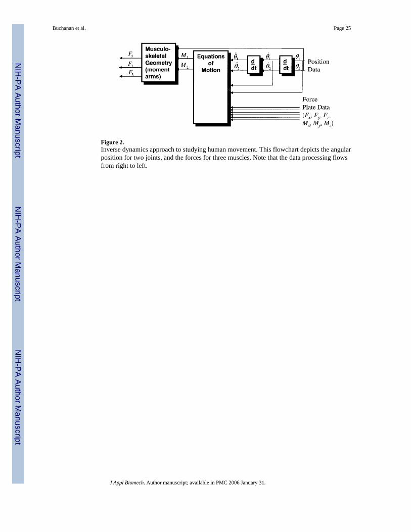
Figure 2.Inverse dynamics approach to studying human movement. This flowchart depicts the angularposition for two joints, and the forces for three muscles. Note that the data processing flowsfrom right to left.



NIH


NIH


NIH


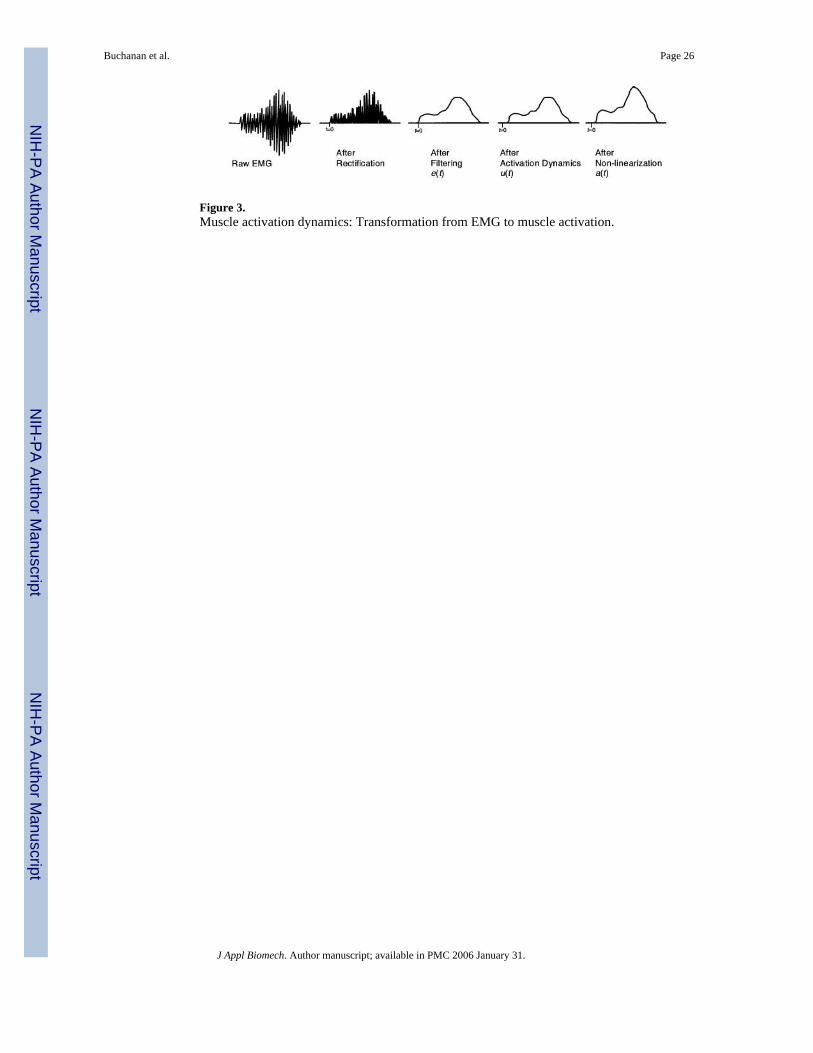
Figure 3.Muscle activation dynamics: Transformation from EMG to muscle activation.



NIH


NIH


NIH


Figure 4.Nonlinearization neural to muscle activation relationship: e(t) → a(t). (A) Dots represent datafrom Woods and Bigland-Ritchie (1983) for the biceps brachii for the isometric EMG-forcerelationship (demonstrating that other muscles showed a linear relationship), and the curvesrepresent Equation 11. In this scheme, a perfectly linear relationship would fall on line A= 0.As values for A increase, a nonlinear region is added for lower force levels (left side of the A-line), while linear relationships continue for higher values (right side of the A-line). Point Pmarks where these two curves join. (B) Equation 12 is used to accomplish the same goals. Herethe different shape factors, A, produce different curvature of the relationship. We limit A to befrom −3<A<0, where 0 is a straight line.



NIH


NIH


NIH


Figure 5.(A) Schematic of muscle-tendon unit showing muscle fiber in series with the tendon. Note thepennation angle, φ, of the muscle fiber relative to the tendon and that the total tendon length,ℓt, is twice that of the tendon on either end of the muscle fiber, ℓt/2. (B) Schematic of musclefiber with the contractile element and parallel elastic component. The nonlinear tendon stiffnessis given by k. The force produced by the contractile element, Fm, is a function of ℓm and νm,while the tendon force, Ft, is a function of ℓt. The total muscle fiber force, Fm, is the sum ofFAm and Fpm.



NIH


NIH


NIH


Figure 6.Normalized force-length relationship for muscle. Thick dark lines indicate maximumactivation, whereas the light thin lines are lower levels of activation. Note that the optimal fiberlength is longer as the activation decreases. In the figure, λ = 0.15, which means the optimalfiber length is 15% longer at zero activation.



NIH


NIH


NIH


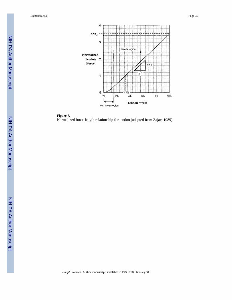
Figure 7.Normalized force-length relationship for tendon (adapted from Zajac, 1989).



NIH


NIH


NIH


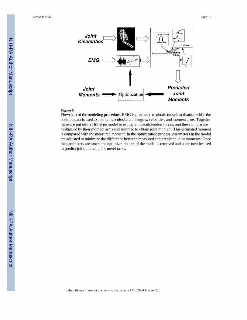
Figure 8.Flowchart of the modeling procedure. EMG is processed to obtain muscle activation while theposition data is used to obtain musculoskeletal lengths, velocities, and moment arms. Togetherthese are put into a Hill-type model to estimate musculotendon forces, and these in turn aremultiplied by their moment arms and summed to obtain joint moment. This estimated momentis compared with the measured moment. In the optimization process, parameters in the modelare adjusted to minimize the difference between measured and predicted joint moments. Oncethe parameters are tuned, the optimization part of the model is removed and it can now be usedto predict joint moments for novel tasks.



NIH


NIH


NIH


Figure 9.Output of the model described in the section on Model Tuning and Validation. Values for elbowmoment recorded experimentally are compared with those estimated by the model beforemodel parameter adjustment and after optimization or tuning.



NIH


NIH


NIH


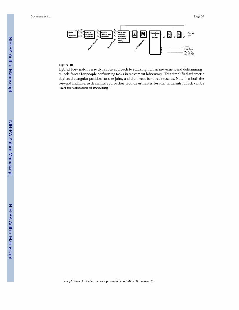
Figure 10.Hybrid Forward-Inverse dynamics approach to studying human movement and determiningmuscle forces for people performing tasks in movement laboratory. This simplified schematicdepicts the angular position for one joint, and the forces for three muscles. Note that both theforward and inverse dynamics approaches provide estimates for joint moments, which can beused for validation of modeling.



NIH


NIH


NIH


Figure 11.Typical results for predictions of knee joint moments from the calibrated Hybrid Forward-Inverse Dynamics approach: Crossover cut (left) and straight run (right). Thick line representsthe EMG-driven model results; thin line represents the inverse dynamics results. (Adapted fromLloyd & Besier, 2003)



NIH


NIH


NIH


Neuromusculoskeletal modeling: estimation of muscle forces and joint moments and movements from measurements of neural command

Documents