Neural-Symbolic Monitoring and Adaptation

Neural-Symbolic Monitoring and Adaptation

Alan PerottiUniversity of Turin

Email: [email protected]

Artur d’Avila GarcezCity University London

Email: [email protected]

Guido BoellaUniversity of Turin

Email: [email protected]

Abstract—metti esempietto diamond da slides.Runtime monitors check the execution of a system under scrutinyagainst a set of formal specifications describing a prescribedbehaviour. The two core properties for monitoring systems arescalability and adaptability. In this paper we show how RuleRun-ner, our previous neural-symbolic monitoring system, can exploitlearning strategies in order to integrate desired deviations withthe initial set of specification. The resulting system allows for fastconformance checking and can suggest possible enhanced modelswhen the initial set of specifications has to be adapted in orderto include new patterns.

I. INTRODUCTION

The expanding capabilities of information systems and otherframeworks that depend on computing resulted in a spectaculargrowth of the ”digital universe” (i.e., all data stored and/orexchanged electronically). It is essential to continuously monitorthe execution of data-producing systems, as well-timed faultdetection can prevent a number of undesired malfunctions andbreakdowns.A first requirement for runtime verification systems is scalability,as this guarantees efficiency when dealing with big data orsystems with limited computational resources. In [13] weintroduced RuleRunner, a novel rule-based runtime verificationsystem designed to check the satisfiability of temporal propertiesover finite traces of events, and showed how to encode it intoa standard connectionist model. The resulting neural monitorsbenefits from sparse form representation and parallel (GPU)computation to improve the monitoring performance.In this paper we tackle another crucial requirement for runtimemonitoring systems: adaptability. Adaptability overcomes thestandard classification approach to monitoring (where theverification task simply labels a trace as complying or not) andallows a monitor to adapt to new models or include unexpectedexceptions. In the Business Process area, a more flexibleapproach to monitoring is offered by model enhancement,where an initial model can be refined to better suit iterativedevelopment cycles and to capture a system’s concept drift. Itmay be the case that a user or domain expert would like tomodify the verdict of a monitoring task.In other scenarios, such as the implementation of directivesin big companies like banks, the task execution may differfrom the rigid protocol enforcement, due to obstacles (frombroken printers to strikes) or by adaptations to specific needs(dynamic resources reallocation). If the actual process executionrepresents an improvement in terms of efficiency, it is relevantto adapt the original process model in order to capture andformalise the system’s behaviour.We remark that this task differs from pattern discovery, as itdoes not infer an ex-novo model from the observed traces: thedesired feature is to be able to adapt the existing model. We

therefore propose a framework (visualised in Figure 1) basedon our RuleRunner system and integrating temporal logic andneural networks, for online monitoring and property adaptation.

Monitoring(Reasoning)

Adaptation(Learning)

actual != desired ?

Specification

Labelled Trace

Symbolic Encoding

Neural Encoding

Verdict

RuleRunner

Fig. 1: General framework

An initial temporal specification (i.e., one or more prop-erties) is provided as the expected behaviour of the systemin analysis. A runtime verification system, monitoring thatproperty, is then built. In Figure 1 we have stressed how in ourcase the encoding is decomposed in two steps. This is a pre-processing phase: the verification system is built once and canthen be used, at run time, to monitor traces. The monitoringprocess determines whether the pattern of these operationsviolates the specified property, providing binary verdicts. Thesub-workflow framed in a dashed line represents the monitoringtask as performed by RuleRunner. If the domain expert deemssome traces to be misclassified, the monitor enters an off-linelearning phase, where it modifies the encoded property in orderto modified the verdict for the traces marked as misclassified.The result of the learning process should be available both asa ready-to-use monitor and as a logical formula describing thenew adapted property, thus creating an iterative developmentcycle.

The paper is structured as follows: in Section II we presentbackground and related work, while in Section III we summariseour system, RuleRunner. In Section IV we outline the learningproblem and propose our solution. In Section V we concludethe paper with final remarks and directions for future work.

II. TECHNICAL BACKGROUND

A. Runtime Verification

The broad subject of verification comprises all techniquessuitable for showing that a system satisfies its specification(s).Correctness properties in verification specify all admissibleindividual executions of a system and are usually formulated insome variant of linear temporal logic ([14]). LTL properties arechecked against real systems through a process called modelchecking: more formally, given a model of a system and aformal specification, the model checking problem requires toexhaustively and automatically check whether the model meetsthe specification: however, software model checking is oftencomputationally hard [7], and infeasible when the model ofthe observed system is not known. A practical alternative isto monitor the running program, and check on the fly whetherdesired temporal properties hold: Runtime Verification [12],based on the concept of execution analysis, aims to be alightweight verification technique complementing other verifi-cation techniques such as model checking. Runtime monitoringis a valid option when the program must run in an environmentthat needs to keep track for violations of the specification, butthe source code is unavailable for inspection for proprietaryreasons or due to outsourcing. There exist several RV systems,and they can be clustered in three main approaches, basedrespectively on rewriting [16], [18] [10], automata [7], [6] [9]and rules [1] [13]. The aforementioned restrictions rule outseveral classical model-checking approaches, based on theconstruction of a model of the analysed system: for runtimeverification, one has to rely on the analysis of the so-calledtraces. Traces are streams of events, discretised according tosome temporal granularity: each discrete component of a traceis called cell.

B. Neural-symbolic Integration

(Artificial) Neural Networks [11] are computational modelsinspired by biological nervous systems and generally presentedas systems of interconnected ‘neurons’ which can computevalues from inputs. The Neural-Symbolic Integration areaprovides several hybrid systems that combine symbolical andsub-symbolical paradigms in an integrated effort. A milestonein neural-symbolic integration is the the Connectionist InductiveLearning and Logic Programming (CILP) system [5]. CILP’sTranslation Algorithm maps a general logic program P into asingle-hidden-layer neural network N such that N computesthe least fixed-point of P . In particular, rules are mappedonto hidden neurons, the preconditions of rules onto inputneurons and the conclusion of the rules onto output neurons.The weights are then adjusted to express the dependenceamong all these elements. The obtained network implementsa massively parallel model for Logic Programming, and itcan perform inductive learning from examples, by means ofstandard learning strategies.Borges et. al [3] proposed a new neural-symbolic system,named Sequential Connectionist Temporal Logic (SCTL) forintegrating verification and adaptation of software descriptions.This framework encodes a system description into a particularkind of network, namely NARX (Nonlinear AutoRegressivewith eXogenous inputs, [17]) and then a learning phase allowsthe integration of different knowledge sources. Properties to besatisfied are checked by means of an external model checking

tool (such as NuSMV [4]): if a property is not satisfied, thetool provides a counterexample that can be adapted with thehelp of an expert and be used to train the NARX network toadapt the model.

III. RULERUNNER

In a nutshell, RuleRunner [13] is a neural-symbolic systemwhere an LTL monitor is translated in a standard, feedfor-ward neural network. The monitor is initially computed asa purely symbolic system, composed by rules encoding theLTL operators, and then encoded in a standard recurrent neuralnetwork. As a result of the neural encoding, the monitoringtask corresponds to a feedforward recurrent activation of theneural network encoding the monitor.Given an LTL formula φ, RuleRunner is based on the parsingtree of φ: this is a tree where each node corresponds to anoperator (or observation) in φ, and each subtree to a subformulaof φ. For instance, the initial parsing tree for a∨3b is depictedin Figure 2(a).

⌃_

bTRUE

_

FALSE⌃

_

bTRUE

_

FALSE⌃

_

bTRUE

_

FALSEa a a

TRUE TRUE

TRUE

⌃_

b

⌃_

a

(a) (b)

Fig. 2: Example of parsing tree and labelling process

The monitoring task, for this structure, corresponds tolabelling the nodes with their truth values wrt. the currentobservations. The labelling proceeds bottom-up and it can bebased on a post-order visit of the parsing tree (Figure 2(b)).For instance, if b is observed, a is false and b is true. Theinformation that b is true can be used to infer that 3b is true,and the 3 node can therefore be labelled as true. The twolabels of a (false) and 3b (true) can be combined in the rootnode, according to the semantics of ∨, to finally label the rootnode as true and produce a final verdict: a ∨ 3b has beenverified by the observations.It is intuitive that each node in the parsing tree shouldencode the semantics of the corresponding operator; however,the runtime verification poses additional constraints, as theobservations trace can be accessed one cell at a time, and itis not possible to peek in the future nor to go back in thepast. To address the first limitation, RuleRunner assigns theundecided (?) truth values to formulae that require to accessthe suffix of the trace. This is a common approach in runtimeverification [2], used when it is impossible to give a binaryevaluation to a formula in the current cell: for instance if theformula is Xa, it is impossible to evaluate its value in the firstcell of a trace. However, RuleRunner is designed in such away that, when the end of the trace is reached, all truth valuesare binary.Concerning the second limitation, the truth values ofsubformulae are enriched with additional information aboutthe monitoring state. The enriched semantics of each LTL

operator is stored in what we called extended truth tables.As an example, the extended truth table for disjunction isvisualised in Table I.∨

B T ? FT T T T? T ?B ?LF T ?R F

∨L

T T? ?LF F

∨R

T T? ?RF F

TABLE I: Extended truth table for ∨

The right-hand side of Table I reports the three-valuedand decorated truth value table for ∨. ?L,?R and ?B read,respectively, undecided left, right, both. For example, ?L meansthat the future evaluation of the formula will depend on the leftdisjunct only, since the right one failed. An ?L truth value willforce the rule system to shift from the ∨B to the ∨L operator,in the following cells: ∨L is, in fact, a unary operator. Thisallows the system to ‘ignore’ future evaluations of the rightdisjunct and it avoids the need to ‘remember’ the fact that theright disjunct failed: since that information is time-relevant (theevaluation failed at a given time, but it may succeed in anothertrace cell), keeping it in the system state and propagating itthrough time could cause inconsistencies.The complete set of tables for logical operators is depicted inFigure 3.

!a

a ∈ statea ∉ state T

F

a (observation)

a ∈ statea ∉ state

T

F

^B ^L ^R

TT

T T

?R

T

F

?L

T

F

?B?L

?RT

F F F

F

F

F

F

F F

?

?

? ?

_R_L_B

TT

T T

?L

T

F

?R

T

F

?B ?L

?R

T

T

T

T T

FF

F

F F

?

?

? ?

WWM

?M

T

?M

T

F

T

FF

???

END � W XXM

?M

T

?M

T

F

F

FF

???

END � X

UA UB UL UR

?B

?L

?R

?ATT

TT

T T

F

F

F

F

?R

T

F

?L

T

F

?B ?B?L

?A ?AT

FFF

?B

?R

?A

?A

?AT

T

T FF

F F

F F F

?

?

?

?

? ?

END � U

?KT T

F

F

??

?K

F

?

⇤ END �⇤T F

F

?

?

T

?

?

END � ⌃⌃

Fig. 3: Extended truth tables

RuleRunner then translates every truth table as a smallneural network, creating one input neuron for each possible

truth value of the subformula(e), one hidden neuron for each cellin the truth table, and one output neuron for each possible truthvalue (true, false, undecided). The input-hidden connectionsimplement the compositions of cells in the truth table, and thehidden-output connections map each cell of the truth table ontoan output truth value. Figure 4 provides a visual example ofthe correspondence between extended truth tables and neuralnetworks: the example is simplified to a two-valued disjunction,for the sake of visualisation.

3 41 2

... ...

1 : true 2 : true

3 : true 4 : false

�

true false

�

falsetrue

true false

�true

true

�false

false

Fig. 4: (Two-valued) disjunction as network and truth table

The weights are computed using the CILP algorithm [8],which is proven to guarantee the following conditions:

C1 the input potential of a hidden neuron h can onlyexceed its threshold, activating h, when all the positiveantecedents of h are assigned the truth value true whileall the negative antecedents of h are assigned false.

C2 the input potential of an output neuron o can onlyexceed its threshold, activating o, when at least onehidden neuron h that is connected to o is activated.

Given an LTL formula φ, the final output of this encodingphase is a runtime monitor structured as the parsing tree for φ(see Figure 2) where each node corresponds to an LTL operatorand contains a neural network (e.g. Figure 4) computing thecorresponding extended truth table from (Figure 3). Whensuch a monitor is used to monitor a trace, the current cell’sobservations are fed to the neural monitor as input, and theconvergence of the feedforward-recurrent propagation in theneural monitor corresponds to the bottom-up labelling processon the formula parsing tree. In [13] we also showed how sparseform representation and parallel computation through GPU canspeed up the monitoring process.

IV. LEARNING AS PROPERTY ADAPTATION

A. The Learning Problem

In the introduction we have outlined our general frameworkfor integrating monitoring (reasoning) and adaptation (learning)within a single neural-symbolic system. We claim that thiskind of hybrid approach is required in many domains, spanningfrom Business Process Management (where it captures the ideaof concept drift) to Multi-agent systems (where autonomousagents can suggest improved solutions to a given task). As anexample, consider a security system built to detect consecutivelogin operations from the same user with no logout in between:

φ = login ⇒ X(!login ∪ logout). Now suppose the systemdetects a number of violations, in a given LAN, that thesecurity manager judges as false positives. For instance,that LAN could be a lab where users log in from differentdevices, or it could be a trustable section of the network. Itis reasonable that the security manager wants to maintainthe security system, but also to relax the formal property inorder to include logins from the given LAN, and thereforeavoid false positives and improve efficiency. Reclassifying atrace means demoting the relation between the observationsand the actual output while promoting the relation betweenobservations and expected output: it is, in fact, a supervisedlearning task. Therefore, wrt. the general framework depictedin Figure 1, the initial property is login⇒ X(!login∪ logout)and the traces are provided by the log of network operations,including logins and logouts. the learning phase modifies theencoded property in order to classify the consecutive loginsfrom the LAN area as non-violations: ideally, the resultingproperty is login⇒ X((!login ∨ LAN) ∪ logout).

The learning process has to be tackled by taking intoaccount both the temporal dimension of the monitoring andthe logical structure of the monitor. The intrinsic temporalnature of the monitoring process implies that learning thecorrect monitoring of a trace corresponds to learning a serieof classification instances, one for each cell of the trace.Furthermore, modifying the monitor when analysing a specificcell might alter the behaviour of the monitor on a previouslyanalysed cell, and learning attempts might result in conflictinginput-output pairs: we will solve this problem by consideringtemporary solutions as working hypotheses, and collecting setof said hypotheses before performing batch learning, so thatinconsistent options are ignored.Concerning the kind of formulae that can be learned, our neuralmonitors present a peculiar structure: on the one hand, we cantweak specific input-output relations within a single operator’struth table: we are therefore able to learn non-standard logicaloperators, such as the three-valued correspondent of NAND.This is an interesting feature, whereas several approaches arelimited to specific patterns or syntax citation needed!!!. On theother hand, recall that our neural monitors are based on parsingtrees, and the monitoring task correspond to leaves-to-rootmessage passing: in functional terms, learning implies alteringthe (semantics of the) property encoded in the monitor; instructural terms, it corresponds to modifying the weightsof some connections in the neural network. In our system,learning comes with a trade-off between preservation of theinitial monitor and learning capability: the balance dependson the degree of freedom we allow during learning. On theone hand, the initial monitor includes a set of propertiesconcerning consistence, truth-table interpretation, sparsity, andso on. On the other hand, if the network is fully connectedbefore the application of the learning algorithm, and everyconnection in both IH and HO is unconstrained, the learningalgorithm can rely on the full network in order to minimise theerror function. In this paper we opted for the former option -that is, locally constrained learning; we will discuss how thisallows to capture common property modification patterns, suchas constraint relaxations and exceptions (exploiting what wecalled contextual networks). If the exceptions in a set of tracesare based on complex temporal patterns that have no common

structure with the main property, it seems more reasonableto isolate those traces by standard monitoring and then use aminer to discover independent patterns, rather than trying tomerge property and exceptions, when they model syntacticallyand semantically different patterns.

B. Monitor Structure and Local Learning

In order to describe how to apply learning strategies toour system we need to analyse the structure of its neuralmonitors. We have mentioned in Section III how the supportingstructure for the monitors is the parsing tree of the encodedformula, where each node encode the operational semantics ofa precise operator. These nodes/subnetworks can be consideredas ‘flattened’ to ease the monitoring process (so that suiteslike Matlab can work with standard topologies), as depicted inFigure 5. However, for the learning process, we will considerthe subnetworks as organised in the original parsing tree. Notethat this double perspective does not require to rearrange thedata structure: the tree-based view can be achieved indexingthe subnetworks or following the recurrent connections.

4

1

2 3

...

...

...

H H H H

I I I

O OOO

H H H H

I I I

O OOO

1 2.........

H H H H

I I I

O OOO

3H H H H

I I I

O OOO

4

... ... ... ...

.........

Fig. 5: Flattened tree

It is also worth remarking how these subnetworks areindependent: computing A ∨ B depends on the truth valuesof A and B only: for instance, A and B may be complexformulae, and the process of computing their truth values doesnot affect the ∨ subnetwork; the final verdicts of A and Bare computed independently and propagated from the outputlayers of A and B to the input layer of A ∨B.

This structure is ideal for learning small adjustments tothe encoded property. For instance, if the encoded property isXXa ∧ 32(b Uc) and the goal is to learn traces generatedfrom XXa ∨32(b Uc), the only node in which learning isperformed is the one encoding the conjunction. In particular,switching from conjunction to disjunction consists in modifyinga few weights in the hidden-output layer in that neural network,as this corresponds to altering the truth values of some cells.

During learning, the weights (and thresholds) are modifiedaccording to the adopted learning strategies, like the perceptronadaptation algorithm or the backpropagation algorithm [15].However, different learning strategies just define the magnitudeof each weight update: the sign (increase/decrease) dependssolely on the nature of the problem. As an example, consider theneural network (encoding a disjunction) depicted in Figure 4,and suppose that it is used to learn the behaviour of a set oftraces. If the traces to be integrated are generated from an agentthat performs exclusively A or B, then the combination of Aand B will yield false: as a result, the learning algorithm willlower the weight of the 1 −→ true connection and increase theweight of the 1 −→ false connection. After the learning, the

hidden neuron 1, when firing, will propagate a signal towardsthe false output neuron. The resulting network and truth tablesare visualised in Figure 6.

3 41 2

... ...

1 : false 2 : true

3 : true 4 : false

�

true false

�

falsetrue

true false

�true

true

�false

false

Fig. 6: Network and truth table after the learning

Neurons and truth table can be easily re-labelled consultinga library of stored patterns: in the previous example, the learnedoperator is an exclusive or (⊕). Restricting the learning to thehidden-output weight matrix corresponds to training one-layernetworks (e.g. a layer of perceptrons), but we do not incurin the theoretical limits of linear separability, as every outputneuron implements a disjunction among the connected hiddenneurons (representing the cells in the truth table). For instance,A⊕B is not linearly separable, but h2 ∨ h3 is: and since thehidden neurons h2 and h3 correspond, respectively, to A∧!Band !A ∧ B, we obtain (A ⊕ B) ≡ ((A∧!B) ∨ (!A ∧ B)),which is a valid reformulation of the exclusive disjunction.

C. The Learning Approach

In the previous sections we have outlined several featuresand issues of possible learning approaches within our system;in this section we propose a particular learning framework. It isworth stressing that the kind of learning we want to implementis aimed at preserving the initially encoded property whileincluding/excluding new patterns: our final goal is to generateadapted monitors that, given a formula φ and a set of labelledtraces T , provide the minimal modification of φ that maximisesthe number of correctly classified traces in T .For this reason, we restrict the learning to single nodes ofthe parsing tree, corresponding to precise sets of rules (oneoperator). The advantages of this approach are several: firstof all, we prevent learning from disrupting the hierarchicalstructure of rules encoded by RuleRunner. Second, this approachpreserves the sparsity of the weight matrices in the neuralmonitor encoding the adapted formula. Third, local learningeases the extraction process, allowing to compute a symbolicdescription of the learned formula(e). The disadvantage of thisapproach is that we are constraining the learning capabilitiesof the system, limiting the search space to a syntacticalneighbourhood of the initial formula.The learning approach we propose is composed by two phases:first, local training sets are collected, and subsequently alearning strategy is applied on each training set.The starting point for learning is a monitor encoding an initialformula φ and a set of labelled traces. The labels of the traces

represent the desired monitoring verdict, which might notcorrespond to the actual output of the monitor encoding φ.There are two possible scenarios for the collection of thesetraces:

• A third-party system is observed and all of its trajec-tories are used as positive cases; the traces are thenverified against the initial monitor for φ.

• The initial monitor for φ labels all traces, and adomain expert modifies the verdict for the cases thathe wants the monitor to include/exclude.

Both the first phase (collection of the training sets) andthe second phase (actual learning) are split in a number ofindependent sub-phases, targeting specific nodes in the tree(that is, subnetworks of the neural monitor that encode specificsets of rules from the symbolic monitor). In each of these cases,the monitor is used to verify all labelled traces. In each cellof the trace, the first step is to compute the actual output: thisis depicted in Figure 7(a). The selected node is highlighted inred, and the information flow is visualised by blue arrows.

...

...

...

...

...

verdict

observation observation

...

...

...

...

...

label

(a) (b)

Fig. 7: Forward/backward propagation

Once the actual output is computed, it can be comparedwith the desired one, provided by the trace label. Since weare interested in modifying the highlighted node only, weneed to infer the desired output for that specific node, andwe compute it by a backwards propagation from the rootnode to the highlighted one (Figure 7(b)). So the monitoris used to propagate (forward) the actual global output and, ifit differs from the expected label, to propagate (backward) thelocal expected output for the highlighted node. Note that thebackward propagation of the expected output corresponds toabduction.At this point, we do have the couple of actual input and desiredoutput for the selected node: the former was computed in themonitoring step, while the latter was obtained by backwardspropagation, starting from the desired label. We store this coupleof values, force the expected output in the selected node, andmove to the next cell. We do so for the following reasons:

• We know that by forcing the output of the selected nodeto match the desired one, the remaining forward propa-

gation will produce the expected label, thus allowing -if necessary - to proceed with the monitoring. Thus weuse the input-output behaviour as a working hypothesisin order to proceed with the monitoring/learning.

• We store the actual input/desired output as part ofthe training set for the selected node. By doing so,we postpone all actual learning to a subsequent phase,where it can be applied to a whole training set (batchapproach).

...

_

...

...

...

...

Input Output... ...

Input Output

Input Output... ...

Input Output

Input Output... ...

Input Output

Input Output... ...

Input Output

Input Output... ...

Input Output

Fig. 8: Collecting local training sets

At the end of this phase, for each node in the initial monitora training set has been built (Figure 8). Note that we simplydefined each element as an input-output pair, but in fact inputand output are activation patterns on the input/output layer ofthe selected node. In the second phase, learning strategies canbe exploited to make each subnetwork match the input-outputbehaviour represented by the corresponding local training set;all these training tasks are independent and can be run inparallel.

D. Contextual Subnetworks

So far we focused on learning tasks where the desiredbehaviour was an alteration of the encoded property, commonlyby means of a relaxation of some connective. However,it may be the case that the desired behaviour depends onadditional observations that do not belong to the initialformula. This happens, for instance, with exceptions, wherea specific case can be isolated and exempted from a general rule.

A neural monitor NNφ, as it is, is not suitable for learningbehaviours including new observations, as everything whichis not included in the original property is filtered. This isreasonable for the ‘pure monitoring’ phase, as the size ofobservations provided by the observed system may be arbitrarilybig wrt. the few observations to be monitored. However,when adapting the monitor in order to learn to re-classifytraces, taking new observations into account may be necessary.A simple example for this particular issue was provided inSection ??, concerning the security domain: the initial propertydid not include details about the LAN, so that information wasinitially ignored by the monitor.In structural terms, the neural monitor may lack the actualinput neurons necessary to be aware of some observations. Inorder to overcome this limitation, the topology of the neuralnetwork has to be modified in order to detect the desired

observations and be able, through learning, to connect themwith the rest of the network, so that the occurrence of the newobservation influence the overall semantics of the monitor. Wecall contextual subnetwork for a (CSa) the subnetwork addedto the initial neural monitor in order to take into account theoccurrence of an observation a.As a minimum requirement, CSa must include an input neuronlabelled a, so that the activation of the neuron corresponds tothe occurrence of a in the current cell. However, this is notsufficient in our convergence-based approach, as the monitoringof a subformula requires several feed-forward propagations inthe neural monitor, and a has to be ‘remembered’ throughoutthis phase. We adopt the same technique we used for theobservations belonging to the initial formula: persistence clauses(see Section ??). The minimal CSa for an observation a istherefore visualised in red in Figure 9.

R..R..x

FS..

R..R..x

FS..

a

a

NN for � NN for �

Fig. 9: Minimal contextual subnetwork for a

CSa corresponds to the simple logic program:

a⇒ a

However, as we have observed in the previous subsections, itis often the case that the occurrence of an observation and itsimpact on the desired final verdict belong to two different cells;in order to satisfy this need of through-time persistence, wepropose a second type of contextual subnetwork which remem-bers whether a given observation o was always/sometimes truein the past. This extended contextual subnetwork, highlightedin Figure 10, corresponds to the following logic program:

a ⇒ a

a ⇒ 3a

3a ⇒ 3a

(2a ∧ a)⇒ 2a

The first clause corresponds to the minimal contextual network,and it is used to link the occurrence of a with the output patternof the neural monitor. The second and third clauses model theexistential occurrence of a: if a is observed, then 3a holdsfrom that cell; if 3a holds, it is maintained in the future cells.The fourth clause model the universal existence of a: as longas a is observed, 2a holds.

R..R..x

FS..

R..R..x

FS..

a

a

<>a

(or)

<>a

[]a

(and)

[]a

NN for � NN for �

Fig. 10: Extended contextual subnetwork for a

Specific contextual networks can be built in order to meetspecific needs; in Section ??, for instance, we exploit a delay-unit contextual network that allows us to take into accountexceptions that occurred in the previous cell.Contextual networks provide additional inputs for the neuralmonitor, but are initially disconnected from the neural monitorand have no impact on the monitoring process; it is necessary toapply a learning strategy to connect the main neural monitor andthe built contextual networks, so that the occurrence of excep-tions impacts on the monitoring verdict. The general approachpresented in Chapter ?? can also be used to learn exceptions,e.g. unpredicted patterns that involve atoms (observations) notincluded in the original formula. We use precisely the same setof algorithms, with one single difference: the focus node is notselected on the tree of the original monitor, but added ex novo,connecting the neural monitor with a contextual network. Theapproach is sketched in Figure 11: in any edge from a node A toa node B, a new dummy node, called Graft in figure, can beinserted. Initially the node computes a left-projection function,so that it simply propagates the output of the B node as inputto the A node. A contextual network (see Subsection IV-D) isadded as right subnode of the Graft. The contextual networkcan store arbitrary information about a given atom, or set ofatoms, not previously included in the initial formula (which themain tree is monitoring). In the simplest case, the contextualsubnetwork for a given observation x simply detects whether xholds in the current trace. Using the Graft node as focus nodein the learning process allows the monitor to take into accountthe information computed and stored in the contextual nodeand to let it influence the verdict of the adapted monitor, if thisimproves the monitoring accuracy. The richness of symbolicalinformation about the evaluation status of all subformulae ofthe currently monitored property allows us to decide where tograft the contextual node with surgical precision, measuring itsimpact on different nodes in independent tests.

A

B

...

... ...

...

A

B

...

... ...

...Graft

Context

Fig. 11: Grafting a contextual subnetwork to a monitoring tree

E. Example

Let us provide a first trivial example of our learningframework. The first, detailed example involve Ma∨b asinitial monitor, a ∧ b as the formula to be learned, anda b END/a END/b END and END as traces.The domain expert labels the traces as follows: a b ENDas SUCCESS, a END as FAILURE, b END asFAILURE, and END as FAILURE.The monitoring (with Ma∨b) starts. Trivially, the misclassifiedtraces are t2 and t3, where in the first (and only) cell Ma∨b

yields SUCCESS and the given label is FAILURE. Theinitial accuracy is therefore 50%.In these two cases, for all nodes in Ma∨b, Algorithm ??invokes the Repair(·) function in Algorithm ??. Let us selectthe focus nodes in a top-down manner, in order to explain thebackpropagation gradually.

• If the focus node is TOP , the backpropagation inRepair(·) stops instantly. In both cases, the ac-tual output is SUCCESS and the expected one isFAILURE, so an adaptation is possible. In both casesthe input of the TOP node is simply [a ∨ b]T , so thecouple {[a ∨ b]T , FAILURE} is returned.After going through the two cases, the nodeTOP in Ma∨b is actually modified using {[a ∨b]T , FAILURE} as a training set. This causes theinitial rule set

[a ∨ b]T e7−−−→ SUCCESS

[a ∨ b]? e7−−−→ REPEAT

[a ∨ b]F e7−−−→ FAILURE

to become

[a ∨ b]T e7−−−→ FAILURE

[a ∨ b]? e7−−−→ REPEAT

[a ∨ b]F e7−−−→ FAILURE

So the system displays

[a ∨ b]F e7−−−→ SUCCESS : FAILURE

The adapted monitor is used to label the traces inT , and it produces the verdict FAILURE to all ofthem (accuracy: 75%). Trivially, since in this particularcase we only had failure-to-success cases, the monitorlearned a constant function. It should be evident to theuser that, in this case, the answer is trivial.

• If the focus node is ∨, both on t2 and t3 the Repair(·)function invokes the Abduce(·) function to migratefrom the root node TOP to the focus node ∨. As inall cases in this example, in TOP the actual outputis SUCCESS and the expected one is FAILURE.The only rule producing FAILURE is [a∨b]F e7−−−→FAILURE, and [a∨ b]F is an unmatched literal thatrefers to the subtree where the focus node is. Abduce(·)returns [a∨b]F and Repair(·) makes a recursive call onthe ∨ node with expected output [a∨b]F . The informaldescription of this step is if I want the monitoring tofail, then the disjunction node must produce [a ∨ b]F .In the recursive call on the ∨ node, the current nodeis the focus one. The current output, both for t2 andt3, is [a ∨ b]T , while the expected one is [a ∨ b]F : thealgorithm forces [a ∨ b]T as output for the disjunctionnode. In the case of t2, the input is R[a∨b]B , [a]T , [b]F ,so the algorithm returns {{R[a∨b]B , [a]T , [b]F }, {[a∨b]F }}. For t3, the input is R[a∨b]B , [a]F , [b]T and thealgorithm returns {{R[a∨ b]B , [a]F , [b]T }, {[a∨ b]F }}.In both cases, the TOP node recomputes its output:since the initial state now contains [a ∨ b]F instead of

[a ∨ b]T , in both cases FAILURE is inferred. Thefirst phase terminates and the disjunction node in theinitial monitor is modified according to the collectedtraining set:

{{R[a ∨ b]B , [a]T , [b]F }, {[a ∨ b]F }}{{R[a ∨ b]B , [a]F , [b]T }, {[a ∨ b]F }}

Since there are no inconsistencies in the training setthe modified rules are

R[a ∨ b]B , [a]T , [b]F e7−−−→ [a ∨ b]T : [a ∨ b]F

R[a ∨ b]B , [a]F , [b]T e7−−−→ [a ∨ b]T : [a ∨ b]F

The adapted monitor is used to label the traces in T ,obtaining an accuracy of 100%. It is worth notinghow the adapted rule correspond to the different cellsbetween the (two-valued) truth tables of disjunctionand conjunction. In this simple case, the learned nodedoes not perfectly match the three-values conjunctionschema, as the learning framework wasn’t presentedwith examples of conjunctions involving undecidedsubformulae; the conjunction schema is the bestapproximation, nonetheless, and it would not diminishthe accuracy on this example’s simple monitor overthe set of traces T .

• If the focus node is a, the Abduce(·) function needsto be invoked twice in order to reach the focus nodefrom the root one. When analysing t2, the startingpoint is Repair(·) on node TOP with expected outputFAILURE. The following recursive call (as describedin the previous case) is Repair(·) on node ∨ withexpected output [a∨b]F . The input is R[a∨b], [a]T , [b]F .Out of all rules in the ∨ node, only those producing[a ∨ b]F are initially selected:

R[a ∨ b]B , [a]F , [b]F e7−−−→ [a ∨ b]F

R[a ∨ b]L, [a]T e7−−−→ [a ∨ b]F

R[a ∨ b]R, [b]F e7−−−→ [a ∨ b]F

The second and third rules are excluded since R[a∨b]Land R[a∨ b]R (respectively) do not belong to the inputof the current node. Only R[a∨b], [a]F , [b]F e7−−−→ [a∨b]F remains, and the literal concerning the focus sub-tree, [a]F , is selected. The last recursive call is thereforeRepair(·) on node a with expected output [a]F . TheRepair(·) function returns {{R[a], a}, {[a]F }}. Theoutput of node a is forced to [a]F , and consequentlythe output of nodes ∨ and TOP become, respectively,[a ∨ b]F and FAILURE.On t2, the recursive calls are the same, but the outputof node a is [a]F in this case (since a is not observed int3): when Repair(·) is called on node a with expectedoutput [a]F , since the actual output matches the desiredone, Repair(·) returns an empty set.The learning algorithm modifies the node a as follows:

R[a], ae7−−−→ [a]T : [a]F

The resulting monitor has an accuracy of 75%. Whatthe framework did, in this case, was to cast a to a

constant (false) function, as this correctly classifiest2 as FAILURE; however, there is no way thatmodifying the rules of a can cause the monitor toclassify t3 as FAILURE (as b holds and the non-anodes are unmodified).

• The case for b is specular; this concludes the currentexample.

Another interesting example is trying to adapt (aUb) to 3b(Table III): in this case we haven’t modified one operator, butused a different syntax to express a similar property (recallthat (>Ub) ≡ 3b).

Node Accuracy Learned RulesInitial accuracy: 49.4%

a 100.0% R[a], !ae7−−−→ [a]F : [a]T

b 100.0% R[b], !be7−−−→ [b]F : [b]?

(aUb) 100.0%

R[(aUb)]A, [a]F , [b]F

e7−−−→ [(aUb)]F : [(aUb)]?AP

R[(aUb)]R, [b]F ]

e7−−−→ [(aUb)]F : [(aUb)]?BP

R[(aUb)]B , [a]F , [b]T

e7−−−→ [(aUb)]F : [(aUb)]T

R[(aUb)]L, [a]F e7−−−→ [(aUb)]F : [(aUb)]T

R[(aUb)]B , [a]F , [b]F

e7−−−→ [(aUb)]F : [(aUb)]?LP

TOP 49.4% ∅

TABLE II: From (aUb) to 3b

Since the SUCCESS −FAILURE proportion is almostfair (49.4%), in this case the TOP node was not modified,preserving the initial accuracy. It is interesting to see how thelearning procedure produced three locally-modified monitorsthat perfectly classify the given traces.

• In the (aUb) node, the learning algorithm adapteda set of rules (recall how rich the evaluation tablesfor U are). The first, second and fifth rules take intoaccount situations where b is false, forcing the resultfrom false to undecided: since in fact the traces arelabelled according to the formula 3b, a failure of bjust requires the whole monitoring to proceed. Thesecond rule forces the monitor to yield a true resultwhen b is observed, ignoring the fact that a failed:this mirrors the fact that in 3b a is irrelevant. Thethird rule, similarly, expresses the fact that when onlythe monitoring of a is pending (and this means that balready succeeded), the monitoring of the U formulaterminates with a positive verdict.

• In the b node the learning process produced a singleupdated rule: R[b], !b e7−−−→ [b]F : [b]?. This may lookweird, as it is a mere observation being assignedan undecided truth value. In fact, as long as b isnot observed, [b]? is inferred, and this causes thesuper-formula (aUb) to iterate on the following cell.If a is not observed, the until simply switches fromthe A to the B sub-states (see Section ??): the systemhas just found another way to ignore a. If eventuallyb is observed, [b]T and [(aUb)]T are inferred, causingthe monitoring of the trace to produce a SUCCESSverdict. If b is never observed, the (aUb) formula

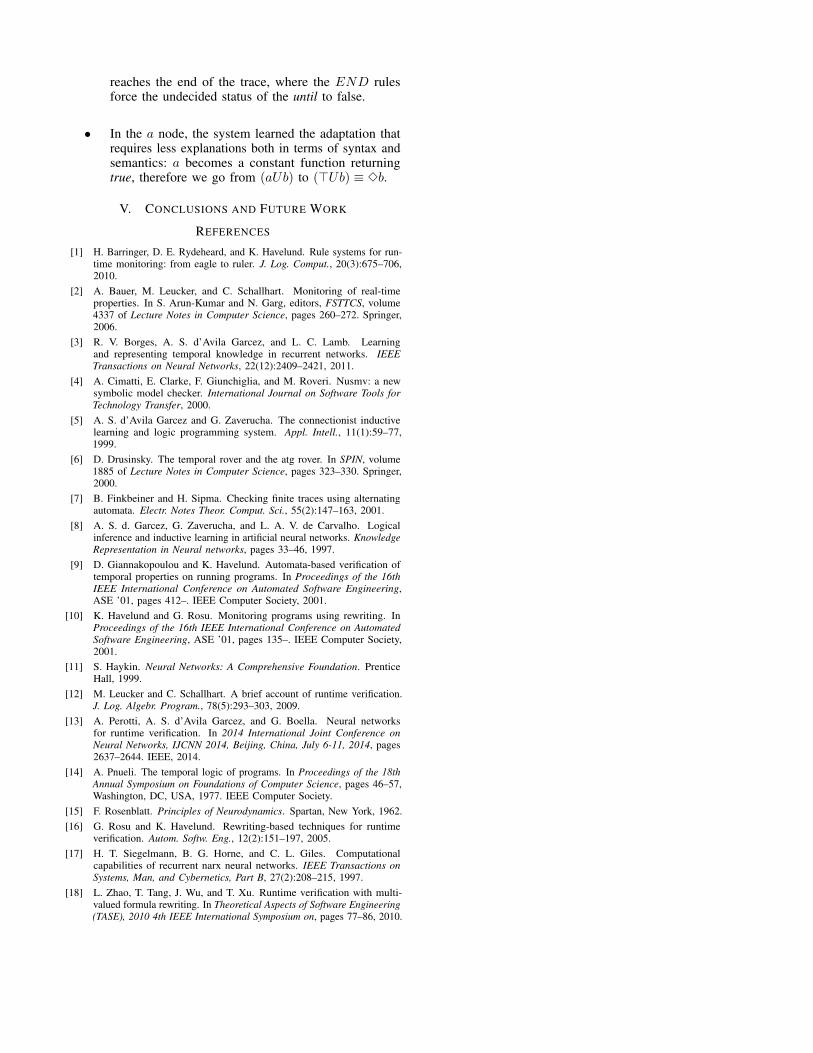
reaches the end of the trace, where the END rulesforce the undecided status of the until to false.

• In the a node, the system learned the adaptation thatrequires less explanations both in terms of syntax andsemantics: a becomes a constant function returningtrue, therefore we go from (aUb) to (>Ub) ≡ 3b.

V. CONCLUSIONS AND FUTURE WORK

REFERENCES

[1] H. Barringer, D. E. Rydeheard, and K. Havelund. Rule systems for run-time monitoring: from eagle to ruler. J. Log. Comput., 20(3):675–706,2010.

[2] A. Bauer, M. Leucker, and C. Schallhart. Monitoring of real-timeproperties. In S. Arun-Kumar and N. Garg, editors, FSTTCS, volume4337 of Lecture Notes in Computer Science, pages 260–272. Springer,2006.

[3] R. V. Borges, A. S. d’Avila Garcez, and L. C. Lamb. Learningand representing temporal knowledge in recurrent networks. IEEETransactions on Neural Networks, 22(12):2409–2421, 2011.

[4] A. Cimatti, E. Clarke, F. Giunchiglia, and M. Roveri. Nusmv: a newsymbolic model checker. International Journal on Software Tools forTechnology Transfer, 2000.

[5] A. S. d’Avila Garcez and G. Zaverucha. The connectionist inductivelearning and logic programming system. Appl. Intell., 11(1):59–77,1999.

[6] D. Drusinsky. The temporal rover and the atg rover. In SPIN, volume1885 of Lecture Notes in Computer Science, pages 323–330. Springer,2000.

[7] B. Finkbeiner and H. Sipma. Checking finite traces using alternatingautomata. Electr. Notes Theor. Comput. Sci., 55(2):147–163, 2001.

[8] A. S. d. Garcez, G. Zaverucha, and L. A. V. de Carvalho. Logicalinference and inductive learning in artificial neural networks. KnowledgeRepresentation in Neural networks, pages 33–46, 1997.

[9] D. Giannakopoulou and K. Havelund. Automata-based verification oftemporal properties on running programs. In Proceedings of the 16thIEEE International Conference on Automated Software Engineering,ASE ’01, pages 412–. IEEE Computer Society, 2001.

[10] K. Havelund and G. Rosu. Monitoring programs using rewriting. InProceedings of the 16th IEEE International Conference on AutomatedSoftware Engineering, ASE ’01, pages 135–. IEEE Computer Society,2001.

[11] S. Haykin. Neural Networks: A Comprehensive Foundation. PrenticeHall, 1999.

[12] M. Leucker and C. Schallhart. A brief account of runtime verification.J. Log. Algebr. Program., 78(5):293–303, 2009.

[13] A. Perotti, A. S. d’Avila Garcez, and G. Boella. Neural networksfor runtime verification. In 2014 International Joint Conference onNeural Networks, IJCNN 2014, Beijing, China, July 6-11, 2014, pages2637–2644. IEEE, 2014.

[14] A. Pnueli. The temporal logic of programs. In Proceedings of the 18thAnnual Symposium on Foundations of Computer Science, pages 46–57,Washington, DC, USA, 1977. IEEE Computer Society.

[15] F. Rosenblatt. Principles of Neurodynamics. Spartan, New York, 1962.[16] G. Rosu and K. Havelund. Rewriting-based techniques for runtime

verification. Autom. Softw. Eng., 12(2):151–197, 2005.[17] H. T. Siegelmann, B. G. Horne, and C. L. Giles. Computational

capabilities of recurrent narx neural networks. IEEE Transactions onSystems, Man, and Cybernetics, Part B, 27(2):208–215, 1997.

[18] L. Zhao, T. Tang, J. Wu, and T. Xu. Runtime verification with multi-valued formula rewriting. In Theoretical Aspects of Software Engineering(TASE), 2010 4th IEEE International Symposium on, pages 77–86, 2010.