Neural Network Survival Analysis

Faculty of Sciences

Department of Applied mathematics and computer science

Neural Network Survival Analysis

Yanying Yang

Promoter: Prof. Dirk Van den Poel

Co-Promoter: Prof. Els Goetghebeur

Master dissertation submitted to obtain the degree of

Master of Statistical Data Analysis

Academic year 2009 - 2010

The author and the promoters give permission to consult this master dissertation

and to copy it or parts of it for personal use. Each other use falls under the

restrictions of the copyright, in particular concerning the obligation to mention

explicitly the source when using results of this master dissertation.

June 28, 2010

Gent, Belgium

The Promotor

Prof. Dirk Van den Poel

The Co-promotor

Prof. Els Goetghebeur

The author

Yanying Yang

i

Preface

I wish to thank my promoter Prof. Dirk Van den Poel who gave me the

opportunity to take this thesis subject and guided me to pave through these

uncharted areas. My thanks specially go to my co-promoter -Prof. Els

Goetghebeur. Her suggestions and advices finally made me grasp the key to

the gate of hope for my thesis.

I'd also like to thank Jozefien Buyze. Thank you for sharing knowledge with me

and encouraging me when I ran into problems that look overwhelming.

Also many thanks go to my friends and family for keeping me looking

forward, particularly to my one year old. Although you cannot talk yet, your

smile is the most powerful source of strength for me. I also like to thank my

husband for sharing the burden on both my thesis work and house-keeping.

Thank you all!

Aug. 28, 2010

Gent, Belgium

ii

Summary

In this study, we analyzed a data set from real commercial data on the purchase

behaviors of 168 customers to predict the next purchase time. The data were grouped

to the training set and test set, and analyzed by a piecewise standard Cox PH model, a

piecewise marginal Cox model and the PLANN neural network approach.

The effects of the following five factors were studied: the previous purchase interval,

the type of a customer, the region and size of the city where a customer lives, and the

season of the last purchase. The three models (two Cox's PH models and the ANN

model) were used to predict the survival of the test set. In total eight subgroups of the

test set were selected and their predicted survivals were compared to the KM survival

estimates. The comparison shows that the ANN methods displayed similar

predictability performance with that of the piecewise standard Cox PH model. Thus,

the hypothesis that the ANN method is superior to the conventional Cox's PH models

does not valid.

The study reveals the following patterns in the purchase behaviors: 1) the next

purchase interval approximately proportional to previous interval， while the output

of the marginal Cox model indicates that for a customer the marginal effect of the

previous interval on the next purchase interval is not significant. 2) The purchase

interval of a customer living in big or medium city is not significant different with

that of a customer in small or tiny city. 3) The customers whose types are ‘catering’ or

‘horeca’ have similar purchase trends and have shorter purchase periods than that of

other type customers. The ‘particulier’ customers tend to do their next purchase later.

For the retail customer, no distinct results were shown. 4) The customers in Waals

Brabant or Vlaams Braban tend to do their purchases after 7 days, while the

customers in West Vlaanderen, Luxemburg and Limburg would like to purchase

earlier than those in the other customers. 5) Customers tend to do the next purchases

earlier during Apr. to Aug., and postpone the next purchases in Dec.

iii

Contents

1 Introduction ............................................................................................................................... 1

2 Data set and Method ................................................................................................................. 3

2.1 Data set .......................................................................................................................... 3

2.1.1 Original data set and variables .......................................................................... 4

2.1.2 Analyzed data set .............................................................................................. 4

2.1.3 Training and Test data sets ................................................................................ 5

2.1.4 Factors to be analyzed ....................................................................................... 6

2.2 Survival Analysis .......................................................................................................... 6

2.2.1 Theory of survival analysis ............................................................................... 7

2.2.2 Covariates and their PH Assumption Assessment ........................................... 10

2.2.3 Piecewise Cox PH models............................................................................... 13

2.2.4 Prediction of survival probabilities of the test set ........................................... 14

2.3 Neural network survival analysis ................................................................................ 16

2.3.1 Theory of neural network survival analysis .................................................... 16

2.3.2 Transformation of the data .............................................................................. 19

2.3.3 ANN Model ..................................................................................................... 20

2.3.4 Calculation of hazard ratio and survival probability ....................................... 22

2.4 Comparison ................................................................................................................. 23

2.4.1 Subgroups to be compared .............................................................................. 23

2.4.2 Comparison of hazard ratios and survival probabilities .................................. 23

3 Results ..................................................................................................................................... 24

3.1 Hazard ratios ............................................................................................................... 24

3.2 Factor effects ............................................................................................................... 25

3.3 Predictability of the three models ............................................................................... 30

4 Discussion and Conclusion ..................................................................................................... 33

4.1 Conclusion .................................................................................................................. 33

4.2 Selection of the covariates .......................................................................................... 33

4.3 Comparison of methods .............................................................................................. 34

5 References ............................................................................................................................... 37

6 Appendix ................................................................................................................................. 39

A-1 Original and analyzed data set .................................................................................... 39

A-2 Proportional Hazard Assumption Check. .................................................................... 46

A-3 Introduction: Artificial Neural network (ANN) .......................................................... 51

1

1 Introduction

Survival analysis can be performed to explore the occurrence of some events such as

deaths after a treatment in a population of subjects. Some regression models are

developed to explore the relationship between survival explanatory variables and

predict outcomes. The Cox's proportional hazards model (Cox’s PH model) is one of

the most widely applied models. For this model, the hazard ratio of a group to a

baseline group is assumed to be constant through the observe time. If the PH

assumption does not hold, some techniques must be applied such as combination of

the subgroups of a variable, a stratified model, an extended model with time

dependent variables, and a piecewise model where the PH assumption is satisfied

within each time span.

Despite the existence of the aforementioned techniques, the PH assumptions might

remain untenable in some situations. In addition, modeling the underlying

relationships of multivariate data implies a definition of a correct functional

relationship among the considered variables. These variables must be expressed by a

finite number of parameters, and the determination of these variables must be based

on prior information of the phenomena understudy.

To address these limitations, several methods employing the artificial neural network

(ANN) have been suggested in survival analysis. The ANN can be employed to

directly predict the survival times, or to predict the survival and hazard. It can also be

used to extend the Cox’s PH model. Some of these ANN survival analysis methods

require modifying data representation to model censored survival data in the neural

network.

The main merit of neural networks is that they are capable of dig information hidden

in data without constraints on the properties of the data. For this reason, a ANN model

is generally regarded as one of the most flexible models, and is suitable for non-linear

multivariate problems. A non-linear predictor can be fitted implicitly by an ANN

model, and the effects of the covariates are allowed to vary arbitrarily but smoothly

2

over time in an ANN model. However, major criticism to this method lies in its ‘black

box’ way of handling the data, which provides a fuzzy, ambiguous model and cannot

be expressed explicitly. Due to this reason, both the model and the impact of

individual covariates are lack of easy interpretations. In addition, the randomness of

the initial values used to train the neural network makes the method unstable

sometimes.

ANN-based approaches have been employed in many studies and the prediction

performance has been compared with some traditional regression models.

Theoretically, the ANN method is more effective in analysis complex data with

non-linear covariates, high order interaction among covariates, and time-dependent

covariates than traditional regression methods. However, not all studies show that

neural network methods are superior to a properly fitted traditional regression method

In this work, we will analyze a data set from real commercial data on the purchase

behavior of 168 customers. The purpose of this study is to investigate the factors that

contribute to the time of next purchase of a customer. These factors are the season of

the last purchase, the type of a customer, the region where a customer lives, and the

previous purchase interval. The methods employed in this work are: the standard

Cox’s PH model, the marginal Cox’s PH model, and an ANN model. The prediction

performance of all these three models will be compared. We will also verify the basic

hypotheses on applying neural network in survival analysis: a neural network model is

superior to the Cox’s PH model in predicting the survival for a complex data set.

Because the PH assumption holds within several time periods, a piecewise standard

Cox’s PH model and a piecewise marginal Cox’s PH model were fitted. In the

standard Cox’s PH model, the observations belonging to a same customer are

assumed to be independent. In the marginal model, the correlation among recurrent

events of a subject is adjusted by using the robust estimation method. But the

marginal model does not account for the occurrence order of recurrent events.

The neural network survival analysis approach used in the study is the partial logistic

artificial neural network (PLANN) regression approach reported by Elia Biganzolil

3

and Patrizia Boracchi et al. For each subject, the output is the estimated conditional

probability of the occurrence of an event as a function of the time interval and

covariate patterns. A survival function can be estimated based on the hazard. The

PLANN approach allows for a joint modeling of time, the continuous and categorical

explanatory variables in a multi-layer perception model, but without proportionality

constraints. This approach allows a straightforward modeling of time-dependent

explanatory variables.

The data sets and methods are introduced in Chapter 2. The results of the three fitted

models are given in Chapter 3. The results are first interpreted and then compared

with each other. The prediction performance of the ANN model is demonstrated to be

superior to the Cox’s PH models. The results are discussed in Chapter 4.

2 Data set and Method

This paper measured the time interval between two neighbored purchase records of

one customer, which is called visit interval. The effects of the following five factors

were explored: 1) previous purchase interval, 2) customer type, 3) region a customer

lives in, 4) size of the city a customer lives in and 5) season.

The data set was randomly divided to a training set and a test set. The training set was

used to fit a standard Cox PH model and a marginal Cox PH model, and train a neural

network model. Based on the output of three models, survival functions of the test set

were estimated and compared.

2.1 Data set

The original data set contained purchase records of 169 customers, types of customers,

and the post code of city where a customer comes from. The repeated visits of one

customer in the same day were recorded as one observation in the analyzed data. The

records of customer No. 160 were suspected to be outliers and deleted. The obtained

4

data set was referred as the analyzed data set and randomly grouped into training and

test data set.

In the analyzed data set, the observation time was set to from January 2, 2003 to

March 31, 2009. 119 observations were censored. In addition, all purchase intervals

longer than 42 days were also censored as 42 days. The censor was assumed to be non

informative censor and the censor rate was 0.76%.

2.1.1 Original data set and variables

The original data set included 126,433 purchase records and four variables: 1)

cust_no , which is the indices of 169 customers, 2) visitdate2 , which records the

purchase date in SAS date format, 3) type, which shows four types of customers, 4)

code_post , which indicates the post code of city where a customer comes from.

The purchase records began from Jan.2, 2003 to Feb.16, 2005, and ended from Jan.9,

to Apr.9, 2009. The mean follow up time was 2062 days. The mean visit interval was

3 days. The starting time, end time, follow up time, visit frequency and visit intervals

of each individual customer are analyzed in Appendix A1.1.

2.1.2 Analyzed data set

Deleting repeated purchase records

About 85% customers had repeated purchase records in the same day in the original

data set. The repeated purchases occurred for many reasons, and were recorded as

multiple different observations in the data set. But these observations were not related

with a new purchase goal. So the repeated visits of one customer in the same day were

recorded as one observation in the analyzed data.

After deleting repeated visit records, the new data set had 44049 observations, and the

mean purchase interval was 8.6 days.

The properties of purchase behavior of each individual customer, including the follow

up time, the visit frequency, the mean, the maximal and the minimal visit intervals,

were analyzed and showed in Appendix A1.2.

5

Deleting outlier records

According to the visit frequency and mean purchase interval, some observations were

suspected to be outliers and explored in Appendix A1.3. The associated records of the

customer No. 160 were deleted.

In the original data set, the customer with cust_no 160 had more than 60% of the visit

observations and extremely small mean visit intervals (0.025 days). After deleting the

repeated visit records of customer 160, he still had extremely large visiting

frequencies and small mean visit intervals (1.5 days).

Defining the observe time and censoring

The observation time was set to from January 2, 2003 to March 31, 2009. All

observations which occurred after the end date were regarded as censored data. This

operation made 119 observations censored data.

In addition, all purchase intervals longer than 42 days were also censored as 42 days.

The censor rate was 0.76%.

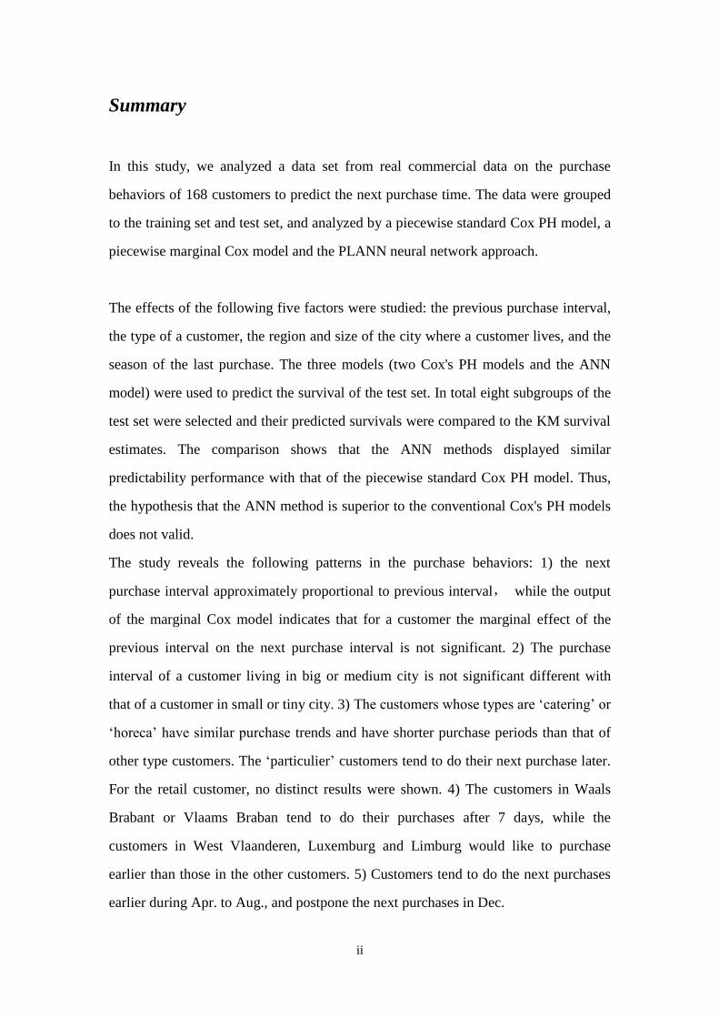
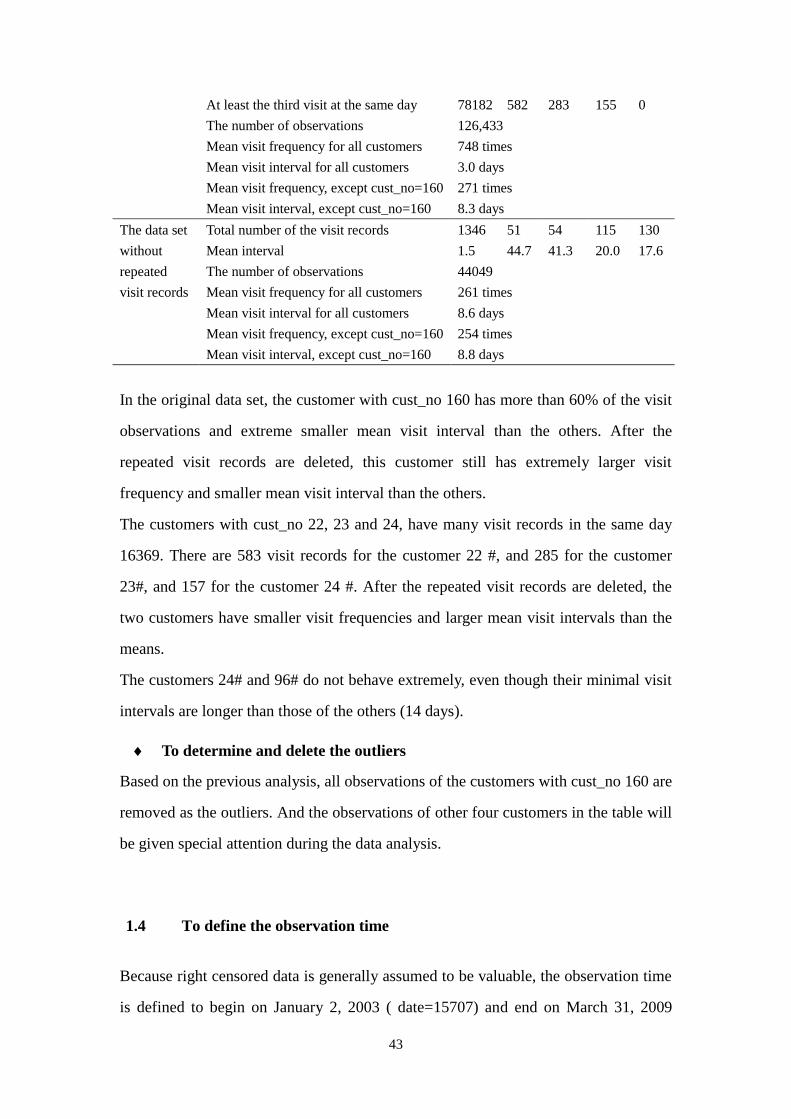
Analyzed data set

The obtained data set was referred as the analyzed data set, which included 42,454

visit intervals of 168 customers. The mean visit interval was 8.8 days, and the

standard deviation was 7 days. The minimal interval was one day and the maximal

interval was 257 days. In total 46.84% visit intervals were 7 days, and 11.98% visit

intervals were 14 days.

2.1.3 Training and Test data sets

The 42,455 observations were randomly regrouped into two subsets. Approximately

two third (27,747) of the analyzed data set were used to fit models and the rest 14,477

6

records were used to test the model performances.

2.1.4 Factors to be analyzed

Five factors were analyzed. According to the variables type and code_post in the

original data, the customers belong to four types and 92 cities. Two variables: region

and city size, were introduced and used to explore the purchase habit of customers in

11 regions and big, medium, small or tiny cities. The effect of sequence was described

by variable previous interval, which was a continuous variable from 0-42 days. For

the effect of the starting time of a purchase interval, only the effects of the 12 months

were measured according to the variable season. Considering the prediction of a new

customer, the effects of a customer (such as mean purchase interval), and the year of

observe time were not included in the study.

In the section 2.2.2, five predictors were transformed to meet the PH assumption.

2.2 Survival Analysis

Survival analysis can be performed to explore the occurrence of some events in a

population of subjects.

The time until the event is of interest, which is called the survival time or the failure

time. More often, subjects are not fully observed. The time at which a subject ceases

to be observed for some reasons other than failure is called the censoring time of the

object. All inferring about the failure time of a censored subject is that it is greater

than the censoring time. Censoring in the observed population makes survival analysis

different with other data analysis approaches.

Some regression models are developed to explore the relationship between survival

explanatory variables and predict outcomes. The Cox proportional hazards model

(Cox PH model) is one of these widely applied models.

In this study, using the PROC PHREG statement in the SAS software, a standard

7

model and a marginal model, were fitted to explore the relationship between

customer's purchase interval and five predictors. According to the results of the PH

assumption assessment, the five predictors were transformed to new covariates with

fewer subgroups, and the observe time was divided into four periods: 0-6 days, 7 days,

8-13 days, and 14+ days. The Cox PH models were piecewise fitted with the training

set and tested with the test set. The survival probabilities of the test set were

calculated based on the estimations of each model.

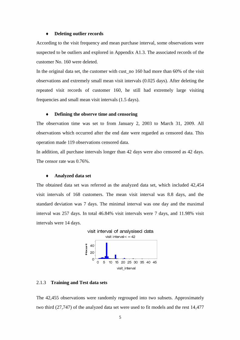
2.2.1 Theory of survival analysis

Survival and hazard probability

Two related probabilities used to describe and model the survival data are the survival

probability and the hazard probability. The survival probability S(t) is the probability

that an individual survives from the start time to a specified future time t. This term

focuses on not having an event.

)()( tTPtS (2.2.1)

The hazard is expressed as:

ttTttTPtht

/)(lim)(0

(2.2.2)

It represents the instantaneous event rate for an individual who already survived to

time t . This term describes on the occurring event.

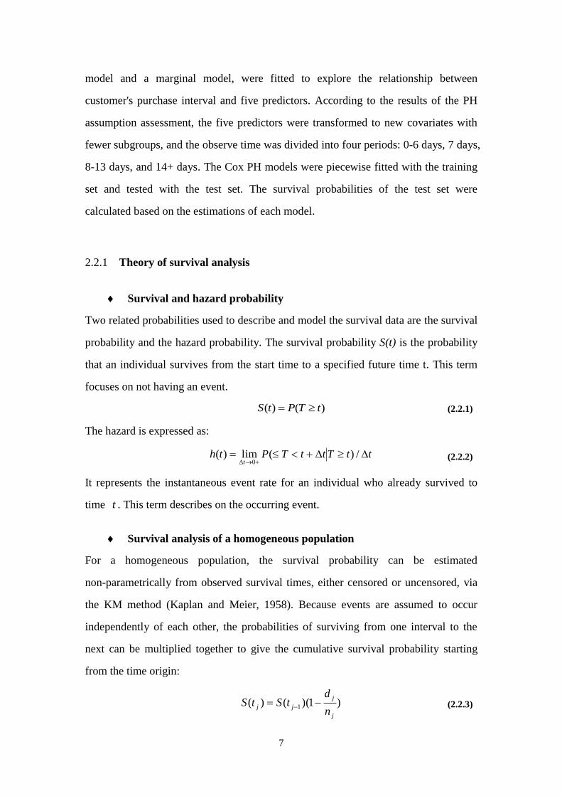
Survival analysis of a homogeneous population

For a homogeneous population, the survival probability can be estimated

non-parametrically from observed survival times, either censored or uncensored, via

the KM method (Kaplan and Meier, 1958). Because events are assumed to occur

independently of each other, the probabilities of surviving from one interval to the

next can be multiplied together to give the cumulative survival probability starting

from the time origin:

)1)(()( 1

j

j

jjn

dtStS (2.2.3)

8

For different subject groups, the survival curves can be plotted and then compared by

some nonparametric tests such as, the logrank test.

Survival analysis of an inhomogeneous population

For an inhomogeneous population, the traditional regression models, such as the

proportional hazards model, the proportional odds model, and the accelerated failure

time model (AFT model) are usually performed to measure how the properties of each

subject affect their hazard possibilities or survival times.

Usually the traditional regression models make some assumptions on the data. The

survival times are assumed to follow a specific distribution in the AFT framework,

such as the log-normal distribution, the log-logistic distribution, the generalized

gamma distribution, and the Weibull distribution. In a PH model, the hazard curves

for groups are assumed to be proportional and cannot cross.

The Cox Proportional Hazard Model

The Cox's Proportional Hazard (Cox PH) model is the most commonly employed

method in analyzing survival data. Mathematically, the basic Cox PH model is

expressed as:

)...exp()(),( 22110 ppxbxbxbthth x (2.2.4)

The hazard function ),( xth is the product of an arbitrary baseline hazard function

)(0 th with a constant term (the exponential term) which is independent with time t.

The regression parameters are estimated through the maximum partial likelihood

method without the need to know or estimate the baseline hazard function.

Proportional Hazard (PH) Assumption of Cox model

This model implies a key assumption pertaining to the data: the hazards for different

groups are proportional and the hazard ratios are constant through time.

In principle, all covariates included in a proportional hazard model must meet the PH

assumption. Thus, the assumption of proportional hazards was assessed before fitting

a Cox PH model. Usually, the proportional hazard assumption can be checked by

9

three types of methods: the graphical methods or using an extended Cox model or

using a goodness of fit test.

In practice, PH is assumed to hold unless there is very strong evidence to counter this

assumption such as, 1) estimated survival curves are fairly separated, then cross, 2)

estimated survival curves look very unparallel over time, 3) weighted Schoenfeld

residuals clearly increase or decrease over time, 4) a test for interaction term between

time and covariates is significant (r.f. time dependent covariates).

Violation of PH Assumption and extended Cox PH model

When the PH assumption does hold, the related covariate can be transformed to meet

with the PH assumption. If the effect of the covariate does not need to be estimated, a

stratified Cox PH model can be fitted. In some case, a extended Cox PH model

incorporates with time-dependent covariates allows the hazard ratio to fluctuate and

relaxes the proportionality assumption to some extent.

))(exp()())(,( 0 tthtth bxx (2.2.5)

Recurrent events and marginal Cox PH model

Some events of a given subject may occur more than once over the follow-up time .

Such events are called recurrent events. A widely used technique for adjusting the

correlation among recurrent events of a subject is the robust estimation method.

Several different approach employ this technique have been suggested to build a Cox

PH model from survival data with recurrent events (M. Gail, 2005). The major

differences in these approaches lie in the way how the start time and the end time of

an interval are defined, and weather a strata model is fitted or not.

Goodness of fit: graphical methods

Both graphical methods and test approaches are available for assessing the goodness

of fit in fitting a proportional hazards model.

Graphical methods are based on residuals. Five kinds of residuals are defined for

censored survival data, namely the Cox-Snell residual, the martingale residual, the

martingale residual, the Schoenfeld residual, and the weighted Schoenfeld residual.

10

The Cox-Snell residual is not so desirable for a proportional hazards model, where a

partial likelihood function is used and the survivorship function is estimated by

nonparametric methods (Elisa T. Lee, 2003). The martingale residuals have a skewed

distribution with mean zero. The deviance residuals also have a mean of zero but are

symmetrically distributed about zero when the fitted model is adequate. Deviance

residuals are positive for persons who survive for a shorter time than expected and

negative for those who survive longer. The weighted Schoenfeld residuals have better

diagnostic power than the un-weighted residuals in assessing the proportional hazards

assumption.

Usually, the deviance and weighted Schoenfeld residuals against the survival time or

a covariate are plotted to check the adequacy of a proportional hazards model. The

presence of certain patterns in these graphs may indicate departures from the

proportional hazards assumption, while extreme departures from the main cluster

indicate possible outliers or potential stability problems of the model.

Goodness of fit: testing approach

The testing approach is a variant of the Schoenfeld residuals versus survival time plot.

Once a Cox PH model was fitted, the Schoenfeld residuals for each predictor can be

calculated. A new variable is used to rank the order of failures. The subject with the

earliest event is assigned a value of 1, the next 2, and so on. The null hypothesis is

that the correlation between the Schoenfeld residuals and the ranked failure time is

zero. Rejecting the null hypothesis indicates that the PH assumption is violated.

For the test approach, a p-value can be driven by the sample size. A gross violation of

the null assumption may not be statistically significant if the sample size is too small.

Conversely, a slight violation of the null assumption may be highly significant if the

sample size is sufficiently large (M. Gail, 2005).

2.2.2 Covariates and their PH Assumption Assessment

Five factors described in the section 2.1.4were studied. Continuous variable previous

interval was categorized to many groups. The variable type, region, season, and size

11

have 4, 11, 12, and 4 groups.

Plots of ))](ˆlog(log[ tS versus log (t) for subgroups of five factors were employed

to evaluate the proportional hazard assumption. )(ˆ tS was estimated by the KM

method (Kaplan and Meier). If the PH model is appropriate for a given predictor, it

can be expected that empirical plots of log-log survival curves for different subgroups

are approximately parallel.

For each of the other four categorical variables, the subgroups were combined until

the curves were parallel. After the combination, 42454 observations of 168 customers

belong to three previous interval groups, four customer types, four regions, four

seasons and two city sizes. The frequencies of subgroups of five covariates are listed

in table 2.2.1. The details on how the subgroups of each factors are chosen can be

found in the Appendix A-2.

Table 2.2.1 Frequency table of five covariates

Covariates Subgroups & Frequency Sum

Previous 0-6 days 7-13 days 14+ days /

interval 9454 24997 8003 42454

City size Tiny &

Small

Medium

& Big

/ /

108 60 168 customers

27034 15420 42454

Season Apr.~Jun. Jul.~Aug. Sep.~Nov.,

Jan.~Mar.

Dec.

11479 7832 19833 3292

Type Horeca Catering Particulier Retail

82 71 8 7 168 customers

18155 20574 1742 1983 42454

Region Vlaams

Braban

Waals

Brabant

West V.,

Limburg,

Luxembourg

Other

provinces

10 1 61 96 168 customers

2535 237 16514 23168 42454

As shown in Figure 2.2.1, after combination, the KM estimated survival curves of the

subgroups may crossed at 7th

day, 8th

days and 14th

day, but are piecewise parallel

within three time spans: 0-6 days, 8-13 days, and 14+ days. The curves can be

12

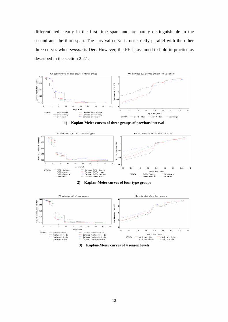
differentiated clearly in the first time span, and are barely distinguishable in the

second and the third span. The survival curve is not strictly parallel with the other

three curves when season is Dec. However, the PH is assumed to hold in practice as

described in the section 2.2.1.

1) Kaplan-Meier curves of three groups of previous interval

2) Kaplan-Meier curves of four type groups

3) Kaplan-Meier curves of 4 season levels

13

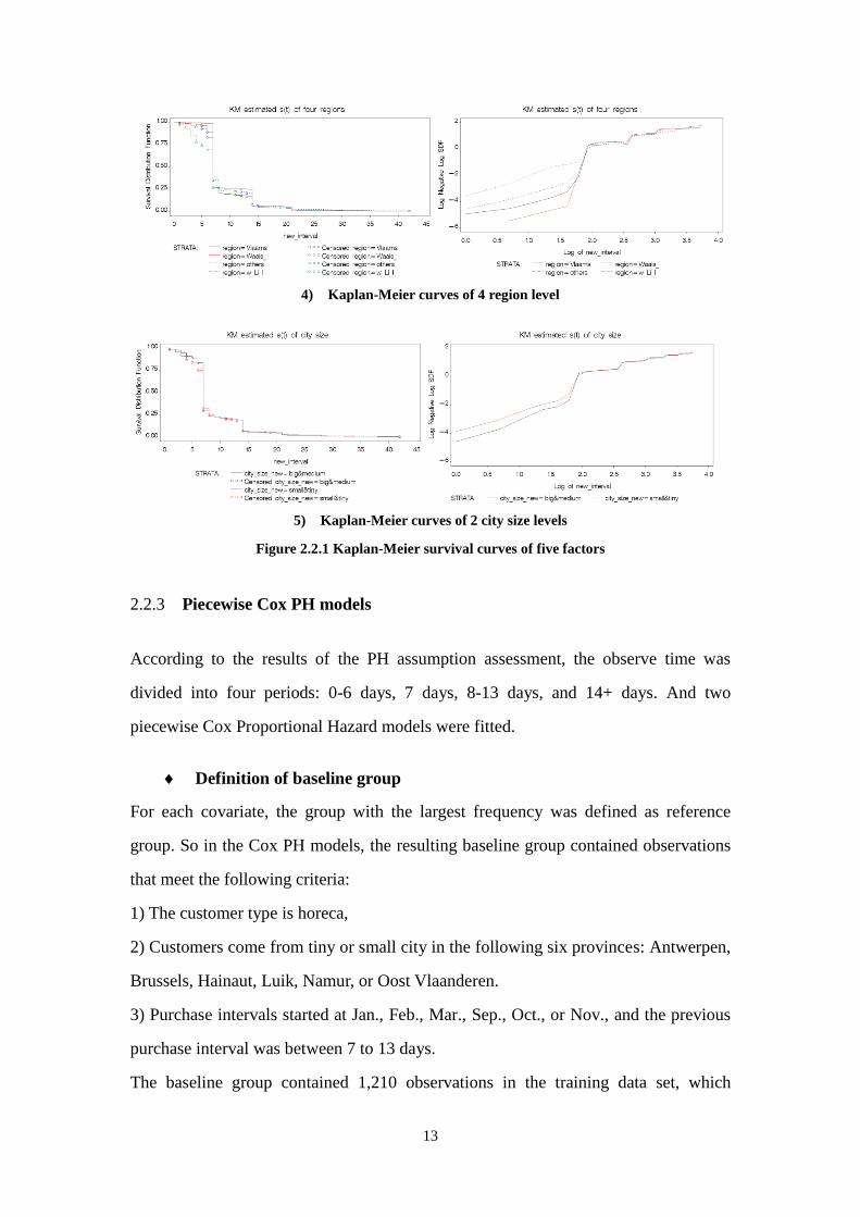
4) Kaplan-Meier curves of 4 region level

5) Kaplan-Meier curves of 2 city size levels

Figure 2.2.1 Kaplan-Meier survival curves of five factors

2.2.3 Piecewise Cox PH models

According to the results of the PH assumption assessment, the observe time was

divided into four periods: 0-6 days, 7 days, 8-13 days, and 14+ days. And two

piecewise Cox Proportional Hazard models were fitted.

Definition of baseline group

For each covariate, the group with the largest frequency was defined as reference

group. So in the Cox PH models, the resulting baseline group contained observations

that meet the following criteria:

1) The customer type is horeca,

2) Customers come from tiny or small city in the following six provinces: Antwerpen,

Brussels, Hainaut, Luik, Namur, or Oost Vlaanderen.

3) Purchase intervals started at Jan., Feb., Mar., Sep., Oct., or Nov., and the previous

purchase interval was between 7 to 13 days.

The baseline group contained 1,210 observations in the training data set, which

14

contained 27,747 observations.

Standard Cox PH model

First, we assumed that the observations of a customer were independent with each

other, and the censored observations were non informative censor. A standard Cox

model was fitted for the training set. Within each of four time spans, five covariates

and their two-ordered interactions were measured. The AIC value was employed to

choose the final model.

Marginal Cox PH model

Second, the following SAS code was used to fit a marginal model with the training

set.

PROC PHREG DATA=taining_set COVS(AGGREGATE);

MODEL (date1, date4)*censor(1)= list of covariates and interactions ;

ID cust_no; RUN;

This code follows the counting processing approach recommended by M. Gail et al.

(M. Gail, 2005). The COVS(AGGREGATE) option in the PROC PHREG statement

requires robust standard errors of the parameter estimates. The time intervals for each

observation are defined by the variables date1 and date4. For each customer, the first

visit interval starts from 0 day. The variable cust_no is used as the ID in this proc

statement.

The covariates and interactions measured in the marginal model were the same as

those in the standard model. The censored observations were assumed to be non

informative censor. The variances of the estimated regression coefficients were

adjusted to handle the correlation among the observations of a custom. But this model

did not account for the occurrence order of recurrent events. If a STRATA statement

was used (STRATA interval; variable interval= date4-date1 ), the order in which

recurrent events occur will be accounted for.

2.2.4 Prediction of survival probabilities of the test set

Usually, the BASELINE statement in PROC PHREG can be employed to output the

15

Kalbfleisch/Prentice estimator of the baseline hazard, and estimates of survival at

arbitrary values of the covariates.

However, since piecewise Cox PH models were fitted in this study, the BASELINE

statement did not work. The prediction of survival probabilities for the test set was

performed according to equations (2.2.6~2.2.10). The baseline survival functions

were approximated by KM survival estimators of the baseline group in the training

set.

)exp()]})( Slog([)])( Slog({[

)exp()]})( Slog([)])( Slog({[

)exp()]})( Slog([)])( Slog({[

)exp()])( Slog([

)exp()](H)(H[

)exp()](H)(H[

)exp()](H)(H[

)exp()(H

)exp()(h)exp()(h

)exp()(h)exp()(h

),(h),(h),(h),(h),(H

3300

22030

11020

10

3300

22030

11020

10

3

3

02

3

2

0

1

2

1

0

1

0

0

3

3

2

2

1

1

0

xb

xb

xb

bx

xb

xb

xb

bx

xbxb

xbbx

xxxxx

tt

tt

tt

t

tt

tt

tt

t

duuduu

duuduu

duuduuduuduut

t

t

t

t

t

t

t

t

t

t

t

t

t

t

(2.2.6)

)exp(

0

)exp()exp(

30

)exp()exp(

20

)exp()exp(

10

)exp(

300

)exp(

2030

)exp(

1020

)exp(

10

)exp(

300

)exp(

2030

)exp(

1020

)exp(

10

3300

2030

1020

10

3

33

3

3

])( S[])( S[

])( S[])( S[

])( )/S( S[])( )/S( S[

])( )/S( S[])( S[

)]})( Slog())( S{exp[log(

)]})( Slog())( S{exp[log(

)]})( Slog())( S{exp[log(

]})( S{exp[log(

)}exp()])( Slog())( S[log(

)}exp()])( Slog())( S[log(

)exp()])( Slog())( S[log(

)exp())( Sexp{log(

)(for)),(Hexp(),(S

xbxbxb

xbxbxbbx

xbxb

xbbx

xb

xb

xb

bx

2

1

2

211

2

1

2

1

xb

xb

xb

bx

xx

tt

tt

tttt

ttt

tt

tt

tt

t

tt

tt

tt

t

tttt

(2.2.7)

)for(])( S[*])( S[*])( S[

)),(Hexp(),(S

23

)exp(

0

)exp()exp(

20

)exp()exp(

10 tttttt

tt

xβxβxβxββx 2211

xx (2.2.8)

16

)for(])( S[*])( S[),(S 12

)exp(

0

)exp()exp(

10 tttttt xβxββx 11x (2.2.9)

)for(])( S[),(S 1

)exp(

0 tttt βxx (2.2.10)

2.3 Neural network survival analysis

As mentioned in Chapter 1, the assumptions of the traditional regression models may

be untenable in some situations and modeling the underlying relationships of

multivariate data implies a definition of a correct functional relationship among the

considered variables.

To address these problems, ANN approaches can be employed to perform predictions

of the survival times, survival and hazard.

2.3.1 Theory of neural network survival analysis

Three kinds of methods have been suggested to employ the neural network method in

survival analysis.

1) Direct prediction of survival time

The neural network survival analysis has been employed to predict the survival time

of a subject directly from the given inputs (C. J. S. deSilva, 1994) (P. L. Choong,

1993). However, few applications were developed further.

2) As an extension to a Cox PH model

Faraggi and Simon (Faraggi, 1995) used the ANN predictor as an extension to the

linear proportional hazard Cox model. The authors suggested fitting a neural network

with a single logistic hidden layer and a linear output layer and replacing the linear

predictor in the Cox PH model with the non-linear output of the network.

L. Mariani et al. (L. Mariani, 1997) used both the standard Cox model and the

neural network method recommended by Faraggi and Simonto assess the prognostic

factors for the recurrence of the breast cancer. The authors stated that the results from

17

the ANN approach were substantially overlapped with those from the standard Cox

model in the pattern of the effect of prognostic variables and predictive values. The

ANN approach showed the potential to outperform conventional regression

techniques when complex interactions or non-linear effects of continuous predictors

existed.

However, these extensions were still regarded as a sub-optimal way to model the

baseline variation, although this method allowed preserving all the advantages of a

classical proportional hazards model (Bart Baesens, 2005).

3) Prediction of probabilities

Some other studies set the survival status of a subject as the target of the neural

network. Different data structures, network structures and network activation

functions were proposed by Liestol et al. (1994), Stephen F. Brown et al. (1997),

Ravdin, P. M. et al.(1992), and Elia Biganzolil et al (1998) . The outputs of networks

were proved to be the survival or hazard probability.

Some of these approaches have an output layer with one output node and permit time

dependent covariates. The data set need to be transforms before training the network.

Usually the size of the transformed data set networks is as large as several times of the

size of the data set without transforming, and the training the network is time

consuming.

The other approaches permit many output nodes in an output layer. The size of

transformed data set does not increase, while the structure of the network does not

support time dependent covariates.

This method is applied by most of studies which employed ANN to analysis survival

data. However, few studies compare the prediction abilities of these approaches.

An example with two observations shown in table 2.3.1 illustrates those modification

strategies on the data structures. The case includes two covariates X1 and X2. The

subject A was censored on the third day, and the subject B fails on the fourth day. The

total follow-up time is 5 days.

18

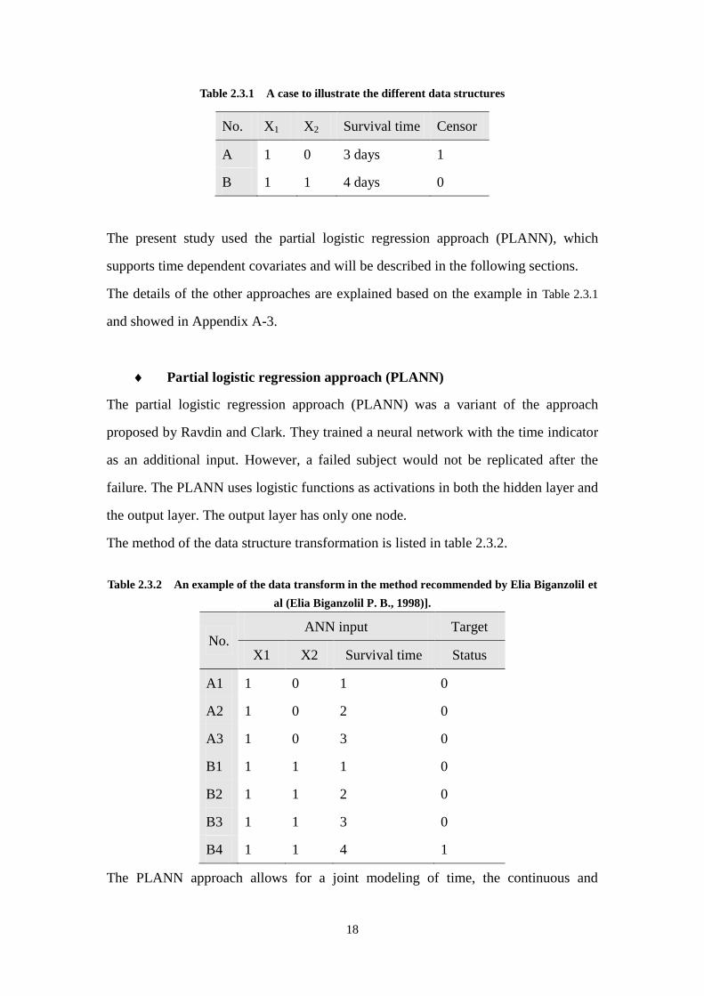
Table 2.3.1 A case to illustrate the different data structures

No. X1 X2 Survival time Censor

A 1 0 3 days 1

B 1 1 4 days 0

The present study used the partial logistic regression approach (PLANN), which

supports time dependent covariates and will be described in the following sections.

The details of the other approaches are explained based on the example in Table 2.3.1

and showed in Appendix A-3.

Partial logistic regression approach (PLANN)

The partial logistic regression approach (PLANN) was a variant of the approach

proposed by Ravdin and Clark. They trained a neural network with the time indicator

as an additional input. However, a failed subject would not be replicated after the

failure. The PLANN uses logistic functions as activations in both the hidden layer and

the output layer. The output layer has only one node.

The method of the data structure transformation is listed in table 2.3.2.

Table 2.3.2 An example of the data transform in the method recommended by Elia Biganzolil et

al (Elia Biganzolil P. B., 1998)].

No. ANN input Target

X1 X2 Survival time Status

A1 1 0 1 0

A2 1 0 2 0

A3 1 0 3 0

B1 1 1 1 0

B2 1 1 2 0

B3 1 1 3 0

B4 1 1 4 1

The PLANN approach allows for a joint modeling of time, the continuous and

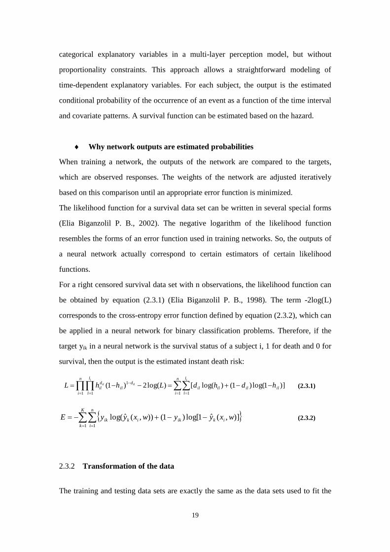
19

categorical explanatory variables in a multi-layer perception model, but without

proportionality constraints. This approach allows a straightforward modeling of

time-dependent explanatory variables. For each subject, the output is the estimated

conditional probability of the occurrence of an event as a function of the time interval

and covariate patterns. A survival function can be estimated based on the hazard.

Why network outputs are estimated probabilities

When training a network, the outputs of the network are compared to the targets,

which are observed responses. The weights of the network are adjusted iteratively

based on this comparison until an appropriate error function is minimized.

The likelihood function for a survival data set can be written in several special forms

(Elia Biganzolil P. B., 2002). The negative logarithm of the likelihood function

resembles the forms of an error function used in training networks. So, the outputs of

a neural network actually correspond to certain estimators of certain likelihood

functions.

For a right censored survival data set with n observations, the likelihood function can

be obtained by equation (2.3.1) (Elia Biganzolil P. B., 1998). The term -2log(L)

corresponds to the cross-entropy error function defined by equation (2.3.2), which can

be applied in a neural network for binary classification problems. Therefore, if the

target yik in a neural network is the survival status of a subject i, 1 for death and 0 for

survival, then the output is the estimated instant death risk:

)]1log()1()log([)log(2)1(1 11 1

1

ililil

n

i

l

l

il

n

i

l

l

d

il

d

il hdhdLhhLii

ilil

(2.3.1)

K

k

n

i

ikikikik wxyywxyyE1 1

)],(ˆ1log[)1()),(ˆlog( (2.3.2)

2.3.2 Transformation of the data

The training and testing data sets are exactly the same as the data sets used to fit the

20

Cox PH models. The data sets were first transformed in order to fit a neural

networking model, as described in Section 2.3.1. An example is shown to illustrate

the transformation in table 2.3.3 and table 2.3.4. Table 2.3.3 contains the two original

observations, and the transformed observations are listed in table 2.3.4

Table 2.3.3 The original observations

Previous

interval

type Season region City size Purchase

interval

Censor

0-6 days Catering Dec. Waals B Medium 2 1

7-13 days Horeca Jul. Luik Tiny 3 0

Table 2.3.4 The transformed observations:

Previous

interval

type season region City size Survival

time

Survival

status

0-6 days Catering Dec. Waals B Medium 1 0

0-6 days Catering Dec. Waals B Medium 2 0

7-13 days Horeca Jul. Luik Tiny 1 0

7-13 days Horeca Jul. Luik Tiny 2 0

7-13 days Horeca Jul. Luik Tiny 3 1

2.3.3 ANN Model

In this study, the function nnet( ) in the R software package was employed to train a

Partial Logistic Artificial Neural Network (PLANN) (Elia Biganzolil P. B., 1998).

This network contains one input layer with six nodes, one hidden layer with seven

nodes, and one output node. The training and testing data sets are exactly the same as

the data sets used to fit the Cox PH models.

Input, target and output

The input layer of the PLANN model had six neurons. Five of them were predictors,

which were the same as the predictors in Cox PH models; the last one was a time

indicator, which was the survival time.

A binary target，the survival status had a value of either 0 or 1. The single output

neuron provided the conditional probability of a consequent purchase.

Model optimization

21

Several techniques were used to improve the prediction ability. A penalty term

2

kjw , usually called the weight decay, was added to the error function. The

error function was further regularized by setting maximum number of iterations to

1,000 in the back-propagation (maxit=1000 in nnet()).

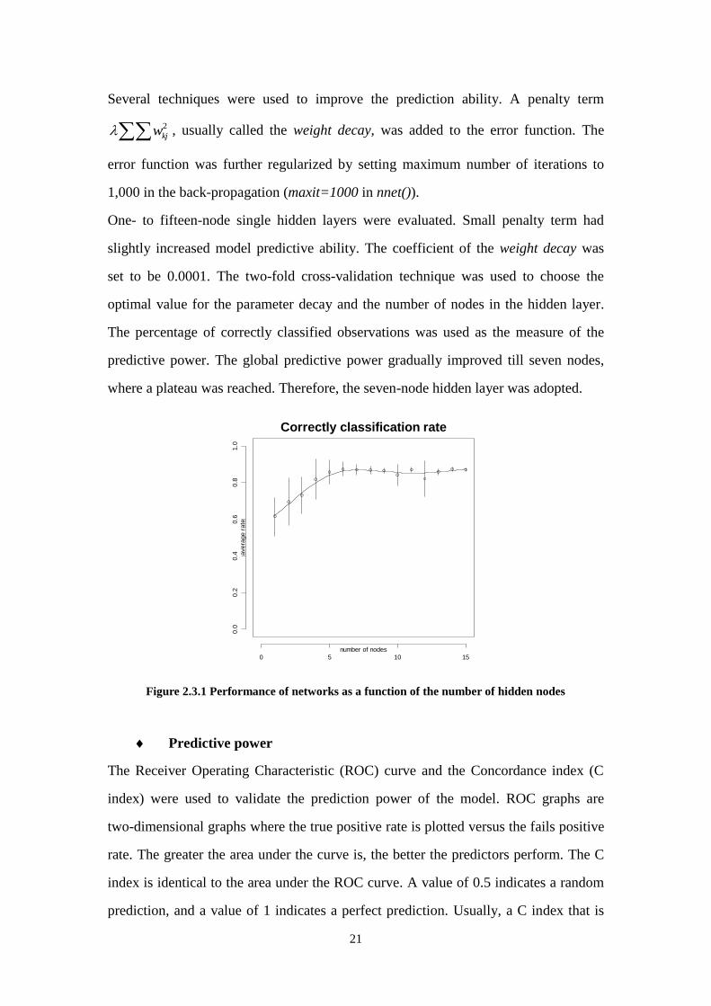
One- to fifteen-node single hidden layers were evaluated. Small penalty term had

slightly increased model predictive ability. The coefficient of the weight decay was

set to be 0.0001. The two-fold cross-validation technique was used to choose the

optimal value for the parameter decay and the number of nodes in the hidden layer.

The percentage of correctly classified observations was used as the measure of the

predictive power. The global predictive power gradually improved till seven nodes,

where a plateau was reached. Therefore, the seven-node hidden layer was adopted.

Figure 2.3.1 Performance of networks as a function of the number of hidden nodes

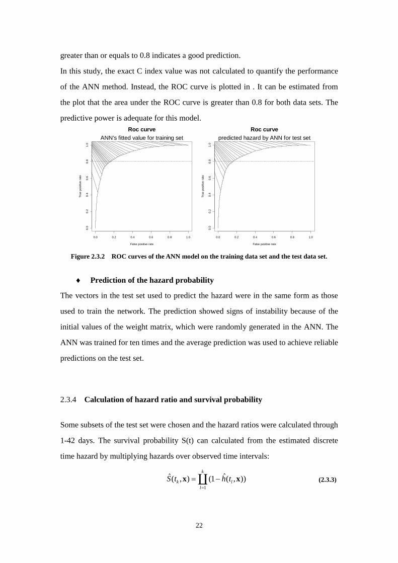
Predictive power

The Receiver Operating Characteristic (ROC) curve and the Concordance index (C

index) were used to validate the prediction power of the model. ROC graphs are

two-dimensional graphs where the true positive rate is plotted versus the fails positive

rate. The greater the area under the curve is, the better the predictors perform. The C

index is identical to the area under the ROC curve. A value of 0.5 indicates a random

prediction, and a value of 1 indicates a perfect prediction. Usually, a C index that is

0 5 10 15

0.0

0.2

0.4

0.6

0.8

1.0

Correctly classification rate

number of nodes

avera

ge r

ate

22

greater than or equals to 0.8 indicates a good prediction.

In this study, the exact C index value was not calculated to quantify the performance

of the ANN method. Instead, the ROC curve is plotted in . It can be estimated from

the plot that the area under the ROC curve is greater than 0.8 for both data sets. The

predictive power is adequate for this model.

Figure 2.3.2 ROC curves of the ANN model on the training data set and the test data set.

Prediction of the hazard probability

The vectors in the test set used to predict the hazard were in the same form as those

used to train the network. The prediction showed signs of instability because of the

initial values of the weight matrix, which were randomly generated in the ANN. The

ANN was trained for ten times and the average prediction was used to achieve reliable

predictions on the test set.

2.3.4 Calculation of hazard ratio and survival probability

Some subsets of the test set were chosen and the hazard ratios were calculated through

1-42 days. The survival probability S(t) can calculated from the estimated discrete

time hazard by multiplying hazards over observed time intervals:

k

l

lk thtS1

)),(ˆ1(),(ˆ

xx (2.3.3)

False positive rate

Tru

e p

ositiv

e r

ate

0.0 0.2 0.4 0.6 0.8 1.0

0.0

0.2

0.4

0.6

0.8

1.0

Roc curve

ANN's fitted value for training set

False positive rate

Tru

e p

ositiv

e r

ate

0.0 0.2 0.4 0.6 0.8 1.0

0.0

0.2

0.4

0.6

0.8

1.0

Roc curve

predicted hazard by ANN for test set

23

2.4 Comparison

2.4.1 Subgroups to be compared

In this study, in total 13 subsets of the test set were selected and the hazard ratios

between subsets were then calculated.

One of subsets was defined as the reference group. This group contained observations

that met the following criteria: 1) the customer type is horeca, 2) customers come

from tiny or small city of following six provinces: Antwerpen, Brussels, Hainaut,

Luik, Namur, or Oost Vlaanderen. 3) Purchase intervals started at Jan., Feb., Mar.,

Sep.,Oct., or Nov., and the previous purchase interval was between 7 to 13 days.

Compared to the reference group, each of the rest subsets had only one covariate

changed respectively: 1) previous interval <7days, 2) previous interval > 13 days, 3)

type=catering, 4) type=particulier, 5) type=retail, 6) city size= big & medium, 7)

region= West Vlaaderen, Limburg, or Luxembourg, 8) region =Vlaams Braban, 9)

region=Waals Brabant, 10) season=Apr.-Jun., 11) season= Jul.-Aug., 12)

season=Dec..

2.4.2 Comparison of hazard ratios and survival probabilities

The hazard ratios of 12 subgroups to the reference groups were calculated based on

the outputs of the two Cox PH models and the ANN model. For the ANN model, the

observation time of the reference group was 1-34 days. The hazard ratios were

calculated through 1-34 days and clustered separately in four time spans: 0-6 days, 7

days, 8-13 days and 14-34 days. The estimated hazard ratios reflected relative effects

of five factors on the purchase behavior of a customer.

For some of the subgroups, four survival curves were plotted: 1) the curves generated

directly from the test set (Kaplan Meier). 2), 3) the curves predicted by two Cox PH

models and 4) the curves predicted by the neural network. The survival curves were

then compared to each other according to their confidence intervals. The comparisons

reflected the prediction abilities of the three models.

24

3 Results

3.1 Hazard ratios

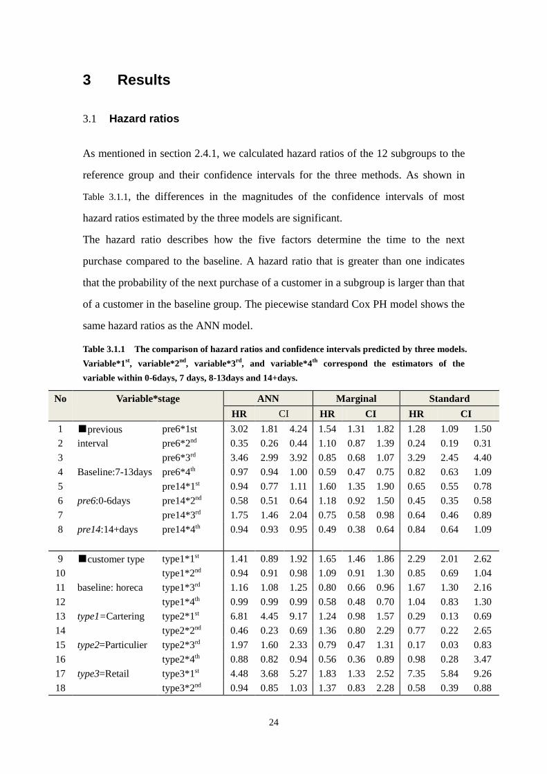
As mentioned in section 2.4.1, we calculated hazard ratios of the 12 subgroups to the

reference group and their confidence intervals for the three methods. As shown in

Table 3.1.1, the differences in the magnitudes of the confidence intervals of most

hazard ratios estimated by the three models are significant.

The hazard ratio describes how the five factors determine the time to the next

purchase compared to the baseline. A hazard ratio that is greater than one indicates

that the probability of the next purchase of a customer in a subgroup is larger than that

of a customer in the baseline group. The piecewise standard Cox PH model shows the

same hazard ratios as the ANN model.

Table 3.1.1 The comparison of hazard ratios and confidence intervals predicted by three models.

Variable*1st, variable*2

nd, variable*3

rd, and variable*4

th correspond the estimators of the

variable within 0-6days, 7 days, 8-13days and 14+days.

No Variable*stage ANN Marginal Standard

HR CI HR CI HR CI

1 ■previous

interval

Baseline:7-13days

pre6:0-6days

pre14:14+days

pre6*1st 3.02 1.81 4.24 1.54 1.31 1.82 1.28 1.09 1.50

2 pre6*2nd 0.35 0.26 0.44 1.10 0.87 1.39 0.24 0.19 0.31

3 pre6*3rd 3.46 2.99 3.92 0.85 0.68 1.07 3.29 2.45 4.40

4 pre6*4th 0.97 0.94 1.00 0.59 0.47 0.75 0.82 0.63 1.09

5 pre14*1st 0.94 0.77 1.11 1.60 1.35 1.90 0.65 0.55 0.78

6 pre14*2nd 0.58 0.51 0.64 1.18 0.92 1.50 0.45 0.35 0.58

7 pre14*3rd 1.75 1.46 2.04 0.75 0.58 0.98 0.64 0.46 0.89

8 pre14*4th 0.94 0.93 0.95 0.49 0.38 0.64 0.84 0.64 1.09

9 ■customer type

baseline: horeca

type1=Cartering

type2=Particulier

type3=Retail

type1*1st 1.41 0.89 1.92 1.65 1.46 1.86 2.29 2.01 2.62

10 type1*2nd 0.94 0.91 0.98 1.09 0.91 1.30 0.85 0.69 1.04

11 type1*3rd 1.16 1.08 1.25 0.80 0.66 0.96 1.67 1.30 2.16

12 type1*4th 0.99 0.99 0.99 0.58 0.48 0.70 1.04 0.83 1.30

13 type2*1st 6.81 4.45 9.17 1.24 0.98 1.57 0.29 0.13 0.69

14 type2*2nd 0.46 0.23 0.69 1.36 0.80 2.29 0.77 0.22 2.65

15 type2*3rd 1.97 1.60 2.33 0.79 0.47 1.31 0.17 0.03 0.83

16 type2*4th 0.88 0.82 0.94 0.56 0.36 0.89 0.98 0.28 3.47

17 type3*1st 4.48 3.68 5.27 1.83 1.33 2.52 7.35 5.84 9.26

18 type3*2nd 0.94 0.85 1.03 1.37 0.83 2.28 0.58 0.39 0.88

25

19 type3*3rd 1.47 1.31 1.63 0.80 0.49 1.31 1.67 0.94 2.98

20 type3*4th 0.98 0.96 1.00 0.49 0.29 0.83 0.69 0.42 1.13

21 ■citysize

baseline:

tiny&small

City_size

=big&medium,

city_size*1st 1.08 0.94 1.22 1.44 1.25 1.65 1.21 1.07 1.37

22 city_size*2nd 1.01 0.96 1.06 1.13 0.92 1.37 0.92 0.77 1.11

23 city_size*3rd 1.01 1.00 1.03 0.93 0.74 1.17 1.17 0.92 1.49

24 city_size*4th 1.03 1.01 1.05 0.61 0.49 0.76 1.13 0.91 1.41

25 ■region

baseline: others

region1=West

Vlaanderen,

Limburg, or

Luxembourg,

region2=VlaamsB

region3=WaalsB

region1*1st 2.70 1.44 3.95 1.81 1.55 2.11 1.53 1.36 1.73

26 region1*2nd 0.98 0.90 1.06 1.12 0.90 1.38 0.93 0.77 1.11

27 region1*3rd 1.25 1.07 1.42 0.86 0.68 1.08 0.84 0.66 1.06

28 region1*4th 0.96 0.95 0.98 0.46 0.36 0.58 0.68 0.55 0.84

29 region2*1st 0.87 0.82 0.93 1.44 1.02 2.04 0.98 0.63 1.52

30 region2*2nd 1.06 1.02 1.11 1.38 0.87 2.18 0.93 0.49 1.77

31 region2*3rd 1.05 0.99 1.11 0.98 0.55 1.73 0.52 0.22 1.22

32 region2*4th 0.98 0.98 0.98 0.55 0.33 0.91 0.94 0.48 1.88

33 region3*1st 0.60 0.44 0.77 4.51 2.77 7.33 0.07 0.01 0.48

34 region3*2nd 1.07 1.03 1.12 1.49 0.74 2.98 1.26 0.08 20.55

35 region3*3rd 1.04 0.96 1.12 0.53 0.21 1.31 0.45 0.02 9.13

36 Region3*4th 0.98 / / 0.60 0.29 1.24 1.74 0.10 29.29

37 ■season

baseline: others

m4_6=Apr.-Jun.,

m7_8=Jul.-Aug.,

m12=Dec..

m4_6*1st 1.10 0.97 1.23 1.64 1.44 1.86 1.42 1.27 1.59

38 m4_6*2nd 0.86 0.82 0.91 1.24 1.03 1.49 1.23 1.04 1.46

39 m4_6*3rd 0.88 0.81 0.95 0.79 0.65 0.97 1.59 1.27 2.01

40 m4_6*4th 0.92 0.91 0.94 0.60 0.49 0.74 1.15 0.95 1.40

41 m7_8*1st 1.34 1.30 1.37 1.66 1.46 1.90 1.58 1.40 1.80

42 m7_8*2nd 1.08 1.03 1.12 1.24 1.04 1.49 1.10 0.91 1.33

43 m7_8*3rd 1.25 1.20 1.29 0.82 0.66 1.00 1.35 1.03 1.76

44 m7_8*4th 1.09 1.07 1.12 0.49 0.40 0.60 0.68 0.54 0.84

45 m12*1st 1.78 1.41 2.15 1.60 1.32 1.94 0.71 0.56 0.88

46 m12*2nd 1.04 0.99 1.09 1.26 0.97 1.65 0.69 0.49 0.97

47 m12*3rd 1.09 0.97 1.21 0.79 0.60 1.05 0.78 0.52 1.17

48 m12*4th 0.97 0.94 0.99 0.50 0.38 0.67 0.60 0.43 0.84

3.2 Factor effects

The survival probabilities of the test set were predicted or calculated by the three

models for five factors: previous interval, customer type, city size, region and season.

The effects of each of factors are evaluated by maintaining the other four factors the

same as those of the reference group and calculating the cumulative hazards and the

26

survivals.

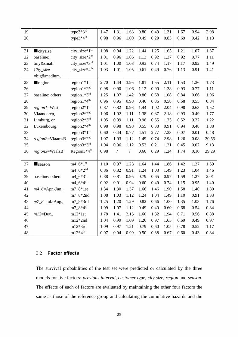
The comparison results of the factor city size are displayed in Figure 3.2.1. The upper

part displays the estimated cumulative hazard plot and the bottom part displays the

survival curves.

Figure 3.2.1 Comparison of survival functions and cumulative hazards among different city size

The comparison results of the other four factors, the seasons, the previous interval,

the customer type, and the regions are displayed in Figure 3.2.2, Figure 3.2.3, Figure

3.2.4 and Figure 3.2.5, respectively in a similar way.

27

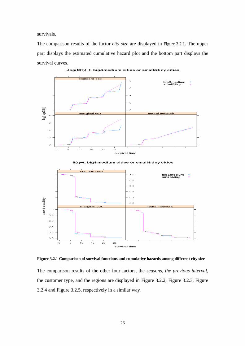
Figure 3.2.2 Comparison of survival functions and cumulative hazards among different season

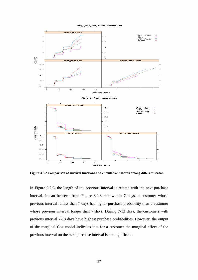
In Figure 3.2.3, the length of the previous interval is related with the next purchase

interval. It can be seen from Figure 3.2.3 that within 7 days, a customer whose

previous interval is less than 7 days has higher purchase probability than a customer

whose previous interval longer than 7 days. During 7-13 days, the customers with

previous interval 7-13 days have highest purchase probabilities. However, the output

of the marginal Cox model indicates that for a customer the marginal effect of the

previous interval on the next purchase interval is not significant.

28

Figure 3.2.3 Comparison of survival functions and cumulative hazards among different season

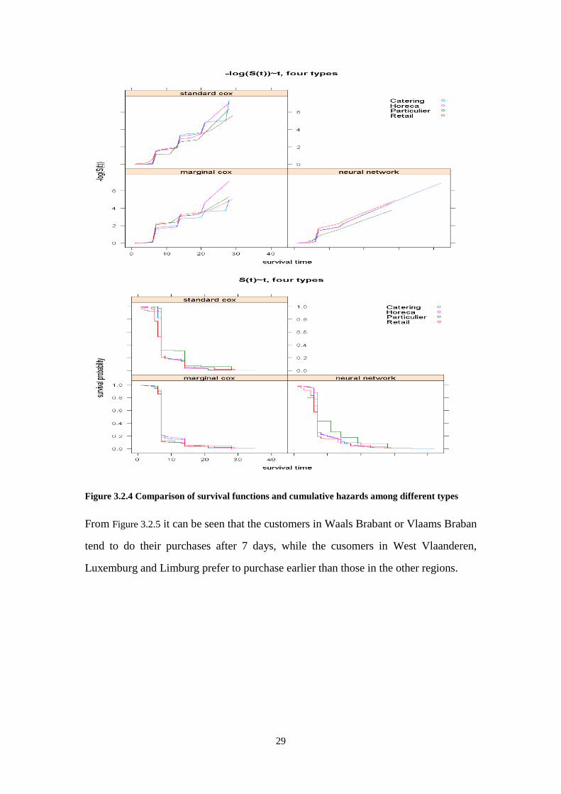
As shown in Figure 3.2.4, the customers whose types are ‘catering’ or ‘horeca’ have

similar purchase trends and have shorter purchase intervals than that of other type

customers. The ‘particulier’ customers tend to do their next purchase later. For a

‘retail’ customer, the standard Cox model and ANN model give different results.

29

Figure 3.2.4 Comparison of survival functions and cumulative hazards among different types

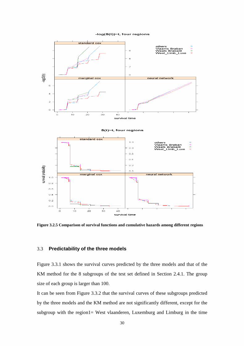
From Figure 3.2.5 it can be seen that the customers in Waals Brabant or Vlaams Braban

tend to do their purchases after 7 days, while the cusomers in West Vlaanderen,

Luxemburg and Limburg prefer to purchase earlier than those in the other regions.

30

Figure 3.2.5 Comparison of survival functions and cumulative hazards among different regions

3.3 Predictability of the three models

Figure 3.3.1 shows the survival curves predicted by the three models and that of the

KM method for the 8 subgroups of the test set defined in Section 2.4.1. The group

size of each group is larger than 100.

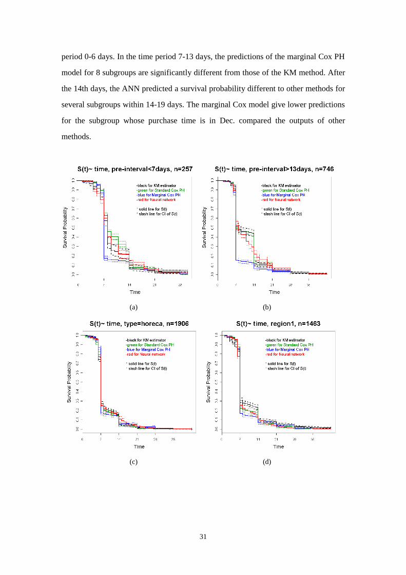
It can be seen from Figure 3.3.2 that the survival curves of these subgroups predicted

by the three models and the KM method are not significantly different, except for the

subgroup with the region1= West vlaanderen, Luxemburg and Limburg in the time

31

period 0-6 days. In the time period 7-13 days, the predictions of the marginal Cox PH

model for 8 subgroups are significantly different from those of the KM method. After

the 14th days, the ANN predicted a survival probability different to other methods for

several subgroups within 14-19 days. The marginal Cox model give lower predictions

for the subgroup whose purchase time is in Dec. compared the outputs of other

methods.

(a) (b)

(c) (d)

32

(e) (f)

(g) (h)

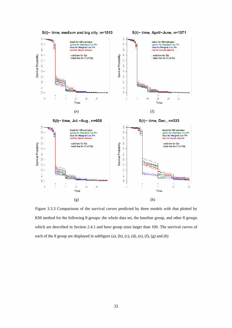
Figure 3.3.3 Comparisons of the survival curves predicted by three models with that plotted by

KM method for the following 8 groups: the whole data set, the baseline group, and other 8 groups

which are described in Section 2.4.1 and have group sizes larger than 100. The survival curves of

each of the 8 group are displayed in subfigure (a), (b), (c), (d), (e), (f), (g) and (h)

33

4 Discussion and Conclusion

4.1 Conclusion

Compared to the KM method estimators, the performance of the ANN is bad for the

subgroup with previous interval longer than 13 days. And the predictions of the

standard Cox PH model for the subgroup with previous interval less than 7 days are

significantly different with the KM estimators. For the other subgroups, the

predictions of the standard Cox PH model and ANN are close to the KM output. It is

difficult to tell which approach yields the best result because the confidence intervals

are overlaid. Thus, the predictability of the neural network approach is not proved to

be superior to that of the standard Cox PH model in this study.

4.2 Selection of the covariates

Since in the data set a customer had many purchase records, when choosing the

covariates to be analyzed, the following issues have to be considered: 1）the inner

correlations in the data set. In this study, marginal model considered the inner

correlations in, while the standard model and ANN assumed that the observations

were independent with each other. 2）the order of observations of a customer. Before

explore the data set, the purchase intervals of some customers were plotted versus

index of the purchase interval. The result showed there was no trends through the

observe time. 3）the influence of customers. The customers were supposed to have

their baseline survival. One method to measure the influence of the customers is to fit

the mean purchase interval into the model. In this study, it was not performed,

partially because of the prediction of a new customer's purchase interval is not

available. 4） the influence of time. If year were included, it would be not possible to

perform prediction. Only the effect of the month was measured.

34

4.3 Comparison of methods

When fitting the Cox PH models, the continuous variable was categorized, some

subgroups of categorical covariates were combined, and two models were fitted

piecewise to meet with the PH assumptions. The models included all second-order

interactions and considered the linear relationship among covariates.

The ANN method may dig out the potential complex relationships among the

covariates, and the outputted hazard ratios through the observe time instead of

constant hazard ratios within the time spans. To compare the results fairly，the

covariates used in the ANN had the same subgroups with those used in the Cox PH

models. In fact, ANN can be fitted without using the piecewise data, but using the

continuous previous intervals, and original subgroups of other four covariates.

Consequently, there are no constraints in employing the ANN model, e.g., the

constraint of the PH assumption. Thus, it would be much easier to fit an ANN model

for the data set used in this study if the comparison to conventional methods is not

necessary. Many efforts have been used on regularizing the data to fit the PH

assumption. This advantage also implies that the ANN model can be applied into

other data sets where the PH assumption is not satisfied. In addition, the predictions

could be different when the data is not reconstructed to meet the PH assumption, thus,

the predictions of the ANN model would be the most confident with regards to the

data.

However, the ANN method has its own limitations. The data structure of the data set

in this study has to be reorganized in order to perform the ANN analysis. Usually, this

means a significant increase of the data volume. In this study, the original training set

has 27,747 purchase intervals, while the transformed data set contains more than

230,000 purchase intervals. The increased data volume leads to significantly increased

computational load.

The neural network approach is usually sensitive to the initial values. Because the

initial values are randomly chosen, the ANN approach fails to converge to the global

35

maximum sometimes. This shortcoming can be compensated by training the network

for many times and use the averaged outputs as the final predictions. This technique

further increased the computational load of this approach. Thus, it is a

time-consuming task to apply the ANN method.

The data set used in this study does not require time-dependent covariates, thus some

other ANN survival analysis approaches shown in section A-3 can also be employed

in this study. These networks contain much more nodes in the output layer and also

use a transformed data set whose size is similar to that of the original data set. So

these methods need less training time than the method used in this study. However,

these methods require specially designed neural network routines, which will be

investigated in the future.

In addition to the differences in the network structure, different ANN approaches treat

the censored data in different ways. To the best of our knowledge, little work has been

done on comparing the performance of different methods mentioned in section A-3.

Thus, it's difficult to predict the performance of the other methods on this data set,

although our study cannot prove the superior predictability performance with regards

to the Cox PH methods.

Besides, because the SAS cannot output the model parameters of the baseline

statement when fitting a piecewise Cox PH model, the KM baseline survival

estimators were used instead of the one based on the Kalbfleisch/Prentice baseline

hazard estimator by SAS when predicting the survival of the test set. Therefore, the

predictions of Cox PH models in the test set might be biased. The bias could be

caused by the fact that the predictions of the Cox PH models tends to approach the

estimate of the KM estimator. Based on the estimates of the standard Cox model, the

Breslow estimate of the cumulative hazard and then the baseline survival were

calculated. The baseline survival based on the Breslow estimator was closer to those

predicted by ANN than to those of the KM estimator.

36

In this study, the influence of potential outliers was not measured. For both Cox’s PH

models and the ANN model. The marginal model adjusted the output for the

inner-correlations among the observations within a customer, and measures the

marginal effect of customers. However, both the standard Cox model and ANN did

not account for the inner correlation, and did not consider marginal effect of the

customers. In the future, the models will be further optimized and all these factors will

be considered in analyzing this data set.

37

5 References

1. Anny Xiang, Pablo Lapuerta, Ales Ryutov. Comparison of the performance of

neural network methods and Cox regression for censored survival data.

Computational Statistics & Data Analysis 34, 243-257, 2000.

2. Bart Baesens, Tony Van Gestel, Maria Stepanova, Dirk Van den Poel. Neural

Network Survival AnalysisforPersonal Loan Data. Journal of the Operational

Research Society, 59, (9), 1089-1098, Jan 2005

3. C. J. S. deSilva, P. L. Choong, and Y. Attikiouzel, Artificial neural networks and

breast cancer prognosis, Australian Comput. J., vol. 26, pp. 78–81, 1994.

4. Daniel Svozil, Vladimir Kvasnicka. Introduction to multi-layer feed

forwardneural networks. Chemometrics and Intelligent Laboratory Systems 39:

43-62, 1997

5. D.J. Groves, S.W.Smys. A Comparison of Cox Regression and Nerual Networks

for Risk Stratification in case of acute lymphoblastic leukaemia in children.

Neural comput & Applic 8: 257-264, 1999.

6. Elia Biganzolil, Patrizia Boracchi, Ettore Marubini. A general framework for

neural network models on censored survival data. Neural Networks, 15, 209-218,

2002

7. Elia Biganzolil, Patrizia Boracchi, Luigi Mariani, Ettore Marubini. Feed Forward

Neural Networks for the Analysis of Censored Survival Data: a Partial Logistic

Regression Approach. Statistics in Medicine, 17, 1169-1186, 1998.

8. Elisa T. Lee, John Wenyu Wang. Statistical Methods for Survival Data Analysis.

Third Edition, A JOHN WILEY & SONS, INC., PUBLICATION, 2003

9. Faraggi, D. and Simon, R. A neural network model for survival data, Statistics in

Medicine, 14, 73-82, 1995.

10. K. Liestol, P. K. Andersen and U. Andersen. Survival analysis and neural nets,

Statistics in Medicine, 13, 1189-1200, 1994.

11. L. Mariani, D. Coradini, E. Biganzoli, P. Boracchi, E. Marubini, S. Pilotti, B.

Salvadori, R. Silvestrini, U.Veronesi, R. Zucali1 and F. Rilke. Prognostic factors

38

for metachronous contralateral breast cancer: A comparison of the linear Cox

regression model and its artificial neural network extension. Breast Cancer

Research and Treatment 44: 167–178, 1997.

12. M. Gail, K. Krickeberg, J. Samet, A. Tsiatis, W. Wong. Statistics for Biology and

Health. Second Edition, Springer Science+Business Media, Inc, 2005.

13. Michele De Laurentiis, Peter M. Ravdin. Survival analysis of censored data:

neural network analysis detection of complex interactions between variables.

Breast Cancer Research and Treatment 32: 113-118, 1994

14. Neural Network Toolbox User’s Guide, 2005–2007 by The MathWorks, Inc.

15. P. L. Choong, C. J. S. deSilva, J. Taran, P. Heenan, and H. Dawkins, Survival

analysis using artificial neural networks, in Proc. 1st Australia and New Zealand

Conf. Intell. Inform. Syst., pp. 283–287, 1993.

16. Ravdin, P. M. and Clark, G. M. A practical application of neural network

analysis for predicting outcome of individual breast cancer patients, Breast

Cancer Research and¹reatment, 22, 285-293, 1992.

17. Ruth M. Ripley, Adrian L. Harris. Non linear survival analysis using neural

networks. Statistics in Medicine, 23: 825-842, 2004.

18. Stephen F. Brown, Alan J. Branford, and William Moran, On the Use of Artificial

Neural Networks for the Analysis of Survival Data, IEEE transactions on neural

networks, vol. 8, No. 5, September 1997

39

6 Appendix

A-1 Original and analyzed data set

The original data set records the 126,433 purchase events of 169 customers and

contains four variables: cust_no as index of customers, visitdate2 recording the

purchase date in SAS date format, type including four types of customers, and

code_post indicating the post code of city which a customer belongs to.

1.1 Exploration of purchase behaviors of individual customer

Based on the variables visit_date2, visit_no and visit_interval, the follow up time,

visit frequency and visit intervals of each individual customer are analyzed.

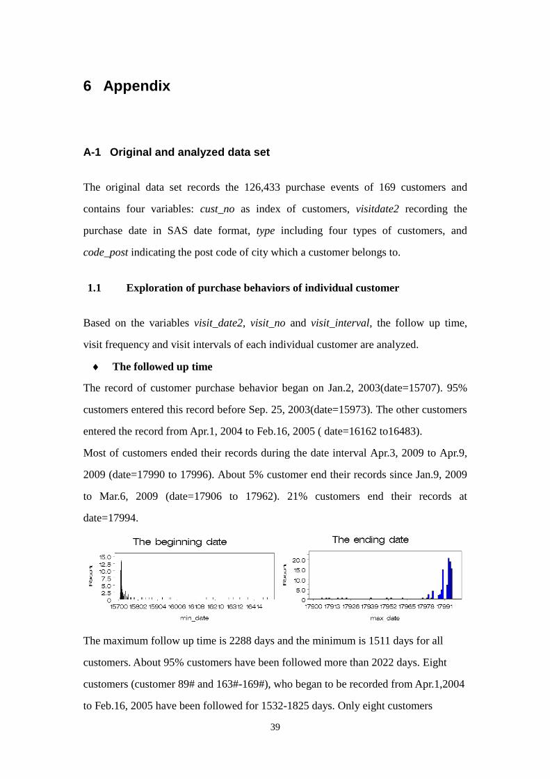
The followed up time

The record of customer purchase behavior began on Jan.2, 2003(date=15707). 95%

customers entered this record before Sep. 25, 2003(date=15973). The other customers

entered the record from Apr.1, 2004 to Feb.16, 2005 ( date=16162 to16483).

Most of customers ended their records during the date interval Apr.3, 2009 to Apr.9,

2009 (date=17990 to 17996). About 5% customer end their records since Jan.9, 2009

to Mar.6, 2009 (date=17906 to 17962). 21% customers end their records at

date=17994.

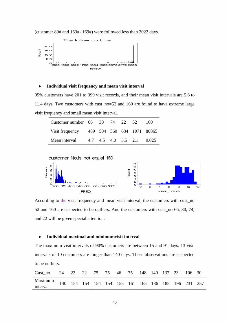
The maximum follow up time is 2288 days and the minimum is 1511 days for all

customers. About 95% customers have been followed more than 2022 days. Eight

customers (customer 89# and 163#-169#), who began to be recorded from Apr.1,2004

to Feb.16, 2005 have been followed for 1532-1825 days. Only eight customers

40

(customer 89# and 163#- 169#) were followed less than 2022 days.

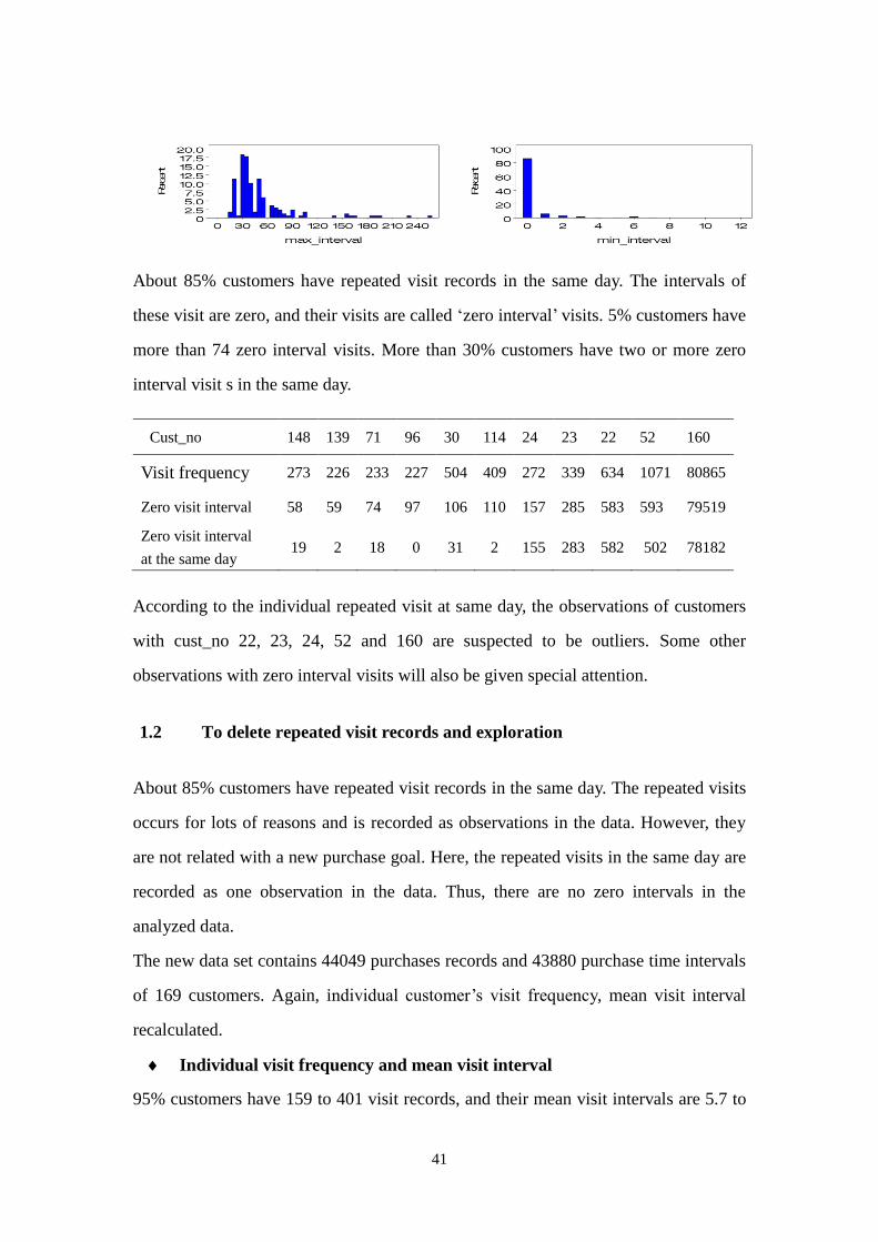
Individual visit frequency and mean visit interval

95% customers have 201 to 399 visit records, and their mean visit intervals are 5.6 to

11.4 days. Two customers with cust_no=52 and 160 are found to have extreme large

visit frequency and small mean visit interval.

Customer number 66 30 74 22 52 160

Visit frequency 489 504 560 634 1071 80865

Mean interval 4.7 4.5 4.0 3.5 2.1 0.025

According to the visit frequency and mean visit interval, the customers with cust_no

52 and 160 are suspected to be outliers. And the customers with cust_no 66, 30, 74,

and 22 will be given special attention.

Individual maximal and minimumvisit interval

The maximum visit intervals of 90% customers are between 15 and 91 days. 13 visit

intervals of 10 customers are longer than 140 days. These observations are suspected

to be outliers.

Cust_no 24 22 22 75 75 46 75 148 140 137 23 106 30

Maximum

interval 140 154 154 154 154 155 161 165 186 188 196 231 257

41

About 85% customers have repeated visit records in the same day. The intervals of

these visit are zero, and their visits are called ‘zero interval’ visits. 5% customers have

more than 74 zero interval visits. More than 30% customers have two or more zero

interval visit s in the same day.

Cust_no 148 139 71 96 30 114 24 23 22 52 160

Visit frequency 273 226 233 227 504 409 272 339 634 1071 80865

Zero visit interval 58 59 74 97 106 110 157 285 583 593 79519

Zero visit interval

at the same day 19 2 18 0 31 2 155 283 582 502 78182

According to the individual repeated visit at same day, the observations of customers

with cust_no 22, 23, 24, 52 and 160 are suspected to be outliers. Some other

observations with zero interval visits will also be given special attention.

1.2 To delete repeated visit records and exploration

About 85% customers have repeated visit records in the same day. The repeated visits

occurs for lots of reasons and is recorded as observations in the data. However, they

are not related with a new purchase goal. Here, the repeated visits in the same day are

recorded as one observation in the data. Thus, there are no zero intervals in the

analyzed data.

The new data set contains 44049 purchases records and 43880 purchase time intervals

of 169 customers. Again, individual customer’s visit frequency, mean visit interval

recalculated.

Individual visit frequency and mean visit interval

95% customers have 159 to 401 visit records, and their mean visit intervals are 5.7 to

42

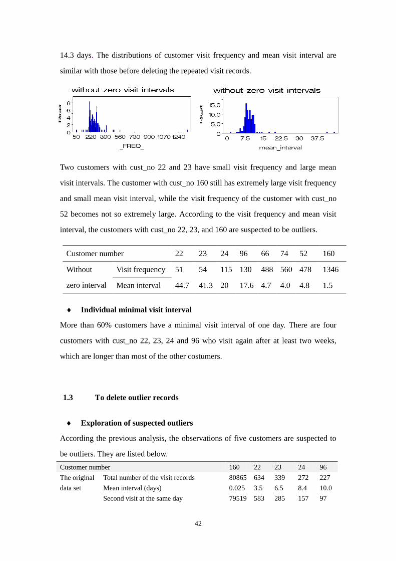
14.3 days. The distributions of customer visit frequency and mean visit interval are

similar with those before deleting the repeated visit records.

Two customers with cust_no 22 and 23 have small visit frequency and large mean

visit intervals. The customer with cust_no 160 still has extremely large visit frequency

and small mean visit interval, while the visit frequency of the customer with cust_no

52 becomes not so extremely large. According to the visit frequency and mean visit

interval, the customers with cust_no 22, 23, and 160 are suspected to be outliers.

Customer number 22 23 24 96 66 74 52 160

Without

zero interval

Visit frequency 51 54 115 130 488 560 478 1346

Mean interval 44.7 41.3 20 17.6 4.7 4.0 4.8 1.5

Individual minimal visit interval

More than 60% customers have a minimal visit interval of one day. There are four

customers with cust_no 22, 23, 24 and 96 who visit again after at least two weeks,

which are longer than most of the other costumers.

1.3 To delete outlier records

Exploration of suspected outliers

According the previous analysis, the observations of five customers are suspected to

be outliers. They are listed below.

Customer number 160 22 23 24 96

The original

data set

Total number of the visit records 80865 634 339 272 227

Mean interval (days) 0.025 3.5 6.5 8.4 10.0

Second visit at the same day 79519 583 285 157 97

43

At least the third visit at the same day 78182 582 283 155 0

The number of observations 126,433

Mean visit frequency for all customers 748 times

Mean visit interval for all customers 3.0 days

Mean visit frequency, except cust_no=160 271 times

Mean visit interval, except cust_no=160 8.3 days

The data set

without

repeated

visit records

Total number of the visit records 1346 51 54 115 130

Mean interval 1.5 44.7 41.3 20.0 17.6

The number of observations 44049

Mean visit frequency for all customers 261 times

Mean visit interval for all customers 8.6 days

Mean visit frequency, except cust_no=160 254 times

Mean visit interval, except cust_no=160 8.8 days

In the original data set, the customer with cust_no 160 has more than 60% of the visit

observations and extreme smaller mean visit interval than the others. After the

repeated visit records are deleted, this customer still has extremely larger visit

frequency and smaller mean visit interval than the others.

The customers with cust_no 22, 23 and 24, have many visit records in the same day

16369. There are 583 visit records for the customer 22 #, and 285 for the customer

23#, and 157 for the customer 24 #. After the repeated visit records are deleted, the

two customers have smaller visit frequencies and larger mean visit intervals than the

means.

The customers 24# and 96# do not behave extremely, even though their minimal visit

intervals are longer than those of the others (14 days).

To determine and delete the outliers

Based on the previous analysis, all observations of the customers with cust_no 160 are

removed as the outliers. And the observations of other four customers in the table will

be given special attention during the data analysis.

1.4 To define the observation time

Because right censored data is generally assumed to be valuable, the observation time

is defined to begin on January 2, 2003 ( date=15707) and end on March 31, 2009

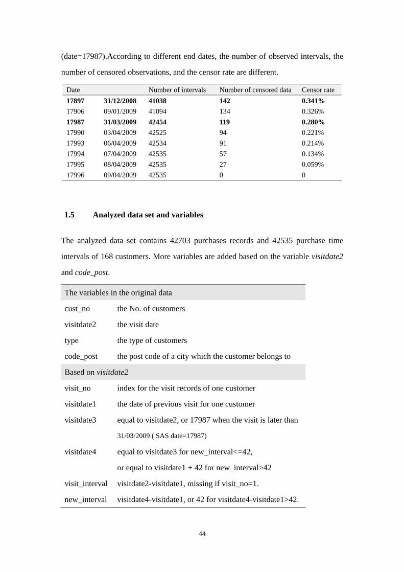
44

(date=17987).According to different end dates, the number of observed intervals, the

number of censored observations, and the censor rate are different.

Date Number of intervals Number of censored data Censor rate

17897 31/12/2008 41038 142 0.341%

17906 09/01/2009 41094 134 0.326%

17987 31/03/2009 42454 119 0.280%

17990 03/04/2009 42525 94 0.221%

17993 06/04/2009 42534 91 0.214%

17994 07/04/2009 42535 57 0.134%

17995 08/04/2009 42535 27 0.059%

17996 09/04/2009 42535 0 0

1.5 Analyzed data set and variables

The analyzed data set contains 42703 purchases records and 42535 purchase time

intervals of 168 customers. More variables are added based on the variable visitdate2

and code_post.

The variables in the original data

cust_no the No. of customers

visitdate2 the visit date

type the type of customers

code_post the post code of a city which the customer belongs to

Based on visitdate2

visit_no index for the visit records of one customer

visitdate1 the date of previous visit for one customer

visitdate3 equal to visitdate2, or 17987 when the visit is later than

31/03/2009 ( SAS date=17987)

visitdate4 equal to visitdate3 for new_interval<=42,

or equal to visitdate1 + 42 for new_interval>42

visit_interval visitdate2-visitdate1, missing if visit_no=1.

new_interval visitdate4-visitdate1, or 42 for visitdate4-visitdate1>42.

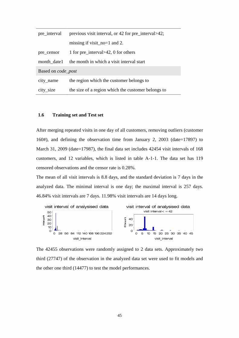
45

pre_interval previous visit interval, or 42 for pre_interval>42;

missing if visit_no=1 and 2.

pre_censor 1 for pre_interval>42, 0 for others

month_date1 the month in which a visit interval start

Based on code_post

city_name the region which the customer belongs to

city_size the size of a region which the customer belongs to

1.6 Training set and Test set

After merging repeated visits in one day of all customers, removing outliers (customer

160#), and defining the observation time from January 2, 2003 (date=17897) to

March 31, 2009 (date=17987), the final data set includes 42454 visit intervals of 168

customers, and 12 variables, which is listed in table A-1-1. The data set has 119

censored observations and the censor rate is 0.28%.

The mean of all visit intervals is 8.8 days, and the standard deviation is 7 days in the

analyzed data. The minimal interval is one day; the maximal interval is 257 days.

46.84% visit intervals are 7 days. 11.98% visit intervals are 14 days long.

The 42455 observations were randomly assigned to 2 data sets. Approximately two

third (27747) of the observation in the analyzed data set were used to fit models and

the other one third (14477) to test the model performances.

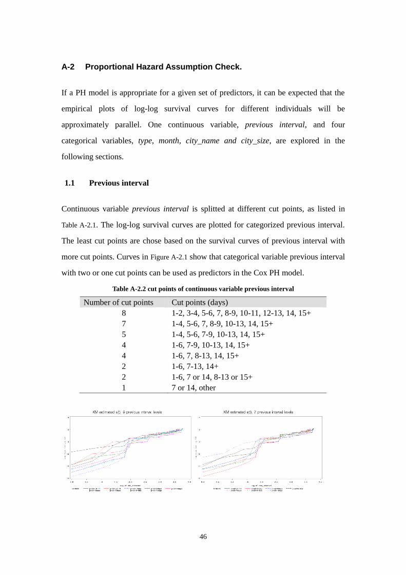
46

A-2 Proportional Hazard Assumption Check.

If a PH model is appropriate for a given set of predictors, it can be expected that the

empirical plots of log-log survival curves for different individuals will be

approximately parallel. One continuous variable, previous interval, and four

categorical variables, type, month, city_name and city_size, are explored in the

following sections.

1.1 Previous interval

Continuous variable previous interval is splitted at different cut points, as listed in

Table A-2.1. The log-log survival curves are plotted for categorized previous interval.

The least cut points are chose based on the survival curves of previous interval with

more cut points. Curves in Figure A-2.1 show that categorical variable previous interval

with two or one cut points can be used as predictors in the Cox PH model.

Table A-2.2 cut points of continuous variable previous interval

Number of cut points Cut points (days)

8 1-2, 3-4, 5-6, 7, 8-9, 10-11, 12-13, 14, 15+

7 1-4, 5-6, 7, 8-9, 10-13, 14, 15+

5 1-4, 5-6, 7-9, 10-13, 14, 15+

4 1-6, 7-9, 10-13, 14, 15+

4 1-6, 7, 8-13, 14, 15+

2 1-6, 7-13, 14+

2 1-6, 7 or 14, 8-13 or 15+

1 7 or 14, other

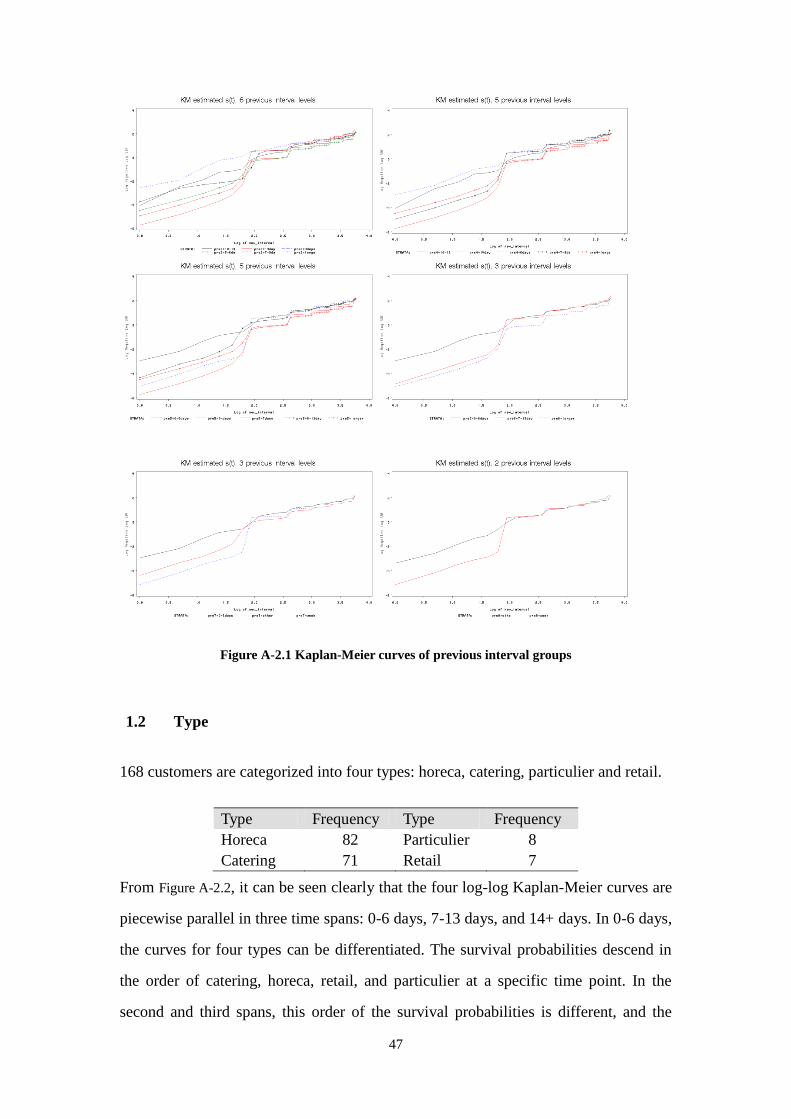
47

Figure A-2.1 Kaplan-Meier curves of previous interval groups

1.2 Type

168 customers are categorized into four types: horeca, catering, particulier and retail.

Type Frequency Type Frequency

Horeca 82 Particulier 8

Catering 71 Retail 7

From Figure A-2.2, it can be seen clearly that the four log-log Kaplan-Meier curves are

piecewise parallel in three time spans: 0-6 days, 7-13 days, and 14+ days. In 0-6 days,

the curves for four types can be differentiated. The survival probabilities descend in

the order of catering, horeca, retail, and particulier at a specific time point. In the

second and third spans, this order of the survival probabilities is different, and the

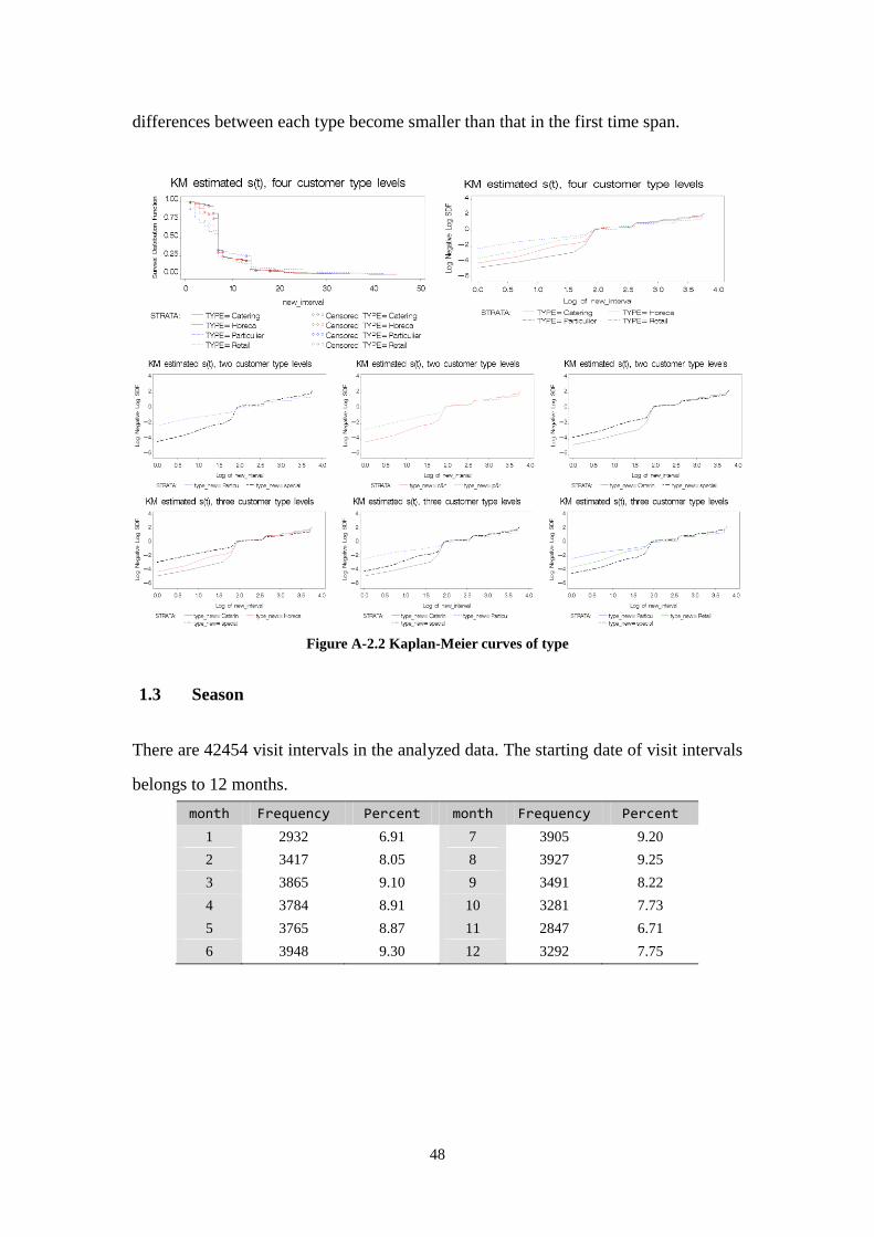
48

differences between each type become smaller than that in the first time span.

Figure A-2.2 Kaplan-Meier curves of type

1.3 Season

There are 42454 visit intervals in the analyzed data. The starting date of visit intervals

belongs to 12 months.

month Frequency Percent month Frequency Percent

1 2932 6.91 7 3905 9.20

2 3417 8.05 8 3927 9.25

3 3865 9.10 9 3491 8.22

4 3784 8.91 10 3281 7.73

5 3765 8.87 11 2847 6.71

6 3948 9.30 12 3292 7.75

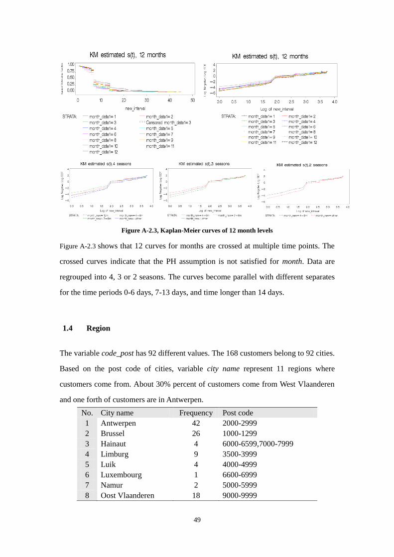
49

Figure A-2.3, Kaplan-Meier curves of 12 month levels

Figure A-2.3 shows that 12 curves for months are crossed at multiple time points. The

crossed curves indicate that the PH assumption is not satisfied for month. Data are

regrouped into 4, 3 or 2 seasons. The curves become parallel with different separates

for the time periods 0-6 days, 7-13 days, and time longer than 14 days.

1.4 Region

The variable code_post has 92 different values. The 168 customers belong to 92 cities.

Based on the post code of cities, variable city name represent 11 regions where

customers come from. About 30% percent of customers come from West Vlaanderen

and one forth of customers are in Antwerpen.

No. City name Frequency Post code

1 Antwerpen 42 2000-2999

2 Brussel 26 1000-1299

3 Hainaut 4 6000-6599,7000-7999

4 Limburg 9 3500-3999

5 Luik 4 4000-4999

6 Luxembourg 1 6600-6999

7 Namur 2 5000-5999

8 Oost Vlaanderen 18 9000-9999

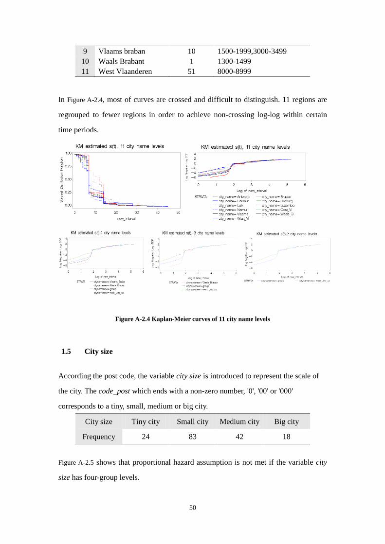
50

9 Vlaams braban 10 1500-1999,3000-3499

10 Waals Brabant 1 1300-1499

11 West Vlaanderen 51 8000-8999

In Figure A-2.4, most of curves are crossed and difficult to distinguish. 11 regions are

regrouped to fewer regions in order to achieve non-crossing log-log within certain

time periods.

Figure A-2.4 Kaplan-Meier curves of 11 city name levels

1.5 City size

According the post code, the variable city size is introduced to represent the scale of

the city. The code_post which ends with a non-zero number, '0', '00' or '000'

corresponds to a tiny, small, medium or big city.

City size Tiny city Small city Medium city Big city

Frequency 24 83 42 18

Figure A-2.5 shows that proportional hazard assumption is not met if the variable city

size has four-group levels.

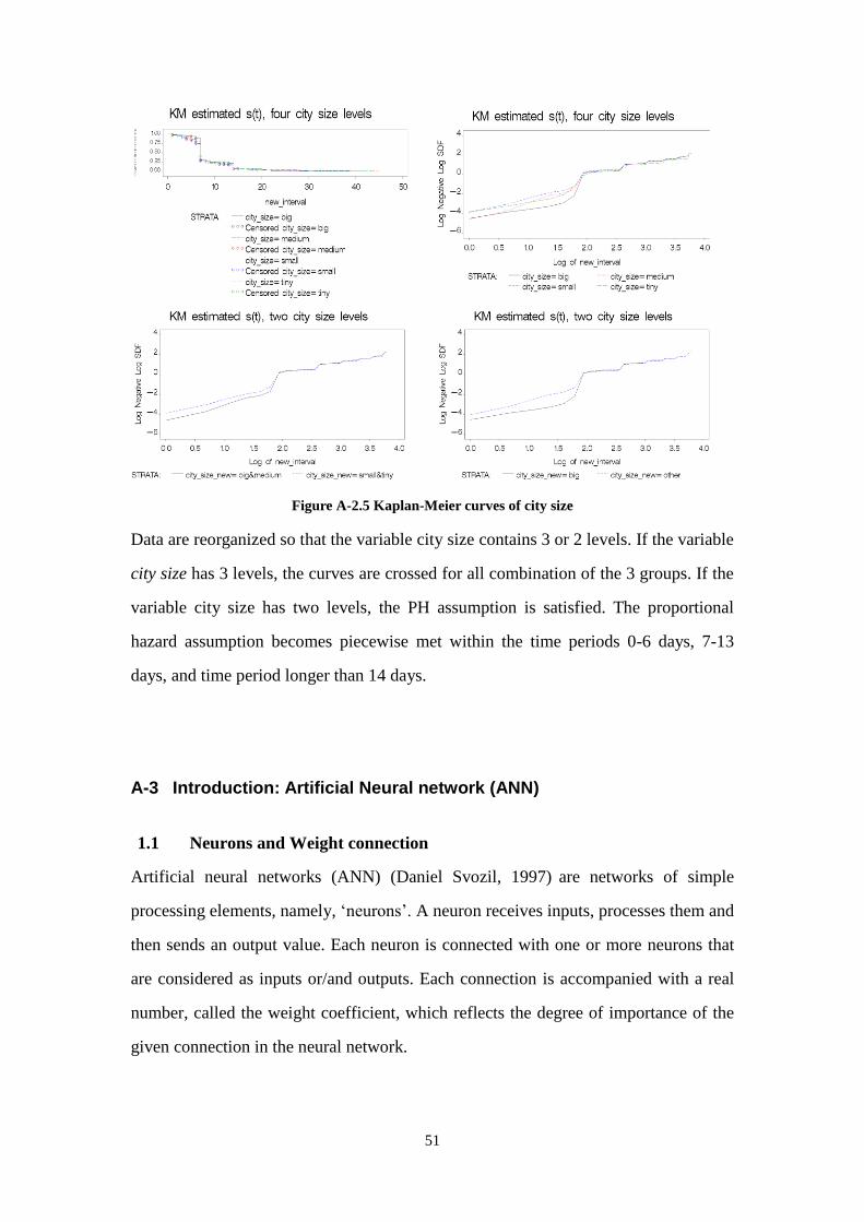
51

Figure A-2.5 Kaplan-Meier curves of city size

Data are reorganized so that the variable city size contains 3 or 2 levels. If the variable

city size has 3 levels, the curves are crossed for all combination of the 3 groups. If the

variable city size has two levels, the PH assumption is satisfied. The proportional

hazard assumption becomes piecewise met within the time periods 0-6 days, 7-13

days, and time period longer than 14 days.

A-3 Introduction: Artificial Neural network (ANN)

1.1 Neurons and Weight connection

Artificial neural networks (ANN) (Daniel Svozil, 1997) are networks of simple

processing elements, namely, ‘neurons’. A neuron receives inputs, processes them and

then sends an output value. Each neuron is connected with one or more neurons that

are considered as inputs or/and outputs. Each connection is accompanied with a real

number, called the weight coefficient, which reflects the degree of importance of the

given connection in the neural network.

52

1.2 Multi-layer feed-forward (MLF) neural network

Multi-layer feed-forward (MLF) neural network is the most popular neural network

(Daniel Svozil, 1997) . The neurons of a MLF neural network are ordered to an input

layer, one or more intermediate hidden layers, and an output layer. Each neuron in a

hidden layer computes a weighted sum of the inputs ip with weights ijw , , adds a

constant jb (bias), and applies an activation function f( ) to obtain its output,

expressed as the equation (A-3.1).

R

i

jiijj wpbfa1

)( (A-3.1)

The outputs of the last hidden layer become the inputs of the output layer nodes; their

outputs are computed in the same way as an intermediate hidden layer with weights

khw , , bias k and activation 0f . The kth

output in the output layer is expressed as:

S

h

hhkkk awfy1

0 )(ˆ (A-3.2)

An example of NN is illustrated in Figure A-3.1.

Figure A-3.1 One hidden layer of a MLF neural network

1.3 Training a neural network

Generally, neural networks are adjusted or trained until some conditions are fulfilled.

There are two main types of training processes involving supervised and unsupervised

training. Supervised training means that neural network knows the desired output, and

it adjusts the weight coefficients given the condition that the calculated outputs and

53

the desired outputs are as close as possible. On the other hand, unsupervised training

means that the desired output is unknown, and is automatically optimized to reach a

stable state by an iterative algorithm.

MLF neural network is a supervised training network. The network is adjusted in an

iterative way judging from a comparison between the output and the target until the

network output matches the target (Daniel Svozil, 1997).

Figure A-3.2 The training of a network

In practice, the weights (parameters of the neural network model) are estimated by

minimizing an appropriate error function. The most frequently used error function is

the quadratic error function with the equation form as:

K

k

I

i

kiik ywxyE1 1

2)),(ˆ( (A-3.3)

The cross-entropy error function is applied for binary classification problems. This

error function is expressed as:

K

k

n

i

ikikikik wxyywxyyE1 1

)],(ˆ1log[)1()),(ˆlog( (A-3.4)

Several techniques can be applied to modulate the degree in fitting a neural network.

These techniques include the choice of the number of hidden nodes (neurons), the use

of regularization techniques, the addition of a penalty term to the error function, and

an early stop during the iteration of the optimization algorithm.

1.4 Neural network survival analysis

An example with two observations shown in Table 2.3.1 illustrates those modification

strategies on the data structures. The case includes two covariates X1 and X2. The

54

subject A was censored on the third day, and the subject B fails on the fourth day. The

total follow-up time is 5 days.

Table A-3.1 A case to illustrate the different data structures

No. X1 X2 Survival time Censor

A 1 0 3 days 1

B 1 1 4 days 0

K. Liestol, P. K. Andersen and U. Andersen

The approach mentioned by Liestol et al. was based on the modification of Cox

proportional odds model (K. Liestol, 1994). For grouped survival data, the observe

time T is categorized into K disjoint intervals. The proportional odds model is

expressed as:

Kkh

h

h

hi

T

k

k

ikl

ik 2,1)exp()0(1

)0(

)(1

)(

x

x

x (A-3.5)

A logistic regression model is derived from the Cox proportional odds model:

])0(1

)0(log[

)exp(1

)exp()(

k

kk

i

T

k

i

T

kik

h

hxh

x

x (A-3.6)

Thus the discrete hazard rates are modeled by a logistic regression model adhering to

a predictor, which is a linear combination of covariate values.

In this case, the total follow-up time is divided into five time intervals: the first day,

the second day, the third day, the 4th

day and the 5th

day. The structure of the

transformed data is listed in table A-3.2.

Table A-3.2 The data structure is transformed by the method suggested by Liestol et al. (K.

Liestol, 1994).

No ANN input Target: survival status in discrete time intervals

X1 X2 day 1 day 2 day 3 day 4 day 5

A 1 0 0 0 0 / /

B 1 1 0 0 0 1 /

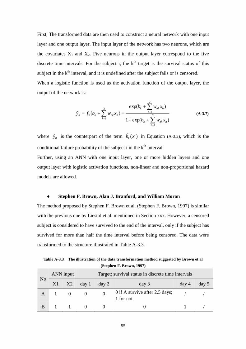
55

First, The transformed data are then used to construct a neural network with one input

layer and one output layer. The input layer of the network has two neurons, which are

the covariates X1 and X2. Five neurons in the output layer correspond to the five

discrete time intervals. For the subject i, the kth

target is the survival status of this

subject in the kth

interval, and it is undefined after the subject fails or is censored.

When a logistic function is used as the activation function of the output layer, the

output of the network is:

2

1

2

12

1

0

)exp(1

)exp(

)(ˆ

h

hhkk

h

hhkk

h

hhkkk

xwb

xwb

xwbfy (A-3.7)

where iky is the counterpart of the term )(ˆik xh in Equation (A-3.2), which is the

conditional failure probability of the subject i in the kth

interval.

Further, using an ANN with one input layer, one or more hidden layers and one

output layer with logistic activation functions, non-linear and non-proportional hazard

models are allowed.

Stephen F. Brown, Alan J. Branford, and William Moran

The method proposed by Stephen F. Brown et al. (Stephen F. Brown, 1997) is similar

with the previous one by Liestol et al. mentioned in Section xxx. However, a censored

subject is considered to have survived to the end of the interval, only if the subject has

survived for more than half the time interval before being censored. The data were

transformed to the structure illustrated in Table A-3.3.

Table A-3.3 The illustration of the data transformation method suggested by Brown et al

(Stephen F. Brown, 1997)

No ANN input Target: survival status in discrete time intervals

X1 X2 day 1 day 2 day 3 day 4 day 5

A 1 0 0 0 0 if A survive after 2.5 days;

1 for not / /

B 1 1 0 0 0 1 /

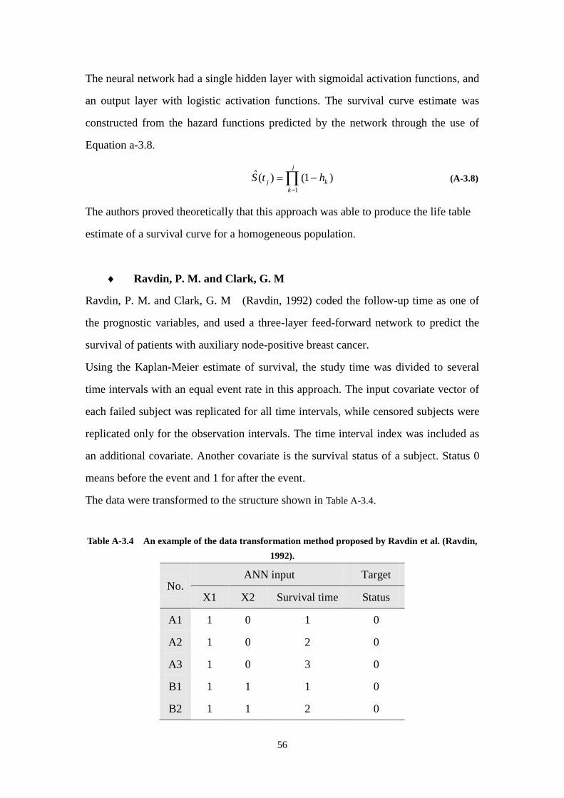
56

The neural network had a single hidden layer with sigmoidal activation functions, and

an output layer with logistic activation functions. The survival curve estimate was

constructed from the hazard functions predicted by the network through the use of

Equation a-3.8.

)1()(ˆ

1

k

j

k

j htS

(A-3.8)

The authors proved theoretically that this approach was able to produce the life table

estimate of a survival curve for a homogeneous population.

Ravdin, P. M. and Clark, G. M

Ravdin, P. M. and Clark, G. M (Ravdin, 1992) coded the follow-up time as one of

the prognostic variables, and used a three-layer feed-forward network to predict the

survival of patients with auxiliary node-positive breast cancer.

Using the Kaplan-Meier estimate of survival, the study time was divided to several

time intervals with an equal event rate in this approach. The input covariate vector of

each failed subject was replicated for all time intervals, while censored subjects were

replicated only for the observation intervals. The time interval index was included as

an additional covariate. Another covariate is the survival status of a subject. Status 0

means before the event and 1 for after the event.

The data were transformed to the structure shown in Table A-3.4.

Table A-3.4 An example of the data transformation method proposed by Ravdin et al. (Ravdin,

1992).

No. ANN input Target

X1 X2 Survival time Status

A1 1 0 1 0

A2 1 0 2 0

A3 1 0 3 0

B1 1 1 1 0

B2 1 1 2 0

57

B3 1 1 3 0

B4 1 1 4 1

B5 1 1 5 1

One replicated input vector was one input of the neural network. The output layer of

the network had only one neuron and the target value was the survival status, which

was either 0 or 1. Hyperbolic tangent functions were used in the hidden and output

layers. The actual output value varied from 0 to 1. The authors stated that the output

of the neural network was roughly proportional to the Kaplan-Meier estimate of the

survival probability.