networks ch_03.ppt

7/27/2019 networks ch_03.ppt

http://slidepdf.com/reader/full/networks-ch03ppt 1/77

McGraw-Hill ©The McGraw-Hill Companies, Inc., 2004

Physical Layer

PART II




Position of the physical layer



Services




Chapters

Chapter 3 Signals

Chapter 4 Digital Transmission

Chapter 5 Analog Transmission

Chapter 6 Multiplexing

Chapter 7 Transmission M edia

Chapter 8 Circuit Switching and Telephone Network

Chapter 9 H igh Speed Digital Access




Chapter 3

Signals




To be transmi tted, data must be

transformed to electromagnetic signals.

Note:


http://slidepdf.com/reader/full/networks-ch03ppt 7/77McGraw-Hill ©The McGraw-Hill Companies, Inc., 2004

3.1 Analog and Digital

Analog and Digital Data

Analog and Digital Signals

Periodic and Aperiodic Signals



Signals can be analog or digital.

Analog signals can have an inf inite number of values in a range; digital

signals can have only a limited

number of values.

Note:



Figure 3.1 Comparison of analog and digital signals



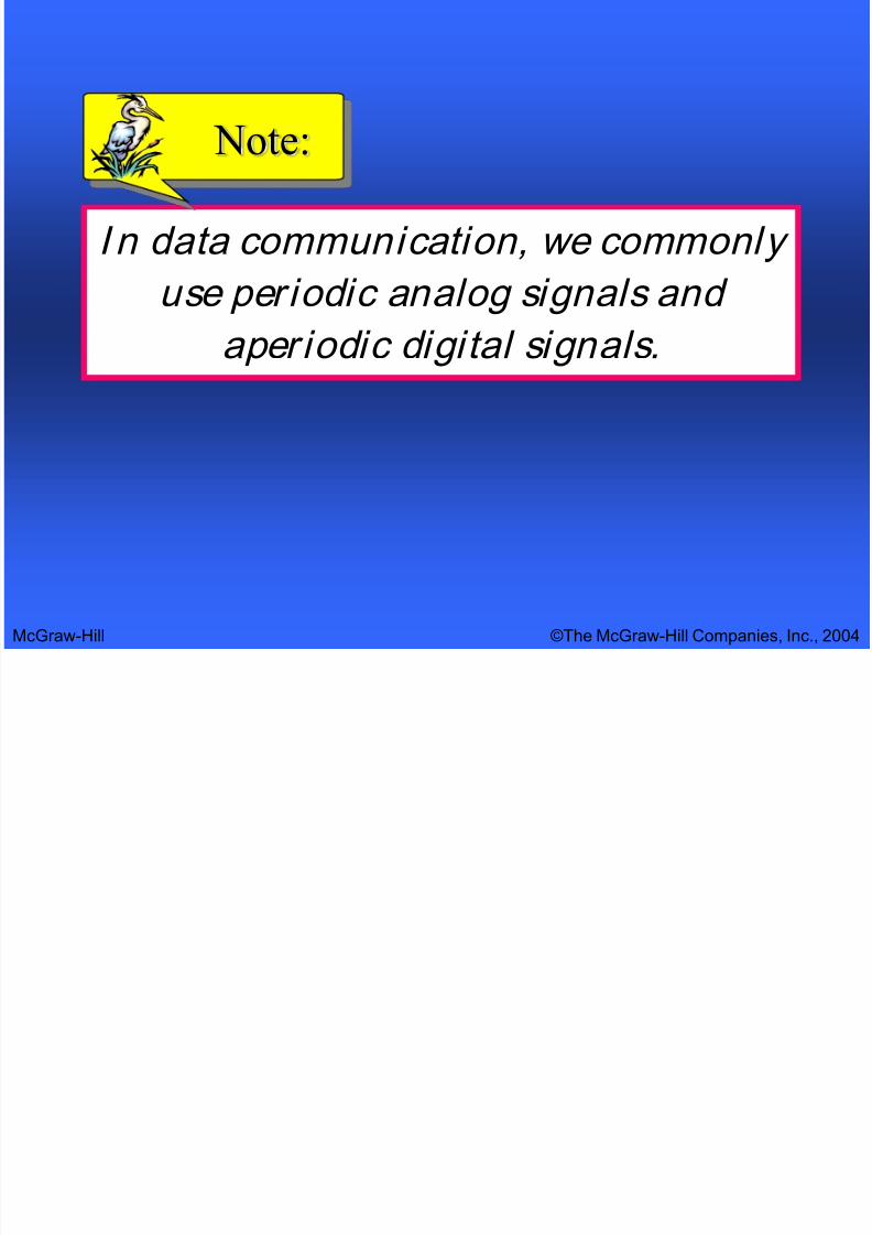
I n data communication, we commonly

use periodic analog signals and aper iodic digital signals.

Note:



3.2 Analog Signals

Sine Wave

Phase

Examples of Sine Waves

Time and Frequency Domains

Composite Signals Bandwidth



Figure 3.2 A sine wave



Figure 3.3 Amplitude



Frequency and period are inverses of

each other.

Note:



Figure 3.4 Period and frequency



Table 3.1 Uni ts of per iods and frequencies

Unit Equivalent Unit Equivalent

Seconds (s) 1 s hertz (Hz) 1 Hz

Milliseconds (ms) 10 – 3 s kilohertz (KHz) 103 Hz

Microseconds (ms) 10 – 6 s megahertz (MHz) 106 Hz

Nanoseconds (ns) 10 – 9 s gigahertz (GHz) 109 Hz

Picoseconds (ps) 10 – 12 s terahertz (THz) 1012 Hz



Example 1

Express a period of 100 ms in microseconds, and express

the corresponding frequency in kilohertz.

Solution

From Table 3.1 we find the equivalent of 1 ms.We makethe following substitutions:

100 ms = 100 10-3 s = 100 10-3 106 ms = 105 ms

Now we use the inverse relationship to find thefrequency, changing hertz to kilohertz

100 ms = 100 10-3 s = 10-1 s

f = 1/10-1 Hz = 10 10-3 KHz = 10-2 KHz



Frequency is the rate of change with

respect to time. Change in a short span of time means high f requency. Change

over a long span of time means low

frequency.

Note:



I f a signal does not change at all, its

frequency is zero. I f a signal changes instantaneously, its frequency is

infinite.

Note:



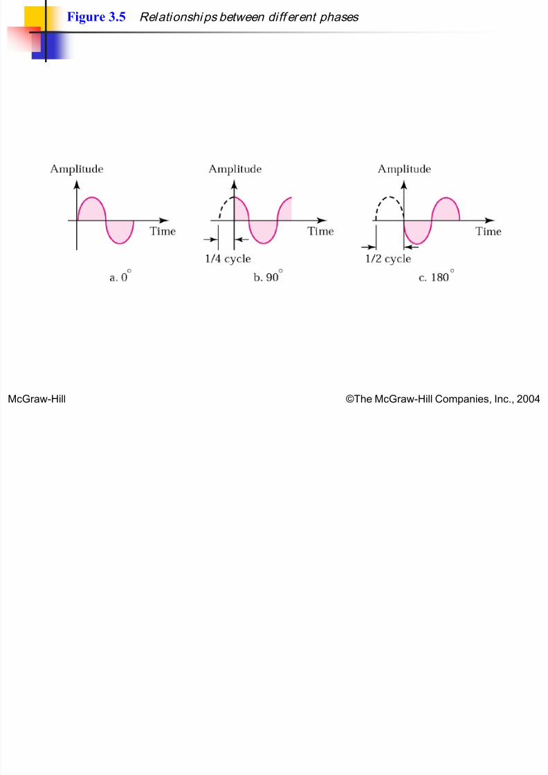
Phase describes the position of the

waveform relative to time zero.

Note:



Figure 3.5 Relationships between diff erent phases




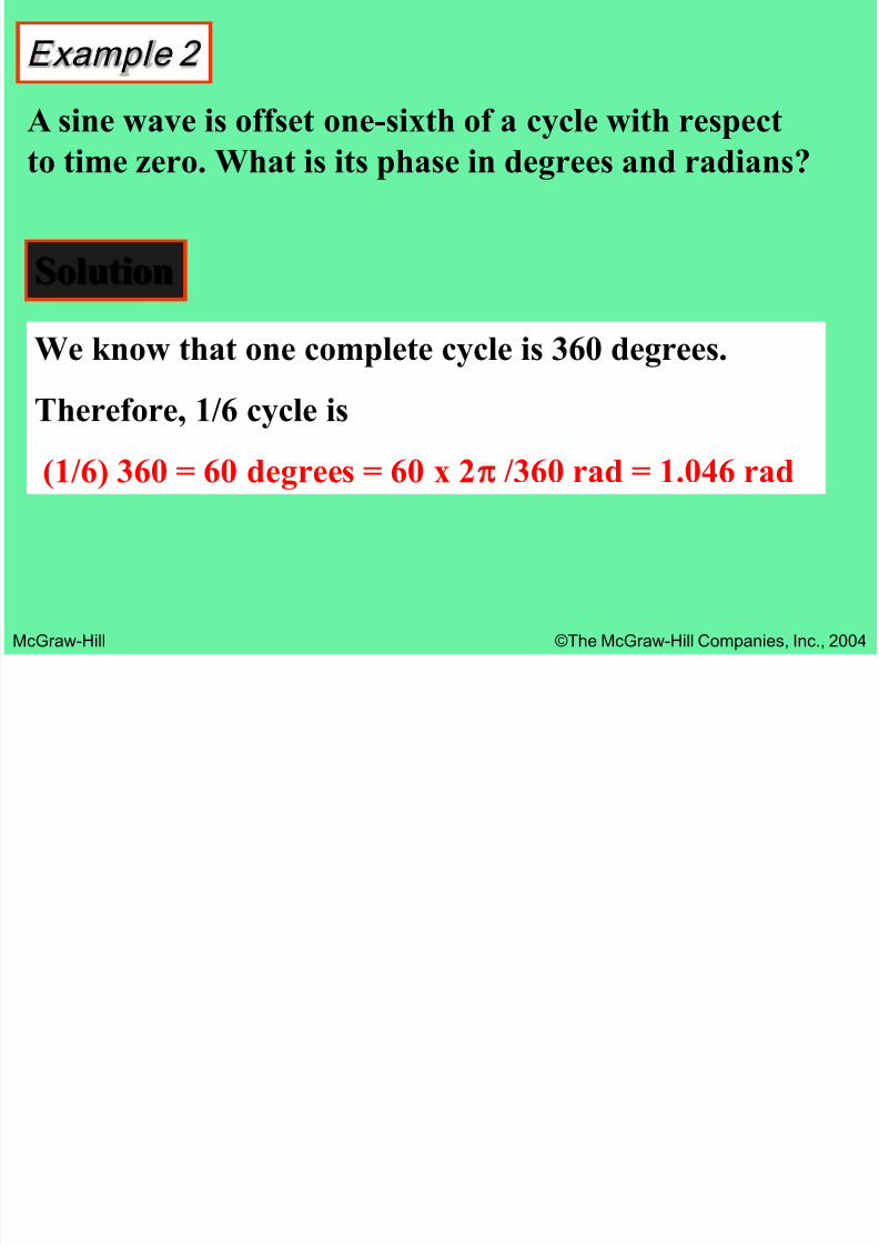
Example 2

A sine wave is offset one-sixth of a cycle with respect

to time zero. What is its phase in degrees and radians?

Solution

We know that one complete cycle is 360 degrees.

Therefore, 1/6 cycle is

(1/6) 360 = 60 degrees = 60 x 2p /360 rad = 1.046 rad




Figure 3.6 Sine wave examples




Figure 3.6 Sine wave examples (continued)




Figure 3.6 Sine wave examples (continued)




An analog signal is best represented in

the frequency domain.

Note:

Fi 3 7 f




Figure 3.7 Time and f requency domains

Fi 3 7 Ti d f d i ( ti d)




Figure 3.7 Time and frequency domains (continued)

Fi 3 7 Ti d f d i ( ti d)




Figure 3.7 Time and frequency domains (continued)




A single-f requency sine wave is not

useful in data communications; we need to change one or more of its

character istics to make it useful.

Note:




When we change one or more

character istics of a single-f requency signal, it becomes a composite signal

made of many frequencies.

Note:




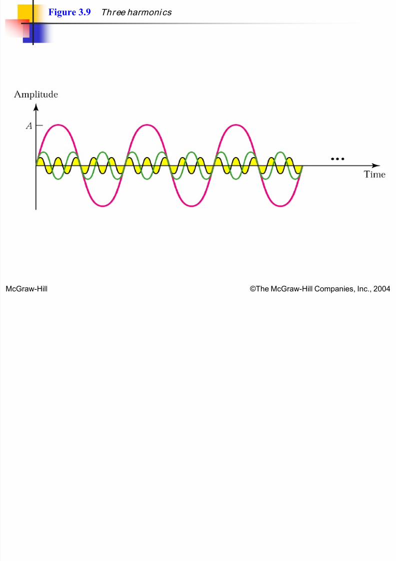
According to Four ier analysis, any

composite signal can be represented as a combination of simple sine waves

with different f requencies, phases, and

amplitudes.

Note:

Figure 3 8 Square wave




Figure 3.8 Square wave

Figure 3 9 Three harmonics




Figure 3.9 Three harmonics

Figure 3 10 Adding f irst three harmonics




Figure 3.10 Adding f irst three harmonics

Figure 3 11 Frequency spectrum comparison




Figure 3.11 Frequency spectrum comparison

Figure 3 12 Signal corr uption




Figure 3.12 Signal corr uption




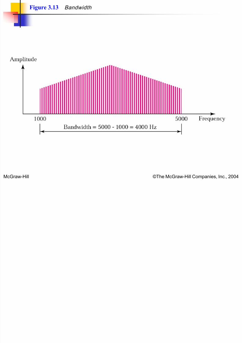
The bandwidth is a property of a

medium: I t is the difference between the highest and the lowest frequencies

that the medium can

satisfactor i ly pass.

Note:




I n this book, we use the term

bandwidth to refer to the property of a medium or the width of a single

spectrum.

Note:

Figure 3 13 Bandwidth




Figure 3.13 Bandwidth




Example 3

If a periodic signal is decomposed into five sine waves

with frequencies of 100, 300, 500, 700, and 900 Hz,what is the bandwidth? Draw the spectrum, assuming all

components have a maximum amplitude of 10 V.

Solution

B = f h - f l = 900 - 100 = 800 Hz

The spectrum has only five spikes, at 100, 300, 500, 700,and 900 (see Figure 13.4 )

Figure 3.14 Example 3








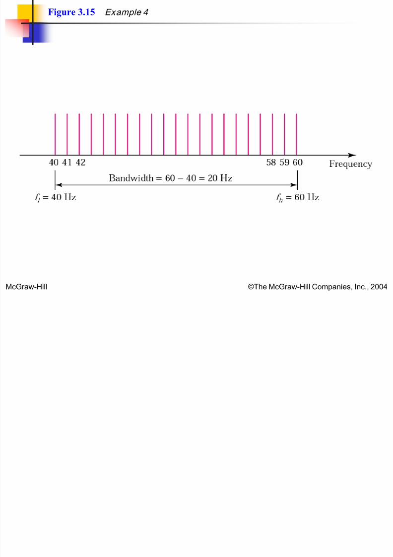
Example 4

A signal has a bandwidth of 20 Hz. The highest frequency

is 60 Hz. What is the lowest frequency? Draw thespectrum if the signal contains all integral frequencies of

the same amplitude.

Solution

B = f h - f l

20 = 60 - f l

f l = 60 - 20 = 40 Hz









Example 5

A signal has a spectrum with frequencies between 1000

and 2000 Hz (bandwidth of 1000 Hz). A medium can passfrequencies from 3000 to 4000 Hz (a bandwidth of 1000

Hz). Can this signal faithfully pass through this medium?

Solution

The answer is definitely no. Although the signal can havethe same bandwidth (1000 Hz), the range does not

overlap. The medium can only pass the frequencies

between 3000 and 4000 Hz; the signal is totally lost.




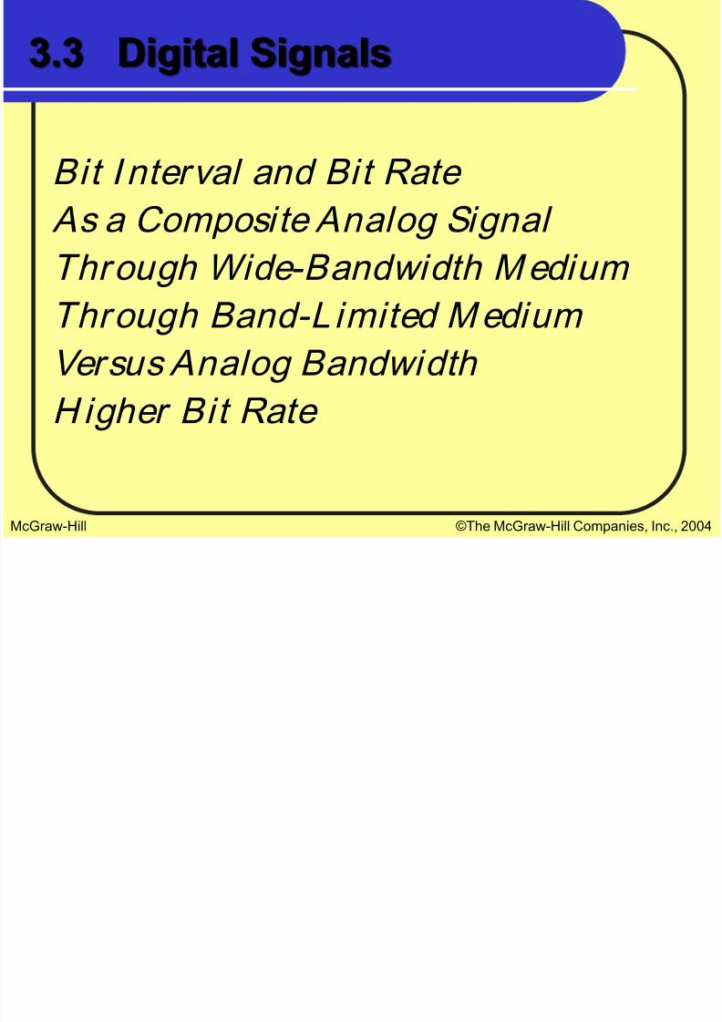
3.3 Digital Signals

Bit I nterval and Bit Rate

As a Composite Analog Signal

Through Wide-Bandwidth Medium

Through Band-L imited Medium

Versus Analog Bandwidth

H igher Bit Rate

Figure 3.16 A digital signal




g g g




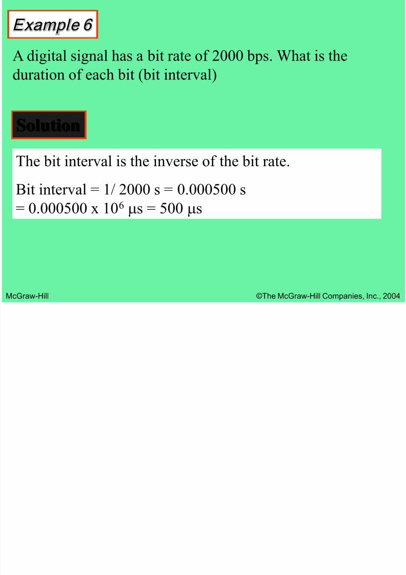
Example 6

A digital signal has a bit rate of 2000 bps. What is the

duration of each bit (bit interval)

Solution

The bit interval is the inverse of the bit rate.

Bit interval = 1/ 2000 s = 0.000500 s

= 0.000500 x 10

6

ms = 500 ms

Figure 3.17 Bi t rate and bit interval




g

Figure 3.18 Digital versus analog







A digital signal is a composite signal

with an inf ini te bandwidth.

Note:




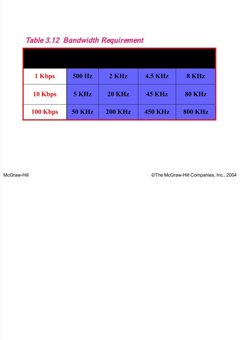
Table 3.12 Bandwidth Requirement

Bit

Rate

Harmonic

1

Harmonics

1, 3

Harmonics

1, 3, 5

Harmonics

1, 3, 5, 7

1 Kbps 500 Hz 2 KHz 4.5 KHz 8 KHz

10 Kbps 5 KHz 20 KHz 45 KHz 80 KHz

100 Kbps 50 KHz 200 KHz 450 KHz 800 KHz




The bit rate and the bandwidth are

proportional to each other.

Note:




3.4 Analog versus Digital

Low-pass versus Band-pass

Digital Transmission

Analog Transmission

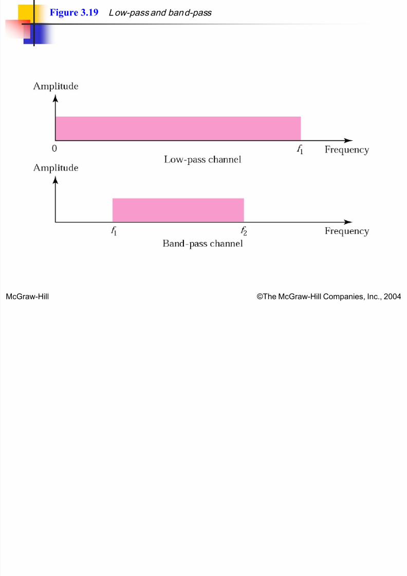
Figure 3.19 Low-pass and band-pass







The analog bandwidth of a medium is

expressed in hertz; the digital

bandwidth, in bits per second.

Note:




Digital transmission needs a

low-pass channel.

Note:




Analog transmission can use a band-

pass channel.

Note:

3 5 D R Li i




3.5 Data Rate Limit

Noiseless Channel: Nyquist Bit Rate

Noisy Channel: Shannon Capacity

Using Both L imits

E ample 7




Example 7

Consider a noiseless channel with a bandwidth of 3000

Hz transmitting a signal with two signal levels. Themaximum bit rate can be calculated as

Bit Rate = 2 3000 log2 2 = 6000 bps

Example 8




Example 8

Consider the same noiseless channel, transmitting a signal

with four signal levels (for each level, we send two bits).The maximum bit rate can be calculated as:

Bit Rate = 2 x 3000 x log2 4 = 12,000 bps

Example 9




Example 9

Consider an extremely noisy channel in which the value

of the signal-to-noise ratio is almost zero. In other words,the noise is so strong that the signal is faint. For this

channel the capacity is calculated as

C = B log2 (1 + SNR) = B log2 (1 + 0)

= B log2 (1) = B 0 = 0

Example 10




Example 10

We can calculate the theoretical highest bit rate of a

regular telephone line. A telephone line normally has a bandwidth of 3000 Hz (300 Hz to 3300 Hz). The signal-

to-noise ratio is usually 3162. For this channel the

capacity is calculated as

C = B log2 (1 + SNR) = 3000 log2 (1 + 3162)

= 3000 log2 (3163)

C = 3000 11.62 = 34,860 bps

Example 11




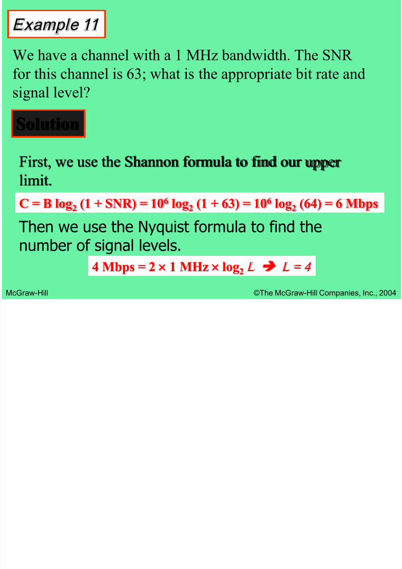
Example 11

We have a channel with a 1 MHz bandwidth. The SNR

for this channel is 63; what is the appropriate bit rate andsignal level?

Solution

C = B log2 (1 + SNR) = 106 log2 (1 + 63) = 106 log2 (64) = 6 Mbps

Then we use the Nyquist formula to find thenumber of signal levels.

4 Mbps = 2 1 MHz log2 L L = 4

First, we use the Shannon formula to find our upper

limit.

3 6 T i i I i t




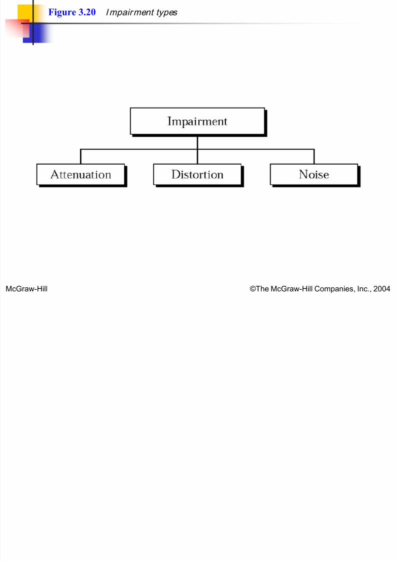
3.6 Transmission Impairment

Attenuation

Distortion

Noise

Figure 3.20 Impairment types




Figure 3.21 Attenuation




Example 12




Example 12

Imagine a signal travels through a transmission medium

and its power is reduced to half. This means that P2 = 1/2P1. In this case, the attenuation (loss of power) can be

calculated as

Solution

10 log10 (P2/P1) = 10 log10 (0.5P1/P1) = 10 log10 (0.5)

= 10( – 0.3) = – 3 dB

Example 13




Example 13

Imagine a signal travels through an amplifier and its

power is increased ten times. This means that P2 = 10 ¥P1. In this case, the amplification (gain of power) can be

calculated as

10 log10 (P2/P1) = 10 log10 (10P1/P1)

= 10 log10 (10) = 10 (1) = 10 dB

Example 14




Example 14

One reason that engineers use the decibel to measure the

changes in the strength of a signal is that decibel numberscan be added (or subtracted) when we are talking about

several points instead of just two (cascading). In Figure

3.22 a signal travels a long distance from point 1 to point

4. The signal is attenuated by the time it reaches point 2.Between points 2 and 3, the signal is amplified. Again,

between points 3 and 4, the signal is attenuated. We can

find the resultant decibel for the signal just by adding the

decibel measurements between each set of points.





dB = –

3 + 7 –

3 = +1

Figure 3.23 Distortion




Figure 3.24 Noise




3 7 More About Signals




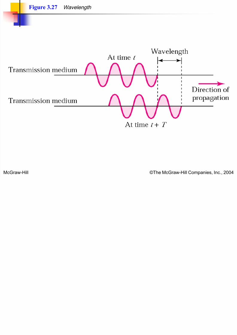
3.7 More About Signals

Throughput

Propagation Speed

Propagation Time

Wavelength

Figure 3.25 Throughput




Figure 3.26 Propagation time




Figure 3.27 Wavelength



networks ch_03.ppt

Documents