FPO 9 Network Theorems Network Theorems 9.1 INTRODUCTION This chapter introduces a number of theorems that have application throughout the field of electricity and electronics. Not only can they be used to solve networks such as encountered in the previous chapter, but they also provide an opportunity to determine the impact of a particular source or element on the response of the entire system. In most cases, the network to be analyzed and the mathematics required to find the solution are simplified. All of the theorems appear again in the analysis of ac networks. In fact, the application of each theorem to ac networks is very similar in content to that found in this chapter. The first theorem to be introduced is the superposition theorem, followed by Thévenin’s theorem, Norton’s theorem, and the maximum power transfer theorem. The chapter concludes with a brief introduction to Millman’s theorem and the substitution and reciprocity theorems. 9.2 SUPERPOSITION THEOREM The superposition theorem is unquestionably one of the most powerful in this field. It has such widespread application that people often apply it without recognizing that their maneu- vers are valid only because of this theorem. In general, the theorem can be used to do the following: • Analyze networks such as introduced in the last chapter that have two or more sources that are not in series or parallel. • Reveal the effect of each source on a particular quantity of interest. • For sources of different types (such as dc and ac, which affect the parameters of the network in a different manner) and apply a separate analysis for each type, with the total result simply the algebraic sum of the results. • Become familiar with the superposition theorem and its unique ability to separate the impact of each source on the quantity of interest. • Be able to apply Thévenin’s theorem to reduce any two-terminal, series-parallel network with any number of sources to a single voltage source and series resistor. • Become familiar with Norton’s theorem and how it can be used to reduce any two-terminal, series- parallel network with any number of sources to a single current source and a parallel resistor. • Understand how to apply the maximum power transfer theorem to determine the maximum power to a load and to choose a load that will receive maximum power. • Become aware of the reduction powers of Millman’s theorem and the powerful implications of the substitution and reciprocity theorems. Objectives 9 Th GRIDLINE SET IN 1ST-PP TO INDICATE SAFE AREA; TO BE REMOVED AFTER 1ST-PP

Welcome message from author
This document is posted to help you gain knowledge. Please leave a comment to let me know what you think about it! Share it to your friends and learn new things together.
Transcript

FPO
9Network TheoremsNetwork Theorems
9.1 INTRODUCTION
This chapter introduces a number of theorems that have application throughout the field of electricity and electronics. Not only can they be used to solve networks such as encountered in the previous chapter, but they also provide an opportunity to determine the impact of a particular source or element on the response of the entire system. In most cases, the network to be analyzed and the mathematics required to find the solution are simplified. All of the theorems appear again in the analysis of ac networks. In fact, the application of each theorem to ac networks is very similar in content to that found in this chapter.
The first theorem to be introduced is the superposition theorem, followed by Thévenin’s theorem, Norton’s theorem, and the maximum power transfer theorem. The chapter concludes with a brief introduction to Millman’s theorem and the substitution and reciprocity theorems.
9.2 SUPERPOSITION THEOREM
The superposition theorem is unquestionably one of the most powerful in this field. It has such widespread application that people often apply it without recognizing that their maneu-vers are valid only because of this theorem.
In general, the theorem can be used to do the following:
• Analyze networks such as introduced in the last chapter that have two or more sources that are not in series or parallel.
• Reveal the effect of each source on a particular quantity of interest.• For sources of different types (such as dc and ac, which affect the parameters of the
network in a different manner) and apply a separate analysis for each type, with the total result simply the algebraic sum of the results.
• Become familiar with the superposition theorem and its unique ability to separate the impact of each source on the quantity of interest.
• Be able to apply Thévenin’s theorem to reduce any two-terminal, series-parallel network with any number of sources to a single voltage source and series resistor.
• Become familiar with Norton’s theorem and how it can be used to reduce any two-terminal, series-parallel network with any number of sources to a single current source and a parallel resistor.
• Understand how to apply the maximum power transfer theorem to determine the maximum power to a load and to choose a load that will receive maximum power.
• Become aware of the reduction powers of Millman’s theorem and the powerful implications of the substitution and reciprocity theorems.
Objectives
9
Th
GRIDLINE SET IN 1ST-PP TO INDICATE SAFE AREA; TO BE REMOVED AFTER 1ST-PP
M09_BOYL3605_13_SE_C09.indd Page 359 24/11/14 1:59 PM f403 /204/PH01893/9780133923605_BOYLESTAD/BOYLESTAD_INTRO_CIRCUIT_ANALYSIS13_SE_978013 ...
360 Network theorems Th
The first two areas of application are described in detail in this section. The last are covered in the discussion of the superposition theorem in the ac portion of the text.
The superposition theorem states the following:
The current through, or voltage across, any element of a network is equal to the algebraic sum of the currents or voltages produced independently by each source.
In other words, this theorem allows us to find a solution for a current or voltage using only one source at a time. Once we have the solution for each source, we can combine the results to obtain the total solution. The term algebraic appears in the above theorem statement because the cur-rents resulting from the sources of the network can have different direc-tions, just as the resulting voltages can have opposite polarities.
If we are to consider the effects of each source, the other sources obviously must be removed. Setting a voltage source to zero volts is like placing a short circuit across its terminals. Therefore,
when removing a voltage source from a network schematic, replace it with a direct connection (short circuit) of zero ohms. Any internal resistance associated with the source must remain in the network.
Setting a current source to zero amperes is like replacing it with an open circuit. Therefore,
when removing a current source from a network schematic, replace it by an open circuit of infinite ohms. Any internal resistance associated with the source must remain in the network.
The above statements are illustrated in Fig. 9.1.
Rint
E
Rint
I Rint Rint
FIG. 9.1Removing a voltage source and a current source to permit the application
of the superposition theorem.
Since the effect of each source will be determined independently, the number of networks to be analyzed will equal the number of sources.
If a particular current of a network is to be determined, the contribution to that current must be determined for each source. When the effect of each source has been determined, those currents in the same direction are added, and those having the opposite direction are subtracted; the algebraic sum is being determined. The total result is the direction of the larger sum and the magnitude of the difference.
Similarly, if a particular voltage of a network is to be determined, the contribution to that voltage must be determined for each source. When the effect of each source has been determined, those voltages with the same polarity are added, and those with the opposite polarity are sub-tracted; the algebraic sum is being determined. The total result has the polarity of the larger sum and the magnitude of the difference.
GRIDLINE SET IN 1ST-PP TO INDICATE SAFE AREA; TO BE REMOVED AFTER 1ST-PP
M09_BOYL3605_13_SE_C09.indd Page 360 24/11/14 1:59 PM f403 /204/PH01893/9780133923605_BOYLESTAD/BOYLESTAD_INTRO_CIRCUIT_ANALYSIS13_SE_978013 ...

superpositioN theorem 361Th
Superposition cannot be applied to power effects because the power is related to the square of the voltage across a resistor or the current through a resistor. The squared term results in a nonlinear (a curve, not a straight line) relationship between the power and the determining current or voltage. For example, doubling the current through a resistor does not double the power to the resistor (as defined by a linear relationship) but, in fact, increases it by a factor of 4 (due to the squared term). Tripling the current increases the power level by a factor of 9. Example 9.1 demon-strates the differences between a linear and a nonlinear relationship.
A few examples clarify how sources are removed and total solutions obtained.
EXAMPLE 9.1
a. Using the superposition theorem, determine the current through resistor R2 for the network in Fig. 9.2.
b. Demonstrate that the superposition theorem is not applicable to power levels.
Solutions:
a. In order to determine the effect of the 36 V voltage source, the cur-rent source must be replaced by an open-circuit equivalent as shown in Fig. 9.3. The result is a simple series circuit with a current equal to
I′2 =E
RT=
E
R1 + R2=
36 V
12 Ω + 6 Ω=
36 V
18 Ω= 2 A
Examining the effect of the 9 A current source requires replacing the 36 V voltage source by a short-circuit equivalent as shown in Fig. 9.4. The result is a parallel combination of resistors R1 and R2. Applying the current divider rule results in
I″2 =R1(I)
R1 + R2=
(12 Ω)(9 A)
12 Ω + 6 Ω= 6 A
Since the contribution to current I2 has the same direction for each source, as shown in Fig. 9.5, the total solution for current I2 is the sum of the currents established by the two sources. That is,
I2 = I′2 + I″2 = 2 A + 6 A = 8 A
b. Using Fig. 9.3 and the results obtained, we find the power delivered to the 6 Ω resistor
P1 = (I′2)2(R2) = (2 A)2(6 Ω) = 24 W
Using Fig. 9.4 and the results obtained, we find the power delivered to the 6 Ω resistor
P2 = (I″2)2(R2) = (6 A)2(6 Ω) = 216 W
Using the total results of Fig. 9.5, we obtain the power delivered to the 6 Ω resistor
PT = I22R2 = (8 A)2(6 Ω) = 384 W
It is now quite clear that the power delivered to the 6 Ω resistor using the total current of 8 A is not equal to the sum of the power levels due to each source independently. That is,
P1 + P2 = 24 W + 216 W = 240 W ≠ PT = 384 W
R2 6
R1
12
I
I2
9 AE 36 V
FIG. 9.2Network to be analyzed in Example 9.1 using the
superposition theorem.
Current sourcereplaced by open circuit
R1
12
R2 6 E 36 VI2
FIG. 9.3Replacing the 9 A current source in Fig. 9.2 by an
open circuit to determine the effect of the 36 V voltage source on current I2.
R2 6
R1
12
I = 9 A
I2
I
FIG. 9.4Replacing the 36 V voltage source by a short-circuit equivalent to determine the effect of the 9 A current
source on current I2.
R2 6
I2 = 8 A
R2 6
I2 = 2 A
I2 = 6 A
FIG. 9.5Using the results of Figs. 9.3 and 9.4 to determine
current I2 for the network in Fig. 9.2.
GRIDLINE SET IN 1ST-PP TO INDICATE SAFE AREA; TO BE REMOVED AFTER 1ST-PP
M09_BOYL3605_13_SE_C09.indd Page 361 24/11/14 1:59 PM f403 /204/PH01893/9780133923605_BOYLESTAD/BOYLESTAD_INTRO_CIRCUIT_ANALYSIS13_SE_978013 ...
362 Network theorems Th
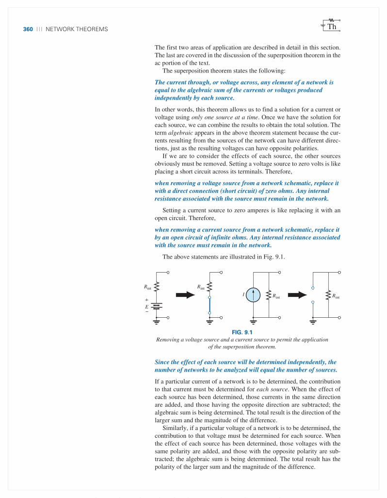
To expand on the above conclusion and further demonstrate what is meant by a nonlinear relationship, the power to the 6 Ω resistor versus current through the 6 Ω resistor is plotted in Fig. 9.6. Note that the curve is not a straight line but one whose rise gets steeper with increase in current level.
400
300
200
100
x
0 1 2 3 4 5 6 7 8 I6 (A( (
)))
P (W)
y
z
Nonlinear curve
(I ′2 I″2 IT)
FIG. 9.6Plotting power delivered to the 6 Ω resistor versus current
through the resistor.
Recall from Fig. 9.3 that the power level was 24 W for a cur-rent of 2 A developed by the 36 V voltage source, shown in Fig. 9.6. From Fig. 9.4, we found that the current level was 6 A for a power level of 216 W, shown in Fig. 9.6. Using the total current of 8 A, we find that the power level in 384 W, shown in Fig. 9.6. Quite clearly, the sum of power levels due to the 2 A and 6 A current levels does not equal that due to the 8 A level. That is,
x + y ≠ z
Now, the relationship between the voltage across a resistor and the current through a resistor is a linear (straight line) one, as shown in Fig. 9.7, with
c = a + b
4
3
2
1
012 24 36 48 V6 (V
(()
))
I (A)
a
c
Linear curveb
8
7
6
5
910
(I ′2 I″2 IT)
FIG. 9.7Plotting I versus V for the 6 Ω resistor.
GRIDLINE SET IN 1ST-PP TO INDICATE SAFE AREA; TO BE REMOVED AFTER 1ST-PP
M09_BOYL3605_13_SE_C09.indd Page 362 24/11/14 1:59 PM f403 /204/PH01893/9780133923605_BOYLESTAD/BOYLESTAD_INTRO_CIRCUIT_ANALYSIS13_SE_978013 ...

superpositioN theorem 363Th
EXAMPLE 9.2 Using the superposition theorem, determine the current through the 12 Ω resistor in Fig. 9.8. Note that this is a two-source net-work of the type examined in the previous chapter when we applied branch-current analysis and mesh analysis.
Solution: Considering the effects of the 54 V source requires replac-ing the 48 V source by a short-circuit equivalent as shown in Fig. 9.9. The result is that the 12 Ω and 4 Ω resistors are in parallel.
The total resistance seen by the source is therefore
RT = R1 + R2 R3 = 24 Ω + 12 Ω 4 Ω = 24 Ω + 3 Ω = 27 Ω
and the source current is
Is =E1
RT=
54 V
27 Ω= 2 A
R1
24
R3
4
E1 54 V
I2 = ?
R2 12 E2 48 V
FIG. 9.8Using the superposition theorem to determine the current through the 12 Ω resistor (Example 9.2).
48 V batteryreplaced by short
circuit
3
RT
IsR1
24
R3
4
E1 54 V E1 54 V
R1
24
R2 12 R2 12 R3 4
I2 I2
FIG. 9.9Using the superposition theorem to determine the effect of the 54 V voltage source on current I2 in Fig. 9.8.
Using the current divider rule results in the contribution to I2 due to the 54 V source:
I′2 =R3Is
R3 + R2=
(4 Ω)(2 A)
4 Ω + 12 Ω= 0.5 A
If we now replace the 54 V source by a short-circuit equivalent, the network in Fig. 9.10 results. The result is a parallel connection for the 12 Ω and 24 Ω resistors.
Therefore, the total resistance seen by the 48 V source is
RT = R3 + R2 R1 = 4 Ω + 12 Ω 24 Ω = 4 Ω + 8 Ω = 12 Ω
48 V
8
RT
E2
R1
24
R2 12
I2 I2
R3
4
E2 R2 12 R1 24 48 V
R3
4
54 V battery replacedby short circuit
FIG. 9.10Using the superposition theorem to determine the effect of the 48 V voltage source on current I2 in Fig. 9.8.
GRIDLINE SET IN 1ST-PP TO INDICATE SAFE AREA; TO BE REMOVED AFTER 1ST-PP
M09_BOYL3605_13_SE_C09.indd Page 363 24/11/14 1:59 PM f403 /204/PH01893/9780133923605_BOYLESTAD/BOYLESTAD_INTRO_CIRCUIT_ANALYSIS13_SE_978013 ...

364 Network theorems Th
and the source current is
Is =E2
RT=
48 V
12 Ω= 4 A
Applying the current divider rule results in
I″2 =R1(Is)
R1 + R2=
(24 Ω)(4 A)
24 Ω + 12 Ω= 2.67 A
It is now important to realize that current I2 due to each source has a different direction, as shown in Fig. 9.11. The net current therefore is the difference of the two and in the direction of the larger as follows:
I2 = I″2 - I′2 = 2.67 A - 0.5 A = 2.17 A
Using Figs. 9.9 and 9.10 in Example 9.2, we can determine the other currents of the network with little added effort. That is, we can deter-mine all the branch currents of the network, matching an application of the branch-current analysis or mesh analysis approach. In general, there-fore, not only can the superposition theorem provide a complete solution for the network, but it also reveals the effect of each source on the desired quantity.
EXAMPLE 9.3 Using the superposition theorem, determine current I1 for the network in Fig. 9.12.
Solution: Since two sources are present, there are two networks to be analyzed. First let us determine the effects of the voltage source by set-ting the current source to zero amperes as shown in Fig. 9.13. Note that the resulting current is defined as I′1 because it is the current through resistor R1 due to the voltage source only.
Due to the open circuit, resistor R1 is in series (and, in fact, in paral-lel) with the voltage source E. The voltage across the resistor is the ap-plied voltage, and current I′1 is determined by
I′1 =V1
R1=
E
R1=
30 V
6 Ω= 5 A
Now for the contribution due to the current source. Setting the voltage source to zero volts results in the network in Fig. 9.14, which presents us with an interesting situation. The current source has been replaced with a short-circuit equivalent that is directly across the current source and resistor R1. Since the source current takes the path of least resistance, it chooses the zero ohm path of the inserted short-circuit equivalent, and the current through R1 is zero amperes. This is clearly demonstrated by an application of the current divider rule as follows:
I″1 =RscI
Rsc + R1=
(0 Ω)I
0 Ω + 6 Ω= 0 A
Since I′1 and I″1 have the same defined direction in Figs. 9.13 and 9.14, the total current is defined by
I1 = I′1 + I″1 = 5 A + 0 A = 5 A
Although this has been an excellent introduction to the application of the superposition theorem, it should be immediately clear in Fig. 9.12 that the voltage source is in parallel with the current source and load
R2 12
I2 = 0.5 A
I2 = 2.67 A
R2 12
I2 = 2.17 A
FIG. 9.11Using the results of Figs. 9.9 and 9.10 to determine
current I2 for the network in Fig. 9.8.
I 3 A
I1
E 30 V R1 6
FIG. 9.12Two-source network to be analyzed using the
superposition theorem in Example 9.3.
I1
E 30 V R1 6
FIG. 9.13Determining the effect of the 30 V supply on the
current I1 in Fig. 9.12.
R1 6 I
I
I
3 A
I1
FIG. 9.14Determining the effect of the 3 A current source on
the current I1 in Fig. 9.12.
GRIDLINE SET IN 1ST-PP TO INDICATE SAFE AREA; TO BE REMOVED AFTER 1ST-PP
M09_BOYL3605_13_SE_C09.indd Page 364 24/11/14 1:59 PM f403 /204/PH01893/9780133923605_BOYLESTAD/BOYLESTAD_INTRO_CIRCUIT_ANALYSIS13_SE_978013 ...
superpositioN theorem 365Th
resistor R1, so the voltage across each must be 30 V. The result is that I1 must be determined solely by
I1 =V1
R1=
E
R1=
30 V
6 Ω= 5 A
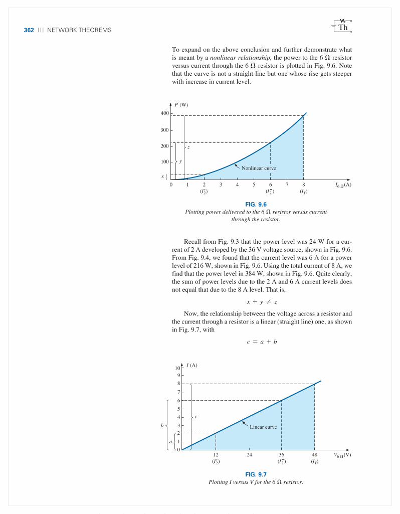
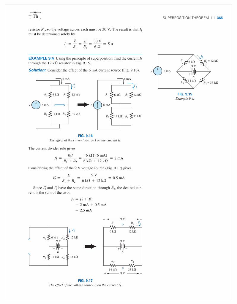
EXAMPLE 9.4 Using the principle of superposition, find the current I2 through the 12 kΩ resistor in Fig. 9.15.
Solution: Consider the effect of the 6 mA current source (Fig. 9.16).
R1 6 k
R314 k
R4 = 35 k
R2 = 12 k
6 mAI
I2
9 V
E+ –
FIG. 9.15Example 9.4.
R1 6 k
R3 14 k
R2 12 k
R4 35 k
6 mAI
I ′2
6 mA
6 mA
I ′2
I
R4 35 kR3 14 k
R2 12 kR1 6 k
6 mA
FIG. 9.16The effect of the current source I on the current I2.
The current divider rule gives
I′2 =R1I
R1 + R2=
(6 kΩ)(6 mA)
6 kΩ + 12 kΩ= 2 mA
Considering the effect of the 9 V voltage source (Fig. 9.17) gives
I″2 =E
R1 + R2=
9 V
6 kΩ + 12 kΩ= 0.5 mA
Since I′2 and I″2 have the same direction through R2, the desired cur-rent is the sum of the two:
I2 = I′2 + I″2 = 2 mA + 0.5 mA
= 2.5 mA
R1
6 k
R2
12 k
R3
14 k
R4
35 k
9 V
E
R1 6 k
R3 14 k
R2 12 k
R4 35 k
+ –9 V
+ –9 V
9 V
E
I2
I2
+ –+ –
FIG. 9.17The effect of the voltage source E on the current I2.
GRIDLINE SET IN 1ST-PP TO INDICATE SAFE AREA; TO BE REMOVED AFTER 1ST-PP
M09_BOYL3605_13_SE_C09.indd Page 365 24/11/14 1:59 PM f403 /204/PH01893/9780133923605_BOYLESTAD/BOYLESTAD_INTRO_CIRCUIT_ANALYSIS13_SE_978013 ...

366 Network theorems Th
EXAMPLE 9.5 Find the current through the 2 Ω resistor of the net-work in Fig. 9.18. The presence of three sources results in three different networks to be analyzed.
Solution: Consider the effect of the 12 V source (Fig. 9.19):
E1
R24
R1 2
I1
I 3 A
6 V12 V+ –
+
–E2
FIG. 9.18Example 9.5.
R24
R12
E1
12 V
I1I1
I1+ –
FIG. 9.19The effect of E1 on the current I.
R24 R12
6 V E2I1 I1
I 1
+
–
FIG. 9.20The effect of E2 on the current I1.
R24
R12 3 AI
I1
FIG. 9.21The effect of I on the current I1.
R1 2 R1 2 I1 = 2 A I 1 = 1 A I1 = 2 A I1 = 1 A
I1
FIG. 9.22The resultant current I1.
I′1 =E1
R1 + R2=
12 V
2 Ω + 4 Ω=
12 V
6 Ω= 2 A
Consider the effect of the 6 V source (Fig. 9.20):
I″1 =E2
R1 + R2=
6 V
2 Ω + 4 Ω=
6 V
6 Ω= 1 A
Consider the effect of the 3 A source (Fig. 9.21): Applying the current divider rule gives
I‴1 =R2I
R1 + R2=
(4 Ω)(3 A)
2 Ω + 4 Ω=
12 A
6= 2 A
The total current through the 2 Ω resistor appears in Fig. 9.22, and
I1 I I" I"1
' '
1 A 1 A2 A 2 A
Same directionas I1 in Fig. 9.18
Opposite directionto I1 in Fig. 9.18
1 1
9.3 THÉVENIN’S THEOREM
The next theorem to be introduced, Thévenin’s theorem, is probably one of the most interesting in that it permits the reduction of complex networks to a simpler form for analysis and design.
In general, the theorem can be used to do the following:
• Analyze networks with sources that are not in series or parallel.• Reduce the number of components required to establish the same
characteristics at the output terminals.
GRIDLINE SET IN 1ST-PP TO INDICATE SAFE AREA; TO BE REMOVED AFTER 1ST-PP
M09_BOYL3605_13_SE_C09.indd Page 366 24/11/14 1:59 PM f403 /204/PH01893/9780133923605_BOYLESTAD/BOYLESTAD_INTRO_CIRCUIT_ANALYSIS13_SE_978013 ...
théveNiN’s theorem 367Th
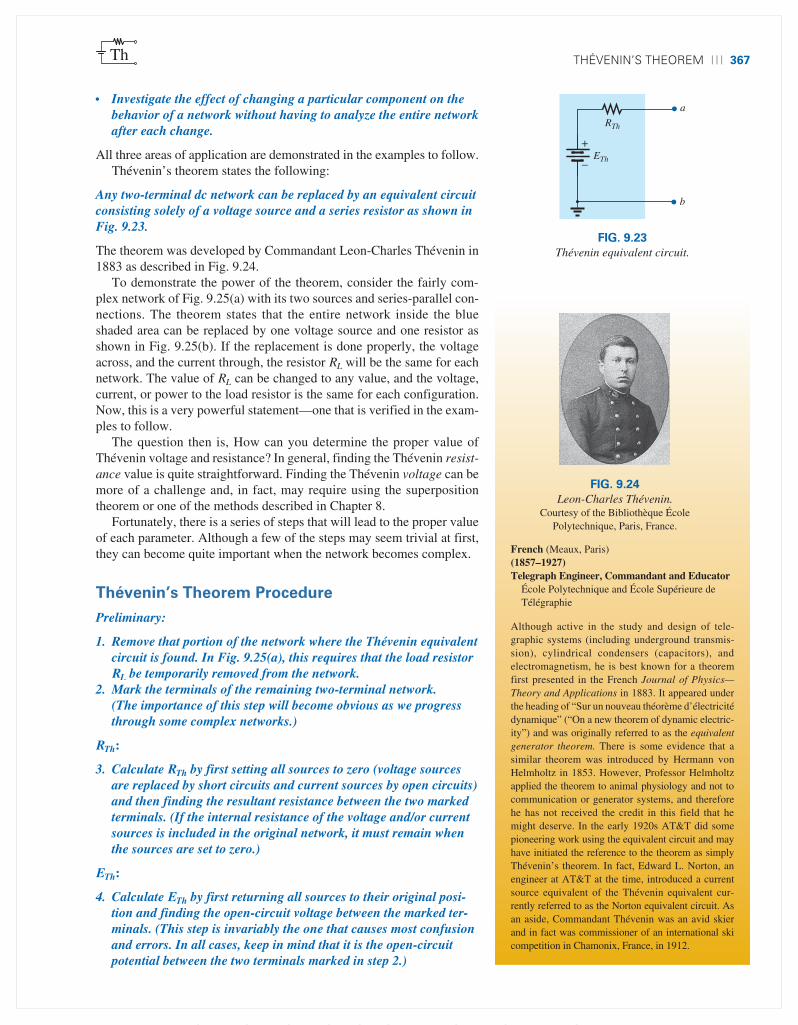
• Investigate the effect of changing a particular component on the behavior of a network without having to analyze the entire network after each change.
All three areas of application are demonstrated in the examples to follow.Thévenin’s theorem states the following:
Any two-terminal dc network can be replaced by an equivalent circuit consisting solely of a voltage source and a series resistor as shown in Fig. 9.23.
The theorem was developed by Commandant Leon-Charles Thévenin in 1883 as described in Fig. 9.24.
To demonstrate the power of the theorem, consider the fairly com-plex network of Fig. 9.25(a) with its two sources and series-parallel con-nections. The theorem states that the entire network inside the blue shaded area can be replaced by one voltage source and one resistor as shown in Fig. 9.25(b). If the replacement is done properly, the voltage across, and the current through, the resistor RL will be the same for each network. The value of RL can be changed to any value, and the voltage, current, or power to the load resistor is the same for each configuration. Now, this is a very powerful statement—one that is verified in the exam-ples to follow.
The question then is, How can you determine the proper value of Thévenin voltage and resistance? In general, finding the Thévenin resist-ance value is quite straightforward. Finding the Thévenin voltage can be more of a challenge and, in fact, may require using the superposition theorem or one of the methods described in Chapter 8.
Fortunately, there is a series of steps that will lead to the proper value of each parameter. Although a few of the steps may seem trivial at first, they can become quite important when the network becomes complex.
Thévenin’s Theorem Procedure
Preliminary:
1. Remove that portion of the network where the Thévenin equivalent circuit is found. In Fig. 9.25(a), this requires that the load resistor RL be temporarily removed from the network.
2. Mark the terminals of the remaining two-terminal network. (The importance of this step will become obvious as we progress through some complex networks.)
RTh:
3. Calculate RTh by first setting all sources to zero (voltage sources are replaced by short circuits and current sources by open circuits) and then finding the resultant resistance between the two marked terminals. (If the internal resistance of the voltage and/or current sources is included in the original network, it must remain when the sources are set to zero.)
ETh:
4. Calculate ETh by first returning all sources to their original posi-tion and finding the open-circuit voltage between the marked ter-minals. (This step is invariably the one that causes most confusion and errors. In all cases, keep in mind that it is the open-circuit potential between the two terminals marked in step 2.)
ETh
+
–
a
b
RTh
FIG. 9.23Thévenin equivalent circuit.
French (Meaux, Paris) (1857–1927)Telegraph Engineer, Commandant and Educator
École Polytechnique and École Supérieure de Télégraphie
Although active in the study and design of tele-graphic systems (including underground transmis-sion), cylindrical condensers (capacitors), and electromagnetism, he is best known for a theorem first presented in the French Journal of Physics—Theory and Applications in 1883. It appeared under the heading of “Sur un nouveau théorème d’électricité dynamique” (“On a new theorem of dynamic electric-ity”) and was originally referred to as the equivalent generator theorem. There is some evidence that a similar theorem was introduced by Hermann von Helmholtz in 1853. However, Professor Helmholtz applied the theorem to animal physiology and not to communication or generator systems, and therefore he has not received the credit in this field that he might deserve. In the early 1920s AT&T did some pioneering work using the equivalent circuit and may have initiated the reference to the theorem as simply Thévenin’s theorem. In fact, Edward L. Norton, an engineer at AT&T at the time, introduced a current source equivalent of the Thévenin equivalent cur-rently referred to as the Norton equivalent circuit. As an aside, Commandant Thévenin was an avid skier and in fact was commissioner of an international ski competition in Chamonix, France, in 1912.
FIG. 9.24Leon-Charles Thévenin.
Courtesy of the Bibliothèque École Polytechnique, Paris, France.
GRIDLINE SET IN 1ST-PP TO INDICATE SAFE AREA; TO BE REMOVED AFTER 1ST-PP
M09_BOYL3605_13_SE_C09.indd Page 367 24/11/14 1:59 PM f403 /204/PH01893/9780133923605_BOYLESTAD/BOYLESTAD_INTRO_CIRCUIT_ANALYSIS13_SE_978013 ...
368 Network theorems Th
Conclusion:
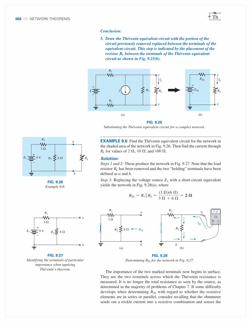
5. Draw the Thévenin equivalent circuit with the portion of the circuit previously removed replaced between the terminals of the equivalent circuit. This step is indicated by the placement of the resistor RL between the terminals of the Thévenin equivalent circuit as shown in Fig. 9.25(b).
R3
a
b
(a) (b)
E
a
IL
ETh
RTh
b
RLRL
IL
R1
R2
I
FIG. 9.25Substituting the Thévenin equivalent circuit for a complex network.
EXAMPLE 9.6 Find the Thévenin equivalent circuit for the network in the shaded area of the network in Fig. 9.26. Then find the current through RL for values of 2 Ω, 10 Ω, and 100 Ω.
Solution: Steps 1 and 2: These produce the network in Fig. 9.27. Note that the load resistor RL has been removed and the two “holding” terminals have been defined as a and b.
Step 3: Replacing the voltage source E1 with a short-circuit equivalent yields the network in Fig. 9.28(a), where
RTh = R1 R2 =(3 Ω)(6 Ω)
3 Ω + 6 Ω= 2
R1
3
R2 6
b
E1 9 V RL
a
+
–
FIG. 9.26Example 9.6.
R2 6
R1
3
E1 9 V
a
b
+
–
FIG. 9.27Identifying the terminals of particular
importance when applying Thévenin’s theorem.
+ –
R2 6
(a) (b)
R1
3
RThR2
b b
a a
I
R1
FIG. 9.28Determining RTh for the network in Fig. 9.27.
The importance of the two marked terminals now begins to surface. They are the two terminals across which the Thévenin resistance is measured. It is no longer the total resistance as seen by the source, as determined in the majority of problems of Chapter 7. If some difficulty develops when determining RTh with regard to whether the resistive elements are in series or parallel, consider recalling that the ohmmeter sends out a trickle current into a resistive combination and senses the
GRIDLINE SET IN 1ST-PP TO INDICATE SAFE AREA; TO BE REMOVED AFTER 1ST-PP
M09_BOYL3605_13_SE_C09.indd Page 368 24/11/14 1:59 PM f403 /204/PH01893/9780133923605_BOYLESTAD/BOYLESTAD_INTRO_CIRCUIT_ANALYSIS13_SE_978013 ...

théveNiN’s theorem 369Th
level of the resulting voltage to establish the measured resistance level. In Fig. 9.28(b), the trickle current of the ohmmeter approaches the net-work through terminal a, and when it reaches the junction of R1 and R2, it splits as shown. The fact that the trickle current splits and then recom-bines at the lower node reveals that the resistors are in parallel as far as the ohmmeter reading is concerned. In essence, the path of the sensing current of the ohmmeter has revealed how the resistors are connected to the two terminals of interest and how the Thévenin resistance should be determined. Remember this as you work through the various examples in this section.
Step 4: Replace the voltage source (Fig. 9.29). For this case, the open-circuit voltage ETh is the same as the voltage drop across the 6 Ω resistor. Applying the voltage divider rule gives
ETh =R2E1
R2 + R1=
(6 Ω)(9 V)
6 Ω + 3 Ω=
54 V
9= 6 V
It is particularly important to recognize that ETh is the open-circuit potential between points a and b. Remember that an open circuit can have any voltage across it, but the current must be zero. In fact, the cur-rent through any element in series with the open circuit must be zero also. The use of a voltmeter to measure ETh appears in Fig. 9.30. Note that it is placed directly across the resistor R2 since ETh and VR2
are in parallel.
Step 5: (Fig. 9.31):
IL =ETh
RTh + RL
RL = 2 Ω: IL =6 V
2 Ω + 2 Ω= 1.5 A
RL = 10 Ω: IL =6 V
2 Ω + 10 Ω= 0.5 A
RL = 100 Ω: IL =6 V
2 Ω + 100 Ω= 0.06 A
If Thévenin’s theorem were unavailable, each change in RL would require that the entire network in Fig. 9.26 be reexamined to find the new value of RL.
EXAMPLE 9.7 Find the Thévenin equivalent circuit for the network in the shaded area of the network in Fig. 9.32.
Solution:
Steps 1 and 2: See Fig. 9.33.
Step 3: See Fig. 9.34. The current source has been replaced with an open-circuit equivalent and the resistance determined between terminals a and b.
In this case, an ohmmeter connected between terminals a and b sends out a sensing current that flows directly through R1 and R2 (at the same level). The result is that R1 and R2 are in series and the Thévenin resist-ance is the sum of the two,
RTh = R1 + R2 = 4 Ω + 2 Ω = 6
R2 6 9 VE1 ETh
+
–
a
b
R1
3
+
–
+
–
FIG. 9.29Determining ETh for the network in Fig. 9.27.
+ –ETh
E1 R2 6
R1
3
9 V
+
–
+
–
FIG. 9.30Measuring ETh for the network in Fig. 9.27.
RL
aRTh = 2
ETh = 6 V
b
IL
+
–
FIG. 9.31Substituting the Thévenin equivalent circuit for the
network external to RL in Fig. 9.26.
R3 7
R2
2
R1 4
a
b
12 AI =
FIG. 9.32Example 9.7.
R2
2
R1 4 I12 A
a
b
FIG. 9.33Establishing the terminals of particular
interest for the network in Fig. 9.32.
GRIDLINE SET IN 1ST-PP TO INDICATE SAFE AREA; TO BE REMOVED AFTER 1ST-PP
M09_BOYL3605_13_SE_C09.indd Page 369 24/11/14 1:59 PM f403 /204/PH01893/9780133923605_BOYLESTAD/BOYLESTAD_INTRO_CIRCUIT_ANALYSIS13_SE_978013 ...

370 Network theorems Th
Step 4: See Fig. 9.35. In this case, since an open circuit exists between the two marked terminals, the current is zero between these terminals and through the 2 Ω resistor. The voltage drop across R2 is, therefore,
V2 = I2R2 = (0)R2 = 0 V
and ETh = V1 = I1R1 = IR1 = (12 A)(4 Ω) = 48 V
Step 5: See Fig. 9.36.
EXAMPLE 9.8 Find the Thévenin equivalent circuit for the network in the shaded area of the network in Fig. 9.37. Note in this example that there is no need for the section of the network to be preserved to be at the “end” of the configuration.
R1 4
a
b
RTh
R2
2
FIG. 9.34Determining RTh for the network
in Fig. 9.33.
R1 4
R2 = 2 I
I = 12 A
+
–
I = 0 +
–
+ V2 = 0 V – a
b
ETh
FIG. 9.35Determining ETh for the network
in Fig. 9.33.
R3 7
a
b
RTh = 6
ETh = 48 V+
–
FIG. 9.36Substituting the Thévenin equivalent circuit in the network external to the resistor R3 in Fig. 9.32.
8 VE1R4 3 R1 6
R2
4 a
b
+
–R3 2
FIG. 9.37Example 9.8.
Solution:
Steps 1 and 2: See Fig. 9.38.
R1 6
R2
4
R3 2 E1 8 V
a
b
–
+
FIG. 9.38Identifying the terminals of particular interest for the network in Fig. 9.37.
GRIDLINE SET IN 1ST-PP TO INDICATE SAFE AREA; TO BE REMOVED AFTER 1ST-PP
M09_BOYL3605_13_SE_C09.indd Page 370 24/11/14 1:59 PM f403 /204/PH01893/9780133923605_BOYLESTAD/BOYLESTAD_INTRO_CIRCUIT_ANALYSIS13_SE_978013 ...

théveNiN’s theorem 371Th
Step 3: See Fig. 9.39. Steps 1 and 2 are relatively easy to apply, but now we must be careful to “hold” onto the terminals a and b as the Thévenin resistance and voltage are determined. In Fig. 9.39, all the remaining elements turn out to be in parallel, and the network can be redrawn as shown. We have
RTh = R1 R2 =(6 Ω)(4 Ω)
6 Ω + 4 Ω=
24 Ω10
= 2.4
R2
4
R1 6 R2 4 R1 6
a
b
RTh
“Short circuited”
R3 2
Circuit redrawn:
RTh
a
b
RT = 0 2 = 0
FIG. 9.39Determining RTh for the network in Fig. 9.38.
ETh R1 6
R2
4
R3 2 ETh E1 8 V–
+
–
+
a
b +
–
FIG. 9.40Determining ETh for the network in Fig. 9.38.
R2 4
ETh R1 6
R3 2 –
+
–
+E1 8 V
FIG. 9.41Network of Fig. 9.40 redrawn.
Step 4: See Fig. 9.40. In this case, the network can be redrawn as shown in Fig. 9.41. Since the voltage is the same across parallel elements, the voltage across the series resistors R1 and R2 is E1, or 8 V. Applying the voltage divider rule gives
ETh =R1E1
R1 + R2=
(6 Ω)(8 V)
6 Ω + 4 Ω=
48 V
10= 4.8 V
Step 5: See Fig. 9.42.
The importance of marking the terminals should be obvious from Example 9.8. Note that there is no requirement that the Thévenin voltage have the same polarity as the equivalent circuit originally introduced.
R4 3
RTh = 2.4 a
b
ETh = 4.8 V–
+
FIG. 9.42Substituting the Thévenin equivalent circuit for the
network external to the resistor R4 in Fig. 9.37.
EXAMPLE 9.9 Find the Thévenin equivalent circuit for the network in the shaded area of the bridge network in Fig. 9.43.
R1
6 12
4
R2
RLR3 R4
3
b aE 72 V+
–
FIG. 9.43Example 9.9.
GRIDLINE SET IN 1ST-PP TO INDICATE SAFE AREA; TO BE REMOVED AFTER 1ST-PP
M09_BOYL3605_13_SE_C09.indd Page 371 24/11/14 1:59 PM f403 /204/PH01893/9780133923605_BOYLESTAD/BOYLESTAD_INTRO_CIRCUIT_ANALYSIS13_SE_978013 ...

372 Network theorems Th
Solution:
Steps 1 and 2: See Fig. 9.44.
Step 3: See Fig. 9.45. In this case, the short-circuit replacement of the volt-age source E provides a direct connection between c and c′ in Fig. 9.45(a), permitting a “folding” of the network around the horizontal line of a-b to produce the configuration in Fig. 9.45(b).
RTh = Ra - b = R1 R3 + R2 R4
= 6 Ω 3 Ω + 4 Ω 12 Ω = 2 Ω + 3 Ω = 5
R1
6
R2
12
4
R4R3
3
b a72 VE
+
–
FIG. 9.44Identifying the terminals of particular interest for the
network in Fig. 9.43.
R1
3 R1
6
R2
R3 R4
12
3 4
R2
R4
4
RTh
b a
R3
12 6
(b)(a)
abRTh
c′
c
c,c′
FIG. 9.45Solving for RTh for the network in Fig. 9.44.
Step 4: The circuit is redrawn in Fig. 9.46. The absence of a direct con-nection between a and b results in a network with three parallel branches. The voltages V1 and V2 can therefore be determined using the voltage divider rule:
V1 =R1E
R1 + R3=
(6 Ω)(72 V)
6 Ω + 3 Ω=
432 V
9= 48 V
V2 =R2E
R2 + R4=
(12 Ω)(72 V)
12 Ω + 4 Ω=
864 V
16= 54 V
V1 R1 6
R3 3
R2 12
R4 4
KVL+
–72 V
+
– +V2
b a
ETh–
+
E E–
+
–
FIG. 9.46Determining ETh for the network in Fig. 9.44.
RL
RTh = 5
ETh = 6 V
a
b
+
–
FIG. 9.47Substituting the Thévenin equivalent circuit for the
network external to the resistor RL in Fig. 9.43.
Assuming the polarity shown for ETh and applying Kirchhoff’s volt-age law to the top loop in the clockwise direction results in
gCV = + ETh + V1 - V2 = 0
and ETh = V2 - V1 = 54 V - 48 V = 6 V
Step 5: See Fig. 9.47.
GRIDLINE SET IN 1ST-PP TO INDICATE SAFE AREA; TO BE REMOVED AFTER 1ST-PP
M09_BOYL3605_13_SE_C09.indd Page 372 24/11/14 1:59 PM f403 /204/PH01893/9780133923605_BOYLESTAD/BOYLESTAD_INTRO_CIRCUIT_ANALYSIS13_SE_978013 ...

théveNiN’s theorem 373Th
Thévenin’s theorem is not restricted to a single passive element, as shown in the preceding examples, but can be applied across sources, whole branches, portions of networks, or any circuit configuration, as shown in the following example. It is also possible that you may have to use one of the methods previously described, such as mesh analysis or superposition, to find the Thévenin equivalent circuit.
EXAMPLE 9.10 (Two sources) Find the Thévenin circuit for the net-work within the shaded area of Fig. 9.48.
Solution:
Steps 1 and 2: See Fig. 9.49. The network is redrawn.
Step 3: See Fig. 9.50.
RTh = R4 + R1 R2 R3
= 1.4 kΩ + 0.8 kΩ 4 kΩ 6 kΩ = 1.4 kΩ + 0.8 kΩ 2.4 kΩ = 1.4 kΩ + 0.6 kΩ = 2 k
Step 4: Applying superposition, we will consider the effects of the volt-age source E1 first. Note Fig. 9.51. The open circuit requires that V4 = I4R4 = (0)R4 = 0 V, and
E′Th = V3
R′T = R2 R3 = 4 kΩ 6 kΩ = 2.4 kΩ
Applying the voltage divider rule gives
V3 =R′T E1
R′T + R1=
(2.4 kΩ)(6 V)
2.4 kΩ + 0.8 kΩ=
14.4 V
3.2= 4.5 V
E′Th = V3 = 4.5 V
For the source E2, the network in Fig. 9.52 results. Again, V4 =I4R4 = (0)R4 = 0 V, and
E″Th = V3
R′T = R1 R3 = 0.8 kΩ 6 kΩ = 0.706 kΩ
and
V3 =R″T E2
R″T + R2=
(0.706 kΩ)(10 V)
0.706 kΩ + 4 kΩ=
7.06 V
4.706= 1.5 V
E″Th = V3 = 1.5 V
R4
1.4 k
R3 6 k RLR1 0.8 k
R2 4 k
E2 + 10 V
E1 – 6 V
FIG. 9.48Example 9.10.
R1 0.8 k
R4
1.4 kR2 4 k
R3 6 k
E1 6 V E2 10 V+
–
–
+
a
b
FIG. 9.49Identifying the terminals of particular interest for
the network in Fig. 9.48.
2.4 k
R2 4 k
R3 6 k
R1 0.8 k
RTh
a
b
R4
1.4 k
FIG. 9.50Determining RTh for the network in Fig. 9.49.
R3 6 k
V4
1.4 k
E1
0.8 kR2 4 kR1
R4
6 V
I4 = 0
–
+
– +
V3
+
–ETh
+
–
FIG. 9.51Determining the contribution to ETh from the
source E1 for the network in Fig. 9.49.
R2 4 k
R3 6 k
E2 10 V
I4 = 0
EThV3
R4
1.4 k
V4+ –
+
–
+
–
R1 0.8 k+
–
FIG. 9.52Determining the contribution to ETh from the
source E2 for the network in Fig. 9.49.
GRIDLINE SET IN 1ST-PP TO INDICATE SAFE AREA; TO BE REMOVED AFTER 1ST-PP
M09_BOYL3605_13_SE_C09.indd Page 373 24/11/14 1:59 PM f403 /204/PH01893/9780133923605_BOYLESTAD/BOYLESTAD_INTRO_CIRCUIT_ANALYSIS13_SE_978013 ...
374 Network theorems Th
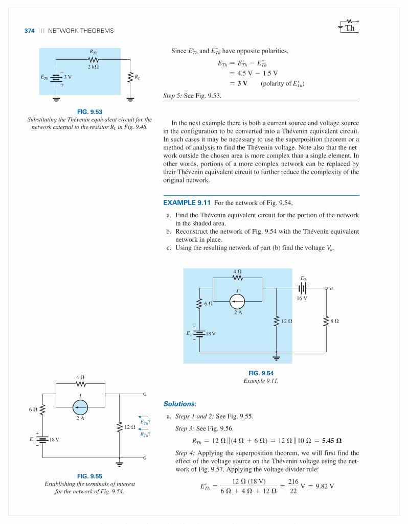
Since E′Th and E″Th have opposite polarities,
ETh = E′Th - E″Th
= 4.5 V - 1.5 V
= 3 V (polarity of E′Th)
Step 5: See Fig. 9.53.
RTh
2 k
RL3 VETh
+
–
FIG. 9.53Substituting the Thévenin equivalent circuit for the
network external to the resistor RL in Fig. 9.48.In the next example there is both a current source and voltage source
in the configuration to be converted into a Thévenin equivalent circuit. In such cases it may be necessary to use the superposition theorem or a method of analysis to find the Thévenin voltage. Note also that the net-work outside the chosen area is more complex than a single element. In other words, portions of a more complex network can be replaced by their Thévenin equivalent circuit to further reduce the complexity of the original network.
EXAMPLE 9.11 For the network of Fig. 9.54,
a. Find the Thévenin equivalent circuit for the portion of the network in the shaded area.
b. Reconstruct the network of Fig. 9.54 with the Thévenin equivalent network in place.
c. Using the resulting network of part (b) find the voltage Va.
4
6
8 12
E1
I
18 V
E2
16 V
a
2 A
FIG. 9.54Example 9.11.
Solutions:
a. Steps 1 and 2: See Fig. 9.55.
Step 3: See Fig. 9.56.
RTh = 12 Ω (4 Ω + 6 Ω) = 12 Ω 10 Ω = 5.45
Step 4: Applying the superposition theorem, we will first find the effect of the voltage source on the Thévenin voltage using the net-work of Fig. 9.57. Applying the voltage divider rule:
E′Th =12 Ω (18 V)
6 Ω + 4 Ω + 12 Ω=
216
22 V = 9.82 V
ETh?
RTh?
4
6
12
E1
I
18 V
2 A
FIG. 9.55Establishing the terminals of interest
for the network of Fig. 9.54.
GRIDLINE SET IN 1ST-PP TO INDICATE SAFE AREA; TO BE REMOVED AFTER 1ST-PP
M09_BOYL3605_13_SE_C09.indd Page 374 24/11/14 1:59 PM f403 /204/PH01893/9780133923605_BOYLESTAD/BOYLESTAD_INTRO_CIRCUIT_ANALYSIS13_SE_978013 ...

théveNiN’s theorem 375Th
The contribution due to the current source is determined using the network of Fig. 9.58(a) redrawn as shown in Fig. 9.58(b). Applying the current divider rule:
I′ =4 Ω (2 A)
4 Ω + 18 Ω=
8
22 A = 0.364 A
and E″Th = -I′(12 Ω) = -(0.364 A)(12 Ω) = -4.37 V
so that ETh = E′Th + E″Th = 9.82 V - 4.37 V = 5.45 V
b. The reconstructed network is shown in Fig. 9.59. c. Using the voltage divider rule:
Va =8 Ω (5.45 V + 16 V)
5.45 Ω + 8 Ω=
8 (21.45)
13.45 V =
171.6
13.45 V = 12.76 V
Instead of using the superposition theorem, the current source could first have been converted to a voltage source and the series elements com-bined to determine the Thévenin voltage. In any event both approaches would have yielded the same results.
Experimental Procedures
Now that the analytical procedure has been described in detail and a sense for the Thévenin impedance and voltage established, it is time to
4
6
12 RTh
FIG. 9.56Determining RTh.
4
6
12
18 VE1
–
+
ETh
FIG. 9.57Determining the contribution of E1 to ETh.
4
I
2 A
I 18
(b)(a)
6
I
12 ETh
+
–
4
I
2 A
FIG. 9.58Determining the contribution of I to ETh.
8
5.45
E2
16 V
5.45 V ETh
RThVa
Thévenin equivalent
FIG. 9.59Applying the Thévenin equivalent network to the
network of Fig. 9.54.
GRIDLINE SET IN 1ST-PP TO INDICATE SAFE AREA; TO BE REMOVED AFTER 1ST-PP
M09_BOYL3605_13_SE_C09.indd Page 375 24/11/14 1:59 PM f403 /204/PH01893/9780133923605_BOYLESTAD/BOYLESTAD_INTRO_CIRCUIT_ANALYSIS13_SE_978013 ...

376 Network theorems Th
investigate how both quantities can be determined using an experimental procedure.
Even though the Thévenin resistance is usually the easiest to deter-mine analytically, the Thévenin voltage is often the easiest to determine experimentally, and therefore it will be examined first.
Measuring ETh The network of Fig. 9.60(a) has the equivalent Thévenin circuit appearing in Fig. 9.60(b). The open-circuit Thévenin voltage can be determined by simply placing a voltmeter on the output terminals in Fig. 9.60(a) as shown. This is due to the fact that the open circuit in Fig. 9.60(b) dictates that the current through and the voltage across the Thévenin resistance must be zero. The result for Fig. 9.60(b) is that
Voc = ETh = 4.5 V
In general, therefore,
the Thévenin voltage is determined by connecting a voltmeter to the output terminals of the network. Be sure the internal resistance of the voltmeter is significantly more than the expected level of RTh.
4.50020V
V+ COM
4.50020V
V+ COM
4 I 8 A R1
12 V
R3 3
E
R2
1
Voc = ETh = 4.5 V
1.875
Voc = ETh = 4.5 V
V = 0 VRTh
4.5 VETh
I = 0 A
(a) (b)
FIG. 9.60Measuring the Thévenin voltage with a voltmeter: (a) actual network; (b) Thévenin equivalent.
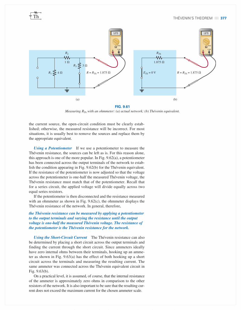
Measuring RTh
Using An Ohmmeter In Fig. 9.61, the sources in Fig. 9.60(a) have been set to zero, and an ohmmeter has been applied to measure the Thévenin resistance. In Fig. 9.60(b), it is clear that if the Thévenin voltage is set to zero volts, the ohmmeter will read the Thévenin resist-ance directly.
In general, therefore,
the Thévenin resistance can be measured by setting all the sources to zero and measuring the resistance at the output terminals.
It is important to remember, however, that ohmmeters cannot be used on live circuits, and you cannot set a voltage source by putting a short circuit across it—it causes instant damage. The source must either be set to zero or removed entirely and then replaced by a direct connection. For
GRIDLINE SET IN 1ST-PP TO INDICATE SAFE AREA; TO BE REMOVED AFTER 1ST-PP
M09_BOYL3605_13_SE_C09.indd Page 376 24/11/14 1:59 PM f403 /204/PH01893/9780133923605_BOYLESTAD/BOYLESTAD_INTRO_CIRCUIT_ANALYSIS13_SE_978013 ...
théveNiN’s theorem 377Th
the current source, the open-circuit condition must be clearly estab-lished; otherwise, the measured resistance will be incorrect. For most situations, it is usually best to remove the sources and replace them by the appropriate equivalent.
Using a Potentiometer If we use a potentiometer to measure the Thévenin resistance, the sources can be left as is. For this reason alone, this approach is one of the more popular. In Fig. 9.62(a), a potentiometer has been connected across the output terminals of the network to estab-lish the condition appearing in Fig. 9.62(b) for the Thévenin equivalent. If the resistance of the potentiometer is now adjusted so that the voltage across the potentiometer is one-half the measured Thévenin voltage, the Thévenin resistance must match that of the potentiometer. Recall that for a series circuit, the applied voltage will divide equally across two equal series resistors.
If the potentiometer is then disconnected and the resistance measured with an ohmmeter as shown in Fig. 9.62(c), the ohmmeter displays the Thévenin resistance of the network. In general, therefore,
the Thévenin resistance can be measured by applying a potentiometer to the output terminals and varying the resistance until the output voltage is one-half the measured Thévenin voltage. The resistance of the potentiometer is the Thévenin resistance for the network.
Using the Short-Circuit Current The Thévenin resistance can also be determined by placing a short circuit across the output terminals and finding the current through the short circuit. Since ammeters ideally have zero internal ohms between their terminals, hooking up an amme-ter as shown in Fig. 9.63(a) has the effect of both hooking up a short circuit across the terminals and measuring the resulting current. The same ammeter was connected across the Thévenin equivalent circuit in Fig. 9.63(b).
On a practical level, it is assumed, of course, that the internal resistance of the ammeter is approximately zero ohms in comparison to the other resistors of the network. It is also important to be sure that the resulting cur-rent does not exceed the maximum current for the chosen ammeter scale.
1.875
200Ω
COM+
1.875
200Ω
COM+
(a) (b)
1.875
R = RTh = 1.875
RTh
ETh = 0 V4 R1
R3 3
R2
1
R = RTh = 1.875
FIG. 9.61Measuring RTh with an ohmmeter: (a) actual network; (b) Thévenin equivalent.
GRIDLINE SET IN 1ST-PP TO INDICATE SAFE AREA; TO BE REMOVED AFTER 1ST-PP
M09_BOYL3605_13_SE_C09.indd Page 377 24/11/14 1:59 PM f403 /204/PH01893/9780133923605_BOYLESTAD/BOYLESTAD_INTRO_CIRCUIT_ANALYSIS13_SE_978013 ...

378 Network theorems Th
2.25020V
V+ COM
2.25020V
V+ COM
(a) (b)
1.875
= RTh = 1.875
RTh
4.5 VETh RL= 2.25 V
ETh24 I 8 A R1
12 V
R3 3
E
R2
1
ETh2
1.875
200Ω
COM+
(c)
FIG. 9.62Using a potentiometer to determine RTh: (a) actual network; (b) Thévenin equivalent; (c) measuring RTh.
2.400
20A
ACOM+
2.400
20A
ACOM+
4 I 8 A R1
12 V
R3 3
E
R2
1
Isc
1.875
RTh
4.5 V
(a) (b)
ETh Isc = = 2.4 AEThRTh
FIG. 9.63Determining RTh using the short-circuit current: (a) actual network; (b) Thévenin equivalent.
GRIDLINE SET IN 1ST-PP TO INDICATE SAFE AREA; TO BE REMOVED AFTER 1ST-PP
M09_BOYL3605_13_SE_C09.indd Page 378 24/11/14 1:59 PM f403 /204/PH01893/9780133923605_BOYLESTAD/BOYLESTAD_INTRO_CIRCUIT_ANALYSIS13_SE_978013 ...
NortoN’s theorem 379Th
In Fig. 9.63(b), since the short-circuit current is
Isc =ETh
RTh
the Thévenin resistance can be determined by
RTh =ETh
Isc
In general, therefore,
the Thévenin resistance can be determined by hooking up an ammeter across the output terminals to measure the short-circuit current and then using the open-circuit voltage to calculate the Thévenin resistance in the following manner:
RTh =Voc
Isc (9.1)
As a result, we have three ways to measure the Thévenin resistance of a configuration. Because of the concern about setting the sources to zero in the first procedure and the concern about current levels in the last, the second method is often chosen.
9.4 NORTON’S THEOREM
In Section 8.2, we learned that every voltage source with a series inter-nal resistance has a current source equivalent. The current source equiv-alent can be determined by Norton’s theorem (Fig. 9.64). It can also be found through the conversions of Section 8.2.
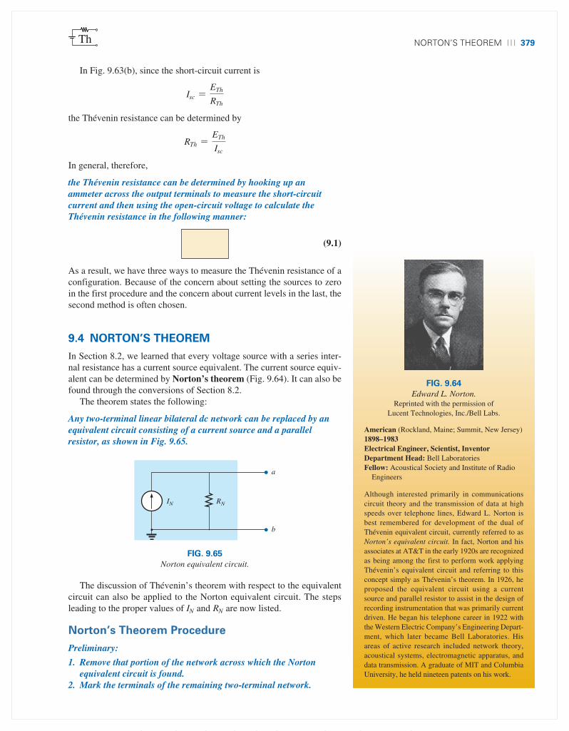
The theorem states the following:
Any two-terminal linear bilateral dc network can be replaced by an equivalent circuit consisting of a current source and a parallel resistor, as shown in Fig. 9.65.
American (Rockland, Maine; Summit, New Jersey) 1898–1983Electrical Engineer, Scientist, InventorDepartment Head: Bell LaboratoriesFellow: Acoustical Society and Institute of Radio
Engineers
Although interested primarily in communications circuit theory and the transmission of data at high speeds over telephone lines, Edward L. Norton is best remembered for development of the dual of Thévenin equivalent circuit, currently referred to as Norton’s equivalent circuit. In fact, Norton and his associates at AT&T in the early 1920s are recognized as being among the first to perform work applying Thévenin’s equivalent circuit and referring to this concept simply as Thévenin’s theorem. In 1926, he proposed the equivalent circuit using a current source and parallel resistor to assist in the design of recording instrumentation that was primarily current driven. He began his telephone career in 1922 with the Western Electric Company’s Engineering Depart-ment, which later became Bell Laboratories. His areas of active research included network theory, acoustical systems, electromagnetic apparatus, and data transmission. A graduate of MIT and Columbia University, he held nineteen patents on his work.
FIG. 9.64Edward L. Norton.
Reprinted with the permission of Lucent Technologies, Inc./Bell Labs.
RNIN
a
b
FIG. 9.65Norton equivalent circuit.
The discussion of Thévenin’s theorem with respect to the equivalent circuit can also be applied to the Norton equivalent circuit. The steps leading to the proper values of IN and RN are now listed.
Norton’s Theorem Procedure
Preliminary:
1. Remove that portion of the network across which the Norton equivalent circuit is found.
2. Mark the terminals of the remaining two-terminal network.
GRIDLINE SET IN 1ST-PP TO INDICATE SAFE AREA; TO BE REMOVED AFTER 1ST-PP
M09_BOYL3605_13_SE_C09.indd Page 379 24/11/14 1:59 PM f403 /204/PH01893/9780133923605_BOYLESTAD/BOYLESTAD_INTRO_CIRCUIT_ANALYSIS13_SE_978013 ...

380 Network theorems Th
RN:
3. Calculate RN by first setting all sources to zero (voltage sources are replaced with short circuits and current sources with open circuits) and then finding the resultant resistance between the two marked terminals. (If the internal resistance of the voltage and/or current sources is included in the original network, it must remain when the sources are set to zero.) Since RN = RTh, the procedure and value obtained using the approach described for Thévenin’s theorem will determine the proper value of RN.
IN:
4. Calculate IN by first returning all sources to their original posi-tion and then finding the short-circuit current between the marked terminals. It is the same current that would be measured by an ammeter placed between the marked terminals.
Conclusion:
5. Draw the Norton equivalent circuit with the portion of the circuit previously removed replaced between the terminals of the equivalent circuit.
The Norton and Thévenin equivalent circuits can also be found from each other by using the source transformation discussed earlier in this chapter and reproduced in Fig. 9.66.
RTh = RN
ETh
RThRN = RTh
ETh = IN RN
+
–IN
FIG. 9.66Converting between Thévenin and Norton equivalent circuits.
EXAMPLE 9.12 Find the Norton equivalent circuit for the network in the shaded area in Fig. 9.67.
Solution:
Steps 1 and 2: See Fig. 9.68.
Step 3: See Fig. 9.69, and
RN = R1 R2 = 3 Ω 6 Ω =(3 Ω)(6 Ω)
3 Ω + 6 Ω=
18 Ω9
= 2
Step 4: See Fig. 9.70, which clearly indicates that the short-circuit con-nection between terminals a and b is in parallel with R2 and eliminates its effect. IN is therefore the same as through R1, and the full battery volt-age appears across R1 since
V2 = I2R2 = (0)6 Ω = 0 V
Therefore,
IN =E
R1=
9 V
3 Ω= 3 A
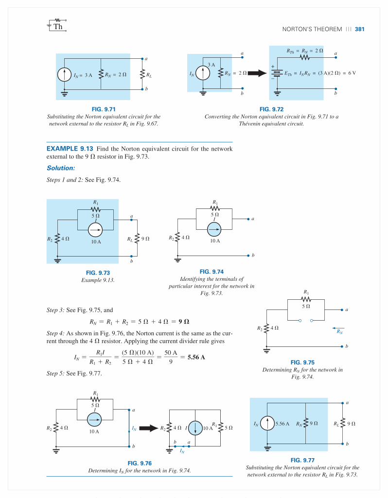
Step 5: See Fig. 9.71. This circuit is the same as the first one considered in the development of Thévenin’s theorem. A simple conversion indi-cates that the Thévenin circuits are, in fact, the same (Fig. 9.72).
R2 6
R1
3
RL9 VE+
–
a
b
FIG. 9.67Example 9.12.
R1
3
R2 6 9 V+
–
a
b
E
FIG. 9.68Identifying the terminals of particular interest for
the network in Fig. 9.67.
R2 6
R1
3
RN
a
b
FIG. 9.69Determining RN for the network in Fig. 9.68.
V2 R2 6
R1
3
Short circuited
E 9 V
Short
+
–
+
–
a
b
I1 IN IN
IN
I2 = 0
FIG. 9.70Determining IN for the network in Fig. 9.68.
GRIDLINE SET IN 1ST-PP TO INDICATE SAFE AREA; TO BE REMOVED AFTER 1ST-PP
M09_BOYL3605_13_SE_C09.indd Page 380 24/11/14 2:00 PM f403 /204/PH01893/9780133923605_BOYLESTAD/BOYLESTAD_INTRO_CIRCUIT_ANALYSIS13_SE_978013 ...
NortoN’s theorem 381Th
RLRN = 2 IN = 3 A
a
b
FIG. 9.71Substituting the Norton equivalent circuit for the network external to the resistor RL in Fig. 9.67.
RTh = RN = 2
IN RN = 2
3 A
a
b
ETh = IN RN = (3 A)(2 ) = 6 V
a
b
+
–
FIG. 9.72Converting the Norton equivalent circuit in Fig. 9.71 to a
Thévenin equivalent circuit.
EXAMPLE 9.13 Find the Norton equivalent circuit for the network external to the 9 Ω resistor in Fig. 9.73.
Solution:
Steps 1 and 2: See Fig. 9.74.
R1
5
10 A
a
b
RL 9 R2 4
I
FIG. 9.73Example 9.13.
R2 4
R1
5
10 A
a
b
I
FIG. 9.74Identifying the terminals of
particular interest for the network in Fig. 9.73.
R2 4
R1
5 a
b
RN
FIG. 9.75Determining RN for the network in
Fig. 9.74.
10 AR2 4
R1
5 a
b
INR1 5
b a
IR2 4
I
IN
10 A
FIG. 9.76Determining IN for the network in Fig. 9.74.
9 RL 9 IN 5.56 A
a
b
RN
FIG. 9.77Substituting the Norton equivalent circuit for the network external to the resistor RL in Fig. 9.73.
Step 3: See Fig. 9.75, and
RN = R1 + R2 = 5 Ω + 4 Ω = 9
Step 4: As shown in Fig. 9.76, the Norton current is the same as the cur-rent through the 4 Ω resistor. Applying the current divider rule gives
IN =R1I
R1 + R2=
(5 Ω)(10 A)
5 Ω + 4 Ω=
50 A
9= 5.56 A
Step 5: See Fig. 9.77.
GRIDLINE SET IN 1ST-PP TO INDICATE SAFE AREA; TO BE REMOVED AFTER 1ST-PP
M09_BOYL3605_13_SE_C09.indd Page 381 24/11/14 2:00 PM f403 /204/PH01893/9780133923605_BOYLESTAD/BOYLESTAD_INTRO_CIRCUIT_ANALYSIS13_SE_978013 ...

382 Network theorems Th
EXAMPLE 9.14 (Two sources) Find the Norton equivalent circuit for the portion of the network to the left of a-b in Fig. 9.78.
R3 9
R4 10 R2 6 R1 4
E1 7 V
I 8 A
E2 12 V
b
a
+
– +
–
FIG. 9.78Example 9.14.
IN 6.25 AR3 9
RN = 2.4
E2 12 V
R4 10
a
b
+
–
FIG. 9.83Substituting the Norton equivalent circuit for the network to the left of
terminals a@b in Fig. 9.78.
Solution:
Steps 1 and 2: See Fig. 9.79.
Step 3: See Fig. 9.80, and
RN = R1 R2 = 4 Ω 6 Ω =(4 Ω)(6 Ω)
4 Ω + 6 Ω=
24 Ω10
= 2.4
Step 4: (Using superposition) For the 7 V battery (Fig. 9.81),
I′N =E1
R1=
7 V
4 Ω= 1.75 A
For the 8 A source (Fig. 9.82), we find that both R1 and R2 have been “short circuited” by the direct connection between a and b, and
I″N = I = 8 A
The result is
IN = I″N - I′N = 8 A - 1.75 A = 6.25 A
Step 5: See Fig. 9.83.
R1 4 R2 6
E1 7 V
I 8 A
a
b
+
–
FIG. 9.79Identifying the terminals of particular interest
for the network in Fig. 9.78.
R1 4
R2 6
a
b
RN
FIG. 9.80Determining RN for the network in Fig. 9.79.
R2 6 R1 4
Short circuited
E1 7 V
a
b
IN
+
–
IN
IN
FIG. 9.81Determining the contribution to IN from the voltage
source E1.
R1 4
R2 6 I 8 A
I N
a
b
I N I N
I N
Short circuited
FIG. 9.82Determining the contribution to IN from the current
source I.
Experimental Procedure
The Norton current is measured in the same way as described for the short-circuit current (Isc) for the Thévenin network. Since the Norton and Thévenin resistances are the same, the same procedures can be fol-lowed as described for the Thévenin network.
GRIDLINE SET IN 1ST-PP TO INDICATE SAFE AREA; TO BE REMOVED AFTER 1ST-PP
M09_BOYL3605_13_SE_C09.indd Page 382 24/11/14 2:00 PM f403 /204/PH01893/9780133923605_BOYLESTAD/BOYLESTAD_INTRO_CIRCUIT_ANALYSIS13_SE_978013 ...
maximum power traNsfer theorem 383Th
9.5 MAXIMUM POWER TRANSFER THEOREM
When designing a circuit, it is often important to be able to answer one of the following questions:
What load should be applied to a system to ensure that the load is receiving maximum power from the system?
Conversely:
For a particular load, what conditions should be imposed on the source to ensure that it will deliver the maximum power available?
Even if a load cannot be set at the value that would result in maxi-mum power transfer, it is often helpful to have some idea of the value that will draw maximum power so that you can compare it to the load at hand. For instance, if a design calls for a load of 100 Ω, to ensure that the load receives maximum power, using a resistor of 1 Ω or 1 kΩ results in a power transfer that is much less than the maximum possible. However, using a load of 82 Ω or 120 Ω probably results in a fairly good level of power transfer.
Fortunately, the process of finding the load that will receive maxi-mum power from a particular system is quite straightforward due to the maximum power transfer theorem, which states the following:
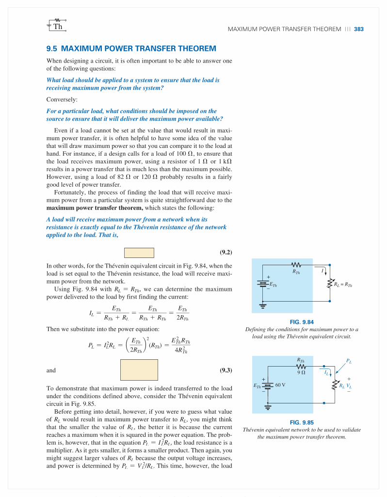
A load will receive maximum power from a network when its resistance is exactly equal to the Thévenin resistance of the network applied to the load. That is,
RL = RTh (9.2)
In other words, for the Thévenin equivalent circuit in Fig. 9.84, when the load is set equal to the Thévenin resistance, the load will receive maxi-mum power from the network.
Using Fig. 9.84 with RL = RTh, we can determine the maximum power delivered to the load by first finding the current:
IL =ETh
RTh + RL=
ETh
RTh + RTh=
ETh
2RTh
Then we substitute into the power equation:
PL = I2LRL = a ETh
2RThb
2
(RTh) =E 2
ThRTh
4R2Th
and PLmax=
E 2Th
4RTh (9.3)
To demonstrate that maximum power is indeed transferred to the load under the conditions defined above, consider the Thévenin equivalent circuit in Fig. 9.85.
Before getting into detail, however, if you were to guess what value of RL would result in maximum power transfer to RL, you might think that the smaller the value of RL, the better it is because the current reaches a maximum when it is squared in the power equation. The prob-lem is, however, that in the equation PL = I 2
LRL, the load resistance is a multiplier. As it gets smaller, it forms a smaller product. Then again, you might suggest larger values of RL because the output voltage increases, and power is determined by PL = V 2
L /RL. This time, however, the load
RL = RTh
IRTh
ETh
+
–
FIG. 9.84Defining the conditions for maximum power to a
load using the Thévenin equivalent circuit.
RL
IL
RTh
ETh
+
–
9
60 V VL
PL
+
–
FIG. 9.85Thévenin equivalent network to be used to validate
the maximum power transfer theorem.
GRIDLINE SET IN 1ST-PP TO INDICATE SAFE AREA; TO BE REMOVED AFTER 1ST-PP
M09_BOYL3605_13_SE_C09.indd Page 383 24/11/14 2:00 PM f403 /204/PH01893/9780133923605_BOYLESTAD/BOYLESTAD_INTRO_CIRCUIT_ANALYSIS13_SE_978013 ...

384 Network theorems Th
resistance is in the denominator of the equation and causes the resulting power to decrease. A balance must obviously be made between the load resistance and the resulting current or voltage. The following discussion shows that
maximum power transfer occurs when the load voltage and current are one-half their maximum possible values.
For the circuit in Fig. 9.85, the current through the load is determined by
IL =ETh
RTh + RL=
60 V
9 Ω + RL
The voltage is determined by
VL =RLETh
RL + RTh=
RL(60 V)
RL + RTh
and the power by
PL = I2LRL = a 60 V
9 Ω + RLb
2
(RL) =3600RL
(9 Ω + RL)2
If we tabulate the three quantities versus a range of values for RL from 0.1 Ω to 30 Ω, we obtain the results appearing in Table 9.1. Note in particular that when RL is equal to the Thévenin resistance of 9 Ω, the
TABLE 9.1
RL() PL(W) IL(A) VL(V)
0.1 4.35 6.60 0.660.2 8.51 6.52 1.300.5 19.94 6.32 3.161 36.00 6.00 6.002 59.50 5.46 10.913 75.00 5.00 15.004 85.21 4.62 18.465 91.84 4.29 21.436 96.00 4.00 24.007 98.44 Increase 3.75 Decrease 26.25 Increase8 99.65 3.53 28.239 (RTh) 100.00 (Maximum) 3.33 (Imax/2) 30.00 (ETh/2)
10 99.72 3.16 31.5811 99.00 3.00 33.0012 97.96 2.86 34.2913 96.69 2.73 35.4614 95.27 2.61 36.5215 93.75 2.50 37.5016 92.16 2.40 38.4017 90.53 2.31 39.2318 88.89 2.22 40.0019 87.24 2.14 40.7120 85.61 2.07 41.3825 77.86 1.77 44.1230 71.00 1.54 46.1540 59.98 1.22 48.98
100 30.30 0.55 55.05500 6.95 Decrease 0.12 Decrease 58.94 Increase
1000 3.54 0.06 59.47
GRIDLINE SET IN 1ST-PP TO INDICATE SAFE AREA; TO BE REMOVED AFTER 1ST-PP
M09_BOYL3605_13_SE_C09.indd Page 384 24/11/14 2:00 PM f403 /204/PH01893/9780133923605_BOYLESTAD/BOYLESTAD_INTRO_CIRCUIT_ANALYSIS13_SE_978013 ...

maximum power traNsfer theorem 385Th
power has a maximum value of 100 W, the current is 3.33 A, or one-half its maximum value of 6.67 A (as would result with a short circuit across the output terminals), and the voltage across the load is 30 V, or one-half its maximum value of 60 V (as would result with an open circuit across its output terminals). As you can see, there is no question that maximum power is transferred to the load when the load equals the Thévenin value.
The power to the load versus the range of resistor values is provided in Fig. 9.86. Note in particular that for values of load resistance less than the Thévenin value, the change is dramatic as it approaches the peak value. However, for values greater than the Thévenin value, the drop is a great deal more gradual. This is important because it tells us the following:
If the load applied is less than the Thévenin resistance, the power to the load will drop off rapidly as it gets smaller. However, if the applied load is greater than the Thévenin resistance, the power to the load will not drop off as rapidly as it increases.
For instance, the power to the load is at least 90 W for the range of about 4.5 Ω to 9 Ω below the peak value, but it is at least the same level for a range of about 9 Ω to 18 Ω above the peak value. The range below the peak is 4.5 Ω, while the range above the peak is almost twice as much at 9 Ω. As mentioned above, if maximum transfer conditions cannot be established, at least we now know from Fig. 9.86 that any resistance rela-tively close to the Thévenin value results in a strong transfer of power. More distant values such as 1 Ω or 100 Ω result in much lower levels.
It is particularly interesting to plot the power to the load versus load resistance using a log scale, as shown in Fig. 9.87. Logarithms will be discussed in detail in Chapter 22, but for now notice that the spacing
PL
PL (W)
0 5 9 10 15 20 25 30 RL ()
10
20
30
40
50
60
70
80
90
RL = RTh = 9
PLmax = 100
RTh
FIG. 9.86PL versus RL for the network in Fig. 9.85.
GRIDLINE SET IN 1ST-PP TO INDICATE SAFE AREA; TO BE REMOVED AFTER 1ST-PP
M09_BOYL3605_13_SE_C09.indd Page 385 24/11/14 2:00 PM f403 /204/PH01893/9780133923605_BOYLESTAD/BOYLESTAD_INTRO_CIRCUIT_ANALYSIS13_SE_978013 ...

386 Network theorems Th
between values of RL is not linear, but the distance, between powers of ten (such as 0.1 and 1, 1 and 10, and 10 and 100) are all equal. The advantage of the log scale is that a wide resistance range can be plotted on a relatively small graph.
Note in Fig. 9.87 that a smooth, bell-shaped curve results that is sym-metrical about the Thévenin resistance of 9 Ω. At 0.1 Ω, the power has dropped to about the same level as that at 1000 Ω, and at 1 Ω and 100 Ω, the power has dropped to the neighborhood of 30 W.
Although all of the above discussion centers on the power to the load, it is important to remember the following:
The total power delivered by a supply such as ETh is absorbed by both the Thévenin equivalent resistance and the load resistance. Any power delivered by the source that does not get to the load is lost to the Thévenin resistance.
Under maximum power conditions, only half the power delivered by the source gets to the load. Now, that sounds disastrous, but remember that we are starting out with a fixed Thévenin voltage and resistance, and the above simply tells us that we must make the two resistance levels equal if we want maximum power to the load. On an efficiency basis, we are working at only a 50% level, but we are content because we are getting maximum power out of our system.
The dc operating efficiency is defined as the ratio of the power deliv-ered to the load (PL) to the power delivered by the source (Ps). That is,
h% =PL
Ps* 100% (9.4)
For the situation where RL = RTh,
h% =I2
LRL
IL2RT
* 100% =RL
RT* 100% =
RTh
RTh + RTh* 100%
=RTh
2RTh* 100% =
1
2* 100% = 50%
Log scale
P (W)
100
90
80
70
60
50
40
30
20
10
0.1 0.5 1 2 3 4 5678 10 20 30 40 100 1000 RL ()
RL = RTh = 9
0.2
PL
PLmax
Linearscale
FIG. 9.87PL versus RL for the network in Fig. 9.85.
GRIDLINE SET IN 1ST-PP TO INDICATE SAFE AREA; TO BE REMOVED AFTER 1ST-PP
M09_BOYL3605_13_SE_C09.indd Page 386 24/11/14 2:00 PM f403 /204/PH01893/9780133923605_BOYLESTAD/BOYLESTAD_INTRO_CIRCUIT_ANALYSIS13_SE_978013 ...

maximum power traNsfer theorem 387Th
For the circuit in Fig. 9.85, if we plot the efficiency of operation ver-sus load resistance, we obtain the plot in Fig. 9.88, which clearly shows that the efficiency continues to rise to a 100% level as RL gets larger. Note in particular that the efficiency is 50% when RL = RTh.
To ensure that you completely understand the effect of the maximum power transfer theorem and the efficiency criteria, consider the circuit in Fig. 9.89, where the load resistance is set at 100 Ω and the power to the Thévenin resistance and to the load are calculated as follows:
IL =ETh
RTh + RL=
60 V
9 Ω + 100 Ω=
60 V
109 Ω= 550.5 mA
with PRTh= I2
LRTh = (550.5 mA)2(9 Ω) ≅ 2.73 W
and PL = I2LRL = (550.5 mA)2(100 Ω) ≅ 30.3 W
The results clearly show that most of the power supplied by the bat-tery is getting to the load—a desirable attribute on an efficiency basis. However, the power getting to the load is only 30.3 W compared to the 100 W obtained under maximum power conditions. In general, there-fore, the following guidelines apply:
If efficiency is the overriding factor, then the load should be much larger than the internal resistance of the supply. If maximum power transfer is desired and efficiency less of a concern, then the conditions dictated by the maximum power transfer theorem should be applied.
A relatively low efficiency of 50% can be tolerated in situations where power levels are relatively low, such as in a wide variety of electronic systems, where maximum power transfer for the given system is usually more important. However, when large power levels are involved, such as at generating plants, efficiencies of 50% cannot be tolerated. In fact, a great deal of expense and research is dedicated to raising power generat-ing and transmission efficiencies a few percentage points. Raising an effi-ciency level of a 10 MkW power plant from 94% to 95% (a 1% increase) can save 0.1 MkW, or 100 million watts, of power—an enormous saving.
100
75
50
25
0 20 40 60 80 100 RL ()
RL = RTh
%
10
η
≅ kRL 100%%η
Approaches 100%
FIG. 9.88Efficiency of operation versus increasing values of RL.
PE
PTh
PL
RL 100 ETh 60 V
RTh = 9
Power flow
FIG. 9.89Examining a circuit with high efficiency but a
relatively low level of power to the load.
GRIDLINE SET IN 1ST-PP TO INDICATE SAFE AREA; TO BE REMOVED AFTER 1ST-PP
M09_BOYL3605_13_SE_C09.indd Page 387 24/11/14 2:00 PM f403 /204/PH01893/9780133923605_BOYLESTAD/BOYLESTAD_INTRO_CIRCUIT_ANALYSIS13_SE_978013 ...

388 Network theorems Th
In all of the above discussions, the effect of changing the load was discussed for a fixed Thévenin resistance. Looking at the situation from a different viewpoint, we can say
if the load resistance is fixed and does not match the applied Thévenin equivalent resistance, then some effort should be made (if possible) to redesign the system so that the Thévenin equivalent resistance is closer to the fixed applied load.
In other words, if a designer faces a situation where the load resistance is fixed, he or she should investigate whether the supply section should be replaced or redesigned to create a closer match of resistance levels to produce higher levels of power to the load.
For the Norton equivalent circuit in Fig. 9.90, maximum power will be delivered to the load when
RL = RN (9.5)
This result [Eq. (9.5)] will be used to its fullest advantage in the analysis of transistor networks, where the most frequently applied transistor circuit model uses a current source rather than a voltage source.
For the Norton circuit in Fig. 9.90,
PLmax=
I2NRN
4 (W) (9.6)
EXAMPLE 9.15 A dc generator, battery, and laboratory supply are connected to resistive load RL in Fig. 9.91.
a. For each, determine the value of RL for maximum power transfer to RL. b. Under maximum power conditions, what are the current level and
the power to the load for each configuration? c. What is the efficiency of operation for each supply in part (b)? d. If a load of 1 kΩ were applied to the laboratory supply, what would
the power delivered to the load be? Compare your answer to the level of part (b). What is the level of efficiency?
e. For each supply, determine the value of RL for 75% efficiency.
RL = RN
I
RNIN
FIG. 9.90Defining the conditions for maximum power to a
load using the Norton equivalent circuit.
RL
2.5 Rint
–
+E
RL
0.05 Rint
E
RL
Rint
E
(a) dc generator (b) Battery (c) Laboratory supply
+
–
+
–
120 V
20
12 V 0–40 V
FIG. 9.91Example 9.15.
Solutions:
a. For the dc generator,
RL = RTh = Rint = 2.5
GRIDLINE SET IN 1ST-PP TO INDICATE SAFE AREA; TO BE REMOVED AFTER 1ST-PP
M09_BOYL3605_13_SE_C09.indd Page 388 24/11/14 2:00 PM f403 /204/PH01893/9780133923605_BOYLESTAD/BOYLESTAD_INTRO_CIRCUIT_ANALYSIS13_SE_978013 ...

maximum power traNsfer theorem 389Th
For the 12 V car battery,
RL = RTh = Rint = 0.05
For the dc laboratory supply,
RL = RTh = Rint = 20
b. For the dc generator,
PLmax=
E2Th
4RTh=
E2
4Rint=
(120 V)2
4(2.5 Ω)= 1.44 kW
For the 12 V car battery,
PLmax=
E2Th
4RTh=
E2
4Rint=
(12 V)2
4(0.05 Ω)= 720 W
For the dc laboratory supply,
PLmax=
E2Th
4RTh=
E2
4Rint=
(40 V)2
4(20 Ω)= 20 W
c. They are all operating under a 50% efficiency level because RL = RTh. d. The power to the load is determined as follows:
IL =E
Rint + RL=
40 V
20 Ω + 1000 Ω=
40 V
1020 Ω= 39.22 mA
and PL = I 2L RL = (39.22 mA)2(1000 Ω) = 1.54 W
The power level is significantly less than the 20 W achieved in part (b). The efficiency level is
h% =PL
Ps* 100% =
1.54 W
EIs* 100% =
1.54 W
(40 V)(39.22 mA)* 100%
=1.54 W
1.57 W* 100% = 98.09%
which is markedly higher than achieved under maximum power conditions—albeit at the expense of the power level.
e. For the dc generator,
h =Po
Ps=
RL
RTh + RL (h in decimal form)
and h =RL
RTh + RL
h(RTh + RL) = RL
hRTh + hRL = RL
RL(1 - h) = hRTh
and RL =hRTh
1 - h (9.7)
RL =0.75(2.5 Ω)
1 - 0.75= 7.5
For the battery,
RL =0.75(0.05 Ω)
1 - 0.75= 0.15
GRIDLINE SET IN 1ST-PP TO INDICATE SAFE AREA; TO BE REMOVED AFTER 1ST-PP
M09_BOYL3605_13_SE_C09.indd Page 389 24/11/14 2:00 PM f403 /204/PH01893/9780133923605_BOYLESTAD/BOYLESTAD_INTRO_CIRCUIT_ANALYSIS13_SE_978013 ...
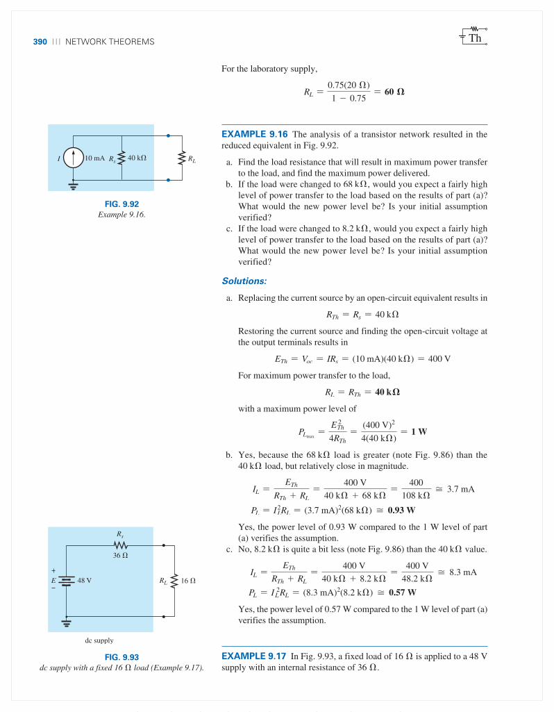
390 Network theorems Th
For the laboratory supply,
RL =0.75(20 Ω)
1 - 0.75= 60
EXAMPLE 9.16 The analysis of a transistor network resulted in the reduced equivalent in Fig. 9.92.
a. Find the load resistance that will result in maximum power transfer to the load, and find the maximum power delivered.
b. If the load were changed to 68 kΩ, would you expect a fairly high level of power transfer to the load based on the results of part (a)? What would the new power level be? Is your initial assumption verified?
c. If the load were changed to 8.2 kΩ, would you expect a fairly high level of power transfer to the load based on the results of part (a)? What would the new power level be? Is your initial assumption verified?
Solutions:
a. Replacing the current source by an open-circuit equivalent results in
RTh = Rs = 40 kΩ
Restoring the current source and finding the open-circuit voltage at the output terminals results in
ETh = Voc = IRs = (10 mA)(40 kΩ) = 400 V
For maximum power transfer to the load,
RL = RTh = 40 k
with a maximum power level of
PLmax=
E 2Th
4RTh=
(400 V)2
4(40 kΩ)= 1 W
b. Yes, because the 68 kΩ load is greater (note Fig. 9.86) than the 40 kΩ load, but relatively close in magnitude.
IL =ETh
RTh + RL=
400 V
40 kΩ + 68 kΩ=
400
108 kΩ≅ 3.7 mA
PL = I2LRL = (3.7 mA)2(68 kΩ) ≅ 0.93 W
Yes, the power level of 0.93 W compared to the 1 W level of part (a) verifies the assumption.
c. No, 8.2 kΩ is quite a bit less (note Fig. 9.86) than the 40 kΩ value.
IL =ETh
RTh + RL=
400 V
40 kΩ + 8.2 kΩ=
400 V
48.2 kΩ≅ 8.3 mA
PL = I 2L RL = (8.3 mA)2(8.2 kΩ) ≅ 0.57 W
Yes, the power level of 0.57 W compared to the 1 W level of part (a) verifies the assumption.
EXAMPLE 9.17 In Fig. 9.93, a fixed load of 16 Ω is applied to a 48 V supply with an internal resistance of 36 Ω.
I 10 mA Rs 40 k RL
FIG. 9.92Example 9.16.
dc supply
RL 16 48 V
36
Rs
E
FIG. 9.93dc supply with a fixed 16 Ω load (Example 9.17).
GRIDLINE SET IN 1ST-PP TO INDICATE SAFE AREA; TO BE REMOVED AFTER 1ST-PP
M09_BOYL3605_13_SE_C09.indd Page 390 24/11/14 2:00 PM f403 /204/PH01893/9780133923605_BOYLESTAD/BOYLESTAD_INTRO_CIRCUIT_ANALYSIS13_SE_978013 ...
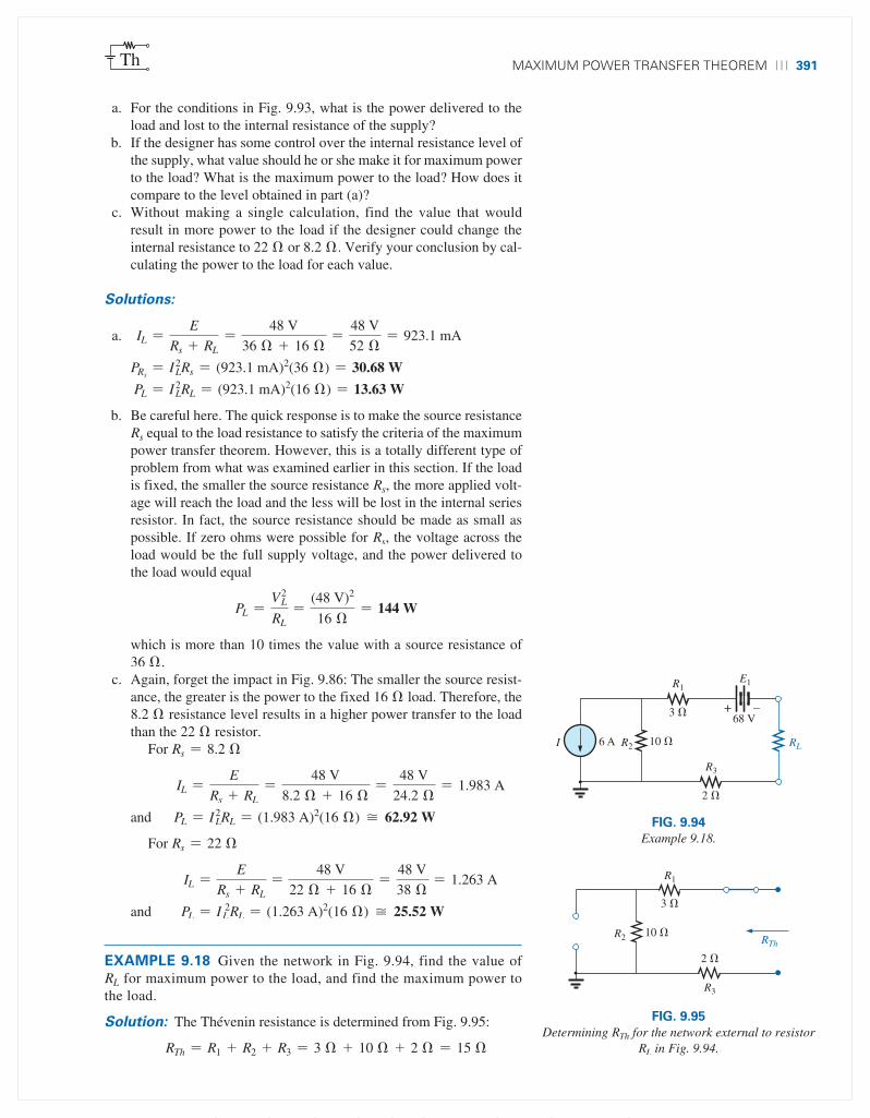
maximum power traNsfer theorem 391Th
a. For the conditions in Fig. 9.93, what is the power delivered to the load and lost to the internal resistance of the supply?
b. If the designer has some control over the internal resistance level of the supply, what value should he or she make it for maximum power to the load? What is the maximum power to the load? How does it compare to the level obtained in part (a)?
c. Without making a single calculation, find the value that would result in more power to the load if the designer could change the internal resistance to 22 Ω or 8.2 Ω. Verify your conclusion by cal-culating the power to the load for each value.
Solutions:
a. IL =E
Rs + RL=
48 V
36 Ω + 16 Ω=
48 V
52 Ω= 923.1 mA
PRs= I2
LRs = (923.1 mA)2(36 Ω) = 30.68 W
PL = I2LRL = (923.1 mA)2(16 Ω) = 13.63 W
b. Be careful here. The quick response is to make the source resistance Rs equal to the load resistance to satisfy the criteria of the maximum power transfer theorem. However, this is a totally different type of problem from what was examined earlier in this section. If the load is fixed, the smaller the source resistance Rs, the more applied volt-age will reach the load and the less will be lost in the internal series resistor. In fact, the source resistance should be made as small as possible. If zero ohms were possible for Rs, the voltage across the load would be the full supply voltage, and the power delivered to the load would equal
PL =V2
L
RL=
(48 V)2
16 Ω= 144 W
which is more than 10 times the value with a source resistance of 36 Ω.
c. Again, forget the impact in Fig. 9.86: The smaller the source resist-ance, the greater is the power to the fixed 16 Ω load. Therefore, the 8.2 Ω resistance level results in a higher power transfer to the load than the 22 Ω resistor.
For Rs = 8.2 Ω
IL =E
Rs + RL=
48 V
8.2 Ω + 16 Ω=
48 V
24.2 Ω= 1.983 A
and PL = I2LRL = (1.983 A)2(16 Ω) ≅ 62.92 W
For Rs = 22 Ω
IL =E
Rs + RL=
48 V
22 Ω + 16 Ω=
48 V
38 Ω= 1.263 A
and PL = I 2L RL = (1.263 A)2(16 Ω) ≅ 25.52 W
EXAMPLE 9.18 Given the network in Fig. 9.94, find the value of RL for maximum power to the load, and find the maximum power to the load.
Solution: The Thévenin resistance is determined from Fig. 9.95:
RTh = R1 + R2 + R3 = 3 Ω + 10 Ω + 2 Ω = 15 Ω
R2 10
R1
3
6 AI RL
E1
68 V
R3
2
+ –
FIG. 9.94Example 9.18.
R2 10
R1
3
R3
2
RTh
FIG. 9.95Determining RTh for the network external to resistor
RL in Fig. 9.94.
GRIDLINE SET IN 1ST-PP TO INDICATE SAFE AREA; TO BE REMOVED AFTER 1ST-PP
M09_BOYL3605_13_SE_C09.indd Page 391 24/11/14 2:00 PM f403 /204/PH01893/9780133923605_BOYLESTAD/BOYLESTAD_INTRO_CIRCUIT_ANALYSIS13_SE_978013 ...

392 Network theorems Th
so that RL = RTh = 15 Ω
The Thévenin voltage is determined using Fig. 9.96, where
V1 = V3 = 0 V and V2 = I2R2 = IR2 = (6 A)(10 Ω) = 60 V
Applying Kirchhoff’s voltage law gives
-V2 - E + ETh = 0
and ETh = V2 + E = 60 V + 68 V = 128 V
with the maximum power equal to
PLmax=
E2Th
4RTh=
(128 V)2
4(15 Ω)= 273.07 W
V2 R2 = 10
E1
68 VR1 = 3
I = 0
I = 6 AI = 0
R3 = 2 + V3 = 0 V –
ETh
–
+
– V1 = 0 V +
–
+6 A
I =
6 A
+ –
FIG. 9.96Determining ETh for the network external to resistor
RL in Fig. 9.94.
R1
E1
R2
E2
R3
E3
RL
Req
Eeq
RL
+
–
+
–
+
–
+
–
FIG. 9.97Demonstrating the effect of applying Millman’s theorem.
Step 1: Convert all voltage sources to current sources as outlined in Section 8.2. This is performed in Fig. 9.98 for the network in Fig. 9.97.
I1 E1G1 G1 I2 E2G2 I3G2 E3G3 G3 RL
( )E3R3
( )E2R2
( )E1R1
FIG. 9.98Converting all the sources in Fig. 9.97 to current sources.
9.6 MILLMAN’S THEOREM
Through the application of Millman’s theorem, any number of parallel voltage sources can be reduced to one. In Fig. 9.97, for example, the three voltage sources can be reduced to one. This permits finding the current through or voltage across RL without having to apply a method such as mesh analysis, nodal analysis, superposition, and so on. The theorem can best be described by applying it to the network in Fig. 9.97. Basically, three steps are included in its application.
GRIDLINE SET IN 1ST-PP TO INDICATE SAFE AREA; TO BE REMOVED AFTER 1ST-PP
M09_BOYL3605_13_SE_C09.indd Page 392 24/11/14 2:00 PM f403 /204/PH01893/9780133923605_BOYLESTAD/BOYLESTAD_INTRO_CIRCUIT_ANALYSIS13_SE_978013 ...

millmaN’s theorem 393Th
Step 2: Combine parallel current sources as described in Section 8.2. The resulting network is shown in Fig. 9.99, where
IT = I1 + I2 + I3 and GT = G1 + G2 + G3
Step 3: Convert the resulting current source to a voltage source, and the desired single-source network is obtained, as shown in Fig. 9.100.
In general, Millman’s theorem states that for any number of parallel voltage sources,
Eeq =IT
GT=
I1 I2 I3 g IN
G1 + G2 + G3 + g+ GN
or Eeq = E1G1 E2G2 E3G3 g ENGN
G1 + G2 + G3 + g+ GN (9.8)
The plus-and-minus signs appear in Eq. (9.8) to include those cases where the sources may not be supplying energy in the same direction. (Note Example 9.19.)
The equivalent resistance is
Req =1
GT=
1
G1 + G2 + G3 + g+ GN (9.9)
In terms of the resistance values,
Eeq =
E1
R1
E2
R2
E3
R3 g
EN
RN
1
R1+
1
R2+
1
R3+ g+
1
RN
(9.10)
and Req =1
1
R1+
1
R2+
1
R3+ g+
1
RN
(9.11)
Because of the relatively few direct steps required, you may find it easier to apply each step rather than memorizing and employing Eqs. (9.8) through (9.11).
EXAMPLE 9.19 Using Millman’s theorem, find the current through and voltage across the resistor RL in Fig. 9.101.
Solution: By Eq. (9.10),
Eeq =+
E1
R1-
E2
R2+
E3
R3
1
R1+
1
R2+
1
R3
The minus sign is used for E2>R2 because that supply has the opposite polarity of the other two. The chosen reference direction is therefore that of E1 and E3. The total conductance is unaffected by the direction, and
GTIT RL
FIG. 9.99Reducing all the current sources in Fig. 9.98 to a
single current source.
Req1
GT
EeqITGT
+
–
RL
FIG. 9.100Converting the current source in Fig. 9.99 to a
voltage source.
R1 5 R2 4 R3 2
E110 V
E216 V
E38 V
RL 3
IL
VL
+
–+
–
+
–+
–
FIG. 9.101Example 9.19.
GRIDLINE SET IN 1ST-PP TO INDICATE SAFE AREA; TO BE REMOVED AFTER 1ST-PP
M09_BOYL3605_13_SE_C09.indd Page 393 24/11/14 2:00 PM f403 /204/PH01893/9780133923605_BOYLESTAD/BOYLESTAD_INTRO_CIRCUIT_ANALYSIS13_SE_978013 ...
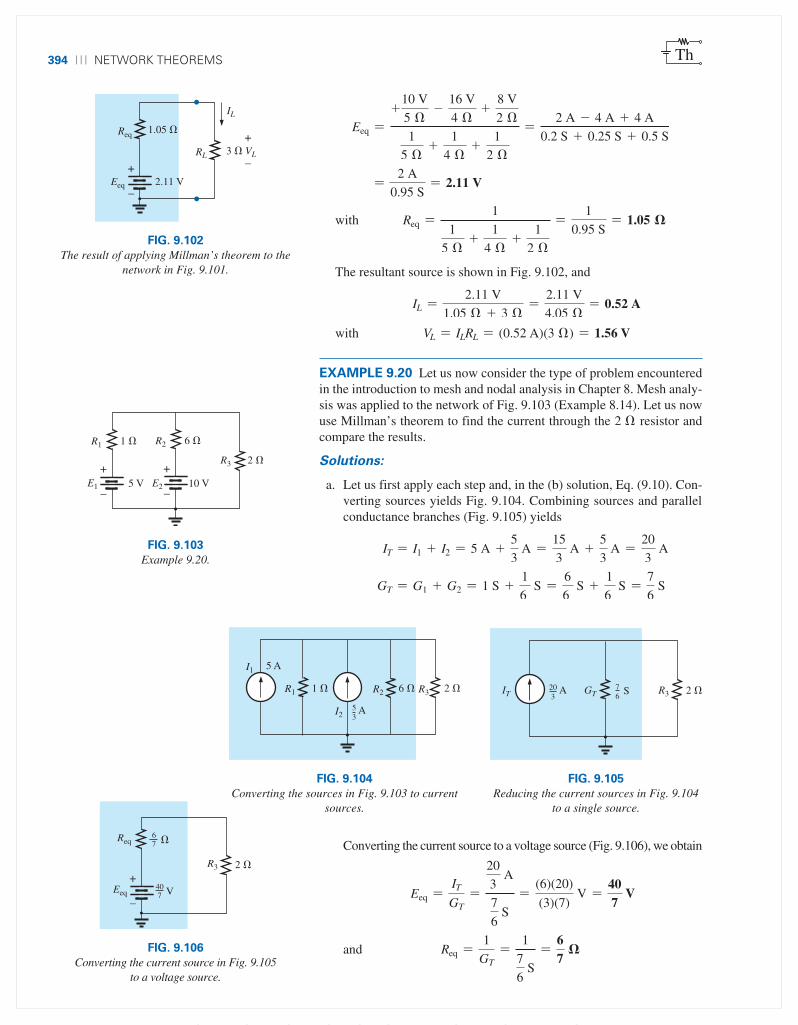
394 Network theorems Th
Eeq =+
10 V
5 Ω-
16 V
4 Ω+
8 V
2 Ω1
5 Ω+
1
4 Ω+
1
2 Ω
=2 A - 4 A + 4 A
0.2 S + 0.25 S + 0.5 S
=2 A
0.95 S= 2.11 V
with Req =1
1
5 Ω+
1
4 Ω+
1
2 Ω
=1
0.95 S= 1.05
The resultant source is shown in Fig. 9.102, and
IL =2.11 V
1.05 Ω + 3 Ω=
2.11 V
4.05 Ω= 0.52 A
with VL = ILRL = (0.52 A)(3 Ω) = 1.56 V
EXAMPLE 9.20 Let us now consider the type of problem encountered in the introduction to mesh and nodal analysis in Chapter 8. Mesh analy-sis was applied to the network of Fig. 9.103 (Example 8.14). Let us now use Millman’s theorem to find the current through the 2 Ω resistor and compare the results.
Solutions:
a. Let us first apply each step and, in the (b) solution, Eq. (9.10). Con-verting sources yields Fig. 9.104. Combining sources and parallel conductance branches (Fig. 9.105) yields
IT = I1 + I2 = 5 A +5
3 A =
15
3 A +
5
3 A =
20
3 A
GT = G1 + G2 = 1 S +1
6 S =
6
6 S +
1
6 S =
7
6 S
Req 1.05
Eeq
RL 3 VL–
+
2.11 V
IL
+
–
FIG. 9.102The result of applying Millman’s theorem to the
network in Fig. 9.101.
R1 1 R2 6
E1 5 V E2 10 V
R3 2 +
–
+
–
FIG. 9.103Example 9.20.
R3 2
67
Req
Eeq407 V
+
–
FIG. 9.106Converting the current source in Fig. 9.105
to a voltage source.
Converting the current source to a voltage source (Fig. 9.106), we obtain
Eeq =IT
GT=
20
3 A
7
6 S
=(6)(20)
(3)(7) V =
407
V
and Req =1
GT=
1
7
6 S
=67
IT203
76
R3 2 SA GT
FIG. 9.105Reducing the current sources in Fig. 9.104
to a single source.
I1
R1
5 A
1 R2 6
I253
R3 2
A
FIG. 9.104Converting the sources in Fig. 9.103 to current
sources.
GRIDLINE SET IN 1ST-PP TO INDICATE SAFE AREA; TO BE REMOVED AFTER 1ST-PP
M09_BOYL3605_13_SE_C09.indd Page 394 24/11/14 2:00 PM f403 /204/PH01893/9780133923605_BOYLESTAD/BOYLESTAD_INTRO_CIRCUIT_ANALYSIS13_SE_978013 ...

substitutioN theorem 395Th
so that
I2Ω =Eeq
Req + R3=
40
7 V
6
7 Ω + 2 Ω
=
40
7 V
6
7 Ω +
14
7 Ω
=40 V
20 Ω= 2 A
which agrees with the result obtained in Example 8.14. b. Let us now simply apply the proper equation, Eq. (9.10):
Eeq =+
5 V
1 Ω+
10 V
6 Ω1
1 Ω+
1
6 Ω
=
30 V
6 Ω+
10 V
6 Ω6
6 Ω+
1
6 Ω
=407
V
and
Req =1
1
1 Ω+
1
6 Ω
=1
6
6 Ω+
1
6 Ω
=1
7
6 S
=67
which are the same values obtained above.
The dual of Millman’s theorem (Fig. 9.97) appears in Fig. 9.107. It can be shown that Ieq and Req, as in Fig. 9.107, are given by
Ieq = I1R1 I2R2 I3R3
R1 + R2 + R3 (9.12)
and Req = R1 + R2 + R3 (9.13)
The derivation appears as a problem at the end of the chapter.
R1
I2
R2
I3
R3
I1
Req
Ieq
RL RL
FIG. 9.107The dual effect of Millman’s theorem.
9.7 SUBSTITUTION THEOREM
The substitution theorem states the following:
If the voltage across and the current through any branch of a dc bilateral network are known, this branch can be replaced by any combination of elements that will maintain the same voltage across and current through the chosen branch.
More simply, the theorem states that for branch equivalence, the terminal voltage and current must be the same. Consider the circuit in Fig. 9.108, in which the voltage across and current through the branch
R2 4
R1
6
a
b
3 A
E 30 V+
–12 V
+
–
FIG. 9.108Demonstrating the effect of the substitution theorem.
GRIDLINE SET IN 1ST-PP TO INDICATE SAFE AREA; TO BE REMOVED AFTER 1ST-PP
M09_BOYL3605_13_SE_C09.indd Page 395 24/11/14 2:00 PM f403 /204/PH01893/9780133923605_BOYLESTAD/BOYLESTAD_INTRO_CIRCUIT_ANALYSIS13_SE_978013 ...

396 Network theorems Th
a@b are determined. Through the use of the substitution theorem, a number of equivalent a@a′ branches are shown in Fig. 9.109.
Note that for each equivalent, the terminal voltage and current are the same. Also consider that the response of the remainder of the circuit in Fig. 9.108 is unchanged by substituting any one of the equivalent branches. As demonstrated by the single-source equivalents in Fig. 9.109, a known potential difference and current in a network can be replaced by an ideal voltage source and current source, respectively.
Understand that this theorem cannot be used to solve networks with two or more sources that are not in series or parallel. For it to be applied, a potential difference or current value must be known or found using one of the techniques discussed earlier. One application of the theorem is shown in Fig. 9.110. Note that in the figure the known potential differ-ence V was replaced by a voltage source, permitting the isolation of the portion of the network including R3, R4, and R5. Recall that this was basically the approach used in the analysis of the ladder network as we worked our way back toward the terminal resistance R5.
2 A 12 12 V
b
3 Aa
–
+
a
b–
+
2
6 V
3 A
12 V
a
b–
+
3 A 12 V
a
b
12 V
–
+3 A
+
–+
–
FIG. 9.109Equivalent branches for the branch a-b in Fig. 9.108.
R2
R3a
b
E V
–
+
R1
R4 R5
R3
b
E′ = V R5R4
a
+
–
+
–
FIG. 9.110Demonstrating the effect of knowing a voltage at some point in a complex network.
The current source equivalence of the above is shown in Fig. 9.111, where a known current is replaced by an ideal current source, permitting the isolation of R4 and R5.
R2 R4
R3
R5
ba
I
R5
a
I
b
R1
E+
–
R4
FIG. 9.111Demonstrating the effect of knowing a current at some point in a complex network.
GRIDLINE SET IN 1ST-PP TO INDICATE SAFE AREA; TO BE REMOVED AFTER 1ST-PP
M09_BOYL3605_13_SE_C09.indd Page 396 24/11/14 2:00 PM f403 /204/PH01893/9780133923605_BOYLESTAD/BOYLESTAD_INTRO_CIRCUIT_ANALYSIS13_SE_978013 ...

reciprocity theorem 397Th
Recall from the discussion of bridge networks that V = 0 and I = 0 were replaced by a short circuit and an open circuit, respectively. This substitution is a very specific application of the substitution theorem.
9.8 RECIPROCITY THEOREM
The reciprocity theorem is applicable only to single-source networks. It is, therefore, not a theorem used in the analysis of multisource net-works described thus far. The theorem states the following:
The current I in any branch of a network due to a single voltage source E anywhere else in the network will equal the current through the branch in which the source was originally located if the source is placed in the branch in which the current I was originally measured.
In other words, the location of the voltage source and the resulting current may be interchanged without a change in current. The theorem requires that the polarity of the voltage source have the same corre-spondence with the direction of the branch current in each position.
I
E
a
b
c
d
I
E
a
b
c
d
(a) (b)
+
–
+
–
FIG. 9.112Demonstrating the impact of the reciprocity theorem.
E 45 V
I
+
–
R3
2
R1
12
R2 6 R4 4
Is
FIG. 9.113Finding the current I due to a source E.
In the representative network in Fig. 9.112(a), the current I due to the voltage source E was determined. If the position of each is interchanged as shown in Fig. 9.112(b), the current I will be the same value as indi-cated. To demonstrate the validity of this statement and the theorem, consider the network in Fig. 9.113, in which values for the elements of Fig. 9.112(a) have been assigned.
The total resistance is
RT = R1 + R2 (R3 + R4) = 12 Ω + 6 Ω (2 Ω + 4 Ω)
= 12 Ω + 6 Ω 6 Ω = 12 Ω + 3 Ω = 15 Ω
and Is =E
RT=
45 V
15 Ω= 3 A
with I =3 A
2= 1.5 A
For the network in Fig. 9.114, which corresponds to that in Fig. 9.112(b), we find
RT = R4 + R3 + R1 R2
= 4 Ω + 2 Ω + 12 Ω 6 Ω = 10 Ω
and Is =E
RT=
45 V
10 Ω= 4.5 A
so that I =(6 Ω)(4.5 A)
12 Ω + 6 Ω=
4.5 A
3= 1.5 A
which agrees with the above.
R1
12
R3
2
R2 6 R4 4
E 45 V
I RT
Is
+
–
FIG. 9.114Interchanging the location of E and I of Fig. 9.113 to demonstrate the validity of the reciprocity theorem.
GRIDLINE SET IN 1ST-PP TO INDICATE SAFE AREA; TO BE REMOVED AFTER 1ST-PP
M09_BOYL3605_13_SE_C09.indd Page 397 24/11/14 2:01 PM f403 /204/PH01893/9780133923605_BOYLESTAD/BOYLESTAD_INTRO_CIRCUIT_ANALYSIS13_SE_978013 ...

398 Network theorems Th
The uniqueness and power of this theorem can best be demonstrated by considering a complex, single-source network such as the one shown in Fig. 9.115.
c
d
a
b
Ic
d
a
b
I
E
E+
–
+
–
FIG. 9.115Demonstrating the power and uniqueness of the reciprocity theorem.
9.9 COMPUTER ANALYSIS
Once you understand the mechanics of applying a software package or language, the opportunity to be creative and innovative presents itself. Through years of exposure and trial-and-error experiences, professional programmers develop a catalog of innovative techniques that are not only functional but very interesting and truly artistic in nature. Now that some of the basic operations associated with PSpice have been introduced, a few innovative maneuvers will be made in the examples to follow.
PSpice
Thévenin’s Theorem The application of Thévenin’s theorem requires an interesting maneuver to determine the Thévenin resistance. It is a maneuver, however, that has application beyond Thévenin’s theorem whenever a resistance level is required. The network to be analyzed appears in Fig. 9.116 and is the same one analyzed in Example 9.10 (Fig. 9.48).
Since PSpice is not set up to measure resistance levels directly, a 1 A current source can be applied as shown in Fig. 9.117, and Ohm’s law can be used to determine the magnitude of the Thévenin resistance in the following manner:
0RTh 0 = ` Vs
Is` = ` Vs
1 A` = 0Vs 0 (9.14)
In Eq. (9.14), since Is = 1A, the magnitude of RTh in ohms is the same as the magnitude of the voltage Vs (in volts) across the current source. The result is that when the voltage across the current source is displayed, it can be read as ohms rather than volts.
When PSpice is applied, the network appears as shown in Fig. 9.117. Flip the voltage source E1 and the current source by right-clicking on the source and choosing the Mirror Vertically option. Set both voltage sources to zero through the Display Properties dialog box obtained by double-clicking on the source symbol. The result of the Bias Point sim-ulation is 2 kV across the current source. The Thévenin resistance is therefore 2 kΩ between the two terminals of the network to the left of the current source (to match the results of Example 9.10). In total, by
R1 0.8 k
R4
1.4 k
R2 4 k
R3 6 k
+
–
E2 10 VE1 6 V–
+
ETh+
–
RTh
FIG. 9.116Network to which PSpice is to be applied to
determine ETh and RTh.
GRIDLINE SET IN 1ST-PP TO INDICATE SAFE AREA; TO BE REMOVED AFTER 1ST-PP
M09_BOYL3605_13_SE_C09.indd Page 398 24/11/14 2:01 PM f403 /204/PH01893/9780133923605_BOYLESTAD/BOYLESTAD_INTRO_CIRCUIT_ANALYSIS13_SE_978013 ...

computer aNalysis 399Th
setting the voltage source to 0 V, we have dictated that the voltage is the same at both ends of the voltage source, replicating the effect of a short-circuit connection between the two points.
For the open-circuit Thévenin voltage between the terminals of interest, the network must be constructed as shown in Fig. 9.118. The resistance of 1 T (= 1 million MΩ) is considered large enough to repre-sent an open circuit to permit an analysis of the network using PSpice. PSpice does not recognize floating nodes and generates an error signal if a connection is not made from the top right node to ground. Both voltage sources are now set on their prescribed values, and a simulation results in 3 V across the 1 T resistor. The open-circuit Thévenin voltage is therefore 3 V, which agrees with the solution in Example 9.10.
Maximum Power Transfer The procedure for plotting a quantity versus a parameter of the network is now introduced. In this case, the output power versus values of load resistance is used to verify that max-imum power is delivered to the load when its value equals the series Thévenin resistance. A number of new steps are introduced, but keep in mind that the method has broad application beyond Thévenin’s theorem and is therefore well worth the learning process.
The circuit to be analyzed appears in Fig. 9.119. The circuit is con-structed in exactly the same manner as described earlier except for the value of the load resistance. Begin the process by starting a New Project labeled PSpice 9-3, and build the circuit in Fig. 9.119. For the moment, do not set the value of the load resistance.
The first step is to establish the value of the load resistance as a vari-able since it will not be assigned a fixed value. Double-click on the value of RL, which is initially 1 kΩ, to obtain the Display Properties dialog
FIG. 9.117Using PSpice to determine the Thévenin resistance of a network through
the application of a 1 A current source.
GRIDLINE SET IN 1ST-PP TO INDICATE SAFE AREA; TO BE REMOVED AFTER 1ST-PP
M09_BOYL3605_13_SE_C09.indd Page 399 24/11/14 2:01 PM f403 /204/PH01893/9780133923605_BOYLESTAD/BOYLESTAD_INTRO_CIRCUIT_ANALYSIS13_SE_978013 ...
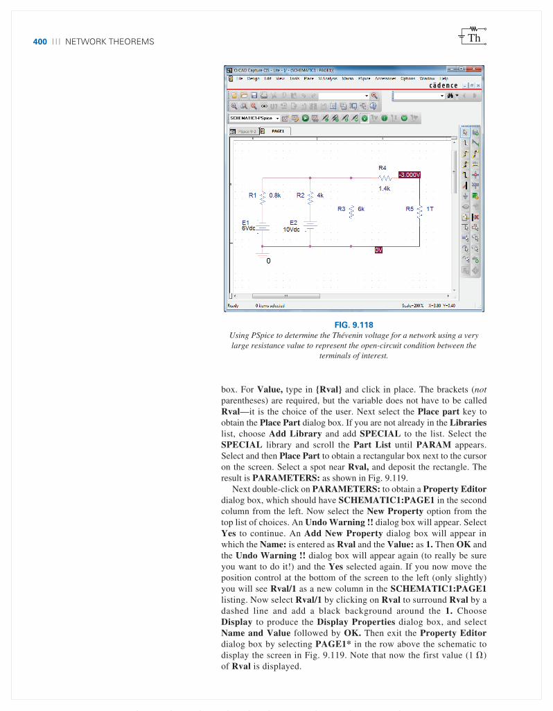
400 Network theorems Th
box. For Value, type in Rval and click in place. The brackets (not parentheses) are required, but the variable does not have to be called Rval—it is the choice of the user. Next select the Place part key to obtain the Place Part dialog box. If you are not already in the Libraries list, choose Add Library and add SPECIAL to the list. Select the SPECIAL library and scroll the Part List until PARAM appears. Select and then Place Part to obtain a rectangular box next to the cursor on the screen. Select a spot near Rval, and deposit the rectangle. The result is PARAMETERS: as shown in Fig. 9.119.
Next double-click on PARAMETERS: to obtain a Property Editor dialog box, which should have SCHEMATIC1:PAGE1 in the second column from the left. Now select the New Property option from the top list of choices. An Undo Warning !! dialog box will appear. Select Yes to continue. An Add New Property dialog box will appear in which the Name: is entered as Rval and the Value: as 1. Then OK and the Undo Warning !! dialog box will appear again (to really be sure you want to do it!) and the Yes selected again. If you now move the position control at the bottom of the screen to the left (only slightly) you will see Rval/1 as a new column in the SCHEMATIC1:PAGE1 listing. Now select Rval/1 by clicking on Rval to surround Rval by a dashed line and add a black background around the 1. Choose Display to produce the Display Properties dialog box, and select Name and Value followed by OK. Then exit the Property Editor dialog box by selecting PAGE1* in the row above the schematic to display the screen in Fig. 9.119. Note that now the first value (1 Ω) of Rval is displayed.
FIG. 9.118Using PSpice to determine the Thévenin voltage for a network using a very large resistance value to represent the open-circuit condition between the
terminals of interest.
GRIDLINE SET IN 1ST-PP TO INDICATE SAFE AREA; TO BE REMOVED AFTER 1ST-PP
M09_BOYL3605_13_SE_C09.indd Page 400 24/11/14 2:01 PM f403 /204/PH01893/9780133923605_BOYLESTAD/BOYLESTAD_INTRO_CIRCUIT_ANALYSIS13_SE_978013 ...

computer aNalysis 401Th
We are now ready to set up the simulation process. Select the New Simulation Profile key to open the New Simulation dialog box. Enter DC Sweep under Name followed by Create. A blinking Simulation Setting-Rval dialog box will then appear at the bottom of the screen that can be selected so it will appear in full size on the screen. After selecting Analysis, select DC Sweep under the Analysis type heading. Then leave the Primary Sweep under the Options heading, and select Global parameter under the Sweep variable. The Parameter name should then be entered as Rval. For the Sweep type, the Start value should be 1 Ω; but if we use 1 Ω, the curve to be generated will start at 1 Ω, leav-ing a blank from 0 to 1 Ω. The curve will look incomplete. To solve this problem, select 0.001 Ω as the Start value (very close to 0 Ω) with an Increment of 0.001 Ω. Enter the End value as 31 Ω to ensure a cal-culation at RL = 30.001 Ω. If we used 30 Ω as the end value, the last calculation would be at 29.001 Ω since 29.001 Ω + 1 Ω = 30.001 Ω, which is beyond the range of 30 Ω. The values of RL will therefore be 0.001 Ω, 1.001 Ω, 2.001 Ω, c29.001 Ω, 30.001 Ω, and so on, although the plot will look as if the values were 0 Ω, 1 Ω, 2 Ω, 29 Ω, 30 Ω, and so on. Click OK, and select the Run PSpice key, which will activate the analysis and result in a blinking yellow screen at the bottom of the win-dow. Select and the plot will appear as shown in Fig. 9.120.
Note that there are no plots on the graph, and that the graph extends to 40 Ω rather than 30 Ω as desired. It did not respond with a plot of power versus RL because we have not defined the plot of interest for the computer. To do this, select the Add Trace key (the key that has a red curve peaking in the middle of the plot) or Trace-Add Trace from the top menu bar. Either choice results in the Add Traces dialog box.
FIG. 9.119Using PSpice to plot the power to RL for a range of values for RL.
GRIDLINE SET IN 1ST-PP TO INDICATE SAFE AREA; TO BE REMOVED AFTER 1ST-PP
M09_BOYL3605_13_SE_C09.indd Page 401 24/11/14 2:01 PM f403 /204/PH01893/9780133923605_BOYLESTAD/BOYLESTAD_INTRO_CIRCUIT_ANALYSIS13_SE_978013 ...

402 Network theorems Th
The most important region of this dialog box is the Trace Expression listing at the bottom. The desired trace can be typed in directly, or the quantities of interest can be chosen from the list of Simulation Output Variables and deposited in the Trace Expression listing. To find the power to RL for the chosen range of values for RL, select W(RL) in the listing; it then appears as the Trace Expression. Click OK, and the plot in Fig. 9.121 appears. Originally, the plot extended from 0 Ω to 40 Ω. We reduced the range to 0 Ω to 31 Ω by selecting Plot-Axis Settings-X Axis-User Defined 0 to 31-OK.
Select the Toggle cursor key (which has an arrow set in a blue back-ground) at the top of the dialog box and seven options will open to the right of the key that include Cursor Peak, Cursor Trough, Cursor Slope, Cursor Min, Cursor Max, Cursor Point, and Cursor Search. Select Cursor Max (the fifth one over), and the Probe Cursor dialog box on the screen will reveal where the peak occurred and the power
FIG. 9.120Plot resulting from the dc sweep of RL for the network in Fig. 9.119 before
defining the parameters to be displayed.
FIG. 9.121A plot of the power delivered to RL in Fig. 9.119 for a range of values for RL
extending from 0 Ω to 30 Ω.
GRIDLINE SET IN 1ST-PP TO INDICATE SAFE AREA; TO BE REMOVED AFTER 1ST-PP
M09_BOYL3605_13_SE_C09.indd Page 402 24/11/14 2:01 PM f403 /204/PH01893/9780133923605_BOYLESTAD/BOYLESTAD_INTRO_CIRCUIT_ANALYSIS13_SE_978013 ...

computer aNalysis 403Th
level at that point. In the Probe Cursor dialog box the first column titled Trace Color reveals the color of the trace on the W(RL) plot. This becomes important when there is more than one trace on the screen. The next column titled Trace Name is labeled X values and gives the loca-tion on the horizontal axis for the point of interest Y1. Note that it is approximately 9 Ω to match the point of maximum power to the load RL. The next line reveals that the power W(RL) is 100W at RL = 9 Ω. There are other options available in the Probe Cursor dialog box by scrolling to the right.
It is possible that the Probe Cursor box will not appear as a separate entity on the screen but simply as an attachment at the bottom of the response screen. It can be isolated by deleting the dialog boxes to the right and left and then right-clicking the Toggle Cursor key. By simply unchecking the Allow Docking option the Probe Cursor dialog box will appear as a separate entity as obtained above. It can then be moved to any location on the screen. A second cursor can be generated by right-clicking the mouse on the Cursor Point option and moving it to a resist-ance of 30 Ω. The result is a power level of 71.009 W, as shown on the plot. Notice also that the plot generated appears as a listing at the bottom left of the screen as W(RL).
Multisim
Superposition Let us now apply superposition to the network in Fig. 9.122, which appeared earlier as Fig. 9.2 in Example 9.1, to permit a comparison of resulting solutions. The current through R2 is to be determined. With the use of methods described in earlier chapters for the application of Multisim, the network in Fig. 9.123 results, which
R2 6
R1
12 I2
I 9 AE 36 V+
–
FIG. 9.122Applying Multisim to determine the current I2 using
superposition.
FIG. 9.123Using Multisim to determine the contribution of the 36 V voltage source to the
current through R2.
GRIDLINE SET IN 1ST-PP TO INDICATE SAFE AREA; TO BE REMOVED AFTER 1ST-PP
M09_BOYL3605_13_SE_C09.indd Page 403 24/11/14 2:01 PM f403 /204/PH01893/9780133923605_BOYLESTAD/BOYLESTAD_INTRO_CIRCUIT_ANALYSIS13_SE_978013 ...
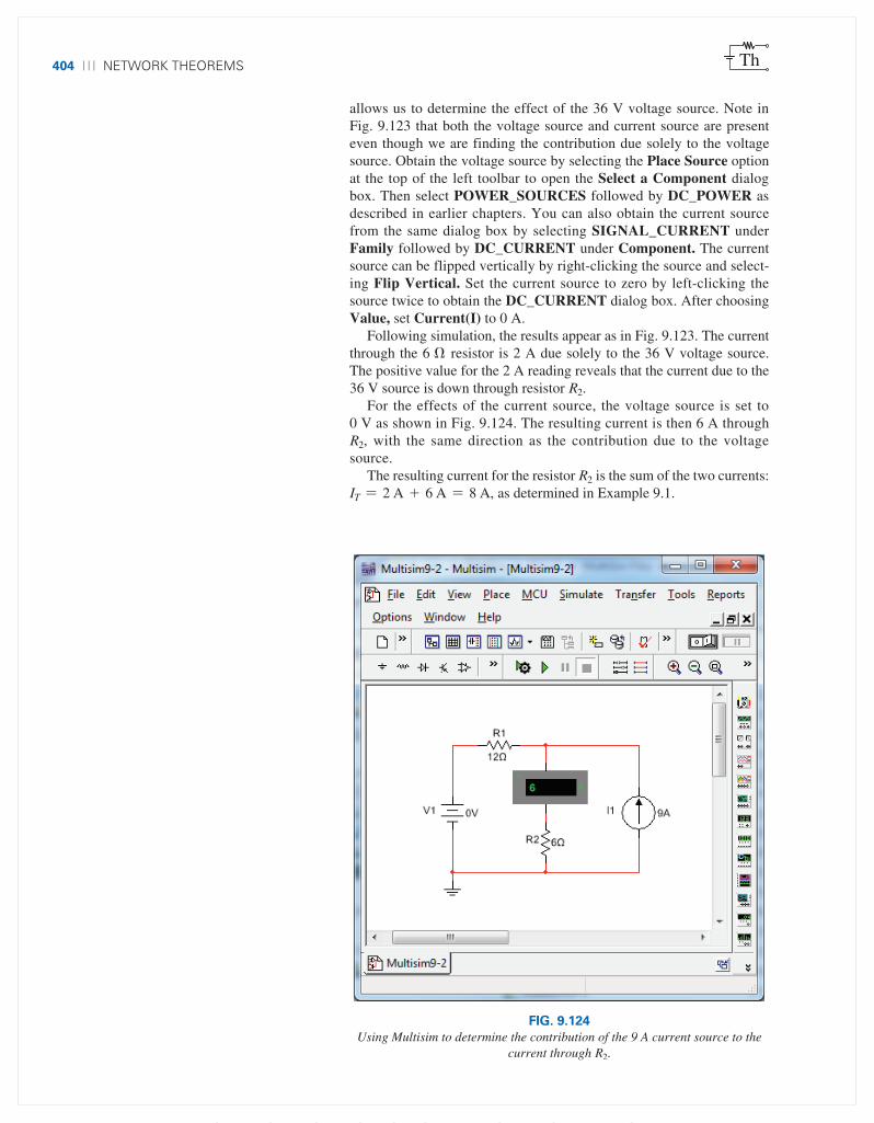
404 Network theorems Th
allows us to determine the effect of the 36 V voltage source. Note in Fig. 9.123 that both the voltage source and current source are present even though we are finding the contribution due solely to the voltage source. Obtain the voltage source by selecting the Place Source option at the top of the left toolbar to open the Select a Component dialog box. Then select POWER_SOURCES followed by DC_POWER as described in earlier chapters. You can also obtain the current source from the same dialog box by selecting SIGNAL_CURRENT under Family followed by DC_CURRENT under Component. The current source can be flipped vertically by right-clicking the source and select-ing Flip Vertical. Set the current source to zero by left-clicking the source twice to obtain the DC_CURRENT dialog box. After choosing Value, set Current(I) to 0 A.
Following simulation, the results appear as in Fig. 9.123. The current through the 6 Ω resistor is 2 A due solely to the 36 V voltage source. The positive value for the 2 A reading reveals that the current due to the 36 V source is down through resistor R2.
For the effects of the current source, the voltage source is set to 0 V as shown in Fig. 9.124. The resulting current is then 6 A through R2, with the same direction as the contribution due to the voltage source.
The resulting current for the resistor R2 is the sum of the two currents: IT = 2 A + 6 A = 8 A, as determined in Example 9.1.
FIG. 9.124Using Multisim to determine the contribution of the 9 A current source to the
current through R2.
GRIDLINE SET IN 1ST-PP TO INDICATE SAFE AREA; TO BE REMOVED AFTER 1ST-PP
M09_BOYL3605_13_SE_C09.indd Page 404 24/11/14 2:01 PM f403 /204/PH01893/9780133923605_BOYLESTAD/BOYLESTAD_INTRO_CIRCUIT_ANALYSIS13_SE_978013 ...

problems 405Th
PROBLEMS
SECTION 9.2 Superposition Theorem
1. a. Using the superposition theorem, determine the current through the 12 Ω resistor of Fig. 9.125.
b. Convert both voltage sources to current sources and recalculate the current to the 12 Ω resistor.
c. How do the results of parts (a) and (b) compare?
2. a. Using the superposition theorem, determine the voltage across the 4.7 Ω resistor of Fig. 9.126.
b. Find the power delivered to the 4.7 Ω resistor due solely to the current source.
c. Find the power delivered to the 4.7 Ω resistor due solely to the voltage source.
d. Find the power delivered to the 4.7 Ω resistor using the voltage found in part (a).
e. How do the results of part (d) compare with the sum of the results to parts (b) and (c)? Can the superposition theorem be applied to power levels?
R2
R3
I
10 VE2
R1
16 VE1
4 2
12
+
–+
–
FIG. 9.125Problem 1.
4.7
R2
3.3 12 V
E
2.4 R1 R33 AI
V
+–
+
–
FIG. 9.126Problem 2.
3. Using the superposition theorem, determine the current through the 56 Ω resistor of Fig. 9.127.
24 8 A
24 V 12 56 I
FIG. 9.127Problem 3.
4. Using superposition, find the current I through the 24 V source in Fig. 9.128.
R1 18
R2 9 R3 15 R4 10
24 V
E2
E1 = + 42 V
+– I
FIG. 9.128Problem 4.
5. Using superposition, find the voltage VR3 for the network of
Fig. 9.129.
10 k 18 kR1 R24 mA
18 V+–
R4
R3
4.7 k
3.3 k
VR3–+
FIG. 9.129Problem 5.
6. Using superposition, find the voltage V2 for the network in Fig. 9.130.
R1 12 k
I 9 mA
36 VE
V2
+
–R2
6.8 k
FIG. 9.130Problem 6.
GRIDLINE SET IN 1ST-PP TO INDICATE SAFE AREA; TO BE REMOVED AFTER 1ST-PP
M09_BOYL3605_13_SE_C09.indd Page 405 24/11/14 2:01 PM f403 /204/PH01893/9780133923605_BOYLESTAD/BOYLESTAD_INTRO_CIRCUIT_ANALYSIS13_SE_978013 ...

406 Network theorems Th
10. a. Find the Thévenin equivalent circuit for the network external to the resistor R for the network in Fig. 9.134.
b. Find the power delivered to R when R is 2 kΩ and 100 kΩ.
*8. Using superposition, find the voltage across the 6 A source in Fig. 9.132.
*7. Using superposition, find the current through R1 for the net-work in Fig. 9.131.
R2
3.3 k
R1 2.2 k
5 mA
2 mAI R4
R3
4.7 k
1.2 k
8 V
I1
+
–
FIG. 9.131Problem 7.
I = 6 A
R4 12
E2E1R2R1
4 + 8 V 12 V 6
R5
4 Vs+ –
–
FIG. 9.132Problem 8.
SECTION 9.3 Thévenin’s Theorem
9. a. Find the Thévenin equivalent circuit for the network external to the resistor R in Fig. 9.133.
b. Find the current through R when R is 2 Ω, 30 Ω, and 100 Ω.
R1
6
R2 3 E R18 V
R3
4
+
–
FIG. 9.133Problem 9.
R1.2 k
3.3 k
120 mA
2.4 k
FIG. 9.134Problem 10.
11. a. Find the Thévenin equivalent circuit for the network external to the resistor R for the network in Fig. 9.135.
b. Find the power delivered to R when R is 2 Ω and 100 Ω.
5
E 20 V
R2 R
5 R15
R3
+
–
FIG. 9.135Problem 11.
12. Find the Thévenin equivalent circuit for the network exter-nal to the resistor R for the network in Fig. 9.136.
R
18 VE1
8 3
12 VE2
R2
10 R3
R1
+
–+
–
FIG. 9.136Problem 12.
13. Find the Thévenin equivalent circuit for the network exter-nal to the resistor R for the network in Fig. 9.137.
R
8 mA
5.6 k
2.2 k+ 16 V
FIG. 9.137Problem 13.
GRIDLINE SET IN 1ST-PP TO INDICATE SAFE AREA; TO BE REMOVED AFTER 1ST-PP
M09_BOYL3605_13_SE_C09.indd Page 406 24/11/14 2:01 PM f403 /204/PH01893/9780133923605_BOYLESTAD/BOYLESTAD_INTRO_CIRCUIT_ANALYSIS13_SE_978013 ...

problems 407Th
1.1 k
2.2 kR2
– 4 V
R1
1.2 kR
E2
E1 = +12 V
3.3 k
R3
FIG. 9.141Problem 17.
*14. Find the Thévenin equivalent circuit for the network exter-nal to the resistor R in Fig. 9.138.
6
3
2
R
4
2 A
FIG. 9.138Problem 14.
15. a. Find the Thévenin equivalent circuit for the portions of the network of Fig. 9.139 external to points a and b.
b. Redraw the network with the Thévenin circuit in place and find the current through the 10 kΩ resistor.
8 mA
4 k
20 V
4 k
4 k
10 k 4 k
+
– a b
FIG. 9.139Problem 15.
*16. a. Determine the Thevénin equivalent circuit for the net-work external to the resistor R in Fig. 9.140.
b. Find the current through the resistor R if its value is 20 Ω, 50 Ω, and 100 Ω.
c. Without having the Thévenin equivalent circuit, what would you have to do to find the current through the resistor R for all the values of part (b)?
20 V 5 R
20
R2E
R1
16 R4
12
R3
2
R5
+
–
FIG. 9.140Problem 16.
*17. a. Determine the Thévenin equivalent circuit for the net-work external to the resistor R in Fig. 9.141.
b. Find the polarity and magnitude of the voltage across the resistor R if its value is 1.2 kΩ.
*18. For the network in Fig. 9.142, find the Thévenin equivalent circuit for the network external to the load resistor RL.
3.3 k
RL
+ 22 V
5.6 k
– 12 V
2.2 k
1.2 k
5 mA
FIG. 9.142Problem 18.
*19. For the transistor network in Fig. 9.143: a. Find the Thévenin equivalent circuit for that portion of
the network to the left of the base (B) terminal. b. Using the fact that IC = IE and VCE = 8 V, determine
the magnitude of IE. c. Using the results of parts (a) and (b), calculate the base
current IB if VBE = 0.7 V. d. What is the voltage VC?
R1 51 k
R2 10 k
RC 2.2 k
RE 0.5 k
IE
IC
20 V20 V
B
C
E
VCE = 8 V
+
–
VC
IB
FIG. 9.143Problem 19.
GRIDLINE SET IN 1ST-PP TO INDICATE SAFE AREA; TO BE REMOVED AFTER 1ST-PP
M09_BOYL3605_13_SE_C09.indd Page 407 24/11/14 2:01 PM f403 /204/PH01893/9780133923605_BOYLESTAD/BOYLESTAD_INTRO_CIRCUIT_ANALYSIS13_SE_978013 ...
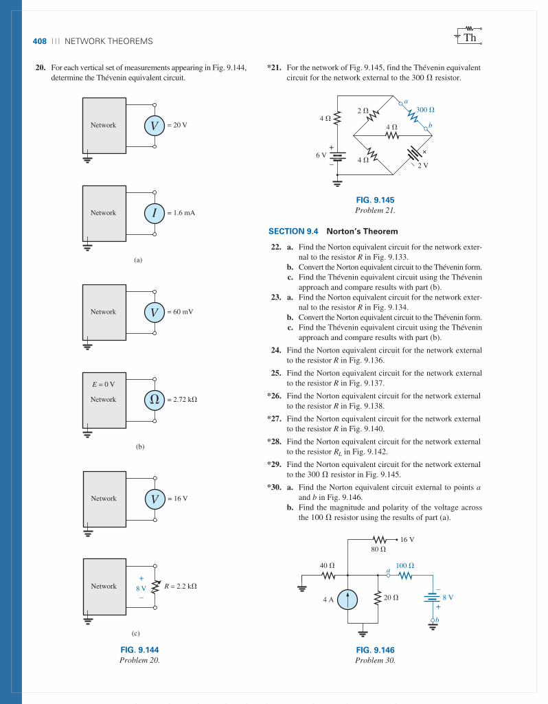
408 Network theorems Th
6 V
2
4
4
a
2 V
300
b4
+
–
+
–
FIG. 9.145Problem 21.
20. For each vertical set of measurements appearing in Fig. 9.144, determine the Thévenin equivalent circuit.
VNetwork = 20 V VNetwork = 60 mV VNetwork = 16 V
INetwork = 1.6 mA Network = 2.72 k Network R = 2.2 k
(a) (b) (c)
8 V
E = 0 V+
–
VNetwork = 20 V VNetwork = 60 mV VNetwork = 16 V
INetwork = 1.6 mA Network = 2.72 k Network R = 2.2 k
(a) (b) (c)
8 V
E = 0 V+
–
VNetwork = 20 V VNetwork = 60 mV VNetwork = 16 V
INetwork = 1.6 mA Network = 2.72 k Network R = 2.2 k
(a) (b) (c)
8 V
E = 0 V+
–
FIG. 9.144Problem 20.
*21. For the network of Fig. 9.145, find the Thévenin equivalent circuit for the network external to the 300 Ω resistor.
SECTION 9.4 Norton’s Theorem
22. a. Find the Norton equivalent circuit for the network exter-nal to the resistor R in Fig. 9.133.
b. Convert the Norton equivalent circuit to the Thévenin form. c. Find the Thévenin equivalent circuit using the Thévenin
approach and compare results with part (b). 23. a. Find the Norton equivalent circuit for the network exter-
nal to the resistor R in Fig. 9.134. b. Convert the Norton equivalent circuit to the Thévenin form. c. Find the Thévenin equivalent circuit using the Thévenin
approach and compare results with part (b).
24. Find the Norton equivalent circuit for the network external to the resistor R in Fig. 9.136.
25. Find the Norton equivalent circuit for the network external to the resistor R in Fig. 9.137.
*26. Find the Norton equivalent circuit for the network external to the resistor R in Fig. 9.138.
*27. Find the Norton equivalent circuit for the network external to the resistor R in Fig. 9.140.
*28. Find the Norton equivalent circuit for the network external to the resistor RL in Fig. 9.142.
*29. Find the Norton equivalent circuit for the network external to the 300 Ω resistor in Fig. 9.145.
*30. a. Find the Norton equivalent circuit external to points a and b in Fig. 9.146.
b. Find the magnitude and polarity of the voltage across the 100 Ω resistor using the results of part (a).
80
20
100
4 A
16 V
40
8 V
+
–
a
b
FIG. 9.146Problem 30.
GRIDLINE SET IN 1ST-PP TO INDICATE SAFE AREA; TO BE REMOVED AFTER 1ST-PP
M09_BOYL3605_13_SE_C09.indd Page 408 24/11/14 2:01 PM f403 /204/PH01893/9780133923605_BOYLESTAD/BOYLESTAD_INTRO_CIRCUIT_ANALYSIS13_SE_978013 ...

problems 409Th
*38. For the network in Fig. 9.150, determine the level of R that will ensure maximum power to the 100 Ω resistor. Find the maximum power to RL.
SECTION 9.5 Maximum Power Transfer Theorem
31. a. Find the value of R for maximum power transfer to R for the network of Fig. 9.133.
b. Determine the maximum power of R.
32. a. Find the value of R for maximum power transfer to R for the network of Fig. 9.136.
b. Determine the maximum power of R.
33. a. Find the value of R for maximum power transfer to R for the network of Fig. 9.138.
b. Determine the maximum power to R.
*34. a. Find the value of RL in Fig. 9.142 for maximum power transfer to RL.
b. Find the maximum power to RL.
35. a. For the network of Fig. 9.147, determine the value of R for maximum power to R.
b. Determine the maximum power to R. c. Plot a curve of power to R versus R for R ranging from
1/4 to 2 times the value determined in part (a) using an increment of 1/4 the value of R. Does the curve verify the fact that the chosen value of R in part (a) will ensure maximum power transfer?
20 V
5 A RR2
R1
E
I+
–
2.4
24
FIG. 9.147Problem 35.
*36. Find the resistance R1 in Fig. 9.148 such that the resistor R4 will receive maximum power. Think!
100 V 50 R4
R1
50 R2
50
R3
+
–
FIG. 9.148Problem 36.
*37. a. For the network in Fig. 9.149, determine the value of R2 for maximum power to R4.
b. Is there a general statement that can be made about situ-ations such as those presented here and in Problem 36?
120 V R4R2
24
R3
24
R1
E+
–
FIG. 9.149Problem 37.
12 V
RL
500 Pot.
R
100
+
–
FIG. 9.150Problem 38.
SECTION 9.6 Millman’s Theorem
39. Using Millman’s theorem, find the current through and volt-age across the resistor RL in Fig. 9.151.
40 V
6 R2
E1
RL 3
42 VE2
10 R1
+
–
+
–
FIG. 9.151Problem 39.
40. Repeat Problem 38 for the network in Fig. 9.152.
5 V 8.2 kR2E1
RL 5.6 k
20 VE2
+
–2.2 kR1
+
–
FIG. 9.152Problem 40.
GRIDLINE SET IN 1ST-PP TO INDICATE SAFE AREA; TO BE REMOVED AFTER 1ST-PP
M09_BOYL3605_13_SE_C09.indd Page 409 24/11/14 2:01 PM f403 /204/PH01893/9780133923605_BOYLESTAD/BOYLESTAD_INTRO_CIRCUIT_ANALYSIS13_SE_978013 ...

410 Network theorems Th
45. Using the substitution theorem, draw three equivalent branches for the branch a-b of the network in Fig. 9.157.
41. Using Millman’s theorem, find the current through and voltage across the resistor RL in Fig. 9.153.
+
–
400 V 50 R2E1
20 VE2
+
–80 R1
RL 200 10 VE3
+
–
R3
50
FIG. 9.153Problem 41.
42. Using the dual of Millman’s theorem, find the current through and voltage across the resistor RL in Fig. 9.154.
R1
4.7 RL 2.7
I1 = 4 A
R2
3.3
I2 = 1.6 A
FIG. 9.154Problem 42.
43. Using the dual of Millman’s theorem, find the current through and voltage across the resistor RL in Fig. 9.155.
R2
4.7
8 mA
I2
I1
10 mA
R1 2 k I3
4 mA
R3 8.2 k
6.8 k
RL
FIG. 9.155Problem 43.
SECTION 9.7 Substitution Theorem
44. Using the substitution theorem, draw three equivalent branches for the branch a-b of the network in Fig. 9.156.
7 k15 k60 VE
8 k2.5 k a
b
+
–
FIG. 9.156Problem 44.
2 k 1.5 k
R2
0.51 k
4 mA
I
10 V
Eba
R1
+ –
FIG. 9.157Problem 45.
*46. Using the substitution theorem, draw three equivalent branches for the branch a-b of the network of Fig. 9.158.
R2 12 20 VE1
8 4 a
b
40 VE2
R3R1
+
– +
–
FIG. 9.158Problem 46.
SECTION 9.8 Reciprocity Theorem
47. a. For the network in Fig. 9.159(a), determine the current I. b. Repeat part (a) for the network in Fig. 9.159(b). c. Is the reciprocity theorem satisfied?
24 VE
4 k8 k
24 k20 k
24 k
I
(a)
24 V
E
4 k8 k
24 k
24 k
I
(b)
+
–
+
–
20 k
24 VE
4 k8 k
24 k20 k
24 k
I
(a)
24 V
E
4 k8 k
24 k
24 k
I
(b)
+
–
+
–
20 k
FIG. 9.159Problem 47.
GRIDLINE SET IN 1ST-PP TO INDICATE SAFE AREA; TO BE REMOVED AFTER 1ST-PP
M09_BOYL3605_13_SE_C09.indd Page 410 24/11/14 2:01 PM f403 /204/PH01893/9780133923605_BOYLESTAD/BOYLESTAD_INTRO_CIRCUIT_ANALYSIS13_SE_978013 ...

Glossary 411Th
GLOSSARY
Maximum power transfer theorem A theorem used to deter-mine the load resistance necessary to ensure maximum power transfer to the load.
Millman’s theorem A method using source conversions that will permit the determination of unknown variables in a multiloop network.
Norton’s theorem A theorem that permits the reduction of any two-terminal linear dc network to one having a single current source and parallel resistor.
Reciprocity theorem A theorem that states that for single-source networks, the current in any branch of a network due to a single voltage source in the network will equal the current through the branch in which the source was originally located if the source is placed in the branch in which the current was originally measured.
Substitution theorem A theorem that states that if the voltage across and current through any branch of a dc bilateral net-work are known, the branch can be replaced by any combina-tion of elements that will maintain the same voltage across and current through the chosen branch.
Superposition theorem A network theorem that permits consid-ering the effects of each source independently. The resulting current and/or voltage is the algebraic sum of the currents and/or voltages developed by each source independently.
Thévenin’s theorem A theorem that permits the reduction of any two-terminal, linear dc network to one having a single voltage source and series resistor.
48. a. For the network of Fig. 9.160(a), determine the current I. b. Repeat part (a) for the network in Fig. 9.160(b). c. Is the reciprocity theorem satisfied?
49. a. Determine the voltage V for the network in Fig. 9.161(a). b. Repeat part (a) for the network in Fig. 9.161(b). c. Is the dual of the reciprocity theorem satisfied?
+–
+
–
4 k 4 k
4 k 8 k
E
10 V
I
(a)
4 k 4 k
4 k 8 k
E 10 VI
(b)
+–
+
–
4 k 4 k
4 k 8 k
E
10 V
I
(a)
4 k 4 k
4 k 8 k
E 10 VI
(b)
FIG. 9.160Problem 48.
R1 3
R2
2
R3 4 I
6 A
+ V –
(a)
R1 3
R2
2
R3 4
I = 6 A
V
(b)
+
–
R1 3
R2
2
R3 4 I
6 A
+ V –
(a)
R1 3
R2
2
R3 4
I = 6 A
V
(b)
+
–
FIG. 9.161Problem 49.
SECTION 9.9 Computer Analysis
50. Using PSpice or Multisim and the superposition theorem, determine the voltage V2 and its components for the net-work in Fig. 9.130.
51. Using PSpice or Multisim, determine the Thévenin equiva-lent circuit for the network in Fig. 9.138.
*52. a. Using PSpice, plot the power delivered to the resistor R in Fig. 9.135 for R having values from 1 Ω to 10 Ω.
b. From the plot, determine the value of R resulting in the maximum power to R and the maximum power to R.
c. Compare the results of part (a) to the numerical solution. d. Plot VR and IR versus R, and find the value of each under
maximum power conditions.
*53. Change the 300 Ω resistor in Fig. 9.145 to a variable resis-tor, and using Pspice, plot the power delivered to the resis-tor versus values of the resistor. Determine the range of resistance by trial and error rather than first performing a longhand calculation. Determine the Norton equivalent cir-cuit from the results. The Norton current can be determined from the maximum power level.
GRIDLINE SET IN 1ST-PP TO INDICATE SAFE AREA; TO BE REMOVED AFTER 1ST-PP
M09_BOYL3605_13_SE_C09.indd Page 411 24/11/14 2:01 PM f403 /204/PH01893/9780133923605_BOYLESTAD/BOYLESTAD_INTRO_CIRCUIT_ANALYSIS13_SE_978013 ...

M09_BOYL3605_13_SE_C09.indd Page 412 24/11/14 2:01 PM f403 /204/PH01893/9780133923605_BOYLESTAD/BOYLESTAD_INTRO_CIRCUIT_ANALYSIS13_SE_978013 ...
Related Documents