Network Inference - julien.cremeriefamily.infojulien.cremeriefamily.info/doc/teachings/ips2/td_ips2_correction.pdf · Network Inference [email protected],[email protected]

Network Inference

[email protected], [email protected]

Summer School 2016 - From gene expression to genomic network

This practical aims to provide a quick overview of sparse Gaussian GraphicalModels (GGM) and their use in the context of network reconstruction for geneinteraction networks.

To this end, we rely on the R-package huge, which implements some of the mostpopular sparse GGM methods and provides a set of basic tools for their handlingand their analysis.

The first part focuses on an empirical analysis of the statistical models used fornetwork reconstruction. The objective is to quickly study the range of applicabilityof these methods. It should also give you some insights about their limitations,especially toward the interpretability of the inferred network in terms of biology.

The second part applies these methods to two data sets: the first one consists in atranscriptomic data associated to a small regulatory network (tens of genes) knownby the biologists. The second one is a large cohort of breast cancer transcriptomicdata set associated to 44,000 transcripts. The objective is to unravel the moststriking interactions between differentially expressed genes.

Note : you can form small and balanced groups of students to work. Some functionrequired during the session are available in file external_functions.R (ask theteachers).

1 First part: empirical study of sparse GGM

Load the huge package. Have a quick glance at the help.

1.1 Synthetic data generation, Network representation

The function huge.generator allows to generate a random network and some(expression) data associated with this network.

1

mailto:[email protected]

mailto:[email protected]

— Use this function to generate a simple random network with the size ofyour choice. Have a look at the structure of the R object produced by thefunction.

n <- 50; d <- 100

random.net <- huge.generator(n, d, graph="random")

## Generating data from the multivariate normal distribution with the random graph structure....done.

str(random.net, max.level = 1)

## List of 7

## $ data : num [1:50, 1:100] -0.519 0.155 -0.78 0.405 1.277 ...

## ..- attr(*, "dimnames")=List of 2

## $ sigma : num [1:100, 1:100] 1 -0.00245 0.0076 -0.0102 -0.00138 ...

## $ sigmahat : num [1:100, 1:100] 1 0.1211 0.1369 -0.1133 0.0594 ...

## $ omega : num [1:100, 1:100] 1.17 -2.92e-18 5.05e-18 1.84e-18 -9.31e-19 ...

## $ theta :Formal class 'dsCMatrix' [package "Matrix"] with 7 slots

## $ sparsity : num 0.0315

## $ graph.type: chr "random"

## - attr(*, "class")= chr "sim"

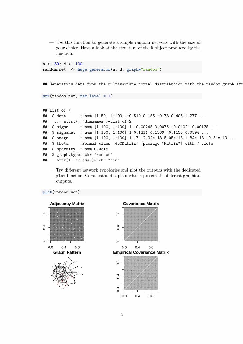
— Try different network typologies and plot the outputs with the dedicatedplot function. Comment and explain what represent the different graphicaloutputs.

plot(random.net)

0.0 0.4 0.8

0.0

0.4

0.8

Adjacency Matrix

0.0 0.4 0.8

0.0

0.4

0.8

Covariance Matrix

Graph Pattern

0.0 0.4 0.8

0.0

0.4

0.8

Empirical Covariance Matrix

2

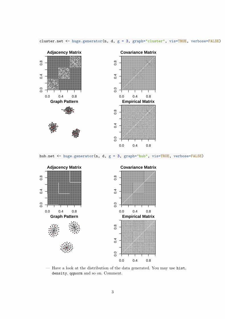
cluster.net <- huge.generator(n, d, g = 3, graph="cluster", vis=TRUE, verbose=FALSE)

0.0 0.4 0.8

0.0

0.4

0.8

Adjacency Matrix

0.0 0.4 0.8

0.0

0.4

0.8

Covariance Matrix

Graph Pattern

0.0 0.4 0.8

0.0

0.4

0.8

Empirical Matrix

hub.net <- huge.generator(n, d, g = 3, graph="hub", vis=TRUE, verbose=FALSE)

0.0 0.4 0.8

0.0

0.4

0.8

Adjacency Matrix

0.0 0.4 0.8

0.0

0.4

0.8

Covariance Matrix

Graph Pattern

0.0 0.4 0.8

0.0

0.4

0.8

Empirical Matrix

— Have a look at the distribution of the data generated. You may use hist,density, qqnorm and so on. Comment.

3

expr <- random.net$data

par(mfrow=c(1,2))

hist(expr, probability = TRUE)

lines(density(expr), col="red", lwd=2)

qqnorm(expr); qqline(expr)

Histogram of expr

expr

Den

sity

−2 0 2 4

0.0

0.1

0.2

0.3

−4 −2 0 2 4

−2

02

4

Normal Q−Q Plot

Theoretical Quantiles

Sam

ple

Qua

ntile

s

Real life is (hopefully) not that easy.

— How can you change the level of difficulty in the problem of networkreconstruction?

1.2 Correlation vs. Partial correlation

This section aims to illustrate the difference of relationship modeled by correlationand partial correlation.

— generate a graph with d = 10 nodes, a single hub, and expression data withn = 200 samples. We are going to study the statistical relationship betweenthe hub (first node in your graph) and 2 of its neighbors. We call hub theindex of the hub and neighbor1, neighbor2 the label (index) of these threenodes.

set.seed(1)

exp <- huge.generator(n=200, d=10, grap="hub",verbose=FALSE)

hub <- 1

neighbors <- which(exp$theta[, hub] != 0)

neighbor1 <- neighbors[1]; neighbor2 <- neighbors[2]

— Adjust three simple linear regressions between the data associated withthese three nodes, that is, between hub and neighbor1, hub and neighbor2,and neighbor1 and neighbor2. Use the function lm + summary to test thesignificance of each model. Comment.

4

## all significant correlations

summary(lm(exp$data[, hub]~exp$data[, neighbor1]))

##

## Call:

## lm(formula = exp$data[, hub] ~ exp$data[, neighbor1])

##

## Residuals:

## Min 1Q Median 3Q Max

## -2.62573 -0.62038 0.01327 0.52993 2.50639

##

## Coefficients:

## Estimate Std. Error t value Pr(>|t|)

## (Intercept) 0.04618 0.06820 0.677 0.499

## exp$data[, neighbor1] -0.35470 0.06456 -5.494 1.2e-07 ***

## ---

## Signif. codes: 0 '***' 0.001 '**' 0.01 '*' 0.05 '.' 0.1 ' ' 1

##

## Residual standard error: 0.9645 on 198 degrees of freedom

## Multiple R-squared: 0.1323, Adjusted R-squared: 0.1279

## F-statistic: 30.19 on 1 and 198 DF, p-value: 1.196e-07

summary(lm(exp$data[, hub]~exp$data[, neighbor2]))

##

## Call:

## lm(formula = exp$data[, hub] ~ exp$data[, neighbor2])

##

## Residuals:


## -2.26976 -0.61419 -0.02027 0.59983 2.22808

##

## Coefficients:


## (Intercept) 0.04358 0.06257 0.697 0.487

## exp$data[, neighbor2] -0.54373 0.06358 -8.551 3.29e-15 ***

## ---

## Signif. codes: 0 '***' 0.001 '**' 0.01 '*' 0.05 '.' 0.1 ' ' 1

##



## F-statistic: 73.13 on 1 and 198 DF, p-value: 3.294e-15

summary(lm(exp$data[, neighbor1]~exp$data[, neighbor2]))

##

5

## Call:

## lm(formula = exp$data[, neighbor1] ~ exp$data[, neighbor2])

##

## Residuals:


## -2.93658 -0.68953 -0.02216 0.64551 2.96591

##

## Coefficients:


## (Intercept) -0.00501 0.07327 -0.068 0.94556

## exp$data[, neighbor2] 0.23474 0.07445 3.153 0.00187 **

## ---

## Signif. codes: 0 '***' 0.001 '**' 0.01 '*' 0.05 '.' 0.1 ' ' 1

##



## F-statistic: 9.941 on 1 and 198 DF, p-value: 0.001868

This experiment shows that the expression of the neighbors are potentially cor-related, although there is no direct link between them. As will be seen, partialcorrelation avoid such a spurious interaction.

— Partial correlation corresponds to correlation that remains between pairsof variables once remove the effect of the others variables. To test directrelationships between two neighbors, with thus have to remove the effect ofall others variables. To do so, adjust two multiple linear model to predictthe expression of the two neighbors by all the others genes but them.

lm1 <- lm(exp$data[,neighbor1]~exp$data[,-c(neighbor1,neighbor2)])

lm2 <- lm(exp$data[,neighbor2]~exp$data[,-c(neighbor1,neighbor2)])

— Get back the residuals associated with each model. This corresponds towhat is not predicted in the expression of each neighbor by all the genesbut neighbor1 and neighbor2.

neighbor1.res <- residuals(lm1)

neighbor2.res <- residuals(lm2)

— Adjust simple linear regression between the residuals and test the significanceof this model. Comment

## no significant partial correlation

summary(lm(neighbor1.res~neighbor2.res))

##

## Call:

## lm(formula = neighbor1.res ~ neighbor2.res)

##

6

## Residuals:


## -2.9372 -0.6478 0.0019 0.5966 2.7740

##

## Coefficients:


## (Intercept) -2.722e-17 6.917e-02 0.000 1.000

## neighbor2.res 2.548e-02 8.367e-02 0.304 0.761

##


## Multiple R-squared: 0.000468, Adjusted R-squared: -0.00458

## F-statistic: 0.0927 on 1 and 198 DF, p-value: 0.7611

— Use the geom_smooth function in the package ggplot2 to adjust and re-present the four simple linear regression models fitted so far and summaryyour experiment.

multiplot(qplot(exp$data[, hub], exp$data[, neighbor1], geom="point") + geom_smooth(method="lm"),

qplot(exp$data[, hub], exp$data[, neighbor2], geom="point") + geom_smooth(method="lm"),

qplot(exp$data[, neighbor1], exp$data[, neighbor2], geom="point") + geom_smooth(method="lm"),

qplot(neighbor1.res,neighbor2.res, geom="point") + geom_smooth(method="lm"), cols = 2)

−2

0

2

−2 0 2exp$data[, hub]

exp$

data

[, ne

ighb

or1]

−2

−1

0

1

2

−2 0 2exp$data[, hub]

exp$

data

[, ne

ighb

or2]

−2

−1

0

1

2

−2 0 2exp$data[, neighbor1]

exp$

data

[, ne

ighb

or2]

−2

−1

0

1

2

−3 −2 −1 0 1 2 3neighbor1.res

neig

hbor

2.re

s

1.2.1 Network inference accuracy

Now, to the network reconstruction at last ! The function huge automatically selectthe most significant partial correlation between variables, by adjusting a sparseGGM to the data. The final number of interactions (i.e., the number of edge in thereconstructed network) is controlled by a tuning parameter, the choice of whichcan be obtained by cross-validation.

7

We want to study the effect of the sample size on the performance of two methods:the sparse GGM approach (hereafter glasso) and the simple correlation approach,which just consists in thresholding the matrix of empirical correlations.

— The following function one.simu performs a simulation by computing thearea under ROC curve for the glasso and the correlation based approachfrom a data set generated with the huge.generator function. The numberof genes is 25, and the sample size varies from 5 to 500. Read it, try tounderstand it. . .

require(reshape2)

one.simu <- function(i) {

cat("n =")

d <- 25; seq.n <- c(5,15,30,50,100,250,500)

out <- data.frame(t(sapply(seq.n, function(n) {

cat("",n)

exp <- huge.generator(n, d, verbose=FALSE)

glasso <- huge(exp$data, method="glasso", verbose=FALSE)

corthr <- huge(exp$data, method="ct", verbose=FALSE)

res.corthr <- perf.auc(perf.roc(corthr$path, exp$theta))

res.glasso <- perf.auc(perf.roc(glasso$path, exp$theta))

return(setNames(c(res.glasso,res.corthr,n,i),

c("glasso","correlation","sample size", "simu")))

})))

return(melt(out, measure.vars = 1:2, value.name = "score"))

}

— Use this function to perform one single simulation and represent the evolutionof the AUC for each method as a function of the sample size.

out <- one.simu(1)

## n = 5 15 30 50 100 250 500

ggplot(out, aes(x=sample.size, y=score,group=variable,colour=variable)) +

geom_point(alpha=.5) + coord_trans(x="log10")

8

0.6

0.7

0.8

0.9

100 200 300 400500sample.size

scor

e

variable

glasso

correlation

— Perform a bunch (say 30) simulations and represent the boxplots of theAUC for each method and as a function of the sample size. You may usethe parallel package with its function mclapply. (or doMC and foreach ifyou work with Windows). This might take some time, so check your codeand be patient!

library(parallel)

res <- do.call(rbind, mclapply(1:50, one.simu))

ggplot(res, aes(x=factor(sample.size), y=score)) +

geom_point(alpha=.5, aes(group=variable,colour=variable)) +

geom_boxplot(aes(colour=variable))

0.6

0.8

1.0

5 15 30 50 100 250 500factor(sample.size)

scor

e

variable

glasso

correlation

9

2 Second part: transcriptomic data analysis

2.1 Inferring a network from transcriptomic data, normalization?

Now we will have look at the gene expression levels of 16 genes part of the corenetwork identified by Francoise Moneger and her colleagues. In total we have 20measurements : 2 times 10 biological replicates of flower bud.

First, load the data and the network identified by Francoise Moneger and colleagues.(the network is store as 16 x 16 contingency matrix).

load( file="data_school/Expr.RData")

load(file="data_school/Netw_FM.RData")

Then load a few usufull functions

### Inference

source("external_functions.R")

require(huge)

### a simple function thresholding a matrix for nlambda values

### between the min and max value (outside of the diagonal)

cor.thres <- function(C.mat){

diag(C.mat) <- 0

C.mat <- abs(C.mat)

lvls <- c(0, unique(C.mat), max(C.mat)+1)

res <- lapply( lvls,

FUN=function(thres) ((C.mat >= thres)+0))

}

2.1.1 Inferring the network with sparse GGM or correlation network

Infer the network using correlation or glasso and draw the ROC of the twoapproaches.

## pearson correlation approach

res.cor <- cor.thres(cor(X))

## glasso and grid of lambda

min.lbd <- 100

lambdas <- rev(1/min.lbd * 10^seq(0, log10(min.lbd), length.out=1000))

res.glasso <- huge((X), method="glasso", lambda=lambdas, verbose=F)

## computing the roc curve

roc.cor <- perf.roc(res.cor, trueNetMat)

roc.glasso <- perf.roc(res.glasso$path, trueNetMat)

10

roc.cor$method <- "cor"

roc.glasso$method <- "glasso"

## plotting

require(ggplot2)

data <- rbind(roc.cor, roc.glasso)

p <- ggplot(data, aes(x=fallout, y=recall, group=method)) +

geom_line(aes(colour = method))

p

0.00

0.25

0.50

0.75

1.00

0.00 0.25 0.50 0.75 1.00fallout

reca

ll

method

cor

glasso

2.1.2 Normalisation and network inference

The huge package provides various way to pre-process the data (andtry to make them more “normal”). Try to use the “skeptic” approach(huge.npn(X,npn.func="skeptic")) and draw its ROC curve. What doyou conclude ?

Q=(huge.npn(X, npn.func="skeptic"))

## Conducting nonparanormal (npn) transformation via skeptic....done.

min.lbd <- 100


res.glasso.skeptic <- huge(Q,

method="glasso", lambda=lambdas, verbose=F)

roc.glasso.skeptic <- perf.roc(res.glasso.skeptic$path, trueNetMat)

roc.glasso.skeptic$method <- "glasso.skeptic"

11

## plotting

data <- rbind(roc.cor, roc.glasso, roc.glasso.skeptic)



p

0.00

0.25

0.50

0.75

1.00

0.00 0.25 0.50 0.75 1.00fallout

reca

ll

method

cor

glasso

glasso.skeptic

Figure 1 – Glasso, Correlation and Glasso+skeptic

2.1.3 Inversion correlation ?

Given the number of samples we could also try to inverse the correlation matrixdirectly. Try this other approach and draw its ROC curve and conclude.

res.inv <- cor.thres(solve(cor(X)))

roc.inv <- perf.roc(res.inv, trueNetMat)

roc.inv$method <- "inv"

## plotting

data <- rbind(roc.cor, roc.inv, roc.glasso.skeptic)



p

2.2 Differential analysis and gene networks

Now we will look at some data from Guedj et al. (2011). In this data there are twogroups ER positive breast tumors and ER negative breast tumors. A number ofgenes are differentially expressed between these two groups.

12

0.00

0.25

0.50

0.75

1.00

0.00 0.25 0.50 0.75 1.00fallout

reca

ll

method

cor

glasso.skeptic

inv

Figure 2 – Correlation and inverse correlation

We will first load the data

load ("data_school/breast_cancer_guedj11.RData") # raw data

load ("data_school/gen_name.RData") # each row of the raw data matrix is a gene.

gene.name <- unlist(gene.name)

data.raw <- expr

2.2.1 Differential analysis

Run limma or a t.test analysis to compare the two groups. Assess the number ofsignificant genes (with an adjusted p-value below 0.05).

## limma analysis

require(limma)

## Loading required package: limma

design <- cbind(Moy=1, Erp=(class.ER == "ERp")+0)

fit <- lmFit(data.raw, design=design)

fit <- eBayes(fit)

res <- topTable(fit, coef="Erp", number=10^5, genelist=fit$genes, adjust.method="BH",

sort.by="none", resort.by=NULL, p.value=1, lfc=0, confint=FALSE)

## checking the distribution of p-values

hist(res$P.Value, breaks=30, col="grey")

13

Histogram of res$P.Value

res$P.Value

Fre

quen

cy

0.0 0.2 0.4 0.6 0.8 1.0

050

0015

000

2500

0

## a lot of differentially expressed genes

sum(res$adj.P.Val <= 0.05)

## [1] 26661

sum(res$adj.P.Val <= 10^-10)

## [1] 1840

2.2.2 Network inference

Infer a network for each group using the first p=100 most differentially expressedgenes. Check the shape of the ebic to assess the quality of the inference and thegrid of lambdas.

min.lbd <- 100


selected_gene <- order(res$P.Value)[1:100] ## top 100 genes from diff analysis

require(huge)

data.ERm <- t(data.raw[selected_gene, which(class.ER=="ERm")])

data.ERp <- t(data.raw[selected_gene, which(class.ER=="ERp")])

gl.ERm <- huge(data.ERm, method="glasso", lambda=lambdas, verbose=F)

gl.ERp <- huge(data.ERp, method="glasso", lambda=lambdas, verbose=F)

sel.ERm <- huge.select(gl.ERm)

## Conducting extended Bayesian information criterion (ebic) selection....done

14

sel.ERp <- huge.select(gl.ERp)

## Conducting extended Bayesian information criterion (ebic) selection....done

### check bic curve to know how many genes to take

par(mfrow=c(1,2))

plot(log10(sel.ERm$lambda), sel.ERm$ebic.score)

plot(log10(sel.ERp$lambda),sel.ERp$ebic.score)

−2.0 −1.0 0.0

1500

025

000

3500

0

log10(sel.ERm$lambda)

sel.E

Rm

$ebi

c.sc

ore

−2.0 −1.0 0.0

3500

040

000

4500

050

000

log10(sel.ERp$lambda)

sel.E

Rp$

ebic

.sco

re

2.2.3 ESR1 edges in ER positive tumors

Identify ESR1 edges that are only present in ER positive tumors.

## ESR1 is the first gene

toLookAt <- which(sel.ERp$refit[1, ] ==1 & sel.ERm$refit[1,] ==0)

output.test <- data.frame(name=gene.name[selected_gene][toLookAt],

icov = sel.ERp$opt.icov[1, toLookAt],

logFC = res$logFC[selected_gene][toLookAt],

pvalue= res$P.Value[selected_gene][toLookAt]

)

for(i in 2:4) output.test[, i] <- signif(output.test[, i], 3)

output.test

## name icov logFC pvalue

## 215867_x_at CA12 -0.00161 2.050 5.42e-52

## 204667_at FOXA1 -0.15700 1.650 1.63e-39

## 200670_at XBP1 -0.02750 0.930 1.44e-36

## 226506_at THSD4 -0.08220 1.110 4.33e-33

## 205355_at ACADSB -0.00692 1.220 5.74e-33

## 204798_at MYB -0.17600 1.340 4.40e-31

15

## 220559_at EN1 0.06660 -1.280 9.75e-30

## 227262_at HAPLN3 0.11200 -0.499 8.36e-29

## 226197_at AR -0.04950 1.330 2.58e-28

## 200810_s_at CIRBP 0.04760 0.604 4.00e-28

## Not.Known -0.10100 0.982 6.84e-28

## 219497_s_at BCL11A 0.05110 -1.310 1.34e-27

## 225911_at NPNT -0.00380 1.490 4.85e-27

2.2.4 Stability of those edges

Assess whether those edges are stable using resampling. Search “FOXA1” in googlescholar or entrez.

data.ERm <- t(data.raw[selected_gene, which(class.ER=="ERm")])

data.ERp <- t(data.raw[selected_gene, which(class.ER=="ERp")])

one.resample <- function(i_, prop=0.9){

## print(i_)

n.X <- nrow(data.ERm)

n.Y <- nrow(data.ERp)

X <- data.ERm[sample.int(n.X, size=trunc(0.9*n.X)), ]

Y <- data.ERp[sample.int(n.Y, size=trunc(0.9*n.Y)), ]

gl.ERm <- huge(X, method="glasso", nlambda=100, verbose=F)

gl.ERp <- huge(Y, method="glasso", nlambda=100, verbose=F)

sel.ERm <- huge.select(gl.ERm, verbose=F)

sel.ERp <- huge.select(gl.ERp, verbose=F)

return(sel.ERp$refit[1, ] ==1 & sel.ERm$refit[1,] ==0)

}

require(parallel)

## Loading required package: parallel

stability_res <- mclapply(1:100, FUN=one.resample, mc.cores=1)

proba.out <- rowMeans(do.call("cbind", stability_res))

toLookAt <- which(proba.out > 0.95)

output.test <- data.frame(name=gene.name[selected_gene][toLookAt],

icov = sel.ERp$opt.icov[1, toLookAt],

logFC = res$logFC[selected_gene][toLookAt],

pvalue= res$P.Value[selected_gene][toLookAt],

proba=proba.out[toLookAt]

)

for(i in 2:4) output.test[, i] <- signif(output.test[, i], 3)

output.test

16

## name icov logFC pvalue proba

## 204667_at FOXA1 -0.1570 1.650 1.63e-39 1.00

## 220559_at EN1 0.0666 -1.280 9.75e-30 1.00

## 227262_at HAPLN3 0.1120 -0.499 8.36e-29 1.00

## 226197_at AR -0.0495 1.330 2.58e-28 0.99

## 200810_s_at CIRBP 0.0476 0.604 4.00e-28 0.98

## Not.Known -0.1010 0.982 6.84e-28 1.00

## 219497_s_at BCL11A 0.0511 -1.310 1.34e-27 1.00

2.2.5 Correlation

Compute the correlation between ESR1 and the top 100 genes in ER positive andER negative tumors. Look at FOXA1.

## looking at the correlation

cor_data <- data.frame(name=gene.name[selected_gene],

cor.inneg = signif(cor(data.ERm)[1, ], 3),

cor.inpos = signif(cor(data.ERp)[1, ])

)

hist(cor_data$cor.inneg - cor_data$cor.inpos, col="grey", main="FOXA1?")

abline(v=cor_data$cor.inneg[13] - cor_data$cor.inpos[13], col="blue")

FOXA1?

cor_data$cor.inneg − cor_data$cor.inpos

Fre

quen

cy

−0.4 −0.2 0.0 0.2 0.4 0.6

010

2030

17

Network Inference - julien.cremeriefamily.infojulien.cremeriefamily.info/doc/teachings/ips2/td_ips2_correction.pdf · Network Inference [email protected],[email protected]

Documents