Network Connectivity with a Family of Group Mobility Models

IEEE TRANSACTIONS ON MOBILE COMPUTING 1

Network Connectivity with a Family of GroupMobility Models

Richard J. La and Eunyoung Seo

Abstract—We investigate the communication range of thenodes necessary for network connectivity, which we call bi-directional connectivity, in a simple setting. Unlike in most ofexisting studies, however, the locations or mobilities of the nodesmay be correlated through group mobility: Nodes are brokeninto groups, with each group comprising the same number ofnodes, and lie on a unit circle. The locations of the nodes inthe same group are not mutually independent, but are insteadconditionally independent given the location of the group.

We examine the distribution of the smallest communicationrange needed for bi-directional connectivity, called the criticaltransmission range (CTR), when both the number of groups andthe number of nodes in a group are large. We first demonstratethat the CTR exhibits a parametric sensitivity with respect tothe space each group occupies on the unit circle. Then, we offeran explanation for the observed sensitivity by identifying whatis known as a very strong threshold and asymptotic bounds forCTR.

Index Terms—Mobile communication systems; Wireless com-munication networks; Network connectivity..

I. INTRODUCTION

Mobile ad-hoc networks (MANETs) or multi-hop wirelessnetworks (MHWNs) have attracted much interest from thenetworking community, due to their potential for numerousapplications. In a traditional wired network, traffic generatedby so-called end nodes is routed through the network bydedicated routers. However, in a MANET wireless nodesform and maintain the network and share the responsibility ofrouting packets from sources to destinations. Moreover, when(some of) nodes are mobile, the one-hop connectivity, hencetopology, of the network varies with time. This requires thenetwork protocols to cope with potentially frequent changesin network topology.

When information to be transferred by a MHWN cannottolerate large delays, timely delivery of information demandsthat the network be able to find an end-to-end route between asource and a destination. In order for such an end-to-end routeto exist when one is needed, the network should be connected(with a high probability). For this reason the issue of networkconnectivity enjoyed much attention in recent years.

In some cases, nodes may have access to a replenishedenergy source and interference between simultaneous trans-missions may not be a concern (e.g., light traffic scenarios).In such cases, network connectivity can be dealt with byemploying the largest transmit power at the nodes. In othercases, however, especially when some of the mobile nodes

This work was supported by the National Science Foundation underGrant CCF 08-30702, the U.S. Army Research Laboratory (ARL), and theLaboratory for Telecommunications Sciences (LTS).

Authors are with the Department of Electrical and Computer Engineeringand the Institute for Systems Research at the University of Maryland, CollegePark. E-mail: hyongla, [email protected]

operate on batteries, this may not be an acceptable solution; itis likely to result in unnecessarily quick depletion of batterypower. In these scenarios, it is in the interest of the batterypowered nodes to use the minimum necessary transmit power,which will result in a smaller communication range betweennodes, so as to conserve energy.

Another, perhaps, less obvious reason why nodes may wantto employ smaller communication ranges through transmitpower control stems from the study of network transportthroughput: Gupta and Kumar showed in their seminal paper[10] that, in order for the nodes to maximize the networkthroughput, they should adopt the smallest communicationrange to maintain network connectivity. The basic intuition isthat employing the smallest communication range allows forthe maximum spatial reuse of the spectrum by minimizing theinterference caused to nearby nodes.

A natural question that arises under these arguments is:“What is the smallest communication range needed for net-work connectivity?” In order to study the connectivity prop-erties of MHWNs, researchers often represent the one-hopconnectivity of the network as a random graph and investigatethe connectivity of the graph. Study of connectivity propertyof random graphs dates back to late 1950’s, starting with thepioneering work by Erdos and Renyi [6], [7].

More recently, another line of research more related tothe connectivity of MHWNs examined various properties ofgeometric random graphs, including their connectivity (e.g.,[1], [9], [12], [13], [18], [22], [24], [26]). We refer interestedreaders to a monograph by Penrose [21]. In a geometricrandom graph, one-hop connectivity between a pair of nodesis determined by the distance between them. In other words,there exists an edge between two nodes i and j if and only iftheir distance is smaller than some threshold γ. This thresholdγ can be interpreted as a proxy to a common communicationor transmission range of the nodes, which depends on theemployed transmit power, in the context of MHWNs [23].

The one-hop connectivity model in geometric randomgraphs has been generalized in different ways, in order tocapture, for instance, environmental factors in one-hop con-nectivity between a pair of nodes given transmit power (e.g.,[17], [25]). In addition, Diaz et al. [5] studied the dynamiccase where nodes move according to a mobility model similarto the Random Direction models [3], [20]. They computed theexpected duration of a period during which a network remainsconnected or disconnected under the one-hop connectivitymodel of random geometric graphs.

Most of existing studies on connectivity of geometric ran-dom graph models, however, focus on the scenarios wherethe locations of the nodes are independent of each otherwith identical spatial distribution (e.g., [1], [9], [12], [22],

IEEE TRANSACTIONS ON MOBILE COMPUTING 2

[24], [26]). The dynamic case studied in [5] also assumesindependent and homogeneous node mobility. Unfortunately,when either of these assumptions is relaxed, little is knownabout the connectivity property of random graphs. In thispaper, we take another step towards better understandingconnectivity when nodes’ mobility is correlated.

A. Summary of setup

We consider simple scenarios where nodes are placed on aunit ring.1 Such one-dimensional cases may be of interest, forinstance, in vehicular ad-hoc networks on freeways [2]. Unlikein the independent cases, however, these nodes are broken intoa number of groups containing the same number of members.While the locations of two nodes in two different groups areindependent, those of two nodes in the same group are onlyconditionally independent given the location of the group.

All members of a group lie on an arc (on the unit ring)with a fixed length d, 0 ≤ d ≤ 1. Hence, the distance betweenany two members of a group2 is upper bounded by d. Here,the length d of the arc occupied by the members of a groupdetermines how strongly their locations are correlated; thesmaller d is, the stronger the correlation is.

One-hop connectivity between nodes is modeled usinga geometric random graph [21]: Two nodes have a (bi-directional) communication link between them if and only ifthe distance between them is not larger than some constantγ. As mentioned earlier, we can view this constant γ as aproxy to a common communication or transmission range ofthe nodes. Two nodes that are within γ are called neighbors.We briefly discuss in subsection IV-D how our findings basedon the geometric random graph model can be extended to amore general one-hop connectivity model called a quasi-unitdisk model [17].

In this paper, we adopt a slightly stronger notion ofconnectivity (than so-called 1-edge connectivity), which wecall bi-directional connectivity; a network is bi-directionallyconnected if it is possible to reach any node from anyother node by visiting a sequence of neighbors both in aclockwise direction and in a counter-clockwise direction. Weare interested in investigating how the smallest γ that resultsin a bi-directionally connected network, which we call acritical transmission range (CTR), behaves as the network sizebecomes large, i.e., both the number of groups and the numberof members in a group are large.

Unfortunately, finding the exact distribution of CTR for aspecific number of nodes in the network is difficult, if possibleat all. Instead, we study an asymptotic case as both the numberof groups (G) and the number of members in each group (M )increase. As the number of nodes grows, the distribution ofCTR becomes concentrated over a short interval that is easierto identify or approximate. Such findings in turn can be usedto provide network engineers with a guideline for choosing

1We select a unit ring instead of a unit interval to avoid the boundary effects.However, numerical results reported in Section V suggest that the (distributionof the) smallest communication range required for network connectivity issimilar for both the unit ring and the unit interval.

2The distance between two nodes is given by the length of the shorter arc(along the unit circle) that connects the two nodes.

suitable communication ranges for large networks. In addition,it may offer some idea as to how much transmit power may berequired at some nodes, hence, necessary energy consumption.

B. Summary of main contributions

We summarize the main findings as follows:• First, we illustrate the sensitivity of CTR to the parameterd (length of the arc occupied by a group) over some inter-val. In particular, we provide a numerical example wherethe median CTR increases by more than a factor of 22 asd increases by a factor smaller than 3 (subsection III-A).

• Secondly, in order to explain this sensitivity of CTR tothe parameter d, we identify a very strong threshold3 forCTR for three regimes (subsection IV-A) and asymptoticupper (and lower) bounds to CTR for the remainingcases (subsection IV-B). We show that these very strongthresholds and asymptotic bounds for CTR indeed offeran explanation for the observed parametric sensitivity andalso suggest that such sensitivity is not atypical.

• Finally, we present numerical examples (i) to validate thevery strong thresholds identified for three cases and (ii)to demonstrate that the asymptotic upper bounds may berelatively tight for many cases.

It is true that our findings are obtained for simple one-dimensional cases where nodes are placed on a unit ring,which may of interest for limited scenarios. However, wesuspect that a similar parametric sensitivity is likely to persistin higher dimensional cases, and believe that the insightobtained from our analysis and findings can be extended tomore general cases.

Throughout the rest of the paper we assume that all randomvariables (rvs) and random/stochastic processes of interest aredefined on some common probability space (S,F ,P). The restof the paper is organized as follows: Section II explains thesetup, mobility model and parametric scenario we introducefor carrying out asymptotic analysis. We provide a numericalexample that demonstrates a parametric sensitivity of CTR andsummarize some of well known results for independent andidentically distributed (i.i.d.) cases in Section III. Main resultsare presented in Section IV. Numerical results are provided inSection V to validate our analysis.

II. SETUP

Suppose that we are given a network consisting of N nodesthat are placed on a unit ring, where N ∈ IN := 1, 2, 3, . . ..Two nodes i and j are said to be immediate neighbors, orsimply neighbors, if and only if D(i, j) ≤ γ, where D(i, j)denotes the length of the shorter arc on the ring connectingthe two nodes. There is a bi-directional (communication) linkbetween two neighbors i and j, which we denote by i↔ j.

Definition 1: A network is said to be connected if and onlyif it is possible to reach any node from any other node througha sequence of immediate neighbors. In other words, for everypair of nodes i and j, we can find K ∈ IN and a sequence ofnodes i1, i2, . . . , iK such that

3A formal definition of a very strong threshold and asymptotic upper/lowerbounds is provided in subsection III-B.

IEEE TRANSACTIONS ON MOBILE COMPUTING 3

C1. i1 = i and iK = j, andC2. ik ↔ ik+1 for all k = 1, 2, . . . ,K − 1.

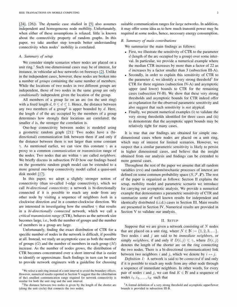
An example of a connected network is shown in Fig. 1

Fig. 1. An example of connected network.

When the network is connected, in order for packets fromnode i to reach node j, they have to follow a sequence ofintermediate nodes either in a clockwise direction or a counter-clockwise direction. In Fig. 1 packets from node i will followa counter-clockwise (resp. clockwise) route to node j (resp.node k). In some cases, however, the packets may be routedonly in one direction, but not in the other direction. When thishappens, the one-hop connectivity of nodes does not form acomplete ring and there is exactly one node that does not havea neighbor to its left (when all nodes are facing in the directionof the center of the disk). For instance, in Fig. 1 node k doesnot have a neighbor to its left and packets from node i cannotbe routed clockwise to node j.

We focus on the case where the one-hop connectivity of thenodes forms a complete ring. In other words, every node has aneighbor to its left and a packet generated by any node can berouted to any other node by traversing a sequence of intermedi-ate nodes both in clockwise and counter-clockwise directions.We call this bi-directional connectivity. It is obvious that thenetwork in Fig. 1 is not bi-directionally connected. In orderto distinguish from bi-directional connectivity, we refer to theconnectivity in Definition 1 as “usual” connectivity. Unlessstated otherwise, throughout the rest of the paper, networkconnectivity refers to bi-directional connectivity.

Obviously, bi-directional connectivity is a stronger conditionthan usual connectivity; bi-directional connectivity implies2-vertex connectivity and 2-edge connectivity [4]. In otherwords, the network would still be connected after removingany one node or a link in the network. Bi-directional con-nectivity and k-edge/vertex connectivity are studied in opticalnetworks [16] and in wireless sensor networks [15], [27]for fault tolerance. Numerical results in Section V indicatethat the smallest communication ranges needed for usualconnectivity and bi-directional connectivity on a unit ringdo not differ significantly for large networks. In addition,the distributions of such a minimum required communicationrange for bi-directional connectivity on a unit ring and forusual connectivity on a unit interval are very close.

A. Parametric scenario

Given a network with N ∈ IN nodes, the CTR of thenetwork, denoted by rc(N), is defined to be the smallestcommunication range4 of the nodes such that the networkis connected. Obviously, this CTR depends on the numberof nodes in the network, N , and their exact locations, andcomputing the exact distribution of the CTR is challenging.

For this reason, researchers often turn to an asymptotictheory for rc(N) as the number of nodes N becomes large:As mentioned in Section I, oftentimes, as the number of nodesgrows (while keeping other parameters fixed), the distributionof the CTR concentrates over a (short) interval we can identifyor approximate more easily. Following this spirit we areinterested in examining how γc(N) behaves as N increases.To this end, we introduce the following parametric scenario:

For each n ∈ IN, there are N(n) ≥ 1 nodes in the network.These N(n) nodes belong to G(n) groups with each groupconsisting of M(n) = N(n)/G(n) nodes, called the members.Let G(n) := 1, 2, . . . , G(n) denote the set of groups andM(n) := 1, 2, . . . ,M(n) the set of members in a group.We assume that as n → ∞, both the number of groups andthe number of members in a group increase unbounded, i.e.,G(n)→∞ and M(n)→∞.

1. Group mobility model – For each group k ∈ G(n),there is a virtual group leader (VGL) V (n)

k .5 This VGL movesaccording to some stochastic mobility process on the unitring. We denote the mobility process or trajectory of V (n)

k

by X(n)k := X(n)

k (t); t ∈ IR+, where IR+ := [0,∞) andX

(n)k (t) is the location of V (n)

k at time t. Here, X(n)k (t) ∈

[0, 1) denotes the length of the arc connecting some fixedreference point to V (n)

k , moving clockwise on the unit ring.The mobility process of the m-th node in the k-th group,

denoted by L(n)k,m := L(n)

k,m(t); t ∈ IR+, can be written as asum of two stochastic processes:6

L(n)k,m = X(n)

k +Y(n)k,m, (1)

where Y(n)k,m, k ∈ G(n) and m ∈ M(n), are identically dis-

tributed stochastic processes. We can interpret (1) as follows.While the process X(n)

k describes the movement of (the VGLfor) the group, the processes Y(n)

k,m determine the movementsof individual members in the group relative to the location ofVGL. Note that this model is similar to the reference pointgroup mobility model proposed in [14].

We consider the case where the movements of the membersare constrained to an arc near the VGL. More precisely, theprocess Y(n)

k,m := Y (n)k,m(t); t ∈ IR+ is limited to an interval

[0, d(n)] =: Dg with 0 ≤ d(n) ≤ 1, i.e., Y (n)k,m(t) ∈ Dg

for all t ∈ IR+. In this case the VGL is at the front ofthe group and the members follow the VGL, staying withind(n). However, Dg can be any interval of length d(n), e.g.,

4The communication range of a node is defined to be the maximum distanceanother node can be at, while maintaining a communication link with the node.

5The VGL V (n)k

is not a real node in the network. Instead, it is introducedto model the movement of the group.

6All additions are modulo one throughout the paper.

IEEE TRANSACTIONS ON MOBILE COMPUTING 4

[−d(n)/2, d(n)/2], without affecting the findings in thispaper.

We introduce the following assumptions on the mobilityprocesses:A1. The processes X(n)

k , k ∈ G(n), and Y(n)k,m, k ∈ G(n) and

m ∈M(n), are stationary and ergodic [8].A2. The processes X(n)

k , k ∈ G(n), are mutually independentand identically distributed. In addition, they yield aspatial distribution Fg with a continuous density fg :[0, 1) → IR+, which is uniform over the unit ring, i.e.,fg(x) = 1 for all x ∈ [0, 1).

A3. The processes Y(n)k,m, k ∈ G(n) and m ∈ M(n),

are mutually independent and are also independent ofX

(n)k , k ∈ G(n). Moreover, they yield a spatial distribu-

tion Fm (with density fm) uniform over the interval Dg

with fm(y) = 1/d(n) for all y ∈ Dg .

III. CONNECTIVITY OF STATIC GRAPHS

As mentioned earlier, in order for a network to be ableto provide an end-to-end route between arbitrary sources anddestinations (when a connection is requested), the networkshould be connected most of the time. From the assumedergodicity and stationarity of the mobility processes, thisimplies that the network sampled at some random time shouldbe connected with high probability.

Suppose that we sample the network at time ts ∈ IR+. Fromthe stated stationarity assumption, without loss of generality,we can assume ts = 0. Furthermore, for notational simplicitywe omit the dependence on time, e.g., we write X(n)

k in placeof X(n)

k (0). Under assumptions A1 through A3, we can makefollowing observations:O1. The rvs X(n)

k , k ∈ G(n), are independent and uniformlydistributed on the unit ring. Furthermore, L(n)

k,m, k ∈ G(n)

and m ∈ M(n), are uniformly distributed on the unitring. This is a consequence of the first observation thatX

(n)k is uniformly distributed on the unit ring and the

assumption that L(n)k,m is uniformly distributed on the

interval [X(n)k , X

(n)k + d(n)], no matter what the value

of X(n)k is.

O2. The locations of members in the same group, L(n)k,m, m ∈

M(n), are not mutually independent when d(n) < 1.However, given X(n)

k , k ∈ G(n), the rvs L(n)k,m, k ∈

G(n) and m ∈ M(n), are conditionally independent. Inparticular, for each k ∈ G(n), given X(n)

k , the locationsof the members in the k-th group, L(n)

k,m, m ∈ M(n),are conditionally independent rvs uniformly distributedon the arc [X(n)

k , X(n)k + d(n)].

We note that when d(n) = 1, the locations of all the nodesare independent and uniformly distributed on the unit ringregardless of Xk(n); k ∈ G(n) (so-called i.i.d. case). Onthe other hand, if d(n) is very small, the locations L(n)

k,m,m ∈M(n), are strongly correlated in that the members of a groupare very close to each other. In this sense, d(n) is used as aparameter to vary the degree of correlation in the locations ofthe members in a group.

Let G(G(n),M(n); γ) be the geometric random graphrepresenting the one-hop connectivity of the network withG(n) groups and M(n) members in each group (with a totalof N(n) = G(n) ×M(n) nodes), where each node employsa communication range of γ, according to the setup describedin the previous section. We define

P(n) (γ) := P [G(G(n),M(n); γ) is connected] .

It is obvious that P(n) (γ) is increasing in γ.

A. An example of parametric sensitivity and motivation

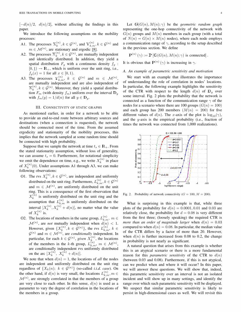
We start with an example that illustrates the importanceof understanding the role of correlation in nodes’ locations.In particular, the following example highlights the sensitivityof the CTR with respect to the length d(n) of Dg oversome interval. Fig. 2 plots the probability that the network isconnected as a function of the communication range γ of thenodes for a scenario where there are 100 groups (G(n) = 100)and each group has 200 members (M(n) = 200) for fivedifferent values of d(n). The x-axis of the plot is log10(γ),and the y-axis is the empirical probability (i.e., fraction oftimes the network was connected from 1,000 realizations).

Fig. 2. Probability of network connectivity (G = 100,M = 200).

What is surprising in this example is that, while threeplots of the probability for d(n) = 0.0001, 0.01 and 0.03 arerelatively close, the probability for d = 0.08 is very differentfrom the first three; (loosely speaking) the required CTR ismore than an order of magnitude larger when d(n) = 0.03compared to when d(n) = 0.08. In particular, the median valueof the CTR differs by a factor of more than 20. However,when d(n) is further increased from 0.08 to 0.2, the changein probability is not nearly as significant.

A natural question that arises from this example is whetherthis is an atypical scenario or there is a more fundamentalreason for this parametric sensitivity of the CTR to d(n)(between 0.03 and 0.08). Furthermore, if this is not atypical,can we predict when and where it will occur? In this paper,we will answer these questions. We will show that, indeed,this parametric sensitivity over an interval is not an isolatedincident and will show up in many settings, and identify therange over which such parametric sensitivity will be displayed.We suspect that similar parametric sensitivity is likely topersist in high-dimensional cases as well. We will revisit this

IEEE TRANSACTIONS ON MOBILE COMPUTING 5

example in subsection IV-C.

B. I.i.d. cases and (very) strong threshold

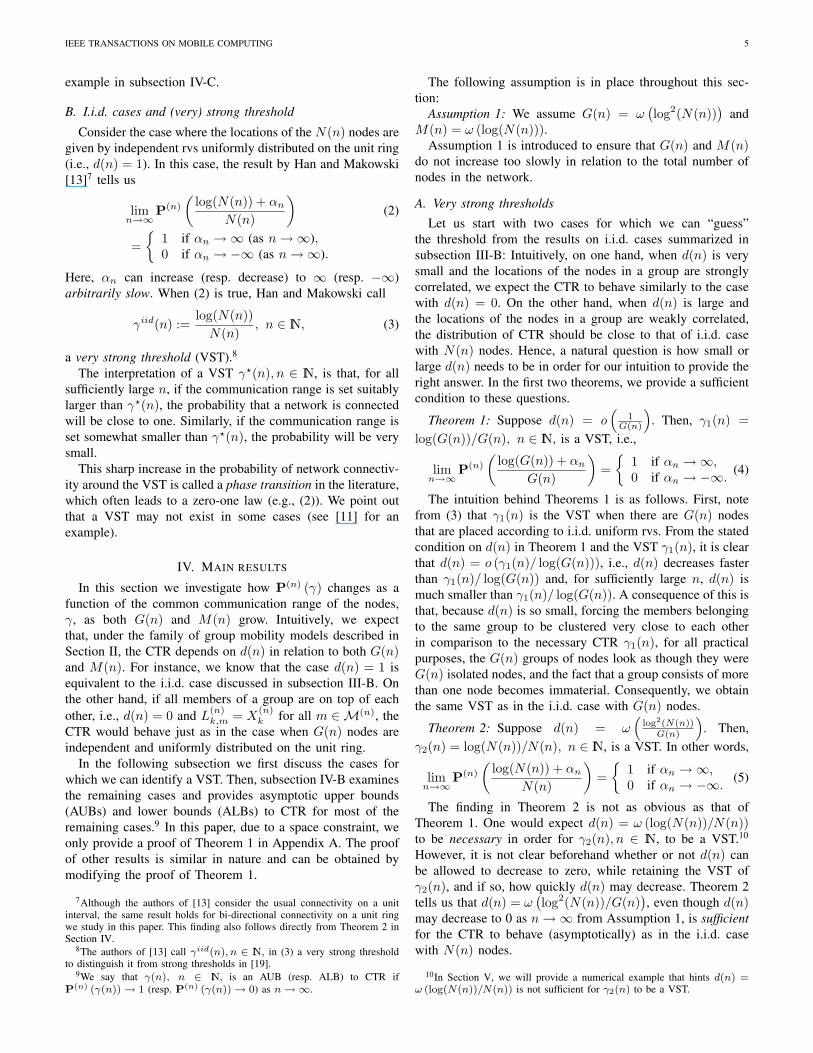
Consider the case where the locations of the N(n) nodes aregiven by independent rvs uniformly distributed on the unit ring(i.e., d(n) = 1). In this case, the result by Han and Makowski[13]7 tells us

limn→∞

P(n)

(log(N(n)) + αn

N(n)

)(2)

=

1 if αn →∞ (as n→∞),0 if αn → −∞ (as n→∞).

Here, αn can increase (resp. decrease) to ∞ (resp. −∞)arbitrarily slow. When (2) is true, Han and Makowski call

γiid(n) :=log(N(n))N(n)

, n ∈ IN, (3)

a very strong threshold (VST).8

The interpretation of a VST γ?(n), n ∈ IN, is that, for allsufficiently large n, if the communication range is set suitablylarger than γ?(n), the probability that a network is connectedwill be close to one. Similarly, if the communication range isset somewhat smaller than γ?(n), the probability will be verysmall.

This sharp increase in the probability of network connectiv-ity around the VST is called a phase transition in the literature,which often leads to a zero-one law (e.g., (2)). We point outthat a VST may not exist in some cases (see [11] for anexample).

IV. MAIN RESULTS

In this section we investigate how P(n) (γ) changes as afunction of the common communication range of the nodes,γ, as both G(n) and M(n) grow. Intuitively, we expectthat, under the family of group mobility models described inSection II, the CTR depends on d(n) in relation to both G(n)and M(n). For instance, we know that the case d(n) = 1 isequivalent to the i.i.d. case discussed in subsection III-B. Onthe other hand, if all members of a group are on top of eachother, i.e., d(n) = 0 and L(n)

k,m = X(n)k for all m ∈M(n), the

CTR would behave just as in the case when G(n) nodes areindependent and uniformly distributed on the unit ring.

In the following subsection we first discuss the cases forwhich we can identify a VST. Then, subsection IV-B examinesthe remaining cases and provides asymptotic upper bounds(AUBs) and lower bounds (ALBs) to CTR for most of theremaining cases.9 In this paper, due to a space constraint, weonly provide a proof of Theorem 1 in Appendix A. The proofof other results is similar in nature and can be obtained bymodifying the proof of Theorem 1.

7Although the authors of [13] consider the usual connectivity on a unitinterval, the same result holds for bi-directional connectivity on a unit ringwe study in this paper. This finding also follows directly from Theorem 2 inSection IV.

8The authors of [13] call γiid(n), n ∈ IN, in (3) a very strong thresholdto distinguish it from strong thresholds in [19].

9We say that γ(n), n ∈ IN, is an AUB (resp. ALB) to CTR ifP(n) (γ(n))→ 1 (resp. P(n) (γ(n))→ 0) as n→∞.

The following assumption is in place throughout this sec-tion:

Assumption 1: We assume G(n) = ω(log2(N(n))

)and

M(n) = ω (log(N(n))).Assumption 1 is introduced to ensure that G(n) and M(n)

do not increase too slowly in relation to the total number ofnodes in the network.

A. Very strong thresholds

Let us start with two cases for which we can “guess”the threshold from the results on i.i.d. cases summarized insubsection III-B: Intuitively, on one hand, when d(n) is verysmall and the locations of the nodes in a group are stronglycorrelated, we expect the CTR to behave similarly to the casewith d(n) = 0. On the other hand, when d(n) is large andthe locations of the nodes in a group are weakly correlated,the distribution of CTR should be close to that of i.i.d. casewith N(n) nodes. Hence, a natural question is how small orlarge d(n) needs to be in order for our intuition to provide theright answer. In the first two theorems, we provide a sufficientcondition to these questions.

Theorem 1: Suppose d(n) = o(

1G(n)

). Then, γ1(n) =

log(G(n))/G(n), n ∈ IN, is a VST, i.e.,

limn→∞

P(n)

(log(G(n)) + αn

G(n)

)=

1 if αn →∞,0 if αn → −∞.

(4)

The intuition behind Theorems 1 is as follows. First, notefrom (3) that γ1(n) is the VST when there are G(n) nodesthat are placed according to i.i.d. uniform rvs. From the statedcondition on d(n) in Theorem 1 and the VST γ1(n), it is clearthat d(n) = o (γ1(n)/ log(G(n))), i.e., d(n) decreases fasterthan γ1(n)/ log(G(n)) and, for sufficiently large n, d(n) ismuch smaller than γ1(n)/ log(G(n)). A consequence of this isthat, because d(n) is so small, forcing the members belongingto the same group to be clustered very close to each otherin comparison to the necessary CTR γ1(n), for all practicalpurposes, the G(n) groups of nodes look as though they wereG(n) isolated nodes, and the fact that a group consists of morethan one node becomes immaterial. Consequently, we obtainthe same VST as in the i.i.d. case with G(n) nodes.

Theorem 2: Suppose d(n) = ω(

log2(N(n))G(n)

). Then,

γ2(n) = log(N(n))/N(n), n ∈ IN, is a VST. In other words,

limn→∞

P(n)

(log(N(n)) + αn

N(n)

)=

1 if αn →∞,0 if αn → −∞.

(5)

The finding in Theorem 2 is not as obvious as that ofTheorem 1. One would expect d(n) = ω (log(N(n))/N(n))to be necessary in order for γ2(n), n ∈ IN, to be a VST.10

However, it is not clear beforehand whether or not d(n) canbe allowed to decrease to zero, while retaining the VST ofγ2(n), and if so, how quickly d(n) may decrease. Theorem 2tells us that d(n) = ω

(log2(N(n))/G(n)

), even though d(n)

may decrease to 0 as n→∞ from Assumption 1, is sufficientfor the CTR to behave (asymptotically) as in the i.i.d. casewith N(n) nodes.

10In Section V, we will provide a numerical example that hints d(n) =ω (log(N(n))/N(n)) is not sufficient for γ2(n) to be a VST.

IEEE TRANSACTIONS ON MOBILE COMPUTING 6

Fig. 3. Summary of results.

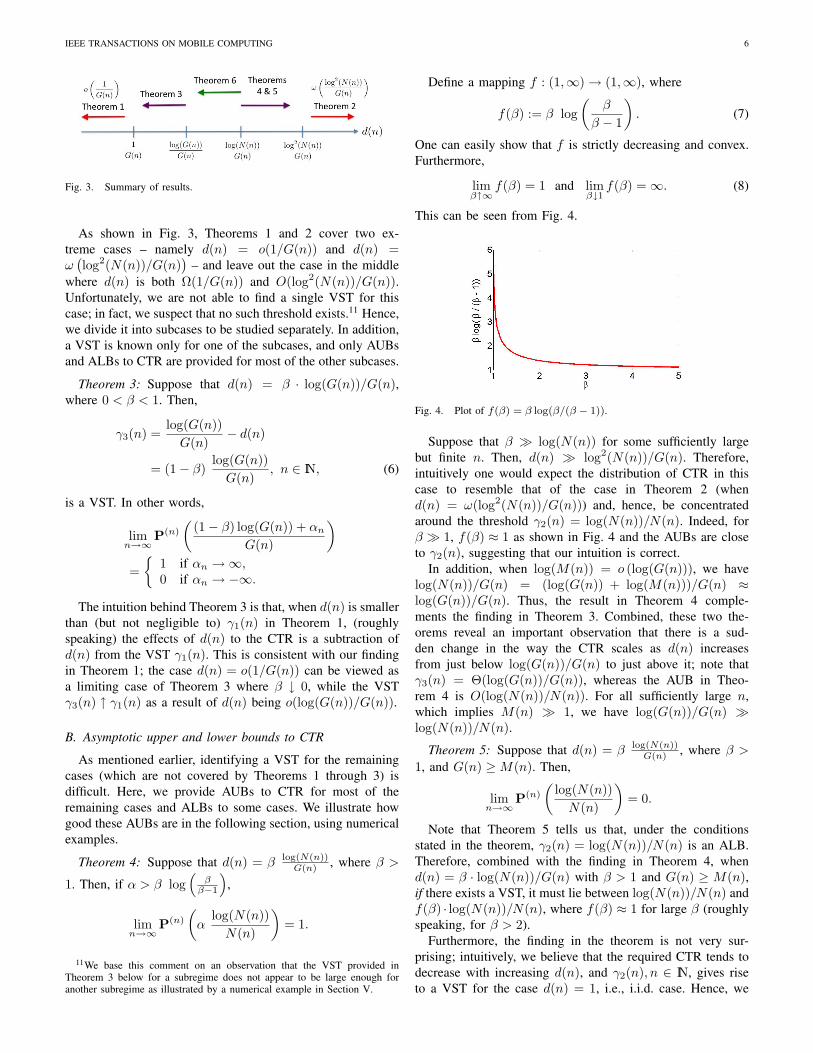
As shown in Fig. 3, Theorems 1 and 2 cover two ex-treme cases – namely d(n) = o(1/G(n)) and d(n) =ω(log2(N(n))/G(n)

)– and leave out the case in the middle

where d(n) is both Ω(1/G(n)) and O(log2(N(n))/G(n)).Unfortunately, we are not able to find a single VST for thiscase; in fact, we suspect that no such threshold exists.11 Hence,we divide it into subcases to be studied separately. In addition,a VST is known only for one of the subcases, and only AUBsand ALBs to CTR are provided for most of the other subcases.

Theorem 3: Suppose that d(n) = β · log(G(n))/G(n),where 0 < β < 1. Then,

γ3(n) =log(G(n))G(n)

− d(n)

= (1− β)log(G(n))G(n)

, n ∈ IN, (6)

is a VST. In other words,

limn→∞

P(n)

((1− β) log(G(n)) + αn

G(n)

)=

1 if αn →∞,0 if αn → −∞.

The intuition behind Theorem 3 is that, when d(n) is smallerthan (but not negligible to) γ1(n) in Theorem 1, (roughlyspeaking) the effects of d(n) to the CTR is a subtraction ofd(n) from the VST γ1(n). This is consistent with our findingin Theorem 1; the case d(n) = o(1/G(n)) can be viewed asa limiting case of Theorem 3 where β ↓ 0, while the VSTγ3(n) ↑ γ1(n) as a result of d(n) being o(log(G(n))/G(n)).

B. Asymptotic upper and lower bounds to CTR

As mentioned earlier, identifying a VST for the remainingcases (which are not covered by Theorems 1 through 3) isdifficult. Here, we provide AUBs to CTR for most of theremaining cases and ALBs to some cases. We illustrate howgood these AUBs are in the following section, using numericalexamples.

Theorem 4: Suppose that d(n) = β log(N(n))G(n) , where β >

1. Then, if α > β log(

ββ−1

),

limn→∞

P(n)

(α

log(N(n))N(n)

)= 1.

11We base this comment on an observation that the VST provided inTheorem 3 below for a subregime does not appear to be large enough foranother subregime as illustrated by a numerical example in Section V.

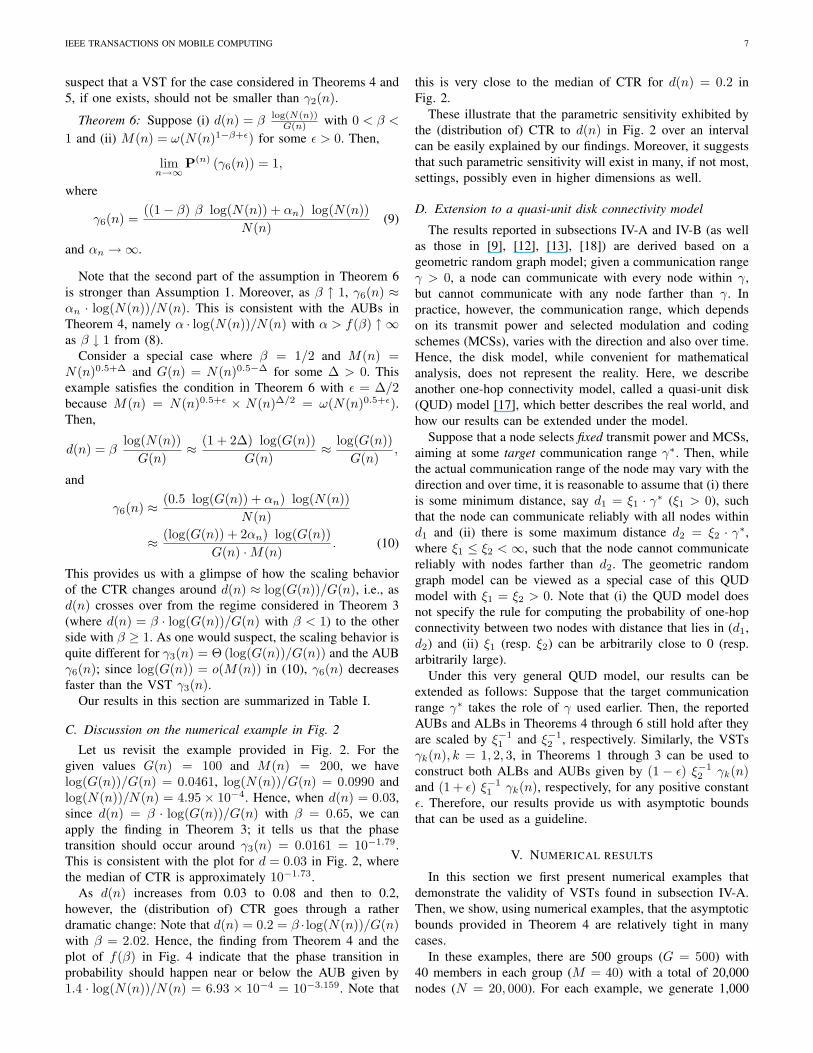
Define a mapping f : (1,∞)→ (1,∞), where

f(β) := β log(

β

β − 1

). (7)

One can easily show that f is strictly decreasing and convex.Furthermore,

limβ↑∞

f(β) = 1 and limβ↓1

f(β) =∞. (8)

This can be seen from Fig. 4.

Fig. 4. Plot of f(β) = β log(β/(β − 1)).

Suppose that β log(N(n)) for some sufficiently largebut finite n. Then, d(n) log2(N(n))/G(n). Therefore,intuitively one would expect the distribution of CTR in thiscase to resemble that of the case in Theorem 2 (whend(n) = ω(log2(N(n))/G(n))) and, hence, be concentratedaround the threshold γ2(n) = log(N(n))/N(n). Indeed, forβ 1, f(β) ≈ 1 as shown in Fig. 4 and the AUBs are closeto γ2(n), suggesting that our intuition is correct.

In addition, when log(M(n)) = o (log(G(n))), we havelog(N(n))/G(n) = (log(G(n)) + log(M(n)))/G(n) ≈log(G(n))/G(n). Thus, the result in Theorem 4 comple-ments the finding in Theorem 3. Combined, these two the-orems reveal an important observation that there is a sud-den change in the way the CTR scales as d(n) increasesfrom just below log(G(n))/G(n) to just above it; note thatγ3(n) = Θ(log(G(n))/G(n)), whereas the AUB in Theo-rem 4 is O(log(N(n))/N(n)). For all sufficiently large n,which implies M(n) 1, we have log(G(n))/G(n) log(N(n))/N(n).

Theorem 5: Suppose that d(n) = β log(N(n))G(n) , where β >

1, and G(n) ≥M(n). Then,

limn→∞

P(n)

(log(N(n))N(n)

)= 0.

Note that Theorem 5 tells us that, under the conditionsstated in the theorem, γ2(n) = log(N(n))/N(n) is an ALB.Therefore, combined with the finding in Theorem 4, whend(n) = β · log(N(n))/G(n) with β > 1 and G(n) ≥ M(n),if there exists a VST, it must lie between log(N(n))/N(n) andf(β) · log(N(n))/N(n), where f(β) ≈ 1 for large β (roughlyspeaking, for β > 2).

Furthermore, the finding in the theorem is not very sur-prising; intuitively, we believe that the required CTR tends todecrease with increasing d(n), and γ2(n), n ∈ IN, gives riseto a VST for the case d(n) = 1, i.e., i.i.d. case. Hence, we

IEEE TRANSACTIONS ON MOBILE COMPUTING 7

suspect that a VST for the case considered in Theorems 4 and5, if one exists, should not be smaller than γ2(n).

Theorem 6: Suppose (i) d(n) = β log(N(n))G(n) with 0 < β <

1 and (ii) M(n) = ω(N(n)1−β+ε) for some ε > 0. Then,

limn→∞

P(n) (γ6(n)) = 1,

where

γ6(n) =((1− β) β log(N(n)) + αn) log(N(n))

N(n)(9)

and αn →∞.

Note that the second part of the assumption in Theorem 6is stronger than Assumption 1. Moreover, as β ↑ 1, γ6(n) ≈αn · log(N(n))/N(n). This is consistent with the AUBs inTheorem 4, namely α · log(N(n))/N(n) with α > f(β) ↑ ∞as β ↓ 1 from (8).

Consider a special case where β = 1/2 and M(n) =N(n)0.5+∆ and G(n) = N(n)0.5−∆ for some ∆ > 0. Thisexample satisfies the condition in Theorem 6 with ε = ∆/2because M(n) = N(n)0.5+ε × N(n)∆/2 = ω(N(n)0.5+ε).Then,

d(n) = βlog(N(n))G(n)

≈ (1 + 2∆) log(G(n))G(n)

≈ log(G(n))G(n)

,

and

γ6(n) ≈ (0.5 log(G(n)) + αn) log(N(n))N(n)

≈ (log(G(n)) + 2αn) log(G(n))G(n) ·M(n)

. (10)

This provides us with a glimpse of how the scaling behaviorof the CTR changes around d(n) ≈ log(G(n))/G(n), i.e., asd(n) crosses over from the regime considered in Theorem 3(where d(n) = β · log(G(n))/G(n) with β < 1) to the otherside with β ≥ 1. As one would suspect, the scaling behavior isquite different for γ3(n) = Θ (log(G(n))/G(n)) and the AUBγ6(n); since log(G(n)) = o(M(n)) in (10), γ6(n) decreasesfaster than the VST γ3(n).

Our results in this section are summarized in Table I.

C. Discussion on the numerical example in Fig. 2

Let us revisit the example provided in Fig. 2. For thegiven values G(n) = 100 and M(n) = 200, we havelog(G(n))/G(n) = 0.0461, log(N(n))/G(n) = 0.0990 andlog(N(n))/N(n) = 4.95× 10−4. Hence, when d(n) = 0.03,since d(n) = β · log(G(n))/G(n) with β = 0.65, we canapply the finding in Theorem 3; it tells us that the phasetransition should occur around γ3(n) = 0.0161 = 10−1.79.This is consistent with the plot for d = 0.03 in Fig. 2, wherethe median of CTR is approximately 10−1.73.

As d(n) increases from 0.03 to 0.08 and then to 0.2,however, the (distribution of) CTR goes through a ratherdramatic change: Note that d(n) = 0.2 = β · log(N(n))/G(n)with β = 2.02. Hence, the finding from Theorem 4 and theplot of f(β) in Fig. 4 indicate that the phase transition inprobability should happen near or below the AUB given by1.4 · log(N(n))/N(n) = 6.93 × 10−4 = 10−3.159. Note that

this is very close to the median of CTR for d(n) = 0.2 inFig. 2.

These illustrate that the parametric sensitivity exhibited bythe (distribution of) CTR to d(n) in Fig. 2 over an intervalcan be easily explained by our findings. Moreover, it suggeststhat such parametric sensitivity will exist in many, if not most,settings, possibly even in higher dimensions as well.

D. Extension to a quasi-unit disk connectivity model

The results reported in subsections IV-A and IV-B (as wellas those in [9], [12], [13], [18]) are derived based on ageometric random graph model; given a communication rangeγ > 0, a node can communicate with every node within γ,but cannot communicate with any node farther than γ. Inpractice, however, the communication range, which dependson its transmit power and selected modulation and codingschemes (MCSs), varies with the direction and also over time.Hence, the disk model, while convenient for mathematicalanalysis, does not represent the reality. Here, we describeanother one-hop connectivity model, called a quasi-unit disk(QUD) model [17], which better describes the real world, andhow our results can be extended under the model.

Suppose that a node selects fixed transmit power and MCSs,aiming at some target communication range γ∗. Then, whilethe actual communication range of the node may vary with thedirection and over time, it is reasonable to assume that (i) thereis some minimum distance, say d1 = ξ1 · γ∗ (ξ1 > 0), suchthat the node can communicate reliably with all nodes withind1 and (ii) there is some maximum distance d2 = ξ2 · γ∗,where ξ1 ≤ ξ2 <∞, such that the node cannot communicatereliably with nodes farther than d2. The geometric randomgraph model can be viewed as a special case of this QUDmodel with ξ1 = ξ2 > 0. Note that (i) the QUD model doesnot specify the rule for computing the probability of one-hopconnectivity between two nodes with distance that lies in (d1,d2) and (ii) ξ1 (resp. ξ2) can be arbitrarily close to 0 (resp.arbitrarily large).

Under this very general QUD model, our results can beextended as follows: Suppose that the target communicationrange γ∗ takes the role of γ used earlier. Then, the reportedAUBs and ALBs in Theorems 4 through 6 still hold after theyare scaled by ξ−1

1 and ξ−12 , respectively. Similarly, the VSTs

γk(n), k = 1, 2, 3, in Theorems 1 through 3 can be used toconstruct both ALBs and AUBs given by (1 − ε) ξ−1

2 γk(n)and (1 + ε) ξ−1

1 γk(n), respectively, for any positive constantε. Therefore, our results provide us with asymptotic boundsthat can be used as a guideline.

V. NUMERICAL RESULTS

In this section we first present numerical examples thatdemonstrate the validity of VSTs found in subsection IV-A.Then, we show, using numerical examples, that the asymptoticbounds provided in Theorem 4 are relatively tight in manycases.

In these examples, there are 500 groups (G = 500) with40 members in each group (M = 40) with a total of 20,000nodes (N = 20, 000). For each example, we generate 1,000

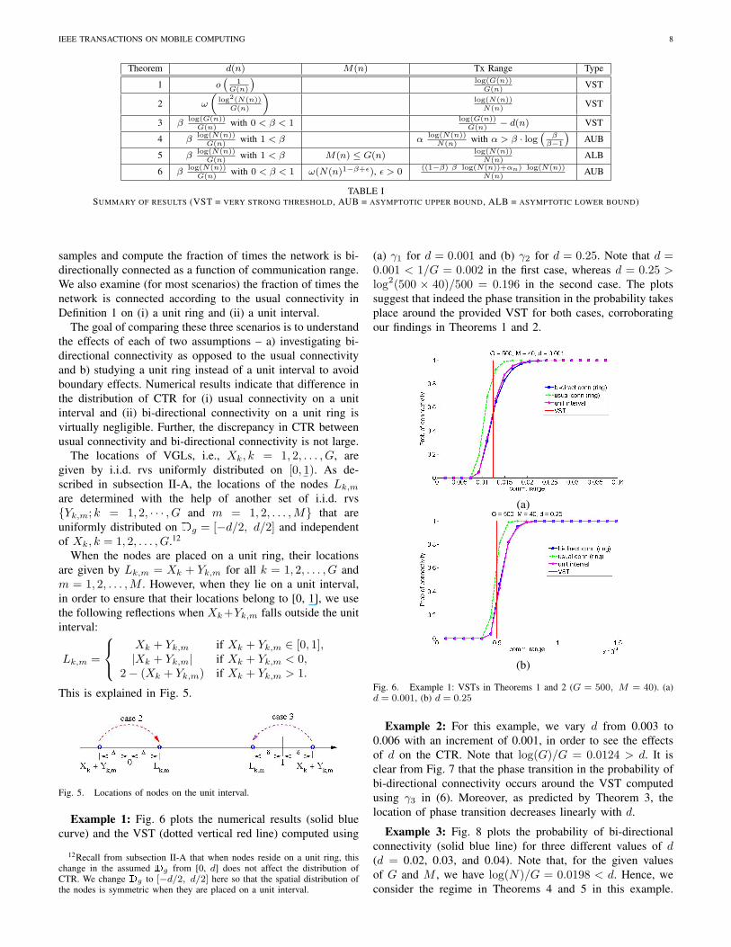
IEEE TRANSACTIONS ON MOBILE COMPUTING 8

Theorem d(n) M(n) Tx Range Type

1 o(

1G(n)

)log(G(n))G(n)

VST

2 ω

(log2(N(n))

G(n)

)log(N(n))N(n)

VST

3 βlog(G(n))G(n)

with 0 < β < 1log(G(n))G(n)

− d(n) VST

4 βlog(N(n))G(n)

with 1 < β αlog(N(n))N(n)

with α > β · log(

ββ−1

)AUB

5 βlog(N(n))G(n)

with 1 < β M(n) ≤ G(n)log(N(n))N(n)

ALB

6 βlog(N(n))G(n)

with 0 < β < 1 ω(N(n)1−β+ε), ε > 0((1−β) β log(N(n))+αn) log(N(n))

N(n)AUB

TABLE ISUMMARY OF RESULTS (VST = VERY STRONG THRESHOLD, AUB = ASYMPTOTIC UPPER BOUND, ALB = ASYMPTOTIC LOWER BOUND)

samples and compute the fraction of times the network is bi-directionally connected as a function of communication range.We also examine (for most scenarios) the fraction of times thenetwork is connected according to the usual connectivity inDefinition 1 on (i) a unit ring and (ii) a unit interval.

The goal of comparing these three scenarios is to understandthe effects of each of two assumptions – a) investigating bi-directional connectivity as opposed to the usual connectivityand b) studying a unit ring instead of a unit interval to avoidboundary effects. Numerical results indicate that difference inthe distribution of CTR for (i) usual connectivity on a unitinterval and (ii) bi-directional connectivity on a unit ring isvirtually negligible. Further, the discrepancy in CTR betweenusual connectivity and bi-directional connectivity is not large.

The locations of VGLs, i.e., Xk, k = 1, 2, . . . , G, aregiven by i.i.d. rvs uniformly distributed on [0, 1). As de-scribed in subsection II-A, the locations of the nodes Lk,mare determined with the help of another set of i.i.d. rvsYk,m; k = 1, 2, · · · , G and m = 1, 2, . . . ,M that areuniformly distributed on Dg = [−d/2, d/2] and independentof Xk, k = 1, 2, . . . , G.12

When the nodes are placed on a unit ring, their locationsare given by Lk,m = Xk + Yk,m for all k = 1, 2, . . . , G andm = 1, 2, . . . ,M . However, when they lie on a unit interval,in order to ensure that their locations belong to [0, 1], we usethe following reflections when Xk+Yk,m falls outside the unitinterval:

Lk,m =

Xk + Yk,m if Xk + Yk,m ∈ [0, 1],|Xk + Yk,m| if Xk + Yk,m < 0,

2− (Xk + Yk,m) if Xk + Yk,m > 1.

This is explained in Fig. 5.

Fig. 5. Locations of nodes on the unit interval.

Example 1: Fig. 6 plots the numerical results (solid bluecurve) and the VST (dotted vertical red line) computed using

12Recall from subsection II-A that when nodes reside on a unit ring, thischange in the assumed Dg from [0, d] does not affect the distribution ofCTR. We change Dg to [−d/2, d/2] here so that the spatial distribution ofthe nodes is symmetric when they are placed on a unit interval.

(a) γ1 for d = 0.001 and (b) γ2 for d = 0.25. Note that d =0.001 < 1/G = 0.002 in the first case, whereas d = 0.25 >log2(500 × 40)/500 = 0.196 in the second case. The plotssuggest that indeed the phase transition in the probability takesplace around the provided VST for both cases, corroboratingour findings in Theorems 1 and 2.

(a)

(b)

Fig. 6. Example 1: VSTs in Theorems 1 and 2 (G = 500, M = 40). (a)d = 0.001, (b) d = 0.25

Example 2: For this example, we vary d from 0.003 to0.006 with an increment of 0.001, in order to see the effectsof d on the CTR. Note that log(G)/G = 0.0124 > d. It isclear from Fig. 7 that the phase transition in the probability ofbi-directional connectivity occurs around the VST computedusing γ3 in (6). Moreover, as predicted by Theorem 3, thelocation of phase transition decreases linearly with d.

Example 3: Fig. 8 plots the probability of bi-directionalconnectivity (solid blue line) for three different values of d(d = 0.02, 0.03, and 0.04). Note that, for the given valuesof G and M , we have log(N)/G = 0.0198 < d. Hence, weconsider the regime in Theorems 4 and 5 in this example.

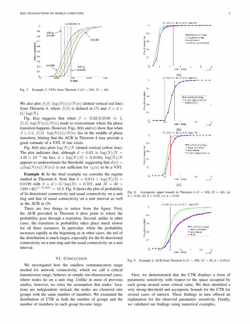
IEEE TRANSACTIONS ON MOBILE COMPUTING 9

Fig. 7. Example 2: VSTs from Theorem 3 (G = 500,M = 40).

We also plot f(β) · log(N(n))/N(n) (dotted vertical red line)from Theorem 4, where f(β) is defined in (7) and β = d ×G/ log(N).

Fig. 8(a) suggests that when β = 0.02/0.0198 ≈ 1,f(β) · log(N(n))/N(n) tends to overestimate where the phasetransition happens. However, Figs. 8(b) and (c) show that whenβ > 1.5, f(β) · log(N(n))/N(n) lies in the middle of phasetransition, hinting that the AUB in Theorem 4 may provide agood estimate of a VST, if one exists.

Fig. 8(b) also plots log(N)/N (dotted vertical yellow line).The plot indicates that, although d = 0.03 log(N)/N =4.95 × 10−4 (in fact, d > log(N)/G = 0.0198), log(N)/Nappears to underestimate the threshold, suggesting that d(n) =ω(log(N(n))/N(n)) is not sufficient for γ2(n) to be a VST.

Example 4: In the final example we consider the regimestudied in Theorem 6. Note that d = 0.014 < log(N)/G =0.0198 with β = d × G/ log(N) = 0.707, and M = 40 >(500×40)(1−0.707) = 18.2. Fig. 9 shows the plot of probabilityof bi-directional connectivity and usual connectivity on a unitring and that of usual connectivity on a unit interval as wellas the AUB in (9).

There are two things to notice from the figure. First,the AUB provided in Theorem 6 does point to where theprobability goes through a transition. Second, unlike in othercases, the transition in probability takes place much slowerfor all three scenarios. In particular, while the probabilityincreases rapidly at the beginning as in other cases, the tail ofthe distribution is much larger, especially for the bi-directionalconnectivity on a unit ring and the usual connectivity on a unitinterval.

VI. CONCLUSION

We investigated how the smallest communication rangeneeded for network connectivity, which we call a criticaltransmission range, behaves in simple one-dimensional cases,where nodes lie on a unit ring. Unlike in most of previousstudies, however, we relax the assumption that nodes’ loca-tions are independent; instead, the nodes are clustered intogroups with the same number of members. We examined thedistribution of CTR as both the number of groups and thenumber of members in each group become large.

(a)

(b)

(c)

Fig. 8. Asymptotic upper bounds in Theorem 4 (G = 500,M = 40). (a)d = 0.02, (b) d = 0.03, (c) d = 0.04.

Fig. 9. Example 2: AUB from Theorem 6 (G = 500,M = 40, d = 0.014).

First, we demonstrated that the CTR displays a form ofparametric sensitivity with respect to the space occupied byeach group around some critical value. We then identified avery strong threshold and asymptotic bounds for the CTR forseveral cases of interest. These findings in turn offered anexplanation for the observed parametric sensitivity. Finally,we validated our findings using numerical examples.

IEEE TRANSACTIONS ON MOBILE COMPUTING 10

While we focused on a simple one-dimensional case asa first step towards understanding the role of correlation innodes’ locations on network connectivity, we suspect that aparametric sensitivity similar to the one we observed in one-dimensional cases persists in higher-dimensional cases.

REFERENCES

[1] M. J. B. Appel and R. P. Russo, “The connectivity of a graph on uniformpoints on [0, 1]d,” Statistics & Probability Letters, 60:351-357, 2002.

[2] F. Bai, N. Sadagopan and A. Helmy, “IMPORTANT: A framework tosystematically analyze the impact of mobility on performance of routingprotocols for adhoc networks,” in Proceedings of IEEE INFOCOM, SanFrancisco (CA), Mar. 2003.

[3] C. Bettstetter, “Mobility modeling in wireless networks: categorization,smooth movement, border effects,” ACM Mobile Computing and Com-munications Review, 5(3): 55-67, Jul. 2001.

[4] B. Bollobas, Modern Graph Theory, Springer-Verlag, 1998.[5] J. Diaz, D. Mitsche and X. Perez-Gimenez, “Large connectivity for

dynamic random geometric graphs,” IEEE Trans. on Mobile Computing(TMC), 8(6):821-835, Jun. 2009.

[6] P. Erdos and A. Renyi, “On random graphs. I,” Publicationes Mathe-maticae, 6: 290-297, 1959.

[7] P. Erdos and A. Renyi, “The evolution of random graphs”. Magyar Tud.Akad. Mat. Kutato Int. Kozl., 5:17-61, 1960.

[8] G. Grimmett and D. Stirzaker, Probability and Random Processes, thirded., Oxford University Press, 2001.

[9] P. Gupta and P. R. Kumar, “Critical power for asymptotic connectivityin wireless networks,” Stochastic Analysis, Control, and Optimizationand Applications, pp. 547-566, 1998.

[10] P. Gupta and P. R. Kumar, “The capacity of wireless networks,” IEEETrans. on Information Theory, 46(2):388-404, Mar. 2000.

[11] G. Han, “Connectivity analysis of wireless ad-hoc networks,” Ph.Ddissertation, Department of Electrical and Computer Engineering, Uni-versity of Maryland, College Park, 2007.

[12] G. Han and A. M. Makowski, “Very sharp transitions in one-dimensionalMANETs,” in Proceedings of 2006 IEEE International Conference onCommunications, vol. 1, pp. 217-222, Jun. 2006.

[13] G. Han and A. M. Makowski, “A very strong zero-one law for connec-tivity in one-dimensional geometric random graphs,” IEEE Communi-cations Letters, 11(1):55-57, Jan. 2007.

[14] X. Hong, M. Gerla, G. Pei and C. C. Chiang, “A group mobility modelfor ad hoc wireless networks,” in Proceedings of the 2nd ACM Inter-national Workshop on Modeling, Analysis and Simulation of Wirelessand Mobile Systems (MSWiM), pp. 53-60, Aug. 1999.

[15] A. Kashyap, S. Khuller, and M. Shayman,“Relay placement for higherorder connectivity in wireless sensor networks,” in Proc. IEEE INFO-COM 2006, pp. 1-12.

[16] C. H. Kim, C.-H. Lee and Y. C. Chung, “Bidirectional WDM self-healing ring network based on simple bidirectional add/drop amplifiermodules,” IEEE Photonics Technology Letters, 10(9):1340-1342, Sep.1998.

[17] F. Kuhn, R. Wattenhofer, and A. Zollinger, “Ad-hoc networks beyondunit disk graphs,” Wireless Networks, 14(5):715-729, Jul. 2007.

[18] S. S. Kunniyur and S. S. Venkatesh, “Connectivity, devolution, andlacunae in geometric random digraphs,” in Proceedings of the Workshopon Information Theory and Applications, Feb. 2006.

[19] G. L. McColm, “Threshold functions for random graphs on a linesegment,” Combinatorics, Probability and Computing, 13(3):373-387,May 2004.

[20] P. Nain, D. Towsley, B. Liu and Z. Liu, “Properties of random directionmodels,” in Proceedings of IEEE INFOCOM, Miami (FL), Mar. 2005.

[21] M. D. Penrose, Random Geometric Graphs, Oxford Studies in Proba-bility, Oxford University Press, 2003.

[22] M. D. Penrose, “A strong law for the longest edge of the minimalspanning tree,” The Annals of Probability, 27(1):246-260, 1999.

[23] T. S. Rappaport, Wireless Communications: Principles and Practice, 2ndEd., Prentice Hall PTR, 2002.

[24] P. Santi, “The critical transmitting range for connectivity in mobilead hoc networks,” IEEE Trans. on Mobile Computing, 4(3):310-317,May/June 2005.

[25] C. Scheideler, A. W. Richa, and P. Santi, “An O(log n) dominating setprotocol for wireless ad-hoc networks under the physical interferencemodel,” in Proceedings of the 9th ACM International Symposium onMobile Ad-hoc Networking and Computing, pp. 91-100, 2008.

[26] S. S. Venkatesh, “Connectivity of metric randomgraphs,” preprint, available at http://www.seas.upenn.edu/∼venkates/publications chronological.html

[27] H. Zhang and J. C. Hou, “Asymptotic critical total power for k-connectivity of wireless networks,” IEEE/ACM Trans. on Networking,16(2):347-358, Apr. 2008.

APPENDIX APROOF OF THEOREM 1

We first introduce some notation and preliminary results thatwill be used to prove the theorem. If node j lies within thecommunication range to the left of node i (when facing in thedirection of the center of the unit ring), we call node j a leftneighbor (LN) of node i. With a little abuse of notation, foreach n ∈ IN (and fixed G(n), M(n) and d(n)),

• I(n)k,m(γ), k ∈ G(n) and m ∈ M(n), is the indicator

function of the event that node m in the k-th group doesnot have any LNs on the unit ring; and

• C(n)(γ) =∑k∈G(n) C

(n)k (γ) denotes the total num-

ber of nodes without any LN, where C(n)k (γ) =∑

m∈M(n) I(n)k,m(γ).

Note that, according to these definitions, the event that therandom graphG(G(n),M(n); γ) is bi-directionally connectedis the same as the event C(n)(γ) = 0, and P(n) (γ) =P[C(n)(γ) = 0

]. Throughout the proof we will make use

of this equality and investigate P[C(n)(γ) = 0

]in place of

P(n)(γ).We borrow following results from [11] to simplify the proof

of the theorem: Define Z+ := 0, 1, 2, . . . to be the setof non-negative integers. Suppose Zn;n = 1, 2, · · · is asequence of Z+-valued rvs with finite second moment, i.e.,E[Z2n

]<∞, for every n = 1, 2, . . .. Then,

limn→∞

P [Zn = 0] = 1 if limn→∞

E [Zn] = 0, (11)

and

limn→∞

P [Zn = 0] = 0 if limn→∞

(E [Zn])2

E [Z2n]

= 1. (12)

Eq. (11) follows directly from Markov’s inequality [8, p.311].Eq. (12) can be easily shown using Cauchy-Schwarz inequal-ity [8, p.65].

We now return to the proof of Theorem 1 and define

γ(n) :=log(G(n)) + αn

G(n).

Here, when αn increases (resp. decreases), it increases (resp.decreases) to∞ (resp. −∞) arbitrarily slow. In order to proveTheorem 1, we will first show

S1. E[C(n)(γ(n))

]→ 0 if αn →∞, and

S2. (E[C(n)(γ(n))])2

E[(C(n)(γ(n)))2

] → 1 if αn → −∞,

and then make use of (11) and (12), respectively.Proof of S1: From the definition of C(n)(γ),

E[C(n)(γ(n))

]= N(n) ·E

[I

(n)1,1 (γ(n))

], (13)

IEEE TRANSACTIONS ON MOBILE COMPUTING 11

and we focus on computing E[I

(n)1,1 (γ(n))

]. Without loss of

generality (WLOG), suppose that the location of VGL V(n)1

is X(n)1 = 0 and, hence, L(n)

1,1 = Y(n)1,1 .

We denote the m-th node in the k-th group by the pair (k,m). Define event A(n) (resp. B(n)) to be the event that node(1, 1) has no LNs from group 1 (resp. from the other groups2 through G(n)). Then,

E[I

(n)1,1 (γ(n))

]= E

[E[I

(n)1,1 (γ(n))

∣∣∣ Y (n)1,1

]]=

1d(n)

∫ d(n)

0

(P

[A(n)

∣∣∣ y] ·P [B(n)∣∣∣ y]) dy

=P[B(n)

]d(n)

∫ d(n)

0

P

[A(n)

∣∣∣ y] dy, (14)

where P[A(n) | y

]and P

[B(n) | y

]are the conditional prob-

ability of A(n) and B(n), respectively, given Y (n)1,1 = y,13

and the second and third equalities follow from AssumptionsA1 and A2 in subsection II-A.

First, since d(n) < γ(n), it is easy to see that, givenY

(n)1,1 = y, in order for the event A(n) to be true, the other

members in group 1 must lie in [0, y). Hence, P[A(n)|y

]=

(y/d(n))M(n)−1 for all y ∈ [0, d(n)], and

1d(n)

∫ d(n)

0

P

[A(n)

∣∣∣ y] dy =1

M(n). (15)

Second, let B(n)2 be the event that node (1,1) does not have

any LNs from group 2. Then, from Assumptions A1 through

A3, P[B(n)

]=(P

[B

(n)2

])G(n)−1

. We compute P[B

(n)2

]by conditioning on X(n)

2 = x2 and considering four cases asfollows. WLOG, we assume L(n)

1,1 = 0:

Case 1. 0 ≤ x2 ≤ γ(n)− d(n) : The members of group 2will lie in the interval [x2, x2+d(n)], where x2+d(n) ≤ γ(n).Thus, because [x2, x2 +d(n)] ⊂ [0, γ(n)], they will be all LNsof node (1,1), and P

[B

(n)2 |X

(n)2 = x2

]= 0.

Case 2. γ(n) − d(n) < x2 ≤ γ(n) : The conditionalprobability P

[B

(n)2 |X

(n)2 = x2

]is given by the probability

that all members of group 2 are in the interval (γ(n), x2 +d(n)). From Assumption A3, this probability is given by((x2 + d(n)− γ(n))/d(n))M(n).

Case 3. γ(n) < x2 < 1−d(n) : Since all members of group2 lie in the interval (γ(n), 1), P

[B

(n)2 |X

(n)2 = x2

]= 1.

Case 4. 1 − d(n) ≤ x2 < 1 : The conditional probabilityP

[B

(n)2 |X

(n)2 = x2

]is equal to the probability that all mem-

bers in group 2 reside in (x2, 1). This probability is given by((1− x2)/d(n))M(n).

13One should view these conditional probabilities as the limit of

P

[A(n) | y < Y

(n)1,1 ≤ y + δ

]and P

[B(n) | y < Y

(n)1,1 ≤ y + δ

]when

δ → 0.

Integrating the above conditional probabilities over thecorresponding intervals, we get

P

[B

(n)2

]=∫ γ(n)

γ(n)−d(n)

(x2 + d(n)− γ(n)

d(n)

)M(n)

dx2

+∫ 1−d(n)

γ(n)

1 dx2 +∫ 1

1−d(n)

(1− x2

d(n)

)M(n)

dx2

= 1− γ(n)− M(n)− 1M(n) + 1

d(n). (16)

Recall that X(n)2 is uniformly distributed over [0, 1) from

observation O1 (in Section III).

From the equality P[B(n)

]=(P

[B

(n)2

])G(n)−1

and (16),

P

[B(n)

]=(

1− γ(n)− M(n)− 1M(n) + 1

d(n))G(n)−1

(17)

= exp(

(G(n)− 1) · log(

1− γ(n)− M(n)− 1M(n) + 1

d(n)))

.

Define Γ(n) := γ(n)+M(n)−1M(n)+1d(n). Then, because Γ(n)→ 0,

we have log(1− Γ(n)) = −Γ(n) +O(Γ(n)2

)and

P

[B(n)

]= exp

((G(n)− 1) ·

(−Γ(n) +O

(Γ(n)2

))).

First, note that G(n) ·d(n) = o(1) and G(n) · γ(n)2 = o(1)because G(n) = ω(log2(N(n))) from Assumption 1. Hence,G(n) · Γ(n)2 = o(1) because d(n) = o(γ(n)). Therefore,

P

[B(n)

]∼ exp(−G(n) · γ(n))

= exp (− (log(G(n)) + αn))

=1

G(n)exp(−αn). (18)

From (14), (15), and (18),

E[I

(n)1,1 (γ(n))

]∼ 1M(n)

× 1G(n)

exp(−αn)

=1

N(n)exp(−αn). (19)

Substituting (19) in (13), we obtain

E[C(n)(γ(n))

]= N(n) ·E

[I

(n)1,1 (γ(n))

]∼ N(n) · 1

N(n)exp(−αn)

= exp(−αn). (20)

Therefore, if αn →∞, E[C(n)(γ(n))

]→ 0. This completes

the proof of S1.

Proof of S2: First, from the definition of C(n)(γ(n)),

E[(C(n)(γ(n))

)2]

= E

G(n)∑k=1

C(n)k (γ(n))

2

= G(n) E[(C

(n)1 (γ(n))

)2]

+G(n)(G(n)− 1) E[C

(n)1 (γ(n)) · C(n)

2 (γ(n))],(21)

IEEE TRANSACTIONS ON MOBILE COMPUTING 12

where the second equality follows from the fact thatC

(n)k , k ∈ G(n), are exchangeable. Substituting C(n)

k (γ(n)) =∑M(n)m=1 I

(n)k,m(γ(n)) and expanding them out,

E[(C

(n)1 (γ(n))

)2]

= E

∑m∈M(n)

(I

(n)1,m(γ(n))

)2

+∑

m∈M(n)

∑m∗∈M(n)\m

I(n)1,m(γ(n)) · I(n)

1,m∗(γ(n))

= M(n) E

[I

(n)1,1 (γ(n))

](22)

+M(n) (M(n)− 1) E[I

(n)1,1 (γ(n)) · I(n)

1,2 (γ(n))]

and

E[C

(n)1 (γ(n)) · C(n)

2 (γ(n))]

= E

∑m∈M(n)

I(n)1,m(γ(n))

∑m∗∈M(n)

I(n)2,m∗(γ(n))

= M(n)2 E

[I

(n)1,1 (γ(n)) · I(n)

2,1 (γ(n))]. (23)

Plugging in (22) and (23) in (21), we obtain

E[(C(n)(γ(n))

)2]

= N(n) E[I

(n)1,1 (γ(n))

](24)

+N(n)(M(n)− 1) E[I

(n)1,1 (γ(n)) · I(n)

1,2 (γ(n))]

+N(n)M(n)(G(n)− 1) E[I

(n)1,1 (γ(n)) · I(n)

2,1 (γ(n))].

Recall that we already computed E[I

(n)1,1,(γ(n))

]and

E[C(n)(γ(n))

]in the proof of S1. Hence, in order to prove S2

using (24), we need to calculate E[I

(n)1,1 (γ(n)) · I(n)

1,2 (γ(n))]

and E[I

(n)1,1 (γ(n)) · I(n)

2,1 (γ(n))]. However, γ(n) > d(n)

immediately tells us that E[I

(n)1,1 (γ(n)) · I(n)

1,2 (γ(n))]

= 0because the two nodes are always within γ(n) of each other(and, hence, one of them is a LN of the other). Thus, we onlyneed to compute E

[I

(n)1,1 (γ(n)) · I(n)

2,1 (γ(n))].

Computation of E[I

(n)1,1 (γ(n)) · I(n)

2,1 (γ(n))]: Define Q(n)

(resp. R(n)) to be the event that no node from groups 1 and 2(resp. from groups 3 through G(n)) is a LN of node (1,1) or(2,1). WLOG we assume that node (1,1) is at L(n)

1,1 = 0. Then,by conditioning on the location of node (2,1), L(n)

2,1 = `2, andusing observation O1 (in Section III) that L(n)

2,1 is uniformlydistributed over [0, 1), we can write

E[I

(n)1,1 (γ(n)) · I(n)

2,1 (γ(n))]

=∫ 1

0

(P

[R(n)|`2

]·P[Q(n)|`2

])d`2, (25)

where P[R(n) | `2

]and P

[Q(n) | `2

]are the condi-

tional probabilities of R(n) and Q(n), respectively, given

L(n)2,1 = `2. We will now identify an upper bound for

E[I

(n)1,1 (γ(n)) · I(n)

2,1 (γ(n))]

by finding an upper bound to

P[Q(n) | `2

]and P

[R(n) | `2

].

(i) Upper bound for P[Q(n) | `2

]– First, note that if

`2 ∈ [1− γ(n), γ(n)], nodes (1,1) and (2,1) will be immediateneighbors, hence, P

[Q(n)|`2

]= 0. For the other case, we

look for an upper bound to P[Q(n)|`2

]using the following

equality obtained by further conditioning on X(n)1 and X(n)

2 ,i.e., the locations of VGLs V (n)

1 and V(n)2 . Note that, given

L(n)1,1 = 0 and L(n)

2,1 = `2, X(n)1 and X

(n)2 are uniformly

distributed over [1− d(n), 1] and [`2 − d(n), `2], respectively.Therefore,

P

[Q(n)|`2

](26)

=1

d(n)2

∫ `2

`2−d(n)

(∫ 1

1−d(n)

P

[Q(n)|`2, x1, x2

]dx1

)dx2

Case 1. d(n) + γ(n) < `2 < 1 − d(n) − γ(n) : In thiscase because X

(n)2 ∈ (γ(n), 1 − d(n) − γ(n)) and X

(n)1 ∈

[1− d(n), 1], it is clear that nodes from group 1 (resp. group2) cannot be a LN of node (2,1) (resp. node (1, 1)). Therefore,in order for Q(n) to be true, nodes in group 1 (resp. group 2)should lie in (x1, 1) (resp. (x2, l2)). Using (26), we get

P

[Q(n)|`2

]=

1d(n)

(∫ 1

1−d(n)

(1− x1

d(n)

)M(n)−1

dx1

)

× 1d(n)

(∫ `2

`2−d(n)

(`2 − x2

d(n)

)M(n)−1

dx2

)=

1M(n)2

. (27)

Case 2. 1 − d(n) − γ(n) ≤ `2 < 1 − γ(n) : In this case,while the nodes from group 2 cannot be a LN of node (1,1),some nodes from group 1 can be a LN of node (2,1) whenX

(n)1 < `2 + γ(n). Hence, we consider two subcases - X(n)

1 ∈[1−d(n), `2 + γ(n)) and X(n)

1 ∈ [`2 + γ(n), 1]. Further, whenX

(n)1 ∈ [1 − d(n), `2 + γ(n)), for event Q(n) to be true, we

need the nodes in group 1 to be in (`2 + γ(n), 1), in order toavoid being a LN of node (1,1) or (2,1).

P

[Q(n)|`2

]=

1d(n)

(∫ `2+γ(n)

1−d(n)

(1− `2 − γ(n)

d(n)

)M(n)−1

dx1

+∫ 1

`2+γ(n)

(1− x1

d(n)

)M(n)−1

dx1

)

× 1d(n)

(∫ `2

`2−d(n)

(`2 − x2

d(n)

)M(n)−1

dx2

)

=1

M(n)2

(1− `2 − γ(n)

d(n)

)M(n)

(28)

+`2 + γ(n)− 1 + d(n)

d(n) M(n)

(1− `2 − γ(n)

d(n)

)M(n)−1

IEEE TRANSACTIONS ON MOBILE COMPUTING 13

One can show that (28) is decreasing in `2 between 1−d(n)−γ(n) and 1−γ(n). Hence, by substituting `2 = 1−d(n)−γ(n),we obtain an upper bound

P

[Q(n)|`2

]≤ 1M(n)2

. (29)

Case 3. γ(n) < `2 ≤ d(n) + γ(n) : This case is symmetricto case 2 above, and we obtain the same upper bound in (29).

(ii) Upper bound for P[R(n) | `2

]– Let us first define

R(n)3 to be the event that none of the nodes in group 3 is a

LN of node (1,1) or (2,1). Then, from Assumptions A2 andA3,

P

[R(n) | `2

]=(P

[R

(n)3 | `2

])G(n)−2

, (30)

where P[R

(n)3 | `2

]is the conditional probability of R(n)

3

given L(n)2,1 = `2. We will now find an upper bound to

P

[R

(n)3 | `2

]by considering the same three cases above (in

the calculation of an upper bound for P[Q(n) | `2

]). Keep in

mind that P[R

(n)3 | `2

]is the probability that the nodes in

group 3 lie outside [0, d(n)] and [`2, `2 + d(n)].

Case 1. d(n)+ γ(n) < `2 < 1−d(n)− γ(n) : Conditioningon the location of VGL V

(n)3 , i.e., X(n)

3 = x3, we considerfollowing six subcases.1-i. x3 ∈ [0, γ(n) − d(n)] or x3 ∈ [`2, `2 + γ(n) − d(n)] –

Since [x3, x3 + d(n)] ⊂ [0, γ(n)] or [x3, x3 + d(n)] ⊂[`2, `2 + γ(n)] in this subcase, all members of group3 will be LNs of either node (1,1) or (2,1). Hence,P

[R

(n)3 | `2, x3

]= 0.

1-ii. x3 ∈ (γ(n)−d(n), γ(n)] – In this subcase x3 +d(n) ≤γ(n) + d(n) < `2. Hence, in order for event R(n)

3 to betrue, all members of group 3 must lie in (γ(n), x3+d(n)]and

P

[R

(n)3 | `2, x3

]=(x3 + d(n)− γ(n)

d(n)

)M(n)

.

1-iii. x3 ∈ (γ(n), `2 − d(n)) or x3 ∈ (`2 + γ(n), 1 − d(n))– In this subcase, it is not possible for any memberof group 3 to be a LN of node (1,1) or (2,1). Thus,P

[R

(n)3 | `2, x3

]= 1.

1-iv. x3 ∈ [`2 − d(n), `2] – In this subcase, we have γ(n) <x3 < x3 + d(n) < 1 − γ(n), and the nodes in group 3cannot be a LN of node (1,1). Thus, the event R(n)

3 onlyrequires that the members of group 3 lie in [x3, `2) toavoid being a LN of node (2,1). Therefore,

P

[R

(n)3 | `2, x3

]=(`2 − x3

d(n)

)M(n)

.

1-v. x3 ∈ (`2 + γ(n)− d(n), `2 + γ(n)] – Note that γ(n) <x3 < x3 + d(n) < 1 for this subcase. Consequently,the event R(n)

3 that all members of group 3 are in theinterval (`2 + γ(n), x3 + d(n)] has probability

P

[R

(n)3 | `2, x3

]=(x3 + d(n)− (`2 + γ(n))

d(n)

)M(n)

.

1-vi. x3 ∈ [1 − d(n), 1] – First, note that `2 + γ(n) < x3 <x3 + d(n) < 1 + `2. Hence, the members of group 3cannot be a LN of node (2,1). The probability that allmembers of group 3 lie in [x3, 1) is equal to

P

[R

(n)3 | `2, x3

]=(

1− x3

d(n)

)M(n)

.

Recall that X(n)3 is uniformly distributed over [0, 1) from

observation O1. Taking these conditional probabilities for thesix subcases and integrating them over the given intervals, weobtain

P

[R

(n)3 | `2

]= 1− 2γ(n)− 2d(n) +

4d(n)M(n) + 1

. (31)

Case 2. 1 − d(n) − γ(n) ≤ `2 ≤ 1 − γ(n) : We followthe same steps in case 1 and consider seven subcases byconditioning on X(n)

3 = x3.

2-i. x3 ∈ [0, γ(n)−d(n)] or x3 ∈ [`2, `2+γ(n)−d(n)] – Bythe same argument in subcase 1-i, P

[R

(n)3 | `2, x3

]=

0.2-ii. x3 ∈ (γ(n)−d(n), γ(n)] – Following the same argument

in subcase 1-ii,

P

[R

(n)3 | `2, x3

]=(x3 + d(n)− γ(n)

d(n)

)M(n)

.

2-iii. x3 ∈ (γ(n), `2 − d(n)) – Since no member of group3 can be a LN of node (1,1) or (2,1) in this subcase,P

[R

(n)3 | `2, x3

]= 1.

2-iv. x3 ∈ [`2 − d(n), `2] – In this case, event R(n)3 demands

that the members of group 3 be in [x3, `2). Hence,

P

[R

(n)3 | `2, x3

]=(`2 − x3

d(n)

)M(n)

.

2-v. x3 ∈ [`2 + γ(n)− d(n), 1− d(n)] – Since all membersof group 3 must lie in the interval (`2 + γ(n), x3 +d(n)]for event R(n)

3 to occur,

P

[R

(n)3 | `2, x3

]=(x3 + d(n)− (`2 + γ(n))

d(n)

)M(n)

.

2-vi. x3 ∈ [1 − d(n), `2 + γ(n)] – The probability that allmembers of group 3 lie in the interval (`2 + γ(n), 1] toavoid being a LN of node (1,1) or (2,1) is equal to

P

[R

(n)3 | `2, x3

]=(

1− (`2 + γ(n))d(n)

)M(n)

.

2-vii. x3 ∈ (`2 + γ(n), 1) – In order for R(n)3 to be true, all

members in group 3 must be in [x3, 1). Thus,

P

[R

(n)3 | `2, x3

]=(

1− x3

d(n)

)M(n)

.

IEEE TRANSACTIONS ON MOBILE COMPUTING 14

Integrating the above conditional probabilities over thespecified intervals, we have

P

[R

(n)3 | `2

]= `2 − γ(n)− d(n) (32)

+(`2 + γ(n) + d(n)− 1)(

1− `2 − γ(n)d(n)

)M(n)

+2d(n)

M(n) + 1

(1 +

(1− `2 − γ(n)

d(n)

)M(n)+1).

We can show that (32) is increasing in `2 between 1−d(n)−γ(n) and 1− γ(n). Hence, by substituting `2 = 1− γ(n), weget an upper bound

P

[R

(n)3 | `2

]≤ 1− 2γ(n)− d(n) +

2d(n)M(n) + 1

. (33)

Case 3. γ(n) < `2 ≤ d(n) + γ(n) : This case is symmetricto case 2. Therefore, we have the same upper bound in (33).

Making use of (27), (29) - (31) and (33) in (25), we get

E[I

(n)1,1 (γ(n)) · I(n)

2,1 (γ(n))]

=∫ 1−γ(n)

γ(n)

(P

[R(n) | `2

]·P[Q(n) | `2

])d`2

≤∫ 1−d(n)−γ(n)

d(n)+γ(n)

Λ1(n) d`2 + 2∫ d(n)+γ(n)

γ(n)

Λ2(n) d`2

= (1− 2d(n)− 2γ(n)) · Λ1(n) + 2d(n) · Λ2(n), (34)

where

Λ1(n) =1

M(n)2

(1− 2γ(n)− 2d(n) +

4 d(n)M(n) + 1

)G(n)−2

(35)

and

Λ2(n) =1

M(n)2

(1− 2γ(n)− d(n) +

2 d(n)M(n) + 1

)G(n)−2

.

First, note that (1−2d(n)−2γ(n))→ 1. We will now showthat

(34) ∼ 1N(n)2

exp(−2αn) (36)

by proving Λ1(n) ∼ 1N(n)2 exp(−2αn) and d(n) · Λ2(n) =

o (Λ1(n)).Clearly, ∆(n) := 2γ(n) + 2d(n) − 4d(n)/(M(n) + 1) →

0. In addition, recall that G(n) · γ(n)2 = o(1) becauselog2(G(n))/G(n) = o(1) from Assumption 1. This impliesthat G(n) · ∆(n)2 = o(1) because d(n) = o(γ(n)). Hence,substituting ∆(n) in (35) and multiplying both sides byM(n)2,

M(n)2 · Λ1(n) = (1−∆(n))G(n)−2 (37)= exp ((G(n)− 2) · log(1−∆(n)))= exp

((G(n)− 2) ·

(−∆(n) +O

(∆(n)2

)))∼ exp(−G(n) ·∆(n))= exp(−2 log(G(n))− 2αn + o(1)) (38)

∼ 1G(n)2

exp(−2αn), (39)

where o(1) term in (38) represents G(n) · d(n)(4/(M(n) +1)− 2). Dividing (37) and (39) by M(n)2, we get

Λ1(n) ∼ 1M(n)2 ·G(n)2

exp(−2αn)

=1

N(n)2exp(−2αn).

Following the same steps, we obtain

Λ2(n) ∼ 1N(n)2

exp(−2αn).

Since d(n) = o(1/G(n)), it follows that d(n) · Λ2(n) =o (Λ1(n)), and we get (36).

We plug in E[I

(n)1,1 (γ(n)) · I(n)

1,2 (γ(n))]

= 0 and use (19),

(20), and (36) in place of E[I

(n)1,1 (γ(n))

], E

[C(n)(γ(n))

],

and E[I

(n)1,1 (γ(n)) · I(n)

2,1 (γ(n))], respectively, in (24) to obtain

limn→∞

(E[C(n)(γ(n))

])2E[(C(n)(γ(n)))2

] (40)

≥ limn→∞

exp(−2αn)exp(−αn) +M(n)(G(n)− 1) 1

N(n) exp(−2αn).

We multiply both the numerator and denominator byexp(2αn).

(40) ≥ limn→∞

1

exp(αn) + M(n)(G(n)−1)N(n)

Note that M(n)(G(n) − 1)/N(n) = 1 − 1/G(n) → 1 asn → ∞. Thus, if αn → −∞, exp(αn) → 0 and the limitin the right-hand side is equal to one. Since we know thatE[(C(n)(γ(n))

)2] ≥ (E[C(n)(γ(n))

])2, this implies that

(40) is equal to one, completing the proof of S2.

PLACEPHOTOHERE

Richard J. La received his B.S.E.E. from the Uni-versity of Maryland, College Park in 1994 and M.S.and Ph.D. degrees in Electrical Engineering fromthe University of California, Berkeley in 1997 and2000, respectively. From 2000 to 2001 he was withthe Mathematics of Communication Networks groupat Motorola Inc,. Since 2001 he has been on the fac-ulty of the Department of Electrical and ComputerEngineering at the University of Maryland, where heis currently an Associate Professor.

PLACEPHOTOHERE

Eunyoung Seo received her B.S. and M.S. degreesin Electrical Engineering and Computer Sciencefrom Seoul National University, Seoul, Korea, in2005 and 2007, respectively. She is currently work-ing towards the Ph.D. degree at the University ofMaryland, College Park. Her research interests in-clude network overhead and communication theory.