Network Coding Design in Wireless Cooperative Networkswnt.sjtu.edu.cn/papers/dissertation-postdoc.pdf · Network Coding Design in Wireless Cooperative Networks ... 2 Compute-and-Forward

Network Coding Design in WirelessCooperative Networks

Author : Dr. Lili Wei

Advisor : Prof. Wen Chen

Date : January 21, 2012

A dissertation submitted to

Shanghai Jiao Tong University

in partial fulfillment of the requirements for

Chinese PostDoc

Department of Electronic Engineering

Acknowledgment

I would like to express my heartfelt gratitude and appreciation to my Postdoc advisor,

Professor Wen Chen, for providing me this great opportunity to continue my research,

also the endless encouragement, patience, guidance and research support throughout the

postdoc period.

Sincere appreciation goes to all the faculty and staff of Electronic Engineering Depart-

ment, Shanghai Jiao Tong University (SJTU) for all kinds of academic and administrative

helps. As an SJTU alumna who fulfills Bachelor, Master and now Postdoc, I have an

abiding love of SJTU for providing first-class education, cutting-edge scientific research

and personality nurturing.

My colleagues in Network Coding and Transmission Lab, Haibing Wan, Yang Yu,

Chunshu Li, Kun Xie, Xiang Ren, Hai Liu, Xiaoyan Zhou, Sha Wei, Hongying Tang,

Feng Wang, Yong Liu and Qingqing Wu, etc, have always been a source of inspiration

and support. Their professional stimulation and friendship are cherished.

Finally, I want to express my deepest thanks to my parents, my husband and even my

cute baby son for their love, encouragement and invaluable spiritual support that helped

me overcome any difficulties through all the years.

i

Contents

Acknowledgment i

Abbreviations v

List of Figures vii

List of Tables viii

Abstract ix

1 Introduction 1

1.1 Research Background . . . . . . . . . . . . . . . . . . . . . . . . . . . . . 1

1.2 Research Contents of Each Chapter . . . . . . . . . . . . . . . . . . . . . 2

2 Compute-and-Forward Network Coding Design over Multi-Source Multi-

Relay Channels 5

2.1 Multi-Source Multi-Relay Channel . . . . . . . . . . . . . . . . . . . . . 5

2.1.1 System Model . . . . . . . . . . . . . . . . . . . . . . . . . . . . . 5

2.1.2 Compute-and-Forward Scheme . . . . . . . . . . . . . . . . . . . . 7

2.1.3 Problem Statement . . . . . . . . . . . . . . . . . . . . . . . . . . 9

2.2 Proposed Strategy . . . . . . . . . . . . . . . . . . . . . . . . . . . . . . 11

2.2.1 Searching Candidate Set ΩTmaxm for Each Relay . . . . . . . . . . . 11

2.2.2 Constructing Network Coding Matrix A . . . . . . . . . . . . . . 18

2.3 Experimental Studies . . . . . . . . . . . . . . . . . . . . . . . . . . . . . 22

2.3.1 A Transparent Realization . . . . . . . . . . . . . . . . . . . . . . 22

ii

2.3.2 Simulation Results . . . . . . . . . . . . . . . . . . . . . . . . . . 24

2.4 Conclusion . . . . . . . . . . . . . . . . . . . . . . . . . . . . . . . . . . . 28

3 Efficient Compute-and-Forward Network Codes Search for Two-Way

Relay Channel 29

3.1 System Model . . . . . . . . . . . . . . . . . . . . . . . . . . . . . . . . . 29

3.2 Optimal Network Codes Search for TWRC . . . . . . . . . . . . . . . . . 32

3.2.1 Formulation . . . . . . . . . . . . . . . . . . . . . . . . . . . . . . 32

3.2.2 Searching Algorithm Derivation . . . . . . . . . . . . . . . . . . . 34

3.2.3 Optimal Network Codes Search Algorithm for TWRC . . . . . . . 35


3.4 Conclusions . . . . . . . . . . . . . . . . . . . . . . . . . . . . . . . . . . 39

4 Integer-Forcing Linear Receiver Design with Slowest Descent Method 40

4.1 System Model . . . . . . . . . . . . . . . . . . . . . . . . . . . . . . . . . 40

4.2 Integer Forcing Linear Receiver Design . . . . . . . . . . . . . . . . . . . 45

4.2.1 Candidate Set Searching Algorithm with Slowest Descent Method 45

4.2.2 Constructing IF Coefficient Matrix AIF . . . . . . . . . . . . . . . 51


4.4 Conclusion . . . . . . . . . . . . . . . . . . . . . . . . . . . . . . . . . . . 56

4.5 Appendix . . . . . . . . . . . . . . . . . . . . . . . . . . . . . . . . . . . 58

5 Network Coding in Wireless Cooperative Networks with Multiple An-

tenna Relays 60

5.1 System Model A: Two Sources Without Direct Links . . . . . . . . . . . 60

5.1.1 Different Schemes for System Model A . . . . . . . . . . . . . . . 62

5.1.2 Experimental Studies . . . . . . . . . . . . . . . . . . . . . . . . . 66

5.2 System Model B: Two Sources With Direct Links . . . . . . . . . . . . . 67

5.2.1 Different Schemes for System Model B . . . . . . . . . . . . . . . 67


5.3 System Model C: Three Sources with Direct Links . . . . . . . . . . . . . 73

iii

5.3.1 Different Schemes for System Model C . . . . . . . . . . . . . . . 74


5.4 System Model D: Four Sources with Direct Links . . . . . . . . . . . . . 81

5.4.1 Different Schemes for System Model D . . . . . . . . . . . . . . . 82


5.5 Conclusions . . . . . . . . . . . . . . . . . . . . . . . . . . . . . . . . . . 96

Bibliography 99

Publications During Postdoc in SJTU 107

Research Projects and Patents Information 109

iv

Abbreviations

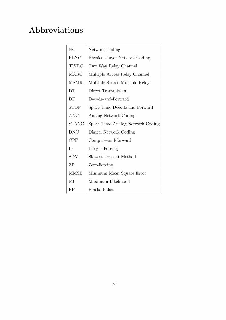
NC Network Coding

PLNC Physical-Layer Network Coding

TWRC Two Way Relay Channel

MARC Multiple Access Relay Channel

MSMR Multiple-Source Multiple-Relay

DT Direct Transmission

DF Decode-and-Forward

STDF Space-Time Decode-and-Forward

ANC Analog Network Coding

STANC Space-Time Analog Network Coding

DNC Digital Network Coding

CPF Compute-and-forward

IF Integer Forcing

SDM Slowest Descent Method

ZF Zero-Forcing

MMSE Minimum Mean Square Error

ML Maximum-Likelihood

FP Fincke-Pohst

v

List of Figures

2.1 MSMR model . . . . . . . . . . . . . . . . . . . . . . . . . . . . . . . . . 6

2.2 Time division allocation for one transmission realization . . . . . . . . . 6

2.3 Compute-and-Forward Diagram . . . . . . . . . . . . . . . . . . . . . . . 9

2.4 Candidate sets and rate tables for all relays . . . . . . . . . . . . . . . . 19

2.5 Constructing network coding system matrix A . . . . . . . . . . . . . . . 20

2.6 Probability of rank failure with local optimization for MSMR . . . . . . . 25

2.7 Rate comparisons with L = 3 for MSMR . . . . . . . . . . . . . . . . . . 26

2.8 Rate comparisons with L = 4 for MSMR . . . . . . . . . . . . . . . . . . 27

3.1 TWRC Model . . . . . . . . . . . . . . . . . . . . . . . . . . . . . . . . . 29

3.2 TWRC Diagram . . . . . . . . . . . . . . . . . . . . . . . . . . . . . . . 30

3.3 Probability of zero entry in TWRC . . . . . . . . . . . . . . . . . . . . . 37

3.4 Average rate comparisons for TWRC . . . . . . . . . . . . . . . . . . . . 38

4.1 MIMO diagram with independent data streams . . . . . . . . . . . . . . 41

4.2 IF decoder diagram . . . . . . . . . . . . . . . . . . . . . . . . . . . . . . 43

4.3 Creation of one slowest ascent line . . . . . . . . . . . . . . . . . . . . . . 46

4.4 The procedure of slowest descent method . . . . . . . . . . . . . . . . . . 47

4.5 IF performance regarding J (L=8,M=2) . . . . . . . . . . . . . . . . . . 53

4.6 Probability of successful IF matrix construction regarding J (L=8,M=2) 54

4.7 IF performance regarding M (L=8,J=4) . . . . . . . . . . . . . . . . . . 55

4.8 Rate comparisons of different linear detectors (L=4,J=2,M=2) . . . . . . 56



vi

5.1 System model A . . . . . . . . . . . . . . . . . . . . . . . . . . . . . . . . 61

5.2 Comparison of four schemes regarding system model A . . . . . . . . . . 66

5.3 System model B . . . . . . . . . . . . . . . . . . . . . . . . . . . . . . . . 67

5.4 Comparison of four schemes regarding system model B . . . . . . . . . . 73

5.5 System model C . . . . . . . . . . . . . . . . . . . . . . . . . . . . . . . . 74

5.6 Sum rate comparison for different schemes regarding system model C . . 82

5.7 BER comparison for different schemes regarding system model C . . . . . 83

5.8 System Model D . . . . . . . . . . . . . . . . . . . . . . . . . . . . . . . 84

5.9 The equivalent two separate MARC with two sources for DF . . . . . . . 88

5.10 The equivalent two separate MARC with two sources for DNC . . . . . . 90

5.11 Comparison of five schemes regarding system model D, σ2f = σ2

h = σ2g = 1 95

5.12 Comparison of five schemes regarding system model D: σ2f = 0.1, σ2

h =

σ2g = 1, . . . . . . . . . . . . . . . . . . . . . . . . . . . . . . . . . . . . . 96

5.13 Comparison of five schemes regarding system model D: σ2h = 0.1, σ2

f =

σ2g = 1 . . . . . . . . . . . . . . . . . . . . . . . . . . . . . . . . . . . . . 97

vii

List of Tables

3.1 Average number of candidate vectors for TWRC . . . . . . . . . . . . . . 39

5.1 Different Schemes for System Model A . . . . . . . . . . . . . . . . . . . 65

5.2 x1 ⊕ x2 for BPSK modulation . . . . . . . . . . . . . . . . . . . . . . . . 70

5.3 Different Schemes for System Model B . . . . . . . . . . . . . . . . . . . 72

5.4 Different Schemes for System Model C . . . . . . . . . . . . . . . . . . . 81

5.5 Different Schemes for System Model D . . . . . . . . . . . . . . . . . . . 94

viii

Abstract

The objective of this work is to investigate network coding design in wireless cooperative

networks. Along this line, our work can be divided into following subjects: (i) Compute-

and-forward strategy is one category of network coding in which a relay will decode and

forward a linear combination of source messages according to the observed channel co-

efficients, based on the algebraic structure of lattice codes. The destination will recover

all transmitted messages if enough linear equations are received. For multi-source multi-

relay wireless cooperative channels, we design in a system level, the compute-and-forward

network coding coefficients by Fincke-Pohst based candidate set searching algorithm and

network coding system matrix constructing algorithm, such that by those proposed al-

gorithms, the transmission rate of the multi-source multi-relay system is maximized.

Numerical results demonstrate the effectiveness of our proposed algorithms. (ii) We con-

sider the two-way relay channel (TWRC) of wireless cooperative system with compute-

and-forward network coding strategy. First a new lemma is proposed as network codes

search criteria for TWRC. Then, instead of exhaustive search, we present an efficient

network codes search algorithm based on modified Fincke-Pohst method. Numerical re-

sults demonstrate the effectiveness and complexity reduction of our proposed lemma and

algorithm. (iii) Based on the idea of compute-and-forward, integer forcing (IF) linear re-

ceiver architecture is for MIMO system to recover different integer combinations of lattice

codewords for further original message detection. In our work, we consider the problem of

IF linear receiver design with respect to the channel conditions. We present practical and

efficient algorithms to design the IF coefficient matrix with full rank such that the total

achievable rate is maximized, based on the slowest descent method. Numerical results

demonstrate the effectiveness of our proposed algorithms. (iv) We consider network cod-

ix

ing application in wireless multiple access relay channels with multiple-antenna relays.

We investigate several different relay techniques applicable for different system models,

including decode-and-forward (DF), space-time decode-and-forward (STDF), analog net-

work coding (ANC), space-time analog network coding (STANC), digital network coding

(DNC), etc. We describe in details those different schemes in different system models

with transmission time slots constraints, and compare the error rate performance.

x

Chapter 1

Introduction

1.1 Research Background

In the past decade, network coding [24] has rapidly emerged as a major research area

in electrical engineering and computer science. Originally designed for wired networks,

network coding is a generalized routing approach that breaks the traditional assumption

of simply forwarding data, and allows intermediate nodes to send out functions of their

received packets, by which the multicast capacity given by the max-flow min-cut theo-

rem can be achieved. Subsequent works of [25]-[27] made the important observation that,

for multicasting, intermediate nodes can simply send out a linear combination of their

received packets. Linear network coding with random coefficients is considered in [28].

In order to address the broadcast nature of wireless transmission, physical layer network

coding [29] was proposed to embrace interference in wireless networks in which interme-

diate nodes attempt to decode the modulo-two sum (XOR) of the transmitted messages.

Several network coding realizations in wireless networks are discussed in [31]-[30].

There is also a large body of works on lattice codes [36]-[37] and their applications

in communications. For many AWGN networks of interest, nested lattice codes [38]

can approach the performance of standard random coding arguments. It has been shown

that nested lattice codes (combined with lattice decoding) can achieve the capacity of the

point-to-point AWGN channel [39]. Subsequent work of [40] showed that nested lattice

codes achieve the diversity-multiplexing tradeoff of MIMO channel. In the two-way relay

1

networks, a nested lattice based strategy has been developed that the achievable rate is

near the optimal upper bound [45]-[47]. The nested lattice codes have the linear structure

that ensures that integer combinations of codewords are themselves codewords.

Compute-and-forward (CPF) strategy [48]-[49] is a promising new approach to physical-

layer network coding for general wireless networks, beneficial from both network coding

and lattice codes. The main idea is that a relay will decode a linear function of trans-

mitted messages according to the observed channel coefficients rather than ignoring the

interference as noise. Upon utilizing the algebraic structure of lattice codes, i.e., the

integer combination of lattice codewords is still a codeword, the intermediate relay n-

ode decodes and forwards an integer combination of original messages. With enough

linear independent equations, the destination can recover the original messages respec-

tively. Subsequent works for design and analysis of the CPF technique have been given

in [50]-[54].

As a research extension from the idea of CPF strategy, a new linear receiver technique

called integer forcing (IF) receiver for MIMO system has been proposed in [58]-[59]. In

MIMO communication, the destination often utilizes linear receiver architecture to reduce

implementation complexity with some performance sacrifice compared with maximum-

likelihood (ML) receiver. The standard linear detection methods include zero-forcing

(ZF) technique and the minimummean square error (MMSE) technique [56]. In the newly

proposed IF linear receiver, instead of attempting to recover a transmitted codeword

directly, each IF decoder recovers a different integer combination of the lattice codewords

according to a designed IF coefficient matrix. If the IF coefficient matrix is of full rank,

these linear equations can be solved for the original messages.

1.2 Research Contents of Each Chapter

In Chapter 2, we consider multi-source multi-relay channels with CPF network coding.

Previous works in CPF only consider the integer network coding coefficients optimization

of each relay locally/separately. However, for a multi-source multi-relay system with L

sources, separate optimizations cannot guarantee the network coding system matrix,

2

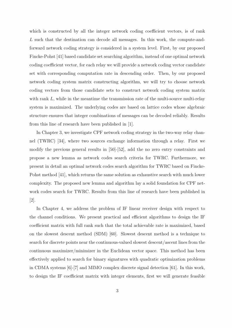
which is constructed by all the integer network coding coefficient vectors, is of rank

L such that the destination can decode all messages. In this work, the compute-and-

forward network coding strategy is considered in a system level. First, by our proposed

Fincke-Pohst [41] based candidate set searching algorithm, instead of one optimal network

coding coefficient vector, for each relay we will provide a network coding vector candidate

set with corresponding computation rate in descending order. Then, by our proposed

network coding system matrix constructing algorithm, we will try to choose network

coding vectors from those candidate sets to construct network coding system matrix

with rank L, while in the meantime the transmission rate of the multi-source multi-relay

system is maximized. The underlying codes are based on lattice codes whose algebraic

structure ensures that integer combinations of messages can be decoded reliably. Results

from this line of research have been published in [1].

In Chapter 3, we investigate CPF network coding strategy in the two-way relay chan-

nel (TWRC) [34], where two sources exchange information through a relay. First we

modify the previous general results in [50]-[52], add the no zero entry constraints and

propose a new lemma as network codes search criteria for TWRC. Furthermore, we

present in detail an optimal network codes search algorithm for TWRC based on Fincke-

Pohst method [41], which returns the same solution as exhaustive search with much lower

complexity. The proposed new lemma and algorithm lay a solid foundation for CPF net-

work codes search for TWRC. Results from this line of research have been published in

[2].

In Chapter 4, we address the problem of IF linear receiver design with respect to

the channel conditions. We present practical and efficient algorithms to design the IF

coefficient matrix with full rank such that the total achievable rate is maximized, based

on the slowest descent method (SDM) [60]. Slowest descent method is a technique to

search for discrete points near the continuous-valued slowest descent/ascent lines from the

continuous maximizer/minimizer in the Euclidean vector space. This method has been

effectively applied to search for binary signatures with quadratic optimization problems

in CDMA systems [6]-[7] and MIMO complex discrete signal detection [61]. In this work,

to design the IF coefficient matrix with integer elements, first we will generate feasible

3

searching set instead of the whole integer searching space based on the slowest descent

method. Then we try to pick up integer vectors within our searching set to construct

the full rank IF coefficient matrix, while in the meantime, the total achievable rate is

maximized. Results from this line of research have been published in [11] [16].

In Chapter 5, we carry out a study on network coding in multiple access relay channels

(MARC) with multiple antenna relay with different system model setting-ups. Under the

same transmission time slots constraint, we investigate several different relay techniques

applicable for different system models, including direct transmission (DT), decode-and-

forward (DF), space-time decode-and-forward (STDF), analog network coding (ANC),

space-time analog network coding (STANC), digital network coding (DNC), etc. We

describe in details those different schemes in different system models with transmission

time slots constraints, and compare the error rate performance. Results from this line of

research have been published in [13] [14] [17].

The notations used in this work are as follows. ·T denotes the transpose operation,

| · | represents the cardinality of a set, Zn denotes the n dimensional integer ring, Rn

denotes the n dimensional real field. Fp denotes a finite field of size p. In denotes the

identity matrix of size n×n, and 0 denotes the vectors with all zeros elements. Re(·) and

Im(·) denote the real part and the imaginary part. ∂f/∂(a) denotes the partial derivative

of function f regarding vector a. Assume that the log operation is with respect to base

2. We use boldface lowercase letters to denote column vectors and boldface uppercase

letters to denote matrices.

4

Chapter 2

Compute-and-Forward Network Coding

Design over Multi-Source Multi-Relay

Channels

2.1 Multi-Source Multi-Relay Channel

2.1.1 System Model

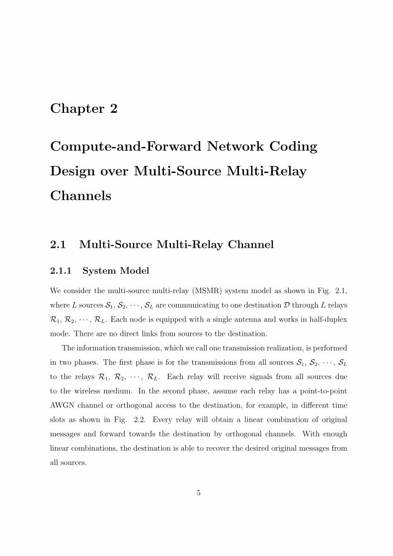
We consider the multi-source multi-relay (MSMR) system model as shown in Fig. 2.1,

where L sources S1, S2, · · · , SL are communicating to one destination D through L relays

R1, R2, · · · , RL. Each node is equipped with a single antenna and works in half-duplex

mode. There are no direct links from sources to the destination.

The information transmission, which we call one transmission realization, is performed

in two phases. The first phase is for the transmissions from all sources S1, S2, · · · , SL

to the relays R1, R2, · · · , RL. Each relay will receive signals from all sources due

to the wireless medium. In the second phase, assume each relay has a point-to-point

AWGN channel or orthogonal access to the destination, for example, in different time

slots as shown in Fig. 2.2. Every relay will obtain a linear combination of original

messages and forward towards the destination by orthogonal channels. With enough

linear combinations, the destination is able to recover the desired original messages from

all sources.

5

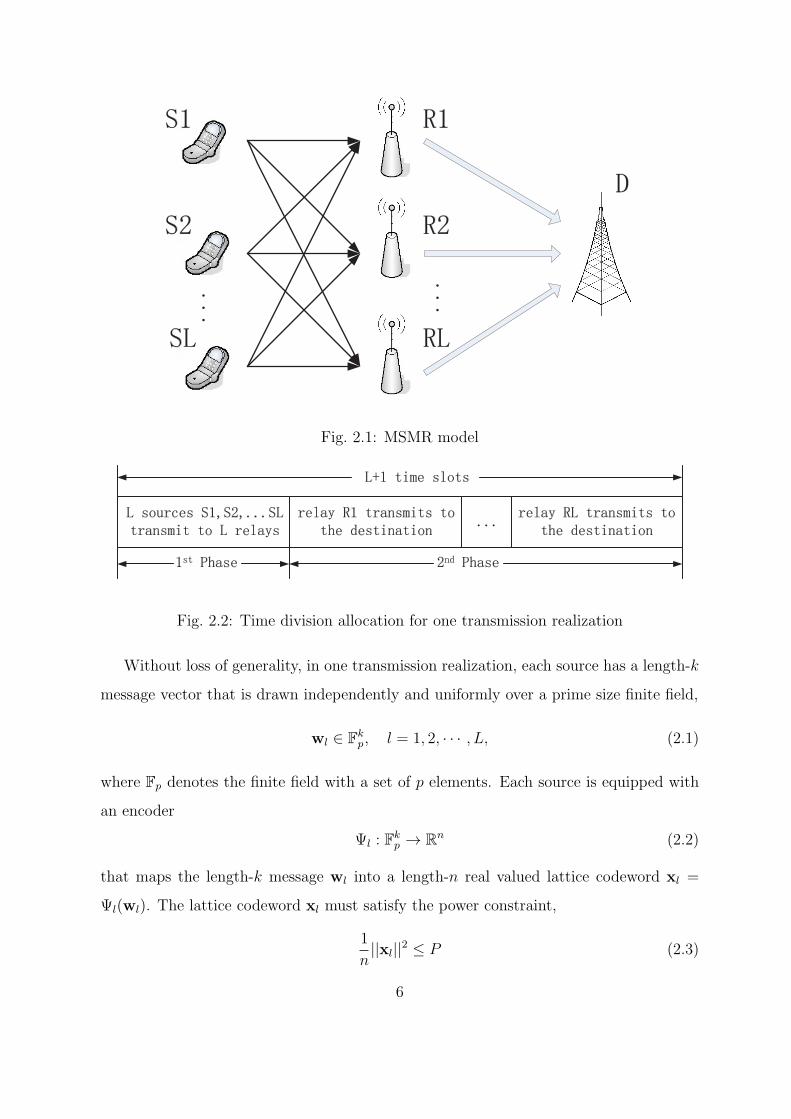
Fig. 2.1: MSMR model

Fig. 2.2: Time division allocation for one transmission realization

Without loss of generality, in one transmission realization, each source has a length-k

message vector that is drawn independently and uniformly over a prime size finite field,

wl ∈ Fkp, l = 1, 2, · · · , L, (2.1)

where Fp denotes the finite field with a set of p elements. Each source is equipped with

an encoder

Ψl : Fkp → Rn (2.2)

that maps the length-k message wl into a length-n real valued lattice codeword xl =

Ψl(wl). The lattice codeword xl must satisfy the power constraint,

1

n||xl||2 ≤ P (2.3)

6

for P ≥ 0 and l = 1, 2, · · · , L. The message rate, defined as the length of the message

measured in bits normalized by the number of channel uses R = knlog p [48], is the same

for all sources.

After mapping its message wl ∈ Fkp into a lattice codeword xl ∈ Rn, the source Sl

will send the codeword xl across the channel. Due to the broadcast nature of wireless

medium, the m-th relay will observe a noisy combination of the transmitted signals at

the end of the first phase,

ym =L∑l=1

hmlxl + zm, m = 1, 2, · · · , L, (2.4)

where hml ∈ R denotes real valued fading channel coefficient from Sl to relay Rm, gener-

ated i.i.d. according to a normal distribution N (0, 1); zm ∈ Rn denotes additive Gaussian

noise vector, zm ∼ N (0, In). Let

hm = [hm1, · · · , hmL]T (2.5)

denote the vector of channel coefficients from all sources to the m-th relay. We assume

this channel state information hm is available at relay m.

2.1.2 Compute-and-Forward Scheme

In a recent work, Nazer and Gastpar propose the compute-and-forward approach [48]

which exploits the property that any integer combination of lattice points is again a

lattice point. After receiving the noisy vector ym of (2.4), the m-th relay will first select

a scalar βm ∈ R and an integer network coding coefficient vector

am = [am1, am2, · · · , amL]T ∈ ZL, (2.6)

then attempt to decode the lattice point∑L

l=1 amlxl from

βmym =L∑l=1

βmhmlxl + βmzm (2.7)

=L∑l=1

amlxl +L∑l=1

(βmhml − aml)xl + βmzm︸︷︷︸Effective Noise

. (2.8)

7

Note that we do not need to conduct joint maximum likelihood (ML) decoding to get

(x1, x2, · · · , xL) for network coding. Instead we decode∑L

l=1 amlxl as one regular code-

word due to the lattice algebraic structure. In other words, the network coded codeword

is still in the same field as original source codeword.

In the finite field, it is equivalent that each relay is desired to reliably recover a linear

combination of the messages,

um =L⊕l=1

qmlwl =

[L∑l=1

amlwl

]mod p, (2.9)

where⊕

denotes summation over the finite field, qml is a coefficient taking values in Fp

and qml = aml mod p.

Each relay is equipped with a decoder,

Πm : Rn → Fkp, (2.10)

that maps the observed channel output ym ∈ Rn to an estimate

um = Πm(ym) ∈ Fkp (2.11)

of the message combination um. The diagram of compute-and-forward scheme is given

in Fig. 2.3.

We are interested in the rate of∑L

l=1 amlxl as a whole and will capture the perfor-

mance of the computation scheme by what we refer to as the computation rate, namely,

the number of bits of the linear function successfully recovered per channel use. The

work of [48] shows that a relay can often recover an equation of messages at a higher

rate than any individual message (or subset of message). The rate is highest when the

equation coefficients closely approximate the effective channel coefficients. The formal

statements are given in the following theorems [48]-[50]. Let log+(x)= max(log(x), 0).

Theorem 2.1.1 For real-valued AWGN networks with channel coefficient vector hm ∈

RL and desired network coding coefficient vector am ∈ ZL, the following computation rate

is achievable

Rm(am) = maxβm∈R

1

2log+

(P

β2m + P ||βmhm − am||2

). (2.12)

8

LY

2Y

1Y

M

1w

2w

Lw

1x

2x

Lx

1z

2z

Lz

1y

2y

Ly

1P

2P

LP

M

1u

2u

Lu

Fig. 2.3: Compute-and-Forward Diagram

Theorem 2.1.2 The computation rate given in Theorem 2.1.1 is uniquely maximized by

choosing βm to be the MMSE coefficient

βMMSE =P hT

mam

1 + P ||hm||2, (2.13)

which results in a computation rate of

Rm(am) =1

2log+

(||am||2 −

P (hTmam)

2

1 + P ||hm||2

)−1

. (2.14)

Theorem 2.1.3 For a given channel coefficient vector hm = [hm1, hm2, · · · , hmL]T ∈ RL,

Rm(am) is maximized by choosing the integer network coding coefficient vector am ∈ ZL

as

am = arg minam∈ZL,am =0

(aTmGmam

), (2.15)

where

Gm= I− P

1 + P ||hm||2Hm, (2.16)

and Hm = [H(m)ij ], H

(m)ij = hmihmj, 1 ≤ i, j ≤ L.

2.1.3 Problem Statement

Theorems 2.1.1-2.1.3 only give the optimal network coding integer coefficient vector am

and achievable computation rate Rm for each relay locally/separately and do not take

9

consideration of the overall system constraints. For the multi-source multi-relay system,

at the destination, enough linear combinations of the original messages need to be col-

lected. Let a1, a2, · · · , aL be the integer network coding coefficients vector for each relay,

then the network coding system matrix A at the destination can be denoted as

A = [a1, a2, · · · , aL]T . (2.17)

Hence, the destination can solve for the original packets if the network coding system

matrix A has full rank L, i.e. |A| = 0. In which case, as the same rate of source-relay

channels in phase I is available for relay-destination channels in phase II, the transmission

rate at the destination is dominated/bottlenecked by

RD = min R1,R2, · · · ,RL . (2.18)

We can easily understand that after calculating the integer network coding coefficient

vector am for each relay by theorems 2.1.1-2.1.3 to maximize its own computation rate,

the network coding system matrix A constructed by those integer vectors may not have

full rank L, in which case the destination cannot decode the original messages by those

linear equations. In other words, we cannot fix the optimal integer network coding vector

am for each relay separately, since it cannot guarantee that the system constraint of full

rank A.

Therefore, we need to optimize the integer network coding vectors for L relays in

a overall system level. Instead of distributed calculations, to construct the full rank

network coding system matrix that maximize the overall message rate at destination, A

will be designed according to the following criteria

A = arg max|A|=0

RD

= arg max|A|=0

(min R1,R2, · · · ,RL)

= arg max|A|=0

minm=1,···L

(1

2log+

(||am||2 −

P (hTmam)

2

1 + P ||hm||2

)−1).

(2.19)

In other words, we need to find the integer network coding vectors a1, a2, · · · , aL, under

10

the system level constraint of full rank A, to maximize the computation rate of each relay

R1, R2, · · · , RL jointly, such that the minimum value of R1, R2, · · · , RL is maximized.

Equivalently, the optimum network coding system matrix A should be

A = arg min|A|=0

maxm=1,···L

aTmGmam, (2.20)

where Gm is defined in (2.16).

2.2 Proposed Strategy

In this work, to approach the overall system optimization of (2.19)-(2.20), we propose

the following novel strategy which includes two steps. In the first step, for relay m,

instead of finding one optimal network coding coefficient vector am to maximize its own

computation rate, we are trying to find a candidate set

ΩTmaxm = a(1)

m , a(2)m , · · · , a(Tmax)

m , (2.21)

with |ΩTmaxm | = Tmax. The network coding coefficient vectors with the top Tmax maximum

computation rates for relay m are within the candidate set ΩTmaxm . Note that Tmax is

a parameter to control the candidate set length for each relay and currently set by

experience/simulation. We will propose an algorithm based on Fincke-Pohst Method

[41] to find the network coding coefficient vector candidate set for each relay.

After we get all the candidate vector sets ΩTmax1 , ΩTmax

2 , · · · , ΩTmaxL , in the second step,

we will try to pick up a1 ∈ ΩTmax1 , a2 ∈ ΩTmax

2 , · · · , aL ∈ ΩTmaxL , to construct the full

rank network coding coefficient matrix A = [a1, a2, · · · , aL]T , while in the meantime, the

minimum value of corresponding R1(a1), R2(a2), · · · , RL(aL) is maximized.

2.2.1 Searching Candidate Set ΩTmaxm for Each Relay

For relay m, we are trying to find the candidate set ΩTmaxm = a(1)

m , a(2)m , · · · , a(Tmax)

m

with |ΩTmaxm | = Tmax, such that the network coding coefficient vectors with the top Tmax

maximum computation rate for relay m are within. According to Theorem 2.1.3, it is

11

equivalent to find the set ΩTmaxm with Tmax vectors, such that those vectors give the bottom

Tmax minimum aTmGmam values, where Gm is defined in (2.16).

The searching of candidate set Ωmaxm with fixed length Tmax can be decomposed into

following steps.

(1) Enumerate all vectors t ∈ ZL (t = 0) in Ωm, such that tTGmt ≤ C for a given

positive constant C, i.e.,

Ωm =t : tTGmt ≤ C, t = 0, t ∈ ZL

. (2.22)

(2) Adjust the constant C to guarantee that |Ωm| ≥ Tmax.

(3) Sort all the vectors t1, t2, · · · , t|Ωm| in Ωm in descending order corresponding to

the computation rate value Rm in (2.14), such that

Rm(t1) ≥ Rm(t2) ≥ · · · ≥ Rm(t|Ωm|). (2.23)

(4) Pick the first Tmax vectors of Ωm to form the set ΩTmaxm .

The procedure of enumerating all vectors t ∈ ZL (t = 0) in Ωm, such that tTGmt ≤ C

for a given positive constant C is based on the Fincke-Pohst Method and derived as

follows.

We operate Cholesky’s factorization of matrix Gm,

Gm = UTU, (2.24)

where U is an upper triangular matrix. Denote || · ||F for the Frobenius norm. Let uij,

i, j = 1, 2, · · · , L, be the entries of the upper triangular matrix U and

t = [t1, t2, · · · , tL]T . (2.25)

12

Then, the searching vector t that makes tTGmt ≤ C can be expressed as

tTGmt = ||U t||2F =L∑i=1

(uiiti +

L∑j=i+1

uijtj

)2

=L∑i=1

gii

(ti +

L∑j=i+1

gijtj

)2

=L∑

i=k

gii

(ti +

L∑j=i+1

gijtj

)2

+k−1∑i=1

gii

(ti +

L∑j=i+1

gijtj

)2

≤ C (2.26)

where gii = u2ii and gij = uij/uii for i = 1, 2, · · · , L, j = i + 1, · · · , L. Obviously the

second term of (2.26) is non-negative, hence, to satisfy (2.26), it is equivalent to consider

for every k = L,L− 1, · · · , 1,

L∑i=k

gii

(ti +

L∑j=i+1

gijtj

)2

≤ C. (2.27)

Then, we can start work backwards to find the bounds for vector entries tL, tL−1, · · · , t1one by one.

We begin to evaluate the last element tL of the searching vector t. Referring to (2.27)

and let k = L, we have

gLLt2L ≤ C. (2.28)

Set ∆L = 0, CL = C, and we will get

LBL ≤ tL ≤ UBL, (2.29)

with

UBL =

⌊ √CL

gLL−∆L

⌋, LBL =

⌈−

√CL

gLL−∆L

⌉, (2.30)

where ⌈x⌉ is the smallest integer no less than x and ⌊x⌋ is the greatest integer no bigger

than x.

Next, we evaluate the element tL−1 of the searching vector t. Referring to (2.27) and

let k = L− 1, we have

gLLt2L + gL−1,L−1 (tL−1 + gL−1,LtL)

2 ≤ C, (2.31)

13

which leads to⌈−

√C − gLLt2LgL−1,L−1

− gL−1,LtL

⌉≤ tL−1 ≤

⌊ √C − gLLt2LgL−1,L−1

− gL−1,LtL

⌋. (2.32)

If we denote ∆L−1 = gL−1,LtL, CL−1 = C − gLLt2L, the bounds for sL−1 can be expressed

as

LBL−1 ≤ tL−1 ≤ UBL−1, (2.33)

where

UBL−1 =

⌊√CL−1

gL−1,L−1

−∆L−1

⌋, LBL−1 =

⌈−

√CL−1

gL−1,L−1

−∆L−1

⌉. (2.34)

We can see that given radius√C and matrix U, the bounds for tL−1 only depends on

the previous evaluated tL, and not correlated with tL−2, tL−3, · · · , t1.

In a similar fashion, we can proceed for tL−2 evaluation, and so on.

To evaluate the element tk of the searching vector t, referring to (2.27) we will have

L∑i=k

gii

(ti +

L∑j=i+1

gijtj

)2

≤ C, (2.35)


√1

gkk

(C −

∑Li=k+1 gii

(ti +

∑Lj=i+1 gijtj

)2)−∑L

j=k+1 gkjtj

⌉

≤ tk ≤

⌊ √1

gkk

(C −

∑Li=k+1 gii

(ti +

∑Lj=i+1 gijtj

)2)−∑L

j=k+1 gkjtj

⌋.

If we denote

∆k =L∑

j=k+1

gkjtj,

Ck = C −L∑

i=k+1

gii

(ti +

L∑j=i+1

gijtj

)2

, (2.36)

the bounds for sk can be expressed as

LBk ≤ tk ≤ UBk, (2.37)

14

where

UBk =

⌊ √Ck

gkk−∆k

⌋, LBk =

⌈−

√Ck

gkk−∆k

⌉. (2.38)

Note that for given radius√C and matrix U, the bounds for tk only depends on the

previous evaluated tk+1, tk+2, · · · , tL.

Finally, we evaluate the element t1 of the searching vector t. Referring to (2.27) and

let k = 1, we will haveL∑i=1

gii

(ti +

L∑j=i+1

gijtj

)2

≤ C, (2.39)


√1g11

(C −

∑Li=2 gii

(ti +

∑Lj=i+1 gijtj

)2)−∑L

j=2 g1jtj

⌉

≤ t1 ≤

⌊ √1g11

(C −

∑Li=2 gii

(ti +

∑Lj=i+1 gijtj

)2)−∑L

j=2 g1jtj

⌋. (2.40)

If we denote

∆1 =L∑

j=2

g1jtj,

C1 = C −L∑i=2

gii

(ti +

L∑j=i+1

gijtj

)2

, (2.41)

the bounds for t1 can be expressed as

LB1 ≤ t1 ≤ UB1, (2.42)

where

UB1 =

⌊ √C1

g11−∆1

⌋, LB1 =

⌈−

√C1

g11−∆1

⌉. (2.43)

In practice, CL, CL−1, · · · , C1 can be updated recursively by the following equations

∆k =L∑

j=k+1

gkjtj, (2.44)

Ck = C −L∑

i=k+1

gii

(ti +

L∑j=i+1

gijtj

)2

= Ck+1 − gk+1,k+1 (∆k+1 + tk+1)2 , (2.45)

15

for k = L− 1, L− 2, · · · , 1 and ∆L = 0, CL = C.

The entries tL, tL−1, · · · , t1 are chosen as follows: for a chosen candidate of tL satisfying

the bounds (2.29)-(2.30), we can choose a candidate for tL−1 satisfying the bounds (2.33)-

(2.34). If a candidate value for tL−1 does not exist, we go back to (2.29)-(2.30) and choose

other candidate value tL. Then search for tL−1 that meets the bounds (2.33)-(2.34) for the

given tL. If tL and tL−1 are chosen as candidates, we follow the same procedure to choose

tL−2, and so on. When a set of tL, tL−1, · · · , t1 is chosen and satisfies all corresponding

bounds requirements, one candidate vector t = [t1, t2, · · · , tL]T is obtained. We record

all the candidate vectors satisfying their bounds requirements, such that all vectors meet

tTGmt ≤ C will be in Ωm.

Regarding the setting of positive constant C, we will set it based on the binary vector

obtained by applying the direct sign operator of the real minimum-eigenvalue eigenvector

of Gm, denoted as tquant, such that

C = tTquantGm tquant. (2.46)

By setting the searching sphere radius this way, it is big enough to have at least one

searching vector tquant falls inside, while in the meantime small enough to have not too

many searching vectors within.

Note that this searching procedure will return all candidates that satisfy tTGmt ≤

C. There is at least one candidate vector tquant such that its entries satisfy all the

bounds requirements. On the other hand, the maximum likelihood (ML) exhaustive

search among all t ∈ ZL, with optimal result tML that returns the minimum metric

tTGmt, or equivalently maximum the computation rate for one relay, will also fall inside

the search bounds, since

tTMLGmtML ≤ tTquantGm tquant = C. (2.47)

Hence, we are guaranteed to include the local optimal network coding coefficient vector,

which maximizes the computation rate for one relay m, in ΩTmaxm .

We summarize our proposed algorithm for the searching candidate set ΩTmaxm for relay

m based on Fincke-Pohst method as follows.

16

Algorithm 2.1 FP Based Candidate Set Searching Algorithm

Input: Matrix Gm, Tmax = |ΩTmaxm |.

Output: The candidate vector set ΩTmaxm and corresponding computation rate set ΓTmax

m .

Step 1: Calculate the binary quantized vector obtained by applying the direct sign op-

erator of the real minimum-eigenvalue eigenvector of Gm, denoted as tquant, and set C

as

C = tTquantGm tquant. (2.48)

Step 2: Operate Cholesky’s factorization of matrix Gm, Gm = UTU, where U is an

upper triangular matrix. Let uij, i, j = 1, 2, · · · , L denote the entries of matrix U. Set

gii = u2ii, gij = uij/uii,

for i = 1, 2, · · · , L, j = i+ 1, · · · , L.

Step 3: Search set Ωm =t : tTGmt ≤ C, t = 0, t ∈ ZL

according to the following

Fincke-Pohst procedure.

(i) Start from ∆L = 0, CL = C, k = L and Ωm = ∅.

(ii) Set the upper bound UBk and the lower bound LBk as follows

UBk =

⌊ √Ck

gkk−∆k

⌋, LBk =

⌈−

√Ck

gkk−∆k

⌉,

and tk = LBk − 1.

(iii) Set tk = tk + 1. For tk ≤ UBk, go to (v); else go to (iv).

(iv) If k = L, terminate and output Ωm; else set k = k + 1 and go to (iii).

(v) For k = 1, go to (vi); else set k = k − 1, and

∆k =L∑

j=k+1

gkjtj,

Ck = Ck+1 − gk+1,k+1 (∆k+1 + tk+1)2 ,

then go to (ii).

17

(vi) If t = 0 terminate, else we get a candidate vector t = 0 that satisfies all the bounds

requirements and put it inside Ωm, i.e. Ωm = Ωm, t. Go to (iii).

Step 4: If |Ωm| < Tmax, set C = 2C and repeat Step 3.

Step 5: Sort all the vectors t1, t2, · · · , t|Ωm| in Ωm in descending order corresponding to

the computation rate value Rm in (2.14), such that

Rm(t1) ≥ Rm(t2) ≥ · · · ≥ Rm(t|Ωm|). (2.49)

Pick the first Tmax vectors of Ωm to form the set ΩTmaxm and construct the corresponding

computation rate ΓTmaxm as ΩTmax

m = t1, t2, · · · , tTmax,

ΓTmaxm = Rm(t1),Rm(t2), · · · ,Rm(tTmax).

(2.50)

2.2.2 Constructing Network Coding Matrix A

According to our proposed FP Based Candidate Set ΩTmaxm Searching Algorithm 1, for

relay m, we get the candidate set ΩTmaxm for integer network coding coefficient vector

am. The set ΩTmaxm consists Tmax candidates vectors ΩTmax

m = a(1)m , a

(2)m , · · · , a(Tmax)

m , in

which a(1)m , a

(2)m , · · · , a(Tmax)

m have been sorted such that Rm(a(1)m ) ≥ Rm(a

(2)m ) ≥ · · · ≥

Rm(a(Tmax)m ). Denote R(i)

m = Rm(a(i)m ), i = 1, 2, · · · , Tmax. Then for each relay we can

have two length-Tmax tables as shown in Fig. 2.4,

Table 1: ΓTmaxm = R(1)

m ,R(2)m , · · · ,R(Tmax)

m , (2.51)

Table 2: ΩTmaxm = a(1)

m , a(2)m , · · · , a(Tmax)

m . (2.52)

The second table consists the sorted candidate vector set ΩTmaxm , while the first one

consists the corresponding computation rate set ΓTmaxm with elements R(1)

m ≥ R(2)m ≥

· · · ≥ R(Tmax)m .

After we get all the candidate vector sets ΩTmax1 , ΩTmax

2 , · · · , ΩTmaxL and computation

rate sets ΓTmax1 , ΓTmax

2 , · · · , ΓTmaxL , we will try to pick up a1 ∈ ΩTmax

1 , a2 ∈ ΩTmax2 , · · · ,

18

)(

1

)2(

1

)1(

1maxT

aaa L

maxT

1W

maxT

1G

)(

1

)2(

1

)1(

1maxT

RRR L

)(

2

)2(

2

)1(

2maxT

aaa L

maxT

2W

maxT

2G

)(

2

)2(

2

)1(

2maxT

RRR L

)()2()1( maxT

LLLaaa L

maxT

LW

maxT

LG

)()2()1( maxT

LLLRRR L

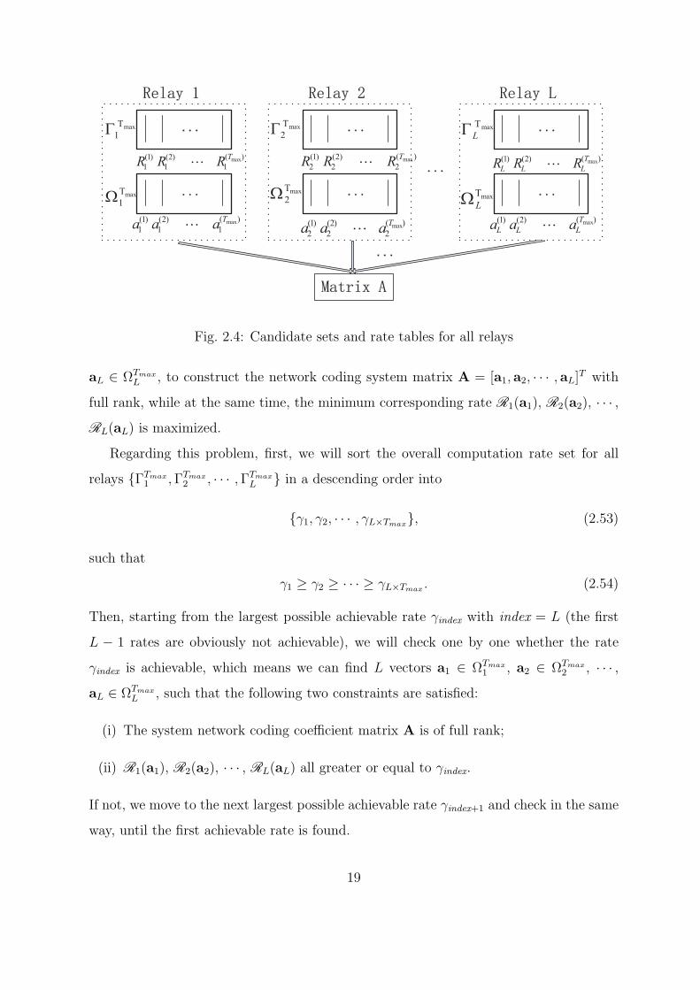
Fig. 2.4: Candidate sets and rate tables for all relays

aL ∈ ΩTmaxL , to construct the network coding system matrix A = [a1, a2, · · · , aL]

T with

full rank, while at the same time, the minimum corresponding rate R1(a1), R2(a2), · · · ,

RL(aL) is maximized.

Regarding this problem, first, we will sort the overall computation rate set for all

relays ΓTmax1 ,ΓTmax

2 , · · · ,ΓTmaxL in a descending order into

γ1, γ2, · · · , γL×Tmax, (2.53)

such that

γ1 ≥ γ2 ≥ · · · ≥ γL×Tmax . (2.54)

Then, starting from the largest possible achievable rate γindex with index = L (the first

L − 1 rates are obviously not achievable), we will check one by one whether the rate

γindex is achievable, which means we can find L vectors a1 ∈ ΩTmax1 , a2 ∈ ΩTmax

2 , · · · ,

aL ∈ ΩTmaxL , such that the following two constraints are satisfied:

(i) The system network coding coefficient matrix A is of full rank;

(ii) R1(a1), R2(a2), · · · , RL(aL) all greater or equal to γindex.

If not, we move to the next largest possible achievable rate γindex+1 and check in the same

way, until the first achievable rate is found.

19

index

Tcut

R g³)(

11

cut

1W

)(

1

)(

1

)1(

1max1 TT

aaacut

LL

maxT

1W

maxT

1G

)(

1

)(

1

)1(

1max1 TT

RRRcut

LL

cut

mW

)()()1( maxT

m

n

mmaaa LL

maxT

mW

maxT

mG

)()()1( maxT

m

n

mmRRR LL

index

n

mR g=)(

index

T

L

cut

LR g³)(

cut

LW

)()()1( maxT

L

T

LLaaa

cut

L LL

maxT

LW

maxT

LG

)()()1( maxT

L

T

LLRRR

cut

L LL

Fig. 2.5: Constructing network coding system matrix A

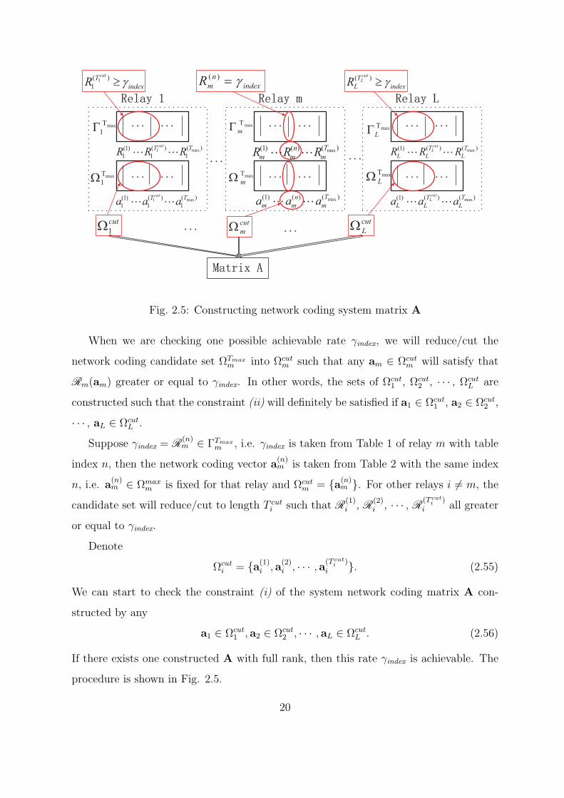
When we are checking one possible achievable rate γindex, we will reduce/cut the

network coding candidate set ΩTmaxm into Ωcut

m such that any am ∈ Ωcutm will satisfy that

Rm(am) greater or equal to γindex. In other words, the sets of Ωcut1 , Ωcut

2 , · · · , ΩcutL are

constructed such that the constraint (ii) will definitely be satisfied if a1 ∈ Ωcut1 , a2 ∈ Ωcut

2 ,

· · · , aL ∈ ΩcutL .

Suppose γindex = R(n)m ∈ ΓTmax

m , i.e. γindex is taken from Table 1 of relay m with table

index n, then the network coding vector a(n)m is taken from Table 2 with the same index

n, i.e. a(n)m ∈ Ωmax

m is fixed for that relay and Ωcutm = a(n)

m . For other relays i = m, the

candidate set will reduce/cut to length T cuti such that R(1)

i , R(2)i , · · · , R

(T cuti )

i all greater

or equal to γindex.

Denote

Ωcuti = a(1)

i , a(2)i , · · · , a(T cut

i )i . (2.55)

We can start to check the constraint (i) of the system network coding matrix A con-

structed by any

a1 ∈ Ωcut1 , a2 ∈ Ωcut

2 , · · · , aL ∈ ΩcutL . (2.56)

If there exists one constructed A with full rank, then this rate γindex is achievable. The

procedure is shown in Fig. 2.5.

20

We summarize this procedure to constructing the full rank network coding system

matrix A with candidate sets ΩTmax1 , ΩTmax

2 , · · · , ΩTmaxL and the corresponding computa-

tion rate sets ΓTmax1 , ΓTmax

2 , · · · , ΓTmaxL as follows.

Algorithm 2.2 Network Coding System Matrix Constructing Algorithm

Input: Candidate vector sets ΩTmax1 , ΩTmax

2 , · · · , ΩTmaxL ;

Computation rate sets ΓTmax1 , ΓTmax

2 , · · · , ΓTmaxL .

Output: The network coding system matrix A constructed from a1 ∈ ΩTmax1 , a2 ∈ ΩTmax

2 ,

· · · , aL ∈ ΩTmaxL with full rank that gives the maximum transmission rate Rmax

D .

Step 1: Sort the overall computation rate set for all relays ΓTmax1 ,ΓTmax

2 , · · · ,ΓTmaxL in a

descending order into γ1, γ2, · · · , γL×Tmax, such that γ1 ≥ γ2 ≥ · · · ≥ γL×Tmax . Initialize

index = L.

Step 2: Check whether the rate of γindex is achievable by the following procedure. Suppose

γindex = R(n)m ∈ ΓTmax

m . Then, for relay i, the reduced candidate set Ωcuti , i = 1, 2, · · · , L

will be constructed as follows.

(i) For relay m, set Ωcutm = a(n)

m .

(ii) For relay i = m, compare the value of γindex and the sorted descending set ΓTmaxi =

R(1)i , R(2)

i , · · · , R(Tmax)i . Find all R(1)

i , R(2)i , · · · , R

(T cuti )

i greater or equal to

γindex. Set Ωcuti = a(1)

i , a(2)i , · · · , a(T cut

i )i .

Step 3: Check every a1 ∈ Ωcut1 , a2 ∈ Ωcut

2 , · · · , aL ∈ ΩcutL , until we find one network

coding system matrix A = [a1, a2, · · · , aL]T has full rank, i.e. |A| = 0. If so, terminate

and output the network coding system matrix A and the maximum transmission rate

RmaxD = γindex.

Step 4: If for any a1 ∈ Ωcut1 , a2 ∈ Ωcut

2 , · · · , aL ∈ ΩcutL , we cannot construct a full rank

network coding system matrix A, then set index = index+ 1, go to Step 2.

One possible implementation of the whole system will let relays calculate the candi-

21

date sets and corresponding computation rate sets, construct the optimal network coding

system matrix A, then transmit the L×L integers matrix A to the destination. Another

possible implementation is to allow the destination work as processing center, that does

all calculations, including candidate sets, corresponding computation rate sets, and the

optimal network coding system matrix A construction. The destination will then feed-

back the optimal network coding vector am ∈ ZL to relay m for m = 1, 2, · · · , L. After

system initialization, these optimal network coding vectors can be used for the system

when the channels are stationary.

2.3 Experimental Studies

2.3.1 A Transparent Realization

In this subsection, we will give a detailed experimental example to show our proposed

algorithms in a transparent way. For a three-source three-relay system with L = 3, we

set the power constraints P = 10dB and Tmax = 5. The channel coefficient vector hm for

each relay is generated as

h1 = [0.9730, 0.4674, 0.5103]T ,

h2 = [−1.7291, 0.7166,−0.5856]T ,

h3 = [−0.3912, 1.4407,−0.8115]T .

After calculating Gm, m = 1, 2, 3 and running our proposed FP based candidate

set searching algorithm for each relay, we will get the network coding candidate vector

sets ΩTmax1 , ΩTmax

2 , ΩTmax3 and corresponding computation rate sets ΓTmax

1 , ΓTmax2 , ΓTmax

3 as

follows

ΩTmax1 =

1 2 1 1 1

0 1 1 0 1

0 1 1 1 0

,

ΓTmax1 = [0.4846, 0.4620, 0.3408, 0.2918, 0.2231] ;

22

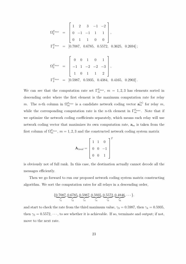
ΩTmax2 =

1 2 3 −1 −2

0 −1 −1 1 1

0 1 1 0 0

,

ΓTmax2 = [0.7087, 0.6785, 0.5572, 0.3625, 0.2694] ;

ΩTmax3 =

0 0 1 0 1

−1 1 −2 −2 −3

1 0 1 1 2

,

ΓTmax3 = [0.5987, 0.5935, 0.4384, 0.4165, 0.2902] .

We can see that the computation rate set ΓTmaxm , m = 1, 2, 3 has elements sorted in

descending order where the first element is the maximum computation rate for relay

m. The n-th column in ΩTmaxm is a candidate network coding vector a

(n)m for relay m,

while the corresponding computation rate is the n-th element in ΓTmaxm . Note that if

we optimize the network coding coefficients separately, which means each relay will use

network coding vector that maximizes its own computation rate, am is taken from the

first column of ΩTmaxm , m = 1, 2, 3 and the constructed network coding system matrix

Alocal =

1 1 0

0 0 −1

0 0 1

T

is obviously not of full rank. In this case, the destination actually cannot decode all the

messages efficiently.

Then we go forward to run our proposed network coding system matrix constructing

algorithm. We sort the computation rates for all relays in a descending order,

0.7087︸︷︷︸γ1

, 0.6785︸︷︷︸γ2

, 0.5987︸︷︷︸γ3

, 0.5935︸︷︷︸γ4

, 0.5572︸︷︷︸γ5

, 0.4846︸︷︷︸γ6

, · · · .

and start to check the rate from the third maximum value, γ3 = 0.5987, then γ4 = 0.5935,

then γ5 = 0.5572, · · · , to see whether it is achievable. If so, terminate and output; if not,

move to the next rate.

23

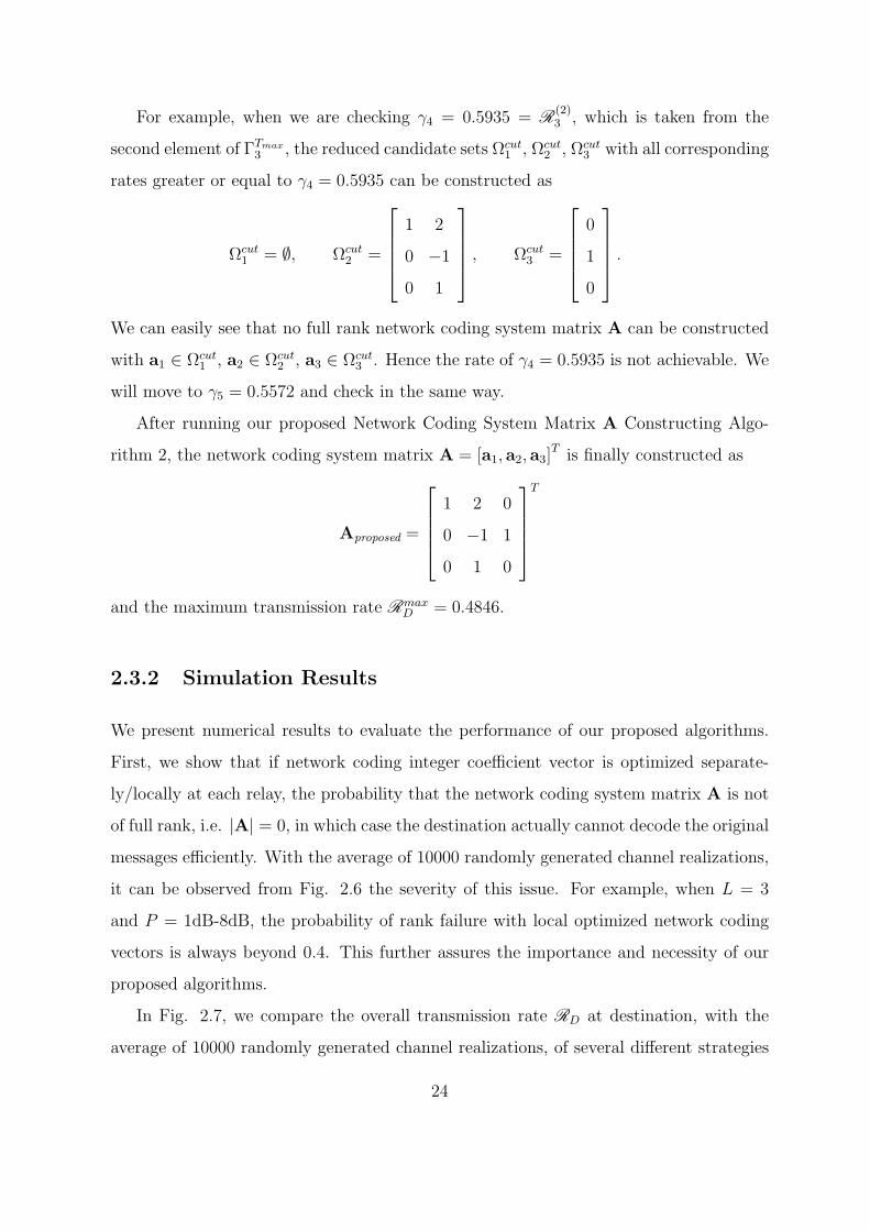
For example, when we are checking γ4 = 0.5935 = R(2)3 , which is taken from the

second element of ΓTmax3 , the reduced candidate sets Ωcut

1 , Ωcut2 , Ωcut

3 with all corresponding

rates greater or equal to γ4 = 0.5935 can be constructed as

Ωcut1 = ∅, Ωcut

2 =

1 2

0 −1

0 1

, Ωcut3 =

0

1

0

.

We can easily see that no full rank network coding system matrix A can be constructed

with a1 ∈ Ωcut1 , a2 ∈ Ωcut

2 , a3 ∈ Ωcut3 . Hence the rate of γ4 = 0.5935 is not achievable. We

will move to γ5 = 0.5572 and check in the same way.

After running our proposed Network Coding System Matrix A Constructing Algo-

rithm 2, the network coding system matrix A = [a1, a2, a3]T is finally constructed as

Aproposed =

1 2 0

0 −1 1

0 1 0

T

and the maximum transmission rate RmaxD = 0.4846.

2.3.2 Simulation Results

We present numerical results to evaluate the performance of our proposed algorithms.

First, we show that if network coding integer coefficient vector is optimized separate-

ly/locally at each relay, the probability that the network coding system matrix A is not

of full rank, i.e. |A| = 0, in which case the destination actually cannot decode the original

messages efficiently. With the average of 10000 randomly generated channel realizations,

it can be observed from Fig. 2.6 the severity of this issue. For example, when L = 3

and P = 1dB-8dB, the probability of rank failure with local optimized network coding

vectors is always beyond 0.4. This further assures the importance and necessity of our

proposed algorithms.

In Fig. 2.7, we compare the overall transmission rate RD at destination, with the

average of 10000 randomly generated channel realizations, of several different strategies

24

2 4 6 8 10 12 140.1

0.2

0.3

0.4

0.5

0.6

0.7

0.8

Power constraint P in dB

Pro

babi

lity

of r

ank

failu

re w

ith lo

cal o

ptim

izat

ion

L=2L=3L=4

Fig. 2.6: Probability of rank failure with local optimization for MSMR

in multi-source multi-relay channels with L = 3 and Tmax = 5. (i) The “DF with

interference as noise” is a strategy in which relay m is trying to decode one message

from source m and treat other messages as noise. In this special case, the system matrix

A = IL. (ii) The “CPF NC with Round-H” is a strategy that each relay decodes a linear

integer combination of transmitted messages, while the network coding coefficients are

set by a simplified method, i.e. rounding the channel coefficients directly to the nearest

integers. (iii) The “CPF NC with local optimization” is a strategy that each relay also

decodes a linear integer combination of transmitted messages, while the network coding

coefficients are optimized locally/separately. Due to the rank failure issue of network

coding system matrix, in which case the destination cannot decode all messages, the

rate is decreased. Finally, (iv) the “CPF NC with proposed algorithms” is the strategy

25

that each relay decodes a linear integer combination of transmitted messages with our

proposed FP based candidate set searching algorithm and network coding system matrix

constructing algorithm.

2 4 6 8 10 12 140

0.1

0.2

0.3

0.4

0.5

0.6

0.7

0.8


Ave

rage

rat

e of

diff

eren

t sch

emes

DF with interference as noise

CPF NC with Round−H

CPF NC with local optimization

CPF NC with proposed algorithms

Fig. 2.7: Rate comparisons with L = 3 for MSMR

As shown in Fig. 2.7, the performance differences are significant. “DF with interfer-

ence as noise” gives very poor result. Furthermore, increasing power constraint has not

much effect on this strategy since as the power increases for the interested message, the

corresponding interference power is also raised. The “CPF NC with Round-H” strategy

works a little better since it somehow takes advantage of network coding to improve the

rate, but the coefficients are chosen in a simplified way and not optimal. The “CPF

NC with proposed algorithms” strategy, in which case the network coding coefficients are

optimized systematically, performs superior to all other strategies and has about 3dB

26

gain compared with the “CPF NC with local optimization”.

2 4 6 8 10 12 140

0.1

0.2

0.3

0.4

0.5

0.6

0.7


Ave

rage

rat

e of

diff

eren

t sch

emes

DF with interference as noise

CPF NC with Round−H

CPF NC with local optimization

CPF NC with proposed algorithms

Fig. 2.8: Rate comparisons with L = 4 for MSMR

We repeat our experiment with multi-source multi-relay channels of L = 4 and present

the average rate comparisons of different schemes with respect to the power constraint.

Similar results are shown as in Fig. 2.8. “CPF NC with proposed algorithms” strategy still

gives the best performance and further demonstrates the effectiveness of our proposed

algorithms.

27

2.4 Conclusion

In this work, we consider the problem of integer network coding coefficients design in

a system level over a compute-and-forward multi-source multi-relay system. Instead of

optimizing network coding vector of each relay separately, we propose the Fincke-Pohst

based candidate set searching algorithm, to provide a network coding vector candidate

set for each relay with corresponding computation rate in descending order. Then, with

our proposed network coding system matrix constructing algorithm, we choose network

coding vectors from candidate sets to construct network coding system matrix with full

rank, while in the meantime the transmission rate of the overall system is maximized. Nu-

merical results give the performance comparisons of our proposed compute-and-forward

network coding algorithms and other strategies.

28

Chapter 3

Efficient Compute-and-Forward Network

Codes Search for Two-Way Relay Channel

3.1 System Model

Consider the classic TWRC with two sources S1, S2 attempting to exchange information

with each other through a relay R as in Fig. 3.1. There is no direct link between two

sources and each node is equipped with one antenna.

Fig. 3.1: TWRC Model

Without loss of generality, in one information codeword transmission, each source has

a length-k information vector

wm ∈ Fkp, (3.1)

m = 1, 2, where Fp = 0, 1, · · · , p−1 is a prime size finite field. Each source is equipped

with an encoder

Em : Fkp → Rn (3.2)

29

that maps the length-k message wm into a length-n lattice codeword

xm ∈ Rn. (3.3)

The codeword satisfies the power constraint of

1

n||xm||2 ≤ P. (3.4)

The information transmission includes two phases. In the first phase, two sources

S1, S2 transmit simultaneously to relay R, which can be modeled by a multiple-access

channel with inputs x1, x2 and output yR. In the second phase, relay R broadcast to S1

and S2, which can be modeled by a broadcast channel with input xR and outputs y1 and

y2. The transmission diagram of TWRC is shown in Fig. 3.2.

1w 2

w1x 2

x

Ry

Rx

1y

2y

Fig. 3.2: TWRC Diagram

At the end of first phase, relay R will receive

yR = h1x1 + h2x2 + zR, (3.5)

where h1, h2 ∈ R are real valued fading channel coefficient from S1 and S1 to relay

R respectively and zR ∈ Rn is additive Gaussian noise. All channel coefficients are

generated i.i.d. according to a normal distribution N (0, 1).

30

In the framework of CPF [50], the property that any integer combination of lattice

codewords is again a lattice codeword is exploited. After receiving the noisy vector yR,

relayR will select a scalar β ∈ R and an integer network coding vector a = [a1, a2]T ∈ Z2,

and attempts to decode

xR = a1x1 + a2x2 (3.6)

from

βyR = βh1x1 + βh2x2 + βzR

= a1xl + a2x2 +2∑

m=1

(βhm − am)xm + βzR︸︷︷︸Effective Noise

. (3.7)

At the end of second phase, S1, S2 will receive respectively

y1 = h1(a1x1 + a2x2) + z1 (3.8)

y2 = h2(a1x1 + a2x2) + z2. (3.9)

Then, each source can subtract its own signal and attempt to decode for the other source.

At the relay, we are interested in the rate of a1x1 + a2x2 as a whole and capture

the performance by what refer to as the computation rate, namely, the number of bits

of the integer linear function successfully recovered per channel use. The role of β can

be thought as trying to move the channel coefficients toward integers [51]. We conclude

the results regarding CPF network coding in [50]-[52] in the following theorems. Denote

channel vector h = [h1, h2]T and log+(x)

= max(log(x), 0).

Theorem 3.1.1 For real-valued AWGN network with channel vector h and network

coding vector a, the following computation rate is achievable

R(a) = maxβ∈R

1

2log+

(P

β2 + P ||βh− a||2

). (3.10)

Theorem 3.1.2 The computation rate given in Theorem 3.1.1 is uniquely maximized

by choosing β to be the MMSE coefficient

βMMSE =P hTa

1 + P ||h||2, (3.11)

31

which results in

R(a) =1

2log+

(||a||2 − P (hTa)2

1 + P ||h||2

)−1

. (3.12)

Theorem 3.1.3 For a given channel vector h, R(a) is maximized by choosing the integer

network coding vector a as

a = arg mina∈Z2,a=0

(aTGa

), (3.13)

with constraint ||a||2 ≤ 1 + P ||h||2 and G= I− P(hhT )

1+P ||h||2 .

3.2 Optimal Network Codes Search for TWRC

3.2.1 Formulation

Theorems 3.1.1-3.1.3 only give the general criteria to search the optimal network cod-

ing integer vector a at relay R and do not take consideration of the specific system

constraints. For TWRC, in order to let each source receive signals from the other one

through relay R, there should be no zero entry in network coding vector a = [a1, a2]T , i.e.

a1 = 0 and a2 = 0 must be satisfied at the same time. In other words, network coding

vector in form of [a1, 0]T or [0, a2]

T will fail the information transmission for TWRC.

Hence, we modify theorem 3.1.3 and propose a new network coding vector search

criteria for TWRC as follows.

Lemma 3.2.1 In TWRC, for a given channel vector h, R(a) is maximized by choosing

the integer network coding vector a as

a = arg mina∈Z2,a1 =0,a2 =0

(aTGa

), (3.14)

with constraint ||a||2 ≤ 1 + P ||h||2 and G= I− P(hhT )

1+P ||h||2 .

32

A direct approach to this optimization problem in Lemma 3.2.1 will be exhaustive

search among all integer vectors satisfying

||a||2 ≤ 1 + P ||h||2. (3.15)

However, as the power constraint P gets larger, the number of candidate vectors increases

dramatically. In this work, we will propose an algorithm based on modified Finche-Pohst

(FP) method, to searching within a much smaller candidate set with the optimal solution

included.

Operate Cholesky’s factorization of matrix G,

G = UTU, (3.16)

where U is an upper triangular matrix. Then, the optimization of (3.14) becomes

a = arg mina∈Z2,a1 =0,a2 =0

||U a||2F . (3.17)

The original FP method [41] searches through the integer points a in Euclidean space,

which make the corresponding vectors z= Ua inside a sphere of given radius

√C centered

at the origin point, i.e. ||Ua||2F = ||z||2F ≤ C. This guarantees that only the points that

make the corresponding vectors z within the square distance C from the origin point are

considered in the metric minimization.

Compared with the original FP algorithm, we have two main modifications: (i) We

add two constraints: the no zero entry constraint and ||a||2 ≤ 1 + P ||h||2 constraint to

search for the optimal network coding vector in TWRC. (ii) According to the binary

vector obtained by applying the direct sign operator on the real minimum-eigenvalue

eigenvector of G, denoted as aquant, we can have a very proper square distance setting as

C = aTquantG aquant, (3.18)

such that the searching sphere radius is big enough to have at least one searching point fall

inside, while in the meantime small enough to have only a few within. We calculate the

aTGa metric for every candidate vector that satisfies ||Ua||2F ≤ C, such that the optimal

network coding vector with minimum aTGa metric (maximizing the computation rate

for relay R equivalently) is obtained from the modified FP algorithm directly.

33

Since the radius is fixed for our modified FP algorithm, the complexity uncertainty

due to the radius update, which means that the radius need to be expanded if no points

found in the sphere and the radius need to be reduced if too many points found within

as shown in the literature of sphere decoding, is not a question in this optimization.

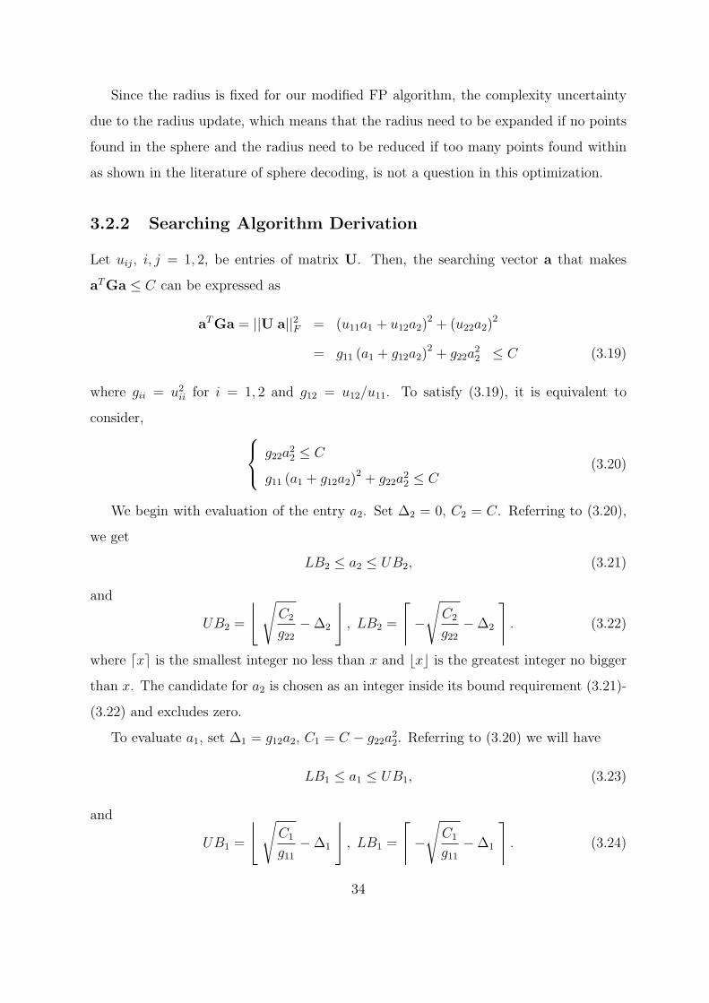
3.2.2 Searching Algorithm Derivation

Let uij, i, j = 1, 2, be entries of matrix U. Then, the searching vector a that makes

aTGa ≤ C can be expressed as

aTGa = ||U a||2F = (u11a1 + u12a2)2 + (u22a2)

2

= g11 (a1 + g12a2)2 + g22a

22 ≤ C (3.19)

where gii = u2ii for i = 1, 2 and g12 = u12/u11. To satisfy (3.19), it is equivalent to

consider, g22a22 ≤ C

g11 (a1 + g12a2)2 + g22a

22 ≤ C

(3.20)

We begin with evaluation of the entry a2. Set ∆2 = 0, C2 = C. Referring to (3.20),

we get

LB2 ≤ a2 ≤ UB2, (3.21)

and

UB2 =

⌊ √C2

g22−∆2

⌋, LB2 =

⌈−

√C2

g22−∆2

⌉. (3.22)

where ⌈x⌉ is the smallest integer no less than x and ⌊x⌋ is the greatest integer no bigger

than x. The candidate for a2 is chosen as an integer inside its bound requirement (3.21)-

(3.22) and excludes zero.

To evaluate a1, set ∆1 = g12a2, C1 = C − g22a22. Referring to (3.20) we will have

LB1 ≤ a1 ≤ UB1, (3.23)

and

UB1 =

⌊ √C1

g11−∆1

⌋, LB1 =

⌈−

√C1

g11−∆1

⌉. (3.24)

34

Then a1 is chosen as an integer inside its bound requirement (3.23)-(3.24) and excludes

zero.

The entries a2, a1 are chosen as follows: for a chosen a2 that satisfies its bound

requirement (3.21)-(3.22) and a2 = 0, we can choose a1 satisfying its bounds requirements

(3.23)-(3.24) and a1 = 0. If such a1 does not exist, we go back and choose other a2. Then

search for a1 that meets its bounds requirement for this new a2 and a1 = 0. When

a set of a2, a1 is chosen, we test the ||a||2 ≤ 1 + P ||h||2 constraint. If satisfied, one

candidate network coding vector a = [a1, a2]T is obtained. We choose the one among all

network coding candidate vectors that gives the smallest aTGametric, which equivalently

maximizes the computation rate at relay R.

Note that this searching procedure will return all candidates that satisfy aTGa ≤ C,

and gives the one with minimum value. There is at least one candidate vector aquant such

that its entries satisfy all the bounds requirements, since that is how we set the radius

value in (3.18). On the other hand, the exhaustive search result aexhaustive that returns

the minimum metric will also fall inside the search bounds, since

aexhaustiveTG aexhaustive ≤ aquant

TG aquant = C. (3.25)

Hence, we are guaranteed to find the optimal exhaustive search result by the proposed

algorithm. Simulation results in Section IV also demonstrate this optimality.

3.2.3 Optimal Network Codes Search Algorithm for TWRC

We summarize our proposed algorithm to search the optimal network coding vector for

TWRC as follows.

Algorithm 3.1 Optimal Network Codes Search Algorithm for TWRC

Input: Channel coefficient vector h.

Output: The optimal network coding vector amin for TWRC.

Step 1: Based on the channel coefficient vector h, construct matrixG asG = I− P(hhT )1+P ||h||2 .

Step 2: Calculate the binary quantized vector obtained by applying the direct sign op-

35

erator of the real minimum-eigenvalue eigenvector of G, denoted as aquant, and set C

as

C = aTquantG aquant. (3.26)

Step 3: Operate Cholesky’s factorization of matrix G, G = UTU. Let uij, i, j = 1, 2

denote the entries of matrix U. Set gii = u2ii for i = 1, 2 and g12 = u12/u11.

Step 4: Search the candidate vector a = [a1, a2]T according to the following procedure.

(i) Initialize ∆2 = 0, C2 = C, metric = C, amin = aquant and k = 2.

(ii) Set the upper bound UBk and the lower bound LBk as follows

UBk =

⌊ √Ck

gkk−∆k

⌋, LBk =

⌈−

√Ck

gkk−∆k

⌉and ak = LBk − 1.

(iii) Set ak = ak + 1. If ak = 0, move to ak = 1. For ak ≤ UBk, go to (v); else go to

(iv).

(iv) If k = 2, terminate and output the searching result amin; else set k = k + 1 and go

to (iii).

(v) For k = 1, go to (vi); else set k = k − 1, and

∆1 = g12a2, C1 = C − g22a22,

then go to (ii).

(vi) Test for ||a||2 ≤ 1 + P ||h||2 constraint to get a candidate vector a. If aTGa ≤

metric, update amin = a and metric = aTGa. Go to (iii).


We present experimental studies to demonstrate the effectiveness of our proposed lemma

and algorithm. First, with the average of 10000 randomly generated channel realizations,

36

we show in Fig. 3.3 that if network coding vector is searched based on general criteria

of theorem 2.3 without our lemma, the probability that the resulting vector will have

at least one zero entry and fails the TWRC system. It can be observed that this issue

is actually very severe. For example, with P ≤ 15dB, the probability of zero entry is

always beyond 1/2.

0 5 10 15 20 25 300.2

0.3

0.4

0.5

0.6

0.7

0.8

0.9

1


Pro

babi

lity

of Z

ero

Ent

ry

Fig. 3.3: Probability of zero entry in TWRC

In Fig. 3.4. we compare the average rate of several strategies under TWRC model.

(i) Relay R decode and transmit x1+x2 to both sources, which we denote as “DF-NC”.

This strategy can been seen as static network coding as it does not consider the channel

variations. (ii) Relay R decode a linear integer combination of both sources, while the

network coding vector are set by simply rounding channel vector h directly, denoted

as “HNC”. (iii) The general CPF scheme while the network coding vector is optimized

without our proposed lemma. We denote as “CPF without zero entry constraints”.

37

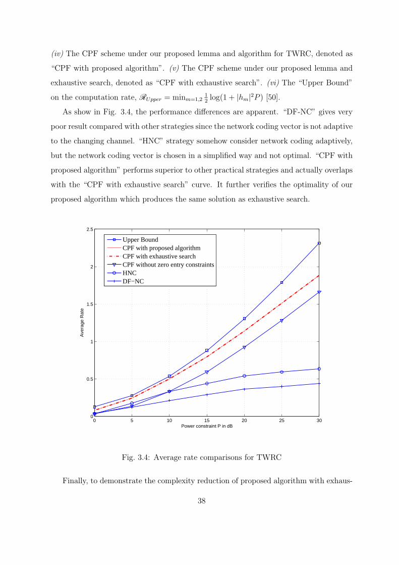
(iv) The CPF scheme under our proposed lemma and algorithm for TWRC, denoted as

“CPF with proposed algorithm”. (v) The CPF scheme under our proposed lemma and

exhaustive search, denoted as “CPF with exhaustive search”. (vi) The “Upper Bound”

on the computation rate, RUpper = minm=1,212log(1 + |hm|2P ) [50].

As show in Fig. 3.4, the performance differences are apparent. “DF-NC” gives very

poor result compared with other strategies since the network coding vector is not adaptive

to the changing channel. “HNC” strategy somehow consider network coding adaptively,

but the network coding vector is chosen in a simplified way and not optimal. “CPF with

proposed algorithm” performs superior to other practical strategies and actually overlaps

with the “CPF with exhaustive search” curve. It further verifies the optimality of our

proposed algorithm which produces the same solution as exhaustive search.

0 5 10 15 20 25 300

0.5

1

1.5

2

2.5


Ave

rage

Rat

e

Upper BoundCPF with proposed algorithmCPF with exhaustive searchCPF without zero entry constraintsHNCDF−NC

Fig. 3.4: Average rate comparisons for TWRC

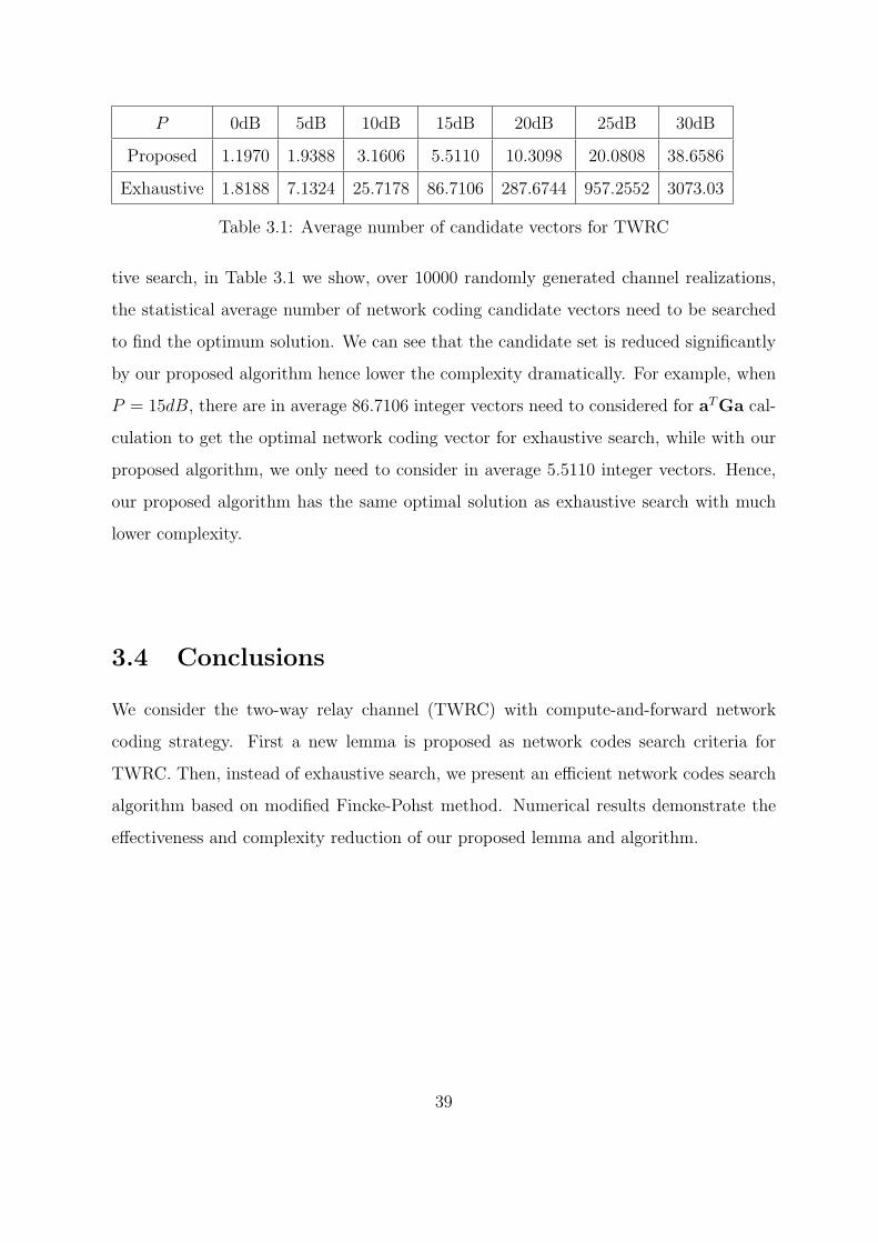
Finally, to demonstrate the complexity reduction of proposed algorithm with exhaus-

38

P 0dB 5dB 10dB 15dB 20dB 25dB 30dB

Proposed 1.1970 1.9388 3.1606 5.5110 10.3098 20.0808 38.6586

Exhaustive 1.8188 7.1324 25.7178 86.7106 287.6744 957.2552 3073.03

Table 3.1: Average number of candidate vectors for TWRC

tive search, in Table 3.1 we show, over 10000 randomly generated channel realizations,

the statistical average number of network coding candidate vectors need to be searched

to find the optimum solution. We can see that the candidate set is reduced significantly

by our proposed algorithm hence lower the complexity dramatically. For example, when

P = 15dB, there are in average 86.7106 integer vectors need to considered for aTGa cal-

culation to get the optimal network coding vector for exhaustive search, while with our

proposed algorithm, we only need to consider in average 5.5110 integer vectors. Hence,

our proposed algorithm has the same optimal solution as exhaustive search with much

lower complexity.

3.4 Conclusions

We consider the two-way relay channel (TWRC) with compute-and-forward network

coding strategy. First a new lemma is proposed as network codes search criteria for

TWRC. Then, instead of exhaustive search, we present an efficient network codes search

algorithm based on modified Fincke-Pohst method. Numerical results demonstrate the

effectiveness and complexity reduction of our proposed lemma and algorithm.

39

Chapter 4

Integer-Forcing Linear Receiver Design with

Slowest Descent Method

4.1 System Model

First we note that it is straightforward that a general complex MIMO system y = Hx+z

can be easily converted into an equivalent real system [62] as Re(y)

Im(y)

=

Re(H) −Im(H)

Im(H) Re(H)

Re(x)

Im(x)

+

Re(z)

Im(z)

. (4.1)

Hence, we will focus on the real MIMO system for analysis convenience.

We consider the classic MIMO channels with L transmit antennas and N receive an-

tennas. Each transmit antenna delivers an independent data stream which is encoded

separately to form the transmitted codewords. We assume that the channel state infor-

mation is only available at the receiver during each transmission. Let L = N for analysis

simplicity.

Without loss of generality, in one transmission realization, each antenna has a length-

k information vectors wm that is drawn independently and uniformly over a prime-size

finite field Fp = 0, 1, · · · , p− 1, i.e.,

wm ∈ Fkp, m = 1, 2, · · · , L. (4.2)

Each antenna is equipped with an encoder Ψm, that maps the length-k messages wm

40

LY

2Y

1Y

M

1w

2w

Lw

)1()( 11 cnc L

)1()( 22 cnc L

)1()(L Lcnc L

1n xx L

1n yy L

Fig. 4.1: MIMO diagram with independent data streams

into the length-n lattice codewords cm ∈ Rn,

Ψm : Fkp → Rn. (4.3)

The codeword satisfies the power constraint of 1n||cm||2 ≤ P , m = 1, · · · , L.

After mapping message wm into a lattice codeword cm with

cm = [cm(1), cm(2), · · · , cm(n)]T , m = 1, · · · , L, (4.4)

antenna m will transmit one information codeword cm in one transmission realization

with a total of n time slots. In the i-th time slot, the transmitted signal vector xi ∈ RL

over L transmit antennas is

xi = [c1(i), c2(i), · · · , cL(i)]T , i = 1, · · · , n. (4.5)

The MIMO system diagram with independent data streams is shown in Fig. 4.1.

Assume a slow fading model where the channel remains constant over the entire

codeword transmission. During one transmission realization, at the ith time slot, i =

1, · · · , n, the received vector yi ∈ RL is,

yi = Hxi + zi, (4.6)

41

where H denotes the L × L channel matrix, with H = [hmj] and hmj is the real valued

fading channel coefficient from transmit antenna j to receive antenna m, and zi ∈ RL

is the additive Gaussian noise. The entries of the channel matrix and the additive noise

vector are generated i.i.d. according to a normal distribution N (0, 1).

To facilitate the detection of desired signals from each antenna, in a linear receiver

architecture, the receiver will project the received vector yi with some matrix B ∈ RL×L

to get the effective received vector for further decoding,

di = Byi = BHxi +Bzi = Axi + ni, (4.7)

where A= BH and ni

= Bzi.

The standard suboptimal linear detection methods include the zero-forcing (ZF) re-

ceiver and the minimum mean square error (MMSE) receiver,

BZF = (HTH)−1HT , (4.8)

BMMSE = (HTH+1

PIL)

−1HT , (4.9)

where (·)T denotes transpose operation and IL is the L×L identity matrix. The ZF tech-

nique nullifies the interference such that AZF = IL with the effect of noise enhancement.

The MMSE receiver maximizes the post-detection signal-to-interference plus noise ratio

(SINR) and mitigates the noise enhancement effects. However, both ZF and MMSE

receiver have been proved to be largely suboptimal in terms of diversity-multiplexing

tradeoff [63].

We recall the important algebraic structure of lattice codes, that the integer com-

bination of lattice codewords is still a codeword. Instead of restricting matrix A to be

identity, we may allow A to be some full rank matrix with integer coefficients, i.e.

AIF ∈ ZL×L. (4.10)

Then we can first separately recover linear combinations of transmitted lattice codewords

with coefficients drawn from matrix AIF, which can be easily solved for the original

messages. Specifically, if

di = [d1(i), d2(i), · · · , dL(i)]T , (4.11)

42

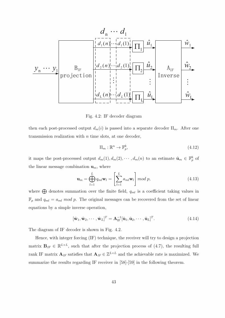
LP

2P

1P

M

1u

2u

Lu

1n yy L

M

1w

2w

Lw

)1()( 11 dnd L

)1()( 22 dnd L

)1()(L Ldnd L

M

1n dd L

Fig. 4.2: IF decoder diagram

then each post-processed output dm(i) is passed into a separate decoder Πm. After one

transmission realization with n time slots, at one decoder,

Πm : Rn → Fkp, (4.12)

it maps the post-processed output dm(1), dm(2), · · · , dm(n) to an estimate um ∈ Fkp of

the linear message combination um, where

um =L⊕l=1

qmlwl =

[L∑l=1

amlwl

]mod p, (4.13)

where⊕

denotes summation over the finite field, qml is a coefficient taking values in

Fp and qml = aml mod p. The original messages can be recovered from the set of linear

equations by a simple inverse operation,

[w1, w2, · · · , wL]T = A−1

IF [u1, u2, · · · , uL]T . (4.14)

The diagram of IF decoder is shown in Fig. 4.2.

Hence, with integer forcing (IF) technique, the receiver will try to design a projection

matrix BIF ∈ RL×L, such that after the projection process of (4.7), the resulting full

rank IF matrix AIF satisfies that AIF ∈ ZL×L and the achievable rate is maximized. We

summarize the results regarding IF receiver in [58]-[59] in the following theorem.

43

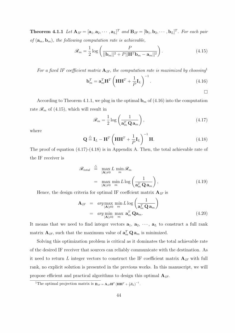
Theorem 4.1.1 Let AIF = [a1, a2, · · · , aL]T and BIF = [b1,b2, · · · ,bL]

T . For each pair

of (am,bm), the following computation rate is achievable,

Rm =1

2log

(P

||bm||2 + P ||HTbm − am||2

). (4.15)

For a fixed IF coefficient matrix AIF, the computation rate is maximized by choosing1

bTm = aT

mHT

(HHT +

1

PIL

)−1

. (4.16)

According to Theorem 4.1.1, we plug in the optimal bm of (4.16) into the computation

rate Rm of (4.15), which will result in

Rm =1

2log

(1

aTmQam

), (4.17)

where

Q= IL −HT

(HHT +

1

PIL

)−1

H. (4.18)

The proof of equation (4.17)-(4.18) is in Appendix A. Then, the total achievable rate of

the IF receiver is

Rtotal= max

|A|=0L min

mRm

= max|A|=0

minm

L log

(1

aTmQam

), (4.19)

Hence, the design criteria for optimal IF coeffcient matrix AIF is

AIF = argmax|A|=0

minm

L log

(1

aTmQam

)= arg min

|A|=0maxm

aTmQam. (4.20)

It means that we need to find integer vectors a1, a2, · · · , aL to construct a full rank

matrix AIF, such that the maximum value of aTm Qam is minimized.

Solving this optimization problem is critical as it dominates the total achievable rate

of the desired IF receiver that sources can reliably communicate with the destination. As

it need to return L integer vectors to construct the IF coefficient matrix AIF with full

rank, no explicit solution is presented in the previous works. In this manuscript, we will

propose efficient and practical algorithms to design this optimal AIF.

1The optimal projection matrix is BIF = AIFHT(HHT + 1

P IL)−1

.

44

4.2 Integer Forcing Linear Receiver Design

To approach the optimization problem of (4.20), first we need to generate some feasible

searching set Ω ⊂ ZL for am ∈ Ω, m = 1, 2, · · · , L, instead of the whole searching space

am ∈ ZL. Then, we will find L linearly independent vectors within this searching set Ω

to construct the optimal IF coefficient matrix AIF.

Accordingly, we propose the following strategy with two steps. In the first step, we

generate the searching set Ω based on slowest descent method [60], which first obtains the

optimal minimizer within the continuous domain, and then finds discrete integer points

with closest Euclidean distance from slowest ascent lines passing through the optimal

continuous minimizer, such that the “good points” with small aT Qa values are within

the candidate set Ω.

In the second step, we pick up a1, a2, · · · , aL ∈ Ω, to construct the full rank IF

coefficient matrix AIF = [a1, a2, · · · , aL]T , while in the meantime, the maximum value

of aTmQam is minimized. Then, equivalently, this optimal AIF will maximize the total

achievable rate.

4.2.1 Candidate Set Searching Algorithm with Slowest Descent

Method

We attempt to find the candidate vector set Ω for a ∈ ZL, a = 0, with small aT Qa values

based on slowest descent method. Note that originally slowest descent method [60] is

presented for maximization problem with “slowest descent” from continuous maximizer.

It can be symmetrically applied to minimization problem with “slowest ascent” from

continuous minimizer. We keep the expression of “slowest descent method” for both

cases.

First, we relax the constraint of a ∈ ZL, a = 0, and assume, instead, that a can be

continuous, real-valued (a ∈ RL) with norm constraint2 ||a|| ≥ 1, then the corresponding

2The integer constraint a ∈ ZL, a = 0 is equivalent to the constraint a ∈ ZL, ||a|| ≥ 1.

45

Fig. 4.3: Creation of one slowest ascent line

optimization problem becomes,

ac = arg mina∈RL,||a||≥1

aTQa. (4.21)

Denote f(a) as the cost function, i.e.,

f(a)= aTQa. (4.22)

Let q1,q2, · · · ,qL be the L normalized eigenvectors of Q with corresponding eigenvalues

λ1 ≤ λ2 ≤ · · · ≤ λL. The real-valued vector for the optimization of (4.21) is well known

and equal to the eigenvector that corresponds to the minimum eigenvalue of matrix Q,

i.e.,

ac = arg mina∈R2L,||a||≥1

f(a) = q1. (4.23)

46

The Hessian of f(a), which is defined as Hfes(a)

= (∂2f(a))/(∂a∂aT ) is

Hfes(a) = (∂2f(a))/(∂a∂aT ) = Q, (4.24)

and well defined at the continuous minimizer vector q1.

Fig. 4.4: The procedure of slowest descent method

Then, the eigenvectors q2, q3, · · · , qL of the Hessian Hfes(a) = Q defines mutually

orthogonal directions of the least ascent in f(a) from the continuous minimizer ac = q1

[60]. Accordingly, we can construct the slowest ascent lines as

L(ρ, i) = q1 + ρqi, ρ ∈ R, i = 2, · · · , L, (4.25)

which pass through the real minimizer ac = q1 with the direction of qi.

The creation of one slowest ascent line q1+ ρqi is shown in Fig. 4.3. We can see that

47

when ρ takes values from (−∞,∞), ρqi is a line in the direction of qi, hence q1 + ρqi is

a line passing through q1 and parallel with the direction of qi.

Those “good” vectors a ∈ Z2L, a = 0 that have small f(a) values stays close to

those slowest ascent lines. Thus, we are trying to identify those vectors that are closest

in Euclidean distance to the above slowest ascent lines, which are the set of candidate

vectors

Ω = a(ρ, i) : ρ ∈ R, i = 2, · · · , L, (4.26)

with

a(ρ, i) = arg mina∈ZL,a=0

||a− L(ρ, i)||. (4.27)

Let M be the bound for searching vector a ∈ ZL in each coordinate, i.e., each co-

ordinate of a takes integer value form [−M,M ]. Denote mj, j = 1, 2, ...2M + 2 as the

midpoints of adjacent discrete points and the bounds of edge points, i.e., mj takes value

from [−M − 12,M + 1

2] with increasing step equal to one. In other words, mj ∈ Λ, where

Λ = −M − 3

2+ j, j = 1, 2, · · · , 2M + 2. (4.28)

For one slowest ascent line q1+ρqi, the closest points to this line changes as ρ varies.

To determine those points, it suffices to find the value of ρ for which a(ρ, i) exhibits a

jump. We may partition the real axis as

(−∞, ρ1], (ρ1, ρ2], · · · , (ρT−1, ρT ], (ρT ,+∞), (4.29)

such that within each interval (ρi, ρi+1], i = 1, · · · , T , there exists exactly one discrete

point a closest to the slowest ascent line.

Denote q1 = [q11, q12, · · · , q1,L]T and qi = [qi1, qi2, · · · , qi,L]T . Then a jump in one

component of a(ρ, i) occurs when ρ takes the following value,

ρ′(j−1)∗L+k =mj − q1k

qik, (4.30)

with k = 1, · · · , L, and j = 1, · · · , 2M + 2.

After sorting the ρ′1, ρ′2, · · · , ρ′(2M+2)×2L calculated from (4.30) in ascending order,

we will get the ρ1, ρ2, · · · , ρT for the partition of (4.29) with T ≤ (2M + 2)× 2L.

48

Now that we have those intervals for ρ, we are ready to find the points closest to the

slowest ascent line q1 + ρqi. For one interval (ρj, ρj+1], j = 1, · · · , T − 1, we can let ρ

take the value of

ρ =1

2(ρj + ρj+1), (4.31)

and calculate the closest point a(ρj ,ρj+1],i by rounding to the closest integer point as

a(ρj ,ρj+1],i = round

(q1 +

1

2(ρj + ρj+1)qi

). (4.32)

After searching through all T − 1 intervals of ρ, we clear the points beyond the bounds

[−M,M ] in any coordinate, excludes the zero vector3 and put all the final validate points

that closest to one slowest ascent line q1 + ρqi in the set of Ωi−1, i ∈ 2, · · · , L.

Finally, for J slowest ascent lines, 1 ≤ J ≤ L− 1, we obtain the candidate vector set

Ω = Ω1

∪Ω2

∪· · ·∪

ΩJ . (4.33)

The procedure of slowest descent method is shown in Fig. 4.4. In this example, the

bound for searching vector a in each coordinate isM = 2, i.e., each coordinate takes value

from [−2,−1, 0, 1, 2]. mj, j = 1, 2, · · · , 6 is among Λ = [−2.5,−1.5,−0.5, 0.5, 1.5, 2.5].

There exists a jump in one component of searching vector a when ρ takes value in

some interval edge such that the slowest ascent line q1 + ρqi passes the dark solid dots.

Within two dark solid dots, there exists only one point closest to the slowest ascent line.

After proceeding the described slowest descent method, the outcome candidate points

are shown with red solid points.

The complexity reduction of our proposed algorithm for candidate vector set algorith-

m based on slowest descent method with direct exhaustive search is remarkable. Even

when we restrict the direct exhaustive search among the same bound [−M,M ] in every

coordinate for the searching vector, the direct exhaustive search will need to consider

(2M + 1)L searching vectors, which is exponential to L. While with our proposed algo-

rithm with slowest descent method, we only need to consider T ≤ (2M + 2) × L points

for each slowest ascent line. For J slowest ascent lines, the total vectors considered will

3We add the zero points to facilitate the searching. At the end of the procedure, the vector with

all-zero coordinates will exclude.

49

be less than (2M + 2)J × L. Simulation will show that only a few slowest descent lines

need to be considered. Hence, the total complexity of proposed algorithm for candidate

vector set algorithm based on slowest descent method will be polynomial to L.

We summarize our proposed algorithm for candidate vector set Ω search based on

slowest descent method as follows.

Algorithm 4.1 Candidate Set Search Algorithm with Slowest Descent Method

Input: Matrix Q, the bound for each coordinate M , and the

number of slowest descent lines J .

Output: The searching vector candidate set Ω.

Step 1: Calculate the eigenvectors q1,q2,· · · ,qL of matrix Q with corresponding eigen-

values λ1 ≤ λ2 ≤ · · · ≤ λL.

Step 2: Compute the set of Λ which mj, j = 1, 2, ...2M + 2 takes value from,

Λ = −M − 3

2+ j, j = 1, 2, · · · , 2M + 2. (4.34)

Step 3: For i = 2, · · · , J + 1 (1 ≤ J ≤ L− 1), do

(i) Obtain the jumping points where ρ takes value as

ρ′(j−1)∗L+k =mj − q1k

qik,

with k = 1, · · · , L, j = 1, · · · , 2M + 2.

(ii) Sort ρ′1, ρ′2, · · · , ρ′(2M+2)×L in ascending order into ρ1, ρ2, · · · , ρT .

(iii) For each interval (ρj, ρj+1], j = 1, · · · , T − 1, we take the value of ρ as

ρ =1

2(ρj + ρj+1),

and calculate the closest point a(ρj ,ρj+1],i as

a(ρj ,ρj+1],i = round

(q1 +

1

2(ρj + ρj+1)qi

).

50

(iv) Clear the points beyond the bounds [−M,M ] in any coordinate, excludes the zero

vector and put all the final validate points that closest to one slowest ascent line

q1 + ρqi in set Ωi−1.

Step 3: After searching along J slowest ascent lines, we obtain

Ω = Ω1

∪Ω2

∪· · ·∪

ΩJ . (4.35)

4.2.2 Constructing IF Coefficient Matrix AIF

According to our proposed candidate set search algorithm with slowest descent method,

we get the feasible searching set Ω for IF vectors a1, a2, · · · , aL. With function f(·)

defined in (4.22), we sort all vectors within the candidate set Ω such that

Ω = t1, t2, · · · , t|Ω| : f(t1) ≤ f(t2) ≤ · · · ≤ f(t|Ω|). (4.36)

We are trying to choose L linear independent vectors within this sorted set by

a1 = ti1 , a2 = ti2 , · · · , aL = tiL , for some i1 < i2 < · · · < iL, (4.37)

then the constructed IF coefficient matrixAIF has full rank L. We will select a1, a2, · · · , aL

in Ω based on the greedy search algorithm [53].

The procedure try to find a1, a2, · · · , aL sequentially and is described as follows,

a1 = t1

a2 = argmint∈Ω

f(t) | t, a1 are linearly independent

a3 = argmint∈Ω

f(t) | t, a1, a2 are linearly independent...

aL = argmint∈Ω

f(t) | t, a1, · · · , aL−1 are linearly independent

We summarize this procedure to constructing the full rank optimal matrix AIF with

candidate vector set Ω as follows.

51

Algorithm 4.2 IF Coefficient Matrix Constructing with Greedy Search Algorithm

Input: Searching set Ω, Matrix Q.

Output: The IF coefficient matrix AIF with full rank that gives

the maximum total achievable rate Rtotal.

Step 1: Let f(t) = tTQt and sort all vectors in the searching candidate set Ω such that

Ω = t1, t2, · · · , t|Ω| : f(t1) ≤ f(t2) ≤ · · · ≤ f(t|Ω|).

Set a1 = t1. Initialize i = 1 and j = 1.

Step 2: While i < |Ω| and j < L, do

(i) Set i = i+ 1.

(ii) If ti, a1,· · · ,aj are linearly independent, then:

Set j = j + 1,

aj = ti.

Else goto Step 2.

Step 3: Construct the full rank IF coefficient matrix A as A = [a1, a2, · · · , aL]T .


We present numerical results to evaluate the performance of our proposed algorithm for

IF receiver design. First, we discuss the IF performance with respect to some parameters.

One of them is J , which represents how many slowest ascent lines are chosen during the

candidate set search procedure. For an example setting with L = 8, which J can take

values in [1, 2, · · · , 7], we average over 10000 randomly generated channel realizations and

show the average rate in Fig. 4.5. The bound for each coordinate of searching vector is

M = 2. We can see that as J increases, since the candidate set Ω = Ω1

∪Ω2 · · ·

∪ΩJ will

expand, the performance is getting better as expected. However, we do not need to span

52

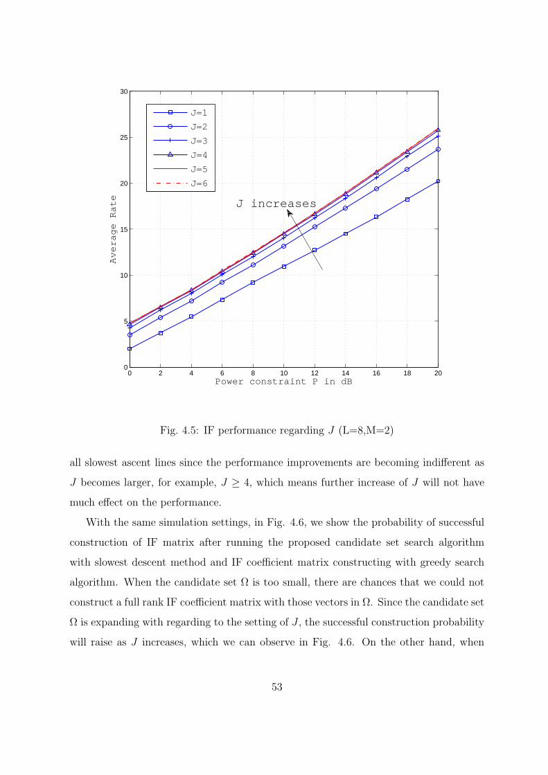
0 2 4 6 8 10 12 14 16 18 200

5

10

15

20

25

30


Average Rate

J=1

J=2

J=3

J=4

J=5

J=6

J increases

Fig. 4.5: IF performance regarding J (L=8,M=2)

all slowest ascent lines since the performance improvements are becoming indifferent as

J becomes larger, for example, J ≥ 4, which means further increase of J will not have

much effect on the performance.

With the same simulation settings, in Fig. 4.6, we show the probability of successful

construction of IF matrix after running the proposed candidate set search algorithm

with slowest descent method and IF coefficient matrix constructing with greedy search

algorithm. When the candidate set Ω is too small, there are chances that we could not

construct a full rank IF coefficient matrix with those vectors in Ω. Since the candidate set

Ω is expanding with regarding to the setting of J , the successful construction probability

will raise as J increases, which we can observe in Fig. 4.6. On the other hand, when

53

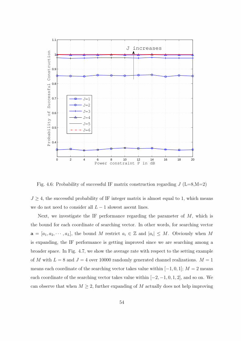
0 2 4 6 8 10 12 14 16 18 20

0.4

0.5

0.6

0.7

0.8

0.9

1

1.1


Probability of Successful Construction

J=1

J=2

J=3

J=4

J=5

J=6

J increases

Fig. 4.6: Probability of successful IF matrix construction regarding J (L=8,M=2)

J ≥ 4, the successful probability of IF integer matrix is almost equal to 1, which means

we do not need to consider all L− 1 slowest ascent lines.

Next, we investigate the IF performance regarding the parameter of M , which is

the bound for each coordinate of searching vector. In other words, for searching vector

a = [a1, a2, · · · , aL], the bound M restrict ai ∈ Z and |ai| ≤ M . Obviously when M

is expanding, the IF performance is getting improved since we are searching among a

broader space. In Fig. 4.7, we show the average rate with respect to the setting example

of M with L = 8 and J = 4 over 10000 randomly generated channel realizations. M = 1

means each coordinate of the searching vector takes value within [−1, 0, 1]; M = 2 means

each coordinate of the searching vector takes value within [−2,−1, 0, 1, 2], and so on. We

can observe that when M ≥ 2, further expanding of M actually does not help improving

54

0 2 4 6 8 10 12 14 16 18 200

5

10

15

20

25

30


Average Rate

M=1

M=2

M=3

M=4

M increases

Fig. 4.7: IF performance regarding M (L=8,J=4)

the performance any more. This is because those “good” vectors a ∈ ZL, a = 0 that have

small aTQa values stay close to the continuous minimizer (4.23) and tends to have small

coordinates. As shown in Fig. 4.7, M = 2 is good enough for this setting example. Hence,

for different settings, we can investigate and decide the proper J and M parameters for

further realizations.

After the parameters setting discussion, we are ready to compare the performance

of different linear detection methods. The standard linear detection methods of ZF and

MMSE are included for comparisons. We also take account in the channel capacity of

C = 12log det(IL+PHHT ), which represents the upper bound for all receiver structures,

linear or non-linear including joint ML. In Fig. 4.8, we show the rate comparisons over

MIMO channels with L = 4, J = 2, M = 2 and average of 10000 randomly generated

55

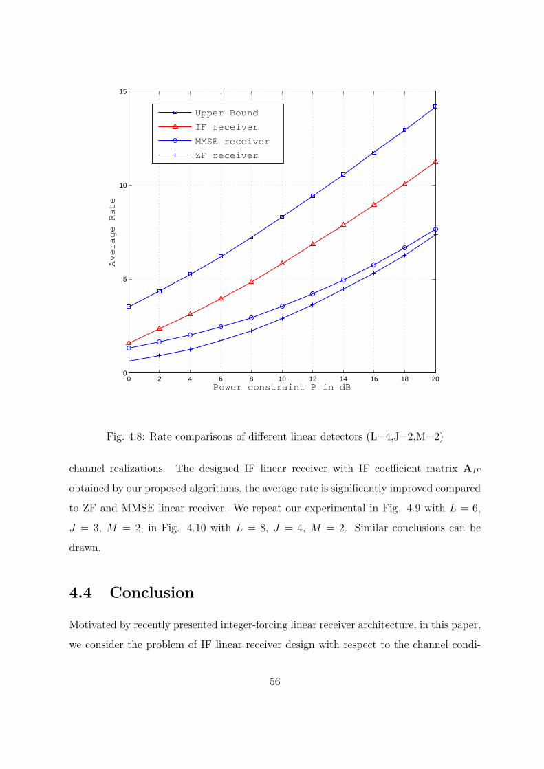
0 2 4 6 8 10 12 14 16 18 200

5

10

15


Average Rate

Upper Bound

IF receiver

MMSE receiver

ZF receiver

Fig. 4.8: Rate comparisons of different linear detectors (L=4,J=2,M=2)

channel realizations. The designed IF linear receiver with IF coefficient matrix AIF

obtained by our proposed algorithms, the average rate is significantly improved compared

to ZF and MMSE linear receiver. We repeat our experimental in Fig. 4.9 with L = 6,

J = 3, M = 2, in Fig. 4.10 with L = 8, J = 4, M = 2. Similar conclusions can be

drawn.

4.4 Conclusion

Motivated by recently presented integer-forcing linear receiver architecture, in this paper,

we consider the problem of IF linear receiver design with respect to the channel condi-

56

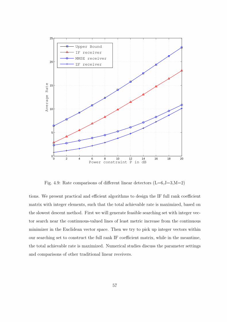
0 2 4 6 8 10 12 14 16 18 200

5

10

15

20

25


Average Rate

Upper Bound

IF receiver

MMSE receiver

ZF receiver


tions. We present practical and efficient algorithms to design the IF full rank coefficient

matrix with integer elements, such that the total achievable rate is maximized, based on

the slowest descent method. First we will generate feasible searching set with integer vec-

tor search near the continuous-valued lines of least metric increase from the continuous

minimizer in the Euclidean vector space. Then we try to pick up integer vectors within

our searching set to construct the full rank IF coefficient matrix, while in the meantime,

the total achievable rate is maximized. Numerical studies discuss the parameter settings

and comparisons of other traditional linear receivers.

57

0 2 4 6 8 10 12 14 16 18 200

5

10

15

20

25

30

35


Average Rate

Upper Bound

IF receiver

MMSE receiver

ZF receiver


4.5 Appendix

Proof of Equations (4.17)-(4.18)

Denote L = 1

P||bm||2 + ||HTbm − am||2, then

L =1

PbTmbm + bT

mHHTbm − aTmH

Tbm − bTmHam + aT

mam.

Let F = HHT + 1

PIL. Accordingly the optimal bT

m can be written as

bTm = aT

mHT

(HHT +

1

PIL

)−1

= aTmH

TF−1.

58

Plug in this optimal bTm in L, we have

L = aTm

HTF−1

Pbm + aT

mHTF−1HHTbm − aT

mHTbm

−aTmH

TF−1Ham + aTmam

= aTmH

TF−1

(1

PIL +HHT

)︸︷︷︸

F

bm − aTmH

Tbm

−aTmH

TF−1Ham + aTmam

= aTmam − aT

mHTF−1Ham

= aTm

(IL −HTF−1H

)︸︷︷︸Q

am.

Hence, the computation rate

Rm =1

2log

(P

||bm||2 + P ||HTbm − am||2

)=

1

2log

(1

L

)=

1

2log

(1

aTmQam

),

where

Q = IL −HTF−1H

= IL −HT

(HHT +

1

PIL

)−1

H.

59

Chapter 5

Network Coding in Wireless Cooperative

Networks with Multiple Antenna Relays

In this Chapter, we consider network coding application in wireless multiple access relay

channels. Four system models are considered:

(i) System model A: Two sources without direct links;

(ii) System model B: Two sources with direct links;

(iii) System model C: Three sources with direct links;

(iv) System model D: Four sources with direct links.

5.1 System Model A: Two Sources Without Direct

Links

Consider cooperative system with two sources: multiple access relay channels without

direct links. Two sources S1, S2 communicate with destination D via a relay R without

direct links from sources to destination, as shown in Fig. 5.1. We assume the sources S1,

S2 and the destination D are equipped with single antenna, while relay R is equipped

with two antennas.

The information transmission is performed in two phases with three time slots in

total. In the first phase two source nodes transmit simultaneously to relay R in one time

60

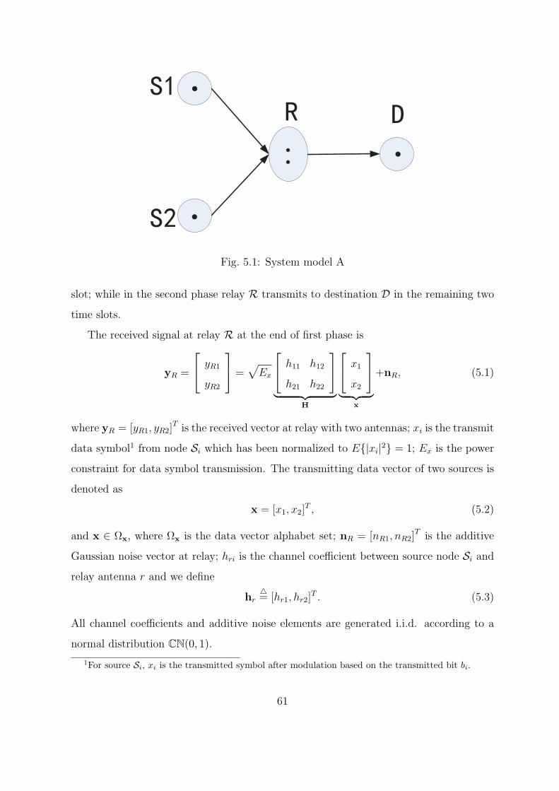
Fig. 5.1: System model A

slot; while in the second phase relay R transmits to destination D in the remaining two

time slots.

The received signal at relay R at the end of first phase is

yR =

yR1

yR2

=√

Ex

h11 h12

h21 h22

︸︷︷︸

H

x1

x2

︸︷︷︸

x

+nR, (5.1)

where yR = [yR1, yR2]T is the received vector at relay with two antennas; xi is the transmit

data symbol1 from node Si which has been normalized to E|xi|2 = 1; Ex is the power

constraint for data symbol transmission. The transmitting data vector of two sources is

denoted as

x = [x1, x2]T , (5.2)

and x ∈ Ωx, where Ωx is the data vector alphabet set; nR = [nR1, nR2]T is the additive

Gaussian noise vector at relay; hri is the channel coefficient between source node Si and

relay antenna r and we define

hr= [hr1, hr2]

T . (5.3)

All channel coefficients and additive noise elements are generated i.i.d. according to a

normal distribution CN(0, 1).1For source Si, xi is the transmitted symbol after modulation based on the transmitted bit bi.

61

In the second phase, relay R will transmit to the destination D according to differ-

ent schemes. As no direct links exist in system model A, physical layer network coding

(PLNC) cannot be applied in system model A directly. Note that all schemes take three

time slots for one transmission realization.

5.1.1 Different Schemes for System Model A

(i) System Model A Scheme 1: Decode-and-Forward (DF)

With this scheme, after receiving yR in (5.1), relay R will first decode for two sources

xR =

xR1

xR2

= arg minx∈Ωx

||yR −√ExHx||2. (5.4)

Then, relay R will transmit xR1 and xR2 in two time slots as follows,

yD =√ER

xR1 0

0 xR2

g1

g2

+ nD

=√ER

g1 0

0 g2

︸︷︷︸

G1

xR1

xR2

+ nD, (5.5)

which is equivalent to

yD =√

ERG1xR + nD, (5.6)

where gr, r = 1, 2 is the channel coefficient between relay antenna r and destination D.

The decoding procedure at destination D will be

x = arg minx∈Ωx

||yD −√ERG1x||2. (5.7)

(ii) System Model A Scheme 2: Space Time Decode-and-Forward (STDF)

In this scheme, relay R will first decode for two sources the same way as scheme 1,

equation (5.4), then transmit xR1 and xR2 according to Alamouti space time coding [68].

62

In the second time slot, the relay will transmit [xR1, xR2]T and in the third time

slot, the relay will transmit [−x∗R2, x

∗R1]

T . Denote the corresponding received signals at

destination D in the second phase (with two time slots) as yD1 and yD2, then

[yD1, yD2] =√

ER [g1, g2]

xR1 −x∗R2

xR2 x∗R1

+ [nD1, nD2]. (5.8)

After receiving signals from relay R in the second phase, destination D arranges the

received signals into a vector yD = [yD1,−y∗D2]T , which can be rewritten as

yD =

yD1

−y∗D2

=

√ER

g1 g2

−g∗2 g∗1

︸︷︷︸

G2

xR1

xR2

+ nD

=√ERG2xR + nD, (5.9)

where nD = [nD1,−n∗D2]

T .


x = arg minx∈Ωx

||yD −√ERG2x||2. (5.10)

(iii) System Model A Scheme 3: Analog Network Coding (ANC)

In this scheme, relay R will utilize analog network coding to process the received

signals. First, after receiving yR of (5.1), relay R constructs the following signal vector

t = [t1, t2]T based on the received signals on each antenna

t =

β1yR1

β2yR2

=

β1 0

0 β2

︸︷︷︸

B

(√

ExHx+ nR), (5.11)

where βr, r = 1, 2 is the scaling factor to meet the per-antenna power constraint PR at

relay R given by

βr =

√1

E|yRr|2=

√1

Ex||hr||2 + 1. (5.12)

63

Then, relay R will transmit t1 and t2 in two time slots as follows,

yD =√

ER

t1 0

0 t2

g1

g2

+ nD

=√

ER

g1 0

0 g2

︸︷︷︸

G1

t1

t2

+ nD

=√

ER

√ExG1BHx+

√ERG1BnR + nD. (5.13)


x = arg minx∈Ωx

||yD −√

ER

√ExG1BHx||2. (5.14)

(iv) System Model A Scheme 4: Space Time Analog Network Coding (S-

TANC)

In this scheme, we consider combine analog network coding with Alamouti space time

coding. After constructing t = [t1, t2]T as equation (5.11), relay R will transmit [t1, t2]

T

in the second time slot and [−t∗2, t∗1]

T in the third time slot. Denote the corresponding

received signals at destination D in the second phase (with two time slots) as yD1 and

yD2, then

[yD1, yD2] =√

ER [g1, g2]

t1 −t∗2

t2 t∗1

+ [nD1, nD2], (5.15)

where gr, r = 1, 2 is the channel coefficient between relay antenna r and destination D.


received signals into a vector yD = [yD1,−y∗D2]T , which can be rewritten as

yD =

yD1

−y∗D2

=

√ER

g1 g2

−g∗2 g∗1

︸︷︷︸

G2

t1

t2

+ nD

=√

ER

√ExG2BHx+

√ERG2BnR + nD, (5.16)

64

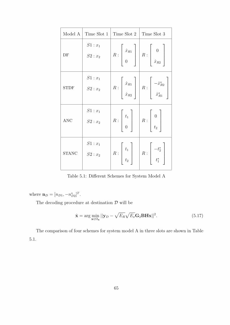
Model A Time Slot 1 Time Slot 2 Time Slot 3

DF

S1 : x1

S2 : x2R :

xR1

0

R :

0

xR2

STDF

S1 : x1

S2 : x2R :

xR1

xR2

R :

−x∗R2

x∗R1

ANC

S1 : x1

S2 : x2R :

t1

0

R :

0

t2

STANC

S1 : x1

S2 : x2R :

t1

t2

R :

−t∗2

t∗1

Table 5.1: Different Schemes for System Model A

where nD = [nD1,−n∗D2]

T .


x = arg minx∈Ωx

||yD −√

ER

√ExG2BHx||2. (5.17)

The comparison of four schemes for system model A in three slots are shown in Table

5.1.

65

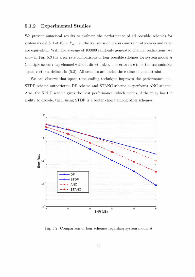
5.1.2 Experimental Studies

We present numerical results to evaluate the performance of all possible schemes for

system model A. Let Ex = ER, i.e., the transmission power constraint at sources and relay

are equivalent. With the average of 100000 randomly generated channel realizations, we

show in Fig. 5.3 the error rate comparisons of four possible schemes for system model A

(multiple access relay channel without direct links). The error rate is for the transmission

signal vector x defined in (5.2). All schemes are under three time slots constraint.

We can observe that space time coding technique improves the performance, i.e.,

STDF scheme outperforms DF scheme and STANC scheme outperforms ANC scheme.

Also, the STDF scheme gives the best performance, which means, if the relay has the

ability to decode, then, using STDF is a better choice among other schemes.

5 10 15 20 25 3010

−4

10−3

10−2

10−1

100

SNR (dB)

Err

or R

ate

DF

STDF

ANC

STANC

Fig. 5.2: Comparison of four schemes regarding system model A

66

5.2 SystemModel B: Two Sources With Direct Links

Consider cooperative system model B: multiple access relay channels with direct links.

Two sources S1, S2 communicate with destination D via relay R with direct links from

sources to destination, as shown in Fig. 5.2. We also assume the sources S1, S2 and

the destination D are equipped with single antenna, while relay R is equipped with two

antennas.

Fig. 5.3: System model B

One realization of the information transmission is performed in two time slots. We

will describe in details the different four possible schemes, which all take two time slots

for one transmission realization. Since we constrain the transmission is performed within

two time slots, space-time coding cannot be directly applied to system model B directly.

5.2.1 Different Schemes for System Model B

(i) System Model B Scheme 1: Direct Transmission (DT)

In this scheme, we assume the relay will keep silent during all transmission realization

and the sources will communicate to the destination one by one directly. S1 will transmit

67

in the first time slot; S2 will transmit in the second time slot.

yD1 =√Exf1x1 + nD1,

yD2 =√Exf2x2 + nD2,

which can be combined to yD = [yD1, yD2]T as

yD =√Ex

f1 0

0 f2

︸︷︷︸

F

x1

x2

︸︷︷︸

x

+

nD1

nD2

︸︷︷︸

nD

, (5.18)

or equivalently

yD =√

ExFx+ nD. (5.19)

fi is the direct link channel coefficient between source Si to destination D; nDi is the

additive Gaussian noise at the i-th time slot. All channel coefficients are generated i.i.d.

according to a normal distribution N (0, 1).

Hence the decoding procedure at destination D will be

x = arg minx∈Ωx

||yD −√

ExFx||2. (5.20)

(ii) System Model B Scheme 2: Decode-and-Forward (DF)

In this scheme, two sources will transmit to relay R and destination D simultaneously

in the first time slot, while in the second time slot relay R will transmit the decoded

signals to destination D.

The received signal at destination D at the end of first time slot is

yD1 =√

Exf1x1 +√

Exf2x2 + nD1. (5.21)

The received vector at relay R with two antennas at the end of first time slot is

yR =√

Ex

h11 h12

h21 h22

︸︷︷︸

H

x1

x2

+

nR1

nR2

, (5.22)

68

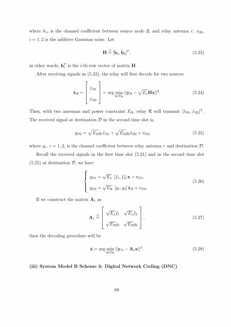
where hri is the channel coefficient between source node Si and relay antenna r; nRi,

i = 1, 2 is the additive Gaussian noise. Let

H= [h1,h2]

T , (5.23)

in other words, hTi is the i-th row vector of matrix H.

After receiving signals as (5.22), the relay will first decode for two sources

xR =

xR1

xR2

= arg minx∈Ωx

||yR −√ExHx||2. (5.24)

Then, with two antennas and power constraint ER, relay R will transmit [xR1, xR2]T .

The received signal at destination D in the second time slot is,

yD2 =√

ERg1xR1 +√

ERg2xR2 + nD2. (5.25)

where gr, r = 1, 2, is the channel coefficient between relay antenna r and destination D.

Recall the received signals in the first time slot (5.21) and in the second time slot

(5.25) at destination D, we haveyD1 =

√Ex [f1, f2]x+ nD1,

yD2 =√ER [g1, g2] xR + nD2.

(5.26)

If we construct the matrix A1 as

A1=

√Exf1

√Exf2

√ERg1

√ERg2

, (5.27)

then the decoding procedure will be

x = arg minx∈Ωx

||yD −A1x||2. (5.28)

(iii) System Model B Scheme 3: Digital Network Coding (DNC)

69

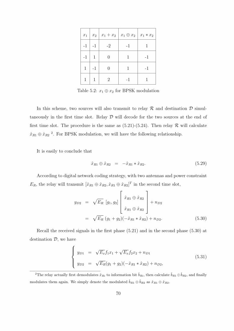
x1 x2 x1 + x2 x1 ⊕ x2 x1 ∗ x2

-1 -1 -2 -1 1

-1 1 0 1 -1

1 -1 0 1 -1

1 1 2 -1 1

Table 5.2: x1 ⊕ x2 for BPSK modulation

In this scheme, two sources will also transmit to relay R and destination D simul-

taneously in the first time slot. Relay D will decode for the two sources at the end of

first time slot. The procedure is the same as (5.21)-(5.24). Then relay R will calculate

xR1 ⊕ xR22. For BPSK modulation, we will have the following relationship.

It is easily to conclude that

xR1 ⊕ xR2 = −xR1 ∗ xR2. (5.29)

According to digital network coding strategy, with two antennas and power constraint

ER, the relay will transmit [xR1 ⊕ xR2, xR1 ⊕ xR2]T in the second time slot,

yD2 =√ER [g1, g2]

xR1 ⊕ xR2

xR1 ⊕ xR2

+ nD2

=√ER (g1 + g2)(−xR1 ∗ xR2) + nD2. (5.30)

Recall the received signals in the first phase (5.21) and in the second phase (5.30) at

destination D, we haveyD1 =

√Exf1x1 +

√Exf2x2 + nD1

yD2 =√ER(g1 + g2)(−xR1 ∗ xR2) + nD2,

(5.31)

2The relay actually first demodulates xRi to information bit bRi, then calculate bR1⊕ bR2, and finally

modulates them again. We simply denote the modulated bR1 ⊕ bR2 as xR1 ⊕ xR2.

70

and will decode x = [x1, x2]T as

x = argminx1,x2 ||yD1 −√Exf1x1 −

√Exf2x2||2

+||yD2 +√ER (g1 + g2)(x1 ∗ x2)||2. (5.32)

(iv) System Model B Scheme 4: Analog Network Coding (ANC)


signals. First, after receiving yR of (5.22), relayR constructs the signal vector t = [t1, t2]T

as follows,

t =

β1yR1

β2yR2

=

β1 0

0 β2

︸︷︷︸

B

(√

ExHx+ nR), (5.33)

where βr, r = 1, 2 is the scaling factor at relay R given by

βr =

√1

E|yRr|2=

√1

Ex||hr||2 + 1. (5.34)

Then, relay R will transmit t1, t2 in the second time slot as follows,

yD2 =√

ER[g1, g2]

t1

t2

+ nD2

=√

ER

√Exg

TBHx+√

ERgTBnR + nD2, (5.35)

where

g= [g1, g2]

T , (5.36)

is the channel vector between relay R with two antennas to destination D.

Combining the received signals in the first time slot (5.21) and in the second time

slot (5.35) at destination D, with f= [f1, f2]

T , we have

yD =√Ex

fT

√ERg

TBH

︸︷︷︸

A2

x+

nD1

√ERg

TBnR + nD2

︸︷︷︸

z

. (5.37)

71

Model B Time Slot 1 Time Slot 2

DT S1 : x1 S2 : x2

DF

S1 : x1

S2 : x2R :

xR1

xR2

DNC

S1 : x1

S2 : x2R :

xR1 ⊕ xR2

xR1 ⊕ xR2

ANC

S1 : x1

S2 : x2R :

t1

t2

Table 5.3: Different Schemes for System Model B

which can be decoded as

x = arg minx∈Ωx

||yD −A2x||2. (5.38)

The comparison of four schemes for system model B in three slots are shown in Table

5.3.



system model B. Let Ex = ER, i.e., the transmission power constraint at sources and

relay are equivalent. With the average of 100000 randomly generated channel realizations,

the error rate comparison of all possible schemes for system model B is given in Fig. 5.4.

All schemes are under two time slots constraint. Interestingly, we find that the schemes

72

of DNC and ANC both give inferior performance to the simply DF scheme, which means,

when relay is equipped with multiple antennas, simply transmit decoded messages onto

different antennas outperforms mixing signals as in DNC and ANC schemes.

5 10 15 20 25 3010

−3

10−2

10−1

100

SNR (dB)

Err

or R

ate

DTDFDNCANC

Fig. 5.4: Comparison of four schemes regarding system model B

5.3 SystemModel C: Three Sources with Direct Links

Consider the system model setting with three sources S1, S2, S3 communicating with

destination D via a relay R, with direct links from sources to destination, as shown in

Fig. 5.5. We assume sources S1, S2, S3 and destination D are equipped with single

antenna, while relay R is equipped with two antennas.

We will discuss several possible transmission strategies for this system model. One

realization of the information transmission will be performed within three time slots for

73

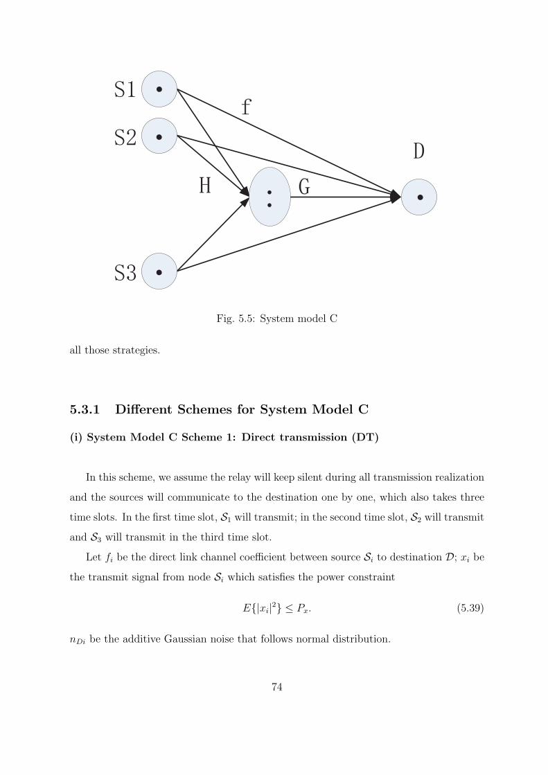
Fig. 5.5: System model C

all those strategies.

5.3.1 Different Schemes for System Model C

(i) System Model C Scheme 1: Direct transmission (DT)


and the sources will communicate to the destination one by one, which also takes three

time slots. In the first time slot, S1 will transmit; in the second time slot, S2 will transmit

and S3 will transmit in the third time slot.

Let fi be the direct link channel coefficient between source Si to destination D; xi be

the transmit signal from node Si which satisfies the power constraint

E|xi|2 ≤ Px. (5.39)

nDi be the additive Gaussian noise that follows normal distribution.

74

Then, the received signals at destination D during three time slots are

yD1 = f1x1 + nD1, (5.40)

yD2 = f2x2 + nD2, (5.41)

yD3 = f3x3 + nD3, (5.42)

which can be combined to

yDT =

yD1

yD2

yD3

=

f1 0 0

0 f2 0

0 0 f3

︸︷︷︸

ADT

x1

x2

x3

︸︷︷︸

x

+

nD1

nD2

nD3

︸︷︷︸

zDT

. (5.43)

Note that x is the transmit data vector of three sources x= [x1, x2, x3]

T and

x ∈ Ωx, (5.44)

where Ωx is the data vector alphabet set. Hence the decoding procedure for DT scheme

will simply be

xDT = arg minx∈Ωx

||yDT −ADTx||2. (5.45)

The sum rate at destination D for DT scheme will be

RDT =1

3log det

(I3 + PxADTA

HDT

). (5.46)

The one-third factor above is the natural consequence of time sharing.

(ii) System Model C Scheme 2: Analog Network Coding (ANC)

Regarding this scheme, in the first phase all source nodes transmit simultaneously to

relay R and destination D in one time slot; while the second phase is the transmission

from relay R to destination D during the remaining two time slots.

75

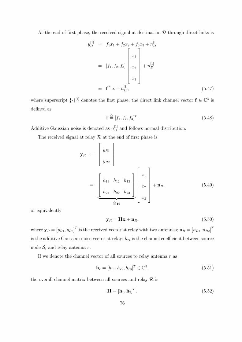
At the end of first phase, the received signal at destination D through direct links is

y[1]D = f1x1 + f2x2 + f3x3 + n

[1]D

= [f1, f2, f3]

x1

x2

x3

+ n[1]D

= fT x+ n[1]D , (5.47)

where superscript ·[1] denotes the first phase; the direct link channel vector f ∈ C3 is

defined as

f= [f1, f2, f3]

T . (5.48)

Additive Gaussian noise is denoted as n[1]D and follows normal distribution.

The received signal at relay R at the end of first phase is

yR =

yR1

yR2

=

h11 h12 h13

h21 h22 h23

︸︷︷︸

= H

x1

x2

x3

+ nR, (5.49)

or equivalently

yR = Hx+ nR, (5.50)

where yR = [yR1, yR2]T is the received vector at relay with two antennas; nR = [nR1, nR2]

T

is the additive Gaussian noise vector at relay; hri is the channel coefficient between source

node Si and relay antenna r.

If we denote the channel vector of all sources to relay antenna r as

hr = [hr1, hr2, hr3]T ∈ C3, (5.51)

the overall channel matrix between all sources and relay R is

H = [h1,h2]T . (5.52)

76

All channel coefficients and additive noise elements are generated i.i.d. according to a

normal distribution CN (0, 1).

In the second phase, first, relay R constructs the following signal vector t based on

the received signals on each antenna (yR1 and yR2),

t =

t1

t2

=

β1yR1

β2yR2

=

β1 0

0 β2

︸︷︷︸

= B

(Hx+ nR). (5.53)

where βr, r = 1, 2 is the scaling factor to meet the per-antenna power constraint PR at

relay R given by

βr =

√PR

E|yRr|2

=

√PR

Px||hr||2 + 1. (5.54)

Then, relay R will transmit t1 and t2 in two time slots as follows,

[y[2]D (1), y

[2]D (2)

]= [g1, g2]

t1 0

0 t2

+ [n[2]D (1), n

[2]D (2)], (5.55)

where superscript ·[2] denotes the first phase; gr, r = 1, 2, is the channel coefficient

between relay antenna r and destination D.

Equivalently, equation (5.55) can be written as

y[2]D =

y[2]D (1)

y[2]D (2)

=

g1 0

0 g2

t1

t2

+ n[2]D

= G0t+ n[2]D , (5.56)

where matrix G0 is defined as

G0=

g1 0

0 g2

, (5.57)

77

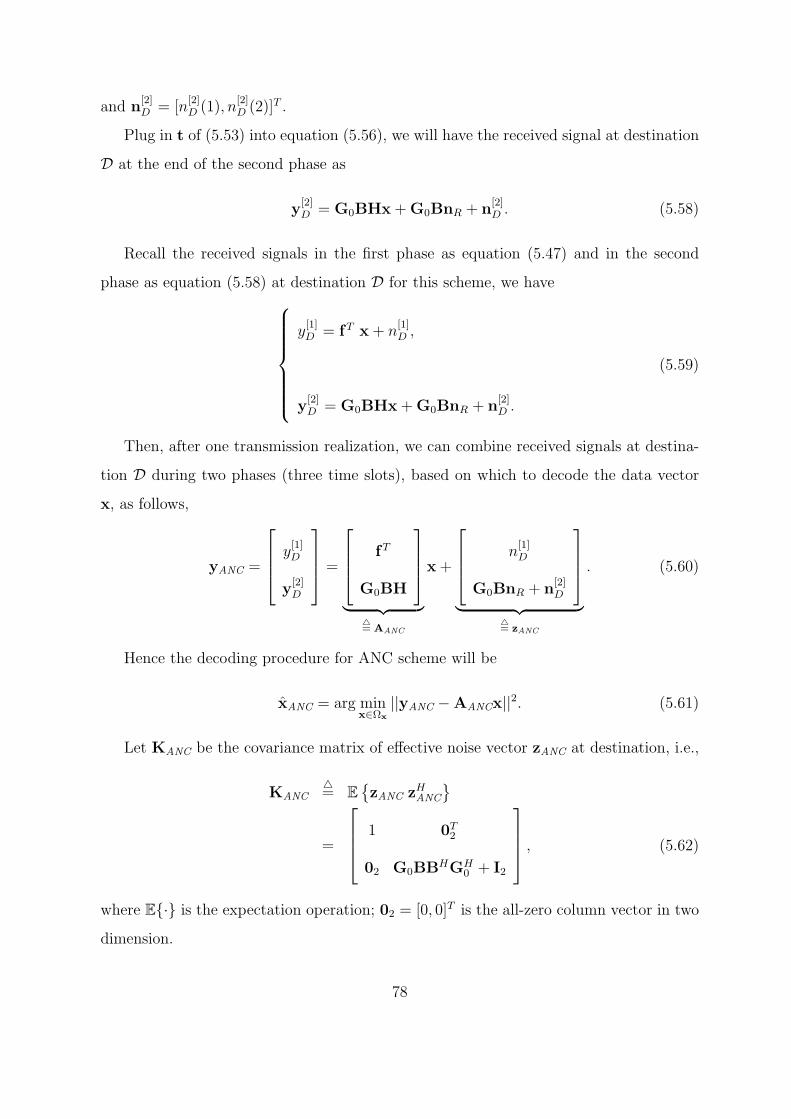
and n[2]D = [n

[2]D (1), n

[2]D (2)]T .

Plug in t of (5.53) into equation (5.56), we will have the received signal at destination

D at the end of the second phase as

y[2]D = G0BHx+G0BnR + n

[2]D . (5.58)

Recall the received signals in the first phase as equation (5.47) and in the second

phase as equation (5.58) at destination D for this scheme, we havey[1]D = fT x+ n

[1]D ,


[2]D .

(5.59)

Then, after one transmission realization, we can combine received signals at destina-

tion D during two phases (three time slots), based on which to decode the data vector

x, as follows,

yANC =

y[1]D

y[2]D

=

fT

G0BH

︸︷︷︸

= AANC

x+

n[1]D

G0BnR + n[2]D

︸︷︷︸

= zANC

. (5.60)

Hence the decoding procedure for ANC scheme will be

xANC = arg minx∈Ωx

||yANC −AANCx||2. (5.61)

Let KANC be the covariance matrix of effective noise vector zANC at destination, i.e.,

KANC= E

zANC zHANC

=

1 0T2

02 G0BBHGH0 + I2

, (5.62)

where E· is the expectation operation; 02 = [0, 0]T is the all-zero column vector in two

dimension.

78

The sum rate at destination D for ANC scheme will be

RANC =1

3log det

(I3 + Px AANC AH

ANC K−1ANC

). (5.63)

(iii) System Model C Scheme 3: Space-Time Analog Network Coding with

Alamouti (STANC-Alamouti)

In this scheme, the first transmission phase will be the same as in ANC scheme. In

other words, at the end of first phase, the received signal at the destination D will be as

equation (5.47) and the received signals at the relay R will be as equation (5.50).

After constructing the signal vector t as equation (5.53), relay R will combine analog

network coding with Alamouti scheme. According to Alamouti scheme, after obtaining

t = [t1, t2]T , relay R will transmit [t1, t2]

T in the second time slot and [−t∗2, t∗1]

T in the

third time slot.

Denote the corresponding received signals at destination D in the second phase (with

two time slots) as y[2]D (1) and y

[2]D (2), then

[y[2]D (1), y

[2]D (2)

]= [g1, g2]

t1 −t∗2

t2 t∗1

+ [n[2]D (1), n

[2]D (2)]. (5.64)

Destination D arranges the received signals into a vector y[2]D =

[y[2]D (1),−y

[2]D (2)∗

]T,

which can be rewritten as

y[2]D =

y[2]D (1)

−y[2]D (2)∗

=

g1 g2

−g∗2 g∗1

t1

t2

+ n[2]D

= G1t+ n[2]D , (5.65)

where matrix G1 is defined as

G1=

g1 g2

−g∗2 g∗1

, (5.66)

79

and n[2]D = [n

[2]D (1),−n

[2]D (2)∗]T .

Plug in t of (5.53) into equation (5.56), we will have the received signal at destination

D at the end of the second phase as


[2]D . (5.67)

Recall the received signals in the first phase as equation (5.47) and in the second

phase as equation (5.67) at destination D for this scheme, we havey[1]D = fT x+ n

[1]D ,


[2]D .

(5.68)

Finally, after one transmission realization, we combine received signals at destination

D based on which to decode the data vector x, during two phases (three time slots) as

ySTANC =

y[1]D

y[2]D

=

fT

G1BH

︸︷︷︸

= ASTANC

x+

n[1]D

G1BnR + n[2]D

︸︷︷︸

= zSTANC

. (5.69)

The decoding procedure can be expressed as

xSTANC = arg minx∈Ωx

||ySTANC −ASTANCx||2. (5.70)

Let KSTANC be the covariance matrix of effective noise vector zSTANC at destination,

i.e.,

KSTANC= E

zSTANC zHSTANC

=

1 0T2

02 G1BBHGH1 + I2

. (5.71)

The sum rate at destination D for STANC scheme will be

RSTANC =1

3log det

(I3 + Px ASTANC AH

STANC K−1STANC

). (5.72)

The comparison of different schemes within three slots are shown in Table 5.4.

80

System Model C Time Slot 1 Time Slot 2 Time Slot 3

DT S1 : x1 S2 : x2 S3 : x3

ANC

S1 : x1

S2 : x2

S3 : x3

R :

t1

0

R :

0

t2

STANC-Alamouti

S1 : x1

S2 : x2

S3 : x3

R :

t1

t2

R :

−t∗2

t∗1

Table 5.4: Different Schemes for System Model C



MARC system model. Let Px = PR, i.e., the transmission power constraint at sources and

relay are equivalent. With the average of 100000 randomly generated channel realizations,

we show in Fig. 5.6 the sum rate comparisons of three possible schemes. We can see that

STANC outperforms the other two schemes unless the signal power is extremely low.

The bit error rate simulation is shown in Fig. 5.7. Similar conclusions can be drawn.

5.4 System Model D: Four Sources with Direct Links

Consider the system model setting with four sources S1, S2, S3 and S4 communicating

with destination D via a relay R with direct links from sources to destination, as shown

in Fig. 5.9. We assume that the sources S1, S2, S3, S4 and the destination D are equipped

with single antenna, while relay R is equipped with two antennas.

We will discuss several possible transmission strategies for this system model. One

realization of the information transmission will be performed within four time slots for

all those strategies.

81

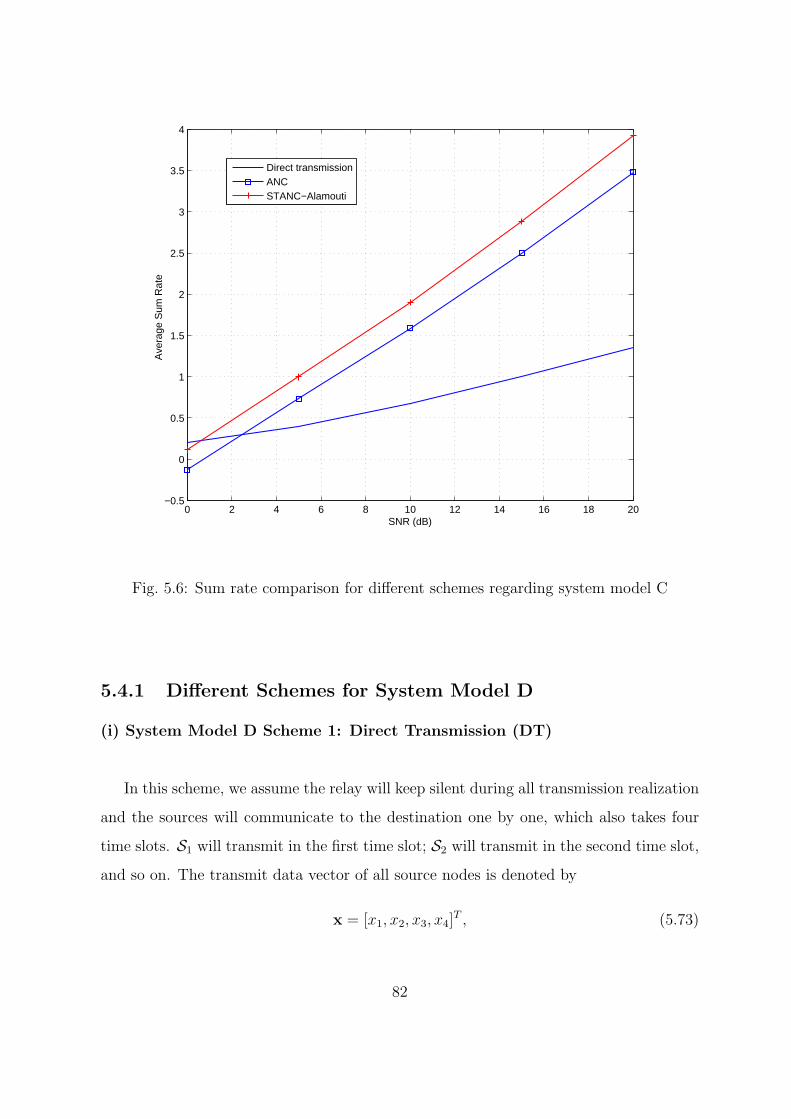
0 2 4 6 8 10 12 14 16 18 20−0.5

0

0.5

1

1.5

2

2.5

3

3.5

4

SNR (dB)

Ave

rage

Sum

Rat

e

Direct transmissionANCSTANC−Alamouti

Fig. 5.6: Sum rate comparison for different schemes regarding system model C

5.4.1 Different Schemes for System Model D

(i) System Model D Scheme 1: Direct Transmission (DT)


and the sources will communicate to the destination one by one, which also takes four

time slots. S1 will transmit in the first time slot; S2 will transmit in the second time slot,

and so on. The transmit data vector of all source nodes is denoted by

x = [x1, x2, x3, x4]T , (5.73)

82

0 2 4 6 8 10 12 14 16 18 2010

−5

10−4

10−3

10−2

10−1

100

SNR (dB)

Err

or R

ate

Direct transmissionANCSTANC−Alamouti

Fig. 5.7: BER comparison for different schemes regarding system model C

where xi ∈ R is the transmit data symbol3 from node Si which has been normalized to

E|xi|2 ≤ 1. Ex is the power constraint for data symbol transmission. Let fi ∈ R be

the direct link channel coefficient between source Si to destination D, an independent

Gaussian random variable with variance σ2f . Additive Gaussian noise follows normal

distribution N (0, 1).

Then, the received signals at the destination D during the four time slots can be

3For source Si, xi is the transmitted symbol after modulation based on the transmitted bit bi, where

bi ∈ 0, 1.

83

Fig. 5.8: System Model D

combined to yD = [yD1, yD2, yD3, yD4]T as

yD =√

Ex

f1 0 0 0

0 f2 0 0

0 0 f3 0

0 0 0 f4

︸︷︷︸

ADT

x1

x2

x3

x4

︸︷︷︸

x

+

nD1

nD2

nD3

nD4

︸︷︷︸

z

, (5.74)

or equivalently

yD = ADTx+ z. (5.75)

Note that x is the transmit data vector of four sources and x ∈ Ωx, where Ωx is the

data vector alphabet set. Hence the decoding procedure will simply be

x = arg minx∈Ωx

||yD −ADTx||2. (5.76)

(ii) System Model D Scheme 2: Decode-and-Forward (DF)

84

In this scheme, one realization of the information transmission is performed in two

phases. The first phase (with two time slots) is the transmission from sources to relay

R. We first separate the four sources into two groups. S1, S2 belong to one group and

S3, S4 belong to another group. In the first time slot, sources S1 and S2 will transmit to

the relay; while in the second time slot, sources S3 and S4 will transmit to the relay. The

second phase (also with two time slots) is the transmission from relay R to destination

D.

In the first phase, the received signals at destination D at the end of first time slot

and second time slot are

y[1]D (1) =

√Exf1x1 +

√Exf2x2 + n

[1]D (1) (5.77)

y[1]D (2) =

√Exf3x3 +

√Exf4x4 + n

[1]D (2) (5.78)

where the superscript ·[1] denotes the first phase. We can rewrite (5.77) and (5.78) into

y[1]D =

√Ex

f1 f2 0 0

0 0 f3 f4

︸︷︷︸

F

x1

x2

x3

x4

+ n

[1]D , (5.79)

where y[1]D = [y

[1]D (1), y

[1]D (2)]T ; n

[1]D is i.i.d. Gaussian noise with normal distribution.

The received signals at relay R at the end of first time slot and second time slot are

y(1)R =

√Ex

h11 h12

h21 h22

x1

x2

+

nR1

nR2

, (5.80)

y(2)R =

√Ex

h13 h14

h23 h24

x3

x4

+

nR3

nR4

, (5.81)

where y(1)R is the received vector at relay with two antennas in the first time slot and y

(2)R

is the received vector at relay with two antennas in the second time slot; nRi, i = 1, 2, 3, 4

is the additive Gaussian noise; hri is the channel coefficient between source node Si and

85

relay antenna r, an independent Gaussian random variable with variance σ2h. Additive

noise elements are generated i.i.d. according to a normal distribution N (0, 1).

With equations (5.80) and (5.81), we can easily obtain

yR =

y(1)R

y(2)R

=

yR1

yR2

yR3

yR4

=√

Ex

h11 h12 0 0

h21 h22 0 0

0 0 h13 h14

0 0 h23 h24

︸︷︷︸

H

x1

x2

x3

x4

︸︷︷︸

x

+

nR1

nR2

nR3

nR4

︸︷︷︸

nR

,

(5.82)

or equivalently

yR =√

ExHx+ nR, (5.83)

which is the received signal at relay R at the end of first transmission phase.

In the second phase, with the decode-and-forward (DF) scheme, relay R will first

decode for four sources

xR =

xR1

xR2

xR3

xR4

= arg min

x∈Ωx

||yR −√ExHx||2. (5.84)

Then, with two antennas and power constraint ER, relay R will transmit [xR1, xR2]T in

the third time slot and transmit [xR3, xR4]T in the fourth time slot with two antennas.

The received signals at destination D at the end of third time slot and fourth time

86

slot are

y[2]D (1) =

√ERg1xR1 +

√ERg2xR2 + n

[2]D (1) (5.85)

y[2]D (2) =

√ERg1xR3 +

√ERg2xR4 + n

[2]D (2), (5.86)

where the superscript ·[2] denotes the second phase. gr, r = 1, 2, is the channel co-

efficient between relay antenna r and destination D, an independent Gaussian random

variable with variance σ2g . Additive Gaussian noise elements are generated i.i.d. according

to a normal distribution N (0, 1). We can rewrite (5.85) and (5.86) into

y[2]D =

√ER

g1 g2 0 0

0 0 g1 g2

︸︷︷︸

G

xR + n[2]D . (5.87)

With the received signals in the first phase (5.79) and in the second phase (5.87) at

destination D, we have

y[1]D =

√Ex

f1 f2 0 0

0 0 f3 f4

x+ n[1]D

=√ExFx+ n

[1]D ,

y[2]D =

√ER

g1 g2 0 0

0 0 g1 g2

xR + n[2]D

=√ERGxR + n

[2]D .

(5.88)

If we construct the matrix ADF as

ADF=

√ExF

√ERG

, (5.89)

then the decoding procedure will be

x = arg minx∈Ωx

||yD −ADFx||2. (5.90)

87

We note that in this DF scheme, the system model with four sources is actually

equivalent to two separate multiple access relay channels (MARC) with two sources.

Each separate MARC system is working in two time slots. For example, for a sub-system

with sources S1 and S2 in Fig. 2, in the first time slot, S1 and S2 transmit simultaneously;

in the second time slot, relay R will forward the decoded x1 and x2 with two antennas.

3x

1x

2x

4x

Fig. 5.9: The equivalent two separate MARC with two sources for DF

(iii) System Model D Scheme 3: Digital Network Coding (DNC)

In this scheme, the first transmission phase will be the same as in the decode-and-

forward scheme. In other words, at the end of first phase, the received signals at the

destination D will be (5.79) and the received signals at the relay R will be (5.82)-(5.83).

Then, relay R will first decode for four sources the same way as the DF scheme,

88

equation (5.84) and formulate xR1 ⊕ xR2, xR3 ⊕ xR44.

It can be denoted as

xR1 ⊕ xR2 = −xR1 ∗ xR2 (5.91)

xR3 ⊕ xR4 = −xR3 ∗ xR4. (5.92)

According to digital network coding strategy, with two antennas and power constraint

ER, the relay will transmit [xR1 ⊕ xR2, xR1 ⊕ xR2]T and [xR3 ⊕ xR4, xR3 ⊕ xR4]

T in the

following two time slots,

[y[2]D (1), y

[2]D (2)] =

√ER [g1, g2]

xR1 ⊕ xR2 xR3 ⊕ xR4

xR1 ⊕ xR2 xR3 ⊕ xR4

+ [n

[2]D (1), n

[2]D (2)],

which can be arranged as

y[2]D =

√ER

g1 + g2 0

0 g1 + g2

xR1 ⊕ xR2

xR3 ⊕ xR4

+ n[2]D . (5.93)



y[1]D =

√Ex

f1 f2 0 0

0 0 f3 f4

x+ n[1]D = Fx+ n

[1]D ,

y[2]D =

√ER

g1 + g2 0

0 g1 + g2

xR1 ⊕ xR2

xR3 ⊕ xR4

+ n[2]D .

(5.94)

we can easily see that, according to this DNC scheme, the system is actually equivalent

to two separate multiple access relay channels (MARC) with two sources as in Fig. 3.

4The relay actually first demodulates xRi to information bit bRi, then calculate bR1 ⊕ bR2, bR3 ⊕ bR4,

and finally modulates them again. We simply denote the modulated bR1 ⊕ bR2, bR3 ⊕ bR4 as xR1 ⊕ xR2,

xR3 ⊕ xR4.

89

Each two sources MARC system is working in two time slots, while in the first time slot

sources transmitting and in the second time slot the relay will forward the XOR symbol

of the decoded messages.

2

1

ˆ

ˆ

x

xÅ

4

3

ˆ

ˆx

xÅ

Fig. 5.10: The equivalent two separate MARC with two sources for DNC

The decoding procedure can also be processed according to those two separate MARC

system. For sources S1 and S2, we have y[1]D (1) =

√Exf1x1 +

√Exf2x2 + n

[1]D (1)

y[2]D (1) =

√ER(g1 + g2)(−xR1 ∗ xR2) + n

[2]D (1),

(5.95)

90

and will decode [x1, x2]T as x1

x2

= argminx1,x2 ||y[1]D (1)−

√Exf1x1 −

√Exf2x2||2

+||y[2]D (1) +√ER(g1 + g2)(x1 ∗ x2)||2. (5.96)

For sources S3 and S4 we can decode in a similar way, x3

x4

= argminx3,x4 ||y[1]D (2)−

√Exf3x3 −

√Exf4x4||2

+||y[2]D (2) +√ER(g1 + g2)(x3 ∗ x4)||2. (5.97)

(iv) System Model D Scheme 4: Dignal Network Coding with Alamouti space

time coding (DNC-Alamouti)

In this scheme, the first transmission phase will also be the same as in the decode-

and-forward scheme. In other words, at the end of first phase, the received signals at the

destination D will be (5.79) and the received signals at the relay R will be (5.82)-(5.83).

Then, relay R will first decode for four sources the same way as the DF scheme,

equation (5.84) and formulate xR1 ⊕ xR2 and xR3 ⊕ xR4. The transmission from relay

R will follow the Alamouti space time coding. In the third time slot, the relay will

transmit [xR1 ⊕ xR2, xR3 ⊕ xR4]T and in the fourth time slot, the relay will transmit

[−(xR3 ⊕ xR4)∗, (xR1 ⊕ xR2)

∗]T . Denote the corresponding received signals at destination

D in the second phase (with two time slots) as y[2]D (1) and y

[2]D (2), then

[y[2]D (1), y

[2]D (2)

]=

√ER[g1, g2]

xR1 ⊕ xR2 −(xR3 ⊕ xR4)∗

xR3 ⊕ xR4 (xR1 ⊕ xR2)∗

+ [n[2]D (1), n

[2]D (2)].(5.98)


received signals into a vector y[2]D =

[y[2]D (1),−y

[2]D (2)∗

]T, which can be rewritten as

y[2]D =

y[2]D (1)

−y[2]D (2)∗

=√ER

g1 g2

−g∗2 g∗1

xR1 ⊕ xR2

xR3 ⊕ xR4

+ n[2]D , (5.99)

91

where n[2]D = [n

[2]D (1),−n

[2]D (2)∗]T .



y[1]D =

√Ex

f1 f2 0 0

0 0 f3 f4

x+ n[1]D = Fx+ n

[1]D ,

y[2]D =

√ER

g1 g2

−g∗2 g∗1

xR1 ⊕ xR2

xR3 ⊕ xR4

+ n[2]D .

(5.100)

Equivalently, the received signals at destination during the two phases can be written

as

yD1 =√Exf1x1 +

√Exf2x2 + nD1

yD2 =√Exf3x3 +

√Exf4x4 + nD2

yD3 = −√ERg1(xR1 ∗ xR2)−

√ERg2(xR3 ∗ xR4) + nD3

yD4 =√ERg

∗2(xR1 ∗ xR2)−

√ERg

∗1(xR3 ∗ xR4) + nD4,

where [yD1, yD2, yD3, yD4] = [(y[1]D )T , (y

[2]D )T ] and [nD1, nD2, nD3, nD4] = [(n

[1]D )T , (n

[2]D )T ].

The correspondent decoding procedure will be

x = arg minx1,x2,x3,x4

||yD1 −√

Exf1x1 −√Exf2x2||2 + ||yD2 −

√Exf3x3 −

√Exf4x4||2

+||yD3 +√ERg1(xR1 ∗ xR2) +

√ERg2(xR3 ∗ xR4)||2

+||yD4 −√

ERg∗2(xR1 ∗ xR2) +

√ERg

∗1(xR3 ∗ xR4)||2. (5.101)

(v) System Model D Scheme 5: Analog Network Coding (ANC)


signals. First, after receiving yR of (5.82)-(5.83), relay R constructs the following signal

92

vector

t =

t1

t2

t3

t4

=

β1yR1

β2yR2

β3yR3

β4yR4

=

β1 0 0 0

0 β2 0 0

0 0 β3 0

0 0 0 β

︸︷︷︸

B

(√

ExHx+ nR), (5.102)

where βr, r = 1, 2, 3, 4 is the scaling factor at relay R given by

βr =

√1

E|yRr|2=

√1

Ex||hr||2 + 1. (5.103)

Note that hTr is the r-th row vector of matrix H in (5.82), i.e.,

H = [h1,h2,h3,h4]T . (5.104)

Then, relay R will transmit t1, t2, t3 and t4 in two time slots as follows,

[y[2]D (1), y

[2]D (2)

]=√

ER [g1, g2]

t1 t3

t2 t4

+ [n[2]D (1), n

[2]D (2)], (5.105)

which can be arranged as

y[2]D =

y[2]D (1)

y[2]D (2)

=√

ER

g1 g2 0 0

0 0 g1 g2

︸︷︷︸

G

t1

t2

t3

t4

+ n

[2]D

=√

ER

√ExGBHx+

√ERGBnR + n

[2]D . (5.106)

Combining the received signals in the first phase (5.79) and in the second phase

(5.106) at destination D, we have

yD =√Ex

F

√ERGBH

︸︷︷︸

AANC

x+

n[1]D

√ERGBnR + n

[2]D

︸︷︷︸

z

. (5.107)

93

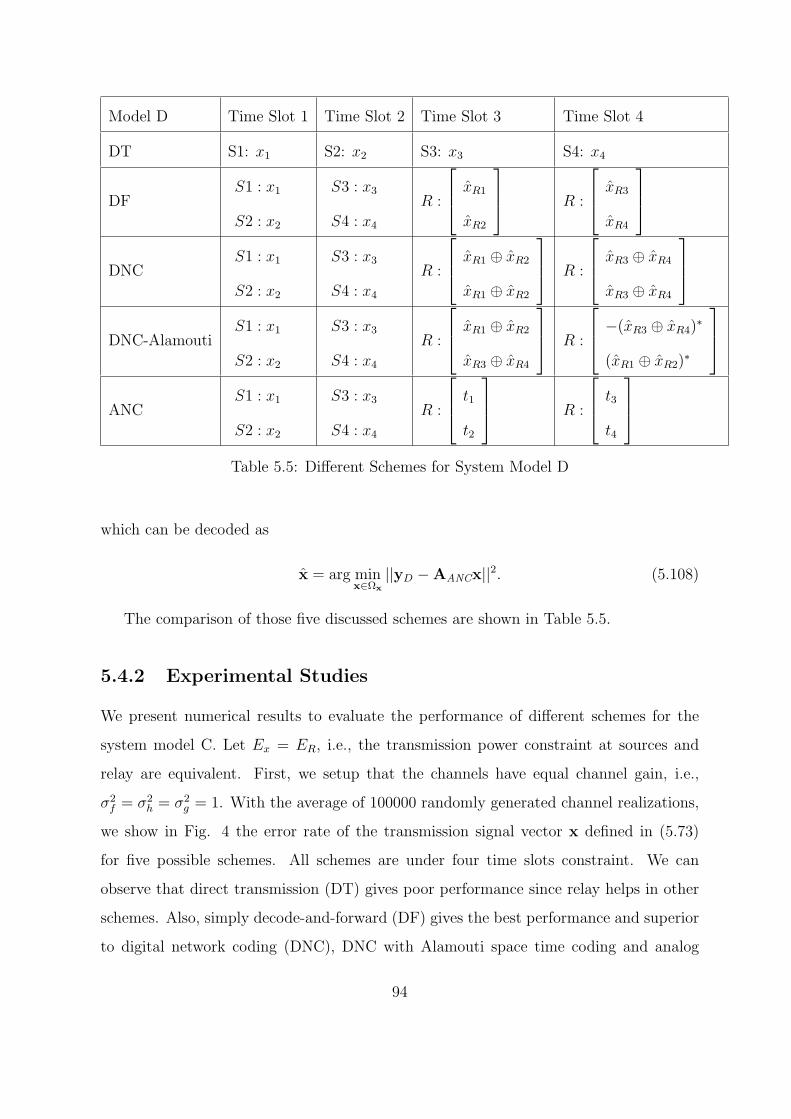
Model D Time Slot 1 Time Slot 2 Time Slot 3 Time Slot 4

DT S1: x1 S2: x2 S3: x3 S4: x4

DFS1 : x1

S2 : x2

S3 : x3

S4 : x4

R :

xR1

xR2

R :

xR3

xR4

DNC

S1 : x1

S2 : x2

S3 : x3

S4 : x4

R :

xR1 ⊕ xR2

xR1 ⊕ xR2

R :

xR3 ⊕ xR4

xR3 ⊕ xR4

DNC-Alamouti

S1 : x1

S2 : x2

S3 : x3

S4 : x4

R :

xR1 ⊕ xR2

xR3 ⊕ xR4

R :

−(xR3 ⊕ xR4)∗

(xR1 ⊕ xR2)∗

ANC

S1 : x1

S2 : x2

S3 : x3

S4 : x4

R :

t1

t2

R :

t3

t4

Table 5.5: Different Schemes for System Model D

which can be decoded as

x = arg minx∈Ωx

||yD −AANCx||2. (5.108)

The comparison of those five discussed schemes are shown in Table 5.5.


We present numerical results to evaluate the performance of different schemes for the

system model C. Let Ex = ER, i.e., the transmission power constraint at sources and

relay are equivalent. First, we setup that the channels have equal channel gain, i.e.,

σ2f = σ2

h = σ2g = 1. With the average of 100000 randomly generated channel realizations,

we show in Fig. 4 the error rate of the transmission signal vector x defined in (5.73)

for five possible schemes. All schemes are under four time slots constraint. We can

observe that direct transmission (DT) gives poor performance since relay helps in other

schemes. Also, simply decode-and-forward (DF) gives the best performance and superior

to digital network coding (DNC), DNC with Alamouti space time coding and analog

94

5 10 15 20 25 3010

−3

10−2

10−1

100

Ex (dB)

Err

or R

ate

of T

rans

mis

sion

Sig

nal V

ecto

r

DT

DF

DNC

DNC−Alamouti

ANC

Fig. 5.11: Comparison of five schemes regarding system model D, σ2f = σ2

h = σ2g = 1

network coding (ANC). A rough explanation about this may be that in the DF case,

each relay antenna has a clean decoded signal to transmit, while in schemes with network

coding each relay antenna is transmitting a mixed decoded signals, which degrades the

performance.

Then, we investigate the performance of all possible schemes with some extreme chan-

nel gain setup. For example, if the direct links from sources to destination have the worst

channel with σ2f = 0.1, σ2

h = σ2g = 1, we show the error rate of the transmission signal

vector comparisons in Fig. 5. We can see that DF still gives best performance, while

DT, DNC and DNC-Alamouti schemes suffers more since they rely on the information

transmitted on the direct links more.

Another extreme channel gain setup is that the links between the sources and the

relay have the worst conditions amongst all, i.e., σ2h = 0.1, σ2

f = σ2g = 1. In this case, the

95

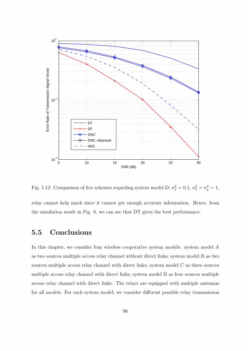
5 10 15 20 25 3010

−2

10−1

100

SNR (dB)

Err

or R

ate

of T

rans

mis

sion

Sig

nal V

ecto

r

DT

DF

DNC

DNC−Alamouti

ANC

Fig. 5.12: Comparison of five schemes regarding system model D: σ2f = 0.1, σ2

h = σ2g = 1,

relay cannot help much since it cannot get enough accurate information. Hence, from

the simulation result in Fig. 6, we can see that DT gives the best performance.

5.5 Conclusions

In this chapter, we consider four wireless cooperative system models: system model A

as two sources multiple access relay channel without direct links; system model B as two

sources multiple access relay channel with direct links; system model C as three sources

multiple access relay channel with direct links; system model D as four sources multiple

access relay channel with direct links. The relays are equipped with multiple antennas

for all models. For each system model, we consider different possible relay transmission

96

5 10 15 20 25 3010

−2

10−1

100

SNR (dB)

Err

or R

ate

of T

rans

mis

sion

Sig

nal V

ecto

r

DT

DF

DNC

DNC−Alamouti

ANC

Fig. 5.13: Comparison of five schemes regarding system model D: σ2h = 0.1, σ2

f = σ2g = 1

schemes, including possibly combining network coding and space-time coding techniques.

We find that under three time slots constraint, space-time decode-and-forward (STD-

F) gives superior performance than decode-and-forward (DF), analog network coding

(ANC) and space-time analog network coding (STANC) schemes for system model A;

while under two time slots constraint, the simply decode-and-forward (DF) scheme out-

performs the direct transmission, physical layer network coding (PLNC) and anolog net-

work coding (ANC) schemes for system model B.

Regarding system model C, with three time constraints, traditional relay transmis-

sion schemes are not directly applicable. We discuss DT, ANC and STANC-Alamouti

schemes. Simulation studies show that STANC with alamouti scheme outperform other

schemes regarding sum rate and bit error rate performance at the destination.

Regarding system model D, we investigate several schemes for the system model under

97

four time slots transmission constraint, describe in details those different schemes and

compare the error rate performance. Interestingly, simulation studies show that those

schemes with network coding have not better performance than the traditional schemes,

which indicates that network coding is not favorable for the system model if traditional

schemes can also be implemented with the same time slots constraint.

98

Bibliography

[1] L. Wei and W. Chen, “Compute-and-forward network coding design over multi-

source multi-relay channels”, IEEE Trans. Wireless Communications, vol. 11, no. 9,

pp. 3348-3357, Sept. 2012.

[2] L. Wei and W. Chen, “Efficient compute-and-forward network codes search for two-

way relay channel”, IEEE Commun. Letters, vol. 16, no. 8, pp. 1204-1207, Aug. 2012.

[3] L. Wei and W. Chen, “Optimal binary/quaternary adaptive signature design for

code-division multiplexing”, IEEE Trans. Wireless Communications, accepted, 2012.

[4] L. Wei and D. A. Pados, “Optimal orthogonal carriers and sum-SINR/sum-capacity

of the multiple-access vector channel”, IEEE Trans. Communications, vol. 60, no. 5,

pp. 1188-1192, May 2012.

[5] L. Wei and W. Chen, “Optimal upward scaling of minimum-TSC binary signature

sets”, IEEE Commun. Letters, vol. 16, no. 2, pp. 168-171, Feb. 2012.

[6] L. Wei, S. N. Batalama, D. A. Pados and B. W. Suter, “Adaptive binary signature

design for code division multiplexing”, IEEE Trans. Wireless Communications, vol.

7, no. 7, pp. 2798-2804, July 2008.

[7] L. Wei, S. N. Batalama, D. A. Pados, and B. W. Suter, “Upward scaling of minimum-

TSC binary signature sets”, IEEE Commun. Letters, vol. 11, no. 11, pp. 889-891, Nov.

2007.

99

[8] Y. Yu, W. Chen and L. Wei, “Design of convergence-optimized non-binary LDPC

codes over binary erasure channel”, IEEE Wireless Commun. Letters, vol. 1, no. 4,

pp. 336-339, Aug. 2012.

[9] Y. Wei, Y. Yang, L. Wei and W. Chen, “Comments on A new parity-check stopping

criterion for turbo decoding”, IEEE Commun. Letters, vol. 16, no. 10, pp. 1664-1667,

Oct. 2012.

[10] Y. Wei, Y. Yang, M. Jiang, W. Chen and L. Wei, “Joint shortening and puncturing

optimization for structured LDPC codes”, IEEE Commun. Letters, vol. 16, no. 12,

Dec. 2012.

[11] L. Wei and W. Chen, “Integer-forcing linear receiver design with slowest descent

method”, IEEE Trans. Wireless Communications, major revision.

[12] K. Xie, W. Chen and L. Wei, “Increasing security degree of freedom in multi-user

and multi-eve systems”, IEEE Trans. Info. Forensics and Security, accepted, 2012.

[13] L. Wei and W. Chen, “Space-time analog network coding for multiple access re-

lay channels”, IEEE Wireless Commun. and Networking Conf. (WCNC), accepted,

Shanghai, China, April 2013.

[14] L. Wei and W. Chen, “A study on network coding in multiple access relay channels

with multiple antenna relay”, submitted to IEEE International Conf. on Commun.

(ICC), Budapes, Hungary, June 2013.

[15] L. Wei and W. Chen, “Optimal binary/quaternary adaptive signature design for

code-division multiplexing”, in Proc. IEEE GLOBECOM, Anaheim, CA, Dec. 2012.

[16] L. Wei and W. Chen, “Integer-forcing linear receiver design over MIMO channels”,

in Proc. IEEE GLOBECOM, Anaheim, CA, Dec. 2012.

[17] L. Wei and W. Chen, “Network coding in wireless cooperative networks with mul-

tiple antenna relays”, in Proc. IEEE International Conference on Wireless Commu-

nications and Signal Processing (WCSP), Yellow Mountain City, China, Oct. 2012.

100

[18] L. Wei, W. Chen and Y. Wei, “Linear transceiver and receiver design methods

for multiuser MIMO channels”, in Proc. IEEE International Conference on Wireless

Communications and Signal Processing (WCSP), Yellow Mountain City, China, Oct.

2012.

[19] L. Wei, D. A. Pados, S. N. Batalama, and M. J. Medley, “Sum-SINR/Sum-capacity

optimal multisignature spread-spectrum steganography”, in Proc. SPIE Defense and

Security, Orlando, FL, Mar. 2008.

[20] L. Wei, S. N. Batalama, D. A. Pados, and B. W. Suter, “Cooperative transmission

over code division multiplexing channels”, in Proc. IEEE MILCOM, Orlando, FL,

Oct. 2007.

[21] L. Wei, S. N. Batalama, D. A. Pados, and B. W. Suter, “Code division controlled-

MAC in wireless sensor networks by adaptive binary signature design”, in Proc. SPIE

Defense and Security, Orlando, FL, April, 2007.

[22] L. Wei, S. N. Batlama, D. A. Pados, and B. W. Suter, “SINR-optimized binary

search”, in Proc. IEEE GLOBECOM, San Francisco, CA, Nov. 2006.

[23] L. Wei, S. N. Batalama, D. A. Pados, and B. W. Suter, “Adaptive binary signature

design for code division multiplexing”, in Proc. IEEE MILCOM, Washington, D. C.,

Oct. 2006.

[24] R. Ahlswede, N. Cai, S. R. Li and R. W. Yeung, “Network information flow”, IEEE

Trans. Info. Theory, vol. 46, no. 4, pp. 1204-1216, July 2000.

[25] S. R. Li, R. Ahlswede and N. Cai, “Linear network coding”, IEEE Trans. Info.

Theory, vol. 49, no. 2, pp. 371-381, Feb. 2003.

[26] R. Koetter and M. Medard, “An algebraic approach to network coding”, IEEE/ACM

Trans. Networking, vol. 11, no. 5, pp.782-795, Oct. 2003.

[27] S. Jaggi, P. Sanders, P. A. Chou, M. Effros, S. Egner, K Jain and L. Tolhuizen,

“Polynomial time algorithms for multicast network code construction”, IEEE Trans.

Info. Theory, vol. 51, no.6, June. 2005.

101

[28] T. Ho, R. Koetter, M. Medard, D. R. Karger, M. Effros, J. Shi and B. Leong, “A

random linear network coding approach to multicast”, IEEE Trans. Info. Theory,

vol. 52, no. 10, pp. 4413-4430, Oct. 2006.

[29] S. Zhang, S. Liew and P. P. Lam, “Physical-layer network coding”, in Proc. IEEE

MobiComm, pp. 358-365, Los Angeles, USA, Sept. 2006.

[30] T. Wang and G. B. Giannakis, “Complex field network coding for multiuser coop-

erative communications, IEEE J. Sel. Areas Commun., vol. 26, no. 2, pp. 561-571,

Apr. 2008.

[31] S. Katti, S. Gollakota, and D. Katabi, “Embracing wireless interference: Analog

network coding”, in Proc. ACM SIGCOMM, Kyoto, Japan, pp. 397-408, Aug. 2007.

[32] S. Katti, H. Rahul, W. Hu, D. Katabi, M. Medard and J. Crowcroft, “XORs in the

air: Practical wireless network coding”, in Proc. ACM SIGCOMM, Pisa, Italy, pp.

243-254, Sept. 2006.

[33] P. A. Chou, Y. Wu and K. Jain, “Practical network coding”, Allerton Conf. Com-

mun. Control, Computing, Oct. 2003.

[34] Y. Wu, P. A. Chou and S. Kung, “Information exchange in wireless networks with

network coding and physical-layer broadcast”, Microsoft Research, Redmond, WA,

Tech. Rep. MSR-TR-2004-78, Aug. 2004.

[35] C. Fragouli, D. Katabi, A. Markopoulou, M. Medard and H. Rahul, “Wireless net-

work coding: Opportunities & Challenges”, in Proc. IEEE MILCOM, Orlando, FL,

Oct. 2007.

[36] R. Zamir, “Lattices are everywhere”, in Proceedings of the 4th Annual Workshop on

Info. Theory and its Applications, La Jolla, CA, Feb. 2009.

[37] F. Oggier and E. Viterbo, “Algebraic number theory and code design for rayleigh

fading channels”, in Foundations and Trends in Commun. and Info. Theory, vol. 1,

pp. 333-415, 2004.

102

[38] R. Zamir, S. Shamai, and U. Erez, “Nested linear/lattice codes for structed mul-

titerminal binning”, IEEE Trans. Info. Theory, vol. 48, no. 6, pp. 1250-1276, June

2002.

[39] U. Erez and R. Zamir, “Achieving (1/2)log(1+SNR) on the AWGN channel with

lattice encoding and decoding”, IEEE Trans. Info. Theory, vol. 50, no. 10, pp. 2293-

2314, Oct. 2004.

[40] H. E. Gamal, G. Caire and M. O. Damen, “Lattice coding and decoding achieve

the optimal diversity-multiplexing tradeoff of MIMO channels”, IEEE Trans. Info.

Theory, vol. 50, pp. 968-985, June 2004.

[41] U. Fincke and M. Pohst, “Improved methods for calculating vectors of short length

in a lattice, including a complexity analysis,” Math. Comput., vol. 44, pp. 463-471,

Apr. 1985.

[42] E. Viterbo and J. Boutros, “A universal lattice code decoder for fading channels,”

IEEE Trans. Info. Theory, vol. 45, no. 5, pp. 1635-1642, July 1999.

[43] O. Damen, A. Chkeif, and J. C. Belfiore, ”Lattice code decoder for space-time codes,”

IEEE Commun. Letters, vol. 4, no. 5, pp. 161-163, May 2000.

[44] M. O. Damen, H. El Gamal and G. Carie, “On maximum-likelihood detection and

the search for the closest lattice point,” IEEE Trans. Info. Theory, vol. 49, no. 10,

pp. 2389-2402, Oct. 2003.

[45] M. Wilson, K. Narayanan, H. Pfister and A. Sprintson, “Joint physical layer coding

and network coding for bidirectional relaying,” IEEE Trans. Info. Theory, vol. 56,

pp. 5641-5654, Nov. 2010.

[46] B. Hassibi, A. Sezgin, M. Khajehnejad and A. Avestimehr, “Approximate capacity

region of the two-pair bidirectional gaussian relay network,” in IEEE Inter. Symp.

Info. Theory, pp. 2018-2022, Seoul, Korea, June, 2009.

103

[47] I. Baik and S. Y. Chung, “Network coding for two-way relay channels using lattices,”

in IEEE Inter. Conf. Commun., pp. 3898-3902, Beijing, China, May 2008.

[48] B. Nazer and M. Gastpar, “Compute-and-forward: harnessing interference through

structured codes”, IEEE Trans. Info. Theory, vol. 57, no. 10, pp. 6463-6486, Oct.

2011.

[49] B. Nazer and M. Gastpar, “Reliable physical layer network coding”, IEEE Proceed-

ings, vol. 99, no. 3, pp. 438-460, Mar. 2011.

[50] A. Osmane and J. C. Belfiore, “The compute-and-forward protocol: implemen-

tation and practical aspects”, IEEE Commun. Lett., submitted. Available online:

http://arxiv.org/abs/1107.0300.

[51] C. Feng, D. Silva, and F. R. Kschischang, “Design criteria for lattice network cod-

ing”, IEEE 45th Annual Conf. Info. Sci. &, Sys., Baltimore, USA, Mar. 2011.

[52] M. Nokleby and B. Aazhang, “Lattice coding over the relay channel“, IEEE Inter.

Conf. Commun., Kyoto, Japan, June 2011.

[53] C. Feng, D. Silva and F. R. Kschischang, “An algebraic approach to physical-layer

network coding”, IEEE Inter. Sym. Info. Theory, Austin, TX, USA, June. 2010.

[54] J. C. Belfiore and M. A. V. Castro, “Managing interferece through space-time codes,

lattice reduction and network coding”, in proc. IEEE Info. Thoery Workshop, Dublin,

Ireland, Aug. 2010.

[55] J. Zhan, U. Erez, M. Gastpar and B. Nazer, ”MIMO compute-and-forward,” in

IEEE Inter. Symp. Info. Theory, pp. 2848-2852, Seoul, Korea, June 2009.

[56] D. Tse and P. Viswanath, Fundamentals of wireless communications. New York, NY,

USA: Cambridge University Press, 2005.

[57] K. J. R. Liu, A. K. Sadek, W. Su and A. Kwasinski, Cooperative Communications

and Networking. Cambridge Univ. Press, 2009.

104

[58] J. Zhan, B. Nazer, U. Erez and M. Gastpar, “Integer-forcing linear receivers”, in

IEEE Inter. Symp. Info. Theory, pp. 1022-1026, Austin, Texas, June 2010.

[59] J. Zhan, B. Nazer, U. Erez and M. Gastpar, “Integer-forcing linear receivers: a new

low-complexity MIMO architecture”, in IEEE Veh. Tech. Conf., Ottawa, Canada,

Sept. 2010.

[60] P. Spasojevic and C. N. Georghiades, “The slowest descent method and its applica-

tion to sequence estimation”, IEEE Trans. Commun., vol. 49, no. 9, pp. 1592-1604,

Sept. 2001.

[61] F. Simoens, D. V. Welden, H. Wymeersch and M. Moeneclaey, “Low complexity

MIMO detection based on the slowest descent method”, IEEE Commun. Lett., vol.

11, no. 5, pp. 429-431, May 2007.

[62] Y. S. Cho, J. Kim, W. Y. Yang and C. G. Kang, “MIMO-OFDM wireless com-

munications with matlab”, John Wiley & Sons Pte Ltd, ISBN: 978-0-470-82561-7,

2010.

[63] K. R. Kumar, G. Caire, and A. L. Moustakas, “Asymptotic performance of linar

receivers in MIMO fading channels”, IEEE Trans. Info. Theory, vol. 55, no. 10, pp.

4398-4418, Oct. 2009.

[64] S. A. Hejazi and B. Liang, “Throughput analysis of multiple access relay channel

under collision model”, in Proc. IEEE INFOCOM, San Diego, CA, Mar. 2010.

[65] S. Yao nad M. Skoglund, “Analog network coding mappings in gaussian multiple-

access relay channel”, IEEE Trans. Commun., vol. 58, no. 7, pp. 1973-1983, July

2010.

[66] M. E. Soussi, A. Zaidi and L. Vanderdorpe, “Iterative sum-rate optimization for

multiple access relay channels with a compute-and-forward relay”, in Proc. IEEE

ICC, Ottawa, Canada, June 2012.

105

[67] M. E. Soussi, A. Zaidi and L. Vanderdorpe, “Resource allocation for multiple access

relay channel with a compute-and-forward relay”, in Proc. IEEE International Symp.

Wireless Commun. Systems, Aachen, Germany, Nov. 2011.

[68] S. M. Alamouti, “A simple transmit diversity technique for wireless communication-

s,” IEEE J. Sel. Areas Commun., vol. 16, no. 8, Oct. 1998.

[69] C. Yuen, W. H. Chin, Y. L. Guan, W. Chen and T. Tee, “Bi-directional multi-

antenna relay communications with wireless network coding”, in proc. IEEE 67th

Veh. Tech. Conf., Singapore, May 2008.

[70] D. Xu, Z. Bai, A. Waadt, G. H. Bruck and P. Jung, “Combining MIMO with network

coding”, in proc. IEEE ICC, Cape Town, South Africa, May, 2010.

[71] A. Amah and A. Klein, “Non-regenerative multi-way relaying: space-time analog

network coding and repetition”, IEEE Commun. Lett., vol. 15, no. 12, Dec. 2011.

106

Publications During Postdoc in SJTU

Journal Papers

1. L. Wei and W. Chen, “Optimal binary/quaternary adaptive signature design for

code-division multiplexing”, IEEE Trans. Wireless Communications, accepted,

2012.

2. L. Wei and W. Chen, “Compute-and-forward network coding design over multi-

source multi-relay channels”, IEEE Trans. Wireless Communications, vol. 11, no.

9, pp. 3348-3357, Sept. 2012.

3. L. Wei and W. Chen, “Efficient compute-and-forward network codes search for

two-way relay channel”, IEEE Commun. Letters, vol. 16, no. 8, pp. 1204-1207,

Aug. 2012.

4. L. Wei and D. A. Pados, “Optimal orthogonal carriers and sum-SINR/sum-capacity

of the multiple-access vector channel”, IEEE Trans. Communications, vol. 60, no.

5, pp. 1188-1192, May 2012.

5. L. Wei and W. Chen, “Optimal upward scaling of minimum-TSC binary signature

sets”, IEEE Commun. Letters, vol. 16, no. 2, pp. 168-171, Feb. 2012.

6. K. Xie, W. Chen and L. Wei, “Increasing security degree of freedom in multi-user

and multi-eve systems”, IEEE Trans. Info. Forensics and Security, accepted, 2012.

7. Y. Yu, W. Chen and L. Wei, “Design of convergence-optimized non-binary LDPC

codes over binary erasure channel”, IEEE Wireless Commun. Letters, vol. 1, no.

4, pp. 336-339, Aug. 2012.

8. Y. Wei, Y. Yang, L. Wei andW. Chen, “Comments on A new parity-check stopping

criterion for turbo decoding”, IEEE Commun. Letters, vol. 16, no. 10, pp. 1664-

1667, Oct. 2012.

107

9. Y. Wei, Y. Yang, M. Jiang, W. Chen and L. Wei, “Joint shortening and puncturing

optimization for structured LDPC codes”, IEEE Commun. Letters, vol. 16, no.

12, Dec. 2012.

10. L. Wei and W. Chen, “Integer-forcing linear receiver design with slowest descent

method”, IEEE Trans. Wireless Communications, major revision.

Conference Papers

11. L. Wei and W. Chen, “A study on network coding in multiple access relay channels

with multiple antenna relay”, submitted to IEEE International Conf. on Commun.

(ICC), Budapes, Hungary, June 2013.

12. L. Wei and W. Chen, “Space-time analog network coding for multiple access relay

channels”, IEEE Wireless Commun. and Networking Conf. (WCNC), accepted,

Shanghai, China, April 2013.

13. L. Wei and W. Chen, “Optimal binary/quaternary adaptive signature design for

code-division multiplexing”, in Proc. IEEE GLOBECOM, Anaheim, CA, Dec.

2012.

14. L. Wei and W. Chen, “Integer-forcing linear receiver design over MIMO channels”,

in Proc. IEEE GLOBECOM, Anaheim, CA, Dec. 2012.

15. L. Wei and W. Chen, “Network coding in wireless cooperative networks with

multiple antenna relays”, in Proc. IEEE International Conference on Wireless

Communications and Signal Processing (WCSP), Yellow Mountain City, China,

Oct. 2012.

16. L. Wei, W. Chen and Y. Wei, “Linear transceiver and receiver design methods for

multiuser MIMO channels”, in Proc. IEEE International Conference on Wireless

Communications and Signal Processing (WCSP), Yellow Mountain City, China,

Oct. 2012.

108

Research Projects and Patents Information

参参参与与与科科科研研研项项项目目目

1 项目名称 : 无线协作通信中的网络编码技术研究

项目描述 : 中国博士后科学基金第51批面上资助

起止时间 : 2011年3月-2013年2月

经费 : 5 万

主持或参加 : 主持

2 项目名称 : 无线协作通信中的网络编码技术研究

项目描述 : 华为重点高校重点教授合作框架

起止时间 : 2011年3月-2012年12月

经费 : 150万

主持或参加 : 主要参加人

3 项目名称 : 高移动性宽带无线通信网络重点理论基础研究

项目描述 : 国家973项目

起止时间 : 2012年1月-2013年2月

经费 : 462万

主持或参加 : 参加人

109

专专专利利利信信信息息息

1. 魏莉莉，陈文，魏越军，金莹，“一种计算转发网络编码的方法和装置”, 中国发

明专利，CN 201210030171.X，Feb. 10, 2012.

2. 陈文，魏莉莉，魏越军，金莹，“一种双向中继传输中采用计算转发的网络编码

方法”, 中国发明专利，CN 201210188787.X，June 8, 2012.

110

Network Coding Design in Wireless Cooperative Networkswnt.sjtu.edu.cn/papers/dissertation-postdoc.pdf · Network Coding Design in Wireless Cooperative Networks ... 2 Compute-and-Forward

Documents