Network Approximation for Transport Properties of High Contrast Materials

Network Approximation for Transport Properties ofHigh Contrast MaterialsLiliana Borcea�, and George C. PapanicolaouyOctober 2, 1996AbstractWe show that the e�ective complex impedance of materials with conductivity anddielectric permittivity that have high contrast can be calculated approximately by solv-ing a suitable resistor-capacitor network. We use extensively variational principles forthe analysis and we assess the accuracy of the network approximation by numericalcomputations.Contents1 Introduction 12 Quasistatic Electromagnetics and Associated Variational Principles 22.1 The Quasistatic Equations : : : : : : : : : : : : : : : : : : : : : : : : : : : : : : : : : 22.2 The E�ective or Overall Impedance : : : : : : : : : : : : : : : : : : : : : : : : : : : : 52.3 The Variational Principles : : : : : : : : : : : : : : : : : : : : : : : : : : : : : : : : : 52.4 The High Contrast Model : : : : : : : : : : : : : : : : : : : : : : : : : : : : : : : : : 63 Asymptotic Analysis of High Contrast Problems 73.1 Review of E�ective Conductivity Calculations for Some Special Two ComponentComposites : : : : : : : : : : : : : : : : : : : : : : : : : : : : : : : : : : : : : : : : : 73.2 Local Analysis of Static Transport Properties of a High Contrast Continuum : : : : 123.3 The E�ective Quasistatic Impedance of a High Contrast Continuum : : : : : : : : : 144 High Contrast Analysis Based on Variational Principles 204.1 The High Contrast Approximation in the Static Case with One Channel : : : : : : : 214.2 High Contrast Approximation in the Static Case with Many Channels : : : : : : : : 244.3 The E�ective Quasistatic Impedance of a High Contrast Continuum. Case A: SeriesConnection : : : : : : : : : : : : : : : : : : : : : : : : : : : : : : : : : : : : : : : : : 274.4 The E�ective Quasistatic Impedance of a High Contrast Continuum. Case B: ParallelConnection : : : : : : : : : : : : : : : : : : : : : : : : : : : : : : : : : : : : : : : : : 314.5 High Contrast Approximation in the Quasistatic Case with Many Channels : : : : : 35�Scienti�c Computing and Computational Mathematics, Stanford University, Stanford, CA 94305, email:[email protected] of Mathematics, Stanford University, Stanford, CA 94305, email: [email protected]

5 Numerical Computations 385.1 Static Fields and Resistive Circuits : : : : : : : : : : : : : : : : : : : : : : : : : : : : 385.2 Quasistatic Fields and Resistor-Capacitor Circuits : : : : : : : : : : : : : : : : : : : 396 Summary and Conclusions 43Acknowledgements 441 IntroductionThe overall electric or other transport properties of materials whose conductivity,dielectric permittivity, etc undergo large variations over short distances are di�cultto calculate both analytically and numerically. In this paper we show that in manysituations the overall or e�ective transport properties can be approximated by thoseof a resistor-capacitor network.High contrast electromagnetic or hydraulic transport problems arise very fre-quently in geophysical applications and they are a serious obstacle in solving in-verse problems [23], [1], [31]. This is because most imaging methods use some formof linearization of the unknown medium parameters about a uniform background(Born approximation), which cannot be done in high contrast situations. Under-standing how high contrast in material properties a�ects overall transport behavioris an essential �rst step in improving imaging techniques [8].One of the earliest high contrast problems that was solved analytically, by Keller[28], is the e�ective conductivity of a periodic array of perfectly conducting cylindersor spheres in a poorly conducting background. Keller's results were extended byBatchelor and O'Brien [4] to random arrangements of highly conducting grains in,or nearly in, contact with each other and immersed in a connected uniform matrix.Conductivity problems with checkerboard geometry were analyzed by Keller in [29].Network or discrete circuit approximations have been used extensively in the pastas a modeling tool for high contrast problems [3,24,33,36,37,12] but the relationshipto the underlying continuum problem is not made precise. Kozlov [34] �rst formu-lated and analyzed high contrast conductivity problems using variational methodswhen the approximating network consists of one resistor only. He formulated thecalculation of the e�ective conductivity as a cell problem in homogenization of peri-odic structures [5,27]. High contrast continuum problems are especially importantin connection with imaging [8] where the material properties are not known and itis convenient to assume that the high contrast behavior arises in a simple, genericmanner such as in a continuum.Variational principles are used extensively to get bounds for the e�ective proper-ties of heterogeneous and composite materials [35] (and the references cited there).However, these bounds deteriorate rapidly with high contrast because they do notcontain accurate enough geometrical information about the approximating network.In the case of complex coe�cients variational principles for the e�ective propertieswere obtained recently [11,16] and they were used for bounds in [19]. They were1

used for high contrast ow problems (large Peclet number e�ective di�usivity) andelsewhere in [16,17,18].In this paper we consider general network approximations using again variationalprinciples, including the ones for quasistatic transport problemswhere the equationshave complex coe�cients. We formulate the e�ective transport problem as in [34]both in the static (real coe�cients) and quasistatic (complex coe�cients) cases. Weidentify the approximating network of resistors in general, both in the static andin the quasistatic case, when there are many regions of ow concentration due tohigh contrast. We also present the results of extensive numerical simulations thatassess the accuracy of the network approximation as a function of the contrast. Wediscuss our results and related issues in the Summary and Conclusions at the endof the paper.In section 2 we formulate the calculation of the the e�ective conductivity anddielectric permittivity as a cell problem in the context of homogenization. We alsointroduce the variational principles which we use extensively in the analysis. Insection 3 we review results for the e�ective conductivity of some two componentperiodic structures in order to motivate the results for the continuum problem,which are introduced in a heuristic, physical way in this section. In section 4we give a detailed analysis of the network approximation based on the variationalprinciples. In section 5 we present numerical computations that help establish therange of validity of the network approximation as a function of the contrast.2 Quasistatic Electromagnetics and Associated VariationalPrinciples2.1 The Quasistatic EquationsWe consider the system of Maxwell's equations in a domain that contains no freecharges or current sources, with electric and magnetic �elds that have the formE(x; t) = real(E(x)e�i!t); (2:1)H(x; t) = real(H(x)e�i!t); (2:2)where ! is the frequency of oscillation. The complex valued �eld amplitudes E andH satisfy the system r� H = �E� i!"Er� E = i!�H (2.3)r � ("E) = 0r � (�H) = 0;where �(x) is the electric conductivity, "(x) is the dielectric permittivity and �(x)is the magnetic permeability. 2

The system of equations (2.3) takes into account the conducting, dielectric andmagnetic properties of the material. In conducting materials at low frequencies wehave � � !" and the dielectric term in (2.3) can be neglected. In this case onlythe magnetic and conducting properties are important. However, if the material isa poor conductor (e.g. glass, semiconductors, etc.) we cannot neglect the dielectricterm. In fact, at low frequencies the magnetic properties of such materials arenegligible. For example, if the size of the domain is 1 km and the relative dielectricpermittivity and relative magnetic permeability are of order one, the magneticproperties of the material will be negligible for frequencies up to hundreds of kHz(see for example [7]).Thus, the quasistatic approximation in dielectric media leads to the simpli�edsystem of equations which we consider throughout the rest of the paperE = (� + iC)r� Hr� E = 0 (2.4)r � ("E) = 0r � (�H) = 0:The �rst equation in (2.4) involves the complex impedance �+ iC which consists ofa resistance (real part) and a capacitance or capacitive reactance (imaginary part),where �(x; !) = ��2 + !2"2 ; (2:5)C(x; !) = !"�2 + !2"2 : (2:6)By combining the �rst two equations in (2.4) we obtainr� [(�+ iC)r� H] = 0: (2:7)In two dimensions, the curl operatorr� is equivalent to the perpendicular gradientoperator r? = (�@y ; @x) and since r� H is a current density we use the notationr� H = j(x). Equation (2.7) becomes thereforer? � [(�+ iC)j] = 0r � j = 0: (2.8)Equations (2.7) or (2.8) can be used for composite materials with �ne scalestructure. In this context the microscopic �elds can be averaged leading to ane�ective medium describing the large scale behavior of the material. In materialswith periodic structure [5] the e�ective impedance of the composite can be obtainedby solving (2.8) over a period cell when the average current over the cell is equal toa unit vector. Even though the method we describe in this paper is quite general,we will present it in the context of the periodic homogenization problem in twodimensions. Therefore we take < j >= e1; (2:9)3

xy10 1< r?w >= e1;r?w(x; 1) = r?w(x; 0) r?w(1; y) = r?w(0; y)Figure 2.1: Computational domainwhere < j > stands for the integral of j over the domain , normalized by the area of and ej ; j = 1; 2 are unit vectors in the coordinate directions. According to (2.8)the �eld j is divergence free and so it can be expressed as the perpendicular gradientof a complex scalar function w(x), j(x) = r?w(x). The scalar function w(x) is thecomponent of the magnetic �eld perpendicular to the plane of the domain (i.e.H(x) = w(x)e3). With this notation the system of equations (2.8) becomesr? � [(�+ iC)r?w] = 0< r?w > = e1; (2.10)where �(x); C(x), and r?w(x) are periodic functions in the domain as shownin Fig. 2.1. Equations (2.10) de�ne the direct cell problem. Independently, byapplying the divergence operator to the �rst equation in (2.4), and recalling that Eis curl free so that E = �r� is the gradient of the potential �, we obtain the dualcell problem: r � [ 1�+ iCr�(x)] = 0< r�(x) > = e1: (2.11)We will concentrate on the direct problem and rewrite the complex system ofequations (2.10) as a system of real equationsr? � [�r?u� Cr?v] = 0r? � [Cr?u+ �r?v] = 0 (2.12)< r?u > = e1< r?v > = 0;4

where we separated the function w into its real and imaginary parts w(x) = u(x)+iv(x). It can be shown that if � and C are bounded functions and either one of themis strictly positive, the system of equations has a unique solution up to an additiveconstant. When � is strictly positive, it can easily be shown that (2.12) is elliptic andthe Lax-Milgram lemma applies. However, we can rotate the system by 90 degreesin the complex plane (u; v) and notice that C > 0 is also a su�cient conditionfor the ellipticity of (2.12). The positivity of � has in fact a physical meaning asshown in [11]. The resistive part (�) of the microscopic impedance should always begreater than or equal to zero so that the dissipation energy averaged over a periodof oscillations is positiveEdissip = 12�(j real(E) j2 + j imag(E) j2) � 0: (2:13)In our analysis, both � and C are greater than or equal to zero, with the constraintthat they cannot vanish at the same location in .2.2 The E�ective or Overall ImpedanceThe e�ective impedance associated with the direct problem is the average ux inthe direction of the drivingZ =< (�+ iC)(r?u+ ir?v) � e1 > : (2:14)From equations (2.12) we conclude that the imaginary function v is periodic in ,whereas the real function u can be written as u(x) = �y + (x), where (x) is aperiodic function in . The identity r? � (�a) = a � r?� + �r? � a; valid for anyvector a and scalar function �, and the periodicity of �;C; v, and give< (�+ iC)(r?u+ ir?v) � (r? + ir?v) > =< r? � [(� + iC)(r?u+ ir?v)( + iv)] > � (2.15)< ( + iv)r? � [(�+ iC)(r?u+ ir?v)] > = 0:Consequently, Z =< (� + iC)(r?u+ ir?v) � (r?u+ ir?v) > : (2:16)From (2.16) we obtain expressions for the e�ective resistance and capacitive reac-tanceR = real(Z) =< � j r?u j2> �2 < Cr?u � r?v > � < � j r?v j2>; (2:17)C = imag(Z) =< C j r?u j2> +2 < �r?u � r?v > � < C j r?v j2> : (2:18)2.3 The Variational PrinciplesThe real and imaginary part of the e�ective impedance Z can also be obtained byusing the following saddle-point variational principlesR = min<r?u>=e1 max<r?v>=0(< � j r?u j2> �2 < Cr?u � r?v > �5

< � j r?v j2>); (2.19)C = min<r?u>=e1 max<r?v>=0(< C j r?u j2> +2 < �r?u � r?v > �< C j r?v j2>) (2.20)This is because the Euler equations for (2.19) and (2.20) coincide with equations(2.12). Variational principles of this and related forms were introduced by Cherkaevand Gibiansky [11] and by Fannjiang and Papanicolaou [16]. Besides these varia-tional principles of saddle point type, this problem also has variational principles ofDirichlet type (min min or max max). In general variational principles of Dirichlettype are preferred to saddle point ones in obtaining bounds on the e�ective pa-rameters and especially in numerical computations. However, the Euler equationsassociated with them are di�cult to use because they are in terms of both currentand potential gradients and the coe�cients are nonlinear functions of of � and C.We chose to work with the saddle point variational principles (2.19) and (2.20)because they are quite suitable to our particular problem of estimating the e�ectiveimpedance of high contrast media. This is because an asymptotic analysis per-formed on the simpler system of Euler equations (2.12) can provide a good guessof the trial �elds jR and jI . For example, in order to get an upper bound on thee�ective resistance R from (2.19) we can use such a guess for the real part of thecurrent. Then we are left with a single maximization problem. In general thisproblem will be di�cult to solve but in our case the maximization is equivalent tothe minimization occurring in the computation of the e�ective real conductivity ofisotropic media for static �elds. The later is a problem we can solve asymptotically(see x4) and therefore we can obtain an upper bound on R. A similar strategy isused in obtaining a lower bound on R. This procedure is used in the proofs wepresent and works well for high contrast media.2.4 The High Contrast ModelOur aim in this paper is to study the behavior of the e�ective resistance and ca-pacitance when the microscopic resistance and capacitance have logarithmic highcontrast behavior. We assume that the high contrast arises in a simple, genericmanner as a continuum and propose the model�(x) = �0e�S(x)�2 ;C(x) = C0e�P (x)�2 (2.21)where S(x) and P (x) are smooth, periodic functions de�ned on , � is a small pa-rameter and �0; C0 are constants which can be viewed as the microscopic resistanceand capacitive reactance of a homogeneous reference medium. Model conductivitiesof form (2.21) were used by Kozlov [34] and Golden and Kozlov [21] for continuumpercolation models of media with large variations that are exactly solvable in the6

asymptotic limit of in�nitely high contrast. Model conductivities of the form (2.21)were also used in imaging high contrast conductivities from d.c. electric boundarymeasurements [8]. The high contrast asymptotic analysis is carried out for randomresistance and capacitance in the form (2.21) in [9]. Connections with percolationtheory are used in [21,20], as well as in [34,6,18].In the following sections we analyze the behavior of the e�ective impedance andthe current ow in when � and C have the form (2.21) and � is small. We caneasily see from (2.21) that when the contrast is high (� � 1), the resistance willdominate the capacitance when its scaled logarithm S(x) is less than P (x). In fact,� and C are comparable in magnitude only when S(x) equals P (x). However, ingeneral one does not expect S(x) to be equal to P (x) over large regions in thedomain so we model the medium by alternating regions of dominant resistance andcapacitance. Because both � and C are assumed to be general continuous functions,the regions are separated by interfaces along which � is equal to C.3 Asymptotic Analysis of High Contrast ProblemsTo understand better the behavior of the e�ective impedance in high-contrast com-posites we �rst analyze some simpler problems. This will also explain the physicalmeaning of the results.3.1 Review of E�ective Conductivity Calculations for Some SpecialTwo Component CompositesIn the static case ! = 0 we have from (2.5) and (2.6) that �(x) = 1� ; C = 0 and themedium is purely resistive. The direct cell problem (2.10) reduces then tor? � (�j) = 0r � j = 0 (3.1)< j > = e1:The current owing in the domain is real and the e�ective resistance isR =< �j � j > : (3:2)The dual of this problem for the electric potential � has from (2.11) the formr � (�r�) = 0 (3.3)< r� >= e1;with the e�ective conductivity given by� =< �r� � r� > : (3:4)It is well known (see for example [27]) that � = 1R .7

xy �Figure 3.1: Flow channeling in a high contrast, two component mediumab�2�1 � �2�1 � �2 r�Figure 3.2: Current ow in a channelBefore attempting to solve this problem in the continuous high contrast casewe study it �rst for some discontinuous two component composites. We considerproblems like the one shown in Fig. 3.1 where the resistance of the material inthe period cell can take only two values �1 (for the black region) and �2 (for thewhite region). Since we are interested in high contrast we assume that �1 � �2.Between the left and right boundaries of the domain we apply a potential di�erencer�, in the x direction, and study the ow of electric current through the cell. Weexpect that the current will tend to pass through regions of small resistance. Sincewe assumed the resistance in the black region (�1) to be very high, the only waythe current can pass through the barrier shown in Fig. 3.1 is by concentrating inthe channel near the point �. In the rest of the domain the current will be di�usein the white region and will be much smaller than its value near the point �. Itwill be negligible in the black region. The e�ective resistance of this composite isdetermined by the resistance (R) of the channel. We expect R to decrease if the8

� c2c2 xr�y

���0 � �Figure 3.3: Insulating cylinders in a conducting backgroundwidth of the channel increases or the radius of curvature of the isolating regionsdecreases. If the width of the channel is b and the radius of curvature of theisolating regions is a we therefore expect a result of the form R � �2f(ab ); wheref is a monotone increasing function. At the point � we can take the curvature inthe y direction to be k1 = 1b and the curvature in the x direction to be k2 = 1a andobtain R � �2f(ab ) = �2f(k1k2 ): (3:5)We do not know the exact form of the function f(�) but we expect it to depend onthe geometry of the problem. To illustrate (3.5) we consider some simple geometries.We start with the case shown in �gure 3.2. We have a conducting channel ofresistance �2 embedded in an isolating background (�1 � �2). When we apply aunit potential di�erence r� between the ends of the channel all the current will ow through it. The electric current density is j = ��12 e1 and its average over thedomain is < j >= ��12 be1. The e�ective resistance is computed from (3.2)R � 1(b��12 )2 Z b=2�b=2 Z a2�a2 �2(��12 )2dxdy = �2ab : (3:6)This result agrees with the heuristic form (3.5) if we take the function f(x) = x.The next problem was analyzed by Keller [28]. We consider a periodic array ofnonconducting cylinders (� = 0) embedded in a conducting uniform background�0 (see Fig. 3.3). The cylinders have radius a and their axes are at distance capart. We assume that an electric �eld is applied in the x direction and computethe e�ective resistance of the composite. When the cylinders touch each other it9

xya a�0 � �� �� c2 c2r�Figure 3.4: Conducting cylinders in an insulating backgroundis clear that the e�ective conductivity is zero so we are interested in the case of anarrow channel (i.e., b = c � 2a small). The electric current concentrates in thechannel and the e�ective resistance is given byR � ��10 �rab ; (3:7)where b = c � 2a is the width of the channel. This result agrees with (3.5) withf(x) = �px which is di�erent from the previous case.Another con�guration, also analyzed by Keller [28], is shown in Fig. 3.4. Wehave a periodic array of perfectly conducting cylinders (� ! 1) embedded in auniform insulating background (�0 � �). The cylinders have their axes a distancec apart and their radii are equal to a. When we apply an electric �eld in the xdirection we have current owing through the gap between the cylinders. When thecylinders touch each other the e�ective conductivity is in�nite so we are interestedin narrow gaps. The e�ective resistance of this composite isR � ��10 ��1sc� 2aa = ��10 ��1s ba; (3:8)which is the reciprocal of (3.7).These results can be easily extended to cylindrical inclusions of di�erent radii.If the conducting cylinders in �gure 3.4 have radii a1 and a2, with c the intercenterdistance and b = c� (a1 + a2) the gap, then the e�ective resistance is given byR � ��10 ��1s(a1 + a2)b2a1a2 ; (3:9)which reduces to (3.8) when the radii are equal a1 = a2 = a.All the cases considered so far con�rm the expression (3.5), with di�erent formsfor the function f(�), the common feature being current channeling in regions ofhigh contrast. 10

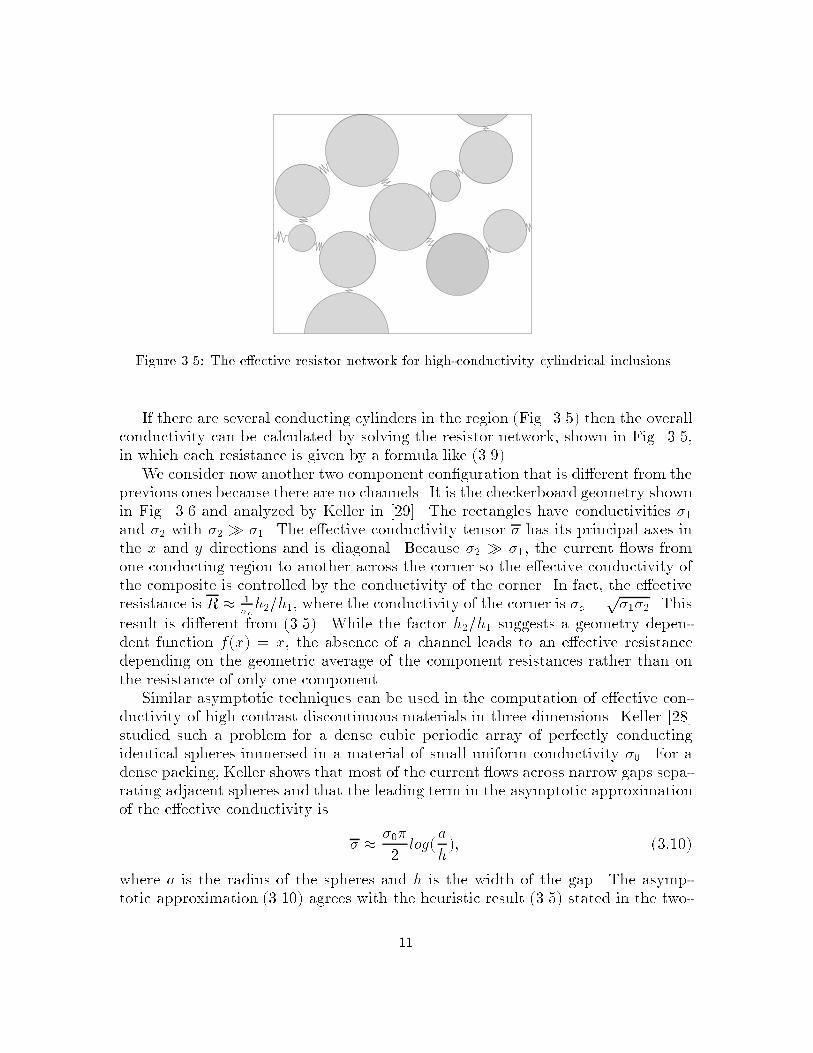
Figure 3.5: The e�ective resistor network for high-conductivity cylindrical inclusions.If there are several conducting cylinders in the region (Fig. 3.5) then the overallconductivity can be calculated by solving the resistor network, shown in Fig. 3.5,in which each resistance is given by a formula like (3.9).We consider now another two component con�guration that is di�erent from theprevious ones because there are no channels. It is the checkerboard geometry shownin Fig. 3.6 and analyzed by Keller in [29]. The rectangles have conductivities �1and �2 with �2 � �1. The e�ective conductivity tensor � has its principal axes inthe x and y directions and is diagonal. Because �2 � �1, the current ows fromone conducting region to another across the corner so the e�ective conductivity ofthe composite is controlled by the conductivity of the corner. In fact, the e�ectiveresistance is R � 1�ch2=h1, where the conductivity of the corner is �c = p�1�2. Thisresult is di�erent from (3.5). While the factor h2=h1 suggests a geometry depen-dent function f(x) = x, the absence of a channel leads to an e�ective resistancedepending on the geometric average of the component resistances rather than onthe resistance of only one component.Similar asymptotic techniques can be used in the computation of e�ective con-ductivity of high contrast discontinuous materials in three dimensions. Keller [28]studied such a problem for a dense cubic periodic array of perfectly conductingidentical spheres immersed in a material of small uniform conductivity �0. For adense packing, Keller shows that most of the current ows across narrow gaps sepa-rating adjacent spheres and that the leading term in the asymptotic approximationof the e�ective conductivity is � � �0�2 log(ah); (3:10)where a is the radius of the spheres and h is the width of the gap. The asymp-totic approximation (3.10) agrees with the heuristic result (3.5) stated in the two-11

xy h1h2�2 � �1�1 �1�2 � �1Figure 3.6: Rectangular checkerboarddimensional case and shows that when the spheres touch each other the e�ectiveconductivity has a logarithmic singularity.We consider next continuous media with logarithmic high contrast properties.3.2 Local Analysis of Static Transport Properties of a High ContrastContinuumWe restrict attention �rst to a purely resistive problem (equations (3.1), (3.2))for a continuous medium with the microscopic resistance �(x) = �0e�S(x)�2 . Thegeometry of the composite is sketched in �gure 3.7. The microscopic resistance �(x)has two minima at xm1 and xm2, two maxima at xM1 and xM2, and a saddle pointxs. At this point the function �(x) is maximum in the x direction and minimum inthe y direction. In a small neighborhood of xs the function S has the approximateexpression S(x) � S(xs) + k�(x � xs)22 � k+(y � ys)22 : (3:11)The geometry we consider here is the continuous equivalent of the discrete case wepresented before and, therefore, we expect the following ow behavior.The e�ective resistance is given by R � �(xs)qk+k� with the ow concentrated inthe driving direction around the saddle point xs .We give a heuristic derivation of this result motivated by the previous examplesand return in x4 to give a proof based on variational principles. Just like the previouscases the current will be small in regions with high resistance and in particular in12

xy1

0 1xsxm1 xm2xM1xM2Figure 3.7: Resistance �(x) with a single saddle point in the domainthe vicinity of the maxima xM1 and xM2. Around the minima xm1 and xm2, thebowl shaped resistance function �(x) will cause the ow to stall. The only way forthe current to pass through the highly resistive region created by the two maximaof �(x) is by concentrating in a small neighborhood of the saddle point xs. Thesmall neighborhood of the saddle-point acts like a bottleneck for the current ow,so it is su�cient to solve the cell problem (3.1) in the vicinity of xs and to look for acurrent in the x direction. The current is given by j = r?u, where u can be viewedas the magnetic �eld in the direction perpendicular to . In order for the currentto be in the x direction, u must be a function of y only. In a small neighborhood ofxs, where S(x) has the expression (3.11), the direct cell problem (3.1) simpli�es toddy [exp(k+(y � ys)22�2 )dudy ] = 0 (3:12)with the normalization conditionZjy�ysj��(�dudy )dy = 1 (3:13)for some � > 0 �xed.Equation (3.12) gives u0(y) = �D � exp(�k+(y�ys)22�2 ), where D is a constant ob-tained from (3.13): Dq 2��2k+ = 1. The solution of the direct problem (3.1) is thenj � 1q 2�k+ �exp(�k+(y � ys)22�2 )e1 (3:14)13

�� C C � � �� CI II IIIL L0x1 x2 x3Figure 3.8: Medium layered acrossthe driving direction xy LI II�� C �� Cx1 x2Figure 3.9: Enlarged view of the in-terface between two layersand by substituting it in (3.2) we obtain the e�ective resistanceR � �(xs)s2�k� � 12��2k+ Z ys+�ys�� exp(k+(y � ys)22�2 � k+(y � ys)2�2 )dy ��(xs)s2�k� � 12��2 k+s2�k+ � = �(xs)sk+k� : (3.15)Since the curvatures k+; k� have dimensions of 1=L2, this result for the e�ectiveresistance of the composite agrees with (3.5) with f(x) = x. In fact the resultobtained here is more typical because the saddle points are just continuous versionsof the channels, gaps or corners occurring in the discontinuous problems.3.3 The E�ective Quasistatic Impedance of a High Contrast ContinuumCase A: Series ConnectionWe consider the direct problem (2.12) with the coe�cients � and C given by(2.21), de�ned over a region with the geometry shown in Fig. 3.8. The domain isdivided in three regions by curves L and L0. In regions I and III the resistancedominates and has the saddle points x1 2 region I and x3 2 region III oriented inthe x direction. In region II the capacitance is dominant and has a saddle point x2oriented in the x direction. We choose this orientation of the saddles for simplicity.However, the results derived in this section apply to more general orientations, aswell. The functions �(x) and C(x) are smooth and periodic and they equal eachother along L and L0. 14

We apply a driving potential di�erence in the x direction and study the owthrough the cell. From (2.12) we see that in each one of the regions of dominantcapacitance or resistance the problem reduces to the one studied in x3:2. Thus, thecurrent ow is concentrated at the saddle points of � and C and is oriented in thedriving direction x. The question that remains is how the three regions connectwith each other. From Fig. 3.8 we see that it is su�cient to study the connectionbetween regions I and II. The connection between regions II and III is similar.Thus, we concentrate attention to the domain shown in Fig. 3.9.From the periodicity in y of the current and the lack of concentration of thevertical ow in both regions I and II we have< j >I=< j >II= e1: (3:16)Thus, in region I, where the resistance is dominant, the problem reduces tor?[�(jR + ijI)] = 0r � jR = r � jI = 0 (3.17)< jR > = e1; < jI >= 0;where jR; jI are the real and imaginary current densities. It is easy to see thatthe imaginary current is zero, and that the problem reduces to the one studied inx3:2. A similar conclusion applies to region II where the capacitive reactance isdominant. Consequently, the ow behavior in regions I and II is exactly the onestudied in section x3:2.In the vicinity of the curve L the function �(x) (C(x)) is continuously decreasing(increasing) with x. Because the ow is driven in the x direction, it must cross thecurve L. The current will be di�use in regions of this neighborhood where � andC are fairly at, and it will concentrate close to the possible common minima of �and C along L. This current concentration is weaker than the one at saddle pointsbecause it occurs only along one direction (i.e. along L). There is no concentrationin the direction perpendicular to the boundary interface and this leads to a lowerorder term in the e�ective impedance. In the asymptotic limit of in�nitely highcontrast the saddle points of � and C will dominate and the contribution of otherfeatures like the minima along L are negligible. This conclusion is supported bynumerical experiments (see x5:2) and it is proved in x4 using variational principles.We should point out that the same kind of features can occur in the purely resistiveproblem and exactly as we concluded above they are negligible in the computationof the e�ective resistance for very high contrast. The validity of this is again givenby variational principles (see x4:1). When the contrast is not very high, featuresother than the saddle points become important in the computation of Z as is seenin [10].Thus, for computing the e�ective impedance we need only consider small neigh-borhoods of the saddle points of �(x) and C(x) in regions I, and II. Near these15

R CFigure 3.10: Equivalent Series Networkpoints we have�(x) � �(x1)exp(k+1 (y � y1)22�2 � k�1 (x� x1)22�2 ); j x� x1 j< � (3:18)C(x) � C(x2)exp(k+2 (y � y2)22�2 � k�2 (x � x2)22�2 ); j x� x2 j< � (3:19)In these small regions we can solve our cell problem by separation of variables,exactly as in x3:2:jR � 1r 2�k+1 �exp(�k+1 (y � y1)22�2 )e1; j x � x1 j< �jR � 1r 2�k+2 �exp(�k+2 (y � y2)22�2 )e1; j x � x2 j< � (3.20)jI � 0:We use the expression (2.16) for the e�ective impedance and obtainZ � �(x1) Z y1+�y1�� Z x1+�x1�� 12��2k+1 exp(�k+1 (y � y1)22�2 � k�1 (x � x1)22�2 )dxdy +iC(x2) Z y2+�y2�� Z x2+�x2�� 12��2k+2 exp(�k+2 (y � y2)22�2 � k�2 (x � x2)22�2 )dxdy (3.21)� �(x1)vuutk+1k�1 + iC(x2)vuutk+2k�2 :This result, together with the observation that the current has the same normalizedaverage over regions I or II as over the entire cell, tells us that our problem is16

�� CC � ��� C IIIIIILL0 x1x2x3Figure 3.11: Medium layered alongthe driving direction xy LIII �� C�� Cx2x1Figure 3.12: Enlarged view of theinterface between two layersasymptotically equivalent to the discrete series circuit shown in Fig. 3.10. We haveonly two network elements: one resistorR = �(x1)rk+1k�1 placed at x1, and a capacitorC = C(x2)rk+2k�2 placed at x2. The current passing through R is < jR + ijI >I= e1,and the current passing through C is < jR + ijI >II= e1.Case B: Parallel ConnectionWe consider the direct problem (2.12) with the coe�cients � and C given by(2.21), de�ned over a region with the geometry shown in Fig. 3.11. The domainis divided in three regions by curves L and L0. In regions I and III the resistancedominates and has the saddle points x1 2 region I and x3 2 region III oriented inthe x direction. In region II the capacitance is dominant and has a saddle point x2oriented in the x direction, as well. The functions �(x) and C(x) are smooth andperiodic and they equal each other along L and L0.We apply a driving potential di�erence in the x direction and study the owthrough the cell. From (2.12) we obtain thatr? � [�(jR + ijI)] = 0 for x 2 region I or III (3.22)r? � [C(jR+ ijI)] = 0 for x 2 region II;where jR and jI are the real and imaginary current densities. The ow is drivenin the x direction so we have < jR + i jI >= Ke1, where K is a complex constant ux. We can rewrite the current densities asjR = real(K)e1 +r?u; jI = imag(K)e1 +r?v;where u and v can be viewed as the real and imaginary parts of the magnetic �eld.17

The functions u(x) and v(x) are periodic in the domain and satisfy the conditions< r?u >=< r?v >= 0:From the periodicity in x of both u and v it follows that in each region there is nonet ux in the y direction. For the ow in the x direction we haveZI j � e1dx + ZII j � e1dx+ ZIII j � e1dx = Ce1 (3:23)which is equivalent to Zi jR � e1dx = �ie1; i = I; II; or IIIZi jI � e1dx = �ie1 (3.24)Xi �i = real(K);Xi �i = imag(K):Equations (3.22) with the driving conditions (3.24) are very similar to the prob-lem studied in x3:2 and give that the ow in each region of the domain is concen-trated at the saddle points of � and C, respectively. The remaining question ishow the regions connect with each other. We notice that the connection betweenregions I and II is similar to the connection between regions II and III. Thus, itis su�cient to study the ow in the domain shown in Fig. 3.12.For simplicity we assume that the average ow over regions I and II isZI jdx+ ZII jdx = e1:A di�erent driving condition with both real and imaginary net uxes does not a�ectthe expression of the e�ective impedance, it just modi�es the uxes of current inthe channels (saddles). Consequently, we haver? � [�(jR + ijI)] = 0< jR > = �1e1< jI > = �1e1 (3.25)r � jR = r � jI = 0x 2 region I;r? � [iC(jR + ijI)] = 0< jR > = �2e1< jI > = �2e1 (3.26)r � jR = r � jI = 0x 2 region II:18

In the vicinity of the curve L the function �(x) (C(x)) is continuously decreasing(increasing) with y. In this region the current is di�use and small where � and Care fairly at. If for example � and C have two maxima along L and a minimumin between, because we have no driving force in the y direction the current avoidsthe two maxima and is relatively small at the minimum as well. Consequently, thebehavior of the ow for this problem is dictated by what happens in regions I, andII, for which we already know the result. This case is a little more complicatedthan case A because the current is divided between the two regions of our domain.Since the average current over the domain shown in Fig. 3.12 is e1, we must have�1 + �2 = 1 (3.27)�1 + �2 = 0:We already know that in order to obtain the e�ective impedance of the regionsI and II it is su�cient to look only in small neighborhoods of saddle points of �and C. In the vicinity of these points we have�(x) � �(x1)exp(k+1 (y � y1)22�2 � k�1 (x � x1)22�2 ); j x� x1 j< �; (3:28)C(x) � C(x2)exp(k+2 (y � y2)22�2 � k�2 (x � x2)22�2 ); j x� x2 j< � (3:29)and by using separation of variables in (3.25) and (3.26) we obtainjR + ijI � �1r 2�k+1 �exp(�k+1 (y � y1)22�2 ) + i �1r 2�k+1 �exp(�k+1 (y � y1)22�2 ); j x� x1 j< �(3.30)jR + ijI � �2r 2�k+2 �exp(�k+2 (y � y2)22�2 ) + i �2r 2�k+2 �exp(�k+2 (y � y2)22�2 ); j x� x2 j< �:We can use these results in the formula for the e�ective impedance (2.16) and,after performing straightforward computations, we obtainZ = [R(�21 � �21)� 2C�2�2] + i[C(�22 � �22) + 2R�1�1]; (3:31)where R � �(x1)rk+1k�1 and C � C(x2)rk+2k�2 . In order to determine the uxes�i; �i; i = 1; 2 we look at the potential di�erence r�(x) which is given byr�(x) = (�+ iC)(jR + ijI): (3:32)We multiply equation (3.32) by e1 and average over the domain to obtain< r� � e1 >= �U =< (�+ iC)(jR + ijI) � e1 >= Z: (3:33)19

We can do the same thing for regions I and II. Because r� is periodic over the celland regions I and II have the same boundaries as the cell in the x direction, theaverage potential di�erence for the entire cell equals the average potential di�erenceover regions I and II. Consequently we have�U = Z = R(�1 + i�1) = iC(�2 + i�2): (3:34)Relations (3.34) and (3.27) form a linear system of four equations and fourunknowns with solution �1 = C2R2 + C2 ;�1 = RCR2 + C2 ; (3.35)�2 = � RCR2 + C2 ;�2 = R2R2 + C2 :Using (3.35) in (3.31) we obtain the following expression for the e�ective impedanceZ = RC2R2 + C2 + i R2CR2 +C2 = ( 1R + 1iC )�1: (3:36)This result suggests that the continuous problem is asymptotically equivalent to thediscrete network shown in Fig. 3.13, where a resistor R placed at x1 is connectedin parallel with a capacitor C placed at x2. The current passing through R is< jR+ ijI >I= �1e1+ i�1e1, and the current passing through C is < jR+ ijI >II=�2e1 + i�2e1.4 High Contrast Analysis Based on Variational PrinciplesIn this section we prove that in the asymptotic limit of in�nitely high contrastthe computation of the e�ective impedance can be reduced to the solution of anequivalent network of resistors and capacitors. The e�ective impedance is given byZ =< (�+ iC)j � j > (4:1)where �(x) = �0e�S(x)�2 , C(x) = C0e�P (x)�2 and j is the complex current density whichsatis�es r?[(�+ iC)j] = 0r � j = 0 (4.2)< j >= e1;20

RCFigure 3.13: Equivalent Parallel Networkover the periodic cell . The e�ective impedance can also be obtained from varia-tional principles of saddle point type (2.19) and (2.20). The proofs presented in thissection assume a logarithmic high contrast of the coe�cients � and C, as �! 0.4.1 The High Contrast Approximation in the Static Case with OneChannelWe return to the problem considered in x3:2 in the static, purely resistive circuit,with �(x) = �0e�S(x)�2 . The function S(x) is smooth and periodic. The geometryof the composite is sketched in �gure 3.7. The resistance �(x) has two minima atxm1 and xm2, two maxima at xM1 and xM2, and a saddle point xs. Near the saddlepoint we have S(x) � S(xs) + k�(x � xs)22 � k+(y � ys)22 : (4:3)Under these assumptions we state the following theorem:Theorem 1. The e�ective resistance is given byR � �(xs)sk+k� ; (4:4)with the ow in the driving direction and concentrated around the saddle point xs.The proof of this theorem is based on the variational principles and it was �rstgiven by Kozlov [34]. We de�ne the direct cell problemr? � (�j) = 0< j > = e1 (4.5)r � j = 021

with the associated e�ective resistanceR =< �j � j >; (4:6)and the dual cell problem r � (1�r�) = 0< r� > = e1 (4.7)with the e�ective conductivity � =< 1�r� � r� > : (4:8)The e�ective parameters R, and � can also be obtained from the Dirichlet-typevariational principles R = min<r?u>=e1 < �r?u � r?u >; (4:9)� = min<r�>=e1 < 1�r� � r� > (4:10)since the Euler equations associated with them are exactly (4.5), and (4.7). Notethat in (4.9) we replaced the current density by j = r?u, where u is the magnitudeof the magnetic �eld which is perpendicular to the plane of . We begin with alemma which is proved in [27], pp. 199-200.Lemma 1. The e�ective parameters R and � satisfy the relation R = ��1.In order to prove Theorem 1, we will obtain an upper bound for R from (4.9)which we will match with a lower bound for R obtained from the dual variationalprinciple (4.10).If we select from the eligible �elds r?u in (4.9), those which are nonzero onlyin a neighborhood of xs, we obtain the inequalityR <� min<r?u>�=e1 Zjx�xsj�� � j r?u j2 dx; (4:11)where < r?u >� is the average of r?u in the � - neighborhood of the saddlepoint. From all the possible �elds r?u in (4.11) we choose those which have thecomponent in the direction e2 equal to zero, so that u = u(y) only, and thereforewe obtainR <� Z xs+�xs�� �(xs)exp(�k�(x� xs)22�2 )dx Z ys+�ys�� exp(k+(y � ys)22�2 )(dudy )2dy; (4:12)where R ys+�ys�� (�dudy )dy = 1. We point out that the inequalities above are only asymp-totic and depend on the parameter � which is �xed as � ! 0. More precisely,22

R <� F �;� means R � F �;�(1 + o(1)) with the small order one term tending to zeroas �! 0 with � > 0 �xed. After doing the x integration, (4.12) becomesR <� �(xs)s2�k� �minu Z ys+�ys�� exp(k+(y � ys)22�2 )(dudy )2dy: (4:13)We choose u in (4.13) to minimize the right side. Then u satis�es the Eulerequation ddy [exp(k+(y � ys)22�2 )dudy ] = 0Z ys+�ys�� (�dudy )dy = 1: (4.14)Equations (4.14) are exactly the same as (3.12) and u is given by (3.14), whichsubstituted in (4.13) gives the upper boundR <� �(xs)s2�k� � 12��2k+ Z ys+�ys�� exp(k+(y � ys)22�2 � k+(y � ys)2�2 )dy =�(xs)s2�k� � 12��2k+s2�k+ � = �(xs)sk+k� ; (4.15)This bound is gotten under the hypothesis that the currentr?u is concentratedaround xs, and ows in the driving direction. To obtain a lower bound for R we usethe dual formulation with the variational principle (4.10) and Lemma 1. In (4.10)we select �eldsr� which are concentrated around xs and have nonzero componentsonly in the e1 direction. The minimum over such �elds can only give a larger valueof the functional in (4.10) and we obtain� <� min� Z xs+�xs�� ��1(xs)exp(k�(x � xs)22�2 )(d�dx )2dx Z ys+�ys�� exp(�k+(y � ys)22�2 )dy;(4:16)where R xs+�xs�� (d�dx )dx = 1: The computation for the minimum in (4.16) is exactly thesame as the one for the direct problem. By solving the Euler equation associatedwith (4.16) we obtain d�dx = 1q 2�k� �exp(�k�(x � xs)22�2 ) (4:17)and hence� <� ��1(xs)s2�k+ � 12�k� �2 Z xs+�xs�� exp(k�(x � xs)22�2 � k�(x � xs)2�2 )dx =��1(xs)s2�k+ � 12�k� �2s2�k� �: (4.18)23

Using Lemma 1 and (4.18) we see that R satis�es� = R�1 <� ��1(xs)sk�k+ : (4:19)Combining (4.15), and (4.19) we get the asymptotic behavior of the e�ective resis-tance R � �(xs)sk+k� : (4:20)Since we used a current r?u in the e1 direction and concentrated around xs toget (4.20), Theorem 1 is proved.4.2 High Contrast Approximation in the Static Case with Many Chan-nelsWe shall now describe how to analyze (3.1)-(3.2) and (3.3)-(3.4) when �(x) hasseveral, say M � 2, saddle points in .With each saddle point we associate an e�ective resistance Rj; j = 1; 2; . . . ;Mgiven by the right side of (4.4). This comes from the local analysis around a saddlepoint that was just carried out in Theorem 1. To �nd the currents owing throughthe saddle points we must specify how the e�ective saddle resistances are connectedto each other. We do this by identifying the network associated with the resistancefunction �(x) as follows.With each minimum of the resistance �(x) we associate a node of a network onthe torus T 2 ( which is the region ). The nodes are connected to adjacent nodesif there is a path between two nodes that goes over a single saddle. This path is abranch or a bond that connects two nodes. To avoid complicated terminology andnotation we will assume that the network that is associated with the resistance is arectangular lattice network as in the �gure 4.1. Recall that the network is periodic.Let the index j 2 N denote the set of nodes and Ijk be the current from node jto node k that is a neighbor of j, k 2 Nj. Then Ijk = �Ikj andXk2Nj Ijk = 0; j 2 N (4:21)which is the discrete analog of r � j = 0, Kircho�'s current law for circuits whenthere are no sources or sinks of current in the network. We denote the resistanceof the (j; k) bond by Rjk ( and note that Rkj = Rjk ).With the above notation and Theorem 1 we now conclude that in the multi-saddle case the e�ective resistance (4.9) is bounded from above byR <� 12 Xj2N Xk2NjRjkI2jk (4:22)where the factor 1=2 is needed because each bond is counted twice. We now min-imize (4.22) subject to the condition (4.21) and the discrete analog of the driving24

j kj 0k0Figure 4.1: Periodic resistor networkcondition < j >= e. If for example e = e1, the unit vector in the x direction,we add to the currents Ijk satisfying (4.21) a constant current I in the horizontaldirection so that the net current crossing any vertical line in equals one while thenet current crossing any horizontal line is zero. The equation that the minimizingcurrents must satisfy is from (4.22)Xj2N Xk2NjRjkIjk�Ijk = 0 (4:23)for every current perturbation �Ijk that satis�es (4.21) and has no net ow in thehorizontal or vertical direction.The implications of (4.23) are best analyzed by using the dual network which inthe case of a rectangular network has the form shown in Fig. 4.1 with broken lines.We denote by j 0 2 N 0 the collection of dual nodes and by N 0k0 the collection of dualnodes adjacent to the dual node k0. The dual network is, of course, the one that isassociated with the minima of ��1(x), the conductivity of the continuous medium.A distribution of currents �Ijk that satis�es (4.21) and has no net ow in the xor y direction can be written in the form�Ijk = Hk0 �Hj0 (4:24)in terms of a function Hj0 de�ned on the dual network. Here (j; k) and (j 0; k0) arerelated to each other, as is shown in the �gure, and the relationXk2Nj �Ijk = 025

is equivalent to Xj loop�H = 0which is the sum of H di�erences taken over the dual loop surrounding the node j.We now use (4.24) in (4.23) and note that0 = Xj2N Xk2NjRjkIjk�Ijk = Xj02N 0( Xk02N 0j0(RI)j0k0)Hj0 : (4:25)This basic identity is the analog of integration by parts in the continuum case andsays that the sum over nodes of the network can be replaced by a sum over loops ofthe voltage di�erences (RI) or, what is the same, a sum over the dual nodes. Butin (4.25) the Hj0 are arbitrary since (4.24) must hold for all �Ijk subject to (4.21).Thus, Xk02N 0j0(RI)j0k0 = 0; j 0 2 N 0 (4:26)which is Kircho�'s loop voltage-di�erence law for circuits. Equation (4.26), thecurrent law (4.21) and the driving condition determine uniquely the minimizingcurrents Ijk in the upper bound (4.22).To get the asymptotic equality of the e�ective resistance R of the original prob-lem to the upper bound we just described we must show that the lower bound isthe same as the upper bound. From Theorem 1 and Lemma 1, we know that wehave the bound R�1 <� 12 Xj02N 0 Xk02N 0j0 R�1j0k0V 2j0k0 (4:27)where Rj0k0 is the resistance associated with the dual bond (j 0k0) and equals Rjkfrom formula (4.4) for the saddle is associated with the bond (jk) in the network or(j 0k0) in the dual network (see Fig. 4.1). The potential di�erences Vj0k0 are de�nedon the dual network and satisfy the relation Vj0k0 = �Vk0j0 as well asXk02N 0j0 Vj0k0 = 0; j 0 2 N 0 (4:28)which says that the potential di�erences around a loop (a dual node) vanish. Thedriving condition in (4.27) is that the net potential di�erence across any verticalline must equal one ( driving in the x direction) while the one across any horizontalline is zero.With these conditions on Vj0k0 we can now minimize (4.27) and we �nd, usingthe basic identity (4.25) again, Kircho�'s current law for the minimizing potentialdi�erences Xk2NjR�1jk Vjk = 0; j 2 N: (4:29)But (4.28) and (4.29) are exactly the same equations as (4.21) and (4.26) so, up toscaling by the overall e�ective resistance, it is clear that the upper bound (4.27) is26

the same as the reciprocal of the upper bound (4.22) and this proves the asymptoticform of the e�ective resistance R as the one associated with the resistances (4.4) inthe network formed from the minima (nodes) of the resistance function �(x).4.3 The E�ective Quasistatic Impedance of a High Contrast Contin-uum. Case A: Series ConnectionIn this section we consider the problem de�ned in x3:3 case A. We study the directproblem (2.8) with coe�cients �(x) = �0e�S(x)�2 and C(x) = C0e�P (x)�2 de�ned overa region with the geometry shown in Fig. 3.9. The functions S(x) and P (x)are smooth, �0 and C0 are constants and � is a small parameter. The domain isdivided in two regions by a curve L. In region I the resistance dominates (�� C),in region II C � � and along curve L � = C. We assume that the resistance�(x) has a single saddle x1 in region I and that the capacitance C(x) has a singlesaddle x2 in region II. Both saddles are oriented in the x direction. The currentdensity is divergence free and can be written as j = r?(u+ iv), where u and v arethe real and imaginary parts of the magnetic �eld which is perpendicular on theplane . In x3:3 case A we stated that when we have a driving in the x direction(i.e. < j >= e1), in the asymptotic limit �! 0 we have an equivalent series circuitconsisting of a resistance R placed at the saddle x1 connected with a capacitanceiC placed at the saddle x2. In this section we use the variational principles (2.19)and (2.20) to prove this result.In the vicinity of the saddle points x1 and x2 we havefor x 2 �N(x1) : �(x) � �(x1)exp(�k�1 (x � x1)22�2 + k+1 (y � y1)22�2 ) (4.30)C(x) � 0;for x 2 �N(x2) :�(x) � 0 (4.31)C(x) � C(x2)exp(�k�2 (x � x2)22�2 + k+2 (y � y2)22�2 ):In order to prove the series connection result we have to show that real(Z) = Rand imag(Z) = C. This is done by obtaining matching lower and upper boundsfor the e�ective impedance Z. For example, in order to obtain an upper boundfor real(Z) we choose some particular real current �eld r?u and then performthe maximization over all the eligible imaginary current �elds. From the previous27

results, we have a good clue for what choice of a real current to make. The currentaveraged over the whole domain should be e1, therefore the function v(x; y) isperiodic in the domain, whereas the real current can be rewritten with the help ofa periodic function �(x; y) as r?u = e1 +r?�. We note that our domain has inthe vertical direction the same boundaries as its component regions I and II andwe use the periodicity in y of � and v to show that the currents in the x directionaveraged over regions I or II satisfy1AI ZI(�uy)dxdy = 1AI ZI(1� �y)dxdy = 1; 1AI ZI(�vy)dxdy = 0; (4.32)1AII ZII(�uy)dxdy = 1AII ZII(1� �y)dxdy = 1; 1AII ZII(�vy)dxdy = 0;where AI and AII are the areas of regions I and II. The currents in the y directioncan have di�erent averages as long as they algebraically add to zero. However inthis problem both � and C have a single saddle point in regions I and II. Fromthe results presented in x3:2 and x5:1 we know that all the current is concentratedaround these saddle points. Consider for example x1, where the function � has aminimum in the y direction and a maximum in the x direction. The current willhave x component �uy concentrated around x1, but the y component ux should besmall. The only place where we could have ow in the y direction would be awayfrom the saddle point, where according to Theorem 1 it should be negligible. Thesame conclusion applies to region II.In order to obtain an upper bound on real(Z), we choose the following realcurrent r?u = 8>>>>>>>>>>>>><>>>>>>>>>>>>>: ( 1q 2�k+1 �exp(�k+1 (y�y1)22�2 ); 0) 8x 2 �N(x1)( 1q 2�k+2 �exp(�k+2 (y�y2)22�2 ); 0) 8x 2 �N(x2)0 otherwise (4:33)which is clearly divergence free, and satis�es< r?u >=< r?u >I=< r?u >II= e1; (4:34)where < � > stands for the normalized average over the indicated region. We use(4.33) in the variational principle (2.19) to obtainreal(Z) <� max<r?v>=0 [Z�N(x1) �(x1)e� k�1 (x�x1)22�2 + k+1 (y�y1)22�2 12�k+1 �2 e� 2k+1 (y�y1)22�2 dx�(4.35)2 Z�N(x2)Cdudy vydx� < �(v2x + v2y) >]:28

We take �N(xi) to be the squares j x � xi j< � and j y � yi j< �; i = 1; 2 wherethe small parameter � is �xed, so as � ! 0 we have �� ! 1. The �rst integral in(4.35) isZ�N(x1) �(dudy )2dx � �(x1)2�k+1 �2 Zjx�x1j<� e� k�1 (x�x1)22�2 dx Zjy�y1 j<� e� k+1 (y�y1)22�2 dy �(4.36)�(x1)vuutk+1k�1 = R:Since the maximum over a sum of functionals is less than the sum of the maximawe havereal(Z) <� R+ max<r?v>=0(� < �(v2x + v2y) >) + max<r?v>=0(�2 Z�N(x2)C(x)dudy vydx):(4:37)The trial �eld r?u is zero in the region II n �N(x2) soZ�N(x2)Cdudy vydx = ZII Cdudy vydx = ZII @@y [Cdudy v]dx� ZII v @@y [Cdudy ]dx: (4:38)From the periodicity in y of Cr?uv and equation @@y (C dudy ) = 0 satis�ed by the trial�eld (4.33) we obtain that Z�N(x2) Cdudy vydx � 0: (4:39)We should point out that the argument above is not quite right because thereal current r?u de�ned by (4.33) is discontinuous at the boundaries of �N(x2) soin order to perform the integration by parts in (4.38) we must smooth it out. Weintroduce the cuto� function�2(y) = 8>><>>: 1 for j y � y2 j< �0 for j y � y2 j> � + �where �2(y) decays smoothly to zero over the region � �j y � y2 j� � + �. Wemodify the trial �eld r?u in region II to ber?u = 1r 2�k+2 �e� k+2 (y�y2)22�2 �2(y)e1:This is still consistent with < r?u >II= e1, r � (r?u) = 0 and the periodicity iny of the real current. Since v is also periodic in y we obtain from (4.38)Z�N(x2)Cdudy vydx = � ZII v @@y [Cdudy ]dx �29

(4.40)C(x2)r 2�k+2 � Z��jy�y2 j��+� Zjx�x2j�� e� k�2 (x�x2)22�2 d�2dy v(x; y)dxdy:The function v(�) is bounded and after evaluating the Gaussian integral over x wehave Z�N(x2)Cdudy vydx � C(x2)vuutk+2k�2 Z��jy�y2 j��+� v(x2; y)d�2dy dy: (4:41)By assumption d�2dy is also bounded so from (4.41) we havej Z�N(x2) Cdudy vydx j <� K�; (4:42)where K is a bounded constant. In conclusion, we can make the integral in (4.42)arbitrary small by choosing � small enough, so inequality (4.37) reduces toreal(Z) <� R+ max<r?v>I=0[� ZI � j r?v j2 dx]: (4:43)The Euler equation for the maximum in (4.43) isr? � (�r?v) = 0 8x 2 regionI< r?v >I = 0 (4.44)and has the solution r?v = 0. Thus,real(Z) <� R: (4:45)To get a lower bound on real(Z) we choose in (2.19) the imaginary currentr?v = 0, and thereforereal(Z) � min<r?u>=e1 < � j r?u j2> : (4:46)This is exactly the problem studied in x4:1, so we write directly the result given byTheorem 1 real(Z) >� R: (4:47)The lower bound on real(Z) given by (4.47) matches the upper bound (4.45) soreal(Z) � R = �(x1)rk+1k�1 . This result was obtained with a real current, concen-trated around the critical points x1;x2 and owing in the driving direction e1. Thecurrent averaged over our domain, or over regions I, or II is equal to e1. Theanalysis for the imag(Z) is exactly the same, and we obtainimag(Z) � C = C(x2)vuutk+2k�2 : (4:48)This completes the analysis of the network approximation for the quasistaticcase with one saddle point in the capacitive and resistive region, respectively, in aseries con�guration. 30

4.4 The E�ective Quasistatic Impedance of a High Contrast Contin-uum. Case B: Parallel ConnectionIn this section we consider the problem de�ned in x3:3 case B. We study the directproblem (2.8) with coe�cients �(x) = �0e�S(x)�2 and C(x) = C0e�P (x)�2 de�ned overa region with the geometry shown in Fig. 3.12. The functions S(x) and P (x)are smooth, �0 and C0 are constants and � is a small parameter. The domain isdivided in two regions by a curve L. In region I the resistance dominates (�� C),in region II C � � and along curve L � = C. We assume that the resistance �(x)has a single saddle x1 in region I and that the capacitance C(x) has a single saddlex2 in region II. Both saddles are oriented in the x direction. The current densitycan be written as j = r?(u+ iv), where u and v are the real and imaginary parts ofthe magnetic �eld which is perpendicular on the plane . In x3:3 case B we statedthat when we have a driving in the x direction (i.e. < j >= e1), in the asymptoticlimit �! 0 we have an equivalent parallel circuit consisting of a resistance R placedat the saddle x1 connected with a capacitance iC placed at the saddle x2. In thissection we use the variational principles (2.19) and (2.20) to prove this result.In the vicinity of the saddle points x1 and x2 the coe�cients �(x) and C(x) aregiven byfor x 2 �N(x1) : �(x) � �(x1)exp(�k�1 (x � x1)22�2 + k+1 (y � y1)22�2 ) (4.49)C(x) � 0;for x 2 �N(x2) :�(x) � 0 (4.50)C(x) � C(x2)exp(�k�2 (x � x2)22�2 + k+2 (y � y2)22�2 ):In order to show the parallel connection we must show that Z � ( 1R+ 1iC )�1. Thisis done by getting matching lower and upper bounds on the e�ective impedance Z.In order to obtain an upper bound on real(Z) we choose in the variational principle(2.19) a particular real current r?u and then perform the maximization over theimaginary current. The experience gained from studying the static case suggeststhat the current should be concentrated around the critical points x1 and x2. Thecurrent averaged over the whole domain should be e1, and therefore the functionv which appears in the expression of the imaginary current must be periodic in .The real current can be written as r?u = e1 + r?�, where � is also a periodic31

function in . We notice that the domain shown in Fig. 3.12 has in the horizontaldirection the same boundaries as its component regions I and II. Consequently,the periodicity over x of both �, and v tells us that the average of the currents inthe y direction over each one of the regions will be1AI ZI uxdxdy = 1AI ZI �xdxdy = 0; 1AI ZI vxdxdy = 0;1AII ZII vxdxdy = 1AII ZII �xdxdy = 0; 1AII ZII vxdxdy = 0 (4.51)where AI and AII are the areas of regions I and II. The currents in the x directioncan have di�erent averages which must satisfy< �uy >I + < �uy >II= 1< �vy >I + < �vy >II= 0: (4.52)We choose as a real current trial �eldr?u = 8>>>>>>>>>>><>>>>>>>>>>>: I1( 1q 2�k+1 �exp(�k+1 (y�y1)22�2 ); 0) 8x 2 �N(x1)I2( 1q 2�k+2 �exp(�k+2 (y�y2)22�2 ); 0) 8x 2 �N(x2)0 otherwise (4:53)which is clearly divergence free. The constants Ii; i = 1; 2 are the ux of realcurrent through each saddle and according to (4.52) they must satisfyI1 + I2 = 1: (4:54)Equation (4.54) is Kircho�'s current law coming from the divergence free condi-tion imposed on the real current. We use (4.53) in the variational principle (2.19)and obtainreal(Z) <� minIi max<r?v>=0 [ Z�N(x1) �(x1)e� k�1 (x�x1)22�2 + k+1 (y�y1)22�2 I212�k+1 �2 e� 2k+1 (y�y1)22�2 dx �(4.55)2 < Cr?u � r?v >II � < � j r?v j2>]:The neighborhoods of x1 and x2 are the squares j x�xi j< �; j y�yi j< �; i = 1; 2where the small parameter � is �xed, so as � ! 0 we have �� !1. The �rst termin (4.55) is a Gaussian integral which givesZ�N(x1) � j r?u j2 dx � I212�k+1 �2�(x1) Z�N(x1) exp(��k�1 (x� x1)22�2 � k+1 (y � y1)22�2 ) �32

(4.56)I21�(x1)vuutk+1k�1 = RI21 :From (4.51) and (4.52) we know that the imaginary current in the x direction(r?v � e1 = �vy) satis�es < �vy >I + < �vy >II= 0whereas the current in the y direction (r?v � e2 = vx) averages to zero in bothregions I and II. We introduce the constants J1 and J2 which are the uxes ofimaginary current in each region, < �vy >I= J1 and < �vy >II= J2. The averagecurrents must satisfy J1 + J2 = 0; (4:57)which is Kircho�'s current law coming from the divergence free condition imposedon r?v.In order to evaluate the integral over �N(x2) in (4.55) we focus on the currentin region II and observe that we can rewrite it asr?v = J2e1 +r? (4:58)where is periodic in region II. We also know that < r?u >= I2e1 orr?u = I2e1 +r?� (4:59)where � is periodic in region II. From (4.58) and (4.59) we haveZ�N(x2)Cr?u � r?vdx = J2 Z�N(x2)Cr?u � e1dx + Z�N(x2)Cr?u � r? dx =J2I2 Z�N(x2)Cr?u � (I2e1 +r?�)dx+ Z�N(x2)Cr?u � r?( � J2I2 �)dx =(4.60)J2I2 Z�N(x2)C j r?u j2 dx+ Z�N(x2)Cr?u � r?( � J2I2�)dx:We use the de�nition (4.53) of the real current and obtain after simple computationsZ�N(x2)Cr?u � r?vdx � J2I2C(x2)vuutk+2k�2 I22 + Z�N(x2)Cdudy @@y ( � J2I2�)dx: (4:61)Since � J2I2� is periodic in region II, the last integral in (4.61) is similar to(4.39) which was studied in x4:3 and shown to be negligible. We use the notationC = C(x2)rk+2k�2 and from (4.55), (4.56) and (4.61) we havereal(Z) <� minIi maxJi [RI21 � 2CI2J2 � min<r?v>=J1e1 < � j r?v j2>I ]: (4:62)33

The minimization over region I is similar to the static problem considered in x4:1,therefore min<r?v>=J1e1 < � j r?v j2>I� RJ21 : (4:63)Thus, the upper bound on the real part of the e�ective impedance isreal(Z) <� minIi maxJi [RI21 � 2CI2J2 �RJ21 ]; (4:64)where the currents Ii and Ji; i = 1; 2 satisfy Kircho�'s current laws (4.54) and(4.57), respectively.In order to obtain a lower bound on real(Z) we choose an imaginary current�eld r?v = 8>>>>>>>>>>><>>>>>>>>>>>: J1( 1q 2�k+1 �exp(�k+1 (y�y1)22�2 ); 0) 8x 2 �N(x1)J2( 1q 2�k+2 �exp(�k+2 (y�y2)22�2 ); 0) 8x 2 �N(x2)0 otherwise (4:65)which satis�es the divergence free condition and averages to zero (< r?v >= 0).We substitute (4.65) in the variational principle (2.19) and after performing similarcomputations we get a lower bound on real(Z) which matches the upper bound(4.64). Consequently,real(Z) � minIi maxJi [RI21 � 2CI2J2 �RJ21 ]: (4:66)A similar analysis applied to the imaginary part of Z (i.e. variational principle(2.20)) leads to the same currents Ii and Ji; i = 1; 2 and the discrete variationalformulation imag(Z) � minIi maxJi [CI21 + 2RI1J1 � CJ21 ]: (4:67)The equations that the currents must therefore satisfy are8><>: RI1�I1 � CJ2�I2 = 0CI2�J2 +RJ1�J1 = 0 (4:68)where the perturbation currents �Ii and �Ji; i = 1; 2 are arbitrary but must satisfyKircho�'s current laws 8><>: �I1 + �I2 = 0�J1 + �J2 = 0: (4:69)From (4.68) and 4.69) we obtain8><>: RI1 = �CJ2CI2 = RJ1; (4:70)34

which are Kircho�'s loop voltage-di�erence law (discrete version of condition r �[(�+iC)j] = 0). From (4.70) and the driving conditions (4.54) and (4.57) we obtainthe currents I1 = C2R2 + C2 ;J1 = RCR2 + C2 ; (4.71)I2 = R2R2 + C2 ;J2 = � RCR2 +C2 :Substituting these in the variational principles (4.66) and (4.67) we obtainZ � ( 1R + 1iC )�1 (4:72)which is the e�ective impedance of the parallel network.This completes the analysis of the network approximation for the quasistaticcase with one saddle point in the capacitive and resistive region, respectively, in aparallel con�guration.4.5 High Contrast Approximation in the Quasistatic Case with ManyChannelsm

m

mm

m

mS

S

S S

M

MM

SM

S

M

M MFigure 4.2: Critical points of �(x)M

S

S

M

M

m

m

S

S

M

M

S

M

m

m

m

mFigure 4.3: Critical points of C(x)35

The series and parallel resistor-capacitor networks discussed so far are very simpleand their connection is evident. In this section we consider more general resistor-capacitor network approximations and show how to connect the resistive and thecapacitive subnetworks in the domain. We recall that periodicity of the boundaryvalue problem is not necessary for the applicability of the network approximation.We have used periodicity throughout the paper to simplify the analysis, which isvalid for general, nonperiodic structures and arbitrary boundary conditions.�� C �� CLFigure 4.4: Resistor network

�� C �� CLFigure 4.5: Capacitor networkWe explain the way the networks are connected by considering a high contrastmedium with one region with dominant resistance separated from a region withdominant capacitance by an interface L along which � equals C. The current owmay arise from any kind of boundary conditions; the results of this section holdin general. To �x ideas we assume that we have a point current source along theleft boundary and a point current sink along the right boundary, as shown in Figs4.4,4.5. Everywhere else we impose homogeneous Neumann boundary conditions.We assume that �(x) and C(x) have the critical points (maxima, minima andsaddles) shown in �gures 4.2 and 4.3 with symbols M, m, and S, respectively. Con-sider �rst the resistive and capacitive structures separately, ignoring the interfaceL that identi�es the dominant one. Transport in a high contrast material withresistance � that has critical points as shown in Fig. 4.2 is approximated by thatof a resistor network with nodes at the minima of � and branches passing throughthe saddle points of � (see Fig. 4.4). The connection of the current source and sinkto the network dependents on their position relative to the basins of attraction ofthe minima of the resistance (nodes in the network) that are closest to the bound-ary. For the example we are considering the connection is shown in Fig. 4.4. Thecapacitor network approximation is obtained in a similar way and is shown in Fig.4.5.Now we return to the full quasistatic resistive-capacitive medium and cut the36

Figure 4.6: Equivalent resistor-capacitor networkapproximating resistor and capacitor networks with the dividing interface L, asshown in �gures 4.4 and 4.5. Note that since the ow concentrates only at saddlepoints of � or C (resistors or capacitors in the approximating circuit) and mergesin the vicinity of the minima of � or C (nodes in the network), if there is any ow concentration across the interface L then the region around it must be inthe basin of attraction of a node (minimum) in the resistor network and a node(minimum) in the capacitor network. Thus, both � and C must have a minimumalong the interface L, in that region. However, � equals C along L so the nodesin the resistive and capacitive networks that have the minimum on L within theirbasin of attraction are connected to each other. This means that we cannot havean arbitrary arrangement of resistive and capacitive nodes on opposite sides of theinterface L; they must be con�gured compatibly.The high-contrast resistor-capacitor network is, therefore, determined as follows.We cut the resistor and capacitor networks along L, as shown in Fig. 4.4 and 4.5,and identify regions of ow-merging (around minima of � and C) on either side ofit. We also identify the resistive and capacitive nodes (minima) that correspond tothem and connect the loose branches in the resistive region that end in the resistivenodes with the loose branches in the capacitive region that end in the adjacentcapacitive nodes. The connection for the example considered is shown in Fig. 4.6.The construction of the resistor-capacitor network for high contrast media gen-eralizes to an arbitrary number of regions with dominant resistive and capacitiveproperties. However, special, nongeneric con�gurations need additional considera-tions. For example, when critical points of � and C are on the dividing interface L,a special situation, a more detailed analysis is needed.37

02

46

8

0

2

4

6

80

1

2

3

4

5

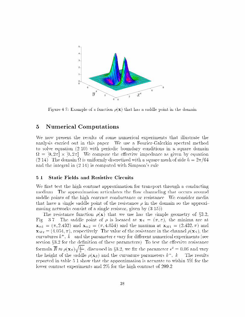
xyFigure 4.7: Example of a function �(x) that has a saddle point in the domain5 Numerical ComputationsWe now present the results of some numerical experiments that illustrate theanalysis carried out in this paper. We use a Fourier-Galerkin spectral methodto solve equation (2.10) with periodic boundary conditions in a square domain = [0; 2�] � [0; 2�]. We compute the e�ective impedance as given by equation(2.14). The domain is uniformly discretized with a square mesh of side h = 2�=64and the integral in (2.14) is computed with Simpson's rule.5.1 Static Fields and Resistive CircuitsWe �rst test the high contrast approximation for transport through a conductingmedium. The approximation articulates the ow channeling that occurs aroundsaddle points of the high contrast conductance or resistance. We consider mediathat have a single saddle point of the resistance � in the domain so the approxi-mating networks consist of a single resistor, given by (3.15)).The resistance function �(x) that we use has the simple geometry of x3:2,Fig. 3.7. The saddle point of � is located at xS = (�; �), the minima are atxm1 = (�; 2:432) and xm2 = (�; 4:054) and the maxima at xM1 = (2:432; �) andxM2 = (4:054; �), respectively. The value of the resistance in the channel �(xS), thecurvatures k+; k� and the parameter � vary for di�erent numerical experiments (seesection x3:2 for the de�nition of these parameters). To test the e�ective resistanceformula R � �(xS)qk+k� , discussed in x3:2, we �x the parameter �2 = 0:06 and varythe height of the saddle �(xS) and the curvature parameters k+; k�. The resultsreported in table 5.1 show that the approximation is accurate to within 5% for thelower contrast experiments and 2% for the high contrast of 209:2.38

0 1 2 3 4 5 60

1

2

3

4

5

6 xsxy Figure 4.8: Flow concentrated atthe saddle point of the resistance fora contrast max(�)=min(�) = 209:2 0 1 2 3 4 5 60

1

2

3

4

5

6 xsxy Figure 4.9: Flow is spread out andnot concentrated at the saddle pointof the resistance for a contrast of �lowered to 9.1�(xs) k+ k� Contrast R Rnum Rel. error (%)1. 1.4 1.8 70.1 1.1339 1.2011 5.394.1727 2.6 3.4 89.3 3.6489 3.4714 -4.862.0427 0.8 2. 97.1 1.2919 1.3478 4.334.1727 2.4 1.6 209.2 5.1105 5.2114 1.97Table 5.1: Dependence of R on the resistance and curvatures at the saddle pointThe accuracy of the resistor approximation is expected to depend on the contrastmax(�)=min(�), so we test it further by �xing the curvatures k+ = 2:4 and k� = 1:6and varying �. The results reported in table 5.2 show that for contrast of order (102)the error is small but the approximation is quite inaccurate for lower contrasts. Aswe show in Fig. 4.8, for a su�ciently high contrast of the ow is channeled at thesaddle point of � and the asymptotic analysis holds. However, when the contrastis low (see Fig. 4.9), the current ow is spread out throughout the domain and theresistor approximation is inaccurate.5.2 Quasistatic Fields and Resistor-Capacitor CircuitsWe now test the high contrast approximation by discrete resistor-capacitor networksfor quasistatic ows.Case A: Series connection 39

Contrast �(xs) �2 R Rnum Rel. error (%)9.1 1.1331 0.8 1.3878 1.1744 15.3852.6 1.1814 0.6 1.4469 1.3281 -8.2165.3 1.3956 0.3 1.7093 1.8176 6.34165 2.7183 0.1 3.3292 3.4212 2.46209.2 4.1727 0.06 5.1105 5.2114 1.97Table 5.2: Accuracy of the resistor network approximation versus the contrast0 1 2 3 4 5 6

0

1

2

3

4

5

6

x

y

7.82

7.82

4.47

3.35

2.24

4.47 2.24

1.12

1.12

2.24

1.12

2.24

1.12

1.12Figure 5.1: Microscopic resistance�(x) 0 1 2 3 4 5 60

1

2

3

4

5

6

x

y

1.12

1.12

2.23

2.23

1.12

7.81

5.58

3.35

2.23

7.81

4.47 3.35 2.23 5.58Figure 5.2: Microscopic capacitanceC(x)To test the range of validity of the resistor-capacitor series network approxima-tion we consider functions �(x) and C(x) with geometry similar to the one in x3:3Case A. In Fig. 5.1 and 5.2 we show an example of functions �(x) and C(x) usedin this section. The resistive and capacitive regions are separated by the interfaceat x = � along which � = C. The location of the saddle points, the curvatures ofthe scaled logarithms of � and C at the saddles and the contrast are varied di�er-ent numerical experiments. As discussed in x3:3 Case A, we can have, in additionto the saddle points, regions of weak ow concentration that are negligible in thecomputation of the e�ective impedance in the limit of in�nitely high contrast. Anexample of such a region is the common minimum � = (�; �) of � and C along thedividing interface at x = �.In order to test the accuracy of the resistor-capacitor series network approxima-tion for di�erent contrasts we �x the curvature parameters (see (3.18) and (3.19))k+1 = k�1 = k+2 = 1:, k�2 = 1:6 and the location of the saddle points x1 = (�=3; �)and x2 = (5�=3; �), respectively. The contrast of � and C is changed by varyingthe parameter �. The results of this set of experiments are reported in table 5.3. Asexpected, the approximation is accurate to within a few percent when the contrastis O(102) or higher and quite inaccurate for lower contrasts. The ow correspondingto the �rst entry in table 5.3 is shown in Fig. 5.3. We only show the real part ofthe current ow. The imaginary part is four orders of magnitude smaller than the40

0 1 2 3 4 5 60

1

2

3

4

5

6 �x1 x2xyFigure 5.3: Real current ow for a contrast of � and C of 1015.7�(x1) C(x2) Contrast �2 R Rnum Rel. C Cnum Rel.Error Error28.0316 28.0316 1015.7 0.06 28.0316 29.0506 3.64 % 22.1609 22.2818 0.6 %17.4117 17.4117 978.4 0.07 17.4117 18.0364 3.59 13.7652 13.8814 0.8412.1825 12.1825 853.7 0.08 12.1825 12.6136 3.54 9.631 9.8037 1.735.2945 5.2945 113.4 0.12 5.2945 5.0600 -4.43 4.1857 4.0979 -2.102.7183 2.7183 37.9 0.2 2.7183 2.3028 -15. 2.1490 1.9925 -7.281.9477 1.9477 9.45 0.3 1.9477 1.5001 -23. 1.5398 1.3472 -12.5Table 5.3: Accuracy of the R-C series network approximation versus the contrastreal part, as predicted by the asymptotic theory in x3:2 Case A. We note the strong ow concentration around the saddle points of � and C and the concentration atthe minimum � along the interface separating the resistive from the capacitive re-gion. However, around � the magnitude of the current increases only along the ydirection. Across the interface (x direction), the potential gradient is negligible sowe only have weak ow concentration at �. Thus, in the circuit approximation, thecontribution of this region is equivalent to having a connecting wire of negligibleimpedance.The resistor-capacitor series network approximation was also tested for di�erentlocations and orientations of the saddle points in the resistive and capacitive regions.The results are not in uenced much, as expected, because location and orientationof the saddles does not a�ect the network.41

0 1 2 3 4 5 60

1

2

3

4

5

6

x

y

2

2

14 6

4

2 2 4

4 14

8 6Figure 5.4: Microscopic resistance�(x) 0 1 2 3 4 5 6

0

1

2

3

4

5

6

x

y 2

2 4

2

4 2

4 18

18 8

6

Figure 5.5: Microscopic capacitanceC(x)real imag�(x1) C(x2) �2 real(Z) (Znum) Rel. imag(Z) (Znum) Rel.Error Error12.1825 12.1825 0.08 7.4961 7.3967 -0.82 % 5.9256 5.8333 -1.56 %7.3891 7.3891 0.1 4.5471 4.1970 -7.7 3.6955 4.1172 11.413.7937 3.7937 0.15 2.3346 1.8712 -19.85 1.8457 1.1394 -27.432.7183 2.7183 0.2 1.6728 0.8918 -46.7 1.3225 0.8442 -36.17Table 5.4: Accuracy of the R-C parallel network for di�erent contrasts of � and CCase B: Parallel connectionIn the quasistatic regime we now explore the high contrast approximation witha parallel resistor-capacitor networks. The geometry of the microscopic resistanceand capacitance is similar to the one in x3:3 Case B. In Fig. 5.4 and 5.5 we showan example of functions �(x) and C(x) used in this section. The resistive andcapacitive regions are separated by the interface y = � along which � and C havea common minimum at � = (�; �).We test the accuracy of the network approximation for di�erent contrasts of� and C in a set of experiments with the location of the saddle points kept atx1 = (�; �=3) and x2 = (�; 5�=3) and with the curvature parameters �xed atk+1 = k�1 = k�2 = 1: and k+2 = 1:6. The contrast is varied by changing the parameter�. In tables 5.4 and 5.5 we show the error in the e�ective impedance and thetheoretical and numerically computed current uxes through the channels at thesaddle points of � and C (�i; �i; i = 1; 2 are de�ned in x3:3 case B). The results showthat the parallel resistor-capacitor network approximation is accurate to within few42

0 1 2 3 4 5 60

1

2

3

4

5

6

xy x1x2Figure 5.6: Real current ow for a contrast of � and C of 853.7Contrast �1 �num1 �1 �num1 �2 �num2 �2 �num2853.7 0.6154 0.6120 0.4865 0.4783 0.3846 0.3880 -0.4865 -0.4783140.8 0.6154 0.6013 0.4865 0.4592 0.3846 0.3987 -0.4865 - 0.459289.4 0.6154 0.5534 0.4865 0.3621 0.3846 0.4466 -0.4865 -0.362137.9 0.6154 0.509 0.4865 0.2132 0.3846 0.4910 -0.4865 -0.2132Table 5.5: Real and imaginary current uxes through the channels developed at the saddlepoints of � and Cpercent when the contrast of � and C is O(102) or higher. For lower contrasts, theapproximation is not inaccurate. The real part of the current ow computed withcontrast of � and C equal to 853.7 is shown in Fig. 5.6 . The imaginary part of thecurrent behaves similarly except that while in the resistive channel the ow is in thepositive direction of the x axis, in the capacitive channel the ow is in the oppositedirection. This behavior is, of course, due to the zero imaginary part of the drivingcondition assumed in the computations. The behavior of the current ow con�rmsthe results of the asymptotic theory that is, that the ow concentrates only in thechannels that form at saddle points of the microscopic resistance and capacitance.6 Summary and ConclusionsWe have shown both analytically and numerically that the e�ective resistance andcapacitance of a high contrast material can in certain cases be approximated wellby a resistor-capacitor (R-C) network. In both the static case, where the network43

consists only of resistors, as well as in the quasistatic case, this can be done ingeneral for any number of saddle points of the resistance and capacitance functions�(x), C(x), around which the current concentrates. Variational principles playan essential role in the analysis. We have restricted attention to two dimensionalproblems but the results are general and extend easily to any number of dimensions.Network approximations do not seem to be appropriate for quasistatic resistive-inductive problems because we do not have ow concentration around saddles.There are variational principles for these problems but we do not know how to usethem yet.In [10] we have used the local analysis of the ow around the saddles to constructa very e�cient and accurate hybrid, analytical-numerical method for solving highcontrast conductivity problems. In [8] we have used the static asymptotic theoryto image high contrast media with impedance tomography.AcknowledgementsThis work was partially supported by a grant from AFOSR, F49620-94-1-0436 andby the NSF, DMS 9308471. We thank J. Berryman for many fruitful discussionsand advice on this problem.References[1] Alumbaugh, D. L., 1993, Iterative Electromagnetic Born Inversion Applied toEarth Conductivity Imaging, Ph.D. thesis, Berkeley.[2] Alumbaugh, D.L., Morrison, H. F., 1993, Electromagnetic conductivity imag-ing with an iterative Born inversion, IEEE Transactions on Geosciences andRemote Sensing, Vol. 31, No. 4, pp. 758-763.[3] Ambegaokar, V., Halperin, B. I., Langer, J. S., 1971, Hopping Conductivity inDisordered Systems, Phys. Rev. B, 4(8), pp 2612-2620.[4] Batchelor, G. K., O'Brien, R. W., 1977, Thermal or electrical conductionthrough a granular material, Proc. R. Soc. London A, 355, pp 313-333.[5] Bensoussan, A., Lions, J. L., Papanicolaou, G. C., 1978, Asymptotic analysisfor periodic structures, North-Holland, Amsterdam.[6] Berlyand, L., Golden, K., 1994, Exact result for the e�ective conductivity of acontinuum percolation model, Physical Review B (Condensed Matter), vol.50,no.4, pp 2114-17.[7] Borcea, L., 1996, Direct and Inverse Problems for Transport in High ContrastMedia, Ph.D. thesis, Stanford University.44

[8] Borcea, L., Berryman, J. G., Papanicolaou, G. C., 1996, High ContrastImpedance Tomography, Inverse Problems, 12, pp 1-24.[9] Borcea, L., Papanicolaou, G. C, Wehr, J., Network approximation for highcontrast random conductivities, in preparation.[10] Borcea, L., Papanicolaou G. C., A Hybrid Numerical Method for High ContrastConductivity Problems, to appear in J. Computational and Applied Mathemat-ics, 1996.[11] Cherkaev, A. V., Gibiansky, L. V., 1994, Variational principles for complexconductivity, viscoelasticity, and similar problems in media with complex mod-uli, J. Math. Phys., 35 (1), pp 127-145.[12] Clerc, J.P., Giraud, G., Laugier, J.M. and Luck, J.M., 1990, The electrical con-ductivity of binary disordered systems, percolation clusters, fractals and relatedmodels, Advances in Physics, 39 (3), pp 191-309.[13] Dagan, G., 1989, Flow and Transport in Porous Formations, Springer- Verlag,New York.[14] Dykhne, A. M., 1971,Conductivity of a two-dimensional two-phase system,JETP 32, pp 63-65.[15] Ekeland, I., Teman, R., 1976, Convex analysis and variational problems, Stud-ies in mathematics and its applications, vol. 1.[16] Fannjiang, A., Papanicolaou, G., 1994, Convection enhanced di�usion for pe-riodic ows, SIAM J. Appl. Math., 54, pp 333-408.[17] Fannjiang, A., Papanicolaou, G., 1996, Di�usion in turbulence, ProbabilityTheory and Related Fields, 105, pp 279-334.[18] Fannjiang, A., Papanicolaou, G.C., 1996,Convection enhanced di�usion forrandom ows, to appear in the Journal of Statistical Physics.[19] Gibiansky, L. V., Milton, G. W., 1993, On the e�ective viscoelastic moduli oftwo-phase media. Rigorous bounds on the complex bulk modulus, Proc. R. Soc.London A, 440, pp 163-188.[20] Golden, K.M., Percolation models for porous media, in Homogenization andPorous Media, U. Hornung, ed., Springer Verlag, in press.[21] Golden, K.M., Kozlov, S.M., Critical path analysis of transport in highly dis-ordered random media, preprint 1995.[22] Golden, K., Papanicolaou, G., 1985, Bounds for e�ective parameters of multi-component media by analytic continuation, J. Stat. Phys. 40, pp 655-668.[23] Habashy, T. M., Groom, R. W., Spies, B. R., 1993, Beyond the Born andRytov Approximations: A nonlinear approach to Electromagnetic Scattering,Geophysical Research, Vol. 98, No. B2, pp 1759-1755, February.45

[24] Halperin, B. I., 1989, Remarks on percolation and transport in networks witha wide range of bond strengths, Physica D, 38, pp 179-183.[25] Hashin, Z., Shtrikman, S., 1962, A variational approach to the theory of thee�ective magnetic permeability of multiphase materials, J. Appl. Phys. 33, pp3125-3131.[26] Jackson, J. D., 1974, Classical Electrodynamics, second ed., Wiley, New York.[27] Jikov, V. V., Kozlov, S. M., Oleinik, O. A., 1994, Homogenization of Di�eren-tial Operators and Integral Functional, Springer-Verlag, Berlin Heilderberg.[28] Keller, J. B., 1963, Conductivity of a Medium Containing a Dense Arrayof Perfectly Conducting Spheres or Cylinders or Nonconducting Cylinders, J.Appl. Phys., 34 (4), pp 991-993.[29] Keller, J. B., 1987, E�ective conductivity of periodic composites composed oftwo very unequal conductors, J. Math. Phys., 28 (10), pp 2516-2520.[30] Keller, J. B., 1964, A Theorem on the Conductivity of a Composite Medium,J. Math. Phys., 5(4), pp 548-549.[31] Kitanidis, P. K., 1995, Quasilinear Geostatistical Theory for Inversing, WaterResour. Res., 31, pp 2411-2419.[32] Kohler, W., Papanicolaou, G., 1982, Bounds for the e�ective conductivity ofrandom media, Springer Lecture Notes in Physics 154, pp 111-130.[33] Koplik, J., 1982, Creeping ow in two-dimensional networks, J. Fluid Mech.,Vol. 119, pp 219-247.[34] Kozlov, S. M., 1989Geometric aspects of averaging, Russian Math. Surveys44:2, pp 91-144.[35] Milton, G. W., 1990, On characterizing the set of possible e�ective tensors ofcomposites: The variational method and the translation method, Communica-tions on Pure and Applied Math., Vol XLIII, pp 63-125[36] Schwartz, L. M., Banavar, J. R., Halperin, B. I., 1989, Biased-di�usion calcu-lations of electrical transport in inhomogeneous continuum systems, Physicalreview B, Vol. 40, 13, pp 9155-9161.[37] Shah, C. B., Yortsos, Y. C., 1996, The permeability of strongly-disordered sys-tems, Physics of Fluids, vol.8, no. 1, pp 280-282.46