Neighbourhood Effects and Women’s Health outcomes: A ...

1

Neighbourhood Effects and Women’s Health outcomes: A Multilevel

Perspective

Introduction

Living a healthy long life is at the core of human development and the benefits of a healthy population to any society cannot be over emphasized. Measuring the health-related quality of life within and among population subgroups is crucial in understanding the distribution of health. It helps to focus attention and action on specific health determinants and population groups to reduce inequalities in health and improve health overall. Poor health has both direct productivity losses and large indirect costs to households and the economy (Suhrcke et al., 2006, de-Graft Aikins, 2006, WHO, 2009). Poor health can result in loss of current earnings through absence from work and loss of future earnings because of being unproductive, resulting in one’s inability to meet basic necessities of life. Poor health may also have significant social costs by undermining individual’s autonomy to be self-sufficient (Gaimard, 2014). Adult poor health also has a negative impact on their households and their future. For example, their dependants suffer from lack of care because of the drastic reduction in the household’s income or support, especially when they are the main breadwinners. Such a high morbidity and mortality environment also tends to deter potential investors from investing in such economies (Gaimard, 2014). Research in the field of social epidemiology have argued that beyond the individual characteristics and biological traits, health status of the individual is influenced by the physical, social, geographical environment and changes in their occurrences over time (Balfour and Kaplan, 2002, Do and Finch, 2008, Brown et al., 2007). Studies on the effect of the physical and built environment on a population’s health status have been a recent phenomenon. The literature suggests that place of residence and its environs play an important role in influencing a population’s health status (Stafford and Marmot, 2003, Omariba, 2010, Stronegger et al., 2010). The environment serves as an arena for establishing connections with other individuals, engage in daily activities and developing lifestyle habits (Bernard et al., 2007, Poortinga et al., 2008, Stronegger et al., 2010). With increasing longevity in Ghana, maintaining good health and assessing their health needs of this growing population is a major concern. While the neighbourhood level effects on health status have been described in other research, this is relatively new, especially in Africa. Little work has been done in the West African sub-region to test whether the local environmental factors have any influence on the self-assessed health status of the general population. Very little is known about which neighbourhood characteristics influence either individual’s physical functioning or mental wellbeing. Neighbourhood characteristics such as housing quality, hygienic conditions, socio-economic status can be environments that promote an individual’s positive or negative health experience or help rate their health status in relation to others. One of the commonly discussed ways in which housing influences health status is through human

2

exposure to inadequate housing conditions including overcrowding, and poor ventilation. Housing quality tends to determine the social class and kind of residents living in a particular neighbourhood (Arku et al., 2011, Bonnefoy, 2007, Dunn, 2002, Stronegger et al., 2010). Stronegger and colleagues (2010), for example, observed that, homes and their environment shape an individual’s identity. In Ghana, large single-family detached homes and semi-detached structures in gated neighbourhoods tend to perpetuate occupancy by the high SES groups. Flats and apartment buildings with separate dwelling units and modest amenities tend to perpetuate occupancy by middle-income households, while large compound or shared houses have smaller dwelling units with moderate to insufficient amenities tend to be patronised by households of lower socio-economic status. A study carried out in two neighbourhoods in Vancouver, Canada found that owner-occupiers were significantly more likely to report better health status and mental health status than non-owner occupiers (Dunn, 2002). Arku et al. (2011), replicating the study in three localities in Accra, Ghana, found that overall, women, with low educational levels, living in poor housing conditions and residing in poor localities, assessed their self-rated health as poor. Arku and colleagues (2011) focused on individual housing characteristics and not neighbourhood variables’ effect on self-rated health. This study extend the investigation further by assessing neighbourhood factors and their effect on their overall physical functioning and mental or emotional wellbeing, for all clusters in three districts in the Greater Accra Region. The neighbourhood in which one lives may exert both direct and indirect influence on the health outcome of the residents. Environmental factors may also change people’s susceptibility to disease for example, the availability and affordability of food high in fat and sugars, alcohol, illegal drugs, or hygienic environment, or conflict free communities. Studies have shown that neighbourhoods of residence are endowed with certain resources that may help shape the individual health status and social functioning. (Stronegger et al., 2010, Brown et al., 2007), have reported associations between low socio-economic status neighbourhoods and poor health status among the residents; others have investigated neighbourhood effect on the elderly and various segments of the population. Such associations have been observed for a variety of health outcomes including perceived health (Blaxter, 1990, Do and Finch, 2008, Omariba, 2010). Others suggest that some neighbourhoods are healthier than others are (Brown et al., 2007, Stafford and Marmot, 2003, Poortinga et al., 2008). The World Health Organisation (WHO) defines health status as ‘a state of complete physical, mental and social well-being and not merely the absence of disease and infirmity’ (WHO, 1948: 1). It can be argued that while only few individuals within the population are mentally ill and or physically challenged, mental wellbeing and physical functioning is something that everyone experiences and at varying degrees. There is therefore the need to measure physical functioning or health status and mental wellbeing appropriately among the adult population in order to assess their relationship with individual and neighbourhood characteristics. This paper focuses on the city of Accra, Ghana to better understand what aspects of residents’ perception of their neighbourhood hygienic condition, neighbourhood housing quality and neighbourhood socio-economic status are associated with their physical functioning and mental wellbeing.

3

This paper focuses on a general hypothesis about the overall effect of neighbourhood factors (both direct and indirect) on Physical Health status (PCS) and emotional wellbeing (MCS) separately. Are residents in neighbourhoods with poorer housing quality, a lower hygiene index and lower neighbourhood SES associated with poor PCS and/or MCS score in the same way? Does the association between neighbourhood indices and PCS or MCS persist after adjusting for individual demographic, socio-economic and health-related factors? Researching into how neighbourhood factors might influence a population’s health status, beyond individual characteristics, might offer new understanding and provide effective forms of policy recommendations.

Data and methods

The study draws on the second wave of the 2008 Women Health Study of Accra (WHSA),

conducted by the Institute of Statistical Social and Economic Research (ISSER), University of

Ghana and the Department of Global Health and Population (GHP), Harvard School of Public

Health. The study also extracted contextual information from the 2000 Ghana Population

and Housing Census (GPHC) datasets for the study areas. The 2000 GPHC is a structured

pre-coded protocol consisting of 30 population related questions and 17 housing questions.

Information was gathered at the enumeration areas (EAs). The extracted information from

the 2000 GPHC data was merged with the individual files from the 2008 survey at the PSU

level. Each respondent has a unique code and these codes facilitated the linking of the

various datasets, whilst also ensuring no duplication of cases.

Outcome variables

The outcome variables for this analysis are the two component summary scores: the Physical Health Component Summary (PCS) and the Mental Health Component Summary (MCS) scores. These were derived using varimax rotated factor analysis involving the eight SF-36 sub-scales and classified into quintiles (1-5), retaining their natural ranking order. These were classified as ‘Poor’, ‘Fair’, ‘Good’, ‘Very good’ and ‘Excellent’ separately for PCS and MCS. The SF-361 is a multi-item scale used to assess the health of the general population across eight-health concepts. These include physical functioning (PF), role limitation due to physical health problems (RP), bodily pain (BP), role limitations due to personal or emotional problems (RE), general health perception (GH), social functioning (SF), vitality (VT), and general mental health (MH). In addition, the eight scales yield two summary scores (Physical Component Summary- (PCS) and Mental Component Summary (MCS)) relating to physical functioning and emotional wellbeing (Fukuhara et al., 1998, Ware and Sherbourne, 1992, Ruta et al., 1998). The SF-36 has been designed to satisfy psychometric standards required for group comparisons (Ware et al., 1998, Butterworth and Crosier, 2004, Hays et al., 1993), as well as represent the multidimensional nature of

1 The SF-36 items scale was developed by Ware and Sherbourne (1992) from items originally included in the

Medical Outcomes Study (MOS) long form measures developed for use in the Rand Corporation’s Health Insurance Experiment (Brazier et al, 1992; Jenkinson and McGee, 1998).

4

health (McHorney et al., 1993). These measures tap a broader spectrum of health status and are suitable for assessing group differences.

Explanatory variables

Individual compositional factors and neighbourhood level variables were employed in this study. Neighbourhood variables were computed from the responses to the 2000 GPHC questionnaire. The analysis adopted the boundary classification area into census clusters, which had already been employed in the WHSA surveys. The 2000 GPHC database held several cluster level measures of socio-economic status, hygiene and housing quality indicators. A total of 63 cluster-level variables were extracted and grouped into three sub-categories, namely, cluster socio-economic status, hygiene index and housing quality index. A data reduction strategy, principal component analysis was used to obtain the principal component for each of the indices. Cluster hygiene index, housing quality index and neighbourhood SES index were classified into quintiles and labelled as 1 ’lowest’, 2 ‘low’, 3 ‘average’, 4 ‘higher’ and 5 ‘’highest’ or its equivalent. Since the respondents were also selected from the census cluster areas, the extracted neighbourhood information were merged to the survey data using the unique neighbourhood identification codes.

Control variables

Individual level variables included in the study were taken from the 2008 household survey. The factors included age, education, marital status, parity, ethnicity, wealth status, physical activity, alcohol consumption, social networks and disease symptom, where applicable.

Statistical method

Two methods of analyses were used to examine the level of self -assessed physical functional and emotional wellbeing among the study population and the factors that explain the differentials. The first part of the analysis explores the weighted associations between each of the outcome variables and the selected background and health characteristics, using Pearson’s chi-squared distribution tests. The second segment of the analysis investigates the contextual effect of neighbourhood of residence on the PCS and MCS separately, using multilevel ordinal logistic regression approaches (Rabe-Hesketh and Skrondal, 2008, Snijders and Bosker, 2012, Hilbe, 2009). This technique was adopted to examine the hierarchical structure of the effect of contextual factors on the observed patterns in the levels of self-assessed health status.

Results

Physical Health (PCS) differentials

Test of associations between physical health status by the individual background characteristics revealed that respondents’ age was negatively associated with physical

5

functioning. The results show that there was a steady decline in the overall PCS score as age progresses up to 49 years. The PCS deterioration became dramatic beyond 49 years. Less than 13% of respondents aged 60 years or older rated their health as either ‘very good’ or ‘excellent’ PCS compared to more than 64% among the youngest age group. Education maintained a positive association with the PCS score. Among women with secondary or higher education, less than 8% rated their PCS as ‘poor’, while 28.6% assessed their PCS as ‘excellent’, compared to 34% and 11% respectively among women with ‘no education’. The association between PCS score and marital status showed that women, ‘formerly in union’, nearly 29%, assessed their health as ‘poor’ compared to 11% of ‘currently married’ women, while the ‘never married’ individuals maintained the highest proportion rating their PCS, as excellent. The results further showed that women with higher numbers of children born assessed their health status less favourably across the PCS categories compared to women with few children. The higher the wealth status of the individual, the less likely the respondent assessed her PCS score as ‘poor’. Of women who experienced no disease symptoms, 5%, rated their health status as ‘poor’ and this proportion increased sharply with an additional symptom experienced to 14% and 28% among respondents that experienced ‘single’ and ‘multiple symptoms’, respectively. Lifestyle activities, such as alcohol consumption, did not show much variation in terms of ‘poor’ PCS assessment, but did show significant variation towards an ‘excellent’ PCS score. A greater proportion of respondents who were actively engaged in physical activities, rated their PCS score as ‘excellent’ than respondents who were inactive.

Mental Health (MCS) differentials

Tests of association between the MCS score and selected individual characteristics was roughly bell-shaped. This pattern is slightly different from that observed in total PCS score, where the distribution was slightly negatively skewed, reflecting the presence of better physical health than mental health status. The MCS score’s association with respondents’ age was not as clear-cut, even though the overall association was significant. More than 30% of respondents in the oldest age group rated their mental health as ‘excellent’, while less than 18% recorded this among the younger age groups (20-49). A higher proportion of respondents with primary or no education assessed their MCS score lower than respondents with secondary or higher. Respondents of the poorest households 27% rated their MCS as ‘poor’ decreasing progressively to 14% among the richest households. Among women who had had limited social interactions, or unable to participate in community activities, a higher proportion assessed their health status as ‘poor’ on MCS. Respondents who had experienced ‘multiple’ disease symptoms, a higher proportion rated their mental health status as ‘poor’, decreasing steadily with those who had experienced a ‘single’ symptom and ‘no symptom’ in that order. The association between MCS scores and marital status, parity and ethnic groupings showed irregular patterns. For example, a higher proportion of formerly married women rated their MCS as ‘excellent’. Similarly, a higher proportion of respondents with 5 or more children rated their MCS as ‘excellent’. Alcohol consumption maintained a weak association with overall mental health.

6

Multilevel modelling- two component health scores A random intercept cumulative logit model was fitted for the Physical and Mental health separately. Model I consisted of only the random intercept (neighbourhood level-II). The second model included the individual compositional factors and then, finally, the neighbourhood level variables were included to fit Model III. Control variables that were not significant at the point of inclusion were excluded and the model re-fitted. Model I in the multilevel analysis addressed the research question, examining whether there were between neighbourhood variations in any of the two outcome measures of self-assessed health. Model III addressed the objective of examining the effects of the contextual factors on the two outcome variables, controlling for individual factors. The resulting neighbourhood-level variance estimates were used to compute the variance partition coefficient and the percentage change in variance, explaining the outcome variable of interest. The findings presented in this analysis are based on the final model (Model III), unless otherwise specified.

Factors associated with Physical Health component score

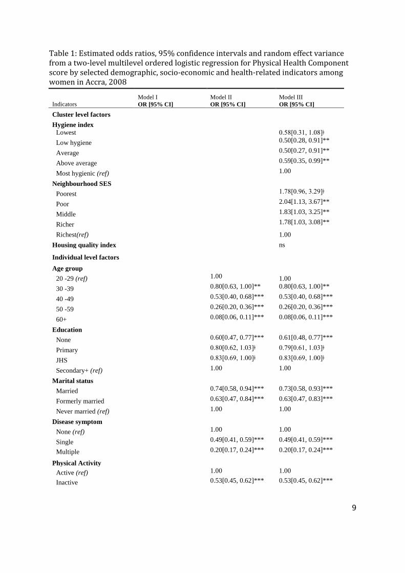
The result from Model I (without any covariates) showed that the estimate of neighbourhood-level variance (0.343, SE 0.063) was significant at p≤0.001. This implies that, without accounting for any predictors in the model, there were significant differences in levels of the PCS score among the various neighbourhoods in Accra, with a variance partition coefficient (VPC) value of 9.4%. Model II, which includes individual compositional factors, yielded a VPC value of 12.2%. Accounting for the three neighbourhood factors (hygiene index, housing quality index and neighbourhood SES) suggests that 10.9% of the variability in physical health status lies between neighbourhoods of residence. The results further revealed that the differences in physical health according to neighbourhood characteristics remained significant even after adjusting for other predictors. This shows that the neighbourhood in which a woman resides significantly influence her physical health status. The results from Table 1 revealed that the association between neighbourhood SES and physical health status was different from expectation. Surprisingly, holding all individual and other contextual factors constant, neighbourhood SES maintained a graded negative association with PCS. The results show that apart from residents found in the ‘poorest SES neighbourhoods’ whose association with PCS could not be statistically substantiated at p<0.05, all other SES neighbourhood categories were significant. The results show that the odds of being in a lower response category for all cut-points (K11-14) on PCS among respondents resident in ‘poor SES neighbourhoods, were 2 times less likely than among resident in the richest SES neighbourhoods, the reference group. Respondents resident in middle SES neighbourhoods were 83% less likely than residents in the richest SES neighbourhoods, the reference group to be in a lower response category on PCS for all cut-points (K11-14), holding all other factors in the model constant. Similarly, respondents

7

resident in richer SES neighbourhoods were 78% less likely, to be in a lower response category on PCS for all cut-points (K11-14) than among residents in the richest SES neighbourhoods, the reference group. There was a particularly large differences between the odds of obtaining a higher score category on PCS among residents in poor neighbourhoods than among the ‘richest’ neighbourhoods, the reference.

Factors associated with Mental Health component score

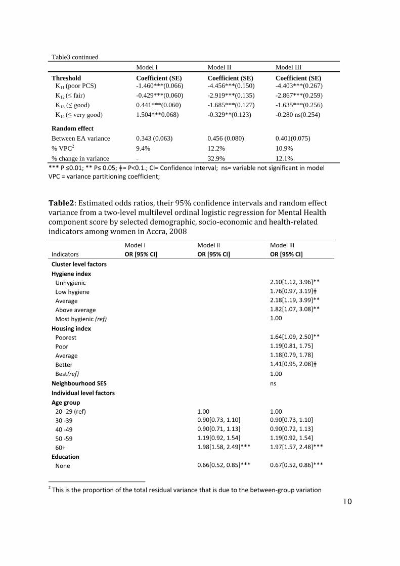
The results also report on the threshold parameter estimates and the estimated variance partition coefficient (neighbourhood level variance) attributable to the unexplained differences in the levels of health status among respondents, after accounting for the factors in the model. The variance partition coefficient measured in Model I shows that 13.7% of the total variation in the propensity to have a higher score for MCS that was due to differences between neighbourhoods. Model II, which consists of the individual compositional factors, the total variance between group differences yielded a score of 12.7%. Finally, accounting for all the compositional and contextual factors in Model III, the corresponding variance partition coefficient estimated value was 11.2%. The results showed that the inclusion of the contextual variables helped to explain additional 12.6% variations in the mental health score between neighbourhoods. The results without any predictor variables (Model I) revealed that the estimated neighbourhood-level variance was significant at p≤0.001. The random intercepts were statistically significant for all MCS models, implying that the inclusion of the random intercept provided a better model fit. The results from Models I through III indicate that the threshold parameter estimates also increased with K. For example, threshold K11 in Model III is the estimated cut-point value (-1.944) on the latent variable used to differentiate ‘poor’ MCS score from ‘fair’, ‘good’, ‘very good’ or ‘excellent’. Similarly, threshold K12 estimates the cut-point value (-0.802) which differentiates respondents who scored ‘fair’ or ‘poor’ from ‘good’, ‘very good’ or ‘excellent’ on MCS score. Cut-point K13 is the estimated value (0.162) that differentiates respondents that scored ‘good’, ‘fair’ or ‘poor’ from very good’ and ‘excellent’ on MCS score. However, the difference between K13 and K12 is not statistically discernible. Finally, cut-point K14 is the estimated value (1.314) that differentiates respondents who scored ‘very good’, ‘good’, ‘fair’ or ‘poor’ from ‘excellent’ category on MCS, holding all other variables constant. The results further reveal that taking individual and neighbourhood characteristics and neighbourhood-level effects into account, neighbourhood hygiene index, and neighbourhood housing quality, maintained a significant effect on overall mental health in Accra. The results revealed that the patterns exhibited in Model II at the compositional level are the same for these women in the Model III, re-enforcing the proportional odds nature of the model.

The results show that at the individual level, holding all other factors constant the odds of being in a lower response category on MCS for all cut-points (K11-14), among the oldest age

8

group (60+), was 98% less likely than among the youngest age group (20-29years) the reference group at p<0.001. As expected, comparing individual women on educational level and MCS score revealed that respondents with ‘no education’ and ‘primary level education’ were 34% and 32% more likely to be in a lower response category on MCS for all (K11-14) cut-points, respectively, than respondents with ‘secondary or higher education’, the reference group controlling for all other factors. Furthermore, controlling for all other factors included in Model II, among women who maintained ‘poor social networks’, the odds of being in a lower response category, for all cut-points (K11-14) on MCS, increased by 54% than among women who maintained ‘good networks’, the reference group. The results presented in Table 2 reveal that when comparing the association between MCS scores and neighbourhood housing quality, the odds of being in a lower response category for all cut-points (K11-14) on MCS, among respondents living in the ‘poorest housing quality’ neighbourhoods were 64% less likely, than residents found in ‘best housing quality’ neighbourhoods, the reference group. However, other housing quality options though maintained a negative graded effect; their associations were not significantly different from the base.

Similarly, surprising results is found when assessing the association between MCS and neighbourhood hygienic index. Controlling for all other factors in the model, the odds of being in a lower response category on MCS, for all cut-points (K11-14), among resident in the ‘unhygienic neighbourhoods’, were 2.1 times less likely than among respondents living in the ‘most hygienic neighbourhoods’ (the reference group). In addition, the odds of a being in a lower response category on MCS for all cut-points (K11-14), among respondents resident in ‘average hygienic’ neighbourhoods were 2.2 times less likely than respondents found in the ‘most hygienic’ neighbourhoods, the reference group. The odds of being in a lower response category on MCS for all cut-points (K11-14), among respondents found in the ‘above average’ hygienic neighbourhoods were 82% less likely, than among residents in the ‘most hygienic’ neighbourhoods, the reference group holding all other factors constant.

9

Table 1: Estimated odds ratios, 95% confidence intervals and random effect variance from a two-level multilevel ordered logistic regression for Physical Health Component score by selected demographic, socio-economic and health-related indicators among women in Accra, 2008

Indicators

Model I

OR [95% CI]

Model II

OR [95% CI]

Model III

OR [95% CI]

Cluster level factors

Hygiene index

Lowest 0.58[0.31, 1.08]ǂ

Low hygiene 0.50[0.28, 0.91]**

Average 0.50[0.27, 0.91]**

Above average 0.59[0.35, 0.99]**

Most hygienic (ref) 1.00

Neighbourhood SES

Poorest 1.78[0.96, 3.29]ǂ

Poor 2.04[1.13, 3.67]**

Middle 1.83[1.03, 3.25]**

Richer 1.78[1.03, 3.08]**

Richest(ref) 1.00

Housing quality index ns

Individual level factors

Age group

20 -29 (ref) 1.00 1.00

30 -39

0.80[0.63, 1.00]** 0.80[0.63, 1.00]**

40 -49

0.53[0.40, 0.68]*** 0.53[0.40, 0.68]***

50 -59

0.26[0.20, 0.36]*** 0.26[0.20, 0.36]***

60+

0.08[0.06, 0.11]*** 0.08[0.06, 0.11]***

Education

None

0.60[0.47, 0.77]*** 0.61[0.48, 0.77]***

Primary

0.80[0.62, 1.03]ǂ 0.79[0.61, 1.03]ǂ

JHS

0.83[0.69, 1.00]ǂ 0.83[0.69, 1.00]ǂ

Secondary+ (ref) 1.00 1.00

Marital status

Married

0.74[0.58, 0.94]*** 0.73[0.58, 0.93]***

Formerly married

0.63[0.47, 0.84]*** 0.63[0.47, 0.83]***

Never married (ref) 1.00 1.00

Disease symptom

None (ref) 1.00 1.00

Single

0.49[0.41, 0.59]*** 0.49[0.41, 0.59]***

Multiple

0.20[0.17, 0.24]*** 0.20[0.17, 0.24]***

Physical Activity

Active (ref) 1.00 1.00

Inactive 0.53[0.45, 0.62]*** 0.53[0.45, 0.62]***

10

Table3 continued

Model I Model II Model III

Threshold Coefficient (SE) Coefficient (SE) Coefficient (SE)

K11 (poor PCS) -1.460***(0.066) -4.456***(0.150) -4.403***(0.267)

K12 (≤ fair) -0.429***(0.060) -2.919***(0.135) -2.867***(0.259)

K13 (≤ good) 0.441***(0.060) -1.685***(0.127) -1.635***(0.256)

K14 (≤ very good) 1.504***0.068) -0.329**(0.123) -0.280 ns(0.254)

Random effect

Between EA variance 0.343 (0.063) 0.456 (0.080) 0.401(0.075)

% VPC2 9.4% 12.2% 10.9%

% change in variance - 32.9% 12.1%

*** P ≤0.01; ** P≤ 0.05; ǂ= P<0.1.; CI= Confidence Interval; ns= variable not significant in model VPC = variance partitioning coefficient;

Table2: Estimated odds ratios, their 95% confidence intervals and random effect variance from a two-level multilevel ordinal logistic regression for Mental Health component score by selected demographic, socio-economic and health-related indicators among women in Accra, 2008

Model I Model II Model III

Indicators OR [95% CI] OR [95% CI] OR [95% CI]

Cluster level factors

Hygiene index

Unhygienic 2.10[1.12, 3.96]**

Low hygiene 1.76[0.97, 3.19]ǂ

Average 2.18[1.19, 3.99]**

Above average 1.82[1.07, 3.08]**

Most hygienic (ref) 1.00

Housing index

Poorest 1.64[1.09, 2.50]**

Poor 1.19[0.81, 1.75]

Average 1.18[0.79, 1.78]

Better 1.41[0.95, 2.08]ǂ

Best(ref) 1.00

Neighbourhood SES ns

Individual level factors

Age group

20 -29 (ref) 1.00 1.00

30 -39

0.90[0.73, 1.10] 0.90[0.73, 1.10]

40 -49

0.90[0.71, 1.13] 0.90[0.72, 1.13]

50 -59

1.19[0.92, 1.54] 1.19[0.92, 1.54]

60+

1.98[1.58, 2.49]*** 1.97[1.57, 2.48]***

Education

None

0.66[0.52, 0.85]*** 0.67[0.52, 0.86]***

2 This is the proportion of the total residual variance that is due to the between-group variation

11

Primary

0.68[0.53, 0.87]*** 0.68[0.52, 0.87]***

JHS

0.87[0.72, 1.04] 0.87[0.72, 1.04]

Secondary+(ref) 1.00 1.00

Wealth status

Poorest

0.51[0.40, 0.66]*** 0.50[0.38, 0.65]***

Poor

0.66[0.51, 0.85]*** 0.64[0.50, 0.83]***

Middle

0.73[0.57, 0.92]*** 0.71[0.56, 0.90]***

Richer

0.93[0.74, 1.17] 0.91[0.72, 1.15]

Richest (ref) 1.00 1.00

Disease symptom

None (ref) 1.00 1.00

Single

0.77[0.64, 0.92]*** 0.76[0.64, 0.91]***

Multiple

0.42[0.35, 0.50]*** 0.42[0.35, 0.50]***

Social support

Poor 0.46[0.39, 0.55]*** 0.46[0.38, 0.54]***

Good (ref) 1.00 1.00 Threshold Coefficient (SE) Coefficient (SE) Coefficient (SE)

K11 -1.521***(0.074) -2.489***(0.141) -1.944***(0.255)

K12 -0.461***(0.069) -1.346***(0.135) -0.802***(0.253)

K13 0.437***(0.069) -0.382**(0.132) 0.162 ns (0.252)

K14 1.521***(0.075) 0.771***(0.133) 1.314***(0.254)

Table 6.4 continued

Model I Model II Model III

Random effect

Cluster variance 0.523(0.088) 0.477(0.084) 0.417(0.077)

% VPC 13.7% 12.7% 11.2%

% change in variance - 8.8% 12.6%

***= P ≤0.01; ** = P≤ 0.05; ǂ = P<0.1.

Source computed from the multilevel ordinal regression model

12

References

ARKU, G., LUGINAAH, I., MKANDAWIRE, P., BAIDEN, P. & ASIEDU, A. B. 2011. Housing and health in three contrasting neighbourhoods in Accra, Ghana. Social Science & Medicine, 72, 1864-1872.

BALFOUR, J. L. & KAPLAN, G. A. 2002. Neighborhood environment and loss of physical function in older adults: evidence from the Alameda country study. American Journal of Epidemiology, 155, 507-515.

BENTSEN, S. B., HENRIKSEN, A. H., WENTZEL-LARSEN, T., HANESTAD, B. R. & WAHL, A. K. 2008. What determines subjective health status in patients with chronic obstructive pulmonary disease: importance of symptoms in subjective health status of COPD patients. Health and Quality of Life Outcomes, 6, 115.

BERNARD, P., CHARAFEDDINE, R., FROHLICH, K. L., DANIEL, M., KESTENS, Y. & POTVIN, L. 2007. Health inequalities and place: a theoretical conception of neighbourhood. Social Science and Medicine, 65, 1839-1852.

BLAXTER, M. 1990. Health and Lifestyles, London and New York, Tavistock /Routledge. BONNEFOY, X. 2007. Inadequate housing and health: an overview. International Journal of

Environment and Pollution, 30, 411-429. BROWN, A. F., ANG, A. & PEBLEY, A. R. 2007. The relationship between neighborhood characteristics

and self-rated health for adults with chronic conditions. American Journal of Public Health, 95, 926-932.

BUTTERWORTH, P. & CROSIER, T. 2004. The validity of the SF-36 in an Australian national household survey: demonstrating the applicability of the household income and labour dynamics in Australia (HILDA) survey to examination of health inequalities. BMC Public Health, 4, 44.

DE-GRAFT AIKINS, A. 2006. Reframing applied disease stigma research: a multilevel analysis of diabetes stigma in Ghana. Journal of Community & Applied Social Psychology, 16, 426-441.

DO, D. P. & FINCH, B. K. 2008. The link between neighborhood poverty and health: context or composition? American Journal of Epidemiology, 168, 611-619.

DUNN, J. R. 2002. Housing and inequalities in health: a study of socioeconomic dimensions of housing and self reported health from a survey of Vancouver residents. Journal of Epidemiology and Community Health, 56, 671-681.

FUKUHARA, S., WARE, J. E., JR., KOSINSKI, M., WADA, S. & GANDEK, B. 1998. Psychometric and clinical tests of validity of the Japanese SF-36 health survey. Journal of Clinical Epidemiology, 51, 1045-1053.

GAIMARD, M. 2014. Population and health in developing countries, Dordrecht, Springer. HAYS, R. D., SHERBOURNE, C. D. & MAZEL, R. M. 1993. The Rand 36-items health survey 1.0. Health

Economics, 2, 217-227. HILBE, J. M. 2009. Logistic regression models, United States of America, CRC Press. MCHORNEY, C. A. 1999. Health status assessment methods for adults: past accomplishments and

future challenges. Annual Review of Public Health, 20, 309-335. MCHORNEY, C. A., WARE, J. E., JR. & RACZEK, A. 1993. The MOS 36-Item Short-Form Health Survey

(SF-36): II. Psychometric and clinical tests of validity in measuring physical and mental health constructs. Medical care, 31, 247-263.

OMARIBA, D. W. R. 2010. Neighbourhood characteristics, individual attributes and self-rated health among older Canadians. Health and Place, 16, 986-995.

POORTINGA, W., DUNSTAN, F. D. & FONTE, D. L. 2008. Neighbourhood deprivation and self-rated health: the role of perceptions of the neighbourhood and of housing problems. Health & Place, 14, 562-575.

13

RABE-HESKETH, S. & SKRONDAL, A. 2008. Multilevel and longitudinal modeling using stata, United States of America, STATA Press.

RUTA, D. A., HURST, N. P., KIND, P., HUNTER, M. & STUBBINGS, A. 1998. Measuring health status in British patients with rheumatoid arthritis: reliability, validity and responsiveness of the Short Form 36-item health survey (SF-36). British Journal of Rheumatology, 37, 425-436.

SNIJDERS, T. A. B. & BOSKER, R. J. 2012. Multilevel analysis: an introduction to basic and advanced multilevel modeling, London, SAGE Publications.

STAFFORD, M. & MARMOT, M. 2003. Neighbourhood deprivation and health: does it affect us all equally? International Journal of Epidemiology, 32, 357-366.

STRONEGGER, W. J., TITZE, S. & OJA, P. 2010. Perceived characteristics of the neighbourhood and its association with physical activity behaviour and self-rated health. Health and Place, 16, 736-743.

SUHRCKE, M., NUGENT, R. A., STUCKLER, D. & ROCCO, L. 2006. Chronic disease: an economic perspective London, Oxford Health Alliance,.

WARE, J. E., JR. 2003. Conceptualization and measurement of health-related quality of life: comments on an evolving field. Archives of Physical Medicine and Rehabilitation, 84, S43-S51.

WARE, J. E., JR., KOSINSKI, M., GANDEK, B., AARONSON, N. K., APOLONE, G., BECH, P., BRAZIER, J., BULLINGER, M., KAASA, S., LEPLEGE, A., PRIETO, L. & SULLIVAN, M. 1998. The factors structure of the SF-36 health survey in 10 countries: results from the IQOLA project. Journal of Clinical Epidemiology, 51, 1159-1165.

WARE, J. E. & SHERBOURNE, C. D. 1992. The MOS 36-Item Short-form health survey: I. concept and framework and item selection. Medical Care, 30, 473-483.

WHO 2009. Global health risks: mortality and burden of disease attributable to selected major risks. Geneva: World Health Organization.