Neighborhood filters and PDE’s

Neighborhood filters and PDE’s

Antoni Buades∗† Bartomeu Coll ∗ Jean-Michel Morel †‡

Abstract

Denoising images can be achieved by a spatial averaging of nearby pixels. However, althoughthis method removes noise it creates blur. Hence, neighborhood filters are usually preferred.These filters perform an average of neighboring pixels, but only under the condition that theirgrey level is close enough to the one of the pixel in restoration. This very popular methodunfortunately creates shocks and staircasing effects. In this paper, we perform an asymptoticanalysis of neighborhood filters as the size of the neighborhood shrinks to zero. We prove thatthese filters are asymptotically equivalent to the Perona-Malik equation, one of the first nonlinearPDE’s proposed for image restoration. As a solution, we propose an extremely simple variant ofthe neighborhood filter using a linear regression instead of an average. By analyzing its subjacentPDE, we prove that this variant does not create shocks: it is actually related to the mean curvaturemotion. We extend the study to more general local polynomial estimates of the image in a greylevel neighborhood and introduce two new fourth order evolution equations.

1 Introduction

According to Shannon’s theory, a signal can be correctly represented by a discrete set of values, the”samples”, only if it has been previously smoothed. Let us start with u0 the physical image, a realfunction defined on a bounded domain Ω ⊂ R2. Then a blur optical kernel k is applied, i.e. u0 isconvolved with k to obtain an observable signal k ∗ u0. Gabor remarked in 1960 that the differencebetween the original and the blurred images is roughly proportional to its Laplacian, ∆u = uxx +uyy.In order to formalize this remark, we have to notice that k is spatially concentrated, and that we mayintroduce a scale parameter for k, namely kh(x) = h−1k(h−

12 x). If, for instance, u is C2 and bounded

and if k is a radial function in the Schwartz class, then

u0 ∗ kh(x)− u0(x)h

→ c∆u0(x).

Hence, when h gets smaller, the blur process looks more and more like the heat equation

ut = c∆u, u(0) = u0.

Thus, Gabor established a first relationship between local smoothing operators and PDE’s. The

classical choice for k is the Gaussian Gh(x) = 1(4πh2)e

− |x|24h2 . Such a convolution blurs the discontinuities

∗University of Balearic Islands, Ctra. Valldemossa Km. 7.5, 07122 Palma de Mallorca, Spain (e-mail:[email protected])

†J.M Morel is with the CMLA, ENS Cachan 61, Av du President Wilson 94235 Cachan, France (e-mail:[email protected], [email protected])

‡This work has been partially financed by the Centre National d’Etudes Spatiales (CNES), the Office of NavalResearch under grant N00014-97-1-0839, the Ministerio de Ciencia y Tecnologia under grant MTM2005-08567. Duringthis work, the first author had a fellowship of the Govern de les Illes Balears for the realization of his PhD.

1

hal-0

0271

142,

ver

sion

1 -

21 J

an 2

010

Author manuscript, published in "Numerische Mathematik / Numerical Mathematics 105, 1 (2006) 1-34"

and removes the high frequency features of the image. For this reason, more recently introduced filterstry to adapt to the local configuration of the image.

The anisotropic filter (AF ) attempts to avoid the blurring effect of the Gaussian by convolving theimage u at x only in the direction orthogonal to the gradient Du(x). If Du(x) 6= 0, let us denote thetangent and orthogonal directions to the level line passing through x by ξ = Du(x)⊥/|Du(x)| andη = Du(x)/|Du(x)|, respectively. Then,

AFhu(x) =∫

Gh(t)u(x + tξ)dt,

where Gh(t) = 1√2πh

e−t2

2h2 denotes the one-dimensional Gauss function with variance h2. At pointswhere Du(x) = 0 an isotropic Gaussian mean is applied. The anisotropic filter better preservesdiscontinuities, but performs poorly on flat and textured regions.

Neighborhood filters are based on the idea that all pixels belonging to the same object have asimilar grey level value. The neighborhood filters [15, 28] therefore take an average of the values ofpixels which are both close in grey level value and spatial distance. For x ∈ Ω, define

YNFh,ρu(x) =1

C(x)

∫

Bρ(x)

u(y)e−|u(y)−u(x)|2

h2 dy, (1)

where Bρ(x) is a ball of center x and radius ρ, h is the filtering parameter and C(x) =∫

Bρ(x)e−

|u(y)−u(x)|2h2 dy

is the normalization factor. The Yaroslavsky filter (1) is less known than more recent versions, namelythe SUSAN filter [25] and the Bilateral filter [26]. Both algorithms, instead of considering a fixedspatial neighborhood Bρ(x), weigh the distance to the reference pixel x,

SNFh,ρu(x) =1

C(x)

∫

Ω

u(y)e−|y−x|2

ρ2 e−|u(y)−u(x)|2

h2 dy, (2)

where C(x) =∫Ω

e− |y−x|2

ρ2 e−|u(y)−u(x)|2

h2 dy is the normalization factor and ρ is now a spatial filteringparameter. In practice there is no serious difference between YNFh,ρ and SNFh,ρ. The performance ofboth algorithms is justified by the same arguments. Inside a homogeneous region, the grey level valuesslightly fluctuate because of the noise. In this case, the first strategy computes an arithmetic meanof the neighborhood and the second strategy a Gaussian mean. At a contrasted edge separating tworegions, if the grey level difference between both regions is larger than h, both algorithms computeaverages of pixels belonging to the same region as the reference pixel. Thus, the algorithm does notblur the edges, which is its main scope.

The main objective of this paper is to apply the Gabor method to the neighborhood filters. Weshall compute the subjacent PDE of the neighborhood filter. This leads to a comparison of thisPDE with another well-known PDE in image filtering, the Perona-Malik equation. Thanks to thiscomparison, some artifacts of neighborhood filters, shocks and staircase effects, will be explained.

This will lead us to propose a slight modification of the neighborhood filters, replacing the averageby a linear regression. Studying the asymptotic expansion of this new filter by the Gabor methodagain, we will prove that linear regression has a well posed subjacent PDE, namely a mean curvaturemotion.

Our plan is as follows: in section 2, we review the PDE models in image processing. In section3 we perform, for the sake of clarity, the asymptotic analysis of neighborhood filters in dimension 1.Section 4 is dedicated to N dimensions. Section 5 introduces a new neighborhood filter using a linearregression. This filter creates no artefact. In section 6 we extend the same ideas to the vector valuedcase. In a final extension (section 7), we examine the application of the method to more generalpolynomial local interpolations.

2

hal-0

0271

142,

ver

sion

1 -

21 J

an 2

010

2 PDE based models

Remarking that the optical blur is equivalent to one step of the heat equation, Gabor deduced thatwe can, to some extent, deblur an image by reversing the time in the heat equation, ut = −∆u.Numerically, this amounts to subtracting the filtered version from the original image,

u−Gh ∗ u = −h2∆u + o(h2).

This leads to considering the reverse heat equation as an image restoration, ill-posed though it is. Thetime-reversed heat equation was stabilized in the Osher-Rudin shock filter [17] who proposed

ut = −sign(L(u))|Du|, (3)

where the propagation term |Du| is tuned by the sign of an edge detector L(u). The function L(u)changes sign across the edges where the sharpening effect therefore occurs. In practice, L(u) = ∆uand the equation is related to an inverse heat equation.

The Osher-Rudin equation is equivalent to the so-called Kramer filter proposed in the seventies[14]. This filter replaces the gray level value at a point by either the minimum or maximum of thegray level values in a neighborhood. This choice depends on which is closest to the current value, inthe same spirit as the neighborhood filters. Let us use KFh to denote the Kramer operator where hstands for the radius of the neighborhood. Schavemaker et al. [23] showed that in one dimension theKramer filter is equivalent to the Osher-Rudin shock filter,

KFhu− u = −sign(u′′) |u′|h2 + o(h2).

In the two dimensional case, Guichard et al. [7] showed that the Laplacian must be replaced by adirectional second derivative of the image D2u(Du,Du),

KFhu− u = −sign(D2u(Du,Du)) |Du|h2 + o(h2).

The early Perona-Malik “anisotropic diffusion” [18] is directly inspired from the Gabor remark. Itreads

ut = div(g(|Du|2)Du), (4)

where g : [0, +∞) → [0, +∞) is a smooth decreasing function satisfying g(0) = 1, lims→+∞ g(s) = 0.This model is actually related to the preceding ones. Let us consider the second derivatives of u inthe directions of Du and Du⊥,

uηη = D2u(Du

|Du| ,Du

|Du| ), uξξ = D2u(Du⊥

|Du| ,Du⊥

|Du| ).

Then, the equation (4) can be rewritten as

ut = g(|Du|2)uξξ + h(|Du|2)uηη, (5)

where h(s) = g(s) + 2sg′(s). Perona and Malik proposed the function g(s) = 11+s/k . In this case, the

coefficient of the first term is always positive and this term therefore appears as a one dimensionaldiffusion term in the orthogonal direction to the gradient. The sign of the second coefficient, however,depends on the value of the gradient. When |Du|2 < k this second term appears as a one dimensionaldiffusion in the gradient direction. It leads to a reverse heat equation term when |Du|2 > k.

In [6] and earlier in [9], serious mathematical attempts were made to define a solution to the Perona-Malik equation beyond blow-up. Kichenassamy defined entropic conditions across the singularities.Esedoglu analyzes the asymptotic behavior of the numerical scheme proposed by Perona and Malik in

3

hal-0

0271

142,

ver

sion

1 -

21 J

an 2

010

the 1D case and proves that it obeys a system of partial differential equations with special boundaryconditions on the singularities. These analyses substantiate a staircasing effect, as was indeed observedin the experiments of the present paper. The analysis by Esedoglu suggests that the solution eventuallybecomes constant. Indeed, he proves that flat regions tend to merge at a speed depending upon theircontrast with the neighboring ones. Then, the whole process boils down to a fine to coarse imagesegmentation process. Unfortunately, to the best of our knowledge, no similar analysis is available in2D.

The Perona-Malik model has got many variants and extensions. Tannenbaum and Zucker [10]proposed, endowed in a more general shape analysis framework, the simplest equation of the list,

ut = |Du|div(

Du

|Du|)

= uξξ.

This equation had been proposed some time before in another context by Sethian [24] as a tool forfront propagation algorithms. This equation is a “pure” diffusion in the direction orthogonal to thegradient and is equivalent to the anisotropic filter AF , since

AFhu− u =12uξξh

2 + o(h2).

This diffusion is also related to two models proposed in image restoration. The Rudin-Osher-Fatemi[19] total variation model leads to the minimization of the total variation of the image TV (u) =

∫ |Du|,subject to some constraints. The steepest descent of this energy reads, at least formally,

∂u

∂t= div

(Du

|Du|)

(6)

which is related to the mean curvature motion and to the Perona-Malik equation when g(|Du|2) =1

|Du| . This particular case, which is not considered in [18], yields again (6). An existence and uniquenesstheory is available for this equation [2].

3 Asymptotic behavior of neighborhood filters (dimension 1)

Let u denote a one-dimensional signal defined on an interval I ⊂ R and consider the neighborhoodfilter

YNFh,ρu(x) =1

C(x)

∫ x+ρ

x−ρ

u(y)e−|u(y)−u(x)|2

h2 dy, (7)

where C(x) =∫ x+ρ

x−ρe−

|u(y)−u(x)|2h2 dy.

Theorem 3.1 Suppose u ∈ C2(I), and let ρ, h, α > 0 such that ρ, h → 0 and h = O(ρα). Consider

the continuous function g(t) = te−t2

E(t) , for t 6= 0, g(0) = 12 , where E(t) = 2

∫ t

0e−s2

ds. Let f be thecontinuous function

f(t) =g(t)t2

+ g(t)− 12t2

, f(0) =16.

Then, for x ∈ R,

1. If α < 1, YNFh,ρu(x)− u(x) ' u′′(x)6 ρ2.

2. If α = 1, YNFh,ρu(x)− u(x) ' f( ρh |u′(x)|)u′′(x) ρ2.

3. If 1 < α < 32 , YNFh,ρu(x)− u(x) ' g(ρ1−α|u′(x)|) u′′(x) ρ2.

4

hal-0

0271

142,

ver

sion

1 -

21 J

an 2

010

Proof: First, we rewrite the difference YNFh,ρu(x)− u(x) as

YNFh,ρu(x)− u(x) =1

C(x)

∫ ρ

−ρ

(u(x + t)− u(x))e−|u(x+t)−u(x)|2

h2 dt.

Taking the Taylor expansion of u(x + t) for t ∈ (−ρ, ρ),

YNFh,ρu(x)− u(x) =1

C(x)

∫ ρ

−ρ

(u′t + u′′t2

2+ O(t3))e−( u′2t2

h2 + u′u′′t3h2 +O( t4

h2 )) dt, (8)

where C(x) =∫ ρ

−ρe−( u′2t2

h2 + u′u′′t3h2 +O( t4

h2 )) dt. If α < 1, ρ2

h2 tends to zero and we can expand theexponential function in (8),

YNFh,ρu(x)− u(x) =1

C(x)

∫ ρ

−ρ

(u′t + u′′t2

2+ O(t3))(1− u′2t2

h2− u′u′′t3

h2+ O(

t4

h2)) dt

' 12ρ

u′′ρ3

3.

This proves (1). If 1 ≤ α < 32 , we cannot apply the above expansion. However, ρ3

h2 → 0, and we can

decompose the exponential as e−|u(x+t)−u(t)|2

h2 = e−u′2t2

h2 (1 − u′u′′t3h2 + O( t4

h2 )). Then, we approximatethe difference (8) by

YNFh,ρu(x)− u(x) =1

C(x)

∫ ρ

−ρ

(u′t +u′′t2

2+ O(t3)) e

−u′2t2

h2 (1− u′u′′t3

h2+ O(

t4

h2)) dt

' e−

ρ2u′2h2

E( ρh |u′|)

h

ρu′+

e−ρ2u′2

h2

E( ρh |u′|)

ρu′

h− h2

2ρ2u′2

u′′ρ2

If h ' ρ, all the terms in the above expression have the same order ρ2 and using the definitions of fand g we obtain (2). Finally, when h ' ρα, 1 < α < 3

2 , we keep the lower order term and obtain (3).¤

InterpretationAccording to Theorem 3.1, the neighborhood filter makes the signal evolve proportionally to its secondderivative. The equation ut = cu′′ acts as a smoothing or enhancing model depending on the sign ofc. Following the previous theorem, we can distinguish three cases depending on the values of h andρ. First, if h is much larger than ρ the second derivative is weighted by a positive constant and thesignal is therefore filtered by a heat equation. Second, if h and ρ have the same order, the sign andmagnitude of the weight is given by f( ρ

h |u′(x)|). As the function f takes positive and negative values(see Figure 4), the filter behaves as a filtering/enhancing algorithm depending on the magnitude of|u′(x)|. If B denotes the zero of f , then a filtering model is applied wherever |u′| < B h

ρ and anenhancing model wherever |u′| > B h

ρ . The intensity of the enhancement tends to zero when thederivative tends to infinity. Thus, points x where |u′(x)| is large are not altered. The transition ofthe filtering to the enhancement model creates a singularity in the filtered signal. In the last case, ρis much larger than h and the sign and magnitude of the weight is given by g( ρ

h |u′(x)|). Function gis positive and decreases to zero. If the derivative of u is bounded then ρ

h |u′(x)| tends to infinity andthe intensity of the filtering to zero. In this case, the signal is hardly modified.

5

hal-0

0271

142,

ver

sion

1 -

21 J

an 2

010

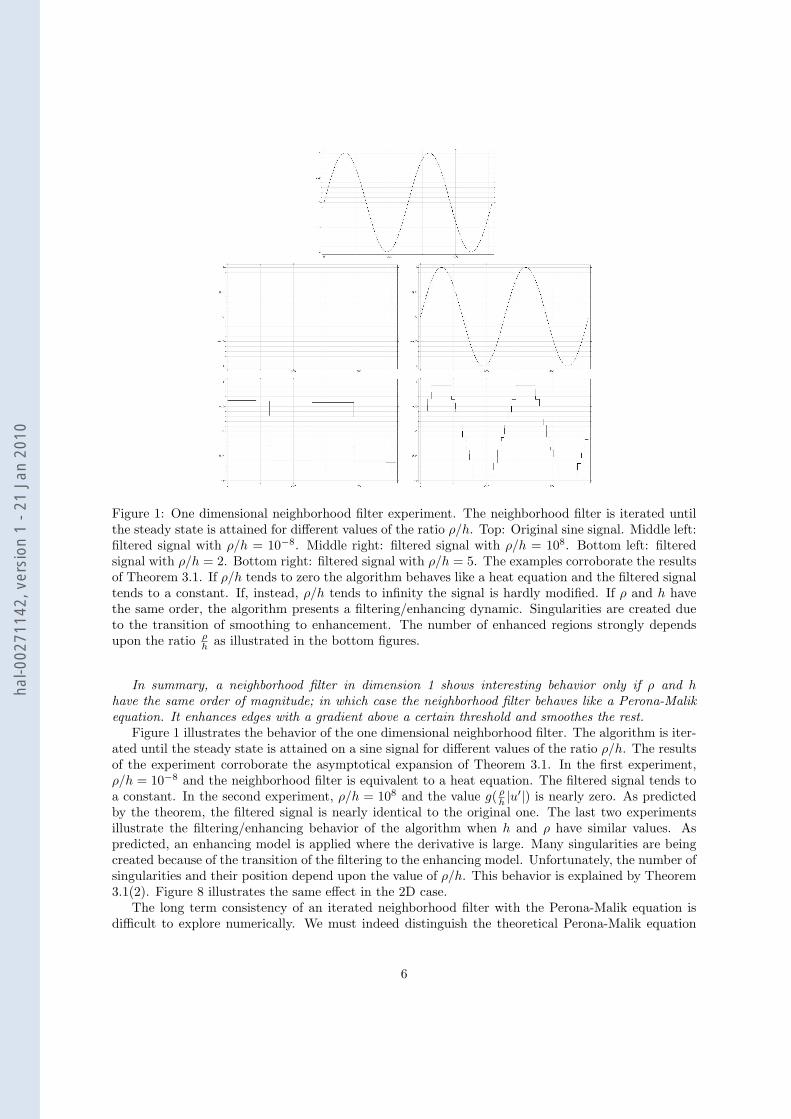
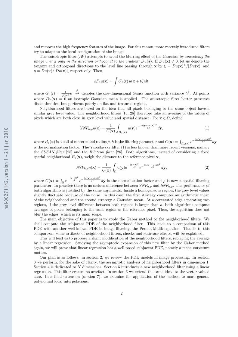
Figure 1: One dimensional neighborhood filter experiment. The neighborhood filter is iterated untilthe steady state is attained for different values of the ratio ρ/h. Top: Original sine signal. Middle left:filtered signal with ρ/h = 10−8. Middle right: filtered signal with ρ/h = 108. Bottom left: filteredsignal with ρ/h = 2. Bottom right: filtered signal with ρ/h = 5. The examples corroborate the resultsof Theorem 3.1. If ρ/h tends to zero the algorithm behaves like a heat equation and the filtered signaltends to a constant. If, instead, ρ/h tends to infinity the signal is hardly modified. If ρ and h havethe same order, the algorithm presents a filtering/enhancing dynamic. Singularities are created dueto the transition of smoothing to enhancement. The number of enhanced regions strongly dependsupon the ratio ρ

h as illustrated in the bottom figures.

In summary, a neighborhood filter in dimension 1 shows interesting behavior only if ρ and hhave the same order of magnitude; in which case the neighborhood filter behaves like a Perona-Malikequation. It enhances edges with a gradient above a certain threshold and smoothes the rest.

Figure 1 illustrates the behavior of the one dimensional neighborhood filter. The algorithm is iter-ated until the steady state is attained on a sine signal for different values of the ratio ρ/h. The resultsof the experiment corroborate the asymptotical expansion of Theorem 3.1. In the first experiment,ρ/h = 10−8 and the neighborhood filter is equivalent to a heat equation. The filtered signal tends toa constant. In the second experiment, ρ/h = 108 and the value g( ρ

h |u′|) is nearly zero. As predictedby the theorem, the filtered signal is nearly identical to the original one. The last two experimentsillustrate the filtering/enhancing behavior of the algorithm when h and ρ have similar values. Aspredicted, an enhancing model is applied where the derivative is large. Many singularities are beingcreated because of the transition of the filtering to the enhancing model. Unfortunately, the number ofsingularities and their position depend upon the value of ρ/h. This behavior is explained by Theorem3.1(2). Figure 8 illustrates the same effect in the 2D case.

The long term consistency of an iterated neighborhood filter with the Perona-Malik equation isdifficult to explore numerically. We must indeed distinguish the theoretical Perona-Malik equation

6

hal-0

0271

142,

ver

sion

1 -

21 J

an 2

010

from its numerical schemes. All finite diference schemes create some numerical diffusion. Thus,they are not exactly consistent with the Perona-Malik equation. This explains why iterating suchschemes can yield an asymptotic constant steady state. The Perona Malik equation is ill-posed andno existence-uniqueness theory is available to the best of our knowledge [1]. Now, it seems sound toconjecture that piecewise constant functions with smooth jumps could be steady states to the equationin a suitable existence theory. It is easy to check that such functions are also steady states to an iteratedneighborhood filter, provided the scale parameter is small enough. In summary, neighborhood filtersyield an implementation of the Perona-Malik consistent with piecewise constant steady states.

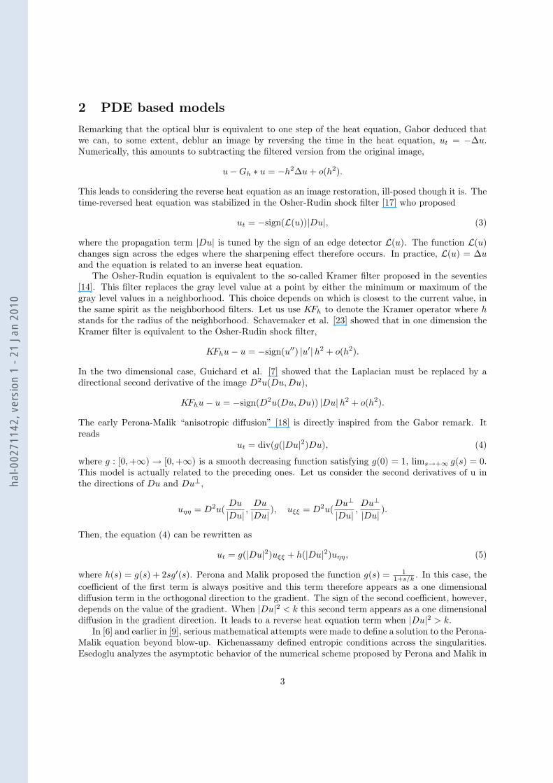
Figure 2: Comparison between the neighborhood filter and the shock filter. Top: Original signal.Bottom left: application of the neighborhood filter. Bottom right: application of the shock filter. Theminimum and the maximum of the signal have been preserved by the shock filter and reduced by theneighborhood filter. This fact illustrates the filtering/enhancing character of the neighborhood filtercompared with a pure enhancing filter.

The filtering/enhancing character of the neighborhood filter is very different from a pure enhancingalgorithm like the Osher-Rudin shock filter. Figures 2 and 3 illustrate these differences. In Figure2, the minimum and the maximum of the signal have been preserved by the shock filter, while thesetwo values have been significantly reduced by the neighborhood filter. This filtering/enhancing effectis optimal when the signal is noisy. Figure 3 shows how the shock filter creates artificial steps due tothe fluctuations of noise, while the neighborhood filter reduces the noise avoiding any spurious shock.Parameter h has been chosen larger than the amplitude of noise in order to remove it. Choosing anintermediate value of h, artificial steps could also be generated on points where the noise amplitudeis above this parameter value.

4 The N dimensional case

The previous theorem can be extended to the N-dimensional case, with the 2D and 3D case being themost interesting for image processing purposes. Films can also be modeled by a 3D spatiotemporalspace.

Let u(x1, . . . , xN ) be defined on a bounded domain Ω ⊂ RN and x ∈ Ω. Assume that Du(x) 6= 0and let us denote e1 = Du(x)/|Du(x)|. Let e2, . . . , eN be an orthonormal basis of the hyperplaneorthogonal to Du, Du⊥. Then the set e1, e2, . . . , eN forms an orthonormal basis of RN .

7

hal-0

0271

142,

ver

sion

1 -

21 J

an 2

010

Figure 3: Comparison between the neighborhood filter and the shock filter. Top: Original signal.Bottom left: application of the neighborhood filter. Bottom right: application of the shock filter. Theshock filter is sensitive to noise and creates spurious steps. The filtering/enhancing character of theneighborhood filter avoids this effect.

Theorem 4.1 Let u ∈ C2(Ω) and ρ, h, α > 0 such that ρ, h → 0 and h = O(ρα). Let us consider the

continuous function g defined by g(t) = 13

te−t2

E(t) , for t 6= 0, g(0) = 16 , where E(t) = 2

∫ t

0e−s2

ds. Let f

be the continuous function defined as

f(t) = 3g(t) +3g(t)

t2− 1

2t2, f(0) =

16.

Then, for x ∈ Ω,

1. If α < 1,

YNFh,ρu(x)− u(x) ' 4u(x)6

ρ2.

2. If α = 1,

YNFh,ρu(x)− u(x) '[f(

ρ

h|Du(x)|) D2u(e1, e1)(x)+

g(ρ

h|Du(x)|)

N∑

i=2

D2u(ei, ei)(x)

]ρ2

3. If 1 < α < 32 ,

YNFh,ρu(x)− u(x) ' g(ρ1−α|Du(x)|)[

3 D2u(e1, e1)(x) +N∑

i=2

D2u(ei, ei)(x)

]ρ2

Proof: First, we rewrite the difference YNFh,ρu(x)− u(x) as

YNFh,ρu(x)− u(x) =1

C(x)

∫

Bρ(0)

(u(x + t)− u(x))e−|u(x+t)−u(x)|2

h2 dt.

8

hal-0

0271

142,

ver

sion

1 -

21 J

an 2

010

Taking the Taylor expansion of u(x + t) for t ∈ Bρ(0),

u(x + t) = u(x) + pt1 +∑

i,j∈1,...,Nqijtitj + O(|t|3),

where t = (t1, . . . , tN ), p = |Du(x)| and if p > 0,

qii =12D2u(ei, ei)(x), qij = D2u(ei, ej)(x) if i 6= j.

When α < 1, we expand the exponential function and obtain

YNFh,ρu(x)− u(x) ' 1C(x)

∫

Bρ(0)

(pt1 +∑

i,j

qijtitj)(1− p2t21h2

) dt

' 14ρ2

24(x)uρ4

3.

This proves (1). When 1 ≤ α < 32 , we cannot apply the above expansion because ρ2

h2 does not tend tozero. However, ρ3

h2 → 0, and we can decompose the exponential as

e−|u(x+t)−u(x)|2

h2 = e−p2t21

h2 (1− 2pt1h2

∑

i,j

qijtitj + O(|t|4h2

)).

Using the Taylor expansion of u and of the above exponential function we obtain

YNFh,ρu(x)− u(x) ' 1C(x)

(∫

Bρ(0)

e−p2t21

h2 t21 dt− 2p2

h2

∫

Bρ(0)

e−p2t21

h2 t41 dt

)q11

+1

C(x)

N∑

i=2

(∫

Bρ(0)

e−p2t21

h2 t2i dt− 2p2

h2

∫

Bρ(0)

e−p2t21

h2 t21t2i dt

)qii

where C(x) ' ∫e−p2t21

h2 dt. Now, we compute the previous integrals and obtain

YNFh,ρu(x)− u(x) '2e

−p2t21h2

E(ρph )

ρp

h+

2e−p2t21

h2

E(ρph )

h

ρp− h2

ρ2p2

q11ρ

2 +2e

−p2t21h2

3E(ρph )

ρp

h

N∑

i=2

qiiρ2.

If h ' ρ, all the terms of the above expression have the same order ρ2 and rewriting them proves (2).When h ' ρα, 1 < α < 3

2 , we keep the lower order term and we get (3). ¤

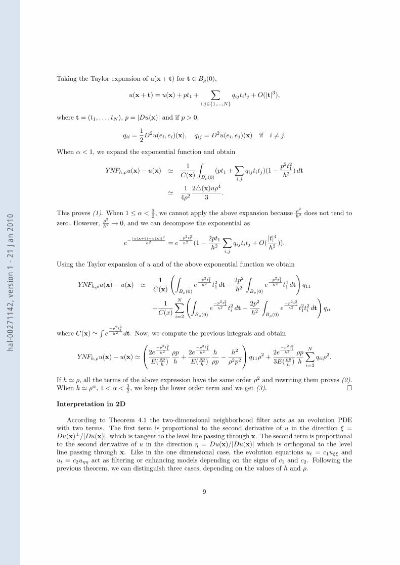
Interpretation in 2D

According to Theorem 4.1 the two-dimensional neighborhood filter acts as an evolution PDEwith two terms. The first term is proportional to the second derivative of u in the direction ξ =Du(x)⊥/|Du(x)|, which is tangent to the level line passing through x. The second term is proportionalto the second derivative of u in the direction η = Du(x)/|Du(x)| which is orthogonal to the levelline passing through x. Like in the one dimensional case, the evolution equations ut = c1uξξ andut = c2uηη act as filtering or enhancing models depending on the signs of c1 and c2. Following theprevious theorem, we can distinguish three cases, depending on the values of h and ρ.

9

hal-0

0271

142,

ver

sion

1 -

21 J

an 2

010

2 4 6 8

-0.1

-0.05

0.05

0.1

0.15

0.2

2 4 6 8

-0.1

-0.05

0.05

0.1

0.15

0.2

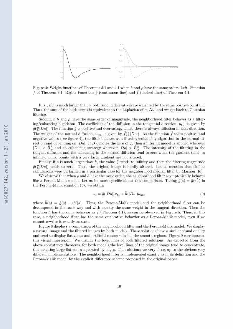
Figure 4: Weight functions of Theorems 3.1 and 4.1 when h and ρ have the same order. Left: Functionf of Theorem 3.1. Right: Functions g (continuous line) and f (dashed line) of Theorem 4.1.

First, if h is much larger than ρ, both second derivatives are weighted by the same positive constant.Thus, the sum of the both terms is equivalent to the Laplacian of u, ∆u, and we get back to Gaussianfiltering.

Second, if h and ρ have the same order of magnitude, the neighborhood filter behaves as a filter-ing/enhancing algorithm. The coefficient of the diffusion in the tangential direction, uξξ, is given byg( ρ

h |Du|). The function g is positive and decreasing. Thus, there is always diffusion in that direction.The weight of the normal diffusion, uηη, is given by f( ρ

h |Du|). As the function f takes positive andnegative values (see figure 4), the filter behaves as a filtering/enhancing algorithm in the normal di-rection and depending on |Du|. If B denotes the zero of f , then a filtering model is applied wherever|Du| < B h

ρ and an enhancing strategy wherever |Du| > B hρ . The intensity of the filtering in the

tangent diffusion and the enhancing in the normal diffusion tend to zero when the gradient tends toinfinity. Thus, points with a very large gradient are not altered.

Finally, if ρ is much larger than h, the value ρh tends to infinity and then the filtering magnitude

g( ρh |Du|) tends to zero. Thus, the original image is hardly altered. Let us mention that similar

calculations were performed in a particular case for the neighborhood median filter by Masnou [16].We observe that when ρ and h have the same order, the neighborhood filter asymptotically behaves

like a Perona-Malik model. Let us be more specific about this comparison. Taking g(s) = g(s12 ) in

the Perona-Malik equation (5), we obtain

ut = g(|Du|)uξξ + h(|Du|)uηη, (9)

where h(s) = g(s) + sg′(s). Thus, the Perona-Malik model and the neighborhood filter can bedecomposed in the same way and with exactly the same weight in the tangent direction. Then thefunction h has the same behavior as f (Theorem 4.1), as can be observed in Figure 5. Thus, in thiscase, a neighborhood filter has the same qualitative behavior as a Perona-Malik model, even if wecannot rewrite it exactly as such.

Figure 8 displays a comparison of the neighborhood filter and the Perona-Malik model. We displaya natural image and the filtered images by both models. These solutions have a similar visual qualityand tend to display flat zones and artificial contours inside the smooth regions. Figure 9 corroboratesthis visual impression. We display the level lines of both filtered solutions. As expected from theabove consistency theorems, for both models the level lines of the original image tend to concentrate,thus creating large flat zones separated by edges. The solutions are very close, up to the obvious verydifferent implementations. The neighborhood filter is implemented exactly as in its definition and thePerona-Malik model by the explicit difference scheme proposed in the original paper.

10

hal-0

0271

142,

ver

sion

1 -

21 J

an 2

010

1 2 3 4 5 6

-0.2

-0.1

0.1

0.2

Figure 5: Weight comparison of the neighborhood filter and the Perona Malik equation. Magnitude ofthe tangent diffusion (continuous line, identical for both models) and normal diffusion (dashed line ––) of Theorem 4.1. Magnitude of the tangent diffusion (continuous line) and normal diffusion (dashedline - - -) of the Perona-Malik model (9). Both models show nearly the same behavior.

5 A regression correction of the neighborhood filter

In the previous sections we have shown the enhancing character of the neighborhood filter. We haveseen that the neighborhood filter, like the Perona-Malik model, can create large flat zones and spuriouscontours inside smooth regions. This effect depends upon a gradient threshold which is hard to fixin such a way as to always separate the visually smooth regions from edge regions. In order to avoidthis undesirable effect, let us analyze in more detail what happens with the neighborhood filter in theone-dimensional case.

x

uHxLuHxL+h

uHxL-h

YNFHxLx- x+

Figure 6: Illustration of the shock effect of the YNF on the convex of a signal. The number of points ysatisfying u(x)− h < u(y) ≤ u(x) is larger than the number satisfying u(x) ≤ u(y) < u(x) + h. Thus,the average value Y NF (x) is smaller than u(x), enhancing that part of the signal. The regression lineof u inside (x−, x+) better approximates the signal at x.

Figure 6 shows a simple illustration of this effect. For each x in the convex part of the signal,the filtered value is the average of the points y such that u(x) − h < u(y) < u(x) + h for a certainthreshold h. As it is illustrated in the figure, the number of points satisfying u(x)−h < u(y) ≤ u(x) islarger than the number of points satisfying u(x) ≤ u(y) < u(x)+h. Thus, the average value Y NF (x)is smaller than u(x), enhancing this part of the signal. A similar argument can be applied in theconcave parts of the signal, dealing to the same enhancing effect. Therefore, shocks will be createdinside smooth zones where concave and convex parts meet. Figure 6 also shows how the mean is not

11

hal-0

0271

142,

ver

sion

1 -

21 J

an 2

010

a good estimate of u(x) in this case. In the same figure, we display the regression line approximatingu inside (u−1(u(x) − h), u−1(u(x) + h)). We see how the value of the regression line at x betterapproximates the signal. In the sequel, we propose to correct the neighborhood filter with this betterestimate.

In the general case, this linear regression strategy amounts to finding for every point x the hyper-plane locally approximating u in the following sense,

mina0,a1,...,aN

∫

Bρ(x)

w(x,y)(u(y)− aNyN − . . .− a1y1 − a0)2 dy, w(x,y) = e−|u(y)−u(x)|2

h2 (10)

and then replacing u(x) by the filtered value aNxN + . . . + a1x1 + a0. The weights used to define theminimization problem are the same as the ones used by the neighborhood filter. Thus, the points witha grey level value close to u(x) will have a larger influence in the minimization process than thosewith a further grey level value. We denote the above linear regression correction by LYNFh,ρ. Takinga1 = . . . = aN = 0 and then approximating u by a constant function, the minimization (10) goes backto the neighborhood filter.

In a more general framework, we can locally approximate image u by any polynomial. For anyn > 1, we can find the polynomial pn of degree n minimizing the following error,

minpn

∫

Bρ(x)

w(x, y)(u(y)− pn(y1, . . . , yN )2dy, w(x, y) = e−|u(y)−u(x)|2

h2 (11)

and define the filtered value at x as pn(x1, . . . , xN ). We denote the above polynomial regressioncorrection as LYNFn,h,ρ.

A similar scheme has been statistically studied in [22]. The authors propose an iterative procedurethat describes for every point the largest possible neighborhood in which the initial data can be wellapproximated by a parametric function.

Another similar strategy is the interpolation by ENO schemes [8]. The goal of ENO interpolationis to obtain a better adapted prediction near the singularities of the data. For each point it selectsdifferent stencils of fixed size M , and for each stencil reconstructs the associated interpolation poly-nomial of degree M . Then the least oscillatory polynomial is selected by some prescribed numericalcriterion. The selected stencils tend to escape from large gradients and discontinuities.

The regression strategy also tends to select the right points in order to approximate the function.Instead of choosing a certain interval, all the points are used in the polynomial reconstruction, butweighted by the grey level differences.

5.1 Linear regression

As in the previous sections, let us analyze the asymptotic behavior of the linear regression correction.We compute the asymptotic expansion of the filter when 0 < α ≤ 1. We showed that when α > 1 thesignal is hardly modified.

For the sake of completeness, we first compute the asymptotic expansion in the one dimensionalcase. We omit the proof of this result since it can be easily obtained from the next proof in theN-dimensional case.

Theorem 5.1 Suppose u ∈ C2(I), and let ρ, h, α > 0 such that ρ, h → 0 and h = O(ρα). Let f bethe continuous function defined as f(0) = 1

6 ,

f(t) =1

4t2

(1− 2t e−t2

E(t)

),

for t 6= 0, where E(t) = 2∫ t

0e−s2

ds. Then, for x ∈ R,

12

hal-0

0271

142,

ver

sion

1 -

21 J

an 2

010

1. If α < 1, LYNFh,ρu(x)− u(x) ' u′′(x)6 ρ2.

2. If α = 1, YNFh,ρu(x)− u(x) ' f( ρh |u′(x)|)u′′(x) ρ2.

Theorem 5.1 shows that the LYNFh,ρ filter lets the signal evolve proportionally to its secondderivative, as the neighborhood filter does. When h is larger than ρ the filter is equivalent to theoriginal neighborhood filter and the signal is filtered by a heat equation. When ρ and h have thesame order the sign and magnitude of the filtering process is given by f( ρ

h |u′(x)|) (see Figure 7). Thisfunction is positive and quickly decreases to zero. Thus, the signal is filtered by a heat equation ofdecreasing magnitude and is not altered wherever the derivative is very large.

The same asymptotic expansion can be computed in the N-dimensional case. Let e1 = Du(x)/|Du(x)|and take e2, . . . , eN as an orthonormal basis of the hyperplane orthogonal to Du, Du⊥. Then the sete1, e2, . . . , eN forms an orthonormal basis of RN .

Theorem 5.2 Suppose u ∈ C2(Ω), and let ρ, h, α > 0 such that ρ, h → 0 and h = O(ρα). Let f bethe continuous function defined as f(0) = 1

6 ,

f(t) =1

4t2

(1− 2t e−t2

E(t)

),

for t 6= 0, where E(t) = 2∫ t

0e−s2

ds. Then, for x ∈ Ω,

1. If α < 1,

LYNFh,ρu(x)− u(x) ' 4u(x)6

ρ2.

2. If α = 1,

LYNFh,ρu(x)− u(x) '[f(

ρ

h|Du(x)|) D2u(e1, e1)(x) +

16

N∑

i=2

D2u(ei, ei)

]ρ2

Proof: The solution of the minimization process (10) leads to the resolution of the linear systemAx = b,

A =

a(2, 0, . . . , 0) a(1, 1, . . . , 0) . . . a(1, 0, . . . , 1) a(1, 0, . . . , 0)a(1, 1, . . . , 0) a(0, 2, . . . , 0) . . . a(0, 1, . . . , 1) a(0, 1, . . . , 0)

.... . .

...a(1, 0, . . . , 1) a(0, 1, . . . , 1) . . . a(0, . . . , 0, 2) a(0, 0, . . . , 1)a(1, 0, . . . , 0) a(0, 1, . . . , 0) . . . a(0, 0, . . . , 1) a(0, 0, . . . , 0)

b =

b(1, 0, . . . , 0)b(0, 1, . . . , 0)

...b(0, 0, . . . , 1)b(0, 0, . . . , 0)

wherea(α1, . . . , αN ) =

∫

Bρ(x)

tα11 . . . tαN

N w(t1, . . . , tN ) dt1 . . . dtN ,

b(α1, . . . , αN ) =∫

Bρ(x)

tα11 . . . tαN

N u(t1, . . . , tN ) w(t1, . . . , tN ) dt1 . . . dtN ,

x = (x1, . . . , xN ) and w(t1, . . . , tN ) = e−|u(t1,...,tN )−u(x1,...,xN )|2

h2 .We can suppose, without loss of generality, that x = 0. In this case, LYNFh,ρu(0) = a0 can be

written as det A′/det A, where A is defined above and A′ is obtained by replacing the last column ofA by b. Now, by taking the function u(t) = u(t)− u(0) we can rewrite

b(α1, . . . , αN ) = b(α1, . . . , αN ) + u(0) a(α1, . . . , αN ),

13

hal-0

0271

142,

ver

sion

1 -

21 J

an 2

010

and det A′ can be decomposed as det A + u(0) detA. Then the difference between the filtered andoriginal images is

LYNFh,ρu(0)− u(0) =det A + u(0) detA

detA− u(0) =

det A

det A.

We take the Taylor expansion of u(t) for t ∈ Bρ(0),

u(t) = u(0) + pt1 +∑

i,j∈1,...,Nqijtitj + O(|t|3),

where t = (t1, . . . , tN ), p = |Du(0)| and if p > 0,

qii =12D2u(ei, ei), qij = D2u(ei, ej) if i 6= j.

When α < 1, we apply the usual Taylor expansion of the exponential function. The terms of lowerorder of matrices A and A are in their diagonal and the quotient can be approximated by the lowerterms of

b(0, 0, . . . , 0)a(0, 0, . . . , 0)

.

Therefore, the analysis of the difference reduces to the computation of the two terms,

a(0, . . . , 0) '∫

Bρ(0)

dt1 . . . dtN ' 2NρN

b(0, . . . , 0) 'N∑

i=1

qii

∫

Bρ(0)

t2i dt1 . . . dtN =2NρN+2

6∆u

This proves (1).When α = 1, we cannot apply the above expansion because ρ2

h2 does not tend to zero. However,ρ3

h2 → 0, and we can decompose the exponential as

e−|u(t)−u(0)|2

h2 = e−p2t21

h2

1− 2pt1

h2

∑

i,j

qijtitj + O(|t|4h2

)

.

The lower order terms of the matrices A and A are the diagonal elements, a(1, 0, . . . , 0) and b(1, 0, . . . , 0).Then, the lower order terms of the quotient are given by

det A

detA' b(0, . . . , 0)

∏Ni=1 a(0, . . . ,

(i)

2 , . . . , 0)− b(1, 0, . . . , 0)a(1, 0, . . . , 0)∏N

i=2 a(0, . . . ,(i)

2 , . . . , 0)

a(0, . . . , 0)∏N

i=1 a(0, . . . ,(i)

2 , . . . , 0)

=b(0, . . . , 0)a(2, 0, . . . , 0)− b(1, 0, . . . , 0)a(1, 0, . . . , 0)

a(0, . . . , 0)a(2, 0, . . . , 0). (12)

Therefore, the analysis of the difference reduces to the computation of the terms,

a(0, . . . , 0) '∫

Bρ(0)

e−p2t21

h2 dt1 . . . dtN

14

hal-0

0271

142,

ver

sion

1 -

21 J

an 2

010

a(1, 0, . . . , 0) ' −2p

h2

N∑

i=1

qii

∫

Bρ(0)

e−p2t21

h2 t21 t2i dt1 . . . dtN

a(2, 0, . . . , 0) '∫

Bρ(0)

e−p2t21

h2 t21 dt1 . . . dtN

b(0, . . . , 0) 'N∑

i=1

qii

∫

Bρ(0)

e−p2t21

h2 t2i dt1 . . . dtN − 2p2

h2

N∑

i=1

qii

∫

Bρ(0)

e−p2t21

h2 t21t2i dt1 . . . dtN

b(1, 0, . . . , 0) ' p

∫

Bρ(0)

e−p2t21

h2 t21 dt1 . . . dtN .

Now, replacing the terms in (12) by the previous estimates we get

LYNFh,ρu(0)− u(0) ' q11

∫Bρ(0)

e−p2t21

h2 dt1 . . . dtN

∫

Bρ(0)

e−p2t21

h2 t21 dt1 . . . dtN

+N∑

i=2

qii

∫Bρ(0)

e−p2t21

h2 dt1 . . . dtN

∫

Bρ(0)

e−p2t21

h2 t2i dt1 . . . dtN .

Computing the previous integrals and taking into account that O(ρ) = O(h) we prove (2). ¤

Interpretation in 2DAccording to the previous theorem, the filter can be written as the sum of two diffusion terms in thedirection of ξ and η. When h is much larger than ρ the linear regression correction is equivalent to theheat equation like the original neighborhood filter. When ρ and h have the same order, the behaviorof the linear regression algorithm is very different from the original neighborhood filter. The functionweighting the tangent diffusion is a positive constant. The function weighting the normal diffusionis positive and decreasing (see figure 7), and therefore there is no enhancing effect. The algorithmcombines the tangent and normal diffusion wherever the gradient is small. Wherever the gradient islarger the normal diffusion is canceled and the image is filtered only in its tangent direction. Thissubjacent PDE was already proposed as a diffusion equation in [13]. This diffusion makes the levellines evolve proportionally to their curvature. In the Perona-Malik model the diffusion is stopped nearthe edges. In this case, the edges are filtered by a mean curvature motion.

It may be asked whether the modified neighborhood filter still preserves signal discontinuities. Theanswer is yes. It is easily checked that for small enough h, all piecewise affine functions with smoothjump curves are steady. Thus, the behavior is the same as for the classical neighborhood filter. Ourasymptotic analysis is of course not valid for such functions, but only for smooth functions.

As a numerical scheme the linear regression neighborhood filter allows the implementation of amean curvature motion without the computation of gradients and orientations. When the gradientis small the linear regression filter naturally behaves like the heat equation. This effect is introducedon typical schemes implementing the mean curvature motion. In flat zones the gradient is not welldefined and some kind of isotropic diffusion must be applied. Therefore, the linear regression neigh-borhood filter naturally extends the mean curvature motion and yields a stable numerical scheme forits computation, independent of gradient orientations.

Figure 8 displays an experiment comparing the LYNFh,ρ with the neighborhood filter and thePerona-Malik equation. The linear correction does not create any contour or flat zone inside thesmooth regions. Figure 9 displays the level lines of the previous experiment. The level lines of theLYNFh,ρ are filtered by a mean curvature motion and they do not get grouped creating flat zones.

15

hal-0

0271

142,

ver

sion

1 -

21 J

an 2

010

2 4 6 8 10

0.05

0.1

0.15

0.2

0.25

2 4 6 8 10

0.05

0.1

0.15

0.2

0.25

Figure 7: Weighting functions of Theorem 5.1 and 5.2. Left: Function f of Theorem 5.1. Right:Constant function 1/6 (continuous line) and function f (dashed line) of Theorem 5.2.

In the N -dimensional case, we can choose e2, . . . , eN to be a basis of eigenvectors of D2u(x)restricted to Du(x)⊥. In this case the diffusion terms are equal to the principal curvatures of thelevel surface passing through x, and their sum gives the mean curvature operator. Therefore whenthe gradient is above a certain threshold the linear regression neighborhood filter is equivalent to theN -dimensional mean curvature motion.

Figure 10 shows a benefit of the linear regression correction in the three-dimensional case. Weapply the neighborhood filter to the 3D image u(x, y, z) = x2 + y2 + z2 − r2. The zero level set of uis the boundary of the sphere of radius r. We should expect this level set to evolve isotropically andto preserve its sphere form, which is not the case when applying the neighborhood filter. This effectis avoided by the linear regression which makes the zero level set evolve uniformly and preserve theisotropy of the initial data.

5.2 The action of the regression filter on image sequences

Classical movie filtering techniques usually compute an optical flow estimate of the sequence as aprevious step. The optical flow associates to each point a vector representing its optical velocity,v = (vx, vy) (we denote v = (vx, vy, 1)). If ∆t is the time interval between two consecutive frames,x+v(x)∆t denotes the point shifted by v(x) in the next frame. The optical flow estimation gives thetheoretical trajectories of each pixel along the sequence. Thus, denoising a pixel should be performedby averaging its computed trajectory.

The classical definition of the optical flow involves the Lambertian assumption that physical pointsmaintain the same grey level value when the camera moves,

u(x + v(x)∆t) ' u(x),

which is equivalent to saying that v(x) ·Du(x) = 0. Therefore, the conservation assumption only tellsus that the velocity vector is contained in the plane Du⊥. Some additional criteria must be addedin order to achieve the uniqueness of the trajectories. Theorem 5.2 shows that when the gradient isabove a certain threshold the linear regression neighborhood filter performs a diffusion in the planeDu⊥. Thus, instead of choosing pixels of the trajectory for the averaging process, which would requirea solution to the ambiguity of trajectories, the algorithm makes an average of all the points with asimilar grey level value.

The enhancing effect of the neighborhood filter is aggravated by the presence of noise. The irregu-larities of the edges due to the noise are enhanced and lead to very irregular and oscillatory contours.This effect is even more annoying when dealing with films. The irregularities of a given edge aredifferent from frame to frame, leading to a false motion impression when the sequence is played. InFigure 12 we display two consecutive frames of a noisy image sequence. We display the same framesonce the sequence has been filtered by the neighborhood filter and its linear correction. On comparingthe single images we observe that the edges of the filtered sequence by the neighborhood filter are

16

hal-0

0271

142,

ver

sion

1 -

21 J

an 2

010

Figure 8: Comparison experiment. Top left: original image. Top right: Perona-Malik filtered image.Bottom left: filtered image by the neighborhood filter. Bottom right: filtered image by the linearregression neighborhood filter. The neighborhood filter experiments are performed by iterating thediscrete version of definitions (1) and (10). Both the neighborhood filter and its linear regressioncorrection have been applied with the same value of h and ρ. The displayed images have been attainedwithin the same number of iterations. The Perona-Malik equation is implemented by the explicitdifference scheme proposed in the original paper. The Perona-Malik model and the neighborhoodfilter create artificial contours and flat zones. This effect is almost completely avoided by the linearregression neighborhood filter.

much more irregular than the original ones. The linear regression correction avoids this effect andregularizes the edges. Finally, we display for each filtered sequence the difference between the twoconsecutive frames for each filtered sequence. The edges are less noticeable in the frame difference ofthe linear regression correction, that is, the oscillations from frame to frame are reduced.

6 The vector valued case

Let u be a vector valued function defined on a bounded domain Ω ⊂ R2, u : Ω → Rn. The vectorneighborhood filter can be written as

YNFh,ρu(x) =1

C(x)

∫

Bρ(x)

u(y)e−||u(y)−u(x)||2

h2 dy, (13)

where ||u(y) − u(x)||2 is now the Euclidean vector norm and each component function ui is filteredwith the same weight distribution. The linear regression correction is defined as in the scalar case,

17

hal-0

0271

142,

ver

sion

1 -

21 J

an 2

010

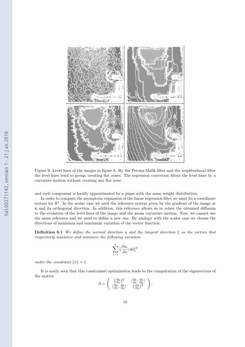
Figure 9: Level lines of the images in figure 8. By the Perona-Malik filter and the neighborhood filterthe level lines tend to group, creating flat zones. The regression correction filters the level lines by acurvature motion without creating any flat zone.

and each component is locally approximated by a plane with the same weight distribution.In order to compute the asymptotic expansion of the linear regression filter we must fix a coordinate

system for R2. In the scalar case we used the reference system given by the gradient of the image atx and its orthogonal direction. In addition, this reference allows us to relate the obtained diffusionto the evolution of the level lines of the image and the mean curvature motion. Now, we cannot usethe same reference and we need to define a new one. By analogy with the scalar case we choose thedirections of minimum and maximum variation of the vector function.

Definition 6.1 We define the normal direction η and the tangent direction ξ as the vectors thatrespectively maximize and minimize the following variation

n∑

i=1

‖∂ui

∂v(x)‖2

under the constraint ‖v‖ = 1.

It is easily seen that this constrained optimization leads to the computation of the eigenvectors ofthe matrix

A =

(‖∂u

∂x‖2 〈∂u∂x , ∂u

∂y 〉〈∂u

∂x , ∂u∂y 〉 ‖∂u

∂y ‖2)

,

18

hal-0

0271

142,

ver

sion

1 -

21 J

an 2

010

Figure 10: Evolution of a 3D sphere by the linear regression neighborhood filter. Left: Zero level set ofu(x, y, z) = x2 + y2 + z2− r2 (sphere of radius r). Middle: Zero level set of u after the iteration of theneighborhood filter. Right: Zero level set of u after the iteration of the linear regression neighborhoodfilter. The linear regression makes the zero level set evolve uniformly and preserves the isotropicproperty of the initial data, which is not the case of the neighborhood filter.

where ∂u∂x =

(∂u1∂x , . . . , ∂un

∂x

)and ∂u

∂y =(

∂u1∂y , . . . , ∂un

∂y

). The two positive eigenvalues of A, λ+ and λ−,

are the maximum and the minimum of the vector norm associated to A and the maximum and theminimum variations as defined in Definition 6.1. The corresponding eigenvectors are orthogonal lead-ing to the above defined normal and tangent directions. This orthonormal system was first proposedfor vector valued image analysis in [5]. Many PDE equations have been proposed for color imagefiltering using this system. We note the Coherence Enhancing Diffusion [27], the Beltrami Flow [11]and an extension of the mean curvature motion [21].

Theorem 6.1 Suppose u ∈ C2(Ω,Rn), and let ρ, h, α > 0 such that ρ, h → 0 and h = O(ρα). Let fbe the continuous function defined as f(0) = 1

6 ,

f(t) =1

4t2

(1− 2t e−t2

E(t)

),

for t 6= 0, where E(t) = 2∫ t

0e−s2

ds. Then, for x ∈ Ω,

1. If α < 1,

LYNFh,ρu(x)− u(x) ' 4u(x)6

ρ2.

2. If α = 1,

LYNFh,ρu(x)− u(x) '[f(

ρ

h‖∂u

∂ξ(x)‖) D2u(ξ, ξ)(x) + f(

ρ

h‖∂u

∂η(x)‖)D2u(η, η)(x)

]ρ2

where ∆u(x) = (∆ui(x))1≤i≤n and D2u(v, v)(x) =(D2ui(v, v)(x)

)1≤i≤n

for v ∈ η, ξ.

Proof: Let u0 denote an arbitrary component of u and let us suppose without loss of generality thatx = 0. In this case, the same argument of the proof of Theorem 5.2 shows that

LYNFh,ρu0(0)− u(0) =det A

detA,

where

A =

a(2, 0) a(1, 1) a(1, 0)a(1, 1) a(0, 2) a(0, 1)a(1, 0) a(0, 1) a(0, 0)

, A =

a(2, 0) a(1, 1) b(1, 0)a(1, 1) a(0, 2) b(0, 1)a(1, 0) a(0, 1) b(0, 0)

19

hal-0

0271

142,

ver

sion

1 -

21 J

an 2

010

anda(α1, α2) =

∫

Bρ(0)

tα11 tα2

2 w(t1, t2) dt1dt2,

b(α1, α2) =∫

Bρ(0)

tα11 tα2

2 w(t1, t2) [u0(t1, t2)− u0(0)] dt1dt2.

The weight function w(t1, t2) depends on the differences |ui(t1, t2)− ui(0)|, for i = 1, . . . , n,

w(t1, t2) = e−1

h2Pn

i=1 |ui(t1,t2)−ui(0,0)|.

We take the Taylor expansion of u0(t) and ui(t) for t ∈ Bρ(0),

ui(t) = ui(0) + piξt1 + piη

t2 + qiξξt21 + qiηη

t22 + qiξηt1t2 + O(|t|3),

where t = (t1, t2), piξ= ∂ui

∂ξ , piη= ∂ui

∂η and

qiξξ=

12D2ui(ξ, ξ), qiηη

=12D2ui(η, η) and qiξη

= D2ui(ξ, η).

When α < 1, we apply the usual Taylor expansion of the exponential function. The lower orderterms of matrices A and A are in their diagonal and the quotient can be approximated by the lowerterms of b(0, 0)/a(0, 0). Therefore, the analysis of the difference reduces to the computation of thetwo terms,

a(0, 0) '∫

Bρ(0)

dt1dt2 ' 4ρ2

b(0, 0) '∫

Bρ(0)

(q0ξξt21 + q0ηη t22) dt1dt2 =

4∆u0

6ρ4

This proves (1).When α = 1, we cannot apply the above expansion and we decompose the weight function as

w(t1, t2) ' e−1

h2 (a2t21+b2t22)

(1− 1

h2(c30t

31 + c21t

21t2 + c12t1t

22 + c03t

32)

),

wherea = ‖∂u

∂ξ‖, b = ‖∂u

∂η‖, c30 = 2〈D2u(ξ, ξ),

∂u

∂ξ〉, c03 = 2〈D2u(η, η),

∂u

∂η〉,

c21 = 2〈D2u(ξ, η),∂u

∂ξ〉+ 2〈D2u(ξ, ξ),

∂u

∂η〉, c12 = 2〈D2u(ξ, η),

∂u

∂η〉+ 2〈D2u(η, η),

∂u

∂ξ〉.

We do not have a crossed term in the exponential function thanks to the orthogonality of ∂u∂ξ and ∂u

∂η .The lower order terms of the matrices A and A are the diagonal elements, a(1, 0), a(0, 1), b(1, 0) andb(0, 1). Then, the lower order terms of the quotient are given by

det A

detA' a(2, 0)a(0, 2)b(0, 0)− a(1, 0)a(0, 2)b(1, 0)− a(2, 0)a(0, 1)b(0, 1)

a(2, 0)a(0, 2)a(0, 0). (14)

Therefore, the analysis of the difference reduces to the computation of the terms,

a(0, 0) '∫

Bρ(0)

e−1

h2 (a2t21+b2t22) dt1dt2,

20

hal-0

0271

142,

ver

sion

1 -

21 J

an 2

010

a(1, 0) ' − 1h2

∫

Bρ(0)

(c30t41 + c12t

21t

22) e−

1h2 (a2t21+b2t22) dt1dt2,

a(0, 1) ' − 1h2

∫

Bρ(0)

(c03t42 + c21t

21t

22) e−

1h2 (a2t21+b2t22) dt1dt2,

a(2, 0) '∫

Bρ(0)

t21 e−1

h2 (a2t21+b2t22) dt1dt2, a(0, 2) '∫

Bρ(0)

t22 e−1

h2 (a2t21+b2t22) dt1dt2,

b(1, 0) ' p0ξ

∫

Bρ(0)

t21 e−1

h2 (a2t21+b2t22) dt1dt2, b(0, 1) ' p0η

∫

Bρ(0)

t22 e−1

h2 (a2t21+b2t22) dt1dt2,

b(0, 0) '∫

Bρ(0)

(q0ξξt21 + q0ηη t22)e

− 1h2 (a2t21+b2t22) dt1dt2

− 1h2

∫

Bρ(0)

(p0ξc30t

41 + p0η

c03t42 + (p0ξ

c12 + p0ηc21)t21t

22) e−

1h2 (a2t21+b2t22) dt1dt2,

Now, replacing the terms in (14) by the previous estimates we get

1∫Bρ(0)

e−1

h2 (a2t21+b2t22) dt1dt2

∫

Bρ(0)

(q0ξξt21 + q0ηη t22) e−

1h2 (a2t21+b2t22) dt1dt2.

Computing the previous integrals and taking into account that O(ρ) = O(h) we prove (2). ¤

InterpretationWhen h is much larger than ρ, the linear regression neighborhood filter is equivalent to the heatequation applied independently to each component. When h and ρ have the same order the subjacentPDE acts as an evolution equation with two terms. The first term is proportional to the secondderivative of u in the tangent direction ξ. The second term is proportional to the second derivativeof u in the normal direction η. The magnitude of each diffusion term depends on the variation inthe respective direction, λ− = ‖∂u

∂ξ (x)‖ and λ+ = ‖∂u∂η (x)‖. The weighting function f is positive and

decreases to zero (see Figure 7). We can distinguish the following cases depending on the values ofλ+ and λ−.

• If λ+ ' λ− ' 0 then there are very few variations of the vector image u around x. In this case,the linear regression neighborhood filter behaves like a heat equation with maximum diffusioncoefficient f(0).

• If λ+ >> λ− then there are strong variations of u around x and the point may be located on anedge. In this case the magnitude f( ρ

hλ+) tends to zero and there is no diffusion in the directionof maximal variation. If λ− >> 0 then x may be placed on an edge with different orientationsdepending on each component and the magnitude of the filtering in both directions tends tozero, so that the image is hardly altered. If λ− ' 0 then the edges have similar orientationsin all the components and the image is filtered by a directional Laplacian in the direction ofminimal variation.

• If λ+ ' λ− >> 0 then we may be located on a saddle point and in this case the image is hardlymodified. When dealing with multi-valued images one can think of the complementarity of thedifferent channels leading to the perception of a corner.

21

hal-0

0271

142,

ver

sion

1 -

21 J

an 2

010

In the scalar case the theorem gives back the result studied in the previous sections. The normaland tangent directions are respectively the gradient direction and the level line direction. In this case,∂u∂ξ (x) = 0 and ∂u

∂η (x) = |Du(x)| and we get back to

LYNFh,ρu(x)− u(x) '[16D2u(ξ, ξ)(x) + f(

ρ

h|Du(x)|)D2u(η, η)(x)

]ρ2.

7 The Polynomial Regression

In this section, we extend the previous asymptotic analysis to the polynomial regression defined in(11). First, we compute the asymptotic expansion for the polynomials of degree 2. We only analyzethe two dimensional case since we are mainly interested in its interpretation for image filtering.

Theorem 7.1 Suppose u ∈ C2(Ω), and let ρ, h, α > 0 such that ρ, h → 0 and h = O(ρα). Let

f(t) =4 t2

(−3 + t2)

+ 2 et2 t(6− t2 + 2 t4

)E(t)− 3 e2 t2 E(t)2

96 t4(2 t2 + et2 t (1 + 2 t2) E(t)− e2 t2 E(t)2

) ,

and

g(t) =1

36t2

(1− 2 t e−t2

E(t)

)

for t 6= 0, where E(t) = 2∫ t

0e−s2

ds. Then, for x ∈ Ω,

1. If α < 1,

YNF2,h,ρu(x)− u(x) ' −[

1280

uηηηη +154

uηηξξ +1

280uξξξξ

]ρ4

2. If α = 1,

LYNF2,h,ρu(x)− u(x) ' −[f(

ρ

h|Du(x)|)uηηηη + g(

ρ

h|Du(x)|)uηηξξ +

1280

uξξξξ

]ρ4

+c[f1(

ρ

h|Du(x)|)uηηη + f2(

ρ

h|Du(x)|)uηξξ

]uηη ρ4

+c[f3(

ρ

h|Du(x)|)uξξξ + f4(

ρ

h|Du(x)|)uηηξ

]uηξ ρ4

+c[f5(

ρ

h|Du(x)|)uηηη + f6(

ρ

h|Du(x)|)uηξξ

]uξξ ρ4

where c denotes ρ/h. The graphs of the functions f1, . . . , f6 are plotted in figure 11.

The proof of the theorem follows the same scheme as previous results. However, the large numberof terms and the complexity of the weighting functions make it impossible to write the proof on paper.The graphs of the functions involved in the theorem are plotted in Figure 11.

The polynomial approximation better adapts to the local image configuration than the linear ap-proximation. The order obtained by the polynomial regression of degree 2 is ρ4 while the neighborhoodfilter and its linear correction raised an order ρ2.InterpretationWhen h is much larger than ρ the image is filtered by a nearly isotropic diffusion. The diffusion iswritten as a constant combination of uηηηη, uξξξξ and uηηξξ. To the best of our knowledge, there is

22

hal-0

0271

142,

ver

sion

1 -

21 J

an 2

010

1 2 3 4 5 6

0.005

0.01

0.015

0.02

1 2 3 4 5 6

0.002

0.004

0.006

0.008

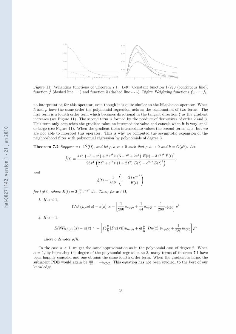
Figure 11: Weighting functions of Theorem 7.1. Left: Constant function 1/280 (continuous line),function f (dashed line – –) and function g (dashed line - - -). Right: Weighting functions f1, . . . , f6.

no interpretation for this operator, even though it is quite similar to the bilaplacian operator. Whenh and ρ have the same order the polynomial regression acts as the combination of two terms. Thefirst term is a fourth order term which becomes directional in the tangent direction ξ as the gradientincreases (see Figure 11). The second term is formed by the product of derivatives of order 2 and 3.This term only acts when the gradient takes an intermediate value and cancels when it is very smallor large (see Figure 11). When the gradient takes intermediate values the second terms acts, but weare not able to interpret this operator. This is why we computed the asymptotic expansion of theneighborhood filter with polynomial regression by polynomials of degree 3.

Theorem 7.2 Suppose u ∈ C2(Ω), and let ρ, h, α > 0 such that ρ, h → 0 and h = O(ρα). Let

f(t) =4 t2

(−3 + t2)

+ 2 et2 t(6− t2 + 2 t4

)E(t)− 3 e2 t2 E(t)2

96 t4(2 t2 + et2 t (1 + 2 t2) E(t)− e2 t2 E(t)2

) ,

and

g(t) =1

36t2

(1− 2 t e−t2

E(t)

)

for t 6= 0, where E(t) = 2∫ t

0e−s2

ds. Then, for x ∈ Ω,

1. If α < 1,

YNF3,h,ρu(x)− u(x) ' −[

1280

uηηηη +154

uηηξξ +1

280uξξξξ

]ρ4

2. If α = 1,

LYNF3,h,ρu(x)− u(x) ' −[f(

ρ

h|Du(x)|)uηηηη + g(

ρ

h|Du(x)|)uηηξξ +

1280

uξξξξ

]ρ4

where c denotes ρ/h.

In the case α < 1, we get the same approximation as in the polynomial case of degree 2. Whenα = 1, by increasing the degree of the polynomial regression to 3, many terms of theorem 7.1 havebeen happily canceled and one obtains the same fourth order term. When the gradient is large, thesubjacent PDE would again be ∂u

∂t = −uξξξξ. This equation has not been studied, to the best of ourknowledge.

23

hal-0

0271

142,

ver

sion

1 -

21 J

an 2

010

8 Conclusion

Our first aim was to understand neighborhood filters thanks to their asymptotic PDE behavior. Thisled us to improve these filters by using the well-posed nature of the PDE as a cue. Conversely, thisstudy introduced neighborhood filters as new kinds of numerical schemes for classical PDE’s like thePerona-Malik or the mean curvature motion. The study led to two equations of interest,

∂u

∂t= −uξξξξ

and∂u

∂t= −

[1

280uηηηη +

154

uηηξξ +1

280uξξξξ

]

where ξ is the direction orthogonal to the gradient and η the direction of the gradient. We know ofno existence theory for these equations. The two preceding theorems give them consistent numericalschemes.

References

[1] H. Amann, ”A new approach to quasilinear parabolic problems”, International Confererence onDifferential Equations, 2005.

[2] F. Andreu, C. Ballester, V. Caselles and J. M. Mazı¿12 , ”Minimizing Total Variation Flow”, Dif-

ferential and Integral Equations, 14 (3), pp. 321-360, 2001.

[3] D. Barash, ”A Fundamental Relationship between Bilateral Filtering, Adaptive Smoothing and theNonlinear Diffusion Equation”, IEEE Transactions on Pattern Analysis and Machine Intelligence24 (6), 2002.

[4] T.F. Chan, S. Esedoglu, F.E. Park, ”Image Decomposition Combining Staircase Reduction andTexture Extraction”, Preprint CAM-18, UCLA, 2005.

[5] S. Di Zenzo. ”A note on the gradient of a multi-image”. Computer Vision, Graphics, and ImageProcessing, vol. 33, pp. 116-125, 1986.

[6] S. Esedoglu, ”An analysis of the Perona-Malik scheme”, Communications on Pure and AppliedMathematics, vol. 54, pp. 1442-1487, 2001.

[7] F. Guichard and J.M Morel, ”A Note on Two Classical Enhancement Filters and Their AssociatedPDE’s”, International Journal of Computer Vision, Volume 52 (2-3), pp. 153-160, 2003.

[8] A. Harten, B. Enquist, S. Osher and S. Chakravarthy, ”Uniformly high order accurate essentiallynon-oscillatory schemes III”, Journal of Computational Physics, vol. 71, pp. 231-303, 1987.

[9] S. Kichenassamy, ”The Perona-Malik paradox”, SIAM Journal Applied Mathematics, vol. 57 (2),pp. 1328-1342, 1997.

[10] B.B. Kimia, A. Tannenbaum, and S.W. Zucker, ”On the evolution of curves via a function ofcurvature I the classical case”, Journal of Mathematical Analysis and Applications, 163(2), pp.438-458, 1992.

[11] R. Kimmel, R. Malladi, and N. Sochen, ”Images as embedded maps and minimal surfaces: movies,color, texture, and volumetric medical images”, International Journal of Computer Vision, vol.39(2), pp. 111-129, 2000.

24

hal-0

0271

142,

ver

sion

1 -

21 J

an 2

010

[12] S. Kindermann, S. Osher and P. Jones, ”Deblurring and Denoising of Images by Nonlocal Func-tionals”, UCLA Computational and Applied Mathematics Reports, 04-75, 2004.

[13] P. Kornprobst, ”Contributions ı¿12 la Restauration d’Images et l’Analyse de Sı¿1

2uences: Ap-proches Variationnelles et Solutions de Viscositı¿1

2 . PhD thesis, Universitı¿12 de Nice-Sophia An-

tipolis, 1998.

[14] H. P. Kramer and J. B Bruckner. ”Iterations of a non-linear transformation for enhancement ofdigital images”. Pattern Recognition, 7, 1975.

[15] J.S. Lee ”Digital image smoothing and the sigma filter”, Computer Vision, Graphics, and ImageProcessing, vol. 24, pp. 255-269, 1983.

[16] S. Masnou, ”Filtrage et desocclusion d’images par methodes d’ensembles de niveau”, PhD Dis-sertation, Universite Paris-IX Dauphine, 1998.

[17] S. Osher and L. Rudin. ”Feature oriented image enchancement using shock filters” SIAM J.Numerical Analysis, 27, pp. 919-940. 1990.

[18] P. Perona and J. Malik, ”Scale space and edge detection using anisotropic diffusion,” IEEE Trans.Patt. Anal. Mach. Intell., 12, pp. 629-639, 1990.

[19] L. Rudin, S. Osher and E. Fatemi, ”Nonlinear total variation based noise removal algorithms”,Physica D, 60, pp. 259-268, 1992.

[20] P. Saint-Marc, J.S. Chen, and G. Medioni, ”Adaptive Smoothing: A General Tool for EarlyVision,” IEEE Trans. Pattern Analysis and Machine Intelligence vol. 13 (6), pp. 514, 1991.

[21] G. Sapiro and D.L. Ringach, ”Anisotropic diffusion of multivalued images with applications tocolor filtering”, IEEE Transactions on Image Processing, vol. 5(11), pp. 1582-1585, 1996.

[22] J. Polzehl, V. Spokoiny, ”Varying coefficient regression modeling”, Preprint, Weierstrass Institutefor Applied Analysis and Stochastics, 818, 2003.

[23] J.G.M. Schavemaker, M.J.T. Reinders, J.J. Gerbrands and E. Backer, ”Image sharpening bymorphological filtering”, Pattern Recognition, 33, pp. 997-1012, 2000.

[24] J. Sethian ”Curvature and the evolution of fronts”, Comm. Math. Phys., 101, 1985.

[25] S.M. Smith and J.M. Brady, ”Susan - a new approach to low level image processing,” InternationalJournal of Computer Vision, Volume 23 (1), pp. 45-78, 1997.

[26] C. Tomasi and R. Manduchi, ”Bilateral filtering for gray and color images,” Sixth InternationalConference on Computer Vision, pp. 839-46. 1998.

[27] J. Weickert, ”Anisotropic Diffusion in Image Processing”. Tuebner Stuttgart, 1998.

[28] L.P. Yaroslavsky, Digital Picture Processing - An Introduction, Springer Verlag, 1985.

25

hal-0

0271

142,

ver

sion

1 -

21 J

an 2

010

Figure 12: Experiment comparing the neighborhood filter and its linear correction on image sequences.From top to bottom: Two consecutive frames of a degraded sequence, the same frames of the sequencefiltered by the neighborhood filter and below by the linear correction, finally the difference betweenthe two consecutive frames of the filtered sequences. The edges of the filtered sequence by the neigh-borhood filter are much more irregular than the original ones. These are better regularized by thelinear regression correction. The two difference images show that the oscillations from frame to framenear the edges are less noticeable in the filtered sequence by the linear regression neighborhood filter.

26

hal-0

0271

142,

ver

sion

1 -

21 J

an 2

010