Negative Casimir entropies in nanoparticle interactions

arX

iv:1

405.

0311

v2 [

quan

t-ph

] 3

Jul

201

4

Negative Casimir Entropies in Nanoparticle Interactions

K. A. Milton,1, 2, ∗ Romain Guerout,2, † Gert-Ludwig Ingold,3, ‡ Astrid Lambrecht,2, § and Serge Reynaud2, ¶

1H. L. Dodge Department of Physics and Astronomy,

University of Oklahoma, Norman, OK 73019 USA2Laboratoire Kastler-Brossel, CNRS, ENS, UPMC, Case 74, F-75252 Paris, France3Institut fur Physik, Universitat Augsburg, Universitatsstraße 1, D-86135 Germany

(Dated: July 7, 2014)

Negative entropy has been known in Casimir systems for some time. For example, it can occurbetween parallel metallic plates modeled by a realistic Drude permittivity. Less well known isthat negative entropy can occur purely geometrically, say between a perfectly conducting sphereand a conducting plate. The latter effect is most pronounced in the dipole approximation, whichis reliable when the size of the sphere is small compared to the separation between the sphereand the plate. Therefore, here we examine cases where negative entropy can occur between twoelectrically and magnetically polarizable nanoparticles or atoms, which need not be isotropic, andbetween such a small object and a conducting plate. Negative entropy can occur even between twoperfectly conducting spheres, between two electrically polarizable nanoparticles if there is sufficientanisotropy, between a perfectly conducting sphere and a Drude sphere, and between a sufficientlyanisotropic electrically polarizable nanoparticle and a transverse magnetic conducting plate.

PACS numbers: 42.50.Lc, 32.10.Dk, 05.70.-a, 11.10.Wx

I. INTRODUCTION

For more than a decade there has been a controversy surrounding entropy in the Casimir effect. This is mostfamously centered around the issue of how to describe a real metal, in particular, the permittivity at zero frequency.The latter determines the temperature corrections to the free energy, and hence the entropy. The Drude model, andgeneral thermodynamic and electrodynamic arguments, suggest that the transverse electric (TE) reflection coefficientat zero frequency for a good, but imperfect metal, should vanish, while an ideal metal, or one described by the plasmamodel (which ignores dissipation) has this zero frequency reflection coefficient equal unity. Taken at face value, thefirst, more realistic scenario, means that the entropy would not vanish at zero temperature, in violation of the Nernstheat theorem, and the third law of thermodynamics. However, subsequent careful calculations showed that at verylow temperature the free energy vanishes quadratically in the temperature, thus forcing the entropy to vanish at zerotemperature. However, there would persist a region at low temperature in which the entropy would be negative.This was not thought to be a problem, since the Casimir free energy does does not describe the entire system of theCasimir apparatus, whose total entropy must necessarily be positive. However, the physical basis for the negativeentropy region remains mysterious. For discussions of these effects see Refs. [1–7], and references therein.More recently, negative entropy has been discovered in purely geometrical settings [8]. Thus, in considering the free

energy between a perfectly conducting plate and a perfectly conducting sphere, it was found that when the distancebetween the plate and the sphere is sufficiently small, the room-temperature entropy turns negative, and that theeffect is enhanced for smaller spheres. For a very small sphere, the free energy and entropy are well-matched by adipole approximation [9, 10].The previous discussion suggests that this phenomenon should be studied in a systematic way. In this paper we

consider the retarded Casimir-Polder interactions [11] between a small object, such as a nanosphere or nanoparticle,possessing anisotropic electric and magnetic polarizabilities, and a conducting plate, and we analyze the contributionsto the free energy and entropy for the TE and TM (transverse magnetic) polarizations of the conducting plate. Thecase of a small perfectly conducting sphere above a plate is recovered by setting the electric polarizability, α, equalto a3, where a is the radius of the sphere, and the magnetic polarizability, β, equal to −a3/2. We also examinethe free energy and entropy between two such anisotropically polarizable nanoparticles. We find negative entropy

∗Electronic address: [email protected]†Electronic address: [email protected]‡Electronic address: [email protected]§Electronic address: [email protected]¶Electronic address: [email protected]

2

not only as an interplay between TE and TM polarizations in the plate, but even between a purely electricallypolarizable nanoparticle and the TM polarization of the plate, provided the nanoparticle is sufficiently anisotropic.The previous negative entropy results are verified, and we show that even between electrically polarizable nanoparticles,negative entropy occurs when the product of the temperature with the separation is sufficiently small, provided thenanoparticles are sufficiently anisotropic. The interaction between two identical isotropic small spheres modeled asperfect conductors gives a negative entropy region, but not when they are described by the Drude model (no magneticpolarizability); but the interaction between an isotropic perfectly conducting sphere and an isotropic Drude spheregives negative entropy. For room temperature, the typical distance at which negative entropy occurs is below a fewmicrons.Negative entropy between an electrically polarizable atom and a conducting plate was discussed in the isotropic

case several years ago [12], and the extension to a isotropic magnetically polarizable atom was sketched in Ref. [13].The effects of atomic anisotropy and of the different polarizations of the conducting plate were not considered there.The zero-temperature Casimir-Polder interaction between atoms having both isotropic electric and magnetic polariz-abilities was studied by Feinberg and Sucher [14], while the temperature dependence for isotropic atoms interactingonly through their electric polarizability was first obtained by McLachlan [15, 16]. Barton performed the general-ization for the magnetic polarizability at finite temperature [17]. Haakh et al. more recently discussed the magneticCasimir-Polder interaction for real atoms [18]. The anisotropic case at zero temperature for the electrical Casimir-Polder interaction was first given by Craig and Power [19, 20]. Forces between compact objects, which could includenanoparticles in the dipolar limit, have been considered by many authors, for example in Refs. [21–24], but lessattention has been given to the equilibrium thermodynamics of such objects interacting.In this paper we consider anisotropic small objects, with the symmetry axis of the objects coinciding with the

direction between them or the normal to the plate, with both electric and magnetic polarizability. Because weare interested in matters of principle, we work in the static approximation, so both polarizabilities are regarded asconstant, whereas most real atoms have very small, and complicated, magnetic polarizabilities. We also are notconcerned here with the fact that achieving large anisotropies is likely to be difficult for real atoms [25], because itmay be much more feasible to achieve the necessary anisotropies with nanoparticles, such as conducting needles.We will work entirely in the dipole approximation for the nanoparticles, which is sufficient for large enough distances;

for short distances higher multipoles become important [26, 27]. We also ignore any possibility of temperaturedependence of the polarizabilities.We use natural units ~ = c = kB = 1, and Heaviside-Lorentz units for electrical quantities, except that polarizabilites

are expressed in conventional Gaussian units.

II. CP FREE ENERGY BETWEEN A NANOPARTICLE AND A CONDUCTING PLATE

We start by considering an anisotropic electrically and magnetically polarizable nanoparticle a distance Z above aperfectly conducting plate. We can take as our starting point the multiple scattering formula for the interaction freeenergy between two bodies [28]

F12 =1

2Tr ln(1− Γ0T

E1 Γ0T

E2 ) +

1

2Tr ln(1− Γ0T

M1 Γ0T

M2 )−

1

2Tr ln(1+Φ0T

EΦ0TM ), (2.1)

where the Γ0 is the free electric Green’s dyadic,

Γ0(r, r′) = (∇∇− 1∇2)G0(|r− r′|), G0(R) =

e−|ζ|R

4πR, (2.2)

in terms of the imaginary frequency ζ. The auxiliary Green’s dyadic is

Φ0 = −1

ζ∇× Γ0. (2.3)

TE,M1,2 are the electric and magnetic scattering operators for the two interacting bodies. Unfortunately, the EM

cross term [the third term in Eq. (2.1)] in general does not factor into separate parts referring to each body; TE,M

refer to the whole system. The trace (denoted Tr) includes an integral (at zero temperature) or a sum (for positivetemperature) over frequencies, and an integral over spatial coordinates, as well as a sum over matrix indices. Whenthe sum over only the latter is intended, we will denote that trace by tr.For the case of a tiny object, it suffices to use the single-scattering approximation, and replace the scattering

operator by the potential

TEn = VE

n = 4παδ(r−R), TMn = VM

n = 4πβδ(r−R), (2.4)

3

for a nanoparticle at position R with electric (magnetic) polarizability tensors α (β). The approximation being madehere is that the nanoparticle is a small object, and it is adequate to ignore higher multipoles. That is justified if a,a characteristic size of the particle, is small compared with the separation, a ≪ Z. Therefore, since at least one ofour bodies is a nanoparticle, it suffices to expand the logarithms in Eq. (2.1) and retain only the first term. Thenwe are left with the following formula for the Casimir-Polder free energy between a polarizable nanoparticle and aconducting plate,

Fnp = −2πTr (αΓ0TpΓ0 + βΦ0TpΦ0) . (2.5)

Here Tp is the purely electric scattering operator for the conducting plate, which is immediately written in terms ofthe Green’s operator Γ for a perfectly conducting plate,

Γ0TpΓ0 = Γ− Γ0. (2.6)

A. α polarization of nanoparticle

It is well-known [29] that the Green’s dyadic for a perfectly conducting plate lying in the z = 0 plane is for z > 0given by the image construction

(Γ− Γ0)(r, r′) = −Γ0(r, r

′ − 2zz′) · (1− 2zz), (2.7)

where the free Green’s dyadic is given by Eq. (2.2). Explicitly, the latter can be written as [30]

Γ0(r, r′) = −[1u(|ζ|R)− RRv(|ζ|R)]

e−|ζ|R

4πR3, R = r− r′, (2.8)

in terms of the polynomials

u(x) = 1 + x+ x2, v(x) = 3 + 3x+ x2. (2.9)

Let us first consider zero temperature. Then, if we ignore the frequency dependence of α, we integrate over imaginaryfrequency, and we immediately obtain the famous Casimir-Polder result [11]

EEnp = −

∫ ∞

−∞

dζ trα · (Γ− Γ0)(R,R) = −trα

8πZ4. (2.10)

For nonzero T , we replace the integral by a sum,

∫ ∞

−∞

dζ

2π→ T

∞∑

m=−∞

, (2.11)

and replace the frequency by the Matsubara frequency [31]

ζ → ζm = 2πmT. (2.12)

We assume the principal axis of the nanoparticle aligns with the direction normal to the plate,

α = diag(α⊥, α⊥, αz), (2.13)

and define the anisotropy γ = α⊥/αz. γ ≫ 1 means that the nanoparticle is mostly polarizable in the directionparallel (transverse) to the plate, while γ ≪ 1 means the nanoparticle is mostly polarizable in the direction normalto the plate. Then the free energy is easily obtained:

FEnp = −

3αz

8πZ4f(γ, y), f(γ, y) =

y

6[(1 + γ)(1− y∂y) + γy2∂2

y ]1

2coth

y

2(2.14)

(the normalization is chosen so that f(1, 0) = 1), where y = 4πZT , Z being the distance between the nanoparticleand the plate. The entropy is

SEnp = −

∂

∂TFEnp =

3αz

2Z3

∂

∂yf(γ, y), (2.15)

4

0 2 4 6 8 10 12 14

0.00

0.05

0.10

0.15

0.20

0.25

4 Π T Z

s

FIG. 1: Scaled entropy s between a purely electrically polarizable nanoparticle and a conducting plate, as a function of theproduct of the temperature times the distance from the plate. The different curves (bottom to top for large ZT ) are foranisotropies γ = 0 (blue), 1/2 (red), 1 (yellow), 2 (green). [Color online]

so we define the scaled entropy by

s(γ, y) =∂

∂yf(γ, y). (2.16)

For large y this entropy approaches a constant,

s(γ, y) ∼1

12(1 + γ), y → ∞, (2.17)

while for small y,

s(γ, y) ∼1

540(1− 2γ)y3 +O(y5). (2.18)

The entropy vanishes at T = 0, and then starts off negative for small y when γ > 1/2. In particular, even for anisotropic, solely electrically polarizable, nanoparticle, where γ = 1, the entropy is negative for a certain region in y,as discovered in Ref. [12] The behavior of the entropy with γ is illustrated in Fig. 1. For an isotropic nanoparticle,the negative entropy region occurs for 4πZT < 2.97169, or at temperature 300 K, for distances less than 2 µm.Most Casimir experiments are performed at room temperature. Therefore, it might be better to present the entropy

in the form

SEnp =

3αz

2(4πT )3s(γ, y), s(γ, y) = y−3s(γ, y), (2.19)

which in view of Eq. (2.18) makes explicit that the entropy tends to a finite value as Z → 0. This version of theentropy for the isotropic case is plotted in Fig. 2.

B. E and H polarizations of plate

To understand this phenomenon better, let us break up the polarization states of the conducting plate. For thispurpose, it is convenient to use the 2 + 1-dimensional breakup of the Green’s dyadic. Following the formalism inRef. [25], we find that the free Green’s dyadic has the form ((dk⊥) = d2k⊥)

Γ0(r, r′) =

∫

(dk⊥)

(2π)2eik⊥·(r−r

′)⊥(E + H)(z, z′)1

2κe−κ|z−z′|, (2.20)

5

0.2 0.5 1.0 2.0 5.0 10.0

-0.0015

-0.0010

-0.0005

0.0000

0.0005

4 Π T Z

s~

FIG. 2: Rescaled entropy s for fixed temperature as a function of the distance of an isotropic atom from the plate. The entropytends to a finite negative value for small distances, has a positive maximum, and then decreases to zero from above for largedistances.

which readily leads to the representation for the free energy for the nanoparticle-plate system

FE = 2πT

∞∑

m=−∞

∫

(dk⊥)

(2π)2tr[α · (E− H)(Z,Z)]

1

2κe−2κZ , (2.21)

where κ2 = k2⊥ + ζ2m. Here the TE and TM polarization tensors are, after averaging over the directions of k⊥,

E = −ζ2

21⊥, H =

κ2

21⊥ + (κ2 − ζ2m)zz. (2.22)

Performing the elementary integrals and sums, we get for the TE contribution to the free energy

FEE = −

3αz

8πZ4fE(γ, y), fE(γ, y) = γ

y3

12∂2y

(

1

2coth

y

2

)

, (2.23)

and to the entropy

SEE = −

∂

∂TFEE =

3αz

2Z3sE(γ, y), sE(γ, y) =

∂

∂yfE(γ, y). (2.24)

For large y, sE goes to zero exponentially,

sE(γ, y) ∼ −γ

12y2(y − 3)e−y, y ≫ 1, (2.25)

while for small y,

sE(γ, y) ∼ −γy3

360+O(y5), y ≪ 1. (2.26)

The transverse electric contribution to the entropy, sE , is always negative. On the other hand, sH = s−sE is positivefor large y,

sH ∼1 + γ

12, y ≫ 1, (2.27)

6

0 2 4 6 8 10

-0.05

0.00

0.05

0.10

0.15

0.20

4 Π T Z

s

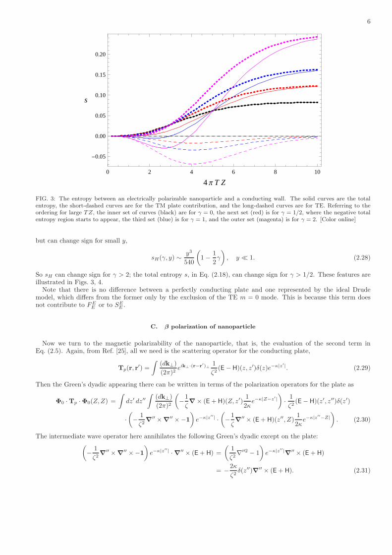
FIG. 3: The entropy between an electrically polarizable nanoparticle and a conducting wall. The solid curves are the totalentropy, the short-dashed curves are for the TM plate contribution, and the long-dashed curves are for TE. Referring to theordering for large TZ, the inner set of curves (black) are for γ = 0, the next set (red) is for γ = 1/2, where the negative totalentropy region starts to appear, the third set (blue) is for γ = 1, and the outer set (magenta) is for γ = 2. [Color online]

but can change sign for small y,

sH(γ, y) ∼y3

540

(

1−1

2γ

)

, y ≪ 1. (2.28)

So sH can change sign for γ > 2; the total entropy s, in Eq. (2.18), can change sign for γ > 1/2. These features areillustrated in Figs. 3, 4.Note that there is no difference between a perfectly conducting plate and one represented by the ideal Drude

model, which differs from the former only by the exclusion of the TE m = 0 mode. This is because this term doesnot contribute to FE

E or to SEE .

C. β polarization of nanoparticle

Now we turn to the magnetic polarizability of the nanoparticle, that is, the evaluation of the second term inEq. (2.5). Again, from Ref. [25], all we need is the scattering operator for the conducting plate,

Tp(r, r′) =

∫

(dk⊥)

(2π)2eik⊥·(r−r

′)⊥1

ζ2(E − H)(z, z′)δ(z)e−κ|z′|. (2.29)

Then the Green’s dyadic appearing there can be written in terms of the polarization operators for the plate as

Φ0 ·Tp ·Φ0(Z,Z) =

∫

dz′ dz′′∫

(dk⊥)

(2π)2

(

−1

ζ∇× (E + H)(Z, z′)

1

2κe−κ|Z−z′|

)

·1

ζ2(E− H)(z′, z′′)δ(z′)

·

(

−1

ζ2∇

′′ ×∇′′ ×−1

)

e−κ|z′′| ·

(

−1

ζ∇

′′ × (E+ H)(z′′, Z)1

2κe−κ|z′′−Z|

)

. (2.30)

The intermediate wave operator here annihilates the following Green’s dyadic except on the plate:(

−1

ζ2∇

′′ ×∇′′ ×−1

)

e−κ|z′′| ·∇′′ × (E+ H) =

(

1

ζ2∇′′2 − 1

)

e−κ|z′′|∇

′′ × (E + H)

= −2κ

ζ2δ(z′′)∇′′ × (E + H). (2.31)

7

0 2 4 6 8 10

-0.2

0.0

0.2

0.4

4 Π T Z

s

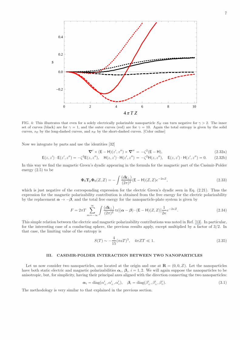
FIG. 4: This illustrates that even for a solely electrically polarizable nanoparticle SH can turn negative for γ > 2. The innerset of curves (black) are for γ = 1, and the outer curves (red) are for γ = 10. Again the total entropy is given by the solidcurves, sE by the long-dashed curves, and sH by the short-dashed curves. [Color online]

Now we integrate by parts and use the identities [32]

∇′ × (E− H)(z′, z′′)×∇

′′ = −ζ2(E− H), (2.32a)

E(z, z′) · E(z′, z′′) = −ζ2E(z, z′′), H(z, z′) · H(z′, z′′) = −ζ2H(z, z′′), E(z, z′) · H(z′, z′′) = 0. (2.32b)

In this way we find the magnetic Green’s dyadic appearing in the formula for the magnetic part of the Casimir-Polderenergy (2.5) to be

Φ0TpΦ0(Z,Z) = −

∫

(dk⊥)

(2π)2(E− H)(Z,Z)e−2κZ , (2.33)

which is just negative of the corresponding expression for the electric Green’s dyadic seen in Eq. (2.21). Thus theexpression for the magnetic polarizability contribution is obtained from the free energy for the electric polarizabilityby the replacement α → −β, and the total free energy for the nanoparticle-plate system is given by

F = 2πT

∞∑

m=−∞

∫

(dk⊥)

(2π)2tr[(α− β) · (E − H)(Z,Z)]

1

2κe−2κZ . (2.34)

This simple relation between the electric and magnetic polarizability contributions was noted in Ref. [13]. In particular,for the interesting case of a conducting sphere, the previous results apply, except multiplied by a factor of 3/2. Inthat case, the limiting value of the entropy is

S(T ) ∼ −4

15(πaT )3, 4πZT ≪ 1. (2.35)

III. CASIMIR-POLDER INTERACTION BETWEEN TWO NANOPARTICLES

Let us now consider two nanoparticles, one located at the origin and one at R = (0, 0, Z). Let the nanoparticleshave both static electric and magnetic polarizabilities αi, βi, i = 1, 2. We will again suppose the nanoparticles to beanisotropic, but, for simplicity, having their principal axes aligned with the direction connecting the two nanoparticles:

αi = diag(αi⊥, α

i⊥, α

iz), βi = diag(βi

⊥, βi⊥, β

iz). (3.1)

The methodology is very similar to that explained in the previous section.

8

0 5 10 15 20

0.00

0.05

0.10

0.15

4 Π T Z

sEE

FIG. 5: The entropy sEE(γ, y) for two anisotropic purely electrically polarizable nanoparticles with separation Z and temper-ature T . When γ = γ1γ2 > 1 the entropy can be negative. The curves, bottom to top for large ZT are for γ = 0 (blue), 1(red), 2 (yellow), respectively. (Color online)

A. Electric polarizability

We start with the interaction between two electrically polarizable nanoparticles. The free energy is

FEE = −T

2

∞∑

m=−∞

tr[4πα1 · Γ0(R) · 4πα2 · Γ0(R)], (3.2)

where the free Green’s dyadic is given in Eq. (2.2). In view of Eq. (2.8), in terms of the polynomials (2.9), a simplecalculation yields (y = 4πZT )

FEE = −23

4πZ7α1zα

2zf(γ, y), (3.3)

normalized to the zero-temperature Casimir-Polder energy [11], where

f(γ, y) =y

23

[

4

(

1− y∂y +1

4y2∂2

y

)

+ 2γ

(

1− y∂y +3

4y2∂2

y −1

4y3∂3

y +1

16y4∂4

y

)]

1

2coth

y

2. (3.4)

Here γ = γ1γ2, where γi = αi⊥/α

iz. The entropy is

SEE =23α1

zα2z

Z6sEE(γ, y), sEE(γ, y) =

∂

∂yf(γ, y). (3.5)

The asymptotic limits are

sEE(γ, y) ∼2 + γ

23, y ≫ 1, (3.6a)

sEE(γ, y) ∼1

2070(1− γ)y3, y ≪ 1, (3.6b)

so even in the pure electric case there is a region of negative entropy for γ > 1. This is illustrated in Fig. 5. Thecoupling of two magnetic polarizabilities is given by precisely the same formulas, except for the replacement α → β.

9

B. EM cross term

For the “interference” term between the magnetic polarization of one nanoparticle and the electric polarization ofthe other, we compute the free energy from the third term in Eq. (2.1),

FEM = −1

2tr[Φ0 · 4πα1 ·Φ0 · 4πβ2] + (1 ↔ 2). (3.7)

This is easily worked out using the following simple form of the Φ0 operator [33]:

Φ0(R) = −ζm

4πZ3R× (1 + ζmZ)e−|ζm|Z , Z = |R|. (3.8)

The result for the free energy is

FEM =7

4πZ7(α1

⊥β2⊥ + β1

⊥α2⊥)g(y), (3.9)

which is normalized to the familiar zero temperature result [14], where

g(y) =y

14

(

y2∂2y − y3∂3

y +1

4y4∂4

y

)

1

2coth

y

2. (3.10)

The entropy is

SEM = −7

Z6(α1

⊥β2⊥ + β1

⊥α2⊥)s

EM , sEM (y) =∂g(y)

∂y. (3.11)

This is always negative, vanishes exponentially fast for large y, and also vanishes rapidly for small y,

sEM ∼ −y5

7056. (3.12)

C. General results

We can present the total entropy for two nanoparticles having both electric and magnetic polarizabilities as follows,

S =1

Z6

[

23α1zα

2zs

EE(γ1αγ

2α, y) + 23β1

zβ2zs

EE(γ1βγ

2β, y)− 7(α1

zβ2zγ

1αγ

2β + β1

zα2zγ

1βγ

2α)s

EM (y)]

, (3.13)

where sEE and sEM are given by Eqs. (3.5) and (3.11), respectively. For small y, the leading behavior of the entropyis

S =y3

90R6[α1

zα2z(1− γ1

αγ2α) + β1

zβ2z(1 − γ1

βγ2β)]

+y5

5040R6[α1

zα2z(4 + 7γ1

αγ2α) + β1

zβ2z(4 + 7γ1

βγ2β) + 5(α1

zβ2zγ

1αγ

2β + β1

zα2zγ

1βγ

2α) +O(y7). (3.14)

In the following six figures we present graphs of the entropy for the case of identical nanoparticles, for simplicity,α1z = α2

z, β1z = β2

z , γ1α = γ2

α, γ1β = γ2

β . In Fig. 6 we show the entropy for isotropic nanoparticles with different ratios

of magnetic to electric polarizabilities; negative entropy appears when the ratio is smaller than about −1/8. This is anonperturbative effect, because the leading power of y3 for small y has a vanishing coefficient in this case, and the y5

term has a positive coefficient —See Eq. (3.14). (The radius of convergence of the series expansions for the free energyis |y| = 2π.) Thus, perfectly conducting spheres, for which the ratio of magnetic to electric polarizabilities is −1/2,exhibit S < 0. In Fig. 7 we examine the case of equal z components of the electric and magnetic polarizabilities, butwhen only the electric polarizability is anisotropic. Negative entropy occurs when γα > 1, which we see perturbativelyfrom Eq. (3.14). In Fig. 8 we consider the nanoparticles as having equal polarizabilities and equal anisotropies.Again, as seen perturbatively, the boundary value for negative entropy is γ = 1. The case of a conducting spherehas β = −α/2. We examine this situation in Fig. 9, for different magnetic anisotropies, and in Fig. 10, for differentelectric anisotropies. In this case the leading term in Eq. (3.14) vanishes at γ = 1, so the appearance of negativeentropy for γ ≤ 1 is nonperturbative. In fact, the boundary values for the two cases are γβ = 0.5436 and γα = 0.7427,respectively. For the latter case, this is illustrated in Fig. 11.An interesting case is the interaction of a perfectly conducting nanoparticle with a Drude nanoparticle, by which

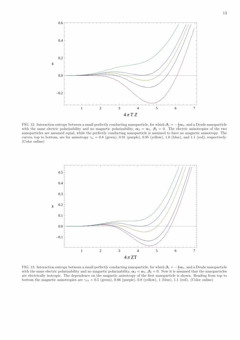
we mean that the latter has vanishing magnetic polarizability. In Fig. 12 we consider the electric anisotropies to bethe same, while in Fig. 13 we show how the entropy changes as we vary the anisotropy of the magnetic polarizabilityof the perfectly conducting sphere. For isotropic spheres there is always a region of negative entropy.

10

5 10 15 20

0

5

10

15

4 Π T Z

s

FIG. 6: Entropy of two identical isotropic nanoparticles (γα = γβ = 1) for different values of the ratio r = β/α. Starting fromhighest to lowest curves on the left, the entropy is given for r = 1 (purple), 0 (green),-1/8 (yellow), -1/2 (red), -2 (blue). Whatis plotted in this and the following figures is s, where the entropy is S = [(α1

z)2/Z6]s. (Color online)

0 2 4 6 8 10

0

5

10

15

4 Π T Z

s

FIG. 7: Here the identical nanoparticles have equal values of αz = βz, and γβ = 1, but different values of the electric anisotropy.Reading from bottom to top on the right, we have γα = 0 (green), 1 (yellow), 2 (red), 4 (blue), respectively. (Color online)

IV. CONCLUSIONS

In this paper we have studied purely geometrical aspects of the entropy that arise from the Casimir-Polder interac-tion, either between a polarizable nanoparticle and a conducting plate, or between two polarizable nanoparticles. Inall cases, the entropy vanishes at T = 0, so the issues mentioned in the Introduction concerning the violation of theNernst heat theorem do not appear in the Casimir-Polder regime. We consider the simplified long distance regime

11

1 2 3 4

-0.5

0.0

0.5

1.0

1.5

2.0

2.5

4 Π T Z

s

FIG. 8: Here the identical nanoparticles have equal electric and magnetic polarizabilities, and equal anisotropies, which, startingfrom the bottom on the right, have the values γ = 0 (green), 1 (yellow), 2 (red), 4 (blue), respectively. (Color online)

0 2 4 6 8 10

-2

-1

0

1

2

3

4 Π T Z

s

FIG. 9: The case of two identical conducting spheres where αz = −2βz, with electrical isotropy, but magnetic anisotropy γβ = 0(yellow), 1 (red), 2 (blue), reading from top to bottom. (Color online)

where we may regard both the electric and magnetic polarizabilities of the nanoparticles as constant in frequency.Thus, throughout we are assuming that the separations Z are large compared to the size of the nanoparticles, a.This same restriction justifies the use of the dipole approximation for the nanoparticles. It has been known for sometime that negative entropy can occur between a purely electrically polarizable isotropic nanoparticle and a perfectlyconducting plate. Here we consider both electric and magnetic polarization for both the nanoparticle and the plate.Negative entropy frequently arises, but requires interplay between electric and magnetic polarizations, or anisotropy,in that the polarizability of the nanoparticles must be different in different directions. Interestingly, although insome cases the negative entropy is already contained in the leading low-temperature expansion of the entropy, in

12

0 2 4 6 8 10

-3

-2

-1

0

1

2

3

4 Π T Z

s

FIG. 10: The case of two identical conducting nanoparticles where αz = −2βz, with magnetic isotropy, but electric anisotropyγα = 0 (blue), 1 (red), 2 (yellow), reading from top to bottom in the middle. (Color online)

1 2 3 4 5 6

-0.4

-0.2

0.0

0.2

0.4

4 Π T Z

s

FIG. 11: Two identical nanoparticles with βz = −αz/2, appropriate for a conducting sphere, isotropic magnetically, but withelectric anisotropies γα = 0.6 (magenta), 0.743 (dashed blue), 0.8 (short dashed red), 1 (black), shown from top to bottom.

other cases negative entropy is a nonperturbative effect, not contained in the leading behavior of the coefficients ofthe low temperature expansion. What we observe here extends what has been found in calculations of the entropybetween a finite sphere and a plate. We summarize our findings in Table I, which, we again emphasize, refer to thedipole approximation, appropriate in the long-distance regime, Z ≫ a. Surprisingly, perhaps, negative entropy is anearly ubiquitous phenomenon: Negative entropy typically occurs when a polarizable nanoparticle is close to anothersuch particle or to a conducting plate. This is not a thermodynamic problem because we are considering only theinteraction entropy, not the total entropy of the system. Nevertheless, it is an intriguing effect, deserving deeperunderstanding.

13

1 2 3 4 5 6 7

-0.2

0.0

0.2

0.4

0.6

4 Π T Z

s

FIG. 12: Interaction entropy between a small perfectly conducting nanoparticle, for which β1 = −

1

2α1, and a Drude nanoparticle

with the same electric polarizability and no magnetic polarizability, α2 = α1, β2 = 0. The electric anisotropies of the twonanoparticles are assumed equal, while the perfectly conducting nanoparticle is assumed to have no magnetic anisotropy. Thecurves, top to bottom, are for anisotropy γα = 0.8 (green), 0.91 (purple), 0.95 (yellow), 1.0 (blue), and 1.1 (red), respectively.(Color online)

1 2 3 4 5 6 7

-0.1

0.0

0.1

0.2

0.3

0.4

0.5

4 Π ZT

s

FIG. 13: Interaction entropy between a small perfectly conducting nanoparticle, for which β1 = −

1

2α1, and a Drude nanoparticle

with the same electric polarizability and no magnetic polarizability, α2 = α1, β2 = 0. Now it is assumed that the nanoparticlesare electrically isotropic. The dependence on the magnetic anisotropy of the first nanoparticle is shown. Reading from top tobottom the magnetic anisotropies are γβ1 = 0.5 (green), 0.66 (purple), 0.8 (yellow), 1 (blue), 1.1 (red). (Color online)

14

Nanoparticle/nanoparticleor nanoparticle/plate Negative entropy?

E/E S < 0 occurs for γα > 1E/M S < 0 alwaysPC/PC S < 0 for γα > 0.74 or γβ > 0.54PC/D S < 0 for γα > 0.91 or γβ > 0.66E/TE plate S < 0 alwaysE/TM plate S < 0 for γα > 2E/PC or D plate S < 0 for γα > 1/2

TABLE I: The table shows when a negative entropy region can occur, in different situations. Here E refers to an electricallypolarizable particle, M a magnetically polarizable particle, PC means a perfectly conducting particle or plate, D means anobject described by the Drude model. TE and TM refer to the transverse electric and transverse magnetic contributions to aperfectly conducting plate. The electric (magnetic) anisotropy is defined by γα = α⊥/αz (γβ = β⊥/βz). Analogous results canbe obtained for other cases by electromagnetic duality.

For confrontation with future experiments, the static approximation for the polarizabilites would have to be removed,a simple task in our general formalism. We are not aware if any present experiments concerning Casimir energiesbetween nanoparticles and surfaces, but we hope this investigation will spur efforts in that direction.

Acknowledgments

KAM and G-LI thank the Laboratoire Kastler Brossel for their hospitality during the period of this work. CNRSand ENS are thanked for their support. KAM’s work was further supported in part by grants from the SimonsFoundation and the Julian Schwinger Foundation.

[1] M. Bostrom and Bo E. Sernelius, Physica A 339, 53 (2004).[2] I. H. Brevik, S. A. Ellingsen and K. A. Milton, New J. Phys. 8, 236 (2006) [quant-ph/0605005].[3] S. A. Ellingsen, Phys. Rev. E 78, 021120 (2008) [arXiv:0710.1015].[4] I. H. Brevik, S. A. Ellingsen, J. S. Høye and K. A. Milton, J. Phys. A 41, 164017 (2008) [arXiv:0710.4882].[5] G. V. Dedkov and A. A. Kyasov, Tech. Phys. Lett. 34, 921 (2008).[6] G.-L. Ingold, A. Lambrecht, and S. Reynaud, Phys. Rev. E 80, 041113 (2009) [arXiv:0905.3608].[7] M. Bordag and I. G. Pirozhenko, Phys. Rev. D 82, 125016 (2010) [arXiv:1010.1217].[8] A. Canaguier-Durand, P. A. M. Neto, A. Lambrecht and S. Reynaud, Phys. Rev. Lett. 104, 040403 (2010)

[arXiv:0911.0913].[9] A. Canaguier-Durand, P. A. Maia Neto, A. Lambrecht, and S. Reynaud, Phys. Rev. A 82, 012511 (2010) [arXiv:1005.4294].

[10] P. Rodriguez-Lopez, Phys. Rev. B 84, 075431 (2011) [arXiv:1104.5447].[11] H. B. G. Casimir and D. Polder, Phys. Rev. 73, 360 (1948).[12] V. B. Bezerra, G. L. Klimchitskaya, V. M. Mostepanenko and C. Romero, Phys. Rev. A 78, 042901 (2008) [arXiv:0809.5229].[13] G. Bimonte, G. L. Klimchitskaya and V. M. Mostepanenko, Phys. Rev. A 79, 042906 (2009) [arXiv:0904.0234].[14] G. Feinberg and J. Sucher, J. Chem. Phys. 48, 3333 (1968).[15] A. B. McLachlan, Proc. R. Soc. London, Ser. A 271, 387 (1963).[16] A. B. McLachlan, Proc. R. Soc. London, Ser. A 274, 80 (1963).[17] G. Barton, Phys. Rev. A 64, 032102 (2001).[18] H. Haakh, F. Intravaia, C. Henkel, S. Spagnolo, R. Passante, B. Power, and F. Sols, Phys. Rev. A 80, 062905 (2009).[19] D. P. Craig and E. A. Power, Chem. Phys. Lett. 3, 195 (1969).[20] D. P. Craig and E. A. Power, Int. J. Quantum Chem. 3, 903 (1969).[21] T. Emig, R. L. Jaffe, M. Kardar, and A. Scardicchio, Phys. Rev. Lett. 96, 080403 (2006) [cond-mat/0601055].[22] T. Emig, R. L. Jaffe, M. Kardar, and A. Scardicchio, Phys. Rev. Lett. 99, 170403 (2007) [arXiv:0707.1862].[23] C. E. Roman-Valazquez and Bo E. Sernelius, J. Phys. A 41, 164008 (2008); arXiv:0806.2067.[24] C. E. Roman-Valazquez and Bo E. Sernelius, Phys. Rev. A 78, 032111 (2008) [arXiv:0807.1626].[25] K. A. Milton, E. K. Abalo, P. Parashar, N. Pourtolami, I. Brevik, S. A. Ellingsen, S. Y. Buhmann, and S. Scheel, “Casimir-

Polder repulsion: Three-body effects,” paper in preparation.[26] C. Noguez, C. E. Roman-Velazquez, R. Esquivel-Sirvent, and C. Villarreal, Europhys. Lett. 67, 191 (2004) [quant-

ph/0310068].

15

[27] C. Noguez and C. E. Roman-Velazguez, Phys. Rev. B 70, 195412 (2004) [quant-ph/0312009].[28] K. A. Milton, P. Parashar, J. Wagner, and I. Cavero-Pelaez, J. Vac. Sci. Technol. B 28, C4A8–C4A16 (2010).[29] H. Levine and J. Schwinger, Comm. Pure Appl. Math. III 4, 355 (1950), reprinted in K. A. Milton and J. Schwinger,

Electromagnetic Radiation: Variational Methods, Waveguides, and Accelerators (Springer, Berlin, 2006), p. 543.[30] K. A. Milton, P. Parashar and J. Wagner, in The Casimir effect and cosmology, ed. S. D. Odintsov, E. Elizalde, and O. B.

Gorbunova, in honor of Iver Brevik (Tomsk State Pedagogical University) pp. 107-116 (2009) [arXiv:0811.0128].[31] T. Matsubara, Prog. Theor. Phys. 14, 351 (1955).[32] K. A. Milton, P. Parashar, E. K. Abalo, F. Kheirandish and K. Kirsten, Phys. Rev. D 88, 045030 (2013) [arXiv:1307.2535].[33] K. A. Milton, P. Parashar, N. Pourtolami and I. Brevik, Phys. Rev. D 85, 025008 (2012) [arXiv:1111.4224].[34] K. A. Milton, J. Wagner, P. Parashar and I. Brevik, Phys. Rev. D 81, 065007 (2010) [arXiv:1001.4163].