Near-Real-Time Simulation and Internet-Based

Near-Real-Time Simulation and Internet-BasedDelivery of Forecast-Flood Inundation MapsUsing Two-Dimensional Hydraulic Modeling:A Pilot Study of the Snoqualmie River, Washington

U.S. GEOLOGICAL SURVEYWater-Resources Investigations Report 02-4251

Near-Real-Time Simulation and Internet-Based Delivery of Forecast-Flood Inundation Maps Using Two-Dimensional Hydraulic Modeling: A Pilot Study of the Snoqualmie River, Washington

By J.L. Jones, J.M. Fulford, and F.D. Voss

U.S. GEOLOGICAL SURVEY

Water-Resources Investigations Report 02-4251

Tacoma, Washington2002

U.S. DEPARTMENT OF THE INTERIOR
GALE A. NORTON, Secretary
U.S. GEOLOGICAL SURVEY
Charles G. Groat, Director
Any use of trade, product, or firm names in this publication is for descriptive purposes only and does not imply endorsement by the U.S. Government.

For additional information write to:

Director, Washington Water Science CenterU.S. Geological Survey1201 Pacific Avenue – Suite 600Tacoma, Washington 98402http://wa.water.usgs.gov

Copies of this report can be purchased from:

U.S. Geological SurveyInformation ServicesBuilding 810Box 25286, Federal CenterDenver, CO 80225-0286

http://wa.water.usgs.gov

Contents iii

CONTENTSAbstract ................................................................................................................................................................ 1Introduction .......................................................................................................................................................... 1

Need for Forecast Flood Maps.................................................................................................................... 2New Technologies Make It Possible........................................................................................................... 2

Elevation Data.................................................................................................................................... 2Hydraulic Modeling ........................................................................................................................... 3Geographic Information Systems and Internet Map Servers ............................................................. 3

Purpose and Scope ...................................................................................................................................... 3Two-Dimensional Simulation of Flood Inundation for the Snoqualmie River, Washington .............................. 4

Selection and Characteristics of Hydraulic Model...................................................................................... 4Model Construction and Boundary Conditions........................................................................................... 4Model Calibration, Verification, and Testing ............................................................................................. 5Application to Flood Forecasts ................................................................................................................... 10Forecast-Flood Simulation Results ............................................................................................................. 12

Automated Processing and Display of Forecast-Flood Information.................................................................... 17File-Processing Program Interface.............................................................................................................. 17Creating TrimR2D Input File From National Weather Service River Forecast Center Forecast Data....... 17Converting TrimR2D Output to Shape Files .............................................................................................. 19

Internet Map Server Development ....................................................................................................................... 19Summary .............................................................................................................................................................. 20References ............................................................................................................................................................ 21Appendix A. File Processing Programs and Model Input Example File ............................................................ 22

iv Figures

FIGURES

Figure 1. Map showing location of study reach and computational domain of the hydraulic model of the Snoqualmie River, Washington, showing model grid and U.S. Geological Survey stream-gaging stations ....................................................................................................................... 6

Figure 2. Hydrographs for the flood event of November 24, 1986, on the study reach of the Snoqualmie River, Washington ......................................................................................................... 7

Figure 3. Contour plot showing simulated peak water-surface elevations for the flood event of November 24, 1986, on the study reach of the Snoqualmie River, Washington, for a Manning’s roughness value of 0.12 ................................................................................................... 8

Figure 4. Hydrographs for the flood event of December 3, 1975, on the study reach of the Snoqualmie River, Washington ......................................................................................................... 9

Figure 5. Contour plot showing simulated peak water-surface elevations for the flood event of December 3, 1975, on the study reach of the Snoqualmie River, Washington, for a Manning’s roughness value of 0.12 ................................................................................................... 11

Figure 6. Contour plots showing time from start of simulation (November 23, 1986, 1:00 a.m.) to arrival of floodwater for the study reach of the Snoqualmie River, Washington, for the flood event of November 24, 1986......................................................................................... 13

Figure 7. Contour plot showing time from start of simulation (November 23, 1986, 1:00 a.m.) to arrival of flood peak for the study reach of the Snoqualmie River, Washington, for the flood event of November 24, 1986.........................................................................................14

Figure 8. Contour plot showing time from start of simulation (December 1, 1975, 1:00 a.m.) to arrival of floodwater for the study reach of the Snoqualmie River, Washington, for the flood event of December 3, 1975 ...........................................................................................15

Figure 9. Contour plot showing time from start of simulation (December 1, 1975, 1:00 a.m.) to arrival of flood peak for the study reach of the Snoqualmie River, Washington, for the flood event of December 3, 1975 ........................................................................................... 16

Figure 10. Screen capture showing user interface for the file-processing program, written in Visual Basic ..... 17

Tables v

TABLES

Table 1. Match between measured and computed peak water-surface elevations for calibration of the Snoqualmie River model, using the flood event of November 24, 1986, and a Manning’s roughness value of 0.12 ................................................................................................... 9

Table 2. Match between measured and computed peak water-surface elevations for verification of the Snoqualmie River model, using the flood event of December 3, 1975, and a Manning’s roughness value of 0.12 ..................................................................................................................... 12

Table 3. Type, purpose, source, and use of files used in the file-processing program .................................... 18

vi Conversion Factors and Datums

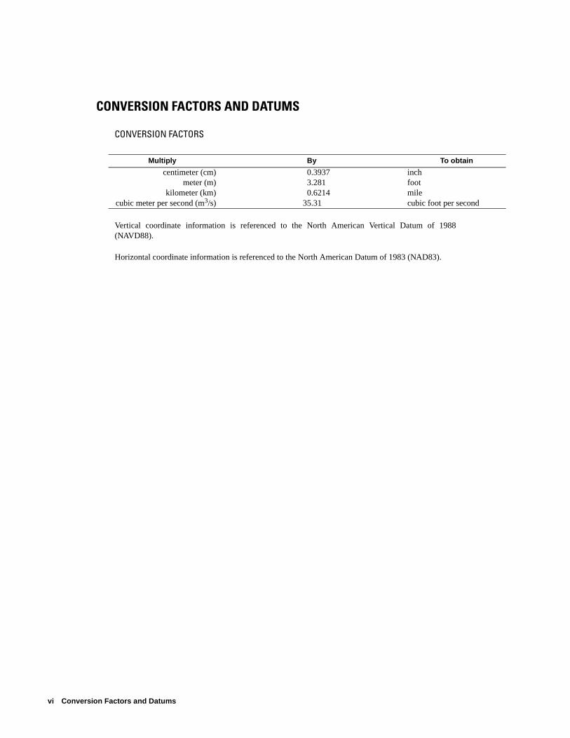
CONVERSION FACTORS AND DATUMS

CONVERSION FACTORS

Vertical coordinate information is referenced to the North American Vertical Datum of 1988 (NAVD88).

Horizontal coordinate information is referenced to the North American Datum of 1983 (NAD83).

Multiply By To obtain

centimeter (cm) 0.3937 inchmeter (m) 3.281 foot

kilometer (km) 0.6214 milecubic meter per second (m3/s) 35.31 cubic foot per second

Near-Real-Time Simulation and Internet-Based Delivery of Forecast-Flood Inundation Maps Using Two-Dimensional Hydraulic Modeling: A Pilot Study for the Snoqualmie River, Washington

By J.L. Jones, J.M. Fulford, and F.D. Voss

ABSTRACT

A system of numerical hydraulic modeling, geographic information system processing, and Internet map serving, supported by new data sources and application automation, was developed that generates inundation maps for forecast floods in near real time and makes them available through the Internet. Forecasts for flooding are generated by the National Weather Service (NWS) River Forecast Center (RFC); these forecasts are retrieved automatically by the system and prepared for input to a hydraulic model. The model, TrimR2D, is a new, robust, two-dimensional model capable of simulating wide varieties of discharge hydrographs and relatively long stream reaches. TrimR2D was calibrated for a 28-kilometer reach of the Snoqualmie River in Washington State, and is used to estimate flood extent, depth, arrival time, and peak time for the RFC forecast. The results of the model are processed automatically by a Geographic Information System (GIS) into maps of flood extent, depth, and arrival and peak times. These maps subsequently are processed into formats acceptable by an Internet map server (IMS). The IMS application is a user-friendly interface to access the maps over the Internet; it allows users to select what information they wish to see presented and allows the authors to define scale-dependent availability of map layers and their symbology (appearance of map features). For example, the IMS presents a background of a

digital USGS 1:100,000-scale quadrangle at smaller scales, and automatically switches to an ortho-rectified aerial photograph (a digital photograph that has camera angle and tilt distortions removed) at larger scales so viewers can see ground features that help them identify their area of interest more effectively. For the user, the option exists to select either background at any scale. Similar options are provided for both the map creator and the viewer for the various flood maps. This combination of a robust model, emerging IMS software, and application interface programming should allow the technology developed in the pilot study to be applied to other river systems where NWS forecasts are provided routinely.

INTRODUCTION

Existing flood forecasts are limited to stage (water-surface height) or flow predictions only for specific flow forecast points, and provide no predictions for area or depth of inundation. New developments in technology and software allowed the U.S. Geological Survey (USGS) to develop a method to generate information previously not available but greatly desired by flood-response officials – a flood forecast map. The USGS combined new data sources, new computational techniques, and new map creation and delivery software systems to pilot near-real-time mapping of forecast or imminent flooding as part of its Urban Geologic and Hydrologic Natural Hazards Initiative. This multidisciplinary study of natural

Introduction 1

hazards is referred to locally as the Seattle Area Natural Hazards Project. The new mapping method was demonstrated in a pilot study for a reach of the Snoqualmie River in Washington State. New data sources provide high-accuracy, areally dense elevation data; new computational techniques provide a robust and stable two-dimensional hydraulic model capable of simulating a wide range of flooding situations on longer river reaches than were previously possible; and new software systems allow the post-processing of simulations into flood inundation and depth maps that can be delivered over the Internet in a flexible and user-friendly way.

Need for Forecast Flood Maps

For the most part, the only flood maps available for an area are maps prepared for the Federal Emergency Management Agency's (FEMA) National Flood Insurance Program (NFIP). These Flood Insurance Rate Maps (FIRMs) originally were intended to identify where property owners were required to purchase Federal flood insurance in order to be eligible for disaster assistance in the event of flooding. A community or county that participates in the NFIP agrees to abide by certain regulations, such as not allowing construction in the most flood-prone areas, in return for a promise of federal assistance to cope with the aftermath of a major flood. Because these maps often were the only source of information about flooding potential, they typically were also used for all manner of flood planning and mitigation and any zoning regulations the county or community chose to enact. FIRMs delineate potential flood inundation areas for floods of selected recurrence intervals (probabilities) only, and do not include water depth information.

The theoretical flood flows used to make FIRMs are determined statistically – for example, the flow that has a 1-percent chance of occurring on that stream in the immediate vicinity of the area to be mapped (determined from streamflow data where available, and otherwise estimated from nearby streams that do have streamflow data). This 1-percent-chance flood is commonly referred to as the "100-year" flood, though it is more appropriately conceived of as a "design flood" – a baseline used for planning, design, and regulation. The more common term has led to some confusion regarding the actual probability of major

flooding in a region; because an area such as the Pacific Northwest has many streams, the actual probability of occurrence of "100-year" floods somewhere in the region has been estimated to be more on the order of one every 2 to 3 years (Brent Troutman, U.S. Geological Survey, written commun., 2001).

The National Weather Service's (NWS) River Forecast Centers (RFCs) currently forecast flows and flood stage (height of water) at forecast points (typically a USGS stream-gaging station), but not for areas between forecast points. They do not make any maps depicting inundated areas at or between forecast points. RFC forecasts are issued whenever precipitation forecasts indicate that flooding is likely; these forecasts are generated daily and comprise predictions at 6-hour increments spanning 3 to 5 days. Information about flood extent and depth for a storm-specific flood would aid emergency response officials in identifying the areas where their resources are needed the most immediately or the most critically.

New Technologies Make It Possible

Newly available ground-elevation data, a new robust and stable two-dimensional hydraulic flow model, relatively new Geographic Information System (GIS) technology, and Internet map-serving software make near-real-time mapping and delivery of forecast-flood inundation by the Internet feasible.

Elevation Data

Until recently, elevation data of adequate accuracy to use in hydraulic flow models were prohibitively expensive to obtain and process, and were gathered for selected stream-channel and flood plain cross sections only. This is one reason one-dimensional hydraulic models have predominated in the past. Now, very-high-accuracy elevation data (accurate to 15 cm, or around one-half foot) are relatively affordable, especially considering the variety of applications for which they are suited.

LIght Detection and Ranging (LIDAR) technology recently has moved from a research application to a practical application for collecting very-high-accuracy elevation data. Typically, these data are collected from a plane flying a few thousand feet above the land surface. The sensor is essentially a sophisticated laser rangefinder that scans a swath

2 Near-Real-Time Simulation and Internet-Based Delivery of Two-Dimensional Forecast-Flood Maps: A Pilot Study of the Snoqualmie River, WA

beneath the plane with tens of thousands of infrared light pulses per second. The plane's location and orientation are determined with kinematic differential geographic positioning systems (KDGPS) and inertial navigation units, respectively. Determining ground elevations is, in concept, a simple process of geometrically adjusting each raw laser-ranged distance using the plane's absolute position, the scan angle of the pulse, and the pitch, yaw, and roll of the aircraft at the instant the pulse was emitted. Processing such large data streams with the accuracy and precision required to achieve very-high-accuracy land elevations is nevertheless an impressive feat, and even after that is accomplished, a large percentage of the data points have reflected off of trees, buildings, bridges, and other features. Numerous methods have been devised for filtering out elevation data points not desired in a hydraulic model (such as elevations of tree tops or bridges), and generally the methods are proprietary and under continual refinement. Precise specifications should be provided for the collection and processing of LIDAR data for use in hydraulic models, and the adequacy of the data for use in the model should be assessed carefully.

Hydraulic Modeling

For many years, one-dimensional models were the only type of hydraulic flow model readily available, and they remain the most common method of simulating flood flows.

One reason one-dimensional models remain prevalent is because existing two-dimensional models, such as the U.S. Army Corps of Engineers (COE) RMA2 or the USGS FESWMS, are limited by the robustness of the algorithms used to solve the governing equations. These limitations include the length of the reach through which flow is simulated and characteristics of the hydrograph to be simulated (such as no extreme, sudden flow changes). In addition, the numerical stability of most current two-dimensional models often requires careful preparation of a unique set of initial conditions that will allow the model to simulate the desired hydrograph successfully; this may require repetitive simulations that gradually evolve into

the initial conditions needed. The model used in this mapping pilot is TrimR2D, which, because of a unique solution method, allows simulation of flows through long reaches, can solve hydrographs of rapidly changing flows, and is adequately robust to handle an input hydrograph without tedious trial-and-error preparation of initial conditions (J.M. Fulford, U.S. Geological Survey, written commun., 2002).

Geographic Information Systems and Internet Map Servers

Geographic Information System software (in this pilot, ArcInfo© by ESRI) software is used to process simulation results to produce maps showing flood extent and depth. These maps are further processed into a format compatible with the Internet map server software (IMS; in this pilot, MapGuide© by AutoDesk). IMS software is a relatively new technology that allows the map user greater control over what is seen and the scale at which it is seen. Finally, all of the required pieces—forecast acquisition, flow modeling, map generation, and map presentation—are automated using Visual Basic, one of the most widely-used programming languages.

Purpose and Scope

This report describes the data, software, and methodology used to generate and provide on the Internet forecast-flood maps in near real time, and the application of the system to a reach of the Snoqualmie River, Washington. The report (1) documents the calibration and verification of TrimR2D for the study reach of the Snoqualmie River and the simulation of flood inundation for the reach; and (2) describes the automated processing and display of the forecast-flood inundation simulation. The discussion of automation includes processing of the model output into flood-extent and -depth maps with a GIS; processing of the maps for the Internet map server; Internet map server authoring; and automation of the entire process using Visual Basic. The report provides sufficient detail for subsequent investigators to duplicate and(or) improve on the methodology.

Introduction 3

TWO-DIMENSIONAL SIMULATION OF FLOOD INUNDATION FOR THE SNOQUALMIE RIVER, WASHINGTON

A 28-kilometer reach of the Snoqualmie River east of Seattle, Washington, was selected for the pilot study because it satisfied a variety of needs of the multidisciplinary Seattle Area Natural Hazards Project team. The team needed a study area where detailed elevation data could be collected for geologic mapping, for locating evidence of tectonic faulting at the land surface, for flood mapping, and for geomorphic analyses of channel migration. The Snoqualmie River was selected because the undetermined eastern end of the Seattle Fault zone is anticipated to be somewhere between Seattle and Snoqualmie, because the Snoqualmie River is proximal to rapidly growing Seattle suburbs, and because the river is highly sinuous, with both complex overbank flow patterns and the possibility of channel migration and avulsion – features that make simulation of flooding in this system very challenging.

The recent emergence of LIDAR as an affordable method of quickly collecting very-high-accuracy areally dense elevation data over large areas stands to greatly improve the quality and detail of floodplain analyses, particularly flood inundation mapping (Jones, 2001). Basin delineation, stream delineation, channel migration analyses, and flow modeling will likely be improved from applications of this technology. Because there are numerous other uses for such data, many counties and cities across the Nation are acquiring these data. Characteristics of raw LIDAR data sets vary from contractor to contractor because of differences in equipment and collection methods. The data used for this model had an areal density of approximately one data point per square meter and a vertical accuracy of approximately 15 cm. These values vary somewhat as a function of the scan angle of the airborne sensor, the most dense and accurate data being those collected at nadir – directly beneath the sensor. The data were verified by surveyed ground control points in the pilot study area. The processing of raw LIDAR data typically is complex and generally should be done by the LIDAR provider, with carefully determined specifications and quality assurance by the

customer. The details of LIDAR data collection and processing are beyond the scope of this report, and for the ensuing discussion it is assumed that the LIDAR provider has processed the data to a raster (on the order of a few meters spacing) representation of bare-ground elevations.

To prepare for near-real-time simulation of forecast-flood inundation, a hydraulic model must be selected, constructed, calibrated, and verified. The selected model must be appropriate for the conditions to be simulated, including the geometry of the flow system and the flows to be simulated. Subsequently, the model grid must be constructed, model boundary conditions must be specified, and model parameters must be calibrated and verified using a set of stage-discharge observations for a flow similar to those to be simulated. The resulting calibrated and verified model can be applied to flow scenarios that are within the range of flows for which the calibration and verification are valid.

Selection and Characteristics of Hydraulic Model

Because of the ambitious project goals, a robust computational flow model was required to provide areal flood inundation information. The TrimR2D model was selected as an appropriate model for inundation simulations. The model has been used to simulate flows in a river system (Ostenaa and others, 1999) and is based extensively on the Trim estuarine model (Casulli, 1990, Cheng and others, 1993). The TrimR2D model solves the shallow-water flow equations (Albertson, 1960) using a semi-implicit, semi-Lagrangian finite-difference numerical scheme (Staniforth and Cote, 1991). Finite-difference schemes subdivide the model area into a discrete number of nodes and solve the flow equations at each node. The TrimR2D model is capable of handling large local changes in water-surface elevation and velocity and does not fail or become terminally unstable as model cells change from active (wet) to inactive (dry) during the course of the simulation. The numerical scheme and model operation of TrimR2D are documented by Fulford (J.M. Fulford, U.S. Geological Survey, written commun., 2002).


Model Construction and Boundary Conditions

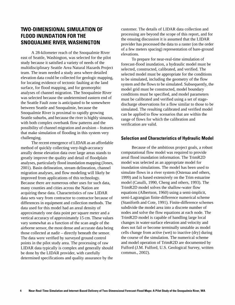
Model construction for TrimR2D included developing a two-dimensional computational grid of ground-surface elevations for the area of interest, specifying upstream and downstream hydraulic boundary conditions, and selecting an appropriate computational time step for simulations. The model was applied to a reach of the Snoqualmie River that is between USGS stream-gaging stations near Snoqualmie Falls and Carnation, Wash. (fig. 1). The model area includes a 28-kilometer length of the Snoqualmie River and portions of the Raging and Tolt Rivers, and covers an area that is 13,200 m by 8,240 m. The 8-meter horizontal-resolution topography grid constructed for the model was resampled directly from the 2-meter-resolution LIDAR elevation data. However, because the model solves for elevations at every other grid cell, and for velocities at the intervening cells, the effective horizontal resolution of the flow model is 16 m. Flow is computed by the TrimR2D application over a 515-by-825 node grid. Nodes above an elevation of 45 m are set inactive (fig. 1). The flow variables simulated include flow depth and the x and y horizontal velocities.

The TrimR2D model requires specification of a time series of discharge at all points of surface-water inflow to the model area as upstream boundary conditions, and of water-surface elevation at all points of surface-water outflow from the model area as downstream boundary conditions. The Snoqualmie River model uses observed discharges at USGS stream-gaging station Raging River near Fall City (12145500), Tolt River near Carnation (12148500), and Snoqualmie River near Snoqualmie (12144500) as upstream boundary conditions (fig. 1), conceptually, the inflow of water into the model domain. Hourly observed water-surface elevation at the Snoqualmie River near Carnation gage (12149000) was used as the downstream boundary condition (fig. 1).

The computational time-step size for the Snoqualmie River model was set to 1.5 seconds. That time-step size allowed the model to propagate the flow across dry areas while maintaining model stability for the flow events tested. The model linearly interpolates inflow discharges and outflow water-surface data from a larger time interval (1 hour) to the smaller computational time step.

The model was run on a 1998-vintage personal computer for this pilot.

Model Calibration, Verification, and Testing

The implementation of the TrimR2D model required calibration and verification of the roughness values (Manning's roughness coefficients) for the Snoqualmie model. Two flow events were used to calibrate and verify the model: the flood events of November 24, 1986, and December 3, 1975. The flow model was calibrated by adjusting roughness coefficients until computed peak water-surface elevations reasonably matched measured peak water elevations for the 1986 flood event. The application subsequently was verified by comparing computed and measured peak water elevations for the 1975 flood event. Inflow discharges and outflow water-surface elevations were available at a 1-hour time interval for both events. Measured high-water marks were available for both floods at five stations from the COE (Dennis Mekkers, U.S. Army Corps of Engineers, written comm., 2001), but data were not available for comparing simulated and actual inundated areas.

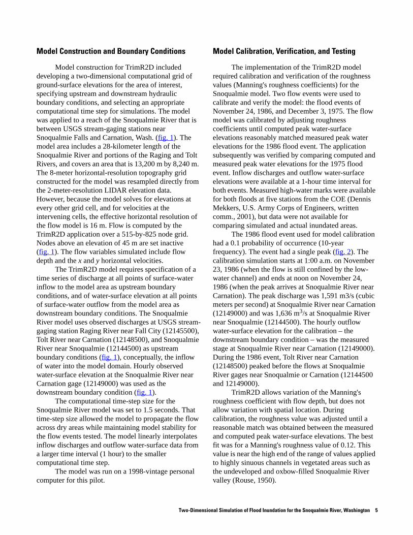
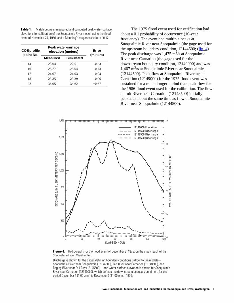
The 1986 flood event used for model calibration had a 0.1 probability of occurrence (10-year frequency). The event had a single peak (fig. 2). The calibration simulation starts at 1:00 a.m. on November 23, 1986 (when the flow is still confined by the low-water channel) and ends at noon on November 24, 1986 (when the peak arrives at Snoqualmie River near Carnation). The peak discharge was 1,591 m3/s (cubic meters per second) at Snoqualmie River near Carnation (12149000) and was 1,636 m3/s at Snoqualmie River near Snoqualmie (12144500). The hourly outflow water-surface elevation for the calibration – the downstream boundary condition – was the measured stage at Snoqualmie River near Carnation (12149000). During the 1986 event, Tolt River near Carnation (12148500) peaked before the flows at Snoqualmie River gages near Snoqualmie or Carnation (12144500 and 12149000).

TrimR2D allows variation of the Manning's roughness coefficient with flow depth, but does not allow variation with spatial location. During calibration, the roughness value was adjusted until a reasonable match was obtained between the measured and computed peak water-surface elevations. The best fit was for a Manning's roughness value of 0.12. This value is near the high end of the range of values applied to highly sinuous channels in vegetated areas such as the undeveloped and oxbow-filled Snoqualmie River valley (Rouse, 1950).

Two-Dimensional Simulation of Flood Inundation for the Snoqualmie River, Washington 5

6 Nea

POWERLINE

Rive

r

Fall City

Carnation

Snoqualmie

Tolt

Rive

r

River

12148000

12147500

12149000

1214450012145500

12148500

Ragi

ng

0

0

1 2 3 4

4

5 KILOMETERS

1 2 3 5 MILES

Base from U.S. Geological Survey,Digital Raster Graphic, 1:100 000, 1975,Universal Transverse Mercator, Zone 10

EXPLANATION

12148000

COMPUTATIONAL DOMAIN OF HYDRAULIC MODEL

SNOQUALMIE RIVER

MODEL GRID IN INCREMENTS OF TWO HUNDRED 8-METER CELLS

U.S. GEOLOGICAL SURVEY STREAM-GAGING STATION AND NUMBER

LOCATION OF INFLOW TO MODEL

WASHINGTON

Study site

T26N

T25N

T24N

T23NR7E R8E R9E

Figure 1. Location of study reach and computational domain of the hydraulic model of the Snoqualmie River, Washington, showing model grid and U.S. Geological Survey stream-gaging stations.

r-Real-Time Simulation and Internet-Based Delivery of Two-Dimensional Forecast-Flood Maps: A Pilot Study of the Snoqualmie River, WA

12149000 Elevation12144500 Discharge12148500 Discharge12145500 Discharge

1,750

1,500

1,250

1,000

750

500

250

00 20 40 6010 30 50 70

DIS

CHA

RGE,

IN C

UB

IC M

ETER

S PE

R SE

CON

D

ELAPSED HOUR

15

16

17

18

19

14

WAT

ER-S

URF

ACE

ELE

VATI

ON

, IN

MET

ERS

Figure 2. Hydrographs for the flood event of November 24, 1986, on the study reach of the Snoqualmie River, Washington. Water-surface elevation is shown for stream-gaging station Snoqualmie River near Carnation (12149000) and discharge is shown for stations Snoqualmie River near Snoqualmie (12144500), Tolt River near Carnation (12148500), and Raging River near Fall City (12145500) for the period November 23 (1:00 a.m.) to November 25 (11:00 p.m.), 1986.

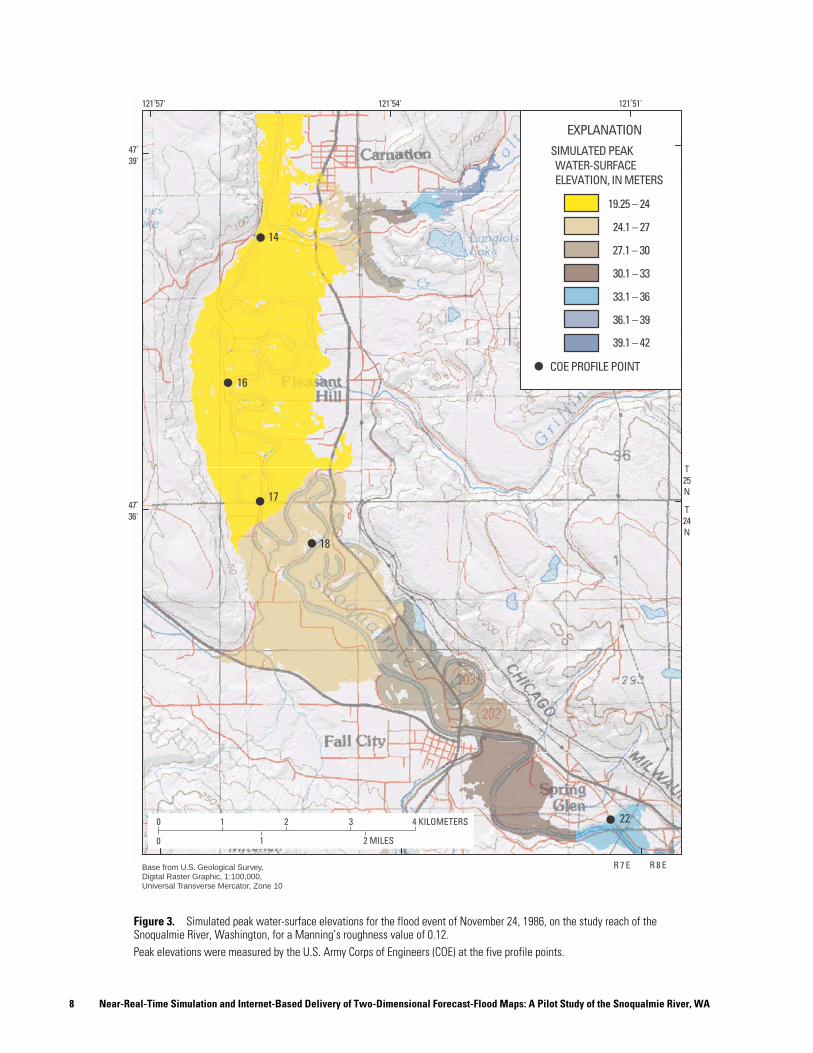
Simulated peak water-surface elevations computed by the Snoqualmie River model for the 70-hour calibration hydrograph are shown in figure 3. Peak water-surface elevations were determined by selecting from the hourly model output the maximum elevation determined at each node over the simulation. Computed peak water-surface elevations were compared with peak elevations measured by the COE for the flood at the five profile points located in the

modeled reach (fig. 3). Table 1 lists the measured and computed water-surface elevations for the five COE points. Errors for the computed water elevations varied from -0.73 m to +0.67 m. Water-surface elevation was overestimated by the model at the most upstream observation point and was underestimated at the downstream observation points. The average error was -0.14 m and the average absolute error was 0.41 m for the COE observation points.


8 Nea

EXPLANATIONSIMULATED PEAK WATER-SURFACE ELEVATION, IN METERS

COE PROFILE POINT

19.25 – 24

24.1 – 27

27.1 – 30

30.1 – 33

33.1 – 36

36.1 – 39

39.1 – 42

0

0

1 2 3 4 KILOMETERS

1 2 MILES

121˚57' 121˚54' 121˚51'

47˚39'

47˚36'

T25N

T24N

R 7 E R 8 EBase from U.S. Geological Survey,Digital Raster Graphic, 1:100,000, Universal Transverse Mercator, Zone 10

14

16

17

18

22

r-

Figure 3. Simulated peak water-surface elevations for the flood event of November 24, 1986, on the study reach of the Snoqualmie River, Washington, for a Manning’s roughness value of 0.12. Peak elevations were measured by the U.S. Army Corps of Engineers (COE) at the five profile points.

Real-Time Simulation and Internet-Based Delivery of Two-Dimensional Forecast-Flood Maps: A Pilot Study of the Snoqualmie River, WA

. The 1975 flood event used for verification had about a 0.1 probability of occurrence (10-year frequency). The event had multiple peaks at Snoqualmie River near Snoqualmie (the gage used for the upstream boundary condition, 12144500; (fig. 4). The peak discharge was 1,475 m3/s at Snoqualmie River near Carnation (the gage used for the downstream boundary condition, 12149000) and was 1,467 m3/s at Snoqualmie River near Snoqualmie (12144500). Peak flow at Snoqualmie River near Carnation (12149000) for the 1975 flood event was sustained for a much longer period than peak flow for the 1986 flood event used for the calibration. The flow at Tolt River near Carnation (12148500) initially peaked at about the same time as flow at Snoqualmie River near Snoqualmie (12144500).

Table 1. Match between measured and computed peak water-surface elevations for calibration of the Snoqualmie River model, using the flood event of November 24, 1986, and a Manning’s roughness value of 0.12

COE profile point No.

Peak water-surface elevation (meters) Error

(meters)Measured Simulated

14 23.04 22.51 -0.53

16 23.77 23.04 -0.73

17 24.07 24.03 -0.04

18 25.35 25.29 -0.06

22 33.95 34.62 +0.67

12149000 Elevation12144500 Discharge12148500 Discharge12145500 Discharge

1,750

1,500

1,250

1,000

750

500

250

00 20 40 60 80 100 120

DIS

CHA

RGE,

IN C

UB

IC M

ETER

S PE

R SE

CON

D

ELAPSED HOUR

15

16

17

18

19

14

WAT

ER-S

URF

ACE

ELE

VATI

ON

, IN

MET

ERS

Figure 4. Hydrographs for the flood event of December 3, 1975, on the study reach of the Snoqualmie River, Washington. Discharge is shown for the gages defining boundary conditions (inflow to the model)—Snoqualmie River near Snoqualmie (12144500), Tolt River near Carnation (12148500), and Raging River near Fall City (12145500)—and water-surface elevation is shown for Snoqualmie River near Carnation (12149000), which defines the downstream boundary condition, for the period December 1 (1:00 a.m.) to December 6 (11:00 p.m.), 1975.


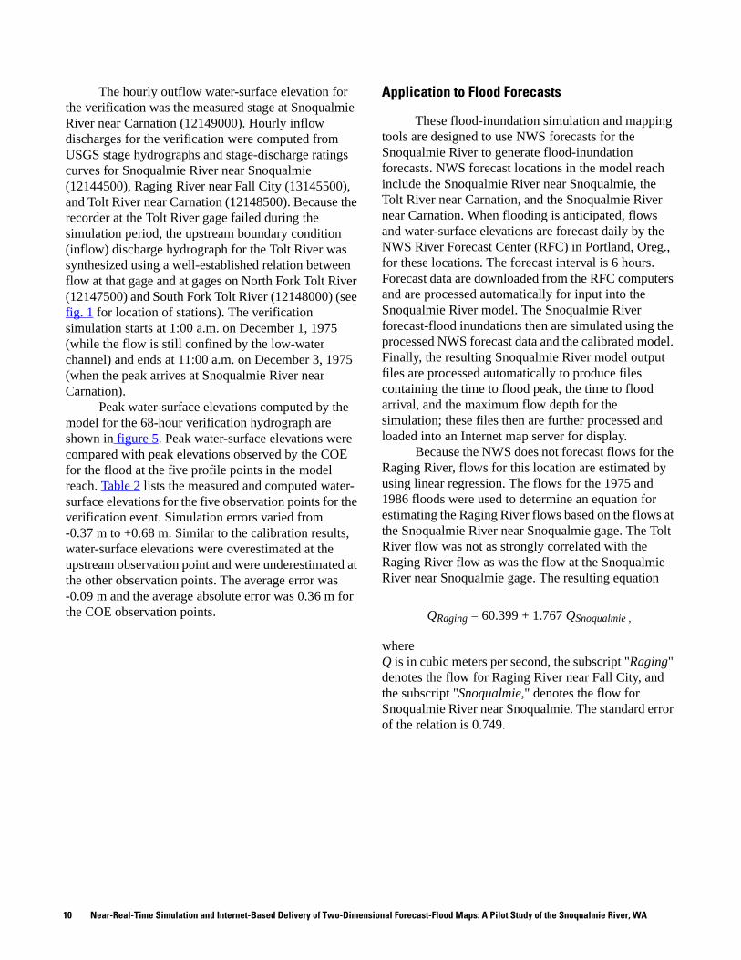
The hourly outflow water-surface elevation for the verification was the measured stage at Snoqualmie River near Carnation (12149000). Hourly inflow discharges for the verification were computed from USGS stage hydrographs and stage-discharge ratings curves for Snoqualmie River near Snoqualmie (12144500), Raging River near Fall City (13145500), and Tolt River near Carnation (12148500). Because the recorder at the Tolt River gage failed during the simulation period, the upstream boundary condition (inflow) discharge hydrograph for the Tolt River was synthesized using a well-established relation between flow at that gage and at gages on North Fork Tolt River (12147500) and South Fork Tolt River (12148000) (see fig. 1 for location of stations). The verification simulation starts at 1:00 a.m. on December 1, 1975 (while the flow is still confined by the low-water channel) and ends at 11:00 a.m. on December 3, 1975 (when the peak arrives at Snoqualmie River near Carnation).

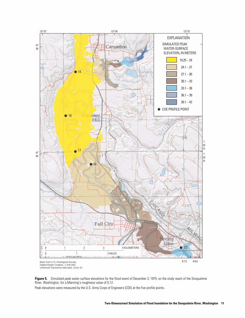
Peak water-surface elevations computed by the model for the 68-hour verification hydrograph are shown in figure 5. Peak water-surface elevations were compared with peak elevations observed by the COE for the flood at the five profile points in the model reach. Table 2 lists the measured and computed water-surface elevations for the five observation points for the verification event. Simulation errors varied from -0.37 m to +0.68 m. Similar to the calibration results, water-surface elevations were overestimated at the upstream observation point and were underestimated at the other observation points. The average error was -0.09 m and the average absolute error was 0.36 m for the COE observation points.

Application to Flood Forecasts

These flood-inundation simulation and mapping tools are designed to use NWS forecasts for the Snoqualmie River to generate flood-inundation forecasts. NWS forecast locations in the model reach include the Snoqualmie River near Snoqualmie, the Tolt River near Carnation, and the Snoqualmie River near Carnation. When flooding is anticipated, flows and water-surface elevations are forecast daily by the NWS River Forecast Center (RFC) in Portland, Oreg., for these locations. The forecast interval is 6 hours. Forecast data are downloaded from the RFC computers and are processed automatically for input into the Snoqualmie River model. The Snoqualmie River forecast-flood inundations then are simulated using the processed NWS forecast data and the calibrated model. Finally, the resulting Snoqualmie River model output files are processed automatically to produce files containing the time to flood peak, the time to flood arrival, and the maximum flow depth for the simulation; these files then are further processed and loaded into an Internet map server for display.

Because the NWS does not forecast flows for the Raging River, flows for this location are estimated by using linear regression. The flows for the 1975 and 1986 floods were used to determine an equation for estimating the Raging River flows based on the flows at the Snoqualmie River near Snoqualmie gage. The Tolt River flow was not as strongly correlated with the Raging River flow as was the flow at the Snoqualmie River near Snoqualmie gage. The resulting equation

QRaging = 60.399 + 1.767 QSnoqualmie ,

whereQ is in cubic meters per second, the subscript "Raging" denotes the flow for Raging River near Fall City, and the subscript "Snoqualmie," denotes the flow for Snoqualmie River near Snoqualmie. The standard error of the relation is 0.749.


EXPLANATIONSIMULATED PEAK WATER-SURFACE ELEVATION, IN METERS

COE PROFILE POINT

19.25 – 24

24.1 – 27

27.1 – 30

30.1 – 33

33.1 – 36

36.1 – 39

39.1 – 42

0

0

1 2 3 4 KILOMETERS

1 2 MILES

121˚57' 121˚54' 121˚51'

47˚39'

47˚36'

T25N

T24N


14

16

17

18

22

Figure 5. Simulated peak water-surface elevations for the flood event of December 3, 1975, on the study reach of the Snoqualmie River, Washington, for a Manning’s roughness value of 0.12.Peak elevations were measured by the U.S. Army Corps of Engineers (COE) at the five profile points.


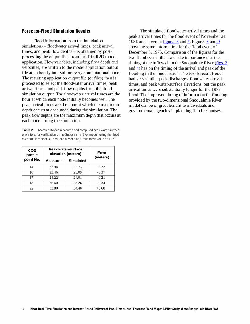
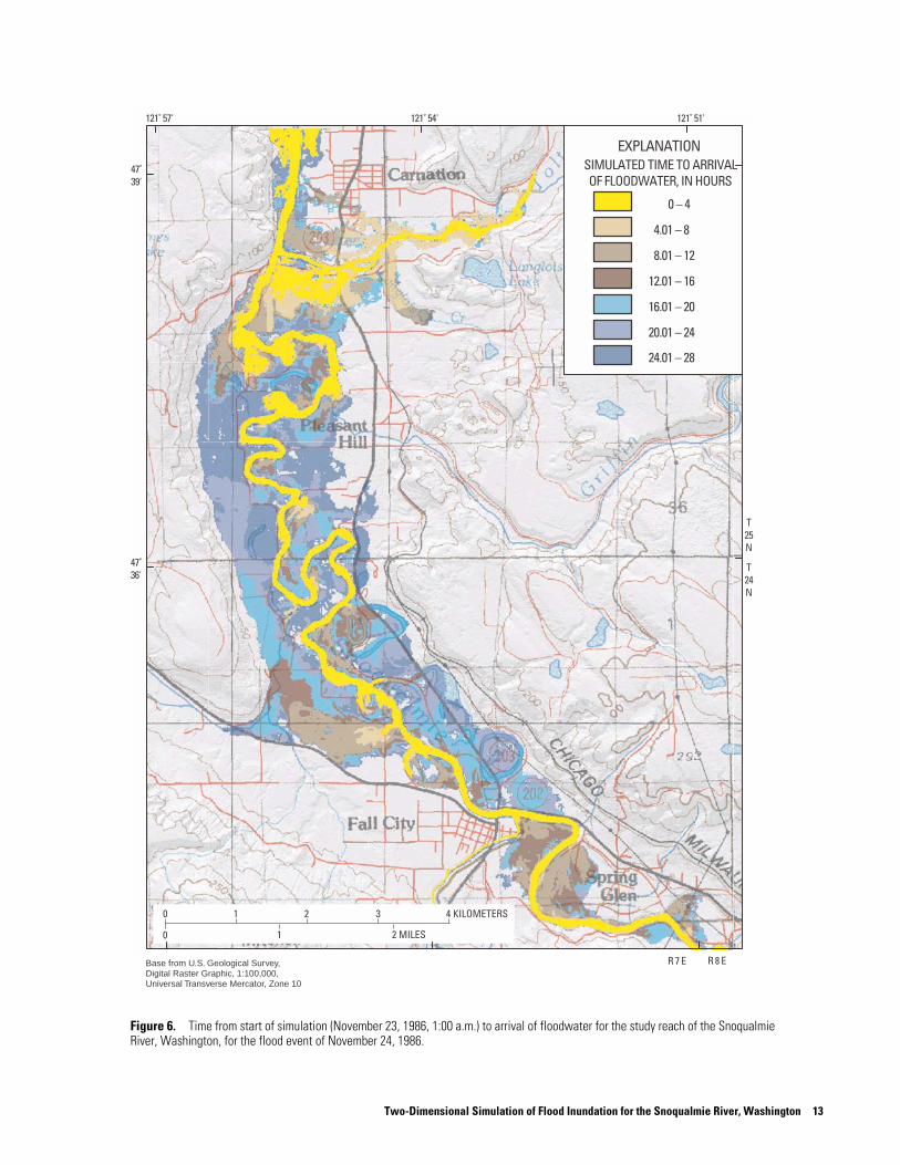
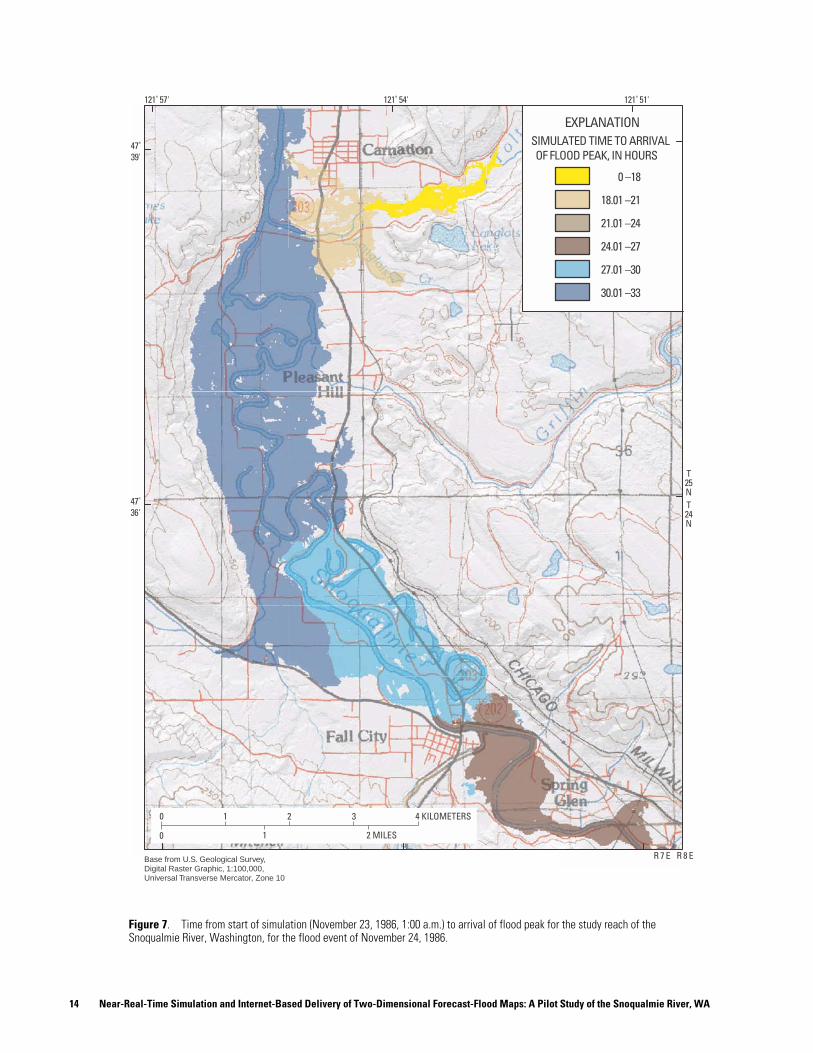
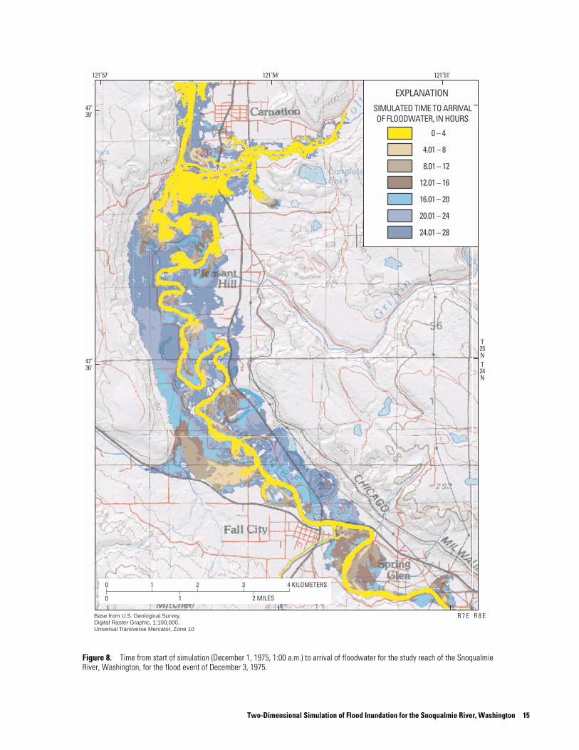
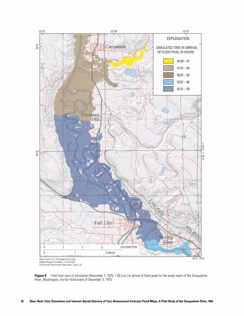
Forecast-Flood Simulation Results

Flood information from the inundation simulations – floodwater arrival times, peak arrival times, and peak flow depths – is obtained by post-processing the output files from the TrimR2D model application. Flow variables, including flow depth and velocities, are written to the model application output file at an hourly interval for every computational node. The resulting application output file (or files) then is processed to select the floodwater arrival times, peak arrival times, and peak flow depths from the flood simulation output. The floodwater arrival times are the hour at which each node initially becomes wet. The peak arrival times are the hour at which the maximum depth occurs at each node during the simulation. The peak flow depths are the maximum depth that occurs at each node during the simulation.

The simulated floodwater arrival times and the peak arrival times for the flood event of November 24, 1986 are shown in figures 6 and 7. Figures 8 and 9 show the same information for the flood event of December 3, 1975. Comparison of the figures for the two flood events illustrates the importance that the timing of the inflows into the Snoqualmie River (figs. 2 and 4) has on the timing of the arrival and peak of the flooding in the model reach. The two forecast floods had very similar peak discharges, floodwater arrival times, and peak water-surface elevations, but the peak arrival times were substantially longer for the 1975 flood. The improved timing of information for flooding provided by the two-dimensional Snoqualmie River model can be of great benefit to individuals and governmental agencies in planning flood responses.

Table 2. Match between measured and computed peak water-surface elevations for verification of the Snoqualmie River model, using the flood event of December 3, 1975, and a Manning’s roughness value of 0.12

COE profile

point No.

Peak water-surface elevation (meters) Error

(meters)Measured Simulated

14 22.94 22.73 -0.22

16 23.46 23.09 -0.37

17 24.22 24.01 -0.21

18 25.60 25.26 -0.34

22 33.80 34.48 +0.68


EXPLANATIONSIMULATED TIME TO ARRIVAL OF FLOODWATER, IN HOURS

0 – 4

4.01 – 8

8.01 – 12

12.01 – 16

16.01 – 20

20.01 – 24

24.01 – 28

0

0

1 2 3 4 KILOMETERS

1 2 MILES

121 ̊57' 121 ̊54' 121 ̊51'

47˚39'

47˚36'

T25N

T24N


Figure 6. Time from start of simulation (November 23, 1986, 1:00 a.m.) to arrival of floodwater for the study reach of the Snoqualmie River, Washington, for the flood event of November 24, 1986.


14 Nea

EXPLANATIONSIMULATED TIME TO ARRIVAL OF FLOOD PEAK, IN HOURS

0 –18

18.01 –21

21.01 –24

24.01 –27

27.01 –30

30.01 –33

0

0

1 2 3 4 KILOMETERS

1 2 MILES

T25NT24N

R 7 E R 8 E

121 ̊57' 121 ̊54' 121 ̊51'

47˚39'

47˚36'

Base from U.S. Geological Survey,Digital Raster Graphic, 1:100,000, Universal Transverse Mercator, Zone 10

r

Figure 7. Time from start of simulation (November 23, 1986, 1:00 a.m.) to arrival of flood peak for the study reach of the Snoqualmie River, Washington, for the flood event of November 24, 1986.

-Real-Time Simulation and Internet-Based Delivery of Two-Dimensional Forecast-Flood Maps: A Pilot Study of the Snoqualmie River, WA

EXPLANATION

SIMULATED TIME TO ARRIVAL OF FLOODWATER, IN HOURS

0 – 4

4.01 – 8

8.01 – 12

12.01 – 16

16.01 – 20

20.01 – 24

24.01 – 28

0

0

1 2 3 4 KILOMETERS

1 2 MILES

121˚57' 121˚54' 121˚51'

47˚39'

47˚36'

T25NT24N


Figure 8. Time from start of simulation (December 1, 1975, 1:00 a.m.) to arrival of floodwater for the study reach of the Snoqualmie River, Washington, for the flood event of December 3, 1975.


16 N

EXPLANATION

SIMULATED TIME OF ARRIVAL OF FLOOD PEAK, IN HOURS

44.00 – 47

47.01 – 50

50.01 – 53

53.01 – 56

65.01 – 59

0

0

1 2 3 4 KILOMETERS

1 2 MILES

T25NT24N

R 7 E R 8 E

121˚57' 121˚54' 121˚51'

47˚39'

47˚36'

Base from U.S. Geological Survey,Digital Raster Graphic, 1:100,000, Universal Transverse Mercator, Zone 10

Figure 9. Time from start of simulation (December 1, 1975, 1:00 a.m.) to arrival of flood peak for the study reach of the Snoqualmie River, Washington, for the flood event of December 3, 1975.

ear-Real-Time Simulation and Internet-Based Delivery of Two-Dimensional Forecast-Flood Maps: A Pilot Study of the Snoqualmie River, WA

AUTOMATED PROCESSING AND DISPLAY OF FORECAST-FLOOD INFORMATION

The simulation of forecast floods, the creation of inundation maps, and their delivery on Internet were automated by a file-processing program. The automated file-processing program performs two file-conversion processes.

• Retrieves the daily flood-forecast file from the National Weather Service Northwest River Forecast Center and reformats it to be used as input for TrimR2D. Before TrimR2D is run, the program retrieves a flood-forecast file containing a 3-to-5-day forecast of flood stages and flows for sites in the study area from the RFC in Portland, Oreg. The program then selectively reads data from the river forecast file and writes it to a new file in the format required by the model.

• Converts TrimR2D output data formatted as ASCII files into shape files, a geographically referenced graphics exchanged file format. After TrimR2D is applied to generate simulated flood forecast conditions, the program converts TrimR2D output files, which are in an ASCII format, to shape files.

The shape files are then imported into a MapGuide© Internet map server application for display on the Internet.

File-Processing Program Interface

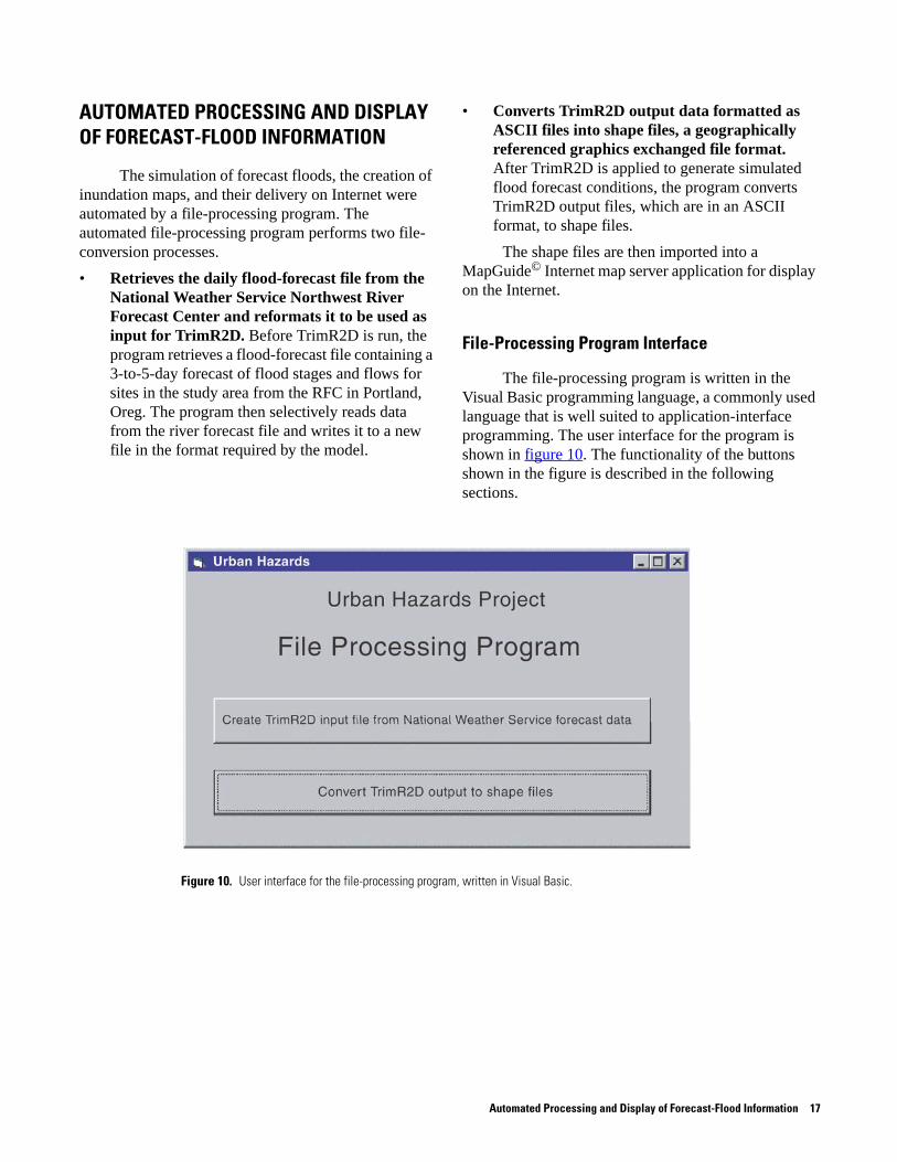
The file-processing program is written in the Visual Basic programming language, a commonly used language that is well suited to application-interface programming. The user interface for the program is shown in figure 10. The functionality of the buttons shown in the figure is described in the following sections.

Figure 10. User interface for the file-processing program, written in Visual Basic.

Automated Processing and Display of Forecast-Flood Information 17

Creating TrimR2D Input File From National Weather Service River Forecast Center Forecast Data

The process of creating flood forecast maps starts by executing the batch file getfile.bat (table 3 and appendix A.1), which contains an FTP command that opens a connection to an NWS computer in Portland, Oreg., and then executes the commands in the log.ftp file (table 3 and appendix A.2). A copy of the river forecast file from the RFC computer is retrieved and placed in a directory on a USGS computer. The

retrieved river forecast file is formatted in a Standard Hydrometeorological Exchange Format (SHEF), which the NWS developed for interagency data sharing (documentation on the SHEF format can be obtained at the URL http://weather.gov/oh/hrl/shef/ version_1.2/index.htm). The automated process then executes Visual Basic code (appendix A.3) that reads through the river forecast file and selects forecast values for stage at the Snoqualmie River near Carnation site, flow at the Snoqualmie River near Snoqualmie site, and flow at the Tolt River near the Carnation site.

18 Ne

.Table 3. Type, purpose, source, and use of files used in the file-processing program

File Type and purpose of file Created by Used by

getfile.bat Batch file containing file transfer protocol (FTP) commands for connecting the USGS server to the NWS server and for calling the log.ftp file

Author File processing program

log.ftp File containing ftp commands for retrieving the river forecast file from the NWS server

Author getfile.bat

storm.txt File containing a 3- to 5-day forecast of river stage or flow data for the Snoqualmie River near Snoqualmie, Wash. and near Carnation, Wash., and the Tolt River near Carnation, Wash.

log.ftp File processing program

modelInput.txt ASCII input file for TrimR2D model containing river stage and flow data for Snoqualmie River near Snoqualmie, Wash., Tolt River near Carnation, Wash., and Snoqualmie River near Carnation, Wash.

File processing program

TrimR2D

FloodDepthgis.txt ASCII file containing TrimR2D simulation of maximum flood depth at all locations in the modeled reach

File processing program using TrimR2D output

shape.aml

ArrivalTimegis.txt ASCII file containing TrimR2D simulation of times when maximum flood depth will occur at locations in the modeled reach


shape.aml

WetTimegis.txt ASCII file containing TrimR2D simulation of times when floodwater first reaches locations in the study area


shape.aml

Floodshape Shape file of maximum flood depth at locations in the study area

shape.aml Internet map server

Arrivalshape Shape file of time when maximum flood depth will occur at locations in the study area


Wetshape Shape file of time when floodwater first reaches locations in the study area


ar-Real-Time Simulation and Internet-Based Delivery of Two-Dimensional Forecast-Flood Maps: A Pilot Study of the Snoqualmie River, WA

http://weather.gov/oh/hrl/shef/version_1.2/index.htm


Flows at the Raging River site are estimated using eq. 1. The flow values for the Snoqualmie River near Carnation and the Raging River near Falls City, the flow estimates for the Tolt River near Carnation and the stage for the Snoqualmie River near Carnation are written to a fixed-format ASCII file for input into TrimR2D (modelInput.txt, table 3 and (appendixA.4). Simulations of flow and stage for the model domain then are made by using Trim2D.

Converting TrimR2D Output to Shape Files

Three output files are created by TrimR2D: a file containing maximum flood depth for all locations in the study area (FloodDepthgis.txt, table 3); a file containing the times the maximum flood depth is predicted to occur at all locations in the study area (ArrivalTimegis.txt, table 3); and a file containing the times that all locations in the study area are first reached by floodwater (WetTimegis.txt, table 3). The three files output from TrimR2D are formatted ASCII files and must be converted to a spatial data format (shape files) that can be displayed on the Internet.

Shape files are created by executing Visual Basic application program interface (API) code (appendix A.5) that starts ArcInfo software installed on the user's computer and then executing the shape.aml file. The shape.aml file (table 3 and appendix A.6) is written in the Arc Macro Language and contains all the commands used to convert the TrimR2D output files from ASCII format to shape files. The ASCIIGRID command in shape.aml converts the ASCII files from TrimR2D into GRIDs, a spatial data format used by ArcInfo for raster data. Commands then are executed to aggregate the values for the maximum flood depth into three categories: 0-to-2 foot depth, 2-to-5-foot depth, and greater than a 5-foot depth. Finally, the GRIDSHAPE command executes and converts the GRIDs into three shape files (table 3). The shape files then are copied to a directory where they can be imported to the Internet map server and displayed on the Internet.

The file-processing program can be run on a PC or server with the Microsoft NT 4.0 or Windows 2000 operating system and the geographic information system ArcInfo (version 7.0 or greater) installed. Recommended RAM for running ArcInfo is 500 megabytes.

INTERNET MAP SERVER DEVELOPMENT

Internet map servers (IMSs) are an emerging software technology developed specifically to allow greater flexibility for the authors and viewers of digital maps. The authors of an IMS application have the ability to control the map components and their appearance according to the scale selected by the viewer; the viewers have the ability to select map components the author has made available and to select features to view based on geographical or data-based queries. For example, a map component of a residential road network would be too detailed for a small-scale map (perhaps a several-county area), so the author would not offer that component at that scale, but may make it active only at larger scales where the network does not overly clutter the map. The viewer may be given the choice of a topographic map or an aerial photograph to use as the background for, in this case, a map of flood inundation.

Numerous IMSs are currently on the market, and they generally have the features described above. Each has unique features, various strengths and weaknesses, and they are evolving quickly. The approach for map authors, however, is quite similar. The source of map components may be a GIS or a Computer Aided Drafting (CAD) package or other geographically referenced relational database program. These components are converted to the proper format for import into the IMS, most of which have robust import routines. Once imported into the IMS, the author of the map application has the ability to select the scale at which each component is viewable. The author also has the ability to change the appearance of the component at specific scales – a highway map, for example, may be made to appear as a single red line at the smallest scale, whereas at larger scales it may appear as a composite red and black line to distinguish it from local roads. Pixel-based, or raster, images may be compressed for viewing at small (regional) scales for quick Internet transfer, and progressively be delivered at greater and greater resolution as smaller geographic areas are selected for viewing.

Automated Processing and Display of Forecast-Flood Information 19

SUMMARY

The U.S. Geological Survey combined new data sources, new computational techniques, and new map creation and delivery software systems to pilot near-real-time mapping of forecast or imminent flooding as part of its Urban Geologic and Hydrologic Natural Hazards Initiative. The new mapping method was demonstrated in a pilot study for a reach of the Snoqualmie River in Washington State. New data sources provide high-accuracy, areally dense elevation data; new computational techniques provide a robust and stable two-dimensional hydraulic model capable of simulating a wide range of flooding situations on longer river reaches than were previously possible; and new software systems allow the post-processing of simulations into flood inundation and depth maps that can be delivered over the Internet in a flexible and user-friendly way.

This report documents the calibration and verification of TrimR2D for a 28-kilometer reach of the Snoqualmie River and the simulation of flood inundation for the reach; and describes the automated processing and display of the forecast floodforecast-flood inundation simulation. The discussion of automation includes processing of the model output into flood-extent and -depth maps with a Geographic Information System; processing of the maps for the Internet map server; Internet map server authoring; and automation of the entire process using Visual Basic. Sufficient detail is provided to allow subsequent investigators to duplicate and(or) improve on the methodology.

The only flood maps available for most areas are maps prepared for the Federal flood insurance program. Because these maps are the best, often the only, source of information about flooding potential, they are also used for essentially all flood planning and mitigation purposes. Officials planning for or responding to flooding would benefit from flood information relating specifically to an imminent flooding event. The National Weather Service forecasts flood flows and elevations at forecast points for actual approaching storms, but currently no one estimates inundation associated with the forecast flood.

Information about flood extent and depth for a storm-specific flood would aid emergency response officials in identifying the areas where their resources are needed the most immediately or critically. Elevation data of adequate accuracy to use in hydraulic flow models have been prohibitively expensive, and therefore typically have been gathered only for cross sections (for use in one-dimensional models). Now, LIght Detection and Ranging (LIDAR) technology makes very-high-accuracy elevation data (accurate to 15 centimeters or about half a foot) affordable, especially considering the variety of applications it is suited for. The relatively new TrimR2D hydraulic model, with a computationally very stable solution algorithm, was used for the study. It allows simulation of long reaches, can simulate rapidly changing flows, and is robust enough to handle an input hydrograph without tedious trial-and-error preparation of usable initial conditions. These features make the model uniquely suited to simulating forecast-flood hydrographs in near real time.

Applying the model to the Snoqualmie River involved developing a two-dimensional model grid of ground-surface elevations, specifying upstream and downstream hydraulic boundary conditions, selecting an appropriate computational time step for simulations, calibrating the model to data from a 1986 flood, and verifying the calibration with data from a 1975 flood, both of which had a 0.1 probability of occurrence (10-year frequency).

Inflow discharges and outflow water-surface elevations were available at a 1-hour time interval for both floods. Measured high-water marks were available for both floods at five profile points from the U.S. Army Corps of Engineers (COE), but data were not available for comparing simulated and actual inundated areas.

The average error for the 1986 calibration flood was -0.14 meter and the average absolute error was 0.41 meter for the COE observation points. The average error for the 1975 verification flood was -0.09 meter and the average absolute error was 0.36 meter for the COE observation points. For both calibration and verification, water-surface elevations were overestimated at the upstream observation points and underestimated at downstream points.


The Snoqualmie River model forecast-flood inundation simulation uses NWS flood forecasts at the Snoqualmie River near Snoqualmie, the Tolt River near Carnation, and the Snoqualmie River near Carnation. Flows and water-surface elevations are forecast at 6-hour intervals by the NWS River Forecast Center (RFC) in Portland, Oregon. Forecast data are downloaded from the RFC computers and are automatically processed automatically for input into the Snoqualmie River model. The Snoqualmie River model then is executed using the processed NWS forecast data. Flood information from the inundation simulations – floodwater arrival times, peak arrival times, and peak flow depths – is obtained by post-processing the output files from the TrimR2D model application. Geographic Information System software is used to post-process model data to produce flood extent and depth maps that are further processed into a format compatible with the Internet map server (IMS) software. IMS software is a relatively new technology that allows the map audience greater control over what they see and at what scale they see it. Finally, all of the required pieces – forecast acquisition, flow modeling, map generation, and map presentation – are automated using Visual Basic, one of the most ubiquitous current programming languages.

The complete process results in automated retrieval and processing of NWS flood forecasts for input into the hydraulic model. Results for the 28-kilometer reach of the Snoqualmie River subsequently are automatically processed into maps of depth of flood, time of arrival, and time of peak that are ready for input to the Internet map server, which presents the information over the Internet in a user-friendly format.

REFERENCES

Albertson, M.L., Barton, J.R., and Simons, D.B., 1960, Fluid mechanics for engineers: Englewood Cliffs, N.J., Prentice-Hall, 561 p.

Casulli, V., 1990, Semi-implicit finite difference methods for the two-dimensional shallow water equations: Journal of Computational Physics, v. 86, p.56-74.

Cheng, R.T., Casulli, V., and Gartner, J.W., 1993, Tidal, residual, intertidal mudflat (TRIM) model and its applications to San Francisco Bay, California: Estuarine, Coastal and Shelf Science, v.36, p. 235-280.

Jones, J.L., Haluska, T.L., and Kresch, D.L., 2001, Updating flood maps efficiently using existing hydraulic model, very-high-accuracy elevation data, and a geographic information system – a pilot study on the Nisqually River, Washington: U.S. Geological Survey Water-Resources Investigations Report 01-4051, 25 p.

National Weather Service Office of Hydrology, 1996, Weather Service hydrology handbook No. 1, Standard hydrometeorological exchange format version 1.2, accessed September 11, 2002, at URL: http://weather.gov/oh/hrl/shef/version_1.2/index.htm.

Ostenaa, D.A., Levish, D.R., Klinger, R.E., and O'Connell, D.R.H., 1999, Phase 2 paleohydrologic and geomorphic studies for the assessment of flood risk for the Idaho National Engineering and Environmental Laboratory, Idaho: Bureau of Reclamation Report 99-7, 117 p.

Rouse, H., ed., 1950, Engineering Hydraulics – Proceedings of the Fourth Hydraulics Conference, Iowa Institute of Hydraulic Research, June 12-15, 1949: New York, John Wiley & sons, 1039 p.

Staniforth A., and Cote, J., 1991, Semi-lagrangian integration schemes for atmospheric models – a review: American Meteorological Society Monthly Weather Review, v.119, p. 2206-2223.

U.S. Army Corps of Engineers Waterways Experiment Station Hydraulics Laboratory, 1996, RMA2 Version 4.3, 02.28.1996, 227 p.

References 21


APPENDIX A. FILE PROCESSING PROGRAMS AND MODEL INPUT EXAMPLE FILE

Appendix A1. Contents of getfile.bat file

ftp -s:log.ftp <NWS server name omitted for security>

copy *snohomish storm.txt

move *snohomish oldstorms\.

Appendix A2. Contents of log.ftp file

<user name omitted for security><user password omitted for security>cd pub/usgsmget *.snohomishybye

Appendix A. File Processing Programs and Model Input Example File 22

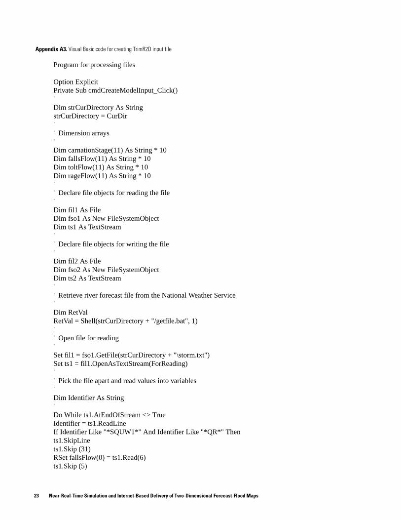
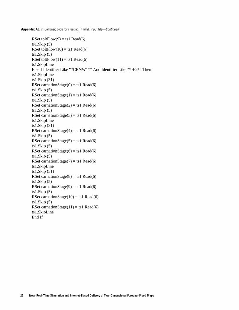
Appendix A3. Visual Basic code for creating TrimR2D input file

Program for processing files

Option ExplicitPrivate Sub cmdCreateModelInput_Click()'Dim strCurDirectory As StringstrCurDirectory = CurDir'' Dimension arrays'Dim carnationStage(11) As String * 10Dim fallsFlow(11) As String * 10Dim toltFlow(11) As String * 10Dim rageFlow(11) As String * 10'' Declare file objects for reading the file'Dim fil1 As FileDim fso1 As New FileSystemObjectDim ts1 As TextStream'' Declare file objects for writing the file'Dim fil2 As FileDim fso2 As New FileSystemObjectDim ts2 As TextStream'' Retrieve river forecast file from the National Weather Service'Dim RetValRetVal = Shell(strCurDirectory + "/getfile.bat", 1)'' Open file for reading'Set fil1 = fso1.GetFile(strCurDirectory + "\storm.txt")Set ts1 = fil1.OpenAsTextStream(ForReading)'' Pick the file apart and read values into variables'Dim Identifier As String'Do While ts1.AtEndOfStream <> TrueIdentifier = ts1.ReadLineIf Identifier Like "*SQUW1*" And Identifier Like "*QR*" Thents1.SkipLinets1.Skip (31)RSet fallsFlow(0) = ts1.Read(6)ts1.Skip (5)

23 Near-Real-Time Simulation and Internet-Based Delivery of Two-Dimensional Forecast-Flood Maps

Appendix A3. Visual Basic code for creating TrimR2D input file—Continued

RSet fallsFlow(1) = ts1.Read(6)ts1.Skip (5)RSet fallsFlow(2) = ts1.Read(6)ts1.Skip (5)RSet fallsFlow(3) = ts1.Read(6)ts1.SkipLinets1.Skip (31)RSet fallsFlow(4) = ts1.Read(6)ts1.Skip (5)RSet fallsFlow(5) = ts1.Read(6)ts1.Skip (5)RSet fallsFlow(6) = ts1.Read(6)ts1.Skip (5)RSet fallsFlow(7) = ts1.Read(6)ts1.SkipLinets1.Skip (31)RSet fallsFlow(8) = ts1.Read(6)ts1.Skip (5)RSet fallsFlow(9) = ts1.Read(6)ts1.Skip (5)RSet fallsFlow(10) = ts1.Read(6)ts1.Skip (5)RSet fallsFlow(11) = ts1.Read(6)ts1.SkipLineElseIf Identifier Like "*STOW1*" And Identifier Like "*QR*" Thents1.SkipLinets1.Skip (31)RSet toltFlow(0) = ts1.Read(6)ts1.Skip (5)RSet toltFlow(1) = ts1.Read(6)ts1.Skip (5)RSet toltFlow(2) = ts1.Read(6)ts1.Skip (5)RSet toltFlow(3) = ts1.Read(6)ts1.SkipLinets1.Skip (31)RSet toltFlow(4) = ts1.Read(6)ts1.Skip (5)RSet toltFlow(5) = ts1.Read(6)ts1.Skip (5)RSet toltFlow(6) = ts1.Read(6)ts1.Skip (5)RSet toltFlow(7) = ts1.Read(6)ts1.SkipLinets1.Skip (31)RSet toltFlow(8) = ts1.Read(6)ts1.Skip (5)



RSet toltFlow(9) = ts1.Read(6)ts1.Skip (5)RSet toltFlow(10) = ts1.Read(6)ts1.Skip (5)RSet toltFlow(11) = ts1.Read(6)ts1.SkipLineElseIf Identifier Like "*CRNW1*" And Identifier Like "*HG*" Thents1.SkipLinets1.Skip (31)RSet carnationStage(0) = ts1.Read(6)ts1.Skip (5)RSet carnationStage(1) = ts1.Read(6)ts1.Skip (5)RSet carnationStage(2) = ts1.Read(6)ts1.Skip (5)RSet carnationStage(3) = ts1.Read(6)ts1.SkipLinets1.Skip (31)RSet carnationStage(4) = ts1.Read(6)ts1.Skip (5)RSet carnationStage(5) = ts1.Read(6)ts1.Skip (5)RSet carnationStage(6) = ts1.Read(6)ts1.Skip (5)RSet carnationStage(7) = ts1.Read(6)ts1.SkipLinets1.Skip (31)RSet carnationStage(8) = ts1.Read(6)ts1.Skip (5)RSet carnationStage(9) = ts1.Read(6)ts1.Skip (5)RSet carnationStage(10) = ts1.Read(6)ts1.Skip (5)RSet carnationStage(11) = ts1.Read(6)ts1.SkipLineEnd If



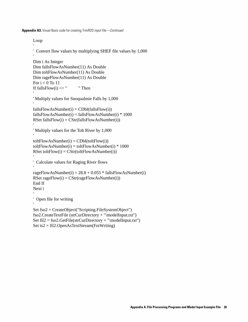
Loop'' Convert flow values by multiplying SHEF file values by 1,000'Dim i As IntegerDim fallsFlowAsNumber(11) As DoubleDim toltFlowAsNumber(11) As DoubleDim rageFlowAsNumber(11) As DoubleFor i = 0 To 11If fallsFlow(i) <> " " Then'' Multiply values for Snoqualmie Falls by 1,000'fallsFlowAsNumber(i) = CDbl(fallsFlow(i))fallsFlowAsNumber(i) = fallsFlowAsNumber(i) * 1000RSet fallsFlow(i) = CStr(fallsFlowAsNumber(i))'' Multiply values for the Tolt River by 1,000'toltFlowAsNumber(i) = CDbl(toltFlow(i))toltFlowAsNumber(i) = toltFlowAsNumber(i) * 1000RSet toltFlow(i) = CStr(toltFlowAsNumber(i))'' Calculate values for Raging River flows'rageFlowAsNumber(i) = 28.8 + 0.055 * fallsFlowAsNumber(i)RSet rageFlow(i) = CStr(rageFlowAsNumber(i))End IfNext i'' Open file for writing'Set fso2 = CreateObject("Scripting.FileSystemObject")fso2.CreateTextFile (strCurDirectory + "\modelInput.txt")Set fil2 = fso2.GetFile(strCurDirectory + "\modelInput.txt")Set ts2 = fil2.OpenAsTextStream(ForWriting)


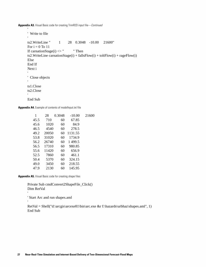
Appendix A3. Visual Basic code for creating TrimR2D input file—Continued'' Write to file'ts2.WriteLine " 1 28 0.3048 -10.00 21600"For i = 0 To 11If carnationStage(i) <> " " Thents2.WriteLine carnationStage(i) + fallsFlow(i) + toltFlow(i) + rageFlow(i)ElseEnd IfNext i'' Close objects'ts1.Closets2.Close'End Sub

Appendix A4. Example of contents of modelInput.txt file

1 28 0.3048 -10.00 21600 45.5 710 60 67.85 45.6 1020 60 84.9 46.5 4540 60 278.5 49.2 20050 60 1131.55 53.8 31020 60 1734.9 56.2 26740 60 1 499.5 56.5 17310 60 980.85 55.6 11420 60 656.9 52.5 7860 60 461.1 50.4 5370 60 324.15 49.0 3450 60 218.55 47.9 2130 60 145.95

Appendix A5. Visual Basic code for creating shape files

Private Sub cmdConvert2ShapeFile_Click()Dim RetVal'' Start Arc and run shapes.aml'RetVal = Shell("d:\arcgis\arcexe81\bin\arc.exe &r f:\hazards\urbhaz\shapes.aml", 1)End Sub


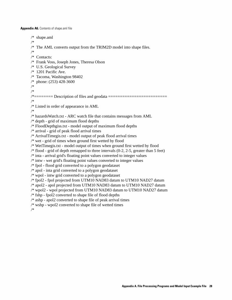
Appendix A6. Contents of shape.aml file

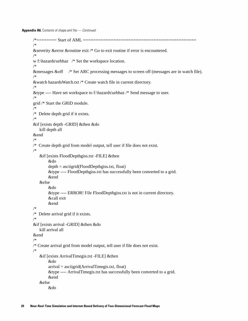
/* shape.aml/* /* The AML converts output from the TRIM2D model into shape files./*/* Contacts:/* Frank Voss, Joseph Jones, Theresa Olson/* U.S. Geological Survey/* 1201 Pacific Ave./* Tacoma, Washington 98402/* phone: (253) 428-3600/*/*/*======== Description of files and geodata =========================/*/* Listed in order of appearance in AML/*/* hazardsWatch.txt - ARC watch file that contains messages from AML/* depth - grid of maximum flood depths/* FloodDepthgiss.txt - model output of maximum flood depths/* arrival - grid of peak flood arrival times/* ArrivalTimegis.txt - model output of peak flood arrival times/* wet - grid of times when ground first wetted by flood/* WetTimegis.txt - model output of times when ground first wetted by flood/* flood - grid of depth remapped to three intervals (0-2, 2-5, greater than 5 feet)/* inta - arrival grid's floating point values converted to integer values/* intw - wet grid's floating point values converted to integer values/* fpol - flood grid converted to a polygon geodataset/* apol - inta grid converted to a polygon geodataset/* wpol - intw grid converted to a polygon geodataset/* fpol2 - fpol projected from UTM10 NAD83 datum to UTM10 NAD27 datum/* apol2 - apol projected from UTM10 NAD83 datum to UTM10 NAD27 datum/* wpol2 - wpol projected from UTM10 NAD83 datum to UTM10 NAD27 datum/* fshp - fpol2 converted to shape file of flood depths/* ashp - apol2 converted to shape file of peak arrival times/* wshp - wpol2 converted to shape file of wetted times/*


Appendix A6. Contents of shape.aml file — Continued

/*======== Start of AML =============================================/*&severity &error &routine exit /* Go to exit routine if error is encountered./*w f:\hazards\urbhaz /* Set the workspace location./*&messages &off /* Set ARC processing messages to screen off (messages are in watch file)./*&watch hazardsWatch.txt /* Create watch file in current directory./*&type ---- Have set workspace to f:\hazards\urbhaz /* Send message to user./* grid /* Start the GRID module./*/* Delete depth grid if it exists./*&if [exists depth -GRID] &then &do

kill depth all&end/*/* Create depth grid from model output, tell user if file does not exist./*

&if [exists FloodDepthgiss.txt -FILE] &then&dodepth = asciigrid(FloodDepthgiss.txt, float)&type ---- FloodDepthgiss.txt has successfully been converted to a grid.&end

&else&do&type ---- ERROR! File FloodDepthgiss.txt is not in current directory.&call exit&end

/*/* Delete arrival grid if it exists./*&if [exists arrival -GRID] &then &do

kill arrival all&end/*/* Create arrival grid from model output, tell user if file does not exist./*

&if [exists ArrivalTimegis.txt -FILE] &then&doarrival = asciigrid(ArrivalTimegis.txt, float)&type ---- ArrivalTimegis.txt has successfully been converted to a grid. &end

&else&do



&type ---- ERROR! File ArrivalTimegis.txt is not in current directory.&call exit&end

/*/* Delete wet grid if it exists./*&if [exists wet -GRID] &then &do

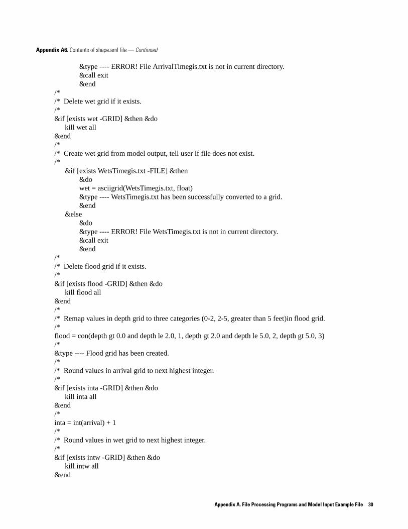
kill wet all&end/*/* Create wet grid from model output, tell user if file does not exist./*

&if [exists WetsTimegis.txt -FILE] &then&dowet = asciigrid(WetsTimegis.txt, float)&type ---- WetsTimegis.txt has been successfully converted to a grid.&end

&else&do&type ---- ERROR! File WetsTimegis.txt is not in current directory.&call exit&end

/*/* Delete flood grid if it exists./*&if [exists flood -GRID] &then &do

kill flood all&end/*/* Remap values in depth grid to three categories (0-2, 2-5, greater than 5 feet)in flood grid./*flood = con(depth gt 0.0 and depth le 2.0, 1, depth gt 2.0 and depth le 5.0, 2, depth gt 5.0, 3)/*&type ---- Flood grid has been created./*/* Round values in arrival grid to next highest integer./*&if [exists inta -GRID] &then &do

kill inta all&end/*inta = int(arrival) + 1/*/* Round values in wet grid to next highest integer./*&if [exists intw -GRID] &then &do

kill intw all&end



intw = int(wet) + 1/*/* Convert grids to polygons./*&if [exists fpol -POLY] &then &do

kill fpol all&endfpol = gridpoly(flood)&type ---- The flood polygon has been created./*&if [exists apol -POLY] &then &do

kill apol all&endapol = gridpoly(inta)&type ---- The arrival polygon has been created./*&if [exists wpol -POLY] &then &do

kill wpol all&endwpol = gridpoly(intw)&type ---- The wet polygon has been created./*quit /* Quit the GRID module./*/* Project from NAD83 to NAD27/*&if [exists fpol2 -POLY] &then &do

kill fpol2 all&endproject cover fpol fpol2 utmto27.txtclean fpol2&type ---- The flood polygon has been projected./*&if [exists apol2 -POLY] &then &do

kill apol2 all&endproject cover apol apol2 utmto27.txtclean apol2&type ---- The arrival polygon has been projected./*&if [exists wpol2 -POLY] &then &do

kill wpol2 all&endproject cover wpol wpol2 utmto27.txtclean wpol2&type ---- The wet polygon has been projected./*


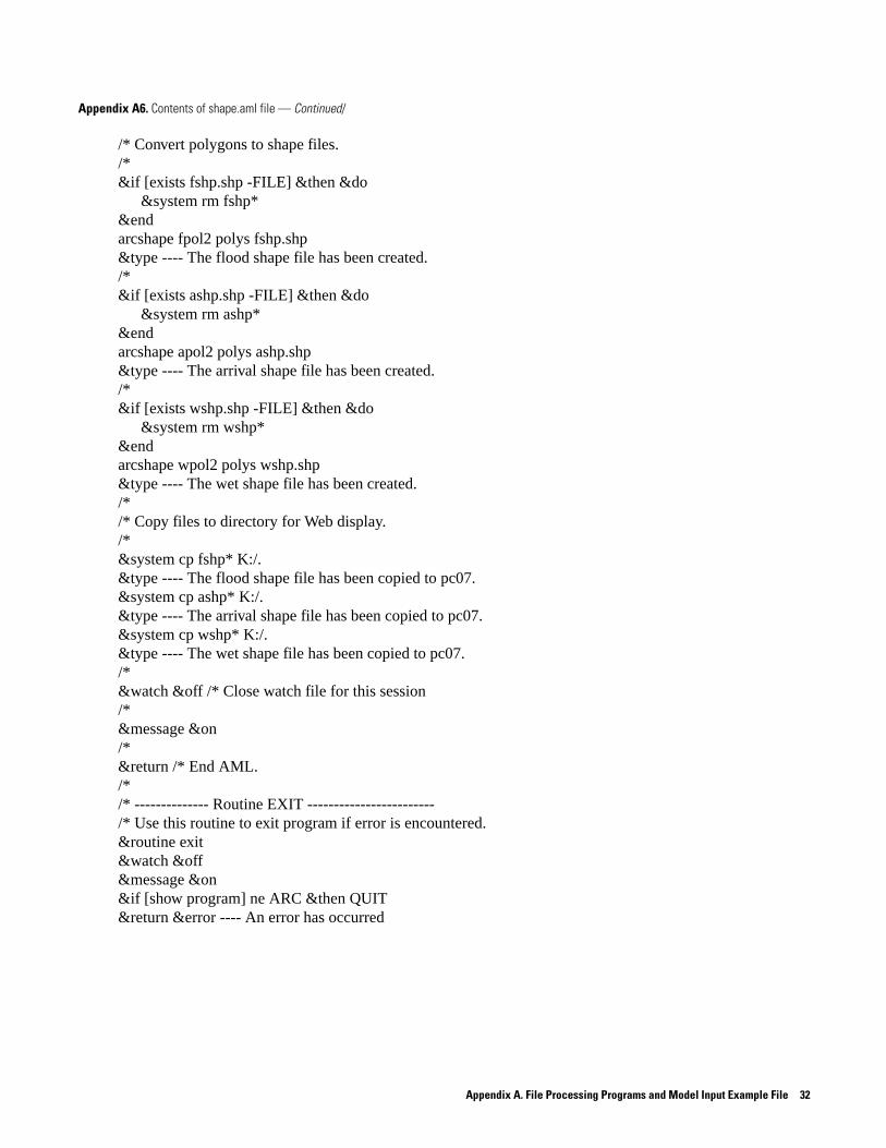
Appendix A6. Contents of shape.aml file — Continued/

/* Convert polygons to shape files./*&if [exists fshp.shp -FILE] &then &do

&system rm fshp*&endarcshape fpol2 polys fshp.shp&type ---- The flood shape file has been created./*&if [exists ashp.shp -FILE] &then &do

&system rm ashp*&endarcshape apol2 polys ashp.shp&type ---- The arrival shape file has been created./*&if [exists wshp.shp -FILE] &then &do

&system rm wshp*&endarcshape wpol2 polys wshp.shp&type ---- The wet shape file has been created./*/* Copy files to directory for Web display./*&system cp fshp* K:/.&type ---- The flood shape file has been copied to pc07.&system cp ashp* K:/.&type ---- The arrival shape file has been copied to pc07.&system cp wshp* K:/.&type ---- The wet shape file has been copied to pc07./*&watch &off /* Close watch file for this session/*&message &on/*&return /* End AML./*/* -------------- Routine EXIT ------------------------/* Use this routine to exit program if error is encountered.&routine exit&watch &off&message &on&if [show program] ne ARC &then QUIT&return &error ---- An error has occurred


Forecast-Flood Inundation Maps: Pilot Study of the Snoqualm

ie River, Washington

Forecast-Flood Inundation Maps: Pilot Study of the Snoqualm

ie River, Washington

Jones and othersJones and others

WRIR 02-4251

Near-Real-Time Simulation and Internet-Based

Documents