Near-field and far-field simulation of accelerograms of Sikkim earthquake of September 18, 2011 using modified semi-empirical approach

ORI GIN AL PA PER

Near-field and far-field simulation of accelerogramsof Sikkim earthquake of September 18, 2011 usingmodified semi-empirical approach

A. Joshi • Pushpa Kumari • Sandeep Singh • M. L. Sharma

Received: 6 March 2012 / Accepted: 5 July 2012 / Published online: 29 August 2012� Springer Science+Business Media B.V. 2012

Abstract The semi-empirical approach for modeling of strong ground motion given by

Midorikawa (Tectonophysics 218:287–295, 1993) has been modified in the present paper

for component wise simulation of strong ground motion. The modified approach uses

seismic moment in place of attenuation relation for scaling of acceleration envelope.

Various strong motion properties like directivity effect and dependence of peak ground

acceleration with respect to surface projection of source model have been studied in detail

in the present work. Recently, Sikkim earthquake of magnitude 6.9 (Mw) that occurred on

September 18, 2011 has been recorded at various near-field and far-field strong motion

stations. The modified semi-empirical technique has been used to confirm the location and

parameters of rupture responsible for this earthquake. Strong motion record obtained from

the iterative modeling of the rupture plane has been compared with available strong motion

records from near as well as far-field stations in terms of root mean square error between

observed and simulated records. Several possibilities of nucleation point, rupture velocity,

and dip of rupture plane have been considered in the present work and records have been

simulated at near-field stations. Final selection of model parameters is based on root mean

square error of waveform comparison. Final model confirms southward propagating rup-

ture. Simulations at three near-field and twelve far-field stations have been made using final

model. Comparison of simulated and observed record has been made in terms of peak

ground acceleration and response spectra at 5 % damping. Comparison of simulated and

observed record suggests that the method is capable of simulating record which bears

realistic appearance in terms of shape and strong motion parameters. Present work shows

A. Joshi � P. Kumari (&) � S. SinghDepartment of Earth Sciences, Indian Institute of Technology Roorkee, Roorkee, Indiae-mail: [email protected]

A. Joshie-mail: [email protected]

M. L. SharmaDepartment of Earthquake Engineering, Indian Institute of Technology Roorkee, Roorkee, India

123

Nat Hazards (2012) 64:1029–1054DOI 10.1007/s11069-012-0281-7

that this technique gives records which matches in a wide frequency range for Sikkim

earthquake and that too from simple and easily accessible parameters of the rupture plane.

Keywords Strong ground motion � Semi-empirical � Sikkim earthquake � Parameters

1 Introduction

Strong ground motion plays an important role in safe engineering design of big structures.

The site of construction seldom contains any past strong motion records that pose a major

constrain in designing earthquake-resistant design parameters. Simulated strong motion

records at such sites serve useful purpose for deciding safe design criteria. There are

number of simulation technique that can be used for simulation of strong ground motion.

Three main techniques for simulation of strong ground motion are (1) stochastic simulation

technique (Housner and Jennings 1964; Hanks and McGuire 1981; Boore 1983; McGuire

et al. 1984; Boore and Joyner 1991; Sinozuka and Sato 1967; Lai 1982), (2) empirical

Green’s function technique (Hartzell 1978, 1982; Kanamori 1979; Hadley and Helmberger

1980; Mikumo et al. 1981; Irikura and Muramatu 1982; Hadley et al. 1982; Irikura 1983;

Houston and Kanamori 1984; Imagawa et al. 1984; Munguia and Brune 1984; Hutchings

1985; Heaton and Hartzell 1989), and (3) composite source modeling technique (Zeng

et al. 1994; Yu 1994; Yu et al. 1995). Although the stochastic simulation technique gives

encouraging results for many regions, it does not include any representation of finite

earthquake source and wave propagation in the medium. Empirical Green’s function

technique is most reliable technique in terms of strong motion characterization. In this

technique, there is no need to remove propagation effects (Fukuyama and Irikura 1986).

The small earthquake record needed in this method as empirical Green’s function is

required from the site at which simulation of target earthquake is needed (Joyner and Boore

1988). This is the most difficult condition to be met in practice and hence the method is of

limited use. The method of composite source modeling takes into account the random

nature of the complex source slip function together with the use of theoretical Green’s

function (Khattri et al. 1994). One of the major disadvantages in this technique is its

requirement of several parameters for computing synthetic Green’s function which are

difficult to predict.

In the recent years, the method of modified semi-empirical simulation of strong ground

motion has been evolved as an effective tool for prediction of strong motion. This method

has advantage of both the empirical Green’s function technique and stochastic simulation

technique. The method of semi-empirical modeling has been given by Midorikawa (1993)

and later modified by Joshi and Midorikawa (2004). In this technique, synthetic records

from different sub-faults within the rupture plane are used in place of aftershock records as

Green’s function. The advantage of the proposed semi-empirical technique is that it is very

fast to calculate and is based on simple attenuation relations and modeling parameters

which are easy to predict. The semi-empirical method is used for simulation of strong

motion records by Joshi (2004), Joshi and Midorikawa (2004), and Joshi et al. (2010).

However, dependency of semi-empirical method on attenuation relation itself poses a

constraint on its applicability for its use in different seismic environment. In order to

remove dependency of this method on attenuation relation, the method was modified by

Joshi et al. (2012) to incorporate seismic moment and effect of radiation pattern in it. One

of the major limitations in the simulations using semi-empirical approach is its inability to

resolve records into horizontal component. The method has been further modified in this

1030 Nat Hazards (2012) 64:1029–1054

123

work to resolve the obtained record into horizontal components. The simulated records

obtained in the modified method have been tested with the data of the recent Sikkim

earthquake (Mw = 6.9) of September 18, 2011. The method is used to finalize various

rupture parameters of this earthquake by iterative forward modeling.

1.1 Geological framework

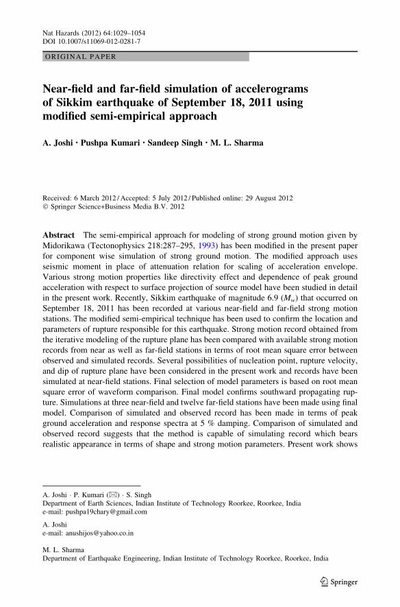
The Sikkim Himalaya lies in eastern region with well-mapped geological and tectonic units

(Fig. 1) having classic inverted Himalayan metamorphism. Geologically, the Sikkim

Himalaya exhibits a vast terrain of proterozoic continental crust on the Indian plate, which

is remobilized into vast slab-like Higher Himalayan crystallines (HHC) due to Himalayan

collision tectonics. This unit is bounded by the Main Central Thrust (MCT) at the base and

the South Tibetan Detachment Zone (STDZ) at the top (Fig. 1). The Lesser Himalayan

Sedimentary Zone (Buxa, Permian Ranjit Pebble Slate/Damuda Formation) occurs in the

Ranjit window and the Outer Lesser Himalayan Belt, as well. The whole sequence over-

rides the outermost Sub-Himalayan Siwalik Belt along the Main Boundary Trust (MBT).

1.2 Seismicity

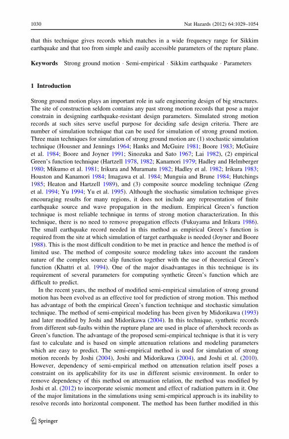
The state of Sikkim in north-eastern part of India was struck by a strong earthquake of

magnitude 6.9 (Mw) near the boundary between the Indian and Eurasian tectonic plates on

September 18, 2011. Parameters of this earthquake are given in Table 1. Sikkim Himalaya

is surrounded by three countries namely Nepal, China, and Bhutan. The shaking effects

88.00o88.25o 88.50o 88.75o 89.00o

27.00o

27.25o

27.50o

27.75o

28.00o

TISTALN

.

GA

NG

TOK

LN.

KANC

HENJU

NGA

F.LN

87.75o

STDS

STDS

LH

LH

Ductile thrust

Tethyan Sedimentary Sequence

Lesser Himalayan Rocks

Lineaments

Isograd boundary

LEGEND

MCT Zone

MCTZ

Fig. 1 Geological map of Sikkim Himalaya. MCTZ Main Central Thrust Zone, LH Lesser Himalaya, STDSSouth Tibetan Detachment System (Tectonic is taken from Nath et al. 2005 and geology is taken fromDasgupta et al. 2004)

Nat Hazards (2012) 64:1029–1054 1031

123

were more severe in eastern Nepal, which is closer to the epicenter. The earthquake was

felt most strongly in northern Bangladesh. In this region, the Indian plate converges with

Eurasian plate at a rate of approximately 5 cm/year toward the north–northeast (Tap-

ponnier and Molnar 1977). There are many transverse faults in the Sikkim region and

mainly two thrust faults in the south of the Sikkim region. Kayal (2001) has found the

seismic activity is mostly clustered in the north of the MBT where earthquake occurs at a

depth range 0–50 km.

In this region, entire Himalayan front is generally characterized by shallow-angle thrust

faulting. Most of the earthquakes in this region are predominantly strike-slip type and

occur along north-west trending Tista and Gangtok lineaments (Hazarika et al. 2010).

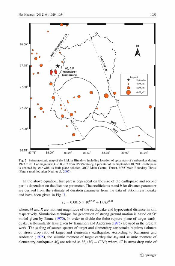
Figure 2 shows that the epicenter of Sikkim earthquake lies between Tista and Gangtok

lineaments. Distribution of past earthquakes in this region shown in Fig. 2 suggests that it

has experienced relatively moderate seismicity over past 38 years of magnitude [ 4 within

140 km radius of the epicenter of this magnitude earthquake.

2 Data and scaling laws

The Sikkim earthquake has been recorded by several strong motion stations in near-field as

well as far-field stations. This event has been recorded at near-field stations by the

Department of Earthquake Engineering, Indian Institute of Technology Roorkee, Utta-

rakhand. These stations have been installed in states of Himachal Pradesh, Punjab, Har-

yana, Rajasthan, Uttarakhand, Uttar Pradesh, Bihar, Sikkim, West Bengal, Meghalaya,

Arunachal Pradesh, Mizoram, Assam, and Andaman and Nicobar Islands. The Sikkim

earthquake of magnitude (Mw) 6.9 was recorded at nine station of this network at an

epicentral distance between 66 and 903 km. A very dense network of 14 stations has been

maintained by the Department of Earth Sciences, Indian Institute of Technology Roorkee

in the state of Uttarakhand. In this paper, acceleration records have been simulated at three

near-field source stations from network of entire Himalaya within the range of 200 km and

at twelve far-field stations within the epicentral distance of 900 km from the network of

Uttarakhand Himalaya. Generation of synthetic accelerogram for Sikkim earthquake using

semi-empirical approach requires various scaling laws. The semi-empirical technique of

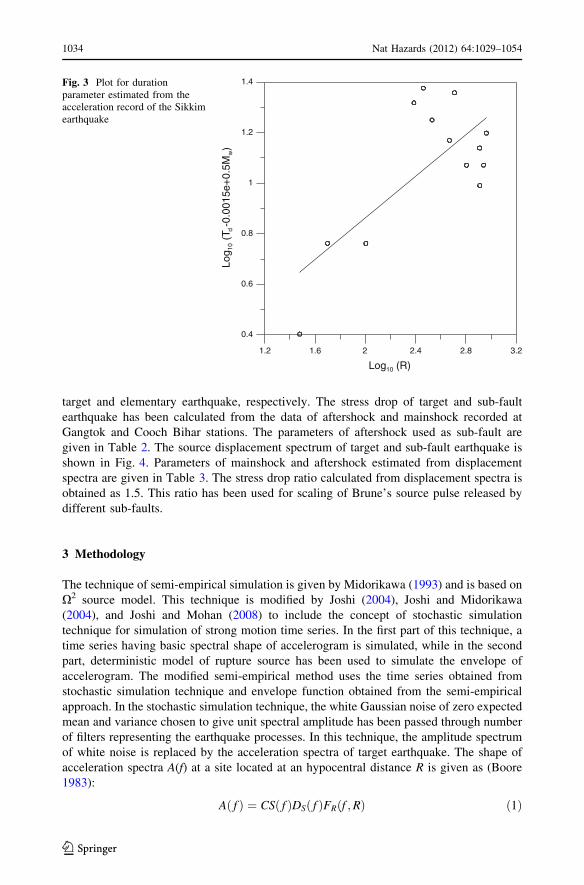
simulation of the envelope of accelerogram is dependent on the duration parameter. The

duration parameter can be estimated from recorded accelerogram in the source region, and

the regression relation for duration parameter is given by Midorikawa (1989) as:

Td ¼ 0:0015� 100:5M þ aRb

Table 1 Parameters of September 18, 2011 Sikkim earthquake, India

Hypocenter Size Fault plane solution Reference

12:41:02 s UTC27.43�N 88.33�E47.4 km

M0 = 2.78 9 1026 dyne cmMw = 6.9

NP1 u = 313�, d = 73�, k = -163�NP2 u = 217�, d = 74�, k = -18�

Global CMT

12:41:18 s UTC27.74�N 88.11�E35 km

M0 = 2.7 9 1026 dyne cmMw = 6.9

NP1 u = 220�, d = 78�, k = 0�NP2 u = 130�, d = 90�, k = 168�

USGS

1032 Nat Hazards (2012) 64:1029–1054

123

In the above equation, first part is dependent on the size of the earthquake and second

part is dependent on the distance parameter. The coefficients a and b for distance parameter

are derived from the estimate of duration parameter from the data of Sikkim earthquake

and have been given in Fig. 3.

Td ¼ 0:0015� 100:5M þ 1:08R0:41

where, M and R are moment magnitude of the earthquake and hypocentral distance in km,

respectively. Simulation technique for generation of strong ground motion is based on X2

model given by Brune (1970). In order to divide the finite rupture plane of target earth-

quake, self-similarity laws given by Kanamori and Anderson (1975) are used in the present

work. The scaling of source spectra of target and elementary earthquake requires estimate

of stress drop ratio of target and elementary earthquake. According to Kanamori and

Anderson (1975), the seismic moment of target earthquake M0 and seismic moment of

elementary earthquake M00 are related as M0

�M00 ¼ C0N3; where, C0 is stress drop ratio of

88.00o88.25o 88.50o 88.75o 89.00o 89.25o

26.75o

27.00o

27.25o

27.50o

27.75o

28.00o

MBT

MCT

TISTALN

.

GA

NG

TOK

LN.

KANC

HENJ

UNGA

F.LN

LegendEpicenter

4≤Mw<5

5≤Mw<6

6≤Mw<7

87.75o

Mw 6.918/09/2011Mainshock

Fig. 2 Seismotectonic map of the Sikkim Himalaya including location of epicenters of earthquakes during1973 to 2011 of magnitude 4 \ M \ 7 from USGS catalog. Epicenter of the September 18, 2011 earthquakeis denoted by star with its fault plane solution. MCT Main Central Thrust, MBT Main Boundary Thrust(Figure modified after Nath et al. 2005)

Nat Hazards (2012) 64:1029–1054 1033

123

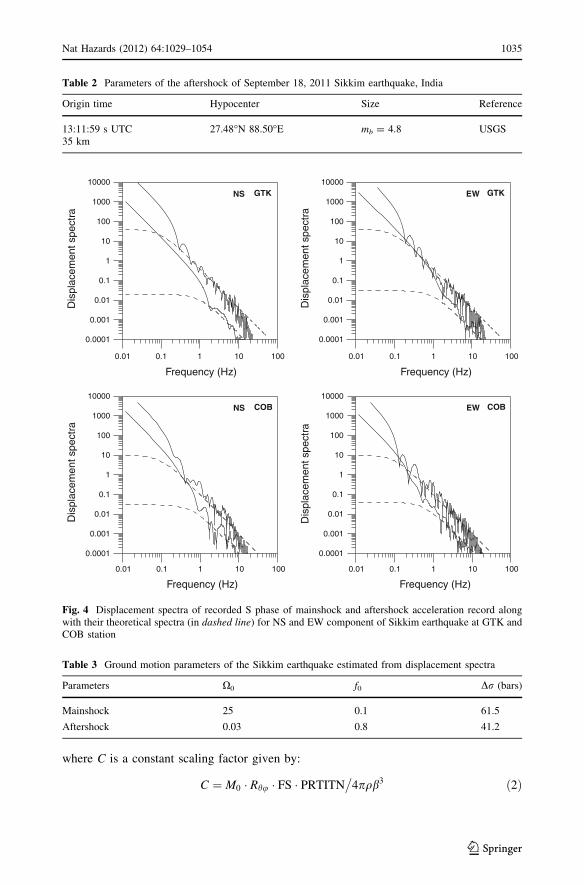
target and elementary earthquake, respectively. The stress drop of target and sub-fault

earthquake has been calculated from the data of aftershock and mainshock recorded at

Gangtok and Cooch Bihar stations. The parameters of aftershock used as sub-fault are

given in Table 2. The source displacement spectrum of target and sub-fault earthquake is

shown in Fig. 4. Parameters of mainshock and aftershock estimated from displacement

spectra are given in Table 3. The stress drop ratio calculated from displacement spectra is

obtained as 1.5. This ratio has been used for scaling of Brune’s source pulse released by

different sub-faults.

3 Methodology

The technique of semi-empirical simulation is given by Midorikawa (1993) and is based on

X2 source model. This technique is modified by Joshi (2004), Joshi and Midorikawa

(2004), and Joshi and Mohan (2008) to include the concept of stochastic simulation

technique for simulation of strong motion time series. In the first part of this technique, a

time series having basic spectral shape of accelerogram is simulated, while in the second

part, deterministic model of rupture source has been used to simulate the envelope of

accelerogram. The modified semi-empirical method uses the time series obtained from

stochastic simulation technique and envelope function obtained from the semi-empirical

approach. In the stochastic simulation technique, the white Gaussian noise of zero expected

mean and variance chosen to give unit spectral amplitude has been passed through number

of filters representing the earthquake processes. In this technique, the amplitude spectrum

of white noise is replaced by the acceleration spectra of target earthquake. The shape of

acceleration spectra A(f) at a site located at an hypocentral distance R is given as (Boore

1983):

A fð Þ ¼ CS fð ÞDS fð ÞFR f ;Rð Þ ð1Þ

1.2 1.6 2 2.4 2.8 3.2

Log10 (R)

0.4

0.6

0.8

1

1.2

1.4

Log 1

0 (T

d-0

.001

5e+

0.5M

w)

Fig. 3 Plot for durationparameter estimated from theacceleration record of the Sikkimearthquake

1034 Nat Hazards (2012) 64:1029–1054

123

where C is a constant scaling factor given by:

C ¼ M0 � Rhu � FS � PRTITN�

4pqb3 ð2Þ

Frequency (Hz)

0.0001

0.001

0.01

0.1

1

10

100

1000

10000

Dis

plac

emen

t spe

ctra

NS GTK

Frequency (Hz)

0.0001

0.001

0.01

0.1

1

10

100

1000

10000

Dis

plac

emen

t spe

ctra

EW GTK

Frequency (Hz)

0.0001

0.001

0.01

0.1

1

10

100

1000

10000

Dis

plac

emen

t spe

ctra

NS COB

0.01 0.1 1 10 100

0.01 0.1 1 10 1000.01 0.1 1 10 100

0.01 0.1 1 10 100

Frequency (Hz)

0.0001

0.001

0.01

0.1

1

10

100

1000

10000

Dis

plac

emen

t spe

ctra

EW COB

Fig. 4 Displacement spectra of recorded S phase of mainshock and aftershock acceleration record alongwith their theoretical spectra (in dashed line) for NS and EW component of Sikkim earthquake at GTK andCOB station

Table 3 Ground motion parameters of the Sikkim earthquake estimated from displacement spectra

Parameters X0 f0 Dr (bars)

Mainshock 25 0.1 61.5

Aftershock 0.03 0.8 41.2

Table 2 Parameters of the aftershock of September 18, 2011 Sikkim earthquake, India

Origin time Hypocenter Size Reference

13:11:59 s UTC35 km

27.48�N 88.50�E mb = 4.8 USGS

Nat Hazards (2012) 64:1029–1054 1035

123

In this expression, M0 is the seismic moment, Rhu is the radiation pattern, FS is the

amplification due to the free surface, PRTITN is the reduction factor that accounts for the

partitioning of total shear wave energy into two horizontal components (taken as 1/H2),

and q and b are the density and shear velocity, respectively. The radiation pattern Rhu is

dependent on the type of faulting mechanism and the geometry of earthquake source. The

filter S(f) in Eq. (1) is the source acceleration spectrum which is defined by Brune (1970) as

follows:

S fð Þ ¼ 2pfð Þ2.

1þ f=fcð Þ2h i

ð3Þ

In Eq. (1), filter DS(f) is the near-site attenuation of high frequencies and is defined as

(Boore 1983):

DS fð Þ ¼ 1.

1þ f=fmð Þ8h i1=2

ð4Þ

The parameter fm represents the high frequency cutoff range of the high-cut filter. The

filter FR(f, R) represents the effect of anelastic attenuation and is given as (Boore 1983):

FR f ;Rð Þ ¼ e�pfR=bQb fð Þ� �.

R ð5Þ

where R denotes the hypocentral distance in km and Qb(f) is the quality factor which

defines the frequency-dependent attenuation during the wave propagation. In the present

work, the frequency-dependent quality factor Qb(f) for Sikkim region is used as

Qb(f) = 167f0.47 (Nath and Thingbaijam 2009).

The spectrum of white noise after multiplication with theoretical filters given in Eq. (1)

represents basic shape of acceleration spectra. Time domain representation of this accel-

eration spectrum gives an acceleration record that has basic properties of acceleration

spectra. However, this time domain representation of acceleration record raises serious

problem, like the obtained records overestimate the high frequency strong ground motion

and underestimate low frequency in the synthetic strong ground motion. This is due to the

difference in duration of slip of the target and the small earthquake considered as sub-

faults. The difference in the duration of slip of the target and the sub-fault earthquake

following correction function F(t) given by Irikura et al. (1997) and Irikura and Kamae

(1994) is corrected by convolving with the obtained acceleration records:

F tð Þ ¼ d tð Þ þ ðN � 1Þ=TRð1� expð�1ÞÞ½ � � expð�t=TRÞ ð6Þ

where d(t) is the delta function, N is the total number of sub-faults along the length or the

width of the rupture plane, and TR is the rise time of the target earthquake. The convolution

of F(t) with obtained acceleration record aij(t) gives acceleration record Aij(t) as:

Aij tð Þ ¼ F tð Þ � aij tð Þ ð7Þ

where i and j represent the position of sub-fault along the length and the width of the

rupture plane, respectively. It is observed that stochastic simulation technique requires

proper windowing of the obtained record by a function which is based on kinematic

representation of model of rupture (Boore 1983). Such time window can be obtained by the

semi-empirical technique of Midorikawa (1993) in the form of resultant envelope of ac-

celerogram obtained from a model of finite rupture plane. The finite fault in the semi-

empirical technique proposed by Midorikawa (1993) is divided into several sub-faults is

based on self-similarity laws proposed by Kanamori and Anderson (1975). Energy is

1036 Nat Hazards (2012) 64:1029–1054

123

released in the form of acceleration envelop whenever rupture approaches center of ele-

ments. The acceleration envelope waveform eij(t) is determined from the following

functional form given by Kameda and Sugito (1978) and further modified by Joshi (2004):

eij tð Þ ¼ Tss t=Tdð Þ � exp 1� t=Tdð Þ ð8Þ

In this expression, Td represents duration parameter and Tss represents the transmission

coefficient of incident shear waves. This coefficient is given by the following formula after

Lay and Wallace (1995, p. 102) and is used by Joshi et al. (2001) for modeling the effect of

the transmission of energy in the shape of acceleration envelope as:

Tss ¼ 2l2gb2

.l1gb1

þ l2gb2

� �ð9Þ

where l1 and l2 are modulus of rigidity in the first and second layers, respectively, and b1

and b2 are shear wave velocities in the first and second layers, respectively. The trans-

mission coefficient contributes significantly to shaping the attenuation rate of the peak

ground acceleration with respect to the distance from the source. Joshi and Midorikawa

(2004) have observed that for the shallow focus earthquakes, the transmission coefficient is

&1.0; however, for the intermediate to deep focus earthquake, this coefficient is =1.0.

This means that we should take this coefficient into consideration when modeling an

intermediate to deep focus earthquake.

The parameters required to define the model of the rupture plane are its length (L), width

(W), length and width of the sub-faults (Le, We), nucleation point, strike and dip of rupture

plane (us, d), rupture velocity (Vr) and shear wave velocity in the medium. The rectangular

rupture plane of a target earthquake of seismic moment M0 is divided into N 9 N sub-

faults of seismic moment M00: Once the rupture plane of target earthquake is divided into

sub-faults, one sub-fault is fixed as nucleation point from which the rupture initiates. This

point can coincide with the focus of the earthquake. The rupture starts from the nucleation

point and propagates radially within the rupture plane. The sub-fault releases energy

whenever the rupture front touches its center. The energy is released in the form of

acceleration record acij(t), which is the product of acceleration record from stochastic

technique with envelope function from semi-empirical simulation technique as:

acij tð Þ ¼ eij tð Þ � Aij tð Þ ð10Þ

The acceleration record, acij(t), released from different sub-faults reaches the obser-

vation point at different time. The arrival time at the observation point tij depends on the

time taken by rupture from nucleation point to ijth sub-fault with rupture velocity Vr and

time taken by energy released from ijth sub-fault to reach the observation point with

velocity V of propagation. The total time taken tij is given as (Joshi and Midorikawa 2004):

tij ¼ rij

�V þ nij

�Vr ð11Þ

where rij is the distance from the observation point to the ijth sub-fault and nij is the

distance travelled by the rupture from nucleation point to particular sub-fault.

In the present work, simple vector notation has been used to resolve these resultant

components into horizontal components. The direction of resultant component from each

sub-fault is defined by a line joining center of sub-fault to the recording station. This

direction is different for different sub-faults and for obtaining horizontal component along

strike and perpendicular direction of the modeled rupture plane, records from each sub-

faults need separate treatment. Figure 5 shows the division of total acceleration record

Nat Hazards (2012) 64:1029–1054 1037

123

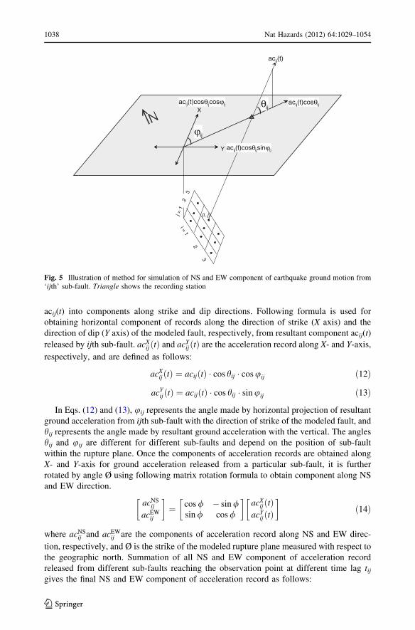
acij(t) into components along strike and dip directions. Following formula is used for

obtaining horizontal component of records along the direction of strike (X axis) and the

direction of dip (Y axis) of the modeled fault, respectively, from resultant component acij(t)

released by ijth sub-fault. acXij ðtÞ and acY

ijðtÞ are the acceleration record along X- and Y-axis,

respectively, and are defined as follows:

acXij ðtÞ ¼ acijðtÞ � cos hij � cos uij ð12Þ

acYijðtÞ ¼ acijðtÞ � cos hij � sin uij ð13Þ

In Eqs. (12) and (13), uij represents the angle made by horizontal projection of resultant

ground acceleration from ijth sub-fault with the direction of strike of the modeled fault, and

hij represents the angle made by resultant ground acceleration with the vertical. The angles

hij and uij are different for different sub-faults and depend on the position of sub-fault

within the rupture plane. Once the components of acceleration records are obtained along

X- and Y-axis for ground acceleration released from a particular sub-fault, it is further

rotated by angle Ø using following matrix rotation formula to obtain component along NS

and EW direction.

acNSij

acEWij

� �¼ cos / � sin /

sin / cos /

� �acX

ij tð ÞacY

ij tð Þ

� �ð14Þ

where acNSij and acEW

ij are the components of acceleration record along NS and EW direc-

tion, respectively, and Ø is the strike of the modeled rupture plane measured with respect to

the geographic north. Summation of all NS and EW component of acceleration record

released from different sub-faults reaching the observation point at different time lag tijgives the final NS and EW component of acceleration record as follows:

acij(t)

)

i =1

2

3(i, j)j =

12

3

X

Y

acij(t)cosθijacij(t)cosθijcosϕij

ϕij

acij(t)cosθijsinϕij

θij

)

Fig. 5 Illustration of method for simulation of NS and EW component of earthquake ground motion from‘ijth’ sub-fault. Triangle shows the recording station

1038 Nat Hazards (2012) 64:1029–1054

123

AcNS tð Þ ¼XN

i¼1

XN

j¼1

acNSij t � tij

� �ð15Þ

AcEW tð Þ ¼XN

i¼1

XN

j¼1

acEWij t � tij

� �ð16Þ

where AcNS tð Þ and AcEW tð Þ represent the north–south and east–west component of

acceleration records, respectively. A FORTRAN code, named MSETCS (Modified Semi

Empirical Technique for Component-wise Simulation) has been developed using the

proposed method for component wise simulation of strong ground motion.

4 Methodology: a discussion

Directivity effects are considered to be one of the most important properties of strong motion

records. The approach of semi-empirical modeling given by Midorikawa (1993) clearly

Distance (Km)

-400

-200

0

200

400

Dis

tanc

e (K

m)

-1000 -500 0 500 1000 1500

-1000 -500 0 500 1000 1500

Distance (Km)

-400

-200

0

200

400

Dis

tanc

e (K

m)

(a)

(b)

A B

A B

. .

. .

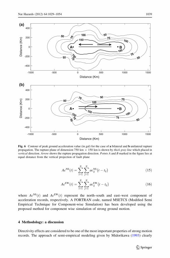
Fig. 6 Contour of peak ground acceleration value (in gal) for the case of a bilateral and b unilateral rupturepropagation. The rupture plane of dimension 750 km 9 150 km is shown by thick gray line which placed invertical direction. Arrow shows the rupture propagation direction. Points A and B marked in the figure lies atequal distance from the vertical projection of fault plane

Nat Hazards (2012) 64:1029–1054 1039

123

follows directivity effects. The modifications in the semi-empirical approach suggested by

Joshi and Midorikawa (2004) for layering and correction function also confirm the presence

of directivity effects in the simulated records. In the present work, seismic moment has been

used for scaling the amplitude of accelerogram together with the radiation pattern. These

modifications require an investigation regarding applicability of directivity effects in strong

motion records. In order to check the effect of directivity in the modified technique, strong

motion records are simulated on both sides of the rupture plane for bilateral and unilateral

rupture propagations. In this numerical experiment, a simple vertical rupture plane of length

750 km and downward extension 150 km has been assumed. The dip and rake of this rupture

is assumed to be 90� and 0� to consider pure strike-slip mechanism. This rupture plane is

divided into 81 sub-faults, each of which corresponds to 7.1 (Mw) magnitudes and placed in a

layered velocity model defined by Cotte et al. (1999). Variation of peak ground acceleration

on both sides of the rupture plane in strike direction for bilateral rupture propagation and

unilateral rupture propagation is shown in Fig. 6. It is observed that due to inclusion of

radiation pattern, transmission effect, and component wise simulation, absolute symmetry is

not obtained in case of bilateral rupture propagation. However, it is observed that two points

equidistant from the corner of rupture plane have nearly same peak ground acceleration for

bilateral propagation. In case of unilateral rupture propagation, peak ground acceleration

values are higher in the direction of rupture propagation compared to peak ground accel-

eration in the opposite direction of rupture propagation. This confirms the presence of

directivity effect in the modified technique which is used for component wise simulation of

strong ground motion in this paper.

5 Rupture model of Sikkim earthquake

Location of the causative fault of this earthquake is decided on the basis of location of

epicenter of this earthquake and seismic activity in the region. Most of the earthquakes in

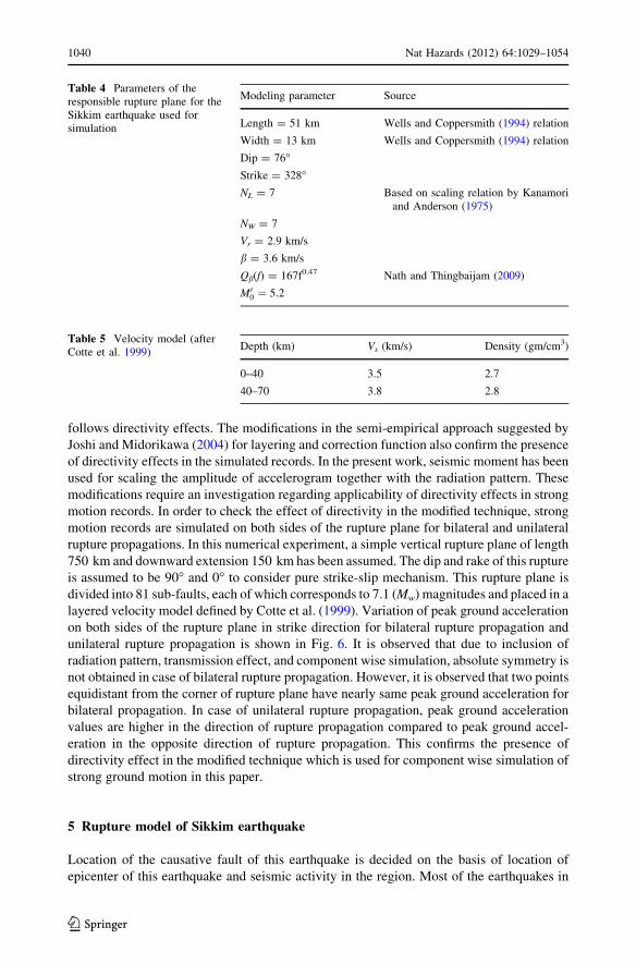
Table 4 Parameters of theresponsible rupture plane for theSikkim earthquake used forsimulation

Modeling parameter Source

Length = 51 km Wells and Coppersmith (1994) relation

Width = 13 km Wells and Coppersmith (1994) relation

Dip = 76�Strike = 328�NL = 7 Based on scaling relation by Kanamori

and Anderson (1975)

NW = 7

Vr = 2.9 km/s

b = 3.6 km/s

Qb(f) = 167f0.47 Nath and Thingbaijam (2009)

M00 ¼ 5:2

Table 5 Velocity model (afterCotte et al. 1999)

Depth (km) Vs (km/s) Density (gm/cm3)

0–40 3.5 2.7

40–70 3.8 2.8

1040 Nat Hazards (2012) 64:1029–1054

123

this region are predominantly strike-slip type and occur along north-west trending Tista

and Gangtok lineaments (Hazarika et al. 2010). The rupture responsible for this earthquake

is placed at a depth of 44 km between Tista and Gangtok lineaments. The rupture length

and width of the Sikkim earthquake has been calculated using the relation given by Wells

and Coppersmith (1994). This gives the length and width of rupture plane as 51 and 13 km,

respectively. The strike of rupture plane is assumed as parallel to Tista lineament as 328�N

which is close to that obtained from fault plane solution of this earthquake given by CMT

Harvard. The seismic moment of the aftershock of the Sikkim earthquake used for com-

puting stress drop is 7.9 9 1023 dyne cm (calculated from displacement spectra), which

Table 6 Details of the near-field strong motion recording stations which has recorded the Sikkimearthquake

Station name Latitude(in degree)

Longitude(in degree)

Station code Hypocentraldistance (km)

Gangtok 27.352 88.627 GTK 81.84

Siliguri 26.712 88.428 SLG 127.59

Cooch Bihar 26.319 89.440 COB 210.98

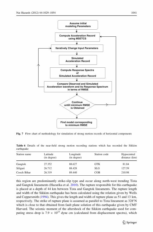
Assume initial modeling Parameters

Compare Observed and Simulated Acceleration waveform and its Response Spectrum

in terms of RMSE

Find model corresponding to minimum RMSE

Simulated Acceleration Record

Continue untill minimum RMSE

is Obtained

Compute Acceleration Recordusing MSETCS

Iteratively Change Input Parameters

Compute Response Spectra of

Simulated Acceleration Record

Fig. 7 Flow chart of methodology for simulation of strong motion records of horizontal components

Nat Hazards (2012) 64:1029–1054 1041

123

further used for dividing the rupture plane of the target earthquake. The rupture plane of

target earthquake has been divided into 7 9 7 sub-faults of magnitude 5.2 (Mw) on the

basis of self-similarity law given by Kanamori and Anderson (1975). Parameters of the

rupture plane responsible for the Sikkim earthquake used for simulation are listed in

Table 4. The velocity model used for simulation of ground motion at different sites is that

given by Cotte et al. (1999) and defined in Table 5. Density value used in the velocity

model has been decided on the basis of relation between P-wave velocity and density of

earth medium given by Brocher (2005). The rupture plane of the target earthquake is

placed in the second layer of velocity model at a depth of 44 km. The parameters of final

88.00o 88.25o 88.50o 88.75o 89.00o 89.25o

26.75o

27.00o

27.25o

27.50o

27.75o

28.00o

MBT

MCT

TISTALN

.

GA

NG

TOK

LN.

KAN

CHEN

JUNG

AF.

LN

LEGEND

Strong Motion Station

GTK

SLG

COB

87.75o 89.50o

26.50o

26.25o

Fig. 8 Location of the fault rupture plane responsible for Sikkim earthquake of magnitude (Mw) 6.9.Triangles show the position of strong motion stations. MCT Main Central Thrust, MBT Main BoundaryThrust (Figure modified after Nath et al. 2005)

1042 Nat Hazards (2012) 64:1029–1054

123

rupture model are decided on the basis of quantitative comparison of observed and sim-

ulated acceleration waveform in terms of root mean square error. For the calculation of

root mean square error between simulated and observed record, following formula given

by Joshi and Midorikawa (2004) has been used:

PGA 59

PGA 59

PGA 59

PGA 62

PGA 63 PGA 70

PGA 82 PGA 158

PGA 156

PGA 157

0 45 90

-200

0

200 PGA 158

RMSE 0.48

25.0ESMR65.0ESMR16.0ESMR RMSE 0.49

PGA 61 PGA 61 PGA 81

25.0ESMR75.0ESMR65.0ESMR

PGA 62 PGA 62 PGA 65

45.0ESMR75.0ESMR65.0ESMR

RMSE 0.61 RMSE 0.56

RMSE 0.61

RMSE 0.52

RMSE 0.49

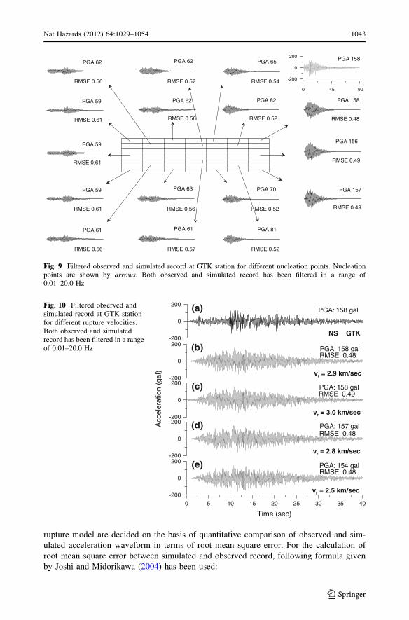
Fig. 9 Filtered observed and simulated record at GTK station for different nucleation points. Nucleationpoints are shown by arrows. Both observed and simulated record has been filtered in a range of0.01–20.0 Hz

NS

PGA: 158 gal

GTK-200

0

200

Acc

eler

atio

n (g

al)

PGA: 158 gal

vr = 2.9 km/sec-200

0

200

PGA: 154 gal

0 5 10 15 20 25 30 35 40

Time (sec)

-200

0

200

PGA: 158 gal

-200

0

200

PGA: 157 gal

-200

0

200

(a)

(b)

(e)

(c)

(d)vr = 3.0 km/sec

vr = 2.8 km/sec

vr = 2.5 km/sec

RMSE 0.48

RMSE 0.48

RMSE 0.49

RMSE 0.48

Fig. 10 Filtered observed andsimulated record at GTK stationfor different rupture velocities.Both observed and simulatedrecord has been filtered in a rangeof 0.01–20.0 Hz

Nat Hazards (2012) 64:1029–1054 1043

123

NS

PGA: 158 gal

GTK-200

0

200

Acc

eler

atio

n (g

al)

PGA: 158.4

δ = 76 -200

0

200

PGA: 158.8

-200

0

200

PGA: 158.5

-200

0

200

PGA: 158.7

-200

0

200

(a)

(b)

(e)

(c)

(d)

RMSE 0.49

RMSE 0.49

RMSE 0.49

RMSE 0.48

PGA: 158.9

0 5 10 15 20 25 30 35 40

Time (sec)

-200

0

200(f)

RMSE 0.49

δ = 75

δ = 74

δ = 73

δ = 72

Fig. 11 Filtered observed andsimulated record at GTK stationfor different dip angle. Bothobserved and simulated recordhas been filtered in a range of0.01–20.0 Hz

N 3280

760 DipV1= 3.5 km/s

V2= 3.8 km/s

Surface projection

Fig. 12 Source model of the Sikkim earthquake consisting 7 9 7 sub-faults placed in a layered mediumwith 328�N strike direction. Solid circle shows the starting position of rupture

1044 Nat Hazards (2012) 64:1029–1054

123

MCT

SAT

Ramgarh NAT

Moradabad Fault

Fault

MBT

Martoli

Thrust

Kali

Riv

er

NEPAL

BHUTAN

TIBET

78o 80o 82o84o 86o 88o 90o 92o

24o

26o

28o

30o

32o

LEGEND

Epicenter (USGS)DEQ Strong Motion StationsKumaon Strong Motion Stations

80o 81o79o

29o

30o

CMO

UDH

CHP

BHAG BERI

MUAV

PITH

BALJAUL

Ophiolite/ Melange

Crystalline complex overprinted byHimalayan fold- thrust movement

Older folded cover sequenceoverprinted by Himalayanfold- thrust movement

Older cover sequence folded during Himalayan fold- thrust movement

Thrust

Location of stations of Kumaonstrong motion network

Minor Lineament

Fault

LEGEND

Location of stations of DEQ strong motion network

88.00o 88.25 o 88.50o 88.75o 89.00o 89.25o

26.75o

27.00o

27.25o

27.50o

27.75o

28.00o

LEGEND

Epicenter LocationStrong Motion Station

GTK

SLG

COBKOK

87.75o 89.50o

26.50o

26.25o

89.75 o 90.00o 90.25o 90.50o

RAX

MLD

BHUTAN

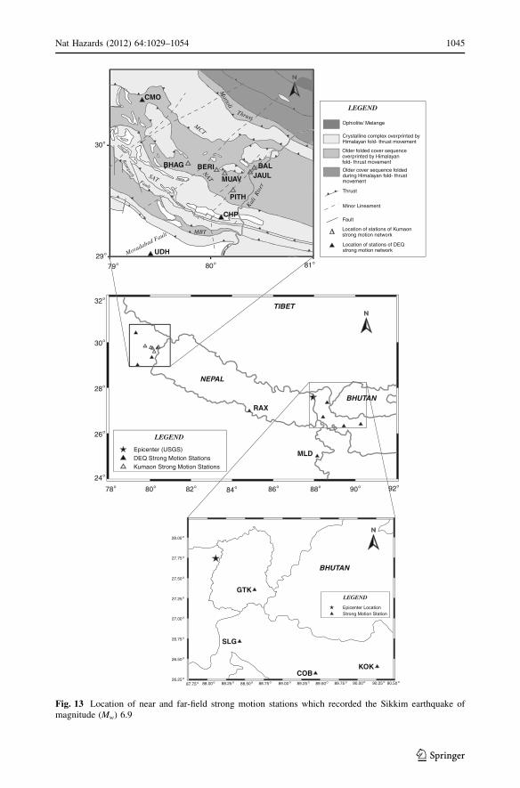
Fig. 13 Location of near and far-field strong motion stations which recorded the Sikkim earthquake ofmagnitude (Mw) 6.9

Nat Hazards (2012) 64:1029–1054 1045

123

RMSE ¼ 1=N �XN

i¼1

af ið Þ � as ið Þas ið Þ

2" #1=2

ð17Þ

where RMSE is root mean square error of N samples of observed af(i) and simulated as(i)records. The flow graph showing procedure of iterative modeling is shown in Fig. 7.

30 35 40 45 50 55 60 65 70

Time (sec)

-200

-100

0

100

200

NS

PGA: 158 gal

GTK

30 35 40 45 50 55 60 65 70

Time (sec)

-200

-100

0

100

200

Acc

eler

atio

n (g

al)

EW

PGA: 149 gal

GTK

NS

PGA: 158 gal

GTK

0 5 10 15 20 25 30 35 40

Time (sec)

-200

-100

0

100

200

Acc

eler

atio

n (g

al)

EW

PGA: 136 gal

GTK

50 55 60 65 70 75 80 85 90

Time (sec)

-200

-100

0

100

200

NS

PGA: 58 gal

COB

50 55 60 65 70 75 80 85 90

Time (sec)

-200

-100

0

100

200

Acc

eler

atio

n (g

al)

EW

PGA: 44 gal

COB

0 5 10 15 20 25 30 35 40

Time (sec)

-200

-100

0

100

200

NS

PGA: 129 gal

COB

0 5 10 15 20 25 30 35 40

Time (sec)

-200

-100

0

100

200

Acc

eler

atio

n (g

al)

EW

PGA: 99 gal

COB

25 30 35 40 45 50 55 60 65

Time (sec)

-200

-100

0

100

200

NS

PGA: 201 gal

SLG

25 30 35 40 45 50 55 60 65

Time (sec)

-200

-100

0

100

200

Acc

eler

atio

n (g

al)

EW

PGA: 156 gal

SLG

0 5 10 15 20 25 30 35 40

Time (sec)

-200

-100

0

100

200

NS

PGA: 246 gal

SLG

0 5 10 15 20 25 30 35 40

Time (sec)

-200

-100

0

100

200

Acc

eler

atio

n (g

al)

EW

PGA: 169 gal

SLG

0 5 10 15 20 25 30 35 40

Time (sec)

-200

-100

0

100

200

(a) (b)Obs.

Syn.

Obs.

Syn.

Obs.

Syn.

Obs.

Syn.

Obs.

Syn.

Obs.

Syn.

(c) (d)

(i) (j)

(k) (l)

(e) (f)

(g) (h)

Fig. 14 Comparisons of observed and simulated acceleration record of NS and EW component for Sikkimearthquake of magnitude (Mw) 6.9 at near stations

1046 Nat Hazards (2012) 64:1029–1054

123

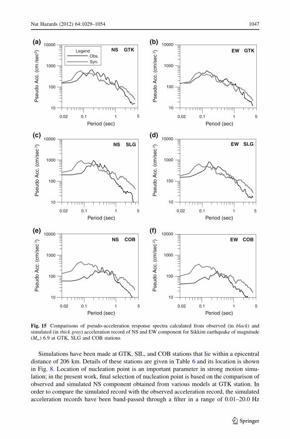
Simulations have been made at GTK, SIL, and COB stations that lie within a epicentral

distance of 206 km. Details of these stations are given in Table 6 and its location is shown

in Fig. 8. Location of nucleation point is an important parameter in strong motion simu-

lation; in the present work, final selection of nucleation point is based on the comparison of

observed and simulated NS component obtained from various models at GTK station. In

order to compare the simulated record with the observed acceleration record, the simulated

acceleration records have been band-passed through a filter in a range of 0.01–20.0 Hz

0.1 1

Period (sec)

10

100

1000

10000

Pse

udo

Acc

. (cm

/sec

2 ) LegendObs.Syn.

NS GTK

0.1 1

Period (sec)

10

100

1000

10000

Pse

udo

Acc

. (cm

/sec

2 ) EW GTK

(a) (b)

0.1 1

Period (sec)

10

100

1000

10000

Pse

udo

Acc

. (cm

/sec

2 ) NS COB

0.1 1

Period (sec)

10

100

1000

10000

Pse

udo

Acc

. (cm

/sec

2 ) EW COB

(e) (f)

0.1 1

Period (sec)

10

100

1000

10000

Pse

udo

Acc

. (cm

/sec

2 ) NS SLG

0.1 1

Period (sec)

10

100

1000

10000

Pse

udo

Acc

. (cm

/sec

2 ) EW SLG

(c) (d)

50.0250.02

50.02 50.02

50.02 50.02

Fig. 15 Comparisons of pseudo-acceleration response spectra calculated from observed (in black) andsimulated (in thick gray) acceleration record of NS and EW component for Sikkim earthquake of magnitude(Mw) 6.9 at GTK, SLG and COB stations

Nat Hazards (2012) 64:1029–1054 1047

123

which is used for the processing of observed acceleration record at different stations. Root

mean square error between observed and simulated waveform has been calculated for each

cases. Various simulated records and its comparison with observed record in terms of root

mean square error for different possibilities of nucleation point are shown in Fig. 9. The

comparison in terms of root mean square error suggests location of the nucleation point in

the extreme north-west corner of rupture plane at a depth of 47 km and has been retained

for further use. In all models used for selecting nucleation point, rupture velocity and dip

angle have been assumed as 2.9 km/s and 14�, respectively. The effect of rupture velocity

and the dip angle in the rupture model has been checked in the present work. Various

rupture velocity ranging from 2.5 to 3.0 km/s have been considered for simulating NS

component of acceleration record at GTK station. Figure 10 shows the comparison of

observed and simulated acceleration record for considering rupture velocity 2.5, 2.8, 2.9,

and 3.0 km/s. Based on minimum root mean square error, rupture velocity 2.9 km/s has

been used as final rupture velocity for further simulations. In order to check the depen-

dency of dip angle in the simulation, rupture model has been tested on few dip angles

ranging from 72� to 76�. From Fig. 11, it is observed that there is no drastic change in the

peak ground acceleration parameter and in the root mean square error. Based on this

observation, dip angle 76� has been used for simulation of ground motion of Sikkim

earthquake. Final rupture model of the Sikkim earthquake is shown in Fig. 12.

6 Near-field simulation of strong motion record

Acceleration records have been simulated at three near-field stations using final rupture

parameters given in Table 4. Location of near-field and far-field strong motion stations is

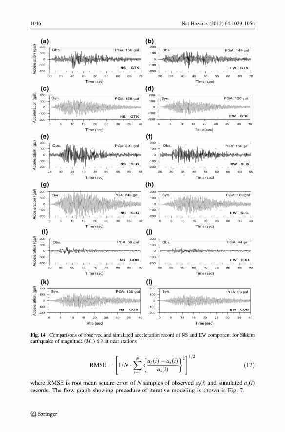
shown in Fig. 13. Comparison of observed and simulated acceleration record at GTK,

SLG, and COB stations is shown in Fig. 14, and it shows that simulated record bears

realistic shape as that of observed record and the peak ground acceleration of observed and

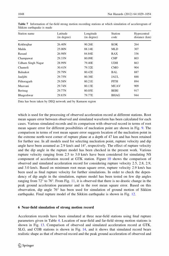
Table 7 Information of far-field strong motion recording stations at which simulation of accelerogram ofSikkim earthquake is made

Station name Latitude(in degree)

Longitude(in degree)

Stationcode

Hypocentraldistance (km)

Kokhrajhar 26.40N 90.26E KOK 264

Malda 25.00N 88.14E MLD 307

Raxaul 26.98N 84.84E RAX 336

Champawat 29.33N 80.09E CHP 803

Udham Singh Nagar 28.99N 79.40E UDH 863

Chamoli 30.41N 79.32E CMO 904

Baluakot 29.79N 80.42E BAL 887

Jauljibi 29.75N 80.38E JAUL 888

Pithoragarh 29.58N 80.21E PITH 894

Muavani 29.74N 80.13E MUAV 909

Berinag 29.77N 80.05E BERI 917

Bhageshwar 29.83N 79.77E BHAG 944

Data has been taken by DEQ network and by Kumaon region

1048 Nat Hazards (2012) 64:1029–1054

123

simulated record is also comparable. Pseudo-acceleration response spectra at 5 % damping

have been generated from observed and simulated acceleration record and are compared in

Fig. 15. Comparisons of response spectrum suggest the both simulated and observed

response spectra give a comparable match in the response spectra at all near-field stations.

This confirms the suitability of the model and its selected parameters for generation of

strong ground motion for both NS and EW components.

0 50 100

-3

0

3

0 50 100

-3

0

3-3

0

3

-3

0

3

NS BAL

PGA= 2

EW BAL

PGA= 2.8

2.2=AGP4.2=AGP

0 50 100

-3

0

3

0 50 100

-3

0

3-3

0

3

-3

0

3

NS JAUL

PGA= 1.8

EW JAUL

PGA= 2.5

PGA= 2.3 PGA= 2.1

0 50 100

-3

0

3

0 50 100

-3

0

3-3

0

3

-3

0

3

NS PITH

PGA= 3

EW PITH

PGA= 3

PGA= 2 PGA= 1.8

0 50 100

-3

0

3

0 50 100

-3

0

3-3

0

3

-3

0

3

NS MUAV

PGA= 1.7

EW MUAV

PGA= 1.3

PGA= 2.5 PGA= 2

0 50 100Time (sec)

-3

0

3

0 50 100Time (sec)

-3

0

3-3

0

3

-3

0

3

NS BERI

PGA= 0.6

EW BERI

PGA= 0.7

PGA= 2.1 PGA= 1.9

0 50 100Time (sec)

-3

0

3

0 50 100Time (sec)

-3

0

3-3

0

3

-3

0

3

NS BHAG

PGA= 1.3

EW BHAG

PGA= 1.5

PGA= 2 PGA= 1.8

Acc

eler

atio

n (g

al)

Acc

eler

atio

n (g

al)

Acc

eler

atio

n (g

al)

Acc

eler

atio

n (g

al)

Acc

eler

atio

n (g

al)

Acc

eler

atio

n (g

al)

0 20 40 60 80

-100

0

100

0 20 40 60 80

-100

0

100-100

0

100

-100

0

100

NS KOK

PGA= 52

EW KOK

PGA= 43

PGA= 58 PGA= 35

0 20 40 60 80

-40

0

40

0 20 40 60 80

-40

0

40-40

0

40

-40

0

40

NS MLD

PGA= 23

EW MLD

PGA= 23

PGA= 24 PGA= 19

0 20 40 60 80

-40

0

40

0 20 40 60 80

-40

0

40-40

0

40

-40

0

40

NS RAX

PGA= 27

EW RAX

PGA= 20

23=AGP6=AGP

0 20 40 60 80

-3

0

3

0 20 40 60 80

-3

0

3-3

0

3

-3

0

3

NS CHP

PGA= 2

EW CHP

PGA= 2

PGA= 0.5 PGA= 0.7

0 20 40 60 80

Time (sec)

-3

0

3

0 20 40 60 80

Time (sec)

-3

0

3-3

0

3

-3

0

3

NS UDH

PGA= 2

EW UDH

PGA= 2

5.1=AGP1=AGP

0 20 40 60 80

Time (sec)

-3

0

3

0 20 40 60 80

Time (sec)

-3

0

3-3

0

3

-3

0

3

NS CMO

PGA= 2

EW CMO

PGA= 1

PGA= 0.7 PGA= 0.8

Acc

eler

atio

n (g

al)

Acc

eler

atio

n (g

al)

Acc

eler

atio

n (g

al)

Acc

eler

atio

n (g

al)

Acc

eler

atio

n (g

al)

Acc

eler

atio

n (g

al)

Fig. 16 Comparison of NS and EW component of observed and simulated acceleration record at differentstrong motion stations which placed at an epicentral distance of 260–903 km range. Station codes and peakground acceleration values for observed (in black) and simulated (in gray) acceleration record are indicatedin different plot

Nat Hazards (2012) 64:1029–1054 1049

123

7 Far-field simulation of strong motion record

Simulations using the same rupture model have been made at twelve far-field stations.

These includes six station managed by the Department of Earthquake Engineering and six

0.1 1

Period (sec)

0.1

1

10

100

1000NS BAL

0.1 1

Period (sec)

0.1

1

10

100

1000EW BAL

0.1 1

Period (sec)

0.1

1

10

100

1000NS BERI

0.1 1

Period (sec)

0.1

1

10

100

1000EW BERI

0.1 1

Period (sec)

0.1

1

10

100

1000NS PITH

0.1 1

Period (sec)

0.1

1

10

100

1000EW PITH

0.1 1

Period (sec)

0.1

1

10

100

1000NS JAUL

0.1 1

Period (sec)

0.1

1

10

100

1000EW JAUL

0.1 1

Period (sec)

0.1

1

10

100

1000NS BHAG

0.1 1

Period (sec)

0.1

1

10

100

1000EW BHAG

0.1 1

Period (sec)

0.1

1

10

100

1000NS MUAV

0.1 1

Period (sec)

0.1

1

10

100

1000EW MUAV

50.0250.0250.0250.02

50.0250.0250.0250.02

50.0250.0250.0250.02

0.1 1

Period (sec)

1

10

100

1000

Pse

udo

Acc

. (cm

/sec

2 )P

seud

o A

cc. (

cm/s

ec2 )

Pse

udo

Acc

. (cm

/sec

2 )P

seud

o A

cc. (

cm/s

ec2 )

Pse

udo

Acc

. (cm

/sec

2 )P

seud

o A

cc. (

cm/s

ec2 )

Pse

udo

Acc

. (cm

/sec

2 )P

seud

o A

cc. (

cm/s

ec2 )

Pse

udo

Acc

. (cm

/sec

2 )P

seud

o A

cc. (

cm/s

ec2 )

Pse

udo

Acc

. (cm

/sec

2 )P

seud

o A

cc. (

cm/s

ec2 )

NS KOK

0.1 1

Period (sec)

1

10

100

1000EW KOK

0.1 1

Period (sec)

0.1

1

10

100

1000NS UDH

0.1 1

Period (sec)

0.1

1

10

100

1000EW UDH

0.1 1

Period (sec)

0.1

1

10

100

1000NS RAX

0.1 1

Period (sec)

1

10

100

1000EW RAX

0.1 1

Period (sec)

1

10

100

1000NS MLD

0.1 1

Period (sec)

1

10

100

1000EW MLD

0.1 1

Period (sec)

0.1

1

10

100

1000NS CMO

0.1 1

Period (sec)

0.1

1

10

100

1000EW CMO

0.1 1

Period (sec)

0.1

1

10

100

1000NS CHP

0.1 1

Period (sec)

0.01

0.1

1

10

100

1000EW CHP

50.0250.0250.0250.02

50.0250.0250.0250.02

50.0250.0250.0250.02

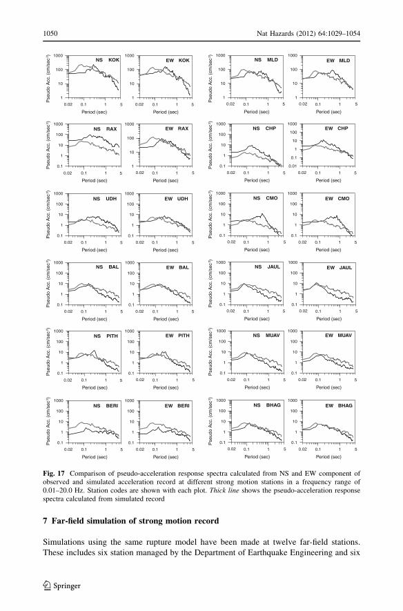
Fig. 17 Comparison of pseudo-acceleration response spectra calculated from NS and EW component ofobserved and simulated acceleration record at different strong motion stations in a frequency range of0.01–20.0 Hz. Station codes are shown with each plot. Thick line shows the pseudo-acceleration responsespectra calculated from simulated record

1050 Nat Hazards (2012) 64:1029–1054

123

in the Kumaon network managed by the Department of Earth Sciences. Stations of Ku-

maon network are placed at an epicentral distance ranging between 886 and 944 km.

Information of these far-field stations is given in Table 7 at which ground motion record

has been simulated by using the technique given in the present paper. The simulated NS

and EW component of acceleration record has been compared with the observed accel-

eration record in the same frequency range as used for its processing and is shown in

Fig. 16. A pseudo-acceleration response spectrum has been computed for simulated and

observed record and their comparison is shown in Fig. 17.

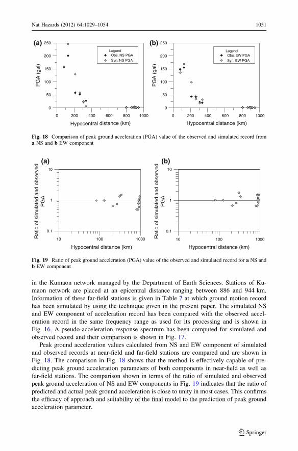
Peak ground acceleration values calculated from NS and EW component of simulated

and observed records at near-field and far-field stations are compared and are shown in

Fig. 18. The comparison in Fig. 18 shows that the method is effectively capable of pre-

dicting peak ground acceleration parameters of both components in near-field as well as

far-field stations. The comparison shown in terms of the ratio of simulated and observed

peak ground acceleration of NS and EW components in Fig. 19 indicates that the ratio of

predicted and actual peak ground acceleration is close to unity in most cases. This confirms

the efficacy of approach and suitability of the final model to the prediction of peak ground

acceleration parameter.

Hypocentral distance (km)

0

50

100

150

200

250P

GA

(ga

l)

LegendObs. NS PGASyn. NS PGA

Hypocentral distance (km)

0

50

100

150

200

250

PG

A (

gal)

LegendObs. EW PGASyn. EW PGA

(a) (b)

0 200 400 600 800 1000 0 200 400 600 800 1000

Fig. 18 Comparison of peak ground acceleration (PGA) value of the observed and simulated record froma NS and b EW component

Hypocentral distance (km)

0.1

1

10

Rat

io o

f sim

ulat

ed a

nd o

bser

ved

PG

A

10 100 100010 100 1000

Hypocentral distance (km)

0.1

1

10

Rat

io o

f sim

ulat

ed a

nd o

bser

ved

PG

A(a) (b)

Fig. 19 Ratio of peak ground acceleration (PGA) value of the observed and simulated record for a NS andb EW component

Nat Hazards (2012) 64:1029–1054 1051

123

The simulations made from present technique at near-field and far-field stations are

quantitatively compared with observed records. The quantitative comparison of simulated

and observed record has been made in terms of root mean square error given in Eq. (17).

The calculated root mean square error between observed and simulated records and its

response spectra are given in Table 8. It is seen that root mean square error between

observed and simulated accelerogram varies from 0.46 to 0.56 at the near-field stations and

from 0.32 to 0.62 at the far-field stations, respectively. The root mean square error between

response spectrums of observed and simulated records varies from 0.65 to 2.58 at the near-

field stations and from 0.34 to 2.28 at the far-field stations, respectively. The quantitative

comparison indicates that the range of uncertainty in simulated and observed acceleration

record at far-field stations are higher as compared to the near-field stations. This may be

resulted from several factors which are actually present in the ray path between source and

far-field recording stations which are not included in the present approach of simulation.

These effects include large-scale crustal deformation and heterogeneities present in the

path between source and receiver for far-field stations.

8 Conclusions

This paper presents modified semi-empirical approach given by Midorikawa (1993) for

component wise simulation of strong ground motion. Modifications in the semi-empirical

approach are made to remove dependency of this method purely on attenuation relation. In

the present work, seismic moment is used in place of attenuation relation to scale the

envelope function used in semi-empirical approach. The method has been tested for

simulation of near-field and far-field acceleration record of the Sikkim earthquake

(Mw = 6.9) of September 18, 2011. Several possibilities of modeling parameters like

Table 8 Estimated RMSEbetween observed and simulatedacceleration record and itsresponse spectrum

Stations RMSE between observed andsimulated acceleration timeseries

RMSE between observedand simulated responsespectrum

NS EW NS EW

GTK 0.48 0.46 0.87 0.65

SLG 0.46 0.56 2.58 1.19

COB 0.53 0.52 1.84 2.28

KOK 0.57 0.58 1.18 1.55

MLD 0.47 0.47 1.03 0.34

RAX 0.62 0.43 0.78 0.81

CHP 0.46 0.45 0.49 0.65

UDH 0.35 0.32 0.54 0.38

CMO 0.54 0.55 1.03 0.74

BAL 0.42 0.43 2.08 1.96

JAUL 0.46 0.48 2.00 2.28

PITH 0.37 0.37 1.84 1.40

MUAV 0.39 0.40 2.20 1.51

BERI 0.54 0.55 1.30 1.40

BHAG 0.50 0.53 1.27 1.08

1052 Nat Hazards (2012) 64:1029–1054

123

position of nucleation point, rupture velocity, and the dip of the rupture plane have been

considered before arising to a final model. The selection of final model is based on root

mean square error of simulated and observed waveform. Comparison of several rupture

models in terms of root mean square error shows that minimum error is associated with

southward propagating rupture of the Sikkim earthquake. Records have been simulated for

various near-field and far-field stations using the final rupture model of the Sikkim

earthquake. Component wise comparison of simulated and observed accelerogram at

various stations confirms the efficacy of the approach for modeling of near-field and far-

field ground motion.

Acknowledgments The authors sincerely thank Ministry of Earth Sciences (MoES), Government of Indiasupported project (Grant no: MoES/P.O.(Seismo)/1(42)/2009) for providing far-field strong motion data.The near-field data obtained from http://www.pesmos.in are thankfully acknowledged.

References

Boore DM (1983) Stochastic simulation of high frequency ground motion based on seismological models ofradiated Spectra. Bull Seism Soc Am 73:1865–1894

Boore DM, Joyner WB (1991) Estimation of ground motion at deep soil sites in eastern North America. BullSeims Soc Am 81:2167–2185

Brocher TM (2005) Empirical relations between elastic wave speeds and density in the Earth’s crust. BullSeism Soc Am 95:2081–2092

Brune JN (1970) Tectonic stress and spectra of seismic shear waves from earthquakes. J Geophys Res75:4997–5009

Cotte N, Pedersen H, Campillo M, Mars J, Ni J, Kind R, Sandvol E, Zhao W (1999) Determination of thecrustal structure in Southern Tibet by dispersion and amplitude analysis of Rayleigh waves. Geophys JInt 138:809–819

Dasgupta S, Ganguly J, Neogi S (2004) Inverted metamorphic sequence in the Sikkim Himalayas: crys-talline history, P-T gradient and implications. J Metamorp Geol 22:395–412

Fukuyama E, Irikura K (1986) Rupture process of the 1983 Japan sea (Akita-Oki) earthquake using awaveform inversion method. Bull Seism Soc Am 76:1623–1640

Hadley DM, Helmberger DV (1980) Simulation of ground motions. Bull Seism Soc Am 70:610–617Hadley DM, Helmberger DV, Orcutt JA (1982) Peak acceleration scaling studies. Bull Seism Soc Am

72:959–979Hanks TC, McGuire RK (1981) The character of high frequency ground motion. Bull Seism Soc Am

71:2071–2095Hartzell SH (1978) Earthquake aftershocks as Green’s functions. Geophys Res Lett 5:1–4Hartzell SH (1982) Simulation of ground accelerations for May 1980 Mammoth Lakes, California earth-

quakes. Bull Seism Soc Am 72:2381–2387Hazarika P, Kumar MR, Srijayanthi G, Raju PS, Rao NP, Srinagesh D (2010) Transverse tectonics in the

Sikkim Himalaya: evidence from seismicity and focal-mechanism data. Bull Seism Soc Am100(4):1816–1822. doi:10.1785/0120090339

Heaton TH, Hartzell SH (1989) Estimation of strong ground motions from hypothetical earthquakes on theCascadia subduction zone, Pacific Northwest. Pure Appl Geophys 129:131–201

Housner GW, Jennings PC (1964) Generation of artificial earthquakes. Proc ASCE 90:113–150Houston H, Kanamori H (1984) The effect of asperities on short period seismic radiation with application on

rupture process and strong motion. Bull Seism Soc Am 76:19–42Hutchings L (1985) Modeling earthquakes with empirical Green’s functions (abs). Earthq Notes 56:14Imagawa K, Mikami N, Mikumo T (1984) Analytical and semi empirical synthesis of near field seismic

waveforms for investigating the rupture mechanism of major earthquakes. J Phys Earth 32:317–338Irikura K (1983) Semi empirical estimation of strong ground motion during large earthquakes. Bull Dis

Prevent Res Inst 33:63–104Irikura K, Kamae K (1994) Estimation of strong ground motion in broad-frequency band based on a seismic

source scaling model and an Empirical Green’s function technique. Ann Geofis XXXVII 6:1721–1743Irikura K, Muramatu I (1982) Synthesis of strong ground motions from large earthquakes using observed

seismograms of small events. In: Proceedings of the third international Microzonation conference,Seattle, pp. 447–458

Nat Hazards (2012) 64:1029–1054 1053

123

Irikura K, Kagawa T, Sekiguchi H (1997) Revision of the empirical Green’s function method by Irikura,1986. Programme and abstracts. Seismol Soc Jpn 2:B25

Joshi A (2004) A simplified technique for simulating wide band strong ground motion for two recentHimalaya earthquakes. Pure Appl Geophys 161:1777–1805

Joshi A, Midorikawa S (2004) A simplified method for simulation of strong ground motion using rupturemodel of the earthquake source. J Seism 8:467–484

Joshi A, Mohan K (2008) Simulation of accelerograms from simplified deterministic approach for the 23rdOctober 2004 Niigata-ken Chuetsu earthquake. J Seismol 12:35–51

Joshi A, Singh S, Giroti K (2001) The simulation of ground motions using envelope summations. Pure ApplGeophys 158:877–901

Joshi A, Mohanty M, Bansal AR, Dimri VP, Chadha RK (2010) Use of spectral acceleration data fordetermination of three-dimensional attenuation structure in the Pithoragarh region of KumaonHimalaya. J Seism 14:247–272

Joshi A, Pushpa K, Sharma ML, Ghosh AK, Agarwal MK, Ravikiran A (2012) A strong motion model of the2004 great Sumatra earthquake: simulation using a modified semi empirical method. J Earthq Tsunami(in press)

Joyner WB, Boore DM (1988) Measurement, characterization and prediction of strong ground motion. In:Proceedings of earthquake engineering and soil dynamics II, Utah, June 27–30, pp 43–100

Kameda H, Sugito M (1978) Prediction of strong earthquake motions by evolutionary process model. In:Proceedings of the sixth Japan earthquake engineering symposium, pp 41–48

Kanamori H (1979) A semi empirical approach to prediction of long period ground motions from greatearthquakes. Bull Seism Soc Am 69:1645–1670

Kanamori H, Anderson DL (1975) Theoretical basis of some empirical relations in seismology. Bull SeismSoc Am 65:1073–1095

Kayal JR (2001) Microearthquake activity in some parts of the Himalaya and tectonic model. Tectono-physics 339:331–351

Khattri KN, Zeng Y, Anderson JG, Brune J (1994) Inversion of strong motion waveforms for source slipfunction of 1991 Uttarkashi earthquake, Himalaya. J Himalayan Geol 5:163–191

Lai SP (1982) Statistical characterization of strong ground motions using power spectral density function.Bull Seism Soc Am 72:259–274

Lay T, Wallace TC (1995) Modern global seismology. Academic Press, California 521 ppMcGuire RK, Becker AM, Donovan NC (1984) Spectral estimates of seismic shear waves. Bull Seism Soc

Am 74:2167–2185Midorikawa S (1989) Synthesis of ground acceleration of large earthquakes using acceleration envelope

waveform of small earthquake. J Struct Construct Eng 398:23–30Midorikawa S (1993) Semi empirical estimation of peak ground acceleration from large earthquakes.

Tectonophysics 218:287–295Mikumo T, Irikura K, Imagawa K (1981) Near field strong motion synthesis from foreshock and aftershock

records and rupture process of the main shock fault (abs.). IASPEI 21st General Assembly, LondonMunguia L, Brune JM (1984) Simulations of strong ground motions for earthquakes in the Mexicali-

Imperial Valley. In: Proceedings of workshop on strong ground motion simulation and earthquakeengineering applications, Pub. 85-02. Earthquake Engineering Research Institute, Los Altos, California21-1-21-19

Nath SK, Thingbaijam KKS (2009) Seismic hazard assessment—a holistic microzonation approach. NatHazards Earth Syst Sci 9:1445–1459

Nath SK, Vyas M, Pal I, Sengupta P (2005) A Seismic hazard scenario in the Sikkim Himalaya fromseismotectonics, spectral amplification, source parameterization and spectral attenuation laws usingstrong motion seismometry. J Geophy Res 110:B01301. doi:10.1029/2004JB003199

Sinozuka M, Sato Y (1967) Simulation of nonstationary random process. Proc ASCE 93:11–40Tapponnier P, Molnar P (1977) Active faulting and tectonics in China. J Geophy Res 82:2905–2930Wells LD, Coppersmith KJ (1994) New empirical relationships among magnitude, rupture length, rupture

width, rupture area and surface displacement. Bull Seism Soc Am 84:974–1002Yu G (1994) Some aspects of earthquake seismology: slip portioning along major convergent plate

boundaries: composite source model for estimation of strong motion and non linear soil responsemodeling. Ph.D. thesis, University of Nevada

Yu G, Khattri KN, Anderson JG, Brune JN, Zeng Y (1995) Strong ground motion from the Uttarkashi,Himalaya, India, earthquake: comparison of observations with synthetics using the composite sourcemodel. Bull Seism Soc Am 85:31–50

Zeng Y, Anderson JG, Su F (1994) A composite source model for computing realistic synthetic strongground motions. Geophys Res Lett 21:725–728

1054 Nat Hazards (2012) 64:1029–1054

123