REPORT NO. EERC 2007-03 EARTHQUAKE ENGINEERING RESEARCH CENTER NEAR-FAUlT SEISMIC GROUND MOTIONS DOUGLAS DREGER GABRIEL HURTADO ANIL K. CHOPRA SHAWN LARSEN COLLEGE OF ENGINEERING UNIVERSITY OF CALIFORNIA, BERKELEY

Welcome message from author
This document is posted to help you gain knowledge. Please leave a comment to let me know what you think about it! Share it to your friends and learn new things together.
Transcript
REPORT NO. EERC 2007-03 EARTHQUAKE ENGINEERING RESEARCH CENTER
NEAR-FAUlT SEISMIC GROUND MOTIONS
DOUGLAS DREGER GABRIEL HURTADO ANIL K. CHOPRA SHAWN LARSEN
COLLEGE OF ENGINEERING UNIVERSITY OF CALIFORNIA, BERKELEY

This page is left blank
Near-Fault Seismic Ground Motions
By Douglas Dreger Gabriel Hurtado
Anil Chopra University of California, Berkeley
and Shawn Larsen
Lawrence Livermore National Laboratory
Research conducted for the California Department of Transportation
Under contract 59A0435
Earthquake Engineering Research Center
University of California, Berkeley
October, 2007
UCB/EERC 2007-03

This page is left blank
Near-Fault Seismic Ground Motions
Douglas Dreger1, Gabriel Hurtado1, Anil Chopra1, and Shawn Larsen2
1. University of California Berkeley 2. Lawrence Livermore National Laboratory
Abstract
Bridges that cross faults are subject to static deformation that occurs close in time to the arrival of dynamic pulse-like ground motions. Static offsets can be as large as several centimeters to 10s of meters and strong ground motion velocity pulses exceeding 100 cm/s have been observed. Near-fault records, in the distance range of 10 to 100s of meters from faults are essentially nonexistent except for a few cases, and therefore numerical simulation of ground motions for such near-fault situations is necessary. We simulate ground motions to 17.5 Hz, 15-100m from the fault for a Mw6.5 earthquake using an elastic finite-difference code. Simulations for homogeneous Earth structure are compared for uniform and heterogeneous fault rupture scenarios. To investigate asymmetry of ground motions on opposite sides of a dipping reverse fault we used the dislocation method of Okada (1992) to compute static offset. From those results we develop a simplified procedure for the simulation of near-fault time histories. All of the simulations assume linear elasticity, and it is noted that the computed strain is as high as 10-4 - 10-3, and it is likely that there would be significant non-linear behavior in this near-fault region.
Introduction
Bridges that cross faults can be subjected to large dynamic and static ground motions. As there are very few actual ground motions recorded very close to ruptured faults (< 100m) ground motion simulation is the only viable way to obtain time histories for structural analysis. The research project seeks to develop simplified procedures for the characterization of the response of bridges that cross faults, accounting for both dynamic and static ground motions, and this paper presents the seismic ground motion simulation results.
Bridges with a minimum span of 30m are considered, and ground motion simulations were carried out with a closest distance to the fault of 15m. The simulated time histories must accurately incorporate the near-fault source radiation pattern, account for far- and near-field seismic radiation, and have the ability to characterize motions for a broad range of fault types (e.g. vertical strike-slip and reverse faulting), as well as variable slip and full kinematic description of the rupture process. We must be able to accurately simulate the directivity effect as well as the sudden elastic rebound sometimes referred to as fling. The 3D elastic finite-difference code e3d (Larsen and Schultz, 1995) satisfies these requirements and has undergone validation testing as part of the PEER/SCEC project to verify numerical algorithms for ground motion simulation. Because of the need to compute motions very close to the fault and at high frequency this poses a significant computational challenge.
Simulation Method
The simulation method that we use is a 4th order accurate staggered-grid elastic finite-difference code, e3d, developed at Lawrence Livermore National Laboratory (LLNL) (Larsen and Schultz, 1995). Stress-free boundary conditions are used to model the free-surface, and absorbing boundary conditions (Clayton and Engquist, 1977) are used to damp artificial reflections from the grid boundary. This code was tested and calibrated in a PEER/SCEC funded effort to verify
numerical methods for ground motion simulation. We have used this code in numerous studies of three-dimensional ground motion modeling (Stidham et al., 1999; Panning et al., 2000; Dolenc et al., 2005) as well as in ongoing work studying the Santa Clara Valley and the Napa Valley.
The advantage of using a finite-difference code is that it is capable of simulating complete seismic waveforms in three-directions of motion that are complete in terms of near-, intermediate-, and far-field terms of the solution to the elasto-dynamic equation of motion. We use a high spatial resolution (fine grid discretization) to obtain the motions close to the fault. The high spatial resolution also improves the representation of the kinematic rupture process by allowing smooth evolution of the propagating rupture front and slip rise time on the fault. The obvious benefit of this approach is that the source representation is the same as in the ground motion computation. Finally, the method also allows the straightforward incorporation of rupture heterogeneity and seismic velocity structure including 3D velocity structure if warranted.
2
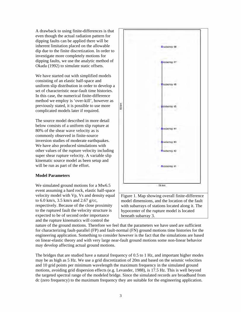
Figure 1. Map showing overall finite-difference model dimensions, and the location of the fault with subarrays of stations located along it. The hypocenter of the rupture model is located beneath subarray 3.
A drawback to using finite-differences is that even though the actual radiation pattern for dipping faults can be applied there will be inherent limitation placed on the allowable dip due to the finite discretization. In order to investigate more completely motions for dipping faults, we use the analytic method of Okada (1992) to simulate static offsets.
We have started out with simplified models consisting of an elastic half-space and uniform slip distribution in order to develop a set of characteristic near-fault time histories. In this case, the numerical finite-difference method we employ is ‘over-kill’, however as previously stated, it is possible to use more complicated models later if required.
The source model described in more detail below consists of a uniform slip rupture at 80% of the shear wave velocity as is commonly observed in finite-source inversion studies of moderate earthquakes. We have also produced simulations with other values of the rupture velocity including super shear rupture velocity. A variable slip kinematic source model as been setup and will be run as part of the effort.
Model Parameters
We simulated ground motions for a Mw6.5 event assuming a hard rock, elastic half-space velocity model with Vp, Vs and density equal to 6.0 km/s, 3.5 km/s and 2.67 g/cc, respectively. Because of the close proximity to the ruptured fault the velocity structure is expected to be of second order importance and the rupture kinematics will control the nature of the ground motions. Therefore we feel that the parameters we have used are sufficient for characterizing fault-parallel (FP) and fault-normal (FN) ground motions time histories for the engineering application. Something to consider however is the fact that the simulations are based on linear-elastic theory and with very large near-fault ground motions some non-linear behavior may develop affecting actual ground motions.
The bridges that are studied have a natural frequency of 0.5 to 1 Hz, and important higher modes may be as high as 5 Hz. We use a grid discretization of 20m and based on the seismic velocities and 10 grid points per minimum wavelength the maximum frequency in the simulated ground motions, avoiding grid dispersion effects (e.g. Levander, 1988), is 17.5 Hz. This is well beyond the targeted spectral range of the modeled bridge. Since the simulated records are broadband from dc (zero frequency) to the maximum frequency they are suitable for the engineering application.
3
The parameters we have used were chosen to allow for future simulations incorporating lower seismic velocity while maintaining the required bandwidth.
From the magnitude the fault length and width were determined to be 28.8 km, and 9.3 km respectively, based on the relations from Wells and Coppersmith (1994).
With this fault area and the scalar seismic moment obtained from the moment magnitude relationship the average slip on the fault is 0.71m.
0.71m is a large amount of differential offset for a bridge to accommodate. If a realistic non-uniform slip distribution were used there would be points along the fault with offsets both smaller and larger than the average value we use. This is demonstrated with a series of three heterogeneous slip simulations.
The finite difference model space is 50x25x15 km3 and as Figure 1 shows the fault is centered in the model. The model dimensions are large to ensure that grid finiteness does not affect the simulation results by introducing reflection artifacts or errors in computing the static offset. The finite-difference grid has a spacing of 20m resulting in 2.3 billion grid points and a total required computer memory of 121.8 Gbytes. The simulations were run on a distributed memory super computer at the Lawrence Livermore National Laboratory.
Arrays of stations are located along the fault as shown in Figure 1. The subarrays each contain recording stations set at regular distance from the fault (Figure 2). Subarrays 1 and 8 are off the ends of the fault, 2 and 7 are at the ends of the fault. The rest of the subarrays are located along the fault with the closest station being only 15m from it. The hypocenter is located beneath subarray 3. Thus the rupture proceeds from south to north in Figure 1, from subarray 3 to 7. Directivity focusing is therefore expected to be strong on the FN component for the strike-slip case at subarrays 4-8. FP motions should be strong at subarrays 2-7. Subarrays 1 and 8, because they are each located 5 km from the fault, are expected to have insignificant FP motions in the strike-slip case. The simulated ground motions are discussed in detail in the next section.
4
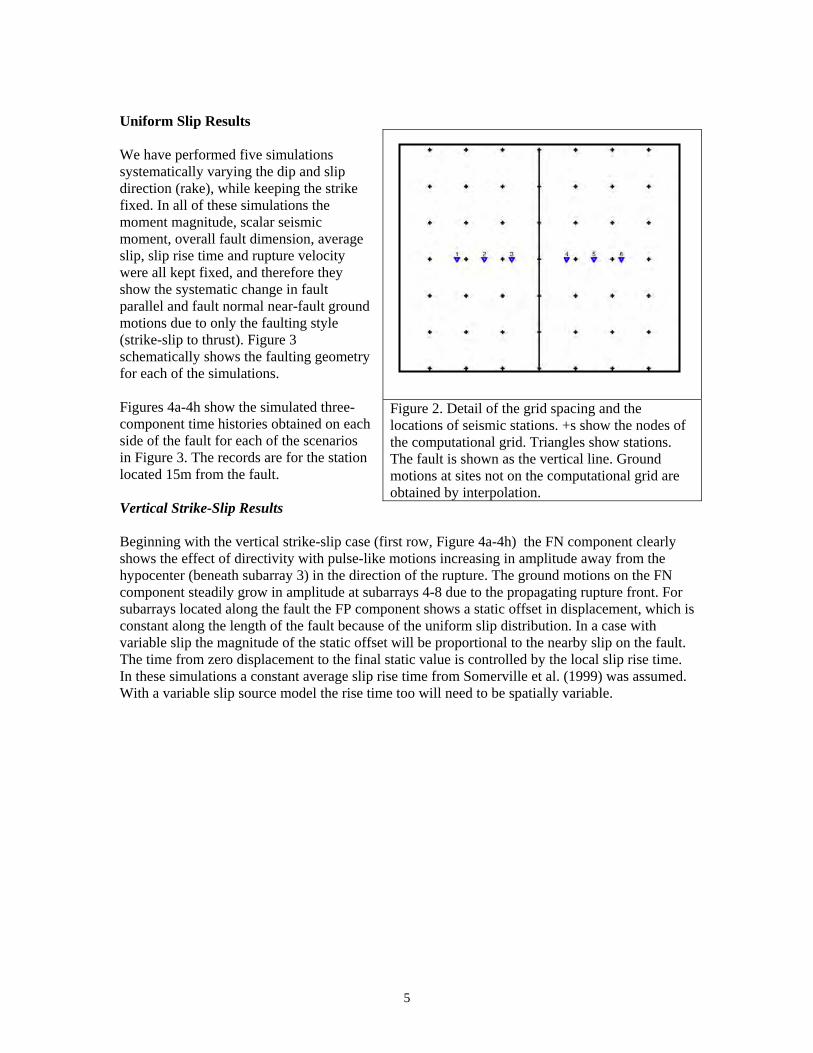
Figure 2. Detail of the grid spacing and the locations of seismic stations. +s show the nodes of the computational grid. Triangles show stations. The fault is shown as the vertical line. Ground motions at sites not on the computational grid are obtained by interpolation.
Uniform Slip Results
We have performed five simulations systematically varying the dip and slip direction (rake), while keeping the strike fixed. In all of these simulations the moment magnitude, scalar seismic moment, overall fault dimension, average slip, slip rise time and rupture velocity were all kept fixed, and therefore they show the systematic change in fault parallel and fault normal near-fault ground motions due to only the faulting style (strike-slip to thrust). Figure 3 schematically shows the faulting geometry for each of the simulations.
Figures 4a-4h show the simulated three-component time histories obtained on each side of the fault for each of the scenarios in Figure 3. The records are for the station located 15m from the fault.
Vertical Strike-Slip Results
Beginning with the vertical strike-slip case (first row, Figure 4a-4h) the FN component clearly shows the effect of directivity with pulse-like motions increasing in amplitude away from the hypocenter (beneath subarray 3) in the direction of the rupture. The ground motions on the FN component steadily grow in amplitude at subarrays 4-8 due to the propagating rupture front. For subarrays located along the fault the FP component shows a static offset in displacement, which is constant along the length of the fault because of the uniform slip distribution. In a case with variable slip the magnitude of the static offset will be proportional to the nearby slip on the fault. The time from zero displacement to the final static value is controlled by the local slip rise time. In these simulations a constant average slip rise time from Somerville et al. (1999) was assumed. With a variable slip source model the rise time too will need to be spatially variable.
5
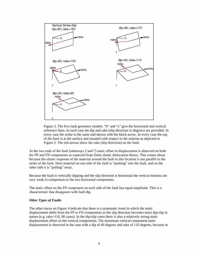
Figure 3. The five fault geometry models. “h” and “z” give the horizontal and vertical reference lines. In each case the dip and rake (slip direction in degrees) are provided. In every case the strike is the same and shown with the black arrow. In every case the top of the fault is at the surface and situated with respect to the stations as depicted in Figure 2. The red arrows show the rake (slip direction) on the fault.
At the two ends of the fault (subarrays 2 and 7) static offset in displacement is observed on both the FP and FN components as expected from finite elastic dislocation theory. This comes about because the elastic response of the material around the fault in this location is not parallel to the strike of the fault. Here material on one side of the fault is “pushing” into the fault, and on the other side it is “pulling” away.
Because the fault is vertically dipping and the slip direction is horizontal the vertical motions are very weak in comparison to the two horizontal components.
The static offset on the FP component on each side of the fault has equal amplitude. This is a characteristic that disappears with fault dip.
Other Types of Faults
The other traces on Figure 4 indicate that there is a systematic trend in which the static displacement shifts from the FP to FN components as the slip direction becomes more dip-slip in nature (e.g. rake=110, 90 cases). In the dip-slip cases there is also a relatively strong static displacement offset on the vertical components. The maximum vertical component static displacement is observed in the case with a dip of 40 degrees and rake of 110 degrees, because in
6
the thrust case (dip=20 degrees and rake=90 degrees) the shallow dip produces a slip vector that is nearly horizontal.
Similar behavior in the simulated ground motions would be observed in models transitioning from strike-slip to normal faulting.
The static offset on the FN component for dip-slip cases is asymmetrical in amplitude on the two sides of the fault. The hanging block has systematically higher amplitude motions, which is due to the fact that stations on that side of the fault are systematically closer to all points on the fault, and because of the unbounded nature of the free-surface. In a later section using analytic dislocation theory we develop a method for determining the partitioning of slip on opposite sides of the fault for reverse dip-slip cases.
General Observations
The uniform slip simulations show that waveforms at adjacent sites for a given fault geometry are very similar. Amplitudes may vary due to differing degrees of directivity but the waveforms remain similar. This is likely to remain true even in cases with heterogeneous velocity structure since the dominant contribution to the waveforms at this close distance come from the directivity and nearby fault offset. Since the component with a strong fling contribution remains constant over the length of the fault the changes in amplitude of the directivity-dominant component lead to significant differences in the total vector ground motion along the length of the fault.
A variable slip distribution will affect both the directivity component and also the static offsets, which will be proportional to the local fault slip. However, even in this case we expect the general shape of the near-fault time histories to remain pulse-like and quite similar to what is presented in this paper. This is shown to be the case in a later section of the report.
Seismic velocity model complexity in the form of velocity contrast across the fault, or a fault zone with a low velocity gouge are expected to be important in site-specific ground motions at sites located close to the fault or within the low velocity fault zone. These are model complications that were beyond the scope of the proposed study, but we have performed a simulation that shows that FP motions are unaffected for near-fault sites, and that there can be a substantial effect on the FN motions for the vertical strike-slip case.
Another general observation is that motions at the ends of the fault are more complex than along the fault or off of the ends of the fault and for the vertical strike-slip case static offsets are observed on both the FP and FN components. This comes about simply from the elastic response of material around the fault in which material “pushes” into the fault from two opposite quadrants, and “pulls” away from the other two opposite quadrants. Although not as pronounced in the simulations for the other fault styles the time histories at sites located on the ends of the fault display greater complexity than sites along the length of the fault or off of the ends of the fault.
In general the simulations show that both static offsets and dynamic directivity controlled pulses need to be considered on any of the three components to account for possible faulting variability.
For the predominantly strike-slip simulations (rake 150-180 degrees) the static offset on the FP component is symmetric across the fault with respect to amplitude (rows 1 and 2, Figures 4b-4g). This does not hold for the predominantly dip-slip cases (rows 4 and 5, Figures 4b-4g). In these cases it is found that the static offsets are anti-symmetric with respect to amplitude. The foot-
7
block (the side where the fault is dipping away from) clearly has much lower static offset than the hanging block. In the figures the hanging block is on the right side of the fault trace. Even though the stations on either side of the fault are the same distance to the surface trace, the station on the hanging block is closer to a greater surface area of the fault resulting in the larger ground motions on that side. This is also true for the velocity pulses. Elevated ground motions have been observed on the hanging block side of the fault in the Chi-Chi, Taiwan Mw7.6 thrust earthquake (e.g. Chi et al., 2001). Empirical ground motion attenuation relationships have also accounted for larger observed motions on the hanging block of reverse events (e.g. Abrahamson and Silva, 1997).
Velocity Response
Large amplitude pulse-like velocity ground motions can occur on all three components depending on the faulting style. The difference between directivity and fault slip control of the velocity pulses on the FN and FP components is illustrated in Figures 5 and 6. In Figure 5, the top row shows the three-component records at subarray 3 for the vertical strike-slip case. The other rows show the velocity records for subarrays 4-8. On the FN component it is clear that the velocity pulse grows with distance along the fault as the rupture directivity amplifies the motion. In contrast, at subarrays 3-6 the FP velocity pulse is constant amplitude and represents the slip velocity locally on the fault. At subarray 7, at the end of the fault, the FP amplitude decreases because the elastic response is not parallel to the fault. The sign of the FN static component is opposite and therefore the ground motions on the FN component are reduced by destructive interference of the directivity and the fault fling pulses. At subarray 8 only the FN component has significant amplitude, as this site is located off of the edge of the fault. This result shows that even for a uniform slip case, because of the different effects of directivity and fling, there can be significant variation in the relative amplitudes of FN and FP velocity pulses and therefore the total vector ground motion.
In Figure 6 velocity records at the same stations are compared for the 40-degree dipping reverse-slip case. Here directivity is evident on the FP component though it is much less pronounced. The FN component is controlled by the fault fling. At subarrays 3 and 4 the slightly higher amplitudes and elevated high frequency content result from a slight updip directivity effect.
Maximum directivity occurs when the slip direction and the rupture direction are the same (Aagaard et al., 2004). In the case of a long dip-slip rupture, such as occurred in the 1999 Mw7.6 Chi Chi, Taiwan (Chi et al., 2001) and the Mw6.5 San Simeon (Dreger et al., 2005), California earthquakes directivity is observed, however since the slip directions in these events were perpendicular to the rupture direction it was a minimum directivity effect. Comparison of the velocity records in Figures 5 and 6 demonstrate the reduced lateral directivity in the dip-slip style of faulting compared to the strike-slip type.
8
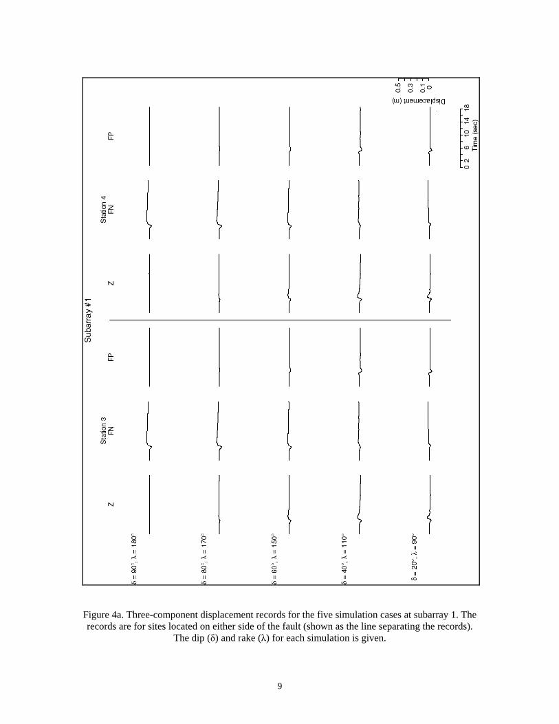
Figure 4a. Three-component displacement records for the five simulation cases at subarray 1. The records are for sites located on either side of the fault (shown as the line separating the records).
The dip (δ) and rake (λ) for each simulation is given.
9
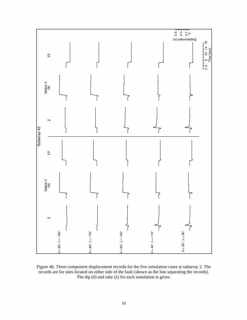
Figure 4b. Three-component displacement records for the five simulation cases at subarray 2. The records are for sites located on either side of the fault (shown as the line separating the records).
The dip (δ) and rake (λ) for each simulation is given.
10
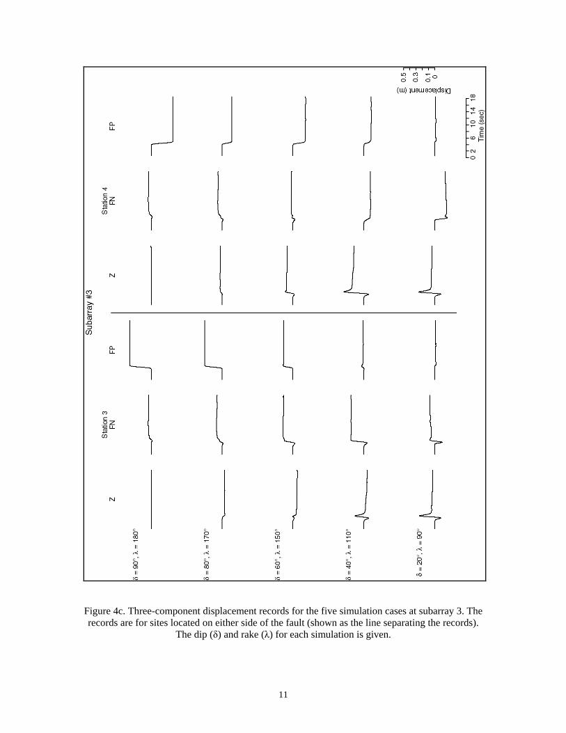
Figure 4c. Three-component displacement records for the five simulation cases at subarray 3. The records are for sites located on either side of the fault (shown as the line separating the records).
The dip (δ) and rake (λ) for each simulation is given.
11

Figure 4d. Three-component displacement records for the five simulation cases at subarray 4. The records are for sites located on either side of the fault (shown as the line separating the
records). The dip (δ) and rake (λ) for each simulation is given.
12
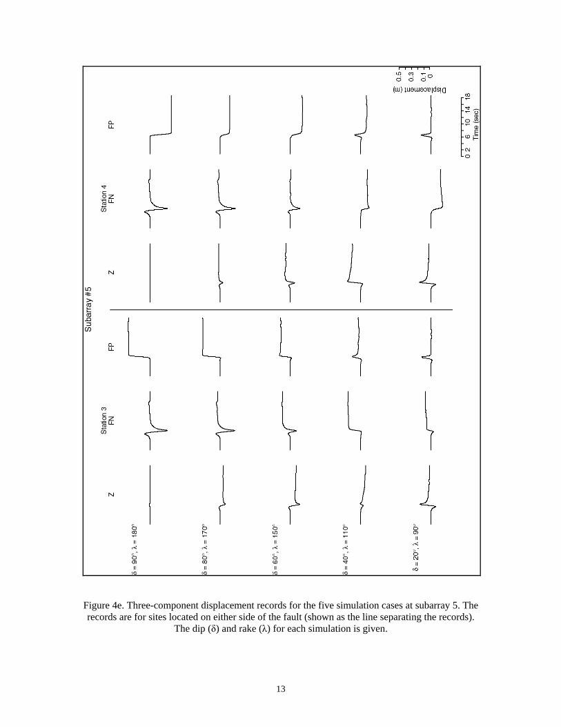
Figure 4e. Three-component displacement records for the five simulation cases at subarray 5. The records are for sites located on either side of the fault (shown as the line separating the records).
The dip (δ) and rake (λ) for each simulation is given.
13
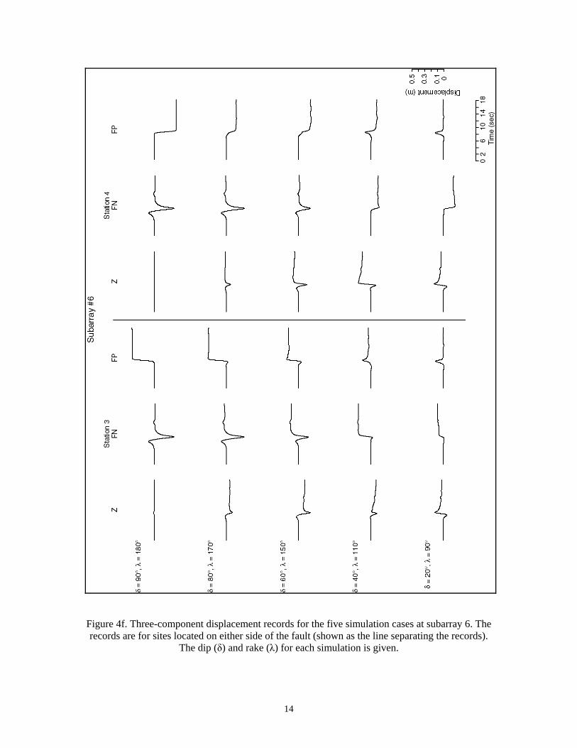
Figure 4f. Three-component displacement records for the five simulation cases at subarray 6. The records are for sites located on either side of the fault (shown as the line separating the records).
The dip (δ) and rake (λ) for each simulation is given.
14
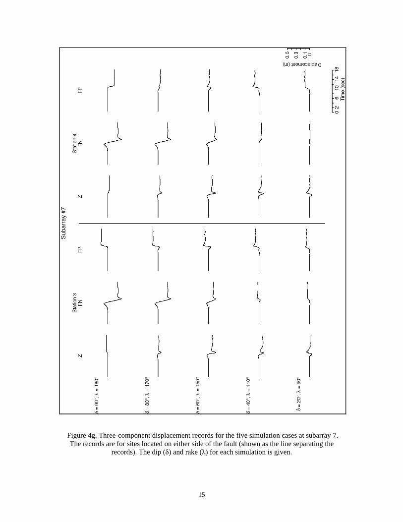
Figure 4g. Three-component displacement records for the five simulation cases at subarray 7. The records are for sites located on either side of the fault (shown as the line separating the
records). The dip (δ) and rake (λ) for each simulation is given.
15
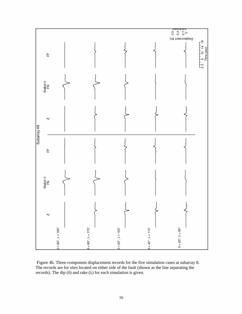
Figure 4h. Three-component displacement records for the five simulation cases at subarray 8. The records are for sites located on either side of the fault (shown as the line separating the records). The dip (δ) and rake (λ) for each simulation is given.
16
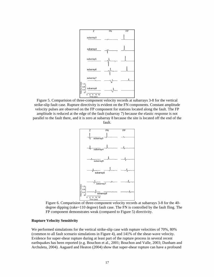
Figure 5. Comparision of three-component velocity records at subarrays 3-8 for the vertical strike-slip fault case. Rupture directivity is evident on the FN components. Constant amplitude velocity pulses are observed on the FP component for stations located along the fault. The FP amplitude is reduced at the edge of the fault (subarray 7) because the elastic response is not
parallel to the fault there, and it is zero at subarray 8 because the site is located off the end of the fault.
Figure 6. Comparision of three-component velocity records at subarrays 3-8 for the 40-degree dipping (rake=110 degree) fault case. The FN is controlled by the fault fling. The FP component demonstrates weak (compared to Figure 5) directivity.
Rupture Velocity Sensitivity
We performed simulations for the vertical strike-slip case with rupture velocities of 70%, 80% (common to all fault scenario simulations in Figure 4), and 141% of the shear-wave velocity. Evidence for super-shear rupture during at least part of the rupture process in several recent earthquakes has been reported (e.g. Bouchon et al., 2001; Bouchon and Valle, 2003; Dunham and Archuleta, 2004). Aagaard and Heaton (2004) show that super-shear rupture can have a profound
17
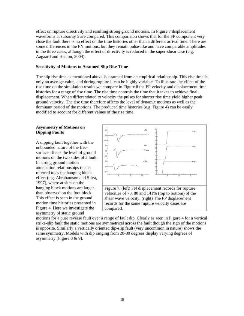
effect on rupture directivity and resulting strong ground motions. In Figure 7 displacement waveforms at subarray 5 are compared. This comparision shows that for the FP component very close the fault there is no effect on the time histories other than a different arrival time. There are some differences in the FN motions, but they remain pulse-like and have comparable amplitudes in the three cases, although the effect of directivity is reduced in the super-shear case (e.g. Aagaard and Heaton, 2004).
Sensitivity of Motions to Assumed Slip Rise Time
The slip rise time as mentioned above is assumed from an empirical relationship. This rise time is only an average value, and during rupture it can be highly variable. To illustrate the effect of the rise time on the simulation results we compare in Figure 8 the FP velocity and displacement time histories for a range of rise time. The rise time controls the time that it takes to achieve final displacement. When differentiated to velocity the pulses for shorter rise time yield higher peak ground velocity. The rise time therefore affects the level of dynamic motions as well as the dominant period of the motions. The produced time histories (e.g. Figure 4) can be easily modified to account for different values of the rise time.
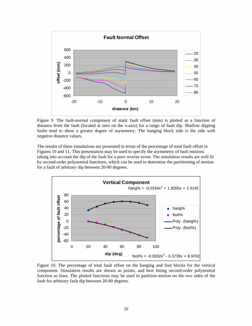
Asymmetry of Motions on Dipping Faults
A dipping fault together with the unbounded nature of the free-surface affects the level of ground motions on the two sides of a fault. In strong ground motion attenuation relationships this is referred to as the hanging block effect (e.g. Abrahamson and Silva, 1997), where at sites on the hanging block motions are larger than observed on the foot block. This effect is seen in the ground motion time histories presented in Figure 4. Here we investigate the asymmetry of static ground motions for a pure reverse fault over a range of fault dip. Clearly as seen in Figure 4 for a vertical strike-slip fault the static motions are symmetrical across the fault though the sign of the motions is opposite. Similarly a vertically oriented dip-slip fault (very uncommon in nature) shows the same symmetry. Models with dip ranging from 20-80 degrees display varying degrees of asymmetry (Figure 8 & 9).
Figure 7. (left) FN displacement records for rupture velocities of 70, 80 and 141% (top to bottom) of the shear wave velocity. (right) The FP displacement records for the same rupture velocity cases are compared.
18
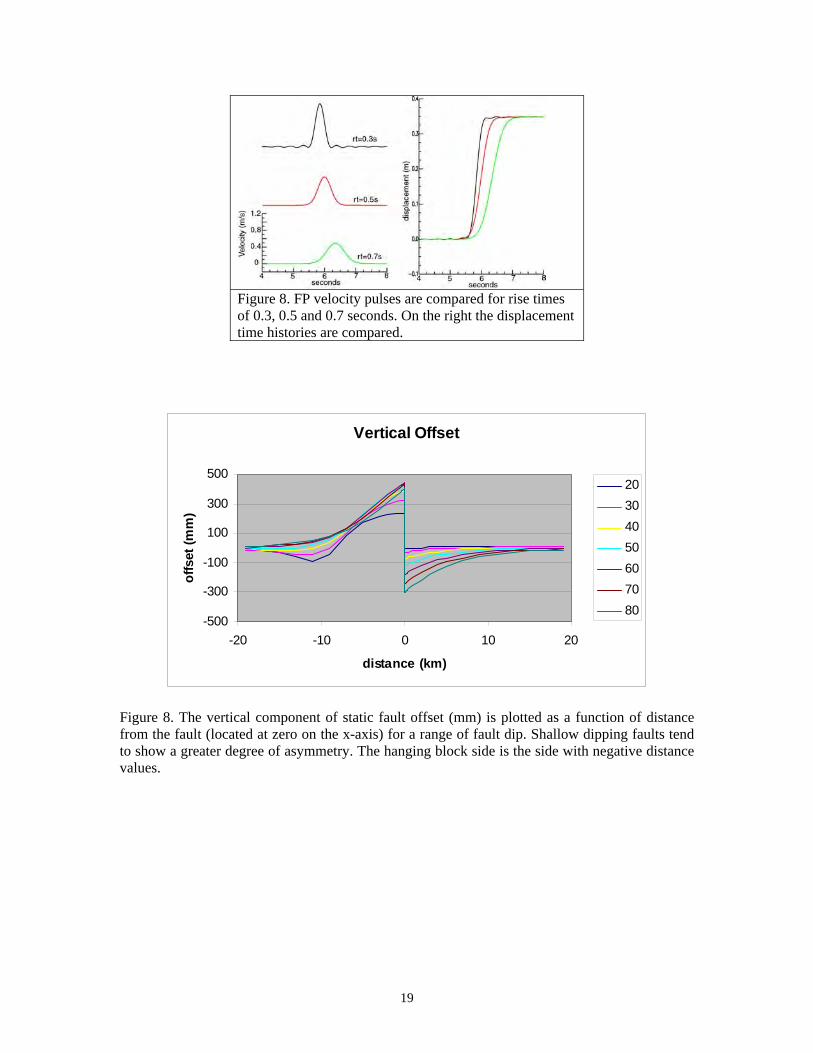
Figure 8. FP velocity pulses are compared for rise times of 0.3, 0.5 and 0.7 seconds. On the right the displacement time histories are compared.
Vertical Offset
-500
-300
-100
100
300
500
-20 -10 0 10 20
distance (km)
offs
et (m
m)
20 30 40 50 60 70 80
Figure 8. The vertical component of static fault offset (mm) is plotted as a function of distance from the fault (located at zero on the x-axis) for a range of fault dip. Shallow dipping faults tend to show a greater degree of asymmetry. The hanging block side is the side with negative distance values.
19
Fault Normal Offset
-600
-400
-200
0
200
400
600
-20 -10 0 10 20
distance (km)
offs
et (m
m)
20 30 40 50 60 70 80
Figure 9. The fault-normal component of static fault offset (mm) is plotted as a function of distance from the fault (located at zero on the x-axis) for a range of fault dip. Shallow dipping faults tend to show a greater degree of asymmetry. The hanging block side is the side with negative distance values.
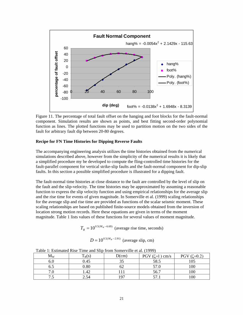
The results of these simulations are presented in terms of the percentage of total fault offset in Figures 10 and 11. This presentation may be used to specify the asymmetry of fault motions taking into account the dip of the fault for a pure reverse event. The simulation results are well fit by second-order polynomial functions, which can be used to determine the partitioning of motion for a fault of arbitrary dip between 20-80 degrees.
Vertical Component hang% = -0.0154x2 + 1.9205x + 1.5142
foot% = -0.0032x2 - 0.3739x + 8.9702
-60 -40 -20
0
20 40 60 80
0 20 40 60 80 100
dip (deg)
perc
enta
ge o
f fau
lt of
fset
hang% foot% Poly. (hang%) Poly. (foot%)
Figure 10. The percentage of total fault offset on the hanging and foot blocks for the vertical component. Simulation results are shown as points, and best fitting second-order polynomial function as lines. The plotted functions may be used to partition motion on the two sides of the fault for arbitrary fault dip between 20-80 degrees.
20
Fault Normal Component hang% = -0.0054x2 + 2.1429x - 115.63
foot% = -0.0138x2 + 1.6948x - 8.3139
-100 -80 -60 -40 -20
0 20 40 60
0 20 40 60 80 100
dip (deg)
perc
enta
ge o
f fau
lt of
fset
hang% foot% Poly. (hang%) Poly. (foot%)
Figure 11. The percentage of total fault offset on the hanging and foot blocks for the fault-normal component. Simulation results are shown as points, and best fitting second-order polynomial function as lines. The plotted functions may be used to partition motion on the two sides of the fault for arbitrary fault dip between 20-80 degrees.
Recipe for FN Time Histories for Dipping Reverse Faults
The accompanying engineering analysis utilizes the time histories obtained from the numerical simulations described above, however from the simplicity of the numerical results it is likely that a simplified procedure my be developed to compute the fling-controlled time histories for the fault-parallel component for vertical strike-slip faults and the fault-normal component for dip-slip faults. In this section a possible simplified procedure is illustrated for a dipping fault.
The fault-normal time histories at close distance to the fault are controlled by the level of slip on the fault and the slip-velocity. The time histories may be approximated by assuming a reasonable function to express the slip velocity function and using empirical relationships for the average slip and the rise time for events of given magnitude. In Somerville et al. (1999) scaling relationships for the average slip and rise time are provided as functions of the scalar seismic moment. These scaling relationships are based on published finite-source models obtained from the inversion of location strong motion records. Here these equations are given in terms of the moment magnitude. Table 1 lists values of these functions for several values of moment magnitude.
MW −6.69)TR = 100.5( (average rise time, seconds)
MW −2.91)D = 100.5( (average slip, cm)
Table 1: Estimated Rise Time and Slip from Somerville et al. (1999) MW TR(s) D(cm) PGV (ζ=1) cm/s PGV (ζ=0.2) 6.0 0.45 35 58.5 105 6.5 0.80 62 57.0 100 7.0 1.42 111 56.7 100 7.5 2.54 197 57.1 100
21
2D .
−tζ (TR / 4)The slip velocity function may be parameterized as s(t) = t e , where TR is the rise time.
This function has the favorable attributes of a smooth spectrum, and an adjustable high-frequency decay rate governed through the ζ parameter. When ζ=1 the function has a omega-2 high frequency decay rate and is the Brune source. For 0<ζ<1 the high-frequency decay rate is between 1/ω and 1/ω2, where ω is the angular frequency.
The slip velocity function is normalized by requiring that ∫ s(t)dt =
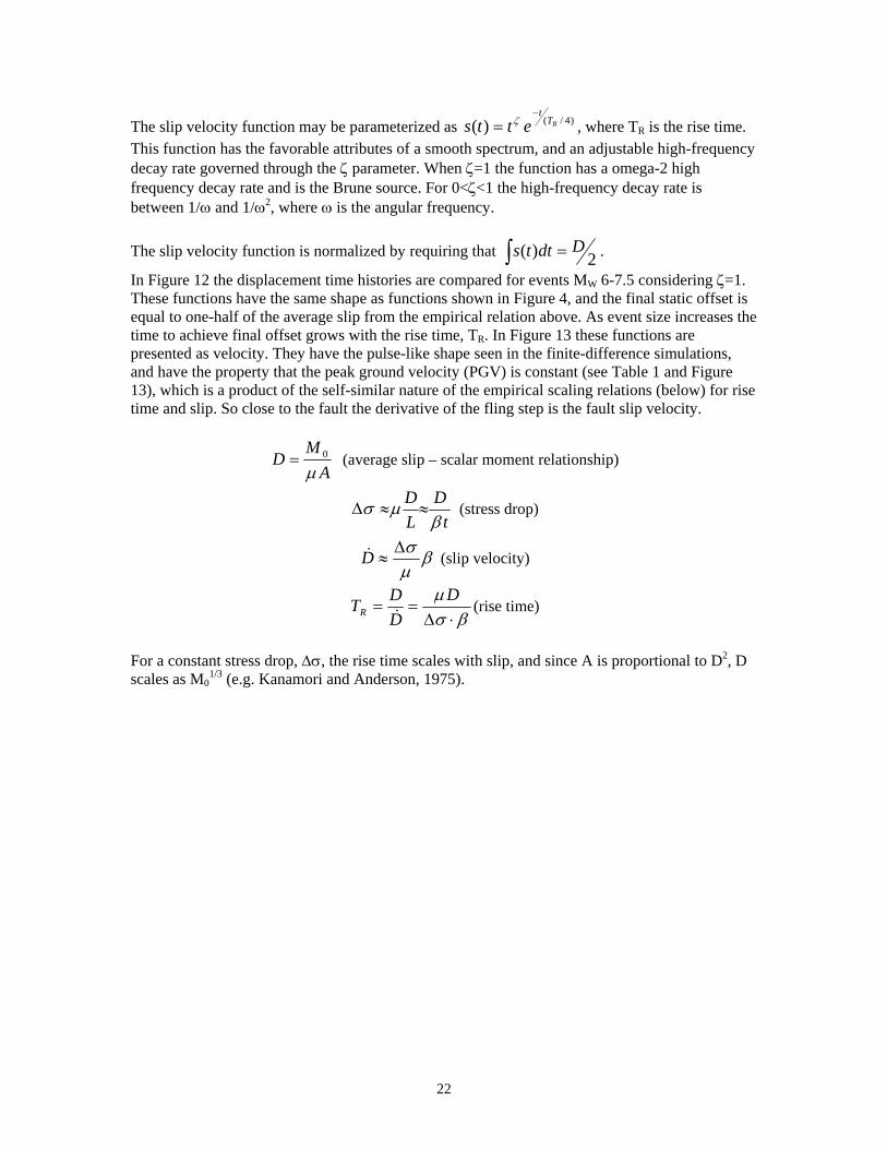
In Figure 12 the displacement time histories are compared for events MW 6-7.5 considering ζ=1. These functions have the same shape as functions shown in Figure 4, and the final static offset is equal to one-half of the average slip from the empirical relation above. As event size increases the time to achieve final offset grows with the rise time, TR. In Figure 13 these functions are presented as velocity. They have the pulse-like shape seen in the finite-difference simulations, and have the property that the peak ground velocity (PGV) is constant (see Table 1 and Figure 13), which is a product of the self-similar nature of the empirical scaling relations (below) for rise time and slip. So close to the fault the derivative of the fling step is the fault slip velocity.
M 0D = (average slip – scalar moment relationship) µ A
D D∆σ ≈µ ≈ (stress drop)
L β t ∆σD� ≈ β (slip velocity) µ
D µ DTR = = (rise time) �D ∆σ ⋅ β
For a constant stress drop, ∆σ, the rise time scales with slip, and since A is proportional to D2, D scales as M0
1/3 (e.g. Kanamori and Anderson, 1975).
22
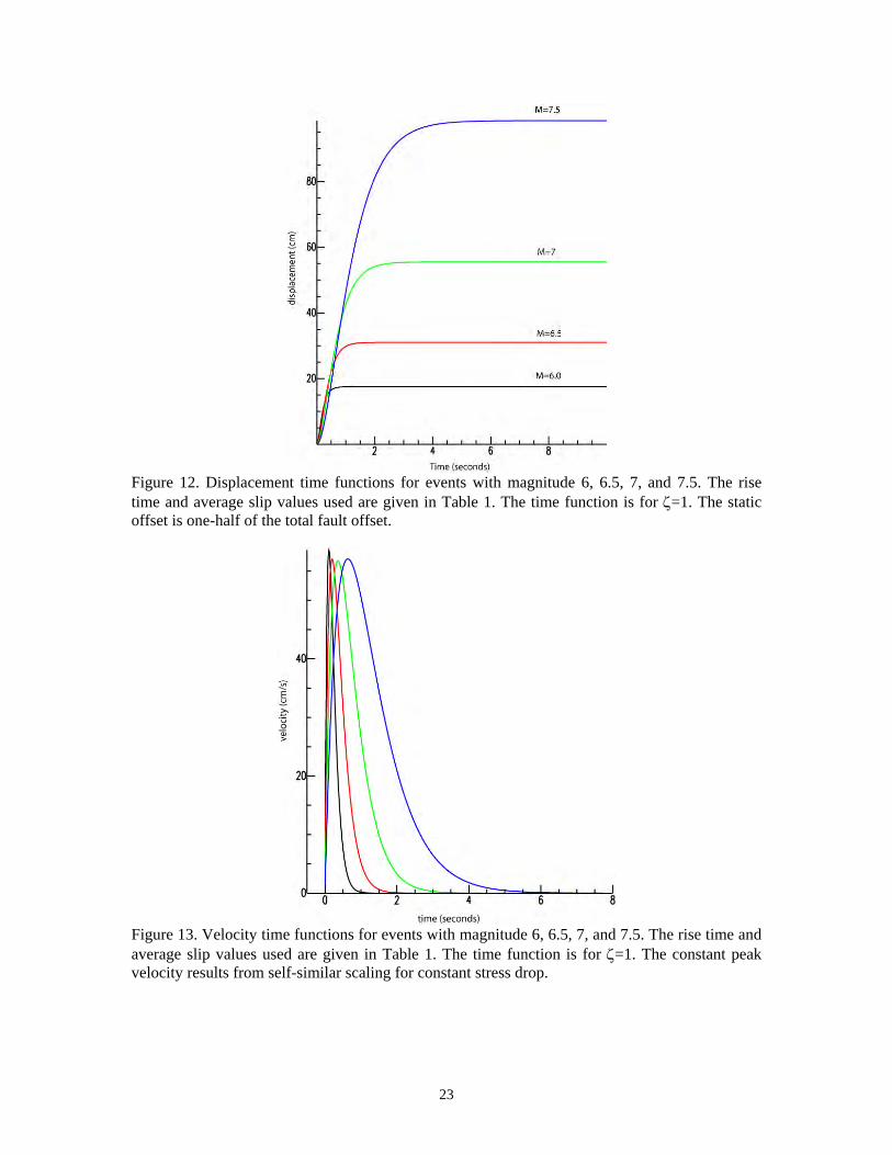
Figure 12. Displacement time functions for events with magnitude 6, 6.5, 7, and 7.5. The rise time and average slip values used are given in Table 1. The time function is for ζ=1. The static offset is one-half of the total fault offset.
Figure 13. Velocity time functions for events with magnitude 6, 6.5, 7, and 7.5. The rise time and average slip values used are given in Table 1. The time function is for ζ=1. The constant peak velocity results from self-similar scaling for constant stress drop.
23
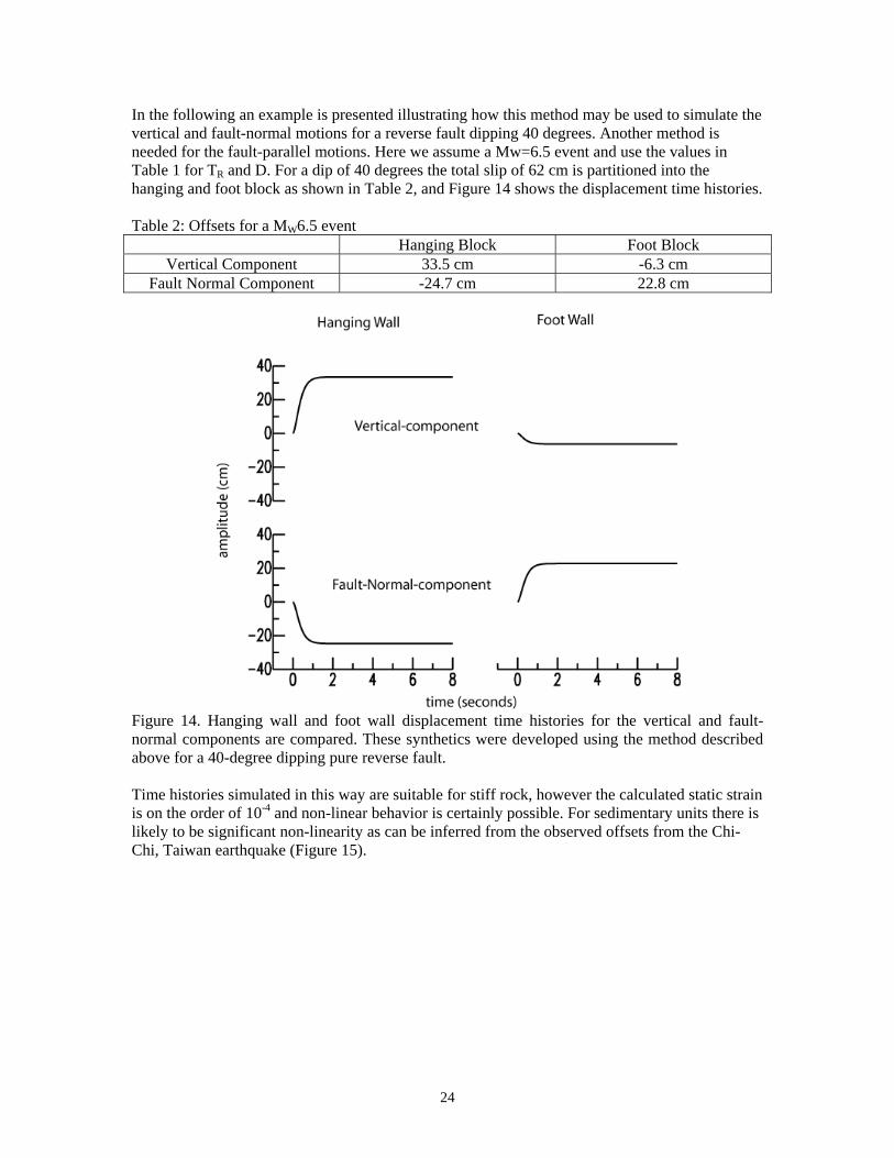
In the following an example is presented illustrating how this method may be used to simulate the vertical and fault-normal motions for a reverse fault dipping 40 degrees. Another method is needed for the fault-parallel motions. Here we assume a Mw=6.5 event and use the values in Table 1 for TR and D. For a dip of 40 degrees the total slip of 62 cm is partitioned into the hanging and foot block as shown in Table 2, and Figure 14 shows the displacement time histories.
Table 2: Offsets for a MW6.5 event Hanging Block Foot Block
Vertical Component 33.5 cm -6.3 cm Fault Normal Component -24.7 cm 22.8 cm
Figure 14. Hanging wall and foot wall displacement time histories for the vertical and fault-normal components are compared. These synthetics were developed using the method described above for a 40-degree dipping pure reverse fault.
Time histories simulated in this way are suitable for stiff rock, however the calculated static strain is on the order of 10-4 and non-linear behavior is certainly possible. For sedimentary units there is likely to be significant non-linearity as can be inferred from the observed offsets from the Chi-Chi, Taiwan earthquake (Figure 15).
24
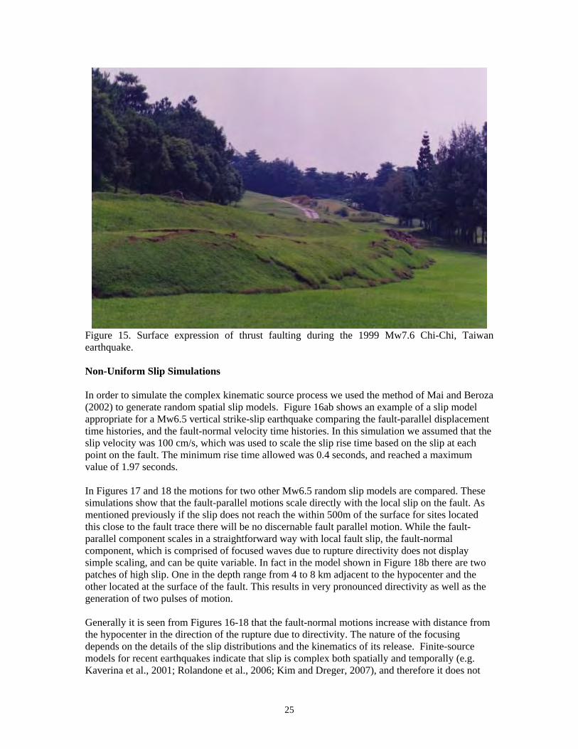
Figure 15. Surface expression of thrust faulting during the 1999 Mw7.6 Chi-Chi, Taiwan earthquake.
Non-Uniform Slip Simulations
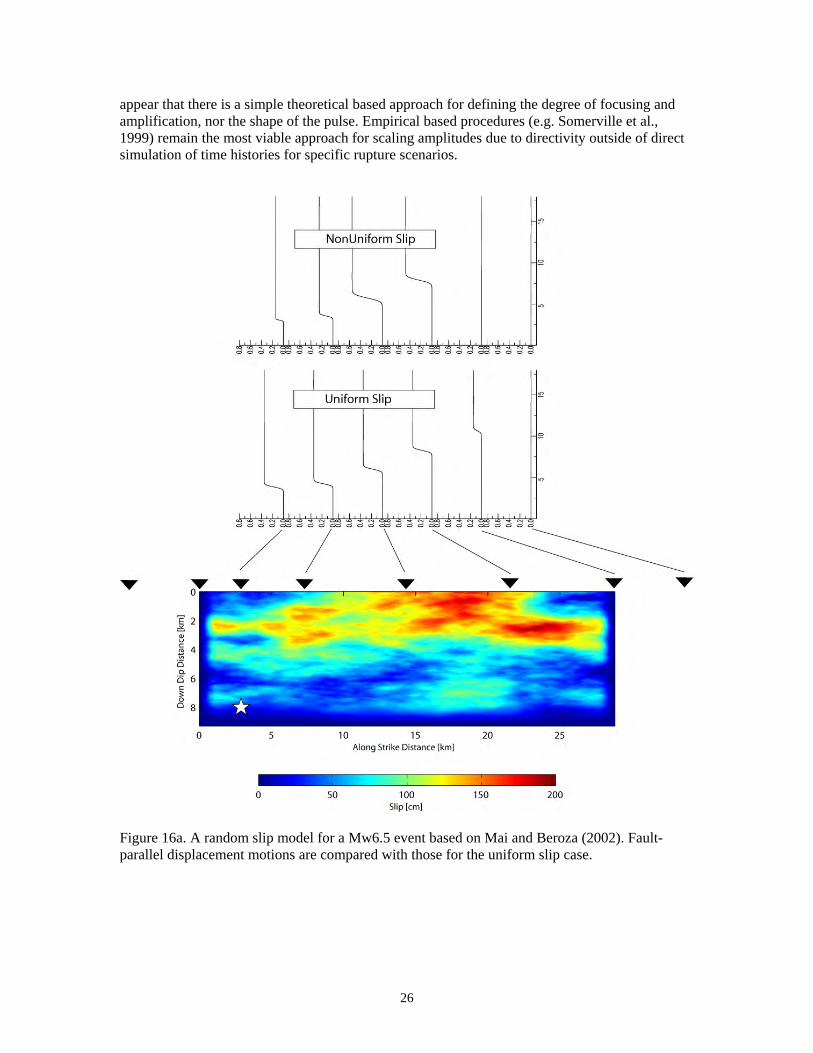
In order to simulate the complex kinematic source process we used the method of Mai and Beroza (2002) to generate random spatial slip models. Figure 16ab shows an example of a slip model appropriate for a Mw6.5 vertical strike-slip earthquake comparing the fault-parallel displacement time histories, and the fault-normal velocity time histories. In this simulation we assumed that the slip velocity was 100 cm/s, which was used to scale the slip rise time based on the slip at each point on the fault. The minimum rise time allowed was 0.4 seconds, and reached a maximum value of 1.97 seconds.
In Figures 17 and 18 the motions for two other Mw6.5 random slip models are compared. These simulations show that the fault-parallel motions scale directly with the local slip on the fault. As mentioned previously if the slip does not reach the within 500m of the surface for sites located this close to the fault trace there will be no discernable fault parallel motion. While the fault-parallel component scales in a straightforward way with local fault slip, the fault-normal component, which is comprised of focused waves due to rupture directivity does not display simple scaling, and can be quite variable. In fact in the model shown in Figure 18b there are two patches of high slip. One in the depth range from 4 to 8 km adjacent to the hypocenter and the other located at the surface of the fault. This results in very pronounced directivity as well as the generation of two pulses of motion.
Generally it is seen from Figures 16-18 that the fault-normal motions increase with distance from the hypocenter in the direction of the rupture due to directivity. The nature of the focusing depends on the details of the slip distributions and the kinematics of its release. Finite-source models for recent earthquakes indicate that slip is complex both spatially and temporally (e.g. Kaverina et al., 2001; Rolandone et al., 2006; Kim and Dreger, 2007), and therefore it does not
25
appear that there is a simple theoretical based approach for defining the degree of focusing and amplification, nor the shape of the pulse. Empirical based procedures (e.g. Somerville et al., 1999) remain the most viable approach for scaling amplitudes due to directivity outside of direct simulation of time histories for specific rupture scenarios.
Figure 16a. A random slip model for a Mw6.5 event based on Mai and Beroza (2002). Fault-parallel displacement motions are compared with those for the uniform slip case.
26
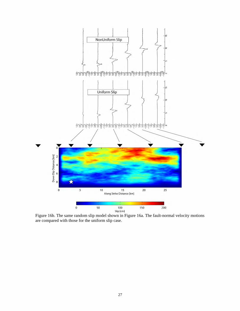
Figure 16b. The same random slip model shown in Figure 16a. The fault-normal velocity motions are compared with those for the uniform slip case.
27
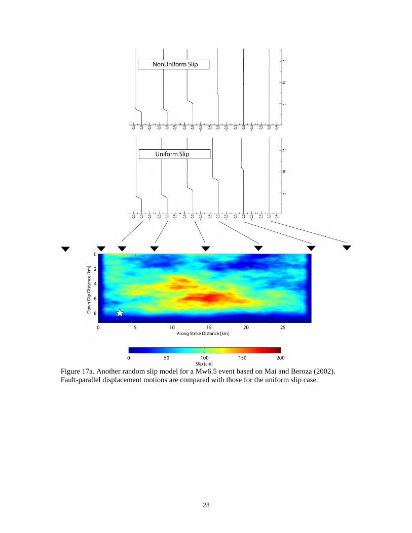
Figure 17a. Another random slip model for a Mw6.5 event based on Mai and Beroza (2002). Fault-parallel displacement motions are compared with those for the uniform slip case.
28
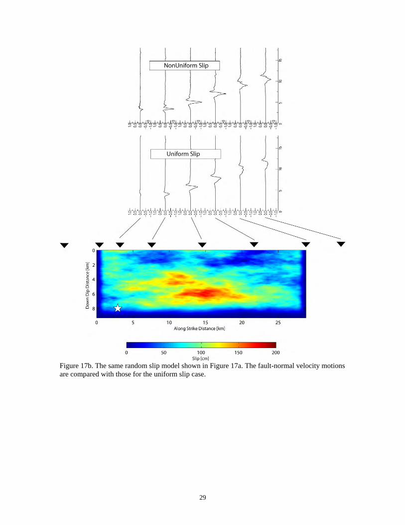
Figure 17b. The same random slip model shown in Figure 17a. The fault-normal velocity motions are compared with those for the uniform slip case.
29
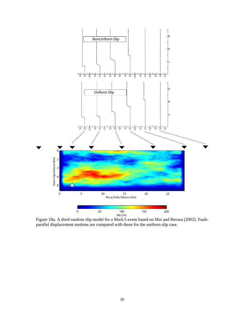
Figure 18a. A third random slip model for a Mw6.5 event based on Mai and Beroza (2002). Fault-parallel displacement motions are compared with those for the uniform slip case.
30
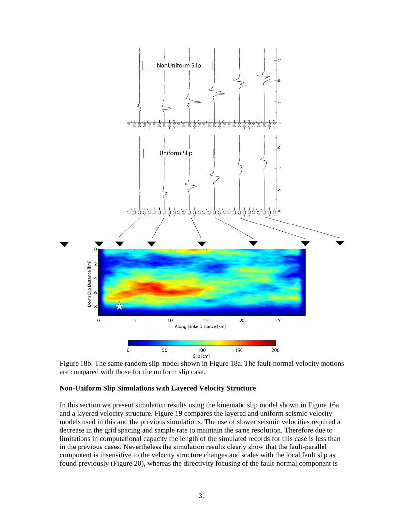
Figure 18b. The same random slip model shown in Figure 18a. The fault-normal velocity motions are compared with those for the uniform slip case.
Non-Uniform Slip Simulations with Layered Velocity Structure
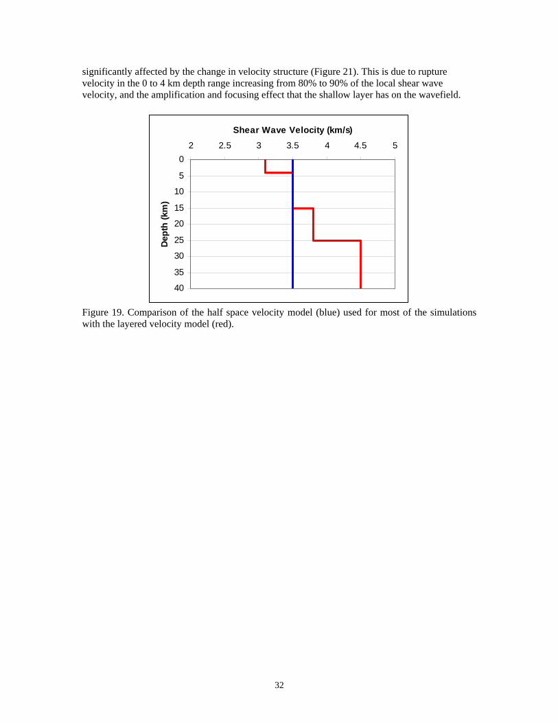
In this section we present simulation results using the kinematic slip model shown in Figure 16a and a layered velocity structure. Figure 19 compares the layered and uniform seismic velocity models used in this and the previous simulations. The use of slower seismic velocities required a decrease in the grid spacing and sample rate to maintain the same resolution. Therefore due to limitations in computational capacity the length of the simulated records for this case is less than in the previous cases. Nevertheless the simulation results clearly show that the fault-parallel component is insensitive to the velocity structure changes and scales with the local fault slip as found previously (Figure 20), whereas the directivity focusing of the fault-normal component is
31
significantly affected by the change in velocity structure (Figure 21). This is due to rupture velocity in the 0 to 4 km depth range increasing from 80% to 90% of the local shear wave velocity, and the amplification and focusing effect that the shallow layer has on the wavefield.
0
5
10
15
20
25
30
35
40
2 2.5 3 3.5 4 4.5 5
Shear Wave Velocity (km/s)
Dept
h (k
m)
Figure 19. Comparison of the half space velocity model (blue) used for most of the simulations with the layered velocity model (red).
32
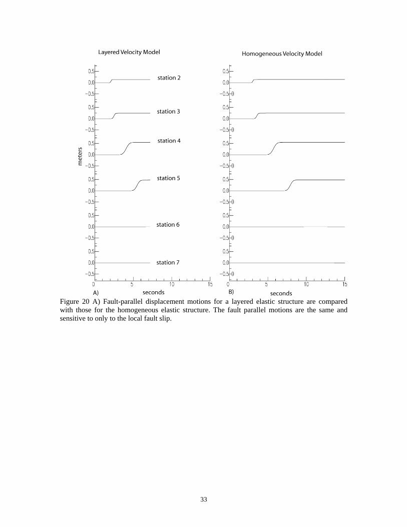
Figure 20 A) Fault-parallel displacement motions for a layered elastic structure are compared with those for the homogeneous elastic structure. The fault parallel motions are the same and sensitive to only to the local fault slip.
33
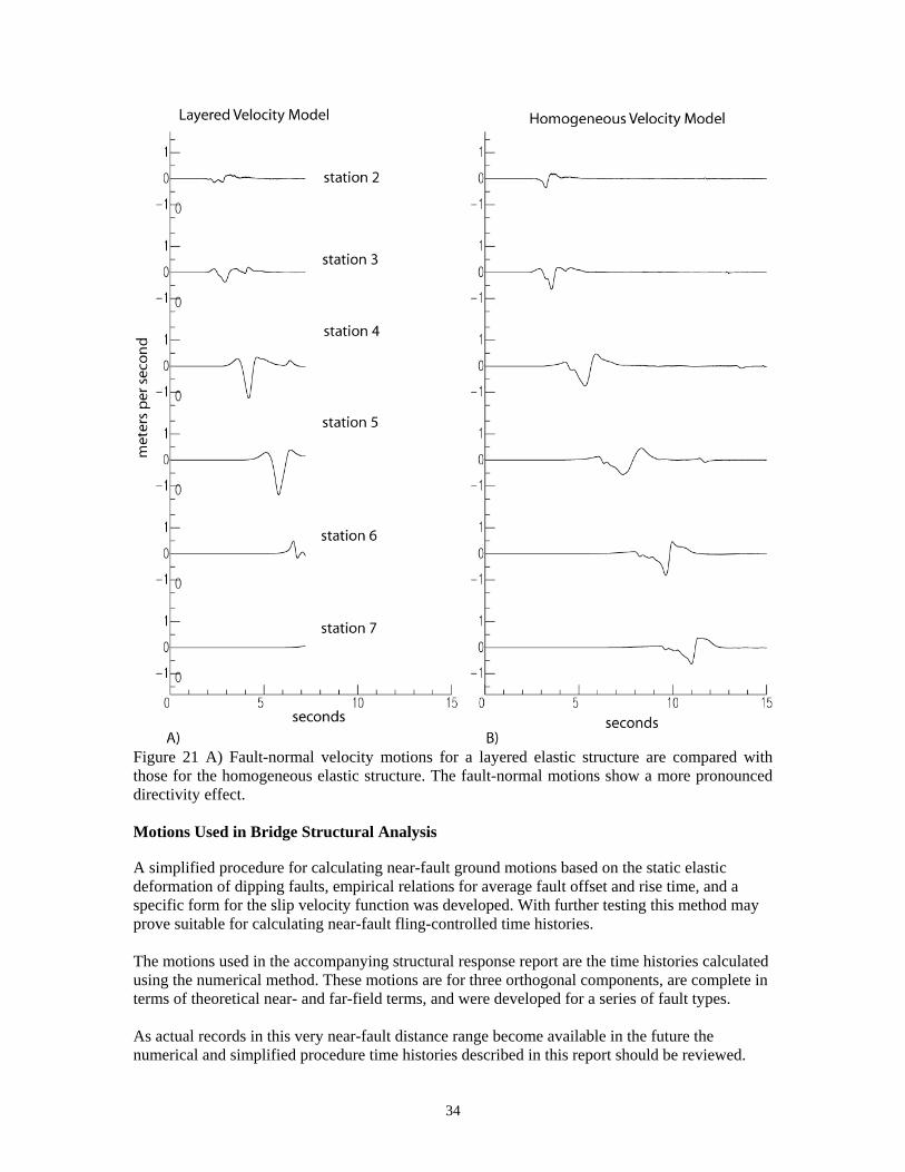
Figure 21 A) Fault-normal velocity motions for a layered elastic structure are compared with those for the homogeneous elastic structure. The fault-normal motions show a more pronounced directivity effect.
Motions Used in Bridge Structural Analysis
A simplified procedure for calculating near-fault ground motions based on the static elastic deformation of dipping faults, empirical relations for average fault offset and rise time, and a specific form for the slip velocity function was developed. With further testing this method may prove suitable for calculating near-fault fling-controlled time histories.
The motions used in the accompanying structural response report are the time histories calculated using the numerical method. These motions are for three orthogonal components, are complete in terms of theoretical near- and far-field terms, and were developed for a series of fault types.
As actual records in this very near-fault distance range become available in the future the numerical and simplified procedure time histories described in this report should be reviewed.
34
Conclusions
We have simulated near-fault time histories 15m from the fault for use in the analysis of fault-crossing bridges. These time histories are complete in terms of far- and near-field terms and therefore contain the effects of rupture directivity and fault fling. Rupture directivity produces strong displacement and velocity pulses that increase in amplitude in the direction of the rupture. The fling produces static offsets in displacement and single sided velocity pulses. At distances less than 100m both effects can be very strong.
In this study we have simulated motions for a range of fault types from vertical strike-slip to a 20-degree dipping thrust fault. The results of these uniform slip simulations show that the directivity and fling controlled waveforms occur on different components for each fault type. For a vertical strike-slip fault pronounced directivity is observed on the FN component, while nearly constant amplitude static offset in displacement and single-sided velocity pulses are observed on the FP component. In contrast, thrust type events show the static offset on the FN component with a weak directivity on the FP component, and also significant amplitude motions on the vertical component. Generally the results show that both static offsets and large amplitude velocity pulses need to be considered on all three components, and this is readily observed in the oblique rupture cases we considered.
For a vertical strike-slip fault the FN ground motions are the same on each side of the fault, whereas the FP component not surprisingly has equal amplitude but opposite static offset. The corresponding velocity pulses are the same on each side of the fault for the FN component, but opposite in sign on the FP component. This degree of symmetry disappears when the fault is dipping due to the unbounded free-surface. Motions on the hanging block side are larger due to the free-surface effect, and because a greater fraction of the fault surface is closer to the stations on the side of the fault that dips beneath the recording stations. Both the dynamic and static motions are observed to be larger on the hanging block. We present a method for specifying the asymmetry of motions for dipping reverse faults.
Across fault static motions also depend strongly on the depth of the top of the fault. If the fault breaks the surface the across fault motions are naturally a maximum. If the fault is at depth they are greatly reduced. We performed a simulation with the top of the fault at 500m and the results indicate that differential static motions close to the fault are negligible. This is also evident in the variable slip simulations.
The amount of directivity depends on the length of the ruptured fault between the hypocenter and the recording station, the slip distribution along the rupture path, and the rupture velocity. We also found that velocity structure also has a strong effect on the focusing of waves on the FN component. The strong velocity pulses due to fault fling are to first order sensitive to the local slip and slip rise time on the fault.
Most of the simulations were for a rupture velocity 80% of the shear-wave velocity. Simulations were also performed for the vertical strike-slip case with rupture velocities equal to 70% and 141% of the shear-wave speed. In these simulations the FP, or fling controlled motions were unchanged. There were differences to the FN, or directivity controlled motions in terms of waveshape and amplitude.
35
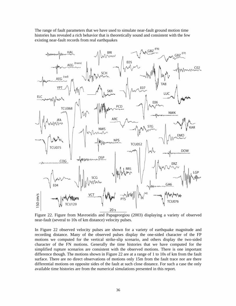
The range of fault parameters that we have used to simulate near-fault ground motion time histories has revealed a rich behavior that is theoretically sound and consistent with the few existing near-fault records from real earthquakes
Figure 22. Figure from Mavroeidis and Papageorgiou (2003) displaying a variety of observed near-fault (several to 10s of km distance) velocity pulses.
In Figure 22 observed velocity pulses are shown for a variety of earthquake magnitude and recording distance. Many of the observed pulses display the one-sided character of the FP motions we computed for the vertical strike-slip scenario, and others display the two-sided character of the FN motions. Generally the time histories that we have computed for the simplified rupture scenarios are consistent with the observed motions. There is one important difference though. The motions shown in Figure 22 are at a range of 1 to 10s of km from the fault surface. There are no direct observations of motions only 15m from the fault trace nor are there differential motions on opposite sides of the fault at such close distance. For such a case the only available time histories are from the numerical simulations presented in this report.
36
References
Aagaard, B. T., and T. Heaton (2004). Near-source ground motions from simulations of sustained intersonic and supersonic fault ruptures, Bull. Seism. Soc. Am., 94, 2064-2078.
Aagaard, B. T., J. F. Hall, and T. H. Heaton (2004). Effects of fault dip and slip rake angles on near-source ground motions: Why rupture directivity was minimal in the 1999 Chi-Chi, Taiwan, earthquake, Bull. Seism. Soc. Am., 94, 155-170.
Abrahamson, N. A. and W. J. Silva (1997). Epirical response spectral attenuation relations for shallow crustal earthquakes, Seism. Res. Lett., 68, 1, 94-127.
Bouchon, M., M. P. Bouin, H. Karabulut, M. N. Toksoz, M. Dietrich and A. Rosakis (2001). How fast is rupture during an earthquake? New insights from the 1999 Turkey earthquakes, Geophys. Res. Lett., 28, 2723-2726.
Bouchon, M., and M. Vallee (2003). Observation of long supershear rupture during the magntidue 8.1 Kuunlunshan earthquake, Science, 301, 824-826.
Chi, W.C., D. Dreger, and A. Kaverina (2001) Finite-source modeling of the 1999 Taiwan (Chi-Chi) earthquake derived from a dense strong-motion network, Dedicated issue on the Chi-Chi, Taiwan earthquake of 20 September 1999, Bull. Seism. Soc. Am., vol.91, no.5, pp.1144-1157.
Clayton, R. and B. Engquist (1977). Absorbing boundary conditions for acoustic and elastic wave equations, Bull. Seism. Soc. Am., 67, 1529-1540.
Dolenc, D., D. Dreger and S. Larsen (2005). Basin Structure Influences on the Propagation of Teleseismic Waves in the Santa Clara Valley, California, Bull. Seism. Soc. Am., 95, 1120.
Dreger, D. S., L. Gee, P. Lombard, M. H. Murray, and B. Romanowicz (2005). Rapid Finite-Source Analysis and Near-Fault Strong Ground Motions – Application to the 2003 Mw6.5 San Simeon and 2004 Mw6.0 Parkfield Earthquakes, Seism. Res. Lett. 76, 40-48.
Dunham, E. M. and R. J. Archuleta (2004). Evidence for a supershear transient during the 2002 Denali Fault earthquake, Bull. Seism. Soc. Am., 94, s256-s268.
Kanamori, H. K. and D. L. Anderson (1975). Theoretical basis of some empirical relations in seismology, Bull. Seism. Soc. Am. 65, 1073-1095.
Larsen, S. and C.A. Schultz (1995). ELAS3D: 2D/3D elastic finite-difference wave propagation code, Lawrence Livermore National Laboratory Technical Report No. UCRL-MA-121792, 19 pp.
Levander, A.R. (1988). Fourth-order finite-difference P-SV seismograms, Geophysics, 53, 1425-1436.
Mai, P. M. and G. C. Beroza (2002). A spatial random-field model to characterize complexity in earthquake slip, Journ. Geophys. Res., 107 (B11), 2308, doi:10.1029/2001JB000588.
Mavroeidis, G. P., and A. S. Papageorgiou (2003). A mathematical representation of near-fault ground motion, Bull. Seism. Soc. Am., 93, 1099-1131.
37
Okada, Y. (1992). Internal deformation due to shear and tensile faults in a half-space, Bull. Seism. Soc. Am., 82, 1018-1040.
Panning, M., D. Dreger and H. Tkalcic (2001). Near-source velocity structure and isotropic moment tensors: a case study of the Long Valley Caldera, Geophys. Res. Lett., 28, 1815-1818.
Rolandone, F., D. Dreger, M. Murray, and R. Burgmann (2006). Coseismic slip distribution of the 2003 Mw6.6 San Simeon earthquake, California, determined from GPS measurements and seismic waveform data, Geophys. Res. Lett., 33, L16315, doi:10.1029/2006GL027079.
Somerville, P. G., K. Irikura, R. Graves, S. Sawada, D. Wald, N. Abrahamson, Y. Iwasaki, T. Kagawa, N. Smith, and A. Kowada (1999). Characterizing crustal earthquake slip models for the prediction of strong ground motion, Seism. Res. Lett., 70, 59-80.
Stidham, C., M. Antolik, D. Dreger, S. Larsen, and B. Romanowicz (1999). Three-dimensional structure influences on the strong-motion wavefield of the 1989 Loma Prieta earthquake, Bull. Seism. Soc. Am., 89, 1184-1202.
Wells, D. L., and K. J. Coppersmith (1994) New empirical relationships among magnitude, rupture length, rupture width, rupture area, and surface displacement, Bull. Seism. Soc. Am., 84, 974-1002.
38
Related Documents

![SEISMIC PERFORMANCE ASSESSMENT OF HYBRID SELF- …icass2018.com/down/pdf/P-126.pdf · computer software OpenSees Ver.2.5 [21] and analyzed under near-fault earthquake ground motions.](https://static.cupdf.com/doc/110x72/5ead3bb0fc8b4968b130ac15/seismic-performance-assessment-of-hybrid-self-computer-software-opensees-ver25.jpg)