Nciplot Manual

1

�CIPLOT MA�UAL

A PROGRAM FOR PLOTTI�G �O�-COVALE�T

I�TERACTIO� REGIO�S

By Julia Contreras-García, Erin R. Johnson, S. Keinan and W. Yang

2

INDEX

1 Theoretical background ...................................................................................................................... 3

2 Installing the program ......................................................................................................................... 5

3 Running the program .......................................................................................................................... 5

4 The input ............................................................................................................................................. 5

5 The output .......................................................................................................................................... 7

6 Examples ............................................................................................................................................. 9

6.1 Plotting options ........................................................................................................................... 9

6.2 Number of files ......................................................................................................................... 10

6.3 SCF or promolecular? ................................................................................................................ 10

6.4 Choosing the interaction .......................................................................................................... 11

6.5 Protein-ligand interactions ....................................................................................................... 12

7 Using the VMD script ........................................................................................................................ 13

8 Advanced users ................................................................................................................................. 14

9 What went wrong? ........................................................................................................................... 14

9.1 Error messages .......................................................................................................................... 14

9.2 Other sources of problems ....................................................................................................... 15

10 Cite us ........................................................................................................................................... 15

11 Appendix: Geometry data ............................................................................................................. 15

1 Theoretical backgroundNCI (Non-Covalent Interactions) is a visualization index based on the density an

identification of non-covalent interactions. It is based on the peaks that appear in the reduced density

(RDG) at low densities. As highlighted in Figure

points in between molecules due to the annihilation of the density gradient at these points.

Figure 1. ρ(r), s(ρ) and NCI pieces in ben

When we plot the RDG as a function of the

between the monomer and dimer cases is the appearance of steep peaks at low density (Figure 1 c

we search for the points in 3D space

(supra)molecular complex. These interactions correspond to both favorable and unfavorable interactions. In

order to differentiate between them

implemented. This value is able to characterize the strength of the interaction by means of the densi

curvature thanks to the sign of the second eigenvalue (see Ref. [1] for a th

Theoretical background Covalent Interactions) is a visualization index based on the density and its derivatives. It enables

covalent interactions. It is based on the peaks that appear in the reduced density

(RDG) at low densities. As highlighted in Figures 1a-b, there is a crucial change in the RDG at the critical

points in between molecules due to the annihilation of the density gradient at these points.

) and NCI pieces in benzene monomer and benzene di

en we plot the RDG as a function of the density across a molecule, we see that the main difference

er cases is the appearance of steep peaks at low density (Figure 1 c

we search for the points in 3D space giving rise to these peaks, non covalent regions clearly appear in the

(supra)molecular complex. These interactions correspond to both favorable and unfavorable interactions. In

order to differentiate between them, the sign of the second density Hessian eigenvalue times the density is

implemented. This value is able to characterize the strength of the interaction by means of the densi

thanks to the sign of the second eigenvalue (see Ref. [1] for a thorough explanation of the physics

3

d its derivatives. It enables

covalent interactions. It is based on the peaks that appear in the reduced density gradient

, there is a crucial change in the RDG at the critical

points in between molecules due to the annihilation of the density gradient at these points.

onomer and benzene dimer

density across a molecule, we see that the main difference

er cases is the appearance of steep peaks at low density (Figure 1 c-d). When

giving rise to these peaks, non covalent regions clearly appear in the

(supra)molecular complex. These interactions correspond to both favorable and unfavorable interactions. In

eigenvalue times the density is

implemented. This value is able to characterize the strength of the interaction by means of the density, and its

orough explanation of the physics

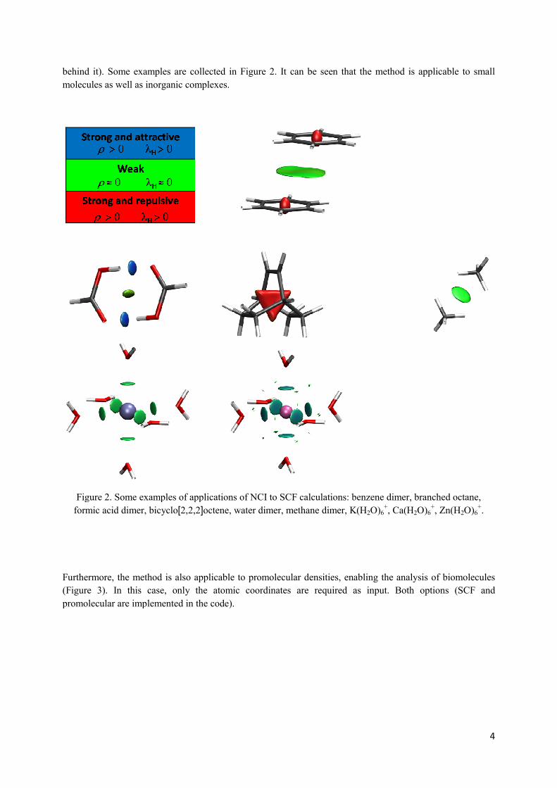
behind it). Some examples are collected in Figure 2.

molecules as well as inorganic complexes.

Figure 2. Some examples of applications

formic acid dimer, bicyclo[2,2,2]

Furthermore, the method is also applicable to promolecular densities,

(Figure 3). In this case, only the atomic coordinates are required as input. Both options (SCF and

promolecular are implemented in the code).

Some examples are collected in Figure 2. It can be seen that the method i

molecules as well as inorganic complexes.

Figure 2. Some examples of applications of NCI to SCF calculations: benzene dimer, branched octane,

]octene, water dimer, methane dimer, K(H2O)6+, Ca(H

Furthermore, the method is also applicable to promolecular densities, enabling the analysis of biomolecules

this case, only the atomic coordinates are required as input. Both options (SCF and

promolecular are implemented in the code).

4

It can be seen that the method is applicable to small

er, branched octane,

, Ca(H2O)6+, Zn(H2O)6

+.

enabling the analysis of biomolecules

this case, only the atomic coordinates are required as input. Both options (SCF and

Figure 3. Promolecular

2 Installing the programThe code has been assembled for an easy, use

code, so that no Makefile is required. For the moment, compilation with ifort is required under the following

command:

ifort nciplot.f -o nciplot

This will create the executable nciplot

3 Running the programThe code is invoked as follows:

nciplot.x input.file [output.file]

Alternatively, the repository is provided with an statically linked compilation which should work in most

linux machines (nciplot.x)

4 The input The input is keyword oriented, free-

The following coding is used for variables:

• r stands for real.

• x,y,z stand for positions in space (real)

• n stands for integer

Figure 3. Promolecular applications: α-helix, β-sheet, DNA

Installing the program been assembled for an easy, user-friendly compilation. All subroutines are collected in the same

code, so that no Makefile is required. For the moment, compilation with ifort is required under the following

o nciplot.x

nciplot.x

Running the program

input.file [output.file]

Alternatively, the repository is provided with an statically linked compilation which should work in most

-format, and the output is meant to be self-contained.

The following coding is used for variables:

stand for positions in space (real)

5

friendly compilation. All subroutines are collected in the same

code, so that no Makefile is required. For the moment, compilation with ifort is required under the following

Alternatively, the repository is provided with an statically linked compilation which should work in most

contained.

6

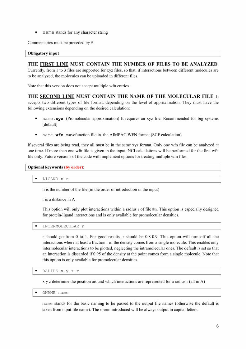
• name stands for any character string

Commentaries must be preceded by #

Obligatory input

THE FIRST LI�E MUST CO�TAI� THE �UMBER OF FILES TO BE A�ALYZED.

Currently, from 1 to 3 files are supported for xyz files, so that, if interactions between different molecules are

to be analyzed, the molecules can be uploaded in different files.

Note that this version does not accept multiple wfn entries.

THE SECO�D LI�E MUST CO�TAI� THE �AME OF THE MOLECULAR FILE. It

accepts two different types of file format, depending on the level of approximation. They must have the

following extensions depending on the desired calculation:

• name.xyz (Promolecular approximation) It requires an xyz file. Recommended for big systems

[default]

• name.wfn wavefunction file in the AIMPAC WFN format (SCF calculation)

If several files are being read, they all must be in the same xyz format. Only one wfn file can be analyzed at

one time. If more than one wfn file is given in the input, NCI calculations will be performed for the first wfn

file only. Future versions of the code with implement options for treating multiple wfn files.

Optional keywords (by order):

• LIGAND n r

n is the number of the file (in the order of introduction in the input)

r is a distance in A

This option will only plot interactions within a radius r of file #n. This option is especially designed

for protein-ligand interactions and is only available for promolecular densities.

• INTERMOLECULAR r

r should go from 0 to 1. For good results, r should be 0.8-0.9. This option will turn off all the

interactions where at least a fraction r of the density comes from a single molecule. This enables only

intermolecular interactions to be plotted, neglecting the intramolecular ones. The default is set so that

an interaction is discarded if 0.95 of the density at the point comes from a single molecule. Note that

this option is only available for promolecular densities.

• RADIUS x y z r

x y z determine the position around which interactions are represented for a radius r (all in A)

• ONAME name

name stands for the basic naming to be passed to the output file names (otherwise the default is

taken from input file name). The name introduced will be always output in capital letters.

7

• OUTPUT n

n is an integer running from 1 to 3.

o 1 will only print the .dat file

o 2 will only print the .cube files

o 3 will print all three output files [default]

• CUBE x0 y0 z0 x1 y1 z1

This option will set the cube within which NCI is analyzed as going from the Cartesian coordinate

(x0,y0,z0) to (x1,y1,z1).

The default is produced in terms of molecular coordinates. In order to ensure a correct cube in planar

or linear cases, a minimum distance of +/- 2a.u. is added to the axes in all directions.

• INCREMENTS r1 r2 r3

This option sets the increments along the x,y,z directions of the cube (atomic units). The default is

set to 0.1,0.1,0.1

• CUTOFFS r1 r2

Density (r1) and RDG (r2) cutoffs used in creating the dat file. The default density cutoff is set to

0.2. The RDG cutoff depends on the level of calculation:

o In the promolecular case it is set to 1.0.

o In the scf case it is set to 2.0.

• CUTPLOT r1 r2

Density (r1) and RDG (r2) cutoffs used when creating the cube files. r1 will set the cutoff for both

the density and the RDG to be registered in the cube files, whereas r2 will be used in the VMD script

for the plotting of isosurfaces. The default values are:

o In the promolecular case: r1=0.07, r2=0.3.

o In the SCF case: r1=0.05, r2=0.5.

5 The output

The output (may) consist of 4 files:

• name.dat file collects rho vs RDG (OUTPUT= 1 or 3)

8

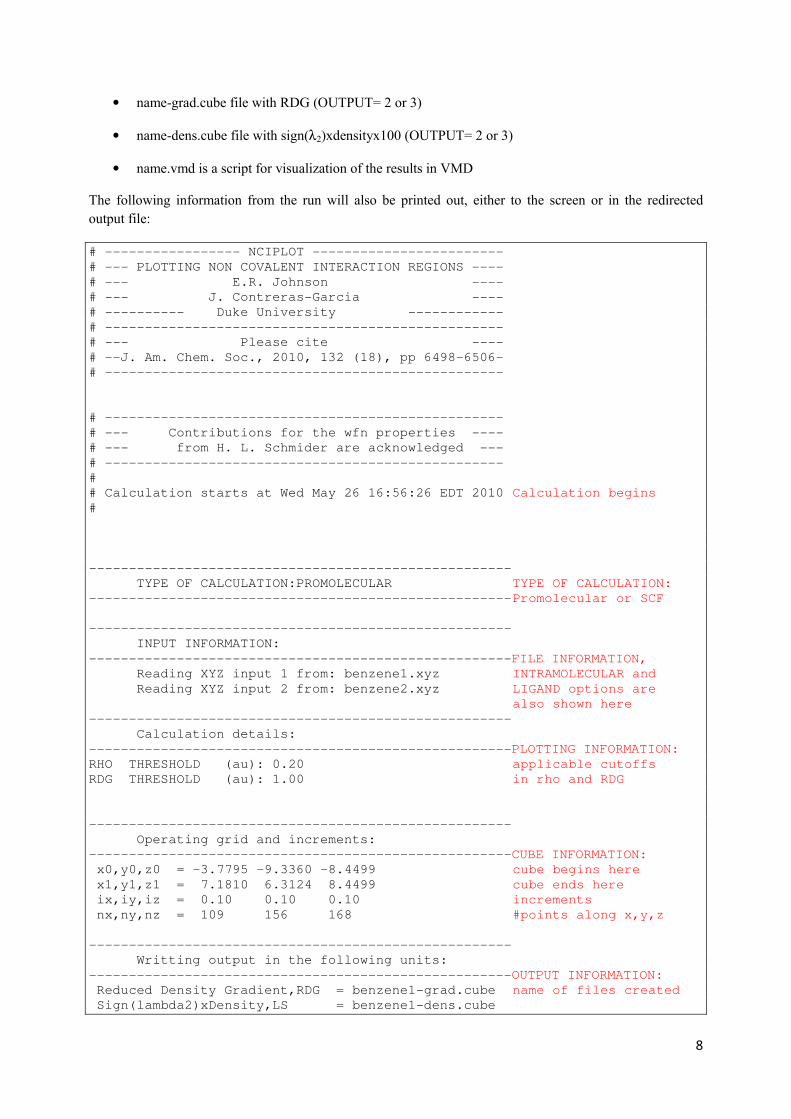
• name-grad.cube file with RDG (OUTPUT= 2 or 3)

• name-dens.cube file with sign(λ2)xdensityx100 (OUTPUT= 2 or 3)

• name.vmd is a script for visualization of the results in VMD

The following information from the run will also be printed out, either to the screen or in the redirected

output file:

# ----------------- NCIPLOT ------------------------

# --- PLOTTING NON COVALENT INTERACTION REGIONS ----

# --- E.R. Johnson ----

# --- J. Contreras-Garcia ----

# ---------- Duke University ------------

# --------------------------------------------------

# --- Please cite ----

# --J. Am. Chem. Soc., 2010, 132 (18), pp 6498-6506-

# --------------------------------------------------

# --------------------------------------------------

# --- Contributions for the wfn properties ----

# --- from H. L. Schmider are acknowledged ---

# --------------------------------------------------

#

# Calculation starts at Wed May 26 16:56:26 EDT 2010 Calculation begins

#

-----------------------------------------------------

TYPE OF CALCULATION:PROMOLECULAR TYPE OF CALCULATION:

----------------------------------------------------- Promolecular or SCF

-----------------------------------------------------

INPUT INFORMATION:

-----------------------------------------------------FILE INFORMATION,

Reading XYZ input 1 from: benzene1.xyz INTRAMOLECULAR and

Reading XYZ input 2 from: benzene2.xyz LIGAND options are

also shown here

-----------------------------------------------------

Calculation details:

-----------------------------------------------------PLOTTING INFORMATION:

RHO THRESHOLD (au): 0.20 applicable cutoffs

RDG THRESHOLD (au): 1.00 in rho and RDG

-----------------------------------------------------

Operating grid and increments:

-----------------------------------------------------CUBE INFORMATION:

x0,y0,z0 = -3.7795 -9.3360 -8.4499 cube begins here

x1,y1,z1 = 7.1810 6.3124 8.4499 cube ends here

ix,iy,iz = 0.10 0.10 0.10 increments

nx,ny,nz = 109 156 168 #points along x,y,z

-----------------------------------------------------

Writting output in the following units:

-----------------------------------------------------OUTPUT INFORMATION:

Reduced Density Gradient,RDG = benzene1-grad.cube name of files created

Sign(lambda2)xDensity,LS = benzene1-dens.cube

9

LS x RDG = benzene1.dat

VMD script = benzene1.vmd

-----------------------------------------------------

#----------------------------------------------- RUN INFORMATION:

#*** timer: calls and timing

#***

#*** -pid----name-----tottime-------pcalls--popen-

#*** 1 _main 76.720 1 F

#*** 2 _read 0.000 2 F

#*** 3 _prop 7.650 5713344 F

#*** 4 _eig 0.000 2856672 F

#*** 5 _dat 19.810 2856672 F

#*** 6 _cube 26.140 2856672 F

#***

#

# Calculation ends at Wed May 26 16:57:44 EDT 2010 CALCULATION ENDS

#

# Normal termination

#

6 Examples In all cases 3D pictures have been obtained by directly applying the VMD script from the calculation. The

lines defining the cube edges have also been highlighted when appropriate. Geometries used are collected in

the Appendix.

6.1 Plotting options

1

benzene.xyz

OUTPUT 2

CUBE -0.7 -9. -9. 0.7 9. 9.

INCREMENTS 0.2 0.2 0.2

CUTOFFS 0.05 0.27

6.2 Number of files

In this case, different options are possible. If

either introduce the molecules in a unique file (Option A

Option A

1

BenzeneDimer.xyz

In both cases we will obtain the same result

6.3 SCF or promolecular

The type of run (SCF or promolecular) is chosen from the

and wfn for scf. In both cases the visualization results are very similar. The main changes occur in the

cutoffs values. Figure 5 shows the results for different

be seen that RDG moves to higher values, and peaks shift toward more negative values

used.

Figure 5.

In this case, different options are possible. If we want to obtain all the interactions in the complex, we can

cules in a unique file (Option A) or separately (Option B):

Option B

2

benzene1.xyz

benzene2.xyz

In both cases we will obtain the same results:

Figure 4.

promolecular?

The type of run (SCF or promolecular) is chosen from the extension of the input files: xyz for promolecular

In both cases the visualization results are very similar. The main changes occur in the

cutoffs values. Figure 5 shows the results for different intramolecular and intermolecular interacti

be seen that RDG moves to higher values, and peaks shift toward more negative values

10

we want to obtain all the interactions in the complex, we can

extension of the input files: xyz for promolecular

In both cases the visualization results are very similar. The main changes occur in the

molecular and intermolecular interactions. It can

be seen that RDG moves to higher values, and peaks shift toward more negative values, if the scf density is

11

6.4 Choosing the interactions i. Appropriate choice of the cube boundaries enables the user to choose individual interactions (Input

Option C).

ii. It is also possible to select the interactions in terms of their strength by an appropriate choice of

cutoff parameters (Input Option D)

iii. To analyze only intermolecular interactions, the INTERMOLECULAR keyword should be used (Input

Option E).

iv. To analyze only interactions close to a given molecule, the LIGAND or RADIUS keywords can be

used (Input Options A and F).

Option C

1

formicaciddimmer.xyz

CUBE 1. -2. -1. 3. 2. 1.

Option D

1

formicaciddimmer.xyz

CUTOFFS 0.01 1.

Option E

2

benzene1.xyz

benzene2.xyz

INTERMOLECULAR

Option F

2

benzene1.xyz

benzene2.xyz

RADIUS -1.8 0.8 0.0 1.0

In order to choose appropriate cutoffs, it is possible to first make a run with OUTPUT=1, so that only the .dat

file is printed out. Plotting the results, with a program such as gnuplot, will help in choosing

values. A second run can then be made with OUTPUT=2 and using the PLOTCUT keyword

obtain the cube files:

Run #1

1

formicaciddimmer.xyz

OUTPUT 1

6.5 Protein-ligand interactionsOption D is especially designed for studying inclusion complexes and protein

small molecule fits into a cavity, and we want to understand the interactions with the active site. Here we

have an example:

cutoffs, it is possible to first make a run with OUTPUT=1, so that only the .dat

Plotting the results, with a program such as gnuplot, will help in choosing

can then be made with OUTPUT=2 and using the PLOTCUT keyword

Run #2

1

formicaciddimmer.xyz

CUTOFFS 0.01 1.

ligand interactions Option D is especially designed for studying inclusion complexes and protein-ligand interactions, where a

molecule fits into a cavity, and we want to understand the interactions with the active site. Here we

12

cutoffs, it is possible to first make a run with OUTPUT=1, so that only the .dat

Plotting the results, with a program such as gnuplot, will help in choosing the cutoff

can then be made with OUTPUT=2 and using the PLOTCUT keyword, in order to

formicaciddimmer.xyz

ligand interactions, where a

molecule fits into a cavity, and we want to understand the interactions with the active site. Here we

2

protein.xyz

ligand.xyz

LIGAND 2 4.0

7 Using the VMD scriptThe program generates a script for visualization of the results under the

loaded in VMD. After entering the working directory, the script

with a RDG cutoff as specified by the keyword

The script is as follows:

#!/usr/local/bin/vmd

# VMD script written by save_state $Revision: 1.41 $

# VMD version: 1.8.6

set viewplist

set fixedlist

# Display settings

display projection Orthographic

display nearclip set 0.000000

# load new molecule

mol new name-dens.cube type cube first 0 last

autobonds 1 waitfor all

mol addfile name-grad.cube

autobonds 1 waitfor all

#

# representation of the atoms

protein.xyz

ligand.xyz

LIGAND 2 4.0 ligand is file #2=ligand.xyz and we take

intermolecular interactions around it at <4A

Using the VMD script The program generates a script for visualization of the results under the name.vmd. This script can be

. After entering the working directory, the script will automatically generate an NCI picture

ified by the keyword PLOTCUT (otherwise, a default is used).

# VMD script written by save_state $Revision: 1.41 $

# VMD version: 1.8.6

set viewplist

set fixedlist

# Display settings

display projection Orthographic

display nearclip set 0.000000

# load new molecule

type cube first 0 last -1 step 1 filebonds 1

grad.cube type cube first 0 last -1 step 1 filebonds 1

# representation of the atoms

13

. This script can be

will automatically generate an NCI picture

(otherwise, a default is used).

1 step 1 filebonds 1

1 step 1 filebonds 1

14

mol delrep 0 top

mol representation CPK 1.000000 0.300000 118.000000 131.000000

mol color Name

mol selection {all}

mol material Opaque

mol addrep top

#

# add representation of the surface

mol representation Isosurface 0.30000 1 0 0 1 1

mol color Volume 0

mol selection {all}

mol material Opaque

mol addrep top

mol selupdate 1 top 0

mol colupdate 1 top 0

mol scaleminmax top 1 -4.000000 4.000000

mol smoothrep top 1 0

mol drawframes top 1 {now}

color scale method BGR

set colorcmds {{color Name {C} gray}}

#some more

In case the user wants to change it, the main options have been highlighted in red:

• name-dens.cube: name of the density cube file

• name-dens.cube: name of the gradient cube file

• 0.30000: value of RDG isosurface

• -4.000000 4.000000 where this is 100 times the value of rhoplot

8 Advanced users Here is a list of variables and parameters that can be internally tuned if desired:

PARAMETER DEFAULT MEA�I�G

��UCM2 10000 Maximum # of atoms (PROMOL)

��UCM 500 Maximum # of atoms (SCF)

�PRIM 10000 Maximum # of primitives (SCF)

�MOM 1000 Maximum # of orbitals (SCF)

MFILE 3 Maximum # of input files

9 What went wrong?

9.1 Error messages

• REQUESTED FILE DOES NOT EXIST

One of the input files does not exist in the directory

• TOO MANY ATOMS IN THE LIST, TRY DELETING NON INTERACTING ATOMS

The number of atoms is greater than allowed (Check NNUCM or NNUCM2)

• POWER L=X NOT SUPPORTED or TYPE X NOT ALLOWED

Orbital types supported are: s,sp and p

• PROBLEM READING ATOM TYPES

The format of the input file is not correct and the program is not reading all of the atoms

15

9.2 Other sources of problems

• Of course, units: the program deals with units automatically, but beware of input transformation.

xyz files are in A and wfn files are in au!!!

• Atomic densities for PROMOLECULAR calculations are only implemented for the atoms in the

first three row of the periodic table, H-Ar.

• Where is my data? Check the cutoffs, you might be discarding all your points.

• The VMD script is not working:

o The working directory should be the same that contains the script and the files

o The name of the files should be less than 40 characters long

10 Cite us

Erin R. Johnson, Shahar Keinan, Paula Mori-Sánchez, Julia Contreras-García, Aron J. Cohen, and Weitao

Yang, J. Am. Chem. Soc., 2010, 132 , pp 6498–6506

11 Appendix: Geometry data

benzene1:

C -1.800000 0.800000 1.391500

C -1.800000 -0.405074 0.695750

C -1.800000 -0.405074 -0.695750

C -1.800000 0.800000 -1.391500

C -1.800000 2.005074 -0.695750

C -1.800000 2.005074 0.695750

H -1.800000 0.800000 2.471500

H -1.800000 -1.340382 1.235750

H -1.800000 -1.340382 -1.235750

H -1.800000 0.800000 -2.471500

H -1.800000 2.940382 -1.235750

H -1.800000 2.940382 1.235750

benzene 2:

C 1.800000 -0.800000 1.391500

C 1.800000 0.405074 0.695750

C 1.800000 0.405074 -0.695750

C 1.800000 -0.800000 -1.391500

C 1.800000 -2.005074 -0.695750

C 1.800000 -2.005074 0.695750

H 1.800000 -0.800000 2.471500

H 1.800000 1.340382 1.235750

H 1.800000 1.340382 -1.235750

H 1.800000 -0.800000 -2.471500

H 1.800000 -2.940382 -1.235750

H 1.800000 -2.940382 1.235750

Benzene Dimer:

16

C -1.800000 0.800000 1.391500

C -1.800000 -0.405074 0.695750

C -1.800000 -0.405074 -0.695750

C -1.800000 0.800000 -1.391500

C -1.800000 2.005074 -0.695750

C -1.800000 2.005074 0.695750

H -1.800000 0.800000 2.471500

H -1.800000 -1.340382 1.235750

H -1.800000 -1.340382 -1.235750

H -1.800000 0.800000 -2.471500

H -1.800000 2.940382 -1.235750

H -1.800000 2.940382 1.235750

C 1.800000 -0.800000 1.391500

C 1.800000 0.405074 0.695750

C 1.800000 0.405074 -0.695750

C 1.800000 -0.800000 -1.391500

C 1.800000 -2.005074 -0.695750

C 1.800000 -2.005074 0.695750

H 1.800000 -0.800000 2.471500

H 1.800000 1.340382 1.235750

H 1.800000 1.340382 -1.235750

H 1.800000 -0.800000 -2.471500

H 1.800000 -2.940382 -1.235750

H 1.800000 -2.940382 1.235750

Formic acid dimer:

C -.120234 1.914070 .000000

H -.167295 3.007018 .000000

O -1.121857 1.220982 .000000

O 1.121857 1.480489 .000000

H 1.127582 .489024 .000000

O 1.121857 -1.220982 .000000

C .120234 -1.914070 .000000

O -1.121857 -1.480489 .000000

H -1.127582 -.489024 .000000

H .167295 -3.007018 .000000