NBER WORKING PAPER SERIES WHEN DO FIRMS GO ...

NBER WORKING PAPER SERIES

WHEN DO FIRMS GO GREEN? COMPARING COMMAND AND CONTROL REGULATIONS WITH PRICE INCENTIVES IN INDIA

Ann HarrisonBenjamin Hyman

Leslie MartinShanthi Nataraj

Working Paper 21763http://www.nber.org/papers/w21763

NATIONAL BUREAU OF ECONOMIC RESEARCH1050 Massachusetts Avenue

Cambridge, MA 02138November 2015, Revised October 2019

We are grateful to Michele De Nevers, Rema Hanna, Gil Metcalf, David Popp and seminar participants at Harvard Business School, the University of Hawaii, the Wharton International Lunch, Johns Hopkins SAIS, and the Indian School of Business for helpful comments and suggestions. We also thank Michael Greenstone and Rema Hanna for generously providing us with city-level pollutant data for India, and acknowledge Karen Ni for outstanding research assistance. This material is based upon work supported by the National Science Foundation under Grant No. SES-0922332. Any opinions, findings, and conclusions or recommendations expressed in this material are those of the authors and do not necessarily reflect the views of the National Science Foundation. We further acknowledge support from the Mack Institute for Innovation Management at the Wharton School and the financial support of the Australian Research Council through the Discovery Early Career Research Award DE190101167. The views expressed in this paper are those of the authors and do not necessarily represent those of the Federal Reserve Bank of New York, the Federal Reserve System, or the National Bureau of Economic Research. All errors remain our own.

NBER working papers are circulated for discussion and comment purposes. They have not been peer-reviewed or been subject to the review by the NBER Board of Directors that accompanies official NBER publications.

© 2015 by Ann Harrison, Benjamin Hyman, Leslie Martin, and Shanthi Nataraj. All rights reserved. Short sections of text, not to exceed two paragraphs, may be quoted without explicit permission provided that full credit, including © notice, is given to the source.

When do Firms Go Green? Comparing Command and Control Regulations with Price Incentives in IndiaAnn Harrison, Benjamin Hyman, Leslie Martin, and Shanthi NatarajNBER Working Paper No. 21763November 2015, Revised October 2019JEL No. O14,O33,O44,Q4,Q52

ABSTRACT

There are two commonly accepted views about command-and-control (CAC) environmental regulation. First, CAC delivers environmental outcomes at very high cost. Second, in a developing country with weak regulatory institutions, CACs may not even yield environmental benefits: regulators can force firms to install pollution abatement equipment, but cannot ensure that they use it. We examine India's experience and find evidence that CAC policies achieved substantial environmental benefits at a relatively low cost. Constructing an establishment-level panel from 1998 to 2009, we find that the CAC regulations imposed by India's Supreme Court on 17 cities improved air quality with little effect on establishment productivity. We document a strong effect of deterred entry of high-polluting industries into regulated cities; however little effect on the overall level of manufacturing output, employment, or productivity in those cities. We also find sustained reductions in within-establishment coal use, with no evidence of leakage into other fuels. To benchmark our results, we use variation in coal prices to compare the CAC policies to price incentives. We show that CAC regulations were primarily effective at reducing coal consumption of large urban polluters, while a coal tax is likely to have a broader impact across all establishment types. Our estimated coal price elasticity suggests that a 15-30% excise tax would be needed to generate reductions in coal consumption equivalent to those produced by these CAC policies.

Ann HarrisonHaas School of BusinessUniversity of California, Berkeley2220 Piedmont AveBerkeley, CA 94720and [email protected]

Benjamin HymanFederal Reserve Bank of New YorkResearch and Statistics Group33 Liberty StreetNew York, NY [email protected]

Leslie MartinDepartment of Economics111 Barry Street3010 Victoria, [email protected]

Shanthi NatarajRAND Corporation1776 Main StreetSanta Monica, CA [email protected]

1 Introduction

In 2018, the WHO estimated that 13 of the 20 cities in the world with the highest levels of air pollution were

in India, underscoring India’s importance as a contributor to global emissions.1 India’s pollution outcomes

persist despite hundreds of pieces of environmental legislation at the national, state, and municipal level

for air and water emissions and waste disposal. Most of this environmental legislation has taken the form

of command-and-control (CAC) directives implemented by the Central Pollution Control Board (CPCB)

and the State Pollution Control Boards (SPCBs) which impose specific requirements on automobiles,

factories, and power plants. But while India has a wide range of environmental regulations, it has

relatively weak institutions (Bertrand et al. (2007), Duflo et al. (2013), Duflo et al. (2014), Greenstone

and Hanna (2014)).

A long-standing view among economists is that market-based instruments like taxes and emissions

trading systems are more effective at addressing pollution than CAC regulation like emissions standards,

process or equipment specifications, and limits on input use or discharges. Market-based instruments give

firms flexibility in their approach to managing pollution and, unlike CAC regulation, provide incentives

for innovation. But when institutions are weak and reliable information on emissions and damages is

difficult to obtain, it is less clear which system performs best. In developing countries, limited regulatory

capacity, accountability, commitment, and scale efficiency can change the nature of optimal regulation

(Laffont (2005), Estache and Wren-Lewis (2009)). Higher prices on polluting inputs can be easier to

implement than CAC regulation (Blackman and Harrington (2000)). However, pricing polluting inputs

penalizes all users of the input equally, regardless of where or who they are, and efficient outcomes require

that emissions or effluent fees reflect marginal damages. If damages are heterogeneous, it could be more

efficient to use CAC measures to ensure that abatement occurs in locations where marginal damages

of pollution are particularly high, such as residential areas, or areas where local populations are more

susceptible or less able to take precautionary measures. And in an environment with many small, family-

owned firms, regulators may find it more politically-feasible to focus exclusively on a subset of emitters,

like large firms, public enterprises, or facilities with a known history of environmental damages.

This paper documents a case where CAC policies appear to have achieved significant environmental

benefits at what may be surprisingly low cost. In 1996, India’s Supreme Court issued mandates requiring

17 cities to enact Action Plans aimed at reducing air pollution through a set of CAC regulations. These

directives circumvented the usual process of environmental rule-making at the local level, which was

typically more responsive to local business interests. The associated CAC regulations forced high-polluting

1World Health Organization, Ambient (Outdoor) Air Pollution Database, v14, January 22, 2019.

2

manufacturing firms in targeted cities to install pollution control equipment, relocate to different areas

within each city, and in some cases shut down entirely. We use a nationally representative panel dataset

of manufacturing establishments from India’s Annual Survey of Industries (ASI) over the period between

1998 and 2009 to examine how the Supreme Court Action Plans (SCAP) affected establishment-level

pollution abatement equipment, coal use, exit, entry, and total factor productivity (TFP). We also merge

these establishment-level data with city-level air quality readings to examine ambient environmental

outcomes.

A central challenge in estimating behavioral responses to environmental regulations has been a lack of

panel-linked establishments with ample information on both pollution control equipment and input use

(including prices), as well as production function variables needed for identifying potential TFP costs.

We assemble a new dataset that contains all of these rich features, and leverage the varied timing of city

mandates to identify plausibly causal effects. We use a multi-pronged approach to address the possibility

that the national Supreme Court selected cities in a way that is correlated with subsequent manufacturing

outcomes. First, we mine historic Times of India newspaper references to regulatory and pollution

keywords to establish that the timing of action plans and cities selected were largely unanticipated. This

motivates our main difference-in-differences (DID) specification with establishment-level fixed effects,

which show a lack of pre-trends for key outcomes. We also implement a nearest-neighbor (NN) matching

strategy throughout the draft as a robustness check, again demonstrating flat pre-trends and tests for

standard overlap and unconfoundedness assumptions associated with NN estimators. We further present

robustness of our results to an alternative control group: the subset of cities that was targeted for

environmental sanctions a decade later when the net was broadened. Finally, we conduct falsification

tests on our main results, reestimating placebo effects by altering the timing and set of Action Plan cities

treated across all possible permutations, and show that the true Action Plan estimates far exceed those

generated from random permutations.

The environmental benefits of the SCAP policies took several forms. First, the SCAPs induced a

small increase in the share of large, establishments in high-polluting industries (HPI) with pollution

control abatement equipment and sustained reductions in within-establishment coal use, with no evidence

of leakage into other fuels. Coal is one of the dirtiest fuels with both local and global consequences

associated with its use. India is now the world’s second largest coal consumer; the 2018 World Energy

Outlook projects that India will surpass China as the world’s biggest coal importer by 2025. (International

Energy Agency, 2018). Using comprehensive emissions data collected by Greenstone and Hanna (2014)

and supplemented with additional reports from India’s The Energy and Resources Institute (TERI), we

find that the SCAP policies translated into lower levels of particulate matter and sulfur dioxide (SO2) in

3

populous areas.

However, even when environmental mandates are effective, policymakers often express the concern that

those mandates could prove particularly costly in terms of foregone growth and competitiveness, especially

in developing countries. In contrast, supporters of environmental legislation point to a “double dividend”

from abatement investment, suggesting that legislation to improve environmental outcomes can also foster

innovation and productivity growth.2 The Porter Hypothesis is an extension of this idea, arguing in its

“weak” form that environmental regulation stimulates environmental innovations, and in its “strong” form

that environmental regulation can increase productivity due for example, to positive spillovers from R&D

or first-mover advantages relative to unregulated firms. In developed countries, there is some evidence

for the “weak” Porter Hypothesis (Jaffe and Palmer (1997), Lanjouw and Mody (1996)), but in contrast

to the “strong” Porter hypothesis, regulated firms experience foregone earnings (Walker (2013)), TFP

decreases (Greenstone et al. (2012)), and less entry / higher exit in response to regulations (Becker and

Henderson (2000) and List et al. (2003)). The sparse evidence from developing countries is mixed. Liu

and Martin (2014) evaluate a large industrial energy efficiency program in China and show that the

difference in productivity growth rates between participating and counterfactual non-participating firms

is very small (less than 1%), despite evidence of positive air quality impacts. Furthermore, Tanaka et al.

(2014) find evidence that SO2 and acid rain regulation increased industrial productivity in China due to

both selection effects (entry of more efficient and exit of less efficient firms) and within-firm adoption of

cleaner technologies.

In the Indian case, we find no evidence of a strong Porter hypothesis, but also no evidence of large

productivity costs: the SCAP policies had little to no impact on within-establishment TFP. We do,

however, document that these CAC regulations reduced the likelihood of entry by establishments in high-

polluting industries in targeted areas by 31% relative to non-targeted areas. The finding contrasts with

early evidence that location choice is not greatly affected by spatially-targeted environmental regula-

tion (Henderson (1996), Levinson (1996)) but is in line with more recent studies that explicitly address

the possibility that local environmental regulation is correlated with unobserved determinants of loca-

tion choice, like the availability of tax breaks, public infrastructure, lax enforcement of regulation more

broadly, or corruption (List et al. (2003), Millimet and Roy (2016)). Despite deterred entry among highly

polluting establishments, we find little effect on the overall level of manufacturing output, employment,

or productivity in the regulated cities. Our results thus identify deterred entry into populated areas as a

2A related literature on price-induced technological change, first proposed by Hicks in 1932, suggests that high energyprices can lead to both adoption of cleaner technologies and positive R&D spillovers. This induced innovation has beenshown to decrease energy demand of new entrants (Linn (2008)), affect the mix of durables offered by the firm (Newell et al.(1999)), and to increase energy-related patents (Popp (2002)).

4

potentially large margin of local damage abatement for countries that are still experiencing rapid growth

in manufacturing.

To benchmark our results, we use variation in coal prices to compare the CAC policies to price

incentives. Although Indian states impose fuel taxes, explicit price mechanisms for pollution control were

not used by the Indian government during our sample period.3 Instead we identify the role of price

mechanisms in reducing coal consumption using geographic variation in coal prices. That variation is

driven by establishment distances from coal deposits within India, state level differences in coal supply

regulations, and long standing policies that generate firm-specific price differences in coal access. Using

a leave-one-out “jackknife” coal price and cost-shifter instrumental variable strategies, we document that

higher coal prices were associated with significantly lower consumption in terms of tons of coal and

intensity of coal use for all firm types. Our estimated price elasticity is in line with US estimates: a

10 percent increase in the price of a ton of coal leads to an approximately 5 to 10 percent reduction of

tons of coal consumed. One related contribution of our paper is to highlight the enormous differences in

coal prices paid by establishments—with often the lowest coal prices paid by the most highly polluting

establishments or sectors.

The large price elasticity suggests significant scope for reductions in coal use. In a thought experiment,

we consider what level of coal tax would be needed to achieve the same reduction in coal use as the SCAP

policies. We estimate that a 15-30% tax would be needed—in comparison, the current coal cess (Rs.

400/ton) is at the low end of this range. This suggests that while a coal tax is likely to have a broader

impact, it needs to be sufficiently sizable in magnitude to induce reductions in dirty fuel use commensurate

with CAC regulations.

We also note that the SCAP policies had a more targeted effect on coal use, compared with coal prices.

First, the SCAP policies mainly reduced coal use among large establishments, while higher coal prices

reduced coal use among establishments of all sizes. Second, using measures of state-level environmental

compliance rates prior to SCAP announcements reported by State Pollution Control Boards, we find that

the SCAP policies were most effective in reducing coal use among states with low levels of prior compliance,

whereas higher coal prices reduced coal use in states with both high and low levels of environmental

compliance. Finally, while SCAP policies reduced particulate matter (PM) and sulfur dioxide (SO2) in

populous areas, higher coal prices improved SO2 outcomes in all regions. Our findings suggest that the

CAC regulations were effective at targeting large urban polluters, while coal prices decreased SO2 (by

decreasing coal use) across a wider range of establishments and regions.

3In an effort to generate a National Clean Energy Fund, the Indian government added a cess on coal in 2010 – at roughly50 Rs. per metric ton of coal. By 2016, this cess had risen to Rs. 400 per ton (IISD (2017)).

5

To our knowledge, this paper is the first attempt to analyze the effectiveness of environmental legis-

lation on a comprehensive dataset of Indian establishments, as well as the first to use nationally repre-

sentative microdata to estimate both the benefit and cost sides of CAC regulations in a large emerging

market setting. Our study builds on recent work by Greenstone and Hanna (2014), who collected de-

tailed information on the timing and location of the Action Plans and merged them with district level

emissions data. They also compared the impact of Action Plans with other measures to address water

pollution and explicit policies which encouraged the use of catalytic converters for vehicles. Greenstone

and Hanna (2014) find that the most effective of these CAC plans was the legislation for reducing air

pollution through the mandated adoption of catalytic converters by vehicles. Their findings point to a

smaller impact of the SCAP policies, with one potential explanation being that establishments simply

failed to respond to the Action Plan mandates. We are able to directly evaluate the effectiveness of the

Action Plans on establishment behavior, and find that the Action Plans did indeed affect establishment

behavior along several dimensions.

This remainder of this paper is organized as follows. Section 2 describes the different environmental

policies we study in details. Section 3 describes the original plant panel and emissions data used in the

project, while Section 4 discusses our econometric identification strategy. Section 5 through Section 7

present the main results and robustness tests, while Section 8 concludes.

2 Policy Background

In 1991 the MoEF identified 17 industries for special monitoring at both the central government and state

government levels. These industries are: aluminum smelting; basic drugs and pharmaceuticals; caustic

soda; cement; copper smelting; dyes and intermediates; fermentation (distillery); fertilizers; integrated

iron and steel; leather processing; oil refining; pesticides; pulp and paper; petrochemicals; sugar; thermal

power plants; and zinc smelting. In certain cases, new standards were imposed on specific industries from

the HPI list (for example, stricter PM standards for small cast iron foundries in Lucknow); in several

instances, cities adopted the “Corporate Responsibility for Environmental Protection” (CREP) charter

for HPI. This charter was established by MoEF and CPCB in 2003, and set specific new standards for

the 17 HPI.

In 1996, the Supreme Court of India, partly in response to perceptions of inadequate action by gov-

ernment ministries, ordered Action Plans (often referred to as Supreme Court Action Plans, or SCAP)

to be developed, submitted, and implemented in seventeen cities, starting with the national capital. The

6

Action Plans were mandated for different sets of cities in three distinct waves, and typically targeted

industrial and vehicular pollution. The plans typically included a variety of restrictions on manufacturing

firms, including requirements to install pollution control equipment, to close or relocate polluting facto-

ries, and to use cleaner fuels. A number of Action Plans also specifically targeted the 17 HPI industries

as designated in 1991. We summarize the implementation of these Action Plans in Table 1, which shows

that pollution control equipment adoption and relocations received the most attention throughout these

three waves of Action Plans. (See Appendix A.1 for a full delineation of Action Plan details for each city).

Earlier work suggests that the Action Plans may have reduced nitrogen dioxide (NO2) pollution slightly,

but had no impact on suspended particulate matter (SPM) or sulfur dioxide (SO2); in contrast, a policy

requiring catalytic converters was linked with a reduction in PM and SO2 (Greenstone and Hanna, 2014).

The Action Plans were implemented on top of an extensive set of central, state, and municipal environ-

mental policies to which we cannot do justice in this short section. We have omitted a discussion of some

policies either because they are not easily quantified or because their enactment falls outside the scope of

our time period.4 However, given our focus on coal use as an outcome of interest, and our comparison of

the Action Plans with the impacts of higher coal prices, we provide a brief overview of the coal industry

in India.

The coal industry is highly regulated and a major player in meeting the country’s energy needs. Coal

accounts for more than half of India’s commercial energy needs, with larger domestic reserves than any of

the country’s other major fuel sources. While the share fluctuates, around eighty percent of the country’s

coal needs are satisfied through local mining efforts.

India’s coal mines were nationalized in 1972 and 1973. Coal India Limited (CIL), created in 1975, is

one of the largest State Owned Enterprises in India and manages the mining, distribution, and sales of

domestic coal in conjunction with the Ministry of Coal. Expectations for CIL are that its role is likely to

become even more important in an effort to meet India’s growing energy needs. Coal production by CIL

4For example, one of the first attempts to address pollution were the Problem Area Action Plans (PAAPs). Thesewere comprehensive plans targeting industrial pollution in 26 different cities, implemented by the CPCB and the state-levelbranches. However, these PAAPs were first identified in 1990, when 16 areas were designated as problem areas, then againin 1995 (an additional six) and in 1996 (4 more). While likely important, there is no evidence to date that these PAAPswere enforced by the Supreme Court or funded by the CPCB or the development banks. Since these designations were madebefore our sample begins, we have chosen to subsume their probable outcomes into fixed effects in our baseline specifications.However, we have also explored specifications in which we interact PAAP designation with SCAP designation, and we findbroadly similar effects of the SCAP in areas that were previously designated as PAAP and those that were not. Another keypolicy outside of the scope of our time frame and analysis was the introduction in 1994 of the National Ambient Air QualityStandards (NAAQS). These standards, formulated by the CPCB, introduced benchmarks for seven pollutants. The policyalso provided guidelines for calculating exceedence factors regarding ambient air quality, which are regularly published. TheNAAQS appear to primarily play the role of identifying, monitoring, and reporting on pollution levels. There are no rules formonitoring compliance or imposing penalties. Exceedence Factors continue to be published annually by the CPCB, and in2009, a new Comprehensive Environmental Pollution Index (CEPI) was used for the first time to red-flag 43 non-attainmentareas as Critically Polluted Industrial Clusters for subsequent intervention.

7

is expected to increase from around 600 million tons annually to one billion tons by 2026 (Coal India,

Coal Vision 2030 ). However, individual companies within the manufacturing sector also engage in coal

mining. Following nationalization, all individual leases allowing companies to mine coal were terminated

with the exception of the iron and steel industry.

Beginning in 1992, India initiated a policy to expand so-called “captive mining” beyond the iron and

steel industry. The motivation behind this policy was to increase coal mining capacity through coal users

in the private sector. This policy was first extended to power companies (in 1993), then cement producers

(in 1996), and finally to other Indian companies in 1997. In practice, captive mining has been problematic

as many coal blocks allocated to individual companies were not effectively utilized and pricing has not

been systematically designed. Combined with significant differences in railway capacity, taxes, and state

level environmental policies, the consequences have been enormous variation in levels of coal extraction,

extraction costs, and coal prices across India. We discuss this variation in more detail in Section 3.3.

3 Data

3.1 Establishment-Level Data

We use 12 years of establishment-level panel data (1998 through 2009) from the Annual Survey of Indus-

tries (ASI), comprising 90,795 unique factories after sample restrictions at the establishment-level.5 The

ASI data are, for the most part, at the level of the establishment or factory; owners of multiple factories in

the same state and industry are allowed to furnish a joint return, but fewer than 5 percent of observations

in our sample report multiple factories. Thus, all of our analyses should be interpreted as being at the

establishment rather than the firm level.

The ASI panel includes 9 years of data on pollution control investment, pollution control capital stock,

and expenditures on repair and maintenance of pollution control stock (2001 through 2009). Examples

of specific types of stock include fabric filters, dry electrostatic precipitators, spray dryer absorbers, dry-

lime injection systems, dry powdered activated carbon injection systems, liquid waste treatment systems,

sludge treatment systems, hazardous waste treatment and recycling systems, solid waste incinerators, and

gas analyzers. Note that, as defined, pollution control represents undifferentiated investments to address

air pollution, water pollution and/or hazardous waste. We use reported pollution control investment to

5The ASI surveys establishments in March after the calendar year in which economic activity occurred, and developsampling weights for smaller firms which are sampled with lower probability in the survey. In our analysis, we attainnationally-representative estimates by probability-weighting regressions by these sampling weights.

8

calculate pollution control stock according to a perpetual inventory method.6

For each establishment we also observe annual expenditures on fuels, including expenditures on coal,

petrol / diesel, and electricity, as well as quantities of coal consumed, and quantities of electricity con-

sumed, generated and sold. We use these data to construct several outcome measures that we expect to be

closely linked to the environmental policies we study: the stock of pollution control assets, coal use in tons,

and intensity of coal use (tons of coal use per rupee of output). We also draw on the establishment-level

data to calculate total factor productivity (TFP) using several methods: Ackerberg et al. (2006), Levin-

sohn and Petrin (2003), Olley and Pakes (1996), and Solow Residual (OLS).7 Output values are deflated

using the appropriate industry-specific wholesale price index (WPI). We have detailed product-level price

and quantity data for primary outputs and inputs, which allows us to calculate material input deflators

by weighting commodity-specific WPI by commodity-specific input shares.8 Investment in machinery,

transport equipment and computer systems are deflated separately by commodity-specific WPI, while

fuel inputs are deflated by the fuel-specific WPI.

Establishment location is identified at the district-area level, with 605 unique districts and two areas

within each district (urban and rural). The ASI panel data do not contain district-level identifiers, but

the cross-sectional data do.9 We are the first researchers to have purchased and merged both cross-section

and panel datasets to integrate district identifiers into the ASI panel. For further details on the merged

panel / cross-sectional ASI data, including data quality, see Martin et al. (2014).

We also know the primary industry in which an establishment operates at the 5-digit level, representing

476 unique 5-digit industries. We manually match all of the HPI industries to 97 5-digit NIC industries,

with the exception of “thermal power plants”,10 We construct a dummy variable indicating whether an

establishment operated in an HPI industry in the first year it is observed within its panel.11

6We take the first year an opening pollution stock value is observed, and add within-year pollution investments plus theyear-to-year change in pollution stock taken from comparing the jump between closing and opening pollution stock valuesacross years to attain a new value for investment. We then add this (deflated) investment to the previous year’s openingstock, and depreciate the new closing value by 10%, repeating for subsequent years.

7For a more detailed discussion of the methodology used to calculate TFP, see Appendix C.5.8We use input shares from 2001 to avoid potentially endogenous changes in input mix due to the policies we study.9District level identifiers were not available for 2009, and were instead imputed from previous panel data. Our results

however, are robust to re-running the entire analysis omitting 2009.10As power plants are outside the scope of the ASI’s coverage of manufacturing sectors, we could not analyze thermal

plants in our main specifications. We were however, able to locate thermal power plant coal use data from India’s CentralElectric Authority’s Thermal Performance Reviews – an important control variable for our emissions specifications. However,this dataset does not contain the dependent variables that would permit their inclusion in the main analysis.

11While some establishments do appear to move into and out of operation in HPI industries, we show in Appendix D.7 thaton average, the Action Plans did not affect the likelihood that an establishment switched HPI status. When they do switchhowever, this largely appears to be a function of small changes in product mix. For example, if an establishment reports aprimary industry of “casting of iron and steel” in a particular year and “casting of non-ferrous metals” in the following year,it would be classified as an HPI in the first year but not the in second, even though the change in category likely reflects achange in product mix rather than a substantial shift in industry or applicable regulations. This approach is a conservativestrategy for identifying targeted industries.

9

3.2 Action Plans

The Supreme Court Action Plans were mandated at the city level, which we match to districts from our

establishment-level dataset. Several Action Plans were implemented in cities spanning multiple districts;

in these cases we assume the Action Plans affected all of the districts. We observe establishments before

and after the implementation of 16 of the 17 Action Plans. Delhi was mandated to develop a Supreme

Court Action Plan in 1998 (following the 1996 city-led Action Plan), prior to the sample period. Therefore

we exclude Delhi from our analysis.

Figure 1 shows the geographic distribution of Action Plans overlaid on top of districts, which are coded

according to the total number of pollution monitors (SPM, NO2, SO2) ever active in each district. The

map shows good coverage of Action Plan districts by pollution monitors. Furthermore, Figure 1 also

reveals that the 11 Action Plans implemented in 2002 were concentrated in the northern region of the

country, while the 5 Action Plans mandated in 2003 were concentrated in southern India.12

Examining hard-copy Central Pollution Control Board (CPCB) reports, as well as a report on air

quality trends and action plans in 17 cities by the MoEF and CPCB, suggests that the Action Plans

targeted a variety of industries through different means (see Table 1 or Appendix A.1 for extended details).

Examples of action items include closure of clandestine units (Faridabad), moving various industries and

commercial activities outside of city limits (Jodhpur, Kanpur), installation of electrostatic precipitators

in all boilers in power generation stations (Lucknow), surprise inspections (Patna), and promotion of

alternative fuels in generators (Hyderabad).

Many of the directives issued through the Action Plans targeted the extensive margin of establishment

activities. In other words, these directives encouraged establishments to either exit the industry, relocate,

or to invest in activities (like scrubbers) when they had previously not addressed the need to abate

pollution at all. Out of a total of 17 city-level action items we surveyed, 15 of these 17 had direct mention

of pollution control equipment, while 14 out of 17 had direct mention of relocation, exit, or closure.

A much smaller share of Action Plan activities appear to focus behavior at the intensive margin, such

as encouraging more investment by establishments that already engaged in abatement activities. This

is an important characteristic of Action Plan mandates as we turn to their effects on manufacturing

establishments.

12As noted above, Problem Area Action Plans (PAAPs) were also targeted geographically. However, since PAAPs weremandated in 1989, we do not identify policy variation within our sample period and have thus omitted them from the map.

10

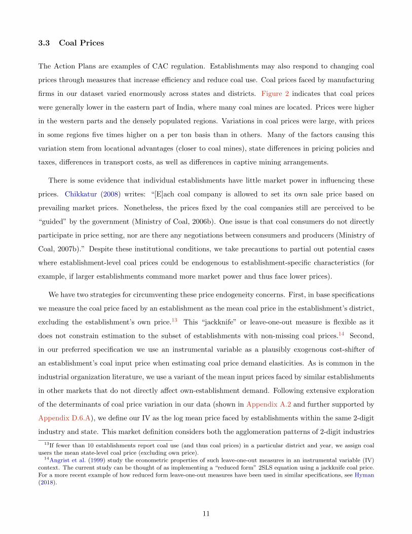
3.3 Coal Prices

The Action Plans are examples of CAC regulation. Establishments may also respond to changing coal

prices through measures that increase efficiency and reduce coal use. Coal prices faced by manufacturing

firms in our dataset varied enormously across states and districts. Figure 2 indicates that coal prices

were generally lower in the eastern part of India, where many coal mines are located. Prices were higher

in the western parts and the densely populated regions. Variations in coal prices were large, with prices

in some regions five times higher on a per ton basis than in others. Many of the factors causing this

variation stem from locational advantages (closer to coal mines), state differences in pricing policies and

taxes, differences in transport costs, as well as differences in captive mining arrangements.

There is some evidence that individual establishments have little market power in influencing these

prices. Chikkatur (2008) writes: “[E]ach coal company is allowed to set its own sale price based on

prevailing market prices. Nonetheless, the prices fixed by the coal companies still are perceived to be

“guided” by the government (Ministry of Coal, 2006b). One issue is that coal consumers do not directly

participate in price setting, nor are there any negotiations between consumers and producers (Ministry of

Coal, 2007b).” Despite these institutional conditions, we take precautions to partial out potential cases

where establishment-level coal prices could be endogenous to establishment-specific characteristics (for

example, if larger establishments command more market power and thus face lower prices).

We have two strategies for circumventing these price endogeneity concerns. First, in base specifications

we measure the coal price faced by an establishment as the mean coal price in the establishment’s district,

excluding the establishment’s own price.13 This “jackknife” or leave-one-out measure is flexible as it

does not constrain estimation to the subset of establishments with non-missing coal prices.14 Second,

in our preferred specification we use an instrumental variable as a plausibly exogenous cost-shifter of

an establishment’s coal input price when estimating coal price demand elasticities. As is common in the

industrial organization literature, we use a variant of the mean input prices faced by similar establishments

in other markets that do not directly affect own-establishment demand. Following extensive exploration

of the determinants of coal price variation in our data (shown in Appendix A.2 and further supported by

Appendix D.6.A), we define our IV as the log mean price faced by establishments within the same 2-digit

industry and state. This market definition considers both the agglomeration patterns of 2-digit industries

13If fewer than 10 establishments report coal use (and thus coal prices) in a particular district and year, we assign coalusers the mean state-level coal price (excluding own price).

14Angrist et al. (1999) study the econometric properties of such leave-one-out measures in an instrumental variable (IV)context. The current study can be thought of as implementing a “reduced form” 2SLS equation using a jackknife coal price.For a more recent example of how reduced form leave-one-out measures have been used in similar specifications, see Hyman(2018).

11

that may generate cost differences due to their distances from coal mines, as well as state-specific decisions

affecting coal use including for example, transportation infrastructure investments.15 We further explore

the identifying assumptions associated with this IV specific in Section 4.

3.4 Air Pollution Data

Although the Action Plans targeted not only air pollution, but also water pollution and land-based toxic

waste, we focus on three measures of air quality – SO2, NO2, and SPM – to compare the impact of Action

Plans with the effects of coal prices on environmental outcomes. SPM, or suspended particulate matter,

captures general air pollution levels. The CPCB website indicates that “RSPM levels exceed prescribed

NAAQS in residential areas of many cities... The reason for high particulate matter levels may be vehicles,

engine gensets, small scale industries, biomass incineration, resuspension of traffic dust, commercial and

domestic use of fuels, etc.”16

SO2 levels are primarily attributable to burning of fossil fuels. In recent years, the the CPCB indicates

that India’s SO2 levels have been declining in major cities, in part because of efforts to introduce cleaner

fuels and new norms for vehicles and fuel quality. There have also been efforts to shift domestic fuel use

away from coal. In our paper, the comparison of Action Plan measures with coal price effects is most

likely to be relevant for SO2 levels, as they are most closely linked to fossil fuel use. NO2 levels are

generally attributable to vehicular exhaust and as such a reduction should be associated with efforts to

reduce pollution associated with vehicle exhaust. The CPCB’s website indicates that “NO2 levels are

within the prescribed National Ambient Air Quality Standards in residential areas of most of the cities.

The reasons for low levels of NO2 may be various measures taken such as banning of old vehicles, better

traffic management etc.”17

Our air pollution data are based on city-level data provided by Greenstone and Hanna (2014) for 2000-

2007. We supplement their data with additional observations from The Energy and Resources Institute

(TERI) in its TERI Energy Data Directory Yearbook (TEDDY) for 2008.18 Figure 1 shows the locations

of air quality monitors. Air quality data are only available for a subset of cities; we mapped each city for

which the data are available to the corresponding district(s) in our dataset. We also show robustness to

using satellite measures of air pollution in Appendix D.3.

15Defining the IV within industry-state-year cells also has the added advantage that coal quality differences across industriesare controlled for.

16Website accessed on June 1, 2015 at http://cpcb.nic.in/Findings.php.17Website accessed on June 1, 2015 at http://cpcb.nic.in/Findings.php.18Results are robust to using the pollutant data from TERI / TEDDY for all years.

12

3.5 Establishment-Level Summary Statistics and Trends

In Table 2, we present summary statistics for the main variables of interest during the baseline period

prior to any SCAP announcement (1998 to 2001), after implementing our preferred sample restrictions

(which includes dropping Delhi throughout the analysis due to a lack of pre-SCAP data).19 Variable

means and standard deviations are broken out by two groups: whether or not an establishment was

ever in a district regulated by an Action Plan (SCAP versus Untreated), along with individual covariate

t-tests comparing baseline means across the two groups. While differences in levels are admissible in our

context, since establishment fixed effects will absorb any time-invariant effects in our DID specifications,

the summary statistics help anchor the magnitude of our estimates, and may be suggestive of potential

threats to identification due to differential pre-trends among the two groups.

Panel A of Table 2 shows that SCAP and untreated districts had similar shares of HPI and HPIxLarge

establishments, where “Large” takes a value of 1 if the establishment had over 100 employees in the first

year it is observed, and zero otherwise.20 While SCAP districts had a slightly lower share of large polluting

establishments, a much higher share of these establishments operated in urban areas (81% versus 50%).

SCAP districts also had a larger number of employees per establishment, and higher revenue output

(but not productivity)—patterns consistent with SCAPs having targeted cities specifically. Notably, the

absence of meaningful differences in entry and exit rates suggests that SCAP regions were not necessarily

targeted based on underlying firm dynamics (insofar as these are captured by entry and exit rates).

Panel B presents analogous statistics for environmental variables. The data show that establishments

in SCAP districts were slightly less likely to have installed pollution abatement equipment (stock) in the

baseline period; more notably, conditional on having equipment, they invested about 1/4 as much as

untreated establishments. SCAP establishments were also less likely to be coal users and, when they do

use coal, consumed less of it. However, establishments in both SCAP and non-SCAP districts faced similar

coal prices across several measures used in the analysis.21 As discussed above, there was large variation in

coal prices across districts, as indicated by the high standard deviations in establishment coal prices. We

further explore the determinants of this variation in Appendix A.2, and display the distribution of our

coal price instrument and endogenous coal prices visually in Appendix A.4. We also report average coal

19As discussed in the next section, while the event years of the analysis run from -5 to +7 (with 0 being the year an SCAPis announced), we restrict many of our specifications to the window from -4 to +6 such that no single policy exerts leverageover the stacked results. This is analogous to imposing a balanced panel requirement for Action Plan-treated districts inevent time. We also drop the Delhi Action plan as our panel currently does not accommodate any data prior to 1998, theyear in which Delhi was mandated to adopt an Action Plan by the Indian Supreme Court.

20This size definition is consistent with other Indian policies which use a size threshold to characterize establishmentheterogeneity.

21These include “own” coal price faced by the establishment, the “jackknife” leave-one-out measure at the district level(discussed above), and the preferred instrumental variable which we further discuss in Appendix A.4.

13

prices by selected 2-digit industries ownership type in Appendix D.6.A, which further highlight industry-

and state-driven sources of variation in coal prices.

We then turn to Figure 3, which shows the underlying data for our main dependent variables of

interest by SCAP status and previews some of our results. Panel A focuses on the subgroup of HPIxLarge

establishments where we detect our main heterogeneous effects, while Panel B shows data collapsed at the

district-year level weighted by district population.22 The top-left plot reveals that while a lower share of

HPI-Large establishments in SCAP districts had pollution control stock prior to SCAP implementation,

SCAP-treated establishments partially closed this gap between 2003 and 2009. The second graph in Panel

A shows that the entry rate of HPI-Large establishments in non-SCAP districts increased post-SCAP;

in contrast, entry in SCAP districts was substantially lower.23 Lastly, the top-right panel shows similar

trends in mean establishment-level TFP before and after SCAP implementation.24

Panel B of Figure 3 shows district-level pollutant trends collapsed by year and SCAP status, weighted

by the population of each district in our sample in 2000. These plots are constructed by aggregating

mean pollutant values in each district-year (averages across all pollution monitors in a given district and

year) by SCAP status, expressed as parts per million (of air volume). Trends in SPM show an increase in

non-targeted districts (commensurate with economic growth rates during the same period), while SPM

levels in SCAP districts remain flat. We observe similar patterns for SO2 and NO2. However, for SO2,

there is a pronounced declining pre-trend in the lead up to the SCAP announcements. In subsequent

regressions (where we consider average and not aggregate pollutant level), we thus also carefully control

for thermal power plant coal use which is not included in our universe of manufacturing establishments,

and we demonstrate that dynamic estimates across event time recover a flat pre-trend (shown in Figure

10).

Taken together, the raw data suggest that the Action Plans had a mild effect on within-establishment

pollution control equipment installation, a reduction in pollutants, little effect on establishment-level

TFP, but a large effect on entry. With the exception of SO2, visual inspection of pre-trends suggests

that the SCAP policies were not necessarily selected on the basis of any observable baseline trend in

dependent variables. However, these means may be masking important unobservable heterogeneity which

could confound both pre- and post-SCAP estimates. In addition to showing stability to a robust Nearest

22Both panels drop Delhi such that the first SCAP announcement occurs in 2002. In Panel A, sampling multipliers areapplied such that means are nationally representative, while Panel B district means are collapsed after expanding samplingweights at the establishment-level.

23Entry equals 1 in the first year an establishment appears in the data, if within three years of the observed ASI “initialproduction year”. We interpret entry effects as SCAPs affecting the targeted group and not the “control” group here, asadditional tests confirm that establishments do not appear to be relocating to non-SCAP regions in response to the policy.See discussion below and Appendix D.4 for further details.

24We also show trends for aggregate output, and aggregate TFP in Figure 12.

14

Neighbor (NN) matching design, in the next section we use historic newspaper references to keywords to

test for anticipation effects, and further validate our research design.

Testing for Anticipation with Historic Times of India References

To explore the extent to which SCAP cities were selected based on preexisting regulatory and pollution

trends, we leverage ProQuest’s Historical Times of India (TOI) newspaper database. The TOI database

contains all English-language articles published in India between 1990 and 2009, and digitizes article

keywords to be searchable at the monthly level. The TOI articles allow us to generate newspaper references

to keywords and specific Indian cities, which we aggregate to the calendar-year and calendar-year-cohort

levels (where cohort refers to cities in each of the three waves of SCAPs). The first 8 lines of each article

are classified as the article’s “abstract”, while the place of publication (first word of each article) is tagged

as the “dateline”. Figure 4 shows two examples of such articles, where keywords are highlighted in green,

dateline in blue, and cities in red. We use these classifications to study trends in two types of keywords:

1. Pollution keywords: pollute, polluting, pollution, pollutant, polluted, emission, so2, sox, sulphur

dioxide, sulphur oxide, no2, nox, nitrogen dioxide, nitrogen oxide, SPM, particulate matter, air

quality, water quality, smog

2. Regulatory keywords: supreme court, action plan, scap, sc, pollution control, cpcb

Our TOI queries count a reference = 1 if a keyword appears anywhere in the article, and the SCAP city

or district is mentioned in the article abstract (including the dateline).25 We explore these trends across

all 17 SCAP cities, and include Delhi in this exercise as our TOI data go back to 1990, providing ample

pre-trend years prior to the 1998 Delhi SCAP.26 Figure 5 shows our results from this exercise. In Panel

A, we restrict attention to the balanced panel corresponding to the year coverage in our ASI analysis

sample, where 0 indicates the year an SCAP is announced. We first residualize annual city references by

calendar year to difference out noise common to all regions, and then mean-collapse by baseline city share

of overall references to account for different city sizes and TOI coverage, resulting in event-year weighted

means.

Panel A shows that references to regulatory or “SCAP” keywords were flat in the run up to the Action

Plan announcements, and dramatically spike with a one to two year lag following the SCAP mandates,

resulting in double the initial press coverage at the peak. Interestingly, references to pollution keywords

25Reference counts are calculated “with replacement” (we do not exclude an article from further queries if it was alreadycounted) to account for cases in which two distinct cities are associated with the same article.

26For Delhi we use the initial city action plan year of 1996 which preceded the first round of Supreme Court Action Plans,which officially began with the Delhi mandate in 1998.

15

trended downward in the run up to the SCAP policies. This runs counter to the concern that SCAPs

may have targeted cities based on growing public concern about pollution in those locations. There is

also no clear evidence of an “Ashenfelter dip” or anticipatory effects just prior to the announcements,

lending credence to the idea that the policies were largely unexpected.

In Panel B of Figure 5, we also examine unstacked cohort trends by wave of SCAP mandate. These

data indicate that TOI coverage cumulatively spiked twice, first around the initial 1996-1998 Delhi plan,

then again for the 2003 cohort of cities mandated to adopt plans. Rather than reflecting a lack of

compliance among the 2002 cohort, the overall number of references are simply very small in those cities

due to a lack of Times of India English-language coverage in the northern part of India where the 2002

cohort was concentrated. To account for this, in Appendix A.3 we normalize references within cohort to

their level the year prior to SCAP announcement, and show that the 2002 cohort exhibits a 50% to 100%

spike in the number of references in the post-period for SCAP and pollution keywords respectively.

All together, these trends suggest that there was very little anticipation of regulation in these specific

cities just prior to SCAP announcements, while references to pollutants were in fact declining in the run

up to the selection of SCAP cities.

4 Identification Strategy

Having shown that SCAP policies were largely unanticipated, our identification strategy exploits the

differential incidence and timing of the Action Plans. The Action Plans were mandated for certain cities

by the Supreme Court, and (with the exception of Delhi) announced in 2002 and 2003 and implemented

shortly thereafter. We compare districts that implemented an Action Plan against those that did not

(including those that would eventually be mandated to enact Action Plans in the 2003 cohort, prior to

2003), and separately examine effects on establishments in HPI versus non-HPI industries.

For our main establishment-level regressions, we use a generalized difference-in-differences (DID)

method where we estimate the following for establishment i in district d in year t:

yidt = β × SCAPdt + λ× CoalPriceidt + αi + ηt + εidt (1)

The variable SCAP is equal to 1 in a district that receives an Action Plan, in any year during and after

the Action Plan is announced, and 0 otherwise. In our baseline specification, the coal price is equal

to the mean district price, excluding own price, and hence varies at the establishment level. Except

16

when noted, our specifications include establishment fixed effects αi (absorbing any time-invariant effects

specific to the establishment and district) as well as accounting year fixed effects ηt. One concern with this

specification is that the SCAPs may affect coal prices themselves, introducing a “bad control” problem.27

For example, if the Action Plans induce adoption of pollution control equipment that requires higher-

quality and thus more expensive grades of coal (unobserved to the econometrician), this could introduce

complicated biases. We show in Appendix A.2 that the Action Plans appear completely unrelated to

establishment coal prices, and further find that point estimates for β are nearly identical when including

and excluding coal prices in subsequent tables.

We also show coefficient estimate plots using a dynamic version of Equation 1 in event time, where ad

is the year an SCAP is announced in district d, and τ denotes the event year relative to the announcement

(normalizing τ = 0 for establishments in districts that are never mandated an Action Plan):

yidt =6∑

τ=−4

βτ × EverSCAPd × 1{t− ad = τ}+ λCoalPriceidt + αi + ηt + εidt (2)

Here, EverSCAPd is an indicator variable for any district that is eventually targeted by an Action Plan.

While full event years span -5 to +7, we restrict our analysis to the window from -4 to +6 such that no

single policy exerts leverage over the stacked results (a balanced panel requirement). We also omit event

year -1 as a reference variable in all dynamic specifications.

As noted above, many of the Action Plans specifically targeted HPI industries. We might expect

effects to differ for HPI and non-HPI establishments simply because the HPI industries have historically

been major polluters, and have been regulated more heavily. In addition, like many other countries,

India tends to focus its environmental regulations on larger establishments; this ability to target is one of

the potential political economy benefits of CAC regulation. Thus, we also examine whether the Action

Plans had differential impacts for large and small establishments. This yields four HPI-size subgroups of

interest, where j indexes the the subgroup:

yidt = δ1 × SCAPdt ×HPIi × Largei + δ2 × SCAPdt ×HPIi ×NotLargei (3)

+ δ3 × SCAPdt ×NotHPIi × Largei + δ4 × SCAPdt ×NotHPIi ×NotLargei

+ λ× CoalPriceidt + αi +∑j

ηjt + εidt

Unlike previous equations, here we interact time fixed effects with the four HPI-size subgroups such that

27The bad control problem is a subtle form of simultaneity bias, formalized in Angrist and Pischke (2008).

17

coefficients capture within-group effects of SCAP policies.28 To avoid the potentially endogenous reaction

of establishment HPI status and size to the Action Plans, we define an establishment as “HPI” if its

primary product was in an HPI industry the first year it is observed, and “large” if it has more than

100 employees in the first year in which is is observed. Thus, the establishment fixed effects absorb the

direct effects of the HPI and establishment size variables. Finally, we also estimate dynamic versions of

Equation 3 analogous to Equation 2 (not shown for conciseness), to produce heterogeneous coefficient

plots over event time.

We begin by examining the impacts of the Action Plans in isolation (without coal prices) on establishment-

level variables. When the outcome variable is the probability that an establishment reports any pollution

control stock (estimated using a perpetual inventory method as described above) or any coal use, we

implement linear probability models where the outcome of interest yidt is a dummy equal to one if the

establishment reports a positive value of pollution control stock (coal use), and zero otherwise. We also

examine effects on the logarithm of pollution control stock, coal use, and coal intensity of output (tons of

coal per unit of real output), which are conditioned on the establishment having a positive value in the

baseline period.

Other variables we consider at the establishment-level include TFP, entry, and exit. The entry variable

takes on a value of 1 in the first year an establishment appears in the data within three years of the observed

initial production date.29 The exit variable takes on a value of 1 in the year an establishment is officially

declared “closed” in the ASI, so long as it remains closed thereafter.30 When we estimate the effects of the

Action Plans and coal prices on the probability of establishment entry and exit using linear probability

models, we alter Equation 1 to exclude establishment fixed effects in order to identify the effect based on

all establishments, not just entrants and exiters. Finally, we conduct similar regressions at the district

level to examine the effects on district-level pollution measures (SPM, SO2, and NO2):

ydt = β × SCAPdt + λ× CoalPricedt + αd + ηt + εdt (4)

In this set of specifications, we also control for coal use by thermal coal power plants, which account

for approximately three-quarters of India’s coal use.31

28This recovers the same point estimates (but different standard errors) as running regressions by each HPIxSize subgroup.29We do not ascribe an entry value of 1 if the factory was left-censored, and chose the threshold value 3 based on the mean

difference between the reported date of initial production and the establishment’s first appearance in the survey data.30This is a conservative definition of exit as any detection of exit will be understated with respect to establishments not

yet officially declared as closed in the ASI.31The ASI establishment-level data, however, unfortunately do not cover electricity units. Consequently, we cannot include

them in our main specifications as we do not observe any of the main variables of the analysis for thermal coal plants.

18

For establishment-level results, we apply ASI-provided sampling multipliers in our analyses. For

district-level results, we first aggregate the establishment-level data to the district level using sampling

multipliers. We then present results in which each district is weighted by either the initial number of

establishments in the district (“InitEstab” in district-level tables) or the population of the district in the

year 2000 prior to SCAP announcements (‘Pop2000” in district-level tables). In all cases, standard errors

are clustered at the district level.

Nearest Neighbor Matching Estimates

Throughout the analysis, we also present an alternative matched-sample strategy in which we use

a nearest-neighbor (NN) matching procedure to pair each SCAP-treated unit in our sample with an

untreated unit, and run our standard DID estimator using this newly matched control group following

closely the algorithm presented in Abadie and Imbens (2002).32 Intuitively, in establishment-level analy-

ses, our matching estimator finds establishments in untreated districts with similar district characteristics

to SCAP districts; however, it requires that establishments be matched exactly within each of the four

HPI x Size subgroups (which vary by establishment). In district-level analyses, we match only on district-

level variables. We discuss the details of this procedure in Appendix B, including a full list of matching

variables with rationale for their inclusion, discussion of overlap and unconfoundedness assumptions, and

balance tests.

Alternative Control Group

As an additional robustness test, in Appendix C.1 we present results for all of our main regressions

using as a control group establishments located in cities that were identified in 2009-2010 as Polluted

Industrial Areas (PIA) but were not targeted for Action Plans in 2002-2003. A research team including

the CPCB, state pollution control boards, and IIT Delhi gave these industrial clusters and areas Com-

prehensive Environmental Pollution Index (CEPI) scores. The list of 88 industrial clusters included areas

with scores that led them to be flagged as critically-polluted areas, as well as those that improved their

scores. The intuition behind this control group is that it represents establishments in cities that would

have been next most likely to be treated at the time that SCAP cities were selected.

Coal Price Instrument

32In regression tables, we use the header “NN” to distinguish this strategy from DID, though a more apt name is “matcheddifference-in-difference estimator” (Heckman et al., 1997).

19

In our preferred specification, we instrument for establishment coal prices in the equations above

using a Hausman (1996) stye cost shifter that plausibly identifies the coal price elasticity of demand from

common supply shocks unrelated to idiosyncratic coal use. We define our IV as the log mean price faced

by firms within the same 2-digit industry and state in a given year. This market definition captures

variation from both the agglomeration patterns of 2-digit industries that generate cost differences due to

distances from coal mines, as well as state-specific policies affecting coal supply such as infrastructure

investments (see Section 3.3 for further discussion).

Like all instrumental variables, our IV must satisfy three main conditions to recover a local average

treatment effect (LATE): relevance, excludability, and monotonicity (Angrist et al., 1996). Toward rel-

evance, we report the first stage F-statistic on the excluded instrument in all 2SLS tables.33 We also

decompose our 2SLS estimate into its “reduced form” (2SLS numerator) and first stage (2SLS denomi-

nator) to show the extent of variation in both endogenous coal prices and our instrument, as well as to

provide some suggestive evidence that the monotonicty assumption is unlikely to be problematic in our

context (shown in Appendix A.4).34

Regarding excludability, the 2SLS identifying assumption for this IV requires that state-industry-year

specific cost shifters are unrelated to other factors directly impacting coal use beyond the price channel.

One potential violation of this assumption would be if coal supply (including the availability of different

grades of coal quality or other fuel substitutes) were endogenously influenced by trends in the underlying

characteristics of establishments within highly specified industries and regions. While we cannot test

this directly, we show in Appendix A.2 that variation in the 3-digit industry Herfindahl-Hirschman Index

(HHI) within a given state has little influence over coal prices when conditioning on average establishment

price (idiosyncratic establishment fixed effects)—consistent with the claim discussed in Section 3.3 that

individual establishments cannot negotiate with coal providers (Chikkatur, 2008). This also suggests that

it is unlikely that a specific industry in a given state could influence for example, highway upgrades for

coal transportation or other cost shifters. Because all regressions are conditioned on establishment fixed

effects, endogeneity here would also need to originate from differential changes in prices, not just levels,

which makes finding a potential violation even more difficult. Due to these potential limitations on the

IV, however, we consistently show results using both the leave-one-out coal measure, as well as our 2SLS

estimate (which are qualitatively similar), and report a range of estimates.

33We report the cluster-robust Kleibergen-Paap statistic (equivalent to Angrist-Pischke test for one endogenous regres-sion), and Cragg-Donaldson joint F-statistic in heterogeneous specifications where the IV is interacted by the four HPI-Sizesubgroups.

34Like excludability, monotonicity cannot be tested explicitly. However, one necessary condition is that compliers with theinstrument should appear to comply in the same direction—in our case, higher coal IV values should always weakly increasewith endogenous coal prices and decrease with coal use.

20

5 Establishment-Level Results

5.1 Pollution Control Equipment

Table 1 showed that pollution control equipment adoption received the most widespread attention in

Action Plan implementation. We begin by testing whether the Action Plans indeed increased the proba-

bility that an establishment reports a positive value for pollution control stock or increased the amount

invested in abatement equipment conditional on having equipment prior to the SCAP announcement. We

refer to these as the extensive and intensive margins respectively. Columns (1) and (4) of Table 3 report

the results from estimating Equation 1 for pollution control stock and log pollution control investment

respectively. These show that in the aggregate the Action Plans had no substantial impact on either

the probability that an establishment had pollution control equipment, nor intensive margin abatement

investments.

When we check for CAC targeting, however, we find evidence that large establishments in HPI indus-

tries were indeed likely to have received additional targeting or scrutiny. Columns (2) and (4) of Table

3, present these estimates using the specification in Equation 3. Column (2) shows that Action Plans

are associated with a mild increase in the probability that large establishments in HPI industries—those

most likely to be targeted by the Action Plans—report any pollution control stock. The coefficient on

the interaction term (SCAP X HPI X Large) of 0.0350 in column (2), suggests that the Action Plans

increased the probability of non-zero abatement investment by about 3.5 percentage points, with standard

errors corresponding to significance at the 5.7% level (a p-value of 0.057). The point estimate remains

unchanged when using PIA districts as a control group (column 1 in Appendix Table C.2). Results are

also similar when using our nearest neighbor matching strategy in column (3). With 3,677 establishments

in the HPI-Large category in column (2), this effect represents 130 large HPI establishments starting to

invest in pollution control equipment.

Turning to intensive margin results in column (5), we find that HPI-Large establishments with pre-

existing abatement equipment in the baseline in fact divest about 17% of their equipment in response to

the Action Plans. One potential explanation for the contrasting findings on pollution control investment

is that regulators may focus on a subset of large HPI establishments, thus allowing backsliding among

non-targeted establishments, including large HPI establishments that already possessed abatement equip-

ment. While data limitations prevent us from tracking specific types of pollution control equipment over

time, additional results (discussed later and shown in Table 7) suggest that effects were concentrated in

regions that were less compliant with previous environmental regulations in the baseline period, consistent

21

with regulators targeting low-hanging fruit. While NN matching estimates in column (6) do not detect

divestment effects, note that the observation count in this regression is much smaller due to subsetting

on the union of being in both the matched control group sample and having abatement equipment in the

baseline period. The PIA control group regressions also fail to detect significant divestment effects (see

Appendix Table C.2). In the latter case the coefficient is still negative, but more than halved relative to

our baseline specification.

To examine the dynamic nature of the effects and assess pre-trends visually, we plot dynamic coeffi-

cient estimates corresponding to columns (2) and (4) using a variation of Equation 2 in Figure 6. Figure

6 first shows that pre-trends in heterogeneous subgroups appear relatively flat prior to the SCAP an-

nouncement year. In the case of extensive margin HPI-Large effects, plants install equipment with a one

year lag (consistent with the SCAP implementation rather than announcement year) and appear to retain

the equipment throughout the post-period. On the intensive margin, establishments instead gradually

divest their equipment over time; dynamics consistent with receiving a sharper signal that they are not

being targeted as more time elapses following the SCAP announcement. In Appendix B.3, we also show

corresponding nearest neighbor dynamic estimates, which exhibit similarly flat pre-trends.

5.2 Exit and Entry

The second largest stated target of the action plans was the use of plant relocations, including directives

issued by the Supreme Court to close specific plants and threaten future closure of noncompliant plants

(see Table 1 and associated institutional details). We test for evidence of such exit in Table 4. Following a

similar analysis structure as before, we present results both overall and by subgroups that were particularly

targeted by the SCAPs, followed by estimating dynamic exit rates over event time in Figure 7.

In Table 4 columns (1) and (3), we find evidence that the SCAPs induced mild exit among estab-

lishments, particularly in non-HPI industries. While the exit rates are small, non-HPI establishments

are numerous, and it is possible that directives targeting their closures (such as relocating small brick

kiln plants as discussed above) occurred in a “one-shot” round of exit. Figure 7 appears to confirm this

interpretation, showing that exit was entirely concentrated in the period 2 years after the SCAPs were

announced (one year after they begun to be implemented). Our definition of exit is conservative: it may

understate true exit rates if establishments are not officially declared to be closed in the ASI (or if this

occurs with a lag). Because we cannot distinguish between whether this exit is a true economic outcome

or instead the result of a noisy measure of exit, we err on the side of caution in our interpretation here.35

35In the dynamic version of the NN estimates in column (4) shown in Appendix B.3, we also see a similar dynamic exit

22

Although the Action Plans were never explicitly about deterring entry, it is one of the margins along

which we see an unambiguously robust result. Column (6) of Table 4 provides evidence that new entry

into SCAP districts was strongly deterred in HPI industries. The point estimates imply that entry into

targeted cities decreased on average by 4.5 percentage points in the post period (on a base of roughly

19,000 total HPI establishments). This corresponds to a 31% decrease over a pre-SCAP baseline entry

rate of 14.37% for HPI establishments. The dynamic effects in the right panel of Figure 7 show that

this entry deterrence gradually increased over time among HPI establishments—possibly linked to an

increase in the perceived likelihood of costly regulation—and were sustained to the end of the sample

period. Note that when analyzing exit and entry, we present NN matching estimates for exit but not

entry, because we have no pre-entry data for establishments. The results are, however, robust to our

PIA control group specification (Appendix Table C.2 column 7) and NN matching done exclusively with

district-level variables (results available upon request).

One natural question that arises when finding effects on entry and exit, is what happens to targeted

establishments that would have remained in, or entered into, SCAP districts absent the intervention.

If large HPI establishments simply escape a targeted city by locating to the fringe of the city, welfare

implications are likely to be negative—the SCAPs distorted private establishment decisions with little

likely impact on decreasing pollutants in highly populous metropolitan areas. Our identification strategy

would also be at risk.

To mitigate this potentially confounding factor, we use a broad geographical range when we define

SCAP cities, including the core city and also surrounding areas, where departing establishments would

ostensibly be most likely to settle. While we cannot track establishments as they move across geographies,

we can evaluate whether entry deterrence in the “core” of the city led to greater entry in the “fringe” of

the city. Toward this end, we classify establishments by whether they operate in core or fringe districts,

and reestimate entry and exit effects within these groupings. The details of this procedure are discussed

in Appendix D.4, which shows that exit and entry rates were nearly identical in the core and fringe, with

no offsetting behavior.

5.3 Coal Use and Comparison with Coal Price Effects

Finally, we check whether there is any evidence that the Action Plans affected fuel use. Since coal is the

dirtiest fuel, we pay particular attention to coal inputs. In Table 5, we show effects of the SCAPs on the

extensive and intensive margins of coal respectively. We find no evidence that the Action Plans changed

pattern. The PIA control group results are also similar.

23

the share of establishments that used coal, but they did significantly reduce the amount of coal consumed

by coal-using establishments. The point estimate in Columns (4) and (7) indicate that the SCAP policies

reduced within-establishment coal use and coal intensity of output by about 14.5% on average—a sizable

magnitude.36 Decomposing effects by HPI-size subgroups reveals that the effects were most concentrated

in large, non-HPI establishments.37 It may be somewhat surprising that the largest percentage changes

are concentrated outside of HPI industries, until we note that some of industries that were not targeted

as HPI are nevertheless quite polluting. Some examples include: textile finishing/dyeing (the largest non-

HPI user of coal inputs), brick making, tyre manufacture, and wood mills. Turning to dynamic effects,

Figure 8 confirms that there are few effects on the extensive margin. The reduction in coal use by large,

non-HPI establishments occurs gradually and persists until the end of our sample period.

From a pollution point of view, a reduction in coal consumption would not be a great success if it led

to a one-to-one substitution towards grid electricity, which runs primarily on coal, or a massive increase

in other cleaner but still polluting fuels, like natural gas. We test for substitution into electricity or other

fuels, with results reported in Appendix D.8. We find no evidence of such substitution. It appears that

targeting dirty fuels through Action Plans led to overall fuel reductions rather than substitution away

from coal to other fuels.

Finally, in Table 6, we compare the effects of the Action Plans with coal price variation on coal use.

In columns (2) and (3), we first estimate a coal price elasticity using the leave-one-out measure discussed

above. We find that a 10% increase in coal prices was associated with about a 5% decrease in coal use

on average. In column (4), we further break up effects by subgroups of interest, which shows that coal

price elasticities are relatively equal across different establishment types (additional evidence that market

power is not affecting price negotiation on average). In columns (5) through (7), we use the cost-shifter

Hausman IV described extensively above, to estimate the effects of coal prices. While the IV elasticity

estimates are larger than the leave-one-out measure, they are within the same degree of magnitude—

implying a coal price elasticity of between -0.5 and -1, close to estimates found for the United States.38

Lastly, we report a strong first stage F-statistic on the excluded IV(s) across all specifications (details in

table notes).

36Using the coefficient -0.157 in column (4), we attain 14.5% from 100 × (exp(−0.157) − 1).37The dependent variable in Table 5 is in logs. When we instead use levels (available upon request), the largest reductions,

which are also strongly statistically-different from zero, come from HPI industries.38Serletis et al. (2010) find an average own-price elasticity of -0.556 for the US using coal price data from 1960-2007, while

the US Energy Information Administration reports regional own-price elasticities ranging from -0.14 to -0.53 (EIA, 2012).

24

Interpreting Magnitudes through a Coal Tax Thought Experiment

The above results suggested that the Action Plans reduced coal use by 12% to 14.5%,39 while a 10%

increase in coal prices is associated with a decline in coal use of between 5% to 10% on average. While coal

taxes did not vary during our sample period, we can compare the magnitude of the Action Plans’ effects

on coal use with what would be required in coal taxes to attain the same reduction, using our average

coal price elasticity. To do this requires two assumptions: (1) First, we assume that the underlying

coal price variation induces the same behavioral response in coal use that would arise increasing the

average coal price through an excise tax (an equal pass-through assumption); (2) Second, we assume that

higher average tax rates affect coal use proportionally across the whole support of baseline prices (an

out-of-sample assumption).

The coefficient on coal price in column (2) of Table 6 (-0.477), suggests that achieving a 12%-14.5%

reduction in coal use would require a coal tax of about 25-30% on average. If we consider the IV re-

sult for coal price in column (5) of Table 6 (-0.863), a 12%-14.5% reduction in coal use would require

a coal tax of about 14-17%. India has placed a variety of different taxes on coal, including royalties,

GST taxes, and a coal cess, which started at Rs. 50 per tonne in 2010 and was subsequently raised

to Rs. 400 per tonne by 2016 (IISD (2017)). Tongia and Gross (2019) estimate a total tax on coal of

about Rs. 859 per ton (in 2016). Considering only the Rs. 400 cess that was added since our sample

period, the current coal tax is about 15% of current nominal prices (using a spot price of 2,653 Rs/tonne

received by Coal India in 2018-2019, as reported by The Economic Times). Thus, the current coal cess

of 15% is on the low end of the range (15-30%) that would have the same effect as the SCAP on coal use.40

Action Plans vs. Prices in a Context of Weak Enforcement

The above exercise demonstrated that while coal taxes are likely to have a broad-based impact on

establishments, they need to be large in magnitude to induce average coal reductions commensurate with

Action Plan regulations. Yet we also showed earlier that Action Plans tend to be applied selectively to

certain types of establishments (especially those that are large and high-polluting to begin with). In this

subsection we explore whether CAC and price effectiveness vary by the degree to which enforcement is

complied with—an important source of variation in emerging markets.

Toward this end, we use baseline state environmental compliance rates prior to SCAP announcements,

reported by State Pollution Control Boards and provided by Greenstone and Hanna (2014), to test for

39Using the coefficient -0.157 in column (1), we obtain 14.5% from 100× (exp(−0.157)− 1). Using the coefficient of -0.128in column (5), we obtain 12% from 100 × (exp(−0.128) − 1).

40Considering the full set of levies on coal, the current tax is on the high end of the range.

25

differential coal price and CAC effects for high and low compliance states separately. The compliance rate

for a given state is calculated as the share of plants flagged as compliers, over a denominator including

compliers, defaulters, and plant closures.41 We then define high and low compliance states relative to the

median compliance rate prior to any SCAP announcement. We report these results in Table 7, using a

variant of Equation 3 that uses compliance-by-year fixed effects in place of HPI-size-year fixed effects to

estimate within high and low com compliance subgroups.

Consistent across all specifications, we find that previously low-compliance states were those in which

the effects of Action Plans were concentrated no matter the dependent variable. Supreme Court man-

dates thus appear to be most effective in places that were previously non-compliant with environmental

regulations, suggesting a scope for CAC targeting to fill in the gaps when regulatory compliance rates are

low in general. In contrast, coal prices do not have larger impacts on coal use in low compliance states.

In fact, the coal price elasticity is lower in low-compliance states.

5.4 TFP Costs

Our findings so far indicate that the Action Plans induced some large polluters to start investing in

abatement equipment, and reduced coal use. We now turn to the cost side, and examine whether these

regulations affected average TFP.42 TFP is an appealing cost measure because it unambiguously captures

true economic costs (such as innovation) net of factor substitution responses to expensive pollution control

equipment installation (which we treat as a variable rather than fixed input). While establishments

may hire workers to operate the newly mandated equipment, or lay off workers to pay for the new

equipment, productivity is a sufficient statistic that captures total establishment costs from moving away

from (privately optimal) pre-regulation factor choices.

Table 8 compares the effects of Action Plans and coal prices on TFP. Columns (1) through (6) show

our preferred Ackerberg et al. (2006) measures with and without effects of coal prices, while columns (7)

through (9) provide a Solow Residual measure of TFP as a benchmark. The results reveal that the Action

Plans had very little effect on establishment productivity. While some specifications detect a negative

effect at the 10% level for HPI-Large establishments—those shown earlier to have adopted pollution

control equipment—the results are generally noisy, and reject the presence of major TFP costs. This lack

of significant TFP costs is further supported by dynamic coefficient plots in Figure 9, which show that the

mild negative effects detected in the table cannot be cleanly identified as visually distinct from noise in

41Results are qualitatively similar when removing closures from the denominator.42Our preferred TFP measures also control for the probability of exit in estimation procedures. However, given evidence

that establishments do not appear to be relocating, we do not focus on aggregate TFP and reallocation issues here.

26

the baseline, and the results using the PIA control group in Appendix Table C.2 which show no economic

or statistically-significant differences. In Appendix D.1.A, we further show qualitatively similar results

using methods from Levinsohn and Petrin (2003) and Olley and Pakes (1996). We also find very mild

negative effects of higher coal prices on TFP, however this is in part expected as TFP is mechanically

calculated using coal among other inputs.

To further hone in on whether the mild TFP effects for HPI-Large establishments are driven by

extensive margin pollution control equipment installations, in Appendix D.1.B we explore the effects

of Action Plans differentially for establishments which had pollution control equipment prior to SCAP

announcements, and those that did not. Focusing on those with no pollution control stock in the baseline,

we see nearly identical estimates to the overall effects, suggesting that indeed the mild negative effects

among HPI-Large establishments may in fact be concentrated among the small share of establishments

that install equipment in response to the policies.

6 Air Quality

So far, we have shown that both the Action Plans and coal prices affected establishment outcomes, albeit

in different ways. In this section we ask whether either this command-and-control regulation or coal prices

had any impact on air quality.

Supreme Court Action Plans could have influenced emissions through a variety of measures mandated

by the plans. The different plans had components targeted at vehicles, which could lead to a relationship

between Action Plan passage and different measures of air pollution, regardless of whether industrial

pollution control measures were implemented effectively. However, other components of these plans

focused on industry, including on high-polluting industries in particular; and our findings show that they

encouraged investment in pollution abatement among large establishments and deterred entry across all

HPI establishments. For these plan components, we would expect Action Plan passage to affect air quality

through changes in emissions.

Table 10 shows the results from district-level regressions in which the outcome variables are ground-

level SPM, SO2 and NO2 concentrations.43 In the footer of each regression model, we list whether the

regression is weighted by baseline district population in the year 2000 (prior to any SCAP announcement),

or the initial number of establishments in the baseline period. The former provides a population-exposed

measure of pollutants conducive to focusing on populous ares, while the latter focuses on industrially-

43See Section 3.4 for a description of district-collapsed pollutant data, and Table 9 for district-level summary statistics.

27

concentrated districts. It bears repeating that there is good coverage of Action Plan districts by pollution

monitors, as was shown in Figure 1.

Starting with SPM in columns (1) through (3) using population-weighted exposure measures, we find

coefficients on the Action Plan variable ranging between -0.089 and -0.171 depending on the specification—

declines of 7.6% to 15.7% in average SPM. While statistical significance is only detected using NN-

matching estimates, Figure 10 shows dynamic plots corresponding to the DID estimates, and indicates

that SPM coefficients are statistically significant at the 5% level in the two event years just after the

SCAPs are implemented—roughly a year after the announcement date—and remain negative throughout

the sample period. Figure 10 also suggests that pre-SCAP trends in SPM are flat, and that the event-study

break in SPM after the SCAP announcement appears distinct from any pre-SCAP noise. We further note

that dynamic DID effects on SPM are very similar when comparing event study plots to our NN strategy

(see Appendix B.3 panel (c)). This is consistent with Greenstone and Hanna (2014), who find similar

coefficients that are not statistically significant.44 In column (4) however, effects are not statistically

significant when weighting by number of initial establishments.

Moving to SO2, we find no evidence of statistically significant declines in SO2 associated with the

Action Plans in populous areas (again consistent with Greenstone and Hanna (2014)), whether controlling

for thermal power plant coal usage or not. This is one result that differs when using satellite data. The

satellite data regressions that are restricted to districts with air quality monitors or districts that contain

PIAs (Appendix Table D.3.2) show evidence of a close to 4% reduction in SO2 levels. Using land-based

monitors, only column (8) indicates a large negative effect on SO2 when considering effects weighted

by industrial concentration. In contrast, coal prices appear to be strongly linked with reduced SO2

pollution. Since SO2 levels are primarily associated with the burning of fossil fuels, the significant and

negative impact of rising coal prices on SO2 emissions is plausible. The negative coefficient, which varies

between -0.119 and -0.204, indicates that a 10 percent rise in coal prices at the district level would be

associated with a reduction in SO2 emissions of between 1 and 2%. Finally, we do not find evidence of

NO2 declines in response to the Action Plans. If anything, NO2 shows an increase in the post-period

when using population-weighted measures.

44For transparency, we replicate the Greenstone and Hanna (2014) results in Appendix D.2 using the timing definition intheir paper in panel (a) (implementation-year) and the timing in our paper in panel (b) (announcement-year).

28

7 Falsification Test

Two central findings from our DID estimation are that more large HPI establishments adopted pollution

control equipment in response to the Action Plans, and that HPI establishments were deterred from

entering Action Plan cities. While our results are robust to a nearest neighbor matching strategy, and

both methods show relatively flat pre-trends in dynamic plots, selection on unobservable characteristics

of Action Plan cities may still remain an identification concern. Although multiple events (i.e. the fact

that the Action Plans were implemented at different times across different cities) aid in identification,

since part of the control group contains establishments that will eventually be treated (with presumably

similar pre-trends around the timing of the Action Plan mandates), our sample restrictions limit this

differential timing to only the 2002 and 2003 SCAP waves. To provide additional evidence that selection

concerns are minimal in our context, we thus implement a non-parametric permutation test following

Chetty et al. (2009), that has been applied in a number of subsequent public finance papers with common

trends identification assumptions.45

The idea in our context, is to run a permutation test that generates placebo estimates from reassigning

treated districts to be treated in every possible year-district combination in our sample, and graphically

inspect where the true estimate falls with respect to the placebo estimate distribution. If we find that the

estimate from our preferred specification is far larger than the majority of placebo estimates, this would

indicate a low p-value on our estimate—i.e. that we are not finding spurious effects due to preexisting

differential trends in years and subsets of districts in which we would not expect to find strong effects.

Were there instead selection on unobservables, then reassigning the timing of treated districts should lead

to a distribution around the “true estimate”, as the econometrician would detect this secular pre-trend

no matter the timing of the policy.

In Figure 11, we present the empirical CDF of placebo estimates from estimating equation Equation

3, plotting the simulated coefficients on SCAP-HPI-Large. As the combinatorial space for all such per-

mutations would be enormous (8 years including 2001 to 2008 raised to 16 possible cities ≈2.8e+14),

in practice, we take 1000 i.i.d. random draws to assign treatment-years to each of the 16 SCAP cities.

We indicate with a red vertical line the true treatment estimate of the effect of SCAP-HPI-Large on the

probability of pollution control use reported in column (2) of Table 3 (0.035), and entry in column (6) of

Table 4 (-0.0462) . Figure 11 confirms that the effect level we find in both cases, far exceeds the large

majority of all other possible permuted placebo effects.

45See for example Chodorow-Reich et al. (2013) for a prominent and influential example of this.

29

8 Concluding Remarks

In this paper, we examined the impact of India’s Supreme Court Action Plans—a major set of CAC

policies—on the behavior of manufacturing firms. Using a comprehensive panel of Indian establishments,

we found that the CAC regulations led to an increase in the number of large establishments in targeted,

highly-polluting industries with pollution control stock, and a decrease in coal consumption among large

establishments in both targeted and non-targeted industries. The Action Plans did not substantially

affect establishment-level TFP, but did have a strong deterrent effect on the entry of establishments in

highly-polluting industries. Examining district-level air quality data, we find that the Action Plans are

associated with a decrease in particular matter that is concentrated in highly populated areas, and with a

decrease in SO2 in industrially-concentrated areas. Comparing the effects of these CAC regulations with

the potential impact of a tax on coal - which we estimate by using the large variation in coal prices - we

find that a 15-30% coal tax would be required in order to achieve the same reduction in coal use as was

achieved by the Action Plans.

One key takeaway from our analyses is that the effects of the CAC regulations were concentrated in

certain industries and areas, whereas the price effects were broadly distributed. The main impacts of the

Action Plans were observed among large establishments, consistent with regulators focusing their enforce-

ment in the most cost-effective way. In addition, the increased investment in pollution control equipment

and the reduction in coal use were largely confined to states where establishments were previously less

compliant - suggesting targeting of non-compliant establishments and areas. In contrast, establishments

of all sizes, and in all areas, responded to coal price increases.

An important concern with environmental regulations are that they can impose substantial costs on

establishments – a concern that is particularly salient in a developing country. We examined the impact of

the Action Plans on TFP, and found small negative impacts at the establishment level. We did, however,

find large deterrent effects - entry for both small and large establishments in highly-polluting industries

in SCAP districts fell following the implementation of the Action Plans.

A key contribution of our study is that we examine both the costs and the benefits of CAC regulations.

We document benefits in the form of additional pollution abatement, reduced coal use, and improved air

quality; as well as potential costs in terms of small declines in establishment-level TFP, as well as large

effects on entry into highly-polluting industries. We show that it does not appear that the entry effects

are simply driven by establishments relocating from the core of a city to the fringe. However, it is not

clear whether the entry deterrence has a negative impact on overall output or employment. A complete

30

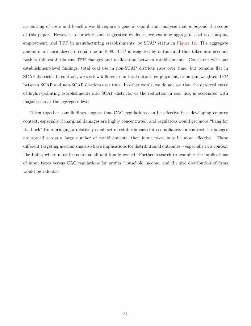
accounting of costs and benefits would require a general equilibrium analysis that is beyond the scope

of this paper. However, to provide some suggestive evidence, we examine aggregate coal use, output,

employment, and TFP in manufacturing establishments, by SCAP status in Figure 12. The aggregate

amounts are normalized to equal one in 1998. TFP is weighted by output and thus takes into account

both within-establishment TFP changes and reallocation between establishments. Consistent with our

establishment-level findings, total coal use in non-SCAP districts rises over time, but remains flat in

SCAP districts. In contrast, we see few differences in total output, employment, or output-weighted TFP

between SCAP and non-SCAP districts over time. In other words, we do not see that the deterred entry

of highly-polluting establishments into SCAP districts, or the reduction in coal use, is associated with

major costs at the aggregate level.

Taken together, our findings suggest that CAC regulations can be effective in a developing country

context, especially if marginal damages are highly concentrated, and regulators would get more “bang for

the buck” from bringing a relatively small set of establishments into compliance. In contrast, if damages

are spread across a large number of establishments, then input taxes may be more effective. These

different targeting mechanisms also have implications for distributional outcomes – especially in a context

like India, where most firms are small and family owned. Further research to examine the implications

of input taxes versus CAC regulations for profits, household income, and the size distribution of firms

would be valuable.

31

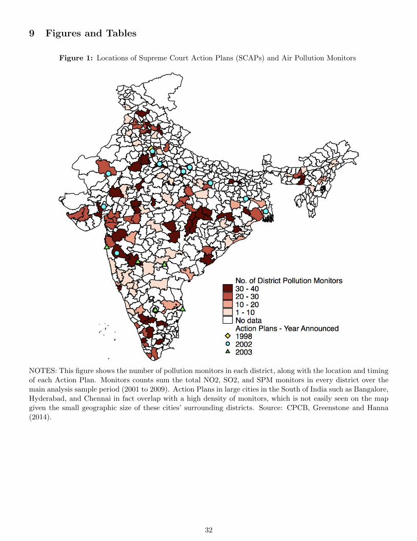
9 Figures and Tables

Figure 1: Locations of Supreme Court Action Plans (SCAPs) and Air Pollution Monitors

NOTES: This figure shows the number of pollution monitors in each district, along with the location and timingof each Action Plan. Monitors counts sum the total NO2, SO2, and SPM monitors in every district over themain analysis sample period (2001 to 2009). Action Plans in large cities in the South of India such as Bangalore,Hyderabad, and Chennai in fact overlap with a high density of monitors, which is not easily seen on the mapgiven the small geographic size of these cities’ surrounding districts. Source: CPCB, Greenstone and Hanna(2014).

32

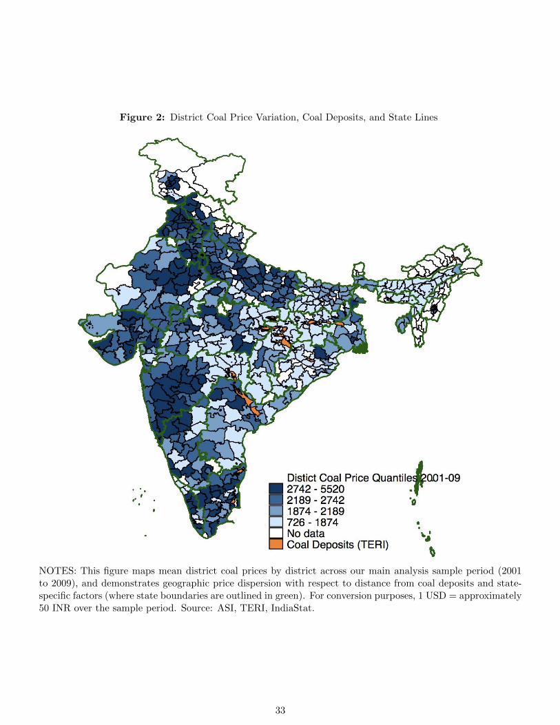
Figure 2: District Coal Price Variation, Coal Deposits, and State Lines

NOTES: This figure maps mean district coal prices by district across our main analysis sample period (2001to 2009), and demonstrates geographic price dispersion with respect to distance from coal deposits and state-specific factors (where state boundaries are outlined in green). For conversion purposes, 1 USD = approximately50 INR over the sample period. Source: ASI, TERI, IndiaStat.

33

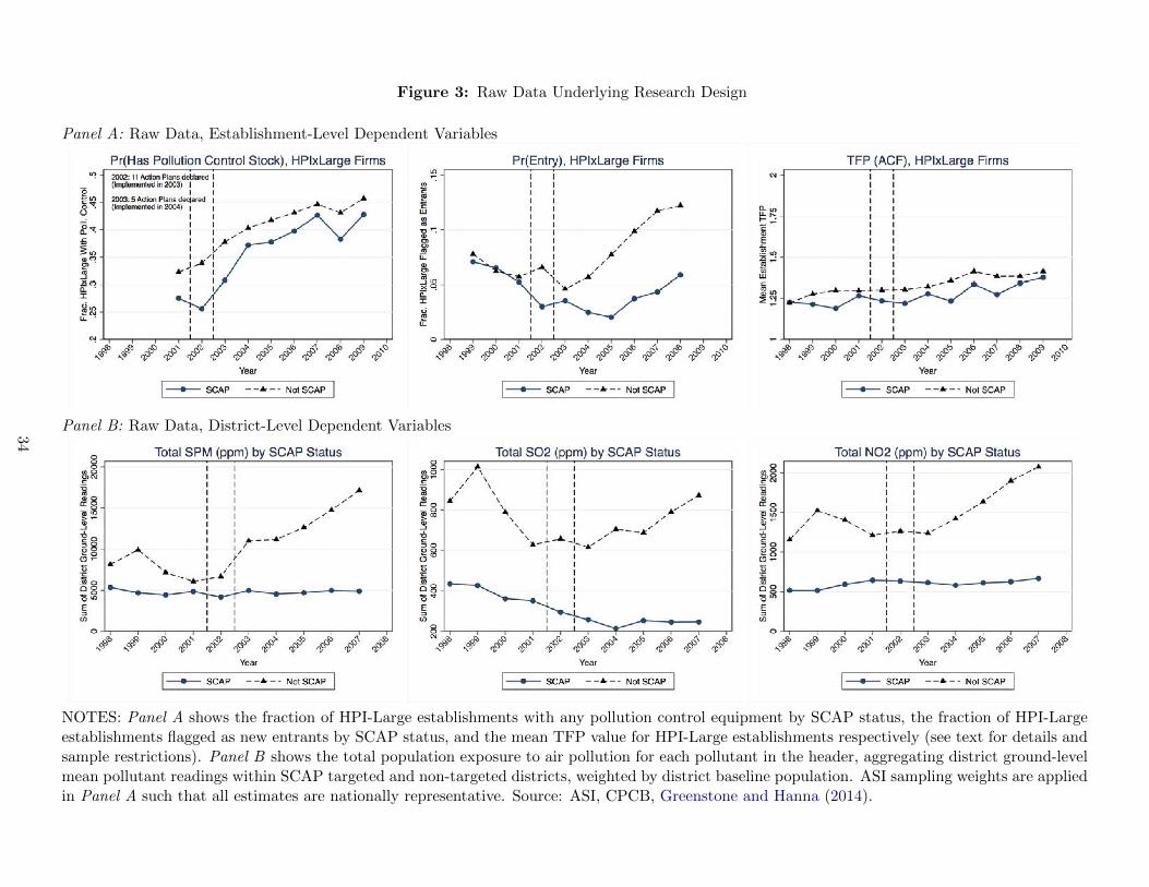
Figure 3: Raw Data Underlying Research Design

Panel A: Raw Data, Establishment-Level Dependent Variables

Panel B: Raw Data, District-Level Dependent Variables

NOTES: Panel A shows the fraction of HPI-Large establishments with any pollution control equipment by SCAP status, the fraction of HPI-Largeestablishments flagged as new entrants by SCAP status, and the mean TFP value for HPI-Large establishments respectively (see text for details andsample restrictions). Panel B shows the total population exposure to air pollution for each pollutant in the header, aggregating district ground-levelmean pollutant readings within SCAP targeted and non-targeted districts, weighted by district baseline population. ASI sampling weights are appliedin Panel A such that all estimates are nationally representative. Source: ASI, CPCB, Greenstone and Hanna (2014).

34

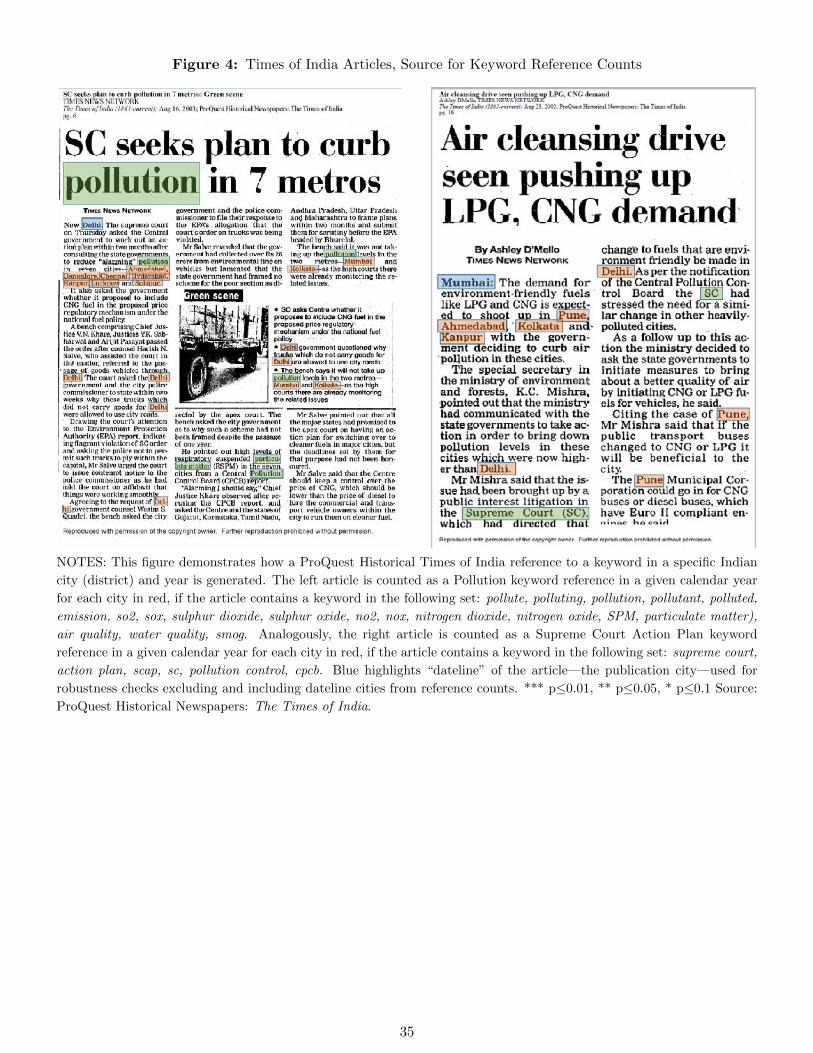
Figure 4: Times of India Articles, Source for Keyword Reference Counts

NOTES: This figure demonstrates how a ProQuest Historical Times of India reference to a keyword in a specific Indian

city (district) and year is generated. The left article is counted as a Pollution keyword reference in a given calendar year

for each city in red, if the article contains a keyword in the following set: pollute, polluting, pollution, pollutant, polluted,

emission, so2, sox, sulphur dioxide, sulphur oxide, no2, nox, nitrogen dioxide, nitrogen oxide, SPM, particulate matter),

air quality, water quality, smog. Analogously, the right article is counted as a Supreme Court Action Plan keyword

reference in a given calendar year for each city in red, if the article contains a keyword in the following set: supreme court,

action plan, scap, sc, pollution control, cpcb. Blue highlights “dateline” of the article—the publication city—used for

robustness checks excluding and including dateline cities from reference counts. *** p≤0.01, ** p≤0.05, * p≤0.1 Source:

ProQuest Historical Newspapers: The Times of India.

35

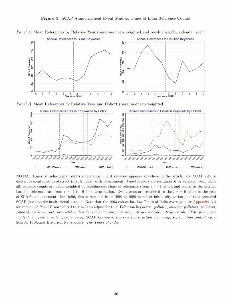
Figure 5: SCAP Announcement Event Studies, Times of India Reference Counts

Panel A. Mean References by Relative Year (baseline-mean weighted and residualized by calendar year)

Panel B. Mean References by Relative Year and Cohort (baseline-mean weighted)

NOTES: Times of India query counts a reference = 1 if keyword appears anywhere in the article, and SCAP city or

district is mentioned in abstract (first 8 lines), with replacement. Panel A plots are residualized by calendar year, while

all reference counts are mean-weighted by baseline city share of references (from τ = -1 to -6), and added to the average

baseline reference rate from τ = -1 to -6 for interpretation. Event years are restricted to the . τ = 0 refers to the year

of SCAP announcement—for Delhi, this is re-coded from 1998 to 1996 to reflect initial city action plan that preceded

SCAP (see text for institutional details). Note that the 2003 cohort has low Times of India coverage—see Appendix A.3

for version of Panel B normalized to τ = -1 to adjust for this. Pollution keywords: pollute, polluting, pollution, pollutant,

polluted, emission, so2, sox, sulphur dioxide, sulphur oxide, no2, nox, nitrogen dioxide, nitrogen oxide, SPM, particulate

matter), air quality, water quality, smog. SCAP keywords: supreme court, action plan, scap, sc, pollution control, cpcb.

Source: ProQuest Historical Newspapers: The Times of India.

36

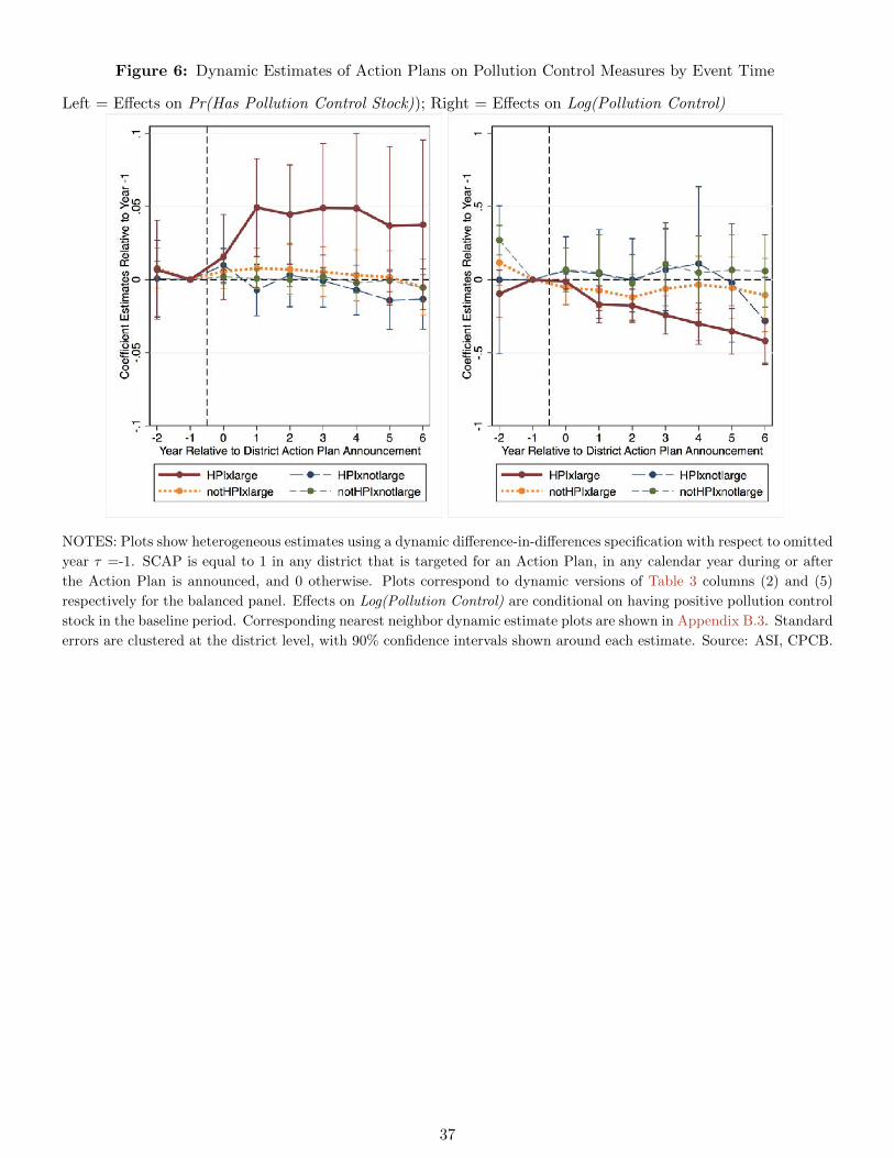
Figure 6: Dynamic Estimates of Action Plans on Pollution Control Measures by Event Time

Left = Effects on Pr(Has Pollution Control Stock)); Right = Effects on Log(Pollution Control)

NOTES: Plots show heterogeneous estimates using a dynamic difference-in-differences specification with respect to omitted

year τ =-1. SCAP is equal to 1 in any district that is targeted for an Action Plan, in any calendar year during or after

the Action Plan is announced, and 0 otherwise. Plots correspond to dynamic versions of Table 3 columns (2) and (5)

respectively for the balanced panel. Effects on Log(Pollution Control) are conditional on having positive pollution control

stock in the baseline period. Corresponding nearest neighbor dynamic estimate plots are shown in Appendix B.3. Standard

errors are clustered at the district level, with 90% confidence intervals shown around each estimate. Source: ASI, CPCB.

37

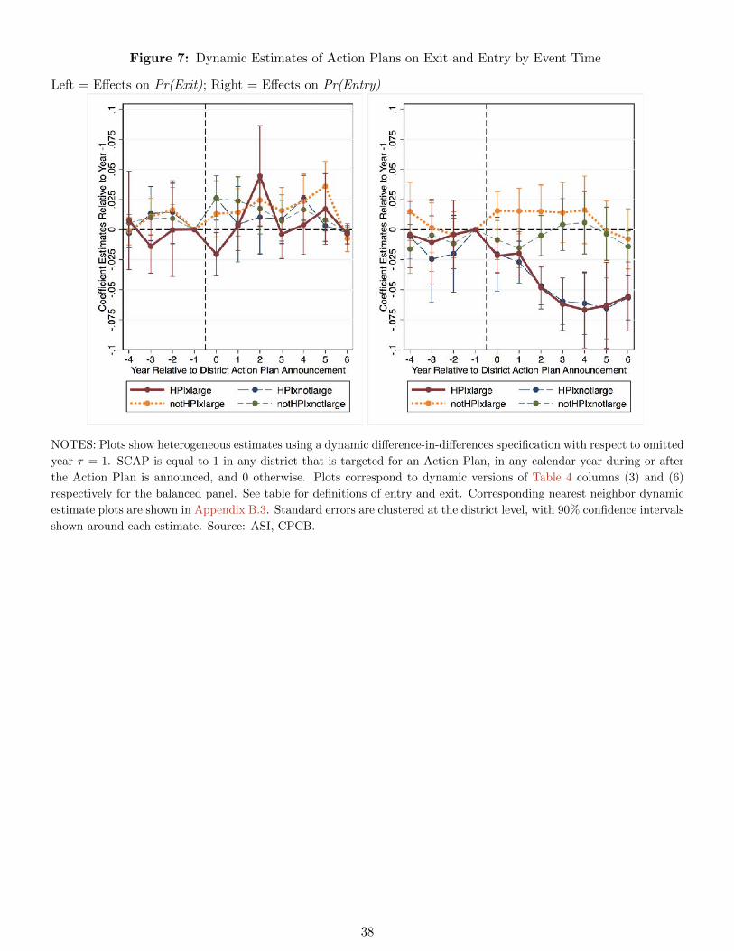
Figure 7: Dynamic Estimates of Action Plans on Exit and Entry by Event Time

Left = Effects on Pr(Exit); Right = Effects on Pr(Entry)

NOTES: Plots show heterogeneous estimates using a dynamic difference-in-differences specification with respect to omitted

year τ =-1. SCAP is equal to 1 in any district that is targeted for an Action Plan, in any calendar year during or after

the Action Plan is announced, and 0 otherwise. Plots correspond to dynamic versions of Table 4 columns (3) and (6)

respectively for the balanced panel. See table for definitions of entry and exit. Corresponding nearest neighbor dynamic

estimate plots are shown in Appendix B.3. Standard errors are clustered at the district level, with 90% confidence intervals

shown around each estimate. Source: ASI, CPCB.

38

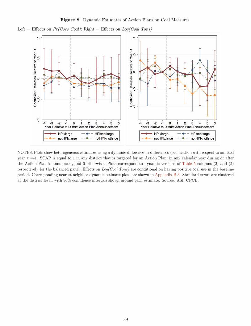
Figure 8: Dynamic Estimates of Action Plans on Coal Measures

Left = Effects on Pr(Uses Coal); Right = Effects on Log(Coal Tons)

NOTES: Plots show heterogeneous estimates using a dynamic difference-in-differences specification with respect to omitted

year τ =-1. SCAP is equal to 1 in any district that is targeted for an Action Plan, in any calendar year during or after

the Action Plan is announced, and 0 otherwise. Plots correspond to dynamic versions of Table 5 columns (2) and (5)

respectively for the balanced panel. Effects on Log(Coal Tons) are conditional on having positive coal use in the baseline

period. Corresponding nearest neighbor dynamic estimate plots are shown in Appendix B.3. Standard errors are clustered

at the district level, with 90% confidence intervals shown around each estimate. Source: ASI, CPCB.

39

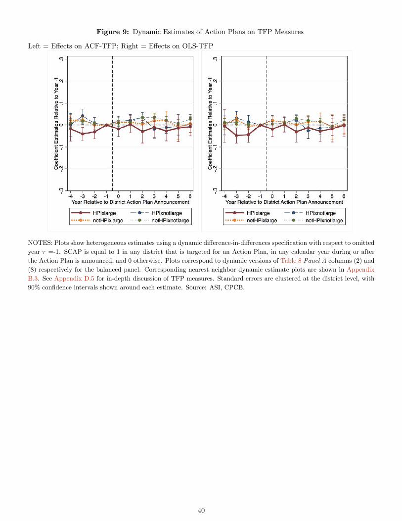
Figure 9: Dynamic Estimates of Action Plans on TFP Measures

Left = Effects on ACF-TFP; Right = Effects on OLS-TFP

NOTES: Plots show heterogeneous estimates using a dynamic difference-in-differences specification with respect to omitted

year τ =-1. SCAP is equal to 1 in any district that is targeted for an Action Plan, in any calendar year during or after

the Action Plan is announced, and 0 otherwise. Plots correspond to dynamic versions of Table 8 Panel A columns (2) and

(8) respectively for the balanced panel. Corresponding nearest neighbor dynamic estimate plots are shown in Appendix

B.3. See Appendix D.5 for in-depth discussion of TFP measures. Standard errors are clustered at the district level, with

90% confidence intervals shown around each estimate. Source: ASI, CPCB.

40

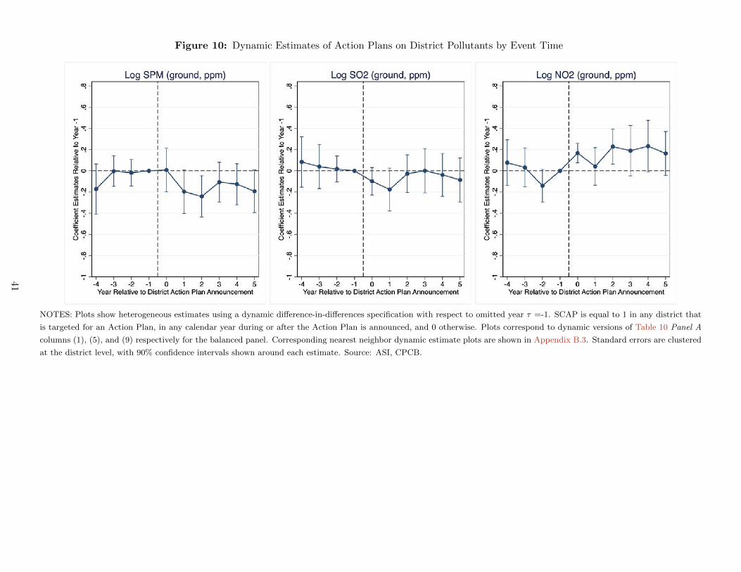
Figure 10: Dynamic Estimates of Action Plans on District Pollutants by Event Time

NOTES: Plots show heterogeneous estimates using a dynamic difference-in-differences specification with respect to omitted year τ =-1. SCAP is equal to 1 in any district that

is targeted for an Action Plan, in any calendar year during or after the Action Plan is announced, and 0 otherwise. Plots correspond to dynamic versions of Table 10 Panel A

columns (1), (5), and (9) respectively for the balanced panel. Corresponding nearest neighbor dynamic estimate plots are shown in Appendix B.3. Standard errors are clustered

at the district level, with 90% confidence intervals shown around each estimate. Source: ASI, CPCB.

41

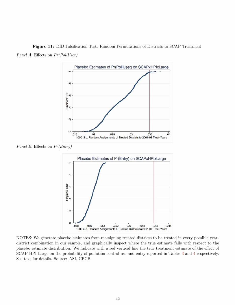
Figure 11: DID Falsification Test: Random Permutations of Districts to SCAP Treatment

Panel A. Effects on Pr(PollUser)

Panel B. Effects on Pr(Entry)

NOTES: We generate placebo estimates from reassigning treated districts to be treated in every possible year-district combination in our sample, and graphically inspect where the true estimate falls with respect to theplacebo estimate distribution. We indicate with a red vertical line the true treatment estimate of the effect ofSCAP-HPI-Large on the probability of pollution control use and entry reported in Tables 3 and 4 respectively.See text for details. Source: ASI, CPCB

42

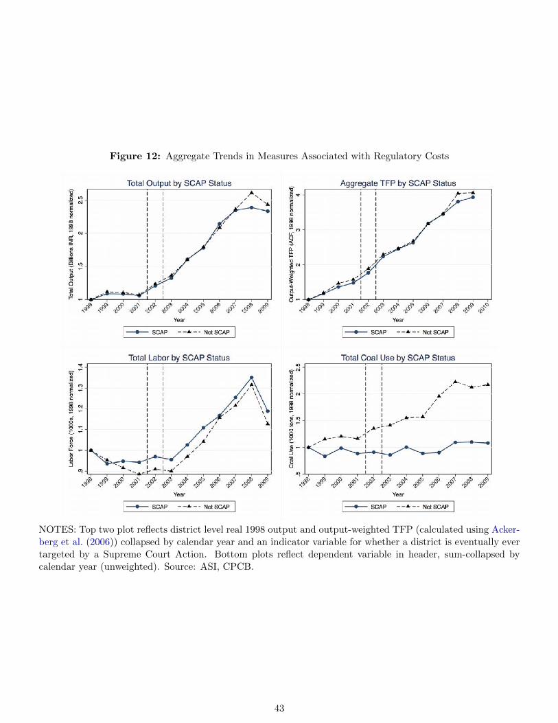
Figure 12: Aggregate Trends in Measures Associated with Regulatory Costs

NOTES: Top two plot reflects district level real 1998 output and output-weighted TFP (calculated using Acker-berg et al. (2006)) collapsed by calendar year and an indicator variable for whether a district is eventually evertargeted by a Supreme Court Action. Bottom plots reflect dependent variable in header, sum-collapsed bycalendar year (unweighted). Source: ASI, CPCB.

43

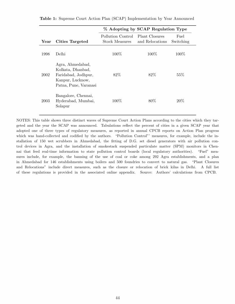
Table 1: Supreme Court Action Plan (SCAP) Implementation by Year Announced

% Adopting by SCAP Regulation Type

Pollution Control Plant Closures FuelYear Cities Targeted Stock Measures and Relocations Switching

1998 Delhi 100% 100% 100%

2002

Agra, Ahmedabad,Kolkata, Dhanbad,Faridabad, Jodhpur,Kanpur, Lucknow,Patna, Pune, Varanasi

82% 82% 55%

2003Bangalore, Chennai,Hyderabad, Mumbai,Solapur

100% 80% 20%

NOTES: This table shows three distinct waves of Supreme Court Action Plans according to the cities which they tar-

geted and the year the SCAP was announced. Tabulations reflect the percent of cities in a given SCAP year that

adopted one of three types of regulatory measures, as reported in annual CPCB reports on Action Plan progress

which was hand-collected and codified by the authors. “Pollution Control”’ measures, for example, include the in-

stallation of 150 wet scrubbers in Ahmedabad, the fitting of D.G. set diesel generators with air pollution con-

trol devices in Agra, and the installation of smokestack suspended particulate matter (SPM) monitors in Chen-

nai that feed real-time information to state pollution control boards (local regulatory authorities). “Fuel” mea-

sures include, for example, the banning of the use of coal or coke among 292 Agra establishments, and a plan

in Ahmedabad for 146 establishments using boilers and 500 foundries to convert to natural gas. “Plant Closures

and Relocations” include direct measures, such as the closure or relocation of brick kilns in Delhi. A full list

of these regulations is provided in the associated online appendix. Source: Authors’ calculations from CPCB.

44

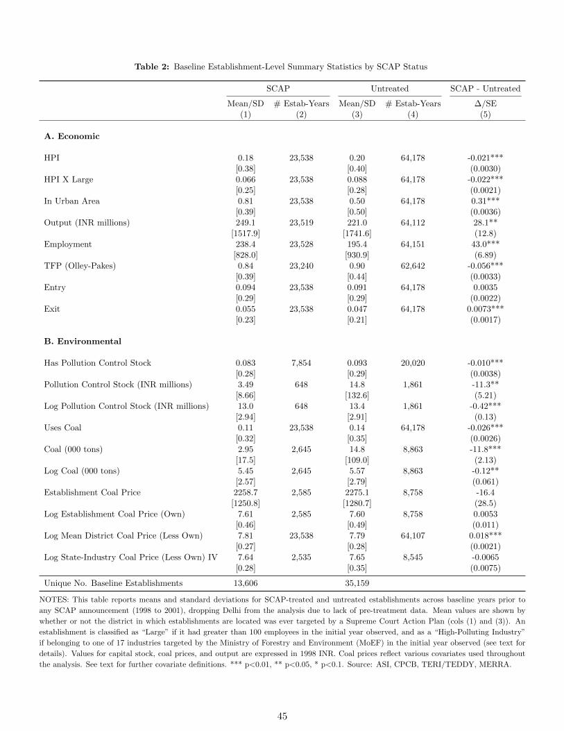
Table 2: Baseline Establishment-Level Summary Statistics by SCAP Status

SCAP Untreated SCAP - Untreated

Mean/SD # Estab-Years Mean/SD # Estab-Years ∆/SE(1) (2) (3) (4) (5)

A. Economic

HPI 0.18 23,538 0.20 64,178 -0.021***[0.38] [0.40] (0.0030)

HPI X Large 0.066 23,538 0.088 64,178 -0.022***[0.25] [0.28] (0.0021)

In Urban Area 0.81 23,538 0.50 64,178 0.31***[0.39] [0.50] (0.0036)

Output (INR millions) 249.1 23,519 221.0 64,112 28.1**[1517.9] [1741.6] (12.8)

Employment 238.4 23,528 195.4 64,151 43.0***[828.0] [930.9] (6.89)

TFP (Olley-Pakes) 0.84 23,240 0.90 62,642 -0.056***[0.39] [0.44] (0.0033)

Entry 0.094 23,538 0.091 64,178 0.0035[0.29] [0.29] (0.0022)

Exit 0.055 23,538 0.047 64,178 0.0073***[0.23] [0.21] (0.0017)

B. Environmental

Has Pollution Control Stock 0.083 7,854 0.093 20,020 -0.010***[0.28] [0.29] (0.0038)

Pollution Control Stock (INR millions) 3.49 648 14.8 1,861 -11.3**[8.66] [132.6] (5.21)

Log Pollution Control Stock (INR millions) 13.0 648 13.4 1,861 -0.42***[2.94] [2.91] (0.13)

Uses Coal 0.11 23,538 0.14 64,178 -0.026***[0.32] [0.35] (0.0026)

Coal (000 tons) 2.95 2,645 14.8 8,863 -11.8***[17.5] [109.0] (2.13)

Log Coal (000 tons) 5.45 2,645 5.57 8,863 -0.12**[2.57] [2.79] (0.061)

Establishment Coal Price 2258.7 2,585 2275.1 8,758 -16.4[1250.8] [1280.7] (28.5)

Log Establishment Coal Price (Own) 7.61 2,585 7.60 8,758 0.0053[0.46] [0.49] (0.011)

Log Mean District Coal Price (Less Own) 7.81 23,538 7.79 64,107 0.018***[0.27] [0.28] (0.0021)

Log State-Industry Coal Price (Less Own) IV 7.64 2,535 7.65 8,545 -0.0065[0.28] [0.35] (0.0075)

Unique No. Baseline Establishments 13,606 35,159

NOTES: This table reports means and standard deviations for SCAP-treated and untreated establishments across baseline years prior to

any SCAP announcement (1998 to 2001), dropping Delhi from the analysis due to lack of pre-treatment data. Mean values are shown by

whether or not the district in which establishments are located was ever targeted by a Supreme Court Action Plan (cols (1) and (3)). An

establishment is classified as “Large” if it had greater than 100 employees in the initial year observed, and as a “High-Polluting Industry”

if belonging to one of 17 industries targeted by the Ministry of Forestry and Environment (MoEF) in the initial year observed (see text for

details). Values for capital stock, coal prices, and output are expressed in 1998 INR. Coal prices reflect various covariates used throughout

the analysis. See text for further covariate definitions. *** p<0.01, ** p<0.05, * p<0.1. Source: ASI, CPCB, TERI/TEDDY, MERRA.

45

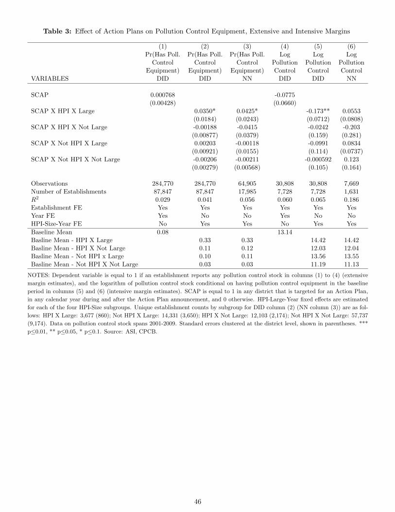
Table 3: Effect of Action Plans on Pollution Control Equipment, Extensive and Intensive Margins

(1) (2) (3) (4) (5) (6)Pr(Has Poll. Pr(Has Poll. Pr(Has Poll. Log Log Log

Control Control Control Pollution Pollution PollutionEquipment) Equipment) Equipment) Control Control Control

VARIABLES DID DID NN DID DID NN

SCAP 0.000768 -0.0775(0.00428) (0.0660)

SCAP X HPI X Large 0.0350* 0.0425* -0.173** 0.0553(0.0184) (0.0243) (0.0712) (0.0808)

SCAP X HPI X Not Large -0.00188 -0.0415 -0.0242 -0.203(0.00877) (0.0379) (0.159) (0.281)

SCAP X Not HPI X Large 0.00203 -0.00118 -0.0991 0.0834(0.00921) (0.0155) (0.114) (0.0737)

SCAP X Not HPI X Not Large -0.00206 -0.00211 -0.000592 0.123(0.00279) (0.00568) (0.105) (0.164)

Observations 284,770 284,770 64,905 30,808 30,808 7,669Number of Establishments 87,847 87,847 17,985 7,728 7,728 1,631R2 0.029 0.041 0.056 0.060 0.065 0.186Establishment FE Yes Yes Yes Yes Yes YesYear FE Yes No No Yes No NoHPI-Size-Year FE No Yes Yes No Yes Yes

Baseline Mean 0.08 13.14Basline Mean - HPI X Large 0.33 0.33 14.42 14.42Basline Mean - HPI X Not Large 0.11 0.12 12.03 12.04Basline Mean - Not HPI x Large 0.10 0.11 13.56 13.55Basline Mean - Not HPI X Not Large 0.03 0.03 11.19 11.13

NOTES: Dependent variable is equal to 1 if an establishment reports any pollution control stock in columns (1) to (4) (extensive

margin estimates), and the logarithm of pollution control stock conditional on having pollution control equipment in the baseline

period in columns (5) and (6) (intensive margin estimates). SCAP is equal to 1 in any district that is targeted for an Action Plan,

in any calendar year during and after the Action Plan announcement, and 0 otherwise. HPI-Large-Year fixed effects are estimated

for each of the four HPI-Size subgroups. Unique establishment counts by subgroup for DID column (2) (NN column (3)) are as fol-

lows: HPI X Large: 3,677 (860); Not HPI X Large: 14,331 (3,650); HPI X Not Large: 12,103 (2,174); Not HPI X Not Large: 57,737

(9,174). Data on pollution control stock spans 2001-2009. Standard errors clustered at the district level, shown in parentheses. ***

p≤0.01, ** p≤0.05, * p≤0.1. Source: ASI, CPCB.

46

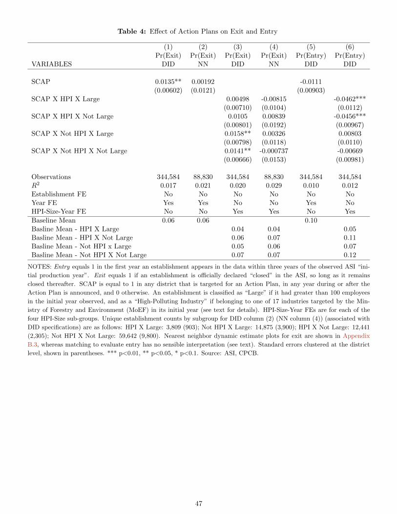
Table 4: Effect of Action Plans on Exit and Entry

(1) (2) (3) (4) (5) (6)Pr(Exit) Pr(Exit) Pr(Exit) Pr(Exit) Pr(Entry) Pr(Entry)

VARIABLES DID NN DID NN DID DID

SCAP 0.0135** 0.00192 -0.0111(0.00602) (0.0121) (0.00903)

SCAP X HPI X Large 0.00498 -0.00815 -0.0462***(0.00710) (0.0104) (0.0112)

SCAP X HPI X Not Large 0.0105 0.00839 -0.0456***(0.00801) (0.0192) (0.00967)

SCAP X Not HPI X Large 0.0158** 0.00326 0.00803(0.00798) (0.0118) (0.0110)

SCAP X Not HPI X Not Large 0.0141** -0.000737 -0.00669(0.00666) (0.0153) (0.00981)

Observations 344,584 88,830 344,584 88,830 344,584 344,584R2 0.017 0.021 0.020 0.029 0.010 0.012Establishment FE No No No No No NoYear FE Yes Yes No No Yes NoHPI-Size-Year FE No No Yes Yes No Yes

Baseline Mean 0.06 0.06 0.10Basline Mean - HPI X Large 0.04 0.04 0.05Basline Mean - HPI X Not Large 0.06 0.07 0.11Basline Mean - Not HPI x Large 0.05 0.06 0.07Basline Mean - Not HPI X Not Large 0.07 0.07 0.12

NOTES: Entry equals 1 in the first year an establishment appears in the data within three years of the observed ASI “ini-

tial production year”. Exit equals 1 if an establishment is officially declared “closed” in the ASI, so long as it remains

closed thereafter. SCAP is equal to 1 in any district that is targeted for an Action Plan, in any year during or after the

Action Plan is announced, and 0 otherwise. An establishment is classified as “Large” if it had greater than 100 employees

in the initial year observed, and as a “High-Polluting Industry” if belonging to one of 17 industries targeted by the Min-

istry of Forestry and Environment (MoEF) in its initial year (see text for details). HPI-Size-Year FEs are for each of the

four HPI-Size sub-groups. Unique establishment counts by subgroup for DID column (2) (NN column (4)) (associated with

DID specifications) are as follows: HPI X Large: 3,809 (903); Not HPI X Large: 14,875 (3,900); HPI X Not Large: 12,441

(2,305); Not HPI X Not Large: 59,642 (9,800). Nearest neighbor dynamic estimate plots for exit are shown in Appendix

B.3, whereas matching to evaluate entry has no sensible interpretation (see text). Standard errors clustered at the district

level, shown in parentheses. *** p<0.01, ** p<0.05, * p<0.1. Source: ASI, CPCB.

47

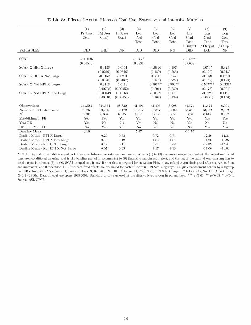
Table 5: Effect of Action Plans on Coal Use, Extensive and Intensive Margins

(1) (2) (3) (4) (5) (6) (7) (8) (9)Pr(Uses Pr(Uses Pr(Uses Log Log Log Log Log LogCoal) Coal) Coal) Coal Coal Coal Coal Coal Coal

Tons Tons Tons Tons Tons Tons/ Output / Output / Output

VARIABLES DID DID NN DID DID NN DID DID NN

SCAP -0.00436 -0.157* -0.153**(0.00573) (0.0831) (0.0689)

SCAP X HPI X Large -0.0126 -0.0161 -0.0896 0.197 0.0567 0.328(0.0219) (0.0346) (0.159) (0.263) (0.120) (0.218)

SCAP X HPI X Not Large -0.0162 -0.0201 0.0805 0.247 -0.0131 0.0620(0.0170) (0.0187) (0.144) (0.227) (0.148) (0.198)

SCAP X Not HPI X Large -0.0116 -0.0119 -0.590*** -0.509** -0.527*** -0.422**(0.00708) (0.00952) (0.201) (0.250) (0.173) (0.204)

SCAP X Not HPI X Not Large 0.000449 0.00163 -0.0789 0.0613 -0.0720 0.0191(0.00440) (0.00651) (0.107) (0.139) (0.0771) (0.150)

Observations 344,584 344,584 88,830 41,596 41,596 8,908 41,574 41,574 8,904Number of Establishments 90,766 90,766 19,172 13,347 13,347 2,502 13,342 13,342 2,502R2 0.001 0.002 0.005 0.011 0.018 0.054 0.007 0.012 0.037Establishment FE Yes Yes Yes Yes Yes Yes Yes Yes YesYear FE Yes No No Yes No No Yes No NoHPI-Size-Year FE No Yes Yes No Yes Yes No Yes Yes

Baseline Mean 0.10 5.47 -11.75Basline Mean - HPI X Large 0.20 0.33 6.72 6.74 -12.36 -12.34Basline Mean - HPI X Not Large 0.15 0.12 4.85 4.84 -11.26 -11.27Basline Mean - Not HPI x Large 0.12 0.11 6.51 6.52 -12.39 -12.40Basline Mean - Not HPI X Not Large 0.07 0.03 4.17 4.18 -11.06 -11.04

NOTES: Dependent variable is equal to 1 if an establishment reports any coal use in columns (1) to (3) (extensive margin estimates), the logarithm of coal

tons used conditional on using coal in the baseline period in columns (4) to (6) (intensive margin estimates), and the log of the ratio of coal consumption to

total output in columns (7) to (9). SCAP is equal to 1 in any district that is targeted for an Action Plan, in any calendar year during and after the Action Plan

announcement, and 0 otherwise. HPI-Size-Year fixed effects are estimated for each of the four HPI-Size subgroups. Unique establishment counts by subgroup

for DID column (2) (NN column (3)) are as follows: 3,809 (903); Not HPI X Large: 14,875 (3,900); HPI X Not Large: 12,441 (2,305); Not HPI X Not Large:

59,642 (9,800). Data on coal use spans 1998-2009. Standard errors clustered at the district level, shown in parentheses. *** p≤0.01, ** p≤0.05, * p≤0.1.

Source: ASI, CPCB.

48

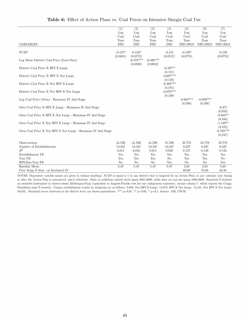
Table 6: Effect of Action Plans vs. Coal Prices on Intensive Margin Coal Use

(1) (2) (3) (4) (5) (6) (7)Log Log Log Log Log Log LogCoal Coal Coal Coal Coal Coal CoalTons Tons Tons Tons Tons Tons Tons

VARIABLES DID DID DID DID DID/2SLS DID/2SLS DID/2SLS

SCAP -0.157* -0.134* -0.121 -0.128* -0.120(0.0831) (0.0773) (0.0747) (0.0778) (0.0770)

Log Mean District Coal Price (Less Own) -0.478*** -0.490***(0.0928) (0.0952)

District Coal Price X HPI X Large -0.437**(0.181)

District Coal Price X HPI X Not Large -0.607***(0.128)

District Coal Price X Not HPI X Large -0.469***(0.181)

District Coal Price X Not HPI X Not Large -0.379***(0.120)

Log Coal Price (Own) - Hausman IV 2nd Stage -0.863*** -0.899***(0.208) (0.206)

Own Coal Price X HPI X Large - Hausman IV 2nd Stage -0.377(0.858)

Own Coal Price X HPI X Not Large - Hausman IV 2nd Stage -0.949**(0.456)

Own Coal Price X Not HPI X Large - Hausman IV 2nd Stage -1.149**(0.525)

Own Coal Price X Not HPI X Not Large - Hausman IV 2nd Stage -0.788***(0.247)

Observations 41,596 41,596 41,596 41,596 35,778 35,778 35,778Number of Establishments 13,347 13,347 13,347 13,347 9,237 9,237 9,237R2 0.011 0.016 0.015 0.020 0.127 0.126 0.123Establishment FE Yes Yes Yes Yes Yes Yes YesYear FE Yes Yes Yes No Yes Yes NoHPI-Size-Year FE No No No Yes No No Yes

Baseline Mean 5.47 5.47 5.47 5.47 5.65 5.65 5.65First Stage F-Stat. on Excluded IV 69.69 70.86 42.35

NOTES: Dependent variable names are given in column headings. SCAP is equal to 1 in any district that is targeted for an Action Plan, in any calendar year during

or after the Action Plan is announced, and 0 otherwise. Data on pollution control stock spans 2001-2009, while data on coal use spans 1998-2009. Reported F-statistic

on excluded instrument is cluster-robsut Kleibergen-Paap (equivalent to Angrist-Pischke test for one endogenous regressor), except column 7, which reports the Cragg-

Donaldson joint F-statistic. Unique establishment counts by subgroup are as follows: 3,809; Not HPI X Large: 14,875; HPI X Not Large: 12,441; Not HPI X Not Large:

59,642.. Standard errors clustered at the district level, are shown parentheses. *** p<0.01, ** p<0.05, * p<0.1. Source: ASI, CPCB.

49

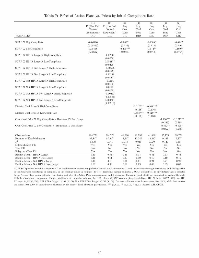
Table 7: Effect of Action Plans vs. Prices by Initial Compliance Rate

(1) (2) (3) (4) (5) (6) (7)Pr(Has Poll. Pr(Has Poll. Log Log Log Log Log

Control Control Coal Coal Coal Coal CoalEquipment) Equipment) Tons Tons Tons Tons Tons

VARIABLES DID DID DID DID DID DID DID

SCAP X HighCompRate -0.00400 -0.00631 0.00696 -0.0447(0.00469) (0.123) (0.125) (0.146)

SCAP X LowCompRate 0.00418 -0.200*** -0.172** -0.169**(0.00607) (0.0765) (0.0706) (0.0758)

SCAP X HPI X Large X HighCompRate 0.00996(0.0256)

SCAP X HPI X Large X LowCompRate 0.0521**(0.0225)

SCAP X HPI X Not Large X HighCompRate -0.00528(0.0125)

SCAP X HPI X Not Large X LowCompRate 0.00134(0.0117)

SCAP X Not HPI X Large X HighCompRate -0.0121(0.0102)

SCAP X Not HPI X Large X LowCompRate 0.0128(0.0130)

SCAP X Not HPI X Not Large X HighCompRate -0.00463(0.00584)

SCAP X Not HPI X Not Large X LowCompRate 0.000501(0.00316)

District Coal Price X HighCompRate -0.517*** -0.518***(0.138) (0.136)

District Coal Price X LowCompRate -0.458*** -0.428***(0.106) (0.108)

Own Coal Price X HighCompRate - Hausman IV 2nd Stage -1.130*** -1.127***(0.289) (0.288)

Own Coal Price X LowCompRate - Hausman IV 2nd Stage -0.557** -0.465*(0.257) (0.268)

Observations 284,770 284,770 41,596 41,596 41,596 35,778 35,778Number of Establishments 87,847 87,847 13,347 13,347 13,347 9,237 9,237R2 0.029 0.041 0.015 0.019 0.020 0.120 0.117Establishment FE Yes Yes Yes Yes Yes Yes YesYear FE No No No No No No NoSubgroup-Year FE Yes Yes Yes Yes Yes Yes Yes

Basline Mean - HPI X Large 0.33 0.33 0.33 0.33 0.33 0.33 0.33Basline Mean - HPI X Not Large 0.11 0.11 0.19 0.19 0.19 0.19 0.19Basline Mean - Not HPI x Large 0.10 0.10 0.21 0.21 0.21 0.21 0.21Basline Mean - Not HPI X Not Large 0.03 0.03 0.09 0.09 0.09 0.09 0.09

NOTES: Dependent variable is equal to 1 if an establishment reports any pollution control stock in columns (1) and (2) (extensive margin estimates), and the logarithm

of coal tons used conditional on using coal in the baseline period in columns (3) to (7) (intensive margin estimates). SCAP is equal to 1 in any district that is targeted

for an Action Plan, in any calendar year during and after the Action Plan announcement, and 0 otherwise. Subgroup fixed effects are estimated for each of the eight

HPI-Size-Compliance subgroups. Unique establishment counts by subgroup for DID column (2) (NN column (3)) are as follows: HPI X Large: 3,677 (860); Not HPI

X Large: 14,331 (3,650); HPI X Not Large: 12,103 (2,174); Not HPI X Not Large: 57,737 (9,174). Data on pollution control stock spans 2001-2009, while data on coal

use spans 1998-2009. Standard errors clustered at the district level, shown in parentheses. *** p≤0.01, ** p≤0.05, * p≤0.1. Source: ASI, CPCB.

50

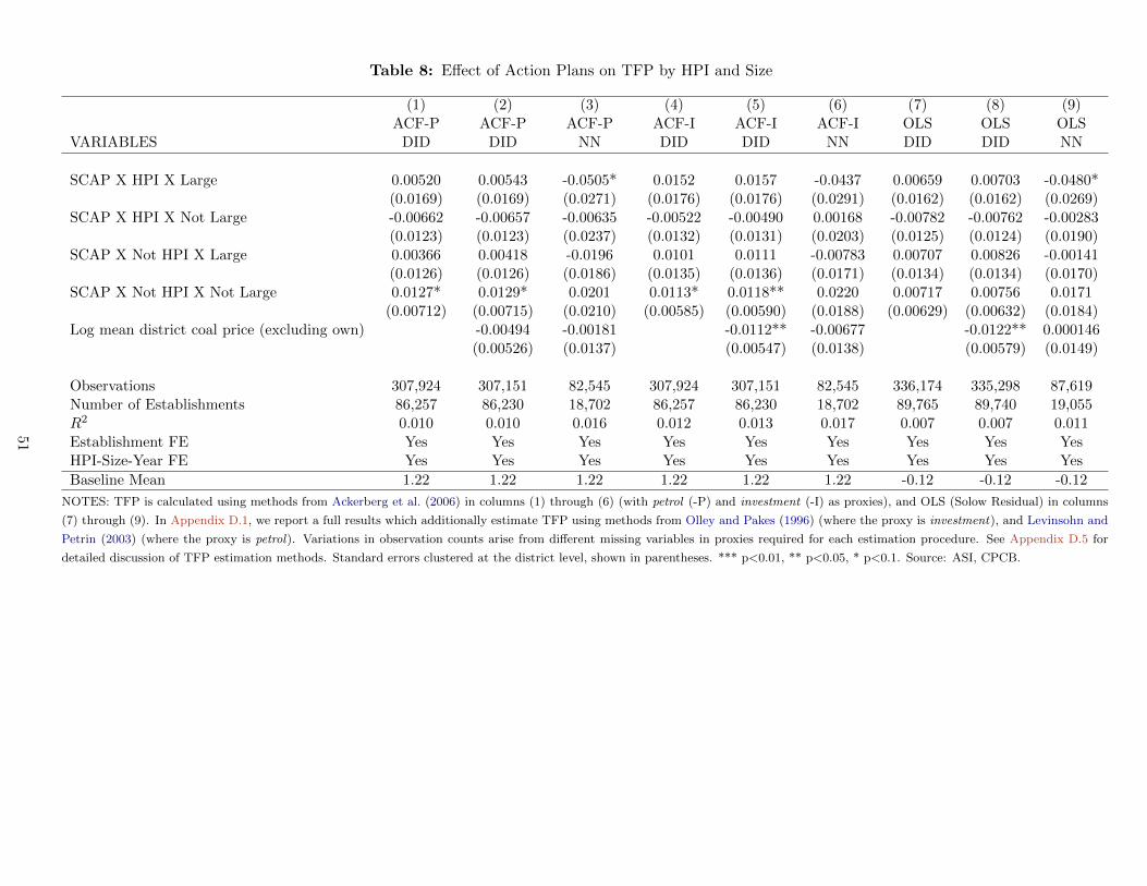
Table 8: Effect of Action Plans on TFP by HPI and Size

(1) (2) (3) (4) (5) (6) (7) (8) (9)ACF-P ACF-P ACF-P ACF-I ACF-I ACF-I OLS OLS OLS

VARIABLES DID DID NN DID DID NN DID DID NN

SCAP X HPI X Large 0.00520 0.00543 -0.0505* 0.0152 0.0157 -0.0437 0.00659 0.00703 -0.0480*(0.0169) (0.0169) (0.0271) (0.0176) (0.0176) (0.0291) (0.0162) (0.0162) (0.0269)

SCAP X HPI X Not Large -0.00662 -0.00657 -0.00635 -0.00522 -0.00490 0.00168 -0.00782 -0.00762 -0.00283(0.0123) (0.0123) (0.0237) (0.0132) (0.0131) (0.0203) (0.0125) (0.0124) (0.0190)

SCAP X Not HPI X Large 0.00366 0.00418 -0.0196 0.0101 0.0111 -0.00783 0.00707 0.00826 -0.00141(0.0126) (0.0126) (0.0186) (0.0135) (0.0136) (0.0171) (0.0134) (0.0134) (0.0170)

SCAP X Not HPI X Not Large 0.0127* 0.0129* 0.0201 0.0113* 0.0118** 0.0220 0.00717 0.00756 0.0171(0.00712) (0.00715) (0.0210) (0.00585) (0.00590) (0.0188) (0.00629) (0.00632) (0.0184)

Log mean district coal price (excluding own) -0.00494 -0.00181 -0.0112** -0.00677 -0.0122** 0.000146(0.00526) (0.0137) (0.00547) (0.0138) (0.00579) (0.0149)

Observations 307,924 307,151 82,545 307,924 307,151 82,545 336,174 335,298 87,619Number of Establishments 86,257 86,230 18,702 86,257 86,230 18,702 89,765 89,740 19,055R2 0.010 0.010 0.016 0.012 0.013 0.017 0.007 0.007 0.011Establishment FE Yes Yes Yes Yes Yes Yes Yes Yes YesHPI-Size-Year FE Yes Yes Yes Yes Yes Yes Yes Yes Yes

Baseline Mean 1.22 1.22 1.22 1.22 1.22 1.22 -0.12 -0.12 -0.12

NOTES: TFP is calculated using methods from Ackerberg et al. (2006) in columns (1) through (6) (with petrol (-P) and investment (-I) as proxies), and OLS (Solow Residual) in columns

(7) through (9). In Appendix D.1, we report a full results which additionally estimate TFP using methods from Olley and Pakes (1996) (where the proxy is investment), and Levinsohn and

Petrin (2003) (where the proxy is petrol). Variations in observation counts arise from different missing variables in proxies required for each estimation procedure. See Appendix D.5 for

detailed discussion of TFP estimation methods. Standard errors clustered at the district level, shown in parentheses. *** p<0.01, ** p<0.05, * p<0.1. Source: ASI, CPCB.

51

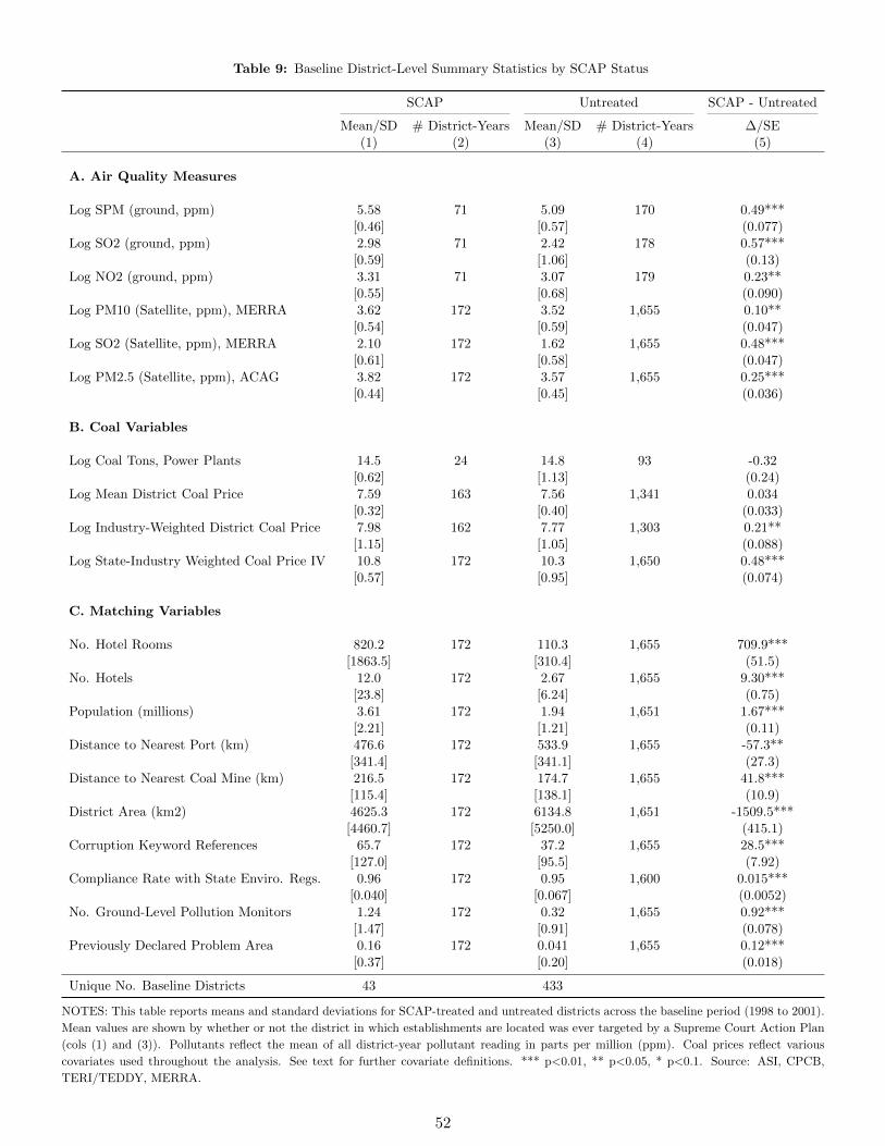
Table 9: Baseline District-Level Summary Statistics by SCAP Status

SCAP Untreated SCAP - Untreated

Mean/SD # District-Years Mean/SD # District-Years ∆/SE(1) (2) (3) (4) (5)

A. Air Quality Measures

Log SPM (ground, ppm) 5.58 71 5.09 170 0.49***[0.46] [0.57] (0.077)

Log SO2 (ground, ppm) 2.98 71 2.42 178 0.57***[0.59] [1.06] (0.13)

Log NO2 (ground, ppm) 3.31 71 3.07 179 0.23**[0.55] [0.68] (0.090)

Log PM10 (Satellite, ppm), MERRA 3.62 172 3.52 1,655 0.10**[0.54] [0.59] (0.047)

Log SO2 (Satellite, ppm), MERRA 2.10 172 1.62 1,655 0.48***[0.61] [0.58] (0.047)

Log PM2.5 (Satellite, ppm), ACAG 3.82 172 3.57 1,655 0.25***[0.44] [0.45] (0.036)

B. Coal Variables

Log Coal Tons, Power Plants 14.5 24 14.8 93 -0.32[0.62] [1.13] (0.24)

Log Mean District Coal Price 7.59 163 7.56 1,341 0.034[0.32] [0.40] (0.033)

Log Industry-Weighted District Coal Price 7.98 162 7.77 1,303 0.21**[1.15] [1.05] (0.088)

Log State-Industry Weighted Coal Price IV 10.8 172 10.3 1,650 0.48***[0.57] [0.95] (0.074)

C. Matching Variables

No. Hotel Rooms 820.2 172 110.3 1,655 709.9***[1863.5] [310.4] (51.5)

No. Hotels 12.0 172 2.67 1,655 9.30***[23.8] [6.24] (0.75)

Population (millions) 3.61 172 1.94 1,651 1.67***[2.21] [1.21] (0.11)

Distance to Nearest Port (km) 476.6 172 533.9 1,655 -57.3**[341.4] [341.1] (27.3)

Distance to Nearest Coal Mine (km) 216.5 172 174.7 1,655 41.8***[115.4] [138.1] (10.9)

District Area (km2) 4625.3 172 6134.8 1,651 -1509.5***[4460.7] [5250.0] (415.1)

Corruption Keyword References 65.7 172 37.2 1,655 28.5***[127.0] [95.5] (7.92)

Compliance Rate with State Enviro. Regs. 0.96 172 0.95 1,600 0.015***[0.040] [0.067] (0.0052)

No. Ground-Level Pollution Monitors 1.24 172 0.32 1,655 0.92***[1.47] [0.91] (0.078)

Previously Declared Problem Area 0.16 172 0.041 1,655 0.12***[0.37] [0.20] (0.018)

Unique No. Baseline Districts 43 433

NOTES: This table reports means and standard deviations for SCAP-treated and untreated districts across the baseline period (1998 to 2001).

Mean values are shown by whether or not the district in which establishments are located was ever targeted by a Supreme Court Action Plan

(cols (1) and (3)). Pollutants reflect the mean of all district-year pollutant reading in parts per million (ppm). Coal prices reflect various

covariates used throughout the analysis. See text for further covariate definitions. *** p<0.01, ** p<0.05, * p<0.1. Source: ASI, CPCB,

TERI/TEDDY, MERRA.

52

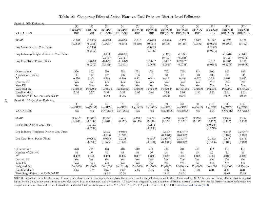
Table 10: Comparing Effect of Action Plans vs. Coal Prices on District-Level Pollutants

Panel A. DID Estimates(1) (2) (3) (4) (5) (6) (7) (8) (9) (10) (11) (12)

log(SPM) log(SPM) log(SPM) log(SPM) log(SO2) log(SO2) log(SO2) log(SO2) log(NO2) log(NO2) log(NO2) log(NO2)VARIABLES DID DID DID/2SLS DID/2SLS DID DID DID/2SLS DID/2SLS DID DID DID/2SLS DID/2SLS

SCAP -0.101 -0.0903 -0.0894 -0.0458 -0.116 -0.0889 -0.0895 -0.173 0.160* 0.166* 0.167* 0.101(0.0668) (0.0681) (0.0661) (0.101) (0.110) (0.111) (0.108) (0.116) (0.0882) (0.0920) (0.0866) (0.107)

Log Mean District Coal Price -0.0386 -0.0629 0.00599(0.0512) (0.0737) (0.0471)

Log Industry-Weighted District Coal Price 0.113 -0.0287 -0.120 -0.172* -0.0516 -0.160*(0.0857) (0.0847) (0.142) (0.0921) (0.102) (0.0935)

Log Coal Tons, Power Plants 0.00733 -0.0226 -0.00479 0.142** 0.183** 0.230*** 0.115 0.130* 0.105(0.0272) (0.0359) (0.0401) (0.0678) (0.0806) (0.0731) (0.0785) (0.0777) (0.0848)

Observations 836 800 796 794 794 768 762 760 843 809 805 803Number of District 111 110 107 106 105 104 98 97 110 109 105 104R2 0.390 0.391 0.380 0.366 0.231 0.248 0.248 0.249 0.037 0.044 0.049 0.022District FE Yes Yes Yes Yes Yes Yes Yes Yes Yes Yes Yes YesYear FE Yes Yes Yes Yes Yes Yes Yes Yes Yes Yes Yes YesWeighted By Pop2000 Pop2000 Pop2000 InitEstabs Pop2000 Pop2000 Pop2000 InitEstabs Pop2000 Pop2000 Pop2000 InitEstabs

Baseline Mean 5.55 5.57 5.57 5.57 2.95 2.96 2.96 2.96 3.30 3.31 3.31 3.31First Stage F-Stat. on Excluded IV 29.82 25.05 33.30 26.65 40.78 29.28

Panel B. NN-Matching Estimates(1) (2) (3) (4) (5) (6) (7) (8) (9) (10) (11) (12)

log(SPM) log(SPM) log(SPM) log(SPM) log(SO2) log(SO2) log(SO2) log(SO2) log(NO2) log(NO2) log(NO2) log(NO2)VARIABLES NN NN NN/2SLS NN/2SLS NN NN NN/2SLS NN/2SLS NN NN NN/2SLS NN/2SLS

SCAP -0.171** -0.170** -0.153* -0.210 -0.0817 -0.0741 -0.0979 -0.302** 0.0863 0.0890 0.0535 -0.117(0.0840) (0.0839) (0.0816) (0.152) (0.179) (0.176) (0.152) (0.123) (0.127) (0.132) (0.115) (0.126)

Log Mean District Coal Price -0.0123 -0.114 0.00233(0.0694) (0.0998) (0.0773)

Log Industry-Weighted District Coal Price 0.0892 -0.0308 -0.180* -0.204*** -0.255* -0.279***(0.115) (0.0991) (0.0981) (0.0660) (0.138) (0.101)

Log Coal Tons, Power Plants -0.00659 -0.0388 0.0108 0.158* 0.229*** 0.282*** 0.0422 0.137 0.176(0.0303) (0.0504) (0.0535) (0.0861) (0.0889) (0.0802) (0.0865) (0.103) (0.133)

Observations 420 413 413 413 412 406 404 404 419 412 411 411Number of District 46 46 46 46 46 46 44 44 45 45 44 44R2 0.432 0.429 0.439 0.395 0.337 0.360 0.333 0.280 0.028 0.030 -0.047 -0.030District FE Yes Yes Yes Yes Yes Yes Yes Yes Yes Yes Yes YesYear FE Yes Yes Yes Yes Yes Yes Yes Yes Yes Yes Yes YesWeighted By Pop2000 Pop2000 Pop2000 InitEstabs Pop2000 Pop2000 Pop2000 InitEstabs Pop2000 Pop2000 Pop2000 InitEstabs

Baseline Mean 5.55 5.57 5.57 5.57 2.95 2.96 2.96 2.96 3.30 3.31 3.31 3.31First Stage F-Stat. on Excluded IV 18.92 20.03 18.10 23.74 19.62 22.38

NOTES: Dependent variable reflects log of mean ground-level monitor readings within a given district and year for the pollutant shown in the column heading. SCAP is equal to 1 in any district that is targeted

for an Action Plan, in any year during or after the Action Plan is announced, and 0 otherwise. All regressions weighted by initial number of firms in district in 1998. See text for further covariate definitions and

sample restrictions. Standard errors clustered at the district level, shown in parentheses. *** p<0.01, ** p<0.05, * p<0.1. Source: ASI, CPCB, Greenstone and Hanna (2014).

53

References

Abadie, A., D. Drukker, J. L. Herr, and G. W. Imbens (2004): “Implementing Matching Estima-tors for Average Treatment Effects in Stata,” The Stata Journal, 4, 290–311.

Abadie, A. and G. W. Imbens (2002): “Simple and Bias-Corrected Matching Estimators for AverageTreatment Effects,” NBER Technical Working Paper, 283.

Ackerberg, D. A., K. Caves, and G. Frazer (2006): “Structural Identification of ProductionFunctions,” Mimeo.

Angrist, J. D., G. W. Imbens, and A. B. Krueger (1999): “Jackknife Instrumental VariablesEstimation,” Journal of Applied Econometrics, 14, 57–67.

Angrist, J. D., G. W. Imbens, and D. B. Rubin (1996): “Identification of causal effects usinginstrumental variables,” Journal of the American statistical Association, 91, 444–455.

Angrist, J. D. and J.-S. Pischke (2008): Mostly harmless econometrics: An empiricist’s companion,Princeton university press.

Becker, R. and V. Henderson (2000): “Effects of Air Quality Regulations on Polluting Industries,”Journal of Political Economy, 108, 379–421.

Bertrand, M., S. Djankov, R. Hanna, and S. Mullainathan (2007): “Obtaining a Driver’s Licensein India: an Experimental Approach to Studying Corruption,” The Quarterly Journal of Economics,122, 1639–1676.

Blackman, A. and W. Harrington (2000): “The Use of Economic Incentives in Developing Countries:Lessons from International Experience with Industrial Air Pollution,” The Journal of Environment &Development, 9, 5–44.

Chetty, R., A. Looney, and K. Kroft (2009): “Salience and Taxation: Theory and Evidence,”American Economic Review, 99, 1145–1177.

Chikkatur, A. P. (2008): “A resource and technology assessment of coal utilization in India,” Tech.rep., Pew Center on Global Climate Change, Arlington, VA (United States).

Chodorow-Reich, G., L. Feiveson, Z. Liscow, and W. G. Woolston (2013): “Does State FiscalRelief during Recessions Increase Employment? Evidence from the American Recovery and Reinvest-ment Act,” American Economic Journal: Economic Policy, 4, 118–145.

CPCB (2009): “Comprehensive Environmental Assessment of Industrial Clusters,” Ecological ImpactAssessment Series EIAS/5/2009–2010, Ministry of Environment and Forests.

Duflo, E., M. Greenstone, R. Pande, and N. Ryan (2013): “Truth-Telling by Third-Party Auditorsand the Response of Polluting Firms: Experimental Evidence from India,” The Quarterly Journal ofEconomics, 128, 1499–1545.

——— (2014): “The Value of Regulatory Discretion: Estimates from Environmental Inspections in India,”NBER Working Paper, 20590.

EIA, U. (2012): “Fuel competition in power generation and elasticities of substitution,” USEnergy Information Administration. https://www. eia. gov/analysis/studies/fuelelasticities/pdf/eia-fuelelasticities.pdf.

Estache, A. and L. Wren-Lewis (2009): “Toward a Theory of Regulation for Developing Countries:Following Jean-Jacques Laffont’s Lead,” Journal of Economic Literature, 47, 729–770.

54

Greenstone, M. and R. Hanna (2014): “Environmental Regulations, Air and Water Pollution, andInfant Mortality in India,” American Economic Review, 104, 3038–3072.

Greenstone, M., J. A. List, and C. Syverson (2012): “The Effects of Environmental Regulationon the Competitiveness of U.S. Manufacturing,” NBER Working Paper, 18392.

Hausman, J. A. (1996): “Valuation of New Goods Under Perfect and Imperfect Competition,” in TheEconomics of New Goods, ed. by T. F. Bresnahan and R. J. Gordon, Chicago, IL: NBER University ofChicago Press, 207–248.

Heckman, J. J., H. Ichimura, and P. E. Todd (1997): “Matching as an Econometric EvaluationEstimator: Evidence from Evaluating a Job Training Programme,” The Review of Economic Studies,64, 605–654.

Henderson, J. V. (1996): “Effects of air quality regulation,” The American Economic Review, 86, 789.

Hyman, B. G. (2018): “Can Displaced Labor Be Retrained? Evidence from Quasi-Random Assignmentto Trade Adjustment Assistance,” .

IISD (2017): “India’s Energy Transition - Mapping Subsidies to Fossil Fuels and Clean Energy in India,”.

Imbens, G. W. (2004): “Nonparametric Estimation of Average Treatment Effects under Exogeneity: AReview,” Review of Economics and Statistics, 86, 4–29.

International Energy Agency (2018): World Energy Outlook 2018, Paris: OECD/IEA.

Jaffe, A. B. and K. Palmer (1997): “Environmental Regulation and Innovation: A Panel DataStudy,” Review of Economics and Statistics, 79, 610–619.

King, G. and R. Nielsen (2016): “Why Propensity Scores Should Not be Used for Matching,” PoliticalAnalysis, 1–20.

Laffont, J.-J. (2005): Regulation and Development, Cambridge University Press.

Lanjouw, J. and A. Mody (1996): “Innovation and the international diffusion of environmentallyresponsive technology,” Research Policy, 25, 549–571.

Levinsohn, J. and A. Petrin (2003): “Estimating Production Functions using Inputs to Control forUnobservables,” The Review of Economic Studies, 70, 317–341.

Levinson, A. (1996): “Environmental regulations and manufacturers’ location choices: Evidence fromthe Census of Manufactures,” Journal of public Economics, 62, 5–29.

Linn, J. (2008): “Energy Prices and the Adoption of Energy-Saving Technology,” The Economic Journal,118, 1986–2012.

List, J. A., D. L. Millimet, P. G. Fredriksson, and W. W. McHone (2003): “Effects of Envi-ronmental Regulations on Manufacturing Plant Births: Evidence from a Propensity Score MatchingEstimator,” Review of Economics and Statistics, 85, 944–952.

Liu, M. and L. Martin (2014): “When Giants Take Steps: The Impact of Conservation Targets onChina’s Largest Energy-Consuming Firms,” University of Melbourne Working Paper.

Martin, L. A., S. Nataraj, and A. Harrison (2014): “In With the Big, Out With the Small:Removing Small-Scale Reservations in India,” NBER Working Paper, 19942.

Millimet, D. L. and J. Roy (2016): “Empirical tests of the pollution haven hypothesis when environ-mental regulation is endogenous,” Journal of Applied Econometrics, 31, 652–677.

55

Newell, R. G., A. B. Jaffe, and R. N. Stavins (1999): “The Induced Innovation Hypothesis andEnergy-Saving Technological Change,” Quarterly Journal of Economics, 114, 941–975.

Olley, G. S. and A. Pakes (1996): “The Dynamics of Productivity in the Telecommunications Equip-ment Industry,” Econometrica, 64, 1263–1297.

Popp, D. (2002): “Induced Innovation and Energy Prices,” American Economic Review, 92, 160–180.

Serletis, A., G. R. Timilsina, and O. Vasetsky (2010): “Interfuel substitution in the United States,”Energy Economics, 32, 737–745.

Tanaka, S., W. Yin, and G. H. Jefferson (2014): “Environmental Regulation and Industrial Per-formance: Evidence from China,” Mimeo.

Tongia, R. and S. Gross (2019): “Coal in India: Adjusting to transition,” .

Van Donkelaar, A., R. V. Martin, M. Brauer, N. C. Hsu, R. A. Kahn, R. C. Levy, A. Lya-pustin, A. M. Sayer, and D. M. Winker (2016): “Global estimates of fine particulate matter usinga combined geophysical-statistical method with information from satellites, models, and monitors,” En-vironmental science & technology, 50, 3762–3772.

Walker, W. R. (2013): “The Transitional Costs of Sectoral Reallocation: Evidence from the Clean AirAct and the Workforce,” Quarterly Journal of Economics, 128, 1787–1835.

56

Appendices

Appendix A. Detailed Policy Variation

A.1 Supreme Court Action Plan, Selected Policy Detail

This appendix provides selected details on each city action plan according to the primary source “Air QualityTrends and Action Plan for Control of Air Pollution from Seventeen Cities” (CPCB & MoEF, September 2006)

Delhi (1997-1998):

• Relocation of 46 Hot Mix Plants and relocation of 243 Brick Kilns• Establishment of 15 Common Effluent Treatment Plants (CETPs) in industrial areas• 3 coal-based power plants to switch to beneficiated coal

Agra (2002):

• Five zone implementation plan of Compressed Natural Gas (CNG) devised, including CNG/LPG (liquefiedPetroleum Gas) stations and natural gas pipelines via GAIL network• Restrictions on the supply and usage of coal, coke, wood, rice husk, bagasse to all industries• Diesel generator sets in no-gas zones to be fitted with wet scrubbers or replaced by gas generators• Enforced Supreme Court directorate of 292 industries (plants) 46 not to use coal or coke• Supreme court directed closure of Brick Kilns in Trapezium Zone• Conversion of all 3 wheelers, temp, rickshaws, taxis, buses to CNG/LPG in phases in accordance with

Supreme Court directive. In the interim, fit these vehicles with wet scrubbers / filters

Ahmedabad (2002):

• 1595 industrial units are now monitored per the Air Act, including 150 wet scrubbers and 2 ESP (elec-trostatic precipitators). Resulted in 27 closures and 501 warnings• Plan devised for Highly Polluting Industries (HPIs) to switch over to natural gas, affecting 146 industries

with major boilers, and 500 foundries. 190 units signed up• No new four wheelers registered without being compliant with Bharat Stage II norms• Formalization of all rickshaws, and addition of fueling stations planned. All diesel-run rickshaws within

city limits are banned

Calcutta (2002):

• Stricter location policy for new industrial units in red category• Restrictions on coal supply to certain industries and mandatory use of clean fuels• Financial assistance for pollution control devices for SSIs• ESPs in all 6 boilers in new Cossipore Generation Station• Stricter inspection schedule and standards, by West Bengal Pollution Control Board.• Stricter standards for coal fired boilers, ceramic kilns, hot rolling mills, and small cast iron foundries

Dhanbad (Jharia) (2002):

• Compliance with diesel generator set standards• All petrol and diesel to conform to Bharat Stage III norms• Construction of flyovers (pedestrian overpasses) and Bus Rapid Transit Systems (BRTSs)

46Indian convention uses the word “industries” to refer to plants or establishments

57

Faridabad (2002):

• Closure of clandestine units and promotion of natural gas inputs (i.e. CNG, Light Diesel Oil, and HighSpeed Diesel)• Ultra low sulfur diesel to be used in generating sets• Thermal Power Plants should keep ESPs

Jodhpur (2002):

• Master plan to shift various commercial activities in dense areas outside of the city• Development of a Green Belt around the city• Reduction in sulfur diesel content

Kanpur (2002):

• Shifting of polluting industries and installation of pollution control devices• GAIL (largest preferentially-contracted natural gas company in India) to supply .3837 MMSCMD of

natural gas by 2006, and continues to expand pipeline into Kanpur• Development of Green Belt around the city• No new industries allowed to locate in residential centers• Only allow three-wheelers with catalytic converters to operate within municipal limits• Phase out of old vehicles, and import of 250 CNG buses to take their place is planned

Lucknow (2002):

• ESPs (electrostatic precipitators) to be installed in all boilers in power generation stations• Stricter regulation of medium/large industries in technical hearings and stricter emissions standards for

SSIs operating coal fired boilers, ceramic kilns, hot rolling mills, and small cast iron foundries• New emissions norms for diesel engines phased in Jan-July 2004

Patna (2002):

• Intensification of Air Act norms including through surprise inspections and new punitive action• Establishment of a green belt around all industrial units in the city• Elimination of Kerosene in vehicles (including 3-wheelers and commercial vehicles) by March 2004• Mandated compliance with Bharat Stage II norms

Pune (2002):

• Closure of clandestine industrial operations or shifting• Compliance to standards in diesel generator sets• Implementation of industrial location policy for shifting of industries from non-conforming zones• The Ministry of Petroleum and Natural Gas (MoPNG) allocated 0.4 MMSCMD of Administered Price

Mechanism (APM) gas which would be cheaper than the gas bought from the private players• GAIL’s proposed Dahej-Uran Pipeline (DUPL) will be extended up to Pune

Varanasi (2002):

• Monitoring and closure of clandestine operations• Retrofitting of catalytic converters• Mandate of new emissions norms for low Benzene and low sulfur diesel

58

Bangalore (2003):

• Established Karnataka State Pollution Control Board online ambient air quality monitoring station• 108 roads converted to one-way, 5 flyovers, 3 railway passes

Chennai (2003):

• All smoke stacks require an online monitor and are subject to increased inspection• Common facilities set up outside of the city for incineration of bio-medical waste• Coal handling shifted entirely from Chennai port to Ennore Port by December 2004• Provided scrubbers to reduce emissions to power plants• 117 buses to be replaced with Bharat Stage II adherence

Hyderabad (2003):

• Closure of clandestine units and stricter regulation and inspection• Promotion of alternative fuels, including only use of ultra-low sulfur in generating sets• Thermal power plants to keep using ESPs• Increasing bus fleet with grant to allocate 2,476 new bus permits

Mumbai (2003):

• All DG sets must have a phase-in plan to meet emission norms by July 2004.• Supreme Court mandated stone crushing and hot mix plants to move out of Kandivili in 2003• Corporate Responsibility for Environmental Protection (PCREP) for highly polluting industries will be

required and monitored in a time bound manner• Increase CNG dispensing stations from 67 to 80 by March, 2004

Solapur (2003):

• No stone crushes within 500 meters of highways or rivers or residential habitations.• Compliance with diesel generator set standards.• Corporate Responsibility for Environmental Protection (CREP) for highly polluting industries adopted

and monitored.• 6-seater rickshaws banned. No new rickshaws can have diesel.• Ban on 2-T oil, and vehicles checked regularly for PUC certificate.

59

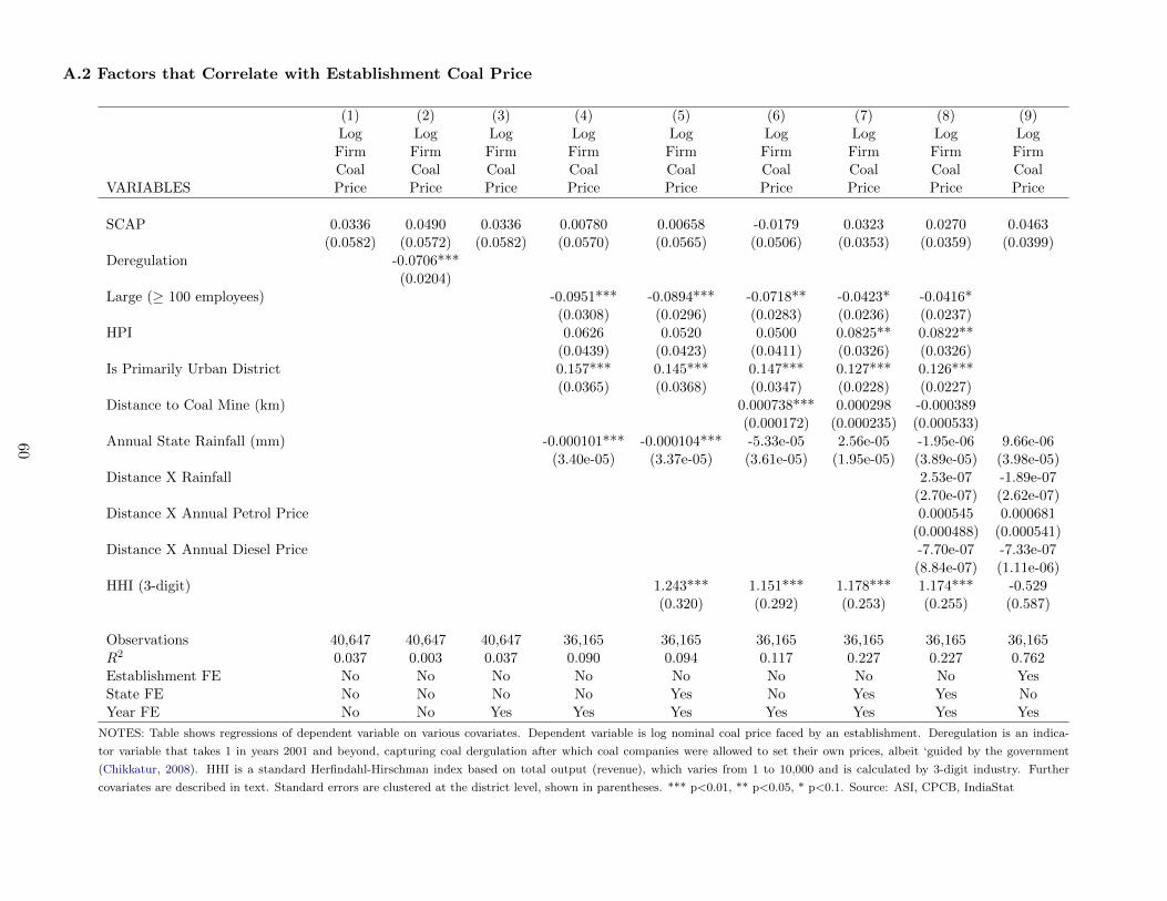
A.2 Factors that Correlate with Establishment Coal Price

(1) (2) (3) (4) (5) (6) (7) (8) (9)Log Log Log Log Log Log Log Log LogFirm Firm Firm Firm Firm Firm Firm Firm FirmCoal Coal Coal Coal Coal Coal Coal Coal Coal

VARIABLES Price Price Price Price Price Price Price Price Price

SCAP 0.0336 0.0490 0.0336 0.00780 0.00658 -0.0179 0.0323 0.0270 0.0463(0.0582) (0.0572) (0.0582) (0.0570) (0.0565) (0.0506) (0.0353) (0.0359) (0.0399)

Deregulation -0.0706***(0.0204)

Large (≥ 100 employees) -0.0951*** -0.0894*** -0.0718** -0.0423* -0.0416*(0.0308) (0.0296) (0.0283) (0.0236) (0.0237)

HPI 0.0626 0.0520 0.0500 0.0825** 0.0822**(0.0439) (0.0423) (0.0411) (0.0326) (0.0326)

Is Primarily Urban District 0.157*** 0.145*** 0.147*** 0.127*** 0.126***(0.0365) (0.0368) (0.0347) (0.0228) (0.0227)

Distance to Coal Mine (km) 0.000738*** 0.000298 -0.000389(0.000172) (0.000235) (0.000533)

Annual State Rainfall (mm) -0.000101*** -0.000104*** -5.33e-05 2.56e-05 -1.95e-06 9.66e-06(3.40e-05) (3.37e-05) (3.61e-05) (1.95e-05) (3.89e-05) (3.98e-05)

Distance X Rainfall 2.53e-07 -1.89e-07(2.70e-07) (2.62e-07)

Distance X Annual Petrol Price 0.000545 0.000681(0.000488) (0.000541)

Distance X Annual Diesel Price -7.70e-07 -7.33e-07(8.84e-07) (1.11e-06)

HHI (3-digit) 1.243*** 1.151*** 1.178*** 1.174*** -0.529(0.320) (0.292) (0.253) (0.255) (0.587)

Observations 40,647 40,647 40,647 36,165 36,165 36,165 36,165 36,165 36,165R2 0.037 0.003 0.037 0.090 0.094 0.117 0.227 0.227 0.762Establishment FE No No No No No No No No YesState FE No No No No Yes No Yes Yes NoYear FE No No Yes Yes Yes Yes Yes Yes Yes

NOTES: Table shows regressions of dependent variable on various covariates. Dependent variable is log nominal coal price faced by an establishment. Deregulation is an indica-

tor variable that takes 1 in years 2001 and beyond, capturing coal dergulation after which coal companies were allowed to set their own prices, albeit ‘guided by the government

(Chikkatur, 2008). HHI is a standard Herfindahl-Hirschman index based on total output (revenue), which varies from 1 to 10,000 and is calculated by 3-digit industry. Further

covariates are described in text. Standard errors are clustered at the district level, shown in parentheses. *** p<0.01, ** p<0.05, * p<0.1. Source: ASI, CPCB, IndiaStat

60

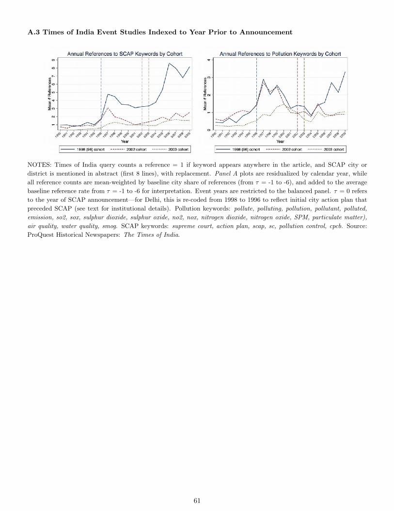
A.3 Times of India Event Studies Indexed to Year Prior to Announcement

NOTES: Times of India query counts a reference = 1 if keyword appears anywhere in the article, and SCAP city or

district is mentioned in abstract (first 8 lines), with replacement. Panel A plots are residualized by calendar year, while

all reference counts are mean-weighted by baseline city share of references (from τ = -1 to -6), and added to the average

baseline reference rate from τ = -1 to -6 for interpretation. Event years are restricted to the balanced panel. τ = 0 refers

to the year of SCAP announcement—for Delhi, this is re-coded from 1998 to 1996 to reflect initial city action plan that

preceded SCAP (see text for institutional details). Pollution keywords: pollute, polluting, pollution, pollutant, polluted,

emission, so2, sox, sulphur dioxide, sulphur oxide, no2, nox, nitrogen dioxide, nitrogen oxide, SPM, particulate matter),

air quality, water quality, smog. SCAP keywords: supreme court, action plan, scap, sc, pollution control, cpcb. Source:

ProQuest Historical Newspapers: The Times of India.

61

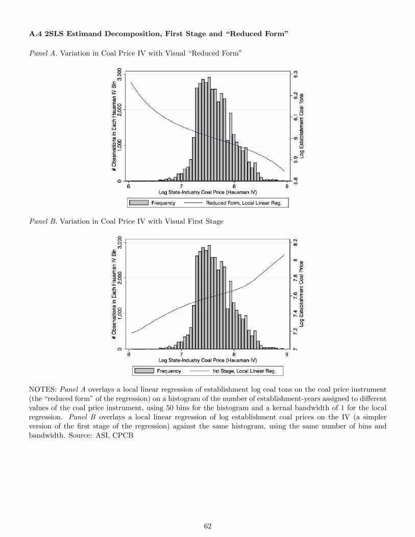
A.4 2SLS Estimand Decomposition, First Stage and “Reduced Form”

Panel A. Variation in Coal Price IV with Visual “Reduced Form”

Panel B. Variation in Coal Price IV with Visual First Stage

NOTES: Panel A overlays a local linear regression of establishment log coal tons on the coal price instrument(the “reduced form” of the regression) on a histogram of the number of establishment-years assigned to differentvalues of the coal price instrument, using 50 bins for the histogram and a kernal bandwidth of 1 for the localregression. Panel B overlays a local linear regression of log establishment coal prices on the IV (a simplerversion of the first stage of the regression) against the same histogram, using the same number of bins andbandwidth. Source: ASI, CPCB

62

Appendix B. Nearest Neighbor Matching Appendices

B.1 Nearest Neighbor Matching Estimation Procedure

While the main difference-in-differences (DID) strategy discussed above provides suggestive evidence that theDID common trends absent treatment assumption is valid, flat pre-trends are but a necessary and not sufficientcondition for identification. Though Times of India references indicated the timing of Supreme Court ActionPlan (SCAP) announcements was unanticipated, one remaining concern is that regulators may target the citiesthemselves based on cross-sectional factors unobserved to the econometrician. Noisy covariates and unobservedheterogeneity may generate seemingly-flat pre-trends in the dependent variable, but confound estimates in thepost-treatment period when not accounted for properly. Imbens (2004) refers to these problems as covariateoverlap and unconfoundedness respectively.

To gauge the robustness of our results to this limitation, we present an alternative matched-sample strategythroughout the draft in which we use a nearest-neighbor (NN) matching procedure to pair each SCAP-treatedunit in our sample with an untreated unit, and run our standard difference-in-differences estimator usingthis newly matched control group in place of the default control group (untreated establishments at timeof treatment)47. Intuitively, in establishment-level analyses, our matching estimator finds establishments inuntreated districts with similar district characteristics to SCAP districts, however imposes that establishmentsbe matched exactly within each of the four HPI x Size subgroups (which vary by establishment). In district-levelanalysis, we match only on district-level variables (the full set of matching covariates for both strategies is listedbelow).

We use the semiparametic estimator described in Abadie and Imbens (2002). Starting with establishment-level results, we desire an establishment-level treatment effect for each treated observation i, θi = Yi(1)Yi(0),but only one potential outcome is observable for each unit. We consider a distance metric ||XiXj || that createsa score between a treated units covariates Xi and all potential j control candidates with covariate vectors Xj inthe years prior to SCAP announcement (1998 to 2001), and keep the closest Mi matches for each treated uniti48. To equalize scales among the different components of each vector in their contribution to the distance score,we use a Mahalanobis distance statistic—weighting vector distances by the inverse of the variance-covariancematrix (Σ) for covariates:

||XiXj ||Mahalanobis =

√(XiXj)(Σ

−1x )(XiXj) (5)

We use the algorithm discussed in Abadie et al. (2004) to implement this procedure for both establishment-and district-level regressions. This procedure has the useful property that violators of the covariate overlapassumption are dropped, resulting in treated units only being used if the covariates share a sufficiently commoncovariate support. While our algorithm results in no such dropped units, we also show in Appendix B.2,predicted SCAP status balance in each of the four subgroups, suggesting that indeed there is ample mass acrossthe support for treated units to find close nearest neighbors, circumventing problems arising from high-distancenearest neighbors in which covariates are not evenly distributed (a critique recently popularized by King andNielsen (2016), which partly guided our decision to use a nearest-neighbor matching algorithm which does notcollapse information into a single coarse metric, such as a propensity score).49 Finally, in Appendix B.3 below,the NN necessary condition of flat pretends appears to be met visually.

47In regression tables, we use the header NN to distinguish this strategy from DID, though a more apt name is matched difference-in-difference estimator” (Heckman et al., 1997).

48In practice, we choose to use only one nearest neighbor, making the potential outcome problem symmetric. We allow treatedunits to match to different control units in each of the baseline years (1998 to 2001), and probability weight all regressions by thenumber of times a control unit is matched. To ensure that there are no ties in a given year, we include Log(Output) as a matchingvariable. Results are nearly equivalent when omitting Log(Output) as a matching variableits function is mainly as a high-variation,highly-populated variable by establishment and year.

49In these overlap pictures, the main interest is to ensure that there are no notable gaps in any point in the distribution.

63

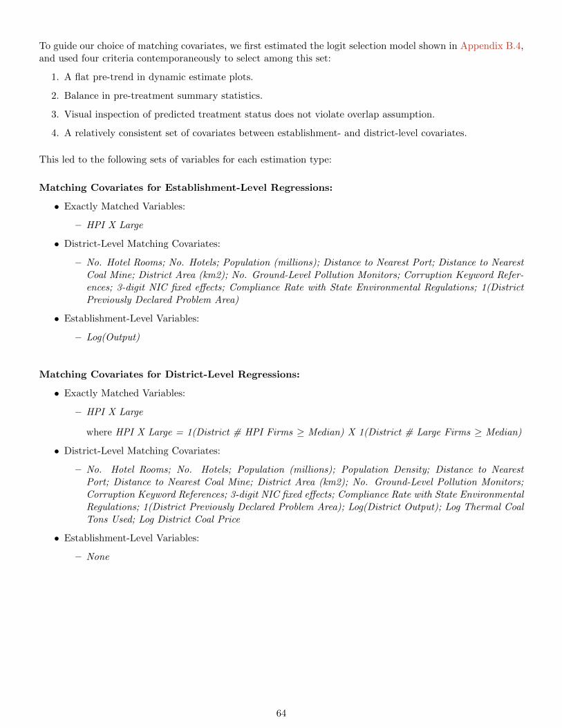
To guide our choice of matching covariates, we first estimated the logit selection model shown in Appendix B.4,and used four criteria contemporaneously to select among this set:

1. A flat pre-trend in dynamic estimate plots.

2. Balance in pre-treatment summary statistics.

3. Visual inspection of predicted treatment status does not violate overlap assumption.

4. A relatively consistent set of covariates between establishment- and district-level covariates.

This led to the following sets of variables for each estimation type:

Matching Covariates for Establishment-Level Regressions:

• Exactly Matched Variables:

– HPI X Large

• District-Level Matching Covariates:

– No. Hotel Rooms; No. Hotels; Population (millions); Distance to Nearest Port; Distance to NearestCoal Mine; District Area (km2); No. Ground-Level Pollution Monitors; Corruption Keyword Refer-ences; 3-digit NIC fixed effects; Compliance Rate with State Environmental Regulations; 1(DistrictPreviously Declared Problem Area)

• Establishment-Level Variables:

– Log(Output)

Matching Covariates for District-Level Regressions:

• Exactly Matched Variables:

– HPI X Large

where HPI X Large = 1(District # HPI Firms ≥ Median) X 1(District # Large Firms ≥ Median)

• District-Level Matching Covariates:

– No. Hotel Rooms; No. Hotels; Population (millions); Population Density; Distance to NearestPort; Distance to Nearest Coal Mine; District Area (km2); No. Ground-Level Pollution Monitors;Corruption Keyword References; 3-digit NIC fixed effects; Compliance Rate with State EnvironmentalRegulations; 1(District Previously Declared Problem Area); Log(District Output); Log Thermal CoalTons Used; Log District Coal Price

• Establishment-Level Variables:

– None

64

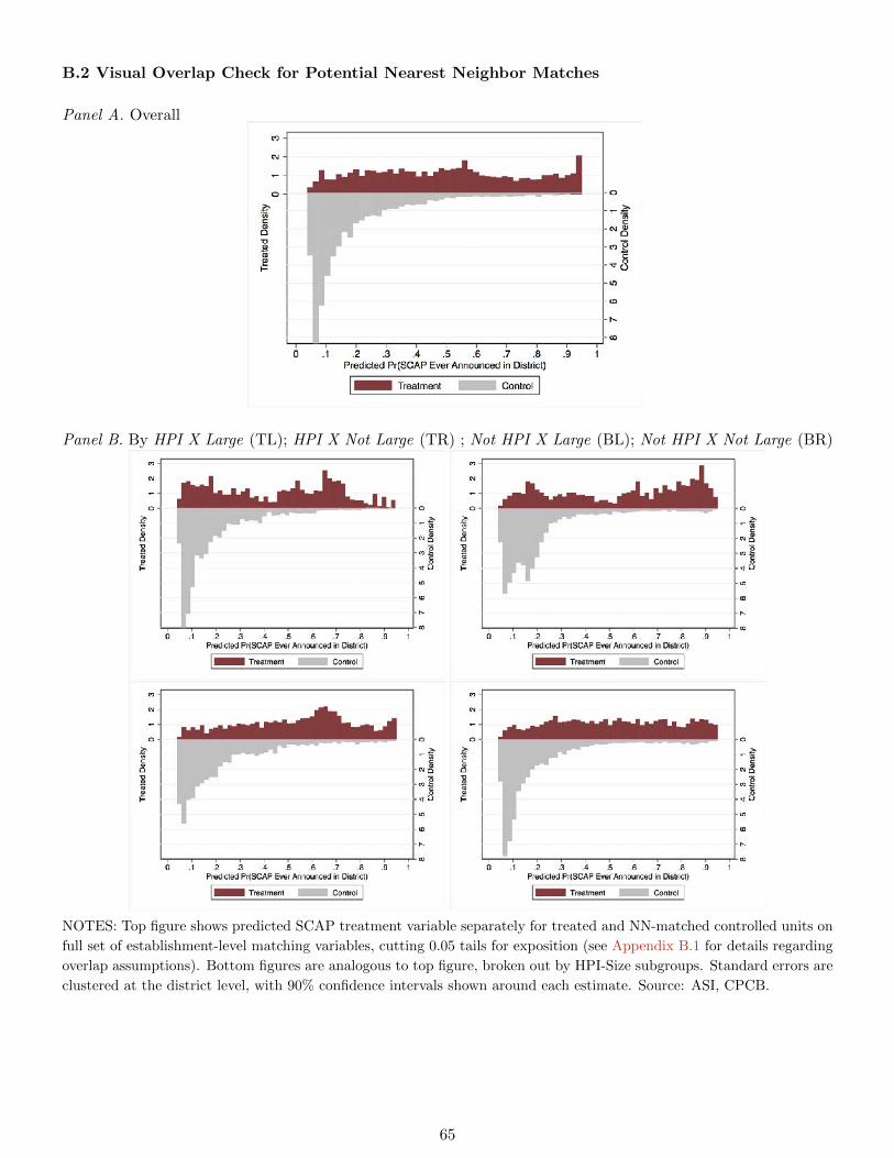
B.2 Visual Overlap Check for Potential Nearest Neighbor Matches

Panel A. Overall

Panel B. By HPI X Large (TL); HPI X Not Large (TR) ; Not HPI X Large (BL); Not HPI X Not Large (BR)

NOTES: Top figure shows predicted SCAP treatment variable separately for treated and NN-matched controlled units on

full set of establishment-level matching variables, cutting 0.05 tails for exposition (see Appendix B.1 for details regarding

overlap assumptions). Bottom figures are analogous to top figure, broken out by HPI-Size subgroups. Standard errors are

clustered at the district level, with 90% confidence intervals shown around each estimate. Source: ASI, CPCB.

65

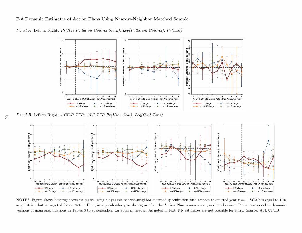
B.3 Dynamic Estimates of Action Plans Using Nearest-Neighbor Matched Sample

Panel A. Left to Right: Pr(Has Pollution Control Stock); Log(Pollution Control); Pr(Exit)

Panel B. Left to Right: ACF-P TFP; OLS TFP Pr(Uses Coal); Log(Coal Tons)

NOTES: Figure shows heterogeneous estimates using a dynamic nearest-neighbor matched specification with respect to omitted year τ =-1. SCAP is equal to 1 in

any district that is targeted for an Action Plan, in any calendar year during or after the Action Plan is announced, and 0 otherwise. Plots correspond to dynamic

versions of main specifications in Tables 3 to 9, dependent variables in header. As noted in text, NN estimates are not possible for entry. Source: ASI, CPCB

66

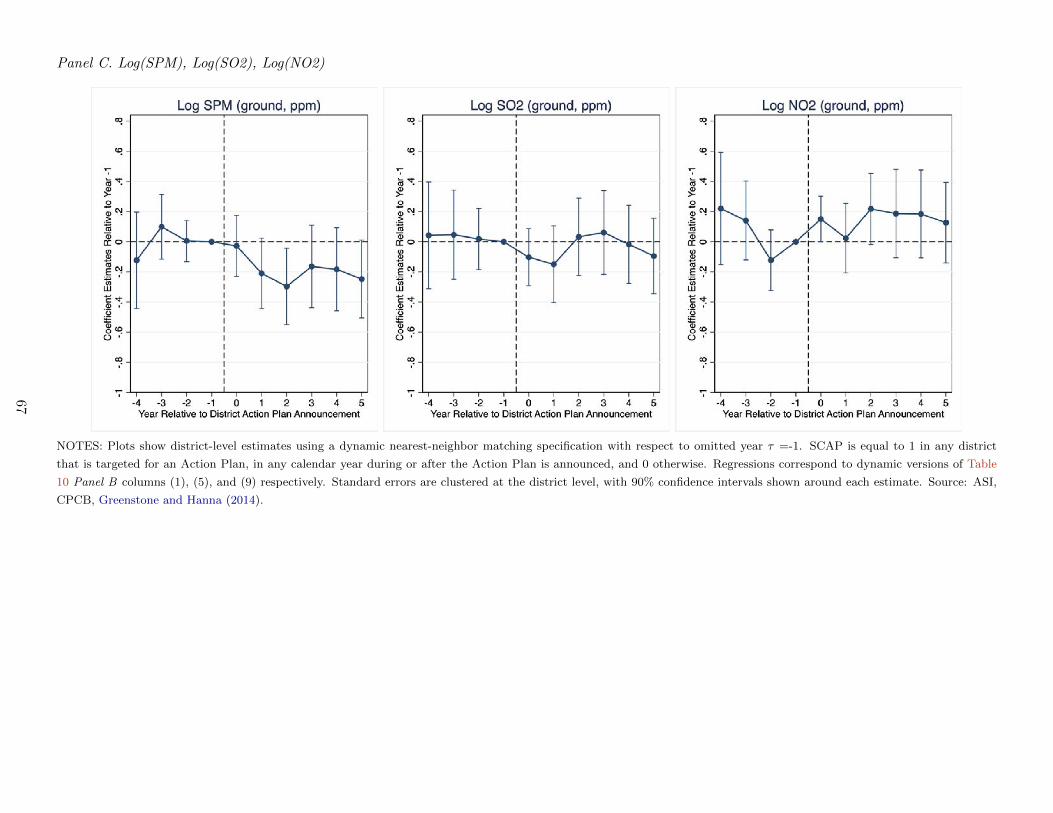
Panel C. Log(SPM), Log(SO2), Log(NO2)

NOTES: Plots show district-level estimates using a dynamic nearest-neighbor matching specification with respect to omitted year τ =-1. SCAP is equal to 1 in any district

that is targeted for an Action Plan, in any calendar year during or after the Action Plan is announced, and 0 otherwise. Regressions correspond to dynamic versions of Table

10 Panel B columns (1), (5), and (9) respectively. Standard errors are clustered at the district level, with 90% confidence intervals shown around each estimate. Source: ASI,

CPCB, Greenstone and Hanna (2014).

67

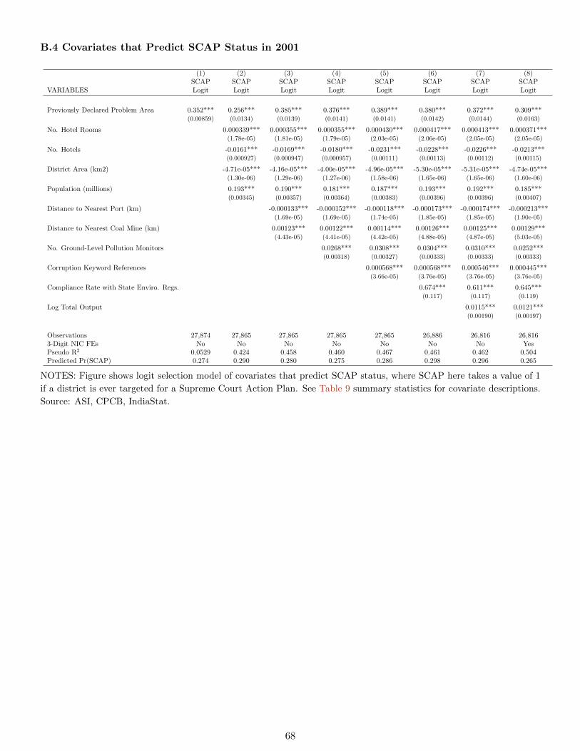
B.4 Covariates that Predict SCAP Status in 2001

(1) (2) (3) (4) (5) (6) (7) (8)SCAP SCAP SCAP SCAP SCAP SCAP SCAP SCAP

VARIABLES Logit Logit Logit Logit Logit Logit Logit Logit

Previously Declared Problem Area 0.352*** 0.256*** 0.385*** 0.376*** 0.389*** 0.380*** 0.372*** 0.309***(0.00859) (0.0134) (0.0139) (0.0141) (0.0141) (0.0142) (0.0144) (0.0163)

No. Hotel Rooms 0.000339*** 0.000355*** 0.000355*** 0.000430*** 0.000417*** 0.000413*** 0.000371***(1.78e-05) (1.81e-05) (1.79e-05) (2.03e-05) (2.06e-05) (2.05e-05) (2.05e-05)

No. Hotels -0.0161*** -0.0169*** -0.0180*** -0.0231*** -0.0228*** -0.0226*** -0.0213***(0.000927) (0.000947) (0.000957) (0.00111) (0.00113) (0.00112) (0.00115)

District Area (km2) -4.71e-05*** -4.16e-05*** -4.00e-05*** -4.96e-05*** -5.30e-05*** -5.31e-05*** -4.74e-05***(1.30e-06) (1.29e-06) (1.27e-06) (1.58e-06) (1.65e-06) (1.65e-06) (1.60e-06)

Population (millions) 0.193*** 0.190*** 0.181*** 0.187*** 0.193*** 0.192*** 0.185***(0.00345) (0.00357) (0.00364) (0.00383) (0.00396) (0.00396) (0.00407)

Distance to Nearest Port (km) -0.000133*** -0.000152*** -0.000118*** -0.000173*** -0.000174*** -0.000213***(1.69e-05) (1.69e-05) (1.74e-05) (1.85e-05) (1.85e-05) (1.90e-05)

Distance to Nearest Coal Mine (km) 0.00123*** 0.00122*** 0.00114*** 0.00126*** 0.00125*** 0.00129***(4.43e-05) (4.41e-05) (4.42e-05) (4.88e-05) (4.87e-05) (5.03e-05)

No. Ground-Level Pollution Monitors 0.0268*** 0.0308*** 0.0304*** 0.0310*** 0.0252***(0.00318) (0.00327) (0.00333) (0.00333) (0.00333)

Corruption Keyword References 0.000568*** 0.000568*** 0.000546*** 0.000445***(3.66e-05) (3.76e-05) (3.76e-05) (3.76e-05)

Compliance Rate with State Enviro. Regs. 0.674*** 0.611*** 0.645***(0.117) (0.117) (0.119)

Log Total Output 0.0115*** 0.0121***(0.00190) (0.00197)

Observations 27,874 27,865 27,865 27,865 27,865 26,886 26,816 26,8163-Digit NIC FEs No No No No No No No YesPseudo R2 0.0529 0.424 0.458 0.460 0.467 0.461 0.462 0.504Predicted Pr(SCAP) 0.274 0.290 0.280 0.275 0.286 0.298 0.296 0.265

NOTES: Figure shows logit selection model of covariates that predict SCAP status, where SCAP here takes a value of 1

if a district is ever targeted for a Supreme Court Action Plan. See Table 9 summary statistics for covariate descriptions.

Source: ASI, CPCB, IndiaStat.

68

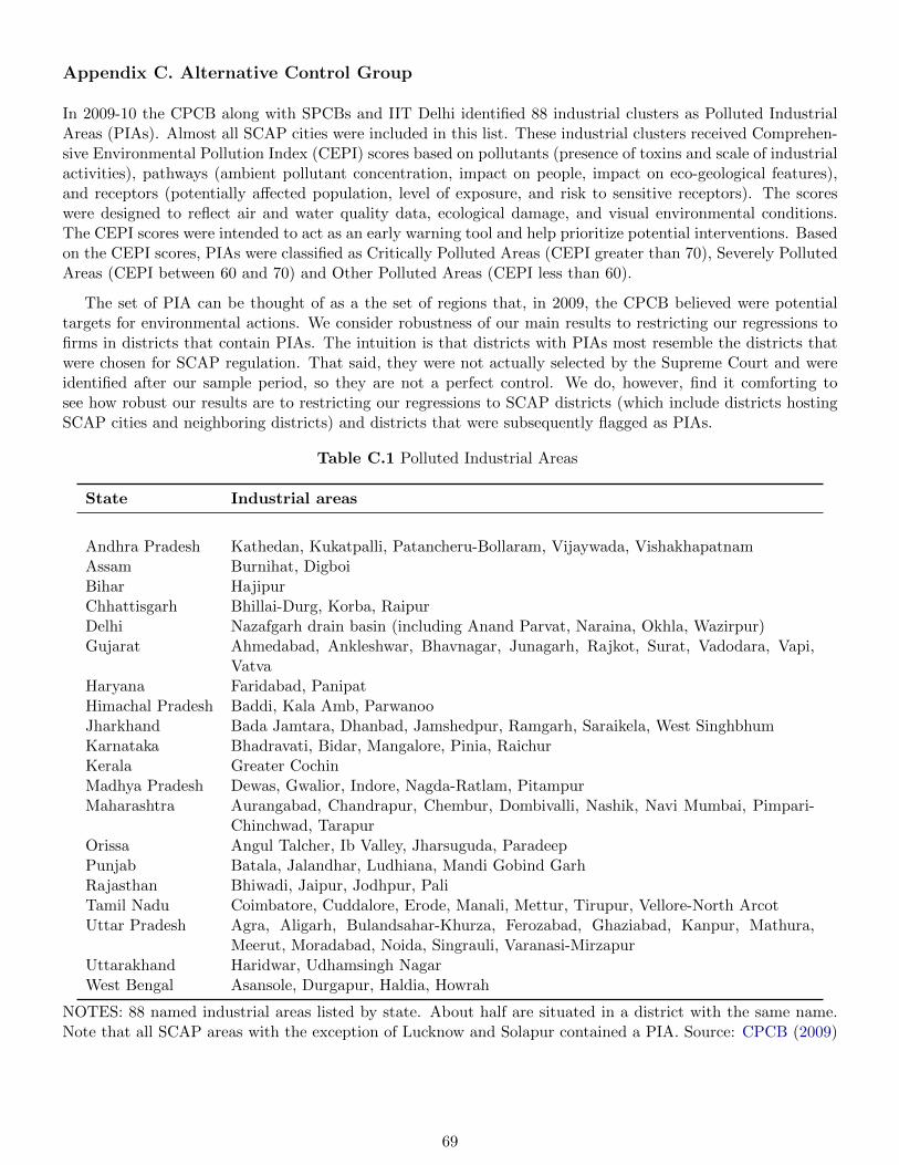
Appendix C. Alternative Control Group

In 2009-10 the CPCB along with SPCBs and IIT Delhi identified 88 industrial clusters as Polluted IndustrialAreas (PIAs). Almost all SCAP cities were included in this list. These industrial clusters received Comprehen-sive Environmental Pollution Index (CEPI) scores based on pollutants (presence of toxins and scale of industrialactivities), pathways (ambient pollutant concentration, impact on people, impact on eco-geological features),and receptors (potentially affected population, level of exposure, and risk to sensitive receptors). The scoreswere designed to reflect air and water quality data, ecological damage, and visual environmental conditions.The CEPI scores were intended to act as an early warning tool and help prioritize potential interventions. Basedon the CEPI scores, PIAs were classified as Critically Polluted Areas (CEPI greater than 70), Severely PollutedAreas (CEPI between 60 and 70) and Other Polluted Areas (CEPI less than 60).

The set of PIA can be thought of as a the set of regions that, in 2009, the CPCB believed were potentialtargets for environmental actions. We consider robustness of our main results to restricting our regressions tofirms in districts that contain PIAs. The intuition is that districts with PIAs most resemble the districts thatwere chosen for SCAP regulation. That said, they were not actually selected by the Supreme Court and wereidentified after our sample period, so they are not a perfect control. We do, however, find it comforting tosee how robust our results are to restricting our regressions to SCAP districts (which include districts hostingSCAP cities and neighboring districts) and districts that were subsequently flagged as PIAs.

Table C.1 Polluted Industrial Areas

State Industrial areas

Andhra Pradesh Kathedan, Kukatpalli, Patancheru-Bollaram, Vijaywada, VishakhapatnamAssam Burnihat, DigboiBihar HajipurChhattisgarh Bhillai-Durg, Korba, RaipurDelhi Nazafgarh drain basin (including Anand Parvat, Naraina, Okhla, Wazirpur)Gujarat Ahmedabad, Ankleshwar, Bhavnagar, Junagarh, Rajkot, Surat, Vadodara, Vapi,

VatvaHaryana Faridabad, PanipatHimachal Pradesh Baddi, Kala Amb, ParwanooJharkhand Bada Jamtara, Dhanbad, Jamshedpur, Ramgarh, Saraikela, West SinghbhumKarnataka Bhadravati, Bidar, Mangalore, Pinia, RaichurKerala Greater CochinMadhya Pradesh Dewas, Gwalior, Indore, Nagda-Ratlam, PitampurMaharashtra Aurangabad, Chandrapur, Chembur, Dombivalli, Nashik, Navi Mumbai, Pimpari-

Chinchwad, TarapurOrissa Angul Talcher, Ib Valley, Jharsuguda, ParadeepPunjab Batala, Jalandhar, Ludhiana, Mandi Gobind GarhRajasthan Bhiwadi, Jaipur, Jodhpur, PaliTamil Nadu Coimbatore, Cuddalore, Erode, Manali, Mettur, Tirupur, Vellore-North ArcotUttar Pradesh Agra, Aligarh, Bulandsahar-Khurza, Ferozabad, Ghaziabad, Kanpur, Mathura,

Meerut, Moradabad, Noida, Singrauli, Varanasi-MirzapurUttarakhand Haridwar, Udhamsingh NagarWest Bengal Asansole, Durgapur, Haldia, Howrah

NOTES: 88 named industrial areas listed by state. About half are situated in a district with the same name.Note that all SCAP areas with the exception of Lucknow and Solapur contained a PIA. Source: CPCB (2009)

69

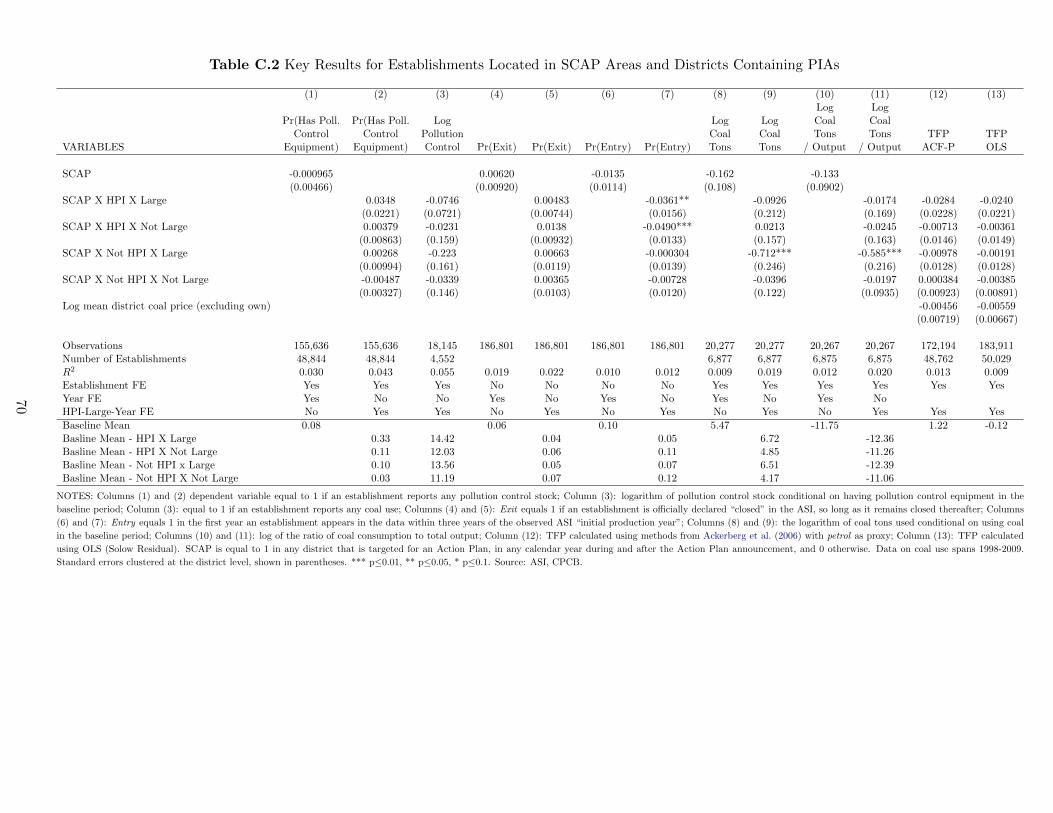
Table C.2 Key Results for Establishments Located in SCAP Areas and Districts Containing PIAs

(1) (2) (3) (4) (5) (6) (7) (8) (9) (10) (11) (12) (13)Log Log

Pr(Has Poll. Pr(Has Poll. Log Log Log Coal CoalControl Control Pollution Coal Coal Tons Tons TFP TFP

VARIABLES Equipment) Equipment) Control Pr(Exit) Pr(Exit) Pr(Entry) Pr(Entry) Tons Tons / Output / Output ACF-P OLS

SCAP -0.000965 0.00620 -0.0135 -0.162 -0.133(0.00466) (0.00920) (0.0114) (0.108) (0.0902)

SCAP X HPI X Large 0.0348 -0.0746 0.00483 -0.0361** -0.0926 -0.0174 -0.0284 -0.0240(0.0221) (0.0721) (0.00744) (0.0156) (0.212) (0.169) (0.0228) (0.0221)

SCAP X HPI X Not Large 0.00379 -0.0231 0.0138 -0.0490*** 0.0213 -0.0245 -0.00713 -0.00361(0.00863) (0.159) (0.00932) (0.0133) (0.157) (0.163) (0.0146) (0.0149)

SCAP X Not HPI X Large 0.00268 -0.223 0.00663 -0.000304 -0.712*** -0.585*** -0.00978 -0.00191(0.00994) (0.161) (0.0119) (0.0139) (0.246) (0.216) (0.0128) (0.0128)

SCAP X Not HPI X Not Large -0.00487 -0.0339 0.00365 -0.00728 -0.0396 -0.0197 0.000384 -0.00385(0.00327) (0.146) (0.0103) (0.0120) (0.122) (0.0935) (0.00923) (0.00891)

Log mean district coal price (excluding own) -0.00456 -0.00559(0.00719) (0.00667)

Observations 155,636 155,636 18,145 186,801 186,801 186,801 186,801 20,277 20,277 20,267 20,267 172,194 183,911Number of Establishments 48,844 48,844 4,552 6,877 6,877 6,875 6,875 48,762 50,029R2 0.030 0.043 0.055 0.019 0.022 0.010 0.012 0.009 0.019 0.012 0.020 0.013 0.009Establishment FE Yes Yes Yes No No No No Yes Yes Yes Yes Yes YesYear FE Yes No No Yes No Yes No Yes No Yes NoHPI-Large-Year FE No Yes Yes No Yes No Yes No Yes No Yes Yes Yes

Baseline Mean 0.08 0.06 0.10 5.47 -11.75 1.22 -0.12Basline Mean - HPI X Large 0.33 14.42 0.04 0.05 6.72 -12.36Basline Mean - HPI X Not Large 0.11 12.03 0.06 0.11 4.85 -11.26Basline Mean - Not HPI x Large 0.10 13.56 0.05 0.07 6.51 -12.39Basline Mean - Not HPI X Not Large 0.03 11.19 0.07 0.12 4.17 -11.06

NOTES: Columns (1) and (2) dependent variable equal to 1 if an establishment reports any pollution control stock; Column (3): logarithm of pollution control stock conditional on having pollution control equipment in the

baseline period; Column (3): equal to 1 if an establishment reports any coal use; Columns (4) and (5): Exit equals 1 if an establishment is officially declared “closed” in the ASI, so long as it remains closed thereafter; Columns

(6) and (7): Entry equals 1 in the first year an establishment appears in the data within three years of the observed ASI “initial production year”; Columns (8) and (9): the logarithm of coal tons used conditional on using coal

in the baseline period; Columns (10) and (11): log of the ratio of coal consumption to total output; Column (12): TFP calculated using methods from Ackerberg et al. (2006) with petrol as proxy; Column (13): TFP calculated

using OLS (Solow Residual). SCAP is equal to 1 in any district that is targeted for an Action Plan, in any calendar year during and after the Action Plan announcement, and 0 otherwise. Data on coal use spans 1998-2009.

Standard errors clustered at the district level, shown in parentheses. *** p≤0.01, ** p≤0.05, * p≤0.1. Source: ASI, CPCB.

70

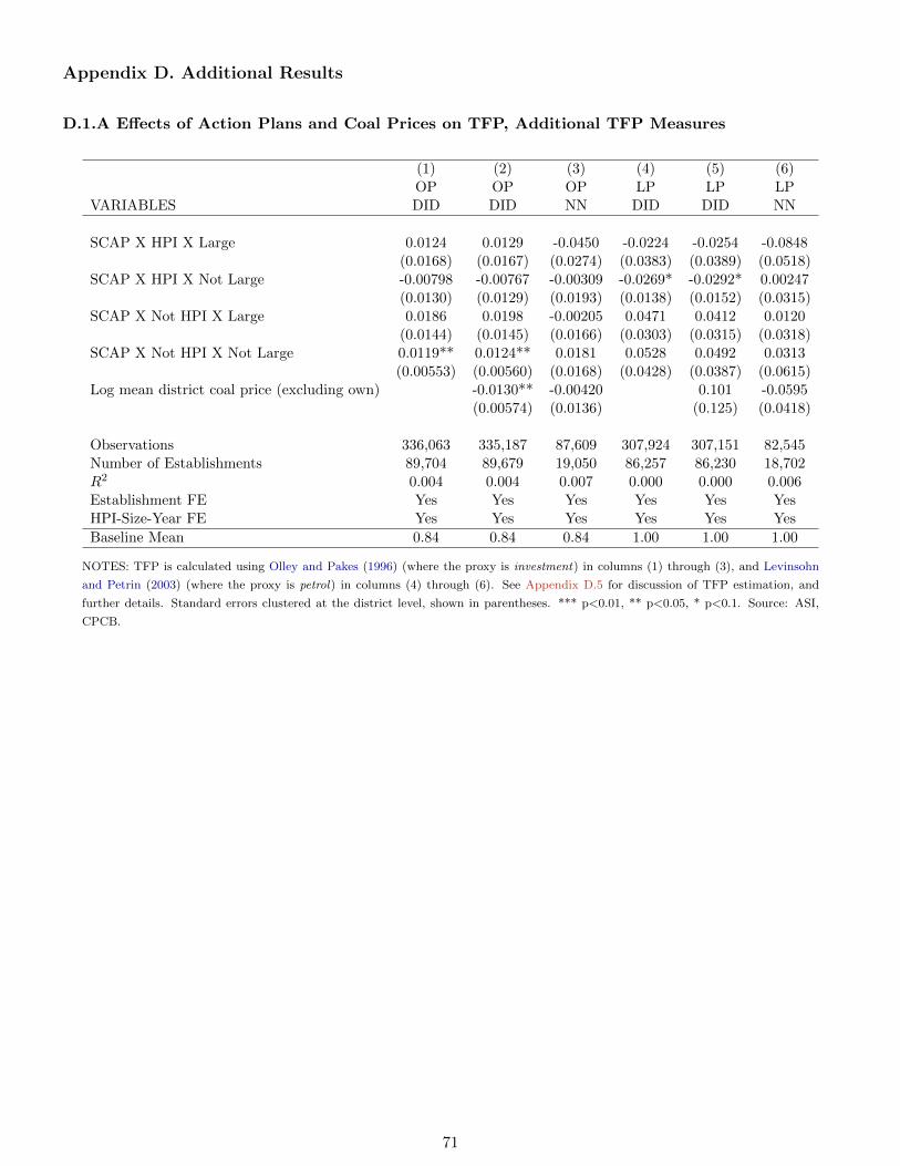
Appendix D. Additional Results

D.1.A Effects of Action Plans and Coal Prices on TFP, Additional TFP Measures

(1) (2) (3) (4) (5) (6)OP OP OP LP LP LP

VARIABLES DID DID NN DID DID NN

SCAP X HPI X Large 0.0124 0.0129 -0.0450 -0.0224 -0.0254 -0.0848(0.0168) (0.0167) (0.0274) (0.0383) (0.0389) (0.0518)

SCAP X HPI X Not Large -0.00798 -0.00767 -0.00309 -0.0269* -0.0292* 0.00247(0.0130) (0.0129) (0.0193) (0.0138) (0.0152) (0.0315)

SCAP X Not HPI X Large 0.0186 0.0198 -0.00205 0.0471 0.0412 0.0120(0.0144) (0.0145) (0.0166) (0.0303) (0.0315) (0.0318)

SCAP X Not HPI X Not Large 0.0119** 0.0124** 0.0181 0.0528 0.0492 0.0313(0.00553) (0.00560) (0.0168) (0.0428) (0.0387) (0.0615)

Log mean district coal price (excluding own) -0.0130** -0.00420 0.101 -0.0595(0.00574) (0.0136) (0.125) (0.0418)

Observations 336,063 335,187 87,609 307,924 307,151 82,545Number of Establishments 89,704 89,679 19,050 86,257 86,230 18,702R2 0.004 0.004 0.007 0.000 0.000 0.006Establishment FE Yes Yes Yes Yes Yes YesHPI-Size-Year FE Yes Yes Yes Yes Yes Yes

Baseline Mean 0.84 0.84 0.84 1.00 1.00 1.00

NOTES: TFP is calculated using Olley and Pakes (1996) (where the proxy is investment) in columns (1) through (3), and Levinsohn

and Petrin (2003) (where the proxy is petrol) in columns (4) through (6). See Appendix D.5 for discussion of TFP estimation, and

further details. Standard errors clustered at the district level, shown in parentheses. *** p<0.01, ** p<0.05, * p<0.1. Source: ASI,

CPCB.

71

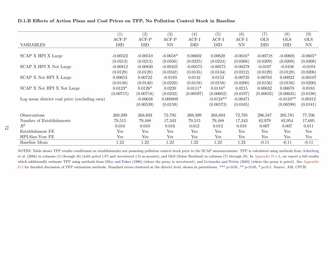
D.1.B Effects of Action Plans and Coal Prices on TFP, No Pollution Control Stock in Baseline

(1) (2) (3) (4) (5) (6) (7) (8) (9)ACF-P ACF-P ACF-P ACF-I ACF-I ACF-I OLS OLS OLS

VARIABLES DID DID NN DID DID NN DID DID NN

SCAP X HPI X Large -0.00522 -0.00510 -0.0658* 0.00602 0.00628 -0.0616* -0.00718 -0.00691 -0.0605*(0.0213) (0.0213) (0.0356) (0.0225) (0.0224) (0.0366) (0.0209) (0.0208) (0.0308)

SCAP X HPI X Not Large -0.00812 -0.00830 -0.00425 -0.00575 -0.00575 -0.00278 -0.0107 -0.0108 -0.0104(0.0128) (0.0128) (0.0242) (0.0135) (0.0134) (0.0212) (0.0129) (0.0128) (0.0206)

SCAP X Not HPI X Large 0.00653 0.00722 -0.0193 0.0142 0.0153 -0.00735 0.00783 0.00922 -0.00107(0.0140) (0.0140) (0.0220) (0.0158) (0.0158) (0.0200) (0.0156) (0.0156) (0.0200)

SCAP X Not HPI X Not Large 0.0123* 0.0126* 0.0220 0.0111* 0.0116* 0.0215 0.00632 0.00678 0.0183(0.00715) (0.00718) (0.0232) (0.00597) (0.00602) (0.0197) (0.00632) (0.00635) (0.0198)

Log mean district coal price (excluding own) -0.00638 0.000888 -0.0124** -0.00471 -0.0133** 0.00312(0.00539) (0.0159) (0.00573) (0.0165) (0.00598) (0.0181)

Observations 269,399 268,693 72,795 269,399 268,693 72,795 296,587 295,781 77,706Number of Establishments 79,515 79,488 17,343 79,515 79,488 17,343 82,979 82,954 17,695R2 0.010 0.010 0.016 0.012 0.012 0.018 0.007 0.007 0.011Establishment FE Yes Yes Yes Yes Yes Yes Yes Yes YesHPI-Size-Year FE Yes Yes Yes Yes Yes Yes Yes Yes Yes

Baseline Mean 1.22 1.22 1.22 1.22 1.22 1.22 -0.11 -0.11 -0.11

NOTES: Table shows TFP results conditional on establishments not possesing pollution control stock prior to the SCAP announcements. TFP is calculated using methods from Ackerberg

et al. (2006) in columns (1) through (6) (with petrol (-P) and investment (-I) as proxies), and OLS (Solow Residual) in columns (7) through (9). In Appendix D.1.A, we report a full results

which additionally estimate TFP using methods from Olley and Pakes (1996) (where the proxy is investment), and Levinsohn and Petrin (2003) (where the proxy is petrol). See Appendix

D.5 for detailed discussion of TFP estimation methods. Standard errors clustered at the district level, shown in parentheses. *** p<0.01, ** p<0.05, * p<0.1. Source: ASI, CPCB.

72

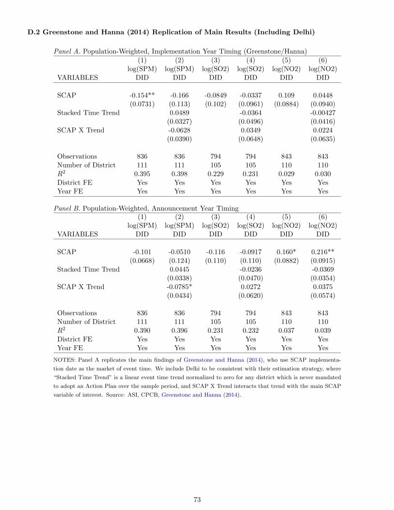
D.2 Greenstone and Hanna (2014) Replication of Main Results (Including Delhi)

Panel A. Population-Weighted, Implementation Year Timing (Greenstone/Hanna)(1) (2) (3) (4) (5) (6)

log(SPM) log(SPM) log(SO2) log(SO2) log(NO2) log(NO2)VARIABLES DID DID DID DID DID DID

SCAP -0.154** -0.166 -0.0849 -0.0337 0.109 0.0448(0.0731) (0.113) (0.102) (0.0961) (0.0884) (0.0940)

Stacked Time Trend 0.0489 -0.0364 -0.00427(0.0327) (0.0496) (0.0416)

SCAP X Trend -0.0628 0.0349 0.0224(0.0390) (0.0648) (0.0635)

Observations 836 836 794 794 843 843Number of District 111 111 105 105 110 110R2 0.395 0.398 0.229 0.231 0.029 0.030District FE Yes Yes Yes Yes Yes YesYear FE Yes Yes Yes Yes Yes Yes

Panel B. Population-Weighted, Announcement Year Timing(1) (2) (3) (4) (5) (6)

log(SPM) log(SPM) log(SO2) log(SO2) log(NO2) log(NO2)VARIABLES DID DID DID DID DID DID

SCAP -0.101 -0.0510 -0.116 -0.0917 0.160* 0.216**(0.0668) (0.124) (0.110) (0.110) (0.0882) (0.0915)

Stacked Time Trend 0.0445 -0.0236 -0.0369(0.0338) (0.0470) (0.0354)

SCAP X Trend -0.0785* 0.0272 0.0375(0.0434) (0.0620) (0.0574)

Observations 836 836 794 794 843 843Number of District 111 111 105 105 110 110R2 0.390 0.396 0.231 0.232 0.037 0.039District FE Yes Yes Yes Yes Yes YesYear FE Yes Yes Yes Yes Yes Yes

NOTES: Panel A replicates the main findings of Greenstone and Hanna (2014), who use SCAP implementa-

tion date as the market of event time. We include Delhi to be consistent with their estimation strategy, where

“Stacked Time Trend” is a linear event time trend normalized to zero for any district which is never mandated

to adopt an Action Plan over the sample period, and SCAP X Trend interacts that trend with the main SCAP

variable of interest. Source: ASI, CPCB, Greenstone and Hanna (2014).

73

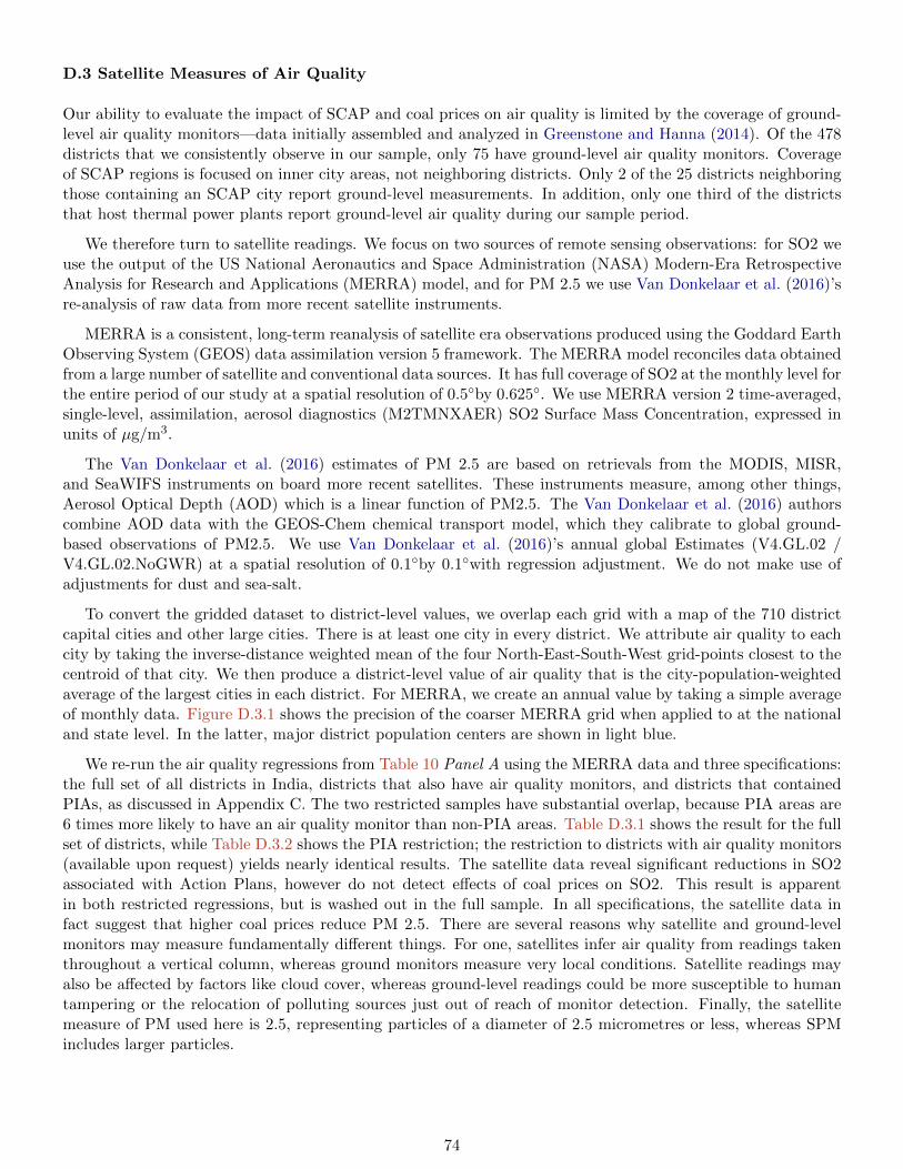
D.3 Satellite Measures of Air Quality

Our ability to evaluate the impact of SCAP and coal prices on air quality is limited by the coverage of ground-level air quality monitors—data initially assembled and analyzed in Greenstone and Hanna (2014). Of the 478districts that we consistently observe in our sample, only 75 have ground-level air quality monitors. Coverageof SCAP regions is focused on inner city areas, not neighboring districts. Only 2 of the 25 districts neighboringthose containing an SCAP city report ground-level measurements. In addition, only one third of the districtsthat host thermal power plants report ground-level air quality during our sample period.

We therefore turn to satellite readings. We focus on two sources of remote sensing observations: for SO2 weuse the output of the US National Aeronautics and Space Administration (NASA) Modern-Era RetrospectiveAnalysis for Research and Applications (MERRA) model, and for PM 2.5 we use Van Donkelaar et al. (2016)’sre-analysis of raw data from more recent satellite instruments.

MERRA is a consistent, long-term reanalysis of satellite era observations produced using the Goddard EarthObserving System (GEOS) data assimilation version 5 framework. The MERRA model reconciles data obtainedfrom a large number of satellite and conventional data sources. It has full coverage of SO2 at the monthly level forthe entire period of our study at a spatial resolution of 0.5◦by 0.625◦. We use MERRA version 2 time-averaged,single-level, assimilation, aerosol diagnostics (M2TMNXAER) SO2 Surface Mass Concentration, expressed inunits of µg/m3.

The Van Donkelaar et al. (2016) estimates of PM 2.5 are based on retrievals from the MODIS, MISR,and SeaWIFS instruments on board more recent satellites. These instruments measure, among other things,Aerosol Optical Depth (AOD) which is a linear function of PM2.5. The Van Donkelaar et al. (2016) authorscombine AOD data with the GEOS-Chem chemical transport model, which they calibrate to global ground-based observations of PM2.5. We use Van Donkelaar et al. (2016)’s annual global Estimates (V4.GL.02 /V4.GL.02.NoGWR) at a spatial resolution of 0.1◦by 0.1◦with regression adjustment. We do not make use ofadjustments for dust and sea-salt.

To convert the gridded dataset to district-level values, we overlap each grid with a map of the 710 districtcapital cities and other large cities. There is at least one city in every district. We attribute air quality to eachcity by taking the inverse-distance weighted mean of the four North-East-South-West grid-points closest to thecentroid of that city. We then produce a district-level value of air quality that is the city-population-weightedaverage of the largest cities in each district. For MERRA, we create an annual value by taking a simple averageof monthly data. Figure D.3.1 shows the precision of the coarser MERRA grid when applied to at the nationaland state level. In the latter, major district population centers are shown in light blue.

We re-run the air quality regressions from Table 10 Panel A using the MERRA data and three specifications:the full set of all districts in India, districts that also have air quality monitors, and districts that containedPIAs, as discussed in Appendix C. The two restricted samples have substantial overlap, because PIA areas are6 times more likely to have an air quality monitor than non-PIA areas. Table D.3.1 shows the result for the fullset of districts, while Table D.3.2 shows the PIA restriction; the restriction to districts with air quality monitors(available upon request) yields nearly identical results. The satellite data reveal significant reductions in SO2associated with Action Plans, however do not detect effects of coal prices on SO2. This result is apparentin both restricted regressions, but is washed out in the full sample. In all specifications, the satellite data infact suggest that higher coal prices reduce PM 2.5. There are several reasons why satellite and ground-levelmonitors may measure fundamentally different things. For one, satellites infer air quality from readings takenthroughout a vertical column, whereas ground monitors measure very local conditions. Satellite readings mayalso be affected by factors like cloud cover, whereas ground-level readings could be more susceptible to humantampering or the relocation of polluting sources just out of reach of monitor detection. Finally, the satellitemeasure of PM used here is 2.5, representing particles of a diameter of 2.5 micrometres or less, whereas SPMincludes larger particles.

74

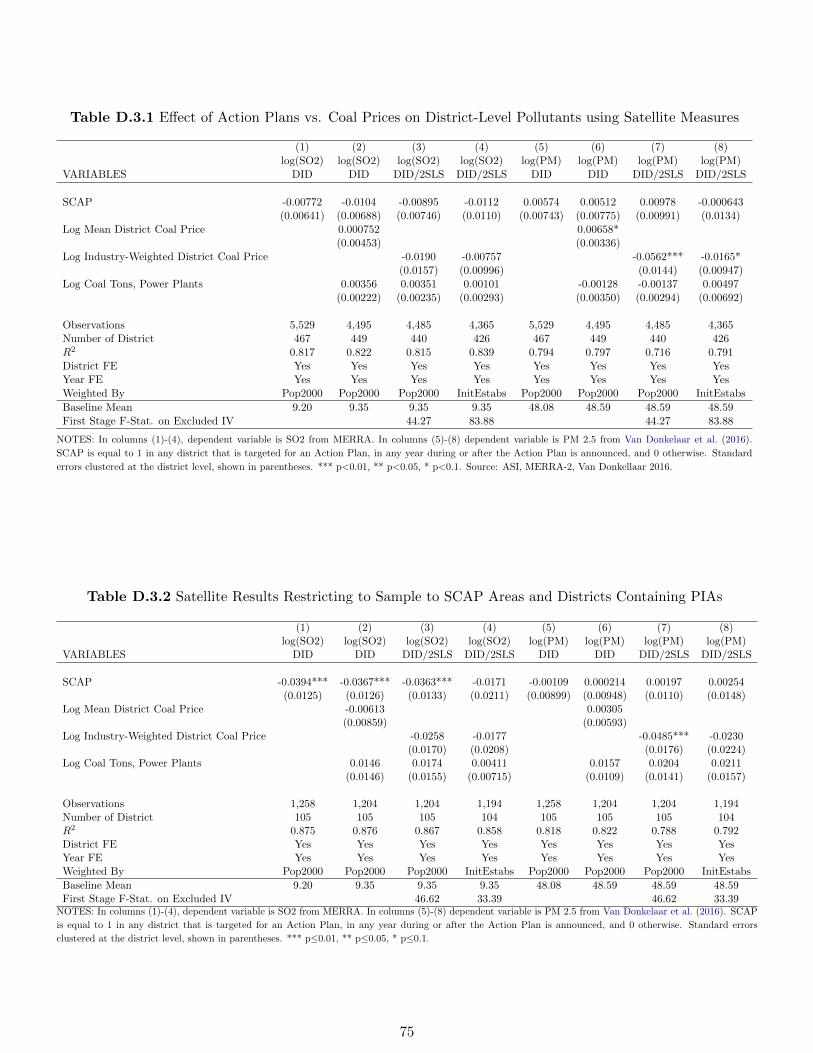
Table D.3.1 Effect of Action Plans vs. Coal Prices on District-Level Pollutants using Satellite Measures

(1) (2) (3) (4) (5) (6) (7) (8)log(SO2) log(SO2) log(SO2) log(SO2) log(PM) log(PM) log(PM) log(PM)

VARIABLES DID DID DID/2SLS DID/2SLS DID DID DID/2SLS DID/2SLS

SCAP -0.00772 -0.0104 -0.00895 -0.0112 0.00574 0.00512 0.00978 -0.000643(0.00641) (0.00688) (0.00746) (0.0110) (0.00743) (0.00775) (0.00991) (0.0134)

Log Mean District Coal Price 0.000752 0.00658*(0.00453) (0.00336)

Log Industry-Weighted District Coal Price -0.0190 -0.00757 -0.0562*** -0.0165*(0.0157) (0.00996) (0.0144) (0.00947)

Log Coal Tons, Power Plants 0.00356 0.00351 0.00101 -0.00128 -0.00137 0.00497(0.00222) (0.00235) (0.00293) (0.00350) (0.00294) (0.00692)

Observations 5,529 4,495 4,485 4,365 5,529 4,495 4,485 4,365Number of District 467 449 440 426 467 449 440 426R2 0.817 0.822 0.815 0.839 0.794 0.797 0.716 0.791District FE Yes Yes Yes Yes Yes Yes Yes YesYear FE Yes Yes Yes Yes Yes Yes Yes YesWeighted By Pop2000 Pop2000 Pop2000 InitEstabs Pop2000 Pop2000 Pop2000 InitEstabs

Baseline Mean 9.20 9.35 9.35 9.35 48.08 48.59 48.59 48.59First Stage F-Stat. on Excluded IV 44.27 83.88 44.27 83.88

NOTES: In columns (1)-(4), dependent variable is SO2 from MERRA. In columns (5)-(8) dependent variable is PM 2.5 from Van Donkelaar et al. (2016).

SCAP is equal to 1 in any district that is targeted for an Action Plan, in any year during or after the Action Plan is announced, and 0 otherwise. Standard

errors clustered at the district level, shown in parentheses. *** p<0.01, ** p<0.05, * p<0.1. Source: ASI, MERRA-2, Van Donkellaar 2016.

Table D.3.2 Satellite Results Restricting to Sample to SCAP Areas and Districts Containing PIAs

(1) (2) (3) (4) (5) (6) (7) (8)log(SO2) log(SO2) log(SO2) log(SO2) log(PM) log(PM) log(PM) log(PM)

VARIABLES DID DID DID/2SLS DID/2SLS DID DID DID/2SLS DID/2SLS

SCAP -0.0394*** -0.0367*** -0.0363*** -0.0171 -0.00109 0.000214 0.00197 0.00254(0.0125) (0.0126) (0.0133) (0.0211) (0.00899) (0.00948) (0.0110) (0.0148)

Log Mean District Coal Price -0.00613 0.00305(0.00859) (0.00593)

Log Industry-Weighted District Coal Price -0.0258 -0.0177 -0.0485*** -0.0230(0.0170) (0.0208) (0.0176) (0.0224)

Log Coal Tons, Power Plants 0.0146 0.0174 0.00411 0.0157 0.0204 0.0211(0.0146) (0.0155) (0.00715) (0.0109) (0.0141) (0.0157)

Observations 1,258 1,204 1,204 1,194 1,258 1,204 1,204 1,194Number of District 105 105 105 104 105 105 105 104R2 0.875 0.876 0.867 0.858 0.818 0.822 0.788 0.792District FE Yes Yes Yes Yes Yes Yes Yes YesYear FE Yes Yes Yes Yes Yes Yes Yes YesWeighted By Pop2000 Pop2000 Pop2000 InitEstabs Pop2000 Pop2000 Pop2000 InitEstabs

Baseline Mean 9.20 9.35 9.35 9.35 48.08 48.59 48.59 48.59First Stage F-Stat. on Excluded IV 46.62 33.39 46.62 33.39

NOTES: In columns (1)-(4), dependent variable is SO2 from MERRA. In columns (5)-(8) dependent variable is PM 2.5 from Van Donkelaar et al. (2016). SCAP

is equal to 1 in any district that is targeted for an Action Plan, in any year during or after the Action Plan is announced, and 0 otherwise. Standard errors

clustered at the district level, shown in parentheses. *** p≤0.01, ** p≤0.05, * p≤0.1.

75

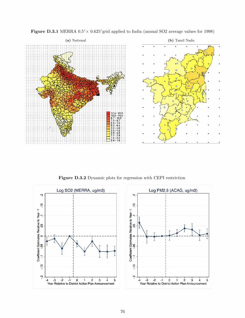
Figure D.3.1 MERRA 0.5◦× 0.625◦grid applied to India (annual SO2 average values for 1998)

(a) National (b) Tamil Nadu

Figure D.3.2 Dynamic plots for regression with CEPI restriction

76

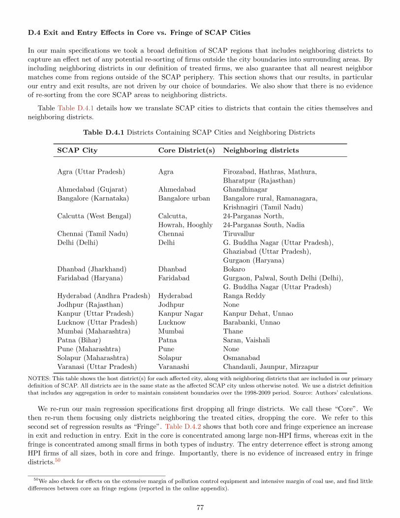
D.4 Exit and Entry Effects in Core vs. Fringe of SCAP Cities

In our main specifications we took a broad definition of SCAP regions that includes neighboring districts tocapture an effect net of any potential re-sorting of firms outside the city boundaries into surrounding areas. Byincluding neighboring districts in our definition of treated firms, we also guarantee that all nearest neighbormatches come from regions outside of the SCAP periphery. This section shows that our results, in particularour entry and exit results, are not driven by our choice of boundaries. We also show that there is no evidenceof re-sorting from the core SCAP areas to neighboring districts.

Table Table D.4.1 details how we translate SCAP cities to districts that contain the cities themselves andneighboring districts.

Table D.4.1 Districts Containing SCAP Cities and Neighboring Districts

SCAP City Core District(s) Neighboring districts

Agra (Uttar Pradesh) Agra Firozabad, Hathras, Mathura,Bharatpur (Rajasthan)

Ahmedabad (Gujarat) Ahmedabad GhandhinagarBangalore (Karnataka) Bangalore urban Bangalore rural, Ramanagara,

Krishnagiri (Tamil Nadu)Calcutta (West Bengal) Calcutta, 24-Parganas North,

Howrah, Hooghly 24-Parganas South, NadiaChennai (Tamil Nadu) Chennai TiruvallurDelhi (Delhi) Delhi G. Buddha Nagar (Uttar Pradesh),

Ghaziabad (Uttar Pradesh),Gurgaon (Haryana)

Dhanbad (Jharkhand) Dhanbad BokaroFaridabad (Haryana) Faridabad Gurgaon, Palwal, South Delhi (Delhi),

G. Buddha Nagar (Uttar Pradesh)Hyderabad (Andhra Pradesh) Hyderabad Ranga ReddyJodhpur (Rajasthan) Jodhpur NoneKanpur (Uttar Pradesh) Kanpur Nagar Kanpur Dehat, UnnaoLucknow (Uttar Pradesh) Lucknow Barabanki, UnnaoMumbai (Maharashtra) Mumbai ThanePatna (Bihar) Patna Saran, VaishaliPune (Maharashtra) Pune NoneSolapur (Maharashtra) Solapur OsmanabadVaranasi (Uttar Pradesh) Varanashi Chandauli, Jaunpur, Mirzapur

NOTES: This table shows the host district(s) for each affected city, along with neighboring districts that are included in our primarydefinition of SCAP. All districts are in the same state as the affected SCAP city unless otherwise noted. We use a district definitionthat includes any aggregation in order to maintain consistent boundaries over the 1998-2009 period. Source: Authors’ calculations.

We re-run our main regression specifications first dropping all fringe districts. We call these “Core”. Wethen re-run them focusing only districts neighboring the treated cities, dropping the core. We refer to thissecond set of regression results as “Fringe”. Table D.4.2 shows that both core and fringe experience an increasein exit and reduction in entry. Exit in the core is concentrated among large non-HPI firms, whereas exit in thefringe is concentrated among small firms in both types of industry. The entry deterrence effect is strong amongHPI firms of all sizes, both in core and fringe. Importantly, there is no evidence of increased entry in fringedistricts.50

50We also check for effects on the extensive margin of pollution control equipment and intensive margin of coal use, and find littledifferences between core an fringe regions (reported in the online appendix).

77

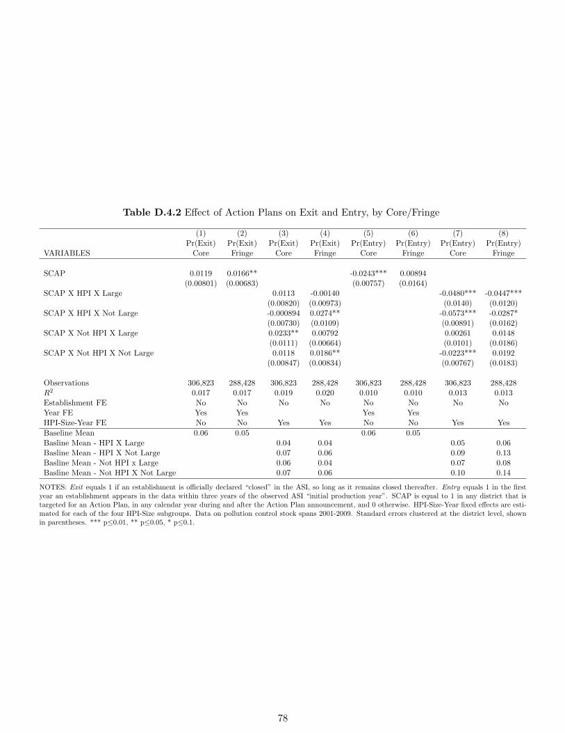
Table D.4.2 Effect of Action Plans on Exit and Entry, by Core/Fringe

(1) (2) (3) (4) (5) (6) (7) (8)Pr(Exit) Pr(Exit) Pr(Exit) Pr(Exit) Pr(Entry) Pr(Entry) Pr(Entry) Pr(Entry)

VARIABLES Core Fringe Core Fringe Core Fringe Core Fringe

SCAP 0.0119 0.0166** -0.0243*** 0.00894(0.00801) (0.00683) (0.00757) (0.0164)

SCAP X HPI X Large 0.0113 -0.00140 -0.0480*** -0.0447***(0.00820) (0.00973) (0.0140) (0.0120)

SCAP X HPI X Not Large -0.000894 0.0274** -0.0573*** -0.0287*(0.00730) (0.0109) (0.00891) (0.0162)

SCAP X Not HPI X Large 0.0233** 0.00792 0.00261 0.0148(0.0111) (0.00664) (0.0101) (0.0186)

SCAP X Not HPI X Not Large 0.0118 0.0186** -0.0223*** 0.0192(0.00847) (0.00834) (0.00767) (0.0183)

Observations 306,823 288,428 306,823 288,428 306,823 288,428 306,823 288,428R2 0.017 0.017 0.019 0.020 0.010 0.010 0.013 0.013Establishment FE No No No No No No No NoYear FE Yes Yes Yes YesHPI-Size-Year FE No No Yes Yes No No Yes Yes

Baseline Mean 0.06 0.05 0.06 0.05Basline Mean - HPI X Large 0.04 0.04 0.05 0.06Basline Mean - HPI X Not Large 0.07 0.06 0.09 0.13Basline Mean - Not HPI x Large 0.06 0.04 0.07 0.08Basline Mean - Not HPI X Not Large 0.07 0.06 0.10 0.14

NOTES: Exit equals 1 if an establishment is officially declared “closed” in the ASI, so long as it remains closed thereafter. Entry equals 1 in the firstyear an establishment appears in the data within three years of the observed ASI “initial production year”. SCAP is equal to 1 in any district that istargeted for an Action Plan, in any calendar year during and after the Action Plan announcement, and 0 otherwise. HPI-Size-Year fixed effects are esti-mated for each of the four HPI-Size subgroups. Data on pollution control stock spans 2001-2009. Standard errors clustered at the district level, shownin parentheses. *** p≤0.01, ** p≤0.05, * p≤0.1.

78

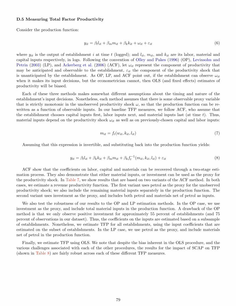
D.5 Measuring Total Factor Productivity

Consider the production function:

yit = βllit + βmmit + βkkit + ωit + εit (6)

where yit is the output of establishment i at time t (logged); and lit, mit, and kit are its labor, material andcapital inputs respectively, in logs. Following the convention of Olley and Pakes (1996) (OP), Levinsohn andPetrin (2003) (LP), and Ackerberg et al. (2006) (ACF), let ωit represent the component of productivity thatmay be anticipated and observable to the establishment, εit the component of the productivity shock thatis unanticipated by the establishment. As OP, LP, and ACF point out, if the establishment can observe ωitwhen it makes its input decisions, but the econometrician cannot, then OLS (and fixed effects) estimates ofproductivity will be biased.

Each of these three methods makes somewhat different assumptions about the timing and nature of theestablishment’s input decisions. Nonetheless, each method assumes that there is some observable proxy variablethat is strictly monotonic in the unobserved productivity shock ω, so that the production function can be re-written as a function of observable inputs. In our baseline TFP measures, we follow ACF, who assume thatthe establishment chooses capital inputs first, labor inputs next, and material inputs last (at time t). Thus,material inputs depend on the productivity shock ωit as well as on previously-chosen capital and labor inputs:

mit = ft(wit, kit, lit) (7)

Assuming that this expression is invertible, and substituting back into the production function yields:

yit = βllit + βkkit + βmmit + βkf−1t (mit, kit, lit) + εit (8)

ACF show that the coefficients on labor, capital and materials can be recovered through a two-stage esti-mation process. They also demonstrate that either material inputs, or investment can be used as the proxy forthe productivity shock. In Table 7, we show results that are based on two variants of the ACF method. In bothcases, we estimate a revenue productivity function. The first variant uses petrol as the proxy for the unobservedproductivity shock; we also include the remaining material inputs separately in the production function. Thesecond variant uses investment as the proxy, and includes both petrol and materials net of petrol as inputs.

We also test the robustness of our results to the OP and LP estimation methods. In the OP case, we useinvestment as the proxy, and include total material inputs in the production function. A drawback of the OPmethod is that we only observe positive investment for approximately 55 percent of establishments (and 75percent of observations in our dataset). Thus, the coefficients on the inputs are estimated based on a subsampleof establishments. Nonetheless, we estimate TFP for all establishments, using the input coefficients that areestimated on the subset of establishments. In the LP case, we use petrol as the proxy, and include materialsnet of petrol in the production function.

Finally, we estimate TFP using OLS. We note that despite the bias inherent in the OLS procedure, and thevarious challenges associated with each of the other procedures, the results for the impact of SCAP on TFP(shown in Table 8) are fairly robust across each of these different TFP measures.

79

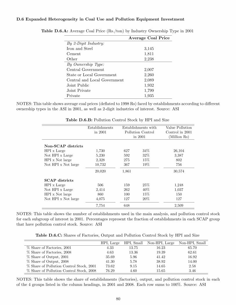
D.6 Expanded Heterogeneity in Coal Use and Pollution Equipment Investment

Table D.6.A: Average Coal Price (Rs./ton) by Industry Ownership Type in 2001

Average Coal Price

By 2-Digit Industry:Iron and Steel 3,145Cement 1,811Other 2,238

By Ownership Type:Central Government 2,007State or Local Government 2,260Central and Local Government 2,089Joint Public 1,932Joint Private 1,799Private 1,935

NOTES: This table shows average coal prices (deflated to 1998 Rs) faced by establishments according to differentownership types in the ASI in 2001, as well as 2-digit industries of interest. Source: ASI

Table D.6.B: Pollution Control Stock by HPI and Size

Establishments Establishments with Value Pollutionin 2001 Pollution Control Control in 2001

in 2001 (Million Rs)

Non-SCAP districtsHPI x Large 1,730 627 34% 26,104Not HPI x Large 5,230 592 32% 3,387HPI x Not large 2,328 275 15% 802Not HPI x Not large 10,732 367 19% 756

20,020 1,861 30,574

SCAP districtsHPI x Large 506 159 25% 1,248Not HPI x Large 2,414 262 40% 1,037HPI x Not large 860 100 15% 150Not HPI x Not large 4,075 127 20% 127

7,754 648 2,509

NOTES: This table shows the number of establishments used in the main analysis, and pollution control stockfor each subgroup of interest in 2001. Percentages represent the fraction of establishments in each SCAP groupthat have pollution control stock. Source: ASI

Table D.6.C: Shares of Factories, Output and Pollution Control Stock by HPI and Size

HPI, Large HPI, Small Non-HPI, Large Non-HPI, Small% Share of Factories, 2001 4.33 13.75 16.23 65.70% Share of Factories, 2008 4.63 13.36 19.39 62.61% Share of Output, 2001 35.69 5.96 41.42 16.92% Share of Output, 2008 41.30 5.78 38.92 14.00% Share of Pollution Control Stock, 2001 73.62 9.15 14.65 2.58% Share of Pollution Control Stock, 2008 76.29 4.60 15.65 3.46

NOTES: This table shows the share of establishments (factories), output, and pollution control stock in eachof the 4 groups listed in the column headings, in 2001 and 2008. Each row sums to 100%. Source: ASI

80

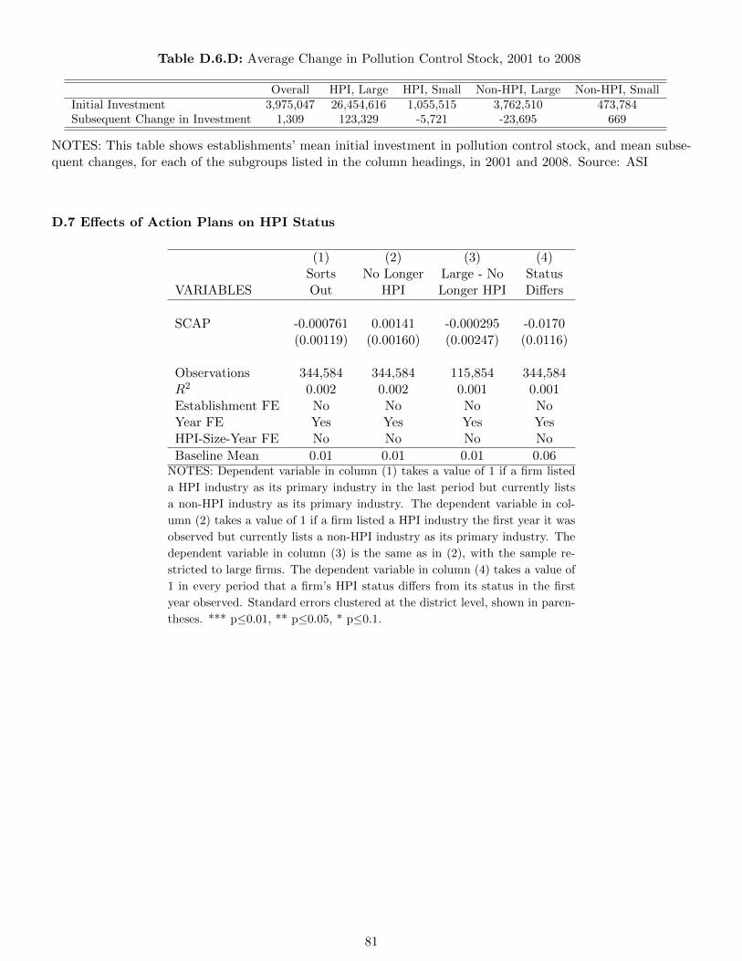
Table D.6.D: Average Change in Pollution Control Stock, 2001 to 2008

Overall HPI, Large HPI, Small Non-HPI, Large Non-HPI, SmallInitial Investment 3,975,047 26,454,616 1,055,515 3,762,510 473,784Subsequent Change in Investment 1,309 123,329 -5,721 -23,695 669

NOTES: This table shows establishments’ mean initial investment in pollution control stock, and mean subse-quent changes, for each of the subgroups listed in the column headings, in 2001 and 2008. Source: ASI

D.7 Effects of Action Plans on HPI Status

(1) (2) (3) (4)Sorts No Longer Large - No Status

VARIABLES Out HPI Longer HPI Differs

SCAP -0.000761 0.00141 -0.000295 -0.0170(0.00119) (0.00160) (0.00247) (0.0116)

Observations 344,584 344,584 115,854 344,584R2 0.002 0.002 0.001 0.001Establishment FE No No No NoYear FE Yes Yes Yes YesHPI-Size-Year FE No No No No

Baseline Mean 0.01 0.01 0.01 0.06NOTES: Dependent variable in column (1) takes a value of 1 if a firm listed

a HPI industry as its primary industry in the last period but currently lists

a non-HPI industry as its primary industry. The dependent variable in col-

umn (2) takes a value of 1 if a firm listed a HPI industry the first year it was

observed but currently lists a non-HPI industry as its primary industry. The

dependent variable in column (3) is the same as in (2), with the sample re-

stricted to large firms. The dependent variable in column (4) takes a value of

1 in every period that a firm’s HPI status differs from its status in the first

year observed. Standard errors clustered at the district level, shown in paren-

theses. *** p≤0.01, ** p≤0.05, * p≤0.1.

81

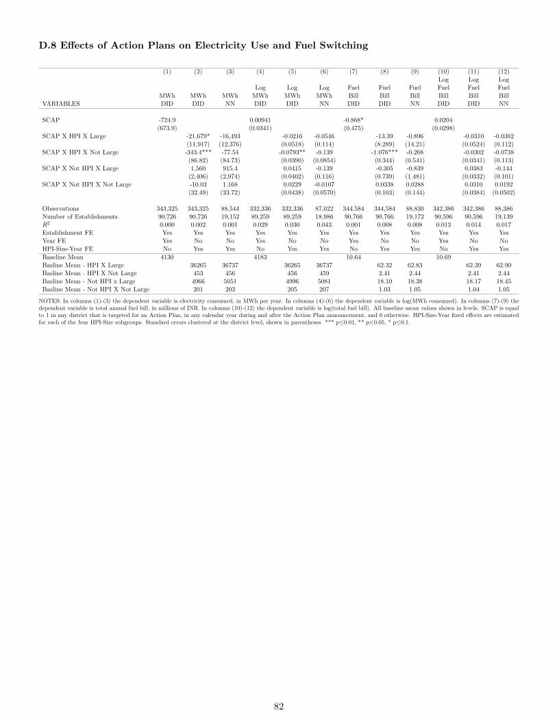
D.8 Effects of Action Plans on Electricity Use and Fuel Switching

(1) (2) (3) (4) (5) (6) (7) (8) (9) (10) (11) (12)Log Log Log

Log Log Log Fuel Fuel Fuel Fuel Fuel FuelMWh MWh MWh MWh MWh MWh Bill Bill Bill Bill Bill Bill

VARIABLES DID DID NN DID DID NN DID DID NN DID DID NN

SCAP -724.9 0.00941 -0.868* 0.0204(673.9) (0.0341) (0.475) (0.0298)

SCAP X HPI X Large -21,679* -16,493 -0.0216 -0.0546 -13.39 -0.896 -0.0310 -0.0382(11,917) (12,376) (0.0518) (0.114) (8.289) (14.21) (0.0524) (0.112)

SCAP X HPI X Not Large -343.4*** -77.54 -0.0793** -0.139 -1.076*** -0.268 -0.0302 -0.0738(86.82) (84.73) (0.0390) (0.0854) (0.344) (0.541) (0.0341) (0.113)

SCAP X Not HPI X Large 1,560 915.4 0.0415 -0.139 -0.305 -0.839 0.0383 -0.144(2,406) (2,974) (0.0402) (0.116) (0.739) (1.481) (0.0332) (0.101)

SCAP X Not HPI X Not Large -10.03 1.168 0.0229 -0.0107 0.0338 0.0288 0.0310 0.0192(32.49) (33.72) (0.0438) (0.0570) (0.103) (0.144) (0.0384) (0.0502)

Observations 343,325 343,325 88,544 332,336 332,336 87,022 344,584 344,584 88,830 342,386 342,386 88,386Number of Establishments 90,726 90,726 19,152 89,259 89,259 18,986 90,766 90,766 19,172 90,596 90,596 19,139R2 0.000 0.002 0.001 0.029 0.030 0.043 0.001 0.008 0.008 0.013 0.014 0.017Establishment FE Yes Yes Yes Yes Yes Yes Yes Yes Yes Yes Yes YesYear FE Yes No No Yes No No Yes No No Yes No NoHPI-Size-Year FE No Yes Yes No Yes Yes No Yes Yes No Yes Yes

Baseline Mean 4130 4183 10.64 10.69Basline Mean - HPI X Large 36265 36737 36265 36737 62.32 62.83 62.39 62.90Basline Mean - HPI X Not Large 453 456 456 459 2.41 2.44 2.41 2.44Basline Mean - Not HPI x Large 4966 5051 4996 5081 18.10 18.38 18.17 18.45Basline Mean - Not HPI X Not Large 201 203 205 207 1.03 1.05 1.04 1.05

NOTES: In columns (1)-(3) the dependent variable is electricity consumed, in MWh per year. In columns (4)-(6) the dependent variable is log(MWh consumed). In columns (7)-(9) thedependent variable is total annual fuel bill, in millions of INR. In columns (10)-(12) the dependent variable is log(total fuel bill). All baseline mean values shown in levels. SCAP is equalto 1 in any district that is targeted for an Action Plan, in any calendar year during and after the Action Plan announcement, and 0 otherwise. HPI-Size-Year fixed effects are estimatedfor each of the four HPI-Size subgroups. Standard errors clustered at the district level, shown in parentheses. *** p≤0.01, ** p≤0.05, * p≤0.1.

82