NBER WORKING PAPER SERIES THE PERFORMANCE OF PERFORMANCE STANDARDS James J. Heckman Carolyn Heinrich Jeffrey Smith Working Paper 9002 http://www.nber.org/papers/w9002 NATIONAL BUREAU OF ECONOMIC RESEARCH 1050 Massachusetts Avenue Cambridge, MA 02138 June 2002 Heckman is Henry Schultz Distinguished Service Professor of Economics at the University of Chicago and a Senior Fellow of the American Bar Foundation. Heinrich is Assistant Professor of Public Policy at the University of North Carolina, Chapel Hill. Smith is an Associate Professor of Economics at the University of Maryland. This research was supported by grants from the American Bar Foundation, the National Science Foundation (SBR-93-4115), the Russell Sage Foundation, the Social Science and Humanities Research Council of Canada and the W.E. Upjohn Institute for Employment Research. We thank Karen Conneely, Miana Plesca, Carla VanBeselaere and Alex Whalley for excellent research assistance. We thank Eric Hanushek for helpful comments. This essay is based in part on research reported in a forthcoming monograph, Heckman (2003). The data used in this article can be obtained beginning Spring, 2003 through Spring, 2006 from Jeffrey Smith, Department of Economics, University of Maryland, 3105 Tydings Hall, College Park, MD 20742. The views expressed herein are those of the authors and not necessarily those of the National Bureau of Economic Research. © 2002 by James J. Heckman, Carolyn Heinrich and Jeffrey Smith. All rights reserved. Short sections of text, not to exceed two paragraphs, may be quoted without explicit permission provided that full credit, including © notice, is given to the source.

Welcome message from author
This document is posted to help you gain knowledge. Please leave a comment to let me know what you think about it! Share it to your friends and learn new things together.
Transcript
NBER WORKING PAPER SERIES
THE PERFORMANCE OF PERFORMANCE STANDARDS
James J. Heckman
Carolyn Heinrich
Jeffrey Smith
Working Paper 9002
http://www.nber.org/papers/w9002
NATIONAL BUREAU OF ECONOMIC RESEARCH
1050 Massachusetts Avenue
Cambridge, MA 02138
June 2002
Heckman is Henry Schultz Distinguished Service Professor of Economics at the University of Chicago and
a Senior Fellow of the American Bar Foundation. Heinrich is Assistant Professor of Public Policy at the
University of North Carolina, Chapel Hill. Smith is an Associate Professor of Economics at the University
of Maryland. This research was supported by grants from the American Bar Foundation, the National Science
Foundation (SBR-93-4115), the Russell Sage Foundation, the Social Science and Humanities Research
Council of Canada and the W.E. Upjohn Institute for Employment Research. We thank Karen Conneely,
Miana Plesca, Carla VanBeselaere and Alex Whalley for excellent research assistance. We thank Eric
Hanushek for helpful comments. This essay is based in part on research reported in a forthcoming
monograph, Heckman (2003). The data used in this article can be obtained beginning Spring, 2003 through
Spring, 2006 from Jeffrey Smith, Department of Economics, University of Maryland, 3105 Tydings Hall,
College Park, MD 20742. The views expressed herein are those of the authors and not necessarily those of
the National Bureau of Economic Research.
© 2002 by James J. Heckman, Carolyn Heinrich and Jeffrey Smith. All rights reserved. Short sections of
text, not to exceed two paragraphs, may be quoted without explicit permission provided that full credit,
including © notice, is given to the source.
The Performance of Performance Standards
James J. Heckman, Carolyn Heinrich and Jeffrey Smith
NBER Working Paper No. 9002
June 2002
JEL No. C31
ABSTRACT
This paper examines the performance of the JTPA performance system, a widely emulated model
for inducing efficiency in government organizations. We present a model of how performance incentives
may distort bureaucratic decisions. We define cream skimming within the model. Two major empirical
findings are (a) that the short run measures used to monitor performance are weakly, and sometimes
perversely, related to long run impacts and (b) that the efficiency gains or losses from cream skimming
are small. We find evidence that centers respond to performance standards.
James Heckman Carolyn Heinrich Jeffrey Smith
Department of Economics Department of Public Policy Department of Economics
University of Chicago University of North Carolina University of Maryland
1126 East 59th Street Abernethy Hall, CB#3435 3105 Tydings Hall
Chicago, IL 60637 Chapel Hill, NC 27599-3435 College Park, MD 20742-7211
and NBER [email protected] and NBER
Heckman, Heinrich, and Smith 2
I. Introduction
Incentives based on performance standards have been advocated to promote productivity
and to direct activity in public organizations. Little is known about how performance standards
systems perform1. This paper presents evidence on this question using data from a social
experiment on a major U.S. government training program with performance standard incentives.
The performance standards system in this program, the Job Training Partnership Act (JTPA), is a
prototype for other government programs. The 1993 Performance Standards Act (U.S. Congress,
1993) required the use of performance systems similar to that of JTPA in many other
government programs. In particular, JTPA's successor as the primary federal training program
for the disadvantaged, the Workforce Investment Act (WIA), utilizes an expanded version of the
JTPA performance system. Performance systems like that in JTPA are in use around the world.
The JTPA incentive system was unique in providing incentives at the local organization
level but not to specific individuals within organizations. Little is known about how
performance standard systems at the level of local organizations work in practice. This paper
presents new evidence on this issue and summarizes related research scattered throughout the
published literature and in government reports. We take it as given that performance standards
affect the behavior of the organization (see, for example, Courty and Marschke, 1996, 1997). In
that light, we address two basic questions. First, do the behavioral responses further the goals of
the program? If not, what do they do instead? Second, how do specific actors within
bureaucracies respond to the incentives presented to them?
The main focus of this paper is on the first question. We consider whether JTPA
performance incentives promoted “desirable” outcomes. Unlike many government programs, the
JTPA program had tangible outputs: the employment and earnings of its participants. There is

Heckman, Heinrich, and Smith 3
widespread agreement that maximizing the gain (for example, the increase in the present value of
discounted earnings relative to what participants would have experienced had they not
participated) is a worthy goal. In addition, the JTPA program was created with clearly stated
objectives, so that there is a well-defined set of targets against which to measure performance.
As noted by Wilson (1989), both features of the JTPA program are unusual when compared to
the many other government agencies that lack clearly stated objectives or adequate
measurements of performance.
Even though the goals of the program are clearly stated, they may be in conflict. The Job
Training Partnership Act (Public Law 97- 300) mandated the provision of employment and
training opportunities to “those who can benefit from, and are most in need of, such
opportunities.” (Section 141 (c)). Since benefit and need are different things, the potential for
conflict between efficiency and equity is written into the law authorizing the program.2 Whether
or not those who benefit most are also the most in need is an empirical question that we
investigate in this paper.
The JTPA program was designed to improve the human capital of its participants.
Evaluation of human capital projects inherently involves evaluation of earnings and employment
trajectories over time, and comparing them to other human capital investments, including no
investment at all. This involves two distinct problems: (a) construction of counterfactual states
(what participants would have earned in their next best alternative) and (b) measuring outcomes
and creating counterfactuals over the harvest period of the investment, which may be a lifetime.
Both problems are difficult. Constructing counterfactual states is a controversial activity (see, for
example, Heckman, 2001, and Heckman, LaLonde, and Smith, 1999). Tracking persons over
time is a costly activity and does not produce short run feedback on the success of the program.
Heckman, Heinrich, and Smith 4
The JTPA performance standards system, and most related systems, attempt to circumvent these
fundamental problems by using the outcomes of participants measured at the time they complete
the program, or within a few months thereafter. Such measures are necessarily short run in
nature. In addition, such systems do not attempt to construct even the short run counterfactual.
Use of these short term outcome measures creates the possibility that the performance
standards misdirect activity by focusing training center attention on criteria that may be
perversely related to long run net benefits, long run equity criteria, or both. This is especially
likely in the context of a human capital program. One benefit of training is that it encourages
further training and schooling. Such additional investment depresses measured employment and
earnings in the short run, but raises it in the long run.3 In this case, the short run measurements
on which performance standards are based will likely be perversely related to long run benefits.
We present evidence on this question and summarize other evidence from the literature. We
establish that fears of misalignment or perverse alignment of the incentives are justified.
Most discussions of performance standards (see, for example, Anderson et al., 1992, and
Barnow, 1992) focus on “cream skimming”. Sometimes this term is defined as selecting persons
into the program who would have done well without it. In the context of a system of
performance standards, cream skimming is defined as selecting people who help attain short run
goals, rather than selecting persons on the basis of their expected long run benefit from
participation. In the current literature, the definition of cream skimming is vague and the
methods used to measure it are not convincing. Implicit in the current literature is the assumption
that program and no-program outcomes are basically the same, except for a positive treatment
effect common to all persons. One contribution of this paper is to precisely define the concept of
cream skimming in the modern language of counterfactuals and to relate it to an economic model

Heckman, Heinrich, and Smith 5
of performance standards. Cream skimming may or may not be a serious problem. If persons
who would have done well without the program have the largest gains from it, then cream
skimming may promote efficiency. We present evidence on this question below.
The paper proceeds as follows. Section II outlines the basic evaluation problem and how
performance standards attempt to solve it. We present a model of training center performance
under performance standards and define cream skimming in the context of our model. Section
III describes the JTPA program and its performance standards system. We show that features of
the JTPA system are in widespread use, so our analysis of JTPA has some generality. Section IV
describes our data. Section V presents evidence on the efficiency effects of cream skimming.
Section VI presents evidence on the effects of performance standards on the behavior of training
centers and their staff. Section VII presents evidence on how well the short run target outcomes
used in performance standards predict long run impacts. Section VIII concludes.
II. Policy Counterfactuals, Performance Standards, and Cream Skimming
A. A Model of Training Center Choices
Successful human capital investment programs produce a time series of returns after the
intervention. For simplicity we analyze a program that takes one period to train persons selected
from the eligible population. Training centers face a new cohort of eligible applicants each
period. All persons in each prospective training cohort have one chance to train. They are then
replaced by the next period’s cohort. The environment is assumed to be stationary so that the
same decision rules are followed each period given the same state variables (that is, the
environment facing the center). There is a benchmark outcome that corresponds to no program
or the next best program. Persons participate or not in period “0” of their lifecycle. Thus, we
Heckman, Heinrich, and Smith 6
normalize lifecycle periods relative to the benchmark period when the training participation
decision is made.4 Participants experience a series of outcomes, 1, 0, ,
aY a A= K where A is the
final period of the person's life. In the absence of the program, persons experience outcomes
0, 0, ,
aY a A= K . The per-period treatment effect is 1 0
a a aY Y− = ∆ . The treatment effect can be
negative in the short run if the initial investment leads to additional investment.5 To make our
analysis fit into a standard cost-benefit framework, let Y denote earnings. Given direct cost, c,
and discount rate r, the net present value of the program impacts measured at time zero is
(1) ( )0 1
A
a
a
a
c PV
r=
∆ − =+
∑
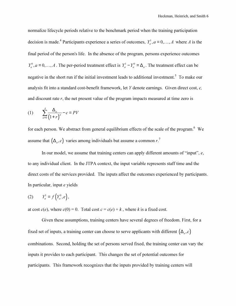
for each person. We abstract from general equilibrium effects of the scale of the program.6 We
assume that ( ),ac∆ varies among individuals but assume a common r.7
In our model, we assume that training centers can apply different amounts of “input”, e,
to any individual client. In the JTPA context, the input variable represents staff time and the
direct costs of the services provided. The inputs affect the outcomes experienced by participants.
In particular, input e yields
(2) ( )1 0,
a aY f Y e= ,
at cost c(e), where c(0) = 0. Total cost c = c(e) + k , where k is a fixed cost.
Given these assumptions, training centers have several degrees of freedom. First, for a
fixed set of inputs, a training center can choose to serve applicants with different ( ),ac∆
combinations. Second, holding the set of persons served fixed, the training center can vary the
inputs it provides to each participant. This changes the set of potential outcomes for
participants. This framework recognizes that the inputs provided by training centers will

Heckman, Heinrich, and Smith 7
augment or reduce the potential outcome that participants would have experienced in the absence
of participation. Third, a training center can choose how many participants to serve by trading
off between the fixed per participant costs k and the variable per participant input costs c(e).
If the goal of the training center is to maximize the ex post present value of the earnings
impacts realized by its trainees, it solves a constrained optimization problem that we now
describe. Notice that if there were no budget constraints, the center would find the e that
maximizes the present value of the earnings impacts for each participant:
(3) ( )
( )1 0
0
( )ˆ argmax .
1
A
a a
ae a
Y Ye c e k
r=
−= − −+
∑
Training centers operate under a budget constraint B. Thus they face a tradeoff between
serving more clients and increasing inputs per client. Let {1,…,I} be the index set of eligible
applicants. Person i has an associated cost (variable, ci(e), and fixed, ki.). We assume that
technology (2) is common across persons although this assumption can easily be relaxed.
Associated with each potential set of trainees, { }1,...,S I⊂ is a number of trainees N(S). For each
cohort, the center solves the problem
(4) ( )
( )( )
i
1 0
, ,
,0
Max ,1
Aa i a i
i i iae i S
i S a
Y Yc e k
r∈ ∈ =
− − − +
∑ ∑
subject to (2) and
(5) ( )( )∑∈
+≥Si
iiikecB .
For LaGrange multiplier λ attached to (5), this produces the first order condition for each
observation ,Si ∈

Heckman, Heinrich, and Smith 8
(6) ( )
( )( )0
,
0
, 1.
1
Ai a i i i
a
a i i
f Y e c e
e erλ
=
∂ ∂ = ∂ ∂+
∑
This is the standard efficiency condition for ei (marginal benefit equals marginal cost). In the
absence of a budget constraint, λ = 1 at an interior optimum. In general, λ ≥ 1, reflecting the
scarcity of the resources available to the center, and the center invests less in each person than
would be the case if resources were not constrained.8
Write the maximized present value that is the solution to this problem as
( )BS ,ψ , which reflects the fact that present value obtained depends on the coalition S of trainees
selected and the available budget. The center’s problem is to pick the optimal S, S*, such that
( ) ( )*, argmax , .
S
S B S Bψ ψ= 9
Implementing this optimal ex post solution requires substantial amounts of information unlikely
to be available to the center at date “0” when applicants are admitted. Future ( )1 0,
a aY Y are
unlikely to be available (although past information on 0
aY may be available), and other sources of
information useful for predicting ( )1 0, , 1,...,
a aY Y a A= may be available. All of the available
studies suggest that forecasting future ∆a is a difficult problem.10
Let iJ be the information set about individual i. Then, ex ante, the criterion for
optimality becomes (for each S),
(7) ( )
( )( )
1 0
, ,
0
|Max
1i
Aa i a i i
i i iae
i S a
E Y Y Jc e k
r∈ =
− − − +
∑ ∑ ,
subject to (2), (5) and the individual-specific information sets { }i i SJ
∈. Then for each S, { }i i S
J∈
, B
Heckman, Heinrich, and Smith 9
and r, we may write the present value solution as ( ), ,S B Jψ , where 1 I
{ ,..., }J J J= . The training
center seeks to maximize this criterion with respect to S , so that
( ) ( )*, , argmax , ,
S
S B J S B Jψ ψ= .
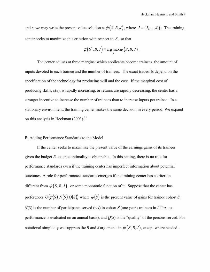
The center adjusts at three margins: which applicants become trainees, the amount of
inputs devoted to each trainee and the number of trainees. The exact tradeoffs depend on the
specification of the technology for producing skill and the cost. If the marginal cost of
producing skills, c(e), is rapidly increasing, or returns are rapidly decreasing, the center has a
stronger incentive to increase the number of trainees than to increase inputs per trainee. In a
stationary environment, the training center makes the same decision in every period. We expand
on this analysis in Heckman (2003).11
B. Adding Performance Standards to the Model
If the center seeks to maximize the present value of the earnings gains of its trainees
given the budget B, ex ante optimality is obtainable. In this setting, there is no role for
performance standards even if the training center has imperfect information about potential
outcomes. A role for performance standards emerges if the training center has a criterion
different from ( ), , ,S B Jψ or some monotonic function of it. Suppose that the center has
preferences ( ) ( ) ( )( )SQSNSU ,,ψ where ( )Sψ is the present value of gains for trainee cohort S,
N(S) is the number of participants served (≤ I) in cohort S (one year's trainees in JTPA, as
performance is evaluated on an annual basis), and Q(S) is the “quality” of the persons served. For
notational simplicity we suppress the and B J arguments in ( ), , ,S B Jψ except where needed.

Heckman, Heinrich, and Smith 10
By Q(S) we mean characteristics of the potential trainees other than their impacts. For
example, county and city governments often administer their local training centers, with the
result that staff may face pressure to serve groups targeted by the local politicians (see, for
example, Smith, 1992). At the same time, concerns about the social welfare of the least well off
among the applicant population may lead local bureaucrats to serve persons who would be
excluded by criterion (7). In the presence of these preferences for goals other than impact
maximation (that is, other than allocation based purely on efficiency concerns), or in the
presence of organizational lethargy (the on-the-job leisure enjoyed by the staff may, for example,
decrease in e), performance standards may redirect activity toward choosing the persons and
treatments that satisfy ( ).Sψ
Courty and Marschke (2003) document that a variety of performance systems currently
guide government programs. Most have the following character. The training center receives a
reward R if certain short run criteria are satisfied. An idealized version focuses on the short term
outcomes of trainees, which we operationalize as the average outcome in time period “1” for the
period “0” trainees:
( ) ( )0
1 1
1 0 1,
0
1,i
i S
S YN S ∈
= ∑Y
where the subscript on 1
1Y denotes time period “1”, while the first subscript on
1,iY denotes age
“1”, measured relative to the age of training. The “0” subscript on S indicates the current cohort
of trainees:
(8) ( )0,
1
1S τ≥Y
a threshold value, the training center gets R. Otherwise it does not.
Heckman, Heinrich, and Smith 11
Several factors motivate the use of short-term outcome measures. First, in order for a
performance standards system to be effective, it must provide quick feedback to program
managers. Feedback that arrives years after the corresponding actions by program staff is of little
use for short-term decisions, but it may have great scientific value for learning about the
parameters of the system and devising an effective performance standards system in the long run.
Second, evaluations (whether experimental or non-experimental) that seek to estimate the
counterfactual outcomes of participants, which are required to produce impact estimates, take a
long time, typically on the order of years. This is true even if the impacts they produce are short-
run impacts because of the time associated with collecting comparison group data, cleaning the
data and performing econometric analyses. Third, performance measures based on impacts are
likely to be controversial, either because of uncertainty about the econometric method utilized, in
the case of non-experimental methods, or politically, in the case of random assignment. Finally,
performance standards measures based on outcome levels generally cost much less to produce
than measures based on impacts, .
a∆ This is important, because an expensive performance
management system, even if it accomplishes something, may not accomplish enough to justify
the expense. Estimating impacts, either experimentally or non-experimentally, is technically
demanding and therefore difficult to automate. As a result, it would likely require the ongoing
intervention of expensive analysts. In contrast, as already noted, an outcome-based system can
typically rely on straightforward calculations based on administrative data. Both start-up and
operating costs are relatively low for outcomes based systems.
Reward R is used to augment the center budget for the next cohort of trainees but cannot
be used as direct bonuses to center bureaucrats – or their employees. This incentive directs

Heckman, Heinrich, and Smith 12
attention toward the short run goal of attaining ( )0,
1
1SY which may, or may not, serve to
maximize the present value of output ( ), ,S B Jψ for the current batch of JTPA trainees.
These incentives create a new intertemporal dynamic that is absent without performance
standards. Decisions by the center today affect the quality and quantity of participants today and
the resources available to the center to train tomorrow’s cohort. The center's problem changes in
the presence of the incentive constraint provided by the performance standards system. ( )0
1
1SY
is a random variable as of date “0”. Thus, the budget for the next cohort, B% , is stochastic, and is
realized only after the decision on the cohort 0
S is made. Formally,
( )( )0
0
if ;
if .
1
1
1
1
B SB
B R S
ττ
<= + ≥
%Y
Y
The reward can only be spent on the next cohort of trainees.
C. A Two-Cohort Model with Performance Standards
The analysis of a model for a training center that serves only two cohorts is particularly
simple, and provides a useful point of departure for the more complicated model we analyze
below. Assume that the budget for the first cohort is fixed at B. The choice of S0, the initial
training group, affects ( )0, ,S B Jψ as before (as well as N(S0) and Q(S0)). But it also affects the
resources available to train the next cohort in the second period.
In the second period, the agency has budget B + R if 1
1 0( )S τ≥Y , so that it meets its
performance standards. It has budget B otherwise. Thus, in this simplified two-cohort model,
the problem of the center is to pick 0
S so as to maximize

Heckman, Heinrich, and Smith 13
(9)
( ) ( ) ( )( )( ) ( ) ( ) ( )( )( ) ( ) ( ) ( )( )
1
1
0
1
0 0 0
1 1 1 1
1 0 1 1 1
1 0 0 0
1 0 1 1 1
, , , ,
1Pr | max , , , ,
1
1Pr | max , , , , ,
1
S
S
U S B J N S Q S
S U S B R J N S Q S
S U S B J N S Q S
ψ
τ ψρ
τ ψρ
+ ≥ ++
+ <+
Y
Y
where 1
1 ρ+ is a discount rate. 1
1S is the cohort selected in the second period if 1
1 0( )S τ≥Y , so
that the budget equals B R+ . 0
1S is the cohort selected in the second period if 1
1 0( )S τ<Y , so
that the budget equals B. Solving the two-cohort problem involves a two-stage maximization.
For the second period cohort, there are two possible states, corresponding to whether the first
cohort succeeds or fails relative to the performance standards. The center picks a group of
trainees for each possible budget. Given these optimal values, it picks S0 to maximize criterion
(9)—given the values of 0
1S and 1
1S selected in the first stage maximization.
Heuristically, if 0
S were a continuous variable, and (9) were differentiable in 0
S , the first
order condition would be
( ) ( ) ( )( )
( ) ( ) ( ) ( )( ) ( ) ( ) ( )( ){ }1 0
1 1
0 0 0
0
1
1 0 0 1 1 1 0 0 0
1 1 1 1 1 1
0
, , , ,0
Pr ( ) |max , , , , max , , , ,
S S
U S B J N S Q S
S
S SU S B R J N S Q S U S B N S Q S
S
ψ
τψ ψ
∂=
∂
∂ ≥+ + −
∂
YI
The first term reflects the value of 0
S in raising the current utility of the training center.
The second term captures the motivating effect of performance standards, which equals the
marginal effect of S0 on the probability of winning the award times the increase in center utility
from winning the award.12 In the two-cohort model, there is no third cohort whose budget gets
Heckman, Heinrich, and Smith 14
determined by the second cohort, so this incentive effect disappears when the center makes
decisions regarding the second cohort.
In this simple model, performance standards may distort performance. Even if the
agency would maximize present value in their absence, the performance incentives create the
possibility of distortion. If R is sufficiently large and c and ρ sufficiently small, and if 1
1 0( )Y S is
weakly or perversely correlated with present value in the absence of the performance standards,
the agency may distort its choices in serving the first cohort in order to get a reward that it can
then use to serve the second cohort. If the reward is sufficiently large, it can raise the
(discounted) present value in the second period enough to more than offset the loss in present
value in the first period. Of course, the actual solution is more complicated because the criterion
is not differentiable in S0. But this heuristic is a useful guide to the more general solution, which
is presented in Heckman (2003).
D. A Model For A Stationary Environment With Performance Standards
This simple two-cohort model abstracts from an important feature of the JTPA system,
which we now develop. In reality, training centers serve multiple cohorts of trainees over many
time periods. To take an opposite extreme to the one just considered, suppose, for analytical
simplicity, that training centers last forever, and that the environment they face is stationary.
Training centers at any point of chronological time can be in one of two states: (a) in
receipt of a bonus R, so that they have budget B+R to spend on the current cohort or (b) without
the bonus, so that they have budget B. They influence these budgetary outcomes by their choice
of S in the previous chronological time period. What they choose depends on the resources
available to the center in that period. Since the environment is stationary, and there are only two

Heckman, Heinrich, and Smith 15
states, the model is a Markovian decision problem. This means that the decision variable S does
not have to be time subscripted, just state subscripted, depending on whether or not in any given
period the budget is B or B R+ .
Define 0
V as the value function of a center without a reward in the current period and
1V as the value function for a center with a reward in the current period. Then,
1 1
0 1 1 1 0
1 1max ( ( , , ), ( ), ( )) Pr( ( ) ) Pr( ( ) )
1 1S
V U S B J N S Q S S V S Vψ τ τρ ρ
= + ≥ + <+ +
Y Y ,
where we make the budget in each state explicit by entering it as a conditioning argument in the
utility function. We define 1
V
in a parallel fashion:
1 1
1 1 1 1 0
1 1max ( ( , , ), ( ), ( )) Pr( ( ) ) Pr( ( ) )
1 1S
V U S B R J N S Q S S V S Vψ τ τρ ρ
= + + ≥ + <+ +
Y Y .
We assume that1 0
V V> , because more resources further center objectives. The optimal choice of
S depends on the rewards, the preferences, and the constraints facing centers. Here we present
an intuitive analysis of the effects of incentives. We develop this model formally in Heckman
(2003), but a number of features of it are intuitively obvious and we record them here without
proof.
(1) Let 01P be the transition probability of going from no reward to a reward and let
11P be the transition probability of having a reward in two consecutive periods. Since having
more resources makes it easier to attain all center objectives, including meeting performance
standards next period, 11 01P P> . Performance standards impart a value to incumbency.
(2) The analysis of the two-period model carries over in part in this more general setting.
With sufficiently large R, sufficiently small ρ , and sufficiently misdirected performance
incentives (incentives not aligned with present value maximization), centers that care only about
Heckman, Heinrich, and Smith 16
maximizing the present value of the earnings gains of participants may choose to divert resources
away from that goal in low budget (non-reward) periods. They will do so in order to get the
budgetary reward in the following period, which can then be spent to generate a larger total
discounted stream of earnings gains than would period-by-period earnings gain maximization.
The same incentives are not operative in high budget periods. Thus, in the case where center
preferences are the same as social preferences, if discount rates are sufficiently low, misaligned
performance standards may distort activity, but only in the low budget state.
(3) For the conditions on center preferences analyzed in point (2), and the same
misalignment of performance incentives, if the probability of attaining the reward threshold is
sufficiently low, but the reward R is sufficiently high, the introduction of performance standards
can lower the aggregate output of all centers. Unsuccessful centers divert their activities away
from productive uses and toward meeting the targets. Successful centers produce more human
capital because they have more resources. If the gains for the successful centers are sufficiently
small and the successful centers are a small fraction of all centers, aggregate output can decrease.
In general, the question of whether or not incentives distort or enhance aggregate productivity of
training centers is an empirical question on which we provide some information in this paper.
E. Cream Skimming
The most common criticism of the JTPA performance standards system, and other similar
systems, is that they encourage cream skimming. That is, by rewarding training centers based on
the mean outcomes of their participants, rather than the mean impacts of the services they
provide, the system encourages them to serve persons who will have good labor market
outcomes (as measured by the system) whether or not the program has any benefit for them, or
Heckman, Heinrich, and Smith 17
for whom there are substantial short run benefits. The performance measures create an incentive
to serve persons with a high value of 1
1,iY , regardless of whether that high value results from a
high value of 0
1,iY or a high value of ∆ 1,i . The existing literature is vague about whether cream
skimming should be defined in terms of 0
,1
1
,1 or ii
YY . The logic of performance standards in terms
of program outcomes suggests a definition in terms of 1
,1 iY .13
As noted in Heckman (1992), and Heckman, Smith, and Clements (1997), conventional
models of program evaluation assume that 1 0
, , and a i a i
Y Y differ by a constant:
1 0
, , , for all ,a i a i a i a
Y Y i∆ = − = ∆
that is, that everyone has the same impact of treatment.14 This is the so-called “common effect”
model. In this case, a high 1
,1 iY goes hand in glove with a high 0
,1 iY and picking persons with a
high 0
,1 iY helps toward satisfying (8). Assuming equal costs across all trainees, cream skimming
(or “bottom scraping” by focusing on the “hard to serve”) is innocuous, because all participants
have the same impact from the program.
Heckman, Smith, and Clements (1997) show that when the ranks of 1
,1 iY and 0
,1 iY in their
respective distributions are the same, one can relax the assumption that ∆a is the same for
everyone, but preserve many of the features of the common effect model without assuming a
common treatment effect. In this case, if ( )0
,1
1
,1
iiYY is increasing in 0
1,iY , the center has an incentive
to cream skim on 0
,1 iY . Cream skimming on the untreated outcome furthers the maximization of
the present values of earnings gains if ( ) 0
,1
0
,1
1
,1 -iii
YYY is increasing in 0
,1 iY . Cream skimming on

Heckman, Heinrich, and Smith 18
0
1,iY has the same effects as cream skimming on 1
1,iY because the two are monotonically related if
the densities of 0
1,iY and 1
1,iY are continuous.
Finally, many of the analyses in Heckman, Smith, and Clements (1997) suggest that most
of the variance in 1
1,iY is actually variance in 0
1,iY or, put differently, the variance of 1,i
∆ is small
relative to that of 0
1,iY . In this case, cream skimming based on 0
1,iY will again have essentially the
same effects on the efficiency or equity of the program's choices as cream skimming based on
1
1,iY . In general, however, the two definitions of cream skimming have different theoretical and
operational content.
III. Institutions
A. The JTPA Program
The Job Training Partnership Act program began in 1982. It envisioned a partnership
between the private, public and non-profit sectors in providing employment and training services
to the disadvantaged. Until recently, when it was replaced by the Workforce Investment Act,
JTPA was the largest federal employment and training program. The program operated through
local training centers, which usually had a local monopoly on providing JTPA services (though
not on government-subsidized employment and training services in general). JTPA was a
voluntary program (for both participants and training centers) that served persons receiving
means tested federal transfers or with a low family income in the six months preceding program
entry. Commonly provided services included classroom training in occupational skills,
subsidized on-the-job training at private firms and job search assistance. Among youth, basic
education (often leading to taking the GED exam) and work experience were also sometimes
Heckman, Heinrich, and Smith 19
provided.15 Most services were contracted out to private providers, non-profit agencies or other
government agencies (such as community colleges).
B. The JTPA Performance Standards System
The federal government, the states, and the local JTPA training centers all played distinct
roles in the JTPA system. The federal government defined core performance standard outcome
measures. These measures evolved somewhat over time, but always included employment rates,
either at termination from JTPA or 13 weeks after, and average wage rates among participants
who found employment, computed for both all participants and participants on welfare. The
simple model in Section II, which defines performance in terms of earnings levels, captures only
one of the many measures actually used, but can easily be modified for other measures, or for the
weighted average of measures actually used in the JTPA system (see Heckman, 2003). Each
program year, the federal government defined target levels, or standards, for each core outcome
measure, and provided a regression model that allowed states to adjust the targets for differences
in economic conditions and participant characteristics among centers.
The individual states could adopt the federally defined standards or modify and augment
them within broad limits. Many states added additional measures that provided incentives to
serve particular groups within the JTPA-eligible population. States also had substantial discretion
over the “award function,” the rule that determined centers' budgetary payoffs as a function of
their performance relative to the standards and, in some cases, relative to each other. As
documented in Courty and Marschke (2003), these functions varied widely among states on
many dimensions. All of the state systems shared the feature that centers were never worse off
for increasing average employment or wages among participants. For this reason, and because

Heckman, Heinrich, and Smith 20
the employment and wage rate measures typically received the greatest weight in the state award
functions, we concentrate our analysis on these measures.
The individual centers kept track of the participants' labor market outcomes, subject to
state and federal reporting rules. At the end of each program year, states calculated the
performance measures for each center and determined the reward it would receive. Depending on
the state award function and its performance, a center could receive nothing (or even a sanction
if it was far below the threshold) or, in the event of success, as much as a 20 to 30 percent
increase in its regular budget. Centers valued these award funds because they could be used more
flexibly than regular budget allocations.
C. The WIA Performance Standards System
The performance standards systems for many other programs, including employment and
training programs in Canada and Germany, resemble those in the JTPA system in their reliance
on short term outcome levels as a proxy for long term impacts. Thus our analysis has generality
well beyond the JTPA program. The performance standards system for the WIA program, the
successor to JTPA, is similar in both its federalism and in the types of performance measures it
employs. The WIA system is described in detail in U.S. Department of Labor (2000a,b) and
criticized in U.S. General Accounting Office (2002). WIA provides essentially the same services
as JTPA to a somewhat broader population. O'Shea and King (2001) describe the program in
detail. Its performance standard measures include close analogs to the JTPA measures we study
here, such as entry into unsubsidized employment and retention in unsubsidized employment six
months after entry into employment (where “retention” need not mean actually keeping the same
job).16
Heckman, Heinrich, and Smith 21
IV. The National JTPA Study Data
We use data gathered as part of the National JTPA Study, an experimental evaluation of
the JTPA program.17 The experiment was conducted at 16 of the more than 600 JTPA training
centers. At these centers, persons who applied to and were accepted into the program were
randomly assigned to either a treatment group allowed access to JTPA services or to a control
group denied access to JTPA services for the next 18 months. Background information including
demographic variables, educational attainment, work histories, indicators of previous training
and of participation in government transfer programs, and family income and composition were
collected at the time of random assignment. Survey information on employment and earnings
was collected around 18 months after random assignment and again for a sub-sample of the
experimental group around 30 months after random assignment.
V. The Efficiency Effects of Cream Skimming
In this section, we present two pieces of evidence on the efficiency effects of cream
skimming in JTPA. We then review the literature on whether or not cream skimming actually
occurs in practice.
A. Efficiency Effects of Cream Skimming on 0
aY and 1
aY .
As noted in Heckman (1992) and Heckman, Smith, and Clements (1997), experimental
data alone do not identify both components of ( )0 1,
a aY Y or their joint distribution. They only
identify the marginal distributions of 0
aY and 1
aY . We know either 0
aY (for the controls) or 1
aY (for
Heckman, Heinrich, and Smith 22
the treatments) but not both for either group. Thus, without further assumptions, it is not
possible to form 1 0
a a aY Y∆ = − for anyone or to relate it to either 0
aY or 1
aY .
Following Heckman, Smith, and Clements (1997), if the ranks of 0
aY and 1
aY for any
person are the same in their respective distributions, it is possible to associate a 0
aY with each 1
aY ,
and the association is unique if both distributions are continuous. We use this assumption to
construct a
∆ as a function of 0
aY . Given continuity of the two marginal distributions and the
perfect ranking assumption, 0( )
a aY∆ can be expressed as a function of 0
aY (or its percentile
equivalent 1
aY ). Under this assumption cream skimming on 0
aY is equivalent to cream skimming
on 1
aY .
The perfect ranking assumption is implied by the common effect assumption ,a i a
∆ = ∆
for all i but does not imply it. It generalizes the common effect assumption by allowing the
impact a
∆ to vary as a function of 0
aY . We operationalize this idea by taking percentile
differences across the treated and untreated outcome distributions.18 Let 0, j
aY denote the jth
percentile of the 0
aY distribution, with 1, j
aY the corresponding percentile in the 1
aY distribution.
Thus, we estimate ( )0, 1, 0,j j j
a a a aY Y Y∆ = − .
Figures 1A and 1B present estimates of ( )0, j
a aY∆ constructed using this method for adult
females and males, respectively. Earnings in the 18 months after random assignment constitute
the outcome. Consider first the estimates for adult women in Figure 1A, for whom the sample
size is the largest. At the low end, the impact is zero through the 20th percentile. This region
corresponds to persons with zero earnings in the 18 months after random assignment in both the
treated and untreated states. The treatment effect is flat and positive over the interval from the
Heckman, Heinrich, and Smith 23
20th to the 90th percentile, after which there is a discernible increase in the estimated impact in
the final decile. Figure 1A suggests that with equal costs per participant, the net gains from
participation are modest and roughly constant over a broad range of untreated outcomes, and that
cream skimming past the 20th percentile probably contributes little to efficiency. However, a
policy of targeting services at the bottom two deciles would likely entail considerable efficiency
costs. Figure 1B for adult men tells a similar tale. The curve is flat over the range from the 10th
to the 50th percentile, after which it dips and then begins to rise.
B. Impact Estimates and Participant Characteristics
Another way to assess the potential for efficiency losses from cream skimming is to
establish whether or not the predictors of 1
aY are correlated with measured impacts. Program
officials are likely to use characteristics ( )X to forecast the short run target outcome. The
relationship between the predictors and a
∆ is of interest in its own right. We find few precise
relationships between the predictors and the impacts and conclude that there are unlikely to be
sizeable efficiency losses from cream skimming.
Tables 1A and 1B summarize subgroup estimates of the impact of JTPA on the earnings
and employment of adult females and adult males in the JTPA experiment, respectively.19 The
first column in each table lists the values of each subgroup variable. Columns two through five
present impact estimates on 18- month and 30-month earnings and 18-month and 30-month
employment, respectively. The tables also present p-values from tests of the null of equal
impacts among subgroups for each X.
We estimated subgroup impacts conditional on labor force status (employed, unemployed
and out of the labor force) and highest grade completed, both measured at random assignment.

Heckman, Heinrich, and Smith 24
We also estimated impacts conditional on receipt of Aid to Families with Dependent Children
(AFDC)20 and on the month of last employment (if any). All of these variables predict the level
of the 18-month and 30-month outcomes for participants.
For adult females, we reject the null of equal impacts among subgroups in four of the
sixteen possible cases. The rejections (at the five percent level) occur for employment over 18
months and earnings over 30 months conditional on AFDC receipt, and over 30 months for both
earnings and employment conditional on month of last employment, with larger impacts in each
case for women receiving AFDC. However, even when we do not reject the null of equal
impacts, the point estimates suggest very different impacts, and hence the possibility of
substantial efficiency losses from cream skimming which cannot be detected in our samples. The
point estimates for the other two sets of estimates, for which the null of equality is not rejected,
suggest larger impacts for AFDC recipients. As AFDC receipt is negatively related to 1
aY , this
finding suggests that cream skimming may be (slightly) inefficient for adult women. The
interpretation of the subgroup estimates for adult females conditional on month of last
employment before random assignment is less clear, as the pattern of coefficient estimates is
non-monotonic. This finding, combined with the general lack of statistically significant subgroup
differences in impact estimates and the sometimes substantial changes in the estimated
coefficients from 18 to 30 months, suggest, at most, weak evidence of modest inefficiency
arising from cream skimming for adult females.
For adult males, statistically significant differences in impacts among subgroups defined
by X emerge only once, for impacts on 18-month earnings conditional on labor force status. In
this case, the largest impacts appear for men employed at the time of random assignment.
Employment at random assignment is positively correlated with 1
aY . As for the adult women, the
Heckman, Heinrich, and Smith 25
insignificant coefficients vary substantially among subgroups, and reveal patterns that are
difficult to interpret, such as non-monotonicity as a function of months since last employment or
years of schooling, as well as substantial changes from 18 to 30 months. Combined with the
general lack of statistically significant subgroup impacts, the pattern of estimates presents weak
evidence of at most a modest efficiency gain to cream skimming for adult males. For both men
and women, of course, the costs of service provision may vary among subgroups as well, so that
the net impacts may differ in either direction from the gross impacts reported here.
Other results in the literature that make use of the experimental data from the NJS echo
the findings in Table 1. Bloom et al. (1993, Exhibits 4.15 and 5.14) present subgroup impact
estimates on earnings in the 18 months after random assignment, while Orr et al. (1996, Exhibits
5.8 and 5.9) present similar estimates for 30-month earnings, using a somewhat different
earnings measure than we use here.21 Both consider a different set of subgroups than we do.
Only a couple of significant subgroup impacts appear at 18 months. At 30 months, the only
significant subgroup differences found by Orr et al. (1996) among adults are for adult men,
where men with a spouse present have higher impacts.22 Overall, the absence of many
statistically significant subgroup differences, combined with the pattern of point estimates,
makes the findings in Bloom et al. (1993) and Orr et al. (1996) consistent with our own findings.
There are unlikely to be substantial efficiency gains or losses from picking people on the basis of
X .23
VI. The Effects of Performance Incentives on Behavior
A. Cream-Skimming in JTPA?
Heckman, Heinrich, and Smith 26
In this section, we review the evidence on the question of whether or not cream skimming
occurs in response to the incentives presented by the JTPA performance standards system. In
order to do so, we first introduce some additional notation that will allow us to define precisely
how we can go about identifying cream skimming empirically. We define indicators for the
following stages of the JTPA participation process: E for eligibility for JTPA, W for awareness
of the JTPA program, A for application to JTPA, C for acceptance into the JTPA program and T
for formal enrollment in the JTPA program. These stages are largely self-explanatory except for
acceptance, which means that a spot in the program has been offered. Figure 2 summarizes the
stages in the JTPA participation process.
In Section II we defined cream skimming as selection of persons into the program based
on 1
1Y , and noted that empirically this is essentially the same as selection on 0
1Y . In examining
cream skimming empirically, two issues arise. The first is that we do not observe 1
1Y for non-
participants, and so we cannot directly examine the cream skimming question by comparing
values of 1
1Y for participants and non-participants or for accepted and rejected applicants. The
literature typically addresses this issue by looking at observable characteristics X that predict 1
1Y ,
either directly or in the form of a predicted value ( )XY1
1
ˆ . Addressing the cream skimming issue
in this way implicitly assumes the validity of matching on X as an estimator. If the assumptions
of matching are satisfied for X , we can use ( )1
1Y X for participants to validly approximate
( )1
1Y X for nonparticipants.
The second issue concerns what population of non-participants against which to compare
the participants. The literature adopts two approaches to this issue. The first compares
participants with the eligible population as a whole. This approach implicitly assumes that in the
Heckman, Heinrich, and Smith 27
absence of cream skimming, eligibles would participate at random, or at least not in a way that
looks like cream skimming. As a result, it potentially conflates self-selection by participants
with the exercise of administrative discretion in choosing among applicants.
As discussed in Devine and Heckman (1996), the JTPA program casts a fairly wide net in
terms of eligibility. Its eligible population includes persons with stable, low-wage employment.
As shown in Heckman and Smith (1999), such persons have very low participation probabilities.
They also have relatively high earnings within the eligible population. It is unlikely that cream
skimming is the reason why such persons fail to participate in JTPA, especially since this group
shows a low participation rate for other training programs without performance standards
(Heckman, LaLonde, and Smith, 1999). The second approach attempts to avoid this problem by
comparing participants only to applicants, on the argument that program bureaucrats have
substantially more control over who participates among applicants than over who participates
among eligibles. A potential problem with this approach is that even among applicants, there
may be self-selection out of the program into work. Further, any control that staff have over who
applies, through their marketing efforts and choice of contract providers such as non-profit
community agencies, is missed.
Anderson et al. (1992) use data on adult JTPA enrollees in Tennessee in 1987, combined
with data on persons eligible for JTPA identified in the March 1986-1988 Current Population
Surveys, to compare f(X | E = 0) with f(X | E=0, W = 0, A = 0, C = 0, T=0). Relative to all
eligibles, they find that participants are significantly more likely to be female, high school
dropouts and AFDC recipients. Within the black and AFDC recipient subgroups, JTPA
participants have much lower probabilities of being high school dropouts than eligible non-
participants. Using the same data, Anderson, et al. (1993) estimate a bivariate probit model of

Heckman, Heinrich, and Smith 28
enrollment and of placement conditional on enrollment. In this multivariate framework, less
educated eligibles (particularly high school dropouts) are under-represented in the program, but
blacks and AFDC participants are not. Their model predicts that if eligible persons participated
at random, the placement rate would fall 9.1 percentage points, from 70.7 percent to 61.6
percent, suggesting modest evidence of cream-skimming when measured relative to all eligibles.
Heckman and Smith (1995) use data from the four training centers in the JTPA
experimental study at which special data on program eligibles were collected, combined with
data from the Survey of Income and Program Participation (SIPP), to decompose the process of
JTPA participation into four stages: eligibility, awareness, application and acceptance (combined
into a single stage due to data limitations), and participation. Several findings emerge from their
study. First, the differential participation of certain groups among the eligible population has
multiple causes. For example, among the least educated (those with fewer than 10 years of
schooling), lack of awareness of JTPA plays a critical role in deterring participation. Awareness
depends only very indirectly on the efforts of JTPA staff. At the same time, adults with fewer
than 10 years of schooling are also less likely to reach the application and acceptance stage
conditional on awareness and are less likely to enroll conditional on applying and being
accepted. This evidence suggests that cream skimming may play a role in their low participation
rate. Second, Heckman and Smith (1995) provide evidence of cream skimming at the enrollment
stage, where program staff members have the most influence. Blacks, persons with less than a
high school education, persons from poorer families and those without recent employment
experience are less likely to be enrolled than others, conditional on application and acceptance.24
The Heckman and Smith (1995) study demonstrates the importance of considering both self-
Heckman, Heinrich, and Smith 29
selection and cream skimming at each stage of the participation process. They find substantial
evidence of cream skimming for some subgroups of the overall population.
In a study of an individual center, Heckman, Smith, and Taber (1996) use the JTPA
experimental data from Corpus Christi, Texas. They examine how predicted short-term earnings
levels and predicted long-term earnings impacts affect the probability that an applicant gets
accepted into the program (where acceptance is defined as reaching the point of random
assignment) by estimating Pr(T=1| E=1, W=1, A=1, E( 1
1Y | X), E (PV|X)). They estimate both
E( 1
1Y | X), defined as expected earnings in the 18 months after random assignment for
participants, and E(PV|X), defined as the expected discounted lifetime earnings gain from
participating, either gross or net of costs, using the experimental data. The transition from
application to acceptance should depend in large part on caseworker choices and thus provides
the cleanest measure of cream skimming among the existing studies. They find strong evidence
that caseworkers at Corpus Christi select negatively on E( 1
1Y | X). That is, they find that
caseworkers indulge their preferences for helping the most disadvantaged applicants rather than
responding to the incentives provided by the performance standards system. At the same time,
they find only weak evidence of positive selection on expected gains, E(PV|X). While the authors
caution against over-generalizing from a study of only one of JTPA's more than 600
heterogeneous training centers, this study demonstrates the empirical importance of negative
cream skimming by caseworkers who indulge their preferences for helping the needy.
B. Other Effects on Bureaucratic Behavior
Heinrich's (1995, 1999, 2003) analyses of the Cook County JTPA center provide
additional insights into how performance standards affect bureaucratic behavior. At this site,

Heckman, Heinrich, and Smith 30
which had a strong technocratic focus relative to other JTPA training centers, performance
incentives were passed onto service providers through performance-based contracts. Both
caseworkers and program managers were keenly aware of contractually defined performance
expectations, and placed a strong emphasis on achieving high placement rates at low cost
(Heinrich, 1995, 2003). Heinrich's (1999) analysis of the center's decisions in awarding
contracts to service providers finds that the most important factor is a service provider's past
performance relative to cost-per-placement standards in their earlier contracts. In addition,
training center administrators set much higher performance requirements in the contracts they
concluded with vendors than they themselves faced under the state performance standards
system. In essence, they insured themselves against the possibility that some providers would
fail to meet their contractual standards.
VII. How Well Do the Short Run Performance Measures Predict Long Run Impacts?
This section presents evidence from our analysis of the JTPA experimental data and from
the literature on the link between short-run outcome measures like those in the JTPA
performance standards system (versions of 1
1Y ) and the longer-term impact of the program on
participants' earnings and employment. A central question is whether the short run performance
measures based on outcomes predict long run impacts.
A. Methods
As discussed in Heckman (1992) and Heckman, Smith, and Clements (1997), without
additional assumptions, experimental data cannot be used to generate individual-level impact
estimates. Instead, we estimate subgroup mean impacts using covariates measured at the time of
Heckman, Heinrich, and Smith 31
random assignment. For adult males and females in the NJS data, we form 43 subgroups based
on the following characteristics measured at the time of random assignment: race, age, education,
marital status, employment status, receipt of AFDC, receipt of food stamps, and training center.
Individuals with complete data belong to eight subgroups, while those with incomplete data are
included in as many subgroups as their data allow. Using self-reported earnings data, we
construct total earnings over 18 and over 30 months after random assignment for each sample
member with sufficient data. We also compute the fraction of months employed (where being
employed in a month is defined as having positive earnings in that month) in each period as our
employment outcome. Using a regression framework, we construct mean-difference
experimental impact estimates for each subgroup and adjust these estimates to reflect the fact
that a substantial fraction of persons (41 percent of adult males and 37 percent of adult females)
in the treatment group dropped out and did not participate in JTPA.25,26
The JTPA performance measures we analyze are hourly wage and employment at
termination from the program and weekly earnings and employment 13 weeks after termination.
In practice, program bureaucrats obtain these outcomes by calling the participants and asking
them. We cannot do this, and instead use program termination dates from JTPA administrative
data combined with survey data on job spells to construct the performance measures. Because
program administrators do not necessarily contact participants on the exact date of termination or
follow-up, and to allow for some measurement error in the timing of the self-reported job spells,
we use a 61-day window around each date in constructing the performance measures. We
measure employment based on the presence or absence of a job spell within this window. We
calculate hourly wages and weekly earnings for employed persons only, since the corresponding
performance standards are defined only over this group. We use the highest hourly wage within

Heckman, Heinrich, and Smith 32
the window for persons holding more than one job. Earnings are averaged over the window and
are summed over jobs for persons holding multiple concurrent jobs.
We then average the constructed performance measures over each subgroup, and regress
the estimated subgroup impacts on the subgroup averages of the performance measures, using
the inverse of the Eicker-White standard errors from the impact estimation as weights in the
regression. We estimate separate regressions for each outcome (earnings and employment over
18 and 30 months) and for each performance measure.
B. Evidence from JTPA
Table 2 presents estimates of the relationship between experimental earnings and
employment impact estimates and various short-term outcomes measured at selected dates after
random assignment. The four columns of estimates in Table 2 correspond to cumulated earnings
and employment gains over the eighteen and thirty month intervals following random
assignment. Each cell in the table presents the regression coefficient associated with the column's
dependent variable and the row's independent variable, the estimated (robust) standard error of
the coefficient, the p-value from a test of the null hypothesis that the population coefficient is
zero and the R2 for the regression. The constant from the regression is omitted to reduce clutter.
For example, the first row of the first column reveals that a regression of earnings over the 18
months after random assignment on the hourly wage at termination from the JTPA program
yields an estimated coefficient of $465.41 on the hourly wage, with a standard error of $394.76,
a p-value of 0.2452 and an overall R2 of 0.0328.
Four striking findings emerge from Table 2. First, and most important, we find many
negative relationships between short run performance indicators and the experimental impact

Heckman, Heinrich, and Smith 33
estimates. That is, in many cases, the short-term outcome measures utilized in the JTPA
performance standards system are perversely related to the longer-term participant earnings and
employment gains that constitute the program's goals. The only evidence supporting the efficacy
of short-term outcome measures is the link between employment at follow-up and earnings,
which is positive at 18 months and positive and marginally statistically significant at 30 months
for adult men (but statistically insignificant in both cases for adult women, with a negative
coefficient estimate at 30 months). Second, the R2 values are quite low. The short-term
performance standards measures are only weakly related to the long-term earnings and
employment gains produced by the program. Third, moving from wage measures at termination
to “longer-term” measures constructed from follow-up interviews at three months after
termination usually weakens the relationship between the performance standard measure and the
longer-run earnings or employment impacts. The R2 values nearly always decline and the
estimated coefficients sometimes become less positive or more negative. Fourth, the
performance measures often do worse at predicting earnings impacts estimated over 30 months
than at predicting earnings gains estimated over only the first 18 months after random
assignment. This suggests that our findings are not due to the fact that the in-program period,
when some participants reduce their labor supply to focus on training, may dominate the 18-
month outcomes of some participants.
C. Evidence from the Literature
The findings presented in the preceding subsection do not represent an anomaly in the
literature, but rather characterize the findings of almost all of the small number of existing papers
that perform similar analyses. Table 3 summarizes five other studies we found in the literature

Heckman, Heinrich, and Smith 34
that examine the relationship between performance standards measures based on short run
outcome levels and long run program impacts.27 For each study, the first column of the table
gives the citation, while the second indicates the particular employment and training program
considered. The third column indicates the data used. The fourth and fifth columns indicate the
impact measure used (for example, earnings from 18 to 36 months after leaving the program) and
what impact estimator (for example random assignment) was used to generate the impact
estimates, respectively. The sixth column details the particular performance measures
considered (for example, employment at termination from the program). The final column
summarizes the findings.
The studies range from strongly negative in their findings, as in Gay and Borus (1980),
Cragg (1997), and Burghardt and Schochet (2001), to more mixed findings such as those
reported in Friedlander (1988) and Zornitsky, et al. (1988). The most positive of the studies,
Zornitsky, et al. (1988), examines a single treatment program treating relatively homogeneous
clients, a context very different from, and perhaps not generalizable to, multi-treatment programs
serving heterogeneous populations such as JTPA and WIA. This narrowly focused program
focused on the skills for a particular occupation, and so did not stimulate post-program human
capital investment, which, as we have already noted, would weaken the relationship between the
short run performance measures and long run impacts. Taken together, these studies generally
support our finding from the JTPA data that performance standards based on short-term outcome
levels likely do little to encourage the provision of services to those who benefit most from them
in employment and training programs.
VIII. Conclusions
Heckman, Heinrich, and Smith 35
Performance standards systems that attempt to motivate bureaucratic behavior by
rewarding government agencies on the basis of short-run outcome measures are widely perceived
to be a solution to the problem of inefficiency in government, despite the absence of any strong
evidence that such standards lead bureaucrats to increase their attainment of long-run program
goals. We present a model of training center behavior in the presence of performance standards,
and show why these standards focus on short-term outcomes. Within the context of this model,
we precisely define cream skimming and show how such systems provide an incentive for it.
Our empirical analysis reaches two important conclusions. First, whatever cream
skimming occurs in JTPA produces only modest efficiency gains or losses. Opposition to cream
skimming must come on equity grounds. Put differently, our results show that the efficiency cost
of not cream skimming, and instead focusing on the hard to serve among the eligible population,
is a modest one.
Our second important conclusion is that the JTPA performance standards do not promote
efficiency because the short-term outcomes they rely on have essentially a zero correlation with
long-term impacts on employment and earnings. This surprising result comports with the
findings in several other studies that have estimated this relationship.
Nothing in this paper says that a successful performance standards system cannot be
devised. The available evidence suggests that bureaucrats respond to performance standards,
although sometimes perversely so. The available evidence also suggests that the efficiency gains
or losses from cream skimming are likely to be small. However, the performance systems that
have been tried in the past have generally used short run target measures that are only weakly
related to long run efficiency measures. If performance standards are to be put in place that

Heckman, Heinrich, and Smith 36
motivate efficiency, long term studies should be conducted to determine which short run
measures are strongly related to long term efficiency criteria.

Heckman, Heinrich, and Smith 37
References
Anderson, Kathryn, Richard Burkhauser, Jennie Raymond, and Clifford Russell. 1992. “Mixed
Signals in the Job Training Partnership Act.” Growth and Change 22(3): 32-48.
Anderson, Kathryn, Richard Burkhauser, and Jennie Raymond. 1993. “The Effect of Creaming on
Placement Rates Under the Job Training Partnership Act.” Industrial and Labor Relations Review
46(4): 613-624.
Barnow, Burt. 1992. “The Effects of Performance Standards on State and Local Programs.” In
Evaluating Welfare and Training Programs, ed. Charles Manski and Irwin Garfinkel, 277-309.
Cambridge, MA: Harvard University Press.
Becker, Gary. 1964. Human Capital. New York, NY: Columbia University Press.
Bell, Stephen, and Larry Orr. 2002. “Screening (and Creaming?) Applicants to Job Training
Programs: The AFDC Homemaker-Home Health Aide Demonstration.” Labour Economics
Forthcoming.
Bloom, Howard, Larry Orr, George Cave, Steve Bell, and Fred Doolittle. 1993. The National JTPA
Study: Title IIA Impacts on Earnings and Employment at 18 Months. Bethesda, MD: Abt
Associates.
Heckman, Heinrich, and Smith 38
Bloom, Howard, Larry Orr, Stephen Bell, George Cave, Fred Doolittle, Winston Lin, and Johannes
Bos. 1997. “The Benefits and Costs of JTPA Title II-A Programs: Key Findings from the National
Job Training Partnership Act Study.” Journal of Human Resources 32(3): 549-576.
Burghardt, John, and Peter Schochet. 2001. National Job Corps Study: Impacts by Center
Characteristics. Princeton, NJ: Mathematica Policy Research.
Carneiro, Pedro, Karsten Hansen, and James Heckman. 2001. “Educational Attainment and Labor
Market Outcomes: Estimating the Distributions of Returns to Interventions.” Unpublished
manuscript, University of Chicago.
Courty, Pascal, and Gerald Marschke. 1996. “Moral Hazard Under Incentive Systems: The Case of
a Federal Bureaucracy.” In Advances in the Study of Entrepreneurship, Innovation and Economic
Growth, Volume 7, Reinventing Government and the Problem of Bureaucracy, ed. Gary Libecap,
157-190. Greenwich, CT: JAI Press.
__________. 1997. “Measuring Government Performance: Lessons from a Federal Job Training
Program.” American Economic Review 87(2): 383-388.
__________. 2003. “The JTPA Incentive System.'' In Performance Standards in a Government
Bureaucracy: Analytic Essays on the JTPA Performance Standards System, ed. James Heckman,
forthcoming. Kalamazoo, MI: W.E. Upjohn Institute for Employment Research.
Heckman, Heinrich, and Smith 39
Cragg, Michael. 1997. “Performance Incentives in the Public Sector: Evidence from the Job
Training Partnership Act.” Journalof Law, Economics and Organization 13(1): 147-168.
Csörgö, Miklós. 1983. Quantile Processes with Statistical Applications. Philadelphia, PA:
Society for Industrial and Applied Mathematics.
Devine, Theresa, and James Heckman. 1996. “The Structure and Consequences of Eligibility Rules
for a Social Program.” In Research in Labor Economics, Volume 15, ed. Solomon Polachek, 111-
170. Greenwich, CT: JAI Press.
Dixit, Avinash. 2002. “Incentives and Organizations in the Public Sector: An Interpretative
Review.” Journal of Human Resources, current issue.
Doolittle, Fred, and Linda Traeger. 1990. Implementing the National JTPA Study. New York, NY:
Manpower Demonstration Research Corporation.
Friedlander, Daniel. 1988. Subgroup Impacts and Performance Indicators for Selected Welfare
Employment Programs. New York: Manpower Demonstration Research Corporation.
Gay, Robert, and Michael Borus. 1980. “Validating Performance Indicators for Employment and
Training Programs.” Journal of Human Resources 15(1): 29-48.
Heckman, Heinrich, and Smith 40
Hansen, Karsten, James Heckman, and Edward Vytlacil. 2000. “Dynamic Treatment Effects.”
Paper presented at the Midwest Econometrics Group, Chicago.
Hanushek, Eric. 2002. “Publically Provided Education.” In Handbook of Public Finance, ed. Alan
Auerbach and Martin Feldstein, forthcoming. Amsterdam: North-Holland.
Heckman, James. 1992. “Randomization and Social Program Evaluation.” In Evaluating Welfare
and Training Programs, ed. Charles Manski and Irwin Garfinkel, 201-230. Cambridge, MA:
Harvard University Press.
__________. 2001. “Micro Data, Heterogeneity, and the Evaluation of Public Policy: Nobel
Lecture.” Journal of Political Economy 109(4): 673-748.
_________, ed. 2003. Performance Standards in a Government Bureaucracy: Analytic Essays on
the JTPA Performance Standards System, forthcoming. Kalamazoo, MI: W.E. Upjohn Institute for
Employment Research.
Heckman, James, Neil Hohmann, Jeffrey Smith, and Michael Khoo. 2000. “Substitution and
Dropout Bias in Social Experiments: A Study of an Influential Social Experiment.” Quarterly
Journal of Economics 105(2): 651-694.
Heckman, James, Robert LaLonde, and Jeffrey Smith. 1999. “The Economics and Econometrics of
Heckman, Heinrich, and Smith 41
Active Labor Market Programs.” In Handbook of Labor Economics, Volume 3A, ed. Orley
Ashenfelter and David Card, 1865-2097. Amsterdam: North-Holland.
Heckman, James, Lance Lochner, and Christopher Taber. 1998. “Explaining Rising Wage
Inequality: Explorations with a Dynamic General Equilibrium Model of Labor Earnings with
Heterogeneous Agents.” Journal of Economic Dynamics 1(1): 1-58.
Heckman, James and Jeffrey Smith. 1995. “The Determinants of Participation in a Social Program:
Evidence from JTPA.” Unpublished manuscript, University of Chicago.
__________. 1999. “The Pre-Programme Dip and the Determinants of Participation in a Social
Program: Implications for Simple Programme Evaluation Strategies.” Economic Journal 109(457):
313-348.
Heckman, James, Jeffrey Smith, and Nancy Clements. 1997. “Making The Most Out of Programme
Evaluations and Social Experiments: Accounting for Heterogeneity in Programme Impacts.”
Review of Economic Studies 64(4): 487-535.
Heckman, James, Jeffrey Smith, and Christopher Taber. 1996. “What Do Bureaucrats Do? The
Effects of Performance Standards and Bureaucratic Preferences on Acceptance into the JTPA
Program.” In Advances in the Study of Entrepreneurship, Innovation and Economic Growth,
Volume 7, Reinventing Government and the Problem of Bureaucracy, ed. Gary Libecap, 191-218.
Greenwich, CT: JAI Press.
Heckman, Heinrich, and Smith 42
__________. 1998. “Accounting for Dropouts in Evaluations of Social Programs.” Review of
Economics and Statistics 80(1): 1-14.
Heinrich, Carolyn. 1995. “Public Policy and Methodological Issues in the Design and Evaluation of
Employment and Training Programs at the Service Delivery Area Level.” Ph.D. dissertation, Harris
School of Public Policy Studies, University of Chicago.
__________. 1999. “Do Bureaucrats Make Effective Use of Performance Management
Information?” Journal of Public Administration Research and Theory 9(3): 363-393.
__________. 2003. “The Role of Performance Standards in JTPA Program Administration and
Service Delivery at the Local Level.” In Performance Standards in a Government Bureaucracy:
Analytic Essays on the JTPA Performance Standards System, ed. James Heckman, forthcoming.
Kalamazoo, MI: W.E. Upjohn Institute for Employment Research.
Hotz, V. Joseph. 1992. “Designing an Evaluation of the Job Training Partnership Act.” In
Evaluating Welfare and Training Programs, ed. Charles Manski and Irwin Garfinkel, 76-114.
Cambridge, MA: Harvard University Press.
Hotz, V. Joseph, Guido Imbens, and Jacob Klerman. 2000. “The Long Term Gains from GAIN: A
Re-Analysis of the Impacts of the California GAIN Program.” NBER Working Paper #2007.

Heckman, Heinrich, and Smith 43
Kemple, James, Fred Doolittle, and John Wallace. 1993. The National JTPA Study: Site
Characteristics and Participation Patterns. New York: Manpower Demonstration Research
Corporation.
Mincer, Jacob. 1972. Schooling, Experience and Earnings. Chicago, IL: University of Chicago
Press.
National Commission for Employment Policy. 1995. Understanding Federal Training and
Employment Programs. Washington, DC: National Commission for Employment Policy.
Orr, Larry, Howard Bloom, Stephen Bell, Fred Doolittle, Winston Lin, and George Cave. 1996.
Does Training for the Disadvantaged Work? Evidence from the National JTPA Study. Washington,
DC: Urban Institute Press.
O'Shea, Daniel, and Christopher King. 2001. “The Workforce Investment Act of 1998.”
Rockefeller Institute Report No. 12. New York: Rockefeller Institute.
Smith, Jeffrey. 1992. “The JTPA Selection Process: A Descriptive Analysis.” Unpublished
manuscript, University of Chicago.
U.S. Congress. Government Performance and Results Act, 1993. Washington D.C.: U.S. Congress.
Heckman, Heinrich, and Smith 44
U.S. General Accounting Office. 2002. “Workforce Investment Act: Improvements Needed in
Performance Measures to Provide a More Accurate Picture of WIAs Effectiveness.” GAO-02-275.
Washington D.C.: U.S. General Accounting Office.
U.S. Department of Labor. 2000a. “Core and Customer Satisfaction Performance Measures for the
Workforce Investment System.” Training and Employment Guidance Letter No. 7-99. Washington
D.C.: Employment and Training Administration.
__________. 2000b. “Negotiating Performance Goals; and Incentives and Sanctions Process under
Title I of the Workforce Investment Act.” Training and Employment Guidance Letter No. 8-99.
Washington D.C.: Employment and Training Administration.
Wilson, James. 1989. Bureaucracy: What Government Agencies Do and Why They Do It. New
York, NY: Basic Books.
Zornitsky, Jeffrey, Mary Rubin, Stephen Bell, and William Martin. 1988. “Establishing a
Performance Management System for Targeted Welfare Programs.” National Commission for
Employment Policy Research Report 88-14.

Heckman, Heinrich, and Smith 45
1 See Hanushek (2002) for a discussion of accountability systems in education based on
performance standards at the teacher and school level. See Barnow (1992) for a discussion of
performance standards in publicly provided training programs
2 Wilson (1989) and Dixit (2002) discuss conflicts in the objectives of programs as outcomes of a
political process.
3 See Becker (1964), Mincer (1972), Heckman, Hohmann, Smith, and Khoo (2000) and Hotz,
Imbens, and Klerman (2000).
4 We abstract from decisions regarding the timing of training. See Hansen, Heckman and Vytlacil
(2000).
5 It can also be negative in the long run, as indeed it was for male youth in JTPA. See, for
example, Bloom et al. (1993).
6 Heckman, Lochner, and Taber (1998) present evidence on the importance of general equilibrium
effects in evaluating large scale educational programs. Such effects are much less likely to be
important for smaller scale job training programs.
7 Note that r may be a social discount factor.
8 We assume interior solutions. Sufficient conditions for an interior solution are concavity of (2) in
e for all 0
,a iY , convexity of ci(ei) for each i, and Inada conditions on both cost and technology. For
some S, the constraint (4) may be slack (that is, λ = 1 can be obtained).
9 There may be more than one S that qualifies. If so, we assume the training center picks the
particular set chosen at random.

Heckman, Heinrich, and Smith 46
10 Carneiro, Hansen, and Heckman (2001) demonstrate that most of the variation in future earnings
gains is unforecastable, even for college graduates. Bell and Orr (2002) show that caseworkers do a
poor job of predicting a
∆ in a program that provided job training to welfare recipients.
11 There is an additional stage to the allocation process that we do not consider, namely, the
allocation of the overall budget among centers. The budget should be allocated to equate returns at
the margin for all centers.
12 In this heuristic problem, we assume that the second order conditions are satisfied.
13 In thinking about cream skimming from a policy perspective, two other facts should be kept in
mind. First, even if cream skimming occurs, the cream of the JTPA eligible (or applicant)
population was still disadvantaged. They must have been so in order to satisfy JTPA’s eligibility
rules. Thus, cream skimming did not mean that JTPA resources got spent on, for example, middle
class people. Second, JTPA was far from the only employment and training program available at
the time (just as WIA is far from the only program available now). As documented in National
Commission for Employment Policy (1995), dozens of other programs coexisted with JTPA.
These other programs may well have provided services better suited to the hard to serve among
JTPA’s eligible population than did JTPA. Determining whether cream skimming, should it occur,
is good or bad, requires more thought than the literature typically devotes to it.
14 In models with regressors, this assumption is 1 0
, , ,( ) ( ) for all ,a i a i a i a
X Y Y X i∆ = − = ∆ yielding
equal impacts for all persons with the same X.
15 See Devine and Heckman (1996) for a detailed study of JTPA program eligibility and Orr et al.
(1996) or Kemple, Doolittle, and Wallace (1993) for details on the types of services provided and
their relative frequency.

Heckman, Heinrich, and Smith 47
16 In addition, it includes measures related to skill or credential attainment (as did JTPA), a
measure of before-after earnings changes, and measures based on “customer” satisfaction surveys.
17 Doolittle and Traeger (1990), Hotz (1992) and Orr et al. (1996) describe the design of the
experiment. Bloom et al. (1997) summarize the experimental impact estimates.
18 See Heckman, Smith, and Clements (1997) for more details on this estimator, including the
construction of the standard errors.
19 We omit analyses for male and female youth throughout the paper due to the small sample sizes
available for these groups.
20 AFDC is now called Temporary Aid to Needy Families or TANF.
21 Their earnings measure combines self-report data with data from UI earnings records. For more
details, see the discussion in Orr et al. (1996).
22 Orr et al. (1996) also present subgroup impact estimates for male and female youth (see Exhibits
5.19 and 5.20). As expected given the small sample sizes, they find no statistically significant
differences in estimated impacts among the subgroups.
23 The analyses in both this section and the preceding section have the potential limitation that they
condition on persons who reach random assignment. In choosing whom to serve, program staff
members care about relationships conditional on application to the program, not on reaching
random assignment.
24 However, even at this stage, self-selection cannot be entirely ruled out.
25 See the discussions in Heckman, Smith, and Taber (1998) and Heckman, LaLonde, and Smith
(1999, Section 5.2) on the origin of this estimator.

Heckman, Heinrich, and Smith 48
26 An alternative strategy would generate predicted individual impacts by including interaction
terms between baseline covariates and the treatment group dummy in an impact regression.
27 We thank Tim Bartik of the Upjohn Institute for providing us with copies of two of the
unpublished papers.
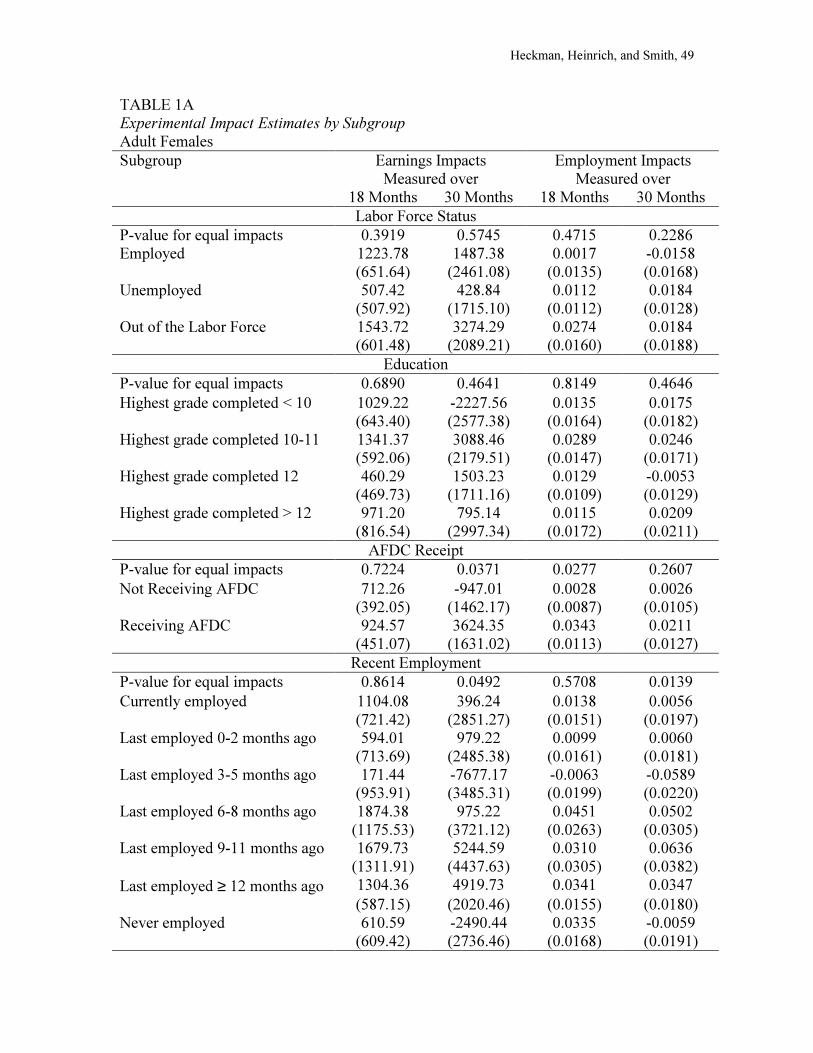
Heckman, Heinrich, and Smith, 49
TABLE 1A
Experimental Impact Estimates by Subgroup
Adult Females
Subgroup Earnings Impacts
Measured over
Employment Impacts
Measured over
18 Months 30 Months 18 Months 30 Months
Labor Force Status
P-value for equal impacts 0.3919 0.5745 0.4715 0.2286
Employed 1223.78 1487.38 0.0017 -0.0158
(651.64) (2461.08) (0.0135) (0.0168)
Unemployed 507.42 428.84 0.0112 0.0184
(507.92) (1715.10) (0.0112) (0.0128)
Out of the Labor Force 1543.72 3274.29 0.0274 0.0184
(601.48) (2089.21) (0.0160) (0.0188)
Education
P-value for equal impacts 0.6890 0.4641 0.8149 0.4646
Highest grade completed < 10 1029.22 -2227.56 0.0135 0.0175
(643.40) (2577.38) (0.0164) (0.0182)
Highest grade completed 10-11 1341.37 3088.46 0.0289 0.0246
(592.06) (2179.51) (0.0147) (0.0171)
Highest grade completed 12 460.29 1503.23 0.0129 -0.0053
(469.73) (1711.16) (0.0109) (0.0129)
Highest grade completed > 12 971.20 795.14 0.0115 0.0209
(816.54) (2997.34) (0.0172) (0.0211)
AFDC Receipt
P-value for equal impacts 0.7224 0.0371 0.0277 0.2607
Not Receiving AFDC 712.26 -947.01 0.0028 0.0026
(392.05) (1462.17) (0.0087) (0.0105)
Receiving AFDC 924.57 3624.35 0.0343 0.0211
(451.07) (1631.02) (0.0113) (0.0127)
Recent Employment
P-value for equal impacts 0.8614 0.0492 0.5708 0.0139
Currently employed 1104.08 396.24 0.0138 0.0056
(721.42) (2851.27) (0.0151) (0.0197)
Last employed 0-2 months ago 594.01 979.22 0.0099 0.0060
(713.69) (2485.38) (0.0161) (0.0181)
Last employed 3-5 months ago 171.44 -7677.17 -0.0063 -0.0589
(953.91) (3485.31) (0.0199) (0.0220)
Last employed 6-8 months ago 1874.38 975.22 0.0451 0.0502
(1175.53) (3721.12) (0.0263) (0.0305)
Last employed 9-11 months ago 1679.73 5244.59 0.0310 0.0636
(1311.91) (4437.63) (0.0305) (0.0382)
Last employed ≥ 12 months ago 1304.36 4919.73 0.0341 0.0347
(587.15) (2020.46) (0.0155) (0.0180)
Never employed 610.59 -2490.44 0.0335 -0.0059
(609.42) (2736.46) (0.0168) (0.0191)

Heckman, Heinrich, and Smith, 50
Source: Authors’ calculations using National JTPA Study data.
Notes: Monthly earnings are based on self-reports with top 1% trimming. Estimates are
adjusted for program dropouts in the treatment group. Earnings impacts are calculated
using all sample members with valid observations for self-reported monthly earnings
during each period. The sample includes 4886 valid observations for the 18-month
period after random assignment and 1147 valid observations for the 30-month period
after random assignment. Robust standard errors appear in parentheses.
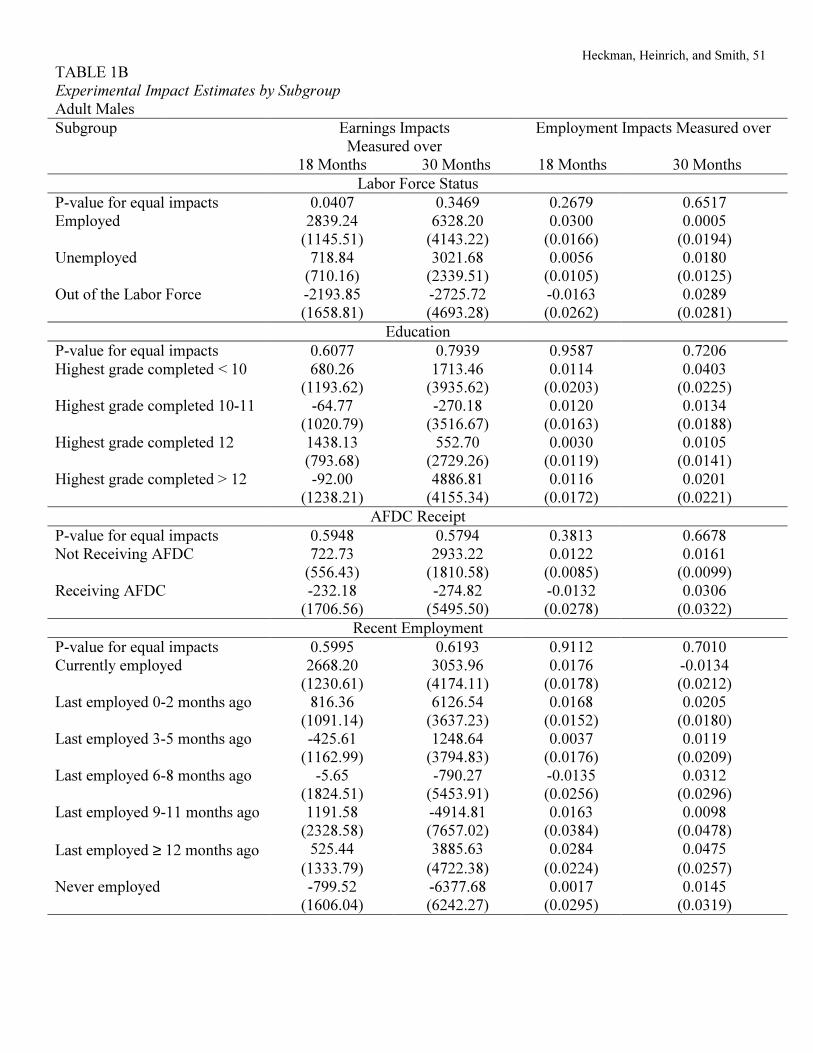
Heckman, Heinrich, and Smith, 51
TABLE 1B
Experimental Impact Estimates by Subgroup
Adult Males
Subgroup Earnings Impacts
Measured over
Employment Impacts Measured over
18 Months 30 Months 18 Months 30 Months
Labor Force Status
P-value for equal impacts 0.0407 0.3469 0.2679 0.6517
Employed 2839.24 6328.20 0.0300 0.0005
(1145.51) (4143.22) (0.0166) (0.0194)
Unemployed 718.84 3021.68 0.0056 0.0180
(710.16) (2339.51) (0.0105) (0.0125)
Out of the Labor Force -2193.85 -2725.72 -0.0163 0.0289
(1658.81) (4693.28) (0.0262) (0.0281)
Education
P-value for equal impacts 0.6077 0.7939 0.9587 0.7206
Highest grade completed < 10 680.26 1713.46 0.0114 0.0403
(1193.62) (3935.62) (0.0203) (0.0225)
Highest grade completed 10-11 -64.77 -270.18 0.0120 0.0134
(1020.79) (3516.67) (0.0163) (0.0188)
Highest grade completed 12 1438.13 552.70 0.0030 0.0105
(793.68) (2729.26) (0.0119) (0.0141)
Highest grade completed > 12 -92.00 4886.81 0.0116 0.0201
(1238.21) (4155.34) (0.0172) (0.0221)
AFDC Receipt
P-value for equal impacts 0.5948 0.5794 0.3813 0.6678
Not Receiving AFDC 722.73 2933.22 0.0122 0.0161
(556.43) (1810.58) (0.0085) (0.0099)
Receiving AFDC -232.18 -274.82 -0.0132 0.0306
(1706.56) (5495.50) (0.0278) (0.0322)
Recent Employment
P-value for equal impacts 0.5995 0.6193 0.9112 0.7010
Currently employed 2668.20 3053.96 0.0176 -0.0134
(1230.61) (4174.11) (0.0178) (0.0212)
Last employed 0-2 months ago 816.36 6126.54 0.0168 0.0205
(1091.14) (3637.23) (0.0152) (0.0180)
Last employed 3-5 months ago -425.61 1248.64 0.0037 0.0119
(1162.99) (3794.83) (0.0176) (0.0209)
Last employed 6-8 months ago -5.65 -790.27 -0.0135 0.0312
(1824.51) (5453.91) (0.0256) (0.0296)
Last employed 9-11 months ago 1191.58 -4914.81 0.0163 0.0098
(2328.58) (7657.02) (0.0384) (0.0478)
Last employed ≥ 12 months ago 525.44 3885.63 0.0284 0.0475
(1333.79) (4722.38) (0.0224) (0.0257)
Never employed -799.52 -6377.68 0.0017 0.0145
(1606.04) (6242.27) (0.0295) (0.0319)

Heckman, Heinrich, and Smith, 52
Source: Authors’ calculations using National JTPA Study data.
Notes: Monthly earnings are based on self-reports with top 1% trimming. Estimates are adjusted for program
dropouts in the treatment group. Earnings impacts are calculated using all sample members with valid
observations for self-reported monthly earnings during each period. The sample includes 4886 valid
observations for the 18-month period after random assignment and 1147 valid observations for the 30-month
period after random assignment. Robust standard errors appear in parentheses.
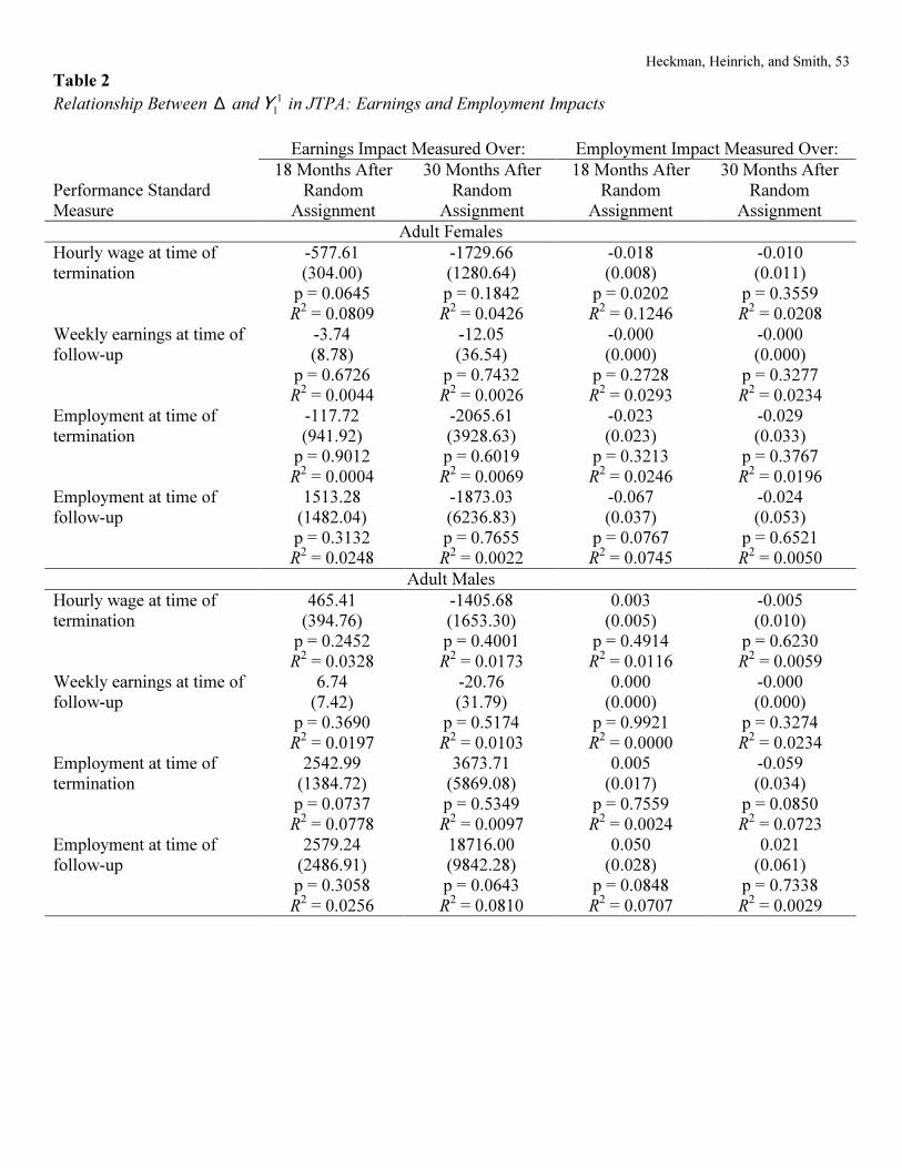
Heckman, Heinrich, and Smith, 53
Table 2
Relationship Between ∆ and 1
1Y in JTPA: Earnings and Employment Impacts
Earnings Impact Measured Over: Employment Impact Measured Over:
Performance Standard
Measure
18 Months After
Random
Assignment
30 Months After
Random
Assignment
18 Months After
Random
Assignment
30 Months After
Random
Assignment
Adult Females
Hourly wage at time of
termination
-577.61
(304.00)
p = 0.0645
R2 = 0.0809
-1729.66
(1280.64)
p = 0.1842
R2 = 0.0426
-0.018
(0.008)
p = 0.0202
R2 = 0.1246
-0.010
(0.011)
p = 0.3559
R2 = 0.0208
Weekly earnings at time of
follow-up
-3.74
(8.78)
p = 0.6726
R2 = 0.0044
-12.05
(36.54)
p = 0.7432
R2 = 0.0026
-0.000
(0.000)
p = 0.2728
R2 = 0.0293
-0.000
(0.000)
p = 0.3277
R2 = 0.0234
Employment at time of
termination
-117.72
(941.92)
p = 0.9012
R2 = 0.0004
-2065.61
(3928.63)
p = 0.6019
R2 = 0.0069
-0.023
(0.023)
p = 0.3213
R2 = 0.0246
-0.029
(0.033)
p = 0.3767
R2 = 0.0196
Employment at time of
follow-up
1513.28
(1482.04)
p = 0.3132
R2 = 0.0248
-1873.03
(6236.83)
p = 0.7655
R2 = 0.0022
-0.067
(0.037)
p = 0.0767
R2 = 0.0745
-0.024
(0.053)
p = 0.6521
R2 = 0.0050
Adult Males
Hourly wage at time of
termination
465.41
(394.76)
p = 0.2452
R2 = 0.0328
-1405.68
(1653.30)
p = 0.4001
R2 = 0.0173
0.003
(0.005)
p = 0.4914
R2 = 0.0116
-0.005
(0.010)
p = 0.6230
R2 = 0.0059
Weekly earnings at time of
follow-up
6.74
(7.42)
p = 0.3690
R2 = 0.0197
-20.76
(31.79)
p = 0.5174
R2 = 0.0103
0.000
(0.000)
p = 0.9921
R2 = 0.0000
-0.000
(0.000)
p = 0.3274
R2 = 0.0234
Employment at time of
termination
2542.99
(1384.72)
p = 0.0737
R2 = 0.0778
3673.71
(5869.08)
p = 0.5349
R2 = 0.0097
0.005
(0.017)
p = 0.7559
R2 = 0.0024
-0.059
(0.034)
p = 0.0850
R2 = 0.0723
Employment at time of
follow-up
2579.24
(2486.91)
p = 0.3058
R2 = 0.0256
18716.00
(9842.28)
p = 0.0643
R2 = 0.0810
0.050
(0.028)
p = 0.0848
R2 = 0.0707
0.021
(0.061)
p = 0.7338
R2 = 0.0029

Heckman, Heinrich, and Smith, 54
Source: Authors’ calculations using National JTPA Study data.
Notes: The actual JTPA performance measures are defined as follows: “Hourly Wage at Placement” is the
average wage at program termination for employed adults. “Weekly Earnings at Follow-up” are the average
weekly wage of adults employed 13 weeks after program termination. “Employment Rate at Placement” is the
fraction of adults employed at program termination. “Employment Rate at Follow-up” is the fraction of adults
who were employed 13 weeks after program termination. In our analysis, employment rates were calculated
based on the presence or absence of a job spell within 30 days of each reference date (termination or follow-up).
Hourly wages were calculated based on the highest reported hourly wage for all job spells reported within 30
days of each reference date. Weekly earnings were calculated by averaging the product of hourly wages and
hours worked per week across all reported job spells within 30 days of each reference date weighted by the
fraction of the 30-day window spanned by each job spell.
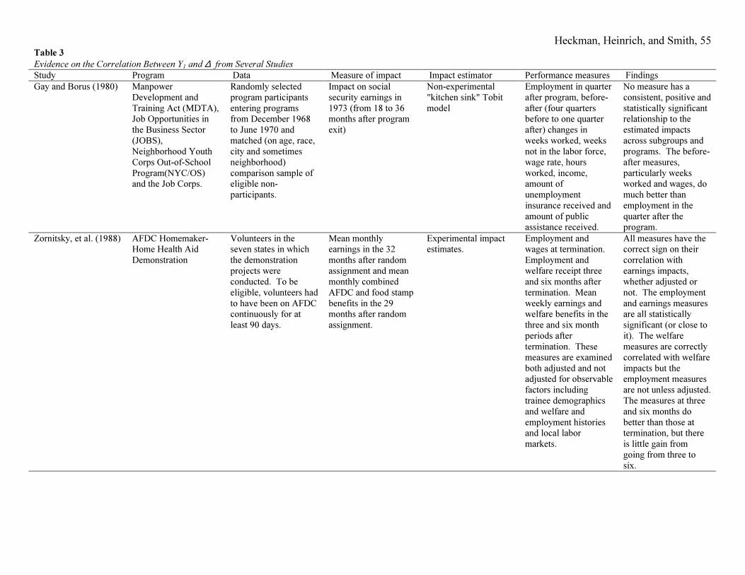
Heckman, Heinrich, and Smith, 55 Table 3
Evidence on the Correlation Between Y1 and ∆ from Several Studies
Study Program Data Measure of impact Impact estimator Performance measures Findings
Gay and Borus (1980) Manpower
Development and
Training Act (MDTA), Job Opportunities in
the Business Sector
(JOBS),
Neighborhood Youth
Corps Out-of-School
Program(NYC/OS) and the Job Corps.
Randomly selected
program participants
entering programs from December 1968
to June 1970 and
matched (on age, race,
city and sometimes
neighborhood)
comparison sample of eligible non-
participants.
Impact on social
security earnings in
1973 (from 18 to 36 months after program
exit)
Non-experimental
"kitchen sink" Tobit
model
Employment in quarter
after program, before-
after (four quarters before to one quarter
after) changes in
weeks worked, weeks
not in the labor force,
wage rate, hours
worked, income, amount of
unemployment
insurance received and
amount of public
assistance received.
No measure has a
consistent, positive and
statistically significant relationship to the
estimated impacts
across subgroups and
programs. The before-
after measures,
particularly weeks worked and wages, do
much better than
employment in the
quarter after the
program.
Zornitsky, et al. (1988) AFDC Homemaker-Home Health Aid
Demonstration
Volunteers in the seven states in which
the demonstration
projects were
conducted. To be
eligible, volunteers had
to have been on AFDC continuously for at
least 90 days.
Mean monthly earnings in the 32
months after random
assignment and mean
monthly combined
AFDC and food stamp
benefits in the 29 months after random
assignment.
Experimental impact estimates.
Employment and wages at termination.
Employment and
welfare receipt three
and six months after
termination. Mean
weekly earnings and welfare benefits in the
three and six month
periods after
termination. These
measures are examined
both adjusted and not adjusted for observable
factors including
trainee demographics
and welfare and
employment histories and local labor
markets.
All measures have the correct sign on their
correlation with
earnings impacts,
whether adjusted or
not. The employment
and earnings measures are all statistically
significant (or close to
it). The welfare
measures are correctly
correlated with welfare
impacts but the employment measures
are not unless adjusted.
The measures at three
and six months do
better than those at termination, but there
is little gain from
going from three to
six.

Heckman, Heinrich, and Smith, 56
Table 3 (Continued)
Evidence on the Correlation Between Y1 and ∆ from Several Studies
Study Program Data Measure of impact Impact estimator Performance measures Findings
Friedlander (1988) Mandatory welfare-to-
work programs in San
Diego, Baltimore, Virginia, Arkansas,
and Cook County.
Applicants and
recipients of AFDC
(varies across programs). Data
collected as part of
MDRC's experimental
evaluations of these
programs.
Post random
assignment earnings
(from UI earnings records) and welfare
receipt (from
administrative data).
Experimental impact
estimates.
Employment (non-zero
quarterly earnings) in
quarters 2 and 3 (short-term) or quarters 4 to 6
(long term) after
random assignment.
Welfare receipt in
quarter 3 (short-term) or quarter 6 (long-
term) after random
assignment.
Employment measure
is positively correlated
with earnings gains but not welfare savings for
most programs.
Welfare indicator is
always positively
correlated with earnings impacts, but
rarely significantly so.
It is not related to
welfare savings.
Long-term
performance measures do little better (and
sometimes worse) than
short-term measures.
Cragg (1997) JTPA (1983-87) NLSY Before-after change in
participant earnings
Generalized bivariate
Tobit model of pre-
program and post-
program annual earnings.
Fraction of time spent
working since leaving
school in the pre-
program period. This variable is strongly
correlated with post-
program employment
levels.
Negative relationship
between work
experience and before-
after earnings changes.
Burghardt and
Schochet (2001)
Job Corps Experimental data
from the National Job
Corps Study
The outcome measures
include receipt of
education or training, weeks of education or
training, hours per
week of education or
training, receipt of a
high school diploma or GED, receipt of a
vocational certificate,
earnings and being
arrested. All are
measured over the 48
months following random assignment.
Experimental impact
estimates.
Job Corps centers
divided into three
groups: high-performers, medium-
performers and low-
performers based on
their overall
performance rankings in Program Years
1994, 1995 and 1996.
High and low centers
were in the top and
bottom third nationally
in all three years, respectively.
No systematic
relationship between
the performance groups and the
experimental impact
estimates.
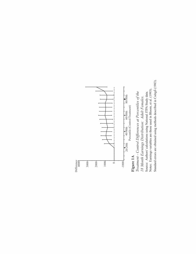
Dif
fere
nce
40
00
30
00
20
00
10
00 0
-10
00
40
/40
th6
0/6
0th
80
/80
th
Fig
ure
1A
rT
eatm
ent
- C
ontr
ol
Dif
fere
nce
s at
Per
centi
les
of
the
18 M
onth
Earn
ings
Dis
trib
uti
on:
Adult
Fem
ale
s.
Per
centi
le (
Contr
ol/
Tre
atm
ent)
20
/20
th
So
urc
e: A
uth
ors
' cal
cula
tio
ns
usi
ng
Nat
ion
al J
TPA
Stu
dy
dat
a.
No
tes:
E
arn
ing
s v
aria
ble
s ar
e th
ose
use
d i
n B
loo
m,
et a
l. (
19
93
).
Sta
nd
ard
err
ors
are
ob
tain
ed u
sin
g m
eth
od
s d
escr
ibed
in
Csö
rgÐ
(1
98
3).

Dif
fere
nce
5000
4000
3000
2000
1000 0
-1000
-2000
40
/40
th60/6
0th
80/8
0th
20/2
0th
18
Mo
nth
Ea
rnin
gs
Dis
trib
uti
on
: A
du
lt M
ale
s, F
ull
Sa
mp
le.
Per
centi
le (
Contr
ol/
Tre
atm
ent)
Fig
ure
1B
cT
reatm
ent
- C
ontr
ol
Dif
fere
nce
s at
Per
enti
les
of
the
So
urc
e: A
uth
ors
' cal
cula
tio
ns
usi
ng
Nat
ion
al J
TPA
Stu
dy
dat
a.
No
tes:
E
arn
ing
s v
aria
ble
s ar
e th
ose
use
d i
n B
loo
m,
et a
l. (
19
93
).
Sta
nd
ard
err
ors
are
ob
tain
ed u
sin
g m
eth
od
s d
escr
ibed
in
Csö
rgÐ
(1
98
3).

Heckman, Smith, and Heinrich, 56
Eligibility for JTPA
�
Awareness of JTPA
�
Application to JTPA
�
Acceptance into JTPA
�
Enrolment into JTPA
FIGURE 2
THE JTPA SELECTION PROCESS
Related Documents