NBER WORKING PAPER SERIES HOUSING SUBSIDES: EFFECTS …

NBER WORKING PAPER SERIES

HOUSING SUBSIDES: EFFECTS ON HOUSING DECISIONS,EFFICIENCY, AND EQUITY

Harvey S. Rosen

Working Paper No. 1161

NATIONAL BUREAU OF ECONOMIC RESEARCH1050 Massachusetts Avenue

Cambridge MA 02138

June 1983

This essay is to appear in A. Auerbach and M. Feldstein (eds.),Handbook of Public Economics. Part of the research was completedwhile I was a Visiting Scholar at the Hoover Institution. I would

like to thank Patric Hendershott, Michael Murray, Richard Muth, and

John Quigley for useful suggestions. The research reported here is

part of the NBER's research program in Taxation. Any opinionsexpressed are those of the author and not those of the National

Bureau of Economic Research.

NBER Working Paper #1161June 1983

Housing Subsides: Effects on Housing Decisions, Efficiency, and Equity

ABSTRACT

This paper surveys the effects of two of the most important

federal policies toward housing: the "implicit subsidy" for owner—

occupied housing in the income tax code, and the provision of housing

for low income families at rents below cost. Emphasis is placed on

the methodological problems that arise in attempts to assess the

efficiency and distributive implications of these programs.

Section 1 critically discusses the rationalization for a government

housing policy. Section 2 investigates the econometric problems associated

with estimating the effects of government policy upon housing decisions.

The federal tax treatment of owner—occupation and how it affects the

cost and demand for homeownership are discussed in Section 3. In

Section 4, the positive and normative implications of U.S. policies for

low income housing are evaluated.

The conclusion notes that the policies under concern have led to a

greater than efficient amount of housing consumption, and have on net

probably led to a more unequal distribution of income.

Harvey S. RosenDept. of EconomicsPrinceton UniversityPrinceton, NJ 08544

1. Introduction

1.1 The U. S. Housing Stock

From virtually every point of view, housing is an important commodity.

In 1979, the value of the net stock of residential capital in the United

States was over a trillion dollars, measured in 1972 dollars. (See Table

1.1.) Although it is difficult to summarize in a single measure the quality

of this stock, most experts agree that in general it is very high.1 In

1978, for example, only 3% of the housing units lacked some or all of their

plumbing facilities. Similarly, overcrowded housing which is characteristic

of many countries does not appear to be a widespread problem in the U.S.

In 1978, the median number of persons per owner—occupied unit was 2.7; for

renter occupied units the figure was 2.02. In 1970, only 7% of housing units

had more than 1.01 persons per room.3

The flow of resources into housing continues to be large. In 1980,

out of $399.00 billion spent on fixed total investment, $104.0 billion went

into the residential capital stock. (See Table 1.2.) For the past two

decades, personal consumption expenditures on housing have been between

4nine and ten percent of gross national product. For purpose of compari.son,

Table 1.3 shows the ratio of residential investment to total fixed investment

in a number of countries. The U.S. does not appear to be an outlier.

1See, for example, Aaron (1972, p. 30).

2Statistical Abstract 1980, p. 791.

Statistical Abstract 1980, p. 792. This figure is for units with allplumbing facilities, which comprised 94% of all units.

'a Statistical Abstract 1980, p. 789.

TABLE 1.1

U. S. Net Private Residential Capital Stock*

(Selected years, measured in 1972 billions of dollars)

1960 1965 1970 1975 1979

601 721 826 959 1,058

U. S. Department of Commerce, Bureau of the Census, StatisticalMstract of the United States 1980, Washington, D.C., 1980, p. 789.

TABLE 1.2

U. S. Fixed Total Investment and Residential Investment*

(Selected years, measured in current billions of dollars)

1960 1965 1970 1975 1980

FixedTotal 72.9 103.7 141.0 213.0 399.0

Investment

ResidentialInvestment 24.5 30.9 37.1 55.3 104.0

*Soce: Economic Report of the President, January 1981, p. 249.

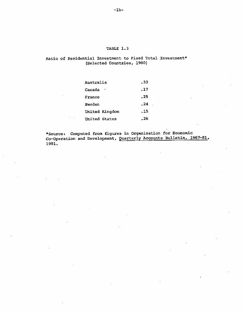
TABLE 1..3

Ratio of Residential Investment to Fixed Total Investlnent*

(Selected Countries, 1980)

Australia .33

Canada - .17

France .25

Sweden .24

United Kingdom .15

United States .26

*Soce: Computed from figures in Organization for EconomicCo—Operation and Development, Quarterly Accounts Bulletin, 1967-81,1981.

1.2 Government and Housing

The Pmerican housing market is subject to a mind boggling array of

government interventjorB by various levels of government. These include;

housing codes, which set quality standards that must be met by builders;

licensure of real estate brokers and salespeople;exclusionary zoning, which

stipulates that land in a given area can be used only for certain purposes;

open housing laws, which prohibit discrimination in the selling of housing;

rent control; interest rate and other regulations on mortgage lending institu-

tions; urban renewal programs, under which communities use their powers of

eminent domain to acquire urban land, destroy "slums," and sell the land to

private developers; real estate taxation; and interventions in the credit

market to incraase the flow of credit to housing (e.g., the Federal

Home Loan Bank Board).6

This essay focuses on what are probably the two most important federal

policies toward housing, at least in terms of costs to the government.7' The

first is not even explicitly a housing program. It consists of certainprovi—

sions of the federal income tax code which have the effect of lowering the costs

of owner—occupied housing.8

The second is the provision of housing

for low income families at rents below cost. ,Both programs subsidize

the consumption of housing, the first mostly for middle and upper income groups,

the second mostly for the poor. We will examine how each affects economic

5 The best source for an overall view of government housing p3licy remainsAaron's (1972) classic work.

6 See Congressional Budget Office (1981) for a concise description of thesemortgage programs.

7 See Aaron (1972, p. 162).

8 As noted below, there are also favorable provisions for owners of rentalhousing, but these are not very large in comparison to those of owner occupiers.

— 3_

behavior, efficiency, and the distribution of real income.

As will be seen below, a number of countries have similar policies.

Although most of our attention will be devoted to the American experience,

some international comparisons will also be made.

1.3 Rationalizations for Government Intervention

Despite the fact that housing markets tend to be fairly

competitive (see Mills (undated) ), it has been suggeted that government

action is required for reasons of efficiency as e11 as equity. Each of

these is discussed in 'turn.

1.3.1 Efficiency A±guments

The most frequently encountered efficiency argument concerns extern-

alities in housing consumption. When an individual improves his property,

it increases the value of this investment. Simultaneously, the improvement

may increase neighbors' property va1ues. However, an individual's calcula-

tion of whether or not to undertake an improvement takes into account on].y

the effect on his investments, not those of his neighbors.. Thus, the

marginal social benefits ofthe improvement exceed the private marginal ..-

costs, and the 'rational' property. owner is likely to invest less than a

socially efficient amount. .

. .

As a theoretical matter, it is hard to doubt that within a neighbor-

hood, some kind of property value interdependence exists. But it is equally

—4—

doubtful that all housing investments generate such externalities. Presunt—

ably, some such as painting outside walls create spillover effects. Others,

such as painting interior walls, do not. The usual Pigouvian analysis re-

quires that subsidies be targeted specifically at those activities that

produce the externalities. It is pretty certain that the federal subsidies

for owner-occupied housing, which in effect lower the cost of housing in

general, are inefficient.

The empirical evidence for the existence of quantitatively significant

spillovers is weak. One would expect, for example, that if externalities

were important anywhere, it would be in the slums, where housing density is

very high. Mills (undated, p. 15) notes that the presence of substantial

externalities should provide a strong incentive for single ownership of neigh-

boring dwellings in such neihborhoods. No such tendency appears to exist.

Similarly, the literature reviewed by Muth (1973, p.. 35) indicates that the

removal of slums and their replacement by public housing does not have much

of an impact upon the values of surrounding properties. To the extent &uch

effects are present, they are probably due to the community facilities asso-

ciated with the public housing (e.g., playgrounds), rather than the removal

of slum dwellings r Se.

Another externality sometimes mentioned is the "socialcost of slums."

The notion is that poor housing does more than merely lower neighborhood

property values. It breeds crime delinquency, fires, disease, mental

5

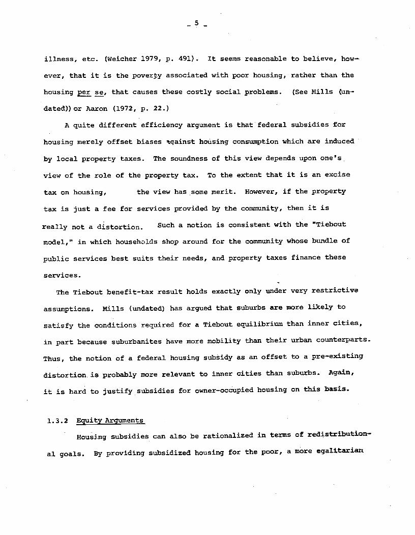
illness, etc. (Weicher 1979, P. 491). It seems reasonable to believe, how-

ever, that it is the povery associated with poor housing, rather than the

housing per se, that causes these costly social problems. (See Mills (un-

dated)) or Aaron (1972, p. 22.)

A quite different efficiency argument is that federal subsidies for

housing merely offset biases tqainst housing consumption which are induced

by local property taxes. The soundness of this view depends upon one's

view of the role of the property tax. To the extent that it is an excise

tax on housing, the view has some merit. However, if the property

tax is just a fee for services provided by the community, then it is

really not a distortion. Such a notion is consistent with the "Tiebout

model," in which househids shop around for the community whose bundle of

public services best suits their needs, and property taxes finance these

services.

The Tiebout benefit-tax result holds exactly only under very restrictive

assumptions. Mills (undated) has argued that suburbs are more likely to

satisfy the conditions required for a Tiebout equilibrium than inner cities,

in part because suburbanites have more mobility than their urban counterparts.

Thus, the notion of a federal housing subsidy as an offset to a pre-existing

distortion is probably more relevant to inner cities than suburbs. Again,

it is hard to justify subsidies for owner-occupied housing on this basis.

1.3.2 Equity Arguments

Housing subsidies can also be rationalized in terms of redistributiOn

al goals. B providing subsidized housing for the poor, a more egalitarian

—6—

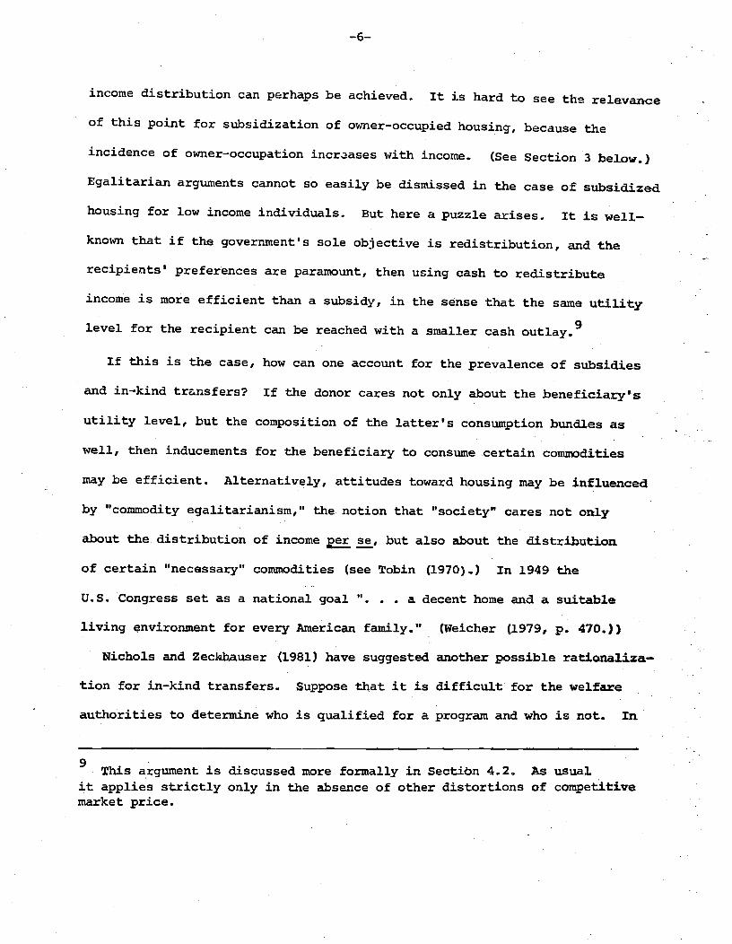
income distribution can perhaps be achieved. It is hard to see the relevance

of this point for subsidization of owner—occupied housing-, because the

incidence of owner—occupation incr3ases with income. (See Section 3 below.)

Egalitarian arguments cannot so easily be dismissed in the case of subsidized

housing for low income individuals. But here a puzzle arises. It is well—

known that if the government's sole objective is redistribution, and the

recipients' preferences are paramount, then using cash to redistribute

income is more efficient than a subsidy, in the sense that the same utility

level for the recipient can be reached with a smaller cash outlay.9

If this is the case, how can one account for the prevalence of subsidies

and in—kind transfers? If the donor cares not only about the beneficiary's

utility level, but the composition of the latter's consumption bundles as

well, then inducements for the beneficiary to consume certain commodities

may be efficient. Alternatively, attitudes toward housing may be influenced

by "commodity egalitarianism," the notion that "society" cares not only

about the distribution of income per se, but also about the distribution

of certain "necessary" commodities (see Tobin (1970).) In 1949 the

U.S. Congress set as a national goal ". . . a decent home and a suitable

living environment for every ?nierican family." (Weicher (1979, p. 470.))

Nichols and Zecl4thauser (1981) have suggested another possible rationaliza-

tion for in-kind transfers. Suppose that it is difficult for the welfare

authorities to determine who is qualified for a program and who is not. In

mis argument is discussed more formally in SectiOn 4.2. As usualit applies strictly only in the absence of other distortions of competitivemarket price.

—7—

other words, "welfare fraud" is a possibility. In the Nichols—Zeckhauser

model, in—kind transfers of inferior goods may discourage some impostors

from applying for welfare. By forcing the "truly needy" to consume a

certain bundle, consumption efficiency is reduced. But program efficiency

increases, because the money is better targeted. The optimal design of

transfer packages requires taking both kinds of efficiency into account.

It is hard to know how important any of these considerations are in

determing policy. Perhaps it is the high visibility of housing that

leads people to view it as a "problem" that must be dealt with publicly.

In any event, many economists find public policies based upon such pater-

nalistic principles to be quite unattractive from a philosophical view-

point, Indeed, Mills (undated) has suggested that in the U.S., official

paternalism toward low income groups may be tinged with racism —— the poor

are disproportionately black, and th.ere is an underlying expectation that

they cannot be expected to manage their lives without help.

Another explanation for the existence of low income housing subsidies

is political. An in-kind subsidy tends to help not only the beneficiary,

but also the producers of the favored commodity. Thus, a transfer program

that increases the demand for housing will tend to benefit the building

industry, which will then lend its support to a coalition in favor of the

program. As indicated in Section 4.1 below, housing programs for the poor

have focused on the construction of new units, thus benefitting the housing

industry rather directly.

It is also important to note that unlike cash transfers, the administra-

tion of a public housing program requires substantial amounts of resources.

-8—

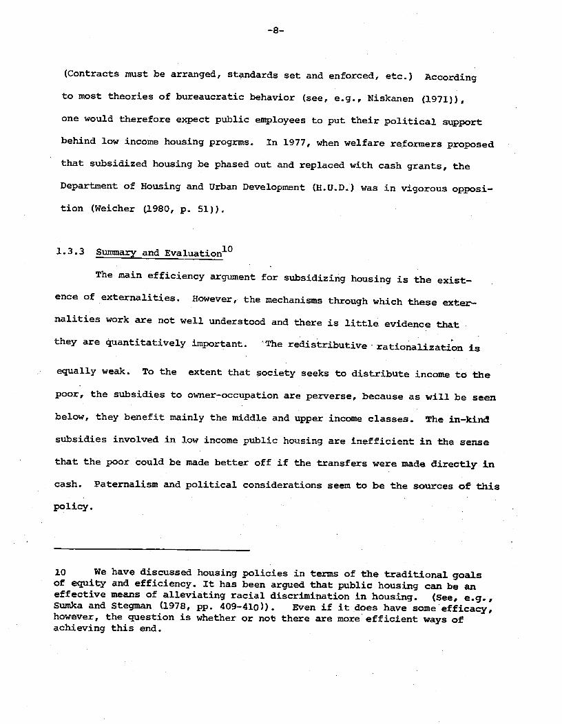
(Contracts must be arranged, standards set arid enforced, etc.) According

to most theories of bureaucratic behavior (see, e.g., Niskanen (1971)),

one would therefore expect public employees to put their political support

behind low income housing progrms. In 1977, when welfare reformers proposed

that subsidized housing be phased out and replaced with cash grants, the

Department of Housing and Urban Development (H.U.D.) was in vigorous opposi-

tion (Weicher (1980, p. 51)).

1.3.3 Summary and Evaluation10

The main efficiency argument for subsidizing housing is the exist-

ence of externalities. However, the mechanisms through which these exter-

nalities work are not well understood and there is little evidence that

they are quantitatively important. The redistributive rationalization is

equally weak. To the extent that society seeks to distribute income to the

poor, the subsidies to owner—occupation are perverse, because as will be seen

below, they benefit mainly the middle and upper income classes. The in—kind

subsidies involved in low income public housing are inefficient in the sense

that the poor could be made better off if the transfers were made directly in

cash. Paternalism and political considerations seem to be the sources of this

policy.

10 We have discussed housing policies in terms of the traditional goalsof equity and efficiency. It has been argued that public housing can be aneffective means of alleviating racial discrimination in housing. (See. e.g.,Suxnka and Stegman (1978, pp. 409-410)). Even if it does have someefficacy,however, the question is whether or not there are more efficient ways ofachieving this end.

—9—

2. Methodological Issues

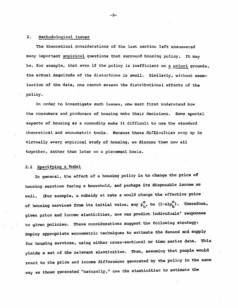
The theoretical considerations of the last section left unanswered

many important empirical questions that surround housing policy. It may

be, for example, that even if the policy is inefficient on a priori grounds,

the actual magnitude of the distortions is small. Similarly, without exam-

ination of the data, one cannot assess the distributional effects of the

policy.

In order to investigate such issues, one must first understand how

the consumers and producers of housing make their decisions. Some special

aspects of housing as a commodity make it difficult to use the standard

theoretical and econometric tools. Because these difficulties crop up in

virtually every empirical study of housing, we discuss them now all

together, rather than later on a piecemeal basis.

2.1 Specifying a Model

In general, the effect of a housing policy is to change the price of

housing services facing a household, andperhaps its disposable income as

well. (For example, a subsidy at rate s would change the effective price

0of housing services from its initial value, say h' to (l—s)p). Therefore,

given price and income elasticities, one can predict individuals' responses

to given policies. These considerations suggest the following strategy:

Employ appropriate econometric techniques to estimate the demand and supply

for housing services, using either cross—sectional or time series data. This

yields a set of the relevant elasticities. Then, assuming that people would

react to the price and income differences generated by the policy in the same

way as those generated "naturally," use the elasticities to estimate the

—10—

program's impact on behavior. We discuss problems in estimating demand

and supply functions, and then turn to the influence of the market environ-

ment upon the results.

2.1.1 Demand11

Empirical investigators typically begin by specifying a model that

relates the quantity of housing services demanded for the th observation

.(QD) , to some function f() of price income (Y.) and a vectorof demographic variables that theoretical considerations suggest mightbe relevant:

(2.1) = f(PhilYj;zj)

In some cases f (•) is specified in an ad hoc but convenient form. such

as log linear (Polinsky and Eliwood (1979)), while other times itis derived

from maximization of an explicit utility function (bbot and Ashenfelter

(l976), which is also chosen on the basis of convenience.

Equation (21) is deterministic, so the next step is to posit some

stochastic specification. Usually, an error term is appended additively.

Given a set of observations on hJ. ' hj ' Y and Z. and the1 1

stochastic specification, the model's parameters can be estimated using a

variety of econometric techniques. The behavioral elasticities implied

by the parameter estimates can then be used to predict the effects of

policy changes. Alternatively, one can obtain such predictions by sub-

stituting the new values for price and income directly into equation .1).

11For a useful survey of the results .of housing demand studies, see

Mayo (1981).

—11—

There are several problems with this standard approach:

(1) Economic theory puts very few constraints on the form of f (-),

so the investigator must make an essentially ad hoc choice with respect to

the specification of either the demand or utility function.

(2) It must be assumed that f(-) is identical across individuals.

(When time series data are used, the analogous assumption is that f(-) does

not change over time.)

(3) Demand functions like (2.1) ignore the dynamic nature of housing

decisions. Because these decisions are made in a life cycle context, expected

future prices and incomes as well as those of the current period are relevant.

(See Henderson arid lonnides (1981) or Weiss (1978).)

(4) Observations on hi are never directly observed. Only p. x ——

the value of the dwelling —- is observable.

(5) For many owner—occupiers, housing is not only a consumption item,

but an investment as well. To the extent this is the case, the theory of

portfolio behavior suggests that the demand for housing depends upon the

joint distribution of the returns from housing and other assets. Even those

econometric studies discussed below which explicitly recognize the invest-

ment nature of housing decisions have failed to take into account this

consideration.

12 Note that this need not imply that the elasticities be identical acrossindividuals; such will be the case only for the very simple Cobb—Douglas speci-fication. One can also specify a random coefficients model, which allows fora distribution of elasticities across people. See King (1980).

—12-

(6) It must be assumed that the fitted relationship will continue

to apply when a right hand side variable for a given observation changes.

For example, if an investigator using cross—sectional data finds that

3QD hi is less than one, it does not imply that increasing a particular

family's income ten percent will increase its housing consumption by a smaller

percentage. Al]. that one really learns is that in the data, poorer families

devote a larger fraction of their income to housing than richer families,

ceteris paribus. Only by assuming that poorer families would act like the

richer ones if their incomes were increased, and vice versa, can one give

any behavioral significance to elasticity estimates from regressions.

Moreover, most of the studies using cross—sectional data to examinehousing

demand implicitly or explicitly assume that all agents are in equilibrium)3

Were not this the case, then a regression of housing services on price, in-

come, and demographic variables could not be interpreted as a demand equa-

tion. On the other hand, analyses of longitudinal and time series data

often allow for the possibility that at a given point in time, households

may not be at their long-run equilbrium positions, because adjustment costs

make it prohibitively expensive to respond immediately to changes in economic

environment.

It is usually assumed that such a disequilibrium is eliminated over

time as households move gradually to their equilibrium positions (e.g., Rosen

13 An important exception is King (1980), which. is discussed below.

—13—

and Rosen (1980)). Such models lack a strong choice theoretic foundation,

but tractable alternatives are lacking. Venti and Wise (1982) measuxe-

transactions costs by including them as a random parameter in a model of

moving decisions. Their results confirm earlier conjectures that these costs

are large relative to income ($60 per month in a sample of low income house-

holds whose median monthly income was $320.)

2.1.2 Supply

A popular approach for studying the supply of housing is to assume

some housing production function, estimate its parameters, and use them to

infer the shape of the supply function.14 For example, Ingrain and Oron

(1977) assume that housing services are a constant elasticity of substi-

tution (C.E.S.) function of "quality capital" and "operation inputs" (p.284) -

Polinsky and Ellwood (1979) also posit a C.E.S. production function, but

assume that its arguments are land and capital. Follain (1979) and Poterba

(1980) eschew selection of a specific form for the production function,

and instead start by postulating supply functions that include the price

of housing and input costs as arguments. (Of course, duality considerations

suggest that one can work backward from the supply curve to the underlying

production function.)The specification of the underlying technology can sometimes pre-

determine substantive results. For example, since Polinsky and Eliwood (.1979)

14 Given the production function and input prices, one can derive themarginal cost schedule which, under competition, is the supply cuXve.

—14—

assume constant returns to scale (p. 210) the implied long run upp1y

curve of housing services is perfectly elastic, regardless of parameter

15estimates. Postulating such a technology, then, guarantees the result

that policies that affect housing demand will have no effect on the long

run producer's price of housing services, at least as long as input prices

remain unchanged. The interesting questions then become how high do prices

rise in the short run, and how much time is required to reach long run

equilibrium?

Various approaches have been used to model the process of adjust-

ment to the new equilibrium. Ingram and Oron (1977, p. 292) assume that

the most a landlord can invest each period is limited to the amount of

cash generated by the existing investment, even if this is insufficient

to close the gap between the desired and actual housing stock. Poterba

(1980) argues that the -supply of housing may be affected by conditions in

the credit market, and summarizes these by the flog of savings deposits

received by savings and loan associations. Poterba also assumes a delayed

supply response to changes in all right-hand side variables, which are

entered in polynomial distributed lags. (p. 10).

2.1.3 Market Environment

In microeconomettic studies of demand or supply, the key question

is how individual units react to exogenous changes in their budget con-

straints. No explicit consideration of the market environment is usually

taken. To understand overall effects, however, the question of market

structure is crucial -- the impact of a given housing policy will depend

15 The assumption of a horizontal supply curve is quite common, e.g.,see DeLeeuw and Stryuk (1975, p.15). Of course, to the extent that inputprices change with the size of the housing industry, the long run supplycurve will have a non—zero Slope.

-15-

upon its effect upon the market price of housing, which will in turn de-

pend mutatis mutandis upon the degree of competiveness in the market, the

amount of slack existing when the program is initiated, the extent of

housing market segmentation, etc.

The standard assumption is that competition prevails. As de Leeuw

and Struyk (1975) and Poterba (1980) note., however, even given competi—

tion, complications arise because two markets have to be equilibrated by

the price of housing services: the market for existing houses and the

market for new construction. The situation increases in complexity when

one takes into account the multiplicity of tenure modes. Each type of

housing is traded in its own submarket, and each of these (inter—related)

markets has its own clearing price. If the housing market is non—competitive,

the question of supply effects is even more difficult because of the

16absence of a generally accepted theory of price determination.

In practice, most econometric investigations of the issues discussed

in this essay ignore such considerations. As will be seen below, attention

tends to be focused upon the estimation of demand curves. It is usually

assumed that the housing market is perfectly competitive, and that the

long supply curve of housing services is infinitely elastic.17

16 An example of the use of a non—competitive framework is Rydell(1979), who attempts to explain the insensitivity of housing prices toapparent variations in market tightness by recourse to a theory of mono-polistic competition.

17 An exception is Englund and Persson (forthcoming). In their simulationmodel of the Swedish housing market, they assume that the supply of housingservices is perfectly inelastic.

—16—

2.2 Measuring Quantity and Price

Our discussion of model specification suggests that accurate

measurement of the quantity and price of housing services is crucial. This

is a very difficult task, because housing is intrinsically a multi—dimension-

al commodity —— a dwelling is characterized by its number of rooms, their

size, the quality of construction and plumbing, etc, It is therefore not

obvious how to summarize in a single number the quantity of housing

services generated by a given dwelling. Usually it is assumed that the

amount of housing services is proportional to the rent paid, or, in the

case of an owner-occupied dwelling, to the value of the house. (See, e.g.,

Polinsky and Eliwood (1979).) A problem here is that the rental value of

a dwelling at a given time may reflect characteristics of the market that

have nothing to do with the quantity of housing services actually generated.

As King (1980) points out, for example, the special income tax treatment of

rental income will generally influence market values.18

An alternative tack would be to abandon the possibility of summar-

izing housing services in a single variable, and instead to estimate a

series of demand functions for various housing attributes. An immediate

problem is the bsence of observable market prices for attributes. Recent—

ly Witte, et.al (1979) have implemented the suggestion of Rosen (1974) that

attribute demand equations be estimated in a two step process: (1) esti-

mate the implicit attribute prices from an hedonic price equation19 for

18 Other problems with the concept of housing services are discussed

by Diamond and Smith [1981).

19 A regression of the price of a commodity R on its characteristics(a vector X ) is the basis ohan hedonic price index for the commodity.The implicit price of the i characteristic is . See Rosen

L1974).

—17—

housing; and (2) use these prices as explanatory variables in regressions

with attribute quantities as the dependent variables. However, Brown and

Rosen (1.982) have shown that major statistical pitfalls are present in this

procedure, and that the validity of Witte, et al's results is therefore in,

question. Although some progress is being made in dealing with these

problems (see Quigley (1982 ), the approach that continues to predominate

is to measure the quantity of a dwelling's housing services by its market

value (if it is owner—occupied) or otherwise by its rental value.

Because the price of housing services is housing expenditures

divided by the quantity of housing services, the above noted difficulties

in measuring the latter are bound to create problems in measuring price.

Several possible solutions are found in the literature. Apopular ap-

proach is to estimate hedonic price equations for different cities, and

use them as the bases for a housing price index. However, Alexander(1975)

has pointed out several problems with this approach. One of the most

important is that the selection of a set of attributes to be included in

the hedonic price index must be decided on ad hoc grounds, but the sub—

stantive implications of the estimates often depend upon the choice made.

Further difficulties in measuring price are caused by the fact that

even within a given housing market, the price per unit of housing servi:es

may not be a constant.. Struyk et.al., (1978) have argued that one of the

key characteristics of urban housing markets is the existence of sübmarkets,

each of which has different prices per unit of housing services. (Such

differences might exist because of residential segregation.) Most empirical

studies, however, continue to assume that any given city is characterized by

a single (pre—tax) price of housing.

—18--

2.3 Measuring "Shift" Variables

In order to obtain unbiased estimates of demand and supply parameters,

one must also take into account variables other than price that might he

affecting decisions. On the demand side, probably the most obvious candi-

date is income. Standard theoretical considerations suggest that for in-

come a permanent rather than annual measure should be used. It is not ob-

vious how to compute permanent income, and investigators have dealt with

the problem in various ways. Carliner (1972) and Rosen (1979), analyzing

longitudinal data, take an average of several year's worth of annual income.

Struyk (1976) uses the fitted value of a regression of income on a set of

20personal characteristics as his permanent income measure. In time series

analyses, a distributed lag on income is often used. (See, e.g., Hendershott

and Shilling (1980).)

With respect to the selection of other shift variables, investigators

have to make arbitrary decisions with respect to which ones to choose, their

measurement, and how they interact with the other variables. Typical

candidates for inclusion are race, sex of head of household, age, number

of children, etc.

On the supply side, theory suggests that input prices are important

variables. There are serious problems involved in obtaining operational

measures of housing input costs. For example, Poterba (1980) uses the

Boeckh index of the price of inputs for a new one family structure to

.20 Neither the necessity of using a permanent income measurenor the types of solutions just mentioned are unique to the study of housing;

they appear throughout the literature on the estimation of demand functions.

measure construction costs. Although this is a commonly used index, it

is well—known that it is deficient because fixed weights are used in its

computation. Ingrain and Oron (1977) use the fuel component of the con-

sumer' s price index to account for the price of all operating inputs, but

as Rothenberg (1977) points out, it is not clear that this index captures

all the needed information.

2.4

The quandries facing students of housing are similar to those who

seek to explain other kinds of complicated economic behavior (e.g., the

determinants of business investment). Although it is easy to carp about

the siznplifications made by econometric investigators, compromises are re-

quired in order to obtain tractable models. On the other hand, in light

of the serious methodological problems, one must regard substantive con—

clusions regarding policy with a very critical eye.

3. Housing Behavior and the Federal Income Tax

In this section we discuss: (1) the key provisions of the income

tax code that pertain to housing; (2) how the provisions change the effec-tive cost of housing; (3) the impact of these cost changes upon iñdividuals

housing decisions; (4) the implications of these changes for economic

efficiency and equity; and (5) some proposals that have been made for

reform.

3.1 Housing Related Tax Provisions

Exclusion of Net Imputed Rental. The U.S. federal tax code does not

require that the net value of the services received by owner—occupants from

their homes be included as taxable income. If these same units were rented out,

—20—

the income obtained would be taxed, after deductions for taxes, interest,

maintenance, etc. In other words, because an investment in owner—occupied

housing produces in—kind income rather than cash, that income is untaxed.

Deduction of Mortgage Interest. Tax payers can deduct from taxable

income the full value of all interest payments, including the interest on

22home mortgage loans.

The deduction of interest has been a part of the

tax law since its inception. At that time (1913), however, consumer inter-

est payments were minimal.

Deduction of Local Property Taxes. Hc1necwnersaXeall0Wd.t0 deduct

all state, local and foreign taxes paid on real property. This provision,

which also dates from the beginningof the code, was based on the idea

that such taxes represent areduttiofl In disposable income. To the extent

that local taxes are user fees for locally provided services, this ration-

alization lacks validity.

Deferral of Capital Gains on Home Sales. Excluded from taxable

income are any capital gains from the sale of a principal residence when

another residence costing at least as much is purchased within two years

of the sale of the former one. Thisprovision, introduced in 1951, was a

consequence of the view that individuals' decisions to change houses were

due to personal reasons or uncontrollable circumstances, as opposed to a

profit motive. Therefore, taxation of the capital gain would cause undue

hardship.

21 For more detail, see congressional Budget Office (l981) upon which

most of this section is based.

22 There are certain limitations for interest payments on property held

for investment income, but these are not important in the current context.

For certain homeowners, it may be more advantageous to take the standard de-duction than to itemize. Sde HendershOtt and Sleinrod (1981).

—21—

One—Time Exclusion of $125,000 Capital Gains in Home Sales for

payers 55 Years of Age and Older. Provisions to shield elderly taxpayers

from potentially heavy tax burdens when they decide to become renters or

move to less costly residences were first introduced.in 1964. The cut-offage at that time was 65 years and the exemption was available only under

special circumstances. In light of this provision and the one concerning

deferral just discussed, most investigators have found it safe to assume

that for all practical purposes, the tax rate on capital gains from owner—

occupied housing is zero.

Exclusion of Income from Tax Exempt Mortgage Bonds. In 1978 states

and localities began to sell tax exempt bonds to provide mortgage funds

for owner-occupied and rental units at below market interest rates. However,

in 1980, significant limits were imposed on the issuance of new tax exempt

bonds, and issues to finance new single family housing are now banned be-

ginning in 1983.

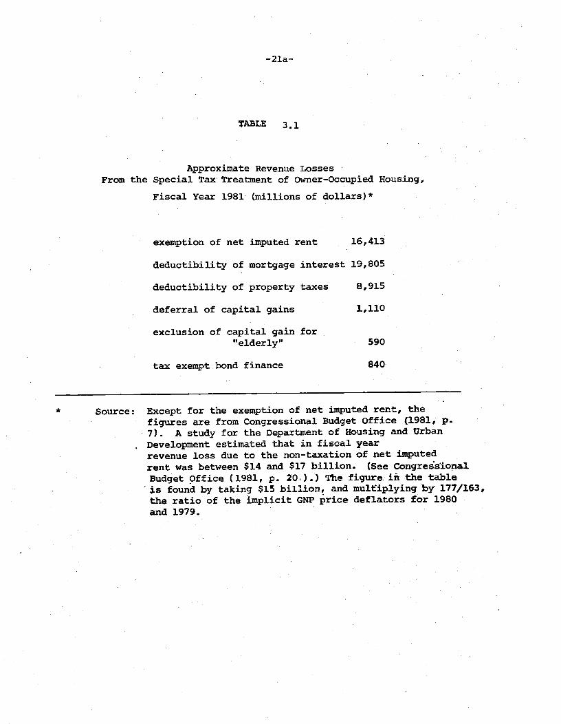
Table 3.1 shows some estimates of the foregone tax revenues

associated with the various exclusions discussed above. Note that these

estimates are based on the assumption that even if the provisions were

eliminated, people would continue to make the same housing decisions. As

both common sense and the empirical evidence reported below indicate,

this is an unrealistic assumption. Nevertheless, the figures in the table

at least indicate the orders of magnitude involved. The Congressional Budget

Office estimated that if all the tax preferences associated with housing

(except exclusion of imputed rent) were eliminated, it would be possible to

lower all personal marginal tax rates by 10% without sustaining any revenue

loss. (Congressional Budget Office 0.981, p. 40)).

-21a--

''ABLE 3.1

Approximate Revenue LossesFrom the Special Tax Treatment of Owner—Occupied Housing,

Fiscal Year 198]. (niillionsof dollars)*

exemption of net imputed rent 16,413

deductibility of mortgage interest 19,805

deductibility of property taxes 8,915

deferral of capital gains 1,110

exclusion of capital gain for"elderly" 590

tax exemptbond finance 840

* Source: Except for the exemption of net imputed rent, thefigures are from Congressional Budget Office (1981, p.7). A study for the Department of Housing and UrbanDevelopment estimated that in fiscal yearrevenue loss due to the non-taxation of net imputedrent was between $14 and $17 billion. (See CongreisionalBudget Office (1981, p. 20).) The figure. in the table

.s found by taking $15 bj1iio, and mu1ip1ying by 177/163,the ratio of the implicit GNP price deflators for 1980and1979.

—22--

The main federal tax item concerning rental housing is accelerated

depreciation. Owners of rental property may claim accelerated depreciation

on their buildings, and amortize construction period interest and real estate

taxes over a ten year period, rather than the full economic life.23 The Con-

gressional Budget Office (1981, p. 33) estimated that the foregone tax revenues

due to the tax treatxent of rental housing were about $1.9 billion. in'. 1981,

considerably less than those associated with owner—occupation.

With respect to tax concessions for housing interest payments, the

United States is roughly comparable to Western Europe. Fainstein (1980) esti-

mates that the revenue loss as a percentage of gross domestic product in the

early 1970's was about 0.3% for Germany, 0.9% for the Netherlands, 1.1% for

Sweden, 0.7% for the United Kingdom, and 0.6% for the United States. England,

like the United States, levies no tax on imputed rental income (since 1963).

On the other hand, some form of imputed net rental is taxed in Belqiun, Denmark,

Luxembourg, Netherlands, Portugal, Spain, Sweden and West'.Germany.

3.2 Effects on the, Cost of Housing

Following Aaron (1972)24 denote RG = gross imputed rent, aN = net

imputed rent, MA = maintenance, D = depreciation, T = state and local

taxes, and MI mortgage interest. Assume that io changes are ex—

23 For, a discussion of other features of the tax treatment of rentalhousing —— recapture provisions, capital gains rules and minimum tax rules—— see Hendershott and Shilling (1980).24 See also Laidler (1969).

—23—

pected in either house prices or the general price level. Then by defini-

tion

(3.1) RN=RG_MA_D_T_Mr.

If net imputed rental were subject to income taxation and a homeowner's:..

marginal tax rate were T, then the tax liability associated with home—

ownership would be t X N Under the current regime, the main ta

consequences of homeownership are to reduce taxable income by the sum of

MI and T , or alternatively, to reduce tax liability by t X (MI+T). To

find the difference between tax liabilities under the status quo and

those which would occur if net imputed rent were taxed, we simply compute

(3.2) X RN — X (MI+T)) = : T (RN+MI+T)

To get a sense for the numerical values involved, asssuine for simplicitythat the mortgage rate and the individual's opportunity cost of capital

are the same rate, i property taxes are proportion

of house value; and depreciation plus maintenance are a proportion

of house value d. Then (3.2) can be written as .T(i+t)V,

where V is the value of the house. When the homeowner spends (i+t+d)V

on housing services, he therefore derives tax savings of r(i+T)V , so

the after tax imputed rent is

(33) (i+T+d)V T(i+t)V = ((l—t)i + (l—r)r 4 diV

—24--

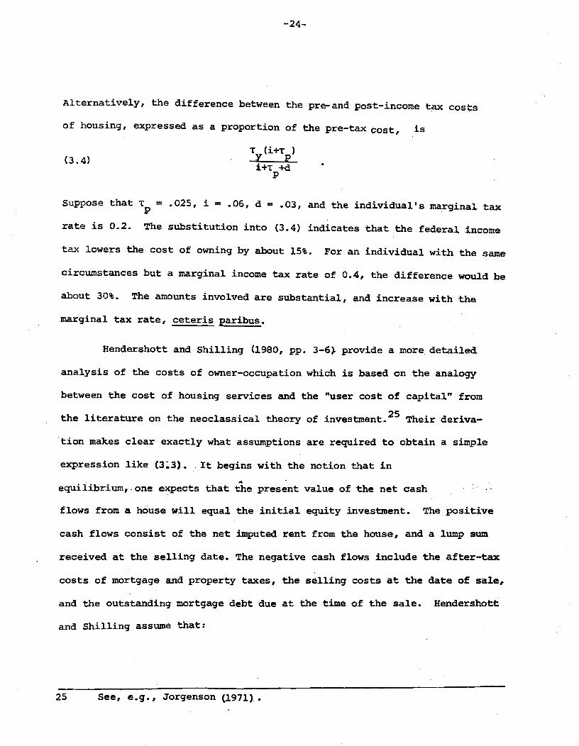
Alternatively, the difference between the pre-and post—income tax costsof housing, expressed as a proportion of the pre-tax cost, is

r (i+t(34) __y p

i+T+dp

Suppose that = .025, i = .06, d = .03, arid the individual's marginal tax

rate is 0.2. The substitution into (3.4) indicates that the federal income

tax lowers the cost of owning by about 15%. For an individual with the same

circumstances but a marginal income tax rate of 0.4, the difference would be

about 30%. The amounts involved are substantial, and increase with the

marginal tax rate, ceteris pribus.

Hendershott and Shilling (1980, pp. 3-6). provide a more, detailed

analysis of the costs of owner—occupation which is based on the analogy

between the cost of housing services arid the "user cost of capital" from

the literature on the neoclassical theory of investment.25 Their deriva-

tion makes clear exactly what assumptions are required to obtain a simple

expression like (3.3). It begins with the notion that in

equilibrium,.one expects that the present value of the net cash

flows from a house will equal the initial equity investment. The positive

cash flows consist of the net imputed rent from the house, and a lump sum

received at the selling date. The negative cash flows include the after—tax

costs of mortgage and property taxes, the selling costs at the date of sale,

and the outstanding mortgage debt due at the time of the sale. Hendershott

and Shilling assume that:

25 See, e.g., Jorgenson (1971).

—25—

(1) Inflation is expected to generate increases in net revenues

at rate p , and in housing prices at rate q

(ii) Physical depreciation of the house occurs at rate d -

(iii) The proportion, a , of the purchase price is financed with a

mortgage at rate i

N (l—T )t (l+q—y d).-Et=l (l+e)t

(l-p) (l+q-

(l+e)N

V = purchase price of the house, including land

e = after tax rate of return available on other investments..

= ratio of the value of the structure to the value of structure

plus land.= implicit rent during the first period

marginal income tax rate.

property tax rate.

mortgage payment in period t

mortgage loan outstanding at the end of period t

Because a is the loan to value ratio, (l-a)V is the equity investment

in the house. The sums on the right hand side are the present values of

N periods, at which(iv) The house is expected to be sold after

time a percentage realtor's fee, p , is paid.

Then the equilibrium condition is

N (l+p-y d)tlR(l-a)V = E

t=l (l+e)

N TiLti- E +Et=l (l+e) t=l (l+e)

(3.5)

where

R

ty=

tp=Ct =

=

—26—

the stream of imputed rents, the after tax cost of property taxes, themortgage payments, the tax savings from interest reductions, arid the

net "profit" from selling the house. Note that the income tax rate is

not included in the last term. This reflects the realistic approximation

that the rate on housing capital gains is zero.

Hendershott and Shilling go on to show that if: (i) The mortgage i5

a standard fixed rate, fixed payment mortgage or f the variable rate is

expected to remain at the constant value i through period N; (ii) Theholding period is "large" (N approaches infinity); (iii) There are no

selling costs, (p = O)j (iv) The net mortgage rate equals the net rate

of return available on other iivesthents (e= (l-t) i); (v) The expected

rate of increase in implicit rents equals the expected rate of increase in

housing prices (p=q); and (vi) The structure to value ratio is 10; then

0.6) E(l—T,)i — q + d + (l—r)tJ!

where P is the general price level.

The crucial difference between (36) and (3.3) is the presence of

q , the expected rate of increase in housing prices. When homeowners ex-

pect capital gains, it lowers their effective cost of housing. This tact

is often ignored in popular discussions of housing markets. The expecta-

tion of rising prices is an incentive to buy a house provided that

households are not constrained in their ability to borrow in the capital

markets.

The fact that housing capital gains are untaxed is reflected by the

fact that q is not multiplied by U—t7) . As a result, the decrease In

—27--

the cost of housing as the inflation rises is greater for individuals with

high values of To see this, assume for simplicity that increases in

the inflation rate are matched by increases in the nominal interest rate,

i. e., = 1 . Then taking the derivative of (3.6) with respect to q

yields

• Ty

Clearly, even if nominal interest rates increase on less than a one—for—one

basis with inflation, the tax advantages associated with the deduction of

nominal interest payments will still be greater the higher the tax rate,

though the magnitude will be less.

Hendershott and Shilling evaluate (3.5) on a quarterly basis from

1955 through 1979. As usual, some arbitrary decisions have to be made to

estimate expected inflation rates. They compute the general expected in-

flation rate as a 16 quarter distributed lag on current and past rates

of change in prices. In Table 3.2 we present annual averages of

Hendershott and Shillings' quarterly figures. The first column is based

upon a marginal income tax rate of 0.30; the second of 0.45. The figures

make clear that the cost of owner occupation fell dramatically in the 1970's,

a phenomenon due largely to increases in the inflation rate. 26 also

that the higher marginal tax rate is associated with a low user cost, as

expected.

As Hendershott and Shilling note, even this relatively elaborate.

estimate of the user cost of capital suffers from inadequacies. For example,

26 Presumably, if Hendershott and Shilling had used each year's averagevalue of r , rather than keeping it constant over time, an even greaterdecline wouYd have been evident, given that inflation was pushing peopleinto higher personal income tax brackets. See Hendershott and Slemrod (1981)for a discussion of the problems involved in computing the marginal taxrate relevant for hoineownership decisions.

-27a--

TABLE 3.2

User Cost of Housing: 1955_1979*

Owner-Occupied Rentalt =.30 t =.45y yYear

1955 .0563 .0478 .0873

56 .0500 .0410 .0803

57 .0539 .0446 .0827

58 .0591 .0502 .0878

59 .0627 .0536 .0921

1960 .0666 .0572 .0989

61 .0680 .0589 .1010

62 .0666 .0576 .0992

63 .0671 .0584 .0988

64 .0650 .0563 .0975

65 .0596 .0508 .0936

66 .0552 .0460 .0907

67 .0514 .0418 .0859

68 .0455 .0355 .0801

69 .0402 .0291 .0786

1970 .0492 .0378 .0927

71 .0419 .0313 .0809

72 .o4ri .0299 .0818

73 .0369 .0250 .0866

74 .0350 .0223 .0866

75 .0241 ,0117 .0681

76 .0292 .0165 .0801

77 .0227 .0093 .0807

78 .0177 .0040 .0847

79 .0231 .0059 .0867

*Source: Averages of quarterly figures presented by Hendershott andshilling (1980, pp. 33—34).

—28—

it does not take into account people's expectations on the future course

of tax policy. Neither does it allow for the holding period or deprecia-tion rate to vary with the tax structure. Similar problems, of course,

S

have been encountered in attempts to estimate the after tax costs of

business capital.

Hendershott and Schilling use a - similar framework to derive -.- -

the user cost of rental occupation. (The equilibrium condition takes into

account the federal tax provisions for rental housing.) Their calculationsare reported in the third column of Table 3.2. Over time, renting has become

expensive relative to owning. The implications of this phenomenon are dis-cussed below.

It is common to refer to the tax induced lowering of the relative

cost of owner—occupation as an "implicit subsidy" of owner—occupied housing..

Alternatively, housing related deductions are viewed as "tax expenditures",

items that are exempt from tax but which would be included under a compre-

hensive tax base. Although we follow this practice, it should be noted

that some object to it strenuously. First of all, in order to characterize

an item as being "exempt", one must first have some kind of criterion for

deciding what "ought" to be included. As is well known, there exists no

rigorous set of principles for determining what belongs in income.

(Musgrave (1959)).

In addition, the tax expenditure concept has been attacked on more

philosophical grounds:

"...The tax expenditure concept implies that all incomebelongs of right to the government, and that what

government decides, by exemption on qualification, notto collect in taxes constitutes a subsidy. Thisviolates a widely held conviction, basic to the Americanpolity...that the income earned by the people belongs to

them, not the government." (Jones, (1978, p. 53) ) -

—29—

Characterizing the tax provision discussed herein as a "subsidy" is not

meant to carry these ideological implications, but merely to describe their

impact on the cost of owner-occupation.

3.3 Effects on Behavior

3.3.1 Housing Decisions

Laid].er's (1969) early attempt to assess the impact of the federal tax

treatment of housing upon housing decisions begins with an estimate of its

effect upon the cost of housing for each of several income groups. This is

done by evaluating expression (3.4) with reasonable values of the appropriate

parameters. (All parameters except the marginal tax rate are constant across

income groups.) To find the amount of housing demand generated by these tax

induced price changes, Laidler assjmes a price elasticity of demand of -1.5,a figure consistent with much of the econometric literature completed at the

time of his study. He finds that in 1960, the housing stock of $355,369

million dollars would have been $60,699 million smaller had imputed rent been

taxed.27 This calculation assumes that the long run supply of housing services

is perfectly elastic, an assumption that is in line with some econometric

evidence.

One problem with the Laidler estimates is that the price elasticity

used is based upon econometric studies which ignore the impact of taxes

upon the relative price of housing. In addition, attention is focused

only upon the quantity of housing consumed by owner-occupiers, with no

attempt made to incorporate the effect of taxes upon the tenure choice.

Subsequent work has attempted to remedy these problems.

27 Laidler £1969, p. 60).

—30—

Rosen L979) uses cross-sectional U.S. data from 1970 to estimate

jointly equations for the quantity of housing services demanded and the tenure

choice. He assumes that the demand for housing services by owners (conditional

upon owning) is a translog function in the relative prices of owner—occupied

housing and permanent income, with an intercept which depends upon the

individual's personal characteristics.28 The price of owner—occupied housing

is based upon equation (3.3). A probit equation is used to model the choice

between renting and owning. The choice depends upon the relative prices of

both owner and renter-occupied housing, permanent income, and the same set of

demographic variables as in the demand function. The two equations axe. estimated

using a statistical procedure which corrects for possible biases associated

with the fact that the assortment of people into tenure modes in not random.

(Heckman (1979).)

The results indicate that the price elasticity of demand for owner—

occupied housing services evaluated at the mean is —1.0; the income elasticity,

about 0.76.29 The sign of the price-income interaction term is positive,

implying that the price elasticity of demand falls with income. The effective

price of owner—occupied housing also enters the tenure choice equation with a

negative sign, while income affects the probability of owning positively.

28 These include age of head of household, number of dependents under

-

age 17 in the family unit and age and sex of head of household. Permanentincome is a four year average of annual income.

29 McRae and Turner (1981) argue that allowing for the impact of taxes uponf actor input ratios in the production of owner-occupied housing would lead to alower estimates of the income elasticity of demand. Unfortunately, .they study only purchasers of homes with mortgages from the Federal HousingAaniinistration (FHA), a rather unrepresentative sample.

—31--

The parameter estimates are used to predict how housing decisions

would change if net imputed rent were taxable. Such a change would gener-

ate a new value of the price of owning for each family. 30(Assuming that

the long run supply curve of housing services is perfectly elastic, the

possibility of changes in the pre-tax price of housing services can be

ignored.) By substituting these new values into the probit equation, the

expected proportion of homeowners under the new regime can be calculated.

Similarly, by substituting into the demand equation, the expected amount

of housing demanded condithnal on owning can be predicted.

The results are shown in Table 3 .3. Taxation of net imputed rent

produces substantial reductions in the expected amount of owner—occupied

housing demanded. Although families in the highest income brackets face

greater increases in the price of housing, their demand is sufficiently

less price elastic that their demands actually fall by smaller amounts.

The third column shows how the expected percentage of homeowners decreases

due to the removal of the tax advantages. The average change in the inci-

dence of owner—occupied housing for the entire sample is 4.4%. In another

simulation, Rosen assum that the removal of the housing tax subsidy is

accompanied by a proportional reduction in marginal tax rates so as to keep

tax revenues constant. Despite the income effects so generated, ther are

still sizeable decreases in the quantity of housing demanded and in the

percentage of homeowners in each income bracket.

30 Specifically, the price of a unit of housing services would rise from

$1 — T(l+.r) (see equation 3.4) to $1.

l+t+d

—32—

TABLE 3,3

The Effects of Taxing Net imputed Income Upon Housing Decisions (1970)*

Status Quo Change in Change inGross Income Group House Value House Value % Owning

0— 4000 10991 —1254 —2.6

4— 8000 14022 —2549 —3.9

8—12000 17856 —3107 —4.7

12—16000 21134 —3756 —4.9

16—20000 26665 —4343 —5.0

20—24000 29893 —4879 —5.4

24—28000 36477 —4379 —5.1.

>28000 48031 —4250 —4.8

*Source: Rosen (1979).

—33..

King (1980) studies the impact of taxes on housing decision in the

United Kingdom, where, as noted in Section 3.1, the tax treatment of housing

is similar to that of the United States. Like Rosen (1979), he examines

both the tenure choice and the quantity of services demanded conditionalon

that choice. In Rosen's analysis the two decisions are modelled in an ad

hoc fashion, so that there is no guarantee that the estimates are consistent

with a single underlying utility function. In contrast, King derives both.

equations from the same structure of preferences.

Another important feature of King's model is that it allows for the

possibility that there is rationing in the choice of tenure modes. In the

United Kingdom, essentially three types of dwellings are available; owner—

occupied, government subsidized rental, and unsubsidized furnished rental.

Mortgages are not freely available in the U.K., and are rationed among

applicants. In addition, admission to the subsidized rental sector is

also rationed. King assumes that the household chooses the unsubsidized —

rental sector only if it is rationed out of the other two.

In King's model, preferences are represented by a homothetic transiog

indirect utility function,

2(3.7) in v. = in (L.._) — —2 (2)g]. gi gi

where V. is the th individual's utility, y. is income hi is the

price of housing services (which is defined using an expression like (3.4)),

Pgjis a price index for all other goods, and the B 's are the utility

function parameters. On the basis of a suitable stochastic specification,

King eomputes the probability that each individual will be observed in a

given tenure' mode as a finction of the utility

function parameters, and hence is able to deduce the likelihood function.

The 's are then estimated by maximum likelihood.

—34—

An unusual aspect of King's model is that he does not include any

controls for the demographic situation of the family, as is common in

most housing demand studies. Income and the relative price of housing

are the only explanatory variables. King does assume a "random coeffjcj"model, i.e., that and2 are to be regarded as means of the relevantdistributions.

King estimates the model with cross sectional

data from..1973-74 for England and Wales. - He finds

(s.e.=.0008) and 2O.0238 (s.e.=.0009). Perhaps more useful are the

implied price elasticities of demand for housing. Evaluated at the means,the price elasticity of demand for owner—occupied housing is —.523; for

subsidized rental, -0.498; and for furnished rental, —0.645. (p.156.)

This elasticity for owner-occupation is somewhat less than Rosen's (i979).figure of about —1.0 for U.S. data. King's analysis does not provide an

estimate of the income elasticity, because a value of 1 is imposed by the

utility function (3.7).

A disturbing aspect of King's results is that a statistical test

of the hypothesis that the utility functions for the discrete and continu-

ous choices are identical is rejected at conventional significance levels.

He suggest two explanations for this finding. One is that different

spouses are responsible for different parts of the decision, and the two

spouses may have different utility functions. The second is that the as-

sumption that rationing probabilities are exogenous results in a serious

model misspecification. Presumably, this latter deficiency could be

corrected by making the rationing probability a function of some observ-

able demographic chracteristics. But it is hard to imagine how to specify

—35—

a set of characteristics that would affect the probability ofrationing

but not affect the decisions themselves.

In another paper, King (198].) uses his estimates to predict the

consequences of taxing the imputed income from owner-occupation.31 Under

the assumption that the increased tax revenues are distributed as a flat

rate lump sum amount to each family, he finds that the taxation of net

imputed rent leads to an overall decline in the lOng—run consumption of

housing services of 13.7%. This is not too different frn Rosen's re—

suits for the U.S.

In the exercise just described, King makes the "standard" asstmtp—

tion of an infinitely elastic supply of housing services. He also does

the simulation assuming..a priäe elasticity of-supply of 2.0,

a value found by Poterba (1980) in U.S. data. In this case, the overall

average percentage decrease in housing consumption is 12.2%. Thiá is

less than the result obtained in the perfectly elastic case, because

part of the removal of the subsidy is offset by a lower pre—tax price. It

is interesting to note that departing from the assumption of perfectly

elastic supply does not have a dramatic impact on the substantive results.The studies discussed so far have ignored the impact of (non-taxable)

expected capital gains upon housing decisions. This omission is probably

a consequence of the fact that cross—sectional data are not well suited for

dealing with, such a phenomenon. Rosen and Rosen (1980) use U.S. time series

data to study the determinants of the choice between renting and homeowner—

0 enoUS to the31 I these calculations, the tenure choice is assumed to be ex g

model.

—36-

ship. In their model, it is assumed that the overall proportion of families

who desire to be owners in a given year depends upon relative price of home-

owning to renting, per capita permanent income, and a vector of shift vari-

ables. They posit a simple partial adjustment model to account for the fact

that in a given year, the actual number of homeowners will not necssariiy

equal the number who desire to own.

The expression for the price of owner—occupied housing used by Rosen

and Rosen is essentially expression (3.6). The expected capital gains

component of the expression is calculated as the difference between the

one—year forward preduction of house value, , and the current value:ti-i

Vt = - V. An ARIMA model with one autoregressive and one moving

average parameter is used to generate The price of renting is

simply the rental component of the consumer price index.

The relative price of owning to renting is entered as a polynomial

distributed lag, and permanent income is "proxied" by consumption. To take

account of the possibility that credit rationing may affect people's abil-

ities to become homeowners, a variable measuriig the availability of

deposits at th±ift institutions is also included.

The model is estimated using annual U •S. data fqr the period 194974.

The price term.is negative and significant..at.conventioziái levels.

The coefficient on income is positive and also significant. There is no

strong theoretical presumption for a positive effect of real par capita

permanent income on the incidence of homeownership, but it crops up

virtually every study. The avaLiability of funds at credit institutions

exerts a positive effect on the proportion of homeowners, but this coeffi-

cient is not estimated precisely.

—37—

To assess the quantitate implications of their results, Rosen and

Rosen use them to predict the long—run consequences of changing the tax

treatment of housing. More specifically, the price of owner—occupied

housing that would prevail in the absence of tax preferences

is substituted into the regression and the long-run proption ..of home

owners calculated. The model predicts a change in the incidence of owning

from 64% to 60% of all households in 1974. Because the income tax provi-

sions relating to homeownership only became important with the rise in

marginal tax rates associated with World War II, this implies that about

one—fourth of the 16% increase in homeownership between 1945 arid 1974 carl

be attributed to these tax factors.

In another time series analysis of the tenure choice in the U.S.,

Hendershott and Shilling (1980) study quarterly changes in an "adjusted

homeownership rate," i.e., an ownership rate adjusted for changes in the

demographic structure of the population. The relative cost of owning to

renting and real disposable income per capita are the key explantoxyvariables. The costs of the two housing modes are computed as discussed in

Section 3.2 (see the text surrounding Table 3.2). Both variables are entere

in third degree polynomial lags.

Estimating the model with quarterly data for the period 1960.2

to 1978.4, Hendershott and Shilling find a tatistica1ly significantresponse to changes in the relative costs of owning and renting. Long

lags appear to be present; the peak response takes place after 12 to 15

quarters (p.26). Income has a positive and statistically significanteffect on homeownership only when the user cost is based upon a tax rate

of 0.30.

—38—

The regression coefficients are used to predict what the long—run

homeownership rate would have been in 1974 if property taxes and interest

payments had not been deductible. Hendershott and Shilling estimate that

the incidence of homeownership would have been 59% conditional on the

average marginal incothe tax rate being 15%, and 57.5% conditional on a -

Value of 30%. It is striking to note the similarity to the result of

Rosen and Rosen, despite the differences n model specification and defin—.

ition of the price of housing services.

3.3.2 Investment Decisions

The models discussed above view housing primarily as a consumption

good, albeit one whose analysis is particularly complicated because of its

durable nature. In addition, housing is a form of investment, and as

such., it competes with other assets for a place in people's portfolios.

(See, e.g., Henderson and loannides (1981).) Thi aspect of housing has re-

cently received considerable attention in discussions of whether invesment

jn housing4 has crowded out investment in business capital, and hence contrib-

uted to the "productivity crisis." -

tpirical resolution of this issue would require joint specification and

estimation of housing and physical plant and equipment equations. tjnfortun—

ately, e.ven after several decades of careful research on the determinants of

business investment, not much consensus with respect to how the process-

should be modelled has developed. (See, e.g., Sunley (1981). We discuss,

then, a few theoretical and:empirical studies whose results are indicative of

what might be happening, but are certainly not demonstrative.

—39—

To begin, it is important to note the asymmetry in the tax treatment

of owner—occupied housing and business investments during inflationary

periods. It is sometimes argued that the key to the difference is the fe.ct

that owner-occupiers are allowed to deduct nominal rather than real mortgage

interest. However, as Summers (1380) points out, this is somewhat misleading

reasoning, because nominal interest payments are also deductible on loans

taken out to finance other types of investment. Thus, deductibility sedoes not increase the attractiveness of owner-occupied housing vis a vis

other forms of investment.32 The important sources of asymmetry are that:

(1) In the presence of inflation, depreciation of business investment based

on historical costs lowers the real value of depreciation allow'ances33 and.

(2) Owners of physical capital pay tax on nominal rather than real capital

gains. Other things being the same, then, increases in inflation increase

the effective tax rate on business capital. Thus, inflation raises the

relative cost of an investment in business capita]. to one in owner-occupied

housing. When this fact is built into theoretical models which determine

the amounts of residential and business investment, the result is predictable

——with reasonable parameter values, when inflation increases, the amount of

owner—occupied housing relative to business investment goes up. (See

Hendershott and Ku (1981), Feldstein (1981 ., or Muth (1982).)

Summers (1980) notes that an implication of such theories is that in

the short run, an increase in the permanent expected rate of inflation should

32 A possible exception occtfrs if. ownership of housing relaxes capital marketconstraints that would otherwise be binding (Summers (1980, p. 2 ).

33 Note that the distorting effect of a given level of inflation canbe offset by a suitable rate of accelerated depreciation.

—40--.

increase the market price of housing and reduce the value of the stock market..

He regresses the "excess returns" of both the stock market and owner—occupi

housing on changes in the permanent expected rate of inflation. The excess

return on the stock market during a given period is defined as the ratio of

capital gains plus dividends to the beginning of period market valuation, all

minus the beginning of period treasury bill rate. The analogous measure for

housing is the appreciation in the price deflator for one—family structures

less the beginning of period treasury bill rate. (Imputed rent is ignored.)Finally, the expected inflation rate is estimated by assuming that expecta-tions are formed on the basis of an autoregressive moving average process

applied to the preceding 10 years of data on inflation.

Summers estimates the regressions with quarterly U.S.. data from 1958—

78. The results suggest a strong negative relationship of excess stock

returns to increases in the expected inflation rate. A 1% increase in the

expected inflation rate reduces the value of the stock market by 7.6%. Ift

contrast, a similar increase in inflation increases the value of a house by

1.68%. As Sunmiers emphasizes (p.11), these results do not prove that the

inflation—taxation interaction has increased residential, capital at the

expense of business capital. First of all, inflation rates and housing prices

generally have moved, together over time, while the stock market has moved in

the opposite direction. It is therefore dangerous to ascribe a structural

interpretation to such regressions. More importantly, the regressions do not

even attempt to establish a link between the price changes induced by the

inflation—taxation interaction and individuals' investment decisions.

—4].—

3.3.3 Summary and Evaluation

The federal income tax treatment of owner—occupied housing lowers the

Cost of owner-occupation relative to renting. Studies of housing demand and

tenure choice in the United States, as well as the United Kingdom (where the

relevant tax provisions are similar) suggest that these provisions have had

a substantial impact on housing decisions. They Induce people to become

homeowners, and to consume more housing conditional on owning. The interac-

tion of inflation with the tax system has exagerated these effects. Although

there is speculation that the expansion of the housing stock has come at the

expense of business capital, not much in the way of econometric evidence is

available.

Although considerable progress has been made in explaining housing

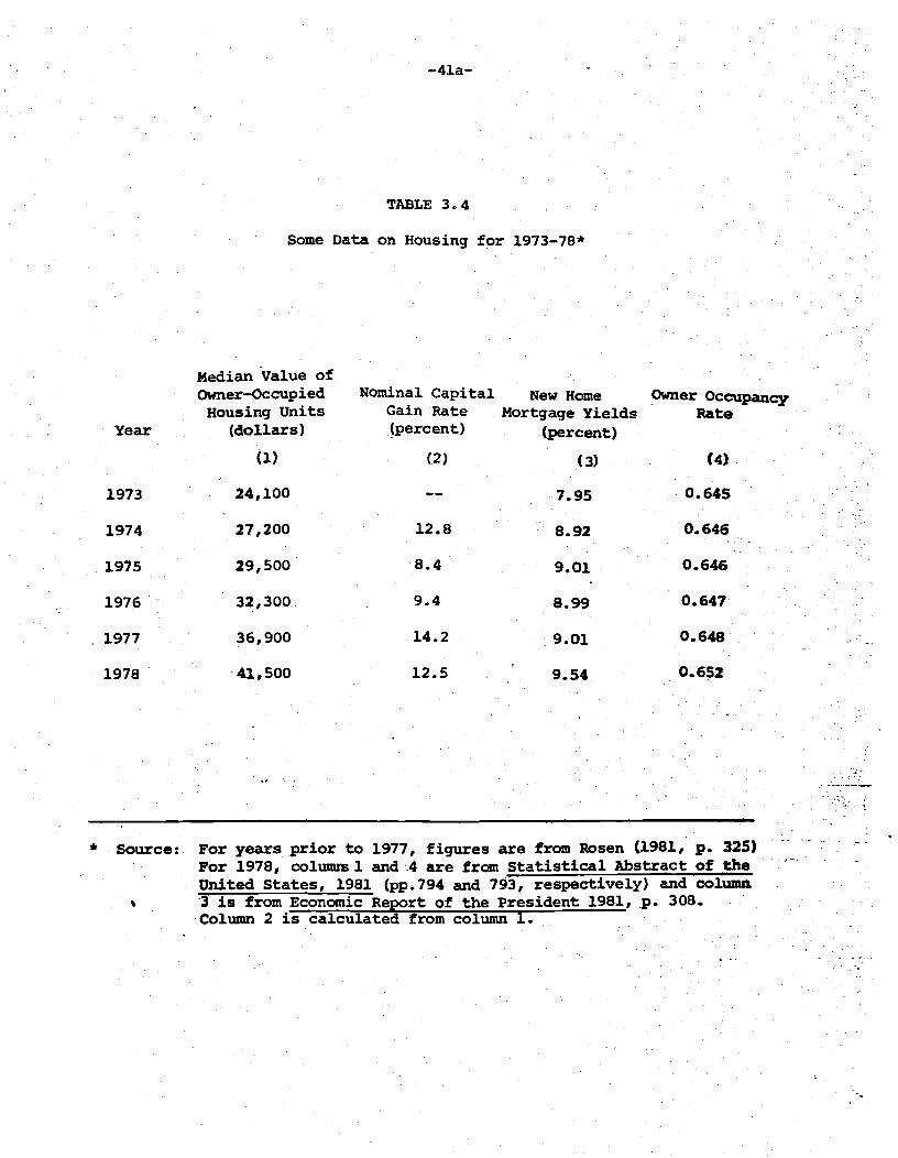
behavior, much remains to be done. Consider the figures in Table 3•434 Even

without any elaborate calculation of the user cost of housing, it is clear

from columns 2 and 3 that owner—occupied housing was a good deal in the

middle 1970's. The nominal capital gains rates tended to exceed mortgage rates.

As a very rough approximation, one could say that owner—occupiers were con-

suming "free housing" over this period. Yet column 4 indicates that there

,was hardly a rush into owner—occupation. The proportion of owner occupiers

moved from just under 0.65 to just above it.

It is not hard to come up with explanations for this phenomenon. Trans-

actions costs may inhibit the switch from renting to owning. Rationing in

the credit market may prevent individuals from obtaining loans.35 Jaffee

and Rosen (.1979) have emphasized the fact that households with different

mis discussion is based on Rosen (1981).35 This possibility is discussed by Kearl (1979).

—41a-

TABLE 34Some Data on Housing for 1973_78*

Median Value of

Owner-Occupied Nominal Capital New Home Owner OccupanHousing Units Gain Rate Mortgage Yields Rate

Year (dollars) (percent) (percent)(1) (2) (3) (4)

1973 24,100 7.95 0.645

1974 27,200 12.8 8.92 0.646

1975 29,500 8.4 9.01 0.646

1976 32,300 9.4 8.99 0.647

1977 36,900 14.2 9•oj 0.648

1978 41,500 12.5 954 0.652

* Source: For years prior to 1977, figures are from Rosen (1981, p. 325)For 1978, colunus 1 and .4 are from Statistical Abstract of theUnited States, 1981 (pp.794 and 793, respectively) and column.3 is from Economic Report of the president 1981, p. 308.Column 2 is calculated from column 1.

demographic characteristics have quite different homeownership rates, and

the proportion of the population of those groups with low rates has been

increasing.

Finally, the price figures in the table are ex post. Ex ante,

individuals do not know for sure how much and in what direction prices will

move. Presumably, housing decisions depend upon the subjective uncertainty

concerning the future course of prices. The point is that such potentiallyimportant phenomena as these have either been ignored or treated periphera].jy

in empirical studies of the impact of taxes on housing. As progress on

the theoretical and econometric issues in dealing with these problems is

made, one can expect more reliable estimates to be produced.

3.4 Efficiency and Equity Implications

For purposes of estimating efficiency effects, the basic problem is to

model the tax law in such a way that the usual techniques for measuring ex—

cess burden can be used. Laidler (1969) recognizes that the tax provisions

related to housing introduce a wedge between the effective price of housing

services and their marginal cost. Therefore, it can be analyzed like any

other distortion. In particular, assuming there are no other imperfections

in the system, and given estimates of: (a) individual i's mtr'inal taxtax rate, (b) the proportion of his housing costs which are not su1ject

to tax, , and Cc) the compensated price elasticity of demand T1., then the

size of the welfare loss 'triangle' is:36

36See Harberger (1964).

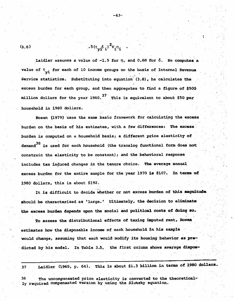
-.43—

(3.8) .5(t .&.)2V.fl.yl]. ii

Laidler assumes a value of —1.5 for r, and 0.68 for . He couputesa

value of t. for each. of 10 income groups on the basis of Internal Revenue

Service statistics. Substituting into equation (3.8), he calculates the

excess burden for each group, and then aggregates to find a figure of $500

million dollars for the year l960. This is equivalent to about $50 per

household in 1980 dollars

Rosen (1979) uses the same basic framework for calculating the excess

burden on the basis of his estimates, with. a few differences: The excess

burden is computed on a household basis, a different price elasticity of

demand38 is used for each household (the translog functional form does not

constrain the elasticity to be constant), and the behavioral response

includes tax induced changes in the tenure choice. The average annual

excess burden for the entire sample for the year 1970 is $107. In terms of

1980 dollars, this is about l92

It is difficult to decide whether or not excess burden of this magnitude

should be characterized as 'large.' Ultimately, the decision to el{m(nte

the excess burden depends upon the social and political costs of doing so.

To assess the distributional effects of taxing imputed rent, Rosen

estimates bow the disposable income of each household in his sample

would change, assuming that each would modify its housing behavior as pre-

dicted by his model. In Table 3.5, the first column shows average dispos—

37 Laidler (1969, p 64) This is about $1.3 billion in terms of 3.980 dollars.

38 The uncompsnsated price elasticity is converted to the theoretical-ly required compensated version by using the Slutsky equation.

-43a—

TABLE 3.5

Disposable Income Under Alternative Tax Treatment of Net Imputed Rent*(1970)

(1) (2) (3)Status Quo Tax Net Imputed Tax Net Imputed

Rent Rent and MaintainIncome Group Constant Tax Revenues$ 0 — 4,000 $ 2686 $ 2666 $ 2675

4 — 8,000 6024 5953 6018

8 —12,000 9452 9317 9678

12 —16,000 12715 12465 12736

16 — 20,000 15829 15396 3.5795

20 — 24,000 19088 1852]. 19086

24 — 28,000 22248 21482 22208

> 28,000 30306 28800 30186

* Source: Rosen (1979, p.20).

—44—

able income for each income group under the status g. Column 2 shows

disposable income if net imputed rent is taxed, and the government makes no

other adjustments in the tax schedule. Column 3 is based on the assumption

that marginal tax rates are adjusted proportionately so as to keep tax revenues

the same as they were under the status quo. As is well-known, it is impossible

to summarize the degree of inequality in any "objective" distributional

measure. (Atkinson (1970)). In any case, it appeazs that the taxation of

net imputed rent would tend to distribute income away from high income

groups, although at the very bottom end of the scale disposable incomes

would fall by small amounts.

King t1981) uses his estimates of housing demand parameters in the

United Kingdom to assess the efficiency and distributional consequences of

the tax treatment of housing in that country. Instead of relying upon the

usual second order approximation, he estimates the welfare effects directly

using the utility function (3.7). Specifically, King computes each house-

hold's "equivalent gain" (EG), the sum of money which it would have accepted

under the status quo as equivalent to the impact of taxing the imputed

.thrental from owner-occupation (pp.8-9). The equivalent gain for the i.

individual can be defined algebraically in temns of the indirect utility

function:

11Vj(Y+EGjPji.Pg) Vi(YiPh+iPg)

a

where the super'ipts- 0 and ldenote values under the status g and the

new regime, respectively, and the other variables are as defined above. King

—45--

observes that for a tax reform that holds tax revenues constant, the sum. of

the cjuiv2.lait giin 2rovides a measure of the efficienc-r gain to the

econoiiy. Given c:ntant revenues, a positive average EG "...is equivalent

to a Pareto—improvement combined with. a set of lump-sum redistribut_jan

among households." (p.9.)

For the sake of contrast, King also computes for each household a "cash

gain" (CG), which is just the effect of the reform on the household's cashflow on the assumption that its behavior is exogenous (p.7). A comparison

of EG and CG indicates whether or not allowing for endogenous housingdecisions has important Substantive consequences.

Table 3.6 shows the distribution of gains and losses by income decile

for both measuxes. The reduction in excess burden, which is given by the

- overall-, mean value of the equivalent gain, is O.l7 per week, about

0.4 of one percent of mean income. The overall' value of the cash gain has

to be zero given that it is computed under the assumptions of exogenous

behavior and constant tax revenues. The figures indicate that just as mT

the U.S., non-taxation of net imputed rent has substantial distributionalintplications.9Those with higher incomes would tend to be made worse off

by the taxation of net imputed rent, and vice versa. -

Of course, the estimates of efficiency and equity effects describedin this section can be only as good as the underlying behavioral estimates,

so all the caveats of Section 2 should be recalled. In addition, several.

other qualifications deserve attention:

39 Patric Hendershott has pointed out to me that comparison of Icing's-results with those of Rosen for the U.S. (Table 3.5) must take intoaccount the fact that Rosen assumes tax revenues are held constant viaproportional changes in marginal tax rates, while King assumes a lumpsum rebate.

-45a-

TABLE 3.6

Gains and Losses from Taxing Imputed Rent in the United Kingdoxn*

C-per week, 1973 prices)

Decile Mean Income Mean CG Mean EG

1 10.77 .52 0.76

2 17.13 .34 0.67

3 24.34 .28 0.58

4 31.39 .24 0.48

5 37..64 .13 : 0.36

6 43.65 .05 0.24

7 49.43 —.05 0.14

8 57.07 —.24 —0.09

9 67.64 —.40 —0.32

10 103.20 —.87 —1.15

Overall 44.23' 0 0.17

*$ojt.ce: King (1981, p. 41).

—46—

1. The results all involve comparison of long—run equilibria. The

short—run capital gains and losses in housing which might occur between

equilibrium positions could have important distributional consequences.

2. The studies focus on housing as a use of income. Presumably,

if there were major decreases in the demand for housing, it would have a

large effect on the seurces side of the account as well. The owners of those

factors used intensively in the production of housing services would suffer

reductions in income. As of yet, such effects have not been integrated into

studies of the distributive aspects of the tax treatment of housing.

3.5 Proposals for Reform

In the absence of clearly articulated goals for U.S. housing policy,

it is bound to be difficult to determine how the tax treatment of housing

should be changed. If we discount the externality arguments of Section 2,

then it would appear that subsidizing owner-occupation is inefficient. More-

over, if we take the evidence on the distributional implications from Section 3.4

seriously, this inefficiency cannot be viewed as "buying" society more equality.

Such considerations have lead a number of investigators to suggest that net

imputed income should be taxed at the same rate as other sources of income.

Thus, for example, Hughes (1980) argues that "...the inclusion of imputed

housing income in taxable income would be justified under almost any consistent

income tax system." (p.74) From this point of view, the only valid reason for

not taxing imputed rent would be administrative difficulties involved in

computing it.

—47--

This argument is in line with the famous Haig-Simons principle of tax

design, which states that an individual should pay tax on his total income

regardless of the source. It is often suggested that departures from the

Haig—Simons criterion necessarily induce inefficiencies. Clearly, the excess

burdens reported in the last section are non-trivial. But the excess burden

computation is implicitly based upon a comparison with a lump sum tax. In

practice, such taxes are infeasible. The theory of optimal taxation shows

that if lump sum taxes are excluded, the efficiency maximizing set of tax

rates is in general a complicated function of the elasticities of demand and

supply for all commodities. (See Sandmo (1976)). It is only in very special

cases that one would expect efficiency to require equal rates for all sources

of income. On the other hand, it is also highly improbably that the efficient

tax rate on imputed rental income is zero. Determination of the appropate

rate has received some attention (e.g., Atkinson (1977)), but remains an

important topic for future research.

A number of reform suggestions have been made which maintain the

basic structure of the status , but seek to ameliorate its inegalitarian

income distributional consequences. Such a view might be consistent with

the notion that there is some merit to the externality argument, but that

the subsidy goes too far in helping high income groups. Alternatively,

one might believe that there i5 no valid externality argument, but that it

is politically and administratively impossible to include imputed rent in

the tax base. In any case, these reforms focus upon reducing the valne of

mortgage interest and property tax deductions to upper income individuals.

One possibility would be to put ceilings on the amounts of mortgage inter-

est and property tax deductions, and/or capital gains exclusions. Other

—48—

proposals would convert the deductions into credi——every homeowner would

be allowed to subtract some proportion of interest and property tax pay-

ments from his tax liability. In this way, those with higher marginal tax

rates would not enjoy an advantage, ceteris paribus.

Questions of administrative feasibility lessen the attractiveness of

deduction limitations. Unless limitations in the deductibility of mortgage

interest were accompanied by a ceiling on all interest deductions, taxpayers

could simply secure mortgage loans to other assets. More generally, it is

difficult to evaluate such. proposals because it is not clear what their

objectives are, and what other policy instruments are assumed to be available.

If increased efficiency is the goal, why not tax imputed rent at the appropri-

ate rate? If more income distribution is sought, why not increase marginal

tax rates at upper income levels?

So far, our discussion of the equity implications of the tax treatment

of housing has focused on distribution of income between upper and lower income

groups. A number of observers have urged reform because the status

violates horizontal equity, the injunction that equals be treated equally for

purposes of tax policy. If there are two identical people, but one owns and.

one rents, the renter does not obtain the tax advantages of owning.40 A

possible solution to this disparity would be to allow renters either a tax

credit or a deduction for part or all of their rent payments.

Evaluation of this suggestion is complicated by the considerable con-

troversy over the question of what horizontal equity really means. (See

Fe].dstein CL976) or I(ing (forthcoming .)) Feldstein, for example, has

40 Indeed, if increases in tne demand for tkousirlg generated by the sub-sidy to owner—occupiers increases the price of rental housing, renters willbe worse off. See White and White (1977).

—49—

argued that given a fairly reasonable definition of horizontal equity,

under certain conditions the tax treatment of owner—occupation is equitable.

Specifically, define a horizontally equitable tax system as one that

preserves the utility ordering: If two individuals would have the sameutility level in the absence of taxation, they should also have the same

utility level if there is a tax. (Feldstein, (1976, p. 94)). Suppo3e that

individualst tastes are the same, and they are free to choose between rent-

ing and owning. Despite the fact that homeowners are not taxed on the net

imputed income from their housing capital, there is no horizontal inequity

in Feldstein's sense. As long as tastes are identical, everyone would

choose ownership unless the price of houses adjusted to capitalize the tax

advantage. Some individual might choose to rent because (for example) the

nature of their employment required a variety of temporary locations. In

this case, however, one would expect their earnings to adjust enough to com-

pensate them. Indeed, the surprising conclusion is that any attempts to

change the status quo would probably induce horizontal inequities.

The fact that the opportunity to be a homeowner may be more avail-v

able to those with high inconsis not se a violation of horizontal

equity. "If the opportunity is open to everyone with the nign .s.t..

is in effect a reduction in rate progressivity but not a source of hori-

zontal inequity." (Feldstein (1976, p. 95)1k

This analysis relies heavily upon the assumption that tastes are

identical. If this is not the case, then any tax treatment of housing

will create horizontal inequities. It is therefore not clear a priori

that moving to a system of credits for renters would result in less hori-

zontal inequity.4'

41 The difficult problems involved in quantifying the amounts of horizontalequity associated with various tax reforms are discussed by King (forthcoming)..

t

—50—

4. Housing Assistance

As we have seen, housing subsidies for the middle and upper income

groups are implicit in the federal income tax. In contrast, housing sub—

sidies for the poor have tended to be more explicit, often taking the

form of public housing provided at below market rents. In this section,

we begin by describing briefly the structure of U.S. housing assistance

programs, with most of the emphasis on public housing. This is followed

by discussions of the prograin'sequity and efficiency implications, and

some possibilities for reform:

4.1 Provisions

In the United States, subsidies for the provision of housing to the

poor began in 1937. Until very recently, the largest was public housing.

Public housing units are developed, owned, and run by local authorities

which operate within a municipality, county, or several counties as a

group. Up to 1969, the federal government covered the capital cost of

the housing, but did not subsidize operating costs, which were paid by the

tenants. Since that time, a portion of the operating costs has been sub-

sidized. To obtain finance, the authority sells its own tax exempt and

federally guaranteed bonds; the interest and principal are paid by the

federal government. By the end of fiscal year 1978, there were 1,173,000

42public housing units (Straszheim (1980, p. 170)).

The low income housing program has been extended and modified many

43times. We discuss just a few of the key developments in its history.

42 As Murray undated) has noted, it should not be assumed that thisfigure represents net additions to the housing stock. It may be the case

that to some extent, subsidized housing displaces unsubsidized.

43 More details can be found in Aaron (1982) or Congressional Budget Office(1982).

—51—

Section 235, authorized in 1968, provides subsidies for the annual

mortgage payments made by low— and moderate—income persons who live in

newly built or substantially rehabilitated homes. No new funds have been

provided since fiscal year 1981 to finance additional Section 235 coxmnitxnents..

In 1969, Congress mandated an important change in the administration

of public housing. The rent that could be paid by an eligible family in

public housing was limited to 25% of its income, if this was less than the

operating cost of the dwelling. This represented a fundamental change in

the nature of the federal subsidy, making it income conditioned as well as

cost conditioned. By 1976, 40% of operating costs were met by subsidies

(Weicher (1979, p. 474)).

The turnkey program, also introduced in the 1960's, permitted the

local authorities to purchase new, privately built projects. The idea

was that by permitting the participation of more developers, construction

costs could be reduced. Another attempt to reduce the authorities'

participation in building itself was Section 23, the leased housing program

(1968), under which local authorities could sign leases with private land-

lords for existing apartments r with the federal governmentmaking available

the same subsidy it would for new units.

Section 8 of the Housing Act of 1974 included an important "existing.

housing and moderate rehabilitation prograztt.'4 Under this progam, which

will involve federal expenditures of $1.9 billion in l982, eligiblehouseholds search on the_private market for housing units. If the dwelling

44 Section 8 also includes a "new construction and substantialrehabilitation" section, which gives financial incentives for developersto house low income families. From the point of view of the inhabitants,this is the same as traditional low income housing programs.

Congressional Budget Office (1982, p. 17).

—52--

meets certain quality standards and the rent is deemed to be "fair" by

the government, then it subsidizes the rent with payments directly to

the landlord. (The tenant's rent payment is a fixed proportion of his

income, currently set at 25%, but due to rise to 30 percent by fiscal

year 1986.) By the end of fiscal year 1978, there were 666,603 housing

units covered under Section 8. (See Straszheim (1980, p. 170)).

European programs for low income housing are qualitatively similar

to those of the U.S. Great Britain, Sweden, Germany and the Netherlands

also have rent subsidies, management of public housing by special author-

ities, etc. (Fainstein (1980, p. 216)?. The major difference between the

United States and Western Europe concerns the extent of the subsidies.

Table 4.1 shows estimates of direct public expenditure on housing and

community development as a percentage of gross national product for a

group of selected countries in the mid-1970's. Table 4.2 shows the per-

centage of dwellings completed by private persons. Both tables indicate

that the U.S. has relied more heavily on the private market than its

European counterparts.

On the other hand, while the amounts spent in the U.S. are relatively

small, they are certainly not trivial. The Congressional Budget Office

(1982, p.17) estimated that in 1982 the federal government would spend nearly

$10 billion on a variety of housing assistance programs for low and moderate

income households. The various programs, and particularly public housing,

have generated considerable political and academic controversy. The

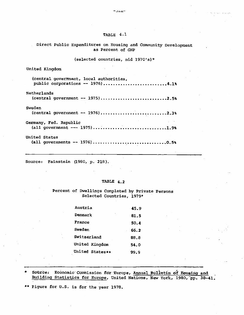
TABLE 4.1

Direct Public Expenditures on Housing and Community Developmentas Percent of GNP

(selected countries, mid l9701s)*

United Kingdom

(central government, local authorities,public corporations —- 1976) 4.1%

Netherlands(central government —— 1975) 2.5%

Sweden(central government —- 1976) 2.3%

Germany, Fed. Republic(all government ——. 1975) 1.9%

United States(all governments —— 1976) 0.5%

Source: Fainstein (1980, p. 218).

TABLE 4.2

Percent of Dwellings Completed by Private PersonsSelected Countries, 1979*

Austria 45.9

Denmark 81.5

France 50.4

Sweden 66.2

Switzerland 88.8

United Kingdom 54.0

United States** 99.9

* Source: Economic Commission for Europe, Annual Bu1ltin of Housiz andBuilding Statistics for Europe, United Nations, New York, l98O,.pp. 38—41.

** Figure for U.S. is for the year 1978.

—53—

economic literature has focused on three allegations: Public housing is

produced inefficiently; it is an inefficient method for distributing income

to the poor; and it has anomalous distributional implications. Each of these

is discussed in turn.

4.1 Production Inefficiency

As noted above, for a considerable portion of its history, the federal

government paid for the capital costs of public housing, but did not subsidize

operating costs. To assess the efficiency implications of this practice,

Muth (1973) assumes that housing services are produced with two inputs, "real

estate inputs," which are used to build a structure, and "current inputs,"

which are used to maintain it. Presumably, there is some scope for sub-

stitution between them. For example, one can use relatively expensive

aluniinwn siding which requires little maintenance, or wood siding, which

is cheaper but needs more maintenance. The necessary condition

for cost minimization is that the marginal rate of substitution between

the inputs be equal to theratio of their marginal social costs.

Because capital Costs are paid ky the federal government, local authorities

in effect face a price of capital below its social marginal cost. This

gives them an incentive to produce housing which uses too much capital and

too little maintenance.

—54—

Nuth's formal analysis focuses on the costs of this distortion in

input ratios.46 He postulates a constant elasticity of substitution unit

cost function for housing services:

(4.1) h = (1—) +

where = price per unit of housing services, r = price per unit of real

estate inputs, c = price per unit of current inputs, = elasticity of

substitution between real estate inputs and current inputs, and , is a

parameter of the production function.

On the basis of earlier studies on production in housing, Muth assumes

that = 0.2 and 4.i = .243. He normalizes prices such that in the private

sector r = 1 and c = 1. To the extent the public housing authority pays for

its operating expenses, it also faces a price of c equal to one. On the

other hand, due to the federal subsidy, the authority's effective value of

r is only about .05.

Substituting these figures into equations for input ratios derived from

(4.1), l4uth shows how the subsidy lowers the per unit price of housing

produced by the housing authority, and induces it to use relatively less

in the way of current inputs than the private sector. But the key question

is what the resource cost of public housing is. This is found by pricing

the inputs used by the local housing authorities at their market prices.

Muth finds that the ratio of the market value of public housing to its

resource cost is 0.82. Other studies using, methodologies somewhat

46 Muth (1973, p. 7) notes two other reasons why public housing tends to bemore expensive than comparable private housing: (1) The Davis—Bacon Act forcescontractors to use wage scales set by the Department of Labor. These tend to behigher than those prevailing in the labor market. (2) Cleared slum land isoften used, and such land tends to be expensive due to proximity to downtownareas. Demolishing existing structures is also expensive.

-.55—

different than Muth's have found estimates of production inefficiencies

similar in magnitude.47 (See Weicher (1979, p. 497)).

In 1970, it was decided to reimburselocal housing authorities for the

excess of operating costs over revenues. As Olsen (forthcoming,p.9) notes,

in effect this reduces theprice of marginal maintenance and rehabilitation

facing the authorities to zero.Operating costs increased dramatically,

and by 1976 federal operating subsidies mounted to 40 percent of the operating

costs of public housing units. However, in many programs today, there are

still mortgage subsidies which gerteratea bias toward capital intensive

production techniques. There is also a persistent belief that publicly

constructed housing is excessively expensive because public sector managers,unlike their counterparts in the private sector, have no incentive to give

much weight to efficiency.Unfortunately, no systematic estimates of the

importance of this effect are available.Similarly, despite the widespread

publicity given to occurrences of outright corruption in the administration48

of public housing , it is not clear what the impact of this has been on its

cost.

4.2 Consumption Inefficiency

An important motivation behind public housing appears to be income

redistribution. Given the theoretical presumption that redistributing

income via a price subsidy is inefficient relative to cash, the key

empirical question is whether the inefficiency is large in dollar terms.

47 Of course, the validity of such estimates must be viewed in lightof the methodological difficulties in studying housing supply discussedin Section 2.

48. In 1982, one member of the Chicago Housing Authority (CHA) opinedthat "The CHA is a political slop bucket, and everybody's drinking fromit." (Newsweek Magazine, April 19, 1982.)

—56-

An early examination of this issue is due to Aaron and Von Furstenberq

(1971). They assume that a representative individual's utility (U)

depends only upon his consumption of housing services, h (which are

defined so that the price of a unit equals one dollar) and all other goods

G:

U = U(Q,G)

Facing private market prices, the individual chooses some bundle

(Q,G°) , with associated utility level U0 . Now suppose the government

makes available to the individual the opportunity to purchase housing

services at a price of (l-s) , where s is the subsidy rate. Geometric-

ally this is equivalent to pivoting out the budget line. In general, the

individual will change his consumption bundle to (Q,G1) , which -

gives utility U1 > U0 •49 The cost to the government of the program is

:1.

The problem is to find the amount of income that would be reqtaired

for the recipient to attain, at market prices, the level of utility Ut

reached under the subsidy program. This is found simply by holding the

price of housing at its original value, and giving the individual lump

sum income until his utility reaches U . (The geometrical analogue is

a parallel shift outward of the budget line until it is just tangent to

the indifference curve associated with UCall the amount of lump sum

49 If the individual is not allowed to choose freely the quantity

of subsidized housing he consumes, his utility may be less than U1.

In the extreme case where the housing authority offers a specific

quantity-price bundle, the budget line does not pivot. The program

simply adds one point to the family's budget set.

—57—

income so required N . Then Aaron and Furstenberg define the relative

consumption inefficiency of the subsidy as

sQ-N

sQh

To implement this theoretical framework, one needs to choose a

utility function and specific values for its parameters. Aaron and von

Furstenberg assume a constant elasticity of substitution utility function.

Parameters are selected so that they are consistent with a price elasti-

city of demand for housing of -l.0 and an income elasticity of 1.0.

Assuming that the public housing subsidy rate is 50% (i.e., s—OS),

they find that the relative consumption inefficiency is about 10%.

The price and income elasticities used by Aaron and von Furstenberg

to compute the utility function parameters are from studies of the housing

behavior of the general population. It might very well be the case, how—

ever, that the behavioral responses of the poor differ from those of the

population at large. Moreover focusing on a representative individual

does not allow one to address the important question of how benefits vary

across individuals. Subsequent to the Aaron-von Furstenberg study, a number

of others have been done which estimate utility function parameters with• -

cross sectional data on public housing recipients. This allows a more ac-

curate depiction of the behavioral and distributional effects of the subsidy.

We discuss here the analysis by Murray (1980), which is one of the most

recent and careful.

50 See also Kraft and Kraft (1979), Kraft and Olsen (1977) , Suzuka and,

Stegman (1978) , and Olsen and Barton (1982)

—58-

Murray assumes that preferences can be represented by the genera1izei

constant elasticity of substitution form

C2(4.2) U lh + G )

where the C's are parameters to be estimated, and the other variables

are as defined above.51 The first order conditions for utility maximization

imply that

____ C1C(4.3)

gh=

.c3+ -) £n + (2-c3) 2,n G

Murray partitions his sample into groups based on family size, and for

each group estimates (4.3) using aninstrumejital variables technique.

The' variable p is based upon the Bureau of Labor Statistics (BLS)

estimate of the price of a "standard" unit in each city. The quantity of

housing services provided by a given dwelling i Ito rent divided by the

rental on the BLS standard unit. (Inter-city price indices are formed by'

taking the ratio of the prices of the BLS units in the different cities.)

Because market rents are unavailable for public housing units, it

is not clear how to measure the quantity of housing services they provide.

(Recall the discussion of Section 2.concerning the difficirlties of measuring

.housing services. in general.) To estimate the market value of each pubUc

houág unit, Murray uses an hedonic price equation produced by another study

By substituting into the hedonic equation the characteristics of a given

51. The version of this equation appearing in Murray's paper has a typo-graphical error (equation 1, p. 27).

—59—

public housing dwelling, he can obtain an estimate of what its rent would

be in the private market.52

Equation (4.3) is estimated with 19.71 data on nearly 1400 successful

public housing applicants across evèn cities. The parametersp1y. tha

dn aVerage, the.subsidy increased housl.ng consumption by about 95% oér what it

would have been otherwise. (p.33). If.aoh household would have received

instead axv equivalent cash grant, housing consumption would have increased

only 0% above the unsubsidized level.

To assess the efficiency of the program, Murray computes the subsidy

cost associated with each public housing unit, defined as the resource cost

of the unit53 plus administrative costs minus the rent paid. He finds that

in his sample, the average subsidy cost is $1530, while the average nominal

benefit is $94954 Thus, a shift to an equivalent cash grant would lower

costs by 34%. Other studies have reached similar conclusions. (See Weicher

(1979, p. 497)).

Although the results of such analyses have contributed considerably

to our understanding of public housing, they suffer from several potentially

important problems. The fact that the utility function parameters are esti-

mated using only public housing inhabitants means that the estimates may be

inconsistent due to selectivity bias.55 The use of hedonic indices to value

public housing units is also problematic because, as Aaron (1977, p. 69) has

noted, public housing tenants may not value housing characteristics the sarna

way that the market would.

52 The hedonic price equation is based on data from New York City.

53 Building on research similar to that described in Section 4.1, Murrayassumes that the resource cost exceeds the market value of the unit by 17percent.

54 There is considerable variation in these figures across families.

5 For a discussion of this statistical problem, see Heckman (1979)

—60—

Even if the parameter estimates were perfect, errors in measuring con—

suxnption inefficiency might arise due to the implicit assumption that the

only distortion in the system is the subsidy on housing. For example, it is

well-known that the welfare system tends to place high implicit marginal tax

rates on the labor income of the poor. Analyses of public housing subsidies

shou'd therefore also take work decisions into account. However, it is dif-

ficult to say a priori in what direction current estimates are biased by the

failure to do so.

4.3 Distributional Implications

The studies by Murray and others have shown that public housing

confers a relatively large benefit upon the recipients. However, this

benefit is available only to a small number of poor people. As noted

above, there are a few million public housing units, but in 1979, there

were about 25 million persons whose income fell below the U.S. govern—

56ment poverty line. Hence, many more people desire entry into publ.ic

housing than it is possible to acconodate. It turns out that although -

the incomes of the recipients are concentrated at the bottom of the in-

come distribution, many people gain entry who arebetter off than those

who do not. (See Aaron (1972, p. 115)1

A related issue is the distribution of benefits within the group

of families who actually gain admittance. Murray (1980, p. 31) regressed

his estimates of the actual benefit on annual income, holding constant

various demographic characteristics of the families. He found that there

is indeed a negative relation between income and benefits. But the R2 of

56 Statistical Abstract of the United States, (1980, p. 465.)

—61—

the equation is only O.7O, suggesting that there is quite a bit of ranciomness

in the way the benefits are distributed across tenants.

Aaron (1972, p. 12) has pointed out that public housing may have gen-

eral equilibrium effects with important distributional implications. Pre—

sumably, the availability of public housing decreases the demand for low-cost

non—subsidized housing, lowering the rents in that sector. This would tend

to increase the real incomes of the tenants and lower the real incomes of

the landlords. These issues do not yet appear to have received econometric

attention.

4.4 Possibilities for Reform

The consensus from the literature is that public housing is ineffi-

ciently produced, distorts consumption patterns on the part of the bene-

ficiaries, and redistributes income capriciously.57 Most economists have

been against the program for years. Muth's (1973) sentiment is probably

typical: "The only possible justification for housing programs I can see

is that they are politically feasible whereas increased income maintenance

is not.". (p. 43)

It has been suggested that if subsidies have to be maintained, then

their link to public provision of housing should be broken. If the subsidy

could be applied to private sector housing, then it would no longer be nec—

57 We have not touched upon the administrative coxnple:ity of theprogram and the associated costs. Mills (undated) p. 26 notes, "...a cadre of specialized talent has sprung up to advise building landlordsand tenants on procedures to find their way through r around thebureaucratic maze...".

—62—

essary for the public sector to get involved in apartment construction and

management. In addition, recipients of aid would rio longer be geographic-

ally concentrated and marked publicly.

As noted above, under the Section 8 program, there are indeed subsidies

for low income individua who rent on the private market. However, as of

19Th, only about 1.3% of publicly subsidized dwellings for the poor were

associated with demand side programs (Quigley (1980, p. 162)). And even under

Section 8, recipients are limited in their choice of dwellings, cannot

spend more than 25% of their incomon rent, and can only choose front land-

lords who participate in the program.-

demand oriented subsidy program that has received a good deal ofattention is "housing allowances.'58Each qualified individual would receive

from the government a payment equal to the difference between the cost ofstandard housing established by the program and some fraction of his income.

The allowance could be spent on any housing on the private market, providing

that it met certain quality standards. Recently, a large social experiment

(the Experimental Housing Allowance Program) was conducted in several citiesto determine how housing allowances would affect people's behavior.5 Analyses

of the data by Hanushek and Quigley (1981, p. 204) and Venti and Wise (1982)

suggest a moderate effect upon housing consumption; the income elasticity of

demand for housing services in the experiment was below 0.5. Interestingly,the increased demand generated by the housing allowances does not seem to

58 A number of alternative policy approaches are discussed in CongressionalBudqet OUice (1982).

59 For details on the design of the experiment and its results, seeBradb.iry and Downs (1981).

—63-

have had much effect upon housing prices in the communities where the expe—

irnent was conducted. This is probably because the supply of housing services

is fairly elastic and the response to the increased allowance takes place

gradually over time.

The main problem with the housing allowances system examined in the

experiment is the stipulation that the dwellings meet various quality

standards. The purpose of this provision is presumably to protect the poor

from unscrupulous landlords who would take their money and provide no

services in return. The evidence from the experiment indicates that it

would be very hard to set sensible standards and that enforcement would entail

substantial administrative costs. In addition, the imposition of standards

reduced participation in the program significantly (Allen et al. (1981, 26)) -

Nuth (1973) has proposed the introduction of "rent certificates,"

which could be used by the poor to pay for their rents in any public or

private housing that they deemed reasonable. Such a program comes very

close to being an unrestricted cash transfer. Clearly, there are power—•

ful interest groups which, for one reason or another, wish to see income

support for the poor closely linked to their consumption of housing.

Whether or not a scheme like Muth's is perceived to be tied closely enough

to housing to be politically acceptable is an open question.

5. Conclusions

Empirical investigation of the effects of government policies upon

housing behavior presents researchers with difficult methodological

problems. Given that there is no "best" way for dealing with these

problems, investigators are bound to produce different answers. Never—

—64—

theless, there appears to be widespread agreement that in the United

States, the income tax treatment of owner-occupied housing and the pui1jc

provision of low—income housing have substantially increased the consumption

of housing services. In the process, economic efficiency has decreased.

Moreover, the housing related provisions in the federal income tax

have lead to a more unequal distribution of income. It is unlikely that the

disequalizing effects of these provisions have been mitigated by the equalizing

effects of the expenditure programs. Thus, judged by the standards of con—

ventiona]. welfare economics, reform seems appropriate, and we have discussed

a number of possibilities. Of course, it might be that current programs are

moving us toward important social and political goals that lie outside the

scope of welfare economics. But given that these goals have never been care-

fully articulated, it is impossible to tell whether or not such is the case..

—65-

Aaron, Henry, 1972, Shelters and Subsidies, (Washington, D.C.: The Brookings

Institution.

Aaron, Henry J. and George N. von Furstenberg, June 1971, The Inefficiency

of Transfers in Kind: The Case of Housing Assistance, Western Economic

Journal, pp. 184-191.

Aaron, Henry, 1977, Comments, in Juster F. Thomas (ed.), The Distribution of

Economic Well-Being, (Ballinger Publishing Company), pp. 65-69.

Abbott, Michael, and Orley Ashenfelter, October 1976, Labor Supply, Commodity

Demand, and the Allocation of Time, Review of Economic Studies 43,

pp. 389—411.

Alexander, W. E., Comment, Annals of Economic and Social Measurement 4,

pp. 175—178.

Allen, Garland E., Jerry J. Fitts, and Evelyn S. Glatt, 1981, The Experiuenta1

Housing Allowance Program, in Bradbury, Katharine J. and Anthony Downs

(eds.), Do Housing Allowances Work?, (Washington, D.C.: The Brookings

Institution), pp. 1—32.

Atkinson, A. B., 1970, On the Measurement of Inequality, Journal of Economic

Theory 2, pp. 244—263.

Atkinson, A. B., 1977, Housing Allowances, Income Maintenance and Income

Taxation, in Feldstein, N. S. and R. P. Inman (eds.), The Economics of

Public Services, (Macmillan, London).

—66—

Bradbury, Katharine L. and Anthony Downs, 1981, (eds.), Do Housing Allowances

Work?, (Washington, D.C.: The Brookings Institution).

Brown, James N. and Harvey S. Rosen, Nay, 1982, A Note on the Estimation of

Structural Hedonic Price Nodels, Econometrica 50, pp. 765-768.

Carliner, Geoffrey, 1973, Income Elasticity of Housing Demand, Review of Economics

and Statistics 55, pp. 528—532.

Congressional Budget Office, September 1981, The Tax Treatment of Homeowner—

ship: Issues and Options, (Congress of the United States).

Congressional Budget Office, May 1982, Federal Housing Assistance: Alternative

Approaches, (Congress of the United States).

de Leeuw, Frank and Raymond J. Struyk, 1975, The Web of Urban Housing,

(Washington D.C.: the Urban Institute).

Diamond, Douglas B. and Barton A. Smith, 1981, Housing as an Explicit 'Good,'

(North Carolina State University, mimeo).

Englund, Peter and Mats Persson, forthcoming, Housing Prices and Tenure

Choice With Asymmetric Taxes and Progressivity, Stockholm School of

Economics, Journal of Public Economics.

Fainstain, Susan S., 1980, American Policy for Housing and Community Develop-

ment: A Comparative Examination, in Montgomery Roger and Dale Marshall

(eds.) Housing Policy in the 1980's, (Lexington Books, D.C. Heath and

Company), pp. 215-230.

-67-

Feldstein, Martin S., July-August 1976, On the Theory of Tax Reform,

Journal of Public Economics 6, pp. 77-104.

Feldstein, Martin S., September 1981, Inflation, Tax Rules, and the Accumu-

lation of Residential and Nonresidential Capital,National Bureau of

Economic Research, Working Paper No. 753.

Pollain, James R., Jr., May 1979, The Price of Elasticity of the Long-Rw

Supply of New Housing COnstruction, Land Economics 55, pp. 190—199.

Hanushek, Eric A. and John M. Quigley, 1981, Consumption Aspects, in

Bradbury, Katharine L. and Anthony Downs (eds.), Do Housing Allowances

Work?, (Washington D.C., Brookings Institution), pp. 185—240.

Beckman, James, January 1979, Sample Bias as a Specification rror,Econometrica 47:1, pp. 153—162.

Hendershott, Patric H. and Sheng Cheng Hu, July 1981, The Allocation ofCapital Between Residential and Nonresidential Uses: Taxes, Inflation

and Capital Market Constraints, National Bureau of Economic Research

Working Paper No. 718.

Hendershott, Patric H. and James D. Shilling, September 1980, The Economics

of Tenure Choice, 1955-79, National Bureau of Economic Research,

Working Paper No. 543.

Hendershott, Patric B. and Joel Slemrod, 1981, Taxes and the User Cost of

Capital for Owner-Occupied Housing, The Ohio State University, inbneo.

Henderson, J. V. and Y. loannides, September 1981, A Model of Housing Tenure

Choice, Brown University, Working Paper No. 81-27.

—68—

Hughes, G. A., Housing and the Tax System, 1980, in Hughes, G. A. and

C. N. Heal, (eds.), Public Policy and the Tax System, (Boston: George

Allen and Unwin), pp. 67—105.

Ingrain, Gregory K. and Yitzhak Oron, 1977, The Production of Housing Services

from Existing Dwelling Units, In Ingram, Gregory K. (ed.) Residential

Location and Urban Housing Markets, (Cambridge, NA.: Ballinger

Publishing Company), pp. 273-314.

Jaf fee, Dwight 14. and Kenneth T. Rosen, 1979, Mortgage Credit Availability

and Residential Construction, Brookings Papers in Economic Activity 2,

pp. 333—76.

Jones, Reginald H., December 1978, Sunset Legislation, Tax Review.

Jorgenson, Dale W., December 1971, Econometric Studies of Investment Behavior:

A Survey, The Journal of Economic Literature, pp. .1111-11.47.

Kearl, J. R., October 1979, Inflation, Mortgages, and Housing, Journal, of

Political Economy 5, pp.. 1115—1138.

King, Mervyn A., October 1980, An Econometric Model of Tenure Choice and

Demand for Housing as a Joint Decision, Journal of Public Economics,

pp. 137—160.

King, Mervyn A., March 1981, The Distribution of Gains and Losses from

Changes in the Tax Treatment of Housing, London: Social Science

Research. Council Programme, No. 20.

King, Mervyn A., forthcoming, An Index of Inequality: with ApplicatiOnS to

Horizontal Equity and Social Mobility, Econometrica.

—69—

Kraft, John and Arthur Kraft, 1979, Benefits and Costs of Low Rent Public

Housing, Journal of Regional Science 19, No. 3, pp. 309—317..

Kraft, John and Edgar 0. Olsen, 1977, The Distribution of Benefits from

Public Housing, in Juster, F. Thomas ted.), The Distribution of Economic

Well—Being, (Ballinger Publishing Company), pp. 51—65.

Laidler, David, 1969, Income Tax Incentives for Owner—Occupied Housing, in

Harberger, Arnold C. and Martin J. Baily, (eds.) The Taxation of Income

from Capital, (Washington, D.C.: The Brookings Institution).

MacRae, C. Duncan and Nargery Austin Turner, 1981, Estimating Demand for

Owner-Occupied Housing Subject to the Income Tax, Journal of Urban

Economics, 10, pp. 338—356.

Mayo, Stephen K., July 1981, Theory and Estimation in the Economics of

Housing Demand, Journal of Urban Economics 10, Pp. 95—116.

Mills, Edwin S., undated, National Housing Policy: A Critique and a Proposal,

Princeton University, mimeo.

Murray, Michael P., 1980, Tenant Benefits in Alternative Federal Housing

Programs, Urban Studies 17, pp. 25—34.

Murray, Michael P., undated, Subsidized and Unsubsidized Housing Stocks:

1961—1977, Claremont Graduate School, mimeo.

Nusgrave, Richard A., 1959, The Theory of Public Finance, New York: McGraw—

Hill.

—70--

Muth, Richard F., 1973, Public Housing — An Economic Evaluation, (Washington,

D.C.: American Enterprise Institute).

Nuth., Richard F., March 1982, Effects of the U.S. Tax System on Housing

Prices and Consumption, Hoover Institution, Working Paper No. E—82-3.

Nichols, Albert L. and Richard J. Zeckhauser, May 1982, Targeting Transfers

Through Restrictions on Recipients, American Economic Review Papers and

Proceedings 72, pp. 372—377.

Niskanen, W. A., Jr., 1971, Bureaucracy and Representative Government,

Chicago: Aldine.

Olsen, Edgar 0., forthcoming, Implications of the Experimental Housing

Allowance Program for Housing Policy, in Joseph Friedman and Daniel

Weinberg (eds.), The Great Housing Experiment.

Olsen, Edgar 0. and David M. Barton, February 1982, The Benefits and Costs

of Public Housing in New York City, The Jefferson Center for Political

Economy, Discussion Paper No. 123.

Polinsky, A. Mitchell and David T. Eliwood, May 1979, An Empirical Reconcili-

ation of Micro and Grouped Estimates of the Demand for Housing, Review

of Economics and Statistics LXI, pp. 199—205.

Poterba, James N., 1980, Inflation, Income Taxes and Owner—Occupied Housing,

National Bureau of Economic Research, Working Paper No. 553.

—71--

Quigley, John .M., 1980, Housing Allowances and Demand-OrientedHousing

Subsidies, in Montgomery, Roger and Dale Marshall (eds.) Housing Policy

in the 1980t5, Lexington Books, D. C. Heath and Company, 161-68.

Quigley, John M., September 1982, Non—Linear Project Constraints and Consumer

Demand: An Application to Public Programs to Residential Rousing,

Journal of Urban Economics.

Rosen, Harvey S.., February 1979, Rousing Decisions and the U. S. Income Tax:

An Econometric Analysis, Journal of Public Economics 1]., pp. 1—23.

Rosen, Harvey S., 1981, Comments, in Aaron, H. 7. and J. A. Pechinan (eds.),

How Taxes Affect Economic Behavior, (Washington, D. C.: The Brookings

Institution), pp. 323—326.

Rosen, Harvey S. and Kenneth T. Rosen, February 1980, Federal Taxes and

Homeownership Evidence from Time Series, Journal of Political

Economy 88, pp. 59-75.

Rosen, Sherwin, 1974, Hedonic Prices and Implicit Markets: Product Differ-

entiation in Pure Competition, Journal of Political Economy 82, pp. 34—55..

Rothenberg, Jerome, 1977, Comments on Chapter 8, in Ingram, Gregory K., (ed.)

Residential Location and Urban Housing Markets, (Cambridge, MA: Eallinger

Publishing Company), pp. 315—321.

Rydell, C. Peter, September 1979, Shortrun Response of Housing Markets toDemand

Shifts, Rand Corporation, Working Paper R-2453-HUD.

—72—

Sandmo, Agnar, July 1976, Optimal Taxation—- An Introduction to the Literature,

Journal of Public Economics,6, No. 12, pp. 37-54.

Straszheim, Nahion R., 1980, The Section 8 Rental—AssiStance Program: Costs

and Policy Options, in Montgomery, Roger and Dale Marshall (eds.), Housing

Policy for the 1980's, (Lexington Books), pp. 169—184.

Struyk, Raymond J., 1976, Urban HomeownerShiP, (Lexington, MA: Lexington Books).

Struyk, Raymond J., 1978, Sue A. Marshall and Larry J. Ozanne, Housing Policies

for the Urban Poor, (Washington, D.C.: The Urban Institute).

Suxnka, Howard 3. and Michael A. Steginan, 1978, An Economic Analysis of Public

Housing in Small Cities, Journal of Regional Science 18, No. 3, pp. 395—410.

Summers, Lawrence, December 1980, Inflation, the Stock Market and Owner-Occupied.

Housing, National Bureau of Economic Research, Working Paper No. 606.

Sunley, Emil N., 1981, Comments,in Aaron, Henry 3. and J. A. Pechinan, How

Taxes Affect Economic Behavior, (Washington, D.C.: The BrookingS Institution),

pp. 127—130.

Tobin, James, 1970, On Limiting ths Domain of Inequality, Journal of Law and

ECOnOmiCS 13, pp. 263—277.

Venti, Steven F. and David A. Wise, 1982, Moving and Housing Expenditure:

Transactions Cost and Disequilibrium, Harvard University, mimeo.

—73—

Weicher, John C., 1979, Urban Housing Policy, in Mieszkowski Peter and -

Nahion Straszheim, Current Issues in Urban Economics, The Johns Hopkins

Press, pp. 391.

Weicher, John C., 1980, Housing —- Federal Policies and Programs, (Washington,

D.C.: American Enterprise Institute).

Weiss, Yoraxn, 1978, Capital Gains, Discriminatory Taxes, and the Choice Between

Renting and Owning a House, Journal of Public Economics 10, pp. 45—55.

White, Michelle 7. and Lawrence White, The Subsidy toOwner-Occupied Housing:

Who Benefits? Journal of Public Economics 7, pp. 111—126.